1

WiFinder, a Wifi Signal Intensity Mapping RobotChaitanya Aluru, Sean Roberts, and Eric Wu

I. INTRODUCTION

The goal of the WiFinder project is to develop a robot thatwill find the strongest 802.11 signal in a room. In order todo this, the robot first maps out the 802.11 signal intensityusing RSSI measurements, and then find the position ofmaximal signal strength intensity within the mapped area. Indoing so, the robot implicitly solve the localization problemover a large, two dimensional grid. This requires the carefulintegration of several sensors, and precise control over therobot’s movements. Here, we describe the implementation ofour robot, model the behavior of the sensors used to localizeand control the robot, and simulate the errors that arise due toimperfect sensor readings and errors in control.

The GitHub repository for this project is https://github.com/wueric/WifiRobot, and the demonstration video for the projectis located at http://youtu.be/C c6Be1Nw74.

II. MAXIMAL SIGNAL STRENGTH ALGORITHMS

We manually constructed several spatial maps of RSSI,which are shown below. We conducted measurements in mul-tiple passes, to determine the amount of variability in signalintensity. While the general shapes of the spatial signal profilewere approximately the same for the two passes, there werealso major differences. These differences in the shape of theprofile suggest that 802.11 signal strength is quite variable andunpredictable, making hill-climbing and other such algorithmsinfeasible and unlikely to result in finding a point of maximalstrength.

As a result, we implemented simple, search-and-maximizealgorithm. Rather than dynamically determine where to search,the algorithm prescribes a fixed rectangular grid pattern for therobot to trace out. The robot measures RSSI signal intensityat fixed distances along this grid, and then returns to the pointof maximal signal intensity at the end of its search.

These algorithms were implemented using a state machinearchitecture, similar to the ones implemented in the courselabs.

III. HARDWARE AND FIRMWARE

Our wifi-seeking robot was based upon the iRobot Createplatform, manufactured by iRobot corporation. Our primarycomputational platform for the project was the FreescaleKL25Z ARM microcontroller running the mbed framework.The iRobot Create was interfaced to the mbed board usinga serial port. Because the iRobot Create required 5 V inputsignals, we were required to use a Sparkfun logic levelconverter to interface the iRobot with the mbed electrically.The serial connection between the iRobot and the mbed boardwas implemented using the Serial framework developed by thembed team. Instructions were sent to robot using the iRobot

Fig. 1. Photograph of the iRobot Create electronics bay. The MaxbotixLV-EZ1 is on the forward-facing breadboard and is used to sense distancetravelled. Inside the electronics bay we have a Honeywell HMC5883L mag-netometer, an Adafruit CC3000 WiFi breakout board, a SparkFun BlueSMiRFBluetooth modem, and a SparkFun logic level converter. All of these devicesare integrated with a Freescale KL25Z microcontroller running the mbedplatform.

Create Open Interface with code developed by our projectgroup.

We used the Adafruit CC3000 WiFi shield as our 802.11signal intensity sensor. The wifi shield was interfaced to thembed using the SPI interface and the mbed cc3000 librarydeveloped initially by cc3000 chip manufacturer Texas Instru-ments and ported to the mbed platform by Martin Kojtal. Inaddition, we used a SparkFun BlueSMiRF Bluetooth modemto interface the robot with a Bluetooth-enabled laptop in orderto send robot position coordinates and signal intensity readingsto the laptop. This modem was interfaced to the KL25Z boardusing a serial port, using the Serial framework.

To help determine the robot’s position, we used an ul-trasound sensor to measure distance and a magnetometer tomeasure angular orientation. The ultrasound sensor was aMaxbotix LV-EZ1, put on a breakout board by Adafruit. Thissensor was interfaced to the KL25Z using an analog connection(to conserve the KL25Z’s limited number of serial ports).Data was read off of the LV-EZ1 using the KL25Z’s onboardanalog-to-digital converter (ADC) using the mbed AnalogInlibrary. Our magnetometer was a Honeywell HMC5883L 3-axis digital compass, put on a breakout board by SparkFun.The magnetometer was electrically interfaced to the KL25Zusing an I2C connection, and was interfaced through softwareusing code originally authored by Tyler Weaver, and modifiedby the project group to support sensor calibration.

A photograph of our hardware is provided in Figure 1, anda block diagram illustrating our hardware setup is provided inFigure 2.

2

mbed% Logic%%converter%

cc3000%

iRobot%

BlueSMIRF%

MaxBo;x%%LV=EZ1%

HMC5883L%

Fig. 2. Block diagram for our hardware setup.

IV. CHARACTERIZING AND MODELING SENSORS

e had a variety of sensors to choose from to aid us inlocalization. Our requirements were to be able to solve thelocalization problem on a grid up to 10 meters per side towithin +/- 1

3 m. To do this, we needed to be able to moveforward one unit of distance at a time, and turn as closeto 90 degrees as possible at the edges of the grid. For theforward motion, we considered the onboard accelerometer, anultrasound module.

A. AccelerometerTo determine the accuracy of the accelerometer module,

we laid it flat at rest on a table and read the measuredacceleration values at one second intervals. In addition to this,we added integration code to measure the distance traveled bythe robot in each direction. Initially, it measured about 2-3 m

s2

on each axis. We realized that most of the error was systematicerror, which could be removed. As a basic first step, we tookthe average of the first ten readings from the accelerometer,and subtracted this value from subsequent readings. Afteradjusting for bias, the readings were surprisingly accurate,usually within 0.1 m

s2 on each axis. Unfortunately, even thissmall error quickly compounded. Within five readings, theintegrated position was already about 0.3 m off on each axis,or about a foot in each direction. This level of inaccuracywas unacceptable for us. Although there are more advancedfiltering techniques which could have gotten us better results,we realized that the accelerometer was unlikely to work for us.This is because the iRobot moves at a relatively slow velocity,and all of the acceleration is done in very short bursts. Inorder for an accelerometer to work in such conditions, thesampling rate must be very high during acceleration. Combinedwith heavy filtering code, the accelerometer would consume asignificant portion of the processor’s clock cycles, which couldpotentially conflict with other sensor readings and controllingthe robot. Furthermore, since using dead reckoning requiresthat the accelerometer be continuously sampled, using it wouldintroduce substantial concurrency issues in our software. For

60 80 100 120 140 160 180 200 220 240 2602000

3000

4000

5000

6000

7000

8000

9000

10000

11000

12000

True distance (cm)

16 b

it se

nsor

read

ing

Student Version of MATLAB

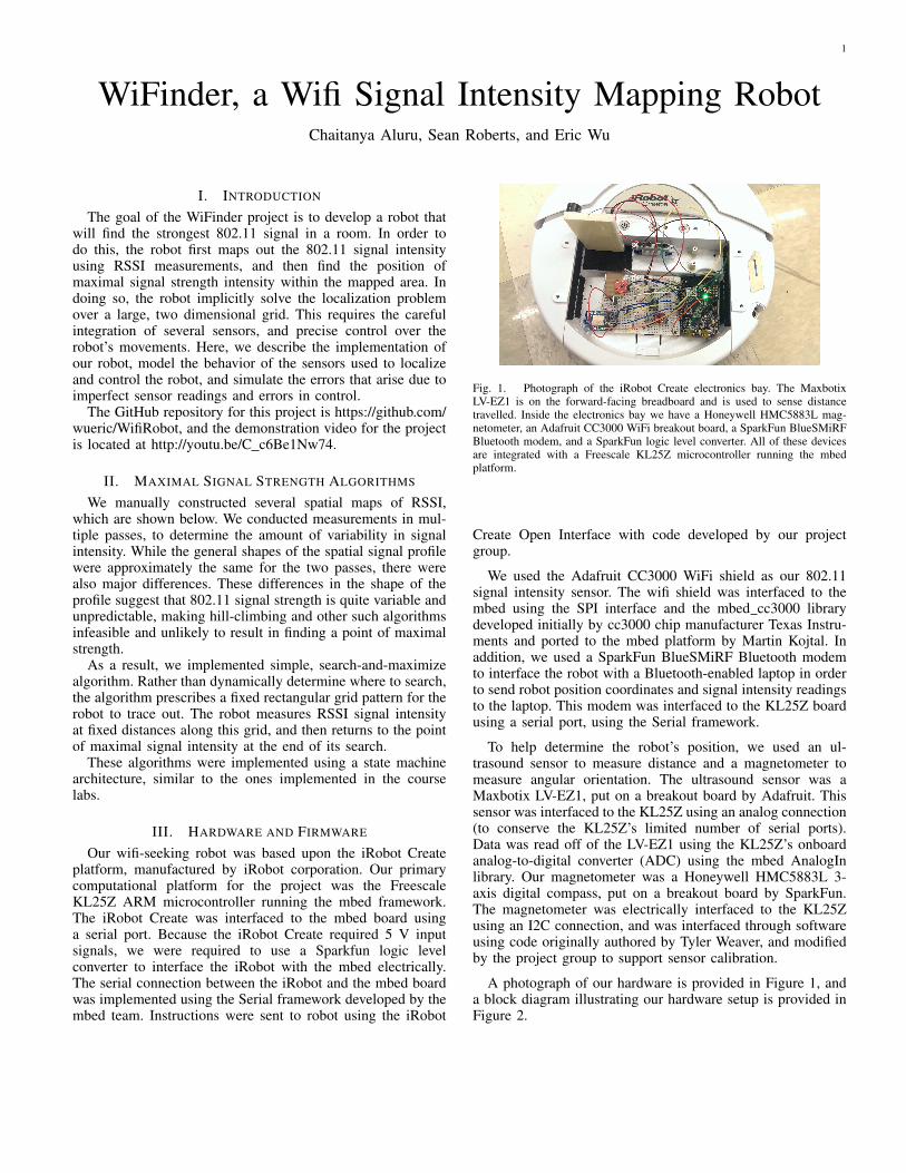
Fig. 3. Plot showing 16-bit ADC values for the LV-EZ1 ultrasoundrangefinder plotted against the true distance of an object placed in front ofit. The plot is very linear, which suggests that the sensor response can bemodeled with the affine model.

these reasons, we decided to perform localization using othersensors.

B. Ultrasound RangefinderIn order to accurately measure distance travelled using the

Maxbotix LV-EZ1 ultrasound sensor, we first had to model andcalibrate the sensor. This was done by connecting the analogoutput of the LV-EZ1 (where VCC for the sensor was set to therecommended 3.3 V) to the KL25Z’s onboard 16-bit analog-to-digital converter (ADC). We took data points by placing alarge flat surface at 60 cm increments in front of the sensorand reading off the value returned by the ADC. The results ofthese measurements are plotted in Figure 3.

Because the sensor response was approximately linear withdistance, we modeled the response of the analog output ofthe LV-EZ1 coupled ADC using the affine model of a sensor.Briefly, the output of the sensor is modeled as

f(x(t)) = a · x+ b

where f is the output of the sensor, and x is the truedistance. Using MATLAB, we were able to calculate best-fitvalues for parameters a and b. According to these calculations,a was 50.18 bits

cm and b was -292 cm. The affine model wasthen implemented in software using these values to accuratelydetermine distance travelled.

C. MagnetometerIn order meaningfully read orientation from the HMC5883L

magnetometer, the magnetometer had to be calibrated to offsethard-iron effects and soft-iron effects. Hard-iron effects corre-spond to magnetic fields that generate a generate a consistent,constant offset to the magnetometer readings. They correspondto permanent sources of magnetic fields (in our case, the mag-nets and coils for the iRobot’s motors contributed significantly

3

200 300 400 500 600 700 800

−600

−550

−500

−450

−400

−350

−300

−250

−200

−150

−100

Best fit: R = 280.6; Ctr = (498.0,−366.0)

Student Version of MATLAB

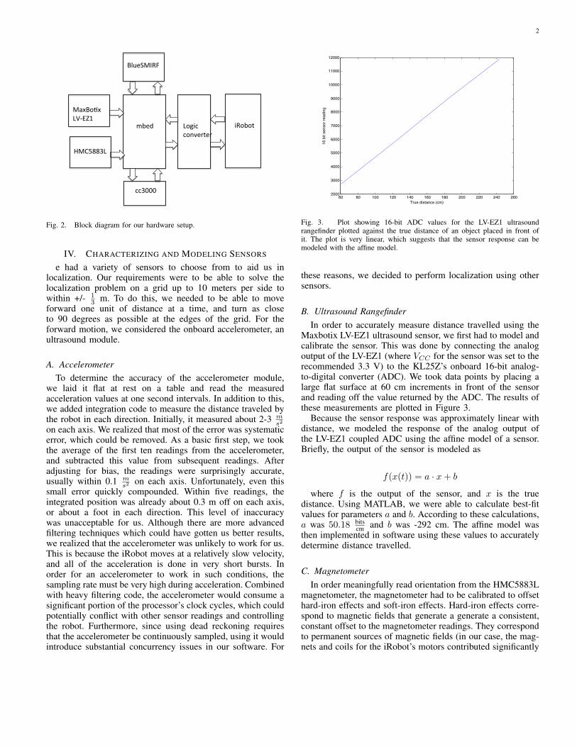
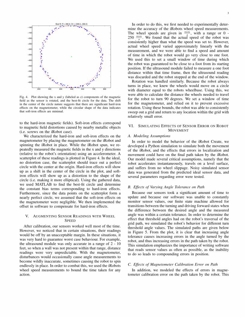
Fig. 4. Plot showing the x and y (labeled as z) components of the magneticfield as the sensor is rotated, and the best-fit circle for the data. The shiftin the center of the circle nature suggests that there are significant hard-ironeffects on the magnetometer, while the circular shape of the data indicatesthat soft-iron effects are minimal.

to the hard-iron magnetic fields). Soft-iron effects correspondto magnetic field distortions caused by nearby metallic objects(i.e. screws on the iRobot case).

We characterized the hard-iron and soft-iron effects on themagnetometer by placing the magnetometer on the iRobot andspinning the iRobot in place. While the iRobot spun, we re-peatedly measured the magnetic fields in the x and y directions(relative to the robot’s orientation) using an accelerometer. Ascatterplot of these readings is plotted in Figure 4. In the ideal,no distortion case, the scatterplot should trace out a perfectcircle with the center at the origin. Hard-iron effects will showup as a shift in the center of the circle in the plot, and soft-iron effects will show up as a distortion to the shape of thecircle (i.e. making it more elliptical). Using the gathered data,we used MATLAB to find the best-fit circle and determinethe constant bias terms corresponding to hard-iron effects.Furthermore, since the data points on the scatterplot form anearly perfect circle, we assumed that the soft-iron effects onthe magnetometer were negligible. We then implemented theoffset in software to compensate for hard-iron effects.

V. AUGMENTING SENSOR READINGS WITH WHEELSPEED

After calibration, our sensors worked well most of the time.However, we noticed that in certain situations, their readingswould be off by an unacceptable margin. In these situations, itwas very hard to guarantee worst case behaviour. For example,the ultrasound module was only accurate in a range of 2 - 10feet, so when a wall was not present within that range, distancereadings were very unpredictable. With the magnetometer,disturbances would occasionally cause angle measurements tobecome wildly inaccurate, sometimes causing the robot to spinendlessly in place. In order to combat this, we used the iRobotswheel speed measurements to bound the time taken for anyaction.

In order to do this, we first needed to experimentally deter-mine the accuracy of the iRobots wheel speed measurements.The wheel speeds are given in mm

s , with a range or 0 -250 mm

s . We found that the actual speed of the robot wasconsistently higher than what the speed was set to. However,actual wheel speed varied approximately linearly with themeasurement, and we were able to find a speed and amountof time in which the robot would go very close to one foot.We used this to set a small window of time during whichthe robot was guaranteed to be close to a foot from its startingposition. If the ultrasound module failed to measure a one footdistance within that time frame, then the ultrasound readingwas discarded and the robot stopped at the end of the window.

Rotation was handled similarly. Because the robot alwaysturns in place, we knew the wheels would move on a circlewith diameter equal to the robots wheelbase. Using this, wewere able to calculate the distance the wheels needed to travelfor the robot to turn 90 degrees. We set a window of timefor the magnetometer, and relied on it to prevent excessiverotation. Using these bounds, the robot was able to consistentlysweep out a grid and return to any location within the grid withrelatively small error.

VI. SIMULATING EFFECTS OF SENSOR ERROR ON ROBOTMOVEMENT

A. Modeling AssumptionsIn order to model the behavior of the iRobot Create, we

developed a Python simulation to simulate both the movementof the iRobot, and the effects that errors in localization andmovement could have on the final path taken by the iRobot.Our model made several critical assumptions, namely that therobot accelerates instantaneously, travels on a level surface,and suffers from no wheel slippage. Noisy simulated sensordata was generated from the predicted ideal sensor data, andseveral parameters regarding error were tested.

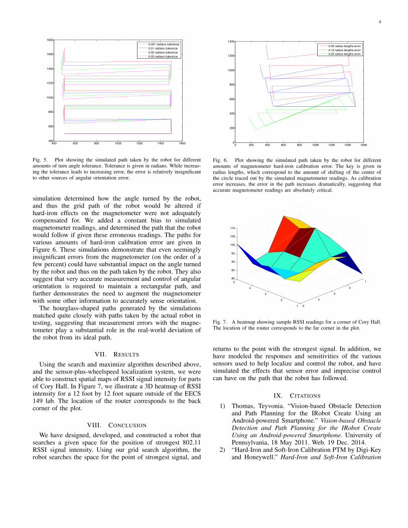
B. Effects of Varying Angle Tolerance on PathBecause our sensors took a significant amount of time to

update and because our software was unable to constantlymonitor sensor values, our finite state machine allowed fortransitions between the turning and driving forward states whenthe difference between the desired angle and the measuredangle was within a certain tolerance. In order to determine theeffect that threshold angles had on the robot’s traversal of thegrid path, we simulated the robot’s behavior for different turnthreshold angle values. The simulated paths are given belowin Figure 5. From the plot, it is clear that increasing angletolerance causes increasing errors in the angle turned by therobot, and thus increasing errors in the path taken by the robot.This simulation emphasizes the importance of writing softwarethat reads sensor values as often as possible, as the inabilityto do so leads to compounding errors in position.

C. Effects of Magnetometer Calibration Error on PathIn addition, we modeled the effects of errors in magne-

tometer calibration error on the path taken by the robot. This

4

400 600 800 1000 1200 1400 1600400

600

800

1000

1200

1400

1600

1800

0.001 radians tolerance0.01 radians tolerance0.02 radians tolerance0.03 radians tolerance

Student Version of MATLAB

Fig. 5. Plot showing the simulated path taken by the robot for differentamounts of turn angle tolerance. Tolerance is given in radians. While increas-ing the tolerance leads to increasing error, the error is relatively insignificantto other sources of angular orientation error.

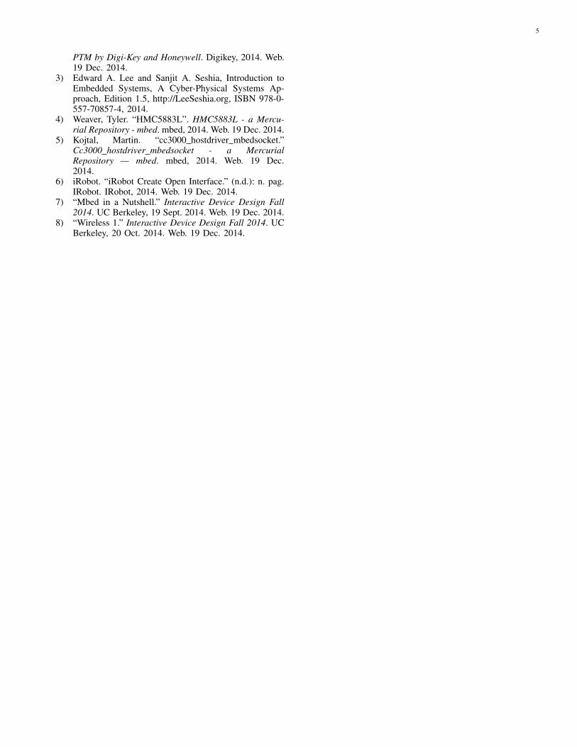
simulation determined how the angle turned by the robot,and thus the grid path of the robot would be altered ifhard-iron effects on the magnetometer were not adequatelycompensated for. We added a constant bias to simulatedmagnetometer readings, and determined the path that the robotwould follow if given these erroneous readings. The paths forvarious amounts of hard-iron calibration error are given inFigure 6. These simulations demonstrate that even seeminglyinsignificant errors from the magnetometer (on the order of afew percent) could have substantial impact on the angle turnedby the robot and thus on the path taken by the robot. They alsosuggest that very accurate measurement and control of angularorientation is required to maintain a rectangular path, andfurther demonstrates the need to augment the magnetometerwith some other information to accurately sense orientation.

The hourglass-shaped paths generated by the simulationsmatched quite closely with paths taken by the actual robot intesting, suggesting that measurement errors with the magne-tometer play a substantial role in the real-world deviation ofthe robot from its ideal path.

VII. RESULTS

Using the search and maximize algorithm described above,and the sensor-plus-wheelspeed localization system, we wereable to construct spatial maps of RSSI signal intensity for partsof Cory Hall. In Figure 7, we illustrate a 3D heatmap of RSSIintensity for a 12 foot by 12 foot square outside of the EECS149 lab. The location of the router corresponds to the backcorner of the plot.

VIII. CONCLUSION

We have designed, developed, and constructed a robot thatsearches a given space for the position of strongest 802.11RSSI signal intensity. Using our grid search algorithm, therobot searches the space for the point of strongest signal, and

0 200 400 600 800 1000 1200 1400 16000

200

400

600

800

1000

1200

1400

0.05 radius lengths error0.10 radius lengths error0.25 radius lengths error

Student Version of MATLAB

Fig. 6. Plot showing the simulated path taken by the robot for differentamounts of magnetometer hard-iron calibration error. The key is given inradius lengths, which correspond to the amount of shifting of the center ofthe circle traced out by the simulated magnetometer readings. As calibrationerror increases, the error in the path increases dramatically, suggesting thataccurate magnetometer readings are absolutely critical.

1

2

3

4

5 1

2

3

4

5

80

85

90

95

100

105

110

Student Version of MATLAB

Fig. 7. A heatmap showing sample RSSI readings for a corner of Cory Hall.The location of the router corresponds to the far corner in the plot.

returns to the point with the strongest signal. In addition, wehave modeled the responses and sensitivities of the varioussensors used to help localize and control the robot, and havesimulated the effects that sensor error and imprecise controlcan have on the path that the robot has followed.

IX. CITATIONS

1) Thomas, Teyvonia. “Vision-based Obstacle Detectionand Path Planning for the IRobot Create Using anAndroid-powered Smartphone.” Vision-based ObstacleDetection and Path Planning for the IRobot CreateUsing an Android-powered Smartphone. University ofPennsylvania, 18 May 2011. Web. 19 Dec. 2014.

2) “Hard-Iron and Soft-Iron Calibration PTM by Digi-Keyand Honeywell.” Hard-Iron and Soft-Iron Calibration

5

PTM by Digi-Key and Honeywell. Digikey, 2014. Web.19 Dec. 2014.

3) Edward A. Lee and Sanjit A. Seshia, Introduction toEmbedded Systems, A Cyber-Physical Systems Ap-proach, Edition 1.5, http://LeeSeshia.org, ISBN 978-0-557-70857-4, 2014.

4) Weaver, Tyler. “HMC5883L”. HMC5883L - a Mercu-rial Repository - mbed. mbed, 2014. Web. 19 Dec. 2014.

5) Kojtal, Martin. “cc3000 hostdriver mbedsocket.”Cc3000 hostdriver mbedsocket - a MercurialRepository — mbed. mbed, 2014. Web. 19 Dec.2014.

6) iRobot. “iRobot Create Open Interface.” (n.d.): n. pag.IRobot. IRobot, 2014. Web. 19 Dec. 2014.

7) “Mbed in a Nutshell.” Interactive Device Design Fall2014. UC Berkeley, 19 Sept. 2014. Web. 19 Dec. 2014.

8) “Wireless 1.” Interactive Device Design Fall 2014. UCBerkeley, 20 Oct. 2014. Web. 19 Dec. 2014.