Embed Size (px)
Citation preview

1
Review of di↵erential calculus
This chapter presents the main elements of di↵erential calculus needed in probabil-ity theory. Often, students taking a course on probability theory have problems withconcepts such as integrals and infinite series. In particular, the integration by partstechnique is recalled.
1.1 Limits and continuity
The first concept that we recall is that of the limit of a function, which is defined formallyas follows.
Definition 1.1.1. Let f be a real-valued function. We say that f(x) tends to f0 (2 R)as x tends to x0 if for any positive number ✏ there exists a positive number � such that
0 < |x� x0| < � =) |f(x)� f0| < ✏.
We write that limx!x0 f(x) = f0. That is, f0 is the limit of the function f(x) as x
tends to x0.
Remarks. (i) The function f(x) need not be defined at the point x0 for the limit to exist.(ii) It is possible that f(x0) exists, but f(x0) 6= f0.(iii) We write that lim
x!x0 f(x) = 1 if, for any M > 0 (as large as we want), thereexists a � > 0 such that
0 < |x� x0| < � =) f(x) > M.
Similarly for limx!x0
(iv) In the definition, x0
0 = ±1.actually be extended to the case when xis assumed to be a real number. However, the definition can
f(x) = �1.
and Technology, DOI: 10.1007/978-0-387-74995-2_1,© Springer Science + Business Media, LLC 2009
1M. Lefebvre, Basic Probability Theory with Applications, Springer Undergraduate Texts in Mathematics
2 1 Review of di↵erential calculus
Sometimes, we are interested in the limit of the function f(x) as x decreases orincreases to a given real number x0. The right-hand limit (resp., left-hand limit) of thefunction f(x) as x decreases (resp., increases) to x0 is denoted by lim
x#x0 f(x) [resp.,lim
x"x0 f(x)]. Some authors write limx!x
+0
f(x) [resp., limx!x
�0
f(x)]. If the limit off(x) as x tends to x0 exists, then
limx#x0
f(x) = limx"x0
f(x) = limx!x0
f(x).
Definition 1.1.2. The real-valued function f(x) is said to be continuous at the pointx0 2 R if (i) it is defined at this point, (ii) the limit as x tends to x0 exists, and (iii)lim
x!x0 f(x) = f(x0). If f is continuous at every point x0 2 [a, b] [or (a, b), etc.], thenf is said to be continuous on this interval.
Remarks. (i) In this textbook, a closed interval is denoted by [a, b], whereas (a, b) is anopen interval. We also have, of course, the intervals [a, b) and (a, b].(ii) If we rather write, in the definition, that the limit lim
x#x0 f(x) [resp., limx"x0 f(x)]
exists and is equal to f(x0), then the function is said to be right-continuous (resp., left-continuous) at x0. A function that is continuous at a given point x0 such that a < x0 < bis both right-continuous and left-continuous at that point.(iii) A function f is said to be piecewise continuous on an interval [a, b] if this intervalcan be divided into a finite number of subintervals on which f is continuous and hasright- and left-hand limits.(iv) Let f(x) and g(x) be two real-valued functions. The composition of the two functionsis denoted by g � f and is defined by
(g � f)(x) = g[f(x)].
A result used in Chapter 3 states that the composition of two continuous functions isitself a continuous function.
Example 1.1.1. Consider the function
u(x) =⇢
0 if x < 0,1 if x � 0, (1.1)
which is known as the Heaviside or unit step function. In probability, this functioncorresponds to the distribution function of the constant 1. It is also used to indicatethat the possible values of a certain random variable are the set of nonnegative realnumbers. For example, writing that
fX
(x) = e�xu(x) for all x 2 R
is tantamount to writing that

1.2 Derivatives 3
fX
(x) =⇢
0 if x < 0,e�x if x � 0,
where fX
(x) is called the density function of the random variable X.The function u(x) is defined for all x 2 R. In other contexts, u(0) is chosen di↵erently
as above. For instance, in some applications u(0) = 1/2. At any rate, the unit stepfunction is continuous everywhere, except at the origin, because (for us)
limx#0
u(x) = 1 and limx"0
u(x) = 0.
However, with the choice u(0) = 1, we may assert that u(x) is right-hand continuous atx = 0.
The previous definitions can be extended to the case of real-valued functions of two(or more) variables. In particular, the function f(x, y) is continuous at the point (x0, y0)if
limx! x0
y ! y0
f(x, y) = f( limx!x0
x, limy!y0
y).
This formula implies that the function f(x, y) is defined at (x0, y0) and that the limitof f(x, y) as (x, y) tends to (x0, y0) exists and is equal to f(x0, y0).
1.2 Derivatives
Definition 1.2.1. Suppose that the function f(x) is defined at x0 2 (a, b). If
f 0(x0) := limx!x0
f(x)� f(x0)x� x0
⌘ lim�x!0
f(x0 + �x)� f(x0)�x
exists, we say that the function f(x) is di↵erentiable at the point x0 and that f 0(x0)is the derivative of f(x) (with respect to x) at x0.
Remarks. (i) For the function f(x) to be di↵erentiable at x0, it must at least be con-tinuous at that point. However, this condition is not su�cient, as can be seen in theexample below.(ii) If the limit is taken as x # x0 (resp., x " x0) in the previous definition, then theresult (if the limit exists) is called the right-hand (resp., left-hand) derivative of f(x) atx0 and is sometimes denoted by f 0(x+
0 ) [resp., f 0(x�0 )]. If f 0(x0) exists, then f 0(x+0 ) =
f 0(x�0 ).(iii) The derivative of f at an arbitrary point x is also denoted by d
dx
f(x), or by Df(x).If we set y = f(x), then
f 0(x0) ⌘dy
dx
�
�
�
�
x=x0
.

4 1 Review of di↵erential calculus
(iv) If we di↵erentiate f 0(x), we obtain the second-order derivative of the function f ,denoted by f 00(x) or d
2
dx
2 f(x). Similarly, f 000(x) [or f (3)(x), or d
3
dx
3 f(x)] is the third-orderderivative of f , and so on.(v) One way to find the values of x that maximize or minimize the function f(x) isto calculate the first-order derivative f 0(x) and to solve the equation f 0(x) = 0. Iff 0(x0) = 0 and f 00(x0) < 0 [resp., f 00(x0) > 0], then f has a relative maximum (resp.,minimum) at x = x0. If f 0(x) 6= 0 for all x 2 R, we can check whether the function f(x)is always increasing or decreasing in the interval of interest.
Example 1.2.1. The function f(x) = |x| is continuous everywhere, but is not di↵eren-tiable at the origin, because we find that
f 0(x+0 ) = 1 and f 0(x�0 ) = �1.
Example 1.2.2. The function u(x) defined in Example 1.1.1 is obviously not di↵eren-tiable at x = 0, because it is not continuous at that point.
Example 1.2.3. The function
FX
(x) =
8
<
:
0 if x < 0,x if 0 x 1,1 if x > 1
is defined and continuous everywhere. It is also di↵erentiable everywhere, except atx = 0 and x = 1. We obtain that the derivative F 0
X
(x) of FX
(x), which is denoted byf
X
(x) in probability theory, is given by
fX
(x) =⇢
1 if 0 x 1,0 elsewhere.
Note that fX
(x) is discontinuous at x = 0 and x = 1. The function FX
(x) is an exampleof what is known in probability as a distribution function.Remark. Using the theory of distributions, we may write that the derivative of theHeaviside function u(x) is the Dirac delta function �(x) defined by
�(x) =⇢
0 if x 6= 0,1 if x = 0. (1.2)
The Dirac delta function is actually a generalized function. It is, by definition, such thatZ 1
�1�(x) dx = 1.
We also have, if f(x) is continuous at x = x0, that
1.2 Derivatives 5
Z 1
�1f(x)�(x� x0) dx = f(x0).
We do not recall the basic di↵erentiation rules, except that for the derivative of aquotient:
d
dx
f(x)g(x)
=g(x)f 0(x)� f(x)g0(x)
g2(x)if g(x) 6= 0.
Remark. Note that this formula can also be obtained by di↵erentiating the productf(x)h(x), where h(x) := 1/g(x).
Likewise, the formulas for calculating the derivatives of elementary functions areassumed to be known. However, a formula that is worth recalling is the so-called chainrule for derivatives.
Proposition 1.2.1. (Chain rule) Let the real-valued function h(x) be the compositefunction (g � f)(x). If f is di↵erentiable at x and g is di↵erentiable at the point f(x),then h is also di↵erentiable at x and
h0(x) = g0[f(x)]f 0(x).
Remark. If we set y = f(x), then the chain rule may be written as
d
dxg(y) =
d
dyg(y) · dy
dx= g0(y)f 0(x).
Example 1.2.4. Consider the function h(x) =p
x2 + 1. We may write that h(x) =(g � f)(x), with f(x) = x2 + 1 and g(x) =
px. We have:
g0(x) =1
2p
x=) g0[f(x)] =
12p
f(x)=
12p
x2 + 1.
Then,
f 0(x) = 2x =) h0(x) =1
2p
x2 + 1· (2x) =
xpx2 + 1
.
Finally, another useful result is known as l’Hospital’s rule.
Proposition 1.2.2. (L’Hospital’s rule) Suppose that
limx!x0
f(x) = limx!x0
g(x) = 0
or thatlim
x!x0f(x) = lim
x!x0g(x) = ±1.

6 1 Review of di↵erential calculus
If (i) f(x) and g(x) are di↵erentiable in an interval (a, b) containing the point x0, exceptperhaps at x0, and (ii) the function g(x) is such that g0(x) 6= 0 for all x 6= x0 in theinterval (a, b), then
limx!x0
f(x)g(x)
= limx!x0
f 0(x)g0(x)
holds. If the functions f 0(x) and g0(x) satisfy the same conditions as f(x) and g(x), wecan repeat the process. Moreover, the constant x0 may be equal to ±1.
Remark. If x0 = a or b, we can replace the limit as x ! x0 by lim x # a or lim x " b,respectively.
Example 1.2.5. In probability theory, one way of defining the density function fX
(x) ofa continuous random variable X is by calculating the limit of the ratio of the probabilitythat X takes on a value in a small interval about x to the length of this interval:
fX
(x) := lim✏#0
Probability that X 2 [x� (✏/2), x + (✏/2)]✏
.
The probability in question is actually equal to zero (in the limit as ✏ decreases to0). For example, we might have that {Probability that X 2 [x � (✏/2), x + (✏/2)]} =exp{�x + (✏/2)}� exp{�x� (✏/2)}, for x > 0 and ✏ small enough.
By making use of l’Hospital’s rule (with ✏ as variable), we find that
fX
(x) := lim✏#0
exp{�x + (✏/2)}� exp{�x� (✏/2)}✏
= lim✏#0
exp{�x + (✏/2)}(1/2)� exp{�x� (✏/2)}(�1/2)1
= exp{�x} for x > 0.
In two dimensions, we define the partial derivative of the function f(x, y) with respectto x by
@
@xf(x, y) ⌘ f
x
(x, y) = lim�x!0
f(x + �x, y)� f(x, y)�x
,
when the limit exists. The partial derivative of f(x, y) with respect to y is definedsimilarly. Note that even if the partial derivatives f
x
(x0, y0) and fy
(x0, y0) exist, thefunction f(x, y) is not necessarily continuous at the point (x0, y0). Indeed, the limit ofthe function f(x, y) must not depend on the way (x, y) tends to (x0, y0). For instance,let
f(x, y) =
8
>
<
>
:
xy
x2 + y2if (x, y) 6= (0, 0),
0 if (x, y) = (0, 0).(1.3)
Suppose that (x, y) tends to (0, 0) along the line y = kx, where k 6= 0. We then have:

1.3 Integrals 7
limx ! 0y ! 0
f(x, y) = limx!0
x(kx)x2 + (kx)2
=k
1 + k2(6= 0).
Therefore, we must conclude that the function f(x, y) is discontinuous at (0, 0). However,we can show that f
x
(0, 0) and fy
(0, 0) both exist (and are equal to 0).
1.3 Integrals
Definition 1.3.1. Let f(x) be a continuous (or piecewise continuous) function on theinterval [a, b] and let
I =n
X
k=1
f(⇠k
)(xk
� xk�1),
where ⇠k
2 [xk�1, xk
] for all k and a = x0 < x1 < · · · < xn�1 < x
n
= b is a partition ofthe interval [a, b]. The limit of I as n tends to 1, and x
k
� xk�1 decreases to 0 for all
k, exists and is called the (definite) integral of f(x) over the interval [a, b]. We write:
limn !1
(xk � xk�1) # 0 8k
I =Z
b
a
f(x) dx.
Remarks. (i) The limit must not depend on the choice of the partition of the interval[a, b].(ii) The function f(x) is called the integrand.(iii) If f(x) � 0 in the interval [a, b], then the integral of f(x) over [a, b] gives the areabetween the curve y = f(x) and the x-axis from a to b.(iv) If the interval [a, b] is replaced by an infinite interval, or if the function f(x) is notdefined or not bounded at at least one point in [a, b], then the integral is called improper.For example, we define the integral of f(x) over the interval [a,1) as follows:
Z 1
a
f(x) dx = limb!1
Z
b
a
f(x) dx.
If the limit exists, the improper integral is said to be convergent; otherwise, it is diver-gent. When [a, b] is the entire real line, we should write that
I1 :=Z 1
�1f(x) dx = lim
a!�1
Z 0
a
f(x) dx + limb!1
Z
b
0
f(x) dx
and not

8 1 Review of di↵erential calculus
I1 = limb!1
Z
b
�b
f(x) dx.
This last integral is actually the Cauchy principal value of the integral I1. The Cauchyprincipal value may exist even if I1 does not.
Definition 1.3.2. Let f(x) be a real-valued function. Any function F (x) such thatF 0(x) = f(x) is called a primitive (or indefinite integral or antiderivative) off(x).
Theorem 1.3.1. (Fundamental Theorem of Calculus) Let f(x) be a continuousfunction on the interval [a, b] and let F (x) be a primitive of f(x). Then,
Z
b
a
f(x) dx = F (b)� F (a).
Example 1.3.1. The function
fX
(x) =1
⇡(1 + x2)for x 2 R
is the density function of a particular Cauchy distribution. To obtain the average valueof the random variable X, we can calculate the improper integral
Z 1
�1xf
X
(x) dx =Z 1
�1
x
⇡(1 + x2)dx.
A primitive of the integrand g(x) := xfX
(x) is
G(x) =12⇡
ln(1 + x2).
We find that the improper integral diverges, because
lima!�1
Z 0
a
g(x) dx = lima!�1
[G(0)�G(a)] = �1
and
limb!1
Z
b
0
g(x) dx = limb!1
[G(b)�G(0)] =1.
Because 1 �1 is indeterminate, the integral indeed diverges. However, the Cauchyprincipal value of the integral is
limb!1
Z
b
�b
g(x) dx = limb!1
[G(b)�G(�b)] = limb!1
0 = 0.
There are many results on integrals that could be recalled. We limit ourselves tomentioning a couple of techniques that are helpful to find indefinite integrals or evaluatedefinite integrals.

1.3 Integrals 9
1.3.1 Particular integration techniques
(1) First, we remind the reader of the technique known as integration by substitution.Let x = g(y). We can write that
Z
f(x) dx =Z
f [g(y)]g0(y) dy.
This result actually follows from the chain rule. In the case of a definite integral, as-suming that(i) f(x) is continuous on the interval [a, b],(ii) the inverse function g�1(x) exists and(iii) g0(y) is continuous on [g�1(a), g�1(b)] (resp., [g�1(b), g�1(a)]) if g(y) is an increasing(resp., decreasing) function,we have:
Z
b
a
f(x) dx =Z
d
c
f [g(y)]g0(y) dy,
where a = g(c), c = g�1(a) and b = g(d), d = g�1(b).
Example 1.3.2. Suppose that we want to evaluate the definite integral
I2 :=Z 4
0
x�1/2ex
1/2dx.
Making the substitution x = g(y) = y2, so that y = g�1(x) = x1/2 (for x 2 [0, 4]), wecan write that
Z 4
0
x�1/2ex
1/2dx
y=x
1/2
=Z 2
0
y�1ey 2y dy = 2ey
�
�
�
�
2
0
= 2(e2 � 1).
Remark. If we are only looking for a primitive of the function f(x), then after havingfound a primitive of f [g(y)]g0(y) we must replace y by g�1(x) (assuming it exists) inthe function obtained. Thus, in the above example, we have:
Z
x�1/2ex
1/2dx =
Z
y�1ey 2y dy = 2ey = 2ex
1/2.
(2) Next, a very useful integration technique is based on the formula for the derivativeof a product:
d
dxf(x)g(x) = f 0(x)g(x) + f(x)g0(x).
Integrating both sides of the previous equation, we obtain:

10 1 Review of di↵erential calculus
f(x)g(x) =Z
f 0(x)g(x)dx +Z
f(x)g0(x)dx
()Z
f(x)g0(x) dx = f(x)g(x)�Z
f 0(x)g(x)dx.
Setting u = f(x) and v = g(x), we can write thatZ
udv = uv �Z
v du.
This technique is known as integration by parts. It is often used in probability tocalculate the moments of a random variable.
Example 1.3.3. To obtain the expected value of the square of a standard normal randomvariable, we can try to evaluate the integral
I3 :=Z 1
�1cx2e�x
2/2dx,
where c is a positive constant. When applying the integration by parts technique, onemust decide which part of the integrand to assign to u. Of course, u should be chosenso that the new (indefinite) integral is easier to find. In the case of I3, we set
u = cx and dv = xe�x
2/2dx.
Becausev =
Z
dv =Z
xe�x
2/2dx = �e�x
2/2,
it follows that
I3 = cx(�e�x
2/2)
�
�
�
�
1
�1+
Z 1
�1ce�x
2/2dx.
The constant c is such that the above improper integral is equal to 1 (see Chapter 3).Furthermore, making use of l’Hospital’s rule, we find that
limx!1
xe�x
2/2 = lim
x!1
x
ex
2/2
= limx!1
1ex
2/2 · x
= 0.
Similarly,lim
x!�1xe�x
2/2 = 0.
Hence, we may write that I3 = 0 + 1 = 1.Remarks. (i) Note that there is no elementary function that is a primitive of the func-tion e�x
2/2. Therefore, we could not have obtained a primitive (in terms of elementary
functions) of x2e�x
2/2 by proceeding as above.
1.3 Integrals 11
(ii) If we set u = ce�x
2/2 (and dv = x2dx) instead, then the resulting integral will be
more complicated. Indeed, we would have:
I3 = ce�x
2/2 x3
3
�
�
�
�
1
�1+
Z 1
�1cx4
3e�x
2/2dx =
Z 1
�1cx4
3e�x
2/2dx.
A particular improper integral that is important in probability theory is defined by
F (!) =Z 1
�1ej!xf(x)dx,
where j :=p�1 and ! is a real parameter, and where we assume that the real-valued
function f(x) is absolutely integrable; that is,Z 1
�1|f(x)|dx <1.
The function F (!) is called the Fourier transform (up to a constant factor) of thefunction f(x). It can be shown that
f(x) =12⇡
Z 1
�1e�j!xF (!)d!.
We say that f(x) is the inverse Fourier transform of F (!).In probability theory, a density function f
X
(x) is, by definition, nonnegative andsuch that
Z 1
�1f
X
(x)dx = 1.
Hence, the function F (!) is well defined. In this context, it is known as the characteristicfunction of the random variable X and is often denoted by C
X
(!). By di↵erentiatingit, we can obtain the moments of X (generally more easily than by performing theappropriate integrals).
Example 1.3.4. The characteristic function of a standard normal random variable is
CX
(!) = e�!
2/2.
We can show that the expected value of the square of X is given by
� d2
d!2e�!
2/2
�
�
�
�
!=0
= �e�!
2/2(!2 � 1)
�
�
�
�
!=0
= 1,
which agrees with the result found in the previous example.

12 1 Review of di↵erential calculus
Finally, to obtain the moments of a random variable X, we can also use its moment-generating function, which, in the continuous case, is defined (if the integral exists)by
MX
(t) =Z 1
�1etxf
X
(x)dx,
where we may assume that t is a real parameter. When X is nonnegative, the moment-generating function is actually the Laplace transform of the function f
X
(x).
1.3.2 Double integrals
In Chapter 4, on random vectors, we have to deal with double integrals to obtain variousquantities of interest. A joint density function is a nonnegative function f
X,Y
(x, y) suchthat
Z 1
�1
Z 1
�1f
X,Y
(x, y)dxdy = 1.
Double integrals are needed, in general, to calculate the probability P [A] that thecontinuous random vector (X, Y ) takes on a value in a given subset A of R2. We have:
P [A] =Z
A
Z
fX,Y
(x, y) dxdy.
One has to describe the region A with the help of functions of x or of y (whichever iseasier or more appropriate in the problem considered). That is,
P [A] =Z
b
a
Z
g2(x)
g1(x)
fX,Y
(x, y)dydx =Z
b
a
(
Z
g2(x)
g1(x)
fX,Y
(x, y)dy
)
dx (1.4)
or
P [A] =Z
d
c
Z
h2(y)
h1(y)
fX,Y
(x, y)dxdy =Z
d
c
(
Z
h2(y)
h1(y)
fX,Y
(x, y)dx
)
dy. (1.5)
Remarks. (i) If the functions g1(x) and g2(x) [or h1(y) and h2(y)] are constants, and ifthe function f
X,Y
(x, y) can be written as
fX,Y
(x, y) = fX
(x)fY
(y),
then the double integral giving P [A] can be expressed as a product of single integrals:
P [A] =Z
b
a
fX
(x)dx
Z
�
↵
fY
(y)dy,
where ↵ = g1(x) 8x and � = g2(x) 8x.
1.3 Integrals 13
(ii) Conversely, we can write the product of two single integrals as a double integral:Z
b
a
f(x)dx
Z
d
c
g(y)dy =Z
b
a
Z
d
c
f(x)g(y)dydx.
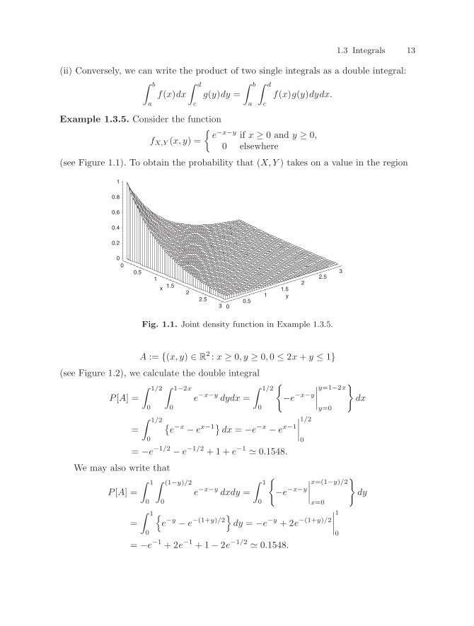
Example 1.3.5. Consider the function
fX,Y
(x, y) =⇢
e�x�y if x � 0 and y � 0,0 elsewhere
(see Figure 1.1). To obtain the probability that (X, Y ) takes on a value in the region
Fig. 1.1. Joint density function in Example 1.3.5.
A := {(x, y) 2 R2 : x � 0, y � 0, 0 2x + y 1}
(see Figure 1.2), we calculate the double integral
P [A] =Z 1/2
0
Z 1�2x
0
e�x�y dydx =Z 1/2
0
(
�e�x�y
�
�
�
�
y=1�2x
y=0
)
dx
=Z 1/2
0
�
e�x � ex�1
dx = �e�x � ex�1
�
�
�
�
1/2
0
= �e�1/2 � e�1/2 + 1 + e�1 ' 0.1548.
We may also write that
P [A] =Z 1
0
Z (1�y)/2
0
e�x�y dxdy =Z 1
0
(
�e�x�y
�
�
�
�
x=(1�y)/2
x=0
)
dy
=Z 1
0
n
e�y � e�(1+y)/2o
dy = �e�y + 2e�(1+y)/2
�
�
�
�
1
0
= �e�1 + 2e�1 + 1� 2e�1/2 ' 0.1548.
00.5
11.5
22.5
3
x
00.5
11.5
22.5
3
y
0
0.2
0.4
0.6
0.8
1

14 1 Review of di↵erential calculus
Remark. In this example, the functions gi
(x) and hi
(y), i = 1, 2, that appear in (1.4)and (1.5) are given by
g1(x) ⌘ 0, g2(x) = 1� 2x, h1(y) ⌘ 0 and h2(y) = (1� y)/2.
If B is the rectangle defined by
B = {(x, y) 2 R2 : 0 x 1, 0 y 2},
then we have:
P [B] =Z 2
0
Z 1
0
e�x�y dxdy =Z 1
0
e�x dx
Z 2
0
e�y dy
= �e�x
�
�
�
�
1
0
� e�y
�
�
�
�
2
0
= (1� e�1)(1� e�2) ' 0.5466.
1.4 Infinite series
Let a1, a2, . . . , an
, . . . be an infinite sequence of real numbers, where an
is given by acertain formula or rule, for example,
an
=1
n + 1for n = 1, 2, . . . .
We denote the infinite sequence by {an
}1n=1 or simply by {a
n
}. An infinite sequence issaid to be convergent if lim
n!1 an
exists; otherwise, it is divergent.Next, from the sequence {a
n
}1n=1 we define a new infinite sequence by
S1 = a1, S2 = a1 + a2, . . . , Sn
= a1 + a2 + · · · + an
, . . . .
Fig. 1.2. Integration region in Example 1.3.5.
2x+y = 1
2x+y < 1
0
0.2
0.4
0.6
0.8
1
0.1 0.2 0.3 0.4 0.5

1.4 Infinite series 15
Definition 1.4.1. The infinite sequence S1, S2, . . . , Sn
, . . . is represented byP1
n=1 an
and is called an infinite series. Moreover, Sn
:=P
n
k=1 ak
is called the nth partialsum of the series. Finally, if the limit lim
n!1 Sn
exists (resp., does not exist), we saythat the series is convergent (resp., divergent).
In probability, the set of possible values of a discrete random variable X may befinite or countably infinite (see p. 27). In the latter case, the probability function p
X
ofX is such that
1X
k=1
pX
(xk
) = 1,
where x1, x2, . . . are the possible values of X. In the most important cases, the possiblevalues of X are actually the integers 0, 1, . . . .
1.4.1 Geometric series
A particular type of infinite series encountered in Chapter 3 is known as a geometricseries. These series are of the form
1X
n=1
arn�1 or1X
n=0
arn, (1.6)
where a and r are real constants.
Proposition 1.4.1. If |r| < 1, the geometric series S(a, r) :=P1
n=0 arn converges toa/(1� r). If |r| � 1 (and a 6= 0), then the series is divergent.
To prove the above results, we simply have to consider the nth partial sum of theseries:
Sn
=n
X
k=1
ark�1 = a + ar + ar2 + · · · + arn�1.
We have:rS
n
= ar + ar2 + ar3 + · · · + arn�1 + arn,
so thatS
n
� rSn
= a� arn
r 6=1=) Sn
=a(1� rn)
1� r.
Hence, we deduce that
S := limn!1
Sn
=
( a
1� rif |r| < 1,
does not exist if |r| > 1.
If r = 1, we have that Sn
= na, so that the series diverges (if a 6= 0). Finally, we canshow that the series is also divergent if r = �1.

16 1 Review of di↵erential calculus
Other useful formulas connected with geometric series are the following: if |r| < 1,then
1X
k=1
ark =ar
1� r
and1X
k=0
ak rk =ar
(1� r)2. (1.7)
In probability, we also use power series, that is, series of the form
S(x) := a0 + a1x + a2x2 + · · · + an
xn + · · · ,
where ak
is a constant, for k = 0, 1 . . . . In particular, we use the fact that it is possibleto express functions, for instance, the exponential function ecx, as a power series:
ecx = 1 + cx +c2
2!x2 + · · · +
cn
n!xn + · · · for all x 2 R. (1.8)
This power series is called the series expansion of ecx.Remark. Note that a geometric series S(a, r) is a power series S(r) for which all theconstants a
k
are equal to a.In general, a power series converges for all values of x in an interval around 0. If
a given series expansion is valid for |x| < R (> 0), we say that R is the radius ofconvergence of the series. For |x| < R, the series can be di↵erentiated and integratedterm by term:
S0(x) = a1 + 2a2x + · · · + nan
xn�1 + · · · (1.9)
andZ
x
0
S(t) dt = a0x + a1x2
2+ · · · + a
n
xn+1
n + 1+ · · · .
The interval of convergence of a power series having a radius of convergence R > 0 isat least (�R,R). The series may or may not converge for x = �R and x = R. Because
S(0) = a0 2 R,
any power series converges for x = 0. If the series does not converge for any x 6= 0, wewrite that R = 0. Conversely, if the series converges for all x 2 R, then R =1.
To calculate the radius of convergence of a power series, we can make use ofd’Alembert’s ratio test: suppose that the limit
L := limn!1
�
�
�
�
un+1
un
�
�
�
�
(1.10)
exists. Then, the seriesP1
n=0 un

1.4 Infinite series 17
(a) converges absolutely if L < 1;(b) diverges if L > 1.
Remarks. (i) If the limit L in (1.10) does not exist, or if L = 1, then the test is incon-clusive. There exist other criteria that can be used, for instance, Raabe’s test.(ii) An infinite series
P1n=0 u
n
converges absolutely ifP1
n=0 |un
| converges. A series thatconverges absolutely is also convergent.(iii) In the case of a power series, we calculate
limn!1
�
�
�
�
an+1xn+1
an
xn
�
�
�
�
= limn!1
�
�
�
�
an+1
an
�
�
�
�
|x|.
For example, the series expansion of the exponential function ecx given in (1.8) is validfor all x 2 R. Indeed, a
n
= cn/n!, so that
limn!1
�
�
�
�
an+1xn+1
an
xn
�
�
�
�
= limn!1
�
�
�
�
c
n + 1
�
�
�
�
|x| = 0 < 1 8x 2 R.
Example 1.4.1. To obtain the mean of a geometric random variable, we can computethe infinite sum
1X
k=1
k(1� p)k�1p =p
1� p
1X
k=0
k(1� p)k
(1.7)=
p
1� p
1� p
p2=
1p,
where 0 < p < 1. To prove Formula (1.7), we can use (1.9).
Example 1.4.2. A Poisson random variable is such that its probability function is givenby
pX
(x) = e��
�x
x!for x = 0, 1, . . . ,
where � is a positive constant. We have:
1X
x=0
pX
(x) =1X
x=0
e��
�x
x!= e��
1X
x=0
�x
x!(1.8)= e��e� = 1,
as required.
Example 1.4.3. The power series
Sk
(x) := 1 + kx +k(k � 1)
2!x2 + · · · +
k(k � 1)(k � 2) · · · (k � n + 1)n!
xn + · · ·
is the series expansion of the function (1 + x)k, and is called the binomial series. Inprobability, k will be a natural integer. It follows that the series has actually a finitenumber of terms and thus converges for all x 2 R. Moreover, we can then write that

18 1 Review of di↵erential calculus
k(k � 1)(k � 2) · · · (k � n + 1)n!
=k!
(k � n)!n!
for n = 1, . . . , k.
To conclude this review of calculus, we give the main logarithmic formulas:
ln ab = ln a + ln b; ln a/b = ln a� ln b; ln ab = b ln a.
We also have:ln ecx = eln(cx) = cx
andef(x) ln x = xf(x).
1.5 Exercises for Chapter 1
Solved exercises1
Question no. 1Calculate lim
x#0 x sin(1/x).
Question no. 2For what values of x is the function
f(x) =
8
>
<
>
:
sinx
xif x 6= 0,
1 if x = 0
continuous?
Question no. 3Di↵erentiate the function f(x) =
p3x + 1(2x2 + 1)2.
Question no. 4Find the limit lim
x#0 x lnx.
Question no. 5Evaluate the definite integral
I5 :=Z
e
1
lnx
xdx.
1 The solutions can be found in Appendix C.

1.5 Exercises for Chapter 1 19
Question no. 6Find the value of the definite integral
I6 :=Z 1
�1x3e�x
2/2dx.
Question no. 7Find the Fourier transform of the function
f(x) = ce�cx for x � 0,
where c is a positive constant.
Question no. 8Let
f(x, y) =⇢
x + y if 0 x 1, 0 y 1,0 elsewhere.
CalculateI8 :=
Z
A
Z
f(x, y) dxdy,
where A := {(x, y) 2 R2 : 0 x 1, 0 y 1, x2 < y} (see Figure 1.3).
Fig. 1.3. Region A in solved exercise no. 8.
Question no. 9Find the value of the infinite series
S9 :=18
+116
+132
+ · · · .
A
0
0.2
0.4
0.6
0.8
1
0.2 0.4 0.6 0.8 1
20 1 Review of di↵erential calculus
Question no. 10Calculate
S10 :=1X
k=1
k2(1� p)k�1p,
where 0 < p < 1.
Exercises
Question no. 1Let
F (x) =
8
<
:
0 if x < 0,1/2 if x = 0,
1� (1/2)e�x if x > 0.
Calculate (a) limx"0 F (x), (b) lim
x#0 F (x), and (c) limx!0 F (x).
Question no. 2Consider the function
F (x) =
8
>
>
<
>
>
:
0 if x < 0,1/3 if 0 x < 1,2/3 if 1 x < 2,1 if x � 2.
For what values of x is F (x) left-continuous? right-continuous? continuous?
Question no. 3Find the limit as x tends to 0 of the function
f(x) =x2 sin(1/x)
sinxfor x 2 R.
Question no. 4Is the function
f(x) =⇢
e1/x if x 6= 0,0 if x = 0
continuous or discontinuous at x = 0? Justify.
Question no. 5Find the fourth-order derivative of the function F (!) = e�!
2/2, for any ! 2 R, and
evaluate the derivative at ! = 0.

1.5 Exercises for Chapter 1 21
Question no. 6Find the following limit:
lim✏#0
�
1 + x� ✏
2
�
e�x+(✏/2) ��
1 + x + ✏
2
�
e�x�(✏/2)
✏.
Question no. 7Determine the second-order derivative of f(x) = 3
p2x2.
Question no. 8Calculate the derivative of
f(x) = 1 + 3p
x2 for x 2 R
and find the value of x that minimizes this function.
Question no. 9Use the fact that
Z 1
0
xn�1e�xdx = (n� 1)! for n = 1, 2, . . .
to evaluate the integralZ 1
0
xn�1e�cxdx,
where c is a positive constant.
Question no. 10Use the following formula:
Z 1
�1e�(x�m)2/2dx =
p2⇡,
where m is a real constant, to calculate the definite integralZ 1
�1x2e�x
2/2dx.
Question no. 11Evaluate the improper integral
Z 1
0
e�x
xdx.
22 1 Review of di↵erential calculus
Question no. 12Find a primitive of the function
f(x) = e�x sinx for x 2 R.
Question no. 13Find the Fourier transform of the function
f(x) =c
2e�c|x| for x 2 R,
where c is a positive constant.
Question no. 14Let
f(x, y) =⇢
32x if 1 x 2, 1 y 2, x y,0 elsewhere.
Calculate the double definite integralZ
A
Z
f(x, y) dxdy,
whereA := {(x, y) 2 R2 : 1 x 2, 1 y 2, x2 < y}.
Question no. 15The convolution of two functions, f and g, is denoted by f ⇤ g and is defined by
(f ⇤ g)(x) =Z 1
�1f(y)g(x� y) dy.
Letf(x) =
⇢
ce�cx if x � 0,0 if x < 0,
where c is a positive constant, and assume that g(x) ⌘ f(x) (i.e., g is identical to f).Find (f ⇤ g)(x).Remark. In probability theory, the convolution of f
X
and fY
is the probability densityfunction of the sum Z := X+Y of the independent random variables X and Y . The resultof the above exercise implies that the sum of two independent exponentially distributedrandom variables with the same parameter c has a gamma distribution with parameters↵ = 2 and � = c.

1.5 Exercises for Chapter 1 23
Question no. 16Prove that
I :=Z 1
�1
1p2⇡
e�z
2/2dz = 1
by first writing that
I2 =12⇡
Z 1
�1e�z
2/2dz
Z 1
�1e�w
2/2dw =
12⇡
Z 1
�1
Z 1
�1e�(z2+w
2)/2dzdw
and then using polar coordinates. That is, set z = r cos ✓ and w = r sin ✓ (with r � 0),so that
r =p
z2 + w2 and ✓ = tan�1(w/z).
Remark. We find that I2 = 1. Justify why this implies that I = 1 (and not I = �1).
Question no. 17Determine the value of the infinite series
12!
x2 � 13!
x3 + · · · +(�1)n
n!xn + · · · .
Question no. 18Let
S(q) =1X
n=1
qn�1,
where 0 < q < 1. CalculateZ 1/2
0
S(q)dq.
Question no. 19(a) Calculate the infinite series
M(t) :=1X
k=0
etke�↵
↵k
k!,
where ↵ > 0.(b) Evaluate the second-order derivative M 00(t) at t = 0.Remark. The function M(t) is the moment-generating function of a random variable Xhaving a Poisson distribution with parameter ↵. Moreover, M 00(0) gives us the expectedvalue of X2.

24 1 Review of di↵erential calculus
Question no. 20(a) Determine the value of the power series
G(z) :=1X
k=0
zk (1� p)kp,
where z 2 R and p 2 (0, 1) are such that |z| < (1� p)�1.(b) Calculate
dk
dzk
G(z) for k = 0, 1, . . .
at z = 0.Remark. The function G
X
(z) :=P1
k=0 zkpX
(k) is called the generating function of thediscrete random variable X taking its values in the set {0, 1, . . .} and having probabilitymass function p
X
(k). Furthermore,
1k!
dk
dzk
GX
(z)�
�
�
�
z=0
yields pX
(k).
Multiple choice questions
Question no. 1Calculate the limit
limx!1
px� 1
1� x.
(a) �1 (b) �1/2 (c) 1/2 (d) 1 (e) does not exist
Question no. 2Let u(x) be the Heaviside function (see p. 2) and define h(x) = eu(x)/2, for x 2 R.
Calculate the limit of the function h(x) as x tends to 0.(a) 1/2 (b) 1 (c) (1 + e1/2)/2 (d) e1/2 (e) does not exist
Question no. 3Evaluate the second-order derivative of the function
F (!) =2(2 + j!)(4 + !2)
for ! 2 R
at ! = 0.a) �1/4 (b) �1/2 (c) 0 (d) 1/4 (e) 1/2

1.5 Exercises for Chapter 1 25
Question no. 4Find the following limit:
limx!1
✓
1 +1x
◆
x
.
Indication. Take the natural logarithm of the expression first and then use the fact thatlnx is a continuous function.(a) 0 (b) 1 (c) e (d) 1 (e) does not exist
Question no. 5Use the formula
Z 1
�1
1p2⇡b
exp⇢
� (x� a)2
2b2
�
dx = 1,
where a and b (> 0) are constants, to evaluate the definite integralZ 1
0
1p2⇡
e�2x
2dx.
(a) 1/4 (b) 1/2 (c) 1 (d) 2 (e) 4
Question no. 6Calculate the definite integral
Z 1
0
x lnxdx.
(a) �1 (b) �1 (c) �1/2 (d) �1/4 (e) 0
Question no. 7Suppose that
f(x) =⇢
1 if 0 x 1,0 elsewhere
and that g(x) = f(x) for all x 2 R. Find (f ⇤ g)(3/2), where ⇤ denotes the convolutionof f and g (see no. 15, p. 22).(a) 0 (b) 1/2 (c) 1 (d) 3/2 (e) 2
Question no. 8Let
f(x, y) =⇢
2� x� y if 0 < x < 1, 0 < y < 1,0 elsewhere.
Calculate the following double integral:Z
A
Z
f(x, y) dxdy,

26 1 Review of di↵erential calculus
whereA := {(x, y) 2 R2 : 0 < x < 1, 0 < y < 1, x + y > 1}.
(a) 1/6 (b) 1/4 (c) 1/3 (d) 1/2 (e) 5/6
Question no. 9Find the value of the natural logarithm of the infinite product
1Y
n=1
e1/2n
= e1/2 ⇥ e1/4 ⇥ e1/8 ⇥ · · · .
(a) �1 (b) �1/2 (c) 0 (d) 1/2 (e) 1
Question no. 10We define a0 = 0 and
ak
= e�c
c|k|
2|k|! for k = . . . ,�2,�1, 1, 2, . . . ,
where c > 0 is a constant. Find the value of the infinite seriesP1
k=�1 ak
.(a) 1� e�c (b) 0 (c) 1 (d) (1/2)e�c (e) 1 + e�c