MA20010: Vector Calculus and PartialDifferential Equations

Robert Scheichl

Department of Mathematical SciencesUniversity of Bath

October 2006 – January 2007

This course deals with

basic concepts and results in vector integration and vector calculus, Fourier series, andthe solution of partial differential equations by separation of variables.

It is

fundamental to most areas of applied Maths and many areas of pure Maths,

a prerequisite for a large number (11!!) of courses in Semester 2 and in Year 3/4.

There will be two class tests:

Tuesday, 31st October, 5.15pm (Line, surface, volume integrals)

Tuesday, 28th November, 5.15pm (Vector calculus and integral theorems)

Questions will be similar to the questions on the problem sheets!

Please take this course seriously and do not fall behind with the problemsheets. The syllabus for this course is very dense and only through constant practicewill you be able to grasp the multitude of methods and concepts.

Please revise

MA10005 Sect. 6-8 Multivariate Calculus

MA10006 Sect. 1 Vector Algebra

The first AIM quiz is designed to help you focus on the relevant material in those courses.

Contents

1 Vector Integration 11.1 Line Integrals . . . . . . . . . . . . . . . . . . . . . . . . . . . . . . . . . . . . . 1

1.1.1 Parametric Representation – Arclength . . . . . . . . . . . . . . . . . . . 31.1.2 Line Integrals of Scalar Fields . . . . . . . . . . . . . . . . . . . . . . . . 51.1.3 Line Integrals of Vector Fields . . . . . . . . . . . . . . . . . . . . . . . . 61.1.4 Application to Particle Motion . . . . . . . . . . . . . . . . . . . . . . . . 8

1.2 Surface Integrals . . . . . . . . . . . . . . . . . . . . . . . . . . . . . . . . . . . 91.2.1 The Surface Elements dS and dS . . . . . . . . . . . . . . . . . . . . . . 101.2.2 Surface Integrals of Scalar Fields . . . . . . . . . . . . . . . . . . . . . . 121.2.3 Flux – Surface Integrals of Vector Fields . . . . . . . . . . . . . . . . . . 13

1.3 Volume Integrals . . . . . . . . . . . . . . . . . . . . . . . . . . . . . . . . . . . 151.3.1 Change of Variables – Reparametrisation . . . . . . . . . . . . . . . . . . 16

2 Vector Calculus 202.1 Directional Derivatives and Gradients . . . . . . . . . . . . . . . . . . . . . . . . 20

2.1.1 Application: Level Surfaces and Grad . . . . . . . . . . . . . . . . . . . . 222.2 Divergence and Curl; the ∇–Operator . . . . . . . . . . . . . . . . . . . . . . . . 22

2.2.1 Second order derivatives – the Laplace Operator . . . . . . . . . . . . . . 232.2.2 Application: Potential Theory [Bourne, pp. 225–243] . . . . . . . . . . . 24

2.3 Differentiation in Curvilinear Coordinates . . . . . . . . . . . . . . . . . . . . . 252.3.1 Orthogonal Curvilinear Coordinates . . . . . . . . . . . . . . . . . . . . . 252.3.2 Grad, div, curl, ∇2 in Orthogonal Curvilinear Coordinates . . . . . . . . 27

3 Integral Theorems 303.1 The Divergence Theorem of Gauss . . . . . . . . . . . . . . . . . . . . . . . . . 313.2 Green’s Theorem in the Plane . . . . . . . . . . . . . . . . . . . . . . . . . . . . 333.3 Stokes’ Theorem . . . . . . . . . . . . . . . . . . . . . . . . . . . . . . . . . . . 34

4 Fourier Series 364.1 Periodicity of Fourier Series . . . . . . . . . . . . . . . . . . . . . . . . . . . . . 394.2 Fourier Convergence . . . . . . . . . . . . . . . . . . . . . . . . . . . . . . . . . 404.3 Gibbs’ Phenomenon . . . . . . . . . . . . . . . . . . . . . . . . . . . . . . . . . . 414.4 Half-range Series . . . . . . . . . . . . . . . . . . . . . . . . . . . . . . . . . . . 424.5 Application: Eigenproblems for 2nd-order ODEs . . . . . . . . . . . . . . . . . . 43

5 Partial Differential Equations 465.1 Classification of Partial Differential Equations . . . . . . . . . . . . . . . . . . . 465.2 Separation of Variables – Fourier’s Method . . . . . . . . . . . . . . . . . . . . . 47

5.2.1 Elliptic PDEs – Laplace’s Equation . . . . . . . . . . . . . . . . . . . . . 47

2

5.2.2 Circular Geometry . . . . . . . . . . . . . . . . . . . . . . . . . . . . . . 515.2.3 Hyperbolic PDEs – Wave Equation . . . . . . . . . . . . . . . . . . . . . 535.2.4 Parabolic PDEs – Diffusion Equation . . . . . . . . . . . . . . . . . . . . 56

5.3 Other Solution Methods for PDEs (not examinable!) . . . . . . . . . . . . . 565.3.1 The Laplace Transform Method . . . . . . . . . . . . . . . . . . . . . . . 565.3.2 D’Alembert’s Solution of the Wave Equation . . . . . . . . . . . . . . . . 58

Chapter 1

Vector Integration

In this course we will be dealing with functions in more than one unknown whose functionvalue might be vector–valued as well.

Definition 1.1. A function F : Rn → R

n is called a vector field on Rn. A function

f : Rn → R is called a scalar field on R

n. (Usually n will be 2 or 3.)

Example 1.2. Typical examples of vector fields are

• gravitational field G(x)

• electrical field E(x)

• magnetic field B(x)

• velocity field V (x)

Example 1.3. Typical examples of scalar fields are

• speed |V (x)|

• kinetic energy 1

2m |V (x)|2

• electrical potential ϕE(x)

We will now learn how to integrate such fields in Rn.

1.1 Line Integrals [Bourne, pp 147–156] & [Anton, pp. 1100–1123]

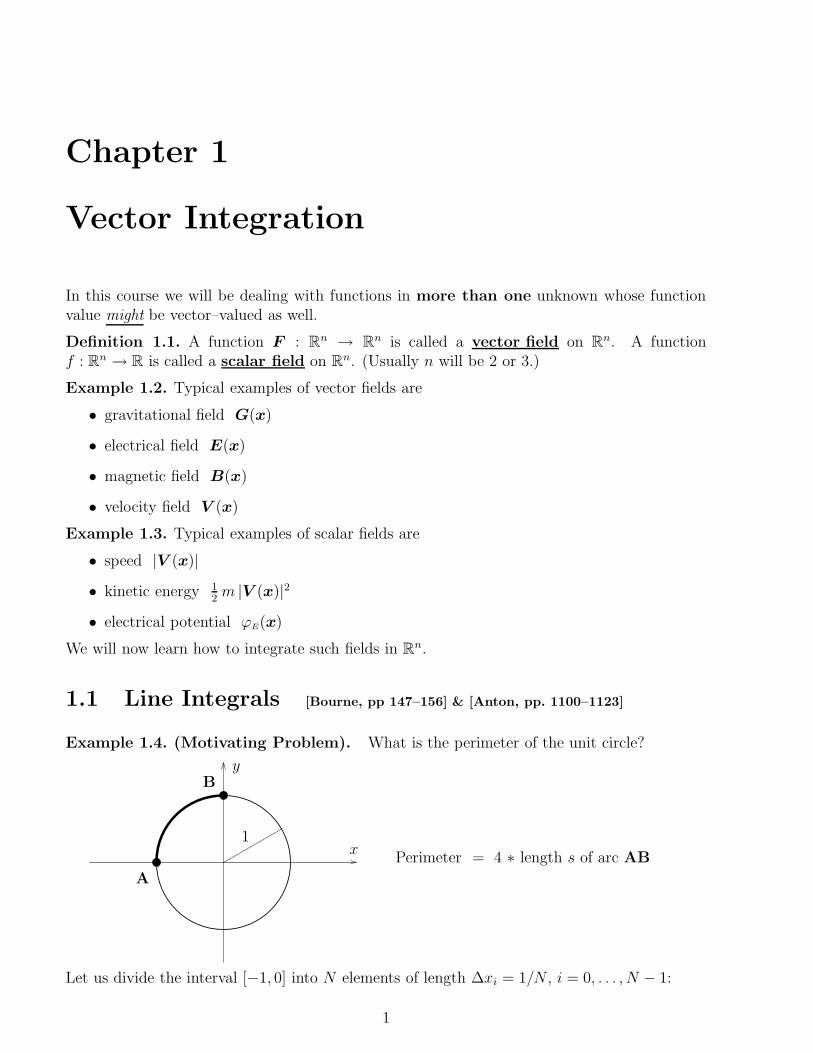
Example 1.4. (Motivating Problem). What is the perimeter of the unit circle?

PSfrag replacements 1x

y

A

B

Perimeter = 4 ∗ length s of arc AB

Let us divide the interval [−1, 0] into N elements of length ∆xi = 1/N , i = 0, . . . , N − 1:

1

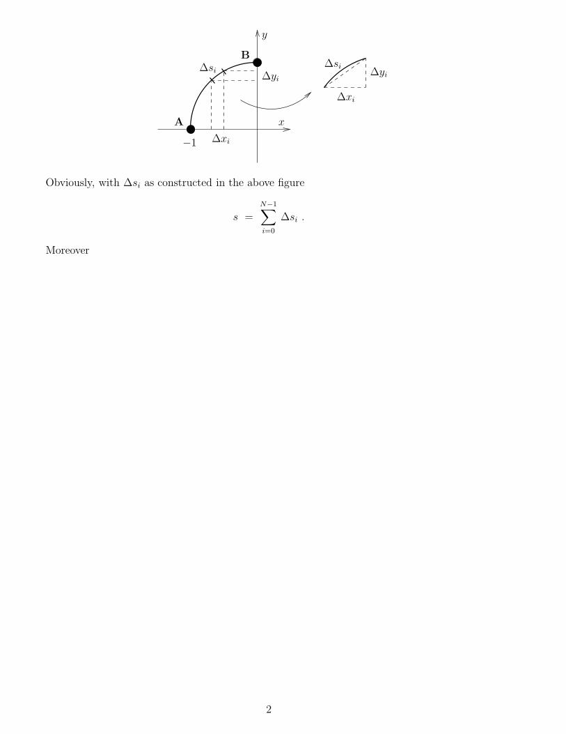
PSfrag replacements

−1

x

y

∆xi

∆xi

∆yi∆yi

∆si∆si

A

B

Perimeter = 4 ∗ length s of arc AB

Obviously, with ∆si as constructed in the above figure

s =N−1∑

i=0

∆si .

Moreover

2

s =

∫ 0

−1

1√1 − x2

dx (1.1)

DIY Use the substitution x = − cos θ to evaluate (1.1):

Hence, the perimeter is . . . . . . . . . . . . . . .

1.1.1 Parametric Representation – Arclength

Let C be a curve in Rn with parametric representation r(t), i.e.

C = r(t) : t0 ≤ t ≤ te (1.2)

where r : [t0, te] → Rn is continuously differentiable.

PSfrag replacements

0

C

r(t)

As t increases r(t) traces out the curve C.

Note. In Ex. 1.4 t was chosen to be x. In general, t can be any parameter (e.g. angle θ).

3

Example 1.5. Give a parametric representation of the ellipsex2

a2+

y2

b2= 1.

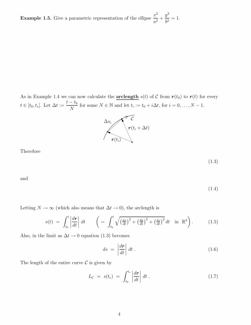
As in Example 1.4 we can now calculate the arclength s(t) of C from r(t0) to r(t) for every

t ∈ [t0, te]. Let ∆t :=t − t0

Nfor some N ∈ N and let ti := t0 + i∆t, for i = 0, . . . , N − 1.

PSfrag replacements C

r(ti)

r(ti + ∆t)

∆si

Therefore

(1.3)

and

(1.4)

Letting N → ∞ (which also means that ∆t → 0), the arclength is

s(t) =

∫ t

t0

∣

∣

∣

∣

dr

dt

∣

∣

∣

∣

dt

(

=

∫ t

t0

√

(

dxdt

)2+

(

dy

dt

)2+

(

dzdt

)2dt in R

3

)

. (1.5)

Also, in the limit as ∆t → 0 equation (1.3) becomes

ds =

∣

∣

∣

∣

dr

dt

∣

∣

∣

∣

dt . (1.6)

The length of the entire curve C is given by

LC = s(te) =

∫ te

t0

∣

∣

∣

∣

dr

dt

∣

∣

∣

∣

dt . (1.7)

4

1.1.2 Line Integrals of Scalar Fields

Now assume we want to calculate the integral of a scalar field f : Rn → R along the curve C.

Geometrically this means, to calculate the following area A:PSfrag replacements

C

A

x

y

z

r(t0)

r(te)

f(r(ti))

z = f(x, y)

∆si

(in R2)

As in (1.4) with ∆t =te − t0

Nwe get

(i.e. we approximate the area by the sum of the strips.)

Hence for N → ∞A =

∫ te

t0

f(r(t))

∣

∣

∣

∣

dr

dt

∣

∣

∣

∣

dt

(an ordinary integral of a scalar valued function of t).

Definition 1.6. The line integral of a scalar field f : Rn → R along the curve C in (1.2)

is defined as∫

C

f ds :=

∫ te

t0

f(r(t))

∣

∣

∣

∣

dr

dt

∣

∣

∣

∣

dt . (1.8)

Remark 1.7.

(a) The value of∫

Cf ds does not depend on the choice of parametrisation, even if the orien-

tation of C is reversed [Bourne, p. 148], [Anton, pp. 1108–1109].

(b) The length of the curve C in (1.6) is a special line integral, i.e. LC =∫

C1 ds.

Example 1.8. Integrate f(x, y) = 2xy around the first quadrant of a circle with radius a asshown:

PSfrag replacements

ax

y

5

Step 1. Parametrise circle:

Step 2. Calculate the line element ds :

DIY Step 3. Apply formula (1.8) for the line integral:

1.1.3 Line Integrals of Vector Fields

Definition 1.9. The work integral of a vector field F : Rn → R

n along the curve C in(1.2) is defined as

∫

C

F · dr :=

∫ te

t0

F (r(t)) · dr

dtdt . (1.9)

(dot product!)

Theorem 1.10. If T is the unit tangent vector to C in (1.2) that points in the direction inwhich t is increasing, then

∫

C

F · dr =

∫

C

(F · T ) ds , (1.10)

i.e. the work integral of F = the line integral of the component of F parallel to C.

Proof.

6

Remark 1.11.

(a) It follows directly from Theorem 1.10 that a reversal of the orientation of C does changethe sign of the work integral (in contrast to the line integral of a scalar field, cf. Remark1.7(a)) [Bourne, p. 153], [Anton, p. 1109].

(b) If F is a force field then∫

CF · dr is the work done by moving a particle from r(t0) to

r(te) along the curve C; hence the term work integral.

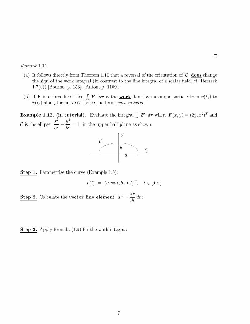
Example 1.12. (in tutorial). Evaluate the integral∫

CF · dr where F (x, y) = (2y, x2)T and

C is the ellipsex2

a2+

y2

b2= 1 in the upper half plane as shown:

PSfrag replacements

x

y

C

a

b

Step 1. Parametrise the curve (Example 1.5):

r(t) = (a cos t, b sin t)T , t ∈ [0, π].

Step 2. Calculate the vector line element dr =dr

dtdt :

Step 3. Apply formula (1.9) for the work integral:

7

Definition 1.13. (in tutorial). Let F be a vector field such that F = F1i+F2j +F3k. The(vector valued) integrals

∫

CF ds and

∫

CF ∧ dr are defined as

∫

C

F ds :=

(∫

C

F1 ds,

∫

C

F2 ds,

∫

C

F3 ds

)T

∫

C

F ∧ dr :=

∫ te

t0

F (r(t)) ∧ dr

dtdt .

Definition 1.14. A vector field F : Rn → R

n is called conservative, if∫

C1

F · dr =

∫

C2

F · dr (1.11)

for any two curves C1 and C2 connecting two points x0 and xe in Rn

PSfrag replacements

x0

xe

C1

C2

1.1.4 Application to Particle Motion

Suppose F : Rn → R

n is a force field and suppose that a particle of mass m moves along acurve C through this field. Suppose further that r(t) is the position of the particle at timet ∈ [t0, te] (i.e. r(t) is a parametric representation of C where the parameter t is time).

Recall:

• particle velocity V (t) =dr

dt

• kinetic energy K(t) = 1

2m |V (t)|2

Newton’s Second Law states

Force applied = mass * acceleration =⇒ F (r(t)) = md2r

dt2.

Therefore∫

C

F · dr =

∫ te

t0

F (r(t)) · dr

dtdt =

∫ te

t0

(

md2r

dt2

)

· dr

dtdt

=1

2m

∫ te

t0

d

dt

(

dr

dt· dr

dt

)

dt =1

2m

∫ te

t0

d

dt|V (t)|2 dt

and so by the Fundamental Theorem of Calculus∫

C

F · dr =1

2m |V (te)|2 − 1

2m |V (t0)|2 , (1.12)

or in other words

8

Work done = Change in kinetic energy from t0 to te

(“conservation of energy principle”).

1.2 Surface Integrals [Bourne, pp. 172–189] & [Anton, pp. 1130–1145]

In the previous section we discussed integrals along “one-dimensional” curves in Rn. Now we

want to look at integrals on two-dimensional surfaces in Rn.

You have already done the case n = 2 in MA10005, i.e. (flat) surfaces in R2. Now we will

consider surfaces in R3, i.e. n = 3.

Recall (for curves): parametric representationPSfrag replacements

t0 te

C

r(t)

Now, let S be a (two-dimensional) surface in R3 with parametric representation r(u, v), i.e.

S = r(u, v) : (u, v) ∈ D (1.13)

where r : D → R3 is continuously differentiable and D ⊂ R

2.

Example 1.15. (Step 1). A cylindrical shell of height b and radius a

PSfrag replacements

x

y

z

uu

v

v

a

b

b

2π

D

r(u, v)

parametric representation

can be parametrised by

9

1.2.1 The Surface Elements dS and dS

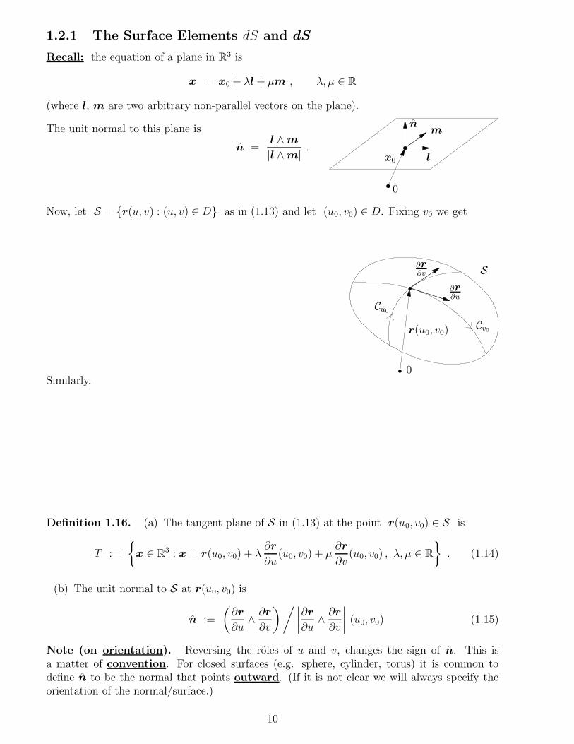
Recall: the equation of a plane in R3 is

x = x0 + λl + µm , λ, µ ∈ R

(where l, m are two arbitrary non-parallel vectors on the plane).

The unit normal to this plane is

n =l ∧ m

|l ∧ m| .

PSfrag replacements

l

mn

x0

0

Now, let S = r(u, v) : (u, v) ∈ D as in (1.13) and let (u0, v0) ∈ D. Fixing v0 we get

PSfrag replacements

r(u0, v0)

∂r∂u

∂r∂v

Cu0

Cv0

S

0Similarly,

Definition 1.16. (a) The tangent plane of S in (1.13) at the point r(u0, v0) ∈ S is

T :=

x ∈ R3 : x = r(u0, v0) + λ

∂r

∂u(u0, v0) + µ

∂r

∂v(u0, v0) , λ, µ ∈ R

. (1.14)

(b) The unit normal to S at r(u0, v0) is

n :=

(

∂r

∂u∧ ∂r

∂v

) / ∣

∣

∣

∣

∂r

∂u∧ ∂r

∂v

∣

∣

∣

∣

(u0, v0) (1.15)

Note (on orientation). Reversing the roles of u and v, changes the sign of n. This isa matter of convention. For closed surfaces (e.g. sphere, cylinder, torus) it is common todefine n to be the normal that points outward. (If it is not clear we will always specify theorientation of the normal/surface.)

10

We will now define a surface element dS for the surface S = r(u, v) : (u, v) ∈ D in (1.13):

Recall the line element ds :=

∣

∣

∣

∣

dr

dt

∣

∣

∣

∣

dt which we defined in (1.6) for a

(one-dimensional) curve C.PSfrag replacements

ds C

Let P0 be a point on the surface, such that ~OP0 = r(u, v), let P1 be a neighbouring point with~OP1 = r(u + ∆u, v). Similarly, let P2 and P3 be the points with ~OP2 = r(u, v + ∆v) and~OP3 = r(u + ∆u, v + ∆v).

PSfrag replacements

P0

P1

P2

P3

uu u + ∆u

u + ∆u

v

v

v + ∆v

v + ∆v

r(u, v)

S

D∆S

0

For ∆u and ∆v sufficiently small

dS =

∣

∣

∣

∣

∂r

∂u∧ ∂r

∂v

∣

∣

∣

∣

du dv . (1.16)

dS is called the (scalar) surface element.

Example 1.17. (Step 2). Calculate dS and find the outward unit normal of the cylindricalshell of height b and radius a.

11

DIY (Recall Step 1 (i.e. Example 1.15): r(u, v) := (a cos u, a sinu, v)T .)

The vector surface element dS is defined as

dS := dS n , (1.17)

or using (1.15) and (1.16)

dS =

(

∂r

∂u∧ ∂r

∂v

)

du dv . (1.18)

1.2.2 Surface Integrals of Scalar Fields

Definition 1.18. The surface integral of a scalar field f : Rn → R on S in (1.13) is

defined as∫∫

S

f dS =

∫∫

D

f(r(u, v))

∣

∣

∣

∣

∂r

∂u∧ ∂r

∂v

∣

∣

∣

∣

du dv . (1.19)

Example 1.19. (Step 3). Find the surface area of a cylindrical shell of height b, radius a.

[Recall: Step 1 (i.e. Example 1.15: r(u, v) := (a cos u, a sin u, v)T , 0 ≤ u ≤ 2π, 0 ≤ v ≤ b,

Step 2 (i.e. Example 1.17: dS = a du dv . ]

( surface integral −→ 2D–integral −→ repeated integral. )

Note. Try always to parametrise a surface S in sucha way that either D is rectangular or

D = (u, v) : u ∈ [u0, ue] and v ∈ [v0(u), ve(u)] .

This makes the transition from the 2D-integral to therepeated integral easier (compare MA10005).

12

PSfrag replacements

D

u

v

u0

v0(u)

ue

ve(u)

Remark 1.20.

(a) Another way to define the surface integral would be touse a subdivision of S into (little) surface elements ∆Si

with centre xi (as for line integrals), i.e.

∫∫

S

f dS = limN→∞

N−1∑

i=0

f(xi) ∆Si . (1.20)

See [Anton, p. 1130].

PSfrag replacements∆Si

S

xi

(b) The area of a surface S is a special surface integral, i.e. AS =

∫∫

S

dS (cf. Remark 1.7(b)).

1.2.3 Flux – Surface Integrals of Vector Fields

Definition 1.21. The flux (or surface integral) of a vector field F : Rn → R

n across asurface S is defined as

∫∫

S

F · dS =

∫∫

D

F (r(u, v)) ·(

∂r

∂u∧ ∂r

∂v

)

du dv . (1.21)

Remark 1.22. (a) It follows from (1.17) that

∫∫

S

F · dS =

∫∫

S

(F · n) dS ,

i.e. the flux of F across S = surface integral of the normal component of F on S.

(b) (physical interpretation) If F is for example the velocity field of some fluid then the fluxacross S is the net volume of fluid that passes through the surface per unit of time. Formore details:

DIY Please study [Anton, pp. 1137–1140] until the next lecture.

Example 1.23. Find

∫∫

S

x · dS , where S is the sphere with radius a, i.e.

S := x ∈ R3 : x2 + y2 + z2 = a2.

13

Step 1. Parametrise S: spherical polar coordinates

Step 2. Calculate∂r

∂θ∧ ∂r

∂ϕ:

Step 3. Apply formula (1.21) for the surface integral:

Remark 1.24. (a) So far we have only considered smooth surfaces, i.e. surfaces S withcontinuously differentiable parametric representation r. However, the notion of surfaceintegrals can be extended to surface integrals on piecewise smooth surfaces:

If S := S1 ∪ S2 ∪ . . . ∪ Sn , where Si is smooth for each i = 1, . . . , n, then we define

∫∫

S

:=

∫∫

S1

+

∫∫

S2

+ . . . +

∫∫

Sn

.

14

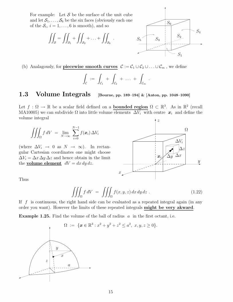
For example: Let S be the surface of the unit cubeand let S1, . . . ,S6 be the six faces (obviously each oneof the Si, i = 1, . . . , 6 is smooth), and so

∫∫

S

=

∫∫

S1

+

∫∫

S2

+ . . . +

∫∫

S6

.

PSfrag replacements

S1

S2S3

S4

S5

S6

(b) Analagously, for piecewise smooth curves C := C1 ∪ C2 ∪ . . . ∪ Cm , we define

∫

C

:=

∫

C1

+

∫

C2

+ . . . +

∫

Cm

.

1.3 Volume Integrals [Bourne, pp. 189–194] & [Anton, pp. 1048–1090]

Let f : Ω → R be a scalar field defined on a bounded region Ω ⊂ R3. As in R

2 (recallMA10005) we can subdivide Ω into little volume elements ∆Vi with centre xi and define thevolume integral

∫∫∫

Ω

f dV = limN→∞

N−1∑

i=0

f(xi) ∆Vi

(where ∆Vi → 0 as N → ∞). In rectan-gular Cartesian coordinates one might choose∆Vi = ∆x ∆y ∆z and hence obtain in the limitthe volume element dV = dx dy dz.

PSfrag replacements

x

y

z

∆x∆y

∆z

∆Vi

xi

Ω

Thus

∫∫∫

Ω

f dV =

∫∫∫

Ω

f(x, y, z) dx dy dz . (1.22)

If f is continuous, the right hand side can be evaluated as a repeated integral again (in anyorder you want). However the limits of these repeated integrals might be very akward.

Example 1.25. Find the volume of the ball of radius a in the first octant, i.e.

Ω := x ∈ R3 : x2 + y2 + z2 ≤ a2, x, y, z ≥ 0.

PSfrag replacements x

y

za

15

Things may become even nastier if we want to integrate over the entire ball.

1.3.1 Change of Variables – Reparametrisation

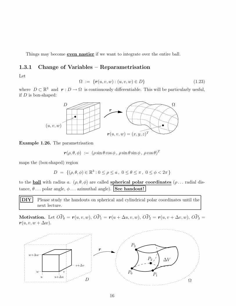
LetΩ := r(u, v, w) : (u, v, w) ∈ D (1.23)

where D ⊂ R3 and r : D → Ω is continuously differentiable. This will be particularly uesful,

if D is box-shaped:

PSfrag replacements ΩDr

(u, v, w)

r(u, v, w) = (x, y, z)T

Example 1.26. The parametrisation

r(ρ, θ, φ) := (ρ sin θ cos φ , ρ sin θ sin φ , ρ cos θ)T

maps the (box-shaped) region

D = (ρ, θ, φ) ∈ R3 : 0 ≤ ρ ≤ a , 0 ≤ θ ≤ π , 0 ≤ φ < 2π

to the ball with radius a. (ρ, θ, φ) are called spherical polar coordinates (ρ . . . radial dis-

tance, θ . . . polar angle, φ . . . azimuthal angle). See handout!

DIY Please study the handouts on spherical and cylindrical polar coordinates until thenext lecture.

Motivation. Let ~OP0 = r(u, v, w), ~OP1 = r(u + ∆u, v, w), ~OP2 = r(u, v + ∆v, w), ~OP3 =r(u, v, w + ∆w).

PSfrag replacements

ΩD

r

∆V

P0 P1

P2

P3

u

vw

u+∆u

v+∆v

w+∆w

16

For ∆u, ∆v, ∆w sufficiently small ∆V will be approximately a parallelepiped.

Recall (MA10006): PSfrag replacements

a

bcn

V

A

and in the limit as ∆u, ∆v, ∆w → 0

dV =

∣

∣

∣

∣

(

∂r

∂u∧ ∂r

∂v

)

· ∂r

∂w

∣

∣

∣

∣

du dv dw (1.24)

the so-called volume element.

Definition 1.27. The volume integral of a scalar field f : Ω → R over the region Ω ⊂ R3

in (1.23) is defined as∫∫∫

Ω

f dV =

∫∫∫

D

f(r(u, v, w))

∣

∣

∣

∣

(

∂r

∂u∧ ∂r

∂v

)

· ∂r

∂w

∣

∣

∣

∣

du dv dw . (1.25)

17

Note. Definition 1.27 is no contradiction to the change of variables formula which youhave learnt in MA10005, since

∣

∣

∣

∣

(

∂r

∂u∧ ∂r

∂v

)

· ∂r

∂w

∣

∣

∣

∣

= det

∂r1

∂u

∂r2

∂u

∂r3

∂u∂r1

∂v

∂r2

∂v

∂r3

∂v∂r1

∂w

∂r2

∂w

∂r3

∂w

=:∂(x, y, z)

∂(u, v, w)(1.26)

i.e. the Jacobian determinant.

[ Proof. (recall MA10006)

Remark 1.28.

(a) u, v, w can be regarded as curvilinear coordinates on Ω. (See the figure at the begin-ning of Section 1.3.1.)

(b) The integral (1.22) in Cartesian coordinates is just a special case with r(x, y, z) =

(x, y, z)T , and so∣

∣

∣

(

∂r∂x

∧ ∂r∂y

)

· ∂r∂z

∣

∣

∣= 1.

(c) The volume of Ω in (1.23) is a special volume integral, i.e. VΩ =∫∫∫

ΩdV .

Example 1.29. Redo Example 1.25 using spherical polar coordinates.

Step 1. Parametrise (see handout):

Step 2. Calculate the volume element dV =∣

∣

(

∂r∂u

∧ ∂r∂v

)

· ∂r∂w

∣

∣ du dv dw :

18

Step 3. Evaluate Formula (1.25) for the volume integral:

19