Embed Size (px)
Citation preview

1
Radar Data Assimilation &
Forecasts of Evolving Nonlinear Wave Fields
Sina H. AraghPh.D. Research Prospectus
Department of Naval Architecture and Marine Engineering
University of Michigan
Friday, May 4, 2007

2
Overview
• Introduction Research Problem Motivation
• Literature Review Marine Radars Wave Model Data Assimilation
• Methodology Forward Wave Model Assimilation Scheme Adjoint Wave Model Minimization Scheme
• Summary

3
Research Problem
Numerical Wave ModelRadar Image
Data Assimilation
Improved Estimate of the Wave Field
Short term Forecast

4
Research Objectives
• Develop an efficient numerical wave model that:
1) Captures basic nonlinear interactions
2) Predict nonlinear evolution of
multi-directional sea states
• Determine an optimal strategy to assimilate real-time radar observations into short-term forecast wave model to:
1) Provide improved estimates of the wave field
2) Forecast the short-term evolution of sea state

5
Motivation-Aircraft Landing-Optimal Path of Automated Vessels-Launch/Recovery
Eisenhower Carrier Aircraft Landing
Laun
ch/R
ecov
ery

6
Motivation(Rogue Waves)
t(sec)x(m)
Time history @ mid-length
Rock n’ Role
Rogue Waves

7
Literature Review(Marine Radars)
Marine radars can be used as a remote sensing tool to survey ocean wave fields
The wave measurement due to interaction of electromagnetic waves with sea surface ripples
This interaction produces a backscatter phenomenon showing a wave pattern in the radar screen (“sea clutter”)
“Sea clutter” is the required signal to get appropriate sea state characterization

8
Radar Imaging Mechanisms
Literature Review
(Marine Radars)

9
Literature Review(Marine Radars)
• Ijima et al.(1965) & F. Wright(1965)Among the first to use marine radars for imaging ocean waves
• Oudshoorn(1960), Willis & Beaumont(1971), Evmenov et al.(1973)Mean wave direction, Wave length, and Period
• Hoogeboom & Rosenthal(1982), Ziemer et al.(1983)Digitized radar images / 2D F.T. / Compared with Buoy Data
Major Problem with 2D wave number spectra: 180 degree directional ambiguity
• Atanassov et al.(1985)Removed the ambiguity in direction
• Young and Rosenthal1985)Used 3D F.T. / 3D energy density spectrum (wave number-frequency space)
Found the Mean current through least squares
High signal-to-noise ratio
• Estimates of significant wave height/instantaneous wave fields, requires knowledge of “Transfer Function”

10
Literature Review (Marine Radars)
• Alpers & Hasselmann(1978)Included shadowing/tilting, used signal processing in frequency domain to improve SNR, simpler hydrodynamic interaction / action balance • Ziemer & Rosenthal(1987)MTF in Fourier space, based on tilting/shadowing/hydrodynamicNonlinear influence mainly due to shadowing• Nieto Borge(1999)Directional spectrum/Significant wave height (based on its relation to SNR)Found correlation factor = 0.89 btw buoy and “WaMoS”• Nieto et al.(2004)Empirical scheme for inversion based on shadowing onlyApproach: 1) 3D Fourier decomposition amplitude & phase spectra 2) high-pass filtering remove long range effects 3) band-pass filtering extract wave-related components 4) I.F.T and re-scaling Wave amplitude
• Rosenthal & Dankert(2004)Based on determination of surface tilt angle in antenna look direction at each pixel of radar image
11
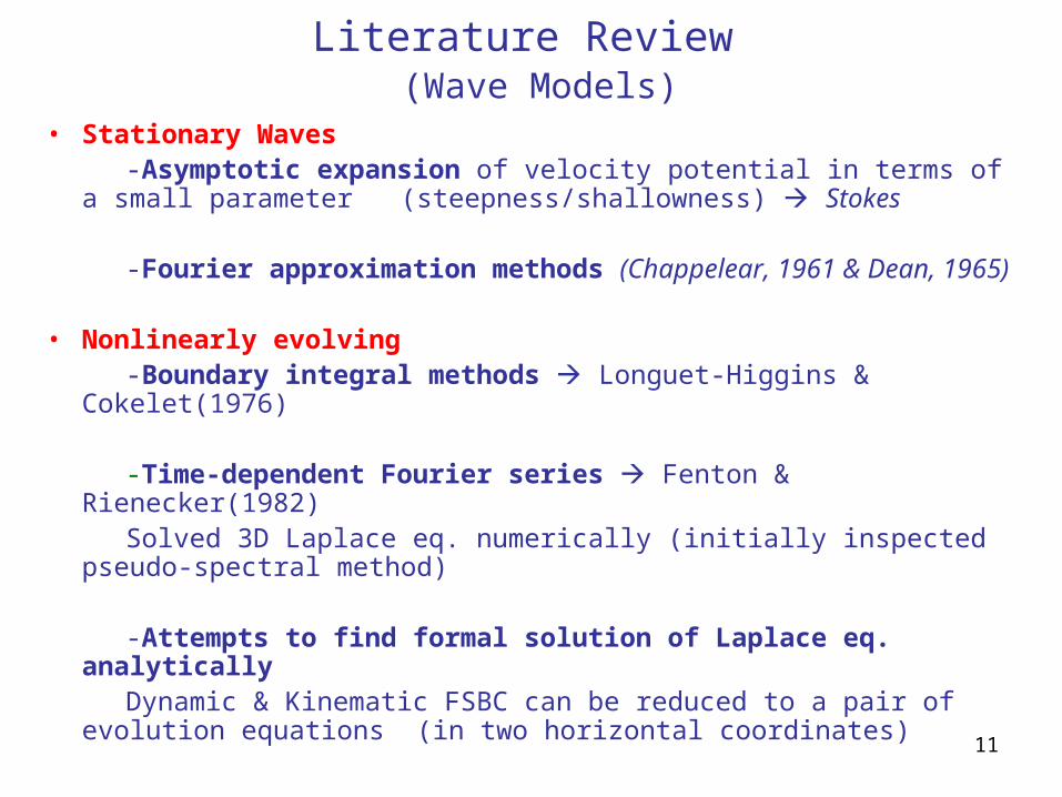
Literature Review (Wave Models)
• Stationary Waves -Asymptotic expansion of velocity potential in terms of a small
parameter (steepness/shallowness) Stokes
-Fourier approximation methods (Chappelear, 1961 & Dean, 1965)
• Nonlinearly evolving -Boundary integral methods Longuet-Higgins & Cokelet(1976)
-Time-dependent Fourier series Fenton & Rienecker(1982) Solved 3D Laplace eq. numerically (initially inspected pseudo-spectral
method)
-Attempts to find formal solution of Laplace eq. analytically Dynamic & Kinematic FSBC can be reduced to a pair of evolution
equations (in two horizontal coordinates)

12
Literature Review(Wave Models)
Two evolution equations
Need to close the system
Three surface variables
West et al.(1987) Asymptotic expansions (successive inversion of asymptotic sequences)
Matsuno(1992) 2nd order approximation
Craig & Sulem(1993) Expanding Dirichlet-Neumann operator / for constant depth, later extended by (Guyenne & Nickols, 2005) to variable depth
Choi(1995) 3rd order approximation (Similar to West et al.)
Clamond & Grue(2001) Formulated higher order effect by an integral representation
Similar approaches for long waves by Wu(1998, 2001), Madsen, Bingham, and Liu(2002), and Madsen, Bingham, Schaffer(2003)

13
Literature Review(Data Assimilation)
“Data Assimilation” is defined as finding the optimal initial/boundary conditions that minimize the difference between the measurements and model predictions over a time interval.
Data Assimilation
SequentialVariational
• Sequential Schemes:
Kalman Filter(Gelb, 1974)
+Optimal for linear problems
Direct Insertion(Daley, 1991)
+Spurious Oscillations

14
Literature Review(Data Assimilation)
Sequential schemes
Nudging (Kistler, 1974, Hoke & Anthes, 1976) choose nudging time scale is important
Successive Corrections (Bergthorsson & Doos, 1955) weighting functions/radius of influence
Variational Methods
Cost function is defined as the difference between model predictions and observations
Goal minimize the cost function over assimilation period
Gradient of the cost function with respect to initial conditions is needed
Good for large-scale
15
Literature Review(Data Assimilation)
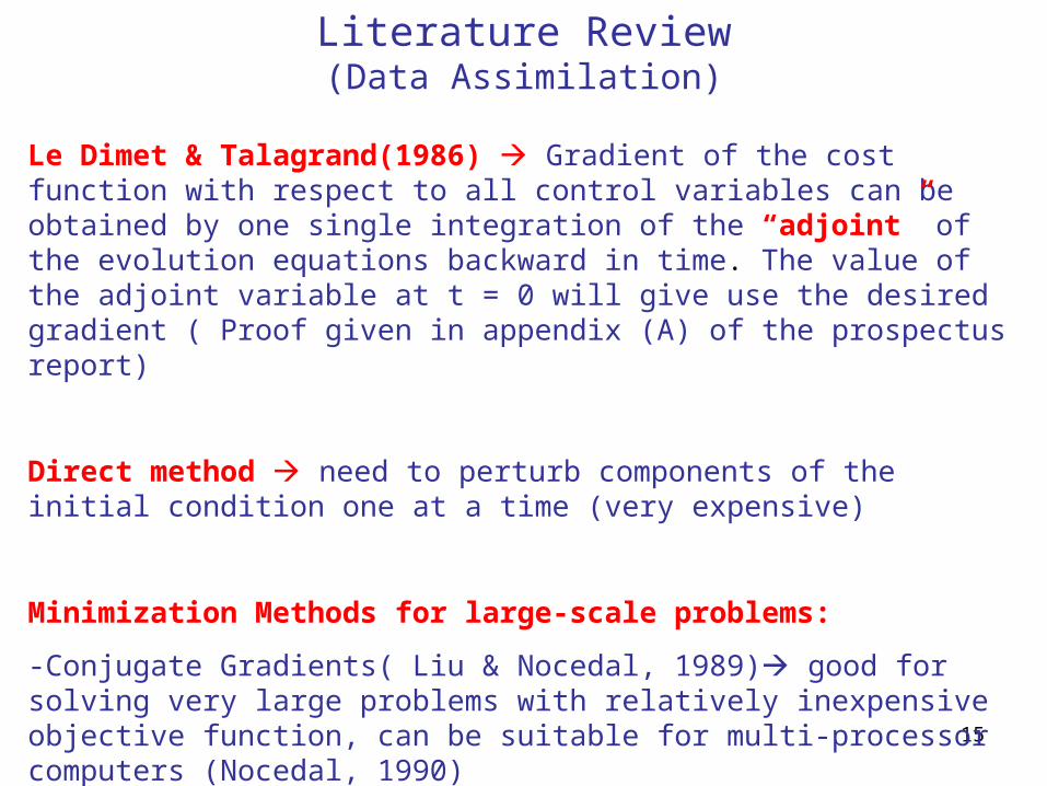
Le Dimet & Talagrand(1986) Gradient of the cost function with respect to all control variables can be obtained by one single integration of the “adjoint” of the evolution equations backward in time. The value of the adjoint variable at t = 0 will give use the desired gradient ( Proof given in appendix (A) of the prospectus report)
Direct method need to perturb components of the initial condition one at a time (very expensive)
Minimization Methods for large-scale problems:
-Conjugate Gradients( Liu & Nocedal, 1989) good for solving very large problems with relatively inexpensive objective function, can be suitable for multi-processor computers (Nocedal, 1990)
Search direction an estimate of the relative change in each component of the control vector to produce max. reduction in the cost function

16
Path to Methodology
Challenges:
• Large set of observational data (High resolution)• Complexity of modulation mechanisms • Nonlinearity of the sea state• Large sets of control parameters to optimize• Cost function does not directly depend on the
initial/boundary conditions• Need fast wave model / Efficient optimization scheme

17
Methodology(Forward Wave Model)
Zakharov(1968)(Hamiltonian Formulation)
P.E.K.E.
Canonical Pair
Free surface evolution equations
=

18
Forward Wave ModelExpanding about z = 0
Where :
Closure:
Solving the linear boundary value problem
(Matsuno, 1992)
Fourier Space
Physical Space

19
Forward Wave Model
Inversion
First order evolution eq.
Third order evolution eq.

20
Numerical Solution of Forward Wave ModelPseudo-spectral method used to solve the evolution equations
Linear operators Fourier Space
NL operators Physical space
RK-4 used to integrate in time

21
Validating wave model with experimental data(NRC)
• Two wave makers at both sides / totally 168 segments
• 25m long boom with 20 probes
• 5 fixed probes
• Generating various multi-directional sea states
• Nonlinear interactions between crossing waves

22
Validating numerical wave model with experimental data(NRC)

23
Assimilation Scheme
•Determine optimal set of initial conditions, boundary conditions and model parameters that minimize differences between model predictions and radar observations over assimilation interval
Cost Function:
Objective:
•Use optimal set of initial conditions, boundary conditions and model parameters to forecast wave field evolution
•After preliminary tests of different schemes, chose adjoint-based method
•Conjugate gradients used for minimization
•Gradient of the cost function w.r.t. initial condition obtained from adjoint technique

24
Adjoint Data Assimilation
InitializeModel
Prediction - Observation
Prediction - Observation
Prediction - Observation
Forward Model
Adjoint Model
Prediction - Observation
Prediction - Observation
Prediction - Observation
InitializewithError
Grad ofCost
Function
Conjg.Gradient
Min.
Short-term forecast
Assimilation Interval
(0 T)
t = Tt = 0
Adjoint Data Assimilation
25
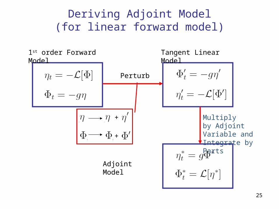
Deriving Adjoint Model(for linear forward model)
Adjoint Model
1st order Forward Model
Perturb
Tangent Linear Model
Multiplyby Adjoint Variable andIntegrate by Parts
+
+

26
Third-Order Equations Forward Model
Tangent Linear Model

27
Third-Order Equations
Adjoint Model

28
Evaluation of Gradient Computations
• Domain length = 3066m; Grid spacing = 6m, Time Step = 0.25s
• Added 10% uncorrelated noise to 16 model predictions at intervals of 2.5s
• Selected JONSWAP sea state with Hs = 2m, Tp = 10s
• Compared adjoint prediction of gradient of cost function with direct sensitivity method

29
Proposed Approach(Adjoint vs. Direct method – 1st order)
400 500 600 700 800 900 1000-1.5
-1
-0.5
0
0.5
1
1.5
spatial domain
Gra
die
nt
of
the
co
st
fun
cti
on
w.r
.t. i
nit
ial c
on
dit
ion
Adjoint method
Direct method
Numerical tests with JONSWAP sea state

30
Proposed Approach(Adjoint vs. Direct method – 3rd order)
Numerical tests with JONSWAP sea state

31
Ability to Reproduce Initial Condition with Noisy Model Prediction used as “Observation”
2400 2450 2500 2550 2600 2650-2
-1.5
-1
-0.5
0
0.5
1
1.5
2
spatial domain(x)
Su
rfa
ce
ele
va
tio
n @
t =
0
noisy initial cond.
true state
assimilated

32
Ability to Reproduce Initial Condition with Noisy Model Prediction used as “Observation”
0 0.02 0.04 0.06 0.08 0.1 0.12 0.14 0.16 0.180
1
2
3
4
5
k
S(k
) @
t =
0
noisy initial condition
true state
assimilated

33
Ability to Reproduce Initial Condition with Noisy Model Prediction used as “Observation”

34
Time history of the surface elevation at x = L/4, forecasted from the produced optimal initial condition.
Noisy model predictions were used as “observation”
0 10 20 30 40 50 60 70 80-1
-0.8
-0.6
-0.4
-0.2
0
0.2
0.4
0.6
0.8
1
time(s)
Su
rfa
ce
ele
va
tio
n(m
)time history @ x = 0.25L
with noisy I.C.
true stateassimilated

350 10 20 30 40 50 60 70 80
-1.5
-1
-0.5
0
0.5
1
1.5
time(s)
Su
rfa
ce
ele
va
tio
n(m
)time history @ x = 0.5L
with noisy I.C.
true state
assimilated
history of the surface elevation at x = L/2, forecasted from the produced optimal initial condition. Noisy model
predictions were used as “observation”.
36
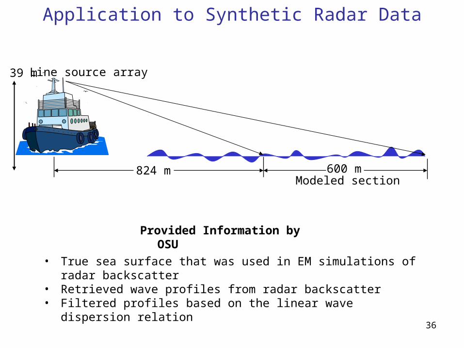
Application to Synthetic Radar Data
600 m824 m
39 m
Modeled section
Line source array
• True sea surface that was used in EM simulations of radar backscatter• Retrieved wave profiles from radar backscatter• Filtered profiles based on the linear wave dispersion relation
Provided Information by OSU

37
Synthetic Radar Data (OSU)
From: Johnson et al. (2006)

38
Application to Synthetic Radar Data
0 100 200 300 400 500 600-4
-3
-2
-1
0
1
2
3
4
5
x-domain
surf
ace
elev
atio
n(m
)
Surface elevation @ t = 0
retrieved from radartrue stateassimilated
Ability to Reproduce Initial Condition with True Sea State used as “Observation”

39
Ability to Reproduce Initial Condition with True Sea State used as “Observation”
0 20 40 60 80 100 120 140 160 18010
0
101
102
103
iteration
Co
st F
un
ctio
n
Application to Synthetic Radar Data
40
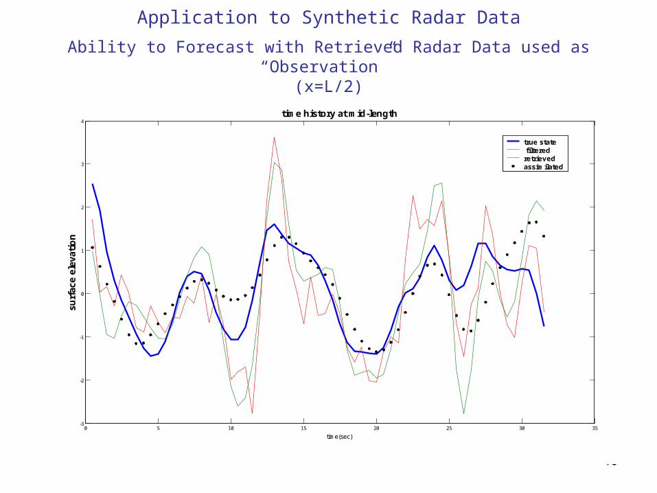
Application to Synthetic Radar Data
0 5 10 15 20 25 30 35-3
-2
-1
0
1
2
3
4
time(sec)
surf
ace
elev
atio
n
time history at mid-length
true state filteredretrievedassimilated
Ability to Forecast with Retrieved Radar Data used as “Observation” (x=L/2)

41
Application to Synthetic Radar DataAbility to Forecast with Filtered Radar Data used as “Observation”
(x=L/2)

42
Field Data (Alaska, Sept. 2006)
•Evaluate the performance and limitations of both Doppler (coherent) and non-coherent X and S-band radars for the real-time measurements of ocean wave fields
•Validate of nonlinear wave evolution model
•Validate data assimilation and forecast scheme

43
Future Plans
Test different optimization schemes with synthetic data
Extend assimilation scheme to boundary conditions
Improve efficiency of the assimilation scheme by defining
control variables in Fourier space instead of physical space
Develop 2-D model and validate model with lab data
Develop 2-D assimilation scheme and compare with field data