Embed Size (px)
Citation preview

1
Submitted to: Journal of Geophysical Research-Atmospheres
(Manuscript Number: 2004JD005318)
Submitted on August 5th
, 2004
Revised on October 8th
, 2004
Corresponding author:
Fatima KARBOU
10-12, Avenue de l’Europe
78140, Vélizy, France
Email: [email protected]
Tel. + 33 1 39 25 39 28
Fax: +33 1 39 25 47 78
Potential of AMSU-A and -B measurements for atmospheric
temperature and humidity profiling over land
Fatima KARBOU
CNRS / IPSL / CETP, France
Filipe AIRES
CNRS / IPSL / LMD, France
Catherine PRIGENT
CNRS / Observatoire de Paris / LERMA, France
Laurence EYMARD
CNRS / IPSL / LODYC, France

2
Abstract— A neural network retrieval method has been applied to investigate AMSU-A/-B
atmospheric temperature and humidity profiling capabilities over land. The retrieval method
benefits from a reliable estimate of the land emissivity and skin temperature as well as first guess
information regarding the temperature-humidity profiles. It has been applied on a large geographic
area (60°W-60°E; 60°S-60°N) and atmospheric situations (winter and summer). The retrieved RMS
errors are within 2 K and 9% in temperature and relative humidity respectively. Regardless
scanning conditions, vegetation types and atmospheric situations, the algorithm retrieval results are
satisfactory for both temperature and relative humidity. The retrieval approach has been evaluated
by comparison with available in situ measurements.
Index Terms—AMSU, microwave surface emissivity, atmospheric temperature and humidity
profiles.

3
1 INTRODUCTION
The Advanced Microwave Sounding Unit (AMSU) A and B on board the latest generation of the
National Oceanic and Atmospheric Administration (NOAA) polar orbiting satellites measure the outgoing
radiances from the atmosphere and the Earth surface. With channels in the oxygen absorption band,
AMSU-A is designed to retrieve the atmospheric temperature from about 3 hPa (~45 km) down to the
Earth's surface. AMSU-B module makes measurements in the vicinity of the strong water vapor absorption
line at 183 GHz and is used for atmospheric water vapor sounding. Therefore, the use of AMSU
measurements in operational Numerical Weather Prediction (NWP) models can potentially provide
accurate monitoring of both air temperature and moisture profiles with good temporal and spatial
sampling. Compared to infrared sounding measurements, AMSU observations are less sensitive to high
thin and non precipitating clouds.
Several retrieval techniques have been developed for temperature and/or humidity sounding with
AMSU-A/-B and other microwave radiometers measurements. Rosenkranz [2001] used surface and
atmosphere modeling to retrieve temperature-moisture profiles from AMSU-A/B data. Wagner et al.
[1990] retrieved humidity profiles using passive microwave measurements. A neural network technique
has been used by Shi [2001] to estimate air temperature profiles from AMSU-A; a similar technique has
been utilized by Franquet [2003] for 3-D restitution of water vapor using microwave satellite instruments.
Over ocean, the AMSU measurements are now routinely assimilated in NWP systems and they provide
unique atmospheric profiling capabilities. Over land however, the AMSU measurements are not fully
exploited. At best, only the channels that are not contaminated by surface contributions are assimilated,
thus limiting the profiling potential to the higher atmospheric layers. Kelly and Bauer [2000] describe the
current use of 10 AMSU channels measurement in the European Centre for Medium-Range Weather
Forecasts (ECMWF) assimilation system. Recent efforts to assimilate AMSU radiances over ocean/land
are performed at many NWP centers [TOVS study conference, 2003]. Contrarily to the ocean emissivity,
the land surface emissivity is high, often close to unity, leading to difficulties in discriminating between
surface and atmosphere contributions. In addition, the land emissivity exhibits complex temporal and
spatial variations, depending on surface types, roughness, and moisture content, among other parameters.
As a consequence an accurate estimate of the microwave land emissivity is a prerequisite for a full
exploitation of satellite sounding measurements over land. Recent works focused on the development and
analysis of emissivity estimates at AMSU frequencies and observation conditions [Karbou et al., 2004],

4
following the method developed for the Special Sensor Microwave/ Imager [Prigent et al., 1997; 1998]. It
is thus now possible to develop retrieval techniques to fully benefit from microwave sounder
measurements over land, as it has already been done for microwave imagers [Prigent and Rossow, 1999;
Aires et al., 2001].
The objective of this paper is to study the feasibility of use of all AMSU-A and –B channels over land
for retrieving atmospheric temperature and moisture profiles down to the surface; then to evaluate the
performances of the retrieval method by quantifying the information content of the AMSU-A and -B
observations for such retrievals over land. The final aim of this study is to investigate and prepare the
assimilation (variational method) of all AMSU channels measurements over land in NWP models. The
information content analysis is based on neural network (NN) statistical approach, with use of a first guess
profile and auxiliary information (surface temperature and emissivity). Compared to more traditional
information content techniques [Rodgers, 1990], using a NN has the advantage of requiring none of
theoretical assumptions such as linearity or the Gaussian character of the variables. Our approach consists
in designing a NN retrieval scheme procedure, to apply it to a large set of realistic atmospheric situations,
and to analyze the impact of the satellite observations on the retrieved products. Two contrasted months of
AMSU data are analyzed over a large part of the globe centered on Africa. In this preliminary study, only
cloud free data have been selected to conduct the atmospheric retrievals. Given the scarcity of the
radiosonde measurements over large parts of Africa, it is of primary importance to get reliable satellite
estimates of the temperature and humidity profiles in this region.
The AMSU observations and the emissivity dataset are described in section 2. The retrieval approach is
presented in section 3 and its results are analyzed with respect to the AMSU zenith angle, season, and the
vegetation type. Additional analysis regarding the ECMWF first guess information is provided in section 4
as well as an evaluation of the retrieval method by comparison with radiosonde measurements. Section 5
concludes this study.
2 SATELLITE OBSERVATIONS AND EMISSVITY DATASETS
2.1 AMSU-A AND -B MEASUREMENTS
The AMSU sounding unit operates on board the NOAA satellites since 1998. AMSU-A has 12 channels
located close to the oxygen absorption lines below 60 GHz and four window channels at 23.8, 31.4, 50.3,
and 89 GHz. AMSU-B has two window channels at 89 and 150 GHz and three channels centered on the
183.31 GHz water vapor line. The two instruments have instantaneous fields of view of 3.3° and 1.1° and

5
sample 30 and 90 Earth views respectively. Therefore, the AMSU observation scan angle varies from -48°
to +48° with the corresponding local zenith angle reaching 58°. Channel characteristics for both AMSU-A
and -B radiometers are given in Table 1 and a detailed description of the AMSU sounders is reported in
Goodrum et al. [2000].
Level 1b AMSU data have been obtained from the Satellite Active Archive (SAA) and processed using
the Advanced ATOVS Processing Package (AAPP) created and distributed by EUMETSAT and co-
operations. The AMSU radiances are corrected from the AMSU antenna effect using coefficients given by
Mo [1999] and Hewison et al. [1996]. The analysis in this study is made at AMSU-A spatial resolution.
Data have been selected to cover a large geographic area including mainly Africa but also Eastern South
America, Southern Europe, and the Middle East (from 60°W to 60°E in longitude and from 60°S to 60°N
in latitude). The study is performed for January and August 2000. At that time, NOAA 15 is in sun-
synchronous polar orbit and crosses the equator at local solar times of approximately 7:30 a.m. and 19:30
p.m.
In the present work, the AMSU information content analysis is conducted over land and under cloud
free situations. Once our experience results are thoroughly validated, the analysis will be extended to
cloudy situations. Clouds have a complex and highly variable impact on the observed microwave
radiances, depending on both the cloud property and the observation frequency. Cloud screening is
conducted using the International Satellite Cloud Climatology Project (ISCCP) datasets. Cloud parameters
and skin temperatures are extracted from the ISCCP pixel level data (the DX dataset) for January and
August 2000. These products are available at 30 km ground resolution every 3 hours. Within ISCCP,
information about clouds is obtained from visible and infrared measurements from polar and geostationary
satellites, using radiative analysis [Rossow and Schiffer, 1991].
Figure 1 shows the weighting function distributions for all AMSU channels calculated for a US standard
tropical atmosphere at nadir using a microwave radiative transfer model [Pardo et al., 2001]. The
weighting functions indicate the relative contribution of each atmospheric layer to the measured radiance.
For a given atmosphere and frequency, the peak altitude in the weighting function increases with
increasing zenith angle. This is due to increasing optical path length between the satellite and the Earth
when the instruments scan from nadir to higher angles. In window channels the weighting function peaks
have their maximum closer to the surface. Most of the radiation measured by these window channels
comes from the surface and the boundary layer and these channels can be used to derive total precipitable
water, precipitation rate, or cloud liquid water over ocean [Grody et al., 2001; Zhao and Weng, 2002,
Weng et al. 2003]. For all the channels that have some contribution coming from the surface, it is
important to accurately estimate the surface emission in order to correctly separate its effect from the
atmospheric one.

6
AMSU observes the Earth with a large range of angles leading to difficulties when developing retrieval
algorithms: the angular dependence has to be taken into account in the inversion algorithm. Alternative
techniques have been developed to convert the observed radiance at a given angle to the radiance that
would be measured at nadir. Goldberg et al. [2001] for instance describe the limb adjustment of AMSU-A
observations to nadir. In the present study, no limb correction method is applied. All AMSU-A scan
positions are considered and the retrieval accuracy will be evaluated for all angles. Figure 2 shows the
mean Brightness Temperatures (Tbs) against the local zenith angle observed for cloud-free situations in
January and August 2000. The observations have been sorted by vegetation types using the Biosphere-
Atmosphere Transfer Scheme (BATS) vegetation land cover dataset (available at 30×30 km grid
resolution) [Dickinson et al., 1986]. The angular variations of the Tbs are driven by two phenomena,
depending on the channel opacity: for window channels the angular dependence of the emissivity prevails
whereas for sounding channels the opacity increase with angle is the dominant effect. Surface and near-
surface channels (23.8, 31.4, 50.3, 89.0, and 150 GHz) Tb curves show similar trends than those observed
while analyzing the angular emissivity variation [Karbou et al., 2004]. Figure 3 shows the mean monthly
emissivities at 31.4 GHz over desert, calculated for 6 months of data, and sorted by beam observation
angle; the emissivity curve show similar trend than the mean Tb curve at 31.4 GHz over desert (Figure 2).
Most of the angular variations in surface and near-surface channels are related to the surface emissivity
angular dependence. Mo [2002] made similar observations when comparing mean Tbs and emissivities
from AMSU-A channels over the Libyan Desert. As a consequence, an accurate estimate of the emissivity
is required for the full incidence angle ranges to properly account for the surface contribution to the
measured radiance at each scan angle.
For this purpose, the microwave land surface emissivities at AMSU frequencies have been studied
[Karbou et al., 2004] and this work is briefly described in the next section.
2.2 AMSU LAND EMISSIVITY CALCULATIONS
The AMSU land surface emissivities have been calculated under the assumption of a flat and specular
surface, using data from year 2000, for 30 observation zenith angle ranges (from -58° to +58°) and for the
23.8, 31.4, 50.3, 89, and 150 GHz channels after separating cloud and atmospheric contributions [Karbou
et al., 2004]. For the emissivity calculations only cloud free data have been considered. Collocated
visible/infrared satellite measurements from ISCCP data have been used to screen cloud and rain effects
and to provide an accurate estimate of the skin temperature. The nearby temperature-humidity profiles
from the ECMWF [Simmons and Gibson, 2000] have been used as input into a state-of-the-art microwave

7
radiative transfer model [Pardo et al., 2001] in order to estimate the atmospheric contribution to the
measured radiances.
The obtained monthly-mean emissivity maps show the expected spatial structures, related to changes in
surface types. Lakes and rivers as well as the coastlines are associated with low emissivities at all
frequencies but also with high emissivity variability. For the entire datasets, the day-to-day emissivity
standard deviations are generally less than 2% in AMSU surface channels and tend to increase with
frequency and zenith angles. English [1999] showed that the use of land emissivity with accuracy better
than 2% would help humidity profile retrievals over land. For all frequencies, the emissivities depend on
the incidence angle, especially for bare soil areas. Figure 3 illustrates this angular variation at 31.4 GHz
for desert surfaces for 6 months of data. This Figure also shows an asymmetry along the AMSU scan,
relatively to nadir, variable with frequency and surface emissivity. For all vegetation classes, the AMSU
scan asymmetry is found to be higher at 31.4 GHz than at the other frequencies. The maximum scan
asymmetry (difference between the monthly mean emissivities at scan position 1 and 30) for this channel
reaches up to 3% over desert areas. The 23 GHz channel is also affected by the scan asymmetry but the
magnitude of this effect is smaller (2.4 % over desert surfaces). Measurements at 89 GHz appear to be less
sensitive to the scan asymmetry than those at 50.3 GHz. Weng et al. [2003] also noticed an asymmetry in
AMSU surface channels by using AMSU ocean observations and simulations. The AMSU scan asymmetry
is likely related to an instrument calibration problem. For effective retrievals of atmospheric variables over
ocean and land, the instruments have to be accurately calibrated for all conditions (frequencies and
scanning positions). This asymmetry is being investigated in order to suggest adequate corrections. The
likely instrumental problem is accounted for by using mean emissivities sorted by scan position.
Therefore, in the present study, the observations are systematically sorted by scan position angle. Pre-
calculated AMSU mean monthly emissivity maps for January and August 2000, with a ground resolution
of 30x30 km, and at 23, 31, 50, 89 and 150 GHz are used to characterize the land contribution to the
measured radiances. The emissivities in the sounding channels have not been calculated because the
surface contribution at these frequencies is not strong enough to derive reliable estimates. Given the
smooth and limited frequency dependence of the land surface emissivities in this wavelength range
[Prigent et al., 2000; Karbou et al., 2004], the emissivities in the window channels can be extrapolated
from their estimates in the nearest sounding channels. For example, mean emissivities at 50 GHz have
been used for channels in the vicinity of the 50-60 GHz channels band. By the same token, emissivities
calculated at 150 GHz have been used for the 183.31 GHz channels.

8
3 AN INFORMATION CONTENT ANALYSIS
3.1 THE NEURAL NETWORK APPROACH
The first stage in developing a Neural Network (NN) retrieval scheme is to obtain a dataset of samples
describing the relationships between the inputs (i.e., satellite observations and a priori information) and
the outputs (i.e., variables to retrieve). For this purpose, AMSU measurements and collocated ECMWF re-
analyses [Simmons and Gibson, 2000] are selected. An alternative would be to simulate AMSU
observations with a radiative transfer model using ECMWF atmospheric profiles but in this case the
instrument noise would need to be specified, and this information is not directly available in this context.
For each AMSU measurement, the closest (in space and time) atmospheric situation from ECMWF to the
actual AMSU observation is defined as the target that the NN has to retrieve. Consequently, the procedure
includes several sources of observation errors: the instrument noise, differences in space/time collocation,
differences in spatial resolution, as well as the error of the ECMWF re-analysis itself related to the NWP
model errors.
The NN algorithm is developed to retrieve simultaneously the atmospheric temperature and humidity
profiles over land using AMSU-A and -B observations at 21 fixed pressure levels from 1000 to 1hPa. In
addition to satellite measurements, the NN retrieval scheme benefits from other sources of information: a
priori and first guess information can be used to better constrain the inversion problem and to limit non-
uniqueness and/or instabilities of the solution. This approach was developed by Aires et al. [2001] to
retrieve simultaneously water vapor, cloud liquid water path, surface temperature, and microwave
emissivities over land using SSM/I instrument. In the present study, the three sources of information
available to perform the retrieval are:
- All AMSU-A and -B satellite observations (i.e., 19 NN inputs corresponding to each
instrument frequency);
- The ECMWF atmospheric temperature and moisture profiles on 21 levels taken 6 hours before
the ECMWF target profiles are used as First Guess (FG) information (i.e., 2×21 NN inputs);
- Spatially and temporally collocated ISCCP skin temperatures as well as the previously
calculated emissivities at 23.8, 31.4, 50.3, 89, and 150 GHz are used as a priori information (i.e., 6
NN inputs). The emissivities vary with the geographic location but also with scan position and
specified month (January or August). For each channel and each geographic location, the standard
deviation of the day-to-day variations within a month has been calculated. The obtained standard
deviations are then associated to the mean emissivities during the learning stage. The day-to-day
variability of the emissivity is found within 2% for all frequencies [Karbou et al., 2004].

9
In order to retrieve the temperature and humidity profiles (i.e., 2×21 NN outputs), a multi-layered
perceptron [Rumelhart et al., 1986] is constructed with 67 inputs, 50 neurons in the hidden layer, and 42
outputs. A schematic structure of the NN inversion scheme is provided in Figure 4.
The dataset was constructed using cloud-free AMSU Tbs from January and August 2000 in order to
include a wide range of atmospheric conditions. The selected geographic area (60°W-60°E and 60°S-
60°N) is large enough to insure variability in surface and atmospheric conditions (from arid to very moist
areas). For both August and January months, 1/3 of the data are assigned to the test database whereas 2/3
of the data are attributed to the learning database. The applied data repartition allows for a good
disjunction between the learning and the generalization datasets. It should be noted that we experimented
different database selections (like random daily drawings) and we obtained similar statistics. This confirms
the robustness of our estimate of the generalization error.
3.2 THE RETRIEVAL RESULTS
Figure 5 shows the RMS error profiles for temperature and humidity obtained at 21 pressure levels from
1000 to 1 hPa, regardless of scanning angle, season, and surface types. At each level, the FG RMS error
profile is calculated using the difference between the target and the FG ECMWF profiles. Similarly, the
NN RMS error profile is calculated using the difference between the target and the retrieved profiles. For
both temperature and humidity, the retrieved profile is closer to the target profile than the FG profile,
showing the benefit of AMSU radiances associated with a reliable characterization of the surface
contribution. The improvement in temperature is significant at low (< 700 hPa) and at high (> 100 hPa)
levels: the RMS improvement (difference between the FG and NN RMS errors) is about 1.4 K at 1000 hPa
and greater than 0.9 K at levels higher than 10 hPa pressure. At the lowest level, the RMS errors decrease
from 3.5 K to 2.1 K for temperature and from 14.5% to 9.1% in relative humidity. In order to examine the
spatial structure of the NN retrieval accuracy, FG and NN RMS error maps are plotted in Figure 6 for both
temperature and humidity at 1000 hPa level. Before inversion, the maps of the difference between the FG
and the target profile, for both water vapor and temperature, show a very strong longitudinal structure
related to the difference between the local time of the satellite overpass and the synoptic times. The FG
and target profiles being derived from the reanalysis, they are systematically obtained at the synoptic times
(0, 6, 12, or 18UTC), and the time difference between these two profiles is always of 6 h. However, this
time difference translates into very different temperature or relative humidity differences in the profiles,
depending on the local time of the day at the given location. The maps illustrate the NN retrieval
improvement with homogenous RMS error over the geographic area to be within 2 K in temperature and

10
9% in humidity, regardless of the location longitude. In particular, areas with higher FG RMS error in
temperature and humidity (i.e., Arabian Desert, South America) are significantly improved by the NN.
There is no significant dependency between the retrieval accuracy and the surface characteristics: The NN
retrievals are satisfactory regardless of the surface type.
The previous RMS error profiles have been produced with all data (January and August) and at all
AMSU-A scan positions. In the next section, retrieval results are examined more closely with respect to
the AMSU-A scan position, the vegetation cover, and the season.
3.3 SCAN ANGLE AND VEGETATION DEPENDENCIES
AMSU-A and -B instruments scan from -58° to 58° from nadir. The retrieved products are now
analyzed to check for scan dependency in the retrieved temperature and humidity profile accuracy. Figure
7 compares the RMS error profiles in temperature and relative humidity at nadir (7.a) and at 58° from
nadir (7.b). No significant difference is observed along the profiles between the two scanning cases for
both temperature and humidity retrievals. In particular, at surface level, where scan dependencies could
likely be the greatest, no significant effect can be noticed. Figure 7.c represents the NN RMS errors at
1000 hPa level as a function of the AMSU zenith angle for both temperature and relative humidity, and
shows that no significant dependency exists between the surface level RMS errors and the zenith angle for
both temperature and humidity. The NN improvement is within 2 K for temperature and 9% for humidity
for all scanning situations; in particular, no significant deterioration of the retrievals is observed for high
zenith angles. To confirm the retrieval scheme homogenous results with the scan angle, we conducted 6
retrieval experiments by training 6 independent NN for 6 limited ranges of zenith angle ([-58°, -46°], [-
42°, -26°], [-22°, nadir], [nadir, 22°], [26°, 42°], and [46°, 58°]). Individual results from these experiments
(not shown) do not show better retrieval accuracy than the unique NN.
Retrieved products are now analyzed by season and vegetation characteristics. Figure 8 presents the
RMS error profiles for temperature and humidity calculated for desert and dense vegetation areas
separately. January and August data have also been separated and all scanning conditions have been
considered. For a given vegetation type, Figure 8 shows homogenous retrieval results for both temperature
and humidity, for January and August. A slight improvement of the humidity RMS error at surface level
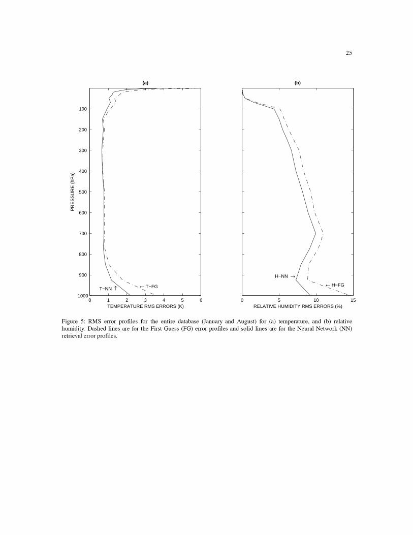
can be noticed in August for desert surfaces. Figure 9 completes this analysis by showing the RMS error
profiles of the retrieved parameters over desert and dense vegetation for both January and August, at nadir.
The NN retrieval performs well, regardless of season, scanning situations, and vegetation types. The
results show that when reliably characterizing the surface, we are able to correctly take into account the

11
surface variability with vegetation and scan observation angle and provides uniformly homogeneous
retrievals in very diverse situations, from dry desert regions to very moist equatorial areas. Significant
improvements are observed even in the lower atmospheric layers where surface contribution is important.
4 FURTHER ANALYSES
4.1 IMPACT OF THE FIRST GUESS TEMPERATURE AND HUMIDITY PROFILES
The previous analysis shows that by using temperature and relative humidity first guess profiles (i.e.,
ECMWF profiles 6 hour before the target ECMWF profile, called FG-06) along with accurate surface skin
temperature and emissivities, the surface effect on the AMSU measurements can be de-correlated from the
atmospheric one leading to atmospheric temperature/humidity retrievals over land. In this section we
examine the impact of the FG profiles choice on the NN retrievals. This is achieved by training NNs using
the same AMSU dataset but with two different FG scenarios: First, using ECMWF profiles 24 hours
before AMSU observations (called FG-24) and second, using the closest profile to the AMSU observation
time but with additive noise (called FG-NOISE). The noise characteristics are those of the ECMWF model
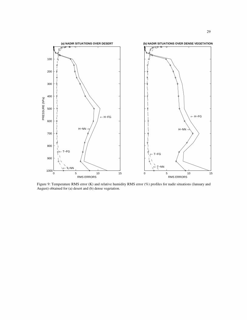
in 2000; these characteristics have been revised since. For specific humidity, the specification of the
standard deviations is established using several statistics including radiosonde observations and it depends
on the atmospheric situations [Rabier et al., 1998]. On the contrary, temperature standard deviations only
vary with latitude (i.e., different specifications for each 10° latitude range). The humidity noise is
calculated for each ECMWF profile taking into account the temperature, humidity, and pressure. The
temperature noise is calculated for ranges of latitudes over the studied area corresponding to (0-10°, 10°-
20°, 30°-40°, 40°-50°, and 50°-60°). Figure 10 shows a temperature-humidity profile from our database (a,
c) and the corresponding standard deviations for (b) temperature assuming different latitudes and (d)
specific humidity using Rabier et al. [1998] method.
Figure 11 (a, b, c) presents the temperature and relative humidity NN results for the different FG
scenarios: the RMS error profiles are plotted for the three FG configurations and for the corresponding NN
retrievals. For temperature, the FG-24H is of less quality than the FG-06H, except for lower levels where
the diurnal variability can be higher than the day-to-day changes. The FG-NOISE is always better than
FG-06H and FG-24H with standard deviation of errors already close to 0.5 K for each vertical layer: Not
surprisingly, in the FG-NOISE configuration, the use of AMSU satellite observations in the retrieval
scheme slightly improves the FG especially at high pressure levels; it can even degrade it in the lower
levels. For our retrieval method, The FG-06H and FG-24H configurations appear more adequate and the

12
retrieval at FG-06H has better statistics than the FG-24H. For relative humidity, all FG scenarios seem to
be adequate for our retrieval algorithm, and in all cases the FG is improved by the NN retrieval. Best
humidity retrievals are obtained using the FG-06H and FG-NOISE scenarios. From this set of experiments,
it can be seen that retrieval results are highly dependent on the FG profiles choice. In our information
content analysis, the temperature/humidity FG-06 scenario seems to be a good compromise: the obtained
statistics are satisfactory for both temperature and humidity retrievals (especially at atmospheric low
levels).
4.2 RETRIEVAL METHOD EVALUATION WITH RADISONDE DATA
Radiosonde observations provide independent and unique reference for temperature and humidity
profiles that can be used for satellite retrieval validation. However, their use for such evaluation has some
recognized limitations. For instance, they are unevenly distributed over the Earth with different
measurement accuracy. They are particularly scarce in Africa. Measurements are performed at fixed times
generally twice a day. They represent 1D information up to generally 100hPa whereas the satellite
measures a large atmospheric volume, from the bottom to the top of the atmosphere and with the
horizontal spatial extent related to the instrument field of view.
Records of radiosonde measurements are archived at many meteorological centers. For example, global
radiosonde datasets from 1998 to 2004 are produced jointly by the National Climatic Data Center (NCDC:
http://www.ncdc.noaa.gov) and the Forecast Systems Laboratory (FSL: http://www.fsl.noaa.gov).
Radiosonde stations located within the studied geographic area (60°W-60°E and 60°S-60°N) and
operational during January and August 2000 have been collocated in space and time with AMSU
observations. Table 2 lists the selected radiosonde stations with their locations. These stations produce
daily temperature and humidity profiles at 0 and at 12 UTC. During 2000, only the NOAA 15 satellite was
operational with equator crossing at 7:30 a.m. and 19:30 p.m. As a consequence, there is at least 3 hours
difference between the AMSU and selected radiosonde observation times.
Figure 12 shows the RMS error profiles obtained by comparing the FG and the NN retrieval with the
collocated radiosonde measurement. As expected, the FG errors as compared to radiosondes are rather
large, but we already commented in the beginning of this section on the limitations of radiosonde
comparisons, in particular considering the large space and time differences in the collocation process.
Since the FG RMS error profiles include large collocation errors, the detection of a relative improvement
is difficult. At surface level however, the RMS error is improved by about 2 K in temperature and 2.5% in
humidity. This confirms that, when associated to careful design of retrieval technique, AMSU-A and -B
observations can help retrieve low-level temperature and humidity profiles over land.

13
5 SUMMARY AND CONCLUSIONS
This paper studied the feasibility of AMSU temperature and humidity profile retrieval over land, down
to the surface. A neural network retrieval algorithm was developed, in which the AMSU satellite
observations were combined with a priori surface skin temperature and surface emissivity, and with first
guess information on the atmospheric profiles. The retrieval method has been applied over a large
geographic area including mainly Africa but also Eastern South America, Southern Europe, and the Middle
East (from 60°W to 60°E in longitudes and from 60°S to 60°N in latitudes). A very large number of
atmospheric situations have been considered for our experiment, from a winter and a summer month. The
NN retrievals over this large dataset is used as an information content analysis aiming at the evaluation of
the potential of AMSU observations in improving low-level temperature and humidity profiles over land.
Results are encouraging: the RMS errors at surface level are within 2 K in temperature and 9% in
relative humidity. A sensitivity study has been conducted to analyze the sensitivity of the retrieval
algorithm with season, vegetation type, and scan angle: The NN method, when correctly trained on a large
dataset and using the adequate surface emissivity and skin temperature description, is able to account for
the large variability of the situations and to provide accurate atmospheric temperature and humidity
profiles over land. We attempted to assess the quality of our retrieval approach by comparison with
available radiosonde data. At surface level, the RMS errors are improved (by comparison with radiosonde
profiles) by about 2 K in temperature and 2.5% in humidity in all cases. These results confirm that, when
combined with reliable estimates of the land emissivity and the skin temperature, AMSU observations are
a valuable source of information for the characterization of low-level temperature and humidity profiles
over land. The natural continuation of this work will therefore involve the variational assimilation of such
products in a NWP model.
Over Africa, the obtained AMSU derived profiles are of great interest because of the insufficient
number of radiosonde stations in this continent. In a future work, additional radiosonde validation will be
performed during a period when more NOAA satellites are operational: this should help improve the
temporal collocation with the radiosonde measurements. The African Monsoon Multidisciplinary Analyses
(AMMA) program could be a great opportunity for further radiosonde validation. This program is an
international effort to help understand the West African Monsoon and its implication from local to global
scales regarding the physical, chemical, and biological environments. The so-called “extended operation
period” of AMMA in 2005 – 2007 will be based on the densification of radiosonde and other local

14
measurements over West Africa. A better collocation of radiosonde and AMSU observations will help
assess the impact of AMSU measurements on temperature and humidity retrievals.
Once thoroughly validated, the extension of the algorithm to the globe will be investigated. A similar
algorithm designed for cloudy scenes will also be developed, benefiting from the experience already
acquired with the SSM/I instrument [Aires et al., 2001].
ACKNOWLEDGMENTS
THE AUTHORS WISH TO THANK FREDERIC CHEVALIER FOR HIS HELP AT DIFFERENT STAGES OF THIS WORK
AND FOR VALUABLE DISCUSSIONS REGARDING AMSU INSTRUMENTS, ECMWF PRODUCTS AND NOISE
CHARACTERISTICS. THEY ALSO APPRECIATE DISCUSSIONS WITH FUZHONG WENG REGARDING AMSU
CALIBRATION. THE AUTHORS ARE VERY GRATEFUL TO CHRISTIAN MÄTZLER AND AN ANONYMOUS
REVIWER FOR DETAILED AND HELPFUL COMMENTS ABOUT THE MANUSCRIPT. THEY WOULD LIKE TO THANK
SOPHIE CLOCHE AND JEAN LOUIS MONGE FOR THEIR HELP TO ARCHIVE AND PROCESS THE ERA40 AND
AMSU DATA. THE ISCCP DATA HAVE BEEN PROVIDED BY BILL ROSSOW, AMSU DATA VIA THE SAA AND
ERA40 FROM ECMWF.

15
REFERENCES
Aires, F., C. Prigent, W. B. Rossow, and M. Rothstein, A new neural network approach including first
guess for retrieval of atmospheric water vapor, cloud liquid water path, surface temperature, and
emissivities over land from satellite microwave observations, J. Geophys. Res., 106, 14,887-14,907,
2001.
Dickinson, R. E., A. Henderson-Sellers, P.J. Kennedy, and M.F. Wilson, “Biosphere-atmosphere transfer
scheme (BATS) for the NCAR community climate model,” NCAR Technical Note
NCAR/TN275+STR, Boulder, CO. 69 p, 1986.
English, S., Estimation of temperature and humidity profile information from microwave radiances over
different surface types, J. Appl. Meteorol., vol. 38, pp. 1526-1541, 1999.
Franquet, S., Contribution à l'étude du cycle hydrologique par radiométrie hyperfréquence: algorithmes de
restitution (réseaux de neurones) et validation pour la vapeur d'eau (instruments AMSU, SAPHIR) et
les précipitations (AMSU,Radarsau sol Baltrad), Thèse de doctorat de l'Université Paris-Diderot
(Paris VII), 3 Mars 2003.
Goldberg, M. D, D. S. Crosby, and L. Zhou, The limb adjustment of AMSU-A observations: Methodology
and validation, J. Appl. Meteor., 40, 70-83, 2001.
Goodrum,G., K. B. Kidwell, and W. Winston, NOAA KLM user’s guide, National Oceanic and
Atmospheric Administration, 2000
Grody, N. C., J. Zhao, R. Ferraro, F. Weng, and R. Boers, Determination of precipitable water and cloud
liquid water over oceans from the NOAA-15 advanced microwave sounding unit, J. Geophys. Res.,
106, 2943-2954, 2001.
Karbou, F., C. Prigent, L. Eymard, and J. Pardo, 2004, Microwave land emissivity calculations using
AMSU-A and AMSU-B measuremens, IEEE Trans on Geoscience and Remote sensing, TGRS-00185-
2004, to be published.
Kelly, G., and P. Bauer, The use of AMSU-A surface channels to obtain surface emissivity over land,
snow and ice for Numerical Weather Prediction. Proc. Of the Eleventh International TOVS study
conference, Budapest, Hungary, 167-179, 2000.
Hewison, T., and R. W. Saunders, Measurements of the AMSU-B Antenna Pattern, IEEE Trans. On
Geoscience and Remote sensing, V34, 2, 405-412, 1996.
Mo, T., A study of the NOAA 16 AMSU-A brightness temperatures observed over Libyan Desert, J.
Geophys. Res., 107, ACL 16-1, 16-7, 2002.
Mo, T., AMSU-A Antenna Pattern corrections, IEEE Trans. On Geoscience and Remote sensing, V37, 1,
103-112, 1999.

16
Pardo, J. R., J. Cernicharo, and E. Serabyn, Atmospheric Transmission at Microwave (ATM): an improved
model for millimetre/submillimeter applications, IEEE Trans. Ant and Prop, vol. 49, NO. 12, pp.
1683-1694, 2001.
Prigent, C., W. B. Rossow, and E. Matthews, Microwave land surface emissivities estimated from SSM/I
observations, J. Geophys. Res., 102, 21867-21890, 1997.
Prigent, C., W. B. Rossow, and E. Matthews, Global maps of microwave land surface emissivities:
Potential for land surface characterization, Radio Sc., 33, 745-751, 1998.
Prigent, C. and W. B. Rossow, Retrieval of surface and atmospheric parameters over land from SSM/I:
Potential and limitation, Quat. J. Royal Meteor. Soc., 125, 2379-2400, 1999.
Prigent, C., J. -P. Wigneron, W. B. Rossow, and J. R. Pardo-Carrion, Frequency and angular variations of
land surface microwave emissivities: Can we estimate SSM/T and AMSU emissivities from SSM/I
emissivities?, IEEE Trans. Geosc. Remote Sensing, 38, 2373-2386, 2000.
Proc. Of the thirteenth International TOVS study conference, Sainte-Adèle,Canada, 18-29, 2003.
Rabier, F., A. McNally, E. Andersson, P. Courtier, P. Undén, J. Eyre, A. Hollingsworth, and F. Bouttier,
The ECMWF implementation of three-dimentional variational assimilation (3D-Var). II Structure
functions, Quart. J. Roy. Meteor. Soc., 124, 1809-1829, 1998.
Rodgers, C. D., Characterization and error analysis of profiles retrieved from remote sounding
measurements, J. Geophys. Res., 95, 5587-5595, 1990.
Rosenkranz, P., Retrieval of temperature and moisture profiles from AMSU-A and AMSU-B
measurements, IEEE Trans. On Geoscience and Remote sensing, 39, 2429-2435, 2001.
Rossow, W.B., and R. A. Schiffer, ISCCP cloud data products, Bull. Am. Meteor. Soc., 72, pp. 2-20, 1991.
Rumelhart, D. E., G. E. Hinton, and R. J. Williams, Learning internal representations by error propagation,
in Parallel Distributed Processing: Explorations in the microstructure of cognition, Vol. I,
Foudations, edited by D.E. Rumelhart, J.L. McClelland, and the PDP Research group, pp. 318-362,
MIT Press, Cambridge, Mass., 1986.
Shi, L., Retrieval of atmospheric temperature profiles from AMSU-A measurements using a neural
network approach, J. Atmos. Oceanic Technol., 18, 340-347, 2001.
Simmons, A. J., and J.K. Gibson, the European Centre for Medium-Range Weather Forecasts: The ERA-
40 Project Plan, 2000.
Wagner, D., E. Ruprecht, and C. Simmer, A combination of microwave observations from satellites and an
EOF analysis to retrieve vertical humidity profiles over the ocean, J. Appl. Meteor., 29, 1142-1157,
1990.
Weng, F., L. Zhao, R. Ferraro, G. Poe, X. Li, and N. Grody, Advanced Microwave Sounding Unit Cloud
and Precipitation Algorithms, Radio Sci., 38, 8,086-8,096, 2003.

17
Zhao, L., and F. Weng, Retrieval of ice cloud parameters using the Advanced Microwave Sounding Unit
(AMSU), J. Appl. Meteor., 41, 384-395, 2002.

18
Table 1: AMSU-A and -B channel description
Channel No Frequency (GHz) Noise equivalent
(K)
Resolution at nadir
(km)
AMSU-A
1 23.8 0.20 48
2 31.4 0.27 48
3 50.3 0.22 48
4 52.8 0.15 48
5 53.596+/-0.115 0.15 48
6 54.4 0.13 48
7 54.9 0.14 48
8 55.5 0.14 48
9 57.290=f0 0.20 48
10 f0 +/- 0.217 0.22 48
11 f0 +/- 0.322 +/- 0.048 0.24 48
12 f0 +/- 0.322 +/- 0.022 0.35 48
13 f0 +/- 0.322 +/- 0.010 0.47 48
14 f0 +/- 0.322 +/- 0.0045 0.78 48
15 89 0.11 48
AMSU-B
16 89 0.37 16
17 150 0.84 16
18 183.31 +/- 1 1.06 16
19 183.31 +/- 3 0.70 16
20 183.31 +/- 7 0.60 16

19
Table 2: Selected FSL/NCDC radiosonde stations
WMO
STATION
NUMBER
LOCATION COUNTRY LATITUDE
(degree)
LONGITUDE
(degree)
HEIGHT
(m)
075100 BORDEAUX/MERIGNAC FRANCE 44.83 -0.70 45
076450 NIMES/COURBESSAC FRANCE 43.86 04.40 60
080010 LA CORUNA SPAIN 43.36 -08.41 67
080230 SANTANDER SPAIN 43.46 -03.81 79
084300 MURCIA SPAIN 37.98 -01.11 54
084950 NORTH FRONT GIBRALTAR 36.15 -05.35 3
161440 S. PIETRO CAPOFIUME ITALY 44.65 11.61 38
162450 PRATICA DI MARE ITALY 41.65 12.43 12
166220 THESSALONIKI/MIKRA GREECE 40.51 22.96 7
167160 ATHENS/HELLENIKON GREECE 37.90 23.73 14
170300 SAMSUN TUNISIA 41.28 36.33 44
170620 ISTANBUL/GOZTEPE TUNISIA 40.96 29.08 40
172200 IZMIR TUNISIA 38.43 27.16 25
173510 ADANA/BOLGE TUNISIA 37.05 35.35 27
401000 BEIRUT/KHALDE INTL LEBANON 33.81 35.48 16
401790 BET DAGAN ISRAEL 32.00 34.81 30
410240 JEDDAH/ABDUL-AZIZ SAUDI ARABIA 21.66 39.15 20
603900 ALGER/DAR EL BEIDA ALGERIA 36.71 03.25 23
607150 TUNIS CARTHAGE TUNISIA 36.83 10.23 5
620100 TRIPOLI INTL LIBYA 32.90 13.28 80
620530 BENINA LIBYA 32.08 20.26 39
623060 MERSA MATRUH EGYPT 31.33 27.21 28
623370 EL ARISH EGYPT 31.08 33.75 32
623780 HELWAN EGYPT 29.86 31.33 139
649100 DOUALA OBS. CAMEROON 04.01 09.70 10
655780 ABIDJAN/PORT BOUET IVORY COAST 05.25 -03.93 6
685880 DURBAN/LOUIS BOTHA SOUTH AFRICA -29.96 30.95 8

20
FIGURE 1: AMSU-A AND -B WEIGHTING FUNCTIONS FOR A US STANDARD TROPICAL ATMOSPHERE
(WV= 42 KG/M2) AT NADIR, ASSUMING A SURFACE TEMPERATURE OF 299 K AND A SURFACE
EMISSIVITY OF 0.95 FOR: (A) AMSU-A1 (B) AMSU-A2, AND (C) AMSU-B CHANNELS. ___________ 21
FIGURE 2: MEAN AMSU OBSERVED BRIGHTNESS TEMPERATURES FOR JANUARY AND AUGUST 2000
WITH RESPECT TO THE ZENITH ANGLE AND 2 SURFACE TYPES (DESERT AND DENSE
VEGETATION) ________________________________________________________________________ 22
FIGURE 3: MONTHLY MEAN AMSU EMISSIVITIES AT 31.4 GHZ FOR 6 MONTHS OF DATA FROM YEAR
2000 WITH RESPECT TO 30 OBSERVATION ANGLES AND OVER A DESERT SURFACE. _________ 23
FIGURE 4: A SCHEMATIC REPRESENTATION OF THE NEURAL NETWORK SCHEME._______________ 24
FIGURE 5: RMS ERROR PROFILES FOR THE ENTIRE DATABASE (JANUARY AND AUGUST) FOR (A)
TEMPERATURE, AND (B) RELATIVE HUMIDITY. DASHED LINES ARE FOR THE FIRST GUESS (FG)
ERROR PROFILES AND SOLID LINES ARE FOR THE NEURAL NETWORK (NN) RETRIEVAL ERROR
PROFILES. ____________________________________________________________________________ 25
FIGURE 6: (A) FG RMS ERROR MAPS AT 1000 HPA LEVEL FOR ALL DATA AND FOR RELATIVE
HUMIDITY (%) (B) NN RMS ERROR MAPS AT 1000 HPA LEVEL FOR ALL DATA AND FOR
RELATIVE HUMIDITY (%) , (C) SAME AS (A) BUT FOR TEMPERATURE (K), AND (D) SAME AS (B)
BUT FOR TEMPERATURE (K). ___________________________________________________________ 26
FIGURE 7: (A) TEMPERATURE AND HUMIDITY RMS ERROR PROFILES FOR NADIR SITUATIONS; BOTH
FG AND NN ERROR PROFILES ARE SHOWN, (B) SAME AS (A) BUT AT 58° ZENITH ANGLE (C) NN
RMS ERRORS AT 1000 HPA LEVEL FOR BOTH TEMPERATURE AND HUMIDITY SORTED BY AMSU
ZENITH ANGLE. _______________________________________________________________________ 27
FIGURE 8: RMS ERROR PROFILES OBTAINED FOR BOTH TEMPERATURE AND HUMIDITY (FG AND NN
PROFILES) FOR (A) DATA FROM JANUARY OVER DESERT, (B) DATA FROM AUGUST OVER
DESERT, (C) DATA FROM JANUARY OVER DENSE VEGETATION, AND (D) DATA FROM AUGUST
OVER DENSE VEGETATION. ____________________________________________________________ 28
FIGURE 9: TEMPERATURE RMS ERROR (K) AND RELATIVE HUMIDITY RMS ERROR (%) PROFILES FOR
NADIR SITUATIONS (JANUARY AND AUGUST) OBTAINED FOR (A) DESERT AND (B) DENSE
VEGETATION._________________________________________________________________________ 29
FIGURE 10 : SAMPLE TEMPERATURE-HUMIDITY PROFILE FROM THE STUDY DATABASE (A, C) AND
THE CORRESPONDING STANDARD DEVIATIONS FOR (B) TEMPERATURE ASSUMING DIFFERENT
LATITUDE RANGES, AND (D) FOR SPECIFIC HUMIDITY.____________________________________ 30
FIGURE 11: THE RMS ERROR PROFILES OBTAINED FOR THE ENTIRE DATABASE USING DIFFERENT
ECMWF FG PROFILES SCENARIOS FOR TEMPERATURE AND RELATIVE HUMIDITY. __________ 31
FIGURE 12: RMS ERROR PROFILES OBTAINED BY COMPARISON TO RADIOSONDE MEASUREMENTS
FOR (A) TEMPERATURE (DASHED LINE FOR THE FG AND SOLID LINE FOR THE NN RETRIEVAL)
AND (B) SAME AS (A) BUT FOR RELATIVE HUMIDITY. THE NUMBER OF RADIOSONDE
MEASUREMENTS IS ALSO INDICATED ON THE RIGHT AXIS. _______________________________ 32

21
0 0.1 0.20
10
20(a) AMSU−A1 CHANNELS
WEIGHTING FUNCTIONS (1/km)
HE
IGH
T (
km)
← 23.8
31.4 →
0 0.1 0.20
10
20
30
40
50
60(b) AMSU−A2 CHANNELS
WEIGHTING FUNCTIONS (1/km)
← f0+/−0.322+/−0.0045
← f0+/−0.322+/−0.01
← f0+/−0.322+/−0.022
← f0+/−0.322+/−0.048
← f0+/−0.217
← f0=57.29
← 55.5
← 54.94
← 54.4
← 53.596+/−0.115
← 52.8 50.3 ↑ ↓ 89
0 0.1 0.2 0.30
10
20(c) AMSU−B CHANNELS
WEIGHTING FUNCTIONS (1/km)
← 183+/−1
← 183+/−3
← 183+/−7
← 150← 89
Figure 1: AMSU-A and -B weighting functions for a US standard tropical atmosphere (WV= 42 kg/m2) at nadir,
assuming a surface temperature of 299 K and a surface emissivity of 0.95 for: (a) AMSU-A1 (b) AMSU-A2, and (c)
AMSU-B channels.

22
260
270
280
29023.8 GHz
← DESERT
↓ FOREST
Tbs
(K
)
260
270
280
29031.4 GHz
← DESERT
↓ FOREST
270
275
280
28550.3 GHz
↑ DESERT
↓ FOREST
260
265
270
27552.8 GHz
↑ DESERT
↑ FOREST
240
250
260
27053.6 GHz
↓ DESERT
↑ FOREST
Tbs
(K
)
220
230
240
25054.4 GHz
↓ DESERT
← FOREST
215
220
225
23054.9 GHz
↓ DESERT
← FOREST
205
210
215
22055.5 GHz
← DESERT
← FOREST
205
210
215f0=57.29 GHz
↓ DESERT
↓ FOREST
Tbs
(K
)
210
212
214
216
218
220f0+/−0.217 GHz
← DESERT
← FOREST
220
222
224
226
228
230f0+/−0.322+/−0.048 GHz
DESERT↓
↓FOREST
225
230
235
240f0+/−0.322+/−0.022 GHz
DESERT ↓
FOREST ↑
240
242
244
246
248
250f0+/−0.322+/−0.01 GHz
DESERT ↑
← FOREST
Tbs
(K
)
245
250
255
260f0+/−0.322+/−0.0045 GHz
DESERT ↑
← FOREST
270
275
280
28589 GHz
↑ DESERT
↑ FOREST
−50 0 50270
275
280
285150 GHz
↑ DESERT
↑ FOREST
AMSU ZENITHAl ANGLE (°)
−50 0 50275
280
285183.31+/−7 GHz
↓ DESERT
← FOREST
AMSU ZENITHAL ANGLE (°)
Tbs
(K
)
−50 0 50250
255
260
265183.31+/−3 GHz
DESERT ↓
← FOREST
AMSU ZENITHAL ANGLE (°)−50 0 50
255
260
265183.31+/−1 GHz
↑ DESERT
↑ FOREST
AMSU ZENITHAL ANGLE (°)
Figure 2: Mean AMSU observed brightness temperatures for January and August 2000 with respect to the zenith
angle and 2 surface types (desert and dense vegetation)

23
−60 −40 −20 0 20 40 600.85
0.9
0.95
1
AMSU ZENITHAL ANGLE (°)
MO
NT
HLY
ME
AN
EM
ISS
IVIT
YMEAN EMISSIVITY OVER DESERT AT 31.4 GHz
JANUARYFEBRUARYMARCHAPRILJULYAUGUST
Figure 3: Monthly mean AMSU emissivities at 31.4 GHz for 6 months of data from year 2000 with respect to 30
observation angles and over a desert surface.

24
Figure 4: A schematic representation of the neural network scheme.
25
0 1 2 3 4 5 61000
900
800
700
600
500
400
300
200
100
(a)
TEMPERATURE RMS ERRORS (K)
PR
ES
SU
RE
(hP
a)
← T−FG T−NN ↑
0 5 10 15
(b)
RELATIVE HUMIDITY RMS ERRORS (%)
H−NN →
← H−FG
Figure 5: RMS error profiles for the entire database (January and August) for (a) temperature, and (b) relative
humidity. Dashed lines are for the First Guess (FG) error profiles and solid lines are for the Neural Network (NN)
retrieval error profiles.

26
Figure 6: (a) FG RMS error maps at 1000 hPa level for all data and for relative humidity (%) (b) NN RMS error
maps at 1000 hPa level for all data and for relative humidity (%) , (c) same as (a) but for temperature (K), and (d)
same as (b) but for temperature (K).

27
0 5 10 151000
800
600
400
200
(a) AT NADIRP
RE
SS
UR
E (
hPa)
RMS ERRORS
← Temperature−NN
Temperature−FG
← Humidity−FG Humidity−NN →
0 5 10 15
(b) AT 58°
RMS ERRORS
−60 −40 −20 0 20 40 600
5
10
15(c)
AMSU ZENITHAL ANGLE (°)
RM
S E
RR
OR
S
← Humidity−FG
Humidity−NN →
Temperature−FG
← Temperature−NN
Humidity−NN ↓
Temperature−NN↓
↓ ↓
Figure 7: (a) Temperature and humidity RMS error profiles for nadir situations; both FG and NN error profiles are
shown, (b) same as (a) but at 58° zenith angle (c) NN RMS errors at 1000 hPa level for both temperature and
humidity sorted by AMSU zenith angle.

28
0 5 10 151000
800
600
400
200
(a) JANUARY OVER DESERTP
RE
SS
UR
E (
hPa)
←T−NN
← T−FG
H−NN →← H−FG
73900 profiles
0 5 10 15
(b) AUGUST OVER DESERT
94974 profiles
0 5 10 151000
800
600
400
200
(c) JANUARY OVER DENSE VEGETATION
PR
ES
SU
RE
(hP
a)
RMS ERRORS
62626 profiles
0 5 10 15
(d) AUGUST OVER DENSE VEGETATION
RMS ERRORS
86953 profiles
← T−FG
← H−FG H−NN →
← H−FG
H−NN →
← T−FG
← H−FG
H−NN →
← T−FG
←T−NN
←T−NN← T−NN
Figure 8: RMS error profiles obtained for both temperature and humidity (FG and NN profiles) for (a) data from
January over desert, (b) data from August over desert, (c) data from January over dense vegetation, and (d) data from
August over dense vegetation.
29
0 5 10 151000
900
800
700
600
500
400
300
200
100
(a) NADIR SITUATIONS OVER DESERTP
RE
SS
UR
E (
hPa)
RMS ERRORS
← H−FG
H−NN →
← T−NN
← T−FG
0 5 10 15
(b) NADIR SITUATIONS OVER DENSE VEGETATION
RMS ERRORS
← T−FG
← T−NN
H−NN →
← H−FG
Figure 9: Temperature RMS error (K) and relative humidity RMS error (%) profiles for nadir situations (January and
August) obtained for (a) desert and (b) dense vegetation.
30
200 220 240 260 280 3001000
800
600
400
200
(a)
TEMPERATURE (K)
PRE
SSU
RE
(hP
a)
0 1 2 3 4 5 6 71000
800
600
400
200
(b)
STANDARD DEVIATIONS (K)
PRE
SSU
RE
(hP
a)
LAT0LAT10LAT20LAT30LAT40LAT50LAT60
0 0.005 0.01 0.0151000
800
600
400
200
(c)
SPECIFIC HUMIDITY (kg/kg)
PRE
SSU
RE
(hP
a)
0 0.0005 0.0010 0.0015 0.00201000
800
600
400
200
(d)
STANDARD DEVIATIONS (kg/kg)
PRE
SSU
RE
(hP
a)
Figure 10 : Sample temperature-humidity profile from the study database (a, c) and the corresponding standard
deviations for (b) temperature assuming different latitude ranges, and (d) for specific humidity.

31
0 5 10 151000
800
600
400
200
(a) FG−6H SCENARIO
PR
ES
SU
RE
(hP
a)
← H−FG H−NN →
↓
← T−FG
0 5 10 15 20 251000
800
600
400
200
(b) FG−24H SCENARIO
PR
ES
SU
RE
(hP
a)
0 5 10 151000
800
600
400
200
(c) FG−NOISE SCENARIO
PR
ES
SU
RE
(hP
a)
RMS ERRORS
← T−FG H−NN →
← H−FG
↓ T−NN
← T−FG
H−NN →← H−FG
← T−NN
T−NN
Figure 11: The RMS error profiles obtained for the entire database using different ECMWF FG profiles scenarios for
temperature and relative humidity.

32
0 1 2 3 4 5 61000
900
800
700
600
500
400
300
200
100(a)
TEMPERATURE RMS ERRORS (K)
PRE
SSU
RE
(hP
a)
0 5 10 15 20 25 301000
900
800
700
600
500
400
300
200
100(b)
RELATIVE HUMIDITY RMS ERRORS (%)
PRE
SSU
RE
(hP
a)
128
147
335
386
471
471
471
471
471
471
128
147
335
386
471
471
471
471
471
471
SAM
PLE
SIZ
E
SAM
PLE
SIZ
E
Figure 12: RMS error profiles obtained by comparison to radiosonde measurements for (a) temperature (dashed
line for the FG and solid line for the NN retrieval) and (b) same as (a) but for relative humidity. The number of
radiosonde measurements is also indicated on the right axis.