1

Optimal Patching in Clustered Malware EpidemicsS. Eshghi, MHR. Khouzani, S. Sarkar, S. S. Venkatesh

Abstract

Studies on the propagation of malware in mobile networks have revealed that the spread of malware can be highly inhomoge-neous. Platform diversity, contact list utilization by the malware, clustering in the network structure, etc. can also lead to differingspreading rates. In this paper, a general formal framework is proposed for leveraging such heterogeneity to derive optimal patchingpolicies that attain the minimum aggregate cost due to the spread of malware and the surcharge of patching. Using Pontryagin’sMaximum Principle for a stratified epidemic model, it is analytically proven that in the mean-field deterministic regime, optimalpatch disseminations are simple single-threshold policies. Through numerical simulations, the behavior of optimal patching policiesis investigated in sample topologies and their advantages are demonstrated.

Index Terms

Security, Wireless Networks, Immunization and Healing, Belief Propagation, Technology Adoption

I. INTRODUCTION

Worms (self-propagating malicious codes) are a decades-old threat in the realm of the Internet. Worms undermine the networkin various ways: they can eavesdrop on and analyze traversing data, access privileged information, hijack sessions, disruptnetwork functions such as routing, etc. Although the Internet is the traditional arena for trojans, spyware, and viruses, thecurrent boom in mobile devices, combined with their spectacular software and hardware capabilities, has created a tremendousopportunity for future malware. Mobile devices communicate with each other and with computers through myriad means–Bluetooth or Infrared when they are in close proximity, multimedia messages (MMS), mobile Internet, and peer to peernetworks. Current smartphones are equipped with operating systems, CPUs, and memory powerful enough to execute complexcodes. Wireless malware such as cabir, skulls, mosquito, commwarrior have already sounded the alarm [1]. It has beentheoretically predicted [2] that it is only a matter of time before major malware outbreaks are witnessed in the wirelessdomain.

Malware spreads when an infective node contacts, i.e., communicates with, a susceptible node, i.e., a node without a copyof the malware and vulnerable to it. This spread can be countered through patching [3]: the vulnerability utilized by theworm can be fixed by installing security patches that immunize the susceptible and potentially remove the malware from theinfected, hence simultaneously healing and immunizing infective nodes. However, the distribution of these patches burdensthe limited resources of the network, and can wreak havoc on the system if not carefully controlled. In wired networks, thespread of Welchia, a counter-worm to thwart Blaster, rapidly destabilized important sections of the Internet [4]. Resourceconstraints are even more pronounced in wireless networks, where bandwidth is more sensitive to overload and nodes havelimited energy reserves. Recognizing the above, works such as [5], [6] have included the cost of patching in the aggregatedamage of the malware and have characterized the optimal dynamic patching policies that attain desired trade-offs betweenthe patching efficacy and the extra taxation of network resources. These results, however, critically rely on the homogeneousmixing assumption: that all pairs of nodes have identical expected inter-contact times. Optimality may now be attained bypolicies that constrain the nodes in the same state to take the same action. While this assumption may serve as an approximationin cases where detailed information about the network is unavailable, studies [2], [7]–[10] show that the spread of malwarein mobile networks can be very inhomogeneous, owing primarily to the non-uniform distribution of nodes. Thus, a uniformaction may be sub-optimal.

We can motivate heterogeneous epidemics in various ways: 1) Proximity-based spread, where locality causes heterogeneity;2) Software/protocol diversity [11]–[13], which has even been envisioned as a defense mechanism against future threats [11];3) IP space diversity, e.g., worms that use the IP masks of specific Autonomous Systems (AS) to increase their yield [14]; 4)Differing clique sizes, especially for epidemics for which there is an underlying social network graph [3], [15]; 5) Behavioralpatterns, specifically how much risky behaviour every agent engages in [16]; 6) Clusters in cloud computing [17]; 7) Technologyadoption, belief-formation over social media, and health care [18]–[22].

Indeed, many works have proposed practical methods to identify, characterize and incorporate such inhomogeneities to moreaccurately predict the spread of infection [2], [8], [9], [14], [23]–[25], etc. Relatively few, e.g., [3], [10], [12], consider thecost of patching and seek to minimize it in the presence of heterogeneous contact processes. The proposed policies in [3],[10] are heuristic and apply to specific settings. The only paper we could find that provides provably optimal patching policies

S. Eshghi, S. Sarkar and S. S. Venkatesh are with the Department of Electrical and Systems Engineering at the University of Pennsylvania, Philadelphia, PA,U.S.A. Their email addresses are eshghi,swati,venkates@seas.upenn.edu. MHR. Khouzani is with the Department of Electrical Engineering at the Universityof Southern California, Los Angeles, CA. His e-mail address is rezaeikh@usc.edu.This paper was presented [in part] at the IEEE Information Theory and Applications Workshop (ITA ’12) , San Diego, CA, February, 2012

arX

iv:1

403.

1639

v1 [

cs.C

R]

7 M

ar 2

014

2

for heterogeneous networks is [12]. They, however, focus on SIS models and optimize only in the space of static policies(those that do not vary patching rates over time) therein. Patching performance can be significantly improved if we allow thepatching rates to vary dynamically in accordance with the evolution of the infection. Characterization of the optimal controlsin the space of dynamic and clustered policies has, however, so far remained elusive.

We propose a formal framework for deriving dynamic optimal patching policies that leverage heterogeneity in the networkstructure to attain the minimum possible aggregate cost due to the spread of malware and the overhead of patching. Weassume arbitrary (potentially non-linear) functions for the cost rates of the infective nodes. We consider both non-replicativeand replicative patching: in the former, some of the hosts are pre-loaded with the patch, which they transmit to the rest. In thelatter, each recipient of the patch can also forward the patch to nodes that it contacts by a mechanism similar to the spreadof the malware itself. In our model, patching can immunize susceptible nodes and may or may not heal infective nodes. Theframework in each case relies on optimal control formulations that cogently capture the effect of the patching rate controls onthe state dynamics and their resulting trade-offs. We accomplish this by using a combination of damage functions associatedwith the controls and a stratified1 mean-field deterministic epidemic model in which nodes are divided into different types.Nodes of the same type homogeneously mix with a rate specific to that type, and nodes of different types contact each other atrates particular to that pair of types. The model can therefore capture any communication topology between different groupsof nodes. Above and beyond, it can exploit the inhomogeneity in the network to enable a better utilization of the resources.Such higher patching efficacy is achieved by allowing the patching controls to depend on node types, which in turn leadsto multidimensional (dynamic) optimal control formulations. We first develop our system dynamics and objectives (§II) andcharacterize optimal non-replicative (§III) and replicative (§IV) patching. We then analyze an alternate objective (§V) andpresent numerical simulation of our results (§VI).

Multidimensional optimal control formulations, particularly those in the solution space of functions rather than variables,are usually associated with the pitfall of amplifying the complexity of the optimization. An important contribution of thepaper, therefore, is to prove that for both non-replicative and replicative settings the optimal control associated with each typehas a simple structure provided the corresponding patching cost is either concave or convex. Furthermore, our analysis, usingPontryagin’s Maximum Principle, reveals that the structure of the optimal control for a specific type depends only on the natureof the corresponding patching cost and not on those of other types. This holds even though the control for each type affectsimmunization and healing in other types and the spread of the infection in general. Specifically, if the patching cost associatedwith the control for a given type is concave, irrespective of the nature of the patching costs for other types, the correspondingoptimal control turns out to be a bang-bang function with at most one jump: up to a certain threshold time (possibly differentfor different types) it selects the maximum possible patching rate and subsequently it stops patching altogether. If the patchingcost is strictly convex, the decrease from the maximum to the minimum patching rate is continuous rather than abrupt, andmonotonous. To the best of our knowledge, such simple structure results have not been established in the context of (static ordynamic) control of heterogeneous epidemics. Our numerical calculations reveal a series of interesting behaviors of optimalpatching policies for different sample topologies.

II. SYSTEM MODEL AND OBJECTIVE FORMULATION

In this section we describe and develop the model of the state dynamics of the system as a general stratified epidemicfor both non-replicative (§II-A) and replicative (§II-B) patching, motivate the model (§II-C), formulate the aggregate cost ofpatching, and cast this resource-aware patching as a multi-dimensional optimal control problem (§II-E). This formulation relieson a key property of the state dynamics which we isolate in §II-D. We develop solutions in this model framework and presentour main results in §III and §IV.

Our models are based on mean-field limits of Poisson contact processes for which pathwise convergence results have beenshown (c.f. [26, p.1], [27]).

A. Dynamics of non-replicative patching

A node is infective if it has been contaminated by the malware, susceptible if it is vulnerable to the infection but not yetinfected, and recovered if it is immune to the malware. An infective node spreads the malware to a susceptible one whiletransmitting data or control messages. The network consists of nodes that can be stratified into M different types (equivalently,clusters, segments, populations, categories, classes, strata). The population of these types need not be equal. Nodes of type icontacts those of type j at rate βij .

For type i, Si(t), Ii(t), and Ri(t) are respectively the fraction of susceptible, infective and recovered states at time t.Therefore, for all t and all i, we have Si(t) + Ii(t) + Ri(t) = 1. We assume that during the course of the epidemic, thepopulation of each type is stable and does not change with time.

Amongst each type, a pre-determined set of nodes, called dispatchers, are preloaded with the appropriate patch. Dispatcherscan transmit patches to both susceptible and infective nodes, immunizing the susceptible and possibly healing the infective; in

1Known by other terms such as structured, clustered, multi-class, multi-type, multi-population, compartmental epidemic models, and sometimes loosely asheterogeneous, inhomogeneous or spatial epidemic models.

3

either case successful transmission converts the target node to the recovered state. In non-replicative patching (as opposed toreplicative patching- see §II-B) the recipient nodes of the patch do not propagate it any further.2 Dispatchers of type i contactnodes of type j at rate βij , which may be different from the malware contact rate βij between these two types. Exampleswhere contact rates may be different include settings where the network manager may utilize a higher priority option for thedistribution of patches, ones where the malware utilizes legally restricted means of propagation not available to dispatchers, orones where the patch is not applicable to all types, with the relevant βij now being zero. The fraction of dispatchers in typei, which is fixed over time in the non-replicative setting, is R0

i , where 0 ≤ R0i < 1.

Place the time origin t = 0 at the earliest moment the infection is detected and the appropriate patches generated. Supposethat at t = 0, for each i, an initial fraction 0 ≤ Ii(0) = I0

i ≤ 1 of nodes of type i are infected; we set I0i = 0 if the infection

does not initially exist amongst a type i. At the onset of the infection, the dispatchers are the only agents immune to themalware, hence constituting the initial population of recovered nodes. We therefore identify Ri(0) = R0

i . In view of nodeconservation, it follows that S0

i = 1− I0i −R0

i represents the initial fraction Si(0) of susceptible nodes of type i.At any given t, susceptibles of type i may be contacted by infectives of type j at rate βji. We may fold resistance to

infection into the contact rates and so from a modeling perspective, we may assume that susceptibles contacted by infectiousagents are instantaneously infected. Accordingly, susceptibles of type i are transformed to infectives (of the same type) at anaggregate rate of Si(t)

∑Mj=1 βjiIj(t) by contact with infectives of any type.

The system manager regulates the resources consumed in the patch distribution by dynamically controlling the rate at whichdispatchers contact susceptible and infective nodes. For each j, let the control function uj(t) represent the rate of transmissionattempts of dispatchers of type j at time t. We suppose that the controls are non-negative and bounded,

0 ≤ uj(·) ≤ uj,max. (1)

We will restrict consideration to control functions uj(·) that have a finite number of points of discontinuity. We say that acontrol (vector) u(t) =

(u1(t), . . . , uM (t)

)is admissible if each uj(t) has a finite number of points of discontinuity.

Given the control u(t), susceptibles of type i are transformed to recovered nodes of the same type at an aggregate rate ofSi(t)

∑Mj=1 βjiR

0juj(t) by contact with dispatchers of any type. A subtlety in the setting is that the dispatcher may find that

the efficacy of the patch is lower when treating infective nodes. This may model situations, for instance, where the malwareattempts to prevent the reception or installation of the patch in an infective host, or the patch is designed only to removethe vulnerability that leaves nodes exposed to the malware but does not remove the malware itself if the node is alreadyinfected. We capture such possibilities by introducing a (type-dependent) coefficient 0 ≤ πji ≤ 1 which represents the efficacyof patching an infective node: πji = 0 represents one extreme where a dispatcher of type j can only immunize susceptiblesbut can not heal infectives of type i, while πji = 1 represents the other extreme where contact with a dispatcher of type jboth immunizes and heals nodes of type i equally well; we also allow πij to assume intermediate values between the aboveextremes. An infective node transforms to the recovered state if a patch heals it; otherwise, it remains an infective. Infectivenodes of type i accordingly recover at an aggregate rate of Ii(t)

∑Mj=1 πjiβjiR

0juj(t) by contact with dispatchers.

We say that a type j is a neighbour of a type i if βij > 0, and Sj > 0 (i.e., infected nodes of type i can contactnodes of type j). There is now a natural notion of a topology that is inherited from these rates with types as vertices andedges between neighboring types. Figure 1 illustrates some simple topologies. For a given topology inherited from the rates

1 2 4 53β β β β

β β β β

21

12 23

32 43

34

54

45

2

4

51

3

3

2

1

4

5

Fig. 1. Three sample topologies of 5 hotspot regions: linear, star and complete. For instance, nodes of hotspot 1 in the linear topology can only communicatewith nodes of hotspots 1 and 2: they contact nodes of hotspot 1 at rate β11 and nodes of hotspot 2 at rate β12.

{βij , 1 ≤ i, j ≤M} there is now another natural notion, that of connectivity: we say that type j is connected to type i if, forsome k, there exists a sequence of types i = s1 7→ s2 7→ . . . 7→ sk−1 7→ sk = j where type sl+1 is a neighbour of type sl for1 ≤ l < k. We assume that each type is either initially infected (Ii(0) > 0), or is connected to an initially infected type. Wealso assume that for every type i such that R0

i > 0, there exists a type j for which βij > 0, i.e., type i can immunize nodes

2This may be preferred if the patches themselves can be contaminated and cannot be reliably authenticated.

4

of at least one type, and there exist types k and l for which βki > 0 and βil > 0, Sl(0) > 0, i.e., the infection can spread toand from that type. (In most settings we may expect, naturally, that βii > 0 and βii > 0.)

Thus, we have:3

Si = −M∑j=1

βjiIjSi − SiM∑j=1

βjiR0juj , (2a)

Ii =

M∑j=1

βjiIjSi − IiM∑j=1

πjiβjiR0juj , (2b)

where, by writing S(t) =(S1(t), . . . , SM (t)

), I(t) =

(I1(t), . . . , IM (t)

), and R0(t) =

(R0

1(t), . . . , R0M (t)

)in a compact

vector notation, the initial conditions and state constraints are given by

S(0) = S0 � 0, I(0) = I0 � 0, (3)

S(t) � 0, I(t) � 0, S(t) + I(t) � 1−R0. (4)

In these expressions 0 and 1 represent vectors all of whose components are 0 and 1 respectively, and the vector inequalitiesare to be interpreted as component-wise inequalities. Note that the evolution of R(t) need not be explicitly considered sinceat any given time, node conservation gives Ri(t) = 1 − Si(t) − Ii(t). We henceforth drop the dependence on t and make itimplicit whenever we can do so without ambiguity.

B. Dynamics of replicative patching

In the replicative setting, a recipient of the patch can forward it to other nodes upon subsequent contact. Thus, recoverednodes of type i are added to the pool of dispatchers of type i, whence the fraction of dispatchers of type i grows from the initialRi(0) = R0

i to Ri(t) at time t. This should be contrasted with the non-replicative model in which the fraction of dispatchersof type i is fixed at R0

i for all t.The system dynamics equations given in (2) for the non-replicative setting now need to be modified to take into account

the growing pool of dispatchers. While in the non-replicative case we chose the pair(S(t), I(t)

)to represent the system state,

in the replicative case it is slightly more convenient to represent the system state by the explicit triple(S(t), I(t),R(t)

). The

system dynamics are now governed by:

Si = −M∑j=1

βjiIjSi − SiM∑j=1

βjiRjuj , (5a)

Ii =

M∑j=1

βjiIjSi − IiM∑j=1

πjiβjiRjuj , (5b)

Ri = Si

M∑j=1

βjiRjuj + Ii

M∑j=1

πjiβjiRjuj , (5c)

with initial conditions and state constraints given by

S(0) = S0 � 0, I(0) = I0 � 0, R(0) = R0 � 0, (6)S(t) � 0, I(t) � 0, R(t) � 0, S(t) + I(t) + R(t) = 1. (7)

The assumptions on controls and connectivity are as in §II-A.

C. Motivation of the models and instantiations

We now motivate the stratified epidemic models (2) and (5) through different examples, instantiating the different types ineach context.

1) Proximity-based spread—heterogeneity through locality: The overall roaming area of the nodes can be divided intoregions (e.g., hotspots, office/residential areas, central/peripheral areas, etc.) of different densities (fig. 1). One can thereforestratify the nodes based on their locality, i.e., each type corresponds to a region. IP eavesdropping techniques (using softwaresuch as AirJack, Ethereal, FakeAP, Kismet, etc.) allow malware to detect new victims in the vicinity of the host.Distant nodes have more attenuated signal strength (i.e., lower SINR) and are therefore less likely to be detected. Accordingly,malware (and also patch) propagation rates βij (respectively βij) are related to the local densities of the nodes in each regionand decay with an increase in the distance between regions i and j: typically βii exceeds βij for i 6= j, likewise for βij . Thesame phenomenon was observed for malware such as cabir and lasco that use Bluetooth and Infrared to propagate.

3We use dots to denote time derivatives throughout, e.g., S(t) = dS(t)/dt.

5

2) Heterogeneity through software/protocol diversity: A network that relies on a homogeneous software/protocol is vulnerableto an attack that exploits a common weakness (e.g., a buffer overflow vulnerability). Accordingly, inspired by the naturalobservation that the chances of survival are improved by heterogeneity, increasing the network’s heterogeneity without sacrificinginteroperability has been proposed as a defense mechanism [11]. In practice, mobile nodes use different operating systems andcommunication protocols, e.g., Symbian, Android, IOS, RIM, webOS, etc. Such heterogeneities lead to dissimilar rates ofpropagation of malware amongst different types, where each type represents a specific OS, platform, software, protocol, etc. Inthe extreme case, the malware may not be able to contaminate nodes of certain types. The patching response should take suchinhomogeneities into account in order to optimally utilize network resources, since the rate of patching can also be dissimilaramong different types.

3) Heterogeneity through available IP space: Smartphone trojans like skulls and mosquito spread using Internet orP2P networks. In such cases the network can be decomposed into autonomous systems (ASs) with each type representing anAS [14]. A worm either scans IP addresses uniformly randomly or uses the IP masks of ASs to restrict its search domainand increase its rate of finding new susceptible nodes. In each of these cases the contact rates differ between different AS’sdepending on the actual number of assigned IPs in each IP sub-domain and the maximum size of that IP sub-domain.

4) Heterogeneity through differing clique sizes: Malware that specifically spreads in social networks has been recorded inthe past few years [15]. Examples include Samy in MySpace in 2005 and Koobface in MySpace and Facebook in 2008.Koobface, for instance, spread by delivering (contaminated) messages to the “friends” of an infective user. MMS basedmalware such as commwarrior can also utilize the contact list of an infective host to access new handsets. In such casesthe social network graph can be approximated by a collection of friendship cliques.4 Users of the same clique can be regardedas the same type with the rate of contact within cliques and across cliques differing depending on the relative sizes of thecliques.

5) Cloud-computing—heterogeneity through cluster sizes: In cluster (or grid, or volunteer) computing [17], each cluster ofCPUs in the cloud constitutes a type. Any two computers in the same cluster can communicate at faster rates than those indifferent clusters. These contact rates depend on the communication capacity of connecting lines as well as the relative numberof computers in each cluster.

6) Clustered epidemics in technology adoption, belief-formation over social media and health care: We now elaborate on theapplication of our clustered epidemics model in these diverse set of contexts. First consider a rivalry between two technologiesor companies for adoption in a given population, e.g., Android and iPhone, or cable and satellite television. Individuals whoare yet to choose either may be considered as susceptibles and those who have chosen one or the other technology wouldbe classified as either infective or recovered depending upon their choice. Dispatchers constitute the promoters of a giventechnology (the one whose subscribers are denoted as recovered). Awareness about the technology and subsequent subscriptionto either may spread through social contact between infectives and susceptibles (infection propagation in our terminology),and dispatchers and the rest (patching in our terminology). Immunization of a susceptible corresponds to her adoption of thecorresponding technology, while healing of an infective corresponds to an alteration in her original choice. The stratificationsmay be based on location or social cliques, and the control u would represent promotion efforts, which would be judiciouslyselected by the proponent of the corresponding technology. Patching may either be replicative or non-replicative depending onwhether the newly subscribed users are enticed to attract more subscribers by referral rewards. Similarly, clustered epidemicsmay be used to model belief management over social media, where infective and recovered nodes represent individuals whohave conflicting persuasions and susceptibles represent those who are yet to subscribe to either doctrine. Last, but not least,the susceptible-infective-recovered classification and immunization/healing/infection have natural connotations in the contextof a biological epidemic. Here, the dispatchers correspond to health-workers who administer vaccines and/or hospitalizationand the stratification is based on location. Note that in this context, patching can only be non-replicative.

D. Key observations

A natural but important observation is that if the initial conditions are non-negative, then the system dynamics (2) and (5)yield unique states satisfying the positivity and normalisation constraints (4) and (7), respectively. The proof is technical andis not needed elsewhere in the paper; we relegate it accordingly to the appendix.

Theorem 1. The dynamical system (2) (respectively (5)) with initial conditions (3) (respectively, (6)) has a unique state solution(S(t), I(t)

)(respectively

(S(t), I(t),R(t)

)) which satisfies the state constraints (4) (respectively, (7)). For all t > 0, Ii(t) > 0;

Ri(t) > 0 if Ri(0) > 0; and Sj(t) > 0 if and only if Sj(0) 6= 0. For each j such that Sj(0) = 0, Sj(t′) = 0 for all t′ ∈ (0, T ].

E. The optimality objective

The network seeks to minimize the overall cost of infection and the resource overhead of patching in a given operation timewindow [0, T ]. At any given time t, the system incurs costs at a rate f

(I(t))

due to the malicious activities of the malware.For instance, the malware may use infected hosts to eavesdrop, analyze, misroute, alter, or destroy the traffic that the hosts

4A clique is a maximal complete subgraph of a graph [28, p. 112].

6

generate or relay. We suppose that f(0) = 0 and make the natural assumption that the scalar function f(I) is increasing anddifferentiable with respect to each Ii. The simplest natural candidate for f(I) is of the form

∑Mi=1 fi(Ii); in this setting each

fi is a non-decreasing function of its argument representing the cost of infection for type i which is in turn determined by thecriticality of the data of that type and its function.5 The network also benefits at the rate of L

(R(t)

), i.e., incurs a cost at the

rate of −L(R(t)

), due to the removal of uncertainty about the state of the nodes being patched. We suppose that the scalar

function L(R) is non-decreasing and differentiable with respect to each Ri.In addition to the cost of infection, each dispatcher burdens the network with a cost by consuming either available bandwidth,

energy reserves of the nodes (e.g., in communication and computing networks), or money (e.g., in technology adoption,propaganda, health-care) to disseminate the patches. Suppose dispatchers of type i incur cost at a rate of R0

i hi(ui). Wesuppose that the overhead of extra resource (bandwidth or energy or money) consumption at time t is then given by a sum ofthe form

∑Mi=1R

0i hi(ui). The scalar functions hi(·) represent how much resource is consumed for transmission of the patch

by nodes of each type and how significant this extra taxation of resources is for each type. Naturally enough, we assume thesefunctions are non-decreasing and satisfy hi(0) = 0 and hi(γ) > 0 for γ > 0. We assume, additionally, that each hi is twicedifferentiable. Following the same lines of reasoning, the corresponding expression for the cost of replicative patching is ofthe form

∑Mi=1Rihi(ui).

With the arguments stated above, the aggregate cost for non-replicative patching is given by an expression of the form

Jnon−rep =

∫ T

0

(f(I)− L(R) +

M∑i=1

R0i hi(ui)

)dt, (8)

while for replicative patching, the aggregate cost is of the form

Jrep =

∫ T

0

(f(I)− L(R) +

M∑i=1

Rihi(ui)

)dt. (9)

Problem Statement: The system seeks to minimize the aggregate cost (A) in (8) for non-replicative patching (2, 3) and(B) in (9) for replicative patching (5, 6) by an appropriate selection of an optimal admissible control u(t).

In this setting, it is clear that by a scaling of βji and hj(·) we can simplify our admissibility conditions on the optimal controlsby supposing that uj,max = 1.

It is worth noting that any control in the non-replicative case can be emulated in the replicative setting: this is becausethe fraction of the dispatchers in the replicative setting is non-decreasing, hence at any time instance, a feasible urep(t) canbe selected such that Ri(t)u

repi (t) is equal to R0

i unon−repi (t). This means that the minimum cost of replicative patching is

always less than the minimum cost of its non-replicative counterpart. Our numerical results will show that this improvementis substantial. However, replicative patches increase the risk of patch contamination: the security of a smaller set of knowndispatchers is easier to manage than that of a growing set whose identities may be ambiguous. Hence, in a nutshell, if thereis a dependable mechanism for authenticating patches, replicative patching is the preferred method, otherwise one needs toevaluate the trade-off between the risk of compromised patches and the efficiency of the patching.

III. OPTIMAL NON-REPLICATIVE PATCHING

A. Numerical framework for computing the optimal controls

The main challenge in computing the optimal state and control functions((S, I),u

)is that while the differential equations

(2) can be solved once the optimal controls u(·) are known, an exhaustive search for an optimal control is infeasible as thereare an uncountably infinite number of control functions. Pontryagin’s Maximum Principle (PMP) provides an elegant techniquefor solving this seemingly intractable problem (c.f. [29]). Referring to the integrand in (8) as ξnon−rep and the RHS of (2a)and (2b) as νi and µi, we define the Hamiltonian to be

H = H(u) := ξnon−rep +

M∑i=1

(λSi νi + λIiµi), (10)

where the adjoint (or costate) functions λSi and λIi are continuous functions that for each i = 1 . . .M , and at each point ofcontinuity of u(·), satisfy

λSi = − ∂H∂Si

, λIi = −∂H∂Ii

, (11)

along with the final (i.e., transversality) conditions

λSi (T ) = 0, λIi (T ) = 0. (12)

5Such differences themselves may be a source of stratification. In general, different types need not exclusively reflect disparate mixing rates.

7

Then PMP implies that the optimal control at time t satisfies

u ∈ arg minv

H(v) (13)

where the minimization is over the space of admissible controls (i.e., H(u) = minvH(v)).In economic terms, the adjoint functions represent a shadow price (or imputed value); they measure the marginal worth

of an increment in the state at time t when moving along an optimal trajectory. Intuitively, in these terms, λIi ought to bepositive as it represents the additional cost that the system incurs per unit time with an increase in the fraction of infectivenodes. Furthermore, as an increase in the fraction of the infective nodes has worse long-term implications for the system thanan increase in the fraction of the susceptibles, we anticipate that λIi − λSi > 0. The following result confirms this intuition. Itis of value in its own right but as its utility for our purposes is in the proof of our main theorem of the following section, wewill defer its proof (to §III-C) to avoid breaking up the flow of the narrative at this point.

Lemma 1. The positivity constraints λIi (t) > 0 and λIi (t)− λSi (t) > 0 hold for all i = 1, . . . ,M and all t ∈ [0, T ).

The abstract maximum principle takes on a very simple form in our context. Using the expression for ξnon−rep from (8)and the expressions for νi and µi from (2), trite manipulations show that the minimization (13) may be expressed in the muchsimpler (nested) scalar formulation

ui(t) ∈ arg min0≤x≤1

ψi(x, t) (1 ≤ i ≤M); (14)

ψi(x, t) : = R0i (hi(x)− φi(t)x); (15)

φi : =

M∑j=1

βijλSj Sj +

M∑j=1

βijπijλIjIj . (16)

Equation (14) allows us to characterise ui as a function of the state and adjoint functions at each time instant. Plugginginto (2) and (11), we obtain a system of (non-linear) differential equations that involves only the state and adjoint functions(and not the control u(·)), and where the initial values of the states (3) and the final values of the adjoint functions (12) areknown. Numerical methods for solving boundary value nonlinear differential equation problems may now be used to solve forthe state and adjoint functions corresponding to the optimal control, thus providing the optimal controls using (14).

We conclude this section by proving an important property of φi(·), which we will use in subsequent sections.

Lemma 2. For each i, φi(t) is a decreasing function of t.

Proof: We examine the derivative of φi(t); we need expressions for the derivatives of the adjoint functions towards thatend. From (10), (11), at any t at which u is continuous, we have:

λSi = − ∂L(R)

∂Ri− (λI

i − λSi )

M∑j=1

βjiIj + λSi

M∑j=1

βjiR0juj ,

λIi = −

M∑j=1

((λI

j − λSj )βijSj

)+ λI

i

M∑j=1

πjiβjiR0juj −

∂L(R)

∂Ri− ∂f(I)

∂Ii. (17)

Using (16), (17) and some reassembly of terms, at any t at which u is continuous,

φi(t) = −M∑j=1

βij

[Sj∂L(R)

∂Rj+ πijIj

(∂L(R)

∂Rj+∂f(I)

∂Ij

)+

M∑k=1

(1 + πij)λIjβkjSjIk +

M∑k=1

πijIjSkβjk(λIk − λSk )

].

The assumptions on L(·) and f(·) (together with Theorem 1) show that the first two terms inside the square brackets on theright are always non-negative. Theorem 1 and Lemma 1 (together with our assumptions on πij , βij and βij) show that thepenultimate term is positive for t > 0 and the final term is non-negative. It follows that φi(t) < 0 for every t ∈ (0, T ) atwhich u(t) is continuous. As φi(t) is a continuous function of time and its derivative is negative except at a finite number ofpoints (where u may be discontinuous), it follows indeed that, as advertised, φi(t) is a decreasing function of time.

B. Structure of optimal non-replicative patching

We are now ready to identify the structures of the optimal controls (u1(t), . . . , uM (t)):

Theorem 2. Predicated on the existence of an optimal control, for types i such that R0i > 0: if hi(·) is concave, then the

optimal control for type i has the following structure: ui(t) = 1 for 0 < t < ti, and ui(t) = 0 ti < t ≤ T , where ti ∈ [0, T ).If hi(·) is strictly convex then the optimal control for type i, ui(t) is continuous and has the following structure: ui(t) = 1for 0 < t < t1i , ui(t) = 0 for t2i < t ≤ T , and ui(t) strictly decreases in the interval [t1i , t

2i ], where 0 ≤ t1i < t2i ≤ T.

8

Notice that if R0i = 0 in (2), the control ui is irrelevant and can take any arbitrary admissible value. Intuitively, at the onset

of the epidemic, a large fraction of nodes are susceptible to the malware (“potential victims”). Bandwidth and power resourcesshould hence be used maximally in the beginning (in all types), rendering as many infective and susceptible nodes robustagainst the malware as possible. In particular, there is no gain in deferring patching since the efficacy of healing infectivenodes is less than that of immunizing susceptible nodes (recall that πij ≤ 1). While the non-increasing nature of the optimalcontrol is intuitive, what is less apparent is the characteristics of the decrease, which we establish in this theorem. For concavehi(·), nodes are patched at the maximum possible rate until a time instant when patching stops abruptly, while for strictlyconvex hi(·), this decrease is continuous. It is instructive to note that the structure of the optimal action taken by a type onlydepends on its own patching cost and not on that of its neighbours. This is somewhat counter-intuitive as the controls forone type affect the infection and recovery of other types. The timing of the decrease in each type differs and depends on thelocation of the initial infection as well as the topology of the network, communication rates, etc.

Proof: For non-linear concave hi(·), (14) requires the minimization of the (non-linear concave) difference between anon-linear concave function of a scalar variable x and a linear function of x at all time instants; hence the minimum canonly occur at the end-points of the interval over which x can vary. Thus all that needs to be done is to compare the valuesof ψi(x, t) for the following two candidates: x = 0 and x = 1. Note that ψi(0, t) = 0 at all time instants and ψi(1, t) is afunction of time t. Let

γi(t) := ψi(1, t) = R0i hi(1)−R0

iφi(t). (18)

Then the optimal ui satisfies the following condition:

ui(t) =

{1 γi(t) < 0

0 γi(t) > 0(19)

From the transversality conditions in (12) and the definition of φi(t) in (16), for all i, it follows that φi(T ) = 0. From thedefinition of the cost term, hi(1) > 0, hence, since R0

i > 0, therefore γi(T ) > 0. Thus the structure of the optimal controlpredicted in the theorem for the strictly concave case will follow from (19) if we can show that γi(t) is an increasing functionof time t, as that implies that it can be zero at most at one point ti, with γi(t) < 0 for t < ti and γi(t) > 0 for t > ti. From(18), γi will be an increasing function of time if φi is a decreasing function of time, a property which we showed in Lemma2.

If hi(·) is linear (i.e., hi(x) = Kix, Ki > 0, since hi(x) > 0 for x > 0), ψi(x, t) = R0i x(Ki − φi(t)) and from (14), the

condition for an optimal ui is:

ui(t) =

{1 φi(t) > Ki

0 φi(t) < Ki

(20)

But from (12), φi(T ) = 0 < Ki and as by Lemma 2, φi(t) is decreasing, it follows that φi(t) will be equal to Ki at most atone time instant t = ti, with φi(t) > 0 for t < ti and φi(t) < 0 for t > ti. This, along with (20), concludes the proof of thetheorem for the concave case.

We now consider the case where hi(·) is strictly convex. In this case, the minimization in (14) may also be attained at aninterior point of [0, 1] (besides 0 and 1) at which the partial derivative of the right hand side with respect to x is zero. Hence,

ui(t) =

1 1 < η(t)

η(t) 0 < η(t) ≤ 1

0 η(t) ≤ 0.

(21)

where η(t) is such thatdhi(x)

dx

∣∣∣∣(x=η(t))

= φi(t).

Note that φi(t) is a continuous function due to the continuity of the states and adjoint functions. We showed that it is alsoa decreasing function of time (Lemma 2). Since hi(·) is double differentiable, its first derivative is continuous, and since itis strictly convex, its derivative is a strictly increasing function of its argument. Therefore, η(t) must be a continuous anddecreasing function of time, as per the predicted structure.

9

C. Proof of Lemma 1

Proof: From (17) and (12), at time T we have:

λIi |t=T = (λIi − λSi )|t=T = 0,

limt↑T

λIi = −∂L(R)

∂Ri(T )− ∂f(I)

∂Ii(T ) < 0

limt↑T

(λIi − λSi ) = −∂f(I)

∂Ii(T ) < 0

Hence, ∃ ε > 0 s.t. λIi > 0 and (λIi − λSi ) > 0 over (T − ε, T ).Now suppose that, going backward in time from t = T , (at least) one of the inequalities is first violated at t = t∗ for i∗,

i.e., for all i, λIi (t) > 0 and (λIi (t)− λSi (t)) > 0 for all t > t∗ and either (A) (λIi∗(t∗)− λSi∗(t∗)) = 0 or (B) λIi∗(t

∗) = 0 forsome i = i∗. Note that from continuity of the adjoint functions λIi (t

∗) ≥ 0 and (λIi (t∗)− λSi (t∗)) ≥ 0 for all i.

We investigate case (A) first. We have:6,7

(λIi∗ − λSi∗)(t∗+) =− ∂f(I)

∂Ii∗−

M∑j=1

[(λIj − λSj )βi∗jSj ]− λIi∗M∑j=1

βji∗(1− πji∗)R0juj .

First of all, −∂f(I)/∂Ii∗ < 0. The other two terms are non-positive, due to the definition of t∗ and πij ≤ 1. Hence,(λIi∗ − λSi∗)(t∗+) < 0, which is in contradiction with Property 1 of real-valued functions, proved in [30]:

Property 1. Let g(t) be a continuous and piecewise differentiable function of t. If g(t0) = L and g(t) > L (g(t) < L) for allt ∈ (t0, t1]. Then g(t+0 ) ≥ 0 (respectively g(t+0 ) ≤ 0).

On the other hand, for case (B) we have:7

λIi∗(t∗+) = −∂L(R)

∂Ri∗− ∂f(I)

∂Ii∗−

M∑j=1

[(λIj − λSj )βi∗jSj ],

which is negative since −∂L(R)/∂Ri∗ ≤ 0, −∂f(I)/∂Ii∗ < 0, and from the definition of t∗ (for the third term). Thiscontradicts Property 1 and the claim follows.

IV. OPTIMAL REPLICATIVE PATCHING

A. Numerical framework for computing the optimal controls

As in the non-replicative setting, we develop a numerical framework for calculation of the optimal solutions using PMP,and then we establish the structure of the optimal controls.

For every control u, we define τi(I(0),S(0),R(0), u) ∈ [0, T ] as follows: If Ri(0) > 0, and therefore Ri(t) > 0 for all t > 0due to Theorem 1, we define τi(I(0),S(0),R(0), u) to be 0. Else, τi(I(0),S(0),R(0), u) is the maximum t for which Ri(t) = 0.It follows from Theorem 1 that Ri(t) = 0 for all t ≤ τi(I(0),S(0),R(0), u) and all i such that Ri(0) = 0, and Ri(t) > 0 forall τi(I(0),S(0),R(0), u) < t ≤ T . We begin with the hypothesis that there exists at least one optimal control, say u ∈ U∗, andconstruct a control u that chooses ui(t) := 0 for t ≤ τi(I(0),S(0),R(0), u) and ui(t) := ui(t) for t > τi(I(0),S(0),R(0), u).Clearly, the states S(t), I(t),R(t) corresponding to u also constitute the state functions for u, as the state equations only differat t = 0, a set of measure zero. Thus, u is also an optimal control, and τi(I(0),S(0),R(0), u) = τi(I(0),S(0),R(0),u) foreach i. Henceforth, for notational convenience, we will refer to τi(I(0),S(0),R(0), u), τi(I(0),S(0),R(0),u) as τi. Note thatthe definition of this control completely specifies the values of each ui in [0, T ].

Referring to the integrand of (9) as ξrep and the RHS of equations (5a,b,c) as νi, µi and ρi the Hamiltonian becomes:

H = H(u) := ξrep +

M∑i=1

[(λSi νi + λIiµi + λRi ρi), (22)

where the adjoint functions λSi , λIi , λ

Ri are continuous functions that at each point of continuity of u(·) and for all i = 1 . . .M ,

satisfy

λSi = − ∂H∂Si

, λIi = −∂H∂Ii

, λRi = − ∂H∂Ri

, (23)

with the final constraints:

λSi (T ) = λIi (T ) = λRi (T ) = 0. (24)

6 g(t+0 ) := limt↓t0 g(t) and g(t−0 ) := limt↑t0 g(t).7The RHS of the equation is evaluated at t = t∗ due to continuity.

10

According to PMP, any optimal controller must satisfy:

u ∈ arg minv

H(v), (25)

where the minimization is over the set of admissible controls.Using the expressions for ξrep from (9) and the expressions for νi, µi and ρi from (5), it can be shown that the vector

minimization (25) can be expressed as a scalar minimization

ui(t) ∈ arg min0≤x≤1

ψi(x, t) (1 ≤ i ≤M); (26)

ψi(x, t) : = Ri(t)(hi(x)− φi(t)x); (27)

φi :=

M∑j=1

βij(λSj − λRj )Sj +

M∑j=1

πij βij(λIj − λRj )Ij . (28)

Equation (26) characterizes the optimal control ui as a function of the state and adjoint functions at each instant. Pluggingthe optimal ui into the state and adjoint function equations (respectively (5) and (23)) will again leave us with a system of(non-linear) differential equations that involves only the state and adjoint functions (and not the control u(·)), the initial valuesof the states (6) and the final values of the adjoint functions (24). Similar to the non-replicative case, the optimal controls maynow be obtained (via (26)) by solving the above system of differential equations.

We conclude this subsection by stating and proving some important properties of the adjoint functions (Lemma 3 below)and φi(·) (Lemma 4 subsequently), which we use later.

First, from (24), ψi(0, t) = 0, hence (26) results in ψi(ui, t) ≤ 0. Furthermore, from the definition of τi, if t ≤ τi,

(hi(ui(t))− φi(t)ui(t)) = 0, and if t > τi, (hi(ui(t))− φi(t)ui(t)) =ψi(ui, t)

Ri(t)≤ 0, so for all t,

αi(ui, t) := (hi(ui(t))− φi(t)ui(t)) ≤ 0. (29)

Lemma 3. For all t ∈ [0, T ) and for all i, we have (λIi − λSi ) > 0 and (λIi − λRi ) > 0.

Using our previous intuitive analogy, Lemma 3 implies that infective nodes are always worse for the evolution of the systemthan either susceptible or healed nodes, and thus the marginal price of infectives is greater than that of susceptible and healednodes at all times before T . As before, we defer the proof of this lemma (to §IV-C) to avoid breaking up the flow of thenarrative. We now state and prove Lemma 4.

Lemma 4. For each i, φi(t) is a decreasing function of t, and φi(t+) < 0 and φi(t−) < 0 for all t.

Proof: φi(t) is continuous everywhere (due to the continuity of the states and adjoint functions) and differentiable wheneveru(·) is continuous. At any t at which u(·) is continuous, we have:

φi(t) =

M∑j=1

βij [(λSj − λRj )Sj + (λSj − λRj )Sj + πij(λ

Ij − λRj )Ij + πij(λ

Ij − λRj )Ij ].

From (22) and the adjoint equations (23), at points of continuity of the control, we have:

λSi = − (λI

i − λSi )

M∑j=1

βjiIj − (λRi − λS

i )

M∑j=1

βjiRjuj ,

λIi = − ∂f(I)

∂Ii−

M∑j=1

(λIj − λS

j )βijSj − (λRi − λI

i )

M∑j=1

πjiβjiRjuj ,

λRi =

∂L(R)

∂Ri+ ui

M∑j=1

βij(λSj − λR

j )Sj + ui

M∑j=1

πij βij(λIj − λR

j )Ij − hi(ui) =∂L(R)

∂Ri− αi(ui, t). (30)

Therefore, after some regrouping and cancellation of terms, at any t, we have

−φi(t+) =

M∑j=1

βij [(1 − πij)

M∑k=1

(λIj − λR

j )βkjIkSj + πij∂f(I)

∂IjIj + (Sj + πijIj)(

∂L(R)

∂Rj− αi(ui, t)) + πijIj

M∑k=1

(λIk − λS

k )βjkSk].

Now, since 0 ≤ πij ≤ 1, the assumptions on βij , βki and βil, Theorem 1, and Lemma 3 all together imply that the sum ofthe first and last terms of the RHS will be positive. The second and third terms will be non-negative due to the definitions off(·) and L(·) and (29). So φi(t

+) < 0 for all t. The proof for φi(t−) < 0 is exactly as above. In a very similar fashion, itcan be proved that φi(t) < 0 at all points of continuity of u(·), which coupled with the continuity of φi(t) shows that it is adecreasing function of time.

11

B. Structure of optimal replicative dispatch

Theorem 3. If an optimal control exists, for types i such that Ri(t) > 0 for some t: if hi(·) is concave for type i, the optimalcontrol for type i has the following structure: ui(t) = 1 for 0 < t < ti, and ui(t) = 0 for ti < t ≤ T , where ti ∈ [0, T ).If hi(·) is strictly convex, the optimal control for type i, ui(t) is continuous and has the following structure: ui(t) = 1 for0 < t < t1i , ui(t) = 0 for t2i < t ≤ T , and ui(t) strictly decreases in the interval [t1i , t

2i ], where 0 ≤ t1i < t2i ≤ T.

Notice that for i such that Ri(t) = 0 for all t, the control ui(t) is irrelevant and can take any arbitrary value. We first provethe theorem for t ∈ [τi, T ], and then we show that τi ∈ {0, T}, completing our proof.

Proof: First consider an i such that hi(·) is concave and non-linear. Note that hence ψi(x, t) is a non-linear concave functionof x. Thus, the minimum can only occur at extremal values of x, i.e., x = 0 and x = 1. Now ψi(0, t) = 0 at all times t, so toobtain the structure of the control, we need to examine ψi(1, t) at each t > τi. Let γi(t) := ψi(1, t) = Ri(t)(hi(1) − φi(t))be a function of time t. From (26), the optimal ui satisfies:

ui(t) =

{1 γi(t) < 0,

0 γi(t) > 0.(31)

We now show that γi(t) > 0 for an interval (ti, T ] for some ti, and γi(t) < 0 for [τi, ti) if ti > τi. From (24) and (28),γi(T ) = hi(1)Ri(T ) > 0. Since γi(t) is a continuous function of its variable (due to the continuity of the states and adjointfunctions), it will be positive for a non-zero interval leading up to t = T . If γi(t) > 0 for all t ∈ [τi, T ], the theorem follows.Otherwise, from continuity, there must exist a t = ti > τi such that γi(ti) = 0. We show that for t > ti, γi(t) > 0, fromwhich it follows that γi(t) < 0 for t < ti (by a contradiction argument). The theorem will then follow from (31).

Towards establishing the above, we show that γi(t+) > 0 and γi(t−) > 0 for any t such that γi(t) = 0. Hence, there willexist an interval (ti, ti+ ε) over which γi(t) > 0. If ti+ ε ≥ T , then the claim holds, otherwise there exists a t = ti

′> ti such

that γi(ti′) = 0 and γi(t) 6= 0 for ti < t < t

′

i (from the continuity of γi(t)). So γi(ti′−) > 0, which contradicts a property of

real-valued functions (proved in [30]), establishing the claim:

Property 2. If g(x) is a continuous and piecewise differentiable function over [a, b] such that g(a) = g(b) while g(x) 6= g(a)for all x in (a, b), dg

dx (a+) and dgdx (b−) cannot be positive simultaneously.

We now show that γi(t+) > 0 and γi(t−) > 0 for any t > τi such that γi(t) = 0. Due to the continuity of γi(t) and thestates, and the finite number of points of discontinuity of the controls, for any t > τi we have:

γi(t+) = (Ri(t

+)γi(t)

Ri(t)−Ri(t)φi(t+)) (32)

γi(t−) = (Ri(t

−)γi(t)

Ri(t)−Ri(t)φi(t−)). (33)

If γi(t) = 0, then γi(t+) = −Ri(t)φi(t+) and γi(t−) = −Ri(t)φi(t−), which are both positive from Lemma 4 and Theorem1, and thus the theorem follows.

The proofs for linear and strictly convex hi(·)’s are virtually identical to the corresponding parts of the proof of Theorem 2and are omitted for brevity; the only difference is that in the linear case we need to replace R0

i with Ri(t). The followinglemma, proved in §IV-D, completes the proof of the theorem.

Lemma 5. For all 0 ≤ i ≤ B, τi ∈ {0, T}.

C. Proof of Lemma 3

Proof: First, from (28) and (24), we have φi(T ) = 0, which, combined with (27) results in ψi(x, T ) = Ri(T )hi(x). Sinceeither Ri(T ) > 0 or τi > T , (26) and the definition of ui result in ui(T ) = 0, as all other values of x would produce a positiveψi(x, T ). Therefore, hi(ui(T )) = 0.

The rest of the proof has a similar structure to that of Lemma 1. (λIi −λSi )|t=T = 0 and limt↑T (λIi −λSi ) = −∂f(I)/∂Ii < 0,for all i. Also, for all i, (λIi − λRi )|t=T = 0 and limt↑T (λIi − λRi ) = −∂f(I)/∂Ii − ∂L(R)/∂Ri + hi(ui(T )) < 0, sincehi(ui(T )) = 0.

Hence, ∃ ε > 0 such that (λIi − λSi ) > 0 and (λIi − λRi ) > 0 over (T − ε′, T ).Now suppose that (at least) one of the inequalities is first8 violated at t = t∗ for i∗, i.e., for all i, (λIi (t)− λSi (t)) > 0 and

(λIi (t)− λRi (t)) > 0 for all t > t∗, and either (A) (λIi∗(t∗)− λSi∗(t∗)) = 0, or (B) (λIi∗(t

∗)− λRi∗(t∗)) = 0 for some i∗. Notethat from continuity of the adjoint functions, (λIi (t

∗)− λSi (t∗)) ≥ 0, and (λIi (t∗)− λRi (t∗)) ≥ 0 for all i.

8Going backward in time from t = T .

12

Case (A): Here, we have:9

(λIi∗ − λSi∗)(t∗+) =− ∂f(I)

∂Ii∗−

M∑j=1

(λIj − λSj )βi∗jSj − (λIi∗ − λRi∗)M∑j=1

βji∗(1− πji∗)Rjuj .

First of all, −∂f(I)/∂Ii∗ < 0. Also, the second and third terms are non-positive, according to the definition of t∗. Hence,(λIi∗ − λSi∗)(t∗+) < 0, which contradicts Property 1, therefore case (A) does not arise.

Case (B): In this case, we have:9

(λIi∗ − λRi∗)(t∗+) =− ∂f(I)

∂Ii∗− ∂L(R)

∂Ri∗−

M∑j=1

(λIj − λSj )βi∗jSj + αi∗(ui∗ , t).

We have −∂f(I)/∂Ii∗ < 0 and −∂L(R)/∂Ri∗ ≤ 0. The term −(λIi∗ − λSi∗)∑Mj=1 βji∗Sj is non-positive, according to the

definition of t∗, and αi∗ will be non-negative due to (29). This shows (λIi∗ − λRi∗)(t∗+) < 0, contradicting Property 1, and socase (B) does not arise either, completing the proof.

D. Proof of Lemma 5

Proof: We start by creating another control u from u such that for every i, for every t ≤ τi, ui(t) := 1, and for everyt > τi, ui(t) := ui(t). We prove by contradiction that τi(I(0),S(0),R(0), u) ∈ {0, T} for each i. Since ui 6≡ ui onlyin [0, τi] and Ri(t) = 0 for t ∈ (0, τi] when u is used, the state equations can only differ at a solitary point t = 0, andtherefore both controls result in the same state evolutions. Thus, for each i, τi(I(0),S(0),R(0), u) = τi(I(0),S(0),R(0),u),and τi(I(0),S(0), u) may be denoted as τi as well. The lemma therefore follows.

For the contradiction argument, assume that the control is u and that τi ∈ (0, T ) for some i. Our proof relies on the factthat if ui(t′) = 0 at some t′ ∈ (0, T ), then ui(t) = 0 for t > t′, which follows from the definition of u and prior results inthe proof of Theorem 3.

For t ∈ [0, τi], since Ri(t) = 0 in this interval, (5c) becomes Ri =∑Mj=1,j 6=i βji(Si+πjiIi)Rj uj = 0 in this interval. Since

all terms in∑Mj=1,j 6=i βji(Si + πjiIi)Rj uj are non-negative, for each j 6= i we must either have (i) βji(Si(t) + πjiIi(t)) = 0

for some t ∈ [0, τi], or (ii) Rj(t)uj(t) = 0 for all t ∈ [0, τi].(i) Here, either βji = 0; or (Si(t) + πjiIi(t)) = 0, and hence due to Theorem 1, Si(t) = 0 and πjiIi(t) = 0. In the latter

case, from Theorem 1, Si(0) = 0 and πji = 0. and therefore for all t > 0, we will have βji(Si + πjiIi)Rj uj = 0.(ii) We can assume βji(Si(t) + πjiIi(t)) > 0 for all t ∈ (0, τi]. For such j, if τj < τi, Rj(t) > 0 for t ∈ (τj , τi], therefore

uj(t) = 0 for such t. Due to the structure results obtained for the interval [τj , T ] in Theorem 3, uj(t) = 0 for all t > τj , andtherefore βji(Si + πjiIi)Rj uj = 0 for all t > 0.

Now, since M < ∞, the set W = {τk : τk > 0, k = 1, . . . ,M} must have a minimum ω0 < T . Let L(ω0) = {k ∈{1, . . . ,M} : τk = ω0}. Let the second smallest element in W be ω1. Using the above argument, the values of Rk(t) fort ∈ [ω0, ω1] for all k ∈ L(ω0) would affect each other, but not Ri’s for i such that τi > 0, i 6∈ L(ω0). Furthermore, in thisinterval for k ∈ L(ω0) we have Rk =

∑g∈L(ω0) βgk(Sg + πgkIi)Rgug , with Rk(ω0) = 0. We see that for all k ∈ L(ω0),

replacing Rk(t) = 0 in the RHS of equation (5) gives us Rk(t) = 0, a compatible LHS, while not compromising the existenceof solutions for all other states. An application of Theorem 1 for t ∈ [ω0, ω1] and u shows that this is the unique solution ofthe system of differential equations (5). This contradicts the definition of τk, completing the proof of the lemma.

V. AN ALTERNATIVE COST FUNCTIONAL

Recall that in our objective function, the cost of non-replicative patching was defined as∑Mi=1R

0i hi(ui) (respectively∑M

i=1Rihi(ui) for the replicative case), which corresponds to a scenario in which the dispatchers are charged for every instantthey are immunizing/healing (distributing the patch), irrespective of the number of nodes they are delivering patches to. Thisrepresents a broadcast cost model where each transmission can reach all nodes of the neighbouring types. In an alternativeunicast scenario, different transmissions may be required to deliver the patches to different nodes. This model is particularlyuseful if the dispatchers may only transmit to the nodes that have not yet received the patch.10 Hence, the cost of patching inthis case can be represented by:

∑Mi=1

∑Mj=1R

0i βij(Sj + Ij)p(ui) (for the replicative case:

∑Mi=1

∑Mj=1Riβij(Sj + Ij)p(ui)),

where p(.) is an increasing function. More generally, the patching cost can be represented as a sum of the previously seencost (§II-E) and this term.

9The RHS of the equation is evaluated at t = t∗ due to continuity.10This can be achieved by keeping a common database of nodes that have successfully received the patch, or by implementing a turn-taking algorithm

preventing double targeting. Note that we naturally assume that the network does not know with a priori certainty which nodes are infective, and henceit cannot differentiate between susceptibles and infectives. Consequently, even when πij = 0, i.e., the system manager knows the patch cannot remove theinfection and can only immunize the susceptible, still the best it may be able to do is to forward the message to any node that has not yet received it.

13

For non-replicative patching, if all hi(·) and p(·) are concave, then Theorem 2 will hold if for all pairs (i, j), πij = πj (i.e.,healing efficacy only depends on the type of an infected node, not that of the immunizer). The analysis will change in thefollowing ways: A term of R0

i p(ui)∑Mj=1 βij(Sj+Ij) is added to (15), and subsequently to (18) (with ui = 1 in the latter case).

Also, (17) is modified by the subtraction of∑Mj=1 βjiR

0jp(uj) from the RHS of both equations. This leaves λIi − λSi untouched,

while subtracting a positive amount from λIi , meaning that Lemma 1 still holds. As φi(t) was untouched, this means that Lemma2 will also hold. Thus the RHS of γi is only modified by the subtraction of

∑Mj,k=1 βij(Sj + πjIj)βkjR

0k (p(uk)− ukp(1))

which is a positive term, as for any continuous, increasing, concave function p(·) such that p(0) = 0, we have ap(b) ≥ bp(a)

if a ≥ b ≥ 0, since p(x)x is increasing. This yields: (p(uk)− ukp(1) ≥ 0). Therefore the conclusion of Theorem 2 holds.

Similarly, it may be shown that Theorem 2 also holds for strictly convex hi(·) provided p(·) is linear.For the replicative case, if p(·) is linear (p(x) = Cx) and again πij = πj for all (i, j), Theorem 3 will hold. The modifications

of the integrand and ψi are as above. The adjoint equations (30) are modified by the subtraction of∑Mj=1 CβjiRjuj from λIi

and λIi , and the subtraction of Cui∑Mj=1 βij(Sj + Ij) from λRi . Due to the simultaneous change in ψi, however, we still have

λRi = ∂L(R)/∂Ri − αi(ui, t). Therefore, Lemma 3 still holds, as λIi − λSi is unchanged, and a positive amount is subtractedfrom λIi − λRi . We absorb

∑Mj=1 Cβij(Sj + Ij) into φi(t), where all the p(·) terms in φi will cancel out, leaving the rest of

the analysis, including for Lemmas 4 and 5, to be the same. The theorem follows.

VI. NUMERICAL INVESTIGATIONS

In this section, we numerically investigate the optimal control policies for a range of malware and network parameters.11

Recalling the notion of topologies presented in §II-A (in the paragraph before (2)), we consider three topologies: linear, starand complete, as was illustrated in Fig. 1. In our simulations, we assume that at t = 0, only one of the regions (types) isinfected, i.e., I0

i > 0 only for i = 1. Also, R0i = 0.2, βii = β = 0.223 for all i.12 The value of βij , i 6= j is equal to XCoef ·β

if link ij is part of the topology graph, and zero otherwise. (Unless otherwise stated, we use XCoef = 0.1.) It should be notedthat βij ∗ T denotes the average number of contacts between nodes of regions i and j within the time period, and thus β andT are dependent variables. For simplicity, we use equal values for βji, βij , βij , βji for all i, j (i.e., βji = βij = βij = βji),and set πij = π for all i, j. We examine two different aggregate cost structures for non-replicative patching:13 (type-A)-∫ T

0

(KI

∑Mi=1 Ii(t) +Ku

∑Mi=1R

0i ui(t)

)dt and (type-B)-

∫ T0

(KI

∑Mi=1 Ii(t) +Ku

∑Mi=1R

0i ui(t)(Si(t) + Ii(t))

)dt (de-

scribed in §II-E and §V respectively). We select T = 35, KI = 1, Ku = 0.5 unless stated otherwise. For replicative patching,R0i in both cost types is replaced with Ri(t).We first present an example of our optimal policy (§VI-1), and then we examine its behaviour in the linear and star topologies

(§VI-2). Subsequently, we show the cost improvements it achieves over heuristics (§VI-3). Finally, we demonstrate the relativebenefits of replicative patching (§VI-4).

Fig. 2. Optimal patching policies and corresponding levels of infection in a three region linear topology. Note how the infection that initially only exists inregion 1 spreads in region 1 and then to region 2, and finally to region 3.

11For our calculations, we use a combination of C programming and PROPT R©, by Tomlab Optimization Inc for MATLAB R©.12This specific value of β is chosen to match the average inter-meeting times from the numerical experiment reported in [31].13fi(·), hi(·), and p(·) are linear and identical for all i, and li(·) = 0.

14

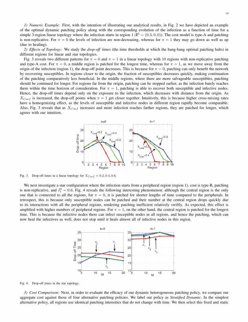
1) Numeric Example: First, with the intention of illustrating our analytical results, in Fig. 2 we have depicted an exampleof the optimal dynamic patching policy along with the corresponding evolution of the infection as a function of time for asimple 3-region linear topology where the infection starts in region 1 (I0 = (0.3, 0, 0)). The cost model is type-A and patchingis non-replicative. For π = 0 the levels of infection are non-decreasing, whereas for π = 1 they may go down as well as up(due to healing).

2) Effects of Topology: We study the drop-off times (the time thresholds at which the bang-bang optimal patching halts) indifferent regions for linear and star topologies.

Fig. 3 reveals two different patterns for π = 0 and π = 1 in a linear topology with 10 regions with non-replicative patchingand type-A cost. For π = 0, a middle region is patched for the longest time, whereas for π = 1, as we move away from theorigin of the infection (region 1), the drop-off point decreases. This is because for π = 0, patching can only benefit the networkby recovering susceptibles. In regions closer to the origin, the fraction of susceptibles decreases quickly, making continuationof the patching comparatively less beneficial. In the middle regions, where there are more salvageable susceptibles, patchingshould be continued for longer. For regions far from the origin, patching can be stopped earlier, as the infection barely reachesthem within the time horizon of consideration. For π = 1, patching is able to recover both susceptible and infective nodes.Hence, the drop-off times depend only on the exposure to the infection, which decreases with distance from the origin. AsXCoef is increased, the drop-off points when π = 1 get closer together. Intuitively, this is because higher cross-mixing rateshave a homogenizing effect, as the levels of susceptible and infective nodes in different region rapidly become comparable.Also, Fig. 3 reveals that as XCoef increases and more infection reaches farther regions, they are patched for longer, whichagrees with our intuition.

Fig. 3. Drop-off times in a linear topology for XCoef = 0.2, 0.4, 0.6.

We next investigate a star configuration where the infection starts from a peripheral region (region 1), cost is type-B, patchingis non-replicative, and I0

1 = 0.6. Fig. 4 reveals the following interesting phenomenon: although the central region is the onlyone that is connected to all the regions, for π = 0, it is patched for shorter lengths of time compared to the peripherals. Inretrospect, this is because only susceptible nodes can be patched and their number at the central region drops quickly dueto its interactions with all the peripheral regions, rendering patching inefficient relatively swiftly. As expected, this effect isamplified with higher numbers of peripheral regions. For π = 1, on the other hand, the central region is patched for the longesttime. This is because the infective nodes there can infect susceptible nodes in all regions, and hence the patching, which cannow heal the infectives as well, does not stop until it heals almost all of infective nodes in this region.

Fig. 4. Drop-off times in the star topology.

3) Cost Comparison: Next, in order to evaluate the efficacy of our dynamic heterogeneous patching policy, we compare ouraggregate cost against those of four alternative patching policies. We label our policy as Stratified Dynamic. In the simplestalternative policy, all regions use identical patching intensities that do not change with time. We then select this fixed and static

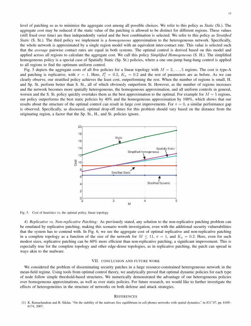
15

level of patching so as to minimize the aggregate cost among all possible choices. We refer to this policy as Static (St.). Theaggregate cost may be reduced if the static value of the patching is allowed to be distinct for different regions. These values(still fixed over time) are then independently varied and the best combination is selected. We refer to this policy as StratifiedStatic (S. St.). The third policy we implement is a homogeneous approximation to the heterogeneous network. Specifically,the whole network is approximated by a single region model with an equivalent inter-contact rate. This value is selected suchthat the average pairwise contact rates are equal in both systems. The optimal control is derived based on this model andapplied across all regions to calculate the aggregate cost. We call this policy Simplified Homogeneous (S. H.). The simplifiedhomogeneous policy is a special case of Spatially Static (Sp. St.) policies, where a one one-jump bang-bang control is appliedto all regions to find the optimum uniform control.

Fig. 5 depicts the aggregate costs of all five policies for a linear topology with M = 2, . . . , 5 regions. The cost is type-Aand patching is replicative, with π = 1. Here, I0

1 = 0.2, Ku = 0.2 and the rest of parameters are as before. As we canclearly observe, our stratified policy achieves the least cost, outperforming the rest. When the number of regions is small, H.and Sp. St. perform better than S. St., all of which obviously outperform St. However, as the number of regions increasesand the network becomes more spatially heterogeneous, the homogeneous approximation, and all uniform controls in general,worsen and the S. St. policy quickly overtakes them as the best approximation to the optimal. For example for M = 5 regions,our policy outperforms the best static policies by 40% and the homogeneous approximation by 100%, which shows that ourresults about the structure of the optimal control can result in large cost improvements. For π = 0, a similar performance gapis observed. Specifically, as discussed, optimal drop-off times for this problem should vary based on the distance from theoriginating region, a factor that the Sp. St., H., and St. policies ignore.

Fig. 5. Cost of heuristics vs. the optimal policy, linear topology.

4) Replicative vs. Non-replicative Patching: As previously stated, any solution to the non-replicative patching problem canbe emulated by replicative patching, making this scenario worth investigation, even with the additional security vulnerabilitiesthat the system has to contend with. In Fig. 6, we see the aggregate cost of optimal replicative and non-replicative patchingin a complete topology as a function of the size of the network for M ≤ 11, π = 1, and Ku = 0.2. Here, even for suchmodest sizes, replicative patching can be 60% more efficient than non-replicative patching, a significant improvement. This isespecially true for the complete topology and other edge-dense topologies, as in replicative patching, the patch can spread inways akin to the malware.

VII. CONCLUSION AND FUTURE WORK

We considered the problem of disseminating security patches in a large resource-constrained heterogeneous network in themean-field regime. Using tools from optimal control theory, we analytically proved that optimal dynamic policies for each typeof node follow simple threshold-based structures. We numerically demonstrated the advantage of our heterogeneous policiesover homogeneous approximations, as well as over static policies. For future research, we would like to further investigate theeffects of heterogeneities in the structure of networks on both defense and attack strategies.

REFERENCES

[1] K. Ramachandran and B. Sikdar, “On the stability of the malware free equilibrium in cell phones networks with spatial dynamics,” in ICC’07, pp. 6169–6174, 2007.

16

Fig. 6. Costs of replicative and non-replicative patching, complete topology.

[2] P. Wang, M. Gonzalez, C. Hidalgo, and A. Barabasi, “Understanding the spreading patterns of mobile phone viruses,” Science, vol. 324, no. 5930,p. 1071, 2009.

[3] Z. Zhu, G. Cao, S. Zhu, S. Ranjan, and A. Nucci, “A social network based patching scheme for worm containment in cellular networks,” in INFOCOM’09,pp. 1476–1484, IEEE, 2009.

[4] H. Leyden, “Blaster variant offers fix for pox-ridden pcs,” http://www.theregister.co.uk/2003/08/19/blaster variant offers fix/ , 2003.[5] M. Khouzani, S. Sarkar, and E. Altman, “Dispatch then stop: Optimal dissemination of security patches in mobile wireless networks,” in IEEE CDC’10,

pp. 2354–2359, 2010.[6] M. Khouzani, S. Sarkar, and E. Altman, “Optimal control of epidemic evolution,” in IEEE INFOCOM, 2011.[7] J. Mickens and B. Noble, “Modeling epidemic spreading in mobile environments,” in Proceedings of the 4th ACM Workshop on Wireless Security,

pp. 77–86, ACM, 2005.[8] K. Ramachandran and B. Sikdar, “Modeling malware propagation in networks of smart cell phones with spatial dynamics,” in IEEE INFOCOM’07,

pp. 2516–2520, 2007.[9] Z. Chen and C. Ji, “Spatial-temporal modeling of malware propagation in networks,” IEEE Transactions on Neural Networks, vol. 16, no. 5, pp. 1291–

1303, 2005.[10] F. Li, Y. Yang, and J. Wu, “CPMC: an efficient proximity malware coping scheme in smartphone-based mobile networks,” in IEEE INFOCOM’10,

pp. 1–9, 2010.[11] Y. Yang, S. Zhu, and G. Cao, “Improving sensor network immunity under worm attacks: a software diversity approach,” in Proceedings of the 9th ACM

international symposium on Mobile ad hoc networking and computing, pp. 149–158, ACM, 2008.[12] Y. Li, P. Hui, L. Su, D. Jin, and L. Zeng, “An optimal distributed malware defense system for mobile networks with heterogeneous devices,” SECON

2011, IEEE, pp. 1–9, 2011.[13] H. Nguyen and Y. Shinoda, “A macro view of viral propagation and its persistence in heterogeneous wireless networks,” in Fifth International Conference

on Networking and Services, pp. 359–365, IEEE, 2009.[14] M. Liljenstam, Y. Yuan, B. Premore, and D. Nicol, “A mixed abstraction level simulation model of large-scale internet worm infestations,” in 10th IEEE

International Symposium on Modeling, Analysis and Simulation of Computer and Telecommunications Systems, MASCOTS 2002, pp. 109–116, IEEE,2002.

[15] M. Faghani and H. Saidi, “Malware propagation in online social networks,” in 4th IEEE International Conference on Malicious and Unwanted Software(MALWARE), pp. 8–14, 2009.

[16] G. Zyba, G. Voelker, M. Liljenstam, A. Mehes, and P. Johansson, “Defending mobile phones from proximity malware,” in INFOCOM 2009, IEEE,pp. 1503–1511, IEEE, 2009.

[17] M. Altunay, S. Leyffer, J. Linderoth, and Z. Xie, “Optimal response to attacks on the open science grid,” Computer Networks, 2010.[18] G. Feichtinger, R. F. Hartl, and S. P. Sethi, “Dynamic optimal control models in advertising: recent developments,” Management Science, vol. 40, no. 2,

pp. 195–226, 1994.[19] S. P. Sethi, “Dynamic optimal control models in advertising: a survey,” SIAM review, vol. 19, no. 4, pp. 685–725, 1977.[20] S. P. Sethi and G. L. Thompson, Optimal control theory: applications to management science and economics, vol. 101. Kluwer Academic Publishers

Boston, 2000.[21] H. Behncke, “Optimal control of deterministic epidemics,” Optimal control applications and methods, vol. 21, no. 6, pp. 269–285, 2000.[22] K. Wickwire, “Mathematical models for the control of pests and infectious diseases: a survey,” Theoretical Population Biology, vol. 11, no. 2, pp. 182–238,

1977.[23] J. Cuzick and R. Edwards, “Spatial clustering for inhomogeneous populations,” Journal of the Royal Statistical Society. Series B (Methodological),

pp. 73–104, 1990.[24] W. Hsu and A. Helmy, “Capturing user friendship in WLAN traces,” IEEE INFOCOM poster, 2006.[25] T. Antunovic, Y. Dekel, E. Mossel, and Y. Peres, “Competing first passage percolation on random regular graphs,” ArXiv e-prints, 2011.[26] T. Kurtz, “Solutions of ordinary differential equations as limits of pure jump markov processes,” Journal of Applied Probability, pp. 49–58, 1970.[27] N. Gast, B. Gaujal, and J. Le Boudec, “Mean field for Markov decision processes: from discrete to continuous optimization,” Arxiv preprint

arXiv:1004.2342, 2010.[28] B. Bollobas, Modern graph theory, vol. 184. Springer Verlag, 1998.[29] R. F. Stengel, Optimal control and estimation. Dover, 1994.[30] M. Khouzani, S. Sarkar, and E. Altman, “Maximum damage malware attack in mobile wireless networks,” IEEE/ACM Transactions on Networking

(TON), vol. 20, no. 5, pp. 1347–1360, 2012.[31] P. Hui, A. Chaintreau, J. Scott, R. Gass, J. Crowcroft, and C. Diot, “Pocket switched networks and human mobility in conference environments,” in

ACM SIGCOMM Workshop on Delay-tolerant Networking, p. 251, ACM, 2005.[32] S. Eshghi, M. Khouzani, S. Sarkar, N. B. Shroff, and S. S. Venkatesh, “Optimal energy-aware epidemic routing in dtns.” Technical report, 2013. available

at http://www.seas.upenn.edu/ swati/TACoptimalenergyrouting.pdf.

17

APPENDIX APROOF OF THEOREM 1

We use the following general result :

Lemma 6. Suppose the vector-valued function f = (fi, 1 ≤ i ≤ 3M) has component functions given by quadratic formsfi(t,x) = xTQi(t)x+pi

Tx (t ∈ [0, T ]; x ∈ S), where S is the set of 3M -dimensional vectors x = (x1, . . . , x3M ) satisfyingx ≥ 0 and ∀j ∈ {1, . . . ,M};xj + xM+j + x2M+j = 1, Qi(t) is a matrix whose components are uniformly, absolutelybounded over [0, T ], as are the elements of the vector pi. Then, for an 3M -dimensional vector-valued function F, the systemof differential equations

F = f(t,F) (0 < t ≤ T )

subject to initial conditions F(0) ∈ S(34)

has a unique solution, F(t), which varies continuously with the initial conditions F0 ∈ S at each t ∈ [0, T ].

Proof: This lemma is virtually identical to Lemma 1 of [32] for N = 3M , with the difference that here fi(t,x) hasan additive pi

Tx term. Thus, we will only list the changes: As the Euclidean norm ‖Qi(t)x‖ is uniformly bounded over(t,x) ∈ [0, T ] × S, there exists C < ∞ such that sup[0,T ]×S ‖Qi(t)x‖ ≤ C. Also, ‖pi‖ ≤ H for some H < ∞ as all itselements are bounded. Now, for each t, we may write

fi(t,x)− fi(t,y) =(Qi(t)x + pi

)T(x− y) + (x− y)TQi(t)y

Taking absolute values of both sides, we obtain

|fi(t,x)− fi(t,y)| ≤∣∣(Qi(t)x)T (x− y)

∣∣+∣∣(x− y)TQi(t)y

∣∣+∣∣piT (x− y

)∣∣ ≤ (2C +H)‖x− y‖ (t ∈ [0, T ]; x,y ∈ S),

by using the triangle and Cauchy-Schwarz inequalities. Hence

‖f(t,x)− f(t,y)‖ ≤ L ‖x− y‖ (t ∈ [0, T ]; x,y ∈ S),

and so f(t, ·) is Lipschitz over S where the Lipschitz constant L = (2C +H)√

3M may be chosen uniformly for t ∈ [0, T ].The rest of the proof is exactly as in [32].Proof of Theorem 1: We write F(0) = F0, and in a slightly informal notation, F = F(t) = F(t,F0) to acknowledge the

dependence of F on the initial value F0.We first verify that S(t) + I(t) + R(t) = 1 for all t in both cases. By summing the left and right sides of the system

of equations (2) and the Ri equation that was left out (respectively the two sides of equations (5)), we see that in bothcases for all i,

(Si(t) + Ii(t) + Ri(t)

)= 0, and, in view of the initial normalization

(Si(0) + Ii(0) + Ri(0)

)= 1, we have(

Si(t) + Ii(t) +Ri(t))

= 1 for all t and all i.We now verify the non-negativity condition. Let F = (F1, . . . , F3M ) be the state vector in 3M dimensions whose elements

are comprised of (Si, 1 ≤ i ≤ M), (Ii, 1 ≤ i ≤ M) and (Ri, 1 ≤ i ≤ M) in some order. The system of equations (2) canthus be represented as F = f(t,F), where for t ∈ [0, T ] and x ∈ S, the vector-valued function f = (fi, 1 ≤ i ≤ 3M) hascomponent functions fi(t,x) = xTQi(t)x + pi

Tx in which (i) Qi(t) is a matrix whose non-zero elements are of the form±βjk, (ii) the elements of pi(t) are of the form ±βjkR0

juj and ±βjkπjkR0juj , whereas (5) can be represented in the same

form but with (i) Qi(t) having elements ±βjk, ±βjkuj , and ±βjkπjkuj , and (ii) pi = 0. Thus, the components of Qi(t)are uniformly, absolutely bounded over [0, T ]. Lemma 6 establishes that the solution F(t,F0) to the systems (2) and (5) isunique and varies continuously with the initial conditions F0; it clearly varies continuously with time. Next, using elementarycalculus, we show in the next paragraph that if F0 ∈ Int S (and, in particular, each component of F0 is positive), then eachcomponent of the solution F(t,F0) of (2) and (5) is positive at each t ∈ [0, T ]. Since F(t,F0) varies continuously with F0,therefore F(t,F0) ≥ 0 for all t ∈ [0, T ], F0 ∈ S, which completes the overall proof.

Accordingly, let the Si, Ii, and Ri component of F0 be positive. Since the solution F(t,F0) varies continuously with time,there exists a time, say t′ > 0, such that each component of F(t,F0) is positive in the interval [0, t′). The result followstrivially if t′ ≥ T . Suppose now that there exists t′′ < T such that each component of F(t,F0) is positive in the interval[0, t′′), and at least one such component is 0 at t′′.

We first examine the non-replicative case. We show that such components can not be Si for any i and subsequently ruleout Ii and Ri for all i. Note that uj(t), Ij(t), Sj(t) are bounded in [0, t′′] (recall (Sj(t) + Ij(t) +Rj(t)) = 1, Sj(t) ≥0, Ij(t) ≥ 0, Rj(t) ≥ 0 for all j ∈ {1, . . . ,M}, t ∈ [0, t′′]). From (2a) Si(t′′) = Si(0)e−

∫ t′′0

∑Mj=1(βjiIj(t)+βjiR

0juj(t)) dt.

Since all uj(t), Ij(t) are bounded in [0, t′′], Si(0) > 0, R0j ≥ 0, and βji, βji ≥ 0, therefore Si(t′′) > 0. Since Si(t) > 0,

Ii(t) ≥ 0 for all i, t ∈ [0, t′′], and βji ≥ 0, from (2b), Ii ≥ −Ii∑Mj=1 πjiβjiR

0juj for all i in the interval [0, t′′]. Thus,

Ii(t′′) ≥ Ii(0)e−

∫ t′′0

∑Mj=1 πji(βjiR

0juj(t)) dt. Since all uj(t), Ij(t), Sj(t) are bounded in [0, t′′], and Ii(0) > 0, βji, πji ≥ 0, it

follows that Ii(t′′) > 0 for all i ≥ 0. Finally, Ri(t′′) > 0 because Ri(0) > 0 and Ri(t) ≥ 0 from the above, so Ri(t) ≥ R0i ,

18

and Si(t) + Ii(t) ≤ 1− R0i for all t and i. This contradicts the definition of t′′ and in turn implies that F(t,F0) > 0 for all

t ∈ [0, T ], F0 ∈ Int S.The proof for the replicative case is similar, with the difference that R0

i is replaced with Ri, which is itself bounded.Since the control and the unique state solution S(t), I(t) are non-negative, (2a, 5a) imply that S(t) is a non-increasing

function of time. Thus, Sj(t) = 0 if Sj(0) = 0 for any j. Using the argument in the above paragraph and starting from at′ ∈ [0, T ) where Sj(t′) > 0, Ij(t′) > 0, or Rj(t′) > 0, it may be shown respectively that Sj(t) > 0, Ij(t) > 0, and Rj(t) > 0for all t > t′. All that remains to show now is:

Lemma 7. There exists ε > 0 such that I(t) > 0 for t ∈ (0, ε).

Let d(i, j) be the distance from type j to type i (i.e., for all i, d(i, i) = 0 and for all pairs (i, j), d(i, j) = 1+ minimumnumber of types in a path from type j to type i). Now, define d(i, U) := minj∈U d(i, j), where U := { i : I0

i > 0 }. Since weassumed that every type i is either in U or is connected to a type in U , d(i, U) < M for all types i.

Let δ > 0 be a time such that for all types i such that d(i, U) = 0 (the initially infected types), we have Ii(t) > 0 fort ∈ [0, δ). Thus, proving Lemma 8 below will be equivalent to proving Lemma 7, given an appropriate scaling of δ.

Lemma 8. For all i and for all integers r ≥ 0, if d(i, U) ≤ r, then Ii(t) > 0 for t ∈ ( rM δ, T ).

Proof: By induction on r.Base case: r = 0. If d(i, U) = 0, this means that the type is initially infected, and thus Ii(t) > 0 for t ∈ (0, T ) by definition.

Therefore the base case holds.Induction step: Assume that the statement holds for r = 0, . . . , k and consider r = k + 1. Since (k+1

M δ, T ) ⊂ ( kM δ, T ),we need to examine types i such that d(i, U) = k + 1. In equation (2b) at t = k+1

M δ, the first sum on the right involvesterms like Ij(k+1

M δ)Si(k+1M δ) where j is a neighbor of i, while the second sum involves terms like Ii(k+1

M δ)uj(k+1M δ). Since

d(i, U) = k+1, there exist neighbours j of i such that d(j, U) = k, and therefore Ij(t) > 0 for t ∈ [k+1M δ, T ) (by the induction

hypothesis). Hence since S0i > 0 and βji > 0 (i and j being neighbours), for such t, Ii(t) > −Ii(t)

∑Mj=1 πjiβjiR

0juj(t) ≥

−GIi(t), where G ≥ 0 is an upperbound on the sum (continuous functions are bounded on a closed and bounded interval).Thus Ii(t) > Ii(

k+1M δ)e−Kt > 0, completing the proof for r = k + 1.