1

Monopsony

Monopsony is a situation where there is one buyer – you have seen Monopoly, a case of

one seller. Here we want to explore the impact on the market when there is only one

buyer of labor.

2

Up to now in our studies we have assumed

-firms are price takers in the output market – meaning the price is set in the market by the interaction of many buyers and sellers and then any one firm just works with the market price,

-firms are wage takers in the input market – meaning the wage is set in a market setting as well.

Here we have the situation of a single buyer of labor and because of this the firm has the ability to set the wage instead of take the wage.

Let’s start with a nondiscriminating monopsonist. Recall that suppliers of labor have an upward sloping supply of labor curve (ignoring the backward bending case). In fact we take as given the market supply of labor as the sum of the labor supply from many individuals. On the next slide I have an example.

3

$

E

Wage E

4 0

5 1

6 2

7 3

8 4

1 2 3 4

8765

S

In this example the suppliers of labor will supply an E of 1 when the wage is 5, and so on.

4

$

E

Wage E TLC MLC

4 0 0 xxx

5 1 5 5

6 2 12 7

7 3 21 9

8 4 32 11

1 2 3 4

8765

S

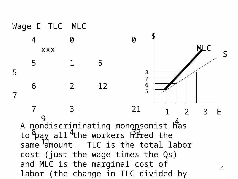
A nondiscriminating monopsonist has to pay all the workers hired the same amount. TLC is the total labor cost (just the wage times the E) and MLC is the marginal cost of labor (the change in TLC divided by the change in labor supplied Qs).

MLC

5

Note, in order to get two units of labor the firm would have to pay 12 6 to each worker. But the first worker would have worked for 5. So the marginal cost to the firm of the second worker is 7, which is the 6 to get the second worker but includes the 1 you give to the first worker. A similar story holds for all future units of labor.

The point here is that from the point of view of the firm the MLC curve is not the supply of labor curve. The MLC curve is above the supply of labor curve. The MLC curve is the curve that shows the change in total labor cost from having additional units of labor. The curve will be used to think about how much labor the firm would want to hire. The other piece of information here is to remember that the demand for labor curve was the value of the marginal product of labor curve. It deals with the revenue of additional workers.

6

Employment or hiring decision by the firm

The profit maximizing nondiscriminating monopsonist will hire labor up to the point where the value of the marginal product equals the MLC. Recall the value of marginal product is the revenue generated by the additional worker.

The wage paid to each worker is the wage on the supply curve at the optimal quantity.

On the next screen I have the result in a graph.

7

$

E

S

MLC

VMP = D

W1

E1

8

The firm on the previous screen does not want to go past the employment level where the VMP = MLC because those workers would bring in less revenue than the cost to hire them and thus the firm would lose out on some profit.

Plus the firm would not want to stop short of this point because they would not take units of labor where the revenues of the labor are greater than the costs of taking the labor.

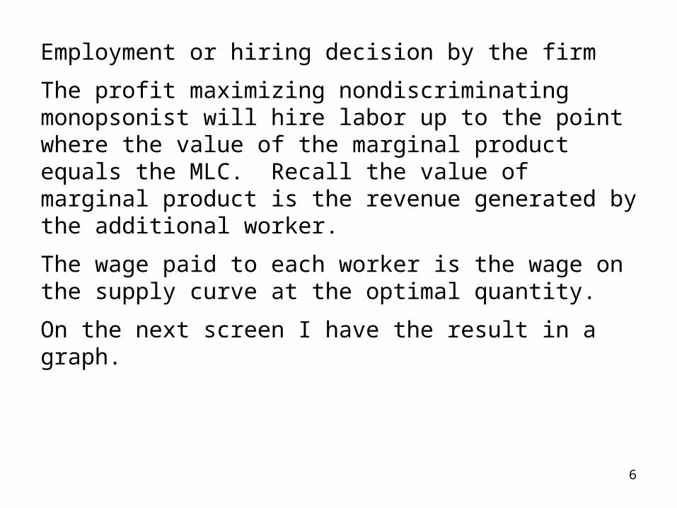
On the next slide we compare the result of monopsony with that of competition. In competition the wage and quantity traded occur where the supply and demand are equal.

9

$

L

S

MLC

VMP = D

W1

L1 Lc

Wc

10

The monopsony pays a lower wage than in competition and hires less labor.

Remember a monopsony is a single buyer of labor. Often in economics we see that if the demand or supply side of the market has only 1 player then the single actor has market power. The market power often results in less than desirable outcomes. Here the single buyer uses power to pay lower wages and thus fewer folks want to work at that low wage.

The monopsony likes this outcome better than competition but not everyone else. Workers get lower wages and less work and since less labor is desired less output is made – output people probably want.

11

Note here that the monopsony pays the workers less than there VMP –> W <VMP. In this sense it has been said the monopsony exploits the workers.

12

More Monopsony

13

On the next slide I have reproduced something from a previous section. Note the marginal labor cost is greater than the wage at each labor amount because in order to get more labor the firm would have to pay all workers the higher amount. Thus the MLC at a labor amount reflects both the increased cost from the additional worker and the additional amount that each of the previous workers would get.

For example, with two workers the marginal labor cost is 7. This is made up of the 6 for the 2nd worker and the first worker would get 6 instead of 5 that the first worker would have gotten if only one worker was taken.

14

$

E

Wage E TLC MLC

4 0 0 xxx

5 1 5 5

6 2 12 7

7 3 21 9

8 4 32 11

1 2 3 4

8765

S

A nondiscriminating monopsonist has to pay all the workers hired the same amount. TLC is the total labor cost (just the wage times the Qs) and MLC is the marginal cost of labor (the change in TLC divided by the change in labor supplied Qs).

MLC

15

Now, say a minimum wage is enacted at $7 per hour. I have reproduced the table from before and put in parentheses the new values for TLC and MLC. I kept the wage column the same, although you could probably argue to make any wage below the minimum that wage.

Wage E TLC MLC 4 0 0 xxx 5 1 5 (7) 5 (7) 6 2 12 (14) 7 (7) 7 3 21 (21) 9 (7) 8 4 32 (32) 11 (11)What the minimum wage does is change the MLC to a constant at 7 for all those units of labor that would have been supplied at wages of 7 or less.

16

$

E

In the graph at the right you see the old MLC curve as the thin line. The new MLC curve is horizontal at the minimum wage. When labor supply is 3 the MLC curve is vertical and after that the MLC curve follows the old MLC.

1 2 3 4

8765

S

So, in general, with a minimum wage the MLC is horizontal at the minimum wage until you get to the supply line, from there it becomes vertical, and after that it follows the original MLC line.

MLC

17

$

E

S

MLC

VMP = D

W1

E1 Ec

Wc

Case 1 E’

18

Case 1 Say the minimum wage enacted in a monopsony market is below what would be in the market with competition, but above the monopsony wage.

Here the firm would want the labor amount E’ because that is where VMP = MLC and if it pays the minimum wage that many workers will work. Thus the equilibrium wage is the minimum wage and the equilibrium amount traded would be E’.

So, this type of minimum wage can actually make employment go up – no unemployment from a minimum wage!

19

$

E

S

MLC

VMP = D

W1

E1 Ec

Wc

Case 2 E’

unemployment

E’’

20

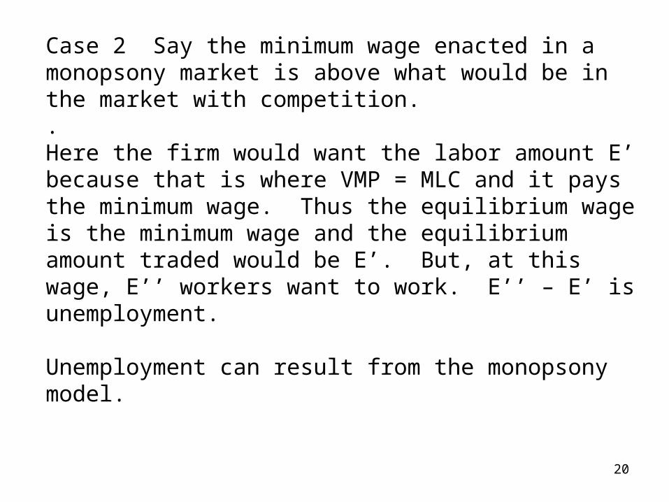
Case 2 Say the minimum wage enacted in a monopsony market is above what would be in the market with competition..Here the firm would want the labor amount E’ because that is where VMP = MLC and it pays the minimum wage. Thus the equilibrium wage is the minimum wage and the equilibrium amount traded would be E’. But, at this wage, E’’ workers want to work. E’’ – E’ is unemployment.

Unemployment can result from the monopsony model.

21

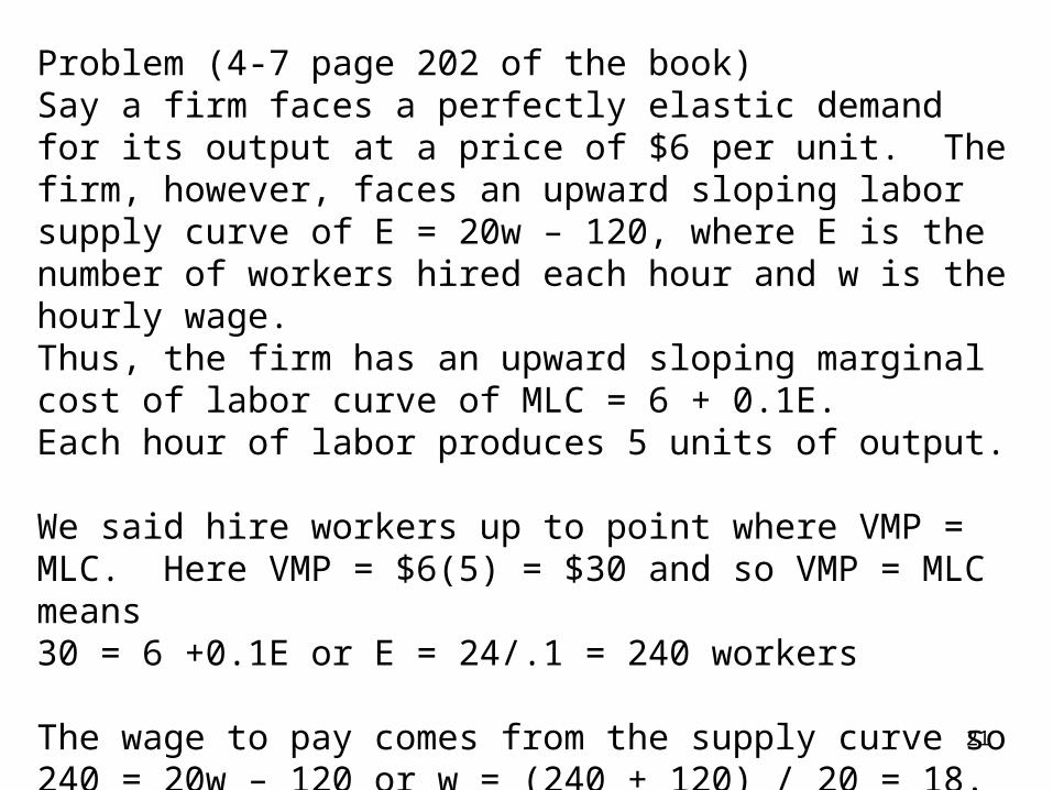
Problem (4-7 page 202 of the book)Say a firm faces a perfectly elastic demand for its output at a price of $6 per unit. The firm, however, faces an upward sloping labor supply curve of E = 20w – 120, where E is the number of workers hired each hour and w is the hourly wage.Thus, the firm has an upward sloping marginal cost of labor curve of MLC = 6 + 0.1E.Each hour of labor produces 5 units of output.

We said hire workers up to point where VMP = MLC. Here VMP = $6(5) = $30 and so VMP = MLC means30 = 6 +0.1E or E = 24/.1 = 240 workers

The wage to pay comes from the supply curve so 240 = 20w – 120 or w = (240 + 120) / 20 = 18. Profit = revenue minus cost = $6(5)240 – 18(240) = $2880