1

MF-852 Financial Econometrics

Lecture 3

Review of Probability

Roy J. EpsteinFall 2003

2

So Far We Have Seen That… Excel does all of our matrix number crunching. We can solve basic optimization (maximize,

minimize) problems with constraints in Excel. We can find the coefficients in the linear

regression model (that is, predict y in terms of the x’s and an error term):

y = 0 + 1x1 + 2x2 + … + nxn + e

Write the equation as y = X + e.

Solution is = (XX) –1 Xy (Excel does this automatically with regression function in Tools-Data Analysis)

3

Probability and Statistics We can always calculate the

regression coefficients.

But how reliable are they? Remember last time that more bedrooms

caused lower prices in the regression!

Probability and statistics are used to determine reliability of a data analysis.

4

Sample Spaces and Events The sample space S defines the

possible outcomes of an experiment. Coin flip: the sample space has two

outcomes, heads (H) and tails (T). S = {H, T}

Any given collection of outcomes in the sample space constitutes a possible event E. H is an event.

5

Sample Spaces, cont. Sample spaces can be large.

3 coin flips: S = {HHH, HTH, HHT, HTT, THH, TTH,

THT, TTT} Events can be complex.

2 heads is an event in S E = {HTH, HHT, THH}.

6

Probability

With the 3-coin flip, S has eight outcomes.

E = {HTH, HHT, THH} therefore has probability 3/8.

P(E) = 0.375.

7

Independent Events Consider E1 and E2 defined on S.

P(E1) = p1, P(E2) = p2

Probability of E2 given that E1 has occurred is written P(E2|E1). Called conditional probability.

If P(E2|E1) = P(E2) then E2 and E1 are independent events.

8

Independence When two events A and B are

independent, then knowledge that A occurred (or will occur) does not provide information about whether B occurred (or will occur).

9

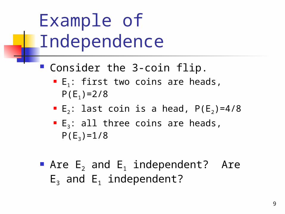
Example of Independence Consider the 3-coin flip.

E1: first two coins are heads, P(E1)=2/8

E2: last coin is a head, P(E2)=4/8 E3: all three coins are heads,

P(E3)=1/8

Are E2 and E1 independent? Are E3 and E1 independent?

10

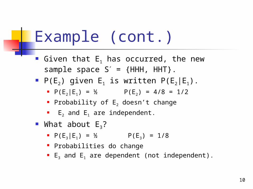
Example (cont.) Given that E1 has occurred, the new

sample space S = {HHH, HHT}. P(E2) given E1 is written P(E2|E1).

P(E2|E1) = ½ P(E2) = 4/8 = 1/2 Probability of E2 doesn’t change E2 and E1 are independent.

What about E3? P(E3|E1) = ½ P(E3) = 1/8 Probabilities do change E3 and E1 are dependent (not independent).

11

Independence and Probability of Intersection of Events Intersection: joint occurrence of

E1 and E2 defined on S. Written as E1 E2

If P(E1 E2) = P(E1) P(E2) then the events are independent.

12

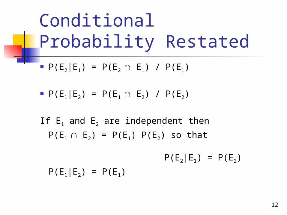
Conditional Probability Restated P(E2|E1) = P(E2 E1) / P(E1)

P(E1|E2) = P(E1 E2) / P(E2)

If E1 and E2 are independent then

P(E1 E2) = P(E1) P(E2) so that P(E2|E1) = P(E2)

P(E1|E2) = P(E1)

13

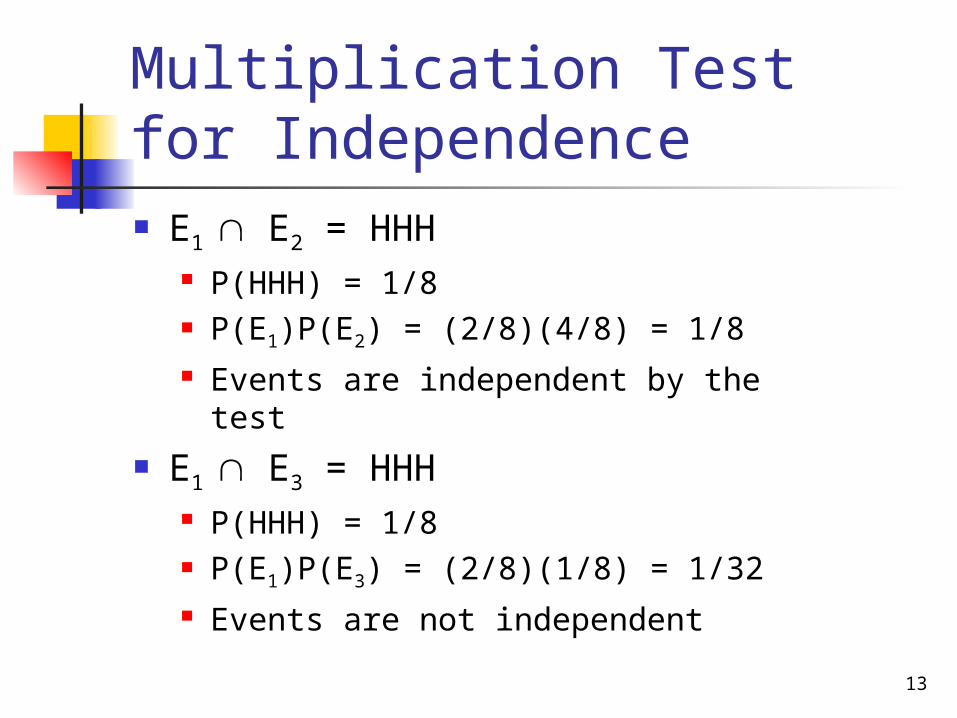
Multiplication Test for Independence E1 E2 = HHH

P(HHH) = 1/8 P(E1)P(E2) = (2/8)(4/8) = 1/8 Events are independent by the test

E1 E3 = HHH P(HHH) = 1/8 P(E1)P(E3) = (2/8)(1/8) = 1/32 Events are not independent

14

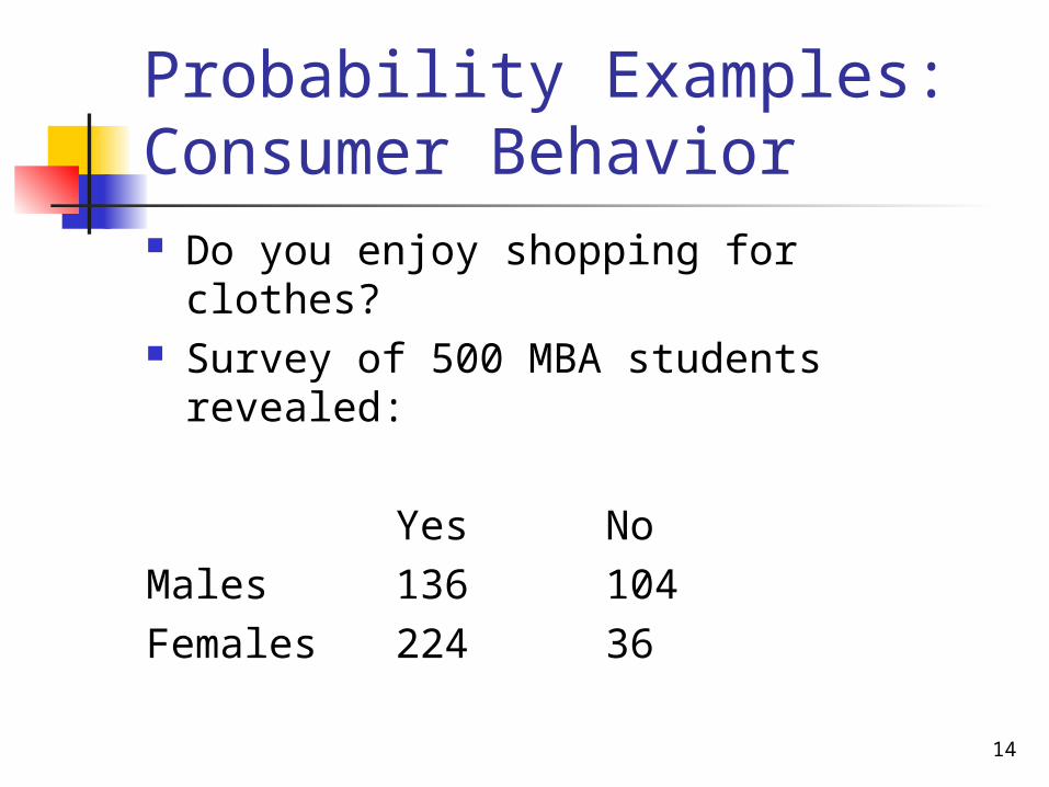
Probability Examples: Consumer Behavior Do you enjoy shopping for

clothes? Survey of 500 MBA students

revealed:

Yes NoMales 136 104Females 224 36

15

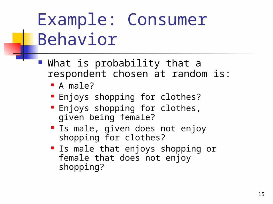
Example: Consumer Behavior What is probability that a

respondent chosen at random is: A male? Enjoys shopping for clothes? Enjoys shopping for clothes, given

being female? Is male, given does not enjoy

shopping for clothes? Is male that enjoys shopping or

female that does not enjoy shopping?

16

Example: Consumer Behavior Is enjoyment of shopping for

clothes independent of gender? Use multiplication test.

17

Independence: Intuition When 2 events are independent,

then information about one event provides no information about the other.

Essential concept in building a statistical model. Joint probabilities can be calculated by

simple multiplication. If any unused information is

independent of the problem under study then the model is “efficient,” i.e., makes best use of the data.

18

Random Variables A random variable is a function

defined on the sample space that summarizes events of interest.

3-coin flip: the number of heads in the 3 flips is a random variable.

The random variable takes on different values, each with a probability determined by the underlying sample space.

19

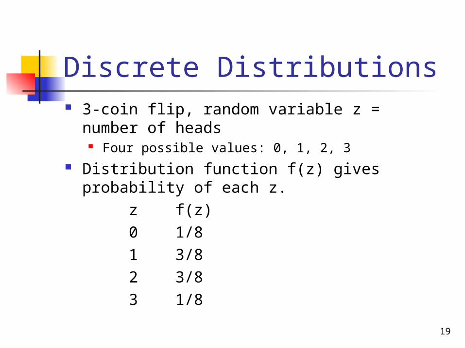
Discrete Distributions 3-coin flip, random variable z = number

of heads Four possible values: 0, 1, 2, 3

Distribution function f(z) gives probability of each z.

z f(z)0 1/81 3/82 3/83 1/8

20

Discrete Distributions Everyone in class should now flip

a coin 3 times. Let’s construct an empirical

frequency distribution for the number of heads!

21

Discrete Distributions Note that for a probability

distribution: 0 f(zi) 1 (negative probability

and probability greater than 1 makes no sense)

∑ f(zi) = 1 (all the different outcomes must sum to 1 in probability)

22

Expected Value Let z be a random variable with

distribution f(z). The expected value of z is

denoted E(z) or z or just if the context is clear. Also called mean value or the mean

Expected value = ∑zf(z). weighted average of z, where the

probabilities are the weights.

23

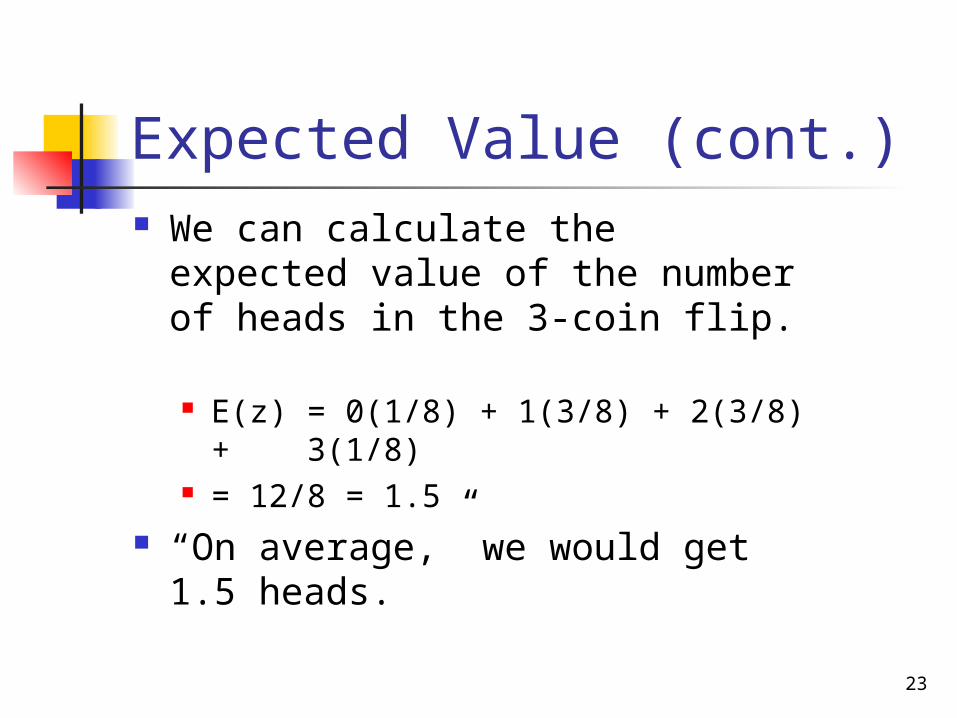
Expected Value (cont.) We can calculate the expected

value of the number of heads in the 3-coin flip. E(z) = 0(1/8) + 1(3/8) + 2(3/8) +

3(1/8) = 12/8 = 1.5

“On average,” we would get 1.5 heads.

24

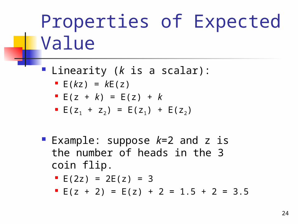
Properties of Expected Value Linearity (k is a scalar):

E(kz) = kE(z) E(z + k) = E(z) + k E(z1 + z2) = E(z1) + E(z2)

Example: suppose k=2 and z is the number of heads in the 3 coin flip. E(2z) = 2E(z) = 3 E(z + 2) = E(z) + 2 = 1.5 + 2 = 3.5

25

Properties of Expected Value Average deviation of a random

variable from its expected value is zero: E(z – z) = ∑zf(z) – ∑zf(z) = z – z∑f(z) = z – z = 0

Since “on average” a random variable equals its expected value, the average deviation from the mean is 0!

26

A Card Game with Monte Hall

We will play in class.

27

Variance Variance is the expected value of

the square of the deviation of a random variable from its mean. Var(z) = 2 = E[(z – z)2] = ∑(z2 – 2zz + ∑z

2)f(z) = ∑(z2)f(z) – 2z∑zf(z) + z

2

= ∑(z2)f(z) – 2z∑zf(z) + z2

= ∑(z2)f(z) –z2

28

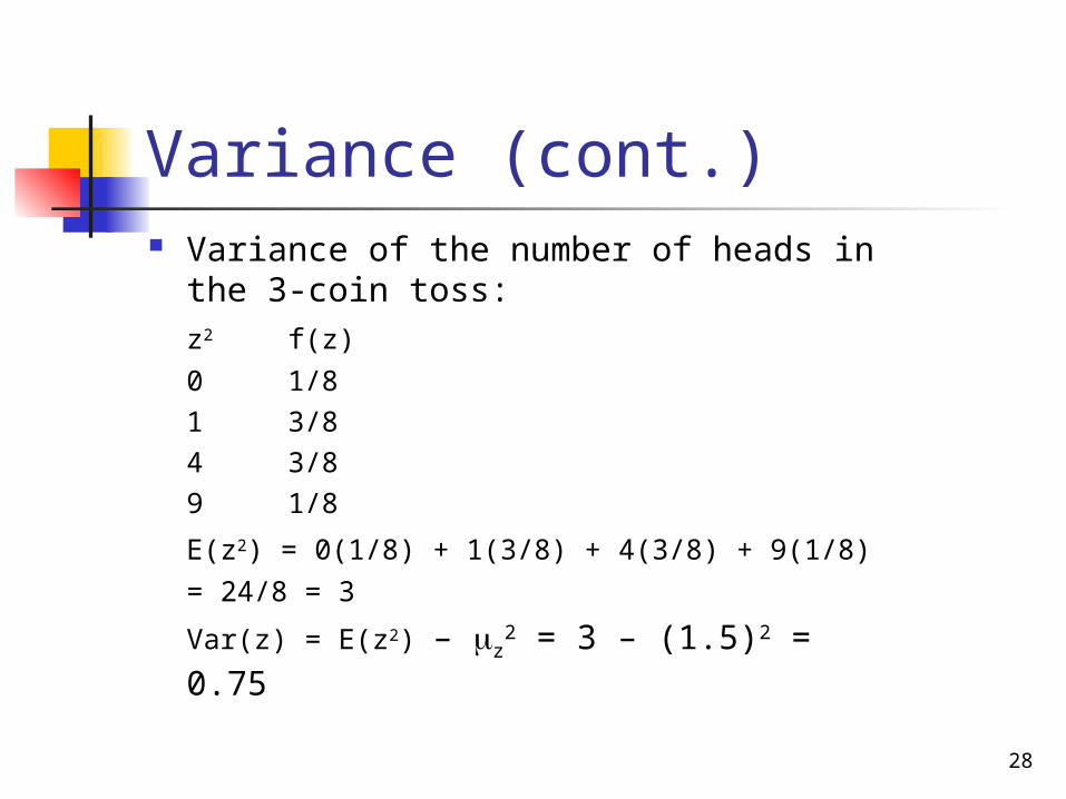
Variance (cont.) Variance of the number of heads in the

3-coin toss:z2 f(z)

0 1/81 3/84 3/89 1/8

E(z2) = 0(1/8) + 1(3/8) + 4(3/8) + 9(1/8)

= 24/8 = 3

Var(z) = E(z2) – z2 = 3 – (1.5)2 = 0.75

29

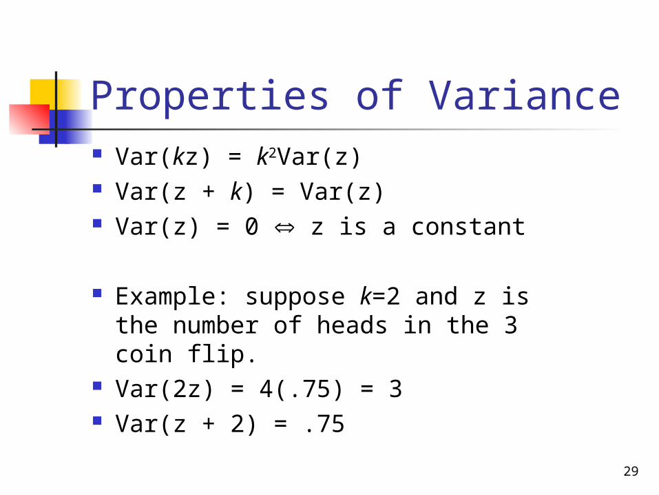
Properties of Variance Var(kz) = k2Var(z) Var(z + k) = Var(z) Var(z) = 0 z is a constant

Example: suppose k=2 and z is the number of heads in the 3 coin flip.

Var(2z) = 4(.75) = 3 Var(z + 2) = .75

30

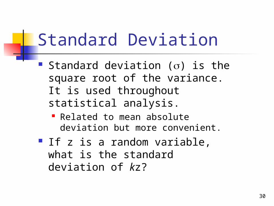
Standard Deviation Standard deviation () is the

square root of the variance. It is used throughout statistical analysis. Related to mean absolute deviation

but more convenient. If z is a random variable, what is

the standard deviation of kz?

31

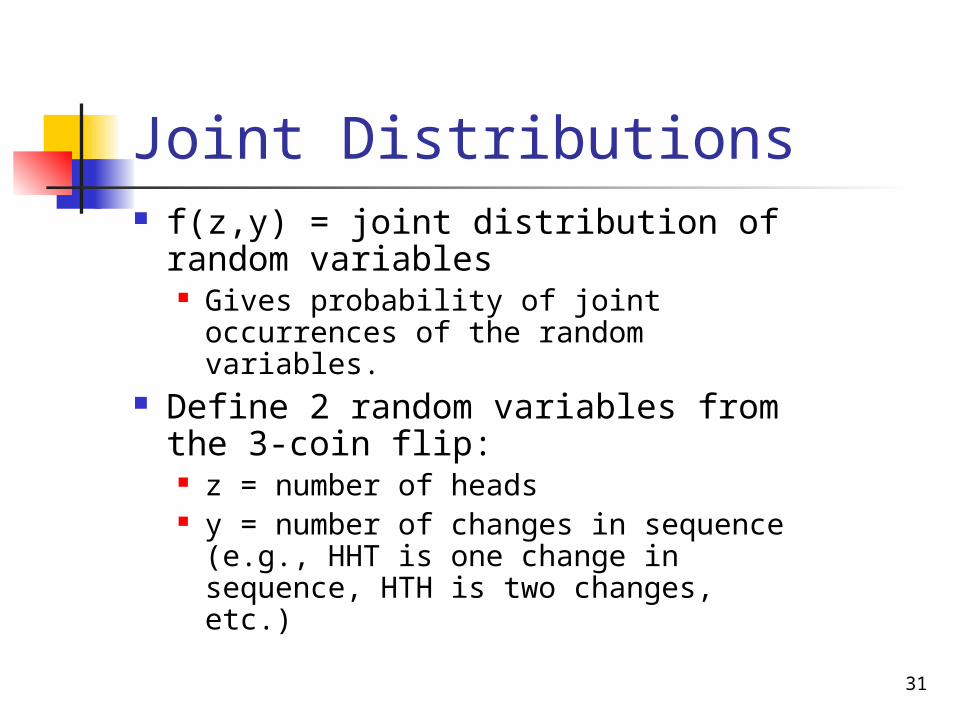
Joint Distributions f(z,y) = joint distribution of

random variables Gives probability of joint occurrences

of the random variables. Define 2 random variables from

the 3-coin flip: z = number of heads y = number of changes in sequence

(e.g., HHT is one change in sequence, HTH is two changes, etc.)

32

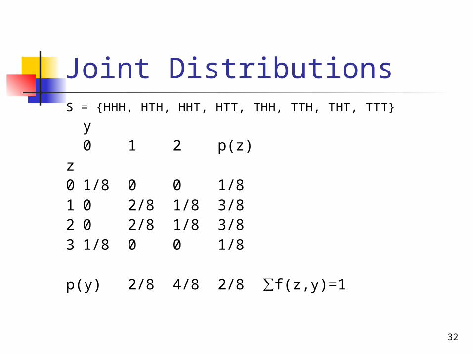
Joint DistributionsS = {HHH, HTH, HHT, HTT, THH, TTH, THT, TTT}

y0 1 2 p(z)

z0 1/8 0 0 1/81 0 2/8 1/8 3/82 0 2/8 1/8 3/83 1/8 0 0 1/8

p(y) 2/8 4/8 2/8 ∑f(z,y)=1

33

Covariance Random variables y and z have

positive covariance if: On average, when y is above (below)

its mean then z is also above (below) its mean.

Negative covariance: On average, when y is above (below)

its mean then z is below (above) its mean.

34

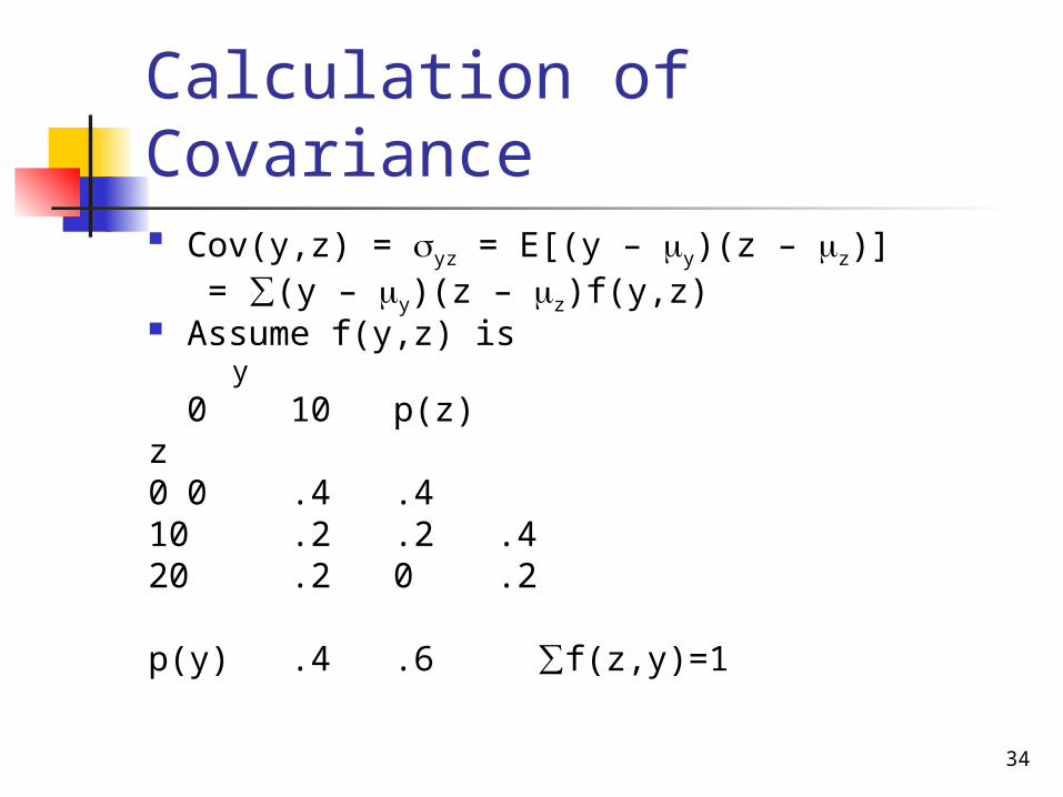
Calculation of Covariance Cov(y,z) = yz = E[(y – y)(z – z)]

= ∑(y – y)(z – z)f(y,z) Assume f(y,z) is

y0 10 p(z)

z0 0 .4 .410 .2 .2 .420 .2 0 .2

p(y) .4 .6 ∑f(z,y)=1

35

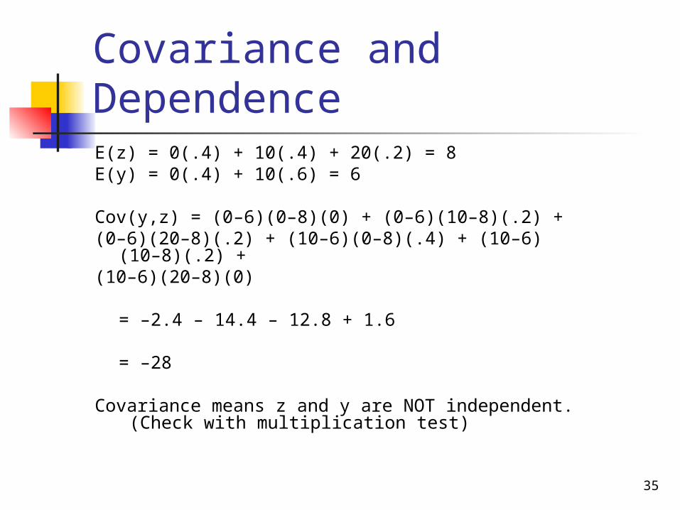
Covariance and DependenceE(z) = 0(.4) + 10(.4) + 20(.2) = 8E(y) = 0(.4) + 10(.6) = 6

Cov(y,z) = (0–6)(0–8)(0) + (0–6)(10–8)(.2) + (0–6)(20–8)(.2) + (10–6)(0–8)(.4) + (10–6)(10–8)

(.2) + (10–6)(20–8)(0)

= –2.4 – 14.4 – 12.8 + 1.6

= –28 Covariance means z and y are NOT independent.

(Check with multiplication test)

36

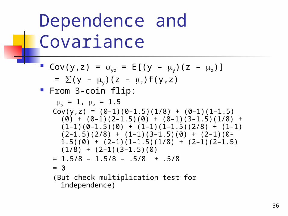
Dependence and Covariance Cov(y,z) = yz = E[(y – y)(z – z)]

= ∑(y – y)(z – z)f(y,z) From 3-coin flip:

y = 1, z = 1.5Cov(y,z) = (0–1)(0–1.5)(1/8) + (0–1)(1–1.5)(0) +

(0–1)(2–1.5)(0) + (0–1)(3–1.5)(1/8) + (1–1)(0–1.5)(0) + (1–1)(1–1.5)(2/8) + (1–1)(2–1.5)(2/8) + (1–1)(3–1.5)(0) + (2–1)(0–1.5)(0) + (2–1)(1–1.5)(1/8) + (2–1)(2–1.5)(1/8) + (2–1)(3–1.5)(0)

= 1.5/8 – 1.5/8 – .5/8 + .5/8= 0(But check multiplication test for independence)

37

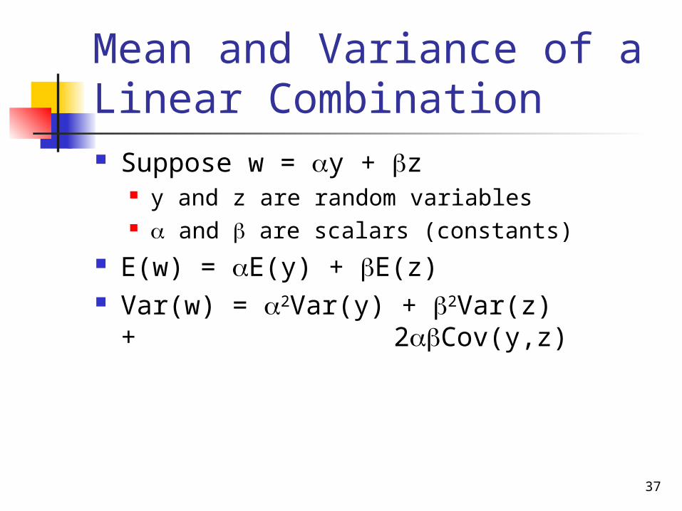
Mean and Variance of a Linear Combination Suppose w = y + z

y and z are random variables and are scalars (constants)

E(w) = E(y) + E(z) Var(w) = 2Var(y) + 2Var(z) +

2Cov(y,z)

38

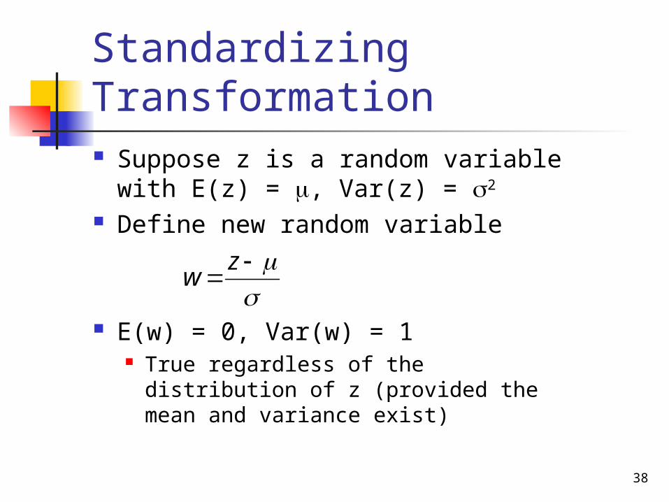
Standardizing Transformation Suppose z is a random variable

with E(z) = , Var(z) = 2

Define new random variable

E(w) = 0, Var(w) = 1 True regardless of the distribution of

z (provided the mean and variance exist)

z

w

39

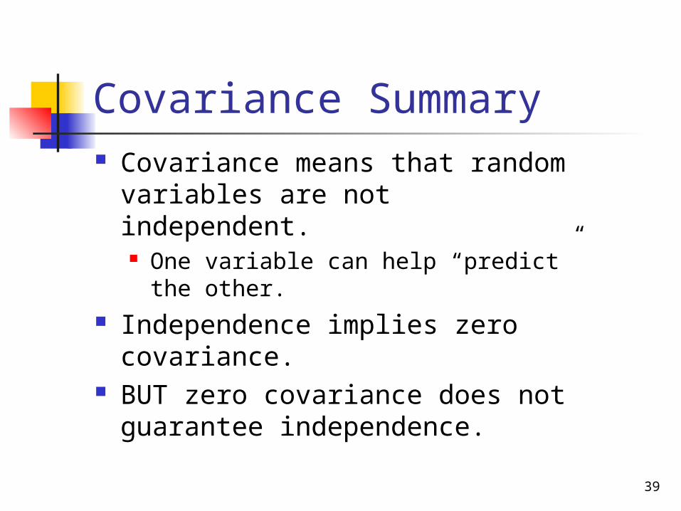
Covariance Summary Covariance means that random

variables are not independent. One variable can help “predict” the

other. Independence implies zero

covariance. BUT zero covariance does not

guarantee independence.

40

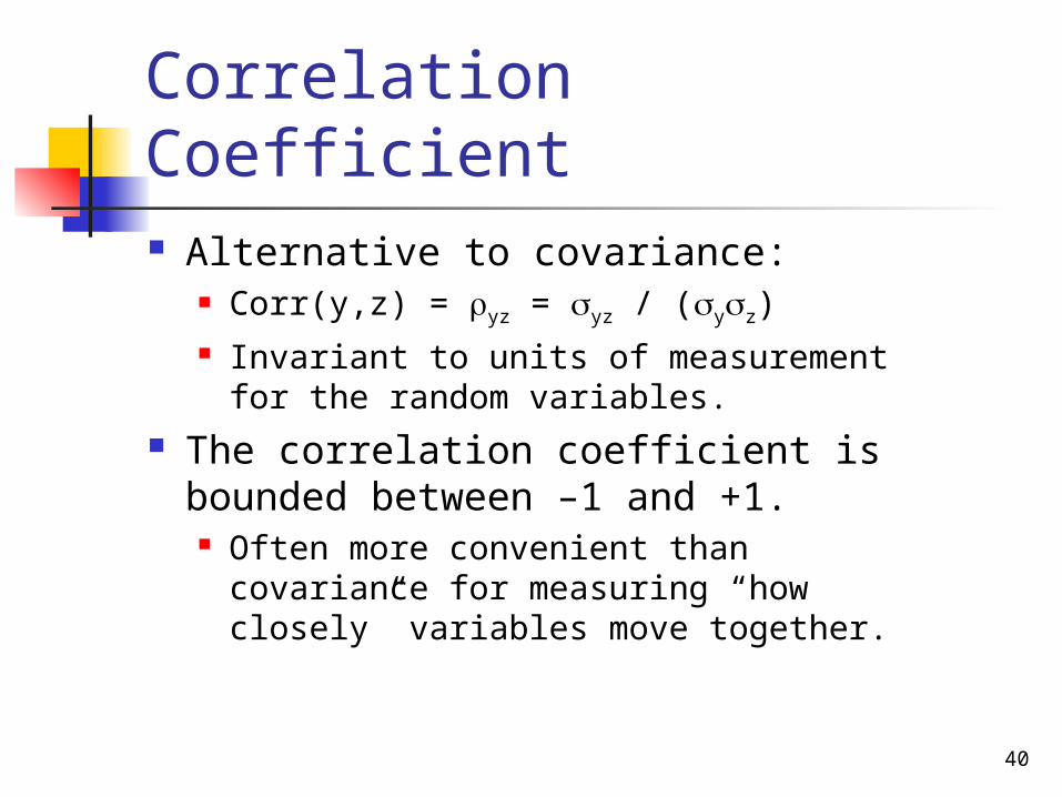
Correlation Coefficient Alternative to covariance:

Corr(y,z) = yz = yz / (yz) Invariant to units of measurement

for the random variables. The correlation coefficient is

bounded between –1 and +1. Often more convenient than

covariance for measuring “how closely” variables move together.

41

Calculation of Correlation Coefficient Assume f(y,z) is

y

0 10 p(z)z0 0 .4 .410 .2 .2 .420 .2 0 .2

p(y) .4 .6 ∑f(z,y)=1

42

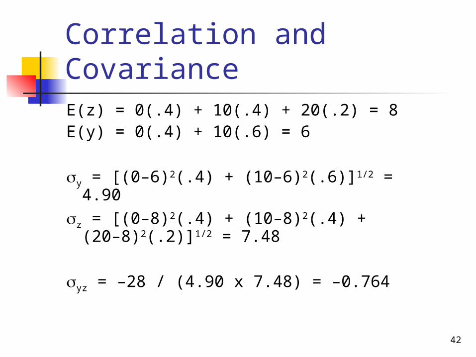
Correlation and CovarianceE(z) = 0(.4) + 10(.4) + 20(.2) = 8E(y) = 0(.4) + 10(.6) = 6

y = [(0–6)2(.4) + (10–6)2(.6)]1/2 = 4.90

z = [(0–8)2(.4) + (10–8)2(.4) + (20–8)2(.2)]1/2 = 7.48

yz = –28 / (4.90 x 7.48) = –0.764

43

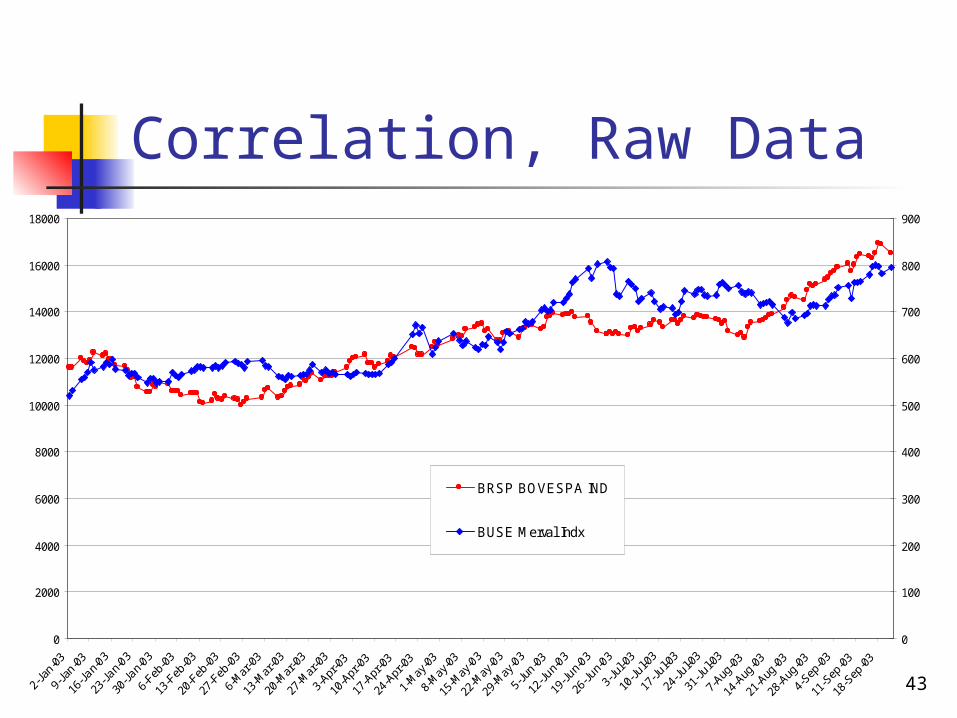
Correlation, Raw Data

0

2000

4000

6000

8000

10000

12000

14000

16000

18000

0

100

200

300

400

500

600

700

800

900

BRSP BOVESPA IND

BUSE Merval Indx

44

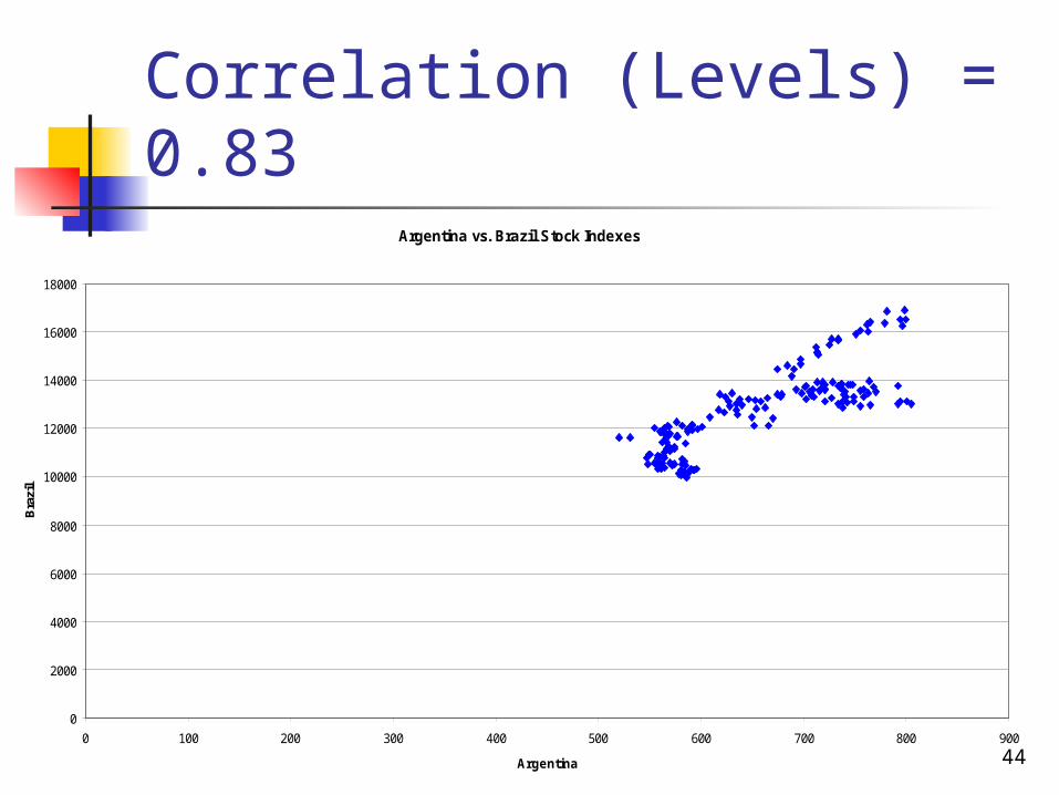
Correlation (Levels) = 0.83Argentina vs. Brazil Stock Indexes

0

2000

4000

6000

8000

10000

12000

14000

16000

18000

0 100 200 300 400 500 600 700 800 900

Argentina

Bra

zil

45

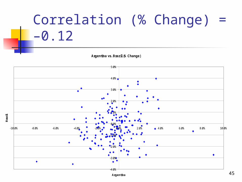
Correlation (% Change) = –0.12

Argentina vs. Brazil (% Change)

-4.0%

-3.0%

-2.0%

-1.0%

0.0%

1.0%

2.0%

3.0%

4.0%

5.0%

-10.0% -8.0% -6.0% -4.0% -2.0% 0.0% 2.0% 4.0% 6.0% 8.0% 10.0%

Argentina

Bra

zil