Tanagra 

21/01/09    1/26 

1 Introduction

Computing a Gain Chart. Comparing  the computation  time of data mining  tools on a  large dataset under 

Linux. 

The gain chart is an alternative to confusion matrix for the evaluation of a classifier.  Its name is sometimes 

different  according  the  tools  (e.g.  lift  curve,  lift  chart,  cumulative  gain  chart,  etc.).  The main  idea  is  to 

elaborate a scatter plot where the X coordinates  is the percent of the population and the Y coordinates  is 

the  percent  of  the  positive  value  of  the  class  attribute.  The  gain  chart  is  used mainly  in  the marketing 

domain where we want to detect potential customers, but it can be used in other situations. 

The  construction  of  the  gain  chart  is  already  outlined  in  a  previous  tutorial  (see  http://data‐mining‐

tutorials.blogspot.com/2008/11/lift‐curve‐coil‐challenge‐2000.html).  In  this  tutorial,  we  extend  the 

description to other data mining tools (Knime, RapidMiner, Weka and Orange). The second originality of this 

tutorial  is  that we  lead  the  experiment  under  Linux  (French  version  of Ubuntu  8.10  –  see  http://data‐

mining‐tutorials.blogspot.com/2009/01/tanagra‐under‐linux.html  for  the  installation  and  the  utilization  of 

Tanagra under Linux). The third originality is that we handle a large dataset with 2.000.000 examples and 

41 variables. It will be very interesting to study the behavior of these tools in this configuration, especially 

because our computer is not really powerful (Celeron, 2.53 GHz, 1 MB RAM). 

 

We adopt the same way for each tool. In a first time, we define the sequence of operations and the settings 

Tanagra 

21/01/09    2/26 

on a sample of 2.000 examples. Then,  in a second time, we modify the data source, we handle the whole 

dataset. We measure the computation time and the memory occupation. We note that some tools failed 

the analysis on the complete dataset. 

About  the  learning method, we  use  a  linear  discriminant  analysis with  a  variable  selection  process  for 

Tanagra. For  the other  tools,  this approach  is not available. So, we use a Naive Bayes method which  is a 

linear classifier also. 

2 Dataset

We use a modified version of the KDD‐CUP 99 dataset. The aim of the analysis is the detection of a network 

intrusion  (http://kdd.ics.uci.edu/databases/kddcup99/kddcup99.html).    We  want  to  detect  a  normal 

connection  (binary problem  "normal network  connection or not").   More precisely, we ask  the  following 

problem: "if we set a score to examples and rank them according to this score, what  is the proportion of 

positive (normal) connection detected if we select only 20 percent of the whole connections?" 

We have two data files. The first contains 2.000.000 examples  (full_gain_chart.arff).  It  is used to compare 

the  ability  of  the  tools  to  handle  a  large  dataset.  The  second  is  a  sample  with  2.000  examples 

(sample_gain_chart.arff). It is used for specifying all the sequence of operations. These files are set together 

in an archive http://eric.univ‐lyon2.fr/~ricco/tanagra/fichiers/dataset_gain_chart.zip 

3 Tanagra

3.1 Defining the diagram

Creating a diagram and  importing the dataset. After we  launch Tanagra, we click on FILE / NEW menu  in 

order  to  create  a  diagram  and  import  the  dataset.  In  the  dialog  settings,  we  select  the  data  file 

SAMPLE_GAIN_CHART.ARFF (Weka file format). We set the name of the diagram as GAIN_CHART.TDM. 

 

Tanagra 

21/01/09    3/26 

 

 41 variables and 2.000 cases are loaded. 

 

Tanagra 

21/01/09    4/26 

Partitioning  the  dataset. We  want  to  use  10  percent  of  the  dataset  for  the  learning  phase,  and  the 

remainder for the test phase.  10 percent correspond to 200 examples on our sample. It seems very limited. 

But we must to remember that this first analysis  is used only as a preparation phase. In the next step, we 

apply the analysis on the whole dataset. So the true learning set size is 10 percent of 2 millions i.e. 200.000 

examples. It seems enough to create a reliable classifier. 

In order to define the train and test sets, we use the SAMPLING component (INSTANCE SELECTION tab). We 

click on the PARAMETERS menu. We set PROPORTION SIZE as 10%. 

 

When we click on the contextual VIEW menu, Tanagra indicates that 200 examples are now selected. 

Defining the variables types. We insert the DEFINE STATUS component (using the shortcut into the tool bar) 

in order to define the TARGET attribute (CLASSE) and the INPUT attributes (the other ones). 

 

Tanagra 

21/01/09    5/26 

 

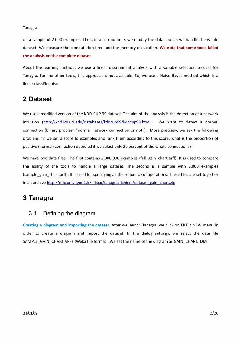
Automatic  feature  selection.  Some  of  the  INPUT  attributes  are  irrelevant  or  redundant. We  insert  the 

STEPDISC  (FEATURE  SELECTION  tab)  component  in  order  to  detect  the  relevant  subset  of  predictive 

variables. Setting the size of the subset is very hard. Statistical cut values are not really useful here because 

we apply the process on a large dataset, all the variables seem significant.  

So,  the  simplest way  is  the  trial  and  error  approach. We  observe  the  decreasing  of  the WILKS  Lambda 

statistic when we add a new predictive variable. The good choice seems SUBSET SIZE = 6. When we add a 

new  variable  after  this  step,  the  decreasing  of  the  Lambda  is  comparatively  weak.  This  corresponds 

approximately  to  the elbow of  the  curve underlining  the  relationship between  the number of predictive 

variable and the Wilks' lambda. We set the settings according to this point of view. 

 

Tanagra 

21/01/09    6/26 

 

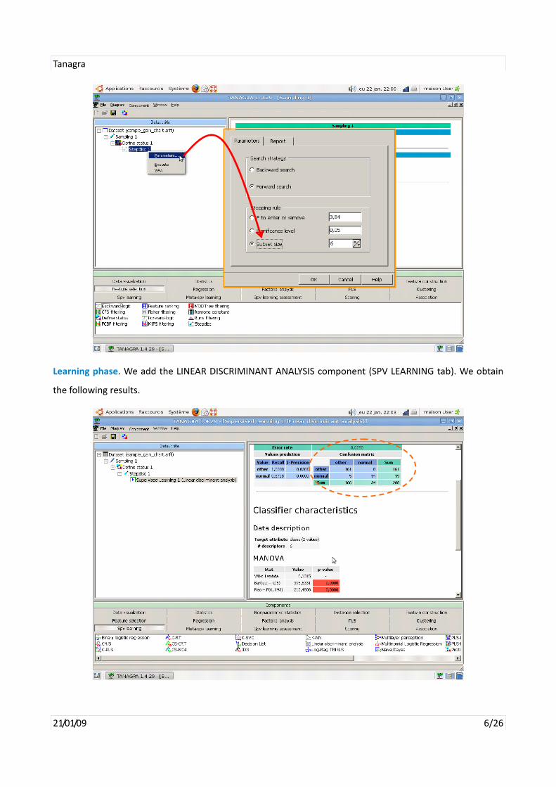
Learning phase. We add the LINEAR DISCRIMINANT ANALYSIS component (SPV LEARNING tab). We obtain 

the following results. 

 

Tanagra 

21/01/09    7/26 

Computing the score column. We compute now the score (the score value is not really a probability, but it 

allows to rank the examples as the conditional probability P[CLASS = positive /  INPUT attributes]) of each 

example to be a positive one. It is computed on the whole dataset i.e. both the train and the test set. 

We add the SCORING component (SCORING tab). We set the following parameters i.e. the "positive" value 

of the class attribute is "normal". A new column SCORE_1 is added to the dataset. 

 

Creating the gain chart. In order to create the GAIN CHART, we must define the TARGET (CLASSE) attribute 

and the SCORE attributes (INPUT). We use the DEFINE STATUS component from the tool bar. We note that 

we  can  set  several  SCORE  columns,  this  option will  be  useful when we want  to  compare  various  score 

columns (e.g. when we want to compare the efficiency of various  learning algorithms which compute the 

score). 

 

Tanagra 

21/01/09    8/26 

 

Then, we add the LIFT CURVE component (SCORING tab). The settings correspond to the computation of the 

curve on the "normal" value of the class attribute, and on the unselected examples i.e. the test set. 

 

Tanagra 

21/01/09    9/26 

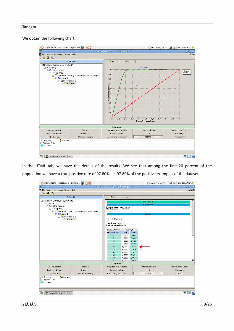
We obtain the following chart. 

 

In  the  HTML  tab,  we  have  the  details  of  the  results. We  see  that  among  the  first  20  percent  of  the 

population we have a true positive rate of 97.80% i.e. 97.80% of the positive examples of the dataset. 

 

Tanagra 

21/01/09    10/26 

3.2 Running the diagram on the complete dataset

This first step allows us to define the sequence of data analysis. Now, we want to apply the same framework 

on the complete dataset. We create the classifier on a learning set with 200,000 instances, and evaluate its 

performance, using a gain chart, on a test set with 1,800,000 examples. 

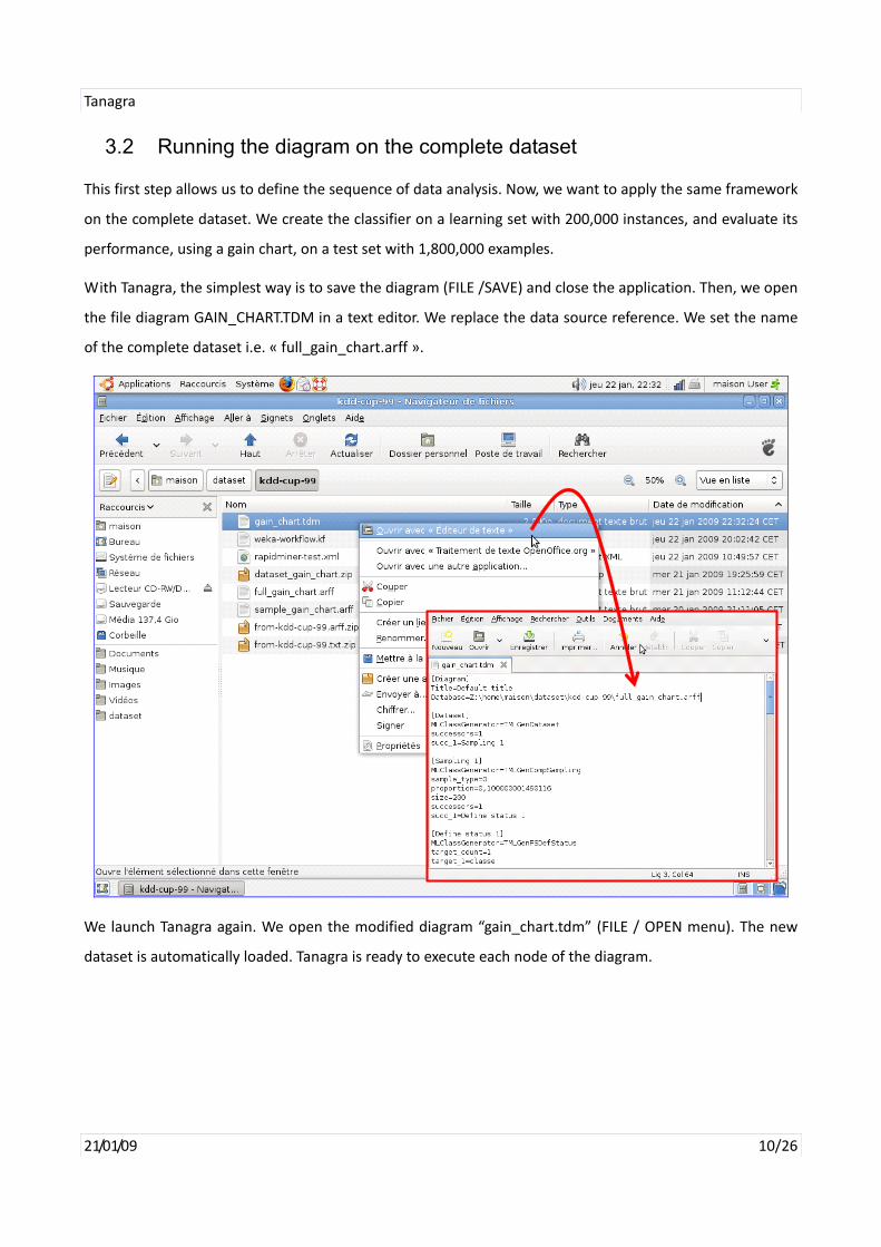
With Tanagra, the simplest way is to save the diagram (FILE /SAVE) and close the application. Then, we open 

the file diagram GAIN_CHART.TDM in a text editor. We replace the data source reference. We set the name 

of the complete dataset i.e. « full_gain_chart.arff ». 

 

We  launch Tanagra again. We open the modified diagram “gain_chart.tdm”  (FILE / OPEN menu). The new 

dataset is automatically loaded. Tanagra is ready to execute each node of the diagram. 

 

Tanagra 

21/01/09    11/26 

 

The processing time is 180 seconds (3 minutes).  

 

Tanagra 

21/01/09    12/26 

We execute all operations with  the DIAGRAM  / EXECUTE menu. We get  the  table associated  to  the gain 

chart. Among the 20% first individuals (according to the score value), we find 98.68% of positives (the true 

positive rate is 98.68%). 

 

Here is the gain chart. 

 

Tanagra 

21/01/09    13/26 

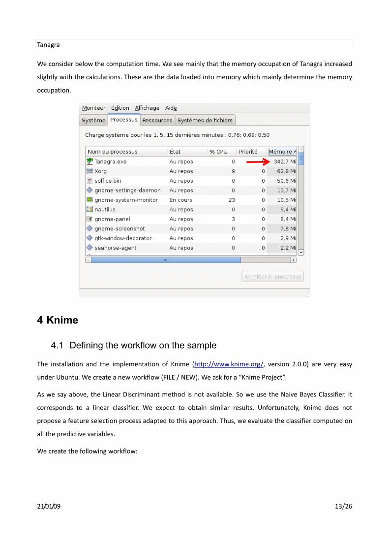
We consider below the computation time. We see mainly that the memory occupation of Tanagra increased 

slightly with the calculations. These are the data loaded into memory which mainly determine the memory 

occupation. 

 

4 Knime

4.1 Defining the workflow on the sample

The  installation  and  the  implementation  of  Knime  (http://www.knime.org/,  version  2.0.0)  are  very  easy 

under Ubuntu. We create a new workflow (FILE / NEW). We ask for a “Knime Project”. 

As we say above, the Linear Discriminant method  is not available. So we use the Naive Bayes Classifier.  It 

corresponds  to  a  linear  classifier.  We  expect  to  obtain  similar  results.  Unfortunately,  Knime  does  not 

propose a feature selection process adapted to this approach. Thus, we evaluate the classifier computed on 

all the predictive variables. 

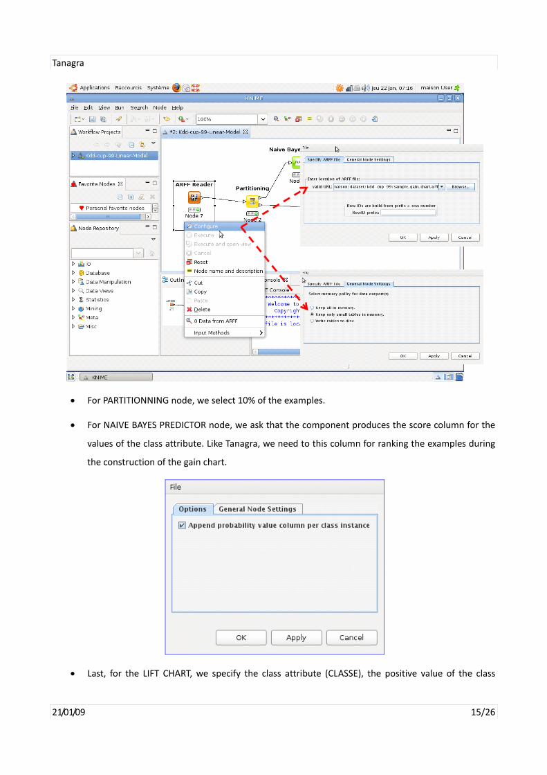
We create the following workflow: 

Tanagra 

21/01/09    14/26 

 

We describe below the settings of some components. 

• ARFF  READER:  The  dialog  box  appears  with  the  CONFIGURE menu. We  set  the  file  name  i.e. 

“sample_gain_chart.arff”. Another very important parameter is in the GENRAL NODE SETTINGS tab. 

If the dataset is too large (higher than 100,000 examples according to the documentation), it can be 

swapped on the disk. It is the only software of this tutorial which does not load the entire data set 

in memory during the processing. In this point of view, it is similar to the commercial tools that can 

handle  very  large  databases.  Certainly,  it  is  an  advantage.  We  see  the  consequences  of  this 

technical choice when we have to handle the complete database. 

 

Tanagra 

21/01/09    15/26 

 

• For PARTITIONNING node, we select 10% of the examples. 

• For NAIVE BAYES PREDICTOR node, we ask that the component produces the score column for the 

values of the class attribute. Like Tanagra, we need to this column for ranking the examples during 

the construction of the gain chart. 

 

• Last,  for  the  LIFT CHART, we  specify  the  class  attribute  (CLASSE),  the positive  value of  the  class 

Tanagra 

21/01/09    16/26 

attribute (NORMAL). The width of the interval (INTERVAL WIDTH) for the construction of the table 

is 10% of the examples. 

 

When we  click  on  the  EXECUTE  AND OPEN  VIEW  contextual menu, we  obtain  the  following  gain  chart 

(CUMULATIVE GAIN CHART tab). 

 

Tanagra 

21/01/09    17/26 

4.2 Calculations on the complete database

We are ready to work on the complete base. We activate again the dialog settings of the ARFF READER node 

(CONFIGURE menu). We  select  the  « full_gain_chart.arff »  data  file. We  can  execute  the workflow. We 

obtain the following gain chart. 

 

The results are very similar to those obtained on the sample (2,000 examples).  

The computation time however is not really the same. It is very high compared to that of Tanagra. We study 

in details below the computation time of each step. 

About the memory occupation, the system monitor shows that Knime uses "only" 193 Mo (Figure 1).  It  is 

clearly lower than Tanagra; it will be lower than all other tools we analyze in this tutorial. 

We can clearly see the advantages and disadvantages of swapping data on the disk: the memory  is under 

control, but  the  computation  time  increases.  If we are  in  the phase of  final production of  the predictive 

model,  it  is not a problem.  If we are  in  the exploratory phase, where we use  trial and error  in order  to 

define the best strategy, prohibitive computation time is discouraging. 

In this configuration, the only solution is to work on sample. In our study, we note that the results obtained 

Tanagra 

21/01/09    18/26 

on 2,000 cases are very close  to  the  results obtained on 2,000,000 examples. Of course,  it  is an unusual 

situation. The underlying concept between  the class attribute and  the predictive attribute  is very simple. 

But, it is obvious that, if we can determine the sufficient sample size for the problem, this strategy allows us 

to explore deeply the various solutions without a prohibitive calculations time. 

 

Figure 1 – Memory occupation of Knime during the processing 

5 RapidMiner

The  installation  and  the  implementation  of  RapidMiner  (http://rapid‐i.com/content/blogcategory/38/69/, 

Community Edition, version 4.3) are very simple under Ubuntu. We add on  the desktop a shortcut which 

runs automatically the Java Virtual Machine with “rapidminer.jar” file. 

5.1 Working on the sample

As  the  other  tools, we  set  the  sequence  of  operations  on  the  sample  (2,000  examples).  There  is  little 

documentation on the software. However, it comes with many predefined examples. We often find quickly 

an example of analysis which is similar to ours. 

About  the gain chart, we get  the example  file « sample/06_Visualization/16_LiftChar.xlm ». We adapt  the 

Tanagra 

21/01/09    19/26 

sequence of operations on our dataset. 

 

I do not really understand all. The operators IORetriever and IOStorer seem quite mysterious. Anyway, the 

important thing is that RapidMiner provides the desired results. And it is. 

 

Tanagra 

21/01/09    20/26 

 

We see into this chart: there are 1,800 examples into the test set; there are 324 positive examples (CLASSE 

= NORMAL). Among the first 20% of the dataset (360 examples) ranked according to the score value, there 

are 298 positive examples i.e. the true positive rate is 298 / 324 # 92%. 

We use the following settings for this analysis: 

• SIMPLEVALIDATION : SPLIT_RATIO = 0.1 ; 

• LIFT PARETO CHART : NUMBER OF BINS = 10 

We use the Naive Bayes classifier for Rapidminer because the linear discriminant analysis is not available. 

 

Tanagra 

21/01/09    21/26 

5.2 Calculations on the complete database

To  run  the  calculations  on  the  complete  database, we modify  the  settings  of  ARFF  EXAMPLE  SOURCE 

component. Then, we click on the PLAY button into the tool bar. 

 

 

 

The calculation was failed. The base was  loaded  in 17 minutes; the memory  is  increased to 700 MB when 

the crash occurred. The message sent by the system is the following 

 

Tanagra 

21/01/09    22/26 

 

6 Weka

Weka is a well‐known machine learning software (http://www.cs.waikato.ac.nz/ml/weka/, Version 3‐6‐0). It 

runs under a JRE (Java Runtime). The installation and the implementation are easy.  

There  are  various ways  to use Weka. We  choose  the KNOWLEDGEFLOW mode  in  this  tutorial.  It  is  very 

similar to Knime. 

6.1 Working on the sample

As  the  other  tools,  we  work  on  the  sample  in  a  first  time  in  order  to  define  the  entire  sequence  of 

operations.   

We  see below  the diagram. We  voluntarily  separate  the  components. Thus we  see,  in blue,  the  type of 

information  transmitted  from  an  icon  to  another.  It  is  very  important.  It  determines  the  behavior  of 

components. 

 

Tanagra 

21/01/09    23/26 

 

We describe here some nodes and settings:  

• ARFF LOADER loads the data file « sample_gain_chart.arff »; 

• CLASS ASSIGNER specifies the class attribute « classe », all the other variables are the descriptors; 

• CLASS VALUE PICKER defines the positive value of the class attribute i.e. « CLASSE = NORMAL »; 

• TRAIN TEST SPLIT MAKER splits the dataset, we select 10% for the train set; 

• NAIVE BAYES  is  the  learning method, we connect  to  this component both  the TRAINING SET and  the 

TEST SET connections; 

• CLASSIFIER PERFORMANCE EVALUATOR evaluates the classifier performance; 

• MODEL PERFORMANCE CHART creates various charts for the classifier evaluation on the test set. 

To start the calculations, we click on the START LOADING menu of the ARFF LOADER component. The results 

are available by clicking on the SHOW CHART menu of the MODEL PERFORMANCE CHART component. 

Weka offers  a  clever  tool  for  visualizing  charts. We  can  select  interactively  the  x‐coordinates  and  the  y‐

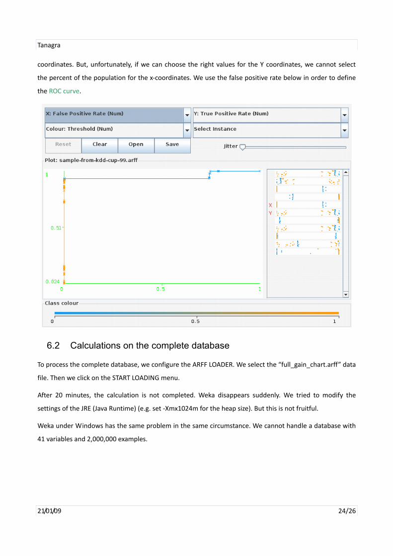
Tanagra 

21/01/09    24/26 

coordinates. But, unfortunately,  if we can choose the right values  for the Y coordinates, we cannot select 

the percent of the population for the x‐coordinates. We use the false positive rate below in order to define 

the ROC curve. 

 

6.2 Calculations on the complete database

To process the complete database, we configure the ARFF LOADER. We select the “full_gain_chart.arff” data 

file. Then we click on the START LOADING menu. 

After  20 minutes,  the  calculation  is  not  completed. Weka  disappears  suddenly. We  tried  to modify  the 

settings of the JRE (Java Runtime) (e.g. set ‐Xmx1024m for the heap size). But this is not fruitful. 

Weka under Windows has the same problem in the same circumstance. We cannot handle a database with 

41 variables and 2,000,000 examples. 

 

Tanagra 

21/01/09    25/26 

7 Conclusion

Of course, maybe I have not set the optimal settings for the various tools. But they are free, the dataset is 

available on  line, anyone can make the same experiments, and try other settings  in order to  increase the 

efficiency  of  the  processing,  both  about  the  computation  time  and  the  memory  occupation  (e.g.  the 

settings of the JRE – Java Runtime Environment). 

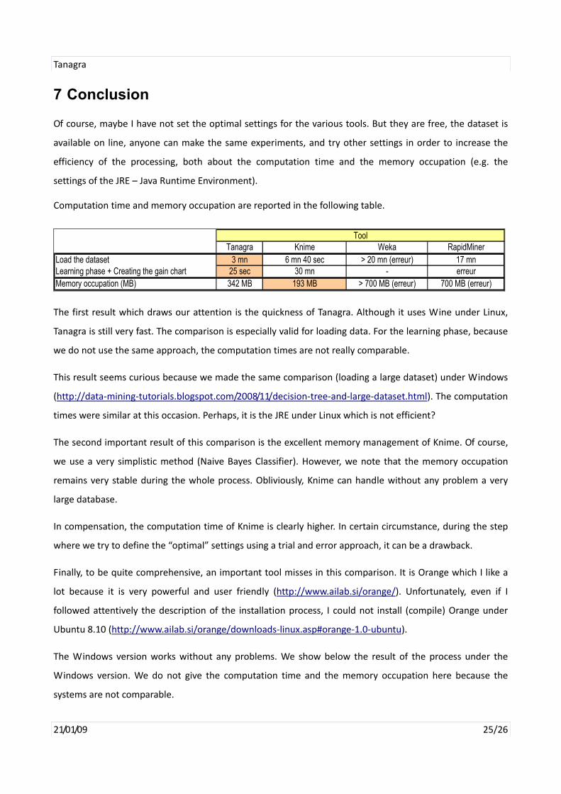
Computation time and memory occupation are reported in the following table. 

Tanagra Knime Weka RapidMinerLoad the dataset 3 mn 6 mn 40 sec > 20 mn (erreur) 17 mnLearning phase + Creating the gain chart 25 sec 30 mn - erreurMemory occupation (MB) 342 MB 193 MB > 700 MB (erreur) 700 MB (erreur)

Tool

 

The first result which draws our attention  is the quickness of Tanagra. Although  it uses Wine under Linux, 

Tanagra is still very fast. The comparison is especially valid for loading data. For the learning phase, because 

we do not use the same approach, the computation times are not really comparable. 

This result seems curious because we made the same comparison (loading a large dataset) under Windows 

(http://data‐mining‐tutorials.blogspot.com/2008/11/decision‐tree‐and‐large‐dataset.html). The computation 

times were similar at this occasion. Perhaps, it is the JRE under Linux which is not efficient? 

The second important result of this comparison is the excellent memory management of Knime. Of course, 

we use a very simplistic method  (Naive Bayes Classifier). However, we note  that  the memory occupation 

remains very stable during  the whole process. Obliviously, Knime can handle without any problem a very 

large database.  

In compensation, the computation time of Knime is clearly higher. In certain circumstance, during the step 

where we try to define the “optimal” settings using a trial and error approach, it can be a drawback. 

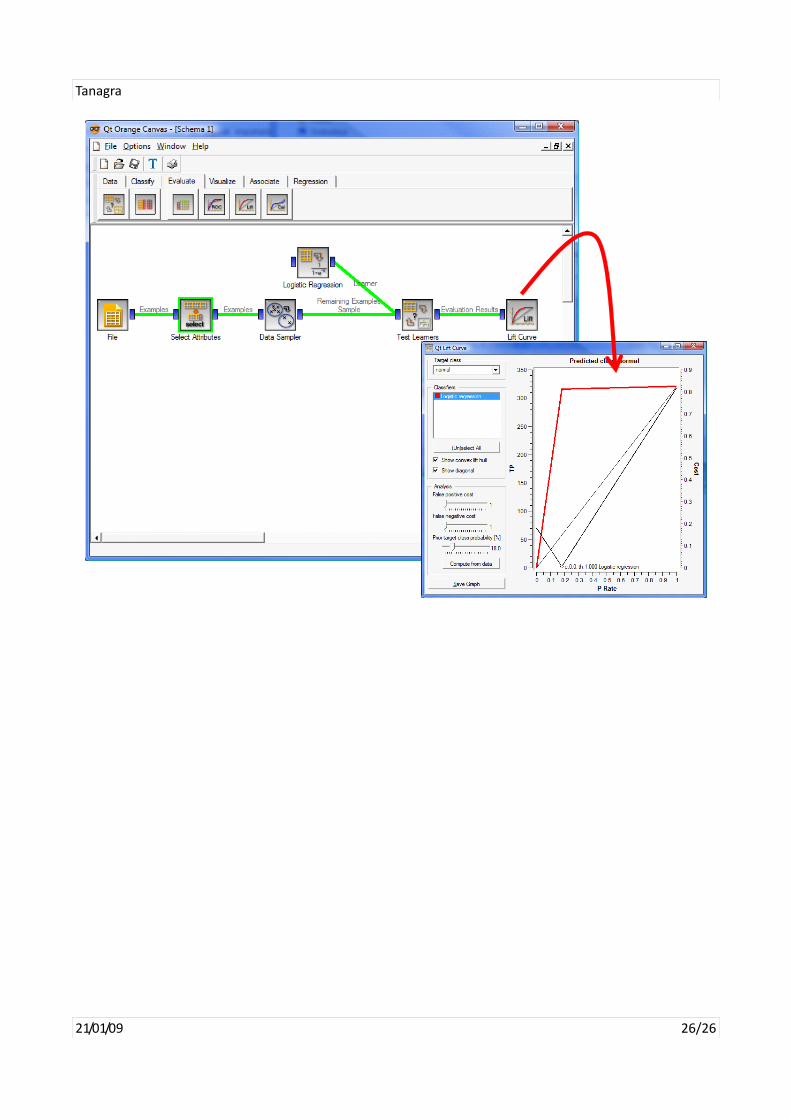
Finally, to be quite comprehensive, an important tool misses in this comparison. It  is Orange which I like a 

lot  because  it  is  very  powerful  and  user  friendly  (http://www.ailab.si/orange/).  Unfortunately,  even  if  I 

followed attentively  the description of  the  installation process,  I could not  install  (compile) Orange under 

Ubuntu 8.10 (http://www.ailab.si/orange/downloads‐linux.asp#orange‐1.0‐ubuntu). 

The Windows version works without any problems. We  show below  the  result of  the process under  the 

Windows  version. We do not  give  the  computation  time  and  the memory occupation here because  the 

systems are not comparable. 

Tanagra 

21/01/09    26/26