Embed Size (px)
Citation preview

1
Gross Domestic Product (GDP) which gauges the total production
of all final goods and services produced in an economy during a
period of time. Empirically, for most of the countries, particularly
for those advanced countries, GDP demonstrates an upward
trend in the long run. However, in the short run, we observe that
GDP fluctuates around this long term trend. During economic
booms, consumption increases and firms invest more, GDP goes
up. During recessions, consumers spend less and firms cut its
investment, GDP goes down. The ups and downs of GDP not only
affect the living standards, but also employment levels.
2

Aggregate demand (AD) and aggregate
supply (AS) model was developed to analyze
the determination of output and price levels.
We will then illustrate how changes in AD
and AS affect the output and price levels.
After that, we will discuss the relationship
between output and employment levels.
3
2.1 What is aggregate demand?
◦ GDP (Y) is made up of four components: consumption
(C), investment (I), government purchases (G), and net
exports (NX). Each of the four components is a part of
aggregate demand (AD). Then we have:
◦ Y = C + I + G + NX
4

The AD curve shows the relationship
between price and the quantity of output
(real GDP) demanded by the households,
firms and the government.
5

A downward sloping AD curve indicates that a fall in
the price level increases the demand for real GDP,
and vice versa. This means that to understand why
the aggregate-demand curve slopes downward, we
must understand how changes in the price level
affect consumption, investment, and net exports.
Government purchases are assumed to be fixed by
policy, not by price level. G is thus not included in
the analysis at this stage.
6

Figure 1 A Downward-Sloping Aggregate-Demand Curve
7
The Wealth Effect: The Price Level and
Consumption:
◦ A household’s wealth is the difference between the value of its
assets and the value of its debt. For example, if you hold all
your $10,000 assets in cash and you have no debt, your wealth
is $10,000. Suppose that the price level unexpectedly drops by
20%, the real value of your wealth will increase by 20% as your
purchasing power has increased. A decrease in the price level
makes consumers become wealthier, which in turn encourages
them to spend more. The increase in consumer spending means
a larger quantity of goods and services demanded.
8
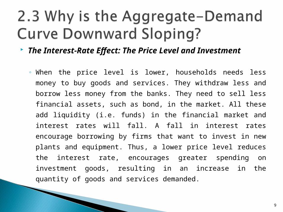
The Interest-Rate Effect: The Price Level and Investment
◦ When the price level is lower, households needs less money to
buy goods and services. They withdraw less and borrow less
money from the banks. They need to sell less financial assets,
such as bond, in the market. All these add liquidity (i.e. funds)
in the financial market and interest rates will fall. A fall in
interest rates encourage borrowing by firms that want to invest
in new plants and equipment. Thus, a lower price level reduces
the interest rate, encourages greater spending on investment
goods, resulting in an increase in the quantity of goods and
services demanded.
9
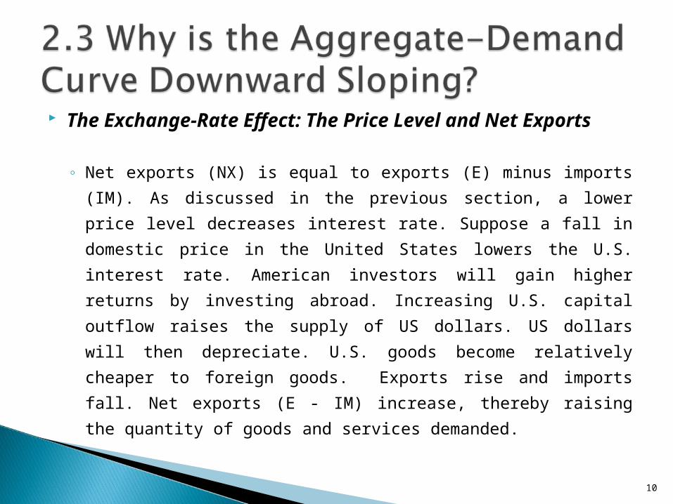
The Exchange-Rate Effect: The Price Level and Net Exports
◦ Net exports (NX) is equal to exports (E) minus imports (IM). As
discussed in the previous section, a lower price level decreases
interest rate. Suppose a fall in domestic price in the United
States lowers the U.S. interest rate. American investors will gain
higher returns by investing abroad. Increasing U.S. capital
outflow raises the supply of US dollars. US dollars will then
depreciate. U.S. goods become relatively cheaper to foreign
goods. Exports rise and imports fall. Net exports (E - IM)
increase, thereby raising the quantity of goods and services
demanded.
10

Don’t Confuse!
◦ Shift of the AD curve versus Movement along the AD curve The AD curve shows the relationship between price level and output
demanded, holding all other factors unchanged. As discussed
above, when price changes, the output level changes due to the
wealth effect, interest-rate effect and exchange-rate effect. The
economy will move up or down along the AD curve. However, when
other factors, such as government policy, change, prices remain
unchanged, the whole AD curve will shift to the right or left. For
example, when government increases spending on infrastructure, the
AD curve will shift to the right. This shift is caused by government
policy, not by the changes in price levels.
11

Don’t Confuse!◦ Shift of the AD curve versus Movement
along the AD curve Figure 2 Shift of the AD Curve
12

As mentioned above, when price keeps constant,
other factors may change aggregate demand,
which shifts the AD curve to the left or right.
These ‘other factors’ are called the determinants
of aggregate demand. Put it in another way,
these determinants are the factors shifting the
AD curve while keeping prices unchanged. The
factors are discussed below.
13

Private consumption expenditure
◦ Other things being equal, an increase in private
consumption expenditure will shift the AD curve
to the right and vice versa. Private consumption
expenditure are mainly determined by:
14

Private consumption expenditure
◦ Disposable income (after-tax income): If the
government cuts taxes, it encourages people to spend
more, resulting in an increase in aggregate demand.
◦ Desire to save: If Hong Kong people become more
concerned with saving for retirement and reduce
current consumption, aggregate demand will decline.
15

Private consumption expenditure
◦ Wealth (value of assets): If the Hong Kong
stock market booms, people become wealthier
and they tend to spend more.
◦ Interest rate: When interest rate falls, people
find the costs of borrowing lower and they have
higher incentive to borrow for consumption.
16

Investment expenditure
◦ Any factors fostering firms to invest more shift the
AD curve to the right and vice versa. Firms’
incentives to invest are determined primarily by:
17

Investment expenditure ◦ Productivity of factor inputs: If a firm finds new tools
and machinery (e.g. a faster computer) that can increase
output given the same resources, firms are more willing
to invest in the new tools and machinery.
◦ Business prospects: Optimistic business prospects
offers better returns on investment. Business firms have
higher incentive to invest. Pessimistic business
conditions incentivize firms to cut back investment
spending.
18

Investment expenditure
◦ Government policy: Government policy can
encourage or discourage investment. For example, tax
exemption for investment will motivate firms to invest
more.
◦ Money supply and interest rate: An increase in the
supply of money lowers the interest rate in the short
run. This lead to more investment spending, which
causes an increase in aggregate demand.
19

Government expenditure
◦ When government increases expenditure on
infrastructure or other services such as education
and medical services, it shifts the AD curve to the
right and vice versa for a decrease in government
expenditure.
20

Net export
◦ Net exports (NX) equals exports minus imports, which is mainly
determined by the economic conditions of trading partners and
exchange rate.
◦ Economic conditions of foreign countries: When the income levels of
foreign countries (i.e. trading partners) grow faster than that of
domestic economy, foreign countries will buy more goods from the
domestic economy and NX of domestic economy will rise. The AD curve
will shift to the right. On the contrary, if the income level of domestic
economy grows faster than those of foreign countries, domestic
economy will import more and export less. NX will fall and the AD curve
will shift to the left.
21

Net export
◦ Exchange rate: NX will fall when the value of domestic currency
rises against foreign currency. To illustrate, if the exchange rate
between euro and US$ changes from €1 = US$1.5 to €1 =
US$1.7, the value of euro increases and the prices of European
products in the US will rise, which makes European goods less
competitive in the US market. The NX of European countries will
fall and the AD curve will shift to the left. By the same analysis,
a decrease in value of domestic currency will make domestically
produced goods more competitive in the overseas market. It will
shift the AD curve to the right.
22
Don’t Confuse!
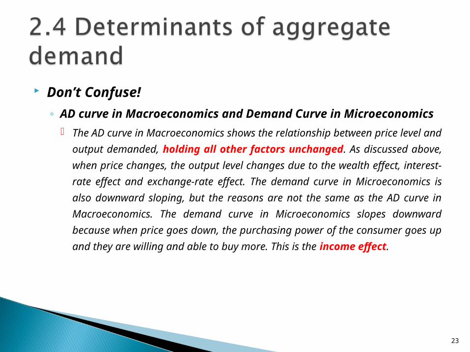
◦ AD curve in Macroeconomics and Demand Curve in
Microeconomics The AD curve in Macroeconomics shows the relationship between
price level and output demanded, holding all other factors
unchanged. As discussed above, when price changes, the output
level changes due to the wealth effect, interest-rate effect and
exchange-rate effect. The demand curve in Microeconomics is also
downward sloping, but the reasons are not the same as the AD curve
in Macroeconomics. The demand curve in Microeconomics slopes
downward because when price goes down, the purchasing power of
the consumer goes up and they are willing and able to buy more. This
is the income effect.
23

Don’t Confuse!
◦ AD curve in Macroeconomics and Demand Curve in
Microeconomics
At the same time, the fall in price of the goods makes the good relatively
cheaper and more attractive, given prices of other good remain unchanged.
The consumer will buy more the cheaper good. This is the substitution
effect. Demand curve in Microeconomics is for a single product, so we can
have substitution effect. However, the AD curve in Macroeconomics depicts
the relationship of general price level and aggregate output level (i.e. all
goods and service produced). A rise in general price level means that the
prices of all domestically produced goods and services are rising. Consumers
have no other goods and services which they can substitute for. There is no
substitution effect for AD curve in Macroeconomics.
24

3.1 What is aggregate supply?
◦ Aggregate supply (AS) refers to the total amount
of goods and services supplied by the firms in an
economy.
25

The aggregate supply (AS) curve shows the relationship
between price and the quantity of output that firms are
willing and able to supply.
It must be noted that since the effects of changes in
price level on aggregate supply is very different in short
run and long run, we will use two AS curves, the short-
run aggregate-supply (SRAS) curve and the long-run AS
curve, for our analysis. We will first examine the long-run
aggregate-supply (LRAS) curve.
26

In the long run, an economy’s production of goods and services
depends on its supplies of resources (labour, capital and natural
resources) along with the available production technology. In other
words, we can say that our long run production capacity is
constrained by the available resources and technology. Then we can
further infer that price will have no effects on output level in the long
run because price increase or decrease will not change the amount of
resources and technology available in the economy. Because the price
level does not affect the determinants of output in the long run, the
long-run aggregate-supply curve is vertical.
27

Figure 3 Long-Run Aggregate-Supply (LRAS) Curve
28

The position of the LRAS occurs at an output level
sometimes referred to as potential output or full-
employment output. This is the level of output that the
economy produces when resources are fully utilised (i.e.
firms produce at their full capacity) and unemployment
is at its natural rate (i.e. full employment level). The full
employment level refers to the employment level that all
people who want to find a job will have one, except
those structurally and frictionally unemployed.
29

Knowledge Recap◦ Structural and frictional unemployment:
Structural unemployment refers to the
unemployment caused by the mismatch of the skills
and attributes of workers and the requirements of
the jobs. Frictional unemployment refers to the
short-term unemployment arising from the time and
process of matching job-seekers and the jobs
available.
30

Based on the above discussion, it follows that
any factors, which can change the natural rate
of output, will shift the long-run aggregate-
supply curve. There are four factors which are
able to change the production capacity of an
economy, which in turn shifts the LRAS. The
factors are examined as follows:
31

Labour: Labour supply can be increased by growth in population,
increases in immigrants, and a fall in the natural rate of
unemployment. The long-run aggregate-supply curve would shift to
the right.
Capital: Capital includes both physical and human capital. An
increase in the economy’s physical capital stock (e.g. factories,
machinery, tools, etc.) raises productivity and thus shifts the LRAS to
the right. The rightward shift of LRAS curve can also be accomplished
by an increase in human capital (e.g. skills and knowledge of the
workers).
32

Natural Resources: A discovery of a new minerals and natural
resources increases long-run aggregate supply. On the contrary, a
change in weather patterns (more frequent drought and floods) that
makes farming more difficult shifts long-run aggregate supply to the left.
Technological Knowledge: Technological change refers to an advance
in knowledge which improves ways to produce goods and services, that
is to improve the production efficiency of goods and services. The
invention of the computer has allowed us to produce more goods and
services from any given level of resources. As a result, it has shifted the
long-run aggregate-supply curve to the right.
33

The LRAS is vertical because prices have no effect on
output in the long run. However, the SRAS curve is
upward sloping, which indicates that an increase in the
overall price level tends to raises the quantity of goods
and services supplied and a decrease in the overall price
level tends to lower the quantity of goods and services
supplied in the economy.
Why is there a positive relationship between price and
output levels in the short run? There are three theories
put forward to explain this relationship.
34

Figure 4 Short-Run Aggregate-Supply (SRAS) Curve
35
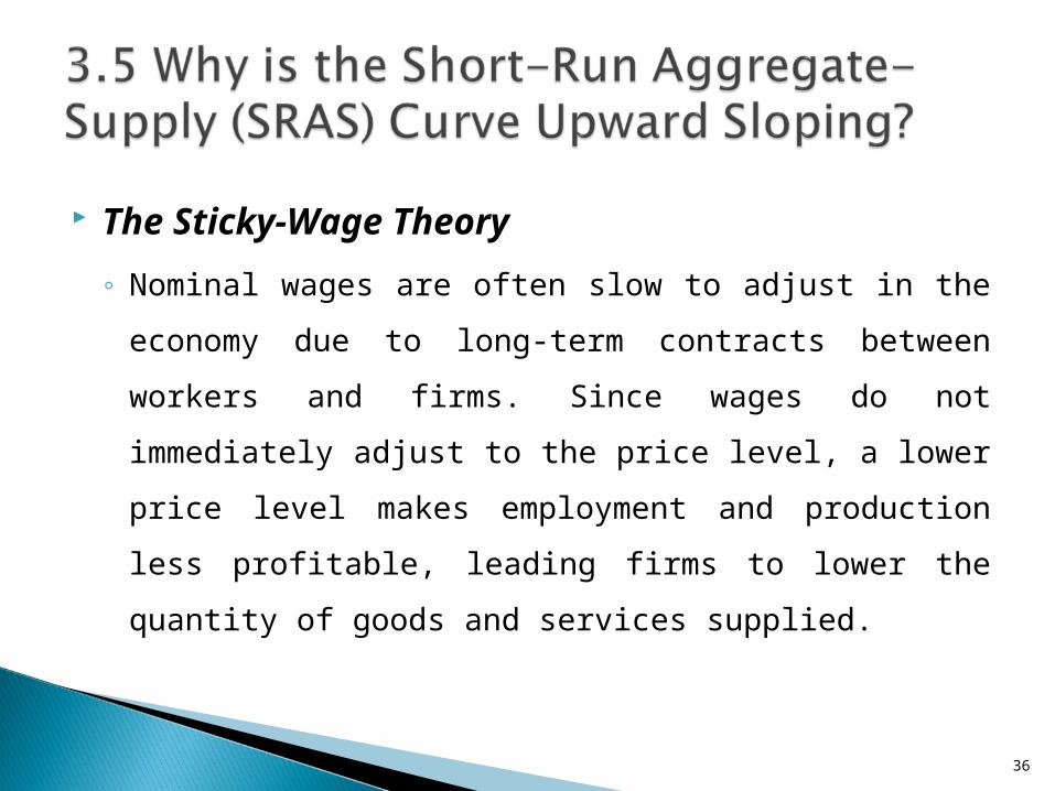
The Sticky-Wage Theory
◦ Nominal wages are often slow to adjust in the
economy due to long-term contracts between
workers and firms. Since wages do not
immediately adjust to the price level, a lower
price level makes employment and production
less profitable, leading firms to lower the quantity
of goods and services supplied.
36

The Sticky-Wage Theory
◦ For instance, suppose a firm has agreed in
advance to pay workers a certain amount and then
the price level falls unexpectedly. This implies that
the firm is now paying a real wage (wage/price)
that is larger than it intended. It raises the costs of
production. Thus, the firm hires less labor and
produces a smaller quantity of goods and services.
37

The Sticky-Price Theory
◦ The prices of some goods and services are also sometimes slow
to respond to changes in the economy because of the costs of
adjusting prices which is named as menu costs. Menu costs
include the costs of printing new menu and catalog as well as
the time involved. If the price level falls unexpectedly, some
firms immediately adjust their prices downward, but there are
firms which do not change the price of its products quickly. It
may be due to the fact that these firms would like to
temporarily avoid the menu costs. Their relative price will rise
and this will lead to a loss in sales.
38

The Sticky-Price Theory
◦ Thus, when sales decline, firms will produce a
lower quantity of goods and services. In a word,
because not all prices adjust instantly to changing
conditions, an unexpected fall in the price level
leaves some firms with higher-than-desired
prices, which depresses sales and causes firms to
lower the quantity of goods and services supplied.
39
The Misperceptions Theory
Changes in the overall price level can
temporarily mislead suppliers about what is
happening in the markets in which they sell
their output. As a result of these
misperceptions, suppliers respond to changes
in the level of prices which causes the short-run
aggregate-supply curve to be upward sloping.
40

The Misperceptions Theory
To explain the theory in a more concrete way, suppose that the
general price level falls unexpectedly. Some firms mistakenly believe
that the price of their products falls and they perceive it as a fall in the
relative price of their products. Firms may then believe that the
reward of supplying their product has fallen, and thus they decrease
the quantity that they supply. Thus, a lower general price level causes
misperceptions about relative prices, and these misperceptions lead
firms to respond to the lower price level by decreasing the quantity of
goods and services supplied.
41

Don’t Confuse!
◦ The Sticky-Price Theory and the Misperceptions
Theory
Please note that the Sticky-Price Theory explains that
because some suppliers are slow to response to general
price level and that is why SRAS is upward sloping while the
Misconceptions Theory explains that the SRAS curve is
upward sloping because some suppliers over-respond to
general price level. This over-response may be due to the
lack of information facing the firms.
42
Factors that shift the long-run aggregate-
supply curve will also shift the short-run
aggregate-supply curve. However, people’s
expectations of the price level will affect the
position of the short-run aggregate-supply
curve even though it has no effect on the
long-run aggregate-supply curve.
43

A higher expected price level decreases the quantity of
goods and services supplied and shifts the short-run
aggregate-supply curve to the left. Suppose workers and
firms expect the future price will increase by 5 percent,
workers or unions will negotiate a rise in wage by 5
percent to maintain their purchasing power. If all firms
and workers expect in the same way, the costs of
production will increase by 5 percent and the SRAS
curve will shift to the left.
44

By the same analysis, a lower expected
price level increases the quantity of goods
and services supplied and shifts the short-
run aggregate-supply curve to the right.
45

In the short run, not all prices, including prices of factor inputs (e.g.
wages), adjust at the same pace. Therefore, when price level goes up,
firms are willing to supply more goods and services because profits
are higher. As a result, the SRAS curve is upward-sloping. However, in
the long run, all prices, including prices of factor inputs, are fully (or
completely) adjusted. The 3 percent change in price level will be
accompanied by 3 percent change in factor prices. Any increase in
profits are absorbed by the rise of input prices, so the firm will have
no incentive to increase the supply of goods and services. It follows
that change in price level will have no effect on aggregate supply in
the long run. The LRAS curve is thus vertical.
46

4.1 Determinants of equilibrium output
and price levels in the long run◦ Long-run equilibrium is found where the aggregate-
demand curve intersects with the long-run aggregate-
supply curve. Output is at its natural rate. Also at this
point, perceptions, wages, and prices have fully
adjusted and resources are utilized at its capacity.
Therefore, the short-run aggregate-supply curve and
aggregate-demand curve intersects at the potential
(i.e. full employment) output level.
47

4.1 Determinants of equilibrium output and price levels in the long run◦ Figure 5 Long Run Equilibrium
48
Any changes in AD and AS will result in
changes in price and output levels in the
short run. However, the automatic
adjustment mechanism in the market can
restore the economy back to long-run
equilibrium. We will start our analysis with
the change in AD.
49

The effects of a shift in aggregate demand◦ Figure 6 The Effects of a Shift in AD
50

The effects of a shift in aggregate demand
◦ Suppose households and firms are pessimistic about
the future economic conditions, which causes
households’ spending and firms’ investment to decline.
This shifts the aggregate demand curve to shift to the
left. In the short run, the equilibrium moves from A to
B. Both output and the price level fall. This drop in
output means that the economy is in a recession.
51

The effects of a shift in aggregate
demand
◦ It is not uncommon for the government to
eliminate the recession by boosting government
spending. By doing so, aggregate demand curve
shifts back to the right. The equilibrium moves
back from B to A.
52

The effects of a shift in aggregate demand
◦ However, even if the government does nothing, it is possible that the
economy will eventually move back to the natural rate of output. As
shown in Figure 6, under recession, price falls from P1 to P2. Workers and
firms are willing to adjust their sticky wages and sticky prices. When
output is low, unemployment is high. Workers are now willing to accept
lower wages and firms are willing to accept lower prices. After all
adjustments, the aggregate-supply curve shifts to the right, from SRAS1
to SRAS2. Equilibrium moves from B to C, reaching again the natural
rate of output at a lower price level P3. The process of adjustment back
to the natural rate of output is called the automatic adjustment
mechanism.
53

The effects of a shift in aggregate
demand
◦ In the long run, the decrease in aggregate
demand causes a drop in the equilibrium price
level, but leave the output level unchanged. Thus,
the long-run effect of a change in aggregate
demand is a nominal change (in the price level)
but not a real change (output is the same).
54
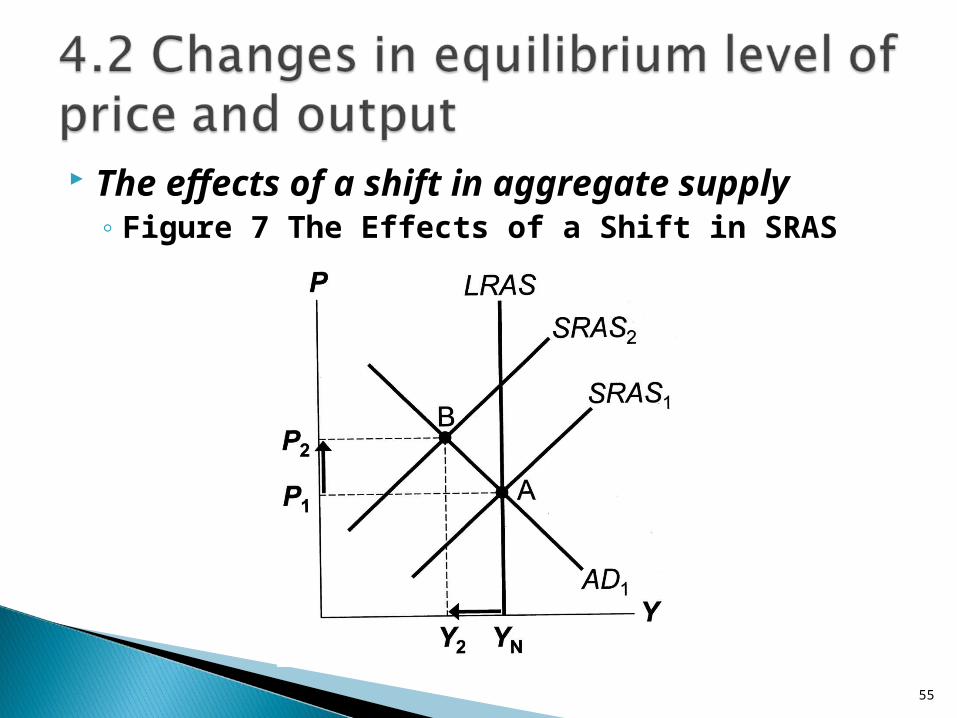
The effects of a shift in aggregate supply◦ Figure 7 The Effects of a Shift in SRAS
55
The effects of a shift in aggregate supply
◦ Suppose firms face a sudden increase in their costs of
production. This will cause the short-run aggregate-
supply curve to shift to the left. (Assume that it does
not shift the LRAS.) In the short run, output will fall and
the price level will rise, which is called stagflation
(i.e. a period of falling output and rising prices). The
equilibrium moves from A to B.
56
The effects of a shift in aggregate supply◦ If the government does nothing, price and wage
expectations will adjust. With increased
unemployment caused by recession, workers are will
to accept lower wages. When nominal wages fall,
producing goods and services become more profitable
and firms are able and willing to supply more, causing
the short-run aggregate-supply curve to shift back to
the right. Recession gradually ends and employment
rebounds. The equilibrium moves back from B to A.
57
The effects of a shift in aggregate supply
◦ However, if the government is impatient to wait for the
automatic adjustment mechanism (the impatience of the
government may be due to political pressure), it can
shift the aggregate-demand curve by increasing
government expenditure. AD curve shift from AD1 to
AD2. The recession will end, but the price level will be
permanently higher at P3. The higher price level is
pushed by the government’s accommodating policy. The
equilibrium moves from A to B, and then finally to C.
58

The effects of a shift in aggregate supply◦ Figure 8 Accommodating an Adverse Shift in
SRAS
59

The effects of a shift in aggregate supply
◦ It is not difficult to use the AS-AD model to analyze
changes in price and output levels in the short run if
students are able to follow the four steps: Determine whether the event shifts AD or AS curve.
Determine whether the curve concerned shifts to the left or
right.
Use AD-AS diagram to see how the shift changes output and
price in the short run.
Use AD-AS diagram to see how economy moves from the new
short run equilibrium to the new long run equilibrium.
60

5.1 Some Highlights
◦ Forecast GDP growth is 1–3%.
◦ Headline inflation rate (including prices of food and energy) is estimated at 3.5%.
◦ Government expenditure is estimated to reach $393.7 billion for 2012–13, an
increase of 7% compared with the revised estimate for 2011–12; total government
revenue will be $390.3 billion.
◦ Major policy areas include supporting enterprises, preserving employment,
increasing land supply, education, medical and health services, social welfare,
relief measures, promoting development of industries, and infrastructure
development.
◦ Please refer to http://www.budget.gov.hk/2012/eng/highlights.html for further
details.
61

In terms of the impacts on the AS and AD, the
expenditure items can be subdivided into three
categories:
◦ The first category includes the expenditure items having
less prominent effects on both AS and AD as the
amount of expenditure is relatively limited. The
expenditures on supporting enterprises (except the SME
Financing Guarantee Scheme) and preserving
employment fall on this category. The have relatively
slight impact on AD.
62

In terms of the impacts on the AS and AD, the expenditure
items can be subdivided into three categories:
◦ The second category of expenditure items will have more significant
effects on price and output in the short run, but less in the long
run. The social welfare and relief measure belong to this category.
These expenditure items are more substantial and consumptive in
nature, which means that they increase the AD in the short run, but not
much effects on the long run. These policies shift the AD curve to the
right, both price and output level will rise in the short run. Since the
expenditures do not change the available factor inputs and the
production capacity is not much affected, there will be limited effects on
LRAS.
63

In terms of the impacts on the AS and AD,
the expenditure items can be subdivided
into three categories:
◦ The third category includes expenditures having
more significant effects on price and output
in both the short run and the long run.
Education and increase in land supply are two
major policies under this category.
64

Take education as an example. Suppose the
output level is below the full employment
output level. If the original equilibrium is at
A, increase in education expenditure shifts
AD1 to AD. The new equilibrium is at B and
the economy reaches its full employment
level of output.
65

Figure 9 The Impact of Education Expenditure on AS and AD
66

However, if the original equilibrium has already been
at the full employment level (Point B), the increase in
education expenditure will shift AD to AD2. Output
increases from Yf to Y2. Prices go up to P2 and
workers will bargain for higher wage to maintain
their purchasing power. SRAS will shift to the left and
reach the equilibrium point D, resulting in even
higher price level, but restoring the output level back
to Yf.
67

Neverthelesss, education will increase human
capital which increases production capacity of the
economy. The LRAS will shift to the right. If long run
output can be increased to Y2, price level will fall
back to P2. Here, we draw an important conclusion:
any rightward shift in AD will push up prices in the
short run, but the extent of price increase will be
smaller if output level can be increased in the long
run (i.e. a rightward shift of LRAS). (See Figure 10)
68

Figure 10 can also be used to illustrate the case of
increasing land supply. Land supply increases
expand the production capacity of the economy.
LRAS curve shift from LRAS2013 to LRAS2015. Prices
will fall substantially if AD remains unchanged at
AD2013. However, AD is not constant and it increases
over time. Though price level goes up, the extent is
smaller than that under fixed long run output level.
69

Figure 10 The Impact of Increase in Land Supply on AS and AD
70

As a final reminder, it may be helpful for students if they can stick to the four steps to analysing the changes in price and output levels.
71

Hubbard, R. G. and O’Brien, A. P. (2010) Economics, 3rd edition, Pearson, Chapter 24.
Mankiw, N. G. (2012), Principles of Economics, 6th edition, South-Western, CENGAGE Learning, Chapter 33.
O’Sullivan, A., Sheffrin, S. M. and Perez, S. J. (2008) Economics: Principles, Applications and Tools, 5th edition, Pearson, Chapter 9.
72

73