1 Direct sampling method to perform multipleâ€point 2 geostatistical

1 Direct sampling method to perform multiple‐point2 geostatistical simulations

3 Gregoire Mariethoz,1,2 Philippe Renard,1 and Julien Straubhaar1

4 Received 9 December 2008; revised 13 July 2010; accepted 6 August 2010; published XX Month 2010.

5 [1] Multiple‐point geostatistics is a general statistical framework to model spatial6 fields displaying a wide range of complex structures. In particular, it allows controlling7 connectivity patterns that have a critical importance for groundwater flow and transport8 problems. This approach involves considering data events (spatial arrangements of values)9 derived from a training image (TI). All data events found in the TI are usually stored in a10 database, which is used to retrieve conditional probabilities for the simulation. Instead, we11 propose to sample directly the training image for a given data event, making the database12 unnecessary. Our method is statistically equivalent to previous implementations, but in13 addition it allows extending the application of multiple‐point geostatistics to continuous14 variables and to multivariate problems. The method can be used for the simulation of15 geological heterogeneity, accounting or not for indirect observations such as geophysics.We16 show its applicability in the presence of complex features, nonlinear relationships between17 variables, and with various cases of nonstationarity. Computationally, it is fast, easy to18 parallelize, parsimonious in memory needs, and straightforward to implement.

19 Citation: Mariethoz, G., P. Renard, and J. Straubhaar (2010), Direct sampling method to perform multiple‐point geostatistical20 simulations, Water Resour. Res., 46, XXXXXX, doi:10.1029/2008WR007621.

21 1. Introduction

22 [2] Geological heterogeneity has a critical influence on23 groundwater flow and related processes such as solute24 transport or rock‐water interactions. Consequently, a broad25 range of models of heterogeneity have been developed over26 the last 50 years to improve the understanding of ground-27 water‐related processes in complex media [Dagan, 1976,28 1986;DeMarsily et al., 2005; Freeze, 1975;Koltermann and29 Gorelick, 1996; Matheron, 1966, 1967; Sanchez‐Vila et al.,30 2006]. These models are used on the one hand to investi-31 gate the influence of heterogeneity on the processes, see for32 example Rubin [2003] or Zhang [2002] for recent and33 detailed synthesis of the most important results. On the other34 hand, even if the stochastic models of heterogeneity are not35 used as much as they could be in practice [Dagan, 2004;36 Renard, 2007], they make it possible to quantify the uncer-37 tainty related to the lack of data and therefore constitute a base38 for rationale water management under uncertainty [Alcolea39 et al., 2009; Feyen and Gorelick, 2004; Freeze et al.,40 1990]. Within this general framework, the most standard41 mathematical model of heterogeneity is the multi‐Gaussian42 model [Dagan, 1989; Gelhar, 1993; Rubin, 2003; Zhang,43 2002]. However, alternative methods are used when one is44 interested in specific connectivity patterns [Capilla and45 Llopis‐Albert, 2009; Emery, 2007; Gómez‐Hernández and46 Wen, 1998; Kerrou et al., 2008; Klise et al., 2009; Knudby47 and Carrera, 2005; Neuwiler and Cirpka, 2005; Sánchez‐

48Vila et al., 1996; Schaap et al., 2008; Wen and Gomez‐49Hernandez, 1998; Western et al., 2001; Zinn and Harvey,502003]. This motivated the development of a large number51of modeling techniques [DeMarsily et al., 2005; Koltermann52and Gorelick, 1996]. Among them, multiple‐point statistics53[Guardiano and Srivastava, 1993] is very promising as dis-54cussed in the recent review by Hu and Chugunova [2008].55One of the most efficient and popular implementations of that56theory is the snesim algorithm [Strebelle, 2002]. This method57is now increasingly used in the oil industry [Aitokhuehi and58Durlofsky, 2005; Caers et al., 2003; Hoffman and Caers,592007; Liu et al., 2004; Strebelle et al., 2003] and in hydro-60geology [Chugunova and Hu, 2008; Feyen and Caers, 2006;61Huysmans and Dassargues, 2009; Michael et al., 2010;62Renard, 2007]. It has also been applied with inversemodeling63techniques [Alcolea and Renard, 2010; Caers and Hoffman,642006; Ronayne et al., 2008; G. Mariethoz et al., Bayesian65inverse problem and optimization with Iterative Spatial66Resampling, submitted toWater Resources Research, 2010].67Although the method is gaining popularity, it still suffers68from several shortcomings. Some of the most acute ones are69the difficulties involved in simulating continuous variables70and performing cosimulations, as well as the computational71burden involved.72[3] In this paper, we propose an alternative multiple‐point73simulation technique (Direct Sampling) that can deal both74with categorical data, such as rock types, and continuous75variables, such as permeability, porosity, or geophysical at-76tributes, and can also handle cosimulations. The primary use77of the direct sampling method in hydrogeology is the simu-78lation of geological heterogeneity. Its main advantages are79simplicity and flexibility. The approach allows for the con-80struction of models presenting a wide variety of connectivity81patterns. Furthermore, nonstationarity is a very frequent

1Centre for Hydrogeology, University of Neuchâtel, Neuchâtel,Switzerland.

2ERE Department, Stanford University, Stanford, California, USA.

Copyright 2010 by the American Geophysical Union.0043‐1397/10/2008WR007621

WATER RESOURCES RESEARCH, VOL. 46, XXXXXX, doi:10.1029/2008WR007621, 2010

XXXXXX 1 of 14

http://dx.doi.org/10.1029/2008WR007621

82 feature in most real case situations. Therefore, a special effort83 has been devoted to developing a set of techniques that can be84 applied when nonstationarity occurs. Because the method can85 handle cosimulation between categorical and continuous86 variable when the relation between the variables is complex,87 it allows for the integration of geophysical measurements and88 categorical rock types observations in the model. Further-89 more, even though the method has been developed with the90 aim to improve the characterization of heterogeneous aqui-91 fers, it is general and can be applied to other fields of water92 resources such as rainfall simulation, integration of remote93 sensing data, and flood forecasting. These last aspects will not94 be treated in the present paper. Instead, we will focus only on95 the presentation of the direct sampling method and its use for96 heterogeneity modeling. The first section of the paper pro-97 vides an overview of multiple‐point geostatistics and high-98 lights the novel aspects of the direct sampling method (DS).99 Section 2 is a detailed description of the DS algorithm. The100 following sections illustrate the possibilities offered by the101 method, such as simulating continuous properties, addressing102 multivariate problems, and dealing with nonstationarity.103 Finally, the last section discusses a recursive syn‐processing104 method that is an improvement from existing postprocessing105 algorithms [Stien et al., 2007; Strebelle and Remy, 2005;106 Suzuki and Strebelle, 2007]. It offers a way of controlling the107 trade‐off between numerical efficiency and quality of the108 simulation. The syn‐processing is applied in conjunction with109 DS but could be used with any other multiple‐point simula-110 tion algorithm.

111 2. Background on Multiple‐Point Geostatistics

112 [4] Multiple‐point geostatistics is based on three concep-113 tual changes that were formalized by Guardiano and114 Srivastava [1993]. The first one is to state that data sets115 may not be sufficient to infer all the statistical features that116 control what the modeler is interested in. For example, on the117 basis only of the on point data, it is not possible to know118 whether the high values of hydraulic conductivity are119 connected or belong to isolated blocks [Gómez‐Hernández120 and Wen, 1998]. Therefore, any statistical inference based121 only on the analysis of point data (even if it uses complex122 statistics) will be blind to that characteristic of the underlying123 field [Sánchez‐Vila et al., 1996; Zinn and Harvey, 2003].124 [5] The second conceptual change is to adopt a non‐para-125 metric statistical framework to represent heterogeneity126 [Journel, 1983; Wasserman, 2006]. The proposal of127 Guardiano and Srivastava [1993] is to use a training image128 (TI), i.e., a grid containing spatial patterns deemed repre-129 sentative of the spatial structures to simulate. The training130 image can be viewed as a conceptual model of the hetero-131 geneity in the case of aquifer characterization but should be132 seen more generally as an explicit prior model [Journel and133 Zhang, 2006]. The statistical model is then based not on the134 data only but also on the choice of the training image and on135 the algorithm and parameters that control its behavior136 [Boucher, 2007]. One can choose training images that reflect137 various spatial models [Suzuki and Caers, 2008] and that138 integrate external information about spatial variability, such139 as geological knowledge not contained in the data itself. This140 is especially useful in cases where data are too scarce for the141 inference of a spatial model. Conversely, when large amounts

142of hard data are present, it is possible to abandon the TI and to143adopt an entirely data‐driven approach by inferring multiple‐144point statistics from these data [Mariethoz and Renard, 2010;145Wu et al., 2008].146[6] The use of a TI makes the third conceptual change147possible, which is to evaluate the statistics of multiple‐point148data events [Guardiano and Srivastava, 1993]. The multiple‐149point statistics are expressed as the cumulative density150functions for the random variable Z(x) conditioned to local151data events dn = {Z(x1), Z(x2), � � �, Z(xn)}, i.e., the values of Z152in the neighboring nodes xi of x,

F z; x; dnð Þ ¼ Prob Z xð Þ � zjdnf g: ð1Þ

153Simulations based on multiple‐point statistics proceed154sequentially. At each successive location, the conditional155cumulative distribution function (ccdf) F(z, x, dn) is condi-156tioned to both the previously simulated nodes and the actual157data. A value for Z(x) is drawn from the probability distri-158bution and the algorithm proceeds to the next location. Since159F(z, x, dn) depends on the respective values and relative po-160sitions of all the neighbors of x simultaneously, it is very rich161in terms of information content. To estimate the nonpara-162metric ccdf (1) at each location, Guardiano and Srivastava163[1993] proposed to scan entirely the training image at each164step of the simulation. The method was inefficient and165therefore could not be used in practice.166[7] A solution to that problem was developed by Strebelle167[2002]: the snesim simulation method proceeds by scanning168the training image for all pixel configurations of a certain size169(the template size) and storing their statistics in a catalogue of170data events having a tree structure before starting the171sequential simulation process. The tree structure is then used172to rapidly compute the conditional probabilities at each173simulated node. In general, to limit the size of the tree in174memory, the template size is kept small, which prevents175capturing large‐scale features such as channels. To palliate176this problem, Strebelle [2002] introduced multigrids (or177multiscale grids) to simulate the large‐scale structures first178and later the small‐scale features. Although multigrids allow179good reproduction at different scales, they generate problems180related to the migration of conditioning data at each multigrid181level. Artifacts may appear, especially with large data sets182that cannot be fully used on the coarsest multigrids levels.183Since all configurations of pixel values that are found in the184TI are stored in the search tree, the use of snesim is often185limited by the memory usage. The size of the template, the186number of lithofacies, and the degree of entropy of the187training image directly control the size of the search tree and188therefore control the memory requirement for the algorithm.189In practice, these parameters are limited by the available190memory especially for large 3‐D grids. For example, with191four lithofacies and a template made of 30 nodes, there can be192up to 430 possible data events, which by far exceeds the193memory limit of any present‐day computer (although in194practice, the number of data events is limited by the size of the195TI). This imposes limits on the number of facies and the196template size, and hence complex structures described in the197TI can often not be properly reproduced. J. Straubhaar et al.198(An improved parallel multiple‐point algorithm, submitted to199Mathematical Geosciences, 2010) mitigate this problem by200storing multiple‐point statistics in lists instead of tree struc-

MARIETHOZ ET AL.: PERFORMING MULTIPLE‐POINTS SIMULATIONS XXXXXXXXXXXX

2 of 14

201 tures. In addition, to account for nonstationarity either in the202 training image or in the simulation, it is necessary to include203 additional variables that further increase the demand for204 memory storage [Chugunova and Hu, 2008].205 [8] The approaches described in the previous paragraphs206 can only deal with categorical variables because of the dif-207 ficulty to infer (1) from a continuous TI. Zhang et al. [2006]208 propose an alternative method in which the patterns are209 projected (through the use of filter scores) into a smaller210 dimensional space in which the statistical analysis can be211 carried out. The resulting filtersim algorithm does not simu-212 late nodes one by one sequentially, but proceeds by pasting213 groups of pixels (patches) into the simulation grid. It uses the214 concept of similarity measure between groups of pixels and215 can be applied both to continuous or categorical variables. For216 completeness, it should be noted that Arpat and Caers [2007]217 and El Ouassini et al. [2008] also proposed alternative tech-218 niques based on pasting entire patterns.219 [9] In this paper, we adopt the point of view that generating220 simulations satisfying the ccdf expressed in equation (1) does221 not involve explicitly computing this ccdf. We therefore222 suggest that the technical difficulties involved in the com-223 putation of the ccdf can be avoided. Instead of storing and224 counting the configurations found in the training image, it is225 more convenient to directly sample the training image in a226 random manner but conditional to the data event. Mathe-227 matically, this is equivalent to using the training image (TI) to

228compute the ccdf and then drawing a sample from it. The229resulting direct sampling (DS) algorithm is inspired by230Shannon [1948], who produced Markovian sequences of231random English by drawing letters from a book conditionally232to previous occurrences.233[10] In addition, we use a distance (mismatch) between234the data event observed in the simulation and the one sam-235pled from the TI. During the sampling process, if a pattern is236found that matches exactly the conditioning data or if the237distance between these two events is lower than a given238threshold, the sampling process is stopped and the value at239the central node of the data event in the TI is directly pasted240in the simulation. Choosing an appropriate measure of dis-241tance makes it possible to deal with either categorical or242continuous variables and to accommodate complex multi-243variate problems such as relationships between categorical244and continuous variables.

2453. Direct Sampling Algorithm

246[11] The aim of the direct sampling method is to simulate a247random function Z(x). The input data are a simulation grid248(SG) whose nodes are denoted x, a training image (TI) whose249nodes are denoted y, and, if available, a set of N conditioning250data z(xi), i 2 [1, � � �, N] such as borehole observations. The251principle of the simulation algorithm is illustrated in Figures 1252and 2 and proceeds as follows.

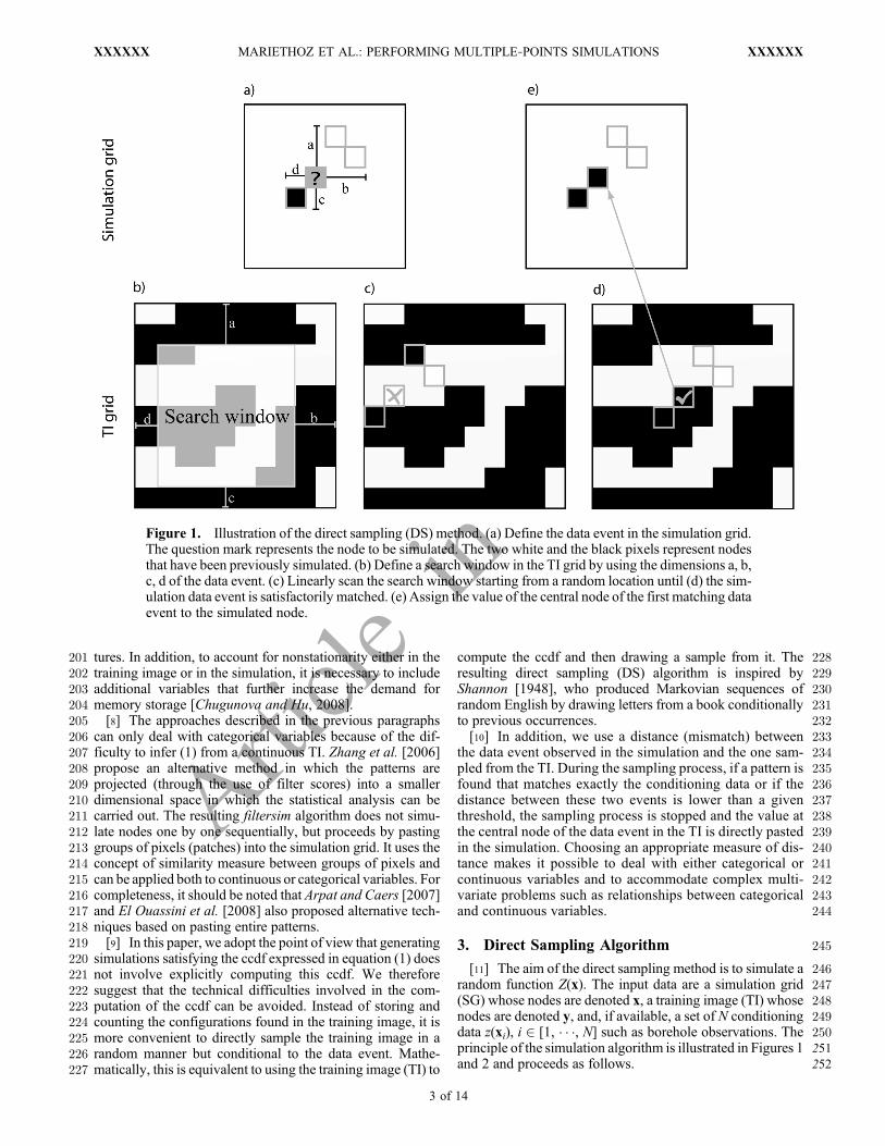
Figure 1. Illustration of the direct sampling (DS) method. (a) Define the data event in the simulation grid.The question mark represents the node to be simulated. The two white and the black pixels represent nodesthat have been previously simulated. (b) Define a search window in the TI grid by using the dimensions a, b,c, d of the data event. (c) Linearly scan the search window starting from a random location until (d) the sim-ulation data event is satisfactorily matched. (e) Assign the value of the central node of the first matching dataevent to the simulated node.


3 of 14

253 [12] 1. Each conditioning data is assigned to the closest254 grid node in the SG. If several conditioning data should be255 assigned to the same grid node, we assign the closest one to256 the center of the grid node.257 [13] 2. Define a path through the remaining nodes of the258 SG. The path is a vector containing all the indices of the grid259 nodes that will be simulated sequentially. Random [Strebelle,260 2002], unilateral (where nodes are visited in a regular order261 starting along one side of the grid [e.g. Daly, 2004]) or any262 other path can be used.263 [14] 3. For each successive location x in the path:264 [15] a. Find the neighbors of x. They consist of a maximum265 of the n closest grid nodes {x1, x2, � � �, xn} that were already266 assigned or simulated in the SG. If no neighbor is found for x267 (e.g., for the first node of an unconditional simulation), ran-268 domly take a node y in the TI and assign its value Z(y) to Z(x)269 in the SG. The algorithm can then proceed to the next node in270 the path.271 [16] b. Compute the lag vectors L = {h1, � � �, hn} = {x1 − x,272 � � �, xn − x} defining the neighborhood of x,N(x,L) = {x + h1,273 � � �, x + hn}. For example, in Figure 1a the neighborhood of274 the gray pixel (that represents the node to be simulated)275 consists of three lag vectors L = {(1, 2), (2, 1), (−1, 1)}276 corresponding to the relative locations of the three already277 simulated grid nodes.278 [17] c. Define the data event dn (x, L) = {Z(x + h1), � � �,279 Z(x + hn)}. It is a vector containing the values of the280 variable of interest at all the nodes of the neighborhood. In the281 example of Figure 1a, the data event is dn (x, L) = {0, 0, 1}.282 [18] d. Define the search window in the TI. It is the283 ensemble of the locations y such that all the nodesN(y,L) are284 located in the TI. The size of the search window is defined by285 the minimum and maximum values of the individual com-286 ponents of the lag vectors (Figure 1b).287 [19] e. Randomly draw a location y in the search window288 and from that location scan systematically the searchwindow.289 For each location y:290 [20] i. Find the data event dn(y, L) in the training image. In291 Figure 1c, a random grid node has been selected in the search292 window of the TI. The data event is retrieved and is found to293 be dn(y, L) = {1, 0, 1}.

294[21] ii. Compute the distance d{dn(x, L), dn(y, L)}295between the data event found in the SG and the one found296in the TI. The distance is computed differently for contin-297uous or discrete variables. Therefore we will describe this298step more in detail later in the paper.299[22] iii. Store y, Z(y) and d{dn(x, L), dn(y, L)} if it is the300lowest distance obtained so far for this data event.301[23] iv. If d{dn(x, L), dn(y, L)} is smaller than the accep-302tance threshold t, the value Z(y) is sampled and assigned to303Z(x). This step is illustrated in Figure 1d. In that case, the304current data event in the TI matches exactly the data event305in the SG. The distance is zero and the value Z(y) = 1 is306assigned to the SG (Figure 1e).307[24] v. If the number of iterations of the loop i–iv exceeds a308certain fraction of the size of the TI, the node ywith the lowest309distance is accepted and its value Z(y) is assigned to Z(x).310[25] The definition of the data event by considering the n311closest informed grid nodes is very convenient as it allows the312radius of the data events to decrease as the density of313informed grid nodes becomes higher. This natural variation of314the data events size has the same effect as multiple grids315[Strebelle, 2002] and makes their use unnecessary. Figure 2316illustrates the decrease of the data events radius with neigh-317borhoods defined by the four closest grid nodes.318[26] In the proposed method, the concept of a distance319between data events d{dn(x), dn(y)} is extremely powerful,320because it is flexible and can be adapted to the simulation of321both continuous and categorical attributes. For categorical322variables, we propose to use the fraction of nonmatching323nodes in the data event, given by the indicator variable a that324equals 0 if two nodes have identical value and 1 otherwise,

d dn xð Þ; dn yð Þf g ¼ 1

n

Xni¼1

ai 2 0;1½ �;

where ai ¼0 if Z xið Þ ¼ Z yið Þ1 if Z xið Þ 6¼ Z yið Þ

�: ð2Þ

325This measure of distance gives the same importance to all the326nodes of the data event regardless of their location relative to327the central node. It may be preferable to weight equation (2)328according to the distance of each node in the template from

Figure 2. Illustration of the natural reduction of the data events size. The neighborhoods for simulatingthree successive grid nodes a, b, and c are defined as the four closest grid nodes. As the grid becomes moredensely informed, the data events become smaller.


4 of 14

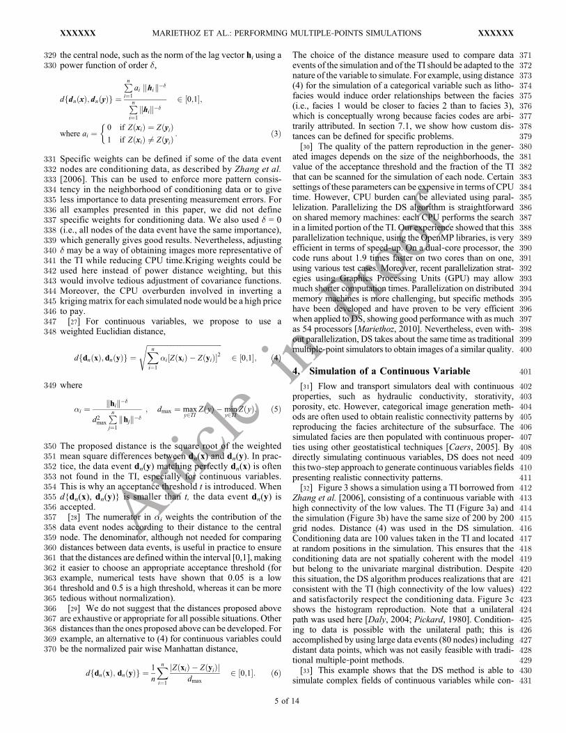
329 the central node, such as the norm of the lag vector hi using a330 power function of order d,

d dn xð Þ; dn yð Þf g ¼Pni¼1

ai khik��

Pni¼1

khik��

2 0;1½ �;

where ai ¼0 if Z xið Þ ¼ Z yið Þ1 if Z xið Þ 6¼ Z yið Þ

�: ð3Þ

331 Specific weights can be defined if some of the data event332 nodes are conditioning data, as described by Zhang et al.333 [2006]. This can be used to enforce more pattern consis-334 tency in the neighborhood of conditioning data or to give335 less importance to data presenting measurement errors. For336 all examples presented in this paper, we did not define337 specific weights for conditioning data. We also used d = 0338 (i.e., all nodes of the data event have the same importance),339 which generally gives good results. Nevertheless, adjusting340 d may be a way of obtaining images more representative of341 the TI while reducing CPU time.Kriging weights could be342 used here instead of power distance weighting, but this343 would involve tedious adjustment of covariance functions.344 Moreover, the CPU overburden involved in inverting a345 krigingmatrix for each simulated node would be a high price346 to pay.347 [27] For continuous variables, we propose to use a348 weighted Euclidian distance,

d dn xð Þ; dn yð Þf g ¼ffiffiffiffiffiffiffiffiffiffiffiffiffiffiffiffiffiffiffiffiffiffiffiffiffiffiffiffiffiffiffiffiffiffiffiffiffiffiffiffiffiffiffiXni¼1

�i Z xið Þ � Z yið Þ½ �2s

2 0;1½ �; ð4Þ

349 where

�i ¼ khik��

d2max

Pnj¼1

khjk��

; dmax ¼ maxy2TI

Z yð Þ �miny2TI

Z yð Þ: ð5Þ

350 The proposed distance is the square root of the weighted351 mean square differences between dn(x) and dn(y). In prac-352 tice, the data event dn(y) matching perfectly dn(x) is often353 not found in the TI, especially for continuous variables.354 This is why an acceptance threshold t is introduced. When355 d{dn(x), dn(y)} is smaller than t, the data event dn(y) is356 accepted.357 [28] The numerator in ai weights the contribution of the358 data event nodes according to their distance to the central359 node. The denominator, although not needed for comparing360 distances between data events, is useful in practice to ensure361 that the distances are defined within the interval [0,1], making362 it easier to choose an appropriate acceptance threshold (for363 example, numerical tests have shown that 0.05 is a low364 threshold and 0.5 is a high threshold, whereas it can be more365 tedious without normalization).366 [29] We do not suggest that the distances proposed above367 are exhaustive or appropriate for all possible situations. Other368 distances than the ones proposed above can be developed. For369 example, an alternative to (4) for continuous variables could370 be the normalized pair wise Manhattan distance,

d dn xð Þ; dn yð Þf g ¼ 1

n

Xni¼1

Z xið Þ � Z yið Þj jdmax

2 0;1½ �: ð6Þ

371The choice of the distance measure used to compare data372events of the simulation and of the TI should be adapted to the373nature of the variable to simulate. For example, using distance374(4) for the simulation of a categorical variable such as litho-375facies would induce order relationships between the facies376(i.e., facies 1 would be closer to facies 2 than to facies 3),377which is conceptually wrong because facies codes are arbi-378trarily attributed. In section 7.1, we show how custom dis-379tances can be defined for specific problems.380[30] The quality of the pattern reproduction in the gener-381ated images depends on the size of the neighborhoods, the382value of the acceptance threshold and the fraction of the TI383that can be scanned for the simulation of each node. Certain384settings of these parameters can be expensive in terms of CPU385time. However, CPU burden can be alleviated using paral-386lelization. Parallelizing the DS algorithm is straightforward387on shared memory machines: each CPU performs the search388in a limited portion of the TI. Our experience showed that this389parallelization technique, using the OpenMP libraries, is very390efficient in terms of speed‐up. On a dual‐core processor, the391code runs about 1.9 times faster on two cores than on one,392using various test cases. Moreover, recent parallelization strat-393egies using Graphics Processing Units (GPU) may allow394much shorter computation times. Parallelization on distributed395memory machines is more challenging, but specific methods396have been developed and have proven to be very efficient397when applied to DS, showing good performance with as much398as 54 processors [Mariethoz, 2010]. Nevertheless, even with-399out parallelization, DS takes about the same time as traditional400multiple‐point simulators to obtain images of a similar quality.

4014. Simulation of a Continuous Variable

402[31] Flow and transport simulators deal with continuous403properties, such as hydraulic conductivity, storativity,404porosity, etc. However, categorical image generation meth-405ods are often used to obtain realistic connectivity patterns by406reproducing the facies architecture of the subsurface. The407simulated facies are then populated with continuous proper-408ties using other geostatistical techniques [Caers, 2005]. By409directly simulating continuous variables, DS does not need410this two‐step approach to generate continuous variables fields411presenting realistic connectivity patterns.412[32] Figure 3 shows a simulation using a TI borrowed from413Zhang et al. [2006], consisting of a continuous variable with414high connectivity of the low values. The TI (Figure 3a) and415the simulation (Figure 3b) have the same size of 200 by 200416grid nodes. Distance (4) was used in the DS simulation.417Conditioning data are 100 values taken in the TI and located418at random positions in the simulation. This ensures that the419conditioning data are not spatially coherent with the model420but belong to the univariate marginal distribution. Despite421this situation, the DS algorithm produces realizations that are422consistent with the TI (high connectivity of the low values)423and satisfactorily respect the conditioning data. Figure 3c424shows the histogram reproduction. Note that a unilateral425path was used here [Daly, 2004; Pickard, 1980]. Condition-426ing to data is possible with the unilateral path; this is427accomplished by using large data events (80 nodes) including428distant data points, which was not easily feasible with tradi-429tional multiple‐point methods.430[33] This example shows that the DS method is able to431simulate complex fields of continuous variables while con-


5 of 14

432 straining properties such as the statistical distribution and the433 connectivity patterns. Therefore, the method can produce434 specific types of heterogeneity that control the flow and435 transport behavior of the model.

436 5. Multivariate Case

437 [34] Contrary to existing multiple‐point simulation tech-438 niques, DS is not limited by the dimension of the data events439 because there is no need to store their occurrences. Hence the440 data events can be defined through several variables that can441 be simulated jointly or used for conditioning following the442 same principle as cosimulation (it may be collocated or not).443 The training image is a multivariate field comprising m444 variables Z1(x), � � �, Zm(x). Such multivariate fields are pre-445 sented as “vector images” by Hu and Chugunova [2008].446 Accounting for multiple‐point dependence between variables447 means to respect cross correlations between all combinations448 of nodes within multivariate data events. The conditional449 cumulative density function (1) for the variable Zk is then450 expressed as

Fk z; x; d1n1 ; � � � ; dmnm� �

¼ Prob Zk xð Þ � zjd1n1 ; � � � ; dmnmn o

;

k ¼ 1; � � � ;m: ð7Þ

451 Each variable Zk involved in the multivariate analysis can452 have a different neighborhood and a specific data event453 dnk

k (x, Lk) = {Zk(x + h1k), � � �, Zk(x + hnk

k )}. The number nk454 of nodes in the data event of each variable can be different,455 as well as the lag vectors Lk. To simplify the notation, we just456 extend the previous concept of data event to the multivariate457 case: here the data event dn(x) is the joint data event

458including all the individual data events dn(x) = {dn11 (x, L1),

459� � �, dnmm (x, Lm)}. The distance between a joint data event460found in the simulation and one found in the TI is defined461as a weighted average of the individual distances defined

previously,

d dn xð Þ; dn yð Þf g ¼Xmk¼1

wkd dknk x;Lk� �

; dknk y;Lk� �n o

2 0;1½ �;

withXmk¼1

wk ¼ 1; and wk � 0: ð8Þ

462The weights wk are defined by the user. They can for the463fact that the pertinent measure of distance may be different464for each variable. Multivariate simulations are performed465using a single (random) path that visits all components of466vector Z at all nodes of the SG.467[35] Figure 4 shows an example of a joint simulation of two468variables that are spatially Dependent by some unknown469function. For this synthetic example, the TI for variable 1470(Figure 4a) is a binary image representing a channel system471[Strebelle, 2002]. The TI for variable 2 (Figure 4b) was ob-472tained by smoothing variable 1 using a moving average with a473window made of the 500 closest nodes and then adding an474uncorrelated white noise uniformly distributed between 0 and4750.5. This secondary variable could represent the resistivity476map corresponding to the lithofacies given by variable 1. The477result is a bivariate training image where variables 1 and 2 are478related via a multiple‐point dependency. Figures 4c and 4d479show one unconditional bivariate simulation using the TI480described above. The categorical variable 1 uses distance (3)

Figure 3. Illustration of the method using a continuous variable. (a) Training image with continuousvariable. (b) One simulation using the unilateral path with 100 randomly located conditioning data (n =80, t = 0.01). Positions of conditioning data are marked by circles whose colors indicate the values of thedata. (c) Comparison of the histograms.


6 of 14

481 and the continuous variable 2 uses distance (4). The multiple‐482 point dependence relating both variables is well reproduced,483 both visually and in terms of cross variograms (Figure 4e),484 which is a measure of two‐point correlation. Note that ad-485 dressing dependencies between categorical and continuous486 variables is usually awkward. The scatter plot depends on the487 facies numbering (which is arbitrary) and correlation factors488 are meaningless. Here DS is able to reproduce multiple‐point489 dependence, including statistical parameters more complex490 than the scatterplot (e.g., cross variograms).491 [36] Problems traditionally addressed by including492 exhaustively known secondary variables [e.g., Mariethoz493 et al., 2009] are particular cases of the multivariate DS494 approach. Whereas existing MP methods consider only the495 secondary variable at the central node x, DS accounts for496 complex spatial patterns of the secondary variable because497 multiple‐point statistics are considered for both primary and498 secondary variables.

499[37] When one (or several) of the joint variables is already500known, DS uses this information as indirect conditioning data501(secondary variable) guiding the simulation of the other502variables (primary variables) and then reducing uncertainty.503In the following example, the aim is to simulate the pri-504mary variable knowing only the secondary variable and the505multiple‐point statistical relationship between primary and506secondary variables, which is given via the bivariate TI. For507illustration, consider Figures 4a and 4b as the bivariate TI508and Figure 5b as the auxiliary variable for the simulation509grid. Figure 5b was obtained as follows. First, Figure 5a was510generated with an univariate unconditional simulation using511Figure 4a as TI. Then, Figure 5b was computed from512Figure 5a, applying a moving average followed by addition513of a white noise. Hence, the aim is to reconstruct the ref-514erence field Figure 5a from Figure 5b and the multiple‐point515dependence given by the bivariate TI (Figures 4a and 4b),516using multivariate DS.

Figure 4. Joint simulation of two variables (n1 = 30, n2 = 30, t = 0.01, w1 = 0.5, w2 = 0.5). (a and b) Thebivariate training image, with a complex multiple‐point dependence. (c and d) One resulting bivariate sim-ulation, where the MP dependence is reproduced. (e) Cross‐variograms reproduction. Note that no vario-gram adjustment was necessary.


7 of 14

517 [38] Figure 5c displays one realization of the primary518 variable, conditional to the exhaustively known secondary519 variable (Figure 5b). No conditioning data are available for520 the primary variable. The features of the reference field are521 correctly inferred from the information contained in the sec-522 ondary variable, as shown in Figure 5d, where the reference523 (Figure 5a) and the simulation (Figure 5c) are superposed. In524 Figure 5e, the mean of 100 simulations is presented. In525 average, the channels are correctly located when compared to526 the reference.527 [39] This technique could be applied for example, when a528 ground penetrating radar survey provides an exhaustive data529 set (secondary variable) and when the primary variable that530 needs to be characterized is the hydraulic conductivity [e.g.,531 Langsholt et al., 1998]. The relation between both variables is532 complex and not necessarily linear. DS can be applied to this533 type of problem if one can provide a bivariate TI. A possi-534 bility to construct the bivariate TI is to use first a TI of the535 hydraulic conductivity and then use a forward geophysical536 model to simulate the secondary variable.

537 6. Dealing With Nonstationarity

538 [40] Geological processes are intrinsically nonstationary.539 The ability to address nonstationarity is vital for the appli-

540cability of a geostatistical method in Earth Sciences. For541existing MP methods, several techniques can be found in the542literature to account for nonstationarity either of the TI or of543the simulated field [Chugunova andHu, 2008;De Vries et al.,5442009; Journel, 2002; Strebelle, 2002]. One of the ways of545dealing with nonstationary TIs is to divide a nonstationary TI546in stationary zones, each considered as a separate stationary547TI [Boucher, 2009; De Vries et al., 2009]. The simulation548domain is then also divided into zones, each corresponding to549a specific TI. In the framework of traditional multiple‐point550statistics, usingmultiple TIs involves creating one data events551catalogue per training image [Wu et al., 2008]. Although, it552may be difficult in practice to define the stationary zones, it553could be applied easily with DS by scanning a different part of554a TI or different TIs for each simulated zone. There would be555no limitations to the number of TIs and zones related to556memory requirements. More generally, all the techniques557cited above can be used with DS, but new possibilities are558also offered by exploiting the specificities of DS.

5596.1. Addressing Nonstationarity With Specific560Distances

561[41] We discussed above how the distance measure should562be chosen according to the nature of the variables at stake.

Figure 5. The use of a secondary variable to guide the simulation of a primary variable. (a) The referenceprimary variable, obtained with a univariate unconditional simulation using Figure 4a as TI. (b) The ref-erence secondary variable computed by transformations of the primary variable (see text for details). Thebivariate training images a and b describe the MP relationship between primary and secondary variables.(c) One multivariate simulation generated using the fully known secondary variable b as conditioningdata (n1 = 30, n2 = 30, t = 0.01, w1 = 0.5, w2 = 0.5). (d) Superposition of one simulation and the reference.(e) Mean of 100 simulations.


8 of 14

563 Following this idea, we propose to forge distances adapted to564 nonstationary cases. An example of such custom distance565 measure is the pair‐wise Euclidean distance relative to the566 mean of the data event,

d dn xð Þ; dn yð Þf g

¼Xni¼1

�i Z xið Þ � �Z xð Þð Þ � Z yið Þ � �Z yð Þð Þ½ �2 !1=2

2 0;1½ �;

ð9Þ

567 with Z xð Þ ¼ 1n

Pni¼1

Z(xi). When a matching data event is found

568 in the TI, the local mean of the SG data event is added to the569 value found in the TI. Therefore, the value Z(y) − Z(y) + Z(x)570 is attributed to the simulated node. The distance described in571 equation (9) compares data events by their relative varia-572 tions only and not their actual values. This variation‐based573 distance can be very useful when considering first‐order574 nonstationary phenomena. We illustrate this situation with575 the example depicted in Figure 6. The available training576 image (Figure 6a) is a multi‐Gaussian field with zero mean577 and unit variance, resulting in minimum and maximum578 values of −3.52 and 3.99, respectively. It was generated579 using an exponential variogram model, with ranges of 35580 units along the x axis and 25 units along the y axis. Its size is581 250 by 250 grid nodes. One hundred conditioning data are582 available (Figure 6b), but they are not compatible with the583 training image, as their values span between a minimum of584 99.55 and a maximum of 110.92, with a mean of 105.12.585 Moreover, these data show nonstationarity. Because the586 distance (9) is based on the variations of the values in the587 data event, it is possible to find matches between the data588 events found in the data and the ones of the TI despite the589 difference in the range and the nonstationarity. The resulting590 simulations (one is shown in Figure 6c) display the same591 variable range (minimum, 98.13; maximum, 111.72; mean,592 104.87) and the same nonstationary behavior as the data, but593 also a spatial structure similar to what is found in the TI. In594 this case, nonstationarity can be seen as a locally varying595 mean, and therefore distance (9) can accommodate it well. If596 the nonstationarity was more complex, such as, for example,597 structures ranging from channels to lenses, this distance598 measure would not be appropriate.

599[42] This example shows that variation‐based distance can600be used when a conceptual model allows the geologist to601provide a training image, but when the data indicate the602presence of nonstationarity and inadequacy of the ranges603given in the TI. Moreover, it emphasizes the flexibility604offered by using distances between data events, which is one605of the major advantages of the DS approach.

6066.2. Addressing Nonstationarity With Transformation607of Data Events

608[43] Traditional multiple‐point simulation implementa-609tions such as snesim include the possibility of imposing610transformations on the structures found in the TI. This is done611by first constructing the data events catalogue using a trans-612formed template and then simulating values with a non-613transformed template [Strebelle, 2002]. The most commonly614implemented transformations are rotation and affinity615(application of homothetic transformations on the template).616This feature is very useful when the modeler has a single617stationary training image and wants to use it for the simula-618tion of nonstationary fields. If many different transformations619have to be applied on the simulation grid, most approaches620store as many data events catalogues. The DS approach also621allows these transformations. Simply scanning the TI with a622transformed data event gives the same results as the tradi-623tional technique. Moreover, transformations are not defined624by zones, but as a continuum, because the transformation can625be different for each simulated node. In some cases, rotation626or affinity may result in large data events that do not fit in the627TI. In such cases, the data event nodes located outside of the628TI are ignored until it becomes possible to scan the TI with629this new, reduced data event.630[44] Figure 7 shows an example of such transformation,631with angle and affinity maps (Figures 7a and 7b) defined by632continuous variables. All angles between −180° and 180° are633represented, and the affinity ratios range from 1 at the center634of the image to 0.4 in the corners (meaning that all structures635are reduced to 40% of the size they have in the TI). The636training image (Figure 7c) is much smaller (250 by 250637nodes) than the simulation domain (1000 by 1000 nodes) and638represents horizontal channels. This combined transforma-639tion (rotations + affinities) results in channels oriented in all

Figure 6. Simulation using a variation‐based distance. (a) Multi‐Gaussian stationary training image.(b) Nonstationary data set (100 points data), with values in a different range than those of the training image.(c) One simulation with variation‐based distance (n = 15, t = 0.01). Circles represent the location of the 100conditioning data.


9 of 14

640 directions and becoming thinner as they are located further641 away from the centre (Figure 7d).

642 6.3. Addressing Nonstationarity With a Secondary643 Variable

644 [45] A situation where a secondary variable can be645 extremely powerful occurs when the training image itself is646 nonstationary. This is the case, for example, when the TI is647 taken from direct field observation or when it is obtained from648 a process based simulation. When this type of nonstationarity649 occurs, one can introduce one or several secondary variables650 to model the nonstationarity in the TI and in the simulation, as651 it was proposed by Chugunova and Hu [2008]. The approach652 uses spatially continuous auxiliary variables to distinguish653 the regions where similar patterns occur. This secondary654 variable can be rather abstract, it just needs to be defined on655 the training image and on the simulation grid and it must have656 similar values in regions where similar patterns occur. While657 this idea was implemented by Chugunova and Hu [2008] by658 modifying the probability tree structure of snesim, it is659 accomplished in a straightforward manner with DS by using a660 multivariate TI with variable 1 being the variable of interest

661and the other variables describing the non‐stationarity of662variable 1.663[46] Figure 8 illustrates this concept in a simple situation.664The TI for the primary variable is binary and shows a set of665rotating channels. The orientation of the channels changes as666a function of the X coordinate (Figure 8a). Therefore, a simple667way to describe this nonstationarity is to use the X coordinate668as the secondary variable (Figure 8b). On the simulation, if669ones want to have horizontal channels on the top, vertical670channels in the bottom and a smooth transition in between,671one first generates a map of the secondary variable such as the672values of this map describe the required nonstationarity: in673this case, the secondary variable (X coordinate map) is rotated674so that zeros are at the bottom, ones are on top, and inter-675mediate values are in between (Figure 8d). Using that sec-676ondary information and the standard multivariate collocated677cosimulation DS method presented earlier, the resulting678simulation displays the desired non‐stationary behavior679(Figure 8c). For these simulations, the neighborhoods are680made of n1 = 30 nodes for the primary variable and n2 = 1 for681the secondary variable, because a single node is enough to682characterize the nonstationarity. The weights of both vari-683ables are kept equal, with w1 = w2 = 0.5.

Figure 7. Transformations of the data events. (a) Rotation map. (b) Affinity map. (c) Stationary trainingimage. (d) Simulation with transformed data events (n = 30, t = 0).


10 of 14

684 [47] Although this is a simple example, the use of a con-685 tinuous secondary variable to describe nonstationarity allows686 accounting for very rich types of nonstationarity such as a687 change in the type of structures encountered.

688 7. Improving Pattern Reproduction

689 [48] Accurate pattern reproduction can be jeopardized690 when a data event cannot be found in the TI. This problem is691 common to all multiple‐point simulations methods and is692 more acute when a random path is used in the simulation grid.693 In traditional multiple‐point simulation algorithms, this issue694 is usually dealt with by dropping the neighbor node that is the695 farthest away from the central node and, by performing a696 search in the data events catalogue for this new, reduced697 pattern [Strebelle, 2002]. The main drawback of this proce-698 dure is that it induces a degradation of the pattern reproduc-699 tion by artificially reducing the template size for the com-700 putation of the ccdf (1). Such degradation can lead to a lack of701 spatial continuity of the simulated structures (such as chan-702 nels). Several authors have proposed methods to improve703 patterns reproduction. Strebelle and Remy [2005] locate the704 nodes that were simulated using a reduced neighborhood and705 resimulate the dropped neighbors at the end of each multigrid706 step. This method does not remove all the inconsistencies in707 the simulated patterns but performs additional simulation708 attempts with updated neighborhoods. As problematic values709 are temporarily accepted (until the entire multigrid is simu-710 lated), they propagate inconsistencies to nodes that are sim-

711ulated later. Therefore, if a node is successfully resimulated, it712is not guaranteed that all its neighbors are consistent between713each other. Another algorithm, proposed by Stien et al.714[2007], does not temporarily accept values generating con-715flicts but deletes the problematic nodes in the neighborhood.716At the end of a multigrid level, these nodes are simulated. The717process is iterative and needs specific parameters to ensure718convergence. Although this method avoids the propagation of719inconsistencies by deleting them, it does not resolve the720problem of the origin of these problematic patterns. Indeed,721inconsistencies exist because other nearby problematic pat-722terns occurred previously in the simulation process. In our723opinion, the only way to deal with this problem is to imme-724diately address the entire cascade of causes at the origin of725problematic patterns.726[49] In the context of simulations using a unilateral path727[Daly, 2004], Suzuki and Strebelle [2007] developed the real‐728time postprocessing method (RTPP) that walks back the729unilateral path when problematic neighborhoods are730encountered and resimulates the most recent nodes until the731produced patterns satisfactorily match the ones of the TI. The732limits of this method are that it is applicable to the first stage733of the simulation only (the first multigrid) and only when734using a unilateral path. Therefore, like all simulation methods735using the unilateral model, it suffers from difficulties in736honoring conditioning data. Nevertheless, this method has the737advantage of correcting all inconsistencies because it738resimulates the neighborhoods of the problematic nodes and

Figure 8. The use of a secondary variable to model nonstationarity. (a) Variable 1 of nonstationary train-ing image. (b) Dependent joint variable describing the nonstationarity of variable 1 in training image.(c) Resulting simulation for variable 1 (n1 = 30, n2 = 1, t = 0.01, w1 = 0.5, w2 = 0.5). (d) Dependent jointvariable (exhaustively known) describing the nonstationarity of variable 1 in simulation.


11 of 14

739 not only the problematic nodes themselves. As incon-740 sistencies are resimulated immediately, it avoids propagation741 to their neighbors.742 [50] In this context, we propose a new algorithm, the syn‐743 processing, aimed at improving the reproduction of patterns.744 It is generic enough to be applicable to any type of path and745 with or without multigrids. As the RTPP, it resimulates values746 as soon as inconsistencies are met. It is based on the idea that747 when an inconsistent pattern (with respect to the TI) is found,748 it is because other inconsistencies occurred previously in the749 simulation process. Therefore, before resimulating problem-750 atic nodes, their neighborhoods also need to be (at least751 partially) resimulated. If inconsistencies appear during this752 resimulation, further resimulation needs to be performed.753 Hence, the algorithm is of a recursive nature.754 [51] The syn‐processing algorithm consists in the follow-755 ing steps at each simulated node x: check if the simulated756 value Z(x) is acceptable. The acceptance criterion can be a757 minimum number of dropped neighbor nodes in the frame-758 work of classical multiple‐point implementation. In the case759 of DS, the criterion is that the minimum distance d{dn(x),760 dn(y)} found is below a threshold.761 [52] If the criterion is not met, the simulation of Z(x) is762 postponed and one of its neighbors N−1(x), taken among763 those that do not belong to the original set of conditioning764 data, is resimulated taking into account the same criterion. For765 the simulation of the node N−D(x):766 [53] 1. If the criterion is not met for Z{N−D(x)}, delete it767 and resimulate one of its neighbors, N−(D+1)(x).768 [54] 2. If the criterion is met for Z{N−D(x)}, accept this769 value and try simulating Z{N1−D(x)}.770 [55] Note that D is the number of deleted nodes for the771 initial node x. To ensure convergence, a maximum allowed772 number of deletions must be set.773 [56] Syn‐processing can sometimes delete and resimulate774 the same nodes in a cyclic manner. Such cycles are a waste of775 time as they do not improve the simulation. This can be776 avoided by keeping a record of all deletions. Before each777 deletion, the analysis of this record allows finding if the778 present state of the SG already occurred in the past. If it is the779 case, another random neighbor is chosen in order to break the780 cycle.781 [57] Tests show that syn‐processing efficiently improves782 pattern reproduction, as well as conditioning to local data. As783 the algorithm is recursive, CPU time can be adversely784 affected depending on the criterion to accept a simulated785 value. If the criterion is very strict (such as t = 0 for a con-786 tinuous variable) and if the maximum allowed number of787 iterations is very large, convergence can be compromised. On788 the other hand, improving pattern reproduction increases the789 global coherence of the simulation with respect to the TI. It790 becomes then easier to find matching data events in the TI,791 thus making the scan process faster for the remaining nodes.792 In certain cases, syn‐processing can even reduce simulation793 time up to a factor 2 while improving simulations quality.794 Moreover, tests showed that performing syn‐processing only795 at the beginning of the simulation is sufficient to obtain better796 reproduction of large‐scale features and general connected-797 ness of the simulated structures, as compared to simulations798 without syn‐processing. Therefore, a tradeoff needs to be799 achieved between the different parameters governing the800 simulation, in order to obtain optimal results at the lowest801 possible CPU cost.

802[58] Note that syn‐processing was used when generating803the simulation examples presented in Figures 5a and 8. For804comparison, note the difference of continuity between805Figure 4c, where no syn‐processing was used, and Figure 5a806that was generated using syn‐processing. The latter figure807reproduces better the sinuosity and the connectivity of the808channels found in the TI.

8098. Discussion and Conclusion

810[59] In this paper, we presented the direct sampling (DS)811simulation method and a recursive syn‐processing algo-812rithm to enhance the quality of pattern reproductions in the813simulations.814[60] As compared to traditional multiple point techniques815such as snesim [Strebelle, 2002], the proposed method is able816to generate exactly the same ensemble of stochastic realiza-817tions if we use the same neighborhood as snesim and if we use818multigrids. The advantage of DS is that it allows respecting819the conditional probability distribution that could be com-820puted from the training image without having to actually821compute it. Because it is not necessary to estimate this con-822ditional probability distribution, the method can be applied in823situations where the traditional approach failed such as very824large number of facies, continuous variables or multivariate825cases. In addition, when a classical multiple‐point technique826does not find a certain data configuration in a TI, it usually827drops successive data points from the data event until it finds828a configuration that exists in the TI. This procedure may be829rather arbitrary. Here we avoid this practice by using a dis-830tance between two data events.When the data event cannot be831found exactly, we select one data event that is acceptable832within a predefined error range. The distance threshold833between data events is an additional parameter that allows to834control the model and how the DS will reproduce the patterns835found in the TI. Setting this threshold above a value 0 means836that the user accepts differences between the TI and the837simulation. This clearly shows that the probabilistic model838proposed in this work is a numerical model that includes not839only the TI but also the acceptance threshold as well as the840number of neighbors and any additional parameters that841needs to be defined when accounting for nonstationarity. The842validity of a particular model based on the DS method, like843the validity of any stochastic model, can then be tested by844standard cross‐validation techniques on any real data set. This845classical approach can be used to select the best model846amongst a series of possible TI and parameter sets and also to847compare its performances with other more standard stochastic848models.849[61] By using distances between data events, DS offers the850possibility to use training images that can either be categorical851or continuous, uni‐ or multivariate, stationary or nonsta-852tionary. This can be extremely powerful when realistic geo-853logical structures must be modeled, as is commonly the case854for hydrogeological problems like contaminant migration,855which are strongly influenced by heterogeneity and connec-856tivity of the geological structures.857[62] The multivariate framework offered by DS opens new858perspectives for the integration of different data types in859groundwater and surface hydrology. By accounting for860multiple‐point dependence between several variables, DS can861exploit nonparametric relationships between variables of862different nature, such as between categorical and continuous


12 of 14

863 variables. Possible applications can be very diverse since864 categorical variables (e.g., geology, soil type, land cover865 category, vulnerability class) and continuous variables (e.g.,866 porosity, concentration, recharge rate, rainfall) are often867 related and widely used in hydrology but are very seldom868 measured exhaustively. Therefore, these variables often must869 be interpolated. The DS method could then be used in this870 context.871 [63] In addition to the wide spectrum of potential appli-872 cations, DS has computational advantages that make it easier873 to apply than traditional multiple‐point methods. DS mas-874 sively reduces memory usage because no catalogue of data875 events needs to be stored. This implies that the size of the876 neighborhood is not limited by memory considerations. The877 data event can be spread across many different variables,878 allowing to perform multivariate simulations of variables879 presenting complex multiple‐point dependence.880 [64] Because multiple‐point statistics are not stored, DS881 does not need a fixed geometry of the data events. The shape882 of the data event can change at each simulated node and so883 can the search window. Hence, the data events are always884 adapted to the simulation path. The size of the data events is885 only limited by the size of the TI and is controlled by a886 maximum number n of nodes. In certain cases, it can be useful887 to limit the radius of the data events, for example, when888 considering nonstationary variables, to avoid capturing non-889 stationarity within the data events. It is also useful if the890 simulation is larger than the training image. In this case, very891 large data events can result in very small search windows,892 leading to a bias toward reproducing the statistical properties893 of a small central portion of the TI.894 [65] A related advantage of the DS approach is that mul-895 tigrids (a step‐like decrease in the template dimension) are896 replaced by a progressive (linear) decrease of the size of the897 data event as a function of the density of simulated nodes. It898 ensures that structures of all sizes are present in the simula-899 tion. Abandoning multigrids avoids problems related to the900 migration of conditioning data on coarse multigrid levels. By901 avoiding multigrids, DS is easy to implement, easy to902 parameterize and has no problems accommodating large data903 sets.904 [66] A very important point is that DS does not require905 prohibitive CPU time, with performances comparable to ex-906 isting methods. This good performance is possible because907 the algorithm searches only a single matching data event, and908 therefore, the whole TI often does not need to be scanned.909 There is a tradeoff between CPU time and the quality of the910 generated images, controlled by parameters such as the size of911 the neighborhoods, the value of the acceptance threshold and912 the fraction of the TI that can be scanned for the simulation of913 each node. However, using parallelization allows easily914 increasing the performance of DS.915 [67] The algorithms described in this paper are the object of916 an international patent application (PCT/EP2008/009819).

917 [68] Acknowledgments. We thank the Swiss National Science Foun-918 dation (grants PP002‐1065557 and PBNEP2‐124334) and the Swiss Con-919 federation’s Innovation Promotion Agency (CTI project 8836.1 PFES‐ES)920 for funding this work. We also thank Roland Froidevaux, Pierre Biver, Tati-921 ana Chugunova, Denis Allard, Olivier Besson, Alexandre Boucher, Jef922 Caers, Jesus Carrera, Peter Atkinson, Lin Hu, André Journel, and anonymous923 reviewers for their comments and advices.

924References925Aitokhuehi, I., and L. J. Durlofsky (2005), Optimizing the performance of926smart wells in complex reservoirs using continuously updated geological927models, J. Petrol. Sci. Eng., 48(3–4), 254–264.928Alcolea, A., P. Renard, G. Mariethoz, and F. Bretone (2009), Reducing the929impact of a desalination plant using stochastic modeling and optimization930techniques, J. Hydrol., 365(3–4), 275–288, doi:10.1016/j.jhydrol.9312008.11.034.932Alcolea, A., and P. Renard (2010), The blocking moving window sampler:933Conditioning multiple‐point simulations to hydrogeological data, Water934Resour. Res., 46, W08511, doi:10.1029/2009WR007943.935Arpat, B., and J. Caers (2007), Conditional simulations with patterns,Math.936Geol., 39(2), 177–203.937Boucher, A. (2007), Algorithm‐Driven and Representation‐Driven Ran-938dom Function: A New Formalism for Applied Geostatistics, Stanford939Cent. for Reservoir Forecast., Palo Alto, Calif.940Boucher, A. (2009), Considering complex training images with search tree941partitioning, Compute. Geosci., 35(6), 1151–1158.942Caers, J., S. Strebelle, and K. Payrazyan (2003), Stochastic integration of943seismic data and geologic scenarios: A West Africa submarine channel944saga, Leading Edge, 22(3), 192–196.945Caers, J. (2005), Petroleum Geostatistics, 88 pp., Soc. of Petroleum Eng.,946Richardson.947Caers, J., and T. Hoffman (2006), The probability perturbation method: A948new look at Bayesian inverse modeling, Math. Geol., 38(1), 81–100.949Capilla, J., and C. Llopis‐Albert (2009), Gradual conditioning of non‐950Gaussian transmissivity fields to flow and mass transport data: 1. Theory,951J. Hydrol., 371, 66–74.952Chugunova, T., and L. Hu (2008), Multiple‐point simulations constrained953by continuous auxiliary data, Math. Geosci., 40(2), 133–146.954Dagan, G. (1976), Stochastic conceptual analysis of one‐dimensional955groundwater flow in nonuniform homogeneous media—Comment,956Water Resour. Res., 12(3), 567–567, doi:10.1029/WR012i003p00567.957Dagan, G. (1986), Statistical theory of groundwater flow and transport:958Pore to laboratory, 25 laboratory to formation, and formation to regional scale,959Water Resour. Res., 22, 120S–134S, doi:10.1029/WR022i09Sp0120S.960Dagan, G. (1989), Flow and Transport in Porous Formations, Springer,961Berlin, Germany.962Dagan, G. (2004), On application of stochastic modeling of groundwater963flow and transport, Stochastic Environ. Res. Risk Assess., 18(4), 266–267.964Daly, C. (2004), Higher order models using entropy, Markov random fields965and sequential simulation, paper presented at Geostatistics Banff 2004,966Kluwer Acad., Banff, Alberta.967De Marsily, G., F. Delay, J. Gonçalvès, P. Renard, V. Teles, and S. Violette968(2005), Dealing with spatial heterogenity, Hydrogeol. J., 13(1), 161–183.969De Vries, L., J. Carrera, O. Falivene, O. Gratacos, and L. Slooten (2009),970Application of multiple point geostatistics to non‐stationary images,971Math. Geosci., 41(1), 29–42.972El Ouassini, A., A. Saucier, D. Marcotte, and B. Favis (2008), A patchwork973approach to stochastic simulation: A route towards the analysis of mor-974phology in multiphase systems, Chaos Sol. Frac., 36, 418–436.975Emery, X. (2007), Using the Gibbs sampler for conditional simulation of976Gaussian‐based random fields, Compute. Geosci., 33, 522–537.977Feyen, L., and S. Gorelick (2004), Reliable groundwater management in978hydroecologically sensitive areas, Water Resour. Res., 40, W07408,979doi:10.1029/2003WR003003.980Feyen, L., and J. Caers (2006), Quantifying geological uncertainty for flow981and transport modelling in multimodal heterogeneous formations, Adv.982Water Resour., 29(6), 912–929.983Freeze, R. A. (1975), A stochastic‐conceptual analysis of one dimensional984groundwater flow in nonuniform homogemeous media, Water Resour.985Res., 11(5), 725–741, doi:10.1029/WR011i005p00725.986Freeze, R. A., J. Massmann, L. Smith, T. Sperling, and B. James (1990),987Hydrogeological decision analysis: 1. A framework, Ground Water,98828(5), 738–766.989Gelhar, L. (1993), Stochastic SubsurfaceHydrology, PrenticeHall, Englewood990Cliffs, NJ.991Gómez‐Hernández, J. J., and X.‐H. Wen (1998), To be or not to be multi‐992Gaussian? A reflection on stochastic hydrogeology, Adv. Water Resour.,99321(1), 47–61.994Guardiano, F., and M. Srivastava (1993), Multivariate geostatistics:995Beyond bivariate moments, in Geostatistics‐Troia, edited by A. Soares,996pp. 133–144, Kluwier Acad., Dordrecht, Netherlands.997Hoffman, B. T., and J. Caers (2007), History matching by jointly perturbing998local facies proportions and their spatial distribution: Application to a999North Sea reservoir, J. Petrol. Sci. Eng., 57(3–4), 257–272.


13 of 14

1000 Hu, L., and T. Chugunova (2008), Multiple‐point geostatistics for model-1001 ing subsurface heterogeneity: A comprehensive review, Water Resour.1002 Res., 44, W11413, doi:10.1029/2008WR006993.1003 Huysmans, M., and A. Dassargues (2009), Application of multiple‐point1004 geostatistics on modelling groundwater flow and transport in a cross‐1005 bedded aquifer (Belgium), Hydrogeol. J., 17, 1901–1911.1006 Journel, A. (1983), Nonparametric estimation of spatial distributions, Math.1007 Geol., 15(3), 445–468.1008 Journel, A. (2002), Combining knowledge fromdiverse sources: An alternative1009 to traditional data independence hypotheses, Math. Geol., 34(5), 573–596.1010 Journel, A., and T. Zhang (2006), The necessity of a multiple‐point prior1011 model, Math. Geol., 38(5), 591–610.1012 Kerrou, J., P. Renard, H.‐J. Hendricks‐Franssen, and I. Lunati (2008), Issues1013 in characterizing heterogeneity and connectivity in non‐multi‐Gaussian1014 media, Adv. Water Resour., 31(1), 147–159.1015 Klise, K., G. Weissmann, S. McKenna, E. Nichols, J. Frechette,1016 T. Wawrzyniec, and V. Tidell (2009), Exploring solute transport and1017 streamline connectivity using lidar‐based outcrop images and geostatistical1018 representations of heterogeneity, Water Resour. Res., 45, W05413,1019 doi:10.1029/2008WR007500.1020 Knudby, C., and J. Carrera (2005), On the relationship between indicators1021 of geostatistical, flow and transport connectivity, Adv. Water Resour.,1022 28(4), 405–421.1023 Koltermann, C., and S. Gorelick (1996), Heterogeneity in sedimentary1024 deposits: A review of structure‐imitating, process‐imitating, and descrip-1025 tive approaches, Water Resour. Res., 32(9), 2617–2658, doi:10.1029/1026 96WR00025.1027 Langsholt, E., N. Kitterød, and L. Gottschalk (1998), Development of1028 three‐dimensional hydrostratigraphical architecture of the unsaturated1029 zone based on soft and hard data, Ground Water, 36(1), 104–111.1030 Liu, Y., A. Harding, W. Abriel, and S. Strebelle (2004), Multiple‐point1031 simulation integrating wells, three‐dimensional seismic data, and geol-1032 ogy, AAPG Bull., 88(7), 905–921.1033 Mariethoz, G., P. Renard, and R. Froidevaux (2009), Integrating collocated1034 auxiliary parameters in geostatistical simulations using joint probability1035 distributions and probability aggregation, Water Resour. Res., 45,1036 W08421, doi:10.1029/2008WR007408.1037 Mariethoz, G. (2010), A general parallelization strategy for random path1038 based geostatistical simulation methods, Compute. Geosci., 37(7),1039 953–958, doi:10.1016/j.cageo.2009.11.001.1040 Mariethoz, G., and P. Renard (2010), Reconstruction of incomplete data1041 sets or images using direct sampling, Math. Geosci., 42(3), 245–268,1042 doi:10.1007/s11004-010-9270-0.1043 Matheron, G. (1966), Structure et composition des perméabilités, Rev. de1044 l’IFP, 21, 564–580.1045 Matheron, G. (1967), Eléments Pour Une Théorie Des Milieux Poreux,1046 Masson, Paris.1047 Michael, H., A. Boucher, T. Sun, J. Caers, and S. Gorelick (2010), Com-1048 bining geologic‐process models and geostatistics for conditional simula-1049 tion of 3‐D subsurface heterogeneity, Water Resour. Res., 46, W05527,1050 doi:10.1029/2009WR008414.1051 Neuwiler, I., and O. Cirpka (2005), Homogenization of Richards equation1052 in permeability fields with different connectivities, Water Resour. Res.,1053 41, W02009, doi:10.1029/2004WR003329.1054 Pickard,D. (1980), UnilateralMarkov fields,Adv. Appl. Probab., 12, 655–671.1055 Renard, P. (2007), Stochastic hydrogeology: What professionals really1056 need?, Ground Water, 45(5), 531–541.1057 Ronayne, M., S. Gorelick, and J. Caers (2008), Identifying discrete geo-1058 logic structures that produce anomalous hydraulic response: An inverse1059 modeling approach, Water Resour. Res., 44, W08426, doi:10.1029/1060 2007WR006635.

1061Rubin, Y. (2003), Applied Stochastic Hydrogeology, 391 pp., Oxford Univ.1062Press, New York.1063Sanchez‐Vila, X., A. Guadagnini, and J. Carrera (2006), Representative1064hydraulic conductivities in saturated groundwater flow, Rev. Geophys.,106544, RG3002, doi:10.1029/2005RG000169.1066Sánchez‐Vila, X., J. Carrera, and J. P. Girardi (1996), Scale effects in trans-1067missivity, J. Hydrol., 183(1–2), 1–22.1068Schaap, J., P. Lehmann, A. Kaestner, P. Vontobel, R. Hassanein, G. Frei,1069G. de Rooij, E. Lehmann, and H. Flühler (2008), Measuring the effect1070of structural connectivity on the water dynamics in heterogeneous1071porous media using speedy neutron tomography, Adv. Water Resour., 31,10721233–1241.1073Shannon, C. E. (1948), A mathematical theory of communication, Bell Syst.1074Tech. J., 27, 379–423.1075Stien, M., P. Abrahmsen, R. Hauge, and O. Kolbjørnsen (2007), Modifica-1076tion of the Snesim Algorithm, paper presented at Petroleum Geostatistics10772007, EAGE, Cascais, Portugal, 10–14 Sept.1078Strebelle, S. (2002), Conditional simulation of complex geological struc-1079tures using multiple‐point statistics, Mathematical Geology, 34(1), 1–22.1080Strebelle, S., K. Payrazyan, and J. Caers (2003), Modeling of a deepwater1081turbidite reservoir conditional to seismic data using principal component1082analysis and multiple‐point geostatistics, SPE J., 8(3), 227–235.1083Strebelle, S., and N. Remy (2005), Post‐processing of multiple‐point geos-1084tatistical models to improve reproduction of training patterns, in Geosta-1085tistics Banff 2004, edited by O. L. A. C. V. Deutsch, pp. 979–988,1086Springer, Dordrecht.1087Suzuki, S., and S. Strebelle (2007), Real‐time post‐processing method to1088enhance multiple‐point statistics simulation, paper presented at Petro-1089leum Geostatistics 2007, EAGA, Cascais, Portugal, 10–14 Sept.1090Suzuki, S., and J. Caers (2008), A distance‐based prior model parameteri-1091zation for constraining solutions of spatial inverse problems, Math.1092Geosci., 40, 445–469.1093Wasserman, L. (2006), All of Nonparametric Statistics, 268 pp., Springer.1094Wen, X., and J. Gomez‐Hernandez (1998), Numerical modeling of macro-1095dispersion in heterogeneous media: A comparison of multi‐Gaussian and1096non‐multi‐Gaussian models, J. Contam. Hydrol., 31(1), 129–156.1097Western, A., G. Blöschl, and R. Grayson (2001), Toward capturing hydro-1098logically significant connectivity in spatial patterns, Water Resour. Res.,109937(1), 83–97, doi:10.1029/2000WR900241.1100Wu, J., A. Boucher, and T. Zhang (2008), A SGeMS code for pattern sim-1101ulation of continuous and categorical variables: FILTERSIM, Compute1102Geosci., 34(12), 1863–1876.1103Zhang, D. (2002), Stochastic Methods for Flow in Porous Media, 350 pp.,1104Academic, San Diego, Calif.1105Zhang, T., P. Switzer, and A. Journel (2006), Filter‐based classification of1106training image patterns for spatial simulation, Math. Geol., 38(1), 63–80.1107Zinn, B., and C. Harvey (2003), When good statistical models of aquifer1108heterogeneity go bad: A comparison of flow, dispersion, and mass trans-1109fer in connected and multivariate Gaussian hydraulic conductivity fields,1110Water Resour. Res., 39(3), 1051, doi:10.1029/2001WR001146.

1111G. Mariethoz, ERE Department, Stanford University, 367 Panama St.,1112Rm. 65, Stanford, CA 94305, USA. ([email protected])1113P. Renard and J. Straubhaar, Centre for Hydrogeology, University of1114Neuchâtel, 11 Rue Emile Argand, CP 158, CH‐2000Neuchâtel, Switzerland.


14 of 14

Documents

1 Direct sampling method to perform multipleâ€point 2 geostatistical