Geostatistical Approaches for Quantifying Facies

Geostatistical Approaches for Quantifying Facies Relationships

in Complex Geological Environments

Olivier Dubrule (Imperial College/Total) and Peter Sung (Imperial College)

Much progress has been made in the recent years in the geostatistical modelling of clastic reservoirs.

Approaches based on object-based models for fluviatile and turbidite reservoirs are now used

routinely and included in most commercial earth modelling packages. The progress has not been as

significant for reservoirs with less well-defined geometries, such as aeolian, shoreface or carbonate

deposits. The goal of this paper is to review the geostatistical tools for quantifying geology - and in

particular facies transitions - in these kinds of environments, and discuss the strengths and

weaknesses of each approach in various geological contexts.

Indicator Variograms are used in Sequential Indicator Simulations (SIS) (Alabert and Massonnat,

1990) or Pluri-Gaussian Simulations (PGS) (Armstrong et al, 2003). SIS usually treats indicator

variograms independently from each other, which results in an unrealistic independence between

the occurrence of different facies. PGS restrict their modelling to the choice of a narrow family of

“authorized” co-variogram models. The benefit of this approach is that the models are internally

consistent and facies transitions can be accounted for through the definition of the Truncation

Diagram. However, there are limitations imposed on the type of transitions that can be modelled.

Transiograms quantify the probability of finding a given facies at a distance h from another

measured facies. Transiograms are much more intuitive than variograms to the geologist and they

also provide more flexibility for representing specific geological patterns such as assymetrical facies

transitions (ie transition from A to B has a different probability from that from B to A). This cannot

be done with the indicator variogram. Carle and Fogg, 2006 provide convincing applications using

“Markovian” transiograms, which are internally consistent and are rather simple to model. Allard et

al, 2011 or Li, 2006, generalize the transiogram to non-Markovian situations. This provides more

flexibility while maintaining the nice properties of transiograms, but with the significant risk of using

transiogram models that are not internally consistent.

The discussion of the approaches above is illustrated with a number of practical outcrop and field

examples. This confirms again that, far from being a statistical black-box, geostatistics should be

used as an interpretation technique, for which the best quantification tool to use must be derived

from geological considerations

References

Alabert F.G. and G.J. Massonnat, 1990. Heterogeneity in a Complex Turbiditic Reservoir: Stochastic

Modelling of Facies and Petrophysical Variability, SPE 20604.

Allard D., D. D’Or and R. Froidevaux, 2011. An Efficient Maximum Entropy Approach for Categorical

Variable Prediction, European Journal of Soil Science, June 2011, 62, p. 381-393.

Armstrong, M., A.G. Galli, G. Le Loc’h, F. Geffroy and R. Eschard, 2003. Plurigaussian Simulations in

Geosciences, Springer, 149 p.

Carle S.F. and Fogg G.E., 1996. Transition Probability-Based Geostatistics, Mathematical Geology,

28(4), p. 453-476.

Li, W., 2006. Transiogram, a Spatial Relationship Measure for Categorical Data, International Journal

of Geographical Information Science, Vol. 20, No. 6, July 2006, 693-699.

Paper No 1752Paper No. 1752Geostatistical Approaches for Quantifying Facies

Relationships in Complex Geological EnvironmentsRelationships in Complex Geological Environments

Olivier Dubrule and Peter SungOlivier Dubrule and Peter Sung

INCREASING IMPORTANCE OF FACIES MODELS

• We need to produce more geologically realistic models.

• Increasing use of facies models in the inversion of seismic and production data.

Doligez et al, 1994Galli et al, 2006

g f f f pSee for instance:

• Monte-Carlo Reservoir Analysis combining Seismic Reflection Data and Informed Priors (Zunino et al, Geophysics, Jan-Feb 2015).

• Conditioning truncated Pluri-Gaussian Models to Facies Observations in Ensemble-Kalman-Based Data Assimilation (Astrakova and Oliver, Math Geosciences, April 2015).

GEOSTATISTICAL APPROACHES FOR QUANTIFYING FACIES RELATIONSHIPS IN COMPLEX GEOLOGICAL ENVIRONMENTS

1. Validity conditions for Indicator Variogram Models

2 Transiograms and Exponential Models2. Transiograms and Exponential Models

3. The Truncated (Pluri-)Gaussian Approach( ) pp

4. Application to Simulation

SEQUENTIAL INDICATOR SIMULATION (SIS) OK WHEN SIMPLE GEOMETRIES AND NO FACIES TRANSITION ISSUES

Johnson and Krol, 1984

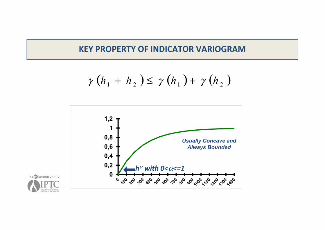
KEY PROPERTY OF INDICATOR VARIOGRAM

( ) ( ) ( )2121 hhhh γγγ +≤+

0,81

1,2

Usually Concave and

0,20,40,6

hα with 0<α< 1

Usually Concave and Always Bounded

00,2 hα with 0<α<=1

ARE THE STANDARD CONTINUOUS VARIOGRAM MODELS COMPATIBLE WITH INDICATOR VARIABLES?

1,4

1,6( ) ah

ah

ahCh ≤≤

−=γ 0

223

3

3?1

1,2

1,4

gram ( )

−=

−ah

eCh 1γ

( ) ahCh >=

γ ?0,4

0,6

0,8

Vario

g

SphericalExponentialGaussianCubic

( )

( )

−=

− 2

2

1 ah

eChγ

0

0,2

0 100 200 300 400 500 600 700 800 900 1000 1100 1200 1300 1400

Cubic

( ) ahah

ah

ah

ahCh ≤≤

−+−= 0

4

3

2

7

4

357 7

7

5

5

3

3

2

2γ

Distance ( ) ahCh >=

γ

WHAT IS LEFT?

1

1,2

0 6

0,8

1

ram Spherical

E ti l

0 2

0,4

0,6

Vario

gr Exponential

The spherical variogram has not been proved to be valid or invalid in 2D or 3D. But the exponential variogram has been

0

0,2 proved to be valid in all dimensions!

Distance

WHAT DO WE NEED?

1. Indicator Variogram Models that are Valid

2 Models allowing us to quantify probabilities of2. Models allowing us to quantify probabilities of Facies Transitions






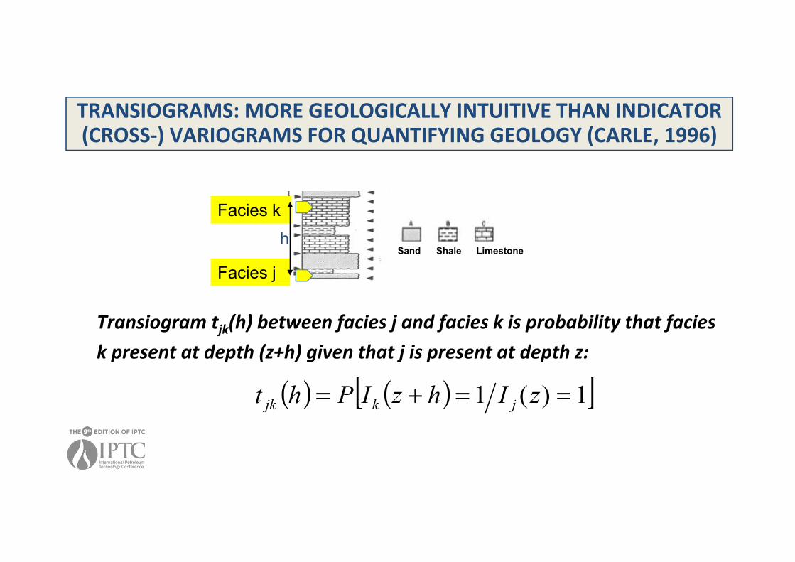
TRANSIOGRAMS: MORE GEOLOGICALLY INTUITIVE THAN INDICATOR (CROSS-) VARIOGRAMS FOR QUANTIFYING GEOLOGY (CARLE, 1996)

Facies k

Shale

Facies jSand Limestone

h

j

Transiogram tjk(h) between facies j and facies k is probability that faciesk d h ( h) i h j i d h

( ) ( )[ ]1)(1 ==+= zIhzIPht jkjk

k present at depth (z+h) given that j is present at depth z:

( ) ( )[ ]jkjk

EASIER TO OBTAIN AVERAGE SIZE OF BODIES FROM AUTO-TRANSIOGRAMS THAN FROM INDICATOR VARIOGRAMS(CARLE, 1996)

SILL Q(1-Q)( )htii

L1

( )ii

0L

pi

h0

AN EXAMPLE OF VERTICAL CROSS-TRANSIOGRAMS: ACCOUNTING FOR THE ARROW OF TIME! (CARLE, 1996)

QUANTIFYING ASYMMETRIES WITH EXPONENTIAL TRANSIOGRAMS MODELS

hhh λλλ hij

hij

hijjij eeepht 210

210)( λλλ βββ +++=

Nice but too limited!

ModelModel






TRUNCATED GAUSSIAN SIMULATION

facies #3facies #31Continuous

GaussianVariable

Simulation facies #1facies #1

0

1 facies #2facies #2

Simulation

FaciesIndicatorVariable

TRUNCATED GAUSSIANS AND WALTHER’S LAW: MODELLING DEPOSITIONAL ENVIRONMENTS ALONG A CARBONATE RAMP

Deep SubtidalSupratidal

Lower Intertidal

Shallow Subtidal

Upper Intertidal

TRUNCATED GAUSSIANS ALLOW THE CONSTRUCTION OF PERIODIC (HENCE NOT CONCAVE) INDICATOR VARIOGRAMS

1,400

1,000

1,200Variogram of continuous gaussian variable

0,400

0,600

0,800

Variogram of indicator variable after truncation

0,000

0,200

0 100 200 300 400 500 600 700 800 900 1000 1100 1200 1300 1400 1500

Variogram of indicator variable after truncation

G2 with spherical variogram

TRUNCATED PLURI-GAUSSIAN SIMULATIONS (PGS):USE TWO GAUSSIAN VARIABLES INSTEAD OF ONE!

2 continuous gaussianvariables simulations

p g

Facies simulationG1 with gaussian variogram

G2

G125% 25%

50%50%Truncation diagram

Allows more complex relationships between facies, and two anisotropies instead of one!

PLURI-GAUSSIAN SIMULATIONS (PGS): ALLOWS THE CONSTRUCTION OF MUCH MORE GENERAL VARIOGRAM OR TRANSIOGRAM MODELS






HYDROTHERMAL DOLOMITIZATION (LATEMAR PLATFORM, JACQUEMYN ET AL, 2014)

• Dolomite formation along permeable DOL• Dolomite formation along permeableconduits by subsurface Mg-bearing fluidwith temperature and pressure higher than

LST

DOL

of surrounding carbonate rocks.

HTD b di l t d l th d it

LST

• HTD bodies located along these conduits

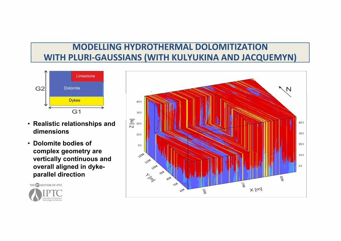
MODELLING HYDROTHERMAL DOLOMITIZATION WITH PLURI-GAUSSIANS (WITH KULYUKINA AND JACQUEMYN)

Limestone

Dolomite

Dykes

• Realistic relationships and dimensions

• Dolomite bodies of complex geometry are vertically continuous and overall aligned in dyke-parallel directionparallel direction

TRUNCATION DIAGRAM AND PGS REALIZATION, FLUVIAL ENVIRONMENT (DEBRIS FLOW AS CREVASSES)

Debris Flow

Channellood

plai

n

Levee ChannelF Levee

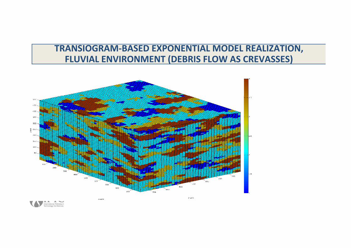
TRANSIOGRAM-BASED EXPONENTIAL MODEL REALIZATION, FLUVIAL ENVIRONMENT (DEBRIS FLOW AS CREVASSES)

Debris Floodplain Levee Channel

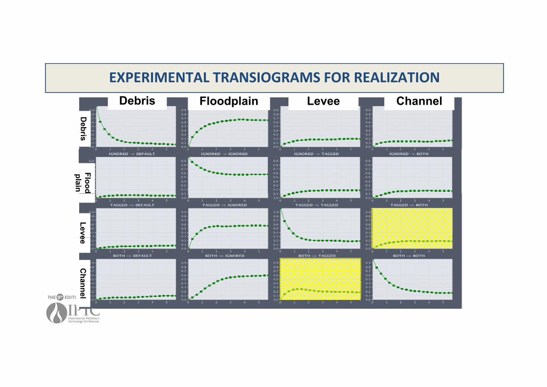
EXPERIMENTAL TRANSIOGRAMS FOR REALIZATIONp

Debris

Flood plain

LeveeeC

haannel

CONCLUSION

1. Variogram models valid for continuous variables are often not validfor Indicator Variables.

2. Exponential Transiograms valid in all dimensions and allowassymetries, but not flexible enough.

3. Truncated Gaussians mimic Walther’s Law for facies transitions.

4. Truncated Pluri-Gaussian approach allows the generation of more pp gflexible Transiograms.

5. Account for asymmetries and use more flexible models for modellingC b t R iCarbonate Reservoirs.

Slide 27

Acknowledgements / Thank You / Questions

Documents

Geostatistical Approaches for Quantifying Facies