Embed Size (px)
Citation preview

1
Data Mining amd Knowledge Acquisition
— Chapter 5 —
BIS 541
2012/2013 Spring

2
Chapter 7. Classification and Prediction
What is classification? What is prediction? Issues regarding classification and prediction Classification by decision tree induction Bayesian Classification Classification by Neural Networks Classification by Support Vector Machines (SVM) Classification based on concepts from association
rule mining Other Classification Methods Prediction Classification accuracy Summary
3
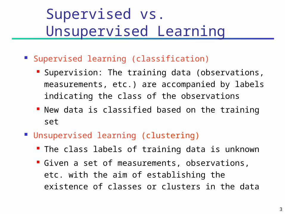
Supervised vs. Unsupervised Learning
Supervised learning (classification) Supervision: The training data (observations,
measurements, etc.) are accompanied by labels indicating the class of the observations
New data is classified based on the training set Unsupervised learning (clustering)
The class labels of training data is unknown Given a set of measurements, observations,
etc. with the aim of establishing the existence of classes or clusters in the data

44
Classification predicts categorical class labels (discrete or nominal) classifies data (constructs a model) based on the
training set and the values (class labels) in a classifying attribute and uses it in classifying new data
Numeric Prediction models continuous-valued functions, i.e., predicts
unknown or missing values Typical applications
Credit/loan approval: Medical diagnosis: if a tumor is cancerous or benign Fraud detection: if a transaction is fraudulent Web page categorization: which category it is
Prediction Problems: Classification vs. Numeric Prediction

5
Classification—A Two-Step Process
Model construction: describing a set of predetermined classes Each tuple/sample is assumed to belong to a predefined
class, as determined by the class label attribute The set of tuples used for model construction is training set The model is represented as classification rules, decision
trees, or mathematical formulae Model usage: for classifying future or unknown objects
Estimate accuracy of the model The known label of test sample is compared with the
classified result from the model Accuracy rate is the percentage of test set samples that
are correctly classified by the model Test set is independent of training set, otherwise over-
fitting will occur If the accuracy is acceptable, use the model to classify
data tuples whose class labels are not known

6
Classification Process (1): Model Construction
TrainingData
NAME RANK YEARS TENUREDMike Assistant Prof 3 noMary Assistant Prof 7 yesBill Professor 2 yesJim Associate Prof 7 yesDave Assistant Prof 6 noAnne Associate Prof 3 no
ClassificationAlgorithms
IF rank = ‘professor’OR years > 6THEN tenured = ‘yes’
Classifier(Model)
7
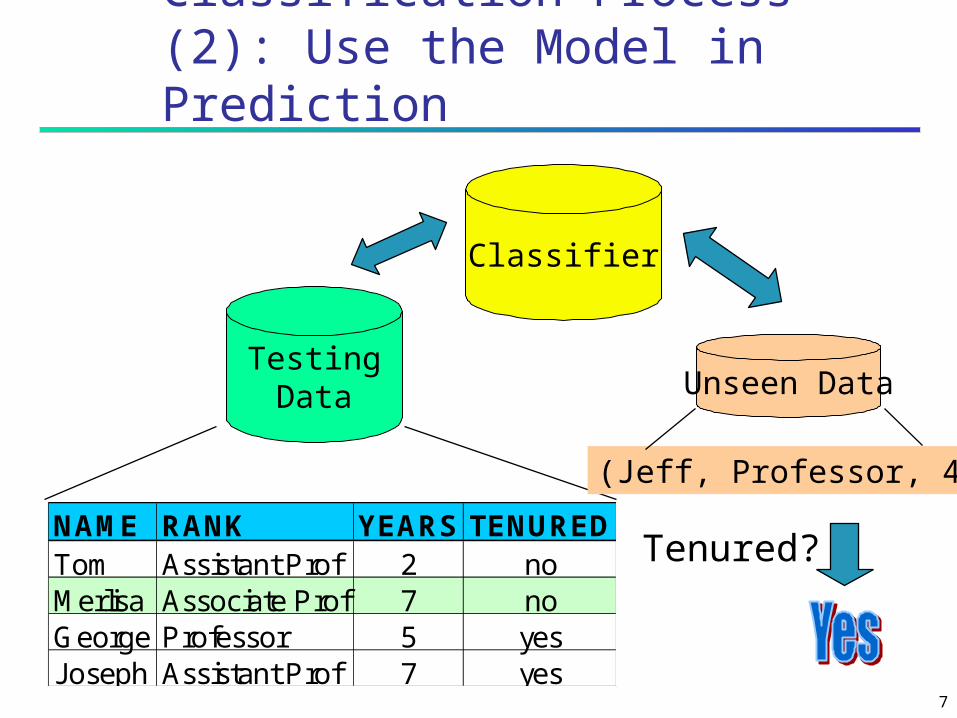
Classification Process (2): Use the Model in Prediction
Classifier
TestingData
NAME RANK YEARS TENUREDTom Assistant Prof 2 noMerlisa Associate Prof 7 noGeorge Professor 5 yesJoseph Assistant Prof 7 yes
Unseen Data
(Jeff, Professor, 4)
Tenured?

8
Chapter 7. Classification and Prediction
What is classification? What is prediction? Issues regarding classification and prediction Classification by decision tree induction Bayesian Classification Classification by Neural Networks Classification by Support Vector Machines (SVM) Classification based on concepts from association
rule mining Other Classification Methods Prediction Classification accuracy Summary

9
Issues Regarding Classification and Prediction (1): Data Preparation
Data cleaning Preprocess data in order to reduce noise and
handle missing values Relevance analysis (feature selection)
Remove the irrelevant or redundant attributes Data transformation
Generalize and/or normalize data

10
Issues regarding classification and prediction (2): Evaluating Classification Methods
Predictive accuracy Speed and scalability
time to construct the model time to use the model
Robustness handling noise and missing values
Scalability efficiency in disk-resident databases
Interpretability: understanding and insight provided by the model
Goodness of rules decision tree size compactness of classification rules

11
Chapter 7. Classification and Prediction
What is classification? What is prediction? Issues regarding classification and prediction Classification by decision tree induction Bayesian Classification Classification by Neural Networks Classification by Support Vector Machines (SVM) Classification based on concepts from association
rule mining Other Classification Methods Prediction Classification accuracy Summary
12
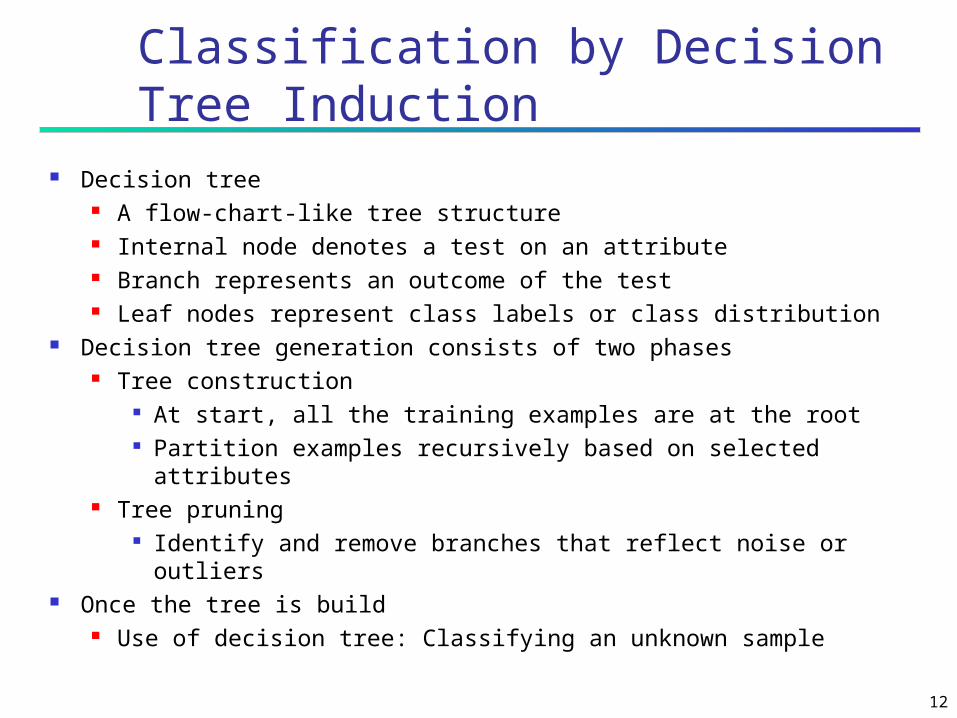
Classification by Decision Tree Induction
Decision tree A flow-chart-like tree structure Internal node denotes a test on an attribute Branch represents an outcome of the test Leaf nodes represent class labels or class distribution
Decision tree generation consists of two phases Tree construction
At start, all the training examples are at the root Partition examples recursively based on selected
attributes Tree pruning
Identify and remove branches that reflect noise or outliers Once the tree is build
Use of decision tree: Classifying an unknown sample

13
Training Dataset
age income student credit_rating buys_computer<=30 high no fair no<=30 high no excellent no31…40 high no fair yes>40 medium no fair yes>40 low yes fair yes>40 low yes excellent no31…40 low yes excellent yes<=30 medium no fair no<=30 low yes fair yes>40 medium yes fair yes<=30 medium yes excellent yes31…40 medium no excellent yes31…40 high yes fair yes>40 medium no excellent no
This follows an example from Quinlan’s ID3Han Table 7.1
Original data from DMPML Ch 4 Sec 4.3 pp 8-9,89-94
14
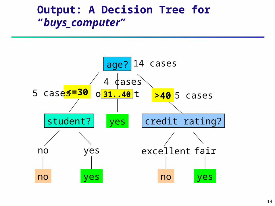
Output: A Decision Tree for “buys_computer”
age?
overcast
student? credit rating?
no yes fairexcellent
<=30 >40
no noyes yes
yes
31..40
14 cases
5 cases 5 cases
4 cases
15
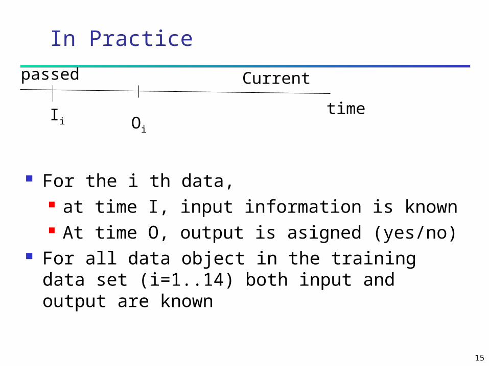
In Practice
For the i th data, at time I, input information is known At time O, output is asigned (yes/no)
For all data object in the training data set (i=1..14) both input and output are known
Ii Oi
passed Current
time

16
In Practice
For a new customers n, at the current time I, input information is known But O, output is not known
Yet to be classified as (yes or no) before its actual buying behavioris realized
Value of a data mining study to predict buying behavior beforehand
In On
passed Current
time
future

17
ID3 Algorithm for Decision Tree Induction
ID3 algorithm Quinlan (1986) Tree is constructed in a top-down recursive divide-and-
conquer manner At start, all the training examples are at the root Attributes are categorical (if continuous-valued, they are
discretized in advance) Examples are partitioned recursively based on selected
attributes Test attributes are selected on the basis of a heuristic or
statistical measure (e.g., information gain) Conditions for stopping partitioning
All samples for a given node belong to the same class There are no remaining attributes for further partitioning –
majority voting is employed for classifying the leaf There are no samples left

18
Entropy of a Simple Event
average amount of information to predict event s Expected information of an event s is
I(s)= -log2ps=log2(1/p) Ps is probability of event s entropy is high for lower probable events and
low otherwise as ps goes to zero
Event s becomes rare and rare and hence İts entropy approachs to infinity
as ps goes to one Event s becomes more and more certain and hence İts entropy approachs to zero
Hence entropy is a measure of randomness. disorder rareness of an event

19
10 0.50.25
1
2
entro
py
probability
Log21=0. log22=1Log20.5=log21/2=log22-1=-log22=-1Log20.25=-2Computational formulaLogax=logbx/logbaa and b any basisChoosing b as e It is more convenient tocompute logarithms of any basisLogax=logex/logeaor in particularLog2x=logex/loge2 orDropping e Log2x= lnx/ln2
Entropy=-log2p
Computational Formulas
20
Entropy of an simple event
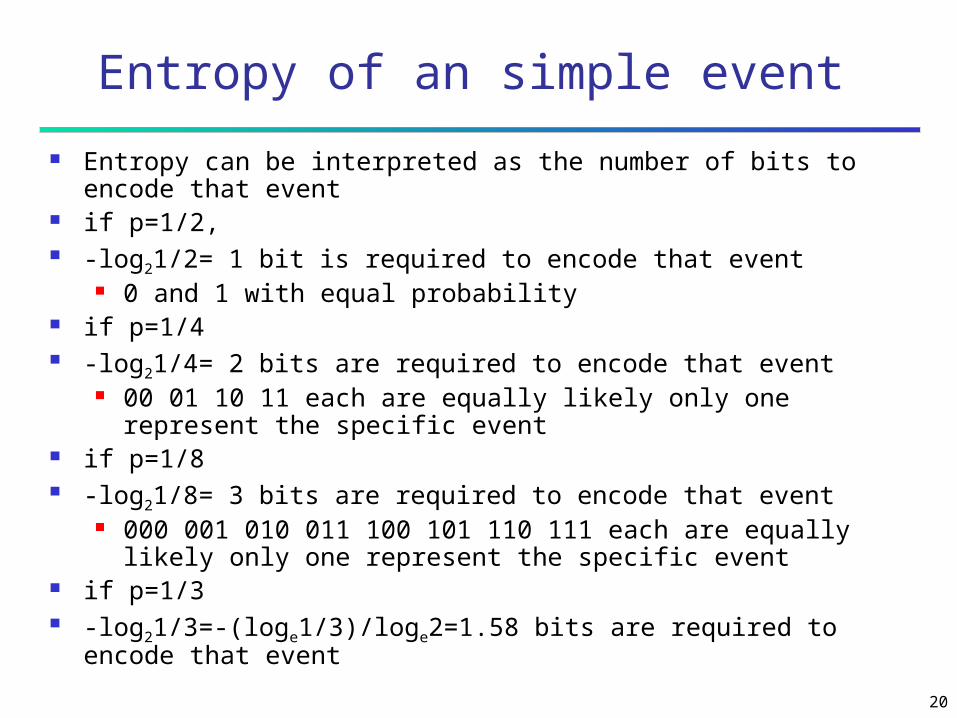
Entropy can be interpreted as the number of bits to encode that event
if p=1/2, -log21/2= 1 bit is required to encode that event
0 and 1 with equal probability if p=1/4 -log21/4= 2 bits are required to encode that event
00 01 10 11 each are equally likely only one represent the specific event
if p=1/8 -log21/8= 3 bits are required to encode that event
000 001 010 011 100 101 110 111 each are equally likely only one represent the specific event
if p=1/3 -log21/3=-(loge1/3)/loge2=1.58 bits are required to encode that
event
21
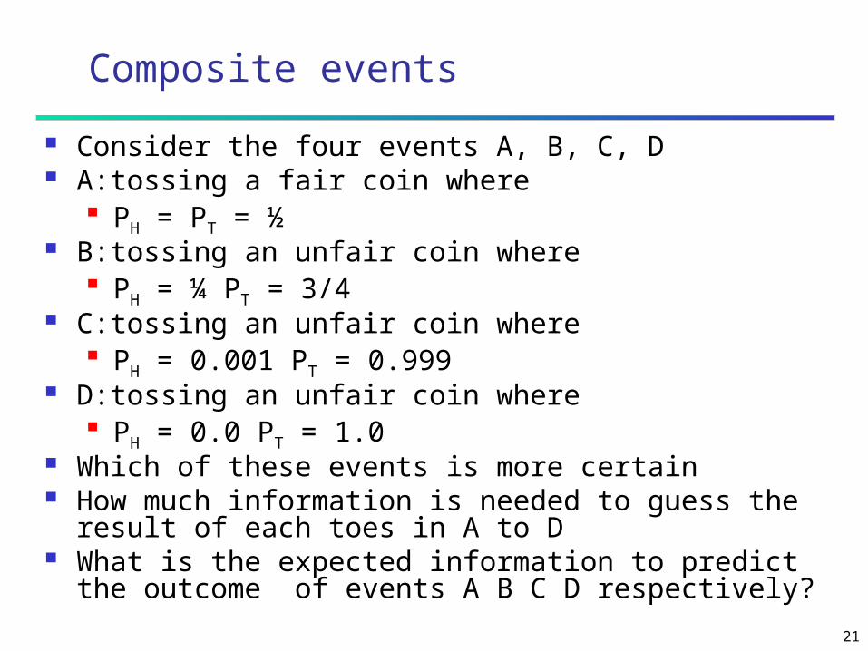
Composite events
Consider the four events A, B, C, D A:tossing a fair coin where
PH = PT = ½ B:tossing an unfair coin where
PH = ¼ PT = 3/4 C:tossing an unfair coin where
PH = 0.001 PT = 0.999 D:tossing an unfair coin where
PH = 0.0 PT = 1.0 Which of these events is more certain How much information is needed to guess the
result of each toes in A to D What is the expected information to predict the
outcome of events A B C D respectively?
22
Entropy of composite events
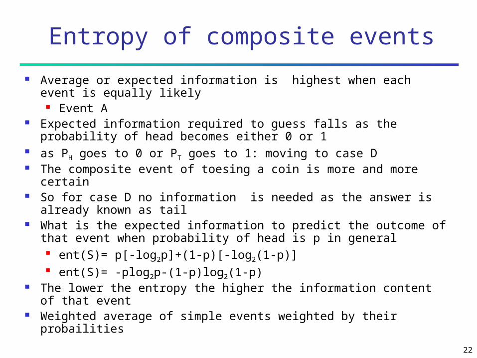
Average or expected information is highest when each event is equally likely
Event A Expected information required to guess falls as the probability
of head becomes either 0 or 1 as PH goes to 0 or PT goes to 1: moving to case D The composite event of toesing a coin is more and more certain So for case D no information is needed as the answer is
already known as tail What is the expected information to predict the outcome of that
event when probability of head is p in general ent(S)= p[-log2p]+(1-p)[-log2(1-p)] ent(S)= -plog2p-(1-p)log2(1-p)
The lower the entropy the higher the information content of that event
Weighted average of simple events weighted by their probailities

23
Examples
When the event is certain: pH = 1,pT= 0 or pH = 0, pT = 1 ent(S)= -1log2(1)-0log20= -1*0-0*log20=0
Note that: limx0+ xlog2x=0 For a fair coin pH = 0.5 ,pT= 0.5
ent(S)= -(1/2)log2(1/2)-(1/2)log21/2 = -1/2(-1) -1/2(-1)=1 Ent(S) is 1: p = 0.5 1-p=0.5
if head or tail probabilities are unequal entropy is between 0 and 1

24
0 1
Probability of head
Entropy= -plog2p-(1-p)log2(1-p)
1
0.5
P head versus entropy for the event of toesing a coin

25
In general
Entropy is a measure of (im)purity of an sample variable S is defined as
Ent(S) = sSps(-log2ps) = -sS pslog2ps
s is a value of S an element of sample space
ps is its estimated or subjective probability of any sS
Note that sps = 1
26
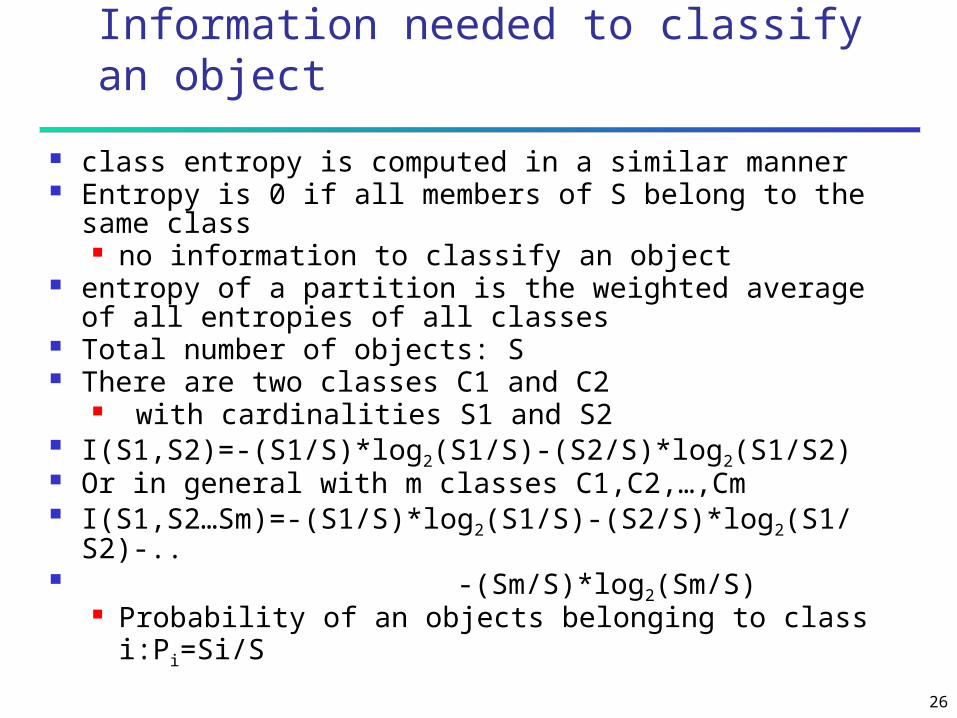
Information needed to classify an object
class entropy is computed in a similar manner Entropy is 0 if all members of S belong to the same
class no information to classify an object
entropy of a partition is the weighted average of all entropies of all classes
Total number of objects: S There are two classes C1 and C2
with cardinalities S1 and S2 I(S1,S2)=-(S1/S)*log2(S1/S)-(S2/S)*log2(S1/S2) Or in general with m classes C1,C2,…,Cm I(S1,S2…Sm)=-(S1/S)*log2(S1/S)-(S2/S)*log2(S1/S2)-.. -(Sm/S)*log2(Sm/S)
Probability of an objects belonging to class i:Pi=Si/S

27
Example cont.: At the root of the tree
There are 14 cases S = 14 9 yes denoted by Y, S1 = 9, py = 9/14 5 no denoted by N, S2 = 5, pn = 5/14
Y s and N s are almost equally likely How much information on the average is needed
to classify a person as buyer or not Without knowing any characteristics such as
age income … I(S1,S2)=(S1/S)(-log2S1/S) +(S2/S)(-log2S2/S) I(9,5)=(9/14)(-log29/14) + (5/14)(-log25/14) =(9/14)(0.637) + (5/14)(1.485) = 0.940 bits
of information close to 1

28
Expected information to classify with an attribute (1)
An attribute A with n distinct values as a1,a2,..,an partition the dataset into n distinct parts Si,j is number of objects in partition i (i=1..n) with a class Cj (j=1..m)
Expected information to classify an object knowing the value of attribute A is the weighted average of entropies of all
partitions Weighted by the frequency of that partition i

29
Expected information to classify with an attribute (2)
Ent(A) =I(A) = mj=1(ai/S) *I(Si,1..Si,m)
=(a1/S)*I(S1,1..S1,m)+(a2/S)*I(S2,1..S2,m)+… +(an/S)*I(Sn,1..Sn,m) I(Si,1..Si,m) entropy of any partition i I(Si,1..Si,m)=m
j=1(Sij/ai)(-log2Sij/ai) =-(Si1/ai)*log2Si1/ai-(Si2/ai)*log2Si2/ai-
...-(Sim/ai)*log2Sim/ai ai = m
j=1Sij = nuber of objects in each partition Here sij/ai is the probability of class j in partition i
30
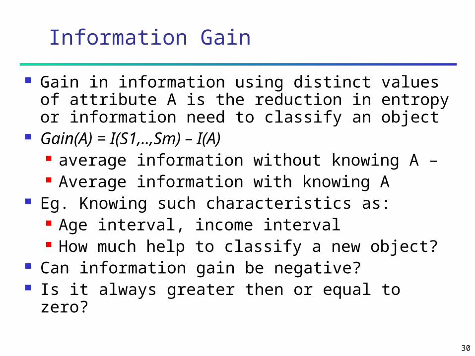
Information Gain
Gain in information using distinct values of attribute A is the reduction in entropy or information need to classify an object
Gain(A) = I(S1,..,Sm) – I(A) average information without knowing A – Average information with knowing A
Eg. Knowing such characteristics as: Age interval, income interval How much help to classify a new object?
Can information gain be negative? Is it always greater then or equal to zero?

31
Another Example
Pick up a student at random in BU What is the chance that she is staying in dorm?
Initially we have no specific information about her
If I ask initials Does it help us in predicting the probability of
her staying in dorm. No
If I ask her adress and record the city Does it help us in predcting the chance of her
staying in dorm Yes

32
Attribute selection at the root
There are four attributes age, income, student, credit rating
Which of these provıdes the highest informatıon in classıfying a new customer or equivalently
Which of these results in hıghest information gaın
33
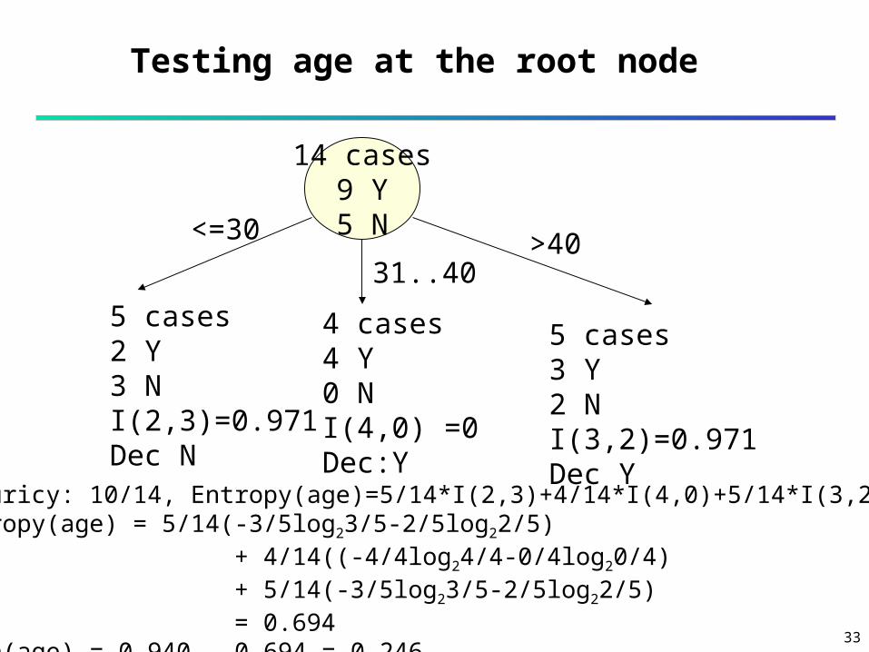
14 cases9 Y5 N
5 cases2 Y3 NI(2,3)=0.971Dec N
4 cases4 Y0 NI(4,0) =0Dec:Y
5 cases3 Y2 NI(3,2)=0.971 Dec Y
Accuricy: 10/14, Entropy(age)=5/14*I(2,3)+4/14*I(4,0)+5/14*I(3,2)Entropy(age) = 5/14(-3/5log23/5-2/5log22/5) + 4/14((-4/4log24/4-0/4log20/4) + 5/14(-3/5log23/5-2/5log22/5) = 0.694Gain(age) = 0.940 – 0.694 = 0.246
<=30
31..40>40
Testing age at the root node

34
Expected information for age <=30
If age is <=30 Information need to classify a new customer : I(2,3)=0.971 bits as the training data tells that Knowing that age <=30
with 0.4 probability a customer buys but with 0.6 probability she dose not
I(2,3)=-(3/5)log23/5-(2/5)log22/5= 0.971 = 0.6*0.734 + 0.4*1.322 = 0.971 But what is the weight of age range <=30 5 out of 14 samples are in that range (5/14)*I(2,3) is the weighted information need to
classify a customer as buyer or not

35
Information gain by age
gain(age)= I(Y,N)-Entropy(age) = 0.940 – 0.694 =0.246 is the information gain Or reduction of entropy to classify a new
object Knowing the age of the customer increases
our ability to classify her as buyer or not or Help us to predict her buying behavior

36
Attribute Selection by Information Gain Computation
Class Y: buys_computer = “yes”
Class N: buys_computer = “no” I(Y, N) = I(9, 5) =0.940 Compute the entropy for age:
means “age <=30” has
5 out of 14 samples, with 2
yes’es and 3 no’s. Hence
Similarly,
age Yi Ni I(pi, ni)<=30 2 3 0.97130…40 4 0 0>40 3 2 0.971
694.0)2,3(14
5
)0,4(14
4)3,2(
14
5)(
I
IIageE
048.0)_(
151.0)(
029.0)(
ratingcreditGain
studentGain
incomeGain
246.0)(),()( ageENYIageGainage income student credit_rating buys_computer<=30 high no fair no<=30 high no excellent no31…40 high no fair yes>40 medium no fair yes>40 low yes fair yes>40 low yes excellent no31…40 low yes excellent yes<=30 medium no fair no<=30 low yes fair yes>40 medium yes fair yes<=30 medium yes excellent yes31…40 medium no excellent yes31…40 high yes fair yes>40 medium no excellent no
)3,2(14
5I
37
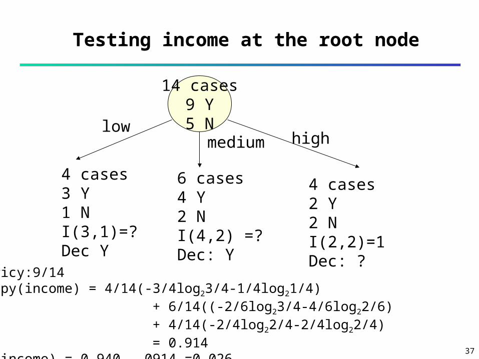
14 cases9 Y5 N
4 cases3 Y1 NI(3,1)=? Dec Y
6 cases4 Y 2 NI(4,2) =?Dec: Y
4 cases2 Y2 NI(2,2)=1Dec: ?
Accuricy:9/14Entropy(income) = 4/14(-3/4log23/4-1/4log21/4) + 6/14((-2/6log23/4-4/6log22/6) + 4/14(-2/4log22/4-2/4log22/4) = 0.914Gain(income) = 0.940 – 0914.=0.026
lowmedium high
Testing income at the root node
38
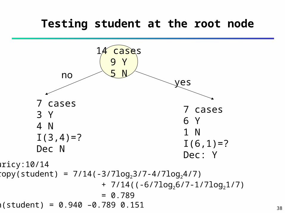
14 cases9 Y5 N
7 cases3 Y4 NI(3,4)=? Dec N
7 cases6 Y1 NI(6,1)=?Dec: Y
Accuricy:10/14Entropy(student) = 7/14(-3/7log23/7-4/7log24/7) + 7/14((-6/7log26/7-1/7log21/7) = 0.789Gain(student) = 0.940 –0.789 0.151
noyes
Testing student at the root node

39
14 cases9 Y5 N
8 cases6 Y2 NI(6,2)=? Dec Y
6 cases3 Y3 NI(3,3)=1Dec: ?
Accuricy:9/14Entropy(student) = 8/14(-2/6log22/6-4/6log24/6)+ + 6/14((-3/6log23/6-3/6log23/6) = 0.892Gain(credit rating) = 0.940 – 0892=0.048
faırexcellent
Testing credit rating at the root node

40
Comparıng gaıns
İnformation gains for attrıbutes at the root node:
Gain(age) = 0.246 Gain(age) = 0.026 Gain(age) = 0.151 Gain(age) = 0.048 Age provıdes the highest gain in information Age ıs choosen as the attribute at the root
node Branch acording to the distinct values of age

41
After Selecting age first level of the tree
age?
overcast
Continue continue
<=30 >40
yes
31..40
14 cases
5 cases 5 cases
4 cases
42
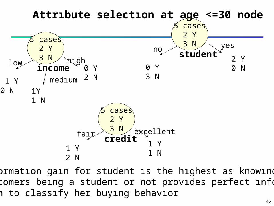
5 cases2 Y3 N
1 Y0 N 1Y
1 N
low hıghincome
5 cases2 Y3 N
0 Y3 N
2 Y 0 N
no yesstudent
5 cases2 Y3 N
1 Y2 N
1 Y1 N
faır excellentcredit
Attrıbute selectıon at age <=30 node
0 Y2 Nmedıum
Informatıon gaın for student ıs the hıghest as knowıng the Customers beıng a student or not provıdes perfect ınforma-tıon to classıfy her buyıng behavıor

43
5 cases3 Y2 N
1 Y1 N 2Y
1 N
low hıghincome
5 cases3 Y2 N
1 Y1 N
2 Y1 N
no yesstudent
5 cases3 Y2 N
3 Y0 N
0 Y2 N
faır excellentcredit
Attrıbute selectıon at age >40 node
0 Y0 Nmedıum
Informatıon gaın for credıt ratıng ıs the hıghest as knowıng the Customers beıng a student or not provıdes perfect ınforma-tıon to classıfy her buyıng behavıor

44
Exercise
Calculate all information gains in the second level of the tree that is after branching by the distinct values of age
45
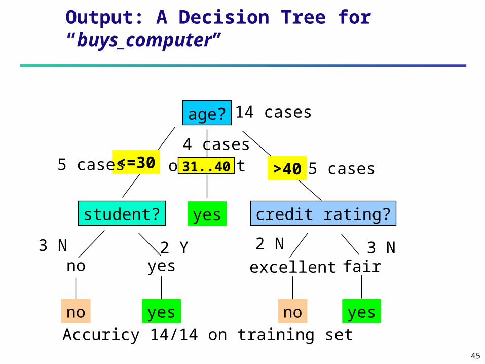
Output: A Decision Tree for “buys_computer”
age?
overcast
student? credit rating?
no yes fairexcellent
<=30 >40
no noyes yes
yes
31..40
14 cases
5 cases 5 cases
4 cases
3 N 3 N2 N 2 Y
Accuricy 14/14 on training set
46
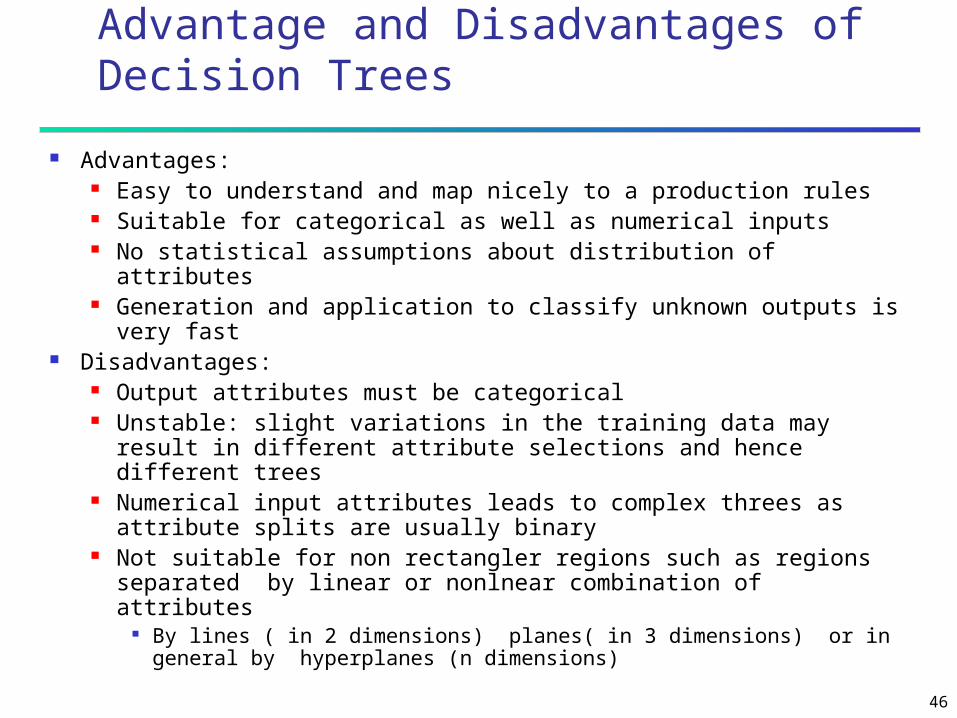
Advantage and Disadvantages of Decision Trees
Advantages: Easy to understand and map nicely to a production rules Suitable for categorical as well as numerical inputs No statistical assumptions about distribution of attributes Generation and application to classify unknown outputs is
very fast Disadvantages:
Output attributes must be categorical Unstable: slight variations in the training data may result
in different attribute selections and hence different trees Numerical input attributes leads to complex threes as
attribute splits are usually binary Not suitable for non rectangler regions such as regions
separated by linear or nonlnear combination of attributes By lines ( in 2 dimensions) planes( in 3 dimensions) or in
general by hyperplanes (n dimensions)

47
age
income
x
xx
x
x
xxx
x
o
oo
oo o o
The two classes X and Oare separated by line AA
Decision trees are not suitabe For this problem
A
A
A classification problem in that decision trees are not suitable to classify

48
Other Attribute Selection Measures
Gain Ratio Gini index (CART, IBM IntelligentMiner)
All attributes are assumed continuous-valued Assume there exist several possible split
values for each attribute May need other tools, such as clustering, to
get the possible split values Can be modified for categorical attributes

49
Gain Ratio
Add another attribute transaction TID for each observation TID is different E(TID)= (1/14)*I(1,0)+(1/14)*I(1,0)+ (1/14)*I(1,0)...
+ (1/14)*I(1,0)=0 gain(TID)= 0.940-0=0.940 the highest gain so TID is the test attribute
which makes no sense use gain ratio rather then gain Split information: measure of the information value
of split: without considering class information only number and size of child nodes A kind of normalization for information gain

50
Split information = (-Si/S)log2(Si/S) information needed to assign an instance to one
of these branches Gain ratio = gain(S)/split information(S) in the previous example Split info and gain ratio for TID:
split info(TID) = [(1/14)log2(1/14)]*14=3.807 gain ratio(TID) = (0.940-0.0)/3.807=0.246
Split info for age:I(5,4,5)= (5/14)log25/14+ (4/14)log24/14
+(5/14)log25/14=1.577 gain ratio(age) = gain(age)/split info(age)
= 0.247/1.577=0.156
51
Gini Index (IBM IntelligentMiner)
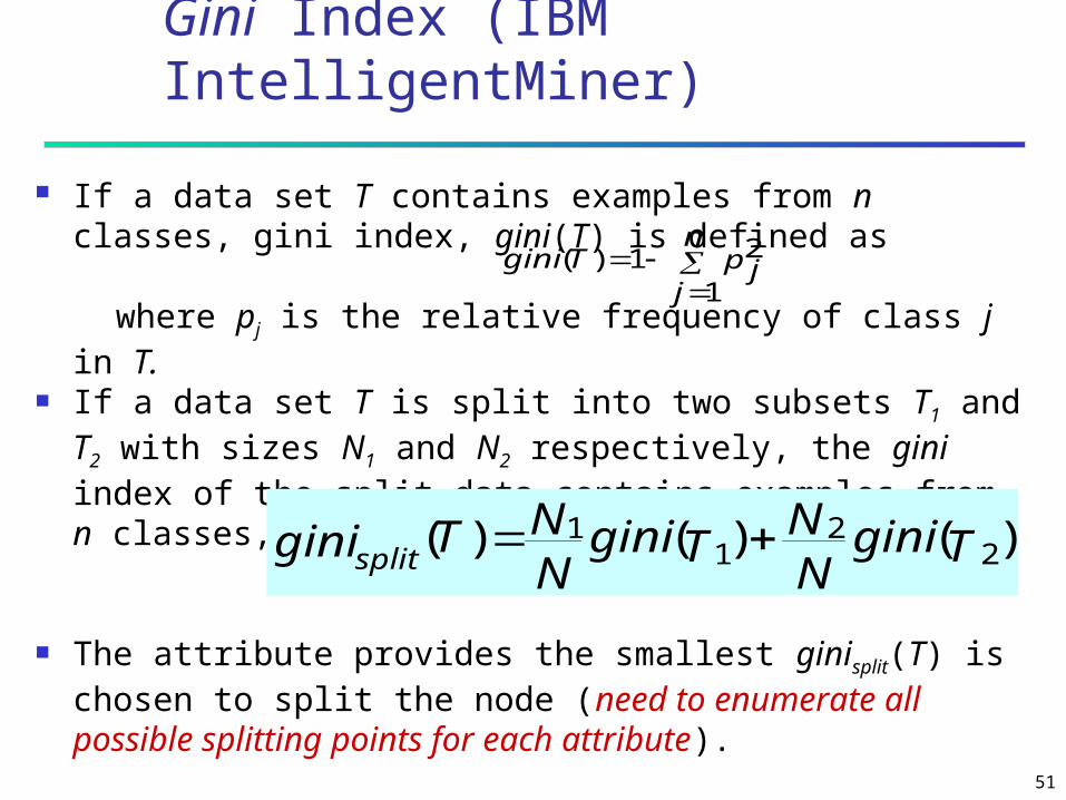
If a data set T contains examples from n classes, gini index, gini(T) is defined as
where pj is the relative frequency of class j in T. If a data set T is split into two subsets T1 and T2 with
sizes N1 and N2 respectively, the gini index of the split data contains examples from n classes, the gini index gini(T) is defined as
The attribute provides the smallest ginisplit(T) is chosen to split the node (need to enumerate all possible splitting points for each attribute).
n
jp jTgini
1
21)(
)()()( 22
11 Tgini
NN
TginiNNTginisplit

52
Gini index (CART) Example
Ex. D has 9 tuples in buys_computer = “yes” and 5 in “no”
Suppose the attribute income partitions D into 10 in D1: {low,
medium} and 4 in D2
but gini{medium,high} is 0.30 and thus the best since it is the
lowest D1:{medium,high}, D2:{low} gini index: 0.300 D1:{low,high}, D2:{medium} gini index: 0.315 Highest gini is for D1:{low,medium}, D2:{high}
459.014
5
14
91)(
22
Dgini
)(14
4)(
14
10)( 11},{ DGiniDGiniDgini mediumlowincome
53
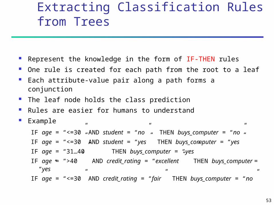
Extracting Classification Rules from Trees
Represent the knowledge in the form of IF-THEN rules One rule is created for each path from the root to a leaf Each attribute-value pair along a path forms a conjunction The leaf node holds the class prediction Rules are easier for humans to understand Example
IF age = “<=30” AND student = “no” THEN buys_computer = “no”
IF age = “<=30” AND student = “yes” THEN buys_computer = “yes”
IF age = “31…40” THEN buys_computer = “yes”
IF age = “>40” AND credit_rating = “excellent” THEN buys_computer = “yes”
IF age = “<=30” AND credit_rating = “fair” THEN buys_computer = “no”

54
Approaches to Determine the Final Tree Size
Separate training (2/3) and testing (1/3) sets Use cross validation, e.g., 10-fold cross
validation Use all the data for training
but apply a statistical test (e.g., chi-square) to estimate whether expanding or pruning a node may improve the entire distribution
Use minimum description length (MDL) principle halting growth of the tree when the encoding
is minimized
55
Enhancements to basic decision tree induction
Allow for continuous-valued attributes Dynamically define new discrete-valued attributes
that partition the continuous attribute value into a discrete set of intervals
Handle missing attribute values Assign the most common value of the attribute Assign probability to each of the possible values
Attribute construction Create new attributes based on existing ones that
are sparsely represented This reduces fragmentation, repetition, and
replication

56
Avoid Overfitting in Classification
Overfitting: An induced tree may overfit the training data Too many branches, some may reflect anomalies
due to noise or outliers Poor accuracy for unseen samples
Two approaches to avoid overfitting Prepruning: Halt tree construction early—do not
split a node if this would result in the goodness measure falling below a threshold
Difficult to choose an appropriate threshold Postpruning: Remove branches from a “fully grown”
tree—get a sequence of progressively pruned trees Use a set of data different from the training data
to decide which is the “best pruned tree”

57
If the error rate of a subtree is higher then the error obtained by replacing the tree with its most frequent leaf or branch prune the subtree
How to estimate the prediction error do not use training samples
pruning always increase error of the training sample
estimate error based on test set cost complexity or reduced error pruning

58
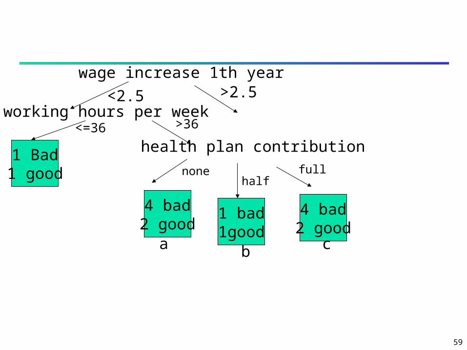
Example
Labour negotiation data dependent variable or class to be
predicted: acceptability of contract: good or bad
independent variables: duration, wage increase 1th year: <%2.5, >%2.5 working hours per week: <36, >36 health plan contribution: none, half, full
Figure 6.2 WF shows a branch of a d.tree
59
wage increase 1th year
<2.5 >2.5working hours per week
1 Bad1 good
health plan contribution
4 bad2 good
1 bad1good
4 bad2 good
<=36 >36
nonehalf
full
a b c

60
AnswerTree
Variables measurement levels case weights frequency variables
Growing methods Stopping rules Tree parameters
costs, prior probabilities, scores and profits Gain summary Accuracy of tree Cost-complexity pruning
61
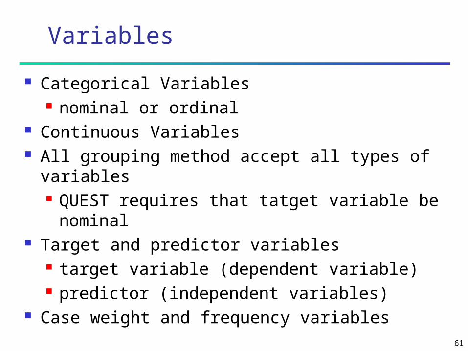
Variables
Categorical Variables nominal or ordinal
Continuous Variables All grouping method accept all types of
variables QUEST requires that tatget variable be
nominal Target and predictor variables
target variable (dependent variable) predictor (independent variables)
Case weight and frequency variables
62
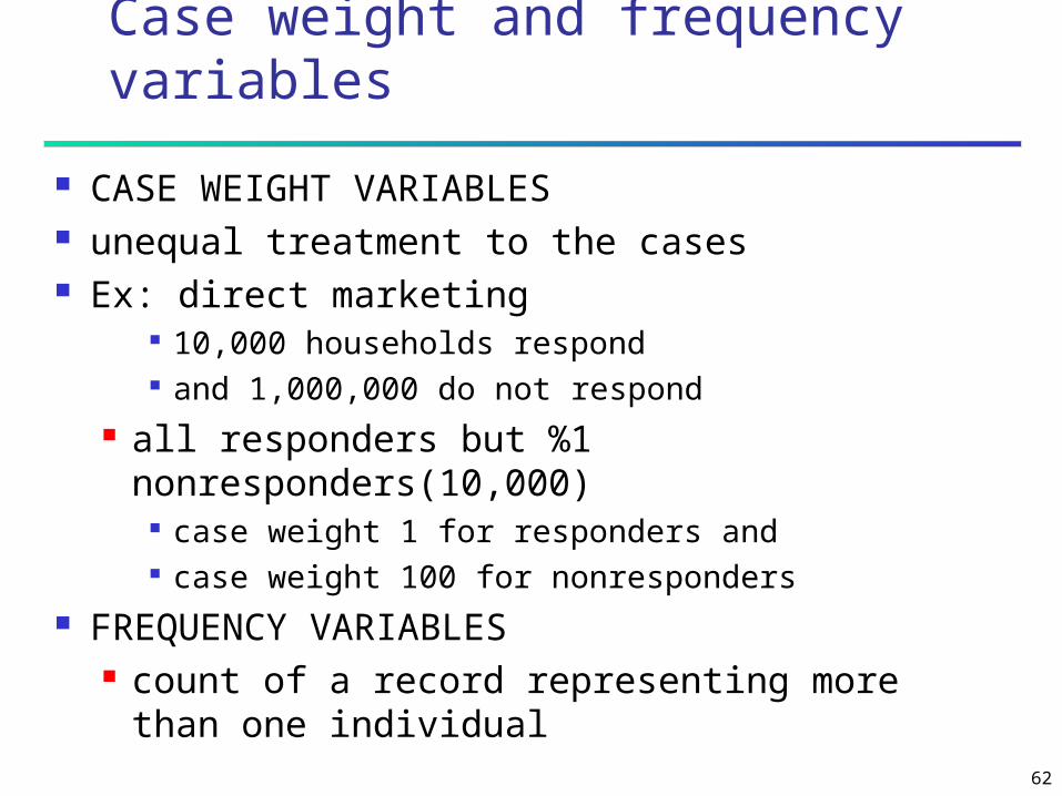
Case weight and frequency variables
CASE WEIGHT VARIABLES unequal treatment to the cases Ex: direct marketing
10,000 households respond and 1,000,000 do not respond
all responders but %1 nonresponders(10,000)
case weight 1 for responders and case weight 100 for nonresponders
FREQUENCY VARIABLES count of a record representing more than one
individual
63
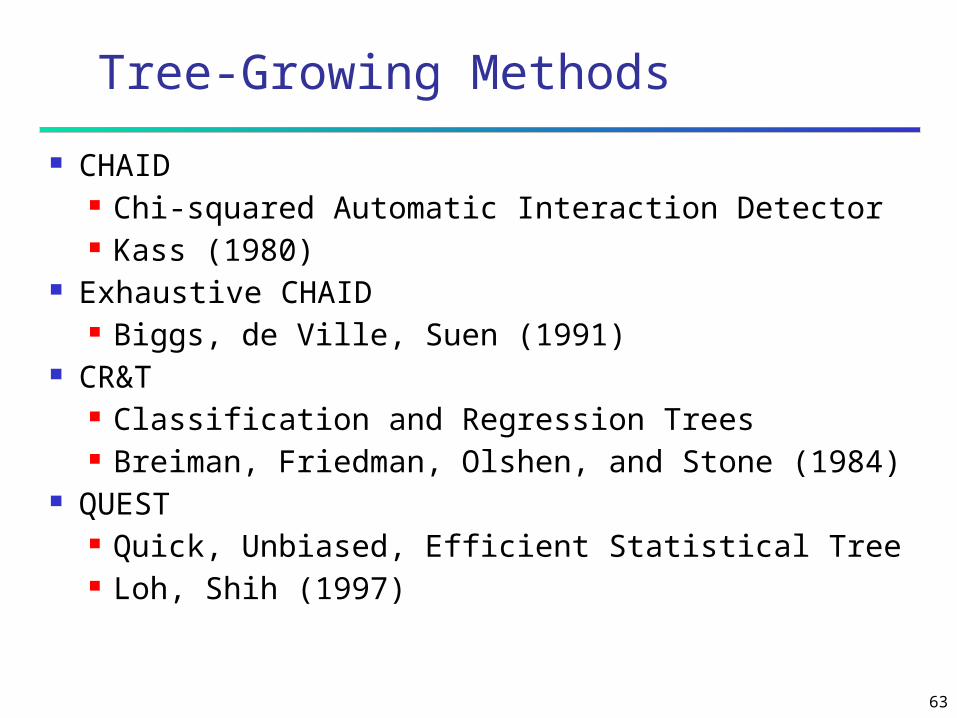
Tree-Growing Methods
CHAID Chi-squared Automatic Interaction Detector Kass (1980)
Exhaustive CHAID Biggs, de Ville, Suen (1991)
CR&T Classification and Regression Trees Breiman, Friedman, Olshen, and Stone (1984)
QUEST Quick, Unbiased, Efficient Statistical Tree Loh, Shih (1997)

64
CHAID
evaluate all values of a potential predictor merges values that are judged to be
statistically homogenous target variable
continuous F test categorical Chi-square test
not binary: produce more than two categories at any particular level wider tree than do the binary methods works for all types of variables case weights and frequency variables missing values as a single valid category
65
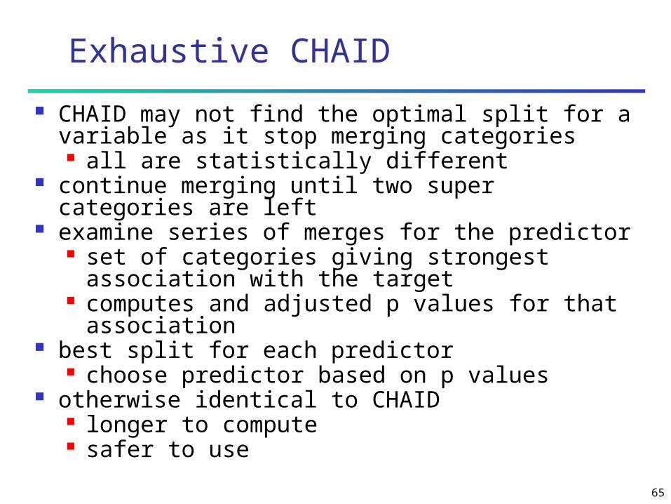
Exhaustive CHAID
CHAID may not find the optimal split for a variable as it stop merging categories all are statistically different
continue merging until two super categories are left
examine series of merges for the predictor set of categories giving strongest
association with the target computes and adjusted p values for that
association best split for each predictor
choose predictor based on p values otherwise identical to CHAID
longer to compute safer to use
66
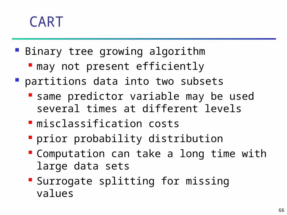
CART
Binary tree growing algorithm may not present efficiently
partitions data into two subsets same predictor variable may be used
several times at different levels misclassification costs prior probability distribution Computation can take a long time with
large data sets Surrogate splitting for missing values
67
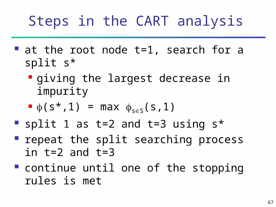
Steps in the CART analysis
at the root node t=1, search for a split s* giving the largest decrease in impurity (s*,1) = max sS(s,1)
split 1 as t=2 and t=3 using s* repeat the split searching process in t=2
and t=3 continue until one of the stopping rules is
met

68
Stoping rules
all cases have identical values for all predictors the node becomes pure; all cases have the
same value of the target variable the depth of the tree has reached its
prespecified maximum value the number of cases in a node less than a
prespecified minimum parent node size split at node results in producing a child node
with cases less than a prespecified min child node size
for CART only: max decrease in impurity is less than a prespecified value
69
QUEST
variable selection and split point selection separately
computationally efficient than CART

70
Classification in Large Databases
Classification—a classical problem extensively studied by statisticians and machine learning researchers
Scalability: Classifying data sets with millions of examples and hundreds of attributes with reasonable speed
Why decision tree induction in data mining? relatively faster learning speed (than other
classification methods) convertible to simple and easy to understand
classification rules can use SQL queries for accessing databases comparable classification accuracy with other methods
71
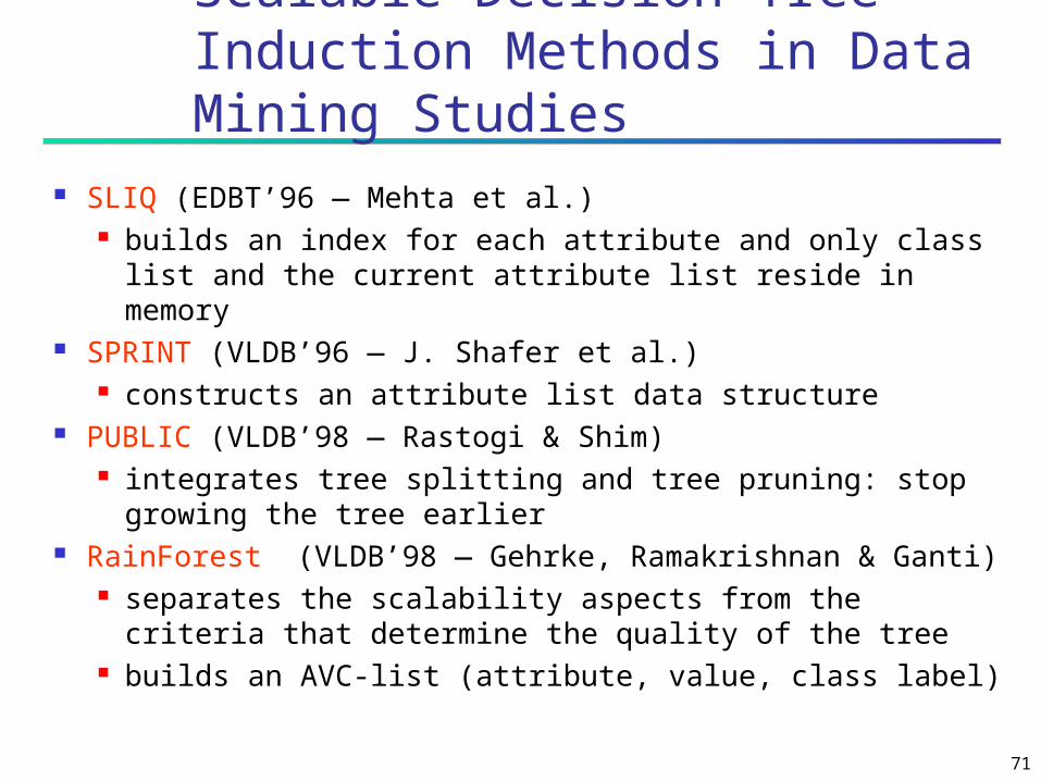
Scalable Decision Tree Induction Methods in Data Mining Studies
SLIQ (EDBT’96 — Mehta et al.) builds an index for each attribute and only class list
and the current attribute list reside in memory SPRINT (VLDB’96 — J. Shafer et al.)
constructs an attribute list data structure PUBLIC (VLDB’98 — Rastogi & Shim)
integrates tree splitting and tree pruning: stop growing the tree earlier
RainForest (VLDB’98 — Gehrke, Ramakrishnan & Ganti) separates the scalability aspects from the criteria
that determine the quality of the tree builds an AVC-list (attribute, value, class label)