Embed Size (px)
Citation preview

1
Beyond 5G with UAVs: Foundations of a 3D
Wireless Cellular NetworkMohammad Mozaffari1, Ali Taleb Zadeh Kasgari2, Walid Saad2, Mehdi Bennis3,
and Merouane Debbah4
1 Ericsson Research, Santa Clara, CA, USA, Email: [email protected] Wireless@VT, Electrical and Computer Engineering Department, Virginia Tech, VA, USA,
Emails:alitk,[email protected] CWC - Centre for Wireless Communications, University of Oulu, Finland, Email: [email protected].
4 Mathematical and Algorithmic Sciences Lab, Huawei France R & D, Paris, France, and CentraleSupelec,
Universite Paris-Saclay, Gif-sur-Yvette, France, Email: [email protected].
Abstract
In this paper, a novel concept of three-dimensional (3D) cellular networks, that integrate drone base
stations (drone-BS) and cellular-connected drone users (drone-UEs), is introduced. For this new 3D
cellular architecture, a novel framework for network planning for drone-BSs as well as latency-minimal
cell association for drone-UEs is proposed. For network planning, a tractable method for drone-BSs’
deployment based on the notion of truncated octahedron shapes is proposed that ensures full coverage
for a given space with minimum number of drone-BSs. In addition, to characterize frequency planning
in such 3D wireless networks, an analytical expression for the feasible integer frequency reuse factors
is derived. Subsequently, an optimal 3D cell association scheme is developed for which the drone-UEs’
latency, considering transmission, computation, and backhaul delays, is minimized. To this end, first,
the spatial distribution of the drone-UEs is estimated using a kernel density estimation method, and the
parameters of the estimator are obtained using a cross-validation method. Then, according to the spatial
distribution of drone-UEs and the locations of drone-BSs, the latency-minimal 3D cell association for
drone-UEs is derived by exploiting tools from optimal transport theory. Simulation results show that the
proposed approach reduces the latency of drone-UEs compared to the classical cell association approach
that uses a signal-to-interference-plus-noise ratio (SINR) criterion. In particular, the proposed approach
yields a reduction of up to 46% in the average latency compared to the SINR-based association. The
A preliminary conference version of this work appears in [1].
Mohammad Mozaffari joined Ericsson in July 2018. He was with Wireless@VT, Electrical and Computer Engineering
Department, Virginia Tech, VA, USA, when this work was done.
arX
iv:1
805.
0653
2v2
[cs
.IT
] 2
Nov
201
8
2
results also show that the proposed latency-optimal cell association improves the spectral efficiency of
a 3D wireless cellular network of drones.
I. INTRODUCTION
Recent reports from the federal aviation administration (FAA) shows that the number of
unmanned aerial vehicles (UAVs), also known as drones, will exceed 7 million in 2020 [2]. Such
a massive use of drones will have significant impacts on wireless networking. From a wireless
perspective, the two key roles of drones include: aerial base station (BS), and user equipment
(UE) [3]–[5]. Due to their flexibility and inherent ability for line-of-sight (LoS) communications,
drone-BSs can provide broadband, wide-scale, and reliable wireless connectivity during disasters
and temporary events [4]–[11]. Moreover, drone-BSs offer a promising solution for ultra-flexible
deployment and cost-effective wireless services, without the prohibitive costs of terrestrial BSs.
Meanwhile, drones can also act as UEs (i.e., cellular-connected drone-UEs) that must connect
to a wireless network so as to operate. In particular, cellular-connected drone-UEs can be used for
wide range of applications such as package delivery [12], surveillance, remote sensing, and virtual
reality. The key feature of drone-UEs is their ability to intelligently move in three dimensions
and optimize their trajectory in order to efficiently complete their missions. Therefore, drone-
UEs are widely used for delivery purposes such as in Amazon’s prime air drone delivery service
and drug delivery in medical applications.
Wireless networking with drones faces a number of challenges. For instance, for drone-
BSs, key design problems include 3D deployment and network planning, performance analysis,
resource allocation, and cell association. For drone-UEs, there is a need for reliable and low
latency communications for efficient control. However, existing terrestrial cellular networks
have been primarily designed for supporting ground users and are not able to readily serve
aerial users. In fact, terrestrial BSs may not be able to meet the low-latency and reliable
communication requirements of drone-UEs due to blockage effects and the specific design of the
BSs’ antennas which are not suitable for supporting users at high-elevation angles. Also, in areas
with geographical constraints, terrestrial BSs may not be available to provide wireless service
to drone-UEs. In such cases, the deployment of aerial drone-BSs is a promising opportunity for
providing reliable wireless connectivity for drone-UEs. Clearly, to support drones in wireless

3
networking applications, there is a need for developing the novel concept of a 3D cellular
network that incorporates both drone-BSs and drone-UEs.
A. Related Works on Drone Communications
Recent studies on drone communications have investigated various design challenges that
include performance characterization, trajectory optimization, 3D deployment, user-to-drone as-
sociation, and cellular-connected UAVs. For instance, in [7], the authors proposed an algorithm
for jointly optimizing the locations and number of drones to maximize wireless coverage. The
work in [13] studied the optimal 3D deployment of UAVs for maximizing the number of
covered ground users under quality-of-service (QoS) constraints. In [14], the authors proposed a
framework for strategic placement of multiple drone-BSs that provides wireless connectivity for
a large-scale ground network. However, the prior studies on deployment of UAV base stations
ignore the existence of flying drone-UEs.
In addition, the work in [15] presented a delay-optimal cell association scheme in a UAV-
assisted terrestrial wireless network. The work in [16] studied the optimal user-UAV association
for capacity improvement in UAV-enabled heterogeneous wireless networks. The work in [17]
proposed a novel hybrid network architecture for cellular systems by using UAVs as aerial base
stations for data offloading. In particular, with the proposed framework in [17], the minimum
throughput of mobile terminals is maximized by jointly optimizing the user partitioning, the
spectrum allocation, as well as the UAV trajectory. In [18], the authors proposed an algorithm for
maximizing the sum-rate of ground users by joint optimization of user-to-drone-BSs association
and wireless backhaul bandwidth allocation. The work in [19] proposed a novel cell association
approach that maximizes the total data delivered to ground users by drone-BSs that have limited
flight endurance. However, the previous works on user association in drone networks are limited
to ground users and do not consider 3D aerial users. Moreover, the previous works do not analyze
latency (due to e.g., communication, computation, and backhaul) which is a key metric in 3D
drone communication systems.
While there exists a number of studies on cellular-connected drone-UEs [20]–[22], the po-
tential use of drone-BSs for serving drone-UEs has not been considered. For example, in [20],
the authors studied the coexistence of drone-UEs and ground users in cellular networks and
characterized the downlink coverage performance. The work in [21] proposed an interference-

4
aware path planning approach for drone-UEs with the goal of minimizing their communication
latency and their interference on terrestrial users. In [23], the authors analyzed the downlink
coverage performance of drone-UEs that communicate with terrestrial base stations. In [22], the
authors proposed a trajectory design scheme for minimizing the mission time of a single UAV-UE.
Meanwhile, the authors in [24] characterized the performance of drone-UEs in uplink commu-
nications with ground BSs in terms of blocking probability and average achievable throughput.
However, the existing studies on cellular-connected UAVs do not exploit the deployment of aerial
base stations for enabling low-latency and reliable drone-UEs’ communications.
However, none of these previous works [4]–[8], [13]–[16], [18]–[22], [25], studied a 3D
wireless network of co-existing aerial base stations and users (i.e., drone-BSs and drone-UEs)
while addressing network planning, deployment, and latency-aware cell association problems.
B. Contributions
The main contribution of this paper is to introduce the novel concept of a fully-fledged drone-
based 3D cellular network that incorporates drone-UEs, low-altitude platform (LAP) drone-
BSs, and high-altitude platform (HAP) drones. In this new 3D cellular network architecture, we
propose a framework for addressing the two fundamental problems of network planning and 3D
cell association. In particular, our proposed framework includes a tractable approach for three-
dimensional placement and frequency planning for drone-BSs, as well as a latency-minimal 3D
cell association scheme for servicing drone-UEs. For deployment, we introduce a new approach
based on truncated octahedron cells that determines the minimum number of drone-BSs that can
cover a 3D space, along with their locations. Furthermore, for frequency planning in the proposed
3D wireless network, we derive an analytical expression for the feasible integer frequency reuse
factors. To perform latency-minimal 3D cell association, first, we estimate the spatial distribution
of drone-UEs by using a kernel density estimation method. Then, given the locations of drone-
BSs and the distribution of drone-UEs, we find the optimal 3D cell association for which the
total latency of serving drone-UEs is minimized. In this case, we analytically characterize the
optimal 3D cell partitions by exploiting tools from optimal transport theory. Our results show
that the proposed approach significantly reduces the latency of serving drone-UEs, compared
to classical cell association approach that uses signal-to-interference-plus-noise ratio (SINR)
criterion. In particular, our approach yields around 46% reduction in the average total latency
5
Drone-BS
Drone-UE
HAP drone
3D cell association
Drone-BS n
3D spatial distribution of
Drone-UEs
Backhaul link
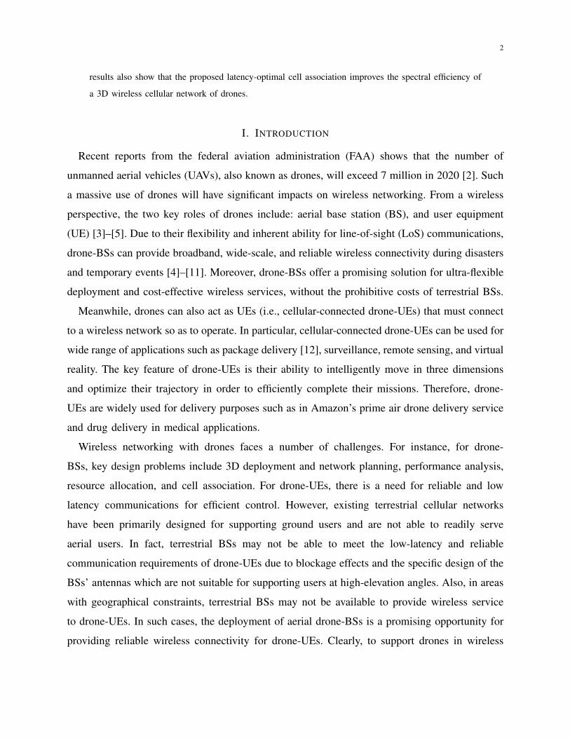
Fig. 1: The proposed 3D wireless network with drone-BSs, drone-UEs, and HAP drones.
compared to the SINR-bases association. The results also reveal that our latency-optimal cell
association improves spectral efficiency of the considered 3D wireless network with drones.
The rest of this paper is organized as follows. In Section II, we present the system model.
In Section III, the three-dimensional placement of drone-BSs is investigated. In Section IV, we
describe our approach for estimating the spatial distribution of drone-UEs. Section V presents
the proposed latency-optimal cell association scheme. Simulation results are provided in Section
VI and conclusions are drawn in Section VII.
II. SYSTEM MODEL
Consider a 3D cellular network composed of L drone users, N LAP drone base stations, and a
number of HAP drones, as shown in Fig. 1. We represent the sets of drone-UEs, and drone-BSs,
respectively, by L, and N . Here, we focus on a stand-alone aerial network that consists of flying

6
drones. In this aerial network, drone-BSs serve drone-UEs1 in the downlink, and HAP drones
provide a wireless backhaul connectivity [26] for drone-BSs. The key advantage of HAP drones
is their ability to adjust their positions according to the locations of drone-BSs. In addition, due
to their high altitudes, HAPs can establish LoS backhaul links to the drone-BSs. Therefore, while
it is possible to use various types of backhaul for the proposed 3D cellular network [27], we used
HAPs that can establish free space optical communications (FSO) backhaul links to the UAV-
BSs due to the improved reliability and lower latency of this link compared to a terrestrial BS
backhaul. In our proposed 3D cellular network, we adopt omni-directional antennas for drone-
BSs to enable a full 3D connectivity. Here, the deployment of drone-BSs is performed based
on a 3D cellular structure which will be presented in Section III. For backhaul connectivity, we
assume that each drone-BS connects to its closest HAP that can provide a maximum rate. We
denote the backhaul transmission rate for drone-BS n by Cn, which is assumed to be given in
our model2. Drone-BS n uses transmit power Pn bandwidth Bn in order to serve its associated
flying drone-UEs. Let f(x, y, z) be the spatial probability density function of drone-UEs which
represents the probability that each drone-UE is present around a 3D location (x, y, z). In our
model, drone-BSs use machine learning tools to estimate the spatial probability distribution of
drone-UEs, for a certain period of time, based on any available prior information about the drone-
UEs’ locations. By performing such estimation, the network will no longer need to continuously
track the locations of flying drone-UEs thus alleviating the associated overhead. To find the
3D cell association when serving drone-UEs, we partition the space into N 3D cells each of
which representing a volume that must be serviced by one drone-BS. Let Vn be a 3D space (i.e.,
3D cell) associated to drone-BS n that serves drone-UEs located within this cell. The average
number of drone-UEs inside Vn is given by:
Kn = L
∫Vnf(x, y, z)dxdydz. (1)
We assume that each drone-BS adopts a frequency division multiple access (FDMA) technique
(as done in [19] and [28]) when servicing its associated drone-UEs. Hence, the average downlink
1Note that, drone-BSs are an essential part of a 3D cellular network, since drone-UEs are not capable of continuously
maintaining LoS links and sending uplink data directly to HAPs due to their mobility and energy limitations.2The backhaul rate can be easily calculated based on the locations of HAPs and drone-BSs, transmit power of HAPs, and
bandwidth of backhaul links.
7
transmission rate from a drone-BS n to a drone-UE located at (x, y, z) is:
Rn(x, y, z) =Bn
Kn
log2(1 + γn(x, y, z)
), (2)
where BnKn
is the amount of bandwidth for servicing each drone-UE located in Vn, which is
determined by sharing the total bandwidth among the drone-UEs. γn(x, y, z) is the SINR for a
drone-UE located at (x, y, z) served by drone-BS n.
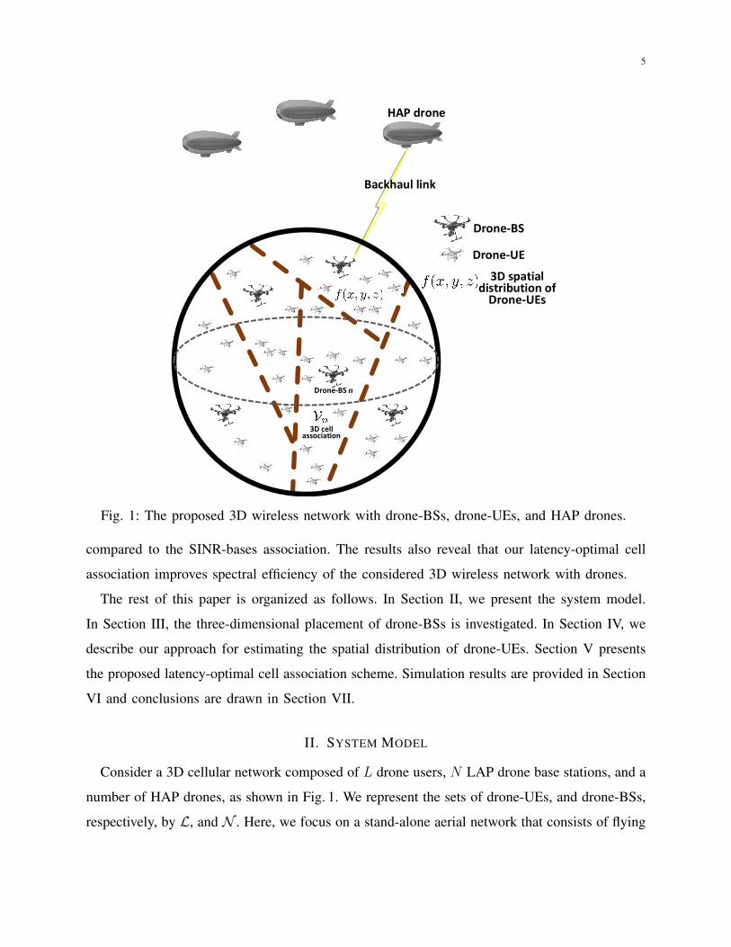
We consider the average latency in servicing drone-UEs as our main performance metric.
In particular, we consider transmission latency in drone-BSs to drone-UEs communications,
backhaul latency in drone-BSs to HAP drones links, and computation latency for drone-BSs that
serve drone-UEs. The transmission latency for a drone-UE located at (x, y, z) which is served
by drone-BS n is 3:
τTrn (x, y, z,Kn) =
β
Rn(x, y, z), (3)
where β is the number of bits per packet that must be transmitted to each drone-UE.
The backhaul latency depends on the load of drone-BSs and the backhaul transmission rates.
In this case, the average backhaul latency in drone-BS n to its corresponding HAP-drone
communications is given by:
τBn (Kn) =
βL
∫Vnf(x, y, z)dxdydz
Cn=βKn
Cn, (4)
where Cn is the maximum backhaul transmission rate for drone-BS n, and βL∫Vn f(x, y, z)dxdydz
represents the average load on drone-BS n.
The computation time depends on the data size (i.e., load) that must be processed in each
drone-BS, and the processing speed. To model the computational latency at drone-BS n, we use
function gn(βKn) with βKn being the total data size that must be processed at the drone-BS.
Therefore, the total latency experienced by any arbitrary drone-UE located at (x, y, z) while
being served by drone-BS n can be given by:
τ totn (x, y, z,Kn) = τTr
n (x, y, z,Kn) + τBn (Kn) + gn(βKn), (5)
Given this model, our goal is to minimize the average latency of drone-UEs by finding the
optimal 3D cell association in drone-BSs to drone-UEs communications. In particular, given the
3(3) represents the transmission latency which is the time required to transmit an entire packet [29].
8
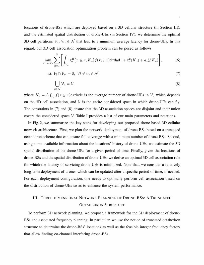
locations of drone-BSs which are deployed based on a 3D cellular structure (in Section III),
and the estimated spatial distribution of drone-UEs (in Section IV), we determine the optimal
3D cell partitions Vn, ∀n ∈ N that lead to a minimum average latency for drone-UEs. In this
regard, our 3D cell association optimization problem can be posed as follows:
minV1,...,VN
N∑n=1
[∫VnτTrn
(x, y, z,Kn
)f(x, y, z)dxdydz + τB
n (Kn) + gn(βKn)
], (6)
s.t. Vl ∩ Vm = ∅, ∀l 6= m ∈ N , (7)⋃n∈N
Vn = V , (8)
where Kn = L∫Vn f(x, y, z)dxdydz is the average number of drone-UEs in Vn which depends
on the 3D cell association, and V is the entire considered space in which drone-UEs can fly.
The constraints in (7) and (8) ensure that the 3D association spaces are disjoint and their union
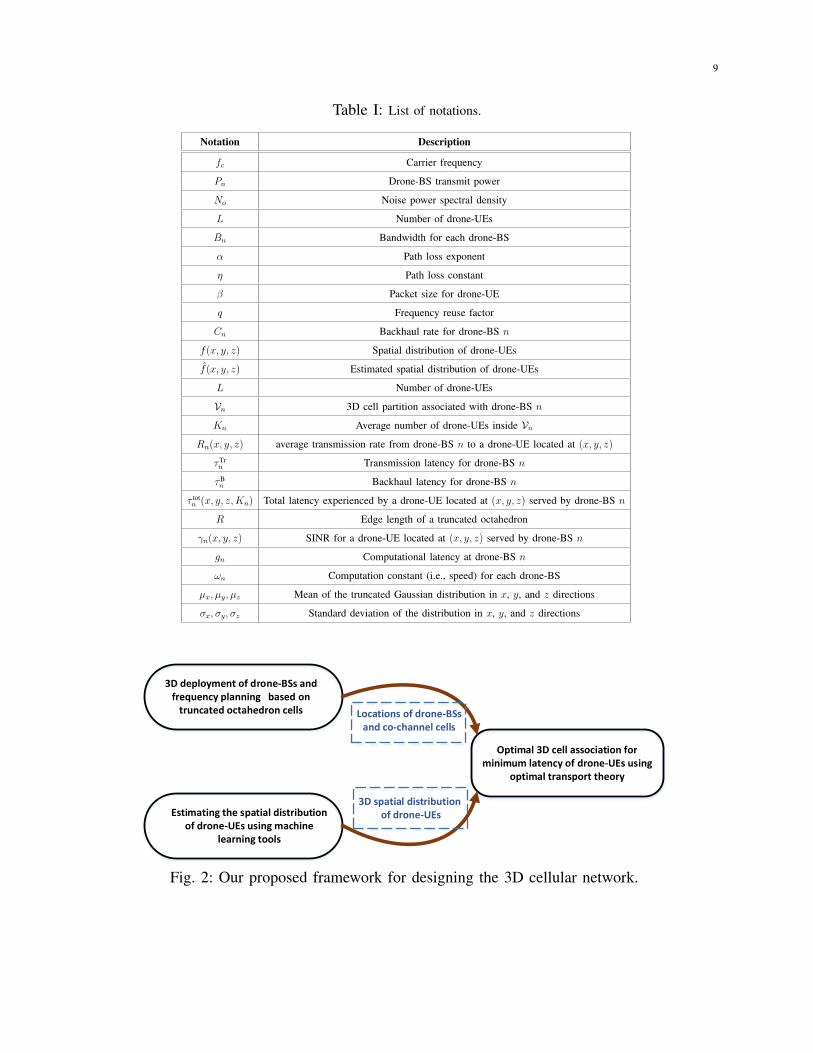
covers the considered space V . Table I provides a list of our main parameters and notations.
In Fig. 2, we summarize the key steps for developing our proposed drone-based 3D cellular
network architecture. First, we plan the network deployment of drone-BSs based on a truncated
octahedron scheme that can ensure full coverage with a minimum number of drone-BSs. Second,
using some available information about the locations’ history of drone-UEs, we estimate the 3D
spatial distribution of the drone-UEs for a given period of time. Finally, given the locations of
drone-BSs and the spatial distribution of drone-UEs, we derive an optimal 3D cell association rule
for which the latency of servicing drone-UEs is minimized. Note that, we consider a relatively
long-term deployment of drones which can be updated after a specific period of time, if needed.
For each deployment configuration, one needs to optimally perform cell association based on
the distribution of drone-UEs so as to enhance the system performance.
III. THREE-DIMENSIONAL NETWORK PLANNING OF DRONE-BSS: A TRUNCATED
OCTAHEDRON STRUCTURE
To perform 3D network planning, we propose a framework for the 3D deployment of drone-
BSs and associated frequency planning. In particular, we use the notion of truncated octahedron
structure to determine the drone-BSs’ locations as well as the feasible integer frequency factors
that allow finding co-channel interfering drone-BSs.
9
Table I: List of notations.
Notation Description
fc Carrier frequency
Pn Drone-BS transmit power
No Noise power spectral density
L Number of drone-UEs
Bn Bandwidth for each drone-BS
α Path loss exponent
η Path loss constant
β Packet size for drone-UE
q Frequency reuse factor
Cn Backhaul rate for drone-BS n
f(x, y, z) Spatial distribution of drone-UEs
f(x, y, z) Estimated spatial distribution of drone-UEs
L Number of drone-UEs
Vn 3D cell partition associated with drone-BS n
Kn Average number of drone-UEs inside VnRn(x, y, z) average transmission rate from drone-BS n to a drone-UE located at (x, y, z)
τTrn Transmission latency for drone-BS n
τBn Backhaul latency for drone-BS n
τ totn (x, y, z,Kn) Total latency experienced by a drone-UE located at (x, y, z) served by drone-BS n
R Edge length of a truncated octahedron
γn(x, y, z) SINR for a drone-UE located at (x, y, z) served by drone-BS n
gn Computational latency at drone-BS n
ωn Computation constant (i.e., speed) for each drone-BS
µx, µy, µz Mean of the truncated Gaussian distribution in x, y, and z directions
σx, σy, σz Standard deviation of the distribution in x, y, and z directions
3D deployment of drone-BSs and frequency planning based on
truncated octahedron cells
Estimating the spatial distribution of drone-UEs using machine
learning tools
Optimal 3D cell association for minimum latency of drone-UEs using
optimal transport theory
Locations of drone-BSs and co-channel cells
3D spatial distribution of drone-UEs
Fig. 2: Our proposed framework for designing the 3D cellular network.
10
RR
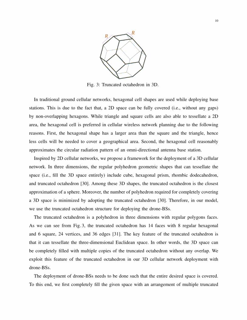
Fig. 3: Truncated octahedron in 3D.
In traditional ground cellular networks, hexagonal cell shapes are used while deploying base
stations. This is due to the fact that, a 2D space can be fully covered (i.e., without any gaps)
by non-overlapping hexagons. While triangle and square cells are also able to tessellate a 2D
area, the hexagonal cell is preferred in cellular wireless network planning due to the following
reasons. First, the hexagonal shape has a larger area than the square and the triangle, hence
less cells will be needed to cover a geographical area. Second, the hexagonal cell reasonably
approximates the circular radiation pattern of an omni-directional antenna base station.
Inspired by 2D cellular networks, we propose a framework for the deployment of a 3D cellular
network. In three dimensions, the regular polyhedron geometric shapes that can tessellate the
space (i.e., fill the 3D space entirely) include cube, hexagonal prism, rhombic dodecahedron,
and truncated octahedron [30]. Among these 3D shapes, the truncated octahedron is the closest
approximation of a sphere. Moreover, the number of polyhedron required for completely covering
a 3D space is minimized by adopting the truncated octahedron [30]. Therefore, in our model,
we use the truncated octahedron structure for deploying the drone-BSs.
The truncated octahedron is a polyhedron in three dimensions with regular polygons faces.
As we can see from Fig. 3, the truncated octahedron has 14 faces with 8 regular hexagonal
and 6 square, 24 vertices, and 36 edges [31]. The key feature of the truncated octahedron is
that it can tessellate the three-dimensional Euclidean space. In other words, the 3D space can
be completely filled with multiple copies of the truncated octahedron without any overlap. We
exploit this feature of the truncated octahedron in our 3D cellular network deployment with
drone-BSs.
The deployment of drone-BSs needs to be done such that the entire desired space is covered.
To this end, we first completely fill the given space with an arrangement of multiple truncated

11
Fig. 4: Deployment of drone-BSs based on truncated octahedron cells.
octahedron cells. Then, we place each drone-BS at the center of each truncated octahedron,
as shown in Fig. 4 as an illustrative example. Our proposed deployment approach can ensure
full coverage for a given 3D space and is also easy to implement and tractable. Moreover, our
approach facilitates frequency planning in 3D cellular networks by deriving analytical expressions
for the feasible integer reuse factors. Next, we determine the locations of drone-BSs based on
the proposed truncated octahedron cell structure.
Theorem 1. The three-dimensional locations of drone-BSs in the proposed 3D cellular network
are given by:
P a,b,c =[xo, yo, zo
]+√2R[a+ b− c,−a+ b+ c, a− b+ c
], (9)
where a, b, c are integers chosen from set ...,−2,−1, 0, 1, 2, ..., and R is the edge length of
the considered truncated octahedrons. [xo, yo, zo] is the Cartesian coordinates of a given reference
location (e.g., center of a specified space).
Proof. For the deployment of drone-BSs, we first create a 3D lattice of truncated octahedrons
and then, place each drone-BS at the center of each truncated octahedron. Hence, to determine
the locations of drone-BSs, we need to find the center of truncated octahedrons.
Let [xo, yo, zo] be the center of the first truncated octahedron in Cartesian coordinates with
the x, y, and z directions being perpendicular to square faces A3, A2, and A1 as shown in Fig.
5. We find a new coordinate system whose integer coordinates are the center of the truncated
octahedrons. By moving, in integer value steps, along the axes of this coordinate system, we
can reach the center of the truncated octahedrons. We consider a coordinate system whose axes

12
x y
z
A1
A3
A2
A4A5
A6
Fig. 5: Coordinate systems in drone-BSs deployment.
(e1, e2, e3) are vertically outward the hexagonal faces, A4, A5, and A6. Now, we find the
Euclidean length of each unit axis of this coordinate system. The distance between the center of
the truncated octahedron (e.g., [xo, yo, zo]) and each hexagonal face is R√6/2 [31]. Therefore,
the distance from [xo, yo, zo] to the center of an adjacent truncated octahedron connecting to
face A4 is R√6. As a result, each unit on axis e1 (and also e2 and e3) must be 2R
√6. It can
be easily verified that the centers of the truncated octahedrons in the 3D lattice are the integer
coordinates of the (e1,e2,e3) coordinate system. Hence, the 3D location of each drone-BS can
be represented by a triple (a, b, c) with a, b, and c being integers. The position of a drone-BS
obtained by a, b, c is given by:
P a,b,c = ae1 + be2 + ce3. (10)
Now, we need to represent P a,b,c using Cartesian coordinates. To this end, we find the projection
of e1, e2, and e3 on the x, y, and z axes. With some geometric calculations and using the fact
that the dihedral angle (i.e., angle between two intersecting planes) between the adjacent square
face and hexagonal face is cos−1(−1√3) [31], we obtain:
e1 = R√6(−1√
3x+ 1√
3y + 1√
3z),
e2 = R√6(
1√3x+ −1√
3y + 1√
3z),
e3 = R√6(
1√3x+ 1√
3y + −1√
3z).
(11)
Finally, using (10) and (11), the 3D locations of drone-BSs in Cartesian coordinates, with respect
to the reference position [xo, yo, zo] are given by:
P a,b,c =[xo, yo, zo
]+√2R[a+ b− c,−a+ b+ c, a− b+ c
], (12)
13
which proves the theorem.
Using Theorem 1, we can find the 3D coordinates of drone-BSs which are deployed at the
centers of truncated octahedrons. Moreover, as shown next, Theorem 1 allows us to determine
the frequency reuse factor as well as interfering drone-BSs in the proposed 3D cellular network.
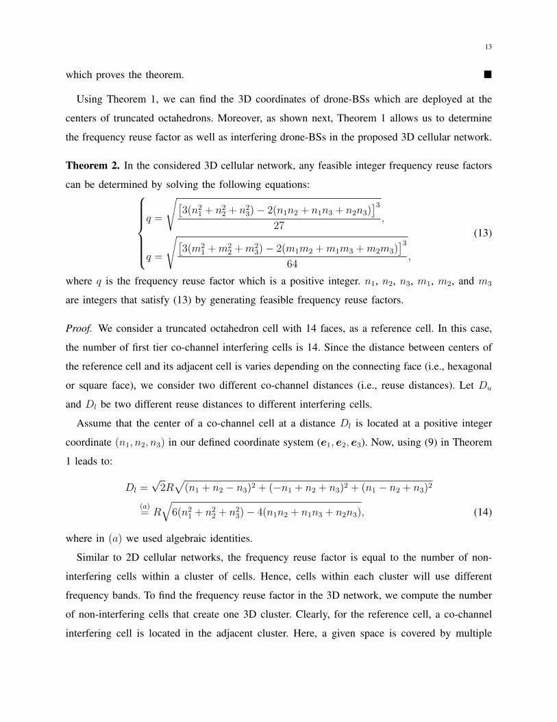
Theorem 2. In the considered 3D cellular network, any feasible integer frequency reuse factors
can be determined by solving the following equations:q =
√[3(n2
1 + n22 + n2
3)− 2(n1n2 + n1n3 + n2n3)]3
27,
q =
√[3(m2
1 +m22 +m2
3)− 2(m1m2 +m1m3 +m2m3)]3
64,
(13)
where q is the frequency reuse factor which is a positive integer. n1, n2, n3, m1, m2, and m3
are integers that satisfy (13) by generating feasible frequency reuse factors.
Proof. We consider a truncated octahedron cell with 14 faces, as a reference cell. In this case,
the number of first tier co-channel interfering cells is 14. Since the distance between centers of
the reference cell and its adjacent cell is varies depending on the connecting face (i.e., hexagonal
or square face), we consider two different co-channel distances (i.e., reuse distances). Let Du
and Dl be two different reuse distances to different interfering cells.
Assume that the center of a co-channel cell at a distance Dl is located at a positive integer
coordinate (n1, n2, n3) in our defined coordinate system (e1, e2, e3). Now, using (9) in Theorem
1 leads to:
Dl =√2R√
(n1 + n2 − n3)2 + (−n1 + n2 + n3)2 + (n1 − n2 + n3)2
(a)= R
√6(n2
1 + n22 + n2
3)− 4(n1n2 + n1n3 + n2n3), (14)
where in (a) we used algebraic identities.
Similar to 2D cellular networks, the frequency reuse factor is equal to the number of non-
interfering cells within a cluster of cells. Hence, cells within each cluster will use different
frequency bands. To find the frequency reuse factor in the 3D network, we compute the number
of non-interfering cells that create one 3D cluster. Clearly, for the reference cell, a co-channel
interfering cell is located in the adjacent cluster. Here, a given space is covered by multiple
14
Big truncated octahedron cell
Small truncated octahedron cell
Cluster
Cluster
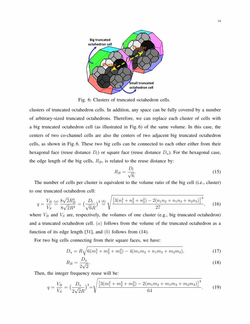
Fig. 6: Clusters of truncated octahedron cells.
clusters of truncated octahedron cells. In addition, any space can be fully covered by a number
of arbitrary-sized truncated octahedrons. Therefore, we can replace each cluster of cells with
a big truncated octahedron cell (as illustrated in Fig. 6) of the same volume. In this case, the
centers of two co-channel cells are also the centers of two adjacent big truncated octahedron
cells, as shown in Fig. 6. These two big cells can be connected to each other either from their
hexagonal face (reuse distance Dl) or square face (reuse distance Du). For the hexagonal case,
the edge length of the big cells, RB, is related to the reuse distance by:
RB =Dl√6. (15)
The number of cells per cluster is equivalent to the volume ratio of the big cell (i.e., cluster)
to one truncated octahedron cell:
q =VBVS
(a)=
8√2R3
B
8√2R3
=( Dl√
6R
)3 (b)=
√[3(n2
1 + n22 + n2
3)− 2(n1n2 + n1n3 + n2n3)]3
27, (16)
where VB and VS are, respectively, the volumes of one cluster (e.g., big truncated octahedron)
and a truncated octahedron cell. (a) follows from the volume of the truncated octahedron as a
function of its edge length [31], and (b) follows from (14).
For two big cells connecting from their square faces, we have:
Du = R√
6(m21 +m2
2 +m23)− 4(m1m2 + n1m3 +m2m3), (17)
RB =Du
2√2. (18)
Then, the integer frequency reuse will be:
q =VBVS
=( Du
2√2R
)3=
√[3(m2
1 +m22 +m2
3)− 2(m1m2 +m1m3 +m2m3)]3
64. (19)
15
Since the number of cells per cluster represents the frequency reuse factor is a positive integer,
(n1, n2, n3) and (m1,m2,m3) must generate an integer in (16) and (19).
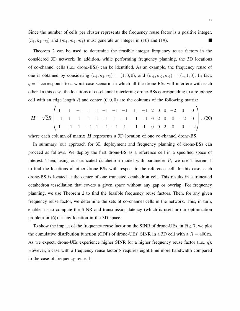
Theorem 2 can be used to determine the feasible integer frequency reuse factors in the
considered 3D network. In addition, while performing frequency planning, the 3D locations
of co-channel cells (i.e., drone-BSs) can be identified. As an example, the frequency reuse of
one is obtained by considering (n1, n2, n3) = (1, 0, 0), and (m1,m2,m3) = (1, 1, 0). In fact,
q = 1 corresponds to a worst-case scenario in which all the drone-BSs will interfere with each
other. In this case, the locations of co-channel interfering drone-BSs corresponding to a reference
cell with an edge length R and center (0, 0, 0) are the columns of the following matrix:
H =√2R
1 1 −1 1 1 −1 −1 −1 1 −1 2 0 0 −2 0 0
−1 1 1 1 1 −1 1 −1 −1 −1 0 2 0 0 −2 0
1 −1 1 −1 1 −1 −1 1 −1 1 0 0 2 0 0 −2
, (20)
where each column of matrix H represents a 3D location of one co-channel drone-BS.
In summary, our approach for 3D deployment and frequency planning of drone-BSs can
proceed as follows. We deploy the first drone-BS as a reference cell in a specified space of
interest. Then, using our truncated octahedron model with parameter R, we use Theorem 1
to find the locations of other drone-BSs with respect to the reference cell. In this case, each
drone-BS is located at the center of one truncated octahedron cell. This results in a truncated
octahedron tessellation that covers a given space without any gap or overlap. For frequency
planning, we use Theorem 2 to find the feasible frequency reuse factors. Then, for any given
frequency reuse factor, we determine the sets of co-channel cells in the network. This, in turn,
enables us to compute the SINR and transmission latency (which is used in our optimization
problem in (6)) at any location in the 3D space.
To show the impact of the frequency reuse factor on the SINR of drone-UEs, in Fig. 7, we plot
the cumulative distribution function (CDF) of drone-UEs’ SINR in a 3D cell with a R = 400m.
As we expect, drone-UEs experience higher SINR for a higher frequency reuse factor (i.e., q).
However, a case with a frequency reuse factor 8 requires eight time more bandwidth compared
to the case of frequency reuse 1.

16
−5 0 5 10 15 200
0.2
0.4
0.6
0.8
1
SINR (dB)
CD
F o
f SIN
R
q=1
q=8
Fig. 7: CDF of drone-UEs’ SINR in a 3D cell for two different frequency reuse factors.
IV. ESTIMATION OF THE SPATIAL DISTRIBUTION OF DRONE-UES
Since drone-UEs cannot continuously report their locations due to excessive overhead costs,
we need to design a machine learning based mechanism for estimating the locations of drone-
UEs using sparse information. Therefore, we assume that each drone-UE is able to report its
location at each T seconds. Then, using that, we estimate the spatial distribution of drone-UEs
which remains valid for the next T seconds. We should note that, during T seconds, the location
of each drone-UE is changing due to its mobility. However, the distribution of drone-UEs is
fixed so that we can use our estimation for the period of T seconds. To this end, we develop
a nonparametric model for f(x, y, z) using a kernel density estimation (KDE) [32]. In case of
parametric density estimation methods, if one uses a poor assumption for the density model, it
results in a poor estimation performance. However, nonparametric methods are not sensitive to
such poor assumptions.
The distribution of drone-UEs changes with time. Nevertheless, since we assume that this
distribution is fixed within an interval of T seconds, we sample the location of each drone-UE
every T seconds, and use it to estimate f(x, y, z). This reduces overhead compared to the case
in which the system knows the location of drone-UEs at every time instant. We consider some
small regions R where each drone lies in with probability p. Hence, the number of drone-UEs
in this region K follows a binomial distribution, i.e.,
Pr(K) =L!
(L−K)!K!pK(1− p)L−K , (21)

17
For a binomial distribution, we know that the mean is E(KL) = p. Thus, we can write:
limL→∞
K
L= p. (22)
Therefore, for a large L, we can assume K = Lp. Since R is a small region, we can assume
that f(x, y, z),∀(x, y, z) ∈ R is constant, and hence:
p =
∫Rf(x, y, z)dxdydz = f(x, y, z)VR, (23)
where VR is the volume of region R. Combining (22) and (23), we can write:
f(x, y, z) =K
LVR. (24)
If we define a small region R as a cube:
C( xhx,y
hy,z
hz) =
1, max| xhx|, | y
hy|, | z
hz| ≤ 1/2,
0, otherwise,(25)
then, we can write the total number of users inside this cube as:
K =L∑i=1
C(x− xih
,y − yih
,z − zih
)= Lhxhyhzf(x, y, z). (26)
Since the volume of the cube in (25) is hx · hy · hz, we can write the density function as:
f(x, y, z) =1
L
L∑i=1
1
hxhyhzC(x− xihx
,y − yihy
,z − zihz
), (27)
which can be interpreted as L cubes with the volume hx · hy · hz centered at each data point.
Also, hx, hy, and hz are the widths of the kernel in dimensions x, y, and z, respectively. To
remove the discontinuity of cubes in the space, we use Gaussian kernels [33]. If we approximate
each cube in (27) with a Gaussian kernel, we have:
f(x, y, z) =1
L
L∑i=1
1√(2π)3hxhyhz
e−(
(x−xi)2
hx+
(y−yi)2
hy+
(z−zi)2
hz
). (28)
f(x, y, z) is not equal to f(x, y, z), for two reasons. First, L is a finite number, and second,
the Gaussian kernel is an approximation of the cube in (25). However, we will see that this
estimation has small errors even when the value of L is not large. We assume that x, y, and
z are uncorrelated, and hence, all the off-diagonal elements of the covariance matrix are zero.
Here, the parameters hx, hy, and hz have a major effect on the accuracy of the estimation and
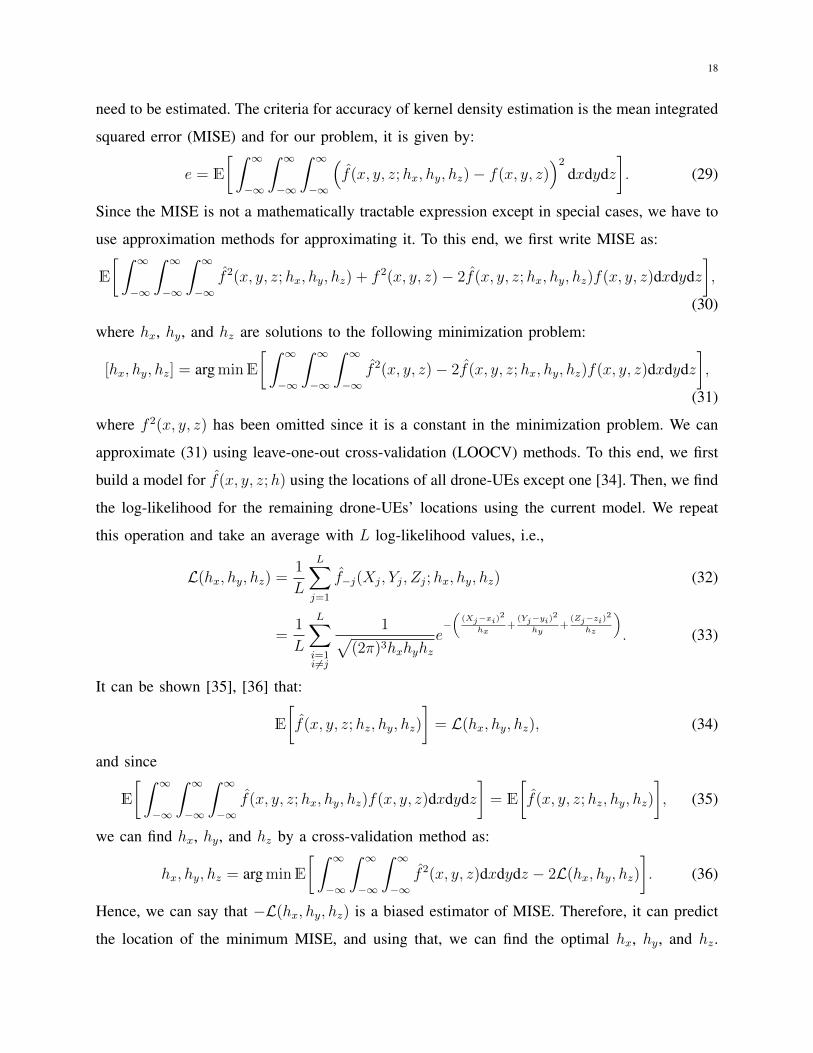
18
need to be estimated. The criteria for accuracy of kernel density estimation is the mean integrated
squared error (MISE) and for our problem, it is given by:
e = E
[ ∫ ∞−∞
∫ ∞−∞
∫ ∞−∞
(f(x, y, z;hx, hy, hz)− f(x, y, z)
)2dxdydz
]. (29)
Since the MISE is not a mathematically tractable expression except in special cases, we have to
use approximation methods for approximating it. To this end, we first write MISE as:
E
[ ∫ ∞−∞
∫ ∞−∞
∫ ∞−∞
f 2(x, y, z;hx, hy, hz) + f 2(x, y, z)− 2f(x, y, z;hx, hy, hz)f(x, y, z)dxdydz],
(30)
where hx, hy, and hz are solutions to the following minimization problem:
[hx, hy, hz] = argminE
[ ∫ ∞−∞
∫ ∞−∞
∫ ∞−∞
f 2(x, y, z)− 2f(x, y, z;hx, hy, hz)f(x, y, z)dxdydz],
(31)
where f 2(x, y, z) has been omitted since it is a constant in the minimization problem. We can
approximate (31) using leave-one-out cross-validation (LOOCV) methods. To this end, we first
build a model for f(x, y, z;h) using the locations of all drone-UEs except one [34]. Then, we find
the log-likelihood for the remaining drone-UEs’ locations using the current model. We repeat
this operation and take an average with L log-likelihood values, i.e.,
L(hx, hy, hz) =1
L
L∑j=1
f−j(Xj, Yj, Zj;hx, hy, hz) (32)
=1
L
L∑i=1i 6=j
1√(2π)3hxhyhz
e−(
(Xj−xi)2
hx+
(Yj−yi)2
hy+
(Zj−zi)2
hz
). (33)
It can be shown [35], [36] that:
E
[f(x, y, z;hz, hy, hz)
]= L(hx, hy, hz), (34)
and since
E
[ ∫ ∞−∞
∫ ∞−∞
∫ ∞−∞
f(x, y, z;hx, hy, hz)f(x, y, z)dxdydz]= E
[f(x, y, z;hz, hy, hz)
], (35)
we can find hx, hy, and hz by a cross-validation method as:
hx, hy, hz = argminE
[ ∫ ∞−∞
∫ ∞−∞
∫ ∞−∞
f 2(x, y, z)dxdydz − 2L(hx, hy, hz)]. (36)
Hence, we can say that −L(hx, hy, hz) is a biased estimator of MISE. Therefore, it can predict
the location of the minimum MISE, and using that, we can find the optimal hx, hy, and hz.

19
Algorithm 1 drone-UEs’ distribution estimation algorithmInput: drone-UEs location (X1, Y1, Z1) · · · , (XL, YL, ZL)
Output: f(x, y, z)
Initialize: H ← set of candidate for hx, hy, hz, L(hbest)←∞
for hx, hy, hz ∈ H do
for j = 1, · · · , L do
Build a model using (28) with Xi, i ∈ 1, · · · , L, i 6= j
sum← sum+ 12log hx +
12log hy +
12log hz +
((Xj−xi)2
hx+
(Yj−yi)2
hy+
(Zj−zi)2
hz
)+ 3
2log(2π)
end for
L(hx, hy, hz)← 1L
sum
if L(hx, hy, hz) ≤ L(hbest) then
hbest ← hx, hy, hz
end if
end for
hx, hy, hz ← hbest
return f(x, y, z;hx, hy, hz) in (28) as drone-UEs PDF
0.2 0.4 0.6 0.8 1 1.2 1.40.5
1
1.5
2
2.5x 10
−3
Kernel width
Mea
n in
tegr
ated
squ
ared
err
or (
MIS
E)
Fig. 8: MISE for symmetric kernel widths (hx = hy = hz = h).
Algorithm 1 summarizes the estimation of f(x, y, z) using location of drone-UEs in each T
seconds.
Fig. 8 shows the MISE in case of symmetric kernels (hx = hy = hz = h) for 30 drone-UEs for
different values of h. As we can see, our algorithm can potentially minimize the MISE to a value
of 7.9554× 10−04. Fig. 9 shows the negative log-likelihood function. As we can see from Figs.
8 and 9, −L(hx, hy, hz) is a biased estimator of MISE, and hence, we can use −L(hx, hy, hz) to
find the optimal hx, hy, hz. Fig. 9 shows that, by means of LOOCV method, the MISE for our

20
0 1 2 3 4 5
6
8
10
12
14
Kernel width
Neg
ativ
e lo
g lik
elih
ood
Fig. 9: LOOCV method for finding an optimal kernel width (h).
PDF estimation is 5.7221×10−04 which is close to the MISE lower bound that is 7.9554×10−04.
In summary, our approach for estimation of drone-UE spatial distribution is as follows. We
collect the location of drone-UEs at each T seconds. Then, we estimate the distribution of drone-
UEs to use it for 3D cell association during the next T seconds. We adopt an accuracy metric
for our density estimation and use it to find width of the kernels. We showed that our approach
is able to estimate the spatial distribution of drone-UEs with a near optimal accuracy.
V. OPTIMAL 3D CELL ASSOCIATION FOR MINIMUM LATENCY
In Sections III and IV, we determined the locations of drone-BSs and the spatial distribution of
drone-UEs. Here, we use this information (i.e., drone-BSs’ locations and drone-UEs’ distribution)
to explicitly formulate our latency-optimal 3D cell association problem.
minV1,...,VN
N∑n=1
[∫Vn
βKn
Bn log2(1 + γn(x, y, z)
) f(x, y, z)dxdydz +βKn
Cn+ gn(βKn)
], (37)
s.t. Kn = L
∫Vnf(x, y, z)dxdydz, (38)
Vl ∩ Vm = ∅, ∀l 6= m ∈ N , (39)⋃n∈N
Vn = V , (40)
where γn(x, y, z) is the downlink SINR for a drone-UE located at (x, y, z) which is served by
drone-BS n. Considering a practical bounded path loss model [37] for air-to-air communications,

21
the SINR can be given by:
γn(x, y, z) =ηκn(x, y, z)Pn[1 + dn(x, y, z)]
−α∑u∈Iint
ηκu(x, y, z)Pu[1 + du(x, y, z)]−α +NoBn
, (41)
dn(x, y, z) =√(x− xn)2 + (y − yn)2 + (z − zn)2, (42)
du(x, y, z) =√
(x− xu)2 + (y − yu)2 + (z − zu)2, u ∈ Iint, (43)
where κn(x, y, z) is a channel gain factor between a drone-UE, located at (x, y, z), and drone-BS
n. κn(x, y, z) depends on the environment, and the locations of the drone-UE and drone-BS.
κn(x, y, z) = 1 corresponds to a LoS air-to-air communication, while 0 < κn(x, y, z) < 1 can
capture the impact of NLoS conditions. α is the path loss exponent, No is the noise power
spectral density, η is the path loss constant, and (xn, yn, zn) is the 3D location of drone-BS n.
dn(x, y, z) and du(x, y, z) are, respectively, the distance of drone-BSs n and u with a drone-UE
located at (x, y, z). Also, Iint is the set of co-channel interfering drone-BSs that operate over the
same frequency band as drone-BS n.
Solving (37) is challenging since the optimization variables Vn, ∀n ∈ N , are continuous 3D
association spaces which are mutually dependent. Furthermore, the fact that the size and shape of
these 3D association spaces are unknown, exacerbates the complexity. In addition, the objective
function in (37) does not have a closed-form expression thus making the problem intractable.
Consequently, employing traditional optimization techniques (e.g., convex optimization) are not
sufficient to solve (37). Here, we tackle our 3D space association by exploiting optimal transport
theory. In particular, first, we prove the existence of an optimal solution to (37) and, then, we
completely characterize the solution space. We note that, compared to our previous work in
[19], this work is different in terms of the system model, the 3D cell association optimization
problem, as well as the solution.
Optimal transport theory is a mathematical tool that is used to find an optimal mapping between
two arbitrary probability measures [38]. More specifically, in a semi-discrete optimal transport
problem, a continuous probability density function must be mapped to a discrete probability
measure. In such a semi-discrete case, the optimal transport map will optimally partition the
continuous distribution and assign each partition to one point in the discrete probability measure
(which, in our case, is the discrete set of drone-BSs).

22
Our cell association problem can be modeled as a semi-discrete optimal transport problem in
which the source measure (drone-UEs’ distribution) is continuous while the destination (distri-
bution of drone-BSs) is discrete. Then, the optimal 3D cell partitions are obtained by optimally
mapping the drone-UEs to drone-BSs.
Lemma 1. The optimization problem in (37) admits an optimal solution for any semi-continuous
function gn(.), n ∈ N .
Proof. Consider Kn = L∫Vn f(x, y, z)dxdydz and the following simplex:
S=
K = (K1, K2, ..., KN)∈ RN ;
N∑n=1
Kn = L,Kn ≥ 0,∀n ∈ N
. (44)
Given any vector K, the optimization problem in (37) can be represented by:
minV1,...,VN
N∑n=1
∫Vnc(v, sn)f(v)dv, (45)
s.t.∫Vnf(v)dv =
Kn
L, (46)
Vl ∩ Vm = ∅, ∀l 6= m ∈ N ,⋃n∈N
Vn = V , (47)
where sn is the location of drone-BS n, v = (x, y, z), and c(v, sn) = βKn
Bn log2
(1+γn(x,y,z)
) +
LKn
(βKnCn
+ gn(βKn)).
This optimization problem is equivalent to the following semi-discrete optimal transport
problem:
minT
∫Vc (v, s)f(v)dv, s = T (v), (48)
where s is the location of a drone-BS, and T (.) is the transport map which is related to 3D cell
partition Vn by: T (v) =
N∑n=1
sn1Vn(v);
∫Vnf(v)dv =
Kn
L
. (49)
Considering the fact that for any semi-discrete optimal transport problem with a lower semi-
continuous cost function an optimal transport map exists [38], [39], (45) admits an optimal
solution for any K ∈ S. Also, since S is a simplex (which is a non-empty and compact set),
problem (37) admits an optimal solution over the entire S. This proves Lemma 1.
Next, given the existence of the optimal solution, we characterize the solution.
23
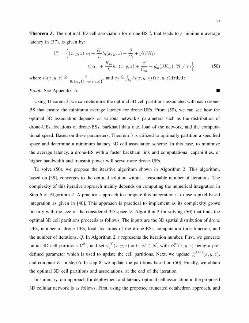
Theorem 3. The optimal 3D cell association for drone-BS l, that leads to a minimum average
latency in (37), is given by:
V∗l =(x, y, z)
∣∣αl + Kl
Lhl(x, y, z) +
β
Cl+ g′l(βKl)
≤ αm +Km
Lhm(x, y, z) +
β
Cm+ g′m(βKm), ∀l 6= m
, (50)
where hl(x, y, z) , β
Bl log2
(1+γl(x,y,z)
) , and αl ,∫Vlhl(x, y, x)f(x, y, z)dxdydz.
Proof. See Appendix A.
Using Theorem 3, we can determine the optimal 3D cell partitions associated with each drone-
BS that ensure the minimum average latency for drone-UEs. From (50), we can see how the
optimal 3D association depends on various network’s parameters such as the distribution of
drone-UEs, locations of drone-BSs, backhaul data rate, load of the network, and the computa-
tional speed. Based on these parameters, Theorem 3 is utilized to optimally partition a specified
space and determine a minimum latency 3D cell association scheme. In this case, to minimize
the average latency, a drone-BS with a faster backhaul link and computational capabilities, or
higher bandwidth and transmit power will serve more drone-UEs.
To solve (50), we propose the iterative algorithm shown in Algorithm 2. This algorithm,
based on [39], converges to the optimal solution within a reasonable number of iterations. The
complexity of this iterative approach mainly depends on computing the numerical integration in
Step 6 of Algorithm 2. A practical approach to compute this integration is to use a pixel-based
integration as given in [40]. This approach is practical to implement as its complexity grows
linearly with the size of the considered 3D space V . Algorithm 2 for solving (50) that finds the
optimal 3D cell partitions proceeds as follows. The inputs are the 3D spatial distribution of drone
UEs, number of drone-UEs, load, locations of the drone-BSs, computation time function, and
the number of iterations, Q. In Algorithm 2, t represents the iteration number. First, we generate
initial 3D cell partitions V(t)l , and set ψ(t)
l (x, y, z) = 0, ∀l ∈ N , with ψ(t)l (x, y, z) being a pre-
defined parameter which is used to update the cell partitions. Next, we update ψ(t+1)l (x, y, z),
and compute Kl in step 6. In step 8, we update the partitions based on (50). Finally, we obtain
the optimal 3D cell partitions and associations, at the end of the iteration.
In summary, our approach for deployment and latency-optimal cell association in the proposed
3D cellular network is as follows. First, using the proposed truncated octahedron approach, and
24
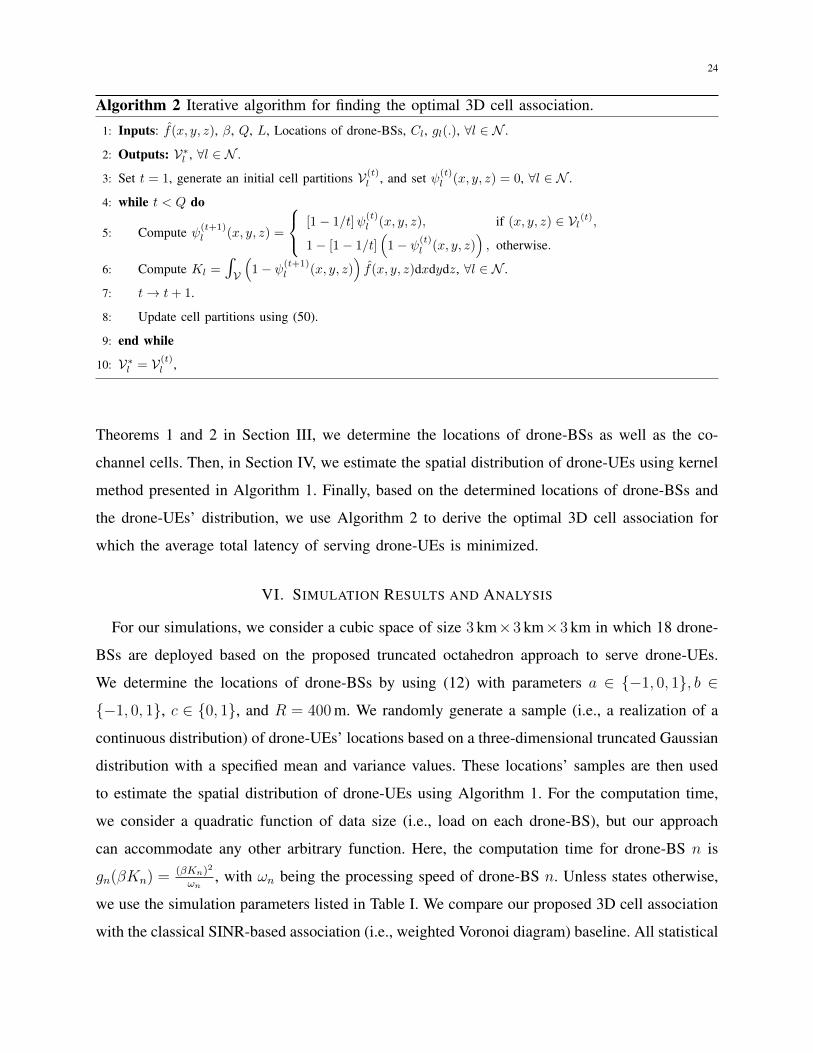
Algorithm 2 Iterative algorithm for finding the optimal 3D cell association.
1: Inputs: f(x, y, z), β, Q, L, Locations of drone-BSs, Cl, gl(.), ∀l ∈ N .
2: Outputs: V∗l , ∀l ∈ N .
3: Set t = 1, generate an initial cell partitions V(t)l , and set ψ(t)
l (x, y, z) = 0, ∀l ∈ N .
4: while t < Q do
5: Compute ψ(t+1)l (x, y, z) =
[1− 1/t]ψ(t)l (x, y, z), if (x, y, z) ∈ Vl(t),
1− [1− 1/t](1− ψ(t)
l (x, y, z)), otherwise.
6: Compute Kl =∫V
(1− ψ(t+1)
l (x, y, z))f(x, y, z)dxdydz, ∀l ∈ N .
7: t→ t+ 1.
8: Update cell partitions using (50).
9: end while
10: V∗l = V(t)
l ,
Theorems 1 and 2 in Section III, we determine the locations of drone-BSs as well as the co-
channel cells. Then, in Section IV, we estimate the spatial distribution of drone-UEs using kernel
method presented in Algorithm 1. Finally, based on the determined locations of drone-BSs and
the drone-UEs’ distribution, we use Algorithm 2 to derive the optimal 3D cell association for
which the average total latency of serving drone-UEs is minimized.
VI. SIMULATION RESULTS AND ANALYSIS
For our simulations, we consider a cubic space of size 3 km×3 km×3 km in which 18 drone-
BSs are deployed based on the proposed truncated octahedron approach to serve drone-UEs.
We determine the locations of drone-BSs by using (12) with parameters a ∈ −1, 0, 1, b ∈
−1, 0, 1, c ∈ 0, 1, and R = 400m. We randomly generate a sample (i.e., a realization of a
continuous distribution) of drone-UEs’ locations based on a three-dimensional truncated Gaussian
distribution with a specified mean and variance values. These locations’ samples are then used
to estimate the spatial distribution of drone-UEs using Algorithm 1. For the computation time,
we consider a quadratic function of data size (i.e., load on each drone-BS), but our approach
can accommodate any other arbitrary function. Here, the computation time for drone-BS n is
gn(βKn) =(βKn)2
ωn, with ωn being the processing speed of drone-BS n. Unless states otherwise,
we use the simulation parameters listed in Table I. We compare our proposed 3D cell association
with the classical SINR-based association (i.e., weighted Voronoi diagram) baseline. All statistical

25
Table II: Simulation parameters.
Parameter Description Value
fc Carrier frequency 2 GHz
Pn Drone-BS transmit power 0.5 W
No Noise power spectral density -170 dBm/Hz
L Number of drone-UEs 200
Bn Bandwidth for each drone-BS 10 MHz
α Path loss exponent 2
η Path loss constant 1.42× 10⁻⁴
β Packet size for drone-UE 10 kb
q Frequency reuse factor 1
Cn Backhaul rate for drone-BS n (100 + n) Mb/s
ωn Computation constant (i.e., speed) for each drone-BS 102 Tb/s
µx, µy, µz Mean of the truncated Gaussian distribution in x, y, and z directions 1000 m, 1000 m, 1000 m
σx, σy, σz Standard deviation of the distribution in x, y, and z directions 600 m, 600 m, 600 m
κn Channel gain factor 1
results are averaged over a large number of independent runs.
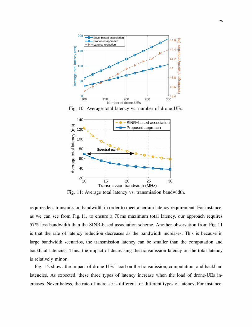
Fig. 10 shows the average total latency as a function of the number of drone-UEs for the
proposed 3D cell association and the SINR-based association schemes. As we can see from this
figure, the total latency increases by increasing the number of drone-UEs. A higher number of
drone-UEs leads to a higher network congestion which, in turn, increases transmission time,
backhaul latency, and computation time. Fig. 10 shows that, when the number of drone-UEs
increases from 200 to 300, the total latency increases by 56% and 42% for the SINR-based
association and the proposed approach. Moreover, we can see that our proposed approach
significantly reduces the latency compared to the SINR association case. This is due to the fact
that, in our approach, besides SINR, the impact of congestion on the transmission, backhaul,
and computational latencies is also taken into account. The proposed approach avoids creating
highly congested 3D cell partitions that can cause excessive latency. From Fig. 10, we can see
that our approach yields, on the average, 43.9% reduction in the average total latency compared
to the SINR-based association.
Fig. 11 shows how the latency can be reduced by increasing the transmission bandwidth. By
using more bandwidth, the transmission rate increases and, hence, the transmission latency de-
creases. Fig. 11 also reveals that our approach significantly enhances spectral efficiency compared
to the SINR-based association. In essence, compared to the SINR case, the proposed approach
26
100 150 200 250 300Number of drone-UEs
0
50
100
150
200
Ave
rage
tota
l lat
ency
(m
s)
43.4
43.6
43.8
44
44.2
44.4
44.6
Per
cent
age
of la
tenc
y re
duct
ion
(%
)SINR-based associationProposed approachLatency reduction
Fig. 10: Average total latency vs. number of drone-UEs.
10 15 20 25 3020
40
60
80
100
120
140
Transmission bandwidth (MHz)
Ave
rage
tota
l lat
ency
(m
s)
SINR−based associationProposed approach
Spectral gain
Fig. 11: Average total latency vs. transmission bandwidth.
requires less transmission bandwidth in order to meet a certain latency requirement. For instance,
as we can see from Fig. 11, to ensure a 70 ms maximum total latency, our approach requires
57% less bandwidth than the SINR-based association scheme. Another observation from Fig. 11
is that the rate of latency reduction decreases as the bandwidth increases. This is because in
large bandwidth scenarios, the transmission latency can be smaller than the computation and
backhaul latencies. Thus, the impact of decreasing the transmission latency on the total latency
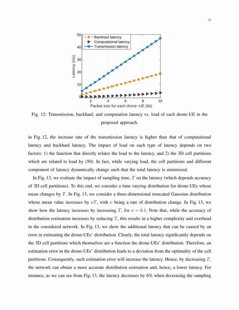
is relatively minor.Fig. 12 shows the impact of drone-UEs’ load on the transmission, computation, and backhaul
latencies. As expected, these three types of latency increase when the load of drone-UEs in-
creases. Nevertheless, the rate of increase is different for different types of latency. For instance,
27
2 4 6 8 100
10
20
30
40
50
Packet size for each drone−UE (kb)
Late
ncy
(ms)
Backhaul latencyComputational latencyTransmission latency
Fig. 12: Transmission, backhaul, and computation latency vs. load of each drone-UE in the
proposed approach.
in Fig. 12, the increase rate of the transmission latency is higher than that of computational
latency and backhaul latency. The impact of load on each type of latency depends on two
factors: 1) the function that directly relates the load to the latency, and 2) the 3D cell partitions
which are related to load by (50). In fact, while varying load, the cell partitions and different
component of latency dynamically change such that the total latency is minimized.
In Fig. 13, we evaluate the impact of sampling time, T on the latency (which depends accuracy
of 3D cell partitions). To this end, we consider a time varying distribution for drone-UEs whose
mean changes by T . In Fig. 13, we consider a three-dimensional truncated Gaussian distribution
whose mean value increases by νT , with ν being a rate of distribution change. In Fig. 13, we
show how the latency increases by increasing T , for ν = 0.1. Note that, while the accuracy of
distribution estimation increases by reducing T , this results in a higher complexity and overhead
in the considered network. In Fig. 13, we show the additional latency that can be caused by an
error in estimating the drone-UEs’ distribution. Clearly, the total latency significantly depends on
the 3D cell partitions which themselves are a function the drone-UEs’ distribution. Therefore, an
estimation error in the drone-UEs’ distribution leads to a deviation from the optimality of the cell
partitions. Consequently, such estimation error will increase the latency. Hence, by decreasing T ,
the network can obtain a more accurate distribution estimation and, hence, a lower latency. For
instance, as we can see from Fig. 13, the latency decreases by 6% when decreasing the sampling

28
0 5 10 15 20 25 30Sampling time (T) [min]
0
2
4
6
8
10
12
14
16
Add
ition
al la
tenc
y (%
)
= 5 m/min= 10 m/min
Fig. 13: Additional latency vs. sampling time for distribution estimation (T )
1 2 3 4 5 6 7 8 9 1020
40
60
80
100
120
Iteration number
Ave
rage
tota
l lat
ency
(m
in)
Fig. 14: Convergence of Algorithm 2.
time from 20 minutes to 10 minutes, for ν = 10m/min.
Finally, in Fig. 14, we show the convergence of Algorithm 2 that is used to find the optimal
3D cell association by iteratively solving (50). As we can see from this figure, Algorithm 2
converges within 6 iterations.
VII. CONCLUSION
In this paper, we have introduced a novel framework for cell association and deployment
in 3D cellular networks with drone-BSs and drone-UEs. We have proposed a tractable method
for the 3D deployment of drone-BSs and solved the problem of cell association with the goal
of minimizing the latency of drone users. For deployment, we have determined the drone-BSs’
locations based on a truncated octahedron structure and derived the feasible frequency reuse factor
29
in the considered 3D network. For latency-minimal cell association, first, we have estimated
the spatial distribution of the drone-UEs using the kernel density estimation method. Then,
using the estimated distribution of drone-UEs and the location of drone-BSs, we have derived
the optimal cell association of drone-UEs using optimal transport theory such that the latency
for drone-UEs is minimized. Our results have shown that the proposed approach significantly
reduces the latency of drone-UEs compared to the classical SINR-based association. Furthermore,
the proposed latency-optimal cell association improves the spectral efficiency of the 3D drone-
enabled wireless networks.
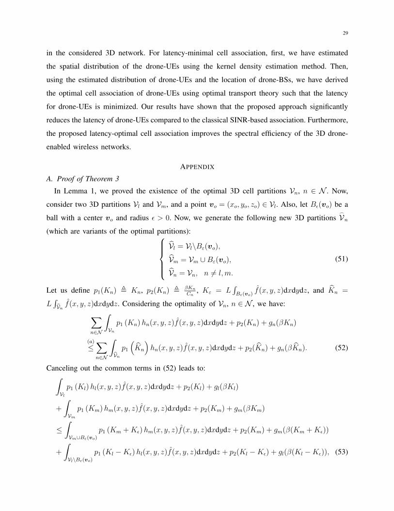
APPENDIX
A. Proof of Theorem 3
In Lemma 1, we proved the existence of the optimal 3D cell partitions Vn, n ∈ N . Now,
consider two 3D partitions Vl and Vm, and a point vo = (xo, yo, zo) ∈ Vl. Also, let Bε(vo) be a
ball with a center vo and radius ε > 0. Now, we generate the following new 3D partitions_
Vn(which are variants of the optimal partitions):
Vl = Vl\Bε(vo),
Vm = Vm ∪Bε(vo),
Vn = Vn, n 6= l,m.
(51)
Let us define p1(Kn) , Kn, p2(Kn) ,βKnCn
, Kε = L∫Bε(vo)
f(x, y, z)dxdydz, and Kn =
L∫Vn f(x, y, z)dxdydz. Considering the optimality of Vn, n ∈ N , we have:∑
n∈N
∫Vnp1 (Kn)hn(x, y, z)f(x, y, z)dxdydz + p2(Kn) + gn(βKn)
(a)
≤∑n∈N
∫Vnp1
(Kn
)hn(x, y, z)f(x, y, z)dxdydz + p2(Kn) + gn(βKn). (52)
Canceling out the common terms in (52) leads to:∫Vlp1 (Kl)hl(x, y, z)f(x, y, z)dxdydz + p2(Kl) + gl(βKl)
+
∫Vmp1 (Km)hm(x, y, z)f(x, y, z)dxdydz + p2(Km) + gm(βKm)
≤∫Vm∪Bε(vo)
p1 (Km +Kε)hm(x, y, z)f(x, y, z)dxdydz + p2(Km) + gm(β(Km +Kε))
+
∫Vl\Bε(vo)
p1 (Kl −Kε)hl(x, y, z)f(x, y, z)dxdydz + p2(Kl −Kε) + gl(β(Kl −Kε)), (53)
30∫Vl(p1 (Kl)− p1 (Kl −Kε))hl(x, y, z)f(x, y, z)dxdydz + p2(Kl)− p2(Kl −Kε)
+ gl(βKl)− gl(β(Kl −Kε)) +
∫Bε(vo)
p1 (Kl −Kε)hl(x, y, z)f(x, y, z)dxdydz
≤∫Vm
(p1 (Km +Kε)− p1 (Km))hl(x, y, z)f(x, y, z)dxdydz + p2(Km +Kε)− p2(Km)
+ gm(β(Km +Kε))− gm(βKm) +
∫Bε(vo)
p1 (Km +Kε)hm(x, y, z)f(x, y, z)dxdydz, (54)
where (a) comes from the fact that Vn, ∀n ∈ N are optimal 3D partitions and, thus, any variation
of such optimal partitions, shown by Vn, does not lead to a better solution.
Note that, Kε = L∫Bε(vo)
f(x, y, z)dxdydz. Now, we multiply both sides of the inequality in
(54) by 1Kε
and take the limit when ε→ 0. Then, we use the following equalities:
limε→0
Kε = 0, (55)
limKε→0
p1(Kl)− p1(Kl −Kε)
Kε
= p′1(Kl), (56)
limKε→0
p1(Km +Kε)− p1(Km)
Kε
= p′1(Km), (57)
limKε→0
∫Bε(vo)
p1 (Kl −Kε)hl(x, y, z)f(x, y, z)dxdydz
Kε= limKε→0
p1 (Kl)hl(vo)
∫Bε(vo)
f(x, y, z)dxdydz
Kε=p1 (Kl)hl(vo)
L,
limKε→0
∫Bε(vo)
p1 (Km +Kε)hm(x, y, z)f(x, y, z)dxdydz
Kε= limKε→0
p1 (Km)hm(vo)
∫Bε(vo)
f(x, y, z)dxdydz
Kε=p1 (Km)hm(vo)
L.
Finally, using (55)-(58), we obtain:
p′1 (Kl)
∫Vlhl(x, y, z)f(x, y, z)dxdydz +
1
Lp1 (Kl)hl(vo) + p′2(Kl) + g′l(βKl)
≤ p′1 (Km)
∫Vmhm(x, y, z)f(x, y, z)dxdydz +
1
Lp1 (Km)hm(vo) + p′2(Km) + g′m(βKm). (58)
Note that, in p′1(Kl), the derivative is taken with respect to a single variable which is written as
p′1(Kl) =dp1(t)dt
∣∣∣t=Kl
.
We can further proceed to derive a tractable expression for (58):
Given p1(Kl) = Kl, we can compute p′1(Kl) = 1, then, using Kl =∫Vlf(x, y, z)dxdydz
leads to:
αl +1
LKlhl(vo) +
β
Cl+ g′l(βKl) ≤ αm +
1
LKmhm(vo) +
β
Cm+ g′m(βKm), (59)
31
As a result, each optimal 3D cell association can be represented by:
V∗l =(x, y, z)
∣∣αl + Kl
Lhl(x, y, z) +
β
Cl+ g′l(βKl)
≤ αm +Km
Lhm(x, y, z) +
β
Cm+ g′m(βKm), ∀l 6= m
, (60)
which completes the proof of Theorem 3.
REFERENCES
[1] M. Mozaffari, A. T. Z. Kasgari, W. Saad, M. Bennis, and M. Debbah, “3D cellular network architecture with drones forbeyond 5G,” in Proc. of IEEE Global Communications Conference (GLOBECOM), Abu Dhabi, UAE, 2018.
[2] “Federal aviation administration reports,” available online: https://https://www.faa.gov/about/plans-reports.[3] M. Mozaffari, W. Saad, M. Bennis, Y.-H. Nam, and M. Debbah, “A tutorial on UAVs for wireless networks: Applications,
challenges, and open problems,” available online: arxiv.org/abs/1803.00680, 2018.[4] Q. Wu, J. Xu, and R. Zhang, “UAV-enabled aerial base station (BS) III/III: Capacity characterization of UAV-enabled
two-user broadcast channel,” available online: arxiv.org/abs/1801.00443, 2018.[5] I. Bor-Yaliniz and H. Yanikomeroglu, “The new frontier in RAN heterogeneity: Multi-tier drone-cells,” IEEE Communi-
cations Magazine, vol. 54, no. 11, pp. 48–55, 2016.[6] M. Mozaffari, W. Saad, M. Bennis, and M. Debbah, “Unmanned aerial vehicle with underlaid device-to-device communi-
cations: Performance and tradeoffs,” IEEE Transactions on Wireless Communications, vol. 15, no. 6, pp. 3949–3963, June2016.
[7] E. Kalantari, H. Yanikomeroglu, and A. Yongacoglu, “On the number and 3D placement of drone base stations in wirelesscellular networks,” in Proc. of IEEE Vehicular Technology Conference, 2016.
[8] Y. Zeng, R. Zhang, and T. J. Lim, “Wireless communications with unmanned aerial vehicles: opportunities and challenges,”IEEE Communications Magazine, vol. 54, no. 5, pp. 36–42, May 2016.
[9] Q. Wu and R. Zhang, “Common throughput maximization in UAV-enabled OFDMA systems with delay consideration,”available online: arxiv.org/abs/1801.00444, 2018.
[10] A. Hourani, S. Kandeepan, and A. Jamalipour, “Modeling air-to-ground path loss for low altitude platforms in urbanenvironments,” in Proc. of IEEE Global Telecommunications Conference (GLOBECOM), Austin, TX, USA, Dec. 2014.
[11] G. Ding, Q. Wu, L. Zhang, Y. Lin, T. A. Tsiftsis, and Y. D. Yao, “An amateur drone surveillance system based on thecognitive Internet of Things,” IEEE Communications Magazine, vol. 56, no. 1, pp. 29–35, Jan. 2018.
[12] A. Sanjab, W. Saad, and T. Basar, “Prospect theory for enhanced cyber-physical security of drone delivery systems: Anetwork interdiction game,” in Proc. of IEEE International Conference on Communications (ICC), Paris, France, May2017.
[13] M. Alzenad, A. El-Keyi, and H. Yanikomeroglu, “3-D placement of an unmanned aerial vehicle base station for maximumcoverage of users with different QoS requirements,” IEEE Wireless Communications Letters, vol. 7, no. 1, pp. 38–41, Feb.2018.
[14] F. Lagum, I. Bor-Yaliniz, and H. Yanikomeroglu, “Strategic densification with UAV-BSs in cellular networks,” IEEEWireless Communications Letters, Early access, 2017.
[15] M. Mozaffari, W. Saad, M. Bennis, and M. Debbah, “Optimal transport theory for cell association in UAV-enabled cellularnetworks,” IEEE Communications Letters, vol. 21, no. 9, pp. 2053–2056, Sep. 2017.
[16] V. Sharma, M. Bennis, and R. Kumar, “UAV-assisted heterogeneous networks for capacity enhancement,” IEEE Commu-nications Letters, vol. 20, no. 6, pp. 1207–1210, June 2016.
[17] J. Lyu, Y. Zeng, and R. Zhang, “UAV-aided offloading for cellular hotspot,” IEEE Transactions on Wireless Communica-tions, vol. 17, no. 6, pp. 3988–4001, June 2018.

32
[18] E. Kalantari, I. Bor-Yaliniz, A. Yongacoglu, and H. Yanikomeroglu, “User association and bandwidth allocation forterrestrial and aerial base stations with backhaul considerations,” in Proc. IEEE Annual International Symposium onPersonal, Indoor, and Mobile Radio Communications (PIMRC), Montreal, QC, Canada, Oct. 2017.
[19] M. Mozaffari, W. Saad, M. Bennis, and M. Debbah, “Wireless communication using unmanned aerial vehicles (UAVs):Optimal transport theory for hover time optimization,” IEEE Transactions on Wireless Communications, vol. 16, no. 12,pp. 8052–8066, Dec. 2017.
[20] M. M. Azari, F. Rosas, A. Chiumento, and S. Pollin, “Coexistence of terrestrial and aerial users in cellular networks,” inProc. of IEEE Global Telecommunications Conference (GLOBECOM) Workshops, Singapore, Dec. 2017.
[21] U. Challita, W. Saad, and C. Bettstetter, “Cellular-connected UAVs over 5G: Deep reinforcement learning for interferencemanagement,” available online: arxiv.org/abs/1801.05500, 2018.
[22] S. Zhang, Y. Zeng, and R. Zhang, “Cellular-enabled UAV communication: Trajectory optimization under connectivityconstraint,” in Proc. of IEEE International Conference on Communications (ICC), to appear, Kansas City, USA, May.2018.
[23] M. M. Azari, F. Rosas, and S. Pollin, “Reshaping cellular networks for the sky: The major factors and feasibility,” availableonline: arxiv.org/abs/1710.11404, 2017.
[24] J. Lyu and R. Zhang, “Blocking probability and spatial throughput characterization for cellular-enabled UAV network withdirectional antenna,” available online: arxiv.org/abs/1710.10389, 2017.
[25] M. N. Soorki, M. Mozaffari, W. Saad, M. H. Manshaei, and H. Saidi, “Resource allocation for machine-to-machinecommunications with unmanned aerial vehicles,” in Proc. IEEE Globecom Workshops (GC Wkshps), Washington DC,USA, Dec. 2016.
[26] J. Horwath, N. Perlot, M. Knapek, and F. Moll, “Experimental verification of optical backhaul links for high-altitudeplatform networks: Atmospheric turbulence and downlink availability,” International Journal of Satellite Communicationsand Networking, vol. 25, no. 5, pp. 501–528, 2007.
[27] B. Galkin, J. Kibilda, and L. A. DaSilva, “Backhaul for low-altitude UAVs in urban environments,” in Proc. of IEEEInternational Conference on Communications (ICC), May 2018, pp. 1–6.
[28] O. Lysenko, S. Valuiskyi, P. Kirchu, and A. Romaniuk, “Optimal control of telecommunication aeroplatform in the areaof emergency,” Information and Telecommunication Sciences, no. 1, 2013.
[29] A. Hernandez and E. Magana, “One-way delay measurement and characterization,” in Proc. of International Conferenceon Networking and Services (ICNS ’07), June 2007, pp. 114–114.
[30] S. Alam and Z. J. Haas, “Coverage and connectivity in three-dimensional networks,” in Proc. of annual internationalconference on Mobile computing and networking, Los Angeles, CA, USA, Sep. 2006.
[31] H. S. M. Coxeter, Regular polytopes. Courier Corporation, 1973.[32] C. Bishop, Pattern Recognition and Machine Learning. New York, NY, USA: Springer Information Science and Statistics,
2007.[33] A. Elgammal, R. Duraiswami, D. Harwood, and L. S. Davis, “Background and foreground modeling using nonparametric
kernel density estimation for visual surveillance,” Proceedings of the IEEE, vol. 90, no. 7, pp. 1151–1163, Jul 2002.[34] A. Z. Zambom and R. Dias, “A review of kernel density estimation with applications to econometrics,” arXiv preprint
arXiv:1212.2812, 2012.[35] B. A. Turlach, “Bandwidth selection in kernel density estimation: A review,” in CORE and Institut de Statistique.[36] T. Duong and M. L. Hazelton, “Cross-validation bandwidth matrices for multivariate kernel density estimation,”
Scandinavian Journal of Statistics, vol. 32, no. 3, pp. 485–506, 2005.[37] J. Liu, M. Sheng, L. Liu, and J. Li, “Effect of densification on cellular network performance with bounded pathloss model,”
IEEE Communications Letters, vol. 21, no. 2, pp. 346–349, 2017.[38] C. Villani, Topics in optimal transportation. American Mathematical Soc., 2003, no. 58.[39] G. Crippa, C. Jimenez, and A. Pratelli, “Optimum and equilibrium in a transport problem with queue penalization effect,”
Advances in Calculus of Variations, vol. 2, no. 3, pp. 207–246, 2009.[40] Q. Merigot, “A comparison of two dual methods for discrete optimal transport,” in Geometric science of information.
Springer, 2013, pp. 389–396.