1

Bayesian Multiple Target Tracking in Forward

Scan Sonar Images Using the PHD FilterDaniel Edward Clark and Judith Bell

Ocean Systems Laboratory,

School of Engineering & Physical Sciences,

Heriot-Watt University,

Edinburgh, Scotland. EH14 4AS UK

dec1@hw.ac.uk, j.bell@hw.ac.uk

Abstract

A multiple target tracking algorithm for forward-looking sonar images is presented. The algorithm will track a

variable number of targets estimating both the number of targets and their locations. Targets are tracked from range

and bearing measurements by estimating the first-order statistical moment of the multitarget probability distribution

called the Probability Hypothesis Density (PHD). The recursive estimation of the PHD is much less computationally

expensive than estimating the joint multitarget probability distribution. Results are presented showing a variable

number of targets being tracked with targets entering and leaving the Field of View. An initial implementation is

shown to work on a simulated sonar trajectory and an example is shown working on real data with clutter.

I. INTRODUCTION

One of the goals of the sonar research community is to develop Autonomous Underwater Vehicles (AUVs),

self-navigating robots which operate underwater. Such vehicles can be equipped with a range of sensors including

Published with kind permission of QinetiQ.

This paper is a postprint of a paper submitted to and accepted for publication in the IEE Proceedings - Radar, Sonar and Navigation andis subject to IEE Copyright. The copy of record is available at IEE Digital Library.

2

forward-look sonar, sidescan sonar and video to enable them to navigate autonomously and undertake a range of

missions, for example mine countermeasures, pipeline inspection or seabed habitat mapping. To enable AUVs to

do this successfully, methods for detecting and tracking objects on the seabed are required to aid path planning and

navigation as well as using these techniques as an integral part of the mission. The obvious initial application is

to enable the vehicle to sense its environment and prevent collision with any object. Although AUVs are typically

equipped with inertial navigation systems, they are prone to drifting and errors in the measured vehicle position

increase during the mission.

Presented in this paper is a method of tracking a variable number of targets in forward-looking sonar data.

The objects of interest to be tracked will either be stationary on the seabed or moving through the water. The

stationary objects will be moving with respect to the AUV’s frame of reference image plane as it is the vehicle

which is moving. Tracking the stationary objects can aid registration of the sequence of images generated by the

forward-look sonar which could be useful for concurrent mapping and localisation of the underwater terrain [1],

AUV path planning [2] and navigation [3].

The purpose of the application here is image registration for a sequence of forward-looking sonar images. Features

in the images will be tracked to align the images as a preliminary step to providing a reconstructed 3D elevation

map of the area surveyed by the sonar.

Traditional multi-target tracking is based on coupling trackers such as Kalman filters, extended Kalman filters or

particle filters with a data association technique (Bar-Shalom [4] provides a comprehensive treatment). The aim of

the data association process is to interpret which measurements are due to the targets and which are due to false

alarms. An example of this used on forward-looking sonar data is shown in [5]. Another technique which has been

applied to sonar imagery uses Optical Flow calculations to estimate direction motion [6].

Particle filter approaches to multiple target tracking have continued to use data association techniques [7] [8]. This

can be partly attributed to well established techniques for tracking and partly due to a lack of efficient techniques for

modelling multiple targets with particle filters. Recent developments include a Bayesian multiple-blob tracker [9]

and independent partitioning and a representation of the joint multi target density [10].

Schulz et al[11] used a sample-based JPDAF (Joint Probabilistic Data Association Filter) for people tracking with

3

mobile robots using laser range data. This technique is similar to the Kalman Filter technique with JPDAF commonly

used except that the Kalman filter for each target is replaced by a particle filter. It works by running a particle filter

for each object to be tracked in parallel and using the data association filter to associate the measurements between

frames. In contrast, the PHD Filter is a method of propagating a multi-modal measure within a unified framework

without associating the measurements and has the ability to estimate the number and position of targets in data

with clutter. The data used in this paper is forward scan data which is much is much noisier than laser range data

leading to high clutter rates.

The theory for the multiple target tracking approach used in this paper was derived by Mahler [12] from Finite

Set Statistics, a reformulation of point process theory, which provided a mathematical framework for multitarget

multisensor data fusion. For practical purposes, the use of Finite Set Statistics is unnecessary and can obscure the

details although Mahler argues that other methods are just reformulations of this. A recursive Bayesian approach

for approximating the first order statistical moment of the joint multitarget probability distribution or Probability

Hypothesis Density (PHD) was proposed as an efficient means of tracking a variable number of targets, this was

defined as the PHD Filter. Data association techniques are avoided as the identities of the targets are not kept. This

is a drawback of the PHD Filter tracker as often continuity of identity is needed.

Particle filter approaches for the PHD-filter have been developed by Sidenbladh [13], for tracking vehicles

observed by humans in different terrains, Vo et al [14] presented a 1D position and velocity PHD tracker with

clutter on simulated data, Zajic et al [15] gave an implementation of a particle PHD Filter and Tobias [16] used it

on passive radar for tracking targets located on an ellipse.

This paper demonstrates an application of the Particle PHD Filter to tracking a variable number of targets in

a sequence of sonar images in the presence of clutter. One of the advantages of the PHD Filter is its ability to

track objects in heavy clutter, which is often the case in sonar data where there are many spurious measurements

due to the noisy data. The measurements are taken in the sonar reference plane so that stationary object in the

global or world reference plane will be moving with respect to the underwater vehicle. Whilst many of the object

to be tracked will be in the world reference plane, there could also be moving objects which it may be necessary

to track such as fish. Thus the ability to track a variable number of targets in the presence of missed detections

4

and spurious measurements is advantageous in this application. The PHD Filter works best when the objects to be

tracked are moving independently and so this is a potential disadvantage when tracking a set of stationary targets.

II. MULTIPLE TARGET BAYESIAN FILTERING

This section describes the method for multiple target tracking which has been implemented for forward-looking

sonar data. An explanation of recursive Bayesian estimation is given showing first how this works in the single target

case and then how this is extended to a time varying number of targets where the target states are represented by

Random Finite Sets. The Probability Hypothesis Density Filter (PHD Filter) is described as the first order moment

statistic of the multitarget probability distribution and it is shown how this can be used for recursively estimating

the multitarget states. A description of how a particle filtering technique can be extended from a single target case

to a time varying number of targets using the PHD filter equations is given for the application of tracking targets

in forward-looking sonar images.

A. Recursive Bayesian Estimation

To make inference about a dynamic system, two models are needed: the system model which describes the

evolution of state with time i.e. the motion of the underwater vehicle and the measurement model which relates

the measurements to the state i.e. the objects on the seabed.

In the case where an estimate is required every time a measurement is received, a recursive filtering approach is

taken where these two models correspond to a prediction stage and a data update stage respectively. The prediction

stage uses the system model to predict the state probability density function in the next time step and the update

stage uses the measurement model to modify this density function using Bayes’ Law.

1) Single Target Inference: Let x0..t be the state sequence (xt is a random vector representing the target state at

time t) and z1..t be the sequence of measurements obtained. The tracking problem is governed by two functions:

xt = Ft(xt−1, vt−1) (1)

zt = Ht(xt, nt) (2)

5

where v1..t is the process noise sequence from the system model and n1..t is the measurement noise sequence. The

process noise reflects the unknown target motion and the measurement noise reflects the sensor errors. The process

and measurement noises are uncorrelated. Function Ft is a Markov Process on the state of the system and Ht is a

function related to observing xt. In Bayesian terms, the problem is to recursively calculate the belief of state xt at

time t given observations z1..t.

The prior distribution pt|t−1(xt|z1:t−1) of the target being in state xt based on previous observations is:

pt|t−1(xt|z1:t−1) =

∫ft|t−1(xt|xt−1)pt−1|t−1(xt−1|z1:t−1)dxt−1, (3)

where ft|t−1(xt|xt−1) represents the motion of the target and pt−1|t−1(xt−1|z1:t−1) is the posterior distribution at

time t− 1.

When zt has been observed, the posterior distribution at time t is obtained by Bayes’ Law:

pt|t(xt|z1..t) ∝ gt(zt|xt)pt|t−1(xt|z1..t−1), (4)

where gt(zt|xt) is the likelihood of observing zt given target state xt.

2) Multiple Target Inference: The multiple target inference model adopted here uses Finite Set Statistics as

a means of directly extending the single target Bayesian recursive state estimation to a multiple target scenario.

Instead of using a random vector to represent a target state, a random finite set of vectors is used representing a

variable number of target states.

The set of objects tracked at time t,Γt, is modelled by the Random Finite Set (RFS):

Γt = St(Xt−1) ∪ Yt, (5)

where Xt−1 is the outcome of random set Γt−1, St(Xt−1) is the set of targets survived at time t from the previous

time step and Yt is the set of targets that appear spontaneously at time t.

The measurements at time t,Σt, are modelled by RFS:

Σt = Et(Xt) ∪ Ct(Xt), (6)

6

where Et(Xt) are measurements from target states in Xt and Ct(Xt) are the measurements due to clutter.

The Bayesian recursion for the multiple target model is determined from the following prior and posterior

calculations:

pt|t−1(Xt|Z1:t−1) =

∫ft|t−1(Xt|Xt−1, Z1:t−1)pt−1|t−1(Xt−1|Z1:t−1)δXt−1 (7)

pt|t(Xt|Z1:t) ∝ gt(Zt|Xt)pt|t−1(Xt|Z1:t−1) (8)

where Zt is the outcome of measurement RFS Σt at time t and

pt|t−1(Xt|Z1:t−1), gt(Zt|Xt), pt|t(Xt|Z1:t) represent the multitarget prior, likelihood and posterior respectively. The

integral in the equation for the prior is the set integral from Finite Set Statistics.

B. PHD Filter

The Probability Hypothesis Density (PHD) is the first moment of the multiple target posterior distribution. This

property represents the expectation, the integral of which in any region of the state space S is the expected number

of objects in S. The reason for estimating this property instead of the multiple target posterior distribution (equation

(8)) is that it is much less computationally expensive. The time required for calculating joint multi-target likelihoods

grows exponentially with the number of targets and is thus not very practical for sequential target estimation as this

may need to be undertaken in real time. The model used here only calculates single target likelihoods and so is a

great improvement on explicitly calculating joint multi-target likelihoods[17]. The PHD is defined as the density,

Dt|t(xt|Z1:t), whose integral:

∫

SDt|t(xt|Z1:t)δxt =

∫|Xt ∩ S|ft|t(Xt|Z1:t)δXt (9)

on any region S of the state space is the expected number of targets in S. The estimated object states can be

detected as peaks of this distribution.

7

The derivation for the PHD prediction equation is obtained by considering the multitarget prior distribution

(equation (7)), calculating the probability generating functional for this and then subsequently obtaining the PHD.

A full derivation of this process is provided by Mahler [12]. The prior PHD is given by:

Dt|t−1(xt|Z1:t−1) = bt(xt) +

∫PS(xt−1)ft|t−1(xt|xt−1)Dt−1|t−1(xt−1|Z1:t−1)δxt−1 (10)

where bt is the PHD for spontaneous birth of a new target in the image at time t, PS is the probability of target

survival and ft|t−1(xt|xt−1) is the single target motion distribution.

A similar derivation is repeated for the PHD data update equation by considering the multitarget posterior

distribution (equation (8)). The calculation of the posterior PHD is given by:

Dt|t(xt|Z1:t) ≈ Ft(Zt|xt)Dt|t−1(xt|Z1:t−1), (11)

Ft(Zt|xt) = (1− PD) +∑

zit∈Zt

PDgt(zit |xt)

λtct(zt) + PD〈Dt|t, gt〉, (12)

where g is the single target likelihood function and 〈., .〉 is the usual integral inner product. λ is the Poisson

parameter specifying the expected number of false alarms, ct is the probability distribution over the state space of

clutter points and PD is the probability of detection.

C. Particle Filter Algorithm

Particle filters were designed for implementing sequential Bayesian estimation by representing probability distri-

butions by random samples or particles rather than in their functional forms. This stochastic simulation is done by

sequential Monte Carlo methods. The technique has the advantage over Kalman filtering of having non-linear state

estimation and non-Gaussian system and measurement noises. The first particle filter, called the Bootstrap filter,

was implemented by Gordon [18] in 1993 and since then there has been a lot of research into particle filtering

techniques and a thorough review of Sequential Monte Carlo Methods with applications is given in the compilation

of papers [19].

The PHD-Filter is an extension of the single target particle filter with the ability to track multiple targets without

data association. A version of the basic particle filter is presented initially before extending this to the PHD-Filter

8

which has been applied in section 3.

1) Single Target Filter: The posterior probability distribution of the target state at time t−1 is represented by N

particles where each particle has a state vector comprising of 2D position and velocities and each particle represents

a hypothesis about the state of the actual target. An estimation of the target location is obtained by taking a mean

of these positions. The particles are propagated in time by the system model which estimates their position before

the next observation, after which weights are assigned to the particles based on their likelihood. N Particles are

then resampled from this set according to their weights, giving the representation of the posterior distribution at

time t. As the samples are representing a probability distribution, the weights of the particles sum to 1.

The Field of View (FoV) in the case here is the sector scanned ahead of the sonar and the system model is

determined by the motion of the sonar across the seabed. Initially, it is assumed that there is no knowledge of the

target location and a uniform prior has been chosen to reflect this.

The procedure for the algorithm is given by the following five steps:

Step 1: Initialisation.

At the start of the procedure, N particles are distributed uniformly across the FoV.

Step 2: Data Update. (cf eqn (4))

Weights are assigned according to the likelihoods for the particles: ωst|t = gt(zit|ξst ). The particle set is a weighted

representation of the posterior.

Step 3: Resampling.

An unweighted particle set is obtained by resampling from the weighted set.

Step 4: Estimation of Target Location.

The location of the target is found by calculating the mean position of the particles.

If there are no more incoming measurements then exit, otherwise proceed.

9

Step 5: Prediction. (cf eqn (3))

The posterior at time t is represented by N unweighted particles {ξ1t , ..., ξ

Nt }. These are propagated by the motion

model for predicting the location at time t+ 1: ft+1|t(xt+1|ξst ), for all s = 1..N .

Go to Step 2

This description, based on the original particle filter in Gordon et al [20], was given for simplicity to compare

with the multi-target model as when extending to the multiple target model the weight update equation becomes

much more complex. Better techniques for the single target case can be implemented based on using the optimal

importance function by minimising the variance of the importance weights instead of sampling form the prior and

reweighting by the likelihood. The resampling step can also be chosen more carefully by only resampling when

necessary to avoid sample impoverishment [19].

2) Multiple Target Filter: The PHD Particle Filter extends the basic particle filter to allow for a variable number

of targets. In this case the number of particles is proportional to the number of targets with N per target and the

sum of the particle weights here gives the number of targets at time t, σt.

New targets are introduced into the model by the birth model which assigns M uniformly distributed particles at

the end of the sector for incoming objects into the FoV according to the rate in which the sonar moves across the

seabed (the new targets are assumed to come at the end of the sector as this is the new section of seabed surveyed).

Again, the particles represent a hypothesis about speed and position of a target although they are not specifically

attached to any particular target.

In the target location estimation stage the number of targets is estimated by taking the sum of all particle weights,

the nearest integer value is taken to be the number of targets. A Gaussian mixture model is fitted to the data, to

determine the target locations.

The procedure is given by the following:

Step 1: Initialisation.

At the start, N unweighted particles are distributed uniformly across the FoV.

10

Step 2: Data Update. (cf eqn (11))

Let Zt = {z1t , ..., z

nt } be the observations obtained at time step t. For each observation, the likelihoods are computed

for the particles, gt(zit |ξst ), and new weights are assigned:

ωst|t =

(1− PD) +

∑

zit∈Zt

PDgt(zit|ξst )

λtct(zt) + PD〈ωt|t−1, gt〉

ωst|t−1, (13)

where 〈., .〉 is the summation inner product (this is the discrete version of equation (12)). The particle set is a

weighted representation of the posterior.

Step 3: Estimation of Target Location.

The locations of the targets are found by fitting a Gaussian mixture model to the particles where the number of

components in the mixture is the expected number of targets at time t, σt =∑s ω

st|t. (The nearest integer to the

sum of weights is taken as the estimated number of targets).

If there are no more incoming measurements then exit, otherwise proceed.

Step 4: Resampling.

An unweighted representation of the posterior is the obtained by resampling N particles from the weighted set.

Step 5: Prediction. (cf eqn (10))

The posterior function at time t is represented by unweighted particles {ξ1t , ..., ξ

Nt }. These are propagated by

the motion model for predicting the locations in time step t + 1: ft+1|t(xt+1|ξst )∀s = 1..N and assigned weight

ωst+1|t = PS/N according to their probability of survival PS which is dependent on the position in the FoV. In

addition, M particles are distributed at the end of the FoV for the birth model and assigned weight ωst+1|t = PB/M

where PB is the probability of birth.

Go to Step 2

11

III. FORWARD-LOOKING SONAR IMPLEMENTATION

This section presents the implementation of the algorithm described in the previous section. The algorithm is

shown working on a simulated target trajectory where the accuracy of the tracker can be determined. It is then

demonstrated using real data to show that this technique is applicable in a real scenario.

The sonar data returns from objects on the seabed have a much higher intensity than the surrounding region

of seabed due to a combination of higher reflectivity properties and the geometry of the sonar imaging process

which will result in multiple returns at the same time. The measurements for the tracker have been obtained by

thresholding the images and finding the centroid of the regions above the threshold. The signal to noise ratio

for objects is high so this simple technique is effective for finding the target locations although there is often a

large number of spurious measurements. However, as will be demonstrated in section 3.2, the estimated positions

converge to the actual target locations despite the false alarms.

The forward-looking sonar can be considered as having k beams, where the angular distance between their

central axes is δθ degrees. The data for each of the beams is in the form of acoustic intensity against time. The

time values are related to the slant range to the object. If isovelocity conditions are assumed then they can be

translated into range measurements. The measurements taken from the sonar are in polar co-ordinates and so the

tracker implemented for forward-scan sonar will track range and bearing measurements obtained from thresholded

sonar images.

The following state space model is used :

xt =

1 1 0 0

0 1 0 0

0 0 1 1

0 0 0 1

xt−1 +

0.5 0

1 0

0 0.5

0 1

vt−1, (14)

ot =

arctan (yt/xt)

√(xt)2 + (yt)2

+ nt. (15)

12

vt and nt are the process and measurement noises respectively, which are uncorrelated.

The state vector is defined as the 2D position and velocity vector of the target, relative to a fixed external reference

frame:

xt =

xt

xt

yt

yt

. (16)

The observation at time t (ot) is the bearing angle and range from the fixed observer towards the target.

Although more complex noise models can be used, Gaussian observation and state noise distributions have been

used for initial investigation with the filter. (The model was taken from Gordon et al. [20])

The motion of the sonar is assumed to be linear for the particle filter and so the objects are moving towards the

sonar. The FoV is a sector of 10 degrees with range 20m to 60m. Due to the linear motion of the sonar and the

FoV, new objects are most likely to appear at the end of the sector and disappear at the beginning with the objects

moving towards the sonar and so the probabilities of birth PB and survival PS have been defined to reflect this.

The birth model will allow for new targets entering the FoV by distributing particles uniformly at the end of the

sector.

A. Tracker on Simulated Data

To demonstrate the efficacy of the technique the tracker is firstly tested on simulated data. The advantage of

using simulated data is that it allows various different realistic scenarios and trajectories to be created easily. The

exact locations of the vehicle and objects are known and thus the accuracy of the tracker can be determined.

A sequence of forward-looking sonar images is simulated using the Sonar Simulator developed by Bell [21]

which has the capability of modelling sonar in complex underwater terrain. The artificial seabed is modelled by a

100 × 100m2 textured image. Spherical shaped objects of radius 0.5m have been placed on the seabed.

Figure 1 shows the sequence of simulated sonar images from the above scenario, where the highlights are created

by the objects. The sonar has followed an approximately linear trajectory with a small amount of deviation from

13

this. For ease of display, the images are shown on a rectangular grid although the data is in polar form. Blank lines

separate the images in the sequence.

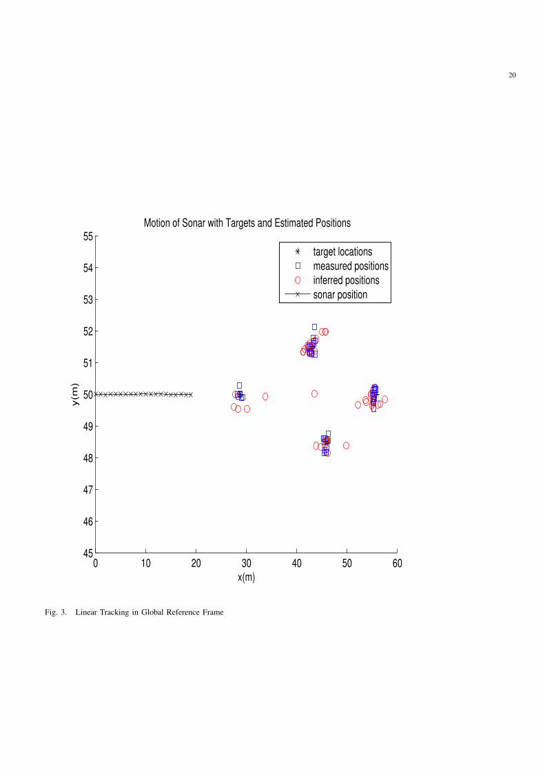
The results of the tracking for the simulated sonar run have been displayed in the sonar image reference frame

and the global reference frame. In the sonar image reference frame the objects are moving towards the sonar, figure

2 shows the measurements and estimated positions with respect to the sonar. In the global reference frame, figure

3, the sonar positions are marked on a global co-ordinate map and the objects are stationary. The actual positions

are shown along with the measurements and estimated positions. The tracker estimates well the number of targets

in each image which is between 1 and 4 targets. There are a few outliers where the position has wrongly estimated

a target location, this can often happen in the initialisation stage where the particles have been uniformly spread

and the distribution of particles are not sufficiently localised onto the target.

Obtaining accurate navigation information can be a significant problem during AUV missions. However, this

technique is still robust when no navigation information is present. The same scenario as above has been repeated

but the sequence of sonar images have been simulated with the AUV following a sinusoidal trajectory. The tracking

was then repeated with the system having no knowledge of the actual motion, and the results in the global reference

frame have been displayed in figure 4. The measurements taken were not as accurate as the linear path (figure 3)

but the tracker seems to perform well tracking the measurements with only a few false estimates.

B. Tracker on Real Data

The tracker was then applied to a sequence of real forward-look sonar images. The data was obtained from

a forward-looking sonar device fitted to an underwater vehicle where the sonar scans a sector of seabed in the

direction of the vehicle motion. The sequence of 18 images (figure 5) was obtained as the vehicle was flown towards

a cylindrical object lying on the seabed. The images are very noisy but the object can be seen in the sequence as

the small bright highlight moving from top right to bottom left in the sequence. The seabed over which the sonar

traverses appears to be composed of two different sediment types, one of which provided higher intensity returns.

This can be seen in the region before the target in the first 10 images of the sequence.

The results of the tracking is illustrated in figure 6. The measurements and tracked positions are in the sonar

reference frame, the global positions are unknown since no navigation information was provided with the data

14

and no accurate ground truth of the object’s location was available. The location of the cylinder is given by the

sequence of points from the lower right hand region of figure 6, moving towards the centre of the figure, as the

vehicle moves closer to the object. In the first few images, there were a lot of false targets, or clutter points, due to

bad observations of the cylinder as a result of high intensity returns from a region of seabed. These are the group

of measurements in the top half of figure 6.

To show how well the implementation works with clutter, the tracker has been run on the data forward in time

(where there are a lot of clutter points initially and fewer in the later images) and backward in time (where there are

few clutter points initially and more in the later images). This demonstration is to show how the initial conditions

affect the performance of the algorithm and the convergence as the clutter density at the start is different in this

sequence of images when run backward and forward. Running the algorithm in the forward direction results in

poor estimation initially but afterwards converges onto the correct target location (see figure 6). When the algorithm

is run on the data backwards, the algorithm quickly converges onto the correct target and manages to predict the

correct location through the clutter (see figure 7).

These results show that there is a sequence of images where there are few false alarms and then encounter a

cluttered region then the algorithm can predict the correct target but it works poorer if the cluttered region is at the

start. This can be expected as the distribution of the particles is propagated from one frame to the next and so if

the particles are predominantly located in the region of the true target they are more likely to track it well.

IV. DISCUSSION

An application of the particle PHD filter has been implemented for tracking a variable number of objects in a

sequence of forward-looking sonar images for the purpose of aligning data from a sequence of images to aid fusing

the data onto a global co-ordinate system where it will be reconstructed into a 3D map of the seabed.

The tracker was shown working on simulated data where the results could be displayed on a global map and

then on real sonar data with clutter for tracking a cylindrical object on the seabed. The simulated data provided a

test case scenario where accurate ground truth was available, but the simulated sonar images contain significantly

less noise and clutter than real data.

15

The current implementation tracks the objects in 2-dimensions, although it is currently being extended to 3D

forward looking sonar data.

This technique also has the capacity to incorporate measurements obtained from other sensing equipment such

as video data although the implementation here is restricted to sonar.

The identities of the objects are not determined in this implementation and so data association techniques are not

used. In many applications, knowledge of which target in the current frame relates to which target in the previous

frame is important and so the data association problem would need to be addressed. One of the advantages of the

PHD Filter is its ability to filter clutter and so the number of spurious measurements is reduced. Sonar data is very

noisy which gives rise to many spurious measurements and the PHD Filter copes well with this. If the identities

of the targets are needed then the data association problem is reduced although this needs to be addressed.

Future work will include addressing the data association issue for continuity of target identity and a comparison

of the PHD filter with the sample based JPDAF technique in cluttered data.

V. ACKNOWLEDGEMENTS

This work has been funded by QinetiQ through an MoD funded programme. The authors wish to express their

thanks to Dr. Douglas Carmichael and Dr. Samantha Dugelay from QinetiQ Bincleaves for their support and for

provision of sonar data. The authors would also like to thank Yvan Petillot and Yves de Saint-Pern in the Oceans

Lab at Heriot-Watt University for their help and useful comments.

REFERENCES

[1] S. Reed, I. Tena Ruiz, Y. Petillot, D. M. Lane, and J. M. Bell. Concurrent mapping and localisation using side-scan sonar for autonomous

navigation. Oceanic Engineering, IEEE Journal of, 29, Issue 2:442–456, 2004.

[2] Y. Petillot, I. Tena Ruiz, D. M. Lane, Y. Wang, E. Trucco, and N. Pican. Underwater vehicle path planning using a multi-beam forward

looking sonar. IEEE/OES OCEANS’98 conference, 1998.

[3] I. Tena Ruiz, Y. Petillot, and D. M. Lane. AUV navigation using a forward looking sonar. Unmanned Underwater Vehicle Symposium.

Rhode Island, USA., 2000.

[4] Y. Bar-Shalom and T.E. Fortmann. Tracking and Data Association. Academic Press, 1988.

[5] E. Trucco, Y. Petillot, I. Tena Ruiz, C. Plakas, and D. M. Lane. Feature tracking in video and sonar subsea sequences with applications.

Computer Vision and Image Understanding, No.79, pages 92–122.

16

[6] I. Tena Ruiz, D. M. Lane, and M. J. Chantler. A comparison of inter-frame feature measures for robust object classification in sector

scan sonar image sequences. IEEE Journal of Oceanic Engineering, 24, No.4:458–469, 1999.

[7] C. Hue, J.P. Le Cadre, and P. Perez. Tracking multiple objects with particle filtering. IEEE Trans. on Aerospace and Electronic Systems,

38(3):791–812, 2002.

[8] R. Karlsson and F. Gustafsson. Monte Carlo data association for multiple target tracking. Target Tracking: Algorithms and Applications

(Ref. No. 2001/174), IEE, 1:13/1– 13/5, 2001.

[9] M. Isard and J. MacCormick. Bramble: a Bayesian multiple-blob tracker. Computer Vision, 2001. ICCV 2001. Proceedings. Eighth

IEEE International Conference on, 2:34 – 41, 2001.

[10] C. Kreucher, K. Kastella, and A.O. Hero. A Bayesian method for integrated multitarget tracking and sensor management. Information

Fusion, 2003. Proceedings of the Sixth International Conference of ,Volume: 1 , July 8-11 2003, pages 704 – 711.

[11] People tracking with a mobile robot using sample-based Joint Probabilistic Data Association Filters. International Journal of Robotics

Research, pages 99–116, 2003.

[12] R. Mahler. Multitarget Bayes filtering via first-order multitarget moments. IEEE Transactions on Aerospace and Electronic Systems,

2003.

[13] H. Sidenbladh. Multi-target particle filtering for the Probability Hypothesis Density. International Conference on Information Fusion,

pages 800–806, 2003.

[14] B.N. Vo, S. Singh, and A. Doucet. Sequential Monte Carlo Implementation of the PHD filter for Multi-target Tracking. Proc. FUSION

2003, pages 792–799, 2003.

[15] T. Zajic and R. Mahler. A particle-systems implementation of the PHD multitarget tracking filter. SPIE Vol. 5096 Signal Processing,

Sensor Fusion and Target Recognition, pages 291–299, 2003.

[16] M. Tobias and A.D. Lanterman. A Probability Hypothesis Density-based multitarget tracker using multiple bistatic range and velocity

measurements. System Theory, 2004. Proceedings of the Thirty-Sixth Southeastern Symposium on , March 14-16, 2004, pages 205 –

209.

[17] D.L. Hall and J. Llinas, editors. Handbook of Multisensor Data Fusion, chapter 7. CRC Press, 2001.

[18] N.J. Gordon, D.J. Salmond, and A.F.M. Smith. Novel approach to nonlinear/non-Gaussian Bayesian state estimation. IEE Proceedings

on Radar and Signal Processing, 140:107–113, 1993.

[19] A. Doucet, N. de Freitas, and N. Gordon. Sequential Monte Carlo Methods in Practice. 2001.

[20] N. Gordon, D. Salmond, and C. Ewing. Bayesian State Estimation for Tracking and Guidance using the Bootstrap Filter. Journal of

Guidance, Control and Dynamics, 1995.

[21] J.M. Bell. A model for the Simulation of Side Scan Sonar. PhD thesis, Heriot-Watt University, 1995.

17

LIST OF FIGURES

1 Sequence of Simulated Forward Scan Sonar Images with Objects . . . . . . . . . . . . . . . . . . . . 18

2 Linear Tracking in Sonar Image Reference Frame . . . . . . . . . . . . . . . . . . . . . . . . . . . . 19

3 Linear Tracking in Global Reference Frame . . . . . . . . . . . . . . . . . . . . . . . . . . . . . . . . 20

4 Sinusoidal Sonar Tracking in Global Reference Frame . . . . . . . . . . . . . . . . . . . . . . . . . . 21

5 Sequence of Real Forward-Scan Images . . . . . . . . . . . . . . . . . . . . . . . . . . . . . . . . . . 22

6 Tracked Cylinder in Forward Direction . . . . . . . . . . . . . . . . . . . . . . . . . . . . . . . . . . 23

7 Tracked Cylinder in Backward Direction . . . . . . . . . . . . . . . . . . . . . . . . . . . . . . . . . 24

18

Fig. 1. Sequence of Simulated Forward Scan Sonar Images with Objects

19

0 10 20 30 40 50 60−2.5

−2

−1.5

−1

−0.5

0

0.5

1

1.5

2

2.5

x(m)

y(m

)

Measurements and Estimated Positions in Sonar Reference Frame

measured positionsinferred positionsobserver position

Fig. 2. Linear Tracking in Sonar Image Reference Frame

20

0 10 20 30 40 50 6045

46

47

48

49

50

51

52

53

54

55

x(m)

y(m

)

Motion of Sonar with Targets and Estimated Positions

target locationsmeasured positionsinferred positionssonar position

Fig. 3. Linear Tracking in Global Reference Frame

21

0 10 20 30 40 50 6045

46

47

48

49

50

51

52

53

54

55

x(m)

y(m

)

Motion of Sonar with Targets and Estimated Positions

target locationsmeasured positionsinferred positionssonar position

Fig. 4. Sinusoidal Sonar Tracking in Global Reference Frame

22

Fig. 5. Sequence of Real Forward-Scan Images

23

0 10 20 30 40 50 60 70 80−8

−6

−4

−2

0

2

4

6

x(m)

y(m

)

PHD Tracking Example on Real Sonar Data

measured positionsinferred positionsobserver position

Fig. 6. Tracked Cylinder in Forward Direction

24

0 10 20 30 40 50 60 70 80−10

−5

0

5

x(m)

y(m

)

PHD Tracking Example on Real Sonar Data

measured positionsinferred positionsobserver position

Fig. 7. Tracked Cylinder in Backward Direction