1 Bayesian Decision Theory Z. Ghassabi. 2 Outline What is pattern recognition? What is classification? Need for Probabilistic Reasoning Probabilistic

1

Bayesian Decision Theory

Z. Ghassabi

2

Outline

What is pattern recognition? What is classification?

Need for Probabilistic Reasoning Probabilistic Classification Theory

What is Bayesian Decision Theory? HISTORY PRIOR PROBABILITIES CLASS-CONDITIONAL PROBABILITIES BAYES FORMULA A Casual Formulation Decision

3

Outline

What is Bayesian Decision Theory? Decision fot Two Categories

4

Outline

What is classification? Classification by Bayesian

Classification Basic Concepts Bayes Rule More General Forms of Bayes Rule Discriminated Functions Bayesian Belief Networks

5

TYPICAL APPLICATIONS OF PRIMAGE PROCESSING EXAMPLE

• Sorting Fish: incoming fish are sorted according to species using optical sensing (sea bass or salmon?)

Feature Extraction

Segmentation

Sensing

• Problem Analysis:

set up a camera and take some sample images to extract features

Consider features such as length, lightness, width, number and shape of fins, position of mouth, etc.

What is pattern recognition?

6

Preprocessing Segment (isolate) fishes from one another

and from the background Feature Extraction

Reduce the data by measuring certain features

Classification Divide the feature space into decision regions

Pattern Classification System

7

8

Initially use the length of the fish as a possible feature for discrimination

Classification

9

TYPICAL APPLICATIONS

LENGTH AS A DISCRIMINATOR

• Length is a poor discriminator

10

The length is a poor feature alone!

Select the lightness as a possible feature

Feature Selection

11

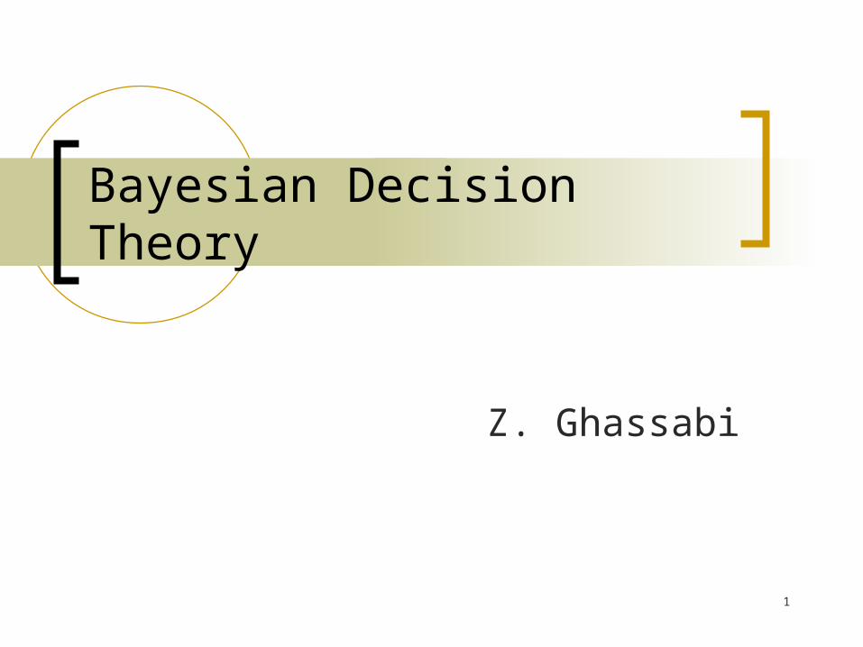
TYPICAL APPLICATIONSADD ANOTHER FEATURE

• Lightness is a better feature than length because it reduces the misclassification error.

• Can we combine features in such a way that we improve performance? (Hint: correlation)

12

Move decision boundary toward smaller values of lightness in order to minimize the cost (reduce the number of sea bass that are classified salmon!)

Task of decision theory

Threshold decision boundary and cost relationship

13

Adopt the lightness and add the width of the fish to the feature vector

Fish xT = [x1, x2]

Lightness Width

Feature Vector

14

TYPICAL APPLICATIONSWIDTH AND LIGHTNESS

• Treat features as a N-tuple (two-dimensional vector)

• Create a scatter plot

• Draw a line (regression) separating the two classes

Straight line decision boundary

15

We might add other features that are not highly correlated with the ones we already have. Be sure not to reduce the performance by adding “noisy features”

Ideally, you might think the best decision boundary is the one that provides optimal performance on the training data (see the following figure)

Features

16

TYPICAL APPLICATIONSDECISION THEORY

• Can we do better than a linear classifier?

• What is wrong with this decision surface? (hint: generalization)

Is this a good decision boundary?

17

Our satisfaction is premature because the central aim of designing a classifier is to correctly classify new (test) input

Issue of generalization!

Decision Boundary Choice

18

TYPICAL APPLICATIONSGENERALIZATION AND RISK

• Why might a smoother decision surface be a better choice? (hint: Occam’s Razor).

• PR investigates how to find such “optimal” decision surfaces and how to provide system designers with the tools to make intelligent trade-offs.

Better decision boundary

19

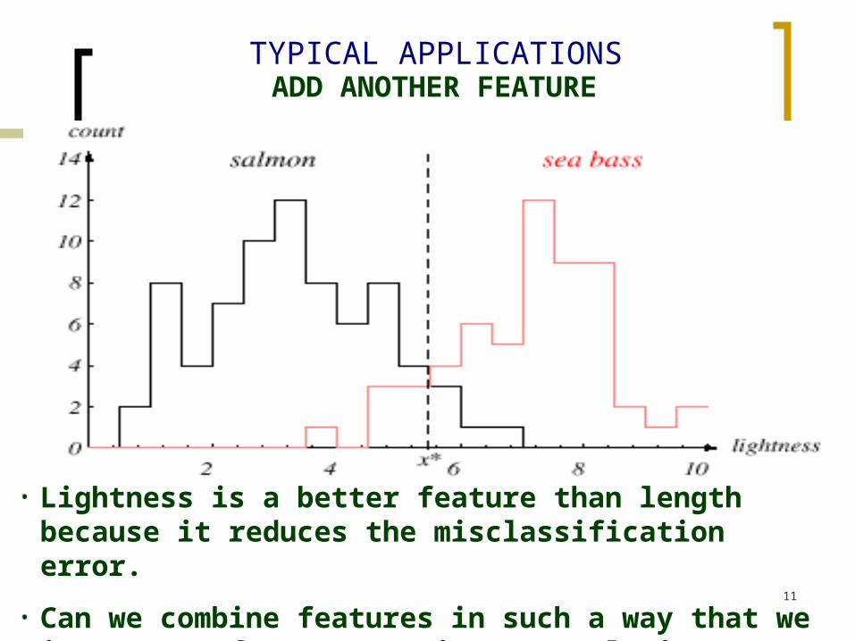
Need for Probabilistic Reasoning

Most everyday reasoning is based on uncertain evidence and inferences.

Classical logic, which only allows conclusions to be strictly true or strictly false, does not account for this uncertainty or the need to weigh and combine conflicting evidence.

Todays expert systems employed fairly ad hoc methods for reasoning under uncertainty and for combining evidence.

20

Probabilistic Classification Theory

درclassification ،کالسها با هم همپوشانی دارند بنابراین هر الگو با یک احتمالی به یک کالس متعلق

است. In practice, some overlap between classes and

random variation within classes occur, hence perfect separation between classes can not be achieved: Misclassification may occur.

تئوریBayesian decision اجازه می دهد تا تابع هزینه ای ارائه شود برای موقعی که ممکن است که یک

است اشتباها به Aبردار ورودی که عضوی از کالس (misclassify) نسبت داده شود. Bکالس

21

HISTORY

Bayesian Probability was named after Reverend Thomas Bayes (1702-1761).

He proved a special case of what is currently known as the Bayes Theorem.

The term “Bayesian” came into use around the 1950’s.

http://en.wikipedia.org/wiki/Bayesian_probabilityhttp://en.wikipedia.org/wiki/Bayesian_probability

What is Bayesian Decision Theory?

22

HISTORY (Cont.) Pierre-Simon, Marquis de Laplace (1749-

1827) independently proved a generalized version of Bayes Theorem.

1970 Bayesian Belief Network at Stanford University (Judea Pearl 1988)

The idea’s proposed above was not fully developed until later. BBN became popular in the 1990s.

23

HISTORY (Cont.)

Current uses of Bayesian Networks: Microsoft’s printer troubleshooter. Diagnose diseases (Mycin). Used to predict oil and stock prices Control the space shuttle Risk Analysis – Schedule and Cost Overruns.

24

Bayesian decision theory is a fundamental statistical approach to the problem of pattern classification.

Using probabilistic approach to help making decision (e.g., classification) so as to minimize the risk (cost).

Assume all relevant probability distributions are known (later we will learn how to estimate these from data).

BAYESIAN DECISION THEORYPROBABILISTIC DECISION THEORY

25

State of nature is prior information

denote the state of nature

Model as a random variable, :

= 1: the event that the next fish is a sea bass

category 1: sea bass; category 2: salmon• A priori probabilities:

P(1) = probability of category 1

P(2) = probability of category 2

P(1) + P( 2) = 1 (either 1 or 2 must occur)

• Decision rule Decide 1 if P(1) > P(2); otherwise, decide 2

BAYESIAN DECISION THEORYPRIOR PROBABILITIES

But we know there will be many mistakes.…

http://www.stat.yale.edu/Courses/1997-98/101/ranvar.htm

26

BAYESIAN DECISION THEORYCLASS-CONDITIONAL PROBABILITIES

A decision rule with only prior information always produces the same result and ignores measurements.

If P(1) >> P( 2), we will be correct most of the time.

• Given a feature, x (lightness), which is a continuous random variable, p(x|2) is the class-conditional probability density function:

• p(x|1) and p(x|2) describe the difference in lightness between populations of sea and salmon.

27

p(lightness | salmon) ?

P(lightness | sea bass) ?

Let x be a continuous random variable .p(x|w) is the probability density for x given the state of nature w.

28

Suppose we know both P(j) and p(x|j), and we can

measure x. How does this influence our decision?

The joint probability that of finding a pattern that is in

category j and that this pattern has a feature value of x is:

BAYESIAN DECISION THEORYBAYES FORMULA

jjjj PxpxpxP)x,(p

• Rearranging terms, we arrive at Bayes formula.

How do we combine a priori and class-conditional probabilities to know the probability of a state of nature?

29

Bayes formula:

can be expressed in words as:

By measuring x, we can convert the prior probability,

P(j), into a posterior probability, P(j|x).

Evidence can be viewed as a scale factor and is often

ignored in optimization applications (e.g., speech

recognition).

BAYESIAN DECISION THEORYPOSTERIOR PROBABILITIES

xp

PxpxP

jjj

evidencepriorlikelihood

posterior

Bayes Decision:Choose w1 if P(w1|x) > P(w2|x); otherwise choose w2.

For two categories:

A Casual Formulation•The prior probability reflects knowledge of the relative frequency of instances of a class•The likelihood is a measure of the probability that a measurement value occurs in a class•The evidence is a scaling term

30

BAYESIAN THEOREM

A special case of Bayesian Theorem:

P(A∩B) = P(B) x P(A|B)

P(B∩A) = P(A) x P(B|A)

Since P(A∩B) = P(B∩A),

P(B) x P(A|B) = P(A) x P(B|A)

=> P(A|B) = [P(A) x P(B|A)] / P(B)

A B

ABPAPABPAP

ABPAP

BP

ABPAPBAP

||

)|()(

)(

)|()()|(

31

Preliminaries and Notations

:},,,{ 21 ci a state of nature

:)( iP prior probability

:x feature vector

:)|( ip x class-conditionaldensity

:)|( xiP posterior probability

32

Decision )(

)()|()|(

x

xx

p

PpP ii

i

( ) arg max ( | )i

iP

x xD( ) arg max ( | )i

iP

x xD

Decide i if P(i|x) > P(j|x) j i

Decide i if p(x|i)P(i) > p(x|j)P(j) j i

Special cases:1. P(1)=P(2)= =P(c)2. p(x|1)=p(x|2) = = p(x|c)

x gives us no useful information

decision is based entirely on the likelihood, p(x|j).

The evidence, p(x), is a scale factor that assures conditional probabilities sum to 1: P(1|x)+P(2|x)=1

We can eliminate the scale factor (which appears on both sides of the equation):

33

Two Categories

Decide i if P(i|x) > P(j|x) j i

Decide i if p(x|i)P(i) > p(x|j)P(j) j i

Decide 1 if P(1|x) > P(2|x); otherwise decide 2

Decide 1 if p(x|1)P(1) > p(x|2)P(2); otherwise decide 2

Special cases:1. P(1)=P(2)

Decide 1 if p(x|1) > p(x|2); otherwise decide 2

2. p(x|1)=p(x|2)Decide 1 if P(1) > P(2); otherwise decide 2

34

Example

R2

P(1)=P(2)

R1


Decide 1 if p(x|> p(x|2); otherwise decide 1



Decide 1 if p(x|> p(x|2); otherwise decide 1


35

Example

R1R1

R2

R2

P(1)=2/3P(2)=1/3

Decide 1 if p(x|1)P(1) > p(x|2)P(2); otherwise decide 2

Bayes Decision Rule

36

BAYESIAN DECISION THEORYPOSTERIOR PROBABILITIES

For every value of x, the posteriors sum to 1.0.

At x=14, the probability it is in category 2 is 0.08, and for

category 1 is 0.92.

Two-class fish sorting problem (P(1) = 2/3, P(2) = 1/3):

37

Classification Error Decision rule:

For an observation x, decide 1 if P(1|x) > P(2|x); otherwise, decide 2

Probability of error:

The average probability of error is given by:

If for every x we ensure that P(error|x) is as small as possible,

then the integral is as small as possible. Thus, Bayes decision

rule for minimizes P(error).

BAYESIAN DECISION THEORYBAYES DECISION RULE

21

12

x)x(P

x)x(Px|errorP

dx)x(p)x|error(Pdx)x,error(P)error(P

)]x(P),x(Pmin[)x|error(P 21 Consider two categories:

38

Generalization of the preceding ideas: Use of more than one feature

(e.g., length and lightness) Use more than two states of nature

(e.g., N-way classification) Allowing actions other than a decision to decide on the state

of nature (e.g., rejection: refusing to take an action when alternatives are close or confidence is low)

Introduce a loss of function which is more general than the probability of error(e.g., errors are not equally costly)

Let us replace the scalar x by the vector x in a d-dimensional Euclidean space, Rd, calledthe feature space.

CONTINUOUS FEATURES

GENERALIZATION OF TWO-CLASS PROBLEM

39

The Generation

:},,,{ 21 c a set of c states of nature or c categories

:},,,{ 21 a a set of a possible actions

:)|( jiij The loss incurred for taking action i when the true state of nature is j.

We want to minimize the expected loss in making decision.

Risk

can be zero.

LOSS FUNCTION

40

Examples

Ex 1: Fish classification X= is the image of fish x =(brightness, length, fin

#, etc.) is our belief what the fish

type is = {“sea bass”, “salmon”,

“trout”, etc} is a decision for the

fish type, in this case = {“sea bass”, “salmon”,

“trout”, “manual expection needed”, etc}

Ex 2: Medical diagnosis X= all the available medical

tests, imaging scans that a doctor can order for a patient

x =(blood pressure, glucose level, cough, x-ray, etc.)

is an illness type ={“Flu”, “cold”, “TB”,

“pneumonia”, “lung cancer”, etc}

is a decision for treatment, = {“Tylenol”, “Hospitalize”,

“more tests needed”, etc}

C

C

41

Conditional Risk

c

jjjii PR

1

)|()|()|( xx

c

jjij P

1

)|( x

Given x, the expected loss (risk)

associated with taking action i.

Given x, the expected loss (risk)

associated with taking action i.

)(

)()|()|(

x

xx

p

PpP jj

j

)()|()(1

j

c

jj Ppp

xx

42

0/1 Loss Function

otherwise1

with assiciateddecision correct a is 0)|( ji

ji

c

jjjii PR

1

)|()|()|( xx

c

jjij P

1

)|( x

( | ) ( | )iR P error x x

21

12

x)x(P

x)x(Px|errorP

43

Decision

c

jjjii PR

1

)|()|()|( xx

c

jjij P

1

)|( x

)|(minarg)( xx iRi

)|(minarg)( xx iRi

Bayesian Decision Rule:

A general decision rule is a function (x) that tells us which action to take for every possible observation.

44

Overall Risk

xxxx dpRR )()|)((Decision function

Bayesian decision rule:

the optimal one to minimize the overall riskIts resulting overall risk is called the Bayesian risk

)|(minarg)( xx iRi

)|(minarg)( xx iRi

The overall risk is given by:

If we choose (x) so that R(i(x)) is as small as possible for every x, the overall risk will be minimized.

Compute the conditional risk for every and select the action that minimizes R(i|x). This is denoted R*, and is referred to as the Bayes risk

The Bayes risk is the best performance that can be achieved.

45

Two-Category Classification

},{ 21

},{ 21 A

ctio

n

State of Nature

1 2

1 11 12

2 21 22

Loss Function

)|()|()|( 2121111 xxx PPR

)|()|()|( 2221212 xxx PPR

Let 1 correspond to 1, 2 to 2, and ij = (i|j)

The conditional risk is given by:

46


)|()|()|( 2121111 xxx PPR

)|()|()|( 2221212 xxx PPR

Perform 1 if R(2|x) > R(1|x); otherwise perform 2

)|()|()|()|( 212111222121 xxxx PPPP

)|()()|()( 2221211121 xx PP

Our decision rule is:choose 1 if: R(1|x) < R(2|x);otherwise decide 2

47



)|()|()|()|( 212111222121 xxxx PPPP

positive

)|()()|()( 2221211121 xx PP

positive

Posterior probabilities are scaled before comparison.

If the loss incurred for making an error is greater than that incurred for being correct, the factors (21- 11) and(12- 22) are positive, and the ratio of these factors simply scales the posteriors.

48

Two-Category Classification)(

)()|()|(

x

xx

p

PpP ii

i

irrelevan

t

irrelevant


)|()|()|()|( 212111222121 xxxx PPPP

)|()()|()( 2221211121 xx PP

)()|()()()|()( 222212111121 PpPp xx

)(

)(

)(

)(

)|(

)|(

1

2

1121

2212

2

1

P

P

p

p

x

x

By employing Bayes formula, we can replace the posteriors by the prior probabilities and conditional densities:

49


)(

)(

)(

)(

)|(

)|(

1

2

1121

2212

2

1

P

P

p

p

x

xPerform 1 if

LikelihoodRatio

Threshold

This slide will be recalled later.This slide will be recalled later.

Stated as:

Choose a1 if the likelihood ration exceeds a threshold value independent of the observation x.

50

51

Loss Factors

0 1

1 0

1 0

0 1

1 1

1 1

1 1

0 0

1 0

1 0

If the loss factors are identical, and the prior probabilities are equal, this reduces to a standard likelihood ratio:

12

11

)|(p)|(p

:ifchoosexx

52

Consider a symmetrical or zero-one loss function:

c,...,,j,iji

ji)( ji 21

1

0

MINIMUM ERROR RATE

The conditional risk is:

x(

x(

x(x

j

jj

i

c

ij

c

jii

(P

(P

(P)(R)(R

1

1

The conditional risk is the average probability of error.

To minimize error, maximize P(i|x) — also known as maximum a posteriori decoding (MAP).

Error rate (the probability of error) is to be minimizedError rate (the probability of error) is to be minimized

53

Minimum Error RateLIKELIHOOD RATIO

Minimum error rate classification:

choose i if: P(i| x) > P(j| x) for all ji

54

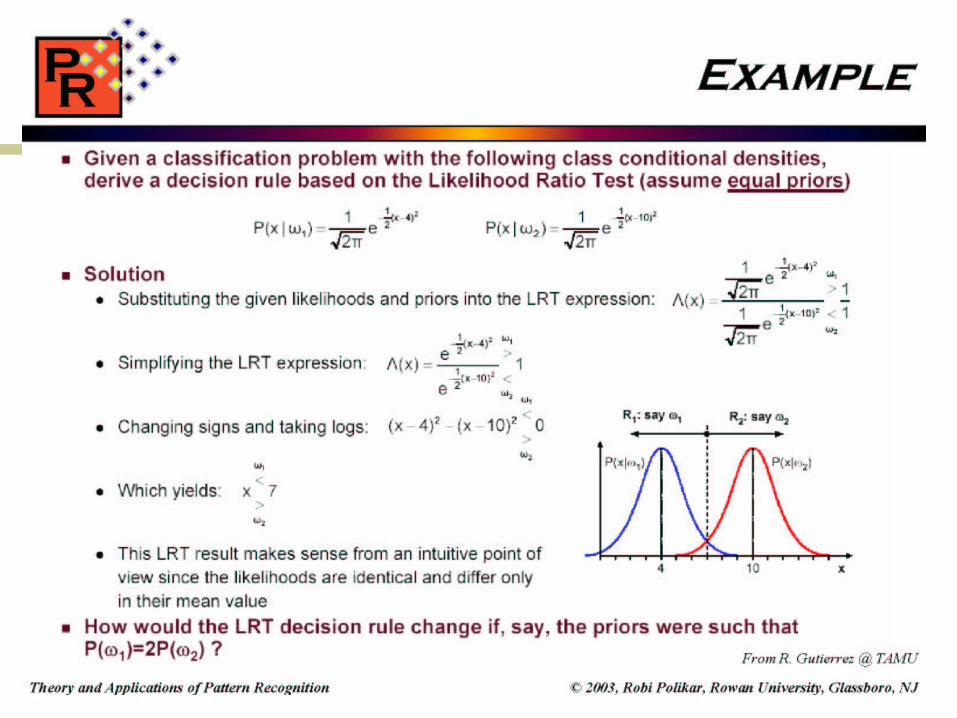
Example

For sea bass population, the lightness x is a normal random variable distributes according to N(4,1);

for salmon population x is distributed according to N(10,1);

Select the optimal decision where:

a. The two fish are equiprobable

b. P(sea bass) = 2X P(salmon)

c. The cost of classifying a fish as a salmon when it truly is seabass is 2$, and t The cost of classifying a fish as a seabass when it is truly a salmon is 1$.

2

55

56

57

End of Section 1

58

59

The Multicategory Classification

g1(x)g1(x)

g2(x)g2(x)

gc(x)gc(x)

x Action(e.g., classification)

(x)

The classifier Assign x to i ifgi(x) > gj(x) for all j i.

gi(x)’s are called the discriminant functions.

How to define discriminant functions?

How do we represent pattern classifiers?

The most common way is through discriminant functions.Remember we use {w1,w2, …, wc} to be the possible states of nature.

For each class we create a discriminant function gi(x).

Our classifier is a network or machine that computes c discriminant functions.

60

Simple Discriminant Functions

)|()( xx ii Rg

)|()( xx ii Pg

Minimum Risk case:

Minimum Error-Rate case:

)()|()( iii Ppg xx

)(ln)|(ln)( iii Ppg xx

If f( ． ) is a monotonically increasing function, than f(gi( ． ) )’s are also be discriminant functions.

Notice the decision is the same if we change every gi(x) for f(gi(x)) Assuming f(.) is a monotonically increasing function.

61

Figure 2.5

62

Decision Regions

} )()(|{ ijgg jii xxxR

Two-category example

Decision regions are separated by decision boundaries.

The net effect is to divide the feature space into c regions (one for each class). We then have c decision regions separated by decision boundaries.

63

Figure 2.6

64

Bayesian Decision Theory(Classification)

The Normal Distribution

65

Basics of Probability

Discrete random variable (X) － Assume integer

Continuous random variable (X)

Probability mass function (pmf): )()( xXPxp

Cumulative distribution function (cdf):

x

t

tpxXPxF )()()(

Probability density function (pdf): )(or )( xfxp

Cumulative distribution function (cdf):

xdttpxXPxF )()()(

not a probability

66

Probability mass function

•The graph of a probability mass function. •All the values of this function must be non-negative and sum up to 1.

67

Probability density function The pdf can be calculated by taking the integral of

the function f(x) by the integration interval of the input variable x.

For example: the probability of the variable X being within the interval [4.3,7.8] would be

68

Expectations

continuous is )()(

discrete is )()()]([

Xdxxpxg

XxpxgXgE x

continuous is )()(

discrete is )()()]([

Xdxxpxg

XxpxgXgE x

Let g be a function of random variable X.

The kth moment ][ kXE

The kth central moments ])[( kXXE

The 1st moment ][XEX

69

Important Expectations

Mean

continuous is )(

discrete is )(][

Xdxxxp

XxxpXE xX

Variance

continuous is )()(

discrete is )()(])[(][

2

2

22

Xdxxpx

XxpxXEXVar

X

xX

XX

Fact: 22 ])[(][][ XEXEXVar 22 ])[(][][ XEXEXVar

70

Entropy

continuous is )(ln)(

discrete is )(ln)(][

Xdxxpxp

XxpxpXH x

continuous is )(ln)(

discrete is )(ln)(][

Xdxxpxp

XxpxpXH x

The entropy measures the fundamental uncertainty in the value of points selected randomly from a distribution.

71

Univariate Gaussian Distribution

x

p(x)X~N(μ,σ2)

2

2

2

)(

2

1)(

x

exp2

2

2

)(

2

1)(

x

exp μ

σ σ

2σ 2σ

3σ 3σE[X] =μ

Var[X] =σ2

Properties:1. Maximize the entropy2. Central limit theorem

72

Illustration of the central limit theorem Let x1,x2,…,xn be a sequence of n independent and identically distributed random variables having each finite values of expectation µ and variance σ2>0 The central limit theorem states that as the sample size n increases, the distribution of the sample average of these random variables approaches the normal distribution with a mean µ and variance σ2 / n irrespective of the shape of the original distribution.

Original probability density function

A probability density function

Probability density function of the sum of two terms

Probability density function of the sum of three terms

Probability density function of the sum of four terms

73

Random Vectors

dR:XdR:XA d-dimensional

random vector

TdE ),,,(][ 21 XμVector Mean:

Covariance Matrix:

]))([( TE μXμXΣ

221

22221

11221

ddd

d

d

TdXXX ),,,( 21 X

74

Multivariate Gaussian Distribution

X~N(μ,Σ)

)()(

2

1exp

||)2(

1)( 1

2/12/μxΣμx

Σx T

dp

)()(

2

1exp

||)2(

1)( 1

2/12/μxΣμx

Σx T

dp

E[X] =μ

E[(X-μ) (X-μ)T] =Σ

2

2

2

)(

2

1)(

x

exp2

2

2

)(

2

1)(

x

exp

A d-dimensional random vector

75

Properties of N(μ,Σ)

X~N(μ,Σ) A d-dimensional random vector

Let Y=ATX, where A is a d × k matrix.

Y~N(ATμ, ATΣA)

76

Properties of N(μ,Σ)

X~N(μ,Σ) A d-dimensional random vector

Let Y=ATX, where A is a d × k matrix.

Y~N(ATμ, ATΣA)

77

On Parameters of N(μ,Σ)

X~N(μ,Σ) TdXXX ),,,( 21 X

TdE ),,,(][ 21 Xμ

ddijTE ][]))([( μXμXΣ

][ ii XE ][ ii XE

),()])([( jijjiiij XXCovXXE ),()])([( jijjiiij XXCovXXE

)(])[( 22iiiiii XVarXE )(])[( 22

iiiiii XVarXE

0 ijji XX

78

More On Covariance Matrix

ddijTE ][]))([( μXμXΣ

),()])([( jijjiiij XXCovXXE ),()])([( jijjiiij XXCovXXE

)(])[( 22iiiiii XVarXE )(])[( 22

iiiiii XVarXE

0 ijji XX

is symmetric and positive semidefinite.TΦΛΦΣ

: orthonormal matrix, whose columns are eigenvectors of . : diagonal matrix (eigenvalues).

TΦΛΦΛ 2/12/1

T))(( 2/12/1 ΦΛΦΛΣ T))(( 2/12/1 ΦΛΦΛΣ

79

Whitening Transform

X~N(μ,Σ)

Y=ATX Y~N(ATμ, ATΣA)

T))(( 2/12/1 ΦΛΦΛΣ T))(( 2/12/1 ΦΛΦΛΣ

Let 2/1ΦΛwA2/1ΦΛwA

),(~ wTw

Tww NX ΣAAμAA

IΦΛΦΛΦΛΦΛΣAA )())(()( 2/12/12/12/1 TTw

Tw

),(~ IμAA Tww NX ),(~ IμAA T

ww NX

80

Whitening Transform

X~N(μ,Σ)

Y=ATX Y~N(ATμ, ATΣA)

T))(( 2/12/1 ΦΛΦΛΣ T))(( 2/12/1 ΦΛΦΛΣ

Let 2/1ΦΛwA2/1ΦΛwA

),(~ wTw

Tww NX ΣAAμAA

IΦΛΦΛΦΛΦΛΣAA )())(()( 2/12/12/12/1 TTw

Tw

),(~ IμAA Tww NX ),(~ IμAA T

ww NX

Whitening

Projection

LinearTransform

81

Whitening Transform•The whitening transformation is a decorrelation method that converts the covariance matrix S of a set of samples into the identity matrix I. •This effectively creates new random variables that are uncorrelated and have the same variances as the original random variables. •The method is called the whitening transform because it transforms the input matrix closer towards white noise.

This can be expressed as 2/1ΦΛwA2/1ΦΛwA

where Φ is the matrix with the eigenvectors of "S" as its columns and Λ is the diagonal matrix of non-increasing eigenvalues.

82

White noise

•White noise is a random signal (or process) with a flat power spectral density. •In other words, the signal contains equal power within a fixed bandwidth at any center frequency.

Energy spectral density

83

Mahalanobis Distance

)()(

2

1exp

||)2(

1)( 1

2/12/μxΣμx

Σx T

dp

)()(

2

1exp

||)2(

1)( 1

2/12/μxΣμx

Σx T

dp

constant

)()( 12 μxΣμx Tr )()( 12 μxΣμx Tr

r2depends on the value of r2

X~N(μ,Σ)

84

Mahalanobis distance In statistics, Mahalanobis distance is a distance measure introduced by P. C. Mahalanobis in 1936.It is based on correlations between variables by which different patternscan be identified and analyzed.It is a useful way of determining similarity of an unknown sample set to aknown one. It differs from Euclidean distance in that it takes into account the correlations of the data set and is scale-invariant, i.e. not dependent on the scale of measurements .

85

Mahalanobis distance Formally, the Mahalanobis distance from a group of values

with above mean and covariance matrix Σ for a multivariate vector is defined as:

Mahalanobis distance can also be defined as dissimilarity measure between two random vectors of the same distribution with the covariance matrix Σ :

If the covariance matrix is the identity matrix, the Mahalanobis distance reduces to the Euclidean distance. If the covariance matrix is diagonal, then the resulting distance measure is called the normalized Euclidean distance:

where σi is the standard deviation of the xi over the sample set.

86

Mahalanobis Distance

)()(

2

1exp

||)2(

1)( 1

2/12/μxΣμx

Σx T

dp

)()(

2

1exp

||)2(

1)( 1

2/12/μxΣμx

Σx T

dp

constant

)()( 12 μxΣμx Tr )()( 12 μxΣμx Tr

r2depends on the value of r2

X~N(μ,Σ)

87


Discriminant Functions for the Normal Populations

88

Normal Density

If features are statistically independent and the variance is the samefor all features, the discriminant function is simple and is linear in nature.

A classifier that uses linear discriminant functions is called a linear machine.

The decision surface are pieces of hyperplanes defined by linear equations.

89

Minimum-Error-Rate Classification

)|()( xx ii Pg )()|()( iii Ppg xx

)(ln)|(ln)( iii Ppg xx

Xi~N(μi,Σi)

)()(

2

1exp

||)2(

1)|( 1

2/12/ iiT

ii

dip μxΣμxΣ

x

)()(

2

1exp

||)2(

1)|( 1

2/12/ iiT

ii

dip μxΣμxΣ

x

)(ln||ln2

12ln

2)()(

2

1)( 1

iiiiT

ii Pd

g ΣμxΣμxx )(ln||ln2

12ln

2)()(

2

1)( 1

iiiiT

ii Pd

g ΣμxΣμxx

Assuming the measurements are normally distributed, we have

90

Some Algebra to Simplify the Discriminants

Since

We take the natural logarithm to re-write the first term

)(ln)|(ln)( iii Pxpxg

)()(2

1

2/12/

)()(2

1

2/12/

1

1

ln||2

1ln

||2

1ln|ln

iit

i

iit

i

xx

id

xx

idi

e

e)p(x

91

Some Algebra to Simplify the Discriminants (continued)

||ln2

12ln

2)()(

2

1

||ln2ln)()(2

1

||2ln)()(2

1

ln||2

1ln

1

2/12/1

2/12/1

)()(2

1

2/12/

1

iiit

i

id

iit

i

id

iit

i

xx

id

dxx

xx

xx

eii

ti

92


)(ln||ln2

12ln

2)()(

2

1)( 1

iiiiT

ii Pd


12ln

2)()(

2

1)( 1

iiiiT

ii Pd

g ΣμxΣμxx

Three Cases:Case 1: IΣ 2i

Case 2: ΣΣ i

Case 3: ji ΣΣ

Classes are centered at different mean, and their feature components are pairwisely independent have the same variance.

Classes are centered at different mean, but have the same variation.

Arbitrary.

93

Case 1. i = 2I

di

2

2

2

2

...00

.........0

0...0

000

i oft independen is2Ii

omitted bemay and i oft independen is 2ln2

d

)(ln||ln2

12ln

2)()(

2

1)( 1

iiiiT

ii Pd


12ln

2)()(

2

1)( 1

iiiiT

ii Pd

g ΣμxΣμxx

irrelevant

)(ln||||2

1)( 2

2 iii Pg

μxx

IΣ2

1 1

iIΣ

21 1

i

)(ln)2(2

12 ii

Ti

Ti

T P

μμxμxx

irrelevant

)(ln

2

11)(

22 iiTi

Tii Pg

μμxμx

toreduced becan )( constant), (a || Since 2 xgid

i

so omitted bemay and i oft independen is but xxt

94

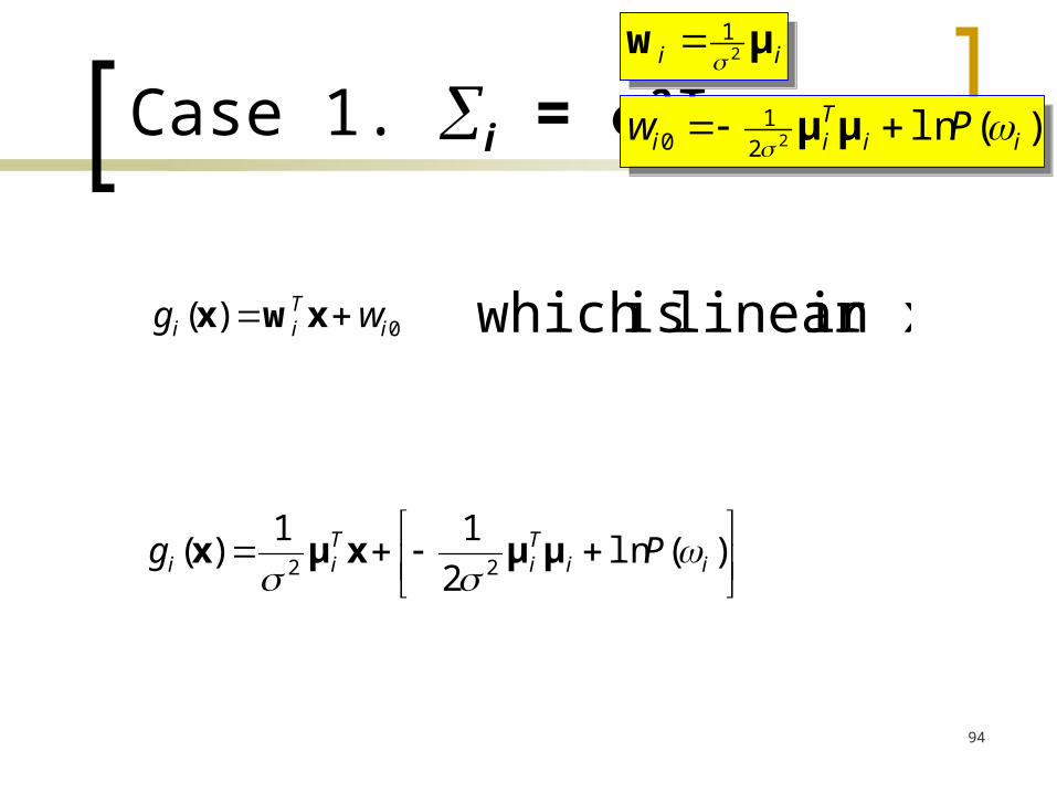
Case 1. i = 2Iii μw 2

1

ii μw 21

)(ln

2

11)(

22 iiTi

Tii Pg

μμxμx

)(ln221

0 iiTii Pw

μμ )(ln22

10 ii

Tii Pw

μμ

0)( iTii wg xwx in x!linear iswhich

95

Case 1. i = 2Iii μw 2

1

ii μw 21

)(ln221

0 iiTii Pw

μμ )(ln22

10 ii

Tii Pw

μμ

0)( iTii wg xwx

i j

Boundary btw. i and j

)()( xx ji gg 00 j

Tji

Ti ww xwxw

00)( ijTj

Ti ww xww

)(

)(ln)()( 2

21

j

ij

Tji

Ti

Tj

Ti P

P

μμμμxμμ

)(

)(ln

||||

))(())(()(

22

21

j

i

ji

jiTj

Ti

jiTj

Ti

Tj

Ti P

P

μμ

μμμμμμμμxμμ

96

Case 1. i = 2I

i j

Boundary btw. i and j

)()( xx ji gg

)(

)(ln

||||

))(())(()(

22

21

j

i

ji

jiTj

Ti

jiTj

Ti

Tj

Ti P

P

μμ

μμμμμμμμxμμ

wT

w0)( 0 xxwT

)()(

)(ln

||||)(

2

2

21

0 jij

i

jiji P

Pμμ

μμμμx

ji μμw x0

x

xx0

The decision boundary will be a hyperplane perpendicular to the line btw. the means at somewhere.

0 if P( i)=P( j)midpoint

97

Case 1. i = 2I)(

)(

)(ln

||||)( 21

2

12

21

2

2121

0 μμμμ

μμx

P

P

)()( 21 PP

Minimum distance classifier (template matching)

The decision region when the priors are equal and the support regions are spherical is simply halfway between the means (Euclidean distance).

98

99

Case 1. i = 2I

)()( 21 PP

)()(

)(ln

||||)( 21

2

12

21

2

2121

0 μμμμ

μμx

P

P

Note how priors shift the boundary away from the more likely mean !!!

100

Case 1. i = 2I

)()( 21 PP

)()(

)(ln

||||)( 21

2

12

21

2

2121

0 μμμμ

μμx

P

P

101

Case 1. i = 2I

)()( 21 PP

)()(

)(ln

||||)( 21

2

12

21

2

2121

0 μμμμ

μμx

P

P

102

Case 2. i =

)(ln||ln2

12ln

2)()(

2

1)( 1

iiiiT

ii Pd


12ln

2)()(

2

1)( 1

iiiiT

ii Pd

g ΣμxΣμxx

Irrelevant ifP( i)= P( j) i, j

)(ln)()(2

1)( 1

iiT

ii Pg μxΣμxx

MahalanobisDistance

irrelevant

•Covariance matrices are arbitrary, but equal to each other for all classes.• Features then form hyper-ellipsoidal clusters of equal size and shape.

103

Case 2. i =

)(ln)()(2

1)( 1

iiT

ii Pg μxΣμxx

)(ln)2(2

1 111ii

Ti

Ti

T P μΣμxΣμxΣx

Irrelevant

0)( iTii wg xwx

ii μΣw 1 ii μΣw 1

)(ln121

0 iiTii Pw μΣμ )(ln1

21

0 iiTii Pw μΣμ

104

Case 2. i =

0)( iTii wg xwx

ii μΣw 1 ii μΣw 1

)(ln121

0 iiTii Pw μΣμ )(ln1

21

0 iiTii Pw μΣμ

i j

)()( xx ji gg 0)( 0 xxwT

)(1ji μμΣw

)()()(

)](/)(ln[)(

121

0 jiji

Tji

jiji

PPμμ

μμΣμμμμx

w

x0

xThe discriminant hyperplanes are often not

orthogonal to the segments joining the class means

105

Case 2. i =

106

Case 2. i =

107

Case 3. i j

)(ln||ln2

12ln

2)()(

2

1)( 1

iiiiT

ii Pd


12ln

2)()(

2

1)( 1

iiiiT

ii Pd

g ΣμxΣμxx

)(ln||ln2

1)()(

2

1)( 1

iiiiT

ii Pg ΣμxΣμxx

irrelevant

0)( iTii

Ti wg xwxWxx

1

2

1 ii ΣW1

2

1 ii ΣW iii μΣw 1 iii μΣw 1 )(ln||ln 1211

21

0 iiiiTii Pw ΣμΣμ )(ln||ln 1

211

21

0 iiiiTii Pw ΣμΣμ

Without this termIn Case 1 and 2

Decision surfaces are hyperquadrics, e.g.,• hyperplanes• hyperspheres• hyperellipsoids• hyperhyperboloids

The covariance matrices are different for each categoryIn two class case, the decision boundaries form hyperquadratics.

108

Case 3. i j

Non-simply connected decision regions can arise in one dimensions for Gaussians having unequal variance.

109

Case 3. i j

110

Case 3. i j

111

Case 3. i j

112

Multi-Category Classification

113

Example : A Problem

Exemplars (transposed) For 1 = {(2, 6), (3,

4), (3, 8), (4, 6)} For 2 = {(1, -2), (3,

0), (3, -4), (5, -2)} Calculated means

(transposed) m1 = (3, 6) m2 = (3, -2)

-6

-4

-2

0

2

4

6

8

10

0 2 4 6

x1

x2

Class 1

Class 2

m1

m2

114

Example : Covariance Matrices

00

01

0

1

6

3

6

4

40

00

2

0

6

3

8

3

40

00

2

0

6

3

4

3

00

01

0

1

6

3

6

2

20

02/1

80

02

4

1

4

1

141414

131313

121212

111111

1

4

111

t

t

t

t

ti

ii

aaa

aaa

aaa

aaa

aa

115

Example : Covariance Matrices

00

04

0

2

2

3

2

5

40

00

2

0

2

3

4

3

40

00

2

0

2

3

0

3

00

04

0

2

2

3

2

1

20

02

80

08

4

1

4

1

242424

232323

222222

212121

2

4

122

t

t

t

t

ti

ii

bbb

bbb

bbb

bbb

bb

116

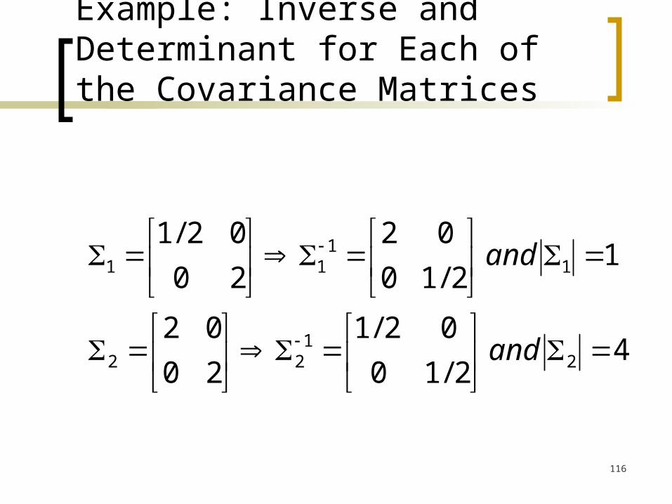
Example: Inverse and Determinant for Each of the Covariance Matrices

42/10

02/1

20

02

12/10

02

20

02/1

21

22

11

11

and

and

117

Example : A Discriminant Function for Class 1

)(ln632

3622

1

)(ln6

33

262

2

1

)(ln1ln2

1

6

3

2/10

0263

2

1)(

)(ln||ln2

1)()(

2

1)(

Since

122

11

12

121

12

1211

1

Pxx

xx

Px

xxx

Px

xxxxg

Pxxxg iiiit

ii

118

Example

)(ln1834

6

)(ln3662

1222

1

)(ln632

3622

1)(

12

22

121

12

22

121

122

111

Pxx

xx

Pxx

xx

Pxx

xxxg

119

Example : A Discriminant Function for Class 2

)(ln2ln234

1

)(ln2ln2

3)2()3(

4

1

)(ln4ln2

1

2

3

2/10

02/123

2

1)(

)(ln||ln2

1)()(

2

1)(

Also,

22

22

1

22

121

22

1212

1

Pxx

Px

xxx

Px

xxxxg

Pxxxg iiiit

ii

120

Example

)(ln2ln4

13

42

3

4

)(ln2ln13464

1

)(ln2ln234

1)(

Hence,

22

22

1

21

22221

21

22

22

12

Pxx

xx

Pxxxx

Pxxxg

121

Example : The Class Boundary

2ln184

13

2

9

4

34

2ln4

13

42

3

4183

46

)(ln2ln4

13

42

3

4)(

)(ln1834

6)(

, setting and Assuming

1

21

2

2

22

1

21

2

22

121

22

22

1

21

2

12

22

1211

2121

xx

x

xx

xx

xx

xx

Pxx

xx

xg

Pxx

xxxg

(x)g(x)g)P(ω)P(ω

122

Example : A Quadratic Separator

)quadratic! (a ,514.3125.11875.0

4

2ln18

16

13

8

9

16

3

2ln184

13

2

9

4

34

1212

1

21

2

1

21

2

xxx

xx

x

xx

x

123

Example : Plot of the Discriminant

-6

-4

-2

0

2

4

6

8

10

0 2 4 6 8

x1

x2

Class 1

Class 2

m1

m2

Discriminant

124

Summary Steps for Building a Bayesian Classifier

Collect class exemplars Estimate class a priori probabilities Estimate class means Form covariance matrices, find the

inverse and determinant for each Form the discriminant function for each

class

125

Using the Classifier

Obtain a measurement vector x Evaluate the discriminant function gi(x)

for each class i = 1,…,c Decide x is in the class j if gj(x) > gi(x)

for all i j

126


Criterions

127


Minimun error rate Criterion

128

Minimum-Error-Rate Classification If action is taken and the true state is ,

then the decision is correct if and in error if

Error rate (the probability of error) is to be minimized

Symmetrical or zero-one loss function

Conditional risk

cjiji

jiji ,,1,,

,1

,0)|(

)|(1)|()|()|(1

xxx ijj

c

jii PPR

ij

ji ji

129


130


Minimax Criterion

131

Bayesian Decision Rule:Two-Category Classification

)(

)(

)(

)(

)|(

)|(

1

2

1121

2212

2

1

P

P

p

p

x

xDecide 1 if

LikelihoodRatio

Threshold

Minimax criterion deals with the case thatthe prior probabilities are unknown.

132

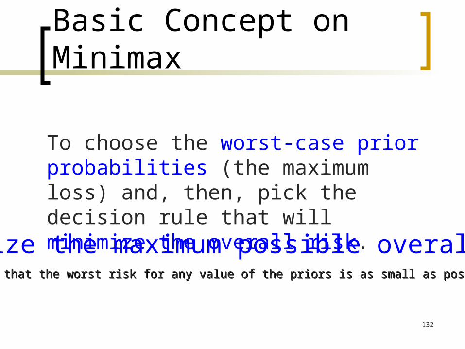
Basic Concept on Minimax

To choose the worst-case prior probabilities (the maximum loss) and, then, pick the decision rule that will minimize the overall risk.

Minimize the maximum possible overall risk.So that the worst risk for any value of the priors is as small as possibleSo that the worst risk for any value of the priors is as small as possible

133

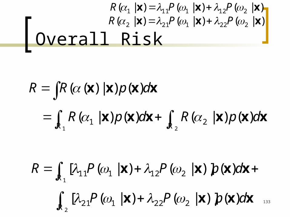
Overall Risk

xxxx dpRR )()|)((

21

)()|()()|( 21 RRxxxxxx dpRdpR

)|()|()|( 2121111 xxx PPR )|()|()|( 2221212 xxx PPR

2

1

)()]|()|([

)()]|()|([

222121

212111

R

R

xxxx

xxxx

dpPP

dpPPR

134

Overall Risk

2

1

)()]|()|([

)()]|()|([

222121

212111

R

R

xxxx

xxxx

dpPP

dpPPR

)(

)()|()|(

x

xx

p

PpP ii

i

)(

)()|()|(

x

xx

p

PpP ii

i

2

1

)]|()()|()([

)]|()()|()([

22221121

22121111

R

R

xxx

xxx

dpPpP

dpPpPR

135

Overall Risk )(1)( 12 PP )(1)( 12 PP

2

1

)]|()()|()([

)]|()()|()([

22221121

22121111

R

R

xxx

xxx

dpPpP

dpPpPR

2

1

)}|()](1[)|()({

)}|()](1[)|()({

21221121

21121111

R

R

xxx

xxx

dpPpP

dpPpPR

1 2

1 1

2 2

12 2 22 2

11 1 1 12 1 2

21 1 1 22 1 2

( | ) ( | )

( ) ( | ) ( ) ( | )

( ) ( | ) ( ) ( | )

R p d p d

P p d P p d

P p d P p d

x x x x

x x x x

x x x x

R R

R R

R R

136

Overall Risk

1 2

1 1

2 2

12 2 22 2

11 1 1 12 1 2

21 1 1 22 1 2

( | ) ( | )

( ) ( | ) ( ) ( | )

( ) ( | ) ( ) ( | )

R p d p d

P p d P p d

P p d P p d

x x x x

x x x x

x x x x

R R

R R

R R

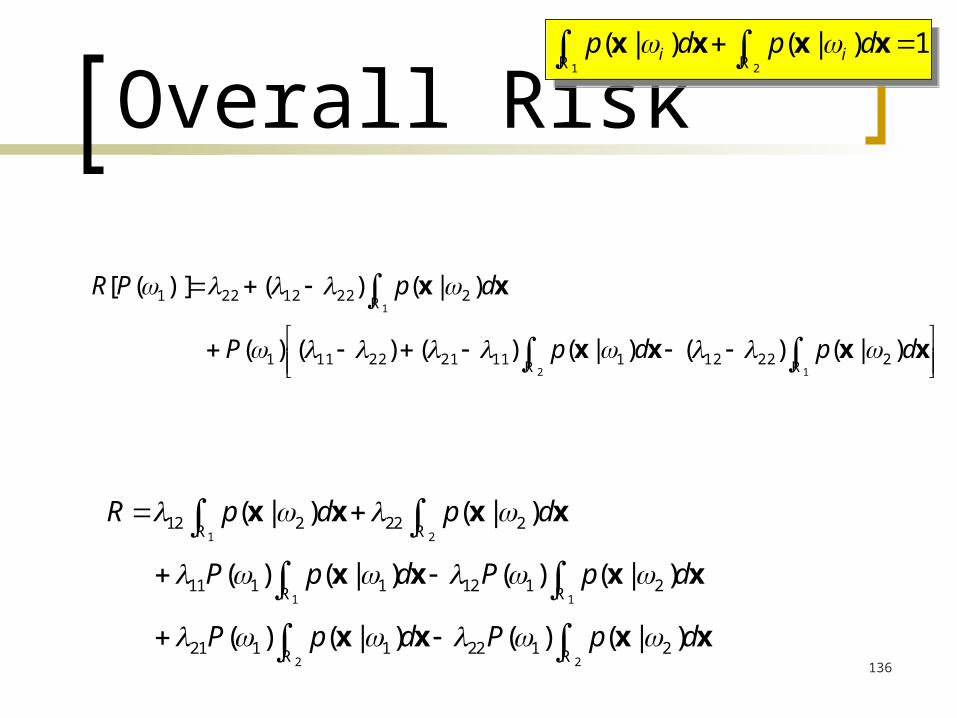
1)|()|(21

RRxxxx dpdp ii 1)|()|(

21

RRxxxx dpdp ii

12

1

)|()()|()()()(

)|()()]([

222121112122111

22212221

RR

R

xxxx

xx

dpdpP

dpPR

137

Overall Risk

12

1

)|()()|()()()(

)|()()]([

222121112122111

22212221

RR

R

xxxx

xx

dpdpP

dpPR

The overall risk for a particular P(1).

The value depends onthe setting of decision boundary

The value depends onthe setting of decision boundary

R(x) = ax + bR(x) = ax + b

138

Overall Risk

12

1

)|()()|()()()(

)|()()]([

222121112122111

22212221

RR

R

xxxx

xx

dpdpP

dpPR

= 0 for minimax solution

= R mm, minimax risk

R(x) = ax + bR(x) = ax + b

Independent on the value of P(i).

139

Minimax Risk

12

1

)|()()|()()()(

)|()()]([

222121112122111

22212221

RR

R

xxxx

xx

dpdpP

dpPR

1

)|()( 2221222 Rxx dpRmm

2

)|()( 1112111 Rxx dp

140

Error Probability

12

1

)|()()|()()()(

)|()()]([

222121112122111

22212221

RR

R

xxxx

xx

dpdpP

dpPR

Use 0/1 loss function

12

1

)|()|()(

)|()]([

211

21

RR

R

xxxx

xx

dpdpP

dpPPerror

141

Minimax Error-Probability

1

)|()( 2Rxx dperrorPmm

2

)|( 1Rxx dp

Use 0/1 loss function

P( 1| 2) P( 2| 1)

12

1

)|()|()(

)|()]([

211

21

RR

R

xxxx

xx

dpdpP

dpPPerror

142


R1 R2

1 2

1

)|()( 2Rxx dperrorPmm

2

)|( 1Rxx dp

P( 1| 2) P( 2| 1)

12

1

)|()|()(

)|()]([

211

21

RR

R

xxxx

xx

dpdpP

dpPPerror

12

1

)|()|()(

)|()]([

211

21

RR

R

xxxx

xx

dpdpP

dpPPerror

143


12

1

)|()|()(

)|()]([

211

21

RR

R

xxxx

xx

dpdpP

dpPPerror

12

1

)|()|()(

)|()]([

211

21

RR

R

xxxx

xx

dpdpP

dpPPerror

144


Neyman-Pearson Criterion

145

Bayesian Decision Rule:Two-Category Classification

)(

)(

)(

)(

)|(

)|(

1

2

1121

2212

2

1

P

P

p

p

x

xDecide 1 if

LikelihoodRatio

Threshold

Neyman-Pearson Criterion deals with the case that both loss functions and the prior probabilities are unknown.

146

Signal Detection Theory The theory of signal detection theory evolved

from the development of communications and radar equipment the first half of the last century.

It migrated to psychology, initially as part of sensation and perception, in the 50's and 60's as an attempt to understand some of the features of human behavior when detecting very faint stimuli that were not being explained by traditional theories of thresholds.

147

The situation of interest A person is faced with a stimulus (signal) that is

very faint or confusing.

The person must make a decision, is the signal there or not.

What makes this situation confusing and difficult is the presences of other mess that is similar to the signal. Let us call this mess noise.

148

Example

Noise is present both in the environment and in the sensory system of the observer.

The observer reacts to the momentary total activation of the sensory system, which fluctuates from moment to moment, as well as responding to environmental stimuli, which may include a signal.

149

Signal Detection Theory

Can we measure the discriminability of the problem?Can we do this independent of the threshold x*?

Suppose we want to detect a single pulse from a signal.

We assume the signal has some random noise.

When the signal is present we observe a normal distribution with mean u2.When the signal is not present we observe a normal distribution with mean u1.We assume same standard deviation.

Discriminability:

d’ = | u2 – u1 | / σ

150

Example A radiologist is examining a CT scan, looking for

evidence of a tumor. A Hard job, because there is always some

uncertainty.

There are four possible outcomes: hit (tumor present and doctor says "yes'') miss (tumor present and doctor says "no'') false alarm (tumor absent and doctor says "yes") correct rejection (tumor absent and doctor says "no").

Two types of Error

151

Correct RejectionCorrect Rejection

The Four Cases

P(1|1)

MissMiss

False AlarmsFalse Alarms HitHit

Signal (tumor)

Absent (1) Present (2)

Decision

No (1)

Yes (2)P(2|2)

P(1|2)

P(2|1)

Signal detection theory was developed to help us understand how a continuous and ambiguous signal can lead to a binary yes/no decision.

Signal detection theory was developed to help us understand how a continuous and ambiguous signal can lead to a binary yes/no decision.

152No (1) Yes (2)

Decision Making

d’Noise

1

Noise + Signal

2

Criterion

Hit

FalseAlarm

Discriminability

||' 12 d

||' 12 d

Based on expectancy)decision bias(

P(2|2)

P(2|1)

153

154

Signal Detection Theory

How do we find d’ if we do not know u1, u2, or x*?

From the data we can compute:

1. P( x > x* | w2) a hit.

2. P( x > x* | w1) a false alarm.

3. P( x < x* | w2) a miss.

4. P( x < x* | w1) a correct rejection.

If we plot a point in a space representing hit and false alarm rates,then we have a ROC (receiver operating characteristic) curve.

With it we can distinguish between discriminability and bias.

155

ROC Curve(Receiver Operating Characteristic)

Hit

FalseAlarm

PH=P(2|2)

PFA=P(2|1)

156

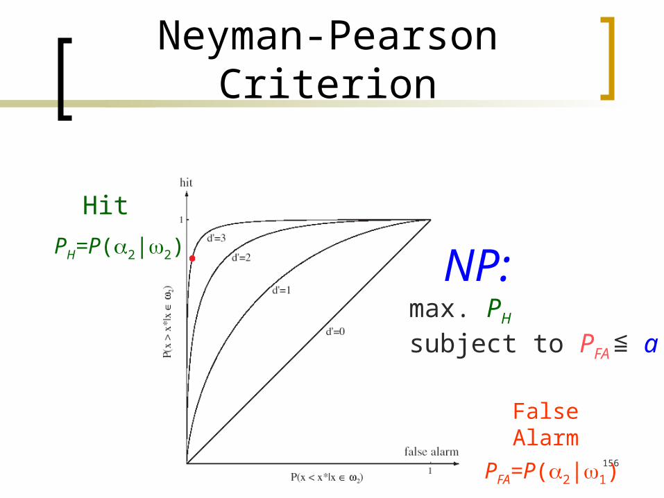
Neyman-Pearson Criterion

FalseAlarm

PFA=P(2|1)

NP:max. PH

subject to PFA ≦ a

Hit

PH=P(2|2)

Documents

1 Bayesian Decision Theory Z. Ghassabi. 2 Outline What is pattern recognition? What is classification? Need for Probabilistic Reasoning Probabilistic