1

2

3

4

5

6

7

8

9

10

11

12

13

14

15

16

17

18

19

20

21

22

23

24

25

26

27

28

29

30

31

32

33

34

35

36

37

38

39

40

41

42

43

44

45

46

47

48

49

What do we need from a probabilistic programminglanguage to support Bayesian workflow?

BOB CARPENTER, Flatiron Institute, New York City

This talk is a survey of the model building and inference steps required for a probabilistic programminglanguage to support a pragmatic Bayesian workflow. Pragmatic Bayesians eschew both of the opposinghistorical traditions of subjective Bayes (encode exactly your subjective beliefs as priors and turn the crank) orobjective Bayes (devise “uninformative” priors and turn the crank). Instead, we follow amore agile methodologywhich combines exploratory data analysis with exploratorymodel fitting, analysis, and visualization, to producecalibrated and sharp inferences for unknown quantities of interest.

1 INTRODUCTIONDeveloping, coding, and applying Bayesian models is much like developing software. We need anagile development process with lots of feedback and fail-fast mechanisms Gelman et al. [2020].1In this paper, I’m going to zoom in on the inference steps required to support workflow and theimplications for developing probabilistic programming languages.The most widely used probabilistic programming languages for applied statistics, Stan and

PyMC3, are not flexible enough to support workflow without rewriting models [Carpenter et al.2017; Salvatier et al. 2016]. BUGS, one of the very first, if not the first, probabilistic programminglanguage, provides just the right level of language flexibility to support workflow, but is lacking inlanguage expressiveness and in support for efficient inference [Gilks et al. 1994; Lunn et al. 2012].

2 THE NITTY GRITTY OF BAYESIANWORKFLOWGelman et al. [2013, Section 1.1] summarizes Bayesian data analysis as being about “practicalmethods for making inferences from data using probability models for quantities we observe andfor quantities about which we wish to learn.” It outlines the process as (1) set up a joint probabilitymodel with density p(θ ,y) for all observable (y) and unobservable (θ ) quantities, (2) condition onobserved data to generate a posterior distribution with density p(θ | y), and (3) evaluate the fit ofthe model and the implications of the resulting posterior.Gelman et al. [2020, Section 1.2] motivate expanding our scope beyond the inference step (2

above), because (a) computation can be challenging and fail, (b) we don’t know what model weneed to fit or even can fit with given data and that model will change as we gather more data, (c)we need to understand the fit of a model to data, and it helps to put this in perspective of morethan one model, and (d) presenting multiple models that reach different substantive conclusionshelps illustrate issues of model choice.

3 INFERENCE REQUIRED FOR BAYESIANWORKFLOWBayesian workflow as envisioned by Gelman et al. [2020], involves multiple steps, as shown inFigure 1. This section explains these steps and the inference required for them from a probabilisticprogramming language.

3.1 Prior predictive checksPrior predictive checks are used to evaluate model behavior before data is observed (i.e., where theposterior is equivalent to the prior) [Box 1980]. Given a joint density p(θ ,y), prior predictive checks1This work is being extended to an open-access book, https://github.com/jgabry/bayes-workflow-book

Author’s address: Bob Carpenter, Flatiron Institute, New York City, bcarpenter@flatironinstitute.org.

50

51

52

53

54

55

56

57

58

59

60

61

62

63

64

65

66

67

68

69

70

71

72

73

74

75

76

77

78

79

80

81

82

83

84

85

86

87

88

89

90

91

92

93

94

95

96

97

98

2 Carpenter, B.

Figure 1: Overview of the steps we currently consider in Bayesian workflow. Numbers in bracketsrefer to sections of this paper where the steps are discussed. The chart aims to show possiblesteps and paths an individual analysis may go through, with the understanding that any particularanalysis will most likely not involve all of these steps. One of our goals in studying workflow is tounderstand how these ideas fit together so they can be applied more systematically.

5

Fig. 1. Overview of steps in Bayesian workflow. Each of the grey boxes involves forms of model fitting that benefitfrom probabilistic programming languages. Figure reproduced from Gelman et al. [2020, p. 5].

require sampling from themarginal data distribution,ysim ∼ p(y), wherep(y) =∫RN

p(y | θ )·p(θ ) dθmarginalizes out the parameters θ by averaging the sampling distribution p(y | θ ) over the priorp(θ ). Prior predictive checks evaluate whether the data generated from the prior is realistic bycomparing it to actual data; see Gabry et al. [2019] for examples. The comparison is based onsimulating multiple data sets ysim(1), . . .ysim(M ), computing a statistic t(ysim(m)) for each simulation,and comparing the quantile of the same statistic t(y) of the actual data. Any statistics of the data maybe used, including central tendencies like mean and median, variance, skew, quantiles (includingminimum or maximum values), etc. Unlike for posterior predictive checks (see below), we do notexpect calibration at this stage.

3.2 Simulation-based calibrationIt is common to generate fake data, either by choosing reasonable parameter values by hand orgenerating them from the prior. For example, to generate a fake data set ysim ∼ p(y) from the priorpredictive distribution, it suffices to draw θ sim ∼ p(θ ) from the prior and ysim ∼ p(y | θ sim) fromthe sampling distribution to produce a joint draw ysim, θ sim ∼ p(y, θ ). Then we apply inference andtake a sample of draws θ (m) ∼ p(θ | ysim) from the posterior and then measure if the posterior for θis consistent with the simulated value θ sim.To make this procedure more precise and automatic, we can use simulation-based calibration

(SBC), which as its name implies, evaluates whether posteriors are properly calibrated [Cook et al.2006; Talts et al. 2018]. Suppose we’ve drawn simulated data and parameters ysim, θ sim ∼ p(y, θ ).Now if we take a posterior draw θ (m) ∼ p(θ | ysim), the chain rule tells us that ysim, θ (m) ∼ p(y, θ )is also a draw from the joint distribution. If we take multiple posterior draws, the rank of of θ simamong the θ (1), . . . , θ (M ) should be uniformly distributed over multiple simulations θ sim. The resultis a calibration test for posteriors given well-specified data drawn from the prior. SBC requiresproper priors which are restrictive enough that draws from them do not cause numerical issues like

99

100

101

102

103

104

105

106

107

108

109

110

111

112

113

114

115

116

117

118

119

120

121

122

123

124

125

126

127

128

129

130

131

132

133

134

135

136

137

138

139

140

141

142

143

144

145

146

147

What do we need from a probabilistic programming language to support Bayesian workflow? 3

underflow or overflow; for example, if our predictors are unit scale and we draw logistic regressioncoefficients from a prior βk ∼ normal(0, 100) or even worse βk ∼ cauchy(0, 1), then we will almostcertainly get draws that cause numerical overflow or underflow in evaluating the link function.

3.3 Posterior predictive checksPosterior predictive checks (PPC) provide a Bayesian approach to goodness-of-fit evaluations[Gelman et al. 1996; Guttman 1967; Rubin 1984]. They are like prior predictive checks, but wecheck discrepancies in statistics between our observed data and posterior simulations conditionedon our observed data. Technically, we start with multiple draws θ sim(1), . . . , θ sim(M ) ∼ p(θ | yobs)from the posterior. For each of these draws, we simulate data from the sampling distribution,ysim(m) ∼ p(y | θ sim(m)). Together, this amounts to drawing from the posterior predictive distributionysim(m) ∼ p(y | yobs).

From a machine learning perspective, this is a kind of “cheating” in which we evaluate the fit tothe “training” data, not to held out data. But don’t worry, this isn’t our final test. We just use thisrelatively cheap step to try to reject models before going on to check their held-out behavior (seethe next section), because if they can’t represent the data they’re fit with, they’re unlikely to fitheld out data.

3.4 Cross-validationCross-validation evaluates how well a model is able to predict a subset of the data when fit to thecomplementary subset of data [Stone 1974]. In the limit, leave-one-out cross-validation evaluateshow well a model predicts a single data item when fit with all of the other data items [Vehtari et al.2017]. Cross-validation relies on being able to subdivide the data into two pieces yobs = yobs1 ,y

obs2 ,

and evaluate (not sample from) the posterior predictive distribution, p(yobs1 | yobs2 ). We can evaluatethe posterior predictive distribution at a point using MCMC draws θ (m) ∼ p(θ | yobs) with2

p(yobs1 | yobs2 ) = E[p(yobs1 | θ ) | yobs2 ] =∫p(yobs1 | θ ) · p(θ | yobs2 ) dθ ≈ 1

M∑Mm=1 p(y

obs1 | θ (m)).

3.5 Sensitivity analysisThe certainty through which a parameter is known can be measured through the Bayesian pos-terior. But this is a model-based decision and there is further uncertainty due to choice of modelcomponents (likelihood and prior) and choice of constants like hyperparameters within a givenmodel structure. Checking how much these decisions matter is a matter of sensitivity analysis(Oakley and O’Hagan [2004] provide a broad survey).

For example, suppose we have regression coefficients with a prior βk ∼ normal(0,σ ) and we’vechosen to set σ = 2. We can carry out inference for σ = 1 or σ = 4 and see how the results change.Or we could replace the normal distribution with a Student-t distribution of the same variance andsee what happens.The traditional approach in applied mathematics is to compute a derivative (or second-order

derivative) of the quantity of interest [Saltelli et al. 2004],

∂∂σ E[f (α) | y,σ , . . .]

����σ=2.

We can evaluate sensitivity to data elements in the same way. Or we can evaluate fits with andwithout data items to measure their effect in the context of other data items. All of this can becarried out in a Bayesian framework using automatic differentiation, as shown by Giordano [2019].2For numerical stability, this calculation needs to be carried out on the log scale where logp(yobs

1 | yobs2 ) ≈ − logM +

log_sum_expMm=1 logp(yobs1 | θ (m)), for draws θ (m) ∼ p(y | yobs

2 ).

148

149

150

151

152

153

154

155

156

157

158

159

160

161

162

163

164

165

166

167

168

169

170

171

172

173

174

175

176

177

178

179

180

181

182

183

184

185

186

187

188

189

190

191

192

193

194

195

196

4 Carpenter, B.

3.6 Model comparison by calibration and sharpnessAssuming we have two models that pass all of our diagnostics, how do we compare them? Thestandard pragmatic Bayesian approach is to compare them in terms of calibration and sharpness[Gneiting et al. 2007]. Simulation-based calibration made sure inference for parameters was self-consistently calibrated. Now we want to make sure that inference for held out data is calibrated.Calibration is the analogue of unbiased estimation for Bayesian posteriors—we want our probabilitystatements about future data to have the appropriate frequentist coverage [Dawid 1982]. Sharpnessis the analogue of low-bias estimation; sharp estimates have low variance, or similarly, low entropy.For example, suppose I’m trying to compare 99% intervals for Republican vote share in the nextpresidential election. An interval of (0.489, 0.491) is sharper than (0.46, 0.50).

We can evaluate calibration and sharpness using so-called “proper scoring metrics”, such as rootmean squared error of estimations or in a probabilistic way using held-out log density [Dawid 2007;Gneiting and Raftery 2007]. Such evaluations are based on evaluating (not sampling) posteriorpredictive inferences p(ynew | yobs) for new data given observed data.

We do not recommend using Bayes factors, because they are ratios of prior predictive densitiesrather than posterior predictive densities. For example, if we have two data models p(y | M1) andp(y | M2), then Bayes factors compare the ratio of p(yobs | M1) to p(yobs | M2) for some observeddata yobs. This averages the predictions for yobs over the prior p(θ ), with

p(yobs | M) = E[p(yobs | θ )] =∫p(yobs | θ ) · p(θ ) dθ .

Wewould rather focus on posterior predictive inference and evaluation on held out dataynew, whichinstead compares the posterior predictive densities of p(ynew | yobs,M1) and p(ynew | yobs,M2).These average predictions over the posterior p(θ | yobs (for a modelM1,M2, etc.), with

p(ynew | yobs) = E[p(ynew | θ ) | yobs] =∫p(ynew | θ ) · p(θ | yobs) dθ .

3.7 Summary of inference and modeling required for workflowTo fully support inference proposed for workflow, we need to be able to sample from the followingmarginal, joint and conditional distributions for any model p(θ ,y) of interest.

• ysim ∼ p(y) [prior predictive checks]• ysim, θ sim ∼ p(y, θ ) [simulation-based calibration]• θ (m) ∼ p(θ | ysim) [simulation-based calibration]• ysim ∼ p(y | yobs) [posterior predictive checks]

We also need to be able to evaluate the following quantity.• p(yobs1 | yobs2 ) = E[p(yobs1 | θ ) | yobs2 ] [cross-validation]

To evaluate Bayes factors, we’d also need to be able to evaluate• p(yobs) = E[p(yobs | θ )] =

∫p(yobs | θ ) · p(θ ) dθ .

Furthermore, all of the ways in which we might modify a model need to be accommodated somehow.I dream of a workbench that keeps track of the choices I make as a I go so that they can be easily nav-igated and later included in a final presentation. As is, I wind up with file names like irt-2pl.stan,irt-2pl-hier.stan, irt-2pl-std-norm-student-zero-centered-hier-difficulty.stan, andso on until it’s impossible to keep track of which model is doing what.

4 REMEDIATING PROBLEMS DURINGWORKFLOWWhen computational or statistical problems arise from models, there are various steps we mighttake to mitigate them. These are outlined in the “modify the model” box of the workflow diagramin Figure 1. At the most radical, we might just throw out a model and start again. But typically we

197

198

199

200

201

202

203

204

205

206

207

208

209

210

211

212

213

214

215

216

217

218

219

220

221

222

223

224

225

226

227

228

229

230

231

232

233

234

235

236

237

238

239

240

241

242

243

244

245

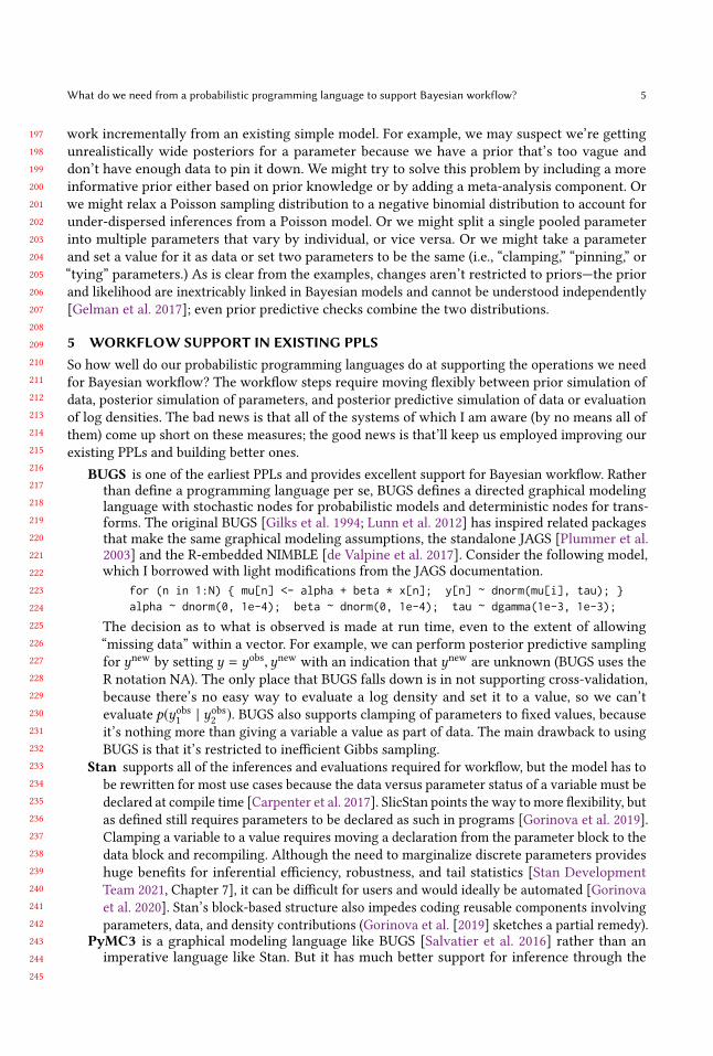
What do we need from a probabilistic programming language to support Bayesian workflow? 5

work incrementally from an existing simple model. For example, we may suspect we’re gettingunrealistically wide posteriors for a parameter because we have a prior that’s too vague anddon’t have enough data to pin it down. We might try to solve this problem by including a moreinformative prior either based on prior knowledge or by adding a meta-analysis component. Orwe might relax a Poisson sampling distribution to a negative binomial distribution to account forunder-dispersed inferences from a Poisson model. Or we might split a single pooled parameterinto multiple parameters that vary by individual, or vice versa. Or we might take a parameterand set a value for it as data or set two parameters to be the same (i.e., “clamping,” “pinning,” or“tying” parameters.) As is clear from the examples, changes aren’t restricted to priors—the priorand likelihood are inextricably linked in Bayesian models and cannot be understood independently[Gelman et al. 2017]; even prior predictive checks combine the two distributions.

5 WORKFLOW SUPPORT IN EXISTING PPLSSo how well do our probabilistic programming languages do at supporting the operations we needfor Bayesian workflow? The workflow steps require moving flexibly between prior simulation ofdata, posterior simulation of parameters, and posterior predictive simulation of data or evaluationof log densities. The bad news is that all of the systems of which I am aware (by no means all ofthem) come up short on these measures; the good news is that’ll keep us employed improving ourexisting PPLs and building better ones.

BUGS is one of the earliest PPLs and provides excellent support for Bayesian workflow. Ratherthan define a programming language per se, BUGS defines a directed graphical modelinglanguage with stochastic nodes for probabilistic models and deterministic nodes for trans-forms. The original BUGS [Gilks et al. 1994; Lunn et al. 2012] has inspired related packagesthat make the same graphical modeling assumptions, the standalone JAGS [Plummer et al.2003] and the R-embedded NIMBLE [de Valpine et al. 2017]. Consider the following model,which I borrowed with light modifications from the JAGS documentation.

for (n in 1:N) { mu[n] <- alpha + beta * x[n]; y[n] ~ dnorm(mu[i], tau); }alpha ~ dnorm(0, 1e-4); beta ~ dnorm(0, 1e-4); tau ~ dgamma(1e-3, 1e-3);

The decision as to what is observed is made at run time, even to the extent of allowing“missing data” within a vector. For example, we can perform posterior predictive samplingfor ynew by setting y = yobs,ynew with an indication that ynew are unknown (BUGS uses theR notation NA). The only place that BUGS falls down is in not supporting cross-validation,because there’s no easy way to evaluate a log density and set it to a value, so we can’tevaluate p(yobs1 | yobs2 ). BUGS also supports clamping of parameters to fixed values, becauseit’s nothing more than giving a variable a value as part of data. The main drawback to usingBUGS is that it’s restricted to inefficient Gibbs sampling.

Stan supports all of the inferences and evaluations required for workflow, but the model has tobe rewritten for most use cases because the data versus parameter status of a variable must bedeclared at compile time [Carpenter et al. 2017]. SlicStan points the way to more flexibility, butas defined still requires parameters to be declared as such in programs [Gorinova et al. 2019].Clamping a variable to a value requires moving a declaration from the parameter block to thedata block and recompiling. Although the need to marginalize discrete parameters provideshuge benefits for inferential efficiency, robustness, and tail statistics [Stan DevelopmentTeam 2021, Chapter 7], it can be difficult for users and would ideally be automated [Gorinovaet al. 2020]. Stan’s block-based structure also impedes coding reusable components involvingparameters, data, and density contributions (Gorinova et al. [2019] sketches a partial remedy).

PyMC3 is a graphical modeling language like BUGS [Salvatier et al. 2016] rather than animperative language like Stan. But it has much better support for inference through the

246

247

248

249

250

251

252

253

254

255

256

257

258

259

260

261

262

263

264

265

266

267

268

269

270

271

272

273

274

275

276

277

278

279

280

281

282

283

284

285

286

287

288

289

290

291

292

293

294

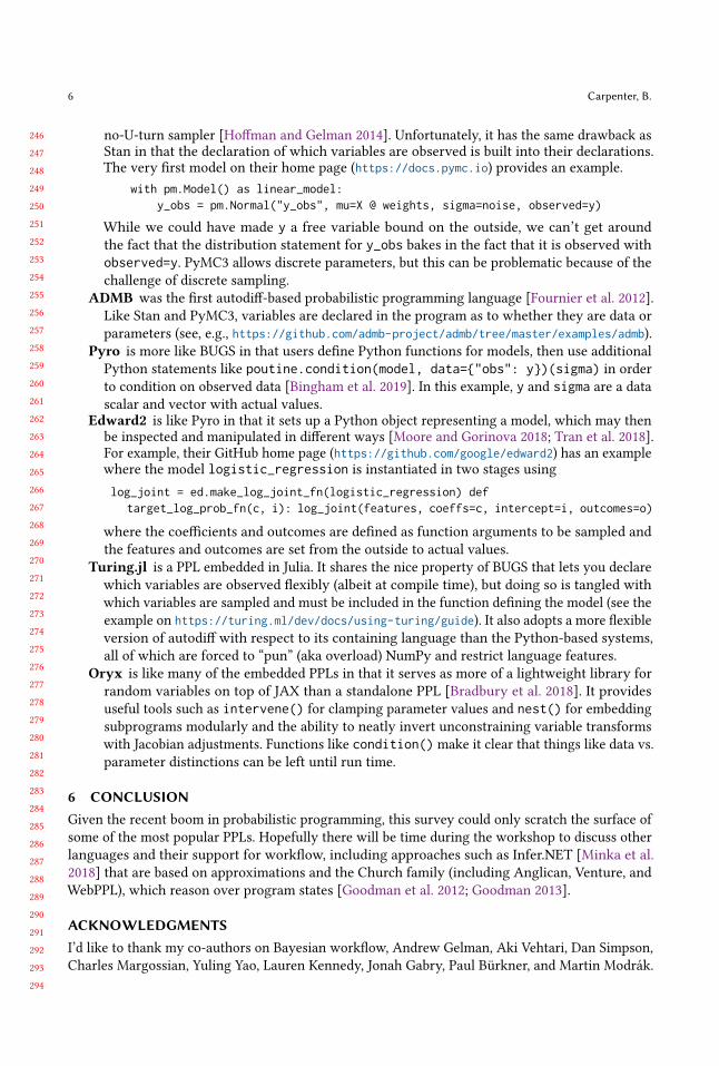
6 Carpenter, B.

no-U-turn sampler [Hoffman and Gelman 2014]. Unfortunately, it has the same drawback asStan in that the declaration of which variables are observed is built into their declarations.The very first model on their home page (https://docs.pymc.io) provides an example.

with pm.Model() as linear_model:y_obs = pm.Normal("y_obs", mu=X @ weights, sigma=noise, observed=y)

While we could have made y a free variable bound on the outside, we can’t get aroundthe fact that the distribution statement for y_obs bakes in the fact that it is observed withobserved=y. PyMC3 allows discrete parameters, but this can be problematic because of thechallenge of discrete sampling.

ADMB was the first autodiff-based probabilistic programming language [Fournier et al. 2012].Like Stan and PyMC3, variables are declared in the program as to whether they are data orparameters (see, e.g., https://github.com/admb-project/admb/tree/master/examples/admb).

Pyro is more like BUGS in that users define Python functions for models, then use additionalPython statements like poutine.condition(model, data={"obs": y})(sigma) in orderto condition on observed data [Bingham et al. 2019]. In this example, y and sigma are a datascalar and vector with actual values.

Edward2 is like Pyro in that it sets up a Python object representing a model, which may thenbe inspected and manipulated in different ways [Moore and Gorinova 2018; Tran et al. 2018].For example, their GitHub home page (https://github.com/google/edward2) has an examplewhere the model logistic_regression is instantiated in two stages usinglog_joint = ed.make_log_joint_fn(logistic_regression) def

target_log_prob_fn(c, i): log_joint(features, coeffs=c, intercept=i, outcomes=o)

where the coefficients and outcomes are defined as function arguments to be sampled andthe features and outcomes are set from the outside to actual values.

Turing.jl is a PPL embedded in Julia. It shares the nice property of BUGS that lets you declarewhich variables are observed flexibly (albeit at compile time), but doing so is tangled withwhich variables are sampled and must be included in the function defining the model (see theexample on https://turing.ml/dev/docs/using-turing/guide). It also adopts a more flexibleversion of autodiff with respect to its containing language than the Python-based systems,all of which are forced to “pun” (aka overload) NumPy and restrict language features.

Oryx is like many of the embedded PPLs in that it serves as more of a lightweight library forrandom variables on top of JAX than a standalone PPL [Bradbury et al. 2018]. It providesuseful tools such as intervene() for clamping parameter values and nest() for embeddingsubprograms modularly and the ability to neatly invert unconstraining variable transformswith Jacobian adjustments. Functions like condition() make it clear that things like data vs.parameter distinctions can be left until run time.

6 CONCLUSIONGiven the recent boom in probabilistic programming, this survey could only scratch the surface ofsome of the most popular PPLs. Hopefully there will be time during the workshop to discuss otherlanguages and their support for workflow, including approaches such as Infer.NET [Minka et al.2018] that are based on approximations and the Church family (including Anglican, Venture, andWebPPL), which reason over program states [Goodman et al. 2012; Goodman 2013].

ACKNOWLEDGMENTSI’d like to thank my co-authors on Bayesian workflow, Andrew Gelman, Aki Vehtari, Dan Simpson,Charles Margossian, Yuling Yao, Lauren Kennedy, Jonah Gabry, Paul Bürkner, and Martin Modrák.

295

296

297

298

299

300

301

302

303

304

305

306

307

308

309

310

311

312

313

314

315

316

317

318

319

320

321

322

323

324

325

326

327

328

329

330

331

332

333

334

335

336

337

338

339

340

341

342

343

What do we need from a probabilistic programming language to support Bayesian workflow? 7

REFERENCESEli Bingham, Jonathan P Chen, Martin Jankowiak, Fritz Obermeyer, Neeraj Pradhan, Theofanis Karaletsos, Rohit Singh,

Paul Szerlip, Paul Horsfall, and Noah D Goodman. 2019. Pyro: Deep universal probabilistic programming. The Journal ofMachine Learning Research 20, 1 (2019), 973–978.

George EP Box. 1980. Sampling and Bayes’ inference in scientific modelling and robustness. Journal of the Royal StatisticalSociety: Series A (General) 143, 4 (1980), 383–404.

James Bradbury, Roy Frostig, Peter Hawkins, Matthew James Johnson, Chris Leary, Dougal Maclaurin, George Necula,Adam Paszke, Jake VanderPlas, Skye Wanderman-Milne, and Qiao Zhang. 2018. JAX: composable transformations ofPython+NumPy programs. http://github.com/google/jax

Bob Carpenter, Andrew Gelman, Matthew D Hoffman, Daniel Lee, Ben Goodrich, Michael Betancourt, Marcus A Brubaker,Jiqiang Guo, Peter Li, and Allen Riddell. 2017. Stan: a probabilistic programming language. Journal of Statistical Software76, 1 (2017), 1–32.

Samantha R Cook, Andrew Gelman, and Donald B Rubin. 2006. Validation of software for Bayesian models using posteriorquantiles. Journal of Computational and Graphical Statistics 15, 3 (2006), 675–692.

A Philip Dawid. 1982. The well-calibrated Bayesian. J. Amer. Statist. Assoc. 77, 379 (1982), 605–610.A Philip Dawid. 2007. The geometry of proper scoring rules. Annals of the Institute of Statistical Mathematics 59, 1 (2007),

77–93.Perry de Valpine, Daniel Turek, Christopher J Paciorek, Clifford Anderson-Bergman, Duncan Temple Lang, and Rastislav

Bodik. 2017. Programming with models: writing statistical algorithms for general model structures with NIMBLE. Journalof Computational and Graphical Statistics 26, 2 (2017), 403–413.

David A Fournier, Hans J Skaug, Johnoel Ancheta, James Ianelli, Arni Magnusson, Mark N Maunder, Anders Nielsen, andJohn Sibert. 2012. AD Model Builder: using automatic differentiation for statistical inference of highly parameterizedcomplex nonlinear models. Optimization Methods and Software 27, 2 (2012), 233–249.

Jonah Gabry, Daniel Simpson, Aki Vehtari, Michael Betancourt, and Andrew Gelman. 2019. Visualization in Bayesianworkflow. Journal of the Royal Statistical Society: Series A (Statistics in Society) 182, 2 (2019), 389–402.

Andrew Gelman, John B Carlin, Hal S Stern, David B Dunson, Aki Vehtari, and Donald B Rubin. 2013. Bayesian DataAnalysis (third ed.). Chapman & Hall/CRC Press.

Andrew Gelman, Xiao-Li Meng, and Hal Stern. 1996. Posterior predictive assessment of model fitness via realized discrepan-cies. Statistica sinica (1996), 733–760.

Andrew Gelman, Daniel Simpson, and Michael Betancourt. 2017. The prior can often only be understood in the context ofthe likelihood. Entropy 19, 10 (2017), 555.

Andrew Gelman, Aki Vehtari, Daniel Simpson, Charles C Margossian, Bob Carpenter, Yuling Yao, Lauren Kennedy, JonahGabry, Paul-Christian Bürkner, and Martin Modrák. 2020. Bayesian workflow. arXiv preprint arXiv:2011.01808 (2020).

Wally R Gilks, Andrew Thomas, and David J Spiegelhalter. 1994. A language and program for complex Bayesian modelling.Journal of the Royal Statistical Society: Series D (The Statistician) 43, 1 (1994), 169–177.

Ryan James Giordano. 2019. On the Local Sensitivity of M-Estimation: Bayesian and Frequentist Applications. Ph.D. Dissertation.UC Berkeley.

Tilmann Gneiting, Fadoua Balabdaoui, and Adrian E Raftery. 2007. Probabilistic forecasts, calibration and sharpness. Journalof the Royal Statistical Society: Series B (Statistical Methodology) 69, 2 (2007), 243–268.

Tilmann Gneiting and Adrian E Raftery. 2007. Strictly proper scoring rules, prediction, and estimation. J. Amer. Statist.Assoc. 102, 477 (2007), 359–378.

Noah Goodman, Vikash Mansinghka, Daniel M Roy, Keith Bonawitz, and Joshua B Tenenbaum. 2012. Church: a languagefor generative models. arXiv preprint arXiv:1206.3255 (2012).

Noah D Goodman. 2013. The principles and practice of probabilistic programming. ACM SIGPLAN Notices 48, 1 (2013),399–402.

Maria Gorinova, Dave Moore, and Matthew Hoffman. 2020. Automatic reparameterisation of probabilistic programs. InInternational Conference on Machine Learning. PMLR, 3648–3657.

Maria I Gorinova, Andrew D Gordon, and Charles Sutton. 2019. Probabilistic programming with densities in SlicStan:efficient, flexible, and deterministic. Proceedings of the ACM on Programming Languages 3, POPL (2019), 1–30.

Irwin Guttman. 1967. The use of the concept of a future observation in goodness-of-fit problems. Journal of the RoyalStatistical Society: Series B (Methodological) 29, 1 (1967), 83–100.

Matthew D Hoffman and Andrew Gelman. 2014. The No-U-Turn sampler: adaptively setting path lengths in HamiltonianMonte Carlo. J. Mach. Learn. Res. 15, 1 (2014), 1593–1623.

David Lunn, Chris Jackson, Nicky Best, Andrew Thomas, and David Spiegelhalter. 2012. The BUGS book: A practicalintroduction to Bayesian analysis. CRC press.

T. Minka, J.M. Winn, J.P. Guiver, Y. Zaykov, D. Fabian, and J. Bronskill. 2018. /Infer.NET 0.3. Microsoft Research Cambridge.http://dotnet.github.io/infer.

344

345

346

347

348

349

350

351

352

353

354

355

356

357

358

359

360

361

362

363

364

365

366

367

368

369

370

371

372

373

374

375

376

377

378

379

380

381

382

383

384

385

386

387

388

389

390

391

392

8 Carpenter, B.

Dave Moore and Maria I Gorinova. 2018. Effect handling for composable program transformations in Edward2. arXivpreprint arXiv:1811.06150 (2018).

Jeremy E Oakley and Anthony O’Hagan. 2004. Probabilistic sensitivity analysis of complex models: a Bayesian approach.Journal of the Royal Statistical Society: Series B (Statistical Methodology) 66, 3 (2004), 751–769.

Martyn Plummer et al. 2003. JAGS: A program for analysis of Bayesian graphical models using Gibbs sampling. In Proceedingsof the 3rd international workshop on distributed statistical computing, Vol. 124. Vienna, Austria., 1–10.

Donald B Rubin. 1984. Bayesianly justifiable and relevant frequency calculations for the applied statistician. The Annals ofStatistics (1984), 1151–1172.

Andrea Saltelli, Stefano Tarantola, Francesca Campolongo, and Marco Ratto. 2004. Sensitivity analysis in practice: a guide toassessing scientific models. Vol. 1. Wiley Online Library.

John Salvatier, Thomas V Wiecki, and Christopher Fonnesbeck. 2016. Probabilistic programming in Python using PyMC3.PeerJ Computer Science 2 (2016), e55.

Stan Development Team. 2021. Stan User’s Guide. https://mc-stan.org/documentationMervyn Stone. 1974. Cross-validatory choice and assessment of statistical predictions. Journal of the Royal Statistical Society:

Series B (Methodological) 36, 2 (1974), 111–133.Sean Talts, Michael Betancourt, Daniel Simpson, Aki Vehtari, and Andrew Gelman. 2018. Validating Bayesian inference

algorithms with simulation-based calibration. arXiv preprint arXiv:1804.06788 (2018).Dustin Tran, Matthew Hoffman, Dave Moore, Christopher Suter, Srinivas Vasudevan, Alexey Radul, Matthew Johnson, and

Rif A Saurous. 2018. Simple, distributed, and accelerated probabilistic programming. arXiv preprint arXiv:1811.02091(2018).

Aki Vehtari, Andrew Gelman, and Jonah Gabry. 2017. Practical Bayesian model evaluation using leave-one-out cross-validation and WAIC. Statistics and Computing 27, 5 (2017), 1413–1432.