Lect. 4. Toward MLA in tensor-product formats B. Khoromskij, Leipzig 2007(L4) 1

Contents of Lecture 4

1. Structured representation of high-order tensors revisited.

- Tucker model.

- Canonical (PARAFAC) model.

- Two-level and mixed models.

2. Multi-linear algebra (MLA) with Kronecker-product data.

- Invariace of some matrix properties.

- Commutator, matrix exponential, eigen-value problem.

- Lyapunov equation.

- Complexity issues.

3. Algebaric methods of tensor-product decomposition.

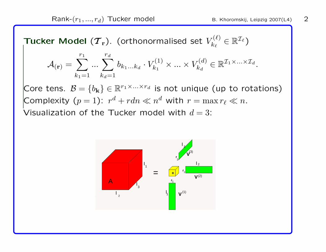
Rank-(r1, ..., rd) Tucker model B. Khoromskij, Leipzig 2007(L4) 2

Tucker Model (T r). (orthonormalised set V(ℓ)kℓ

∈ RIℓ)

A(r) =

r1∑

k1=1

...

rd∑

kd=1

bk1...kd· V

(1)k1

× ... × V(d)kd

∈ RI1×...×Id .

Core tens. B = bk ∈ Rr1×...×rd is not unique (up to rotations)

Complexity (p = 1): rd + rdn ≪ nd with r = max rℓ ≪ n.

Visualization of the Tucker model with d = 3:

=

I 2

I 1

I 3

A B

I 1

r 2

r 1

I 2

I 3

r 3

V

V

V

(1)

(2)

(3)

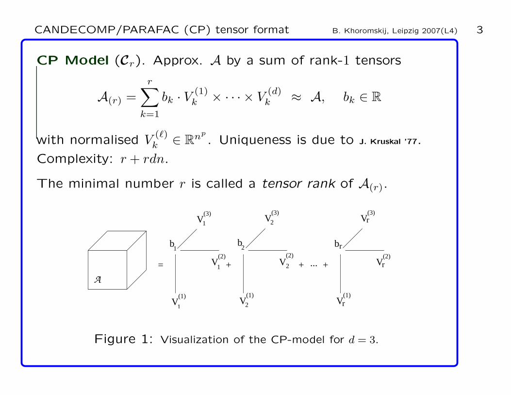
CANDECOMP/PARAFAC (CP) tensor format B. Khoromskij, Leipzig 2007(L4) 3

CP Model (Cr). Approx. A by a sum of rank-1 tensors

A(r) =r∑

k=1

bk · V(1)k × · · · × V

(d)k ≈ A, bk ∈ R

with normalised V(ℓ)k ∈ Rnp

. Uniqueness is due to J. Kruskal ’77.

Complexity: r + rdn.

The minimal number r is called a tensor rank of A(r).

+

b

A

1b

V V V

V V V

V V V

+= ...+

1

1 2

2

2

r

r

r

(1) (1) (1)

(2) (2) (2)

21

(3) (3) (3)

rb

Figure 1: Visualization of the CP-model for d = 3.

Two-level and mixed models B. Khoromskij, Leipzig 2007(L4) 4

Two-level Tucker model T (U ,r,q),

A(r,q) = B ×V(1) × V

(2)... × V(d) ∈ T (U ,r,q) ⊂ C(n,q),

1. B ∈ Rr1×...×rd is retrieved by the rank-q CP model C(r,q)

2. V(ℓ) = [V

(ℓ)1 V

(ℓ)2 ...V

(ℓ)rℓ ] ∈ U, ℓ = 1, ..., d,

U spans fixed (uniform/adaptive) basis;

⇒ O(rd) with r = maxℓ≤d rℓ ⇒ O(dqr) (independent of n !).

Mixed model MC,T :

A = A1 + A2, A1 ∈ Cr1 , A2 ∈ T r2 .

Applies to ”ill-conditioned” tensors.

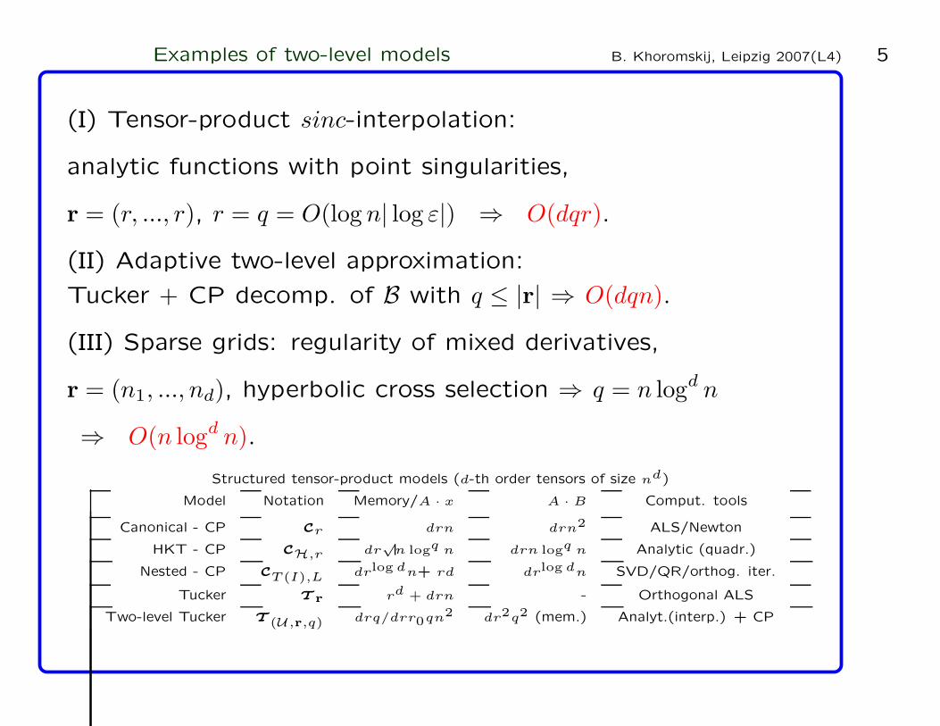
Examples of two-level models B. Khoromskij, Leipzig 2007(L4) 5

(I) Tensor-product sinc-interpolation:

analytic functions with point singularities,

r = (r, ..., r), r = q = O(log n| log ε|) ⇒ O(dqr).

(II) Adaptive two-level approximation:

Tucker + CP decomp. of B with q ≤ |r| ⇒ O(dqn).

(III) Sparse grids: regularity of mixed derivatives,

r = (n1, ..., nd), hyperbolic cross selection ⇒ q = n logd n

⇒ O(n logd n).

Structured tensor-product models (d-th order tensors of size nd)

Model Notation Memory/A · x A · B Comput. tools

Canonical - CP Cr drn drn2 ALS/Newton

HKT - CP CH,r dr√

n logq n drn logq n Analytic (quadr.)

Nested - CP CT (I),L drlog dn+ rd drlog dn SVD/QR/orthog. iter.

Tucker T r rd + drn - Orthogonal ALS

Two-level Tucker T (U,r,q) drq/drr0qn2 dr2q2 (mem.) Analyt.(interp.) + CP

Challenge of multi-factor analysis B. Khoromskij, Leipzig 2007(L4) 6

Paradigm: linear algebra vs. multi-linear algebra.

CP/Tucker tensor-product models have plenty of merits:

1. A(r) is repr. with low cost drn (resp. drn + rd) ≪ nd.

2. V(ℓ)k can be repr. in the data-sparse form:

H-matrix (HKT), wavelet-based (WKT), uniform basis.

3. The core tensor B = bk can be ”sparsified” via CP model.

4. Efficient numerical MLA ⇔ Highly nonlinear problems.

Remark. CP decomposition (unique !) can’t be retrieved by

rotation and truncation of the Tucker model,

Cr = T r if r = 1 ∨ d = 2, but Cr 6⊂ T r if r = |r| ≥ 2 ∧ d ≥ 3.

Little analogy between the cases d ≥ 3 and d = 2 B. Khoromskij, Leipzig 2007(L4) 7

I. rank(A) depends on the number field (say, R or C).

II. We do not know any finite algorithm to compute

r = rank(A), except simple bounds:

rank(A) ≤ nd−1; rank(A) ≤ rank(A1) + ... + rank(And−2)

III. For fixed d and n we do not know the exact value of

maxrank(A). J. Kruskal ’75 proved that:

– for any 2 × 2 × 2 tensor we have maxrank(A) = 3 < 4;

– for 3 × 3 × 3 tensors there holds maxrank(A) = 5 < 9.

IV. “Probabilistic” properties of rank(A): in the set of 2× 2× 2

tensors there is about 79% of rank-2 tensors and 21% of

rank-3 tensors, while rank-1 tensors appear with probability 0.

Clearly, for n × n matrices we have Prank(A) = n = 1.

Little analogy between the cases d ≥ 3 and d = 2 B. Khoromskij, Leipzig 2007(L4) 8

V. However, it is possible to prove very important uniqueness

property within the equivalence classes.

Two CP-type representations are considered as equivalent if either

(a) they differ in the order of terms or

(b) for some set of paramers aℓ

k∈ R such that

dQ

ℓ=1aℓ

k= 1 (k = 1, ..., r),

there is a transform V(ℓ)k

→ aℓ

kV

(ℓ)k

.

A simplified version of the general uniqueness result is the

following (all factors have the same full rank r).

Prop. 1. (J. Kruskal, 1977) Let for each ℓ = 1, ..., d, the vectors

V(ℓ)k , (k = 1, ..., r) with r = rank(A), are linear independent. If

(d − 2)r ≥ d − 1,

then the CP decomposition is uniquely determined up to the

equivalence (a) - (b) above.

Properties of the Kronecker product B. Khoromskij, Leipzig 2007(L4) 9

A tensor A ∈ RI1×...×Id can be viewed as:

A. An element of linear space of vectors with the ℓ2-inner

product and related Frobenius norm, which is a multi-variate

function of the discrete argument A : I1 × ... × Id → R.

B. A mapping A : RI1×...×Iq → R

Iq+1×...×Id (hence, requiring

matrix operations in the tensor format).

Def. 4.1. The Kronecker product (KP) operation A ⊗ B of

two matrices

A = [aij ] ∈ Rm×n, B ∈ R

h×g

is an mh × ng matrix that has the block-representation [aijB].

Ex. 4.1. In general A ⊗ B 6= B ⊗ A. What is the condition on

A and B that provides A ⊗ B = B ⊗ A ?

Properties of the Kronecker product B. Khoromskij, Leipzig 2007(L4) 10

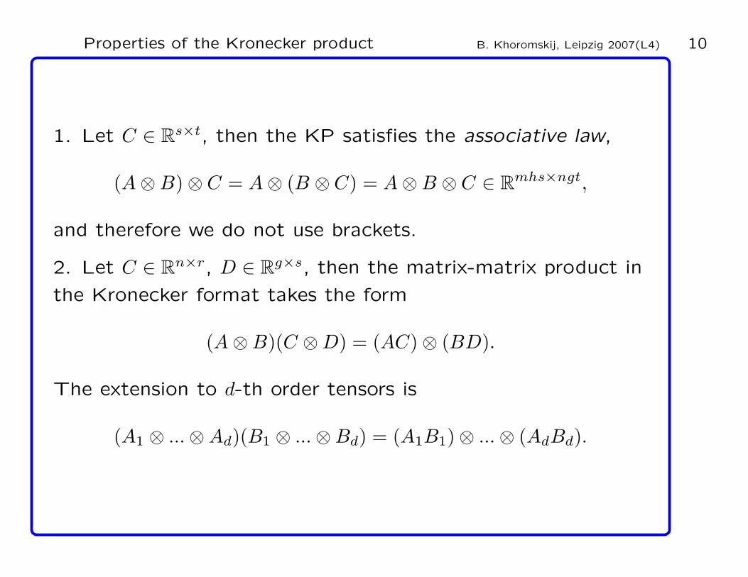
1. Let C ∈ Rs×t, then the KP satisfies the associative law,

(A ⊗ B) ⊗ C = A ⊗ (B ⊗ C) = A ⊗ B ⊗ C ∈ Rmhs×ngt,

and therefore we do not use brackets.

2. Let C ∈ Rn×r, D ∈ R

g×s, then the matrix-matrix product in

the Kronecker format takes the form

(A ⊗ B)(C ⊗ D) = (AC) ⊗ (BD).

The extension to d-th order tensors is

(A1 ⊗ ... ⊗ Ad)(B1 ⊗ ... ⊗ Bd) = (A1B1) ⊗ ... ⊗ (AdBd).

Properties of the Kronecker product B. Khoromskij, Leipzig 2007(L4) 11

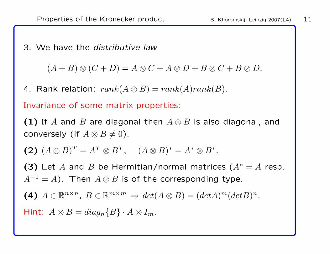
3. We have the distributive law

(A + B) ⊗ (C + D) = A ⊗ C + A ⊗ D + B ⊗ C + B ⊗ D.

4. Rank relation: rank(A ⊗ B) = rank(A)rank(B).

Invariance of some matrix properties:

(1) If A and B are diagonal then A ⊗ B is also diagonal, and

conversely (if A ⊗ B 6= 0).

(2) (A ⊗ B)T = AT ⊗ BT , (A ⊗ B)∗ = A∗ ⊗ B∗.

(3) Let A and B be Hermitian/normal matrices (A∗ = A resp.

A−1 = A). Then A ⊗ B is of the corresponding type.

(4) A ∈ Rn×n, B ∈ Rm×m ⇒ det(A ⊗ B) = (detA)m(detB)n.

Hint: A ⊗ B = diagnB · A ⊗ Im.

Matrix operations with the Kronecker product B. Khoromskij, Leipzig 2007(L4) 12

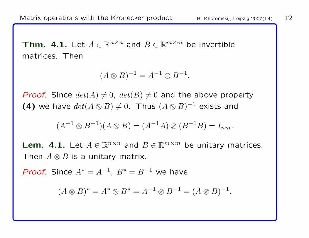
Thm. 4.1. Let A ∈ Rn×n and B ∈ R

m×m be invertible

matrices. Then

(A ⊗ B)−1 = A−1 ⊗ B−1.

Proof. Since det(A) 6= 0, det(B) 6= 0 and the above property

(4) we have det(A ⊗ B) 6= 0. Thus (A ⊗ B)−1 exists and

(A−1 ⊗ B−1)(A ⊗ B) = (A−1A) ⊗ (B−1B) = Inm.

Lem. 4.1. Let A ∈ Rn×n and B ∈ R

m×m be unitary matrices.

Then A ⊗ B is a unitary matrix.

Proof. Since A∗ = A−1, B∗ = B−1 we have

(A ⊗ B)∗ = A∗ ⊗ B∗ = A−1 ⊗ B−1 = (A ⊗ B)−1.

Matrix operations with the Kronecker product B. Khoromskij, Leipzig 2007(L4) 13

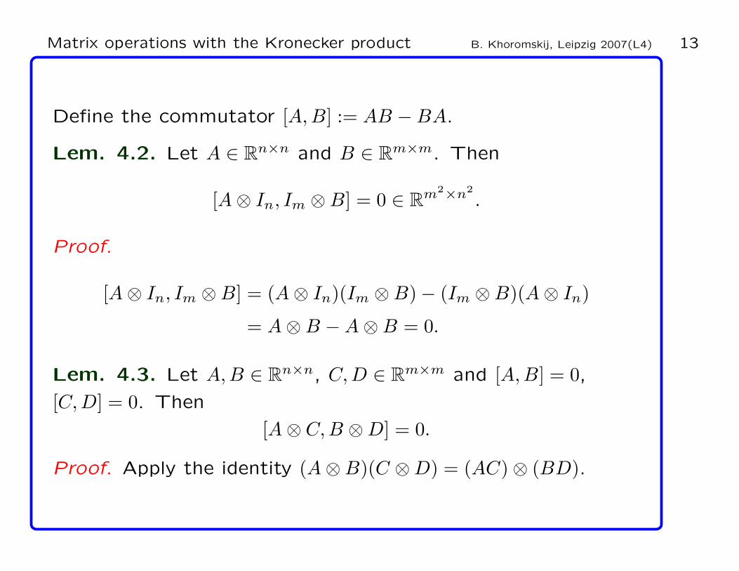
Define the commutator [A, B] := AB − BA.

Lem. 4.2. Let A ∈ Rn×n and B ∈ R

m×m. Then

[A ⊗ In, Im ⊗ B] = 0 ∈ Rm2×n2

.

Proof.

[A ⊗ In, Im ⊗ B] = (A ⊗ In)(Im ⊗ B) − (Im ⊗ B)(A ⊗ In)

= A ⊗ B − A ⊗ B = 0.

Lem. 4.3. Let A, B ∈ Rn×n, C, D ∈ R

m×m and [A, B] = 0,

[C, D] = 0. Then

[A ⊗ C, B ⊗ D] = 0.

Proof. Apply the identity (A ⊗ B)(C ⊗ D) = (AC) ⊗ (BD).

Matrix operations with the Kronecker product B. Khoromskij, Leipzig 2007(L4) 14

Lem. 4.4. Let A ∈ Rn×n and B ∈ R

m×m. Then

tr(A ⊗ B) = tr(A)tr(B).

Proof. Since diag(aiiB) = aiidiag(B), we have

tr(A ⊗ B) =n∑

i=1

m∑

j=1

aiibjj =n∑

i=1

aii

m∑

j=1

bjj .

Thm. 4.2. Let A, B, I ∈ Rn×n. Then

exp(A ⊗ I + I ⊗ B) = (expA) ⊗ (expB).

Proof. Since [A ⊗ I, I ⊗ B] = 0, we have

exp(A ⊗ I + I ⊗ B) = exp(A ⊗ I) exp(I ⊗ B).

Matrix operations with the Kronecker product B. Khoromskij, Leipzig 2007(L4) 15

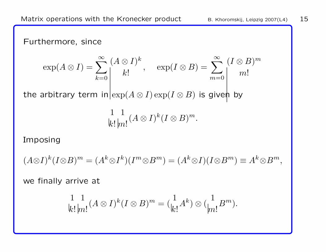
Furthermore, since

exp(A ⊗ I) =∞∑

k=0

(A ⊗ I)k

k!, exp(I ⊗ B) =

∞∑

m=0

(I ⊗ B)m

m!

the arbitrary term in exp(A ⊗ I) exp(I ⊗ B) is given by

1

k!

1

m!(A ⊗ I)k(I ⊗ B)m.

Imposing

(A⊗I)k(I⊗B)m = (Ak⊗Ik)(Im⊗Bm) = (Ak⊗I)(I⊗Bm) ≡ Ak⊗Bm,

we finally arrive at

1

k!

1

m!(A ⊗ I)k(I ⊗ B)m = (

1

k!Ak) ⊗ (

1

m!Bm).

Matrix operations with the Kronecker product B. Khoromskij, Leipzig 2007(L4) 16

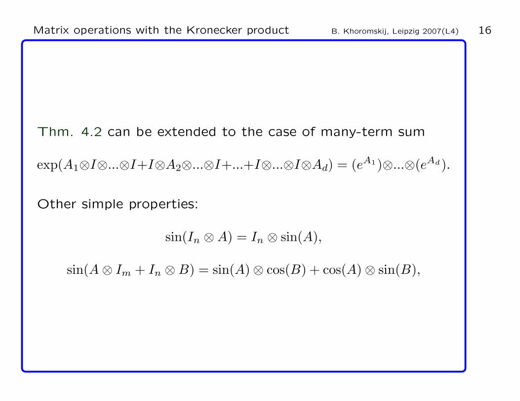
Thm. 4.2 can be extended to the case of many-term sum

exp(A1⊗I⊗...⊗I+I⊗A2⊗...⊗I+...+I⊗...⊗I⊗Ad) = (eA1)⊗...⊗(eAd).

Other simple properties:

sin(In ⊗ A) = In ⊗ sin(A),

sin(A ⊗ Im + In ⊗ B) = sin(A) ⊗ cos(B) + cos(A) ⊗ sin(B),

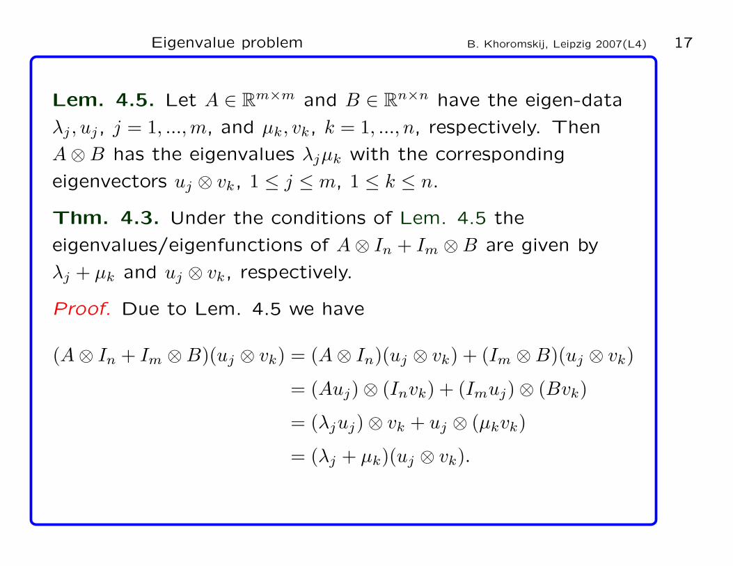
Eigenvalue problem B. Khoromskij, Leipzig 2007(L4) 17

Lem. 4.5. Let A ∈ Rm×m and B ∈ R

n×n have the eigen-data

λj , uj, j = 1, ..., m, and µk, vk, k = 1, ..., n, respectively. Then

A ⊗ B has the eigenvalues λjµk with the corresponding

eigenvectors uj ⊗ vk, 1 ≤ j ≤ m, 1 ≤ k ≤ n.

Thm. 4.3. Under the conditions of Lem. 4.5 the

eigenvalues/eigenfunctions of A ⊗ In + Im ⊗ B are given by

λj + µk and uj ⊗ vk, respectively.

Proof. Due to Lem. 4.5 we have

(A ⊗ In + Im ⊗ B)(uj ⊗ vk) = (A ⊗ In)(uj ⊗ vk) + (Im ⊗ B)(uj ⊗ vk)

= (Auj) ⊗ (Invk) + (Imuj) ⊗ (Bvk)

= (λjuj) ⊗ vk + uj ⊗ (µkvk)

= (λj + µk)(uj ⊗ vk).

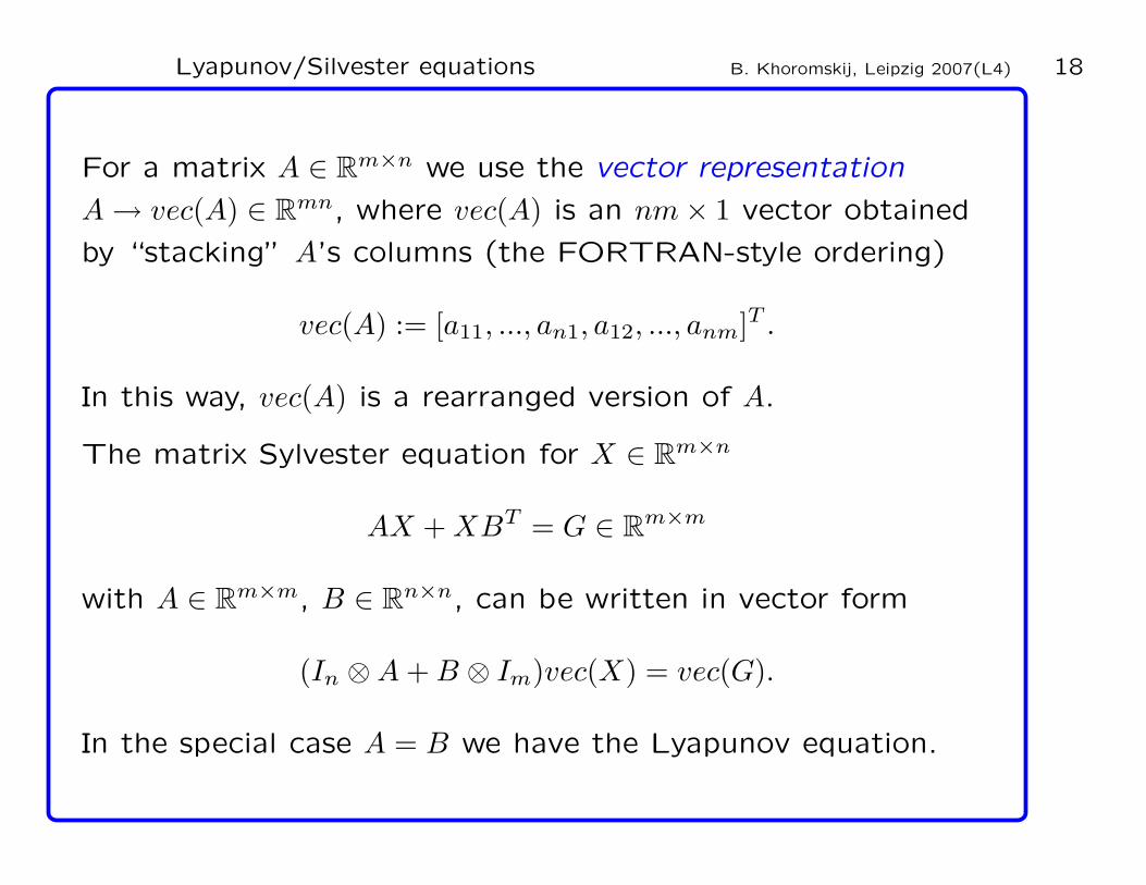
Lyapunov/Silvester equations B. Khoromskij, Leipzig 2007(L4) 18

For a matrix A ∈ Rm×n we use the vector representation

A → vec(A) ∈ Rmn, where vec(A) is an nm × 1 vector obtained

by “stacking” A’s columns (the FORTRAN-style ordering)

vec(A) := [a11, ..., an1, a12, ..., anm]T .

In this way, vec(A) is a rearranged version of A.

The matrix Sylvester equation for X ∈ Rm×n

AX + XBT = G ∈ Rm×m

with A ∈ Rm×m, B ∈ R

n×n, can be written in vector form

(In ⊗ A + B ⊗ Im)vec(X) = vec(G).

In the special case A = B we have the Lyapunov equation.

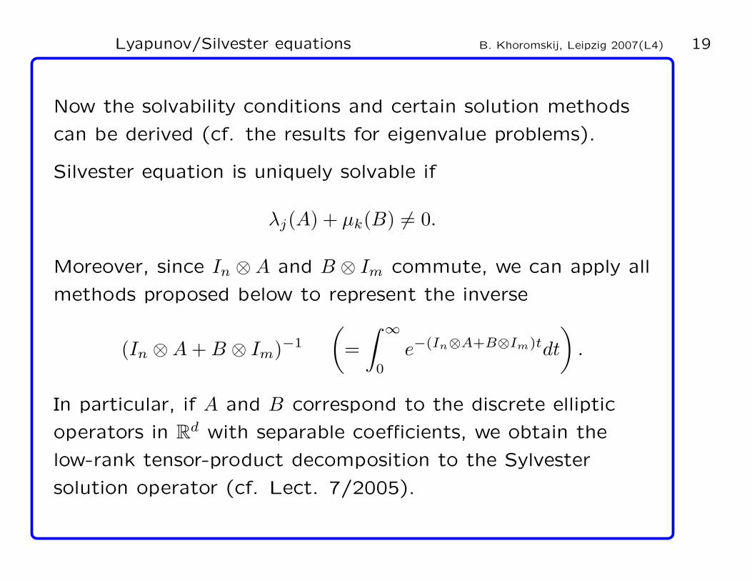
Lyapunov/Silvester equations B. Khoromskij, Leipzig 2007(L4) 19

Now the solvability conditions and certain solution methods

can be derived (cf. the results for eigenvalue problems).

Silvester equation is uniquely solvable if

λj(A) + µk(B) 6= 0.

Moreover, since In ⊗ A and B ⊗ Im commute, we can apply all

methods proposed below to represent the inverse

(In ⊗ A + B ⊗ Im)−1

(

=

∫ ∞

0

e−(In⊗A+B⊗Im)tdt

)

.

In particular, if A and B correspond to the discrete elliptic

operators in Rd with separable coefficients, we obtain the

low-rank tensor-product decomposition to the Sylvester

solution operator (cf. Lect. 7/2005).

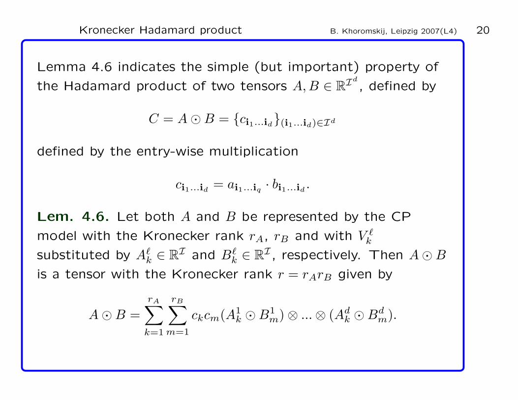
Kronecker Hadamard product B. Khoromskij, Leipzig 2007(L4) 20

Lemma 4.6 indicates the simple (but important) property of

the Hadamard product of two tensors A, B ∈ RId

, defined by

C = A ⊙ B = ci1...id(i1...id)∈Id

defined by the entry-wise multiplication

ci1...id = ai1...iq · bi1...id .

Lem. 4.6. Let both A and B be represented by the CP

model with the Kronecker rank rA, rB and with V ℓk

substituted by Aℓk ∈ R

I and Bℓk ∈ R

I, respectively. Then A ⊙ B

is a tensor with the Kronecker rank r = rArB given by

A ⊙ B =

rA∑

k=1

rB∑

m=1

ckcm(A1k ⊙ B1

m) ⊗ ... ⊗ (Adk ⊙ Bd

m).

Kronecker Hadamard product B. Khoromskij, Leipzig 2007(L4) 21

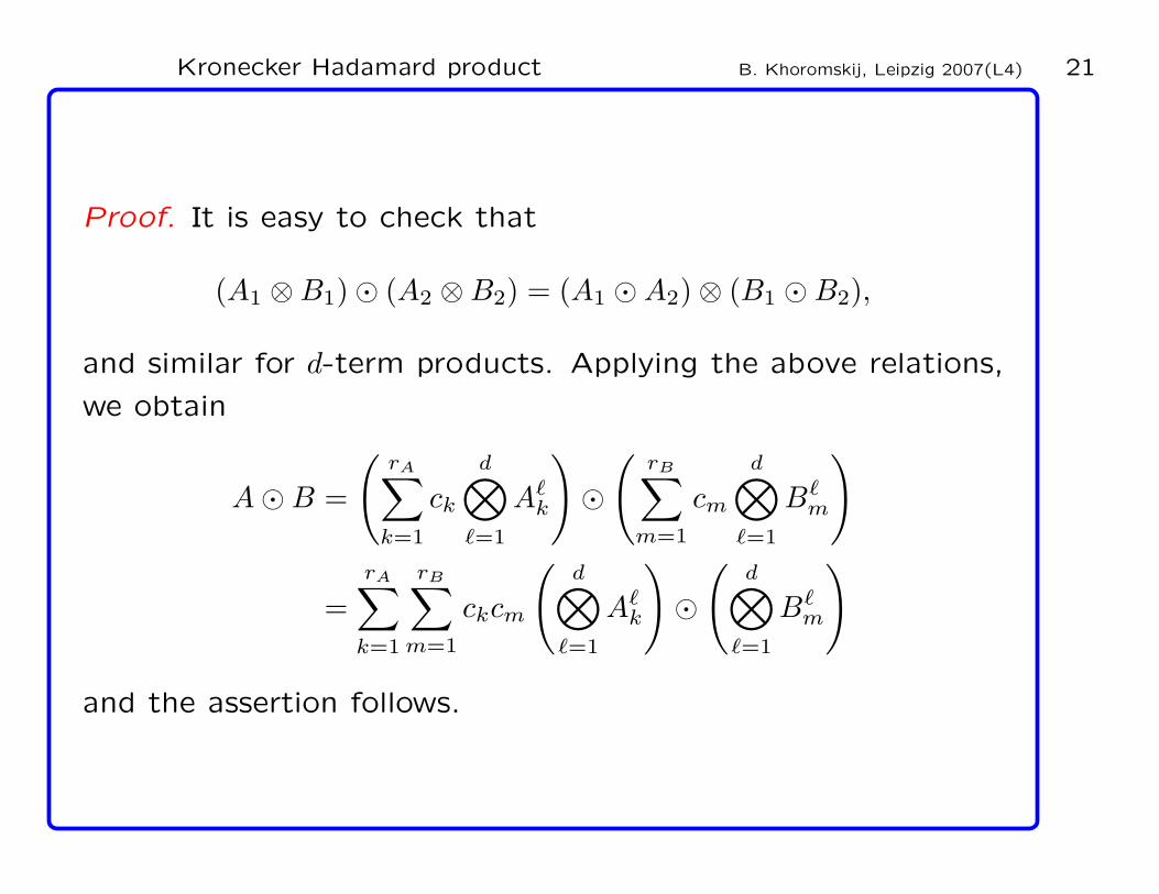
Proof. It is easy to check that

(A1 ⊗ B1) ⊙ (A2 ⊗ B2) = (A1 ⊙ A2) ⊗ (B1 ⊙ B2),

and similar for d-term products. Applying the above relations,

we obtain

A ⊙ B =

(

rA∑

k=1

ck

d⊗

ℓ=1

Aℓk

)

⊙

(

rB∑

m=1

cm

d⊗

ℓ=1

Bℓm

)

=

rA∑

k=1

rB∑

m=1

ckcm

(

d⊗

ℓ=1

Aℓk

)

⊙

(

d⊗

ℓ=1

Bℓm

)

and the assertion follows.

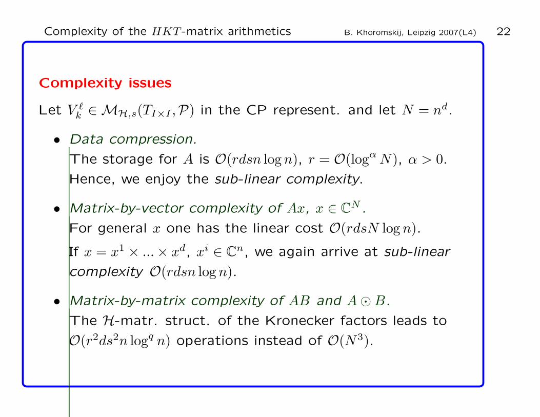
Complexity of the HKT -matrix arithmetics B. Khoromskij, Leipzig 2007(L4) 22

Complexity issues

Let V ℓk ∈ MH,s(TI×I ,P) in the CP represent. and let N = nd.

• Data compression.

The storage for A is O(rdsn log n), r = O(logα N), α > 0.

Hence, we enjoy the sub-linear complexity.

• Matrix-by-vector complexity of Ax, x ∈ CN .

For general x one has the linear cost O(rdsN log n).

If x = x1 × ... × xd, xi ∈ Cn, we again arrive at sub-linear

complexity O(rdsn log n).

• Matrix-by-matrix complexity of AB and A ⊙ B.

The H-matr. struct. of the Kronecker factors leads to

O(r2ds2n logq n) operations instead of O(N3).

How to construct a Kronecker product ? B. Khoromskij, Leipzig 2007(L4) 23

1. d = 2: SVD and ACA methods in the case of two-fold

decompositions.

2. d ≥ 2: Analytic approximation for the function-related d-th

order tensors (consider in Lect. 5).

Def. 4.2. Given the multi-variate function

g : Ω ∈ Rd → R with d = dp, p, d ∈ N, d ≥ 2,

Ω = (ζ1, ..., ζd) ∈ Rd : ‖ζℓ‖∞ ≤ L, ℓ = 1, ..., d ∈ R

d, L > 0,

where ‖ · ‖∞ means the ℓ∞-norm of ζℓ ∈ Rp (p = 1).

Introduce the function-generated d-th order tensor

A ≡ A(g) := [ai1...id ] ∈ RId

with ai1...id := g(ζ1i1

, ..., ζdid

). (1)

Approximation tools: sinc-methods, exponential fitting.

How to construct a Kronecker product ? B. Khoromskij, Leipzig 2007(L4) 24

3. d ≥ 3: Algebraic recompression methods:

3A. Greedy algorithms with dictionary

D :=

V (1) ×2 V (2)... ×d V (d) : V (ℓ) ∈ Rn, ‖V (ℓ)‖ = 1

.

(a) Fit the original tensor A by a rank-one tensor A1;

(b) Subtract A1 from the original tensor A;

(c) Approx. the residue A − A1 with another rank-one tensor.

For best rank-1 appr. one solves the minimisation problem

min ||A − V (1) ⊗ · · · ⊗ V (d)||F , V (ℓ) ∈ Rn

pℓ ,

by using ALS or the Newton iteration (proven convergence).

In general, convergence theory for Greedy algorithm is still

open question (see Lect.1).

How to construct a Kronecker product ? B. Khoromskij, Leipzig 2007(L4) 25

Def. 4.3. A tensor A ∈ Cr is orthogonally decomposable if

(V(ℓ)k , V

(ℓ)k′ ) = δk,k′ (k, k′ = 1, ..., r; ℓ = 1, ..., d).

Thm. 4.5. (Zhang, Golub) If a tensor of order d ≥ 3 is

orthogonally decomposable, then this decomposition is

unique, and the OGA correctly computes it.

Proof: See Lect. 1.

(3B) The Newton algorithm to solve the Lagrange eq. in the

constrained minimisation: Find A ∈ Cr and λ(k,ℓ) ∈ R s.t.

f(A) := ‖A − A0‖2F +

r∑

k=1

d∑

ℓ=1

λ(k,ℓ)(

‖V(ℓ)k ‖2 − 1

)

→ min. (2)

Efficient implementation of the Newton algorithm (M. Espig,

MPI MIS).

How to construct a Kronecker product ? B. Khoromskij, Leipzig 2007(L4) 26

(3C) Alternating least-squares (ALS).

Mode per mode components update, fix all V(ℓ), ℓ 6= m

(m = 1, ..., d).

Convergence theory only for r = 1 (Golub, Zhang; Kolda ’01)

Under certain simplifications, the constraint ALS

minimisation algorithm can be implemented in

O(m2n + Kitdr2m) op. (see Lect. 5).

The convergence theory behind these algorithms is not

complete, moreover the solution might not be unique or even

might not exist.

Summary I B. Khoromskij, Leipzig 2007(L4) 27

Motivation:

Basic linear algebra can be performed using one-dimensional

operations, thus avoiding the exponential scaling in d.

Bottleneck:

Lack of finite algebraic methods for the robust multi-fold

Kronecker decomposition of high order tensors (for d ≥ 3).

Difficulties with recompression in matrix operations. There

are efficient and robust ALS/Newton algorithms.

Observation:

Analytic approximation methods are of principal importance.

Classical example: an approximation by Gaussians.

Recent proposals: Sinc meth., exponential fitting, sparse

grids.