energies

Article

Effects of Increased Wind Power Generation onMid-Norway’s Energy Balance under Climate Change:A Market Based Approach

Baptiste François 1,*,†, Sara Martino 2, Lena S. Tøfte 2, Benoit Hingray 1, Birger Mo 2

and Jean-Dominique Creutin 1

1 Université Grenoble Alpes, CNRS, IGE, F-38000 Grenoble, France;benoit.hingray@univ-grenoble-alpes.fr (B.H.); jean-dominique.creutin@univ-grenoble-alpes.fr (J.-D.C.)

2 SINTEF Energy Research, 7465 Trondheim, Norway; sara.martino@sintef.no (S.M.);lena.s.tofte@sintef.no (L.S.T.); birger.mo@sintef.no (B.M.)

* Correspondence: bfrancois@umass.edu† Current address: Department of Civil and Environmental Engineering, University of Massachusetts

Amherst, Amherst, MA 01003-9303, USA.

Academic Editor: Robert LundmarkReceived: 25 November 2016; Accepted: 8 February 2017; Published: 15 February 2017

Abstract: Thanks to its huge water storage capacity, Norway has an excess of energy generation atannual scale, although significant regional disparity exists. On average, the Mid-Norway regionhas an energy deficit and needs to import more electricity than it exports. We show that this energydeficit can be reduced with an increase in wind generation and transmission line capacity, even infuture climate scenarios where both mean annual temperature and precipitation are changed. For theconsidered scenarios, the deficit observed in winter disappears, i.e., when electricity consumptionand prices are high. At the annual scale, the deficit behaviour depends more on future changes inprecipitation. Another consequence of changes in wind production and transmission capacity is themodification of electricity exchanges with neighbouring regions which are also modified both interms of average, variability and seasonality.

Keywords: variable renewable energy; wind; hydro; energy balance; energy market

1. Introduction

The United Nations Framework Convention on Climate Change (UNFCCC) Paris Agreementpromotes the transition to low carbon economy by replacing conventional by renewable energies suchas wind-, solar-, and hydro-power. In Europe, optimistic scenario by the European Climate Foundationforesees 100% renewable energy supply at the horizon 2050 [1]. Some countries such as Sweden,Spain and Austria are already well engaged for reaching this objective even before this deadline [2].This issue is also relevant at regional scale level as highlighted in Northern Italy by reference (Ref.) [3].

Thanks to its huge resources, Norwegian electricity generation already comes for about 95.3% fromhydropower [4]. Norway has an excess of energy at annual scale and presents on average a positivebalance between importation and exportation [5]. On account for its high water storage capacity,Norwegian reservoirs are sometimes considered as the future Blue Battery of Europe. Gullberg [6],for instance, explains that thanks to its actual hydropower capacity, Norway might balance powerin Europe. In the longer term, new transmission lines and pumped-storage hydropower in Norwaywould provide a backup capacity to the expected future high solar and wind power capacity inEurope [6,7].

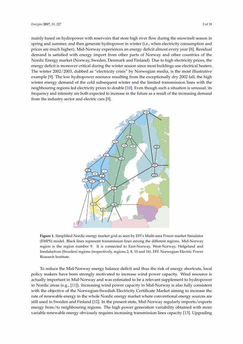
The positive energy balance for Norway hides significant regional disparities. Mid-Norway is themost illustrative example (region 9 on Figure 1). Like the rest of the country, its electricity system is

Energies 2017, 10, 227; doi:10.3390/en10020227 www.mdpi.com/journal/energies

Energies 2017, 10, 227 2 of 18

mainly based on hydropower with reservoirs that store high river flow during the snowmelt season inspring and summer, and then generate hydropower in winter (i.e., when electricity consumption andprices are much higher). Mid-Norway experiences an energy deficit almost every year [8]. Residualdemand is satisfied with energy import from other parts of Norway and other countries of theNordic Energy market (Norway, Sweden, Denmark and Finland). Due to high electricity prices, theenergy deficit is moreover critical during the winter season since most buildings use electrical heaters.The winter 2002/2003, dubbed as “electricity crisis” by Norwegian media, is the most illustrativeexample [9]. The low hydropower resource resulting from the exceptionally dry 2002 fall, the highwinter energy demand of the cold subsequent winter and the limited transmission lines with theneighbouring regions led electricity prices to double [10]. Even though such a situation is unusual, itsfrequency and intensity are both expected to increase in the future as a result of the increasing demandfrom the industry sector and electric cars [9].

Energies 2017, 10, 227 2 of 18

The positive energy balance for Norway hides significant regional disparities. Mid-Norway is the most illustrative example (region 9 on Figure 1). Like the rest of the country, its electricity system is mainly based on hydropower with reservoirs that store high river flow during the snowmelt season in spring and summer, and then generate hydropower in winter (i.e., when electricity consumption and prices are much higher). Mid-Norway experiences an energy deficit almost every year [8]. Residual demand is satisfied with energy import from other parts of Norway and other countries of the Nordic Energy market (Norway, Sweden, Denmark and Finland). Due to high electricity prices, the energy deficit is moreover critical during the winter season since most buildings use electrical heaters. The winter 2002/2003, dubbed as “electricity crisis” by Norwegian media, is the most illustrative example [9]. The low hydropower resource resulting from the exceptionally dry 2002 fall, the high winter energy demand of the cold subsequent winter and the limited transmission lines with the neighbouring regions led electricity prices to double [10]. Even though such a situation is unusual, its frequency and intensity are both expected to increase in the future as a result of the increasing demand from the industry sector and electric cars [9].

Figure 1. Simplified Nordic energy market grid as seen by EFI’s Multi-area Power market Simulator (EMPS) model. Black lines represent transmission lines among the different regions. Mid-Norway region is the region number 9. It is connected to East-Norway, West-Norway, Helgeland and Inndalselven (Sweden) regions (respectively, regions 2, 8, 10 and 16). EFI: Norwegian Electric Power Research Institute.

To reduce the Mid-Norway energy balance deficit and thus the risk of energy shortcuts, local policy makers have been strongly motivated to increase wind power capacity. Wind resource is actually important in Mid-Norway and was estimated to be a relevant supplement to hydropower in Nordic areas (e.g., [11]). Increasing wind power capacity in Mid-Norway is also fully consistent with the objective of the Norwegian-Swedish Electricity Certificate Market aiming to increase the rate of renewable energy in the whole Nordic energy market where conventional energy sources are still used in Sweden and Finland [12]. In the present state, Mid-Norway regularly imports/exports energy from/to neighbouring regions. The high power generation variability obtained with more variable renewable energy obviously requires increasing transmission lines capacity [13]. Upgrading transmission lines is planned between Mid-Norway and West-Norway (http://www.statnett.no). As highlighted during a stakeholder meeting organized for the region within the COMPLEX EU research project (http://owsgip.itc.utwente.nl/projects/complex/), public acceptance for wind power and transmission development is however not straightforward. It is high if the benefits from the project mainly go to the regional industry and trade development. It is however rather low if the generated power has to be exported to neighbouring regions.

Figure 1. Simplified Nordic energy market grid as seen by EFI’s Multi-area Power market Simulator(EMPS) model. Black lines represent transmission lines among the different regions. Mid-Norwayregion is the region number 9. It is connected to East-Norway, West-Norway, Helgeland andInndalselven (Sweden) regions (respectively, regions 2, 8, 10 and 16). EFI: Norwegian Electric PowerResearch Institute.

To reduce the Mid-Norway energy balance deficit and thus the risk of energy shortcuts, localpolicy makers have been strongly motivated to increase wind power capacity. Wind resource isactually important in Mid-Norway and was estimated to be a relevant supplement to hydropowerin Nordic areas (e.g., [11]). Increasing wind power capacity in Mid-Norway is also fully consistentwith the objective of the Norwegian-Swedish Electricity Certificate Market aiming to increase therate of renewable energy in the whole Nordic energy market where conventional energy sources arestill used in Sweden and Finland [12]. In the present state, Mid-Norway regularly imports/exportsenergy from/to neighbouring regions. The high power generation variability obtained with morevariable renewable energy obviously requires increasing transmission lines capacity [13]. Upgrading

Energies 2017, 10, 227 3 of 18

transmission lines is planned between Mid-Norway and West-Norway (http://www.statnett.no).As highlighted during a stakeholder meeting organized for the region within the COMPLEX EUresearch project (http://owsgip.itc.utwente.nl/projects/complex/), public acceptance for wind powerand transmission development is however not straightforward. It is high if the benefits from theproject mainly go to the regional industry and trade development. It is however rather low if thegenerated power has to be exported to neighbouring regions.

The first aim of the present work is to assess the effect of the development of additional windfarms and of the development of a new transmission line on the energy balance of Mid-Norway. Next,it is to explore the alternative question raised by local stakeholders about the finality of wind powerdevelopment—deficit limitation or export growth?

The second main objective of this study is to assess the ability of the Mid-Norway system to copewith a modification of the energy balance due to climate change. Climate change could first impact themean energy production via changes in wind- and hydro-power potential. In Nordic countries, changein wind power potential is expected to be very small with a lower than 5% decrease (a strong agreementwas obtained between Global Circulation Models (GCMs) as highlighted by Ref. [14]. Changes inhydropower potential are conversely expected to be quite large as a result of both precipitation andtemperature increase. The significant increase in precipitation expected for the region [15] shouldactually lead to an increase in river flows. Regional warming should additionally modify hydrologicalregimes with shorter winter droughts, earlier and smaller snowmelt flows [16]. On the other hand,climate change could also modify the electricity demand. Regional warming should especially lead toless heating needs in winter and to reduce the demand seasonality. The sensitivity of Mid-Norwaysystem performance to changes in mean precipitation and temperature is thus definitively importantto analyse.

Our analysis is carried out with the decision scaling approach developed by Ref. [17].This approach is based on sensitivity analyses of system responses to a set of synthetic climatechange scenarios. In the present study, we consider changes in mean precipitation and temperature.The objective is to build Climate Response Functions (hereafter noted as CRFs) putting inperspective: (i) either a given statistics of interest or an indicator of success of the consideredsystem obtained via a set of synthetic scenarios implemented with a sensitivity analyses of its drivers(i.e., in our case, temperature and precipitation variables); and (ii) the expected changes of the driversobtained from GCMs.

We use the EMPS (EFI’s Multi-area Power market Simulator, EFI: Norwegian Electric PowerResearch Institute) power market model for simulating the Nordic energy market for the presentand synthetic future climate scenarios and different wind power and transmission line capacities.The main indicator we account for is the one discussed by local stakeholders, namely the energybalance deficit in Mid-Norway. We focus on both the annual scale and the winter season.

The article is organized as follows. Section 2 gives the description of the Mid-Norway case studyand of the considered future Mid-Norway electricity system scenario. Section 3 details the databaseand models used. Section 4 illustrates current situation in Mid-Norway while Sections 5 and 6 giveresults obtained for future electricity system and future climate. Section 7 concludes and gives somehighlights for further research.

2. Case Study

All Nordic countries have liberalized their electricity markets, opening both electricity tradingand electricity production to competition. For a given region, this means that regional electricity pricesare determined by the energy balance and exchange capacity from/to neighbouring regions.

The Mid-Norway region covers the counties Møre og Romsdal, Sør-Trøndelag and most ofNord-Trøndelag. The region includes a set of fjords and mountains with altitudes ranging from 0 to1700 m.a.s.l. The climate is relatively wet with annual precipitation ranging with the altitude from

Energies 2017, 10, 227 4 of 18

500 mm/year in coastal areas to 3000 mm/year in inland mountains. Temperature also varies alongthis climate transect with an annual average ranging from +7 to −6 ◦C according to altitude.

Watercourses range from small coastal waterways to major mountainous rivers in the east, wherecatchment areas with large hydropower reservoirs are located. The hydrological regime also movesfrom an Atlantic regime in coastal areas (i.e., major flows in late autumn and winter) to an Alpineregime in the inland areas (i.e., low winter flows and high flows in late spring and summer due tosnow melt and rainfall events). The period of snow accumulation lasts several months and the snowmelting period usually starts in late March in the lowland regions and in June in high elevation areas.

Primary activities such as agriculture, fishery and forestry play a role in all the counties.Engineering industry, woodworking factories, fish farming, shipping trade and food industry areother important activities in the region. Energy-intensive industries and petroleum activity have largedemand of electricity, which has increased over the last 20 years and probably will continue to do so.

The region produces on average 14 TWh per year and consumes about 21 TWh. Mid-Norwayregion continuously buys electricity from the Nordic market (http://www.Statnett.no). Its storagecapacity is about 8% of Norway’s total capacity which represents about one third of the annualconsumption in the region (i.e., 6.7 TWh).

When this study was initiated in 2014, Mid-Norway wind power capacity equalled 1090 MW.Additional 4552 MW was already under construction or close to be, while concessions for another1100 MW power capacity were asked (for details see: https://www.nve.no/). In this study, we considertwo wind power capacity configurations. The first considers the installed wind power capacity in2014 (hereafter, this scenario is denoted W1). The second one considers the additional planned andasked wind power capacity (meaning a total wind power capacity equal to 6742 MW, denoted as W2scenario). Even though all asked concessions might not be accepted, W2 scenario gives a good guessabout wind power capacity evolution.

Two transmission line scenarios are also considered. The first scenario, denoted as G1, considersthe current line capacity: Mid-Norway is connected with East-Norway, West-Norway, Helgeland andInndalselven (Sweden) regions (respectively, region 2, 8, 10 and 16 in Figure 1). The second scenario,denoted G2, takes into account the increased transmission line capacity which will be achieved betweenMid-Norway and West-Norway within the next few years (see, for example, http://www.statnett.no/).Corresponding transmission line capacities are given in Table 1.

Table 1. Transmission line capacity scenarios between the Mid-Norway and its four neighbouringregions. Numbers in brackets refer to the market areas on Figure 1.

Mid-Norway [9] East-Norway [2] West-Norway [8] Helgeland [10] Inndalselven [16]

Scenario G1 600 MW 500 MW 900 MW 1950 MWScenario G2 600 MW 2000 MW 900 MW 1950 MW

3. Data and Models

The meteorological years used as reference cover 1961–1982. Along this period, the Nordicenergy system has been evolving with, among other things, construction of many hydropower plantsand water reservoirs. For our analyses, we consider fixed system configurations (we disregardany evolution of the system state during the considered time period). The reference configurationcorresponds to the current one: for the whole Nordic market, the hydropower, wind-power andtransmission line capacities are those available in 2014.

3.1. Mid-Norway Energy Balance Modelling

The EMPS model is a hydrothermal optimization and simulation model used by most playersin the Nordic energy market for long and medium-term price forecasting, hydro scheduling,system and investment analysis. One of the main advantages of this model is that it includes

Energies 2017, 10, 227 5 of 18

a detailed representation of the hydro-system (i.e., power stations, reservoirs, diversions, etc.).The optimization aims at minimizing the overall system costs via a variant of the so-called water valuemethod (see Ref. [18] for an early reference and Ref. [19] for a recent one). This method aims to balancethe income related to the immediate use of stored water against the future income expected fromits later use. A mathematical description of both optimization and simulation stages within EMPSmodelling is given in Ref. [20].

In this study, the EMPS model is used to simulate consequences of increasing the capacity of:(i) wind power generation; and (ii) transmission lines in Mid-Norway region for the currentand a variety of future climates. The model is set up for the whole Nordic energy market, towhich Mid-Norway region belongs. The Nordic energy market is divided into 23 areas (Figure 1).Each area is characterized by transmission constraints and hydropower system properties.The different connections among areas reflect physical transmission lines. The Nordic energy marketincludes more than a thousand reservoirs and several hundred hydropower plants in more than50 different river systems.

In the considered set up of the EMPS model, input data are: (i) weekly unregulated waterdischarge time series for a set of river basins in each market area; and (ii) weekly wind power timeseries for each market area. EMPS model simulations are typically done for an ensemble of historicalweather years assumed to have equal probability. The weather years provide physically consistentweather scenarios (i.e., scenarios with consistent space/time correlation among surface weathervariables) and in turn physically consistent scenarios for the various hydro-meteorological variables(river discharges, wind, solar radiation, temperature) that affect the energy production, the demandand then the market balance.

Hydro-meteorological time series scenarios required for the climate change impact analysis areobtained with a pattern scaling approach from the observed time series available for the referenceperiod (e.g., [21–23]. This approach is expected to rather well preserve space/time correlationsbetween variables. In the present case, the pattern scaling is carried out on a weekly basis. For riverdischarge, each reference river basin for which unregulated discharge time series are required in EMPSis considered separately. Fifty-two weekly scale factors C are first estimated from hydro-meteorologicalsimulations forced with a set of future climate change scenarios indexed by i. They are then used toderive future discharge series from the observed ones as follows:

QFuture(w, y, k, i) = QObs(w, y, k)C(w, k, i) (1)

with QFuture(w, y, k, i) the weekly water discharge for the w-th week of year y and the k-th referenceriver basin; QObs is the observed weekly time series water discharge within the EMPS archive andC(w,k,i), k = 1–52 are the scaling factors of weekly river discharges for the 52 calendar weeks.

For each market area and each future climate scenario i, scaling factors C are the ratiosbetween future and present average regional runoff. Future regional runoff time series are obtainedvia hydrological simulation, for each grid cell of each market area, with a distributed versionof the GSM-Socont hydrological model [24] (Glacier and SnowMelt—Soil CONTribution model).This model simulates the snowpack dynamic (snow accumulation and melt), water abstractionfrom evapotranspiration, slow and rapid components of river flow from infiltrated and effectiverainfall respectively. For each climate change scenario i, future meteorological scenarios used for thehydrological simulation are obtained with the scaling approach. Historical time series of precipitationand temperatures are modified with a multiplicative (additive) perturbation prescribed from therelative (absolute) change in annual precipitation (temperature) (hereafter denoted as ∆P and ∆T,respectively). As described later, a number of climate change scenarios, in terms of change in meanannual precipitation and temperature, are considered.

Historical precipitation and temperature data comes from the European Climate Assessment& Dataset (ECAD, [25]) with a 0.25◦ space resolution. The hydrological model required thecalibration of some parameters. We use a unique set of parameters for all market areas. It was

Energies 2017, 10, 227 6 of 18

calibrated by comparing the EMPS discharge archive with the discharges simulated from historicalmeteorological data.

In EMPS, the energy demand is indexed by the temperature, showing higher consumption duringcold days. The energy demand is linked to a lesser extent to price dependent contracts. This linkis represented by an additional demand which activates only if the price is low enough. A typicalexample of price dependent contract is a boiler-power contract where the customer has an oil heaterconnected in parallel with an electrical heater which is only used when the price is low. At annualscale, this price dependent demand represents about 8% of the temperature dependent demand.For future scenarios, the demand is estimated on a weekly basis from future temperature, obtainedfrom the perturbation approach mentioned above, and from the energy price derived within EMPS forthe current simulation time step.

We compute the weekly wind power generation time series with the wind speed databaseNORA10 [26] (NOrwegian Reanalysis Archive). NORA10 is currently the best near-surface(i.e., 10 m altitude) wind speed reanalysis over Scandinavian countries with a 10 km2 space resolution.Wind speed data are available from 1957. We used the wind power generation model developed byRef. [27] at daily time step. This model considers a nonlinear relationship between wind speed u(m·s−1) and wind power generation, hereafter noted PW (MWh). Below a given threshold (3 m·s−1 inthis study), the wind speed is not sufficient to enable power generation. The power generation is thena third order polynomial function of wind speed and reaches the maximum wind turbine efficiency ata second threshold (13 m·s−1). Above a third threshold (25 m·s−1), the power generation has to bestopped in order to avoid any damages on the wind turbine. The 70 m altitude wind speed time seriesused for computing wind power time series were estimated from the 10 m altitude NORA10 windfollowing the scaling equation:

u1 = u2

(h1

h2

)α

(2)

with u1 and u2 the wind speeds (m·s−1) at the altitudes h1 and h2 (m), respectively. α is an air frictioncoefficient chosen equal to 1/7 (no dimension) [28]. Simulated daily wind power generation timeseries are then aggregated at weekly time scale.

3.2. Climate Response Functions

CRFs are expressed in a two dimensional climate change space defined from changes intemperature and precipitation. The climate change factors we considered range from −20% to +50%for precipitation (with 10% step) and from 0 to +6 ◦C for temperature (with 1 ◦C step) in regards withthe reference period 1961–1982. CRFs are built from the 8 × 7 hydro-climatic time series scenariosobtained for these climate change scenarios via the scaling approach presented in the previous section.The reference period corresponds to the scenario with no change in temperature (i.e., +0 ◦C) and nochange in precipitation (i.e., +0%).

Positioning on the CRFs the future projections of climate experiments available from the latestGCMs allows discussing the expected effects of climate change for different future predictionperiods. In the present case, changes in future annual precipitation and temperature are estimatedfrom the outputs of an ensemble of 23 GCM projections from CMIP5 experiments [29] (CoupledModel Intercomparison Project Phase 5). Using several GCM projections illustrates uncertainty onprecipitation and temperature changes over the next decades and its amplitude in regard to thestudied effects.

In recent studies, climate change factors for a given climate experiment are classically estimatedfrom the change of the raw climate model outputs between a future and a reference period. A limitationto the robust estimation of change factors is the critical role of multi-decadal variations in the evolutionof the climate system. These low-frequency variations, commonly termed as climate internal variability,can, temporarily, worsen, reduce or even reverse the long-term impact of climate change. Internalvariability was found to be a major source of uncertainty in climate projections for the coming decades,

Energies 2017, 10, 227 7 of 18

especially for regional precipitation (e.g., [30,31]). A robust estimate of expected changes actuallyrequires a noise-free estimate of the climate response from the modelling chains. In the present case,we estimate the climate response of each GCM using all data of the transient simulations availablefor the model (150 years from 1950 to 2099). For each GCM, a trend model is first fitted to the rawclimate projections following Ref. [32] (piece-wise linear function of time for precipitation and a 3rdorder polynomial trend for temperature). The expected change for any future period is obtained fromthe change between trend estimates obtained respectively for this period and for the reference timeperiod. We consider three future 20-year time periods: 2040–2059, 2060–2079 and 2080–2099.

Figure 2 shows annual temperature and precipitation changes expected in Mid-Norway for eachfuture period. Model uncertainty for precipitation changes is very large although a significant increaseis consistently foreseen; only one GCM gives a slight decrease in precipitation. Changes in temperatureare more univocal showing an increase along the century. Note however that the dispersion amongmodels grows with the projection time horizon.Energies 2017, 10, 227 7 of 18

Figure 2. Scatterplot of average changes in precipitation and temperature for 23 GCM projections between control period (1961–1982) and three future time periods (i.e., 2040–2059, 2060–2079, and 2080–2099).

4. Mid-Norway Energy Balance in the Current System

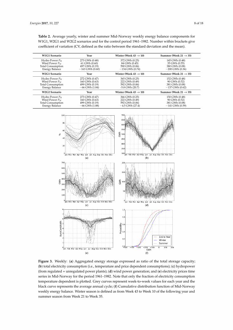
This section presents the results obtained by EMPS for the control configuration, i.e., with W1G1 scenario for the control climate (2014 wind power and transmission capacity, observed meteorological forcing). We first note that weekly wind and hydropower generation are much more variable than the demand (see coefficients of variation in Table 2). This result agrees with the literature related to the variability of renewable energies (e.g., [33]). In Mid-Norway, unregulated wind power generation is positively correlated with electricity consumption; the winter generation is higher than the summer one (Figure 3b,d). Mid-Norway reservoirs are handled so that stored inflows are mainly released during the winter season, making winter hydropower generation higher (see energy storage scheme and hydropower generation time series on Figure 3a,c). On average, the total production (i.e., sum of hydro and wind power) is not sufficient to supply the load, neither at yearly scale nor for winter and summer seasons (Table 2). As a result of the reservoirs’ management, the average energy balance deficit is higher in summer than in winter (Table 2). However, summer deficit is less critical than winter deficit since market prices are lower in summer (Figure 3e). For some years, electricity prices collapse, falling to 1 €cent/kWh during the spring and summer seasons. These situations correspond to periods where reservoirs are almost full and present a high risk of spill. When looking at the statistical distribution of the energy balance on Figure 3f, we note that only 10% of winter weeks present a positive energy balance while this number is lower than 5% during the summer season. Considering the whole year, less than 10% of all weeks have a positive energy balance.

Table 2. Average yearly, winter and summer Mid-Norway weekly energy balance components for W1G1, W2G1 and W2G2 scenarios and for the control period 1961–1982. Number within brackets give coefficient of variation (CV, defined as the ratio between the standard deviation and the mean).

W1G1 Scenario Year Winter (Week 43 → 10) Summer (Week 21 → 35) Hydro Power PH 273 GWh (0.48) 372 GWh (0.25) 145 GWh (0.48) Wind Power PW 61 GWh (0.60) 84 GWh (0.45) 35 GWh (0.55)

Total Consumption 497 GWh (0.19) 590 GWh (0.06) 380 GWh (0.08) Energy Balance −163 GWh (0.60) −134 GWh (0.74) −200 GWh (0.36) W2G1 Scenario Year Winter (Week 43 → 10) Summer (Week 21 → 35) Hydro Power PH 272 GWh (0.47) 365 GWh (0.25) 152 GWh (0.48) Wind Power PW 160 GWh (0.63) 222 GWh (0.49) 90 GWh (0.52)

Total Consumption 499 GWh (0.19) 592 GWh (0.06) 381 GWh (0.08) Energy Balance −66 GWh (1.84) -5.8 GWh (20.7) −137 GWh (0.62) W2G2 Scenario Year Winter (Week 43 → 10) Summer (Week 21 → 35) Hydro Power PH 273 GWh (0.47) 366 GWh (0.25) 150 GWh (0.48) Wind Power PW 160 GWh (0.63) 222 GWh (0.49) 90 GWh (0.52)

Total Consumption 499 GWh (0.19) 592 GWh (0.06) 381 GWh (0.08) Energy Balance −66 GWh (1.88) −4.5 GWh (27.4) −141 GWh (0.59)

Figure 2. Scatterplot of average changes in precipitation and temperature for 23 GCM projectionsbetween control period (1961–1982) and three future time periods (i.e., 2040–2059, 2060–2079,and 2080–2099).

4. Mid-Norway Energy Balance in the Current System

This section presents the results obtained by EMPS for the control configuration, i.e., with W1G1scenario for the control climate (2014 wind power and transmission capacity, observed meteorologicalforcing). We first note that weekly wind and hydropower generation are much more variable than thedemand (see coefficients of variation in Table 2). This result agrees with the literature related to thevariability of renewable energies (e.g., [33]). In Mid-Norway, unregulated wind power generation ispositively correlated with electricity consumption; the winter generation is higher than the summerone (Figure 3b,d). Mid-Norway reservoirs are handled so that stored inflows are mainly releasedduring the winter season, making winter hydropower generation higher (see energy storage schemeand hydropower generation time series on Figure 3a,c). On average, the total production (i.e., sum ofhydro and wind power) is not sufficient to supply the load, neither at yearly scale nor for winter andsummer seasons (Table 2). As a result of the reservoirs’ management, the average energy balance deficitis higher in summer than in winter (Table 2). However, summer deficit is less critical than winter deficitsince market prices are lower in summer (Figure 3e). For some years, electricity prices collapse, fallingto 1 €cent/kWh during the spring and summer seasons. These situations correspond to periods wherereservoirs are almost full and present a high risk of spill. When looking at the statistical distributionof the energy balance on Figure 3f, we note that only 10% of winter weeks present a positive energybalance while this number is lower than 5% during the summer season. Considering the whole year,less than 10% of all weeks have a positive energy balance.

Energies 2017, 10, 227 8 of 18

Table 2. Average yearly, winter and summer Mid-Norway weekly energy balance components forW1G1, W2G1 and W2G2 scenarios and for the control period 1961–1982. Number within brackets givecoefficient of variation (CV, defined as the ratio between the standard deviation and the mean).

W1G1 Scenario Year Winter (Week 43 → 10) Summer (Week 21 → 35)

Hydro Power PH 273 GWh (0.48) 372 GWh (0.25) 145 GWh (0.48)Wind Power PW 61 GWh (0.60) 84 GWh (0.45) 35 GWh (0.55)

Total Consumption 497 GWh (0.19) 590 GWh (0.06) 380 GWh (0.08)Energy Balance −163 GWh (0.60) −134 GWh (0.74) −200 GWh (0.36)

W2G1 Scenario Year Winter (Week 43 → 10) Summer (Week 21 → 35)

Hydro Power PH 272 GWh (0.47) 365 GWh (0.25) 152 GWh (0.48)Wind Power PW 160 GWh (0.63) 222 GWh (0.49) 90 GWh (0.52)

Total Consumption 499 GWh (0.19) 592 GWh (0.06) 381 GWh (0.08)Energy Balance −66 GWh (1.84) -5.8 GWh (20.7) −137 GWh (0.62)

W2G2 Scenario Year Winter (Week 43 → 10) Summer (Week 21 → 35)

Hydro Power PH 273 GWh (0.47) 366 GWh (0.25) 150 GWh (0.48)Wind Power PW 160 GWh (0.63) 222 GWh (0.49) 90 GWh (0.52)

Total Consumption 499 GWh (0.19) 592 GWh (0.06) 381 GWh (0.08)Energy Balance −66 GWh (1.88) −4.5 GWh (27.4) −141 GWh (0.59)

Energies 2017, 10, 227 8 of 18

(a) (b)

(c) (d)

(e) (f)

Figure 3. Weekly: (a) Aggregated energy storage expressed as ratio of the total storage capacity; (b) total electricity consumption (i.e., temperature and price dependent consumptions); (c) hydropower (from regulated + unregulated power plants); (d) wind power generation; and (e) electricity prices time series in Mid-Norway for the period 1961–1982. Note that only the fraction of electricity consumption temperature dependent is plotted. Grey curves represent week-to-week values for each year and the black curve represents the average annual cycle; (f) Cumulative distribution function of Mid-Norway weekly energy balance. Winter season is defined as from Week 43 to Week 10 of the following year and summer season from Week 21 to Week 35.

As a result of the deficit, Mid-Norway imports electricity from the regions of Inndalselven and Helgeland over, respectively, 90% and 70% of the weeks (Figure 4). Meanwhile, the region exports electricity to East-Norway 90% of the time. The line between Mid- and West-Norway is used for both importing and exporting electricity. Note that 20% of the weeks the transmission line is not used at all (Figure 4). Similar distributions are obtained during winter season. Note that these simulated results are consistent with the current deficit and exchange situation of the region as presented in the previous sections.

Figure 3. Weekly: (a) Aggregated energy storage expressed as ratio of the total storage capacity;(b) total electricity consumption (i.e., temperature and price dependent consumptions); (c) hydropower(from regulated + unregulated power plants); (d) wind power generation; and (e) electricity prices timeseries in Mid-Norway for the period 1961–1982. Note that only the fraction of electricity consumptiontemperature dependent is plotted. Grey curves represent week-to-week values for each year and theblack curve represents the average annual cycle; (f) Cumulative distribution function of Mid-Norwayweekly energy balance. Winter season is defined as from Week 43 to Week 10 of the following year andsummer season from Week 21 to Week 35.

Energies 2017, 10, 227 9 of 18

As a result of the deficit, Mid-Norway imports electricity from the regions of Inndalselven andHelgeland over, respectively, 90% and 70% of the weeks (Figure 4). Meanwhile, the region exportselectricity to East-Norway 90% of the time. The line between Mid- and West-Norway is used for bothimporting and exporting electricity. Note that 20% of the weeks the transmission line is not used atall (Figure 4). Similar distributions are obtained during winter season. Note that these simulatedresults are consistent with the current deficit and exchange situation of the region as presented in theprevious sections.

Energies 2017, 10, 227 9 of 18

(a)

(b)

Figure 4. Cumulative distribution functions of weekly energy exchanges between Mid-Norway and the neighbouring regions during: (a) the whole year; and (b) the winter season only. Negative (blue background) and positive (red background) values, respectively, show importation to and exportation from Mid-Norway. Note than only the line with West-Norway is reinforced in G2 scenario. Note that some distributions clearly show when the full capacity is reached for the whole week (e.g., East-Norway).

Figure 4. Cumulative distribution functions of weekly energy exchanges between Mid-Norway andthe neighbouring regions during: (a) the whole year; and (b) the winter season only. Negative(blue background) and positive (red background) values, respectively, show importation to andexportation from Mid-Norway. Note than only the line with West-Norway is reinforced in G2 scenario.Note that some distributions clearly show when the full capacity is reached for the whole week(e.g., East-Norway).

Energies 2017, 10, 227 10 of 18

5. Increasing Wind Power and Transmission Capacities

This section focuses on the evolution of the energy balance by considering, firstly, an increase ofwind power capacity in Mid-Norway (i.e., W2G1 scenario), and secondly, an increase of both windpower capacity and transmission line capacity between Mid- and West-Norway (i.e., W2G2 scenario).

Additional wind power capacity almost triples the average generation from 61 to 160 GWh perweek. The weekly generation increases from 84 to 222 GWh in winter season and from 35 to 90 GWhin summer (Table 2). Higher energy generation obviously reduces the energy balance deficit (Table 2).For winter, the deficit is close to 0 (i.e., −5.8 GWh/week). It remains rather important in summer(−137 GWh/week) as well as at annual scale (−66 GWh/week). Comparing W1G1 and W2G1scenarios, we note that, on average, Mid-Norway exports every week 2 GWh more, which correspondsto roughly 2% of the additional wind generation. In winter, average export reaches 10 GWh (about 7%of the additional generation at this season). One can note that this exported electricity could have beenused to further reduce Mid-Norway deficit.

Wind power generation being highly variable (see CV in Table 2), increasing wind powergeneration implies a higher temporal variability of the energy balance (the CV of the weekly energybalance increase by a factor of 3 during the whole year and by a factor 28 during the winterseason; Table 2). Such variability requires systematically more important energy exchanges betweenMid-Norway and all its neighbouring regions (Figure 4), even when the average deficit is close to 0as it is the case during the winter, for instance. Transmission lines are effectively more often used forexporting energy and they are more often used at full capacity. For instance, Mid-Norway exportsat full capacity to East-Norway during more than 25% of the weeks during the year (35% in winter).Another example is the number of winter weeks during which Mid-Norway exports electricity toWest-Norway (60% of the weeks for W2G1 against roughly 40% for W1G1).

The increased transmission capacity of the line between Mid- and West-Norway (i.e., W2G2scenario) has no significant effect on the mean annual deficit (Table 2). Note that the winter deficitslightly decreases to −4.5 GWh/week. Energy exchange distribution functions obtained with W2G2scenario roughly overlap the ones obtained with W2G1 except for the reinforced line (Figure 4).Although the increased capacity is only used about 10% and 15% of the time, it allows exporting animportant amount of energy. This mainly occurs during high wind power generation periods and/orwhen reservoirs are close to full in spring.

6. Evolution of Mid-Norway Energy Balance in a Changing Climate

This section focuses on climate change impact on Mid-Norway energy balance. As discussedin introduction, climate change is expected to impact both the average and the time variabilityof electricity generation and consumption. Considering changes in temperature and precipitation,two components of the energy balance are modified: the river flows and the electricity consumption.This section presents first the raw changes in these two components and secondly the impacts onMid-Norway energy balance and exchanges.

6.1. Climate Change Impacts on River Flows and Electricity Consumption

The main driver of change in river flow is precipitation; higher precipitation giving higher riverflows. As illustrated on Figure 5a, river flow increases linearly with precipitation change and highertemperatures increase evaporation and in turn reduce river flow. The effect of increasing temperatureon mean annual discharge is rather weak. For instance, river flows slightly increase up to ∆T equalto +2 ◦C and then decrease when temperatures rise above this threshold. In any case, river flowmodification is less than 5% whatever the change in temperature. However, increasing temperaturesignificantly reduces river flow seasonality with higher discharges values in winter (due to a higherratio of liquid precipitation resulting from higher temperatures) and lower values during the springand summer seasons (due to less snowpack; not shown). Annual temperature and precipitation

Energies 2017, 10, 227 11 of 18

changes provided by 23 GCMs are also plotted on Figure 5a for three different future time periods.The CRF shows anticipated changes in water discharge as a function of temperature and precipitationestimates for each future period and each GCM. For instance, accounting for changes in temperatureand precipitation obtained by most GCMs, future river flow would increase by 30% for the 2080–2099time period. Only one GCM shows a small decrease in average water discharges related with adecrease in precipitation.

Energies 2017, 10, 227 11 of 18

estimates for each future period and each GCM. For instance, accounting for changes in temperature and precipitation obtained by most GCMs, future river flow would increase by 30% for the 2080–2099 time period. Only one GCM shows a small decrease in average water discharges related with a decrease in precipitation.

Figure 5b shows the CRF obtained for the average annual electricity consumption. By construction, electricity consumption decreases almost linearly when temperature increases. Interestingly, increasing precipitation induces a slight increase of electricity consumption actually linked to price dependent contracts. More abundant water resource makes lower electricity prices (not shown) and stimulates consumption. Annual temperature changes obtained from the selected GCMs show a decrease in average electricity consumption, up to 8% for the time period 2080–2099.

(a) (b)

Figure 5. Climate Response Functions (CRFs) of the average annual changes (%) in: (a) river inflows; and (b) electricity consumption (obtained for W1G1 scenario) compared with control period. The dashed black curves show the “no change” edge. Dots show expected annual changes in temperature and precipitation change obtained from 23 GCM, as illustrated in Figure 2, for 2040–2059 (blue), 2060–2079 (green) and 2080–2099 (red).

6.2. Climate Change Impacts on Energy Balance and Exchanges in Mid-Norway

We only focus on differences between W1G1 and W2G2 scenarios considering that climate should change once wind power generation and transmission line capacity will be both developed.

Changes in water discharges and electricity consumption will modify the Mid-Norway energy balance deficit at both annual and winter season scales (Figure 6). Precipitation is the main factor of the deficit modification. Considering the current Mid-Norway electricity system (i.e., W1G1 scenario), the energy balance remains negative whatever the changes in precipitation and temperature. The energy balance might become positive during the winter season if changes in precipitation and temperature are quite drastic (from +40% to +50% in annual precipitation and from +4 to +6 °C in annual temperature).

When considering climate change with additional wind generation and stronger transmission lines (i.e., W2G2 scenario), the annual energy balance might become positive with less drastic changes than for the W1G1 scenario. For instance, the annual balance might become positive with 25% precipitation more and whatever the annual increase in temperature. Below 25% increase in precipitation, annual temperature must increase enough to reduce electricity consumption and to make the balance positive. For instance, an increase in annual temperature of +3.5 °C is required if precipitation increases by only 10%. During the winter season, the energy balance becomes positive but when precipitation decreases significantly or when a decrease in precipitation is conjugated with a low rise in temperature (which does not decrease significantly the electricity consumption). However, these two later configurations are not likely to appear according to GCMs projections as illustrated on Figure 6.

Figure 5. Climate Response Functions (CRFs) of the average annual changes (%) in: (a) riverinflows; and (b) electricity consumption (obtained for W1G1 scenario) compared with control period.The dashed black curves show the “no change” edge. Dots show expected annual changes intemperature and precipitation change obtained from 23 GCM, as illustrated in Figure 2, for 2040–2059(blue), 2060–2079 (green) and 2080–2099 (red).

Figure 5b shows the CRF obtained for the average annual electricity consumption. By construction,electricity consumption decreases almost linearly when temperature increases. Interestingly, increasingprecipitation induces a slight increase of electricity consumption actually linked to price dependentcontracts. More abundant water resource makes lower electricity prices (not shown) and stimulatesconsumption. Annual temperature changes obtained from the selected GCMs show a decrease inaverage electricity consumption, up to 8% for the time period 2080–2099.

6.2. Climate Change Impacts on Energy Balance and Exchanges in Mid-Norway

We only focus on differences between W1G1 and W2G2 scenarios considering that climate shouldchange once wind power generation and transmission line capacity will be both developed.

Changes in water discharges and electricity consumption will modify the Mid-Norway energybalance deficit at both annual and winter season scales (Figure 6). Precipitation is the main factor ofthe deficit modification. Considering the current Mid-Norway electricity system (i.e., W1G1 scenario),the energy balance remains negative whatever the changes in precipitation and temperature.The energy balance might become positive during the winter season if changes in precipitationand temperature are quite drastic (from +40% to +50% in annual precipitation and from +4 to +6 ◦C inannual temperature).

When considering climate change with additional wind generation and stronger transmission lines(i.e., W2G2 scenario), the annual energy balance might become positive with less drastic changes thanfor the W1G1 scenario. For instance, the annual balance might become positive with 25% precipitationmore and whatever the annual increase in temperature. Below 25% increase in precipitation, annualtemperature must increase enough to reduce electricity consumption and to make the balance positive.For instance, an increase in annual temperature of +3.5 ◦C is required if precipitation increases byonly 10%. During the winter season, the energy balance becomes positive but when precipitationdecreases significantly or when a decrease in precipitation is conjugated with a low rise in temperature

Energies 2017, 10, 227 12 of 18

(which does not decrease significantly the electricity consumption). However, these two laterconfigurations are not likely to appear according to GCMs projections as illustrated on Figure 6.Energies 2017, 10, 227 12 of 18

(a) (b)

(c) (d)

Figure 6. CRFs of the Mid-Norway weekly energy balance (GWh) obtained with the: (a) W1G1 scenario for the whole year; (b) W2G2 scenario for the whole year; (c) W1G1 scenario for the winter season; and (d) W2G2 scenario for the winter season. Nil energy balance curves are highlighted with dashed black lines. The coloured dots give temperature and precipitation changes from the 23 considered GCMs and three considered future time period (blue: 2040–2059; green: 2060–2079; and red: 2080–2099).

Changes in Mid-Norway energy balance deficit imply modifications of energy exchanges with the neighbouring regions. Energy imports from Helgeland should grow over the next decades (not shown). This results from both higher production in Helgeland (due to increasing precipitation) and lower consumption (due to higher temperatures; not shown). In association with higher in-situ generation, Mid-Norway region is able to export more electricity and then to strengthen its hub role in the Nordic energy market. As a consequence, electricity exports to East-Norway linearly increase with precipitation (and thus with hydropower generation) within Mid-Norway region (not shown). Note that East-Norway does not produce electricity. We note on Figure 7 that for both W1G1 and W2G2 scenarios, Mid-Norway keeps importing on average electricity from Inndalselven region at annual scale. However, thanks to the development of wind generation, the region might export more electricity to Inndalselven than it imports during the winter season (Figure 7). As discussed in the previous section, Mid-Norway imports and exports electricity from/to West-Norway, with a slightly negative balance, especially during the winter season. With the W2G2 scenario under future climate, exports from Mid-Norway to West-Norway are expected to increase significantly. We note that temperature changes impact average exportation from Mid-Norway to West-Norway more than the reinforcement of the line (Figure 7).

Figure 6. CRFs of the Mid-Norway weekly energy balance (GWh) obtained with the: (a) W1G1 scenariofor the whole year; (b) W2G2 scenario for the whole year; (c) W1G1 scenario for the winter season; and(d) W2G2 scenario for the winter season. Nil energy balance curves are highlighted with dashed blacklines. The coloured dots give temperature and precipitation changes from the 23 considered GCMs andthree considered future time period (blue: 2040–2059; green: 2060–2079; and red: 2080–2099).

Changes in Mid-Norway energy balance deficit imply modifications of energy exchanges withthe neighbouring regions. Energy imports from Helgeland should grow over the next decades (notshown). This results from both higher production in Helgeland (due to increasing precipitation)and lower consumption (due to higher temperatures; not shown). In association with higher in-situgeneration, Mid-Norway region is able to export more electricity and then to strengthen its hub rolein the Nordic energy market. As a consequence, electricity exports to East-Norway linearly increasewith precipitation (and thus with hydropower generation) within Mid-Norway region (not shown).Note that East-Norway does not produce electricity. We note on Figure 7 that for both W1G1 andW2G2 scenarios, Mid-Norway keeps importing on average electricity from Inndalselven region atannual scale. However, thanks to the development of wind generation, the region might exportmore electricity to Inndalselven than it imports during the winter season (Figure 7). As discussedin the previous section, Mid-Norway imports and exports electricity from/to West-Norway, with aslightly negative balance, especially during the winter season. With the W2G2 scenario under futureclimate, exports from Mid-Norway to West-Norway are expected to increase significantly. We notethat temperature changes impact average exportation from Mid-Norway to West-Norway more thanthe reinforcement of the line (Figure 7).

Energies 2017, 10, 227 13 of 18Energies 2017, 10, 227 13 of 18

Transmission line: Mid-Norway Inndalselven (Sweden) W1G1 W2G2

Transmission line: Mid-Norway West-Norway

Figure 7. CRFs of the Mid-Norway energy exchanges with: Inndalselven (Sweden) (top); and West-Norway (bottom). CRFs left and right columns are obtained with W1G1 and W2G2 scenarios respectively. For each transmission line, top CRFs are for the whole year and the bottom for the winter season. Nil energy balance curves are highlighted with dashed black lines. For more details, see Figure 6 caption.

Figure 7. CRFs of the Mid-Norway energy exchanges with: Inndalselven (Sweden) (top);and West-Norway (bottom). CRFs left and right columns are obtained with W1G1 and W2G2 scenariosrespectively. For each transmission line, top CRFs are for the whole year and the bottom for thewinter season. Nil energy balance curves are highlighted with dashed black lines. For more details,see Figure 6 caption.

Energies 2017, 10, 227 14 of 18

7. Discussion and Conclusions

Norwegian reservoirs are likely to be used as backup capacity for increasing wind and solarpower in Europe. However, important space variability exists and some regions show an importantenergy balance deficit such as Mid-Norway.

Using the EMPS model to simulate the Nordic energy market, we show that increasing windpower capacity in Mid-Norway can reduce the energy balance deficit. The deficit becomes almostnil during high consumption/price period, i.e., in winter, although the deficit remains importantat yearly scale (Table 2). Simulations also show that generation from new wind power plants inMid-Norway is almost totally used for reducing the deficit. Only 2% of the additional wind generationis exported during the whole year (7% during winter season). Such a result should please Mid-Norwaystakeholders about the finality of on-going wind power plant construction.

Increasing transmission line capacity between Mid- and West-Norway does not change drasticallythe export/import patterns from/to Mid-Norway. The increased capacity is actually used only fewtimes during the year (less than 15% of the weeks for exporting and less than 10% for importingelectricity; Figure 4). Although this increased capacity is not often used, it limits spillage when thereservoirs are full, in spring season especially.

Regarding climate change impact in Mid-Norway region, temperature is expected to rise inthe next decades as well as precipitation (only one GCM out of 23 gives a slight decrease ofannual precipitation; Figure 2). These changes have positive impact on Mid-Norway energy systemcomponents. More precipitation makes higher river flows and thus higher hydropower potential andhigher temperatures lead to lower electricity consumption.

We assess the joint effect of increasing wind and transmission capacities with climate changewith the Decision Scaling approach as developed by Ref. [17]. The Cumulative Distribution Functions(CDFs) of the weekly energy balance, calculated from changes in precipitation and temperature givenby the GCMs, are illustrated in Figure 8. For the considered GCMs, the average energy balance deficitshould decrease in time, highlighting that Mid-Norway climate will become increasingly favourableto the local balance between demand and generation. For instance, at annual scale, one third of theconsidered GCMs foresee an average positive balance during the 2060–2079 time period and two thirdsduring the 2080–2099 time period (Figure 8a).

Energies 2017, 10, 227 14 of 18

7. Discussion and Conclusions

Norwegian reservoirs are likely to be used as backup capacity for increasing wind and solar power in Europe. However, important space variability exists and some regions show an important energy balance deficit such as Mid-Norway.

Using the EMPS model to simulate the Nordic energy market, we show that increasing wind power capacity in Mid-Norway can reduce the energy balance deficit. The deficit becomes almost nil during high consumption/price period, i.e., in winter, although the deficit remains important at yearly scale (Table 2). Simulations also show that generation from new wind power plants in Mid-Norway is almost totally used for reducing the deficit. Only 2% of the additional wind generation is exported during the whole year (7% during winter season). Such a result should please Mid-Norway stakeholders about the finality of on-going wind power plant construction.

Increasing transmission line capacity between Mid- and West-Norway does not change drastically the export/import patterns from/to Mid-Norway. The increased capacity is actually used only few times during the year (less than 15% of the weeks for exporting and less than 10% for importing electricity; Figure 4). Although this increased capacity is not often used, it limits spillage when the reservoirs are full, in spring season especially.

Regarding climate change impact in Mid-Norway region, temperature is expected to rise in the next decades as well as precipitation (only one GCM out of 23 gives a slight decrease of annual precipitation; Figure 2). These changes have positive impact on Mid-Norway energy system components. More precipitation makes higher river flows and thus higher hydropower potential and higher temperatures lead to lower electricity consumption.

We assess the joint effect of increasing wind and transmission capacities with climate change with the Decision Scaling approach as developed by Ref. [17]. The Cumulative Distribution Functions (CDFs) of the weekly energy balance, calculated from changes in precipitation and temperature given by the GCMs, are illustrated in Figure 8. For the considered GCMs, the average energy balance deficit should decrease in time, highlighting that Mid-Norway climate will become increasingly favourable to the local balance between demand and generation. For instance, at annual scale, one third of the considered GCMs foresee an average positive balance during the 2060–2079 time period and two thirds during the 2080–2099 time period (Figure 8a).

(a) (b)

Figure 8: Cumulative distribution function (CDF) of the weekly energy balance for the whole year (GWh) (a) and for the winter season (b) calculated from annual changes in precipitation and temperature provided by GCMs (blue: 2040–2059; green: 2060–2079; red: 2080–2099). Vertical solid dotted, dashed and dotted black lines shows energy balance values obtained under present climate for W1G1, W2G1 and W2G2 scenarios, respectively. Note that for the whole year, CDFs of W2G1 and W2G2 scenarios are overlapping.

Figure 8. Cumulative distribution function (CDF) of the weekly energy balance for the wholeyear (GWh) (a) and for the winter season (b) calculated from annual changes in precipitation andtemperature provided by GCMs (blue: 2040–2059; green: 2060–2079; red: 2080–2099). Vertical soliddotted, dashed and dotted black lines shows energy balance values obtained under present climatefor W1G1, W2G1 and W2G2 scenarios, respectively. Note that for the whole year, CDFs of W2G1 andW2G2 scenarios are overlapping.

Energies 2017, 10, 227 15 of 18

Returning to the question that motivated this study, we conclude that coupling effects fromboth climate change and increasing wind power and transmission lines capacities appear to lead to awin-win situation: Mid-Norway average energy balance deficit is reduced and would become positivein the next decades allowing the region to increase its exportation, especially during winter seasonwhen prices are high.

To our knowledge, this work was the first attempt to applying the Decision Scaling approachto electricity systems analysis. The variety of the results and the easiness of CRF reading can makeDecision Scaling an interesting tool for any stakeholder willing to assess its system’s vulnerabilityunder climate change. Further research might consider applying the Decision Scaling approach in otherclimate conditions and or other market contexts (e.g., remote area with no transmission line, usingother renewable energy sources such as solar power). This work is based on a number of assumptions,data and modelling choices which potentially lead to some degree of uncertainty in the presentedresults. Although comprehensive analysis of these uncertainties is out of the scope of this study, it isworth mentioning them.

First, the current consumption modelling within EMPS model does not account for cooling systemusage during hot days. The reason is that, regarding of temperature range at Nordic latitudes, the usageof such systems is not common nowadays. However, expected temperatures for the next decades mightlead to a growth in cooling system equipment and usage. This could slightly modify consumptions insummer and, eventually, the electricity prices at this period. These effects might deserve specific worksalthough load modification should be weak at these latitudes. Accounting for the non-climatic factorsthat are also likely to influence the demand (e.g., demand-side management) would be obviously ofinterest for a more comprehensive view of possible changes in the future electricity balance.

Next, extended and deeper analyses should probably be based on other and/or additional weatherscenarios. For instance, the scaling approach we used for generating time series of future weathermight be reconsidered. Even though it presents the advantage to preserve the correlation in spaceand time among weather variables, it does not allow estimating changes in variability. This might bean important issue, especially for precipitation. In Nordic countries, a warmer climate is for instancelikely to lead to much more convective precipitation events than today. Although this change inprecipitation regime should be, somehow, smoothed by high reservoir capacity, its impacts on energybalance requires further investigation.

This study analyses only changes in generation due to mean changes in precipitation andtemperature. Although the change in mean wind potential and in weekly wind variability shouldremain low over the next decades in this area [14], quantifying their impact on system performancewould be valuable.

Accounting for the sub-weekly variability of wind power generation should also be considered.In the current EMPS set up, the sub-weekly variability of wind is disregarded. Wind power generationis estimated on a weekly basis and equally distributed along the week. High frequency variabilityof wind power generation could obviously limit wind integration into the grid resulting in anenergy deficit in Mid-Norway larger than the one obtained in this study. Transmission lines from/toMid-Norway would also play a major role in wind power integration, which is also impossible tocheck at weekly time scale.

In addition to climate change analyses, further analyses should also consider the low-frequencyvariability of weather variables, resulting from the internal variability of the climate system. The yearto year to multi-decadal variability of weather variables, precipitation and river flow especially areexpected to have a large influence on the potential of renewable and on system performance (e.g., [34]).This would be worth extra investigation. The weather generator developed by Ref. [35] could beconsidered for such an assessment in future works.

Since this study mainly focuses on aggregated indicators (i.e., computed over the whole period),adding forecast within the considered analysis framework should not significantly improve climatechange impact assessment, as shown by Ref. [36]. However, future researches should also consider

Energies 2017, 10, 227 16 of 18

investigating on the effects of extreme events/periods. High wind power generation periods asillustrated on Figure 3d may have impact on the whole energy systems and especially on the energyexchange among regions. Considering the likely increases in extreme events, further analyses on theirimpact are required (McInnes et al. [37] give for instance an increase by more than 10% of extremewind speed in Mid-Norway). Improving forecast of such events and integrating them in the analysisframework is also an important research perspective of this work.

Acknowledgments: This work is part of the FP7 project COMPLEX (knowledge based climate mitigation systemsfor a low carbon economy; Project FP7-ENV-2012 Number: 308601; http://owsgip.itc.utwente.nl/projects/complex/).

Author Contributions: Baptiste François designed the methodology, carried out the wind power and dischargemodelling, analysed the market modelling results and wrote the article. Sara Martino ran the market optimizationmodelling and contributed to the results’ analysis and to composing the final text. Lena S. Tøfte collectedhydrological and wind speed data and contributed to the final text. Benoit Hingray carried out the climate changescenario modelling, and contributed to the results’ analysis and composing the final text. Birger Mo contributed tosetting-up the market modelling. Jean-Dominique Creutin coordinated the project and contributed to the results’analysis and composing the final text.

Conflicts of Interest: The authors declare no conflict of interest. The founding sponsors had no role in the designof the study, in the collection, analyses, or interpretation of data; in the writing of the manuscript, and in thedecision to publish the results.

References

1. Roadmap 2050: A Practical Guide to a Prosperous, Low-Carbon Europe. Available online: http://www.roadmap2050.eu/ (accessed on 10 February 2017).

2. Šturc, M. Renewable Energy: Analysis of the Latest Data on Energy from Renewable Sources; Eurostat, EuropeanUnion: Luxembourg, 2012; Available online: http://ec.europa.eu/eurostat/web/products-statistics-in-focus/-/KS-SF-12-044 (accessed on 10 February 2017).

3. François, B.; Borga, M.; Creutin, J.D.; Hingray, B.; Raynaud, D.; Sauterleute, J.F. Complementarity betweensolar and hydro power: Sensitivity study to climate characteristics in Northern-Italy. Renew. Energy 2016, 86,543–553. [CrossRef]

4. International Energy Agency (IEA). Technology Roadmap: Hydropower; IEA: Paris, France, 2012.5. Cherry, J.; Cullen, H.; Visbeck, M.; Small, A.; Uvo, C. Impacts of the North Atlantic Oscillation on

Scandinavian hydropower production and energy markets. Water Resour. Manag. 2005, 19, 673–691.[CrossRef]

6. Gullberg, A.T. The political feasibility of Norway as the “green battery” of Europe. Energy Policy 2013, 57,615–623. [CrossRef]

7. Piria, R.; Junge, J. Norway’s Key Role in the European Energy Transition; Smart Energy for Europe Platform:Berlin, Germany, 2013.

8. Gleditsch, M. Balancing of Offshore Wind Power in Mid-Norway: Implementation of a Load FrequencyControl Scheme for Handling Secondary Control Challenges Caused by Wind Power. Master’s Thesis,Department of Electrical Engineering, Technical University of Denmark, Copenhagen, Denmark, 2009.

9. Karlstrøm, H. When a Deregulated Electricity System Faces a Supply Deficit: A Never-Ending Story ofInaction? Available online: https://henrikkarlstrom.files.wordpress.com/2012/11/karlstrc3b8m-supply-deficits-in-a-deregulated-electricity-system.pdf (accessed on 10 February 2017).

10. Grønli, H.; Costa, P. The Norwegian Security of Supply Situation during the Winter 2002-03. Part I—Analysis.Available online: http://www.ceer.eu/portal/page/portal/EER_HOME/EER_PUBLICATIONS/CEER_PAPERS/Electricity/2003/WEBNORWAY20030702_PARTI.PDF (accessed on 10 February 2017).

11. Vogstad, K.-O. Utilising the complementary characteristics of wind power and hydropower throughcoordinated hydro production scheduling using the EMPS model. In Proceedings of the 2000 NordicWind Energy Conference, Trondheim, Norway, 13–14 March 2000.

12. The Norwegian-Swedish Electricity Certificate Market: Annual Report 2013; Norwegian Water Resources andEnergy Directorate (NVE): Oslo, Norway; Swedish Energy Agency: Eskilstuna, Sweden, 2014; p. 44. Availableonline: https://www.energimyndigheten.se (accessed on 10 February 2017).

Energies 2017, 10, 227 17 of 18

13. Weitemeyer, S.; Kleinhans, D.; Wienholt, L.; Vogt, T.; Agert, C. A European perspective: Potential of grid andstorage for balancing renewable power systems. Energy Technol. 2015, 4, 114–122. [CrossRef]

14. Tobin, I.; Jerez, S.; Vautard, R.; Thais, F.; van Meijgaard, E.; Prein, A.; Déqué, M.; Kotlarski, S.; Maule, C.F.;Nikulin, G.; et al. Climate change impacts on the power generation potential of a European mid-centurywind farms scenario. Environ. Res. Lett. 2016, 11. [CrossRef]

15. Jacob, D.; Petersen, J.; Eggert, B.; Alias, A.; Christensen, O.B.; Bouwer, L.M.; Braun, A.; Colette, A.; Déqué, M.;Georgievski, G.; et al. EURO-CORDEX: New high-resolution climate change projections for European impactresearch. Reg. Environ. Chang. 2014, 14, 563–578. [CrossRef]

16. Sælthun, N.R.; Aittoniemi, P.; Bergström, S.; Einarsson, K.; Jóhannesson, T.; Lindström, G.; Ohlsson, P.-E.;Thomsen, T.; Vehviläinen, B.; Aamodt, K. Climate Change Impacts on Ryunoff and Hydropower in the NordicCountries, TemaNord; Nordic Council of Ministers: Copenhagen, Denmark, 1998; Volume 552, p. 170.

17. Brown, C.; Ghile, Y.; Laverty, M.; Li, K. Decision scaling: Linking bottom-up vulnerability analysis withclimate projections in the water sector. Water Resour Res. 2012, 48. [CrossRef]

18. Hveding, V. Digital simulation techniques in power system planning. Econ. Plan. 1968, 8, 118–139. [CrossRef]19. François, B.; Hingray, B.; Hendrickx, F.; Creutin, J.D. Seasonal patterns of water storage as signatures of

the climatological equilibrium between resource and demand. Hydrol. Earth Syst. Sci. 2014, 18, 3787–3800.[CrossRef]

20. Wolfgang, O.; Haugstad, A.; Mo, B.; Gjelsvik, A.; Wangensteen, I.; Doorman, G. Hydro reservoir handling inNorway before and after deregulation. Energy 2009, 34, 1642–1651. [CrossRef]

21. Hingray, B.; Mouhous, N.; Mezghani, A.; Bogner, K.; Schaefli, B.; Musy, A. Accounting for global warmingand scaling uncertainties in climate change impact studies: Application to a regulated lakes system.Hydrol. Earth Syst. Sci. 2007, 11, 1207–1226. [CrossRef]

22. Mo, B.; Doorman, G.; Bjørn, G. Climate Change—Consequences for the Electricity System: Analysis of Nord PoolSystem; Tech Report CE-Project; Hydrological Service—National Energy Authority: Reykjavik, Iceland, 2006;p. 157.

23. Bergström, S.; Jóhannesson, T.; Aðalgeirsdóttir, G.; Andreassen, L.; Beldring, S.; Hock, R.; Jónsdóttir, J.;Rogozova, S.; Veijalainen, N. Hydropower. In Impacts of Climate Change on Renewable Energy Sources—TheirRole in the Nordic Energy System; Fenger, J., Ed.; Report Nord; Nordic Council of Ministers: Copenhagen,Denmark, 2007.

24. Schaefli, B.; Hingray, B.; Niggli, M.; Musy, A. A conceptual glacio-hydrological model for high mountainouscatchments. Hydrol. Earth Syst. Sci. 2005, 9, 95–109. [CrossRef]

25. Haylock, M.R.; Hofstra, N.; Tank, A.M.G.K.; Klok, E.J.; Jones, P.D.; New, M. A European daily high-resolutiongridded data set of surface temperature and precipitation for 1950–2006. J. Geophys. Res. Atmos. 2008, 113.[CrossRef]

26. Furevik, B.R.; Haakenstad, H. Near-surface marine wind profiles from rawinsonde and NORA10 hindcast.J. Geophys. Res. 2012, 117. [CrossRef]

27. François, B.; Hingray, B.; Raynaud, D.; Borga, M.; Creutin, J.D. Increasing climate-related-energy penetrationby integrating run-of-the river hydropower to wind/solar mix. Renew. Energy 2016, 87, 686–696. [CrossRef]

28. Johnson, G.L. Wind characteristics. In Wind Energy Systems; Prentice-Hall: Englewood Cliffs, NJ, USA, 1965;pp. 32–99.

29. Taylor, K.E.; Stouffer, R.J.; Meehl, G.A. An Overview of CMIP5 and the Experiment Design. Bull. Am.Meteorol. Soc. 2012, 93, 485–498. [CrossRef]

30. Hawkins, E.; Sutton, R. The potential to narrow uncertainty in projections of regional precipitation change.Clim. Dyn. 2011, 37, 407–418. [CrossRef]

31. Lafaysse, M.; Hingray, B.; Gailhard, J.; Mezghani, A.; Terray, L. Internal variability and model uncertaintycomponents in a multireplicate multimodel ensemble of hydrometeorological projections. Water Resour. Res.2014, 50, 3317–3341. [CrossRef]

32. Hingray, B.; Saïd, M. Partitioning internal variability and model uncertainty components in a multimodelmultireplicate ensemble of climate projections. J. Clim. 2014, 27, 6779–6798. [CrossRef]

33. Engeland, K.; Borga, M.; Creutin, J.D.; François, B.; Ramos, M.H.; Vidal, J.P. Space-time variability ofclimate and hydro-meteorology and intermittent renewable energy production—A review. Renew. Sustain.Energy Rev. 2017, submitted for publication.

Energies 2017, 10, 227 18 of 18

34. François, B. Influence of winter North-Atlantic Oscillation on Climate-Related-Energy penetration in Europe.Renew. Energy, 2016, 99, 602–613. [CrossRef]

35. Steinschneider, S.; Brown, C. A semiparametric multivariate, multisite weather generator with low-frequencyvariability for use in climate risk assessments: Weather Generator for Climate Risk. Water Resour. Res. 2013,49, 7205–7220. [CrossRef]

36. François, B.; Hingray, B.; Creutin, J.D.; Hendrickx, F. Estimating Water System Performance under ClimateChange: Influence of the Management Strategy Modeling. Water Resour. Manag. 2015, 29, 4903–4918.[CrossRef]

37. McInnes, K.L.; Erwin, T.A.; Bathols, J.M. Global Climate Model projected changes in 10 m wind speed anddirection due to anthropogenic climate change. Atmos. Sci. Lett. 2011, 12, 325–333. [CrossRef]

© 2017 by the authors; licensee MDPI, Basel, Switzerland. This article is an open accessarticle distributed under the terms and conditions of the Creative Commons Attribution(CC BY) license (http://creativecommons.org/licenses/by/4.0/).