49

Laser principles—lecture - 5 -The first stage:

Mohammed Hamza

OPTICAL CAVITIES ANDMODES OF OSCILLATION

The amplitude of a light beam is increased in a laser by multiple passes of coherent light waves through the active medium. The process is accomplished by an active medium placed between a pair of mirrors that act as a feedback mechanism. During each round trip between the mirrors, the light waves are amplified by the active medium and reduced by internal losses and laser output. A number of different combinations of mirrors, such as plane and curved, have been utilized in practical lasers. The pair of mirrors, axially arranged around an intervening volume, sometimes is called an "optical cavity," or a "laser resonator." Only certain frequencies of EM radiation will set up standing waves within this volume. These allowed frequencies of oscillation are referred to as "axial," or "longitudinal," modes of the cavity.

This module discusses the optical cavity of a laser, gain and loss in optical cavities, cavity configurations, standing waves in optical cavities, and the effects of all these factors on laser operation and output. In the laboratory, the student will align the optical cavity of a He-Ne laser.

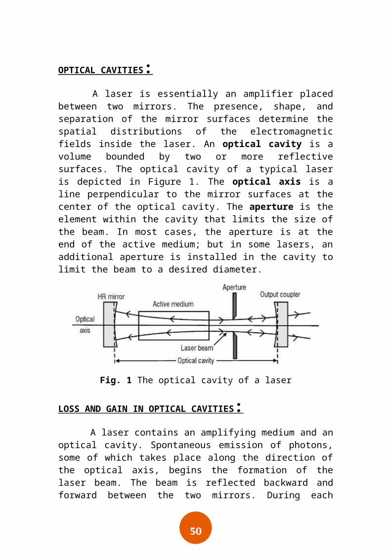
OPTICAL CAVITIES : A laser is essentially an amplifier placed between two mirrors. The presence, shape, and separation of the mirror surfaces determine the spatial distributions of the electromagnetic fields inside the laser. An optical cavity is a volume bounded by two or more reflective surfaces. The optical cavity of a typical laser is depicted in Figure 1. The optical axis is a line perpendicular to the mirror surfaces at the center of the optical cavity. The aperture is the element within the cavity that limits the size of the beam. In most cases, the aperture is at the end of the active medium; but in some lasers, an additional aperture is installed in the cavity to limit the beam to a desired diameter.

50

Fig. 1 The optical cavity of a laser

LOSS AND GAIN IN OPTICAL CAVITIES : A laser contains an amplifying medium and an optical cavity. Spontaneous emission of photons, some of which takes place along the direction of the optical axis, begins the formation of the laser beam. The beam is reflected backward and forward between the two mirrors. During each round trip of the cavity, the beam passes through the active medium twice and is amplified; some of the light passes through the output coupler to form the output beam, and some of the light is removed from the beam due to losses in the cavity. The remaining portion of the light energy is reflected back into the optical cavity. All these factors must be considered in the design of a laser optical cavity.

LOSS IN OPTICAL CAVITIES : The following factors contribute to losses within the optical cavities of lasers:

1-Misalignment of the mirrors: If the mirrors of the cavity are not aligned properly with the optical axis, the beam will not be contained within the cavity, but will move farther toward one edge of the cavity after each reflection.

2-Dirty optics: Dust, dirt, fingerprints, and scratches on optical surfaces scatter the laser light and cause permanent damage to the optical surfaces. Instructions for the cleaning of laser optics are presented later in this module.

3-Reflection losses: Whenever light is incident on a transparent surface, some portion of it always is reflected. Brewster windows and antireflection coatings greatly reduce this loss of light but cannot

51

eliminate it entirely.

4-Diffraction loss: Part of the laser light may pass over the edges of the mirror or strike the edges of the aperture and be removed from the beam. This is the largest loss factor in many lasers.

When a light beam passes through a limiting aperture, the waves at the edge of the beam bend outward slightly, causing the beam to diverge. This phenomenon is termed "diffraction." When laser light moves from left to right (Figure 1), diffraction occurs at the aperture, and the beam diverges. When the beam returns to the aperture after reflection from the HR mirror, its diameter is larger than the diameter of the aperture; and the edges of the beam are blocked. The portion of the beam that does pass through the aperture is diffracted again and experiences additional loss on the next pass.

LOOP GAIN : The loop gain of a laser is the ratio of the power of the beam at any point in the cavity to the power at the same point one round trip (loop) earlier through the cavity.

The power of the beam at point 1 in Figure 2 is P1. When the light passes through the active medium at point 2, it is amplified to a power of P2 = GaP1. After reflection from the HR mirror, the power is P3 = R1GaP1. This light passes through the active medium again and is amplified to have a power of P4= GaR1GaP1. After reflection from the output coupler at point 5, the power is P5 = R2GaR1GaP1. This loop accounts for all modifications on the initial beam except for losses. If the round-trip loss is L, the power remaining at point 1 after one complete circuit of the optical cavity is P6 = P5(1-L), or P6 = R2GaRlGaPl(1-L). Point 6 is identical with point 1 and signifies the completion of one loop.

Fig. 2 Loop gain of a laser

52

The loop gain of the laser, then, is the ratio of P6 to Pl, as indicated by Equation 1.

Equation 1

Given: A ruby laser has the following characteristics (refer to Figure 2):

Ga = 3.0R1 = 0.995R2 = 0.50L = 0.08

Find: Loop gain.

Solution: GL = G2R1R2(1 – L)GL = (3.0)2(0.995)(0.50)(1 – 0.08)GL = (9.0)(0.995)(0.50)(0.92)GL = 4.12

Given: The following are characteristics of the components of an argon ion laser:

Reflectivity of HR mirror: 99.8% Transmission of output coupler

(T): 4.2% Scattering and absorption loss of

output coupler (S + A): 0.05% Round-trip loss (excluding

mirror loss): 0.8% Amplifier gain: 1.05

Find: Loop gain.

Solution: Determine reflectivity of output coupler:

53

R2 = 1 – (T + S + A)R2 = 1 – (0.042 + 0.0005)R2 = 1 – (0.0425)R2 = 0.9575

Write remaining quantities as decimal fractions:

R1 = 0.998Ga = 1.05L = 0.008

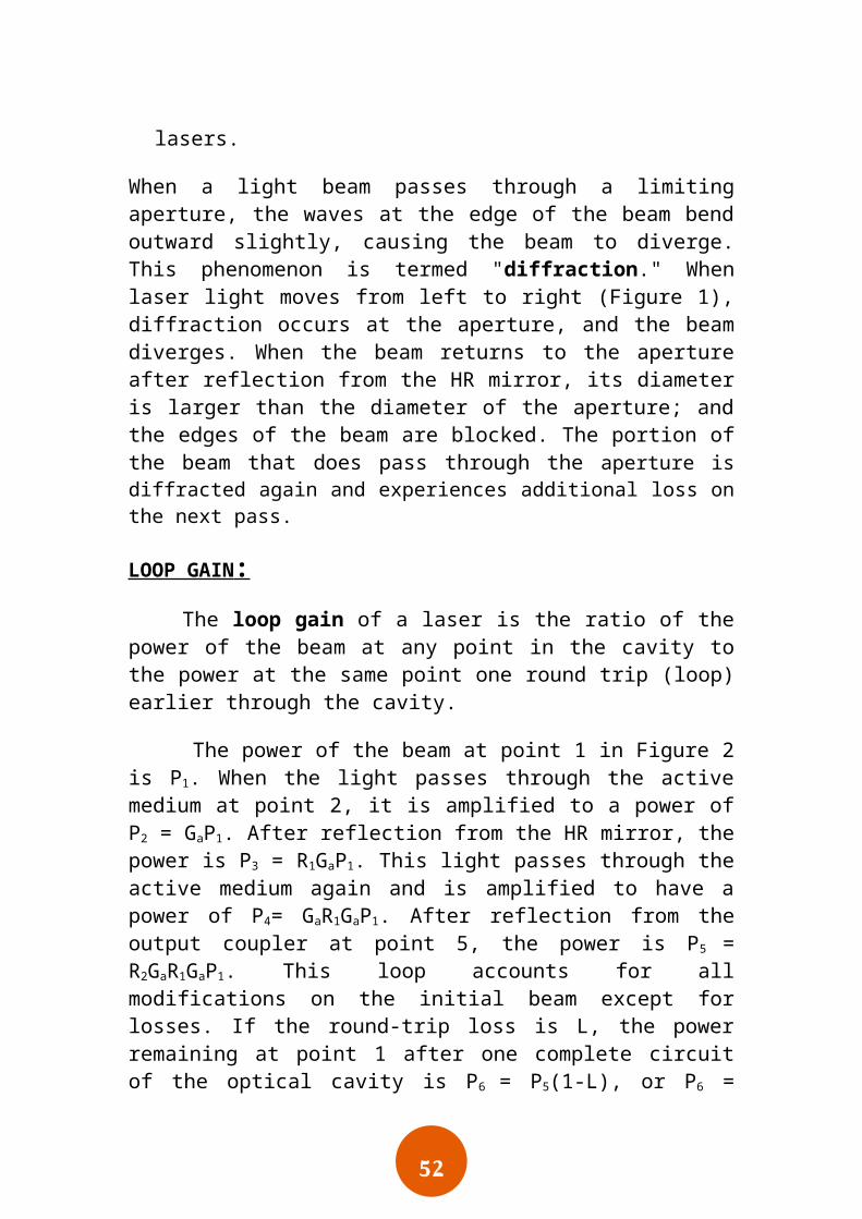
Calculate the loop gain:

GL = Ga2R1R2(1 – L)

GL = (1.05)2(0.998)(0.9575)(1 – 0.008)GL = (1.1025)(0.998)(0.9575)(0.992)GL = 1.045

If the loop gain of a laser is greater than one, the laser output power is increasing. If the loop gain is less than one, the output power is decreasing. If the loop gain is exactly one, the output power is steady.

GAIN IN CW LASERS :

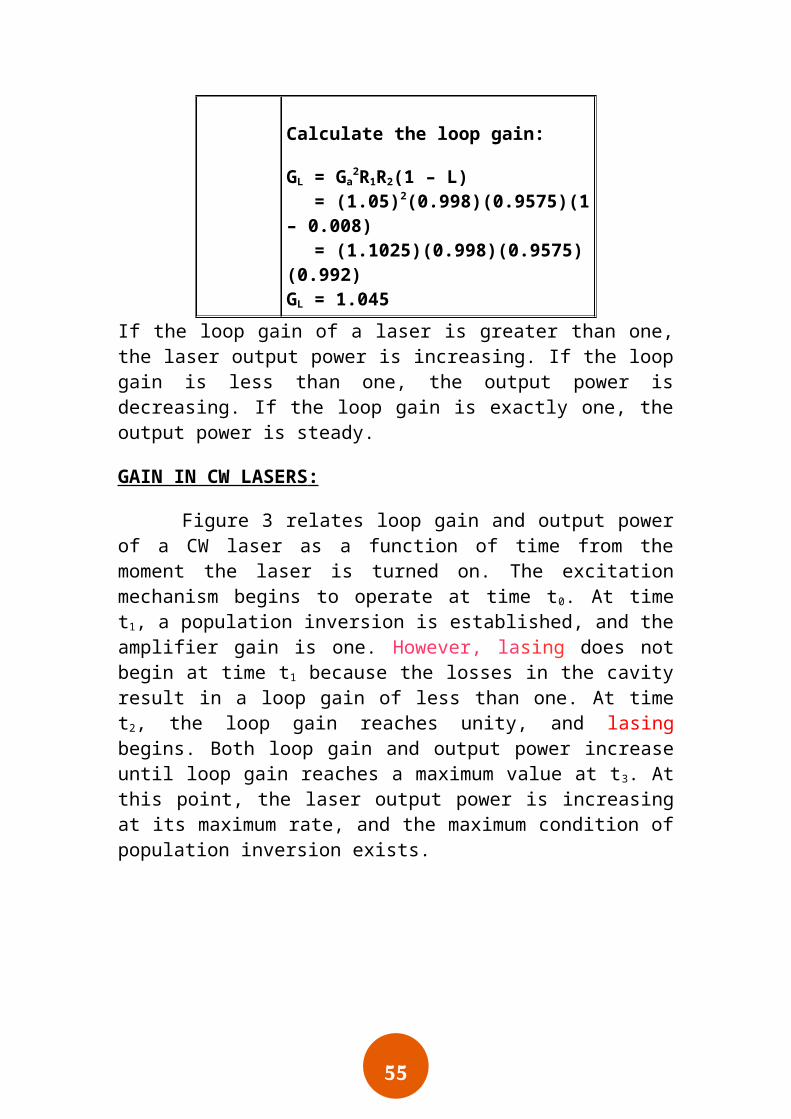
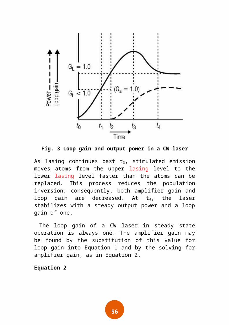
Figure 3 relates loop gain and output power of a CW laser as a function of time from the moment the laser is turned on. The excitation mechanism begins to operate at time t0. At time t1, a population inversion is established, and the amplifier gain is one. However, lasing does not begin at time t1 because the losses in the cavity result in a loop gain of less than one. At time t2, the loop gain reaches unity, and lasing begins. Both loop gain and output power increase until loop gain reaches a maximum value at t3. At this point, the laser output power is increasing at its maximum rate, and the maximum condition of population inversion exists.

54

Fig. 3 Loop gain and output power in a CW laser

As lasing continues past t3, stimulated emission moves atoms from the upper lasing level to the lower lasing level faster than the atoms can be replaced. This process reduces the population inversion; consequently, both amplifier gain and loop gain are decreased. At t4, the laser stabilizes with a steady output power and a loop gain of one.

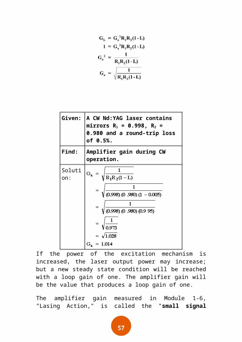
The loop gain of a CW laser in steady state operation is always one. The amplifier gain may be found by the substitution of this value for loop gain into Equation 1 and by the solving for amplifier gain, as in Equation 2.

Equation 2

55

Given: A CW Nd:YAG laser contains mirrors R1 = 0.998, R2 = 0.980 and a round-trip loss of 0.5%.

Find: Amplifier gain during CW operation.

Solution:

If the power of the excitation mechanism is increased, the laser output power may increase; but a new steady state condition will be reached with a loop gain of one. The amplifier gain will be the value that produces a loop gain of one.

The amplifier gain measured in Module 1-6, "Lasing Action," is called the "small signal gain," which is the gain of the active medium for optical signals that are so small that their amplification does not significantly reduce the population inversion. The actual amplifier gain of CW lasers is less than the small signal gain because the power removed by the laser beam does reduce the population inversion. This reduced value of amplifier gain is referred to as "saturated gain."

GAIN IN PULSED LASERS : The instantaneous power of the pulsed laser excitation mechanism far exceeds that of CW lasers. Much greater population inversion and much higher values for both amplifier gain and loop gain are achieved in pulsed lasers. Figure 4 graphically shows the loop gain and output power of a pulsed laser as a function of time. At t1, the loop gain has reached a value of one, and lasing has begun. Loop gain continues to increase to some

56

maximum value at t2, and output rises accordingly.

Fig. 4 Loop gain and output power of a pulsed laser

At t3, the loop gain drops below one, and the power begins to drop. The beam inside the active medium is so intense that it depletes the population inversion entirely by the time lasing stops at t4, from which point loop gain rises again. At t5, loop gain is one again, and lasing begins again. This process is repeated many times during a single pulse of excitation mechanism, resulting in hundreds or thousands of spikes in the output pulse.

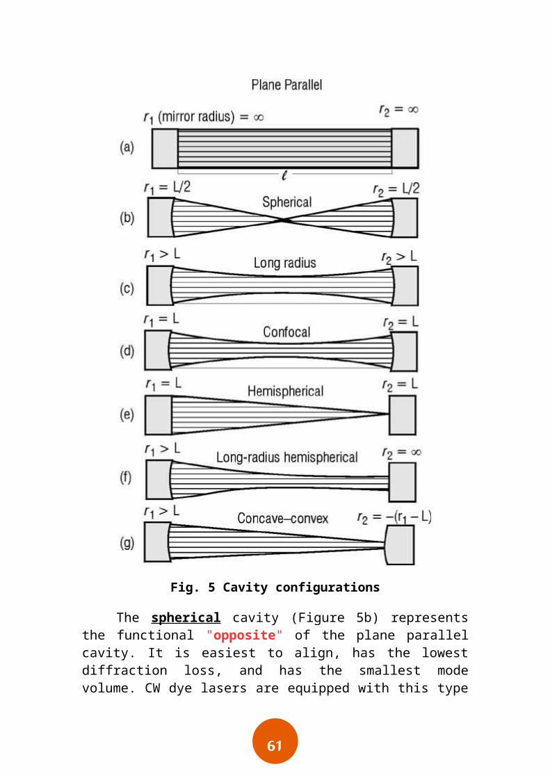
CAVITY CONFIGURATIONS : Figure 5 displays seven cavity configurations commonly used in lasers. In each diagram, the shaded area is referred to as the "mode volume," which is the volume inside the cavity actually occupied by the laser beam. Stimulated emission occurs only within this volume. Parts of the active medium outside this mode volume do not contribute to losing because no beam is present to stimulate the emission of photons. The selection of a cavity configuration for a particular laser depends upon the following

57

three factors:

Diffraction loss. Mode volume. Ease of alignment.

The plane-parallel cavity (Figure 5a) is an important component in pulsed solid lasers and some other pulsed lasers because its high mode volume makes efficient use of the active medium. The cavity has the highest diffraction loss of any configuration, but this loss is overcome easily in pulsed lasers by the additional gain achieved by the larger mode volume. It has the additional advantage of not focusing the laser beam inside the active medium. Such internal focusing can damage solid laser rods. The plane parallel cavity is, however, the most difficult to align, since plane mirrors do not "focus" or concentrate the laser beam within the cavity as do the others. A small tilt of either of the plane parallel mirrors causes the beam to "walk out" of the cavity, thereby frustrating laser action.

58

Fig. 5 Cavity configurations

The spherical cavity (Figure 5b) represents the functional "opposite" of the plane parallel cavity. It is easiest to align, has the lowest diffraction loss, and has the smallest mode volume. CW dye lasers are equipped with this type of cavity because a focused beam is necessary to cause efficient stimulated emission of these lasers. The spherical cavity is not commonly

59

used with any other type of laser.

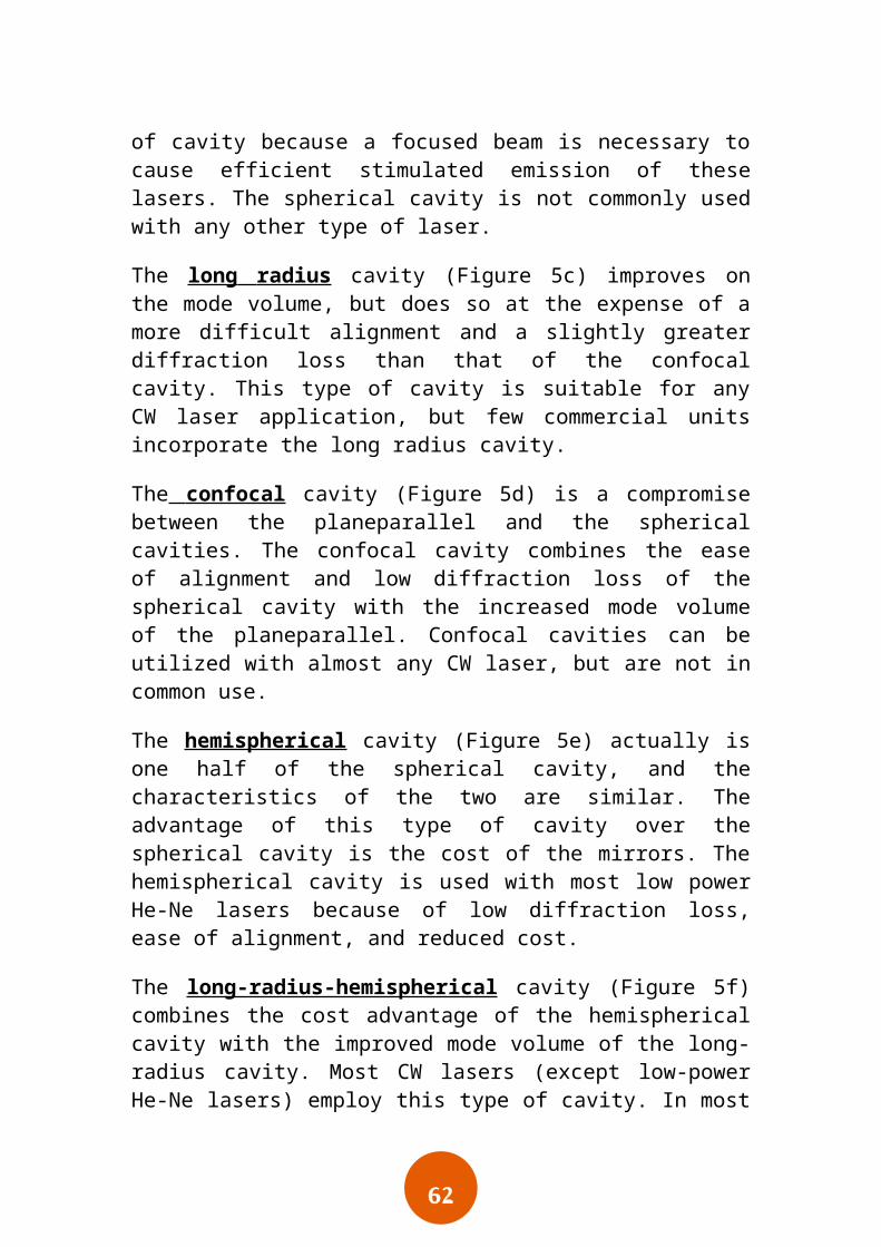
The long radius cavity (Figure 5c) improves on the mode volume, but does so at the expense of a more difficult alignment and a slightly greater diffraction loss than that of the confocal cavity. This type of cavity is suitable for any CW laser application, but few commercial units incorporate the long radius cavity.

The confocal cavity (Figure 5d) is a compromise between the planeparallel and the spherical cavities. The confocal cavity combines the ease of alignment and low diffraction loss of the spherical cavity with the increased mode volume of the planeparallel. Confocal cavities can be utilized with almost any CW laser, but are not in common use.

The hemispherical cavity (Figure 5e) actually is one half of the spherical cavity, and the characteristics of the two are similar. The advantage of this type of cavity over the spherical cavity is the cost of the mirrors. The hemispherical cavity is used with most low power He-Ne lasers because of low diffraction loss, ease of alignment, and reduced cost.

The long-radius-hemispherical cavity (Figure 5f) combines the cost advantage of the hemispherical cavity with the improved mode volume of the long-radius cavity. Most CW lasers (except low-power He-Ne lasers) employ this type of cavity. In most cases, r1 > 2L.

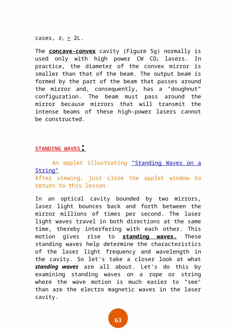
The concave-convex cavity (Figure 5g) normally is used only with high power CW CO2 lasers. In practice, the diameter of the convex mirror is smaller than that of the beam. The output beam is formed by the part of the beam that passes around the mirror and, consequently, has a "doughnut" configuration. The beam must pass around the mirror because mirrors that will transmit the intense beams of these high-power lasers cannot be constructed.

STANDING WAVES : An applet illustrating "Standing Waves on a String"After viewing, just close the applet window to return to this lesson.

In an optical cavity bounded by two mirrors, laser light bounces back and forth between the mirror millions of times per second. The laser light

60

waves travel in both directions at the same time, thereby interfering with each other. This motion gives rise to standing waves. These standing waves help determine the characteristics of the laser light frequency and wavelength in the cavity. So let's take a closer look at what standing waves are all about. Let's do this by examining standing waves on a rope or string where the wave motion is much easier to "see" than are the electro magnetic waves in the laser cavity.

Look at Figure 6. Here we see a rope or string fixed at one end and free to move at the other. If you shake the free end of the rope up and down, you produce "rope waves" that travel to the fixed end and back again to the jiggling end. If you continue to shake the rope in this fashion, quite a jumble of rope motion occurs, since the waves traveling back and forth along the rope interfere with each other. One wave pulls the rope up, another wave pulls it down. However, if you jiggle the rope with exactly the right frequency, the regions where the rope waves add to each other (called constructive interference) and the regions where the rope waves subtract from each other (called destructive interference) occur at the same positions and cause the rope waves to appear to stand still—with a given "profile". This profile is called a "standing" wave.

61

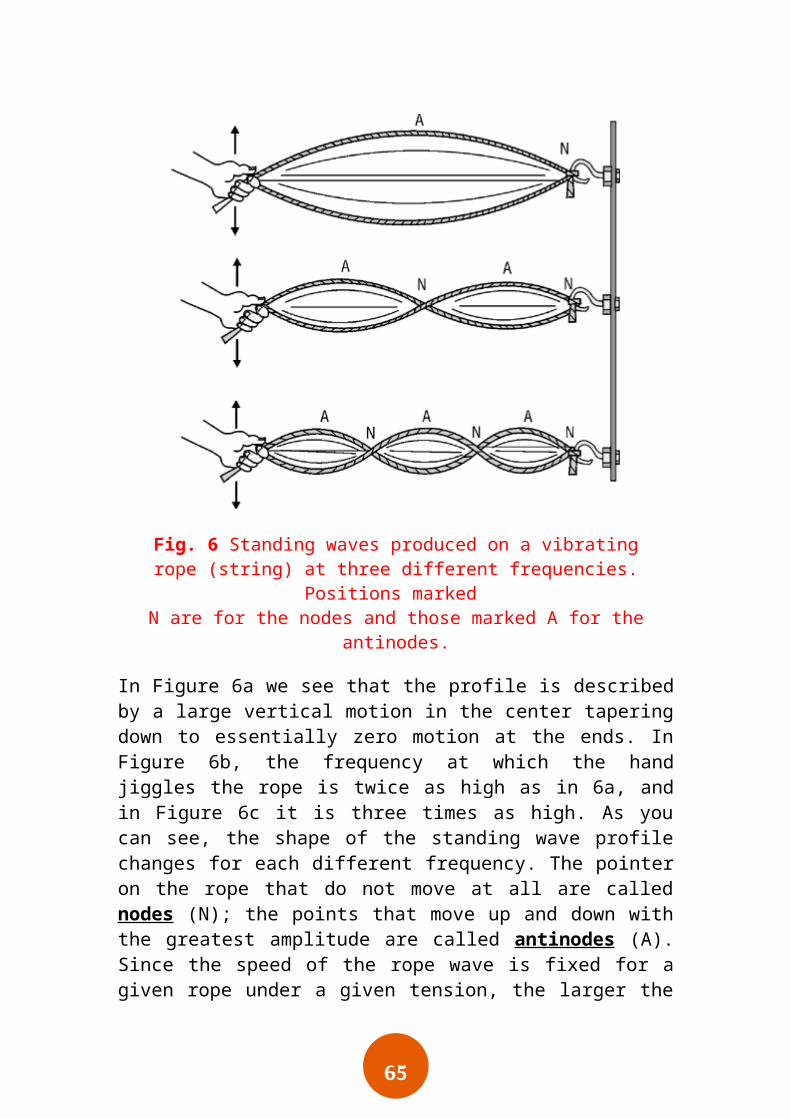
Fig. 6 Standing waves produced on a vibratingrope (string) at three different frequencies. Positions marked

N are for the nodes and those marked A for the antinodes.

In Figure 6a we see that the profile is described by a large vertical motion in the center tapering down to essentially zero motion at the ends. In Figure 6b, the frequency at which the hand jiggles the rope is twice as high as in 6a, and in Figure 6c it is three times as high. As you can see, the shape of the standing wave profile changes for each different frequency. The pointer on the rope that do not move at all are called nodes (N); the points that move up and down with the greatest amplitude are called antinodes (A). Since the speed of the rope wave is fixed for a given rope under a given tension, the larger the frequency of vibration, the smaller the wavelength of the rope waves, in accordance with the relationship –wave speed equals wave frequency times wavelength. Note carefully that it is the overall profile of the wave which appears to stand still. The rope does remain still at the nodes but undergoes a rapid up and down motion between the nodes.

The lowest frequency of vibration which produces a standing wave is called the fundamental–shown in Figure 6a. At whole number multiples of their fundamental frequency, other standing waves are formed, as in Figures 6b and 6c. But at all intermediate frequencies standing waves do not form. When standing waves do form, the frequencies are called resonant frequencies. An important result here is that the distance between successive nodes is equal to half a wavelength of the standing wave. Thus if the distance from hand to rope in Figure 6a is given as L, the wavelength of the wave in 6a is 2L; in Figure 6b it is L, and in Figure 6c it is 2/3L. Knowing the distance L, then, and the number of nodes along L, one can always determine the wavelenth and frequency of the standing wave.

One interesting feature of standing rope waves is that one does not see the interference waves that travel back and forth. Rather one see rope motion that is essentially up and down at the antinodes and still at the nodes. When the rope is vibrated at a resonant frequency, very little effort is required to sustain a large amplitude in the standing wave. When the rope is virated at intermediate frequencies, the interfering waves tend to cancel each other out, the rope motion is rather jumbled, and the amplitude of vibration ???? small along the entire rope. Sound waves in organ pipes follow the same behavior in creating loud tones, giving rise to the fundamental and the higher overtones with which organ players are

62

familiar.

Suppose we now stretch a rope (string) between fixed ends as shown in Figure 7a. If we pluck the string somewhere along its length, only a certain set of frequencies will be found to exist in the vibrating string. As we have seen from Figure 6 and the related discussion, only those frequencies will exist whose associated wavelengths are such that a whole number of half wavelengths fit in the distance L. Since a half wavelength exists between successive nodes, we see that in Figure 7b, in

Figure 7c,   in Figure 7d, and   in Figure 7e.

Fig. 7

Fig. 7b

63

Fig. 7c

Fig. 7d

Fig. 7e

Fig. 7 Resonant frequencies possible whena fixed string is plucked.

64

With the understanding of standing waves in a vibrating string, we can better understand the standing electromagnetic waves (light waves) produced in a laser cavity. There the mirrors are like the fixed ends of the rope (string) and the distance between the mirrors is like the length of the rope between the fixed ends. The amplitude of the electric field will be zero at the mirrors (nodes) just as the string had zero amplitude at the fixed ends (Figure 7). The electric field will be of maximum amplitude at points in between the mirrors–the antinodes. Since the wavelength of light is very small (millionths of a meter) and laser cavities are of the order of centimeters long, many standing waves of different frequencies can "fit in" between the two mirrors. The distance between successive nodes of course will be very small. We shall see how all this works in the next section where we dicuss longitudinal laser modes, that is, those standing waves that can exist in a laser cavity of fixed length.

LONGITUDINAL LASER MODES :

Applet illustrating "Ray Trajectories in an Optical Cavity"After viewing, just close the applet window to return to this lesson.

Applet illustrating "Laser Cavity Stability"After viewing, just close the applet window to return to this lesson.

As we have just seen, each longitudinal mode in an optical cavity is a standing wave. One such standing wave is shown in Figure 8, where the positions of the nodes and antinodes should be evident from our discussions of Figures 6 and 7. Note that the standing wave shown satisfies the condition that nodes are located at each end of the cavity. That is, at the mirror surfaces.

Fig. 8 A possible longitudinal laser mode betweenmirrors separated by a distance l

The wavelength of the light shown in Figure 8 is far out of proportion to the cavity length and the mirror size. We have shown 8 wavelengths and that is far too few for a real laser which emits laser radiation. For an actual case, say

65

for an optical cavity of 20 cm emitting visible laser light at 0.5 micrometers, the number of integer wavelengths between the two mirrors would be

You can see that it would be difficult to draw 400,000 wavelengths in Figure 8, but that's how many would be in a 20 cm laser cavity emitting 0.5 m light.

Now we learned earlier that standing waves between fixed points exist as long as an integral number of half-wavelengths can fit exactly between the mirrors. For the laser described above, that would be 800,000 half-wavelengths. So we can have 800,000 half-wavelengths, or we can have 800,001 or 799,999 and so on. The wavelength difference between these three is very small, as you might guess. Since the wavelength of light is so small, we don't have to lengthen or shorten a mode wavelength by very much to exactly fit in another integral number of half wavelengths. In fact, the difference is so small that more than one longitudinal mode (standing wave) does in fact exist in a laser at the same time. That's because a laser does not emit perfectly monochromatic light so that the wavelength spread is enough to overlap many times the wavelength difference between adjacent longitudinal modes. Let's figure out what this wavelength difference between successive longitudinal modes is.

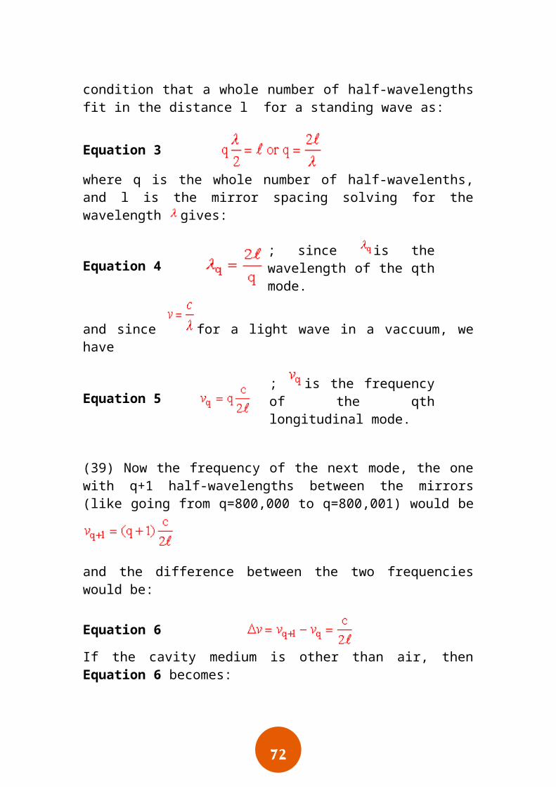
(38) From our work so far we can write out the condition that a whole number of half-wavelengths fit in the distance l  for a standing wave as:

Equation 3

where q is the whole number of half-wavelenths, and l is the mirror spacing solving for the wavelength gives:

Equation 4 ; since is the wavelength of the qth mode.

and since for a light wave in a vaccuum, we have

66

Equation 5 ; is the frequency of the qth longitudinal mode.

(39) Now the frequency of the next mode, the one with q+1 half-wavelengths between the mirrors (like going from q=800,000 to

q=800,001) would be

and the difference between the two frequencies would be:

Equation 6

If the cavity medium is other than air, then Equation 6 becomes:

Equation 7 , where n is the refractive index of the gain medium

So the frequency spacing between longitudinal modes depends only on the spacing between the mirrors (l) and not on the wavelength . For a 20-cm HeNe laser, is equal to

Now the bandwidth of a HeNe laser is much larger than 750 MHz. Remember that the output of a HeNe laser is not exactly 632.8 nm. It has a bandwidth and hence a frequency bandwidth , so that many

langitudinal modes — with spacing can fit within and thus exist simultaneously in the cavity.

Based on Figure 8, Figure 9 shows what two simultaneously oscillating longitudinal modes (standing waves) might look like. (Remember that the wavelengths shown are much, much larger than those for real lasers.)

67

Fig. 9 A diagram of two simultaneously oscillating longitudinal modes in the laser cavity. The shorter

wavelength , mode is described by a frequency vq; the longer wavelenth a lower frequency vq–1.

There are, of course, many more modes possible.

Let's label the one with the shorter wavelength (frequency vq) and the one with a slightly longer wavelength as (frequency vq–1) Necessarily then, vq

mode has a higher frequency than the vq–1 mode. Since the mode numbers of the two differ by one, the vq–1 mode is lower in frequency, by an amount

.

(42) On a gain versus frequency curve for the broadened laser emission— that laser emission amplified by stimulated emission of the laser transition—we can sketch in the longitudinal laser modes. Here we assume tht the vq

mode is at the center of the gain curve. See Figure 10.

68

Fig. 10 Laser gain curve and longitudinal modes.

For the loop gain GL shown, the longitudinal modes, vq, vq–1, vq+1, vq–2 and vq+2

would all be present in the output. The modes vq–3 and vq+3 would not since they fall below GL=1 threshold on the gain curve. Futher, there are no modes possible between the frequencies shown, vq–1, vq+1, etc since these intermediate frequencies do not have wavelengths which fit in the optical cavity of length L. We shall revisit these ideas again when we discuss the spectral distribution of a laser output. But first, let's make some sample calculations to help us understand mode number and mode separation more clearly.

Given: A He-Ne laser (n = 1.0) has a cavity length of 50 cm and an output wavelength of 632.8 nm.

Find: The mode spacing and the longitudinal mode number.

Solution: Mode spacing: (from Equation 7)

Mode number (from Equation 4):

As indicated in Example D, the number of operating modes in most lasers is

69

quite large, as we showed earlier.

In problems that involve gas lasers, the index of refraction usually is considered to be 1.0. However, in solid lasers, the index of refraction of the laser rod must be considered. If mirrors are deposited directly on both ends of the rod, the index of refraction used for mode spacing calculations is the index of refraction of the laser rod. If the cavity also includes a length of air (or other material), Equation 8 is used.

Equation 8

where: n1 = Index of refraction of material one.= Length of material one in meters.

n2 = Index of refraction of material two.= Length of material two in meters.

Given: An Nd:YAG laser has a cavity length of 50 cm and a rod length of 10 cm. The index of refraction of Nd:YAG is 1.823. The remainder of the cavity is filled with air that has an index of 1.0.

Find: Mode spacing.

Solution: n1 = 1.8231 = 0.10

n2 = 1.02 = 0.40

70

SPECTRAL DISTRIBUTION OF LASER OUTPUT:

Figure 11 gives the longitudinal mode pattern of a laser output and the factors that lead to that pattern. In Figure 11a, the broadened laser line relates gain as a function of frequency. The width and height of this curve depend upon the type of active medium, its temperature, and the magnitude of the population inversion. Each type of laser exhibits its own characteristic gain curve.

71

Fig. 11 Spectral distribution of laser output showingfive longitudinal modes in the optical cavity.

The threshold line represents a loop-gain value of one. The active medium provides sufficient gain for lasing at those frequencies at which the loop gain is above the threshold (indicated by the shaded area under the curve). The number of modes that will have a gain of one is dependent on the cavity losses. Cavity losses are a function of optical distortion, surface flaws, transmission (purposeful) through the output coupler and limiting size of aperture.

The rate at which stimulated emission occurs depends, in part, upon the strength of the stimulating signal. Strong optical signals are built up in the laser cavity only at the frequencies that form standing waves. Thus, the only frequencies at which lasing occurs are those frequencies corresponding to the cavity modes. The laser output depicted in Figure 11b consists of five coaxial beams, each with a different frequency and power.

Example F illustrates the wavelength difference between two adjacent modes in a He-Ne laser.

Given: A He-Ne laser has a cavity length of 50 cm and, therefore, a mode spacing of 3.0

72

* 108 Hz. The wavelength of mode q (Figure 8b) is exactly 632.8 nm.

Find: The wavelength of mode q–1.

Solution:

The wavelength difference between the two modes is 4 * 10–13 m, or 4 * 10–4 nm.

As indicated by Figure 11b, each laser mode is not a single frequency, but itself is composed of a range of frequencies. The approximate bandwidth of a single mode is given by Equation 9.

Equation 9

bw = (T + L)

where: = Mode spacing.T = Transmission of output coupler.L = Round trip cavity loss.

(44) This equation is applied in the solution of a typical problem in Example G.

EXAMPLE G: BANDWIDTH OF A LASER MODE

73

Given: A He-Ne laser has a mode spacing of 3.0 * 108 Hz and an output coupler with a transmission of 1.8%. The round-trip loss is 0.4%.

Find: Bandwidth of a single mode.

Solution: bw = (T + L)    = (3 * 108 Hz)(0.018 + 0.004)    = (3 * 108 Hz)(0.022)    = 6.6 * 106 Hzbw = 6.6 MHz

The "fluorescent line width" of a laser is the width of the frequency range over which the spontaneous fluorescence from the upper laser level to the lower laser level occurs. It is always much greater than the line width of the output laser beam. It usually is expressed in frequency units. The fluorescent line width of a typical He-Ne laser is approximately 1.5 GHz. That of a typical Nd:YAG laser is about 30 GHz. The approximate number of modes in a laser output beam can be determined by dividing the laser fluorescent line width by the mode spacing, as indicated by Equation 10.

Equation 10

n =

where: n = Number of modes (an integer).lw = Fluorescent line width of the laser. = Mode spacing.

EXAMPLE H: NUMBER OF MODES IN OUTPUT

Given: The Nd:YAG laser from Example E has a mode spacing of 257.6 MHz The laser fluorescent line width of Nd:YAG is 30 GHz.

Find: The approximate number of modes in the laser output.

74

Solution: