Embed Size (px)
Citation preview

© The McGraw-Hill Companies, Inc., 1999 12.1Irwin/McGraw-Hill
Chapter Outline
12.1 Risk Identification and Evaluation
Identifying Exposures
Property Loss Exposures
Liability Losses
Losses to Human Capital
Losses from External Economic Forces
Evaluating the Frequency And Severity of Loss
Frequency
Severity
Expected Loss and Standard Deviation
© The McGraw-Hill Companies, Inc., 1999 12.2Irwin/McGraw-Hill
Chapter Outline
12.2 Retention and Insurance Revisited
Benefits of Increased Retention
Savings on Premium Loadings
Reducing Exposure to Insurance Market Volatility
Reducing Moral Hazard
Avoiding High Premiums Caused by Asymmetric Information
Avoiding Implicit Taxes due to Insurance Price Regulation
Maintaining Use of Funds
Costs of Increased Retention
Closely-held vs. Publicly-Traded Firms with Widely Held Stock
Firm Size and Correlation Among Losses
Correlation of Losses with Other Cash Flows and with
Investment Opportunities
Financial Leverage
A Basic Guideline for Optimal Retention

© The McGraw-Hill Companies, Inc., 1999 12.3Irwin/McGraw-Hill
Chapter Outline
12.3 Benefits and Costs of Loss Control
Basic Cost-Benefit Tradeoff
Examples of Identifying Benefits and Costs
Installation of Automatic Sprinkler System
Installation of Safety Guards
Child-Resistant Packaging of Non-Prescription Drugs
Qualitative vs. Quantitative Decision-Making
12.4 Statistical Analysis in Risk Management
Approximating Loss Distributions with the Normal Distribution
Illustration
Problems and Limitation
Computer Simulation of Loss Distributions
Illustration
Comparison of Results to Assuming the Normal Distribution
Limitations of Computer Simulation

© The McGraw-Hill Companies, Inc., 1999 12.4Irwin/McGraw-Hill
Chapter Outline
12.5 Use of Discounted Cash Flow Analysis
The Net Present Value Criterion
Example: Forming a Captive Insurer
The Appropriate Cost of Capital
12.6 Summary

© The McGraw-Hill Companies, Inc., 1999 12.5Irwin/McGraw-Hill
Identifying Exposures
● Types of Exposures
• Property• Liability
• Human resource
• External economic factors (e.g., price changes)
● Methods of identification
• Lists
• Understanding business

© The McGraw-Hill Companies, Inc., 1999 12.6Irwin/McGraw-Hill
Assessing Loss Exposures
• Ideally, a risk manager would have information about the probability distribution of losses
• Then assess how different risk management approaches would change the distribution
• Summary measures of probability distributions:
• frequency• severity• expected loss• standard deviation
© The McGraw-Hill Companies, Inc., 1999 12.7Irwin/McGraw-Hill
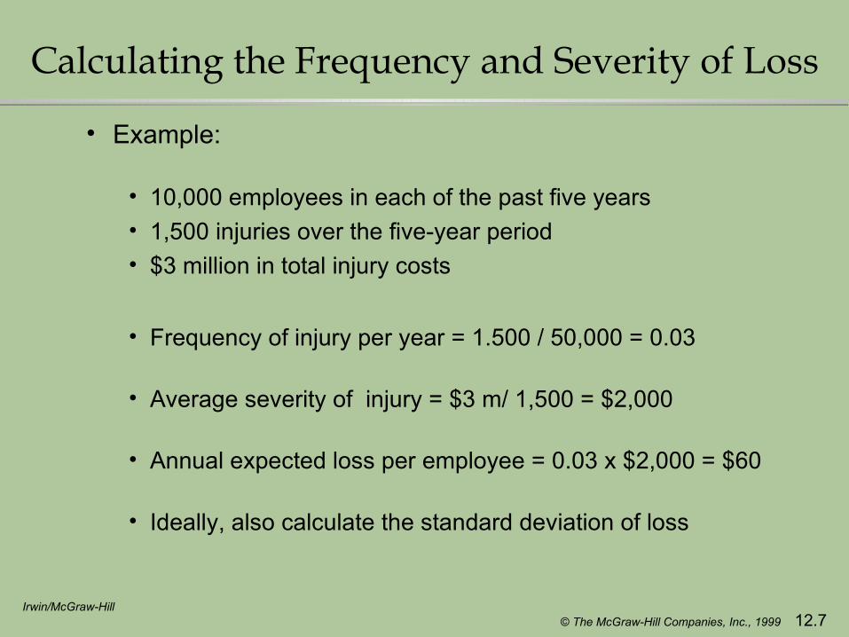
Calculating the Frequency and Severity of Loss
• Example:
• 10,000 employees in each of the past five years
• 1,500 injuries over the five-year period
• $3 million in total injury costs
• Frequency of injury per year = 1.500 / 50,000 = 0.03
• Average severity of injury = $3 m/ 1,500 = $2,000
• Annual expected loss per employee = 0.03 x $2,000 = $60
• Ideally, also calculate the standard deviation of loss
© The McGraw-Hill Companies, Inc., 1999 12.8Irwin/McGraw-Hill
Benefits of Increased Retention
• Savings on insurance premium loadings
• Administrative costs
• Reducing moral hazard
• Avoid being pooled with higher risk policyholders
• Avoid implicit taxes from insurance regulation
• Reducing exposure to insurance market volatility
• Allows firm to maintain use of funds• Questionable
© The McGraw-Hill Companies, Inc., 1999 12.9Irwin/McGraw-Hill
Costs of Increased Retention
• Increased probability of financial distress
• Bankruptcy is costly
• Possibility of distress affects contractual terms with other claimants
• Increased probability of raising external capital
• Forego tax benefits
• Forego efficiencies in bundling services

© The McGraw-Hill Companies, Inc., 1999 12.10Irwin/McGraw-Hill
Factors Affecting Costs of Increased Retention
• Ownership structure (closely-held vs. widely-held firms)
• Firm size
• Correlation among losses
• Correlation of losses with other cash flows
• Correlation of losses with investment opportunities
• Financial leverage
© The McGraw-Hill Companies, Inc., 1999 12.11Irwin/McGraw-Hill
Basic Guideline for Optimal Retention
● Retain reasonably predictable losses and insure potentially large disruptive losses
• Not always right (BP case)
• But often is

© The McGraw-Hill Companies, Inc., 1999 12.12Irwin/McGraw-Hill
British Petroleum Case
● British Petroleum
• Perspective
• risk management strategy• 1990
• Basic Businesses
• Exploration• Oil Refining, Distribution, and Retailing• Chemicals (small)• Nutrition (small)

© The McGraw-Hill Companies, Inc., 1999 12.13Irwin/McGraw-Hill
British Petroleum Case
● Financial Data
• Capital Structure
• Equity = $35 billion • Debt = $15 billion
• After-tax profit
• average = $1.9 billion• standard deviation = $1.1 billion
• Assets
• Diversified: 13,000 service stations in 50 countries • Undiversified: oil production
© The McGraw-Hill Companies, Inc., 1999 12.14Irwin/McGraw-Hill
British Petroleum Case
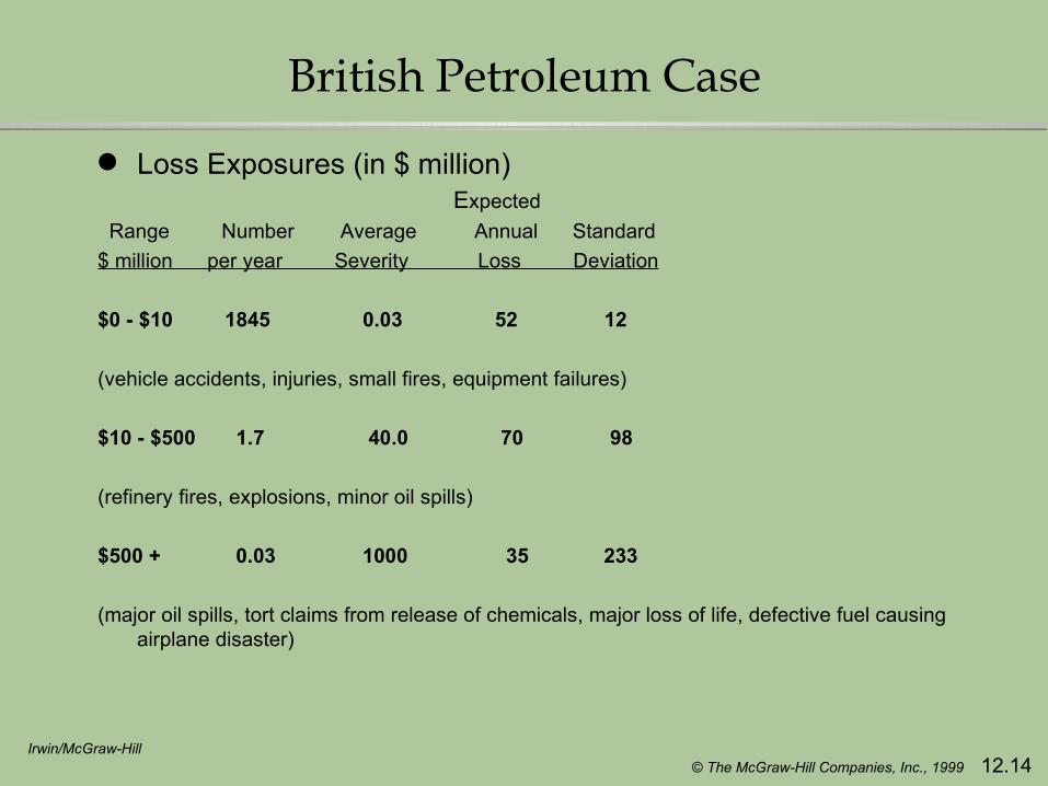
● Loss Exposures (in $ million) Expected
Range Number Average Annual Standard
$ million per year Severity Loss Deviation
$0 - $10 1845 0.03 52 12
(vehicle accidents, injuries, small fires, equipment failures)
$10 - $500 1.7 40.0 70 98
(refinery fires, explosions, minor oil spills)
$500 + 0.03 1000 35 233
(major oil spills, tort claims from release of chemicals, major loss of life, defective fuel causing airplane disaster)
© The McGraw-Hill Companies, Inc., 1999 12.15Irwin/McGraw-Hill
British Petroleum Case
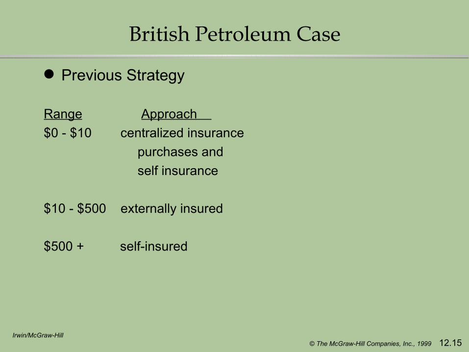
● Previous Strategy
Range Approach
$0 - $10 centralized insurance
purchases and
self insurance
$10 - $500 externally insured
$500 + self-insured

© The McGraw-Hill Companies, Inc., 1999 12.16Irwin/McGraw-Hill
British Petroleum Case
● Conclusions for First Range of Exposures
• Decentralize insurance decisions
• More insurance (Why?)
• local insurers are more efficient in • loss control
• claims processing
• insurance markets are competitive
• insurer insolvency not a concern
© The McGraw-Hill Companies, Inc., 1999 12.17Irwin/McGraw-Hill
British Petroleum Case
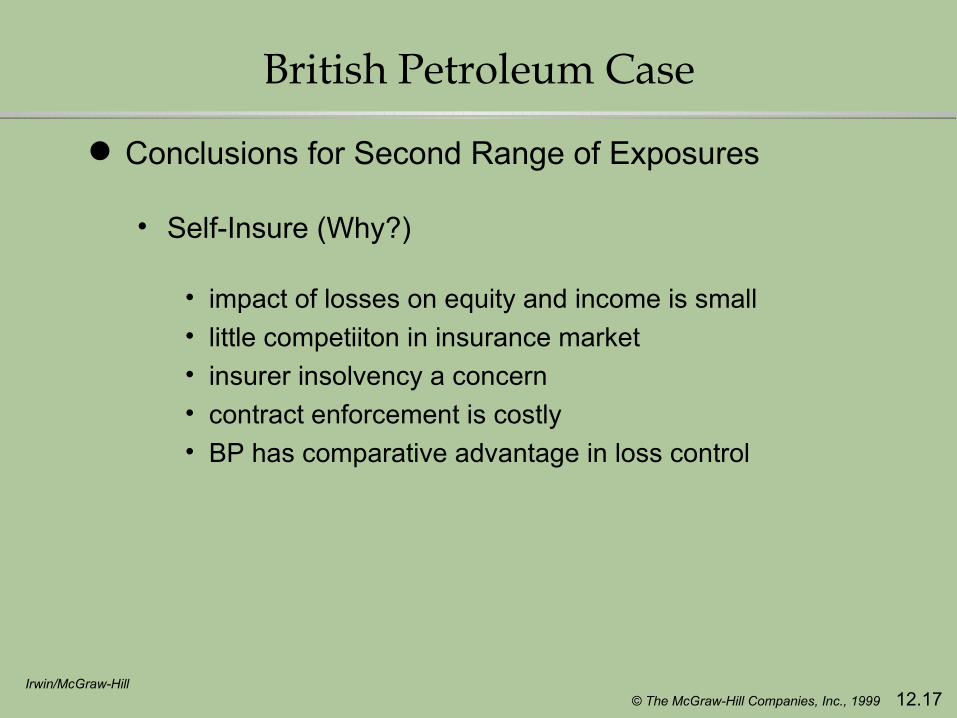
● Conclusions for Second Range of Exposures
• Self-Insure (Why?)
• impact of losses on equity and income is small• little competiiton in insurance market• insurer insolvency a concern• contract enforcement is costly• BP has comparative advantage in loss control

© The McGraw-Hill Companies, Inc., 1999 12.18Irwin/McGraw-Hill
British Petroleum Case
● Conclusions for Third Range of Exposures
• Continue to Self-Insure
• insurance is not availability (not credible)

© The McGraw-Hill Companies, Inc., 1999 12.19Irwin/McGraw-Hill
Making Loss Control Decisions
● Ideally, calculate the present value of the benefits and costs of loss control
• Primary benefit = reduction in expected loss
• Primary costs = cost of loss control device
● Other harder to quantify effects of loss control:
• Lost productivity• Improved contractual terms with employees, etc.
● Quantitative versus qualitative decision making
© The McGraw-Hill Companies, Inc., 1999 12.20Irwin/McGraw-Hill
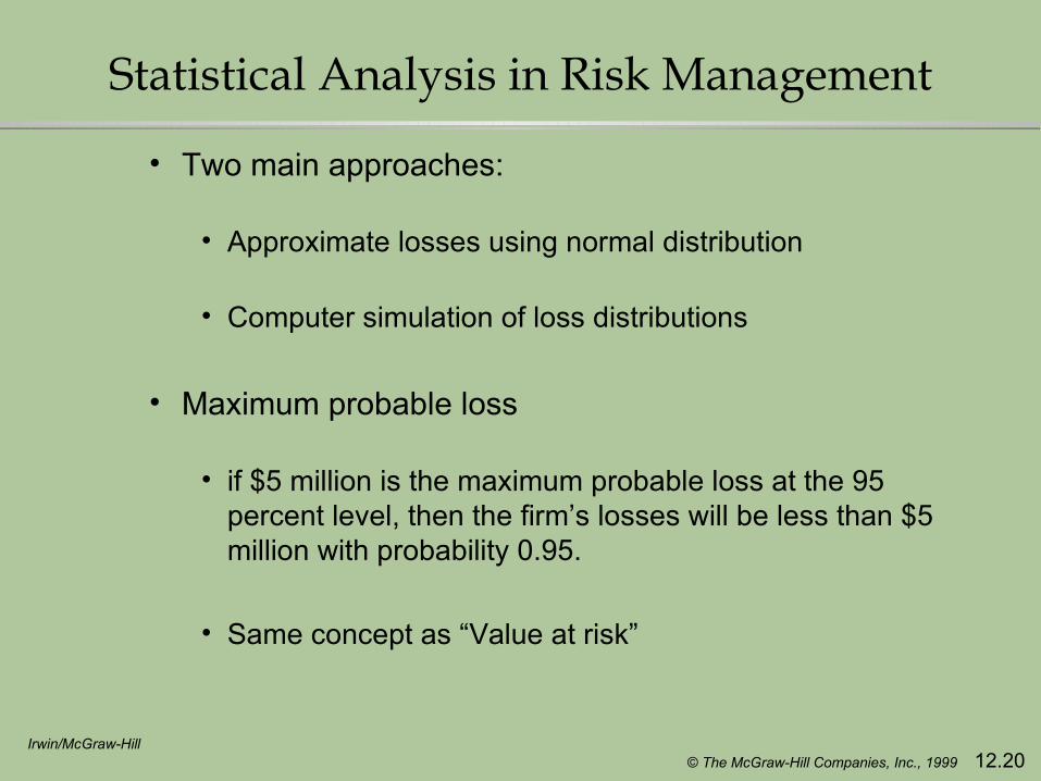
Statistical Analysis in Risk Management
• Two main approaches:
• Approximate losses using normal distribution
• Computer simulation of loss distributions
• Maximum probable loss
• if $5 million is the maximum probable loss at the 95 percent level, then the firm’s losses will be less than $5 million with probability 0.95.
• Same concept as “Value at risk”
© The McGraw-Hill Companies, Inc., 1999 12.21Irwin/McGraw-Hill
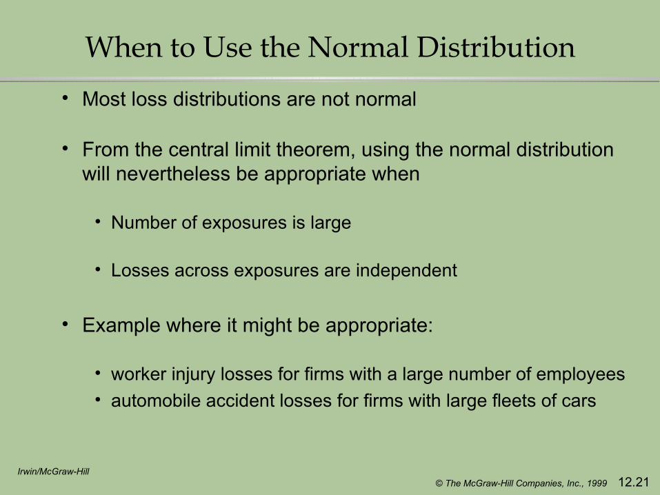
When to Use the Normal Distribution
• Most loss distributions are not normal
• From the central limit theorem, using the normal distribution will nevertheless be appropriate when
• Number of exposures is large
• Losses across exposures are independent
• Example where it might be appropriate:
• worker injury losses for firms with a large number of employees• automobile accident losses for firms with large fleets of cars

© The McGraw-Hill Companies, Inc., 1999 12.22Irwin/McGraw-Hill
Using the Normal Distribution
● Important property
• If Losses are normally distributed with
• mean = m • standard deviation = s
• Then
• Probability (Loss < m + 1.645 s) = 0.95
• Probability (Loss < m + 2.33 s) = 0.99

© The McGraw-Hill Companies, Inc., 1999 12.23Irwin/McGraw-Hill
Using the Normal Distribution - An Example
• Worker compensation losses for Stallone Steel
• sample mean loss per worker = $300
• sample standard deviation per worker = $20,000
• number of workers = 10,000
• Assume total losses are normally distributed with• mean = $3 million
• standard deviation = 100 x $20,000 = $2million
• Then maximum probable loss at the 95 percent level is
• $3 million + 1.645 ($2 million) = $6.3 million

© The McGraw-Hill Companies, Inc., 1999 12.24Irwin/McGraw-Hill
A Limitation of the Normal Distribution
● Applies only to aggregate losses, not individual losses
● Thus, it cannot be used to analyze decisions about per occurrence deductibles and limits
© The McGraw-Hill Companies, Inc., 1999 12.25Irwin/McGraw-Hill
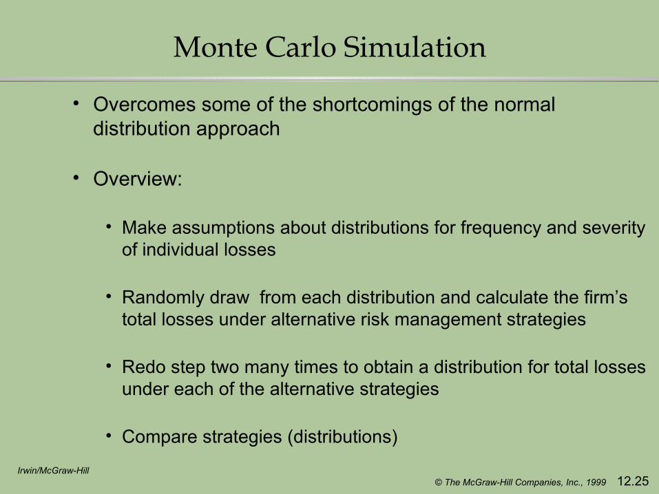
Monte Carlo Simulation
• Overcomes some of the shortcomings of the normal distribution approach
• Overview:
• Make assumptions about distributions for frequency and severity of individual losses
• Randomly draw from each distribution and calculate the firm’s total losses under alternative risk management strategies
• Redo step two many times to obtain a distribution for total losses under each of the alternative strategies
• Compare strategies (distributions)
© The McGraw-Hill Companies, Inc., 1999 12.26Irwin/McGraw-Hill
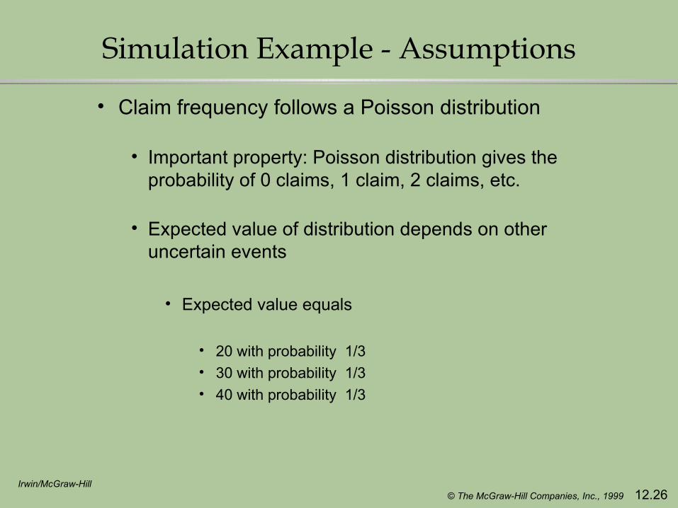
Simulation Example - Assumptions
• Claim frequency follows a Poisson distribution
• Important property: Poisson distribution gives the probability of 0 claims, 1 claim, 2 claims, etc.
• Expected value of distribution depends on other uncertain events
• Expected value equals
• 20 with probability 1/3• 30 with probability 1/3• 40 with probability 1/3

© The McGraw-Hill Companies, Inc., 1999 12.27Irwin/McGraw-Hill
Simulation Example - Assumptions
• Claim severity follows a Lognormal distribution with
• expected value = $100,000
• standard deviation = $300,00
• note skewness

© The McGraw-Hill Companies, Inc., 1999 12.28Irwin/McGraw-Hill
Simulation Example - Assumptions Frequency Distribution with Expected Value
Equal to 30
0
0.05
0.1
0.15
0.2
0.25
0 6
12
18
24
30
36
42
48
54
Number of Claims
PR
OB
AB
ILIT
Y Sample Frequency Distribution with Uncertain
Expected Value (1000 trials)
0
0.05
0.1
0.15
0.2
0.25
0 6
12
18
24
30
36
42
48
54
Number of Claims
PR
OB
AB
ILIT
Y
Sample Loss Severity Distribution(1000 trials)
0
0.02
0.04
0.06
0.08
0.1
0.12
0.0075 0.6 1.2 1.8 2.4 3
Loss in Millions
PR
OB
AB
ILIT
Y

© The McGraw-Hill Companies, Inc., 1999 12.29Irwin/McGraw-Hill
Simulation Example - Alternative Strategies
Policy 1 2 3
Per Occurrence Deductible $500,000 $1,000,000 none
Per Occurrence Policy Limit $5,000,000 $5,000,000 none
Aggregate Deductible none none $6,000,000
Aggregate Policy Limit none none $10,000,000
Premium $780,000 $415,000 $165,000

© The McGraw-Hill Companies, Inc., 1999 12.30Irwin/McGraw-Hill
Simulation Example - Results
No Insurance
0
0.02
0.04
0.06
0.08
0.1
0.12
0.14
0.16
0.18
0.20 1. 5 3 4. 5 6 7. 5 9 10 .5 12
13 .5
Values in Millions
PR
OB
AB
ILIT
Y $500,000 per Occurrence Retention
0
0.02
0.04
0.06
0.08
0.1
0.12
0.14
0.16
0.18
0.2
0 1. 5 3 4. 5 6 7. 5 9 10 .5 12
13 .5
Values in Millions
PR
OB
AB
ILIT
Y
$6 Million Aggregate Annual Retention
0
0.02
0.04
0.06
0.08
0.1
0.12
0.14
0.16
0.18
0.2
0 1. 5 3 4. 5 6 7. 5 9 10 .5 12
13 .5
Values in Millions
PR
OB
AB
ILIT
Y
$1 Million per Occurrence Retention
0
0.02
0.04
0.06
0.08
0.1
0.12
0.14
0.16
0.18
0.2
0 1. 5 3 4. 5 6 7. 5 9 10 .5 12
13 .5
Values in Millions
PR
OB
AB
ILIT
Y

© The McGraw-Hill Companies, Inc., 1999 12.31Irwin/McGraw-Hill
Simulation Example - Results
Statistic Policy 1: Policy 2: Policy 3: No insurance
Mean value of retained losses $2,414 $2,716 $2,925 $3,042
Standard deviation of retained losses 1,065 1,293 1,494 1,839
Maximum probable retained loss at 95% level 4,254 5,003 6,000 6,462
Maximum value of retained losses 11,325 12,125 7,899 18,898
Probability that losses exceed policy limits 1.1% 0.7% 0.1% n.a.
Probability that retained losses ≤ $6 million 99.7% 98.7% 99.9% 92.7%
Premium $780 $415 $165 $0
Mean total cost 3,194 3,131 3,090 3,042
Maximum probable total cost at 95% level 5,034 5,418 6,165 6,462

© The McGraw-Hill Companies, Inc., 1999 12.32Irwin/McGraw-Hill
Discounted Cash Flow (DCF) Analysis
• When risk management decisions affect cash flows over multiple periods, the effect on value should be calculated using DCF analysis
• Calculate the Net Present Value (NPV) of the alternative decisions
• NPV =
• where • NCFt == net cash flow in year t
• r = opportunity cost of capital (reflects the risk of the cash flows)
∑+=
n
0ttt
)r1(
)NCF(E