Rushing to Overpay: Modeling and Measuring the REIT Premium

S. Nuray Akin

Assistant Professor of Economics Economics Department

University of Miami sakin@bus.miami.edu

Val E. Lambson

Professor of Economics Economics Department

Brigham Young University val_lambson@byu.edu

Grant R. McQueen

William Edwards Professor of Finance Marriott School

Brigham Young University mcqueen@byu.edu

Brennan Platt

Assistant Professor of Economics Economics Department

Brigham Young University brennan_platt@byu.edu

Barrett A. Slade*

Professor of Finance Marriott School

Brigham Young University bslade@byu.edu

Justin Wood

Finance Department University of Iowa

justin-wood@uiowa.edu JEL classification: R33, R32, D83 Key Words: Real Estate Investment Trusts (REITs), equilibrium search, hedonic price analysis, repeat-sales analysis, market efficiency, deadlines *Communicating author: Barrett Slade, 692 TNRB, Marriott School, Brigham Young University, Provo, UT 84602. Tel: (801) 422-3504. The authors thank Troy Carpenter and Greg Adams for programing support and Chris Parmeter and participants at BYU, the University of Utah, and the AREUEA 2011 Midyear Meetings for helpful comments. This work was partially supported by the William Edwards professorship, the J. Cyrll Johnson Fellowship, and the Harold R. Silver Fund at BYU.

Rushing to Overpay: Modeling and Measuring the REIT Premium

Abstract

We explore the questions of why Real Estate Investment Trusts (REITs) pay more for real estate than non-REIT buyers and by how much. First, we develop a search model where REITs optimally pay more for property because (1) they are willing, due to cost of capital advantages and, (2) they are occasionally rushed, due to external regulatory time constraints and internal incentives to deploy capital. Second, we test the model using a repeat-sales methodology that controls for unobserved property characteristics, and derive more plausible estimates of the REIT premium. Consistent with our model, we also find the REIT-buyer premium depends on the size of the REIT advantage, the rush to deploy, and the relative presence of REITs in the market.

1. Introduction

Prior research (Hardin and Wolverton (1999), Lambson, McQueen, and Slade (2004), and Ling and

Petrova (2009)) documents that Real Estate Investment Trusts (REITs) pay more for commercial

properties than non-REITs, but the estimated size of the premium is implausibly high. We contribute to

the pricing and real estate literature both theoretically and empirically. Theoretically, we develop an

equilibrium model exhibiting a higher average price for REIT buyers under specific conditions similar to

those in the real estate market. Empirically, we test the model using repeat sales to control for

unobservables and document that REITs, on average, pay a 6.4% premium for commercial real estate.

Our theoretical contribution speaks to a prior, largely informal, literature that posits various

explanations for the REIT premium. For example, Linneman (1997) and Hardin and Wolverton (1999)

appeal to economies of scale, Graff and Webb (1997) and Hardin and Wolverton (1999), to supply

constraints, Graff (2001), to deployment deadlines, and Lambson, McQueen, and Slade (2004) to search

costs and price anchoring. We develop a sequential search model of real estate pricing with two types of

buyers: REITs and non-REITs. REIT buyers have: a) tax or capital-access advantages relative to non-

REITs, and b) external (regulatory) and internal (incentives) pressure to deploy the capital quickly. The

sellers in our model maximize profits by choosing either a high or a low price. The low price is acceptable

to any buyer. The high price is only accepted by REITs who must make a timely purchase to retain the

2

benefits of being a REIT. In equilibrium, asking either price is equally profitable to a seller since fewer

buyers are willing to pay the high price, and hence the transaction is less likely to occur. Thus, in our

model, REITs pay a premium on average.

Equilibrium search theory has identified several environments where multiple prices endogenously

arise in equilibrium. These models rely on buyer heterogeneity in search costs (e.g., Salop and Stiglitz

(1976), Wide and Schwartz (1979), and Rob (1985)), valuations (Diamond (1987)), or number of

simultaneous searches (Burdett and Judd (1983)). Our model is the first to generate price dispersion due to

a benefit that is contingent on completing a purchase before a deadline.1

Although our theoretical model is constructed and applied in a real estate setting, it extends to other

markets where extra benefits can be obtained (or penalties avoided) if a transaction is completed in a hurry.

For example, private equity funds may have fewer government regulations, exchange requirements, and

agency problems than the publicly-traded companies bidding against them. Fund managers are typically in

a hurry to deploy their capital and start earning the management fee. Rushed managers may optimally pay

a premium for an acquisition target. Likewise, a non-profit organization has a clear tax advantage; yet, to

maintain its tax-exempt status under IRS Code Section 501(c)(3), it must spend a stipulated portion of its

endowment assets or endowment investment income. For example, at year end of 2009, the Getty

Museum endowment was $4.9 billion and the museum needed to spend 4.25% ($208 million) during the

year or risk its tax exemption. Spending $208 million on art in one year could be difficult given that

amount is larger than most museums’ total endowment. Our model suggests that the museum may

optimally pay a premium for art when the deadline is looming.2

Our first empirical contribution speaks to a prior literature including Hardin and Wolverton (1999),

Lambson, McQueen and Slade (2004), and Ling and Petrova (2009) that generated seemingly implausible

REIT premiums. For example, Lambson, McQueen and Slade (2004, p. 110) use a hedonic model that

1 Search in the presence of deadlines is also a feature of labor market models where unemployment benefits are withdrawn after a deadline. See Akin and Platt (2011) for a survey of the labor market findings. 2 In 2010 the Getty Museum beat five other bidders to buy Turner’s “Modern Rome—Campo Vaccino” for nearly $50 million, setting a record for the British artist’s paintings.

3

finds, “for REITs, the overpayment is substantial; 31.52% on average…” Using commercial real estate

transactions, we find that the extant hedonic pricing models contain an unobserved explanatory variables

bias leading to inflated estimates of the REIT premium. Much of the apparent REIT price premium arises

because REITs buy premium property—property with amenities unobserved by empirical investigators.3

Using a repeat-sales methodology that controls for unobserved independent variables, we find the REIT-

buyer price premium to be about 6.4%.

Our second empirical contribution confirms the mechanisms that generate the REIT premium in our

theoretical model. Specifically, the premium is influenced by the ability to pay (cost of capital advantages,

as measured by being publicly-held and large), the rush to buy (search-time disadvantages as measured by

the presence of a new security issue whose proceeds are deployed quickly), and the proportion of REIT

buyers in the market. Moreover, our model replicates the observed price dispersion with more plausible

parameterizations than existing models.

The paper is organized as follows: Section 2 develops the theory explaining why REIT buyers may

pay a premium for real estate when they have a cost of capital advantage and time constraints on capital

deployment. Section 3 describes our data, while Section 4 develops the empirical model used to examine

price differentials of properties purchased by REIT and non-REIT buyers. Section 5 presents the empirical

results and Section 6 summarizes the overall findings and conclusions. Appendix A extends the theory to

a continuous-time search environment and Appendix B introduces an alternative empirical methodology.

2. Theory

2.1 REIT Characteristics

REITs are effectively a pass-through entity for tax purposes. They are eligible for a deduction of

dividends paid to shareholders. To qualify as REITs however, firms must meet a number of requirements

as defined by the Internal Revenue Code. Aspects of this code create both a rush to deploy and advantages

3 For example, REITs could buy retail properties with better ingress, apartments with nicer swimming pools, offices with grander views, and industrial properties with higher ceilings. These characteristics are typically not reported in common sources of transaction data.

4

relative to non-REITS.

The IRS code’s REIT asset and income tests can create time pressures. The asset test requires that at

the end of each quarter at least 75% of the REIT’s total assets be represented by real estate, cash, and

Government securities.4 One of the income tests requires that, each quarter, at least 75% of the REIT’s

gross income be derived from real estate including rents, interest from mortgages, and gains from selling

real estate.5 For the deployment of new capital, these requirements are imposed after a “1-year period

beginning on the date the real estate trust receives such capital.”6 Consequently, REITs that raise new

capital have one year to deploy the capital in “real estate assets” or risk disqualification and/or penalties.7

Thus, near the end of a quarter and near the first anniversary of raising funds, REITs may be compelled to

buy real estate quickly.8 In addition to these external pressures, REIT managers have internal incentives to

deploy capital quickly. First, they have a contractual obligation to give investors exposure to a specific

real estate asset class. Second, they can have a compensation-related incentive with fees based on

deployed capital. Third, they have a performance-related incentive because they are typically evaluated

relative to a benchmark and unallocated funds create a “cash drag.”

Using the Securities Data Company (SDC) database, we identify the REITs that issued new debt or

equity in the twelve months preceding the purchase of property in our database. Over half of the

transactions occurred within three months of the new issue as if managers had internal incentives to deploy

quickly. Nevertheless, some transactions occur in the 12th month after a new issue, just beating the

external deadline.

Regarding advantages, REITs have a tax advantage relative to corporations because corporate profits

are taxed twice. However, the majority of our database’s transactions are by individuals, partnerships, or 4 Internal Revenue Code, 856(c)(4) 5 Internal Revenue Code, 856(c)(3) 6 Internal Revenue Code, 856(c)(5)(B) 7 Brandon (1998) and Graff (2001) discuss REIT tax issues. Failure to meet the quarterly asset and income requirements can lead to a loss of REIT status. However, Internal Revenue Code, 856(c)(6) and 856(c)(7) allow for REITs who missed just one quarter to retain their status if the failure is due to “reasonable cause” and the REIT takes corrective action which can include a tax, a penalty, and the selling of “offending” assets. 8 In practice, REIT managers could satisfy the time constraint by parking money in, say, Fanny Mae securities. This strategy has the same internal costs as holding cash.

5

limited liability companies that share the REIT tax advantage. Relative to these competitors, REITs have

superior access to capital because they can issue equity through initial public offerings (IPOs) and

secondary offerings. Furthermore, for public REITs, their tradable shares provide increased liquidity. The

size and scope of REITs may lead to economies of scale and diversification benefits. Any of these

advantages could make a REIT willing to pay more for a given property than a non-REIT; our model does

not hinge on the particular nature of the advantage.

2.2 Theoretical Model

Search theory has previously been applied to the analysis of real estate markets with some success.9

Typically, buyers are modeled as drawing prices from an exogenous distribution, each time deciding

whether to purchase the associated property and leave the market, or to draw again. Sellers’ actions are

not derived from maximizing behavior. In contrast, we explicitly model buyers (REITs and non-REITS)

and sellers as optimizers so that prices are endogenously formed. Thus, the interaction between sellers and

buyers determine the distribution of prices in the market.10

We assume sellers post (i.e., ask for) a specific price, and cannot revise that price on meeting a

particular buyer. In Williams (1995) and Albrecht et al. (2007), for example, price is determined through

bilateral bargaining between the buyer and the seller. In these papers, buyers randomly encounter

properties without knowing anything about their price; Nash bargaining then determines the division of

surplus between the buyer and the seller, and hence the price of the real estate. Our price-posting

environment is arguably a reasonable approximation for the real estate market. While some negotiation

9 Search models include Yavas (1992), Sirmans, Turnbull, and Dombrow (1995), and Lambson, McQueen, and Slade (2004). The last is most closely related to our paper. In contrast to our paper, Lambson, McQueen, and Slade (2004) assume an exogenous price distribution and buyers that differ in their outcomes because some have (permanently) higher search costs and thus a higher reservation price. This disadvantage does not change over time. 10 Although we model buyer and seller behavior, we do not model an endogenous choice to enter the market (as a seller, a REIT, or a non-REIT). Sellers exogenously enter the market, being unable to manage their offered property. REITs have a clear advantage over non-REITs, but the latter are unable to change their status to the former, perhaps due to legal hurdles.

6

occurs relative to the asking price, this is usually over a small fraction of the purchase price.11 Moreover,

our price-posting environment allows sellers to target a particular buyer segment through their asking

prices.12

Buyers

In every period, each buyer searches among available properties. For simplicity, we allow buyers to

consider only one property per round; we relax this assumption in Appendix A and obtain a similar

equilibrium solution. Suppose, as will be demonstrated below, that at most two observed prices arise in

the market: a low price!!! and a high price, !! ≥ !!. Let ! be the endogenous probability of encountering

the lower price during the period, so (1 − !) is the probability of encountering the higher price.

If a non-REIT purchases a property, it leaves the market and, by managing the property, derives a cash

flow with a present value of !, an objective value on which all buyers agree. REIT-managed properties

derive an additional profit, denoted by ! > 0; consequently, REITs value the property at ! + !.13 Any

buyer that does not purchase a property during the period continues to search in the subsequent period.

REITs face an additional constraint: if a REIT does not acquire a property, it loses the advantages and is

subsequently treated like a non-REIT.14 Thus, REITs faced with a deadline may find themselves

compelled to pay more to preserve their status.

Allowing buyers to observe only one property in the period before the deadline simplifies the

exposition but it is not crucial. In Appendix A, we provide a generalization in which buyers encounter

properties according to a Poisson process; there, REITs could encounter multiple properties before the

deadline. The pivotal feature in both environments is that the benefit is only available if a REIT deploys its

11 Horowitz (1992) finds a monotonic (and hence invertible) relationship between asking and purchase prices, suggesting that which is used is immaterial to the analysis. 12 Arnold (1999) shows that in practice, when a seller lists a higher price in the MLS, some buyers will not even bother investigating the property further since it would require significant negotiation to bring the price to an acceptable range. This reduces the likelihood that the seller encounters an interested buyer in a given period. 13 Each buyer’s purchase represents one deployment of new capital. A REIT may hold multiple investments, but we do not need to track these holdings since we do not model any interaction among them. 14 In practice, the consequences can be more severe, including losing REIT status on all properties rather than just the newly-deployed capital. Larger penalties will strengthen the two-price equilibrium presented, creating a wider gap between the prices.

7

capital within a specified period of time.

We formulate the buyer’s decision problem using standard dynamic programming methods. Using

subscripts r and n for REITS and non-REITs, respectively, the expected value of a non-REIT beginning its

search, !!, must satisfy:

!! = !max ! − !! , !"! + 1 − ! max ! − !! , !!"! , (1)

where ! is the discount factor.15

The right side of (1) formalizes the following intuition. If a non-REIT acquires a property at price ! in

the current period, it enjoys a profit of ! − !. If it defers purchase for a period, it will find itself in the

same position at the beginning of the subsequent period as it did at the beginning of the current period and

hence will be worth the same. With discounting, the relevant comparison in the current period is between

! − ! and !!!. A non-REIT is worth max ! − !! ,!"! with probability ! and max ! − !! ,!"! with

probability (1 − !). The resulting unconditional expected value is the right side of (1).

Similarly, let !! denote the value of a REIT beginning its search. It faces the same probability of

encountering high or low prices, but the decision differs in two ways. First, a REIT that purchases a

property at price ! receives an additional benefit, !. Second, if a REIT declines to purchase a property, it

loses its REIT status, receiving a discounted continuation payoff of !"! as though it were a non-REIT.

These adjustments to (1) result in (2):

!! = !max ! + ! − !! , !"! + 1 − ! max ! + ! − !! , !"! . (2)

Sellers

Sellers are aware that two kinds of buyers exist but they are unable to predict which kind of buyer will

encounter their posted asking prices. Sellers thus face a trade-off: a lower price entails a smaller markup, 15 Our model assumes an infinite horizon; the market is expected to exist for infinitely many time periods. The infinite horizon need not be interpreted literally. If a strictly positive probability that the market will function for another period exists, say !! ∈ 0,1 , then the probability can be wrapped into the discount factor, ! ∈ 0,1 , so that !! = !!/(1 + !) where ! ∈ [0,∞) is a rate of time preference.

8

but is more likely to induce a purchase. If the property is not sold, the seller retains it to offer again in the

following period.

If equilibrium exhibits both asking prices, then sellers must be indifferent between them. In other

words, the smaller markup must exactly offset the higher probability of sale so as to generate the same

expected profit. Formally, this indifference condition is:

!! = !!!!! + 1 − ! !!!, (3)

where ! is the probability, derived below, that the property will be sold at the higher price. On the left side

is the revenue from posting the low price because it is acceptable to the entire population of buyers.

Posting this price will guarantee a sale this period. On the right side is the expected revenue from posting

the high price, which is only acceptable to fraction ! of the population, namely, the REITs. A non-REIT

will reject the high price; in this case the associated property cannot be sold until the following period, as

is reflected in the second term.

In addition to satisfying Equation (3), equilibrium asking prices must be at least as profitable as any

others.

Steady State

As is typical in the dynamic general equilibrium literature, we focus on steady-state equilibria. Here,

this means that the stock of REITs, say !!, is the same over time and that the stock of non-REITs, say !!,

also is constant from period to period. All REITs that enter in a given period either make a purchase (and

leave the market) or do not make a purchase (and become non-REITs). Hence, no old REITs are in the

market for property. Consequently, if the same number of REITs, say Nr, enter each period, then their

number will be constant over time, so

!! = !!! . (4)

The determination of the steady-state number of non-REITs is more complicated because it has three

components: yesterday’s non-REITs who declined to purchase and thus continue their search as non-

9

REITs, yesterday’s REITs who declined a purchase and thus continue their search as non-REITs, and

newly entered non-REITs. The three types are associated, respectively, with the three terms on the right

side of:

!! = !! ! 1 − !!" + 1 − ! 1 − !!! + !! ! 1 − !!" + 1 − ! 1 − !!! + !!!, (5)

where !!" is the fraction of type ! buyers that purchase a property listed at price !!. The probability of the

high price being paid is thus:

! = !!!!!!!!!!!

!!!!!. (6)

The numerator indicates the number of buyers who are willing to pay the high price, while the

denominator indicates the total number of buyers.16

Equilibrium

The interaction of buyers and sellers in steady state generates one of two equilibria. In the degenerate

equilibrium, all sellers ask for the low price. In the dispersed equilibrium, both prices are observed; only

REITs pay the higher price, being anxious to make a purchase and maintain their benefits as REITs. In

both equilibria, buyers respond the same way to possible prices. Both kinds of buyers are willing to pay

the low price (!!" = !!" = 1), so sellers asking !! sell for certain. REITs are also willing to pay the high

price (!!! = 1), while non-REITs are not (!!! = 0). Table 1 summarizes the solution for each of the two

equilibria.

Constructing the two-price equilibrium is straightforward. First, consider the equilibrium prices. The

low price !! extracts the full surplus of the non-REITs. If !! > !, the non-REITs would reject all offers,

preferring the continuation value, !! = 0; only the REITs might pay such a price, but these are already

16 We assume that the market for construction is perfectly competitive so that a seller can only obtain new properties at cost !, which is equal to the expected revenue from sale. Under this assumption, tracking the steady-state population of sellers is unnecessary. Since sellers are indifferent about entering the market, we can assume they enter at whatever rate is needed to ensure that every buyer will encounter one seller each period.

10

willing to pay !! > !!. Thus, charging !! > ! would be dominated. On the other hand, charging a price

!! < ! cannot increase the probability of a sale because everyone is willing to pay !. Thus, !! < ! is also

dominated.

Similar logic justifies !! = ! + !. Any higher price will be rejected by everyone (since REITs can

obtain a payoff of 0 by waiting for the next period), and any lower price will reduce realized profit but not

increase the probability of payment (since non-REITs will still reject any !! > !!). Thus, although sellers

have the ability to offer a range of prices, their profits are maximized by offering just two, the most non-

REITs are willing to pay and the most REITs are willing to pay.

Using these buyer strategies, equations (4) and (5) simplify as follows:

!! = !!! , (7)

!! = !! 1 − ! + !!!. (8)

Combining equations (3) and (6) with equilibrium prices, we find:

1 − ! ! = !!

!!!!!! + 1 − ! ! . (9)

This system of three equations (7-9) determines the three unknowns, !!, !!, and ! whose solutions are

reported in Table 1. Since ! is a probability, it must satisfy 0 ≤ ! ≤ 1. This implies that the dispersed

equilibrium can only exist if !!! !! ≤ !!

!!. Intuitively, this two-price equilibrium requires the proportion of

REIT buyers (the right side) to exceed the ratio of payoffs from the two prices (the left side). Otherwise,

offering the high price would not be profitable.

On the other hand, in the degenerate (one-price) equilibrium, one must verify that it would not be more

profitable to offer the higher price. Note that the reservation prices of the buyers are still pinned down as

described above; but in this equilibrium, sellers will earn less expected profit if they hold out for a higher

price that is only acceptable to REITs. Substitution of (6) into (3) reveals that the low price is at least as

11

profitable if and only if !!! !! ≥ !!

!!. Hence, the two equilibria are mutually exclusive and one of them

always exists.

In equilibrium, all REITs retain their status. REITs obviously prefer paying the low price since it

generates a positive net present value. However, REITs are also willing to pay the high price this round

(even though paying the high price has a zero NPV) because it is no worse than the alternative of

continuing search in future periods having lost REIT status. Consequently, in the dispersed equilibrium,

REITs pay more than non-REITs on average because they always pay the low price when offered, as do

the non-REITs, but occasionally are offered and pay the high price, yielding an average price of:

!!"# = !!! + 1 − ! !! = ! + ! 1 − 1 − ! !!!!

. Thus, REITs will appear to overpay relative to non-

REITs by !! − 1 − ! !!!!

percent.

Comparative statics on ! reveal that the fraction of sellers offering the lower price will increase with a

rise in ! or !!, and decreases with a rise in !, !, or !!; all of which are intuitive. Essentially, sellers

become more willing to target REITs (and hence reduce !) as it becomes more likely to encounter a REIT

or the percentage difference between the high and low price increases.

3. Data

To test the REIT-buyer effect on prices of real property, we use CoStar transactions data on 252,729

office, retail, industrial, and apartment properties that occurred from January 1989 through December

2007. The transactions are located in seven southwestern U.S. counties (Maricopa County, AZ; Clark

County, NV; Los Angeles County, CA; Orange County, CA; Riverside County, CA; San Bernardino

County, CA; San Diego County, CA).17

The CoStar data do not indicate whether the buyer or seller is a REIT. However, they provide the

17 CoStar Group, Inc. investigates, records, and sells commercial property transaction data after confirming the details of the transaction with the relevant parties, including the buyer, seller, and broker. We thank CoStar for their generous assistance with the data.

12

buyer and seller name in each transaction. We matched these names to lists of REIT names from the

Center for Research in Security Prices (CRSP), Securities Data Company (SDC), and Mint Global

databases. The REIT-buyer variable is set equal to one for the 471 transactions where the buyer shows up

on one of the three REIT lists, and zero otherwise. For publicly traded REITs, we use the (SDC) to

identify if the REIT buyers raised either debt or equity financing sometime within the 12-month period

leading up to the property transaction.

Table 2 provides descriptive statistics of the dataset.18 Table 2 Panel A reports summary statistics and

a non-parametric test for differences in distributional equality between REIT and non-REIT buyers in the

total sample. We use a distributional equality test, as opposed to the more common equality of means test,

to illustrate that REITs are primarily interested in a subset of property.19 The null hypothesis of distribution

equality is rejected (e.g., REITs typically purchase larger and newer properties.) Consequently, in our base

case, we restrict our sample to properties greater than 20,000 square feet. This restriction drops the non-

REIT observations from 139,056 to 32,835 (76% of observations intentionally discarded) and drops the

REIT-purchased sample from 471 down to 417 (loss of 11%).20

Table 2 Panel B shows descriptive statistics conditioning on size, while Panels C and D report the

same for REIT and non-REITs, respectively. The mean sales price and building area for REIT properties

are $19,113,626 and 186,694 square feet respectively, whereas for non-REIT properties the mean price is

$6,720,914 and mean size is 71,197 square feet. REITs also tend to buy newer properties than non REITs

18 Before analyzing the data, we eliminate transactions with missing or questionable values. Specifically, we drop 12,700 observations with inconsistent building square feet; 21,433 condominium conversions; 7,243 non-conventional CoStar property type labels (flex, healthcare, hospitality, specialty, and sports/entertainment); 67,903 observations that have missing data on critical variables, i.e., sales price, building age, building area, and land area; 202 unusual sales conditions such as property contamination or auction sale; 3,716 observations with questionable price data (price per square foot less than $20 or greater than $2,500), and 5 observations with comments indicating the recorded price pays for more than the recorded property. The remaining dataset contains 139,527 observations. 19 The test computes the integrated squared density difference between the estimated densities/probabilities of two samples having identical variables/data types. We used 999 bootstrap replications for each of the five variables under scrutiny and the bandwidths used for each density are standard rule-of-thumb bandwidths. See Li, Maasoumi, and Racine (2009) for further details. 20 Ling and Petrova (2009) truncate their sample at a sales price of $500,000. In practical terms, our 20,000 square foot conditioning translates into a cut-off price of $405,000. We use building size rather than price because price is our dependent variable. All of our results are slightly stronger if we use all 139,527 observations, rather than just the 33,252 largest properties.

13

(mean of 14.39 years versus 22.90 years).

Table 3 provides the descriptive statistics for the binary variables. REIT buyers are more likely to be

out-of-state and purchase a higher proportion of office properties but a lower proportion of retail properties

relative to non-REITs.

REIT buyers are more likely to be involved in a sale-leaseback or a portfolio sale and approximately

42% of all transactions come from Los Angeles County, whereas about 36% of the REIT-buyer

transactions come from Los Angeles County. About 65% of the REIT transactions occurred from 1993

through 1998, the six years with the highest proportion of REIT-buyer transactions. The distribution for

non-REIT transactions is more evenly distributed across time.

4. Methodologies

4.1 Hedonic Model We begin by estimating the following hedonic model to first confirm the high coefficients on the REIT

dummy variable found in the literature.21 The dependent variable, LnPRICE, is regressed on buyer type,

property characteristic, buyer/seller location, property type, transaction characteristic, location, and market

condition (time) variables. The regression model is represented as follows:

,,7

2

2007

1990,,

6

1,,

4

2,,,6,5

,4,3,2,10,

tij t

tttijj

jtijj

jtijjtiti

tititititi

MKTCONDNGEOLOCATIO

TRANSCHARPROPTYPEEBUYOUTSTATESQBUILDINGAG

EBUILDINGAGLnLANDAREAAREALnBUILDINGREITBUYERLnPRICE

εδφ

λβαα

ααααα

+++

++++

++++=

∑ ∑

∑∑

= =

==

(10)

where,

LnPRICEi,t = natural log of sales price for property i in year t; 21 Hardin and Wolverton (1999) empirically examine acquisition premiums by REITs in Atlanta, Phoenix, and Seattle. They find that REITs paid a statistically significant premium of 21.6% in Atlanta and a premium of 27.5% in Phoenix; however, they find no evidence of a REIT premium in Seattle. Lambson, McQueen and Slade (2004) also find a substantial overpayment for apartment properties by REITs in the Phoenix market and Ling and Petrova (2009) find strong empirical support for a REIT buyer premium in nine large metropolitan areas.

14

REITBUYER = a binary variable =1 if the buyer is a REIT;

LnBUILDINGAREA = the natural log of the building area (square feet); LnLANDAREA = the natural log of the land area (acres); BUILDINGAGE = age of building (years); BUILDINGAGESQ = building age squared; BUYOUTSTATE = a binary variable =1 if the buyer resides out of state; PROPTYPE = our binary variables indicating property types: office, retail, industrial,

and apartments; TRANSCHAR = six binary variables indicating whether the transaction was a sale-

leaseback transaction, bank sale, Resolution Trust Corporation (RTC) sale, part of a portfolio sale, distress sale, or a 1031 Tax-deferred Exchange. Consequently, the λ coefficients measure price relative to standard market arms-length transactions;

GEOLOCATION = seven binary variables indicating geographic location of each transaction;

geographic areas include the following counties: Maricopa, AZ; Clark, NV; Los Angeles, CA; Orange, CA; Riverside, CA; San Bernardino, CA; and San Diego, CA;

MKTCOND = market conditions proxied by annual binary variables from 1989 through

2007.

The dependent variable is specified as the natural logarithm of the sales price for two reasons. First,

this form gives less weight to extremely high values (potential outliers) than an untransformed dependent

variable (de Leeuw, 1993). Second, the sales price is constrained at zero on the left side of the

distribution, but skewed on the right side of the distribution; therefore, the specification is consistent with

the distribution of the sales prices in the sample.

The primary variable of interest is REITBUYER. The theoretical model predicts that the coefficient on

REITBUYER, α1, will be positive if REITs are both willing (e.g., capital access advantages) and rushed

(e.g., internal and external time constraints) to pay a premium. If the coefficient is positive and significant,

then REIT-buyer transactions occur at a premium compared with non-REIT transactions, rejecting the null

hypothesis that REIT status has no impact on the purchase price.

15

The building area is specified as the natural log of building square feet (LnBUILDINGAREA). This

specification allows price to increase with building size, at a decreasing rate, which reflects economies of

scale in construction. We predict a positive coefficient on this variable. Land area is also specified as the

natural log. We predict a positive coefficient on LnLANDAREA.

Since an older property is generally worth less, BUILDINGAGE is expected to be negatively related to

sales price. The BULDINGAGESQ variable is included to capture the declining rate of depreciation and

capture any vintage value that may exist with historic properties.

The dichotomous variable BUYOUTSTATE controls for any price impact that out-of-state buyers have

on the transaction price. Lambson, McQueen, and Slade (2004) find that anchoring-induced bias and

higher search costs can lead to out-of-state buyers paying a price premium.22

The PROPTYPE variable includes three property types: office, retail, and apartments, with industrial

properties being the holdout for relative comparisons. We expect all three property types to sell at a

premium to industrial properties, because industrial properties typically have inferior locations and less

costly tenant improvements. We expect retail properties to sell at a premium to all other properties due to

their superior locations and more costly improvements.

Transaction characteristics (TRANSCHAR) include atypical conditions of sale that may influence the

acquisition price. These include the following:

A distressed sale occurs when the owner is enticed to sell a property more rapidly than generally

would be required to adequately expose that property to the market, typically resulting in a lower sale

price.

Portfolio sales occur when two or more properties are part of a single transaction (also referred to as

“bulk sales”). Buying in bulk generally provides a discount to the individual retail value of an asset;

however, if the quick deployment of a large amount of capital is a primary objective, then a buyer may pay

22 Clauretie and Thistle (2007) find that evidence for the search cost and anchoring explanations for the buyer-out-of-state premium weakens after accounting for time-on-the-market and exact location. Ong, Neo, and Spieler (2006), and Benjamin et, al. (2008) use out-of-town or out-of-state variables in their studies of foreclosure and condo conversions, respectively.

16

a premium to the sum of the individual retail values of each asset. Ling and Petrova (2009) find that

portfolio sales transact at a premium. If REITs have incentive to deploy large amounts of capital quickly,

then we would expect them to seek out and acquire portfolios of properties (as is seen in Table 3).

RTC sales happened when the Resolution Trust Corporation sold foreclosed properties taken over from

lending institutions during the savings and loan debacle in the 1980s. Dowd (1993) provides evidence that

the RTC disposition process was flawed resulting in “quick” sales and discounts.

A bank sale occurs when a bank sells foreclosed property or unwanted bank facilities, and generally

results in lower prices, as confirmed by Hardin and Wolverton (1996) and Downs and Slade (1999).23

In a tax-deferred 1031 exchange, the buyer must purchase a replacement property within 180 days

from the sale of the relinquished property or lose tax-deferred status. As with REITs, exchange

participants must complete their transaction before a deadline to enjoy a benefit. Thus, one might expect a

positive price premium here as well; a fact empirically documented by Downs and Slade (1999), Munneke

and Slade (2000), Holmes and Slade (2001), and Ling and Petrova (2008, 2009).

In a sale-leaseback transaction, the owner-occupant of a commercial property sells the asset and

retains long-term operating control through a simultaneously executed lease. Sirmans and Slade (2010)

find that sale-leaseback transactions sell for a premium relative to non-sale leaseback transactions;

however, they conclude that the sales are efficiently priced and that neither the buyer nor the seller realize

an undue advantage.24

The data used in this analysis include transactions located in seven southwestern counties in the U.S.

To control for the differences in location that may impact price, geographic (GEOLOCATION) binary

variables are incorporated into the model. Los Angeles County is the omitted county.

Annual binary time variables are also incorporated into the model to capture the intertemporal price

changes that occurred during the period under investigation. We use annual time variables ranging from

23 Bank sales were identified by matching the names of the sellers of each transaction to a list of financial institutions. 24 Additional literature on sale-leaseback arrangements include: Alvayay, Rutherford, and Smith (1995), Fisher (2004), Kim, Lewellen, and McConnell (1978), and Polonchek, Slovin, and Sushka (1990).

17

1989 through 2007 with 1989 omitted.

4.2 Modified Repeat-Sale Model

Our subsequent empirical tests show that the Hedonic model contains an unobserved explanatory

variables bias leading to inflated estimates of the REIT premium. Much of the apparent REIT price

premium arises because REITs buy premium property—unobserved amenities are correlated with REIT

ownership. To separate the premium property from the price premium, we estimate a modified repeat-

sales model. Using the notation of Clapham et al. (2006), the Hedonic model of Equation (10) can be

rewritten by separating the independent variables into a vector of hedonic characteristics of property i, Xi,t,

and a vector of dummy variables, Di,t indicating the year of the transaction. 25 This yields:

!"!"#$%!,! = !!,!! + !!,!!! + !!,!. (11)

Thus, β is the Hedonic characteristic price vector (which is assumed to be stable over time) and δ the price

index vector.

The modified repeat-sales model corrects for unobserved hedonic characteristics by comparing prices

of the same property at two points in time, t and τ. The implicit assumption is that unobserved

characteristics exist at both points in time. For example, if a property was next to a golf course and had a

great view (both unobserved in the data) in the first transaction, these same value-relevant characteristics

are present in the second transaction. The model allows for observed property characteristics to change or

be modified between transactions as follows:

!"!"#$%!,! − !"!"#$%!,! = !!,! − !!,! ! + !!,!,!!! + !!,!,! , (12)

where the matrix of dummy variables, Di,t,τ, takes on the value of -1 in the first transaction and +1 in the

second transaction. When available, REIT-buyer observations can be paired with a repeat transaction

where the buyer is not a REIT; thus, the model directly estimates the REIT-buyer premium as one of the β

25 Clapham et al. (2006) review four approaches to creating house price indices. Their purpose is not to investigate a REIT-buyer premium; rather, to compare and contrast the stability of each index as data is added over time.

18

coefficients. 26 When estimating (12), we have 276 REIT and non-REIT buyers of the same property. In

Appendix B, we describe and estimate an alternative to the modified repeat-transaction method in

Equation (12). The alternative uses a greater quantity of data (initially retaining properties that sold only

once) at the cost of lower quality data (single transactions do not have a precise control for unobserved

characteristics).

5. Empirical Results

We first estimate Equation (10) to establish a baseline that is similar to previous studies. We then

estimate the repeat-sales methodology (12) to generate estimates that are not subject to the unobserved-

characteristic criticism.

5.1 Hedonic Model Results

Column 1 of Table 4 shows the estimation results of Equation (10). The hedonic model appears to

perform well with a high adjusted R2 and with coefficients that carry a sign that is consistent with

economic theory and prior results. The coefficient on REITBUYER is positive and significant (p-value less

than 0.0001). The coefficient of 0.261 means that REIT transactions occur at about 29.8% premium

relative to non-REIT transactions.27 Thus, properties purchased by REITs appear to transact at

significantly higher prices compared with non-REIT purchases.

All the other coefficients on the property characteristics have the expected signs. The building size

and land size effects are positive and significant. BUILDINGAGE (negative) and BUILDINGAGESQ

(positive) are both significant, indicating that older properties transact at lower prices and that the effect

26 Repeat transactions control for unobserved tangibles but not necessarily intangibles. The observed REIT buyer premium could arise if zoning and tenant leases were consistently more valuable when the REITs bought the property compared to when the same property was purchased, either earlier or later in time, by a non-REIT. However, this would require that REITs were systematically more likely to purchase properties after favorable zoning changes or advantageous new leases and sell them after unfavorable changes. 27 The coefficient on the REITBUYER variable can be transformed into an indication of the percentage of price increase by using the relationship PERCENT INCREASE!= 100 !!.!"# − 1 or 29.8% (Halversen and Palmquist (1980)).

19

occurs at a declining rate. Out-of-state buyers pay a significant premium of about 10%. Office, retail, and

apartment properties transact at a premium to industrial properties. Distressed sales, RTC sales, and bank

sales sell at discounts. Portfolio sales, tax deferred exchanges, and sale leasebacks sell at premiums.

The location variables (GEOLOCATION) contribute to the model’s explanatory power. The

coefficients indicate that all counties, with the exception of Orange County, sell at a discount to properties

in Los Angeles County.

The time variables control for the temporal price changes experienced in the southwest area during the

sample period. Although not shown in Table 4, the coefficients on the time variables indicate that property

values increased 237%, nominally, during the 19-year period of the study (1989-2007). Overall, the

hedonic model explains most (adjusted R2 = 82.79%) of the variation in prices in the data set.

Column 1 of Table 4 includes all four property types and all 19 years. To test for robustness and to

eliminate the restriction that the pricing structure is the same across property types and years, we re-

estimate our hedonic pricing model for subsets of the data. Columns 2 through 5 of Table 4 show the

regression results from separate analysis of each of the four primary property types. REIT buyers pay the

highest premiums for office properties, 38% and lowest for industrial properties, 9%. The t-statistic for the

REITBUYER coefficient ranges from 12.31 for all properties to 2.82 for retail properties.

In unreported tests treating the counties separately, we find positive and generally significant REIT-

buyer premiums. The individual county α1 coefficients range from an insignificant low of 0.005 (Clark

County, Nevada) to a high and significant coefficient of 0.436 (Los Angeles, California’s p-value less than

0.0001). When we estimate the model separately for each of the 17 years between 1991 and 2007, also

unreported, the coefficient on REIT buyer is positive in 16 of the 17 years and significantly positive (p-

value less than 0.10) in 10 of the 17 years.28

28 We start testing for robustness across years in 1991 because of insufficient data (not full rank) in the first two years (1989 and 1990), particularly for Clark County, Nevada. We also checked for robustness using finer spatial resolution and shorter horizons for our market condition (time) dummies. Using cities, rather than counties, and using quarters, rather than years, has little if any effect on the REIT buyer premium. Additionally, when we included all 139,527 observations (no conditioning on building size) the REIT coefficient is 0.460 (p-value less than 0.0001).

20

Our theoretical model not only predicts a REIT-buyer premium, it also makes three additional

predictions. First, the premium is positively related to a REIT’s advantages (b in the model). Second,

shorter deadlines will increase the premium as well. This is most clearly seen in our continuous time

model for reasonable parameter values. Third, the premium will be higher as more REIT buyers enter the

market (Nr in the model). To test these additional predictions, we create proxies for the willingness to pay

and rush, as well as condition on the proportion of REITs in the market.

To address the effect of greater advantages, we compare public and private REITs. Status as a public

REIT may have cost of capital advantages relative to privately-held REITs. Thus, the public/private

distinction may be a reasonable proxy for a REIT’s willingness to pay a price premium.29 In this case, 386

of the 417 REIT transactions involve public REITs traded on an exchange (found in CRSP and/or SDC)

and 31 are non-exchange listed (found in Mint Global but not CRSP or SDC).

Column 2 of Table 5 shows that the coefficient for a public-REIT binary variable, 0.275, is higher than

the coefficient for the private-REIT binary variable, 0.095. A t-test rejects the null hypothesis of

coefficient equality (p-value of 0.022) supporting the alternative hypothesis that public REITs pay a larger

price premium than private REITs.

Furthermore, Linneman (1997) finds that larger REITs, which are generally publicly held, enjoy

economies of scale. In Column 3 we condition on median REIT size as measured by end-of-quarter total

assets. Consistent with larger REITs having economies of scale and a willingness to pay more, the

coefficient on larger REITs is significantly greater than the coefficient on smaller REITs (p-value of 0.009

for a test of coefficient equality). Our prior criticism of the hedonic model still holds--public REITs and

large REITs could actually be buying premium properties rather than paying a larger price premium

relative to private and small REITs. Nevertheless, the public/private and large/small empirical results in

Columns 2 and 3 are consistent with our theoretical model’s prediction that the price premium is positively

related to the advantages of being a REIT.

29 Ling and Petrova (2011) document another advantage of being public—a higher probability of becoming a purchase target.

21

To address the importance of deadlines, we focus on the time requirement that capital be deployed

within one year of when it was raised in a primary market. Once a REIT raises new funds, it may be in a

hurry to deploy in order to start earning fees and avoid a cash drag and penalties. To examine the impact

that a time constraint has on acquisition price, in Column 4 of Table 5 we include an indicator variable set

equal to one when the buyer in the transaction is a REIT that raised debt or equity financing sometime in

the twelve months prior to the transaction. We then test the hypothesis that REIT buyers who raised

capital sometime within the last 12 months pay a premium over the normal REITBUYER premium (i.e. the

coefficient on the new-issue variable will be significant and positive).

The fourth column of Table 5 contains the results from this regression. The coefficient on the

NEWISSUE variable is positive and significant (0.089 with a t-statistics of 2.16) documenting that REIT

buyers who have recently acquired new capital pay a premium, on average, relative to other REIT buyers

(as well as non-REIT market participants).

Regarding the observed proportion of REIT buyers, the six years with the highest proportion of

transactions with REIT buyers are from 1993 to 1998, inclusive (approximately one-third of the sample).

In Column 5 of Table 5 we include an indicator variable that is set equal to one if the transaction occurred

in one of the REIT intensive years. Its coefficient is positive but not quite significant (0.070 with a p-value

of 0.105). This suggests that sellers did command higher prices during this period of higher REIT activity.

While the hedonic model has a high adjusted R-squared and we control for numerous value-

influencing characteristics (40 independent variables), the coefficients on REITBUYER seem unreasonably

high. Specifically, consistently paying premiums in the 10 to 30% range seems unsustainable since they

significantly handicap investor returns. While we argue that REITs do have advantages that enable them

to pay premiums, premiums of this magnitude would surely wipe out the effect of any such advantages.

Any economic rents attributable to REITs’ tax advantage and access to the public equity market would go

to the seller, and investors would look to other sources for investments with real estate exposure.

Consequently, our hedonic model—a model often used in the literature—almost surely has an omitted

22

variables bias.30

5.2 Repeat-sales Results

The modified repeat-sales model, Equation (12) is specifically designed to eliminate the quality-

property premium and directly estimate the REIT-buyer premium by focusing only on repeat transactions.

Equation (12) is estimated using 7,461 properties, but 14,949 repeat sales because some properties appear

more than twice in our sample. Rather than report all of the β and δ coefficients, we limit our reporting to

the one coefficient, βREIT, measuring the impact of a REIT buyer on price. We note that the other

coefficients have the anticipated signs and are generally significant. Estimating (12) yields an adjusted R-

squared indicating that 47.8% of the properties’ price changes is explained by the model.

The coefficient estimating the REIT-buyer premium is 0.064 (p-value 0.0025). That is, REITs tend to

pay a premium. However, size of the premium is only about 6.6% = 100 !!.!"# − 1 ; not the 10 to 30%

found in our hedonic models that do not condition on identical properties. That is, much of the apparent

price premium found in the hedonic model is driven by unobserved premium-property characteristics.

Nonetheless, a small premium, as predicted by our theoretic model exists.31

In obtaining these results, we consider properties greater than 20,000 square feet. If we further restrict

the sample to even larger properties, both the hedonic and repeat transaction estimates of the REIT

premium decrease and eventually lose statistical significance.32 According to our theory, if ! increases (all

else equal), the REIT premium will fall as a percentage of the purchase price, though as a dollar amount,

30 Examination of a smaller, but more complete, dataset of apartments in the Phoenix metro area supports our suspicion about unobserved explanatory variables. The Phoenix data include explanatory variables not available in our full dataset such as clubhouse, swimming pool, on-site laundry facility, tennis courts, and a ranking of condition. In this subsample, the properties purchased by REITs have, on average, more club houses, swimming pools, laundry facilities, tennis courts, and were more likely to be in CoStar’s superior condition category. Thus in this subsample, one reason REITs pay an apparent price premium is because they buy premium property. 31 Estimating the modified repeat-transaction model for each property type separately results in limited subsamples; nevertheless, we find that the REIT-buyer premium is largest for retail and not significant for apartments. Further research with more data is needed to test for robustness across property types, counties, and years. 32 When we condition on properties greater than 40,000 square feet (7,500 repeat transactions), the premium drops to about 4.9% (p = 0.0027) and when we condition on properties greater than 80,000 square feet (3,703 repeat transactions) the premium drops to 3.5% (p = 0.1380). The importance of conditioning on size helps explain the wide range of REIT premiums found in prior empirical research.

23

the premium would remain constant. This is because, in equilibrium, the REIT premium is a linear

combination of ! and the REIT benefit !; since ! is unchanged, it becomes a smaller fraction of the overall

price.

Of course, larger properties could generate larger benefits for REITs. If these scaled exactly

proportionately, the percentage REIT premium would be constant for all property sizes. Thus, given the

declining premium observed empirically, one could take this as evidence that REIT benefits have

decreasing returns to scale. An alternative interpretation seems more plausible, however. Recall that !

denotes the difference in expected profit flows between REITs and non-REITs. Non-REITs could look

increasingly like REITs when considering the largest properties (which is the same as a decrease in !).

Investors interested in multi-million dollar properties would have stronger incentives to organize their

enterprise to obtain preferential tax treatment or lower cost of capital, though perhaps not formally as a

REIT.33 To the extent that non-REITs are able to do this, buyers in the large-property market will look

more homogeneous; in extreme cases, this segment of the market would collapse to a single-price

equilibrium.

Our theoretic model not only predicts a premium, but also that the premium depends on the size of

the REIT advantage, the degree of its rush, and the proportion of REITs in the market. In a series of

regressions that mirror Columns 2 to 5 of Table 5, we test these additional predictions.

Regarding advantages, splitting REITs into publicly and privately traded firms yields a significant

public coefficient of 0.065 (p-value = 0.003) and a smaller and insignificant private coefficient of 0.045 (p-

value = 0.627). The magnitude of the two coefficients is consistent with our model’s prediction that the

premium increases with the size of the benefit, but the difference between the two coefficients is not

statistically significant. When we proxy for the REIT benefit using size (assets) we find, as predicted, that

33 For example, Master Limited Partnerships (MLPs), although originally designed for natural resources-related assets, have been extended to real estate. MLPs combine the tax benefits of a limited partnership with the liquidity benefits of a publicly-traded corporation, mimicking REIT advantages. Additionally, some pension funds are allowed (limited) exposure to real estate; they too have tax advantages without capital access concerns mimicking REITS.

24

larger REITs pay a greater average premium than smaller REITs, and that this difference in coefficients is

statistically significant (p-value of 0.074).

Regarding deadlines, when we allow the REIT premium to differ for REITs that issued new securities

in the year prior to the transaction, the new-issue coefficient is positive, 0.058, as predicted, but not

statistically significant (p-value = 0.161). Regarding the concentration of REIT, a coefficient measuring

the effect of REIT buyer in the six years (1993 to 1998) with the highest proportion of REIT buyers is both

positive, 0.079, and statistically significant (p-value = 0.069). Thus, the modified repeat-sales model not

only finds a small and reasonable REIT-buyer premium, but also some support for how that premium is

influenced by the REIT benefit, degree of rush, and REIT participation.

5.3 Numeric Example

The modified repeat-sales methodology has the advantage of lowering the REIT-buyer premium to a

more realistic 6.4% level. The following numerical example demonstrates that our simple theoretical

model can generate a two-price equilibrium, with REITs paying the 6.4% premium, on average, without

resorting to implausible parameter values. For properties selling for more than $10 million, the segment of

our data where REITs typically participate, REITs account for 5.3%!of the market (in terms of the value of

transactions), so !!!!= !.!"#

!.!"# = 17.9. To obtain a 6.4% price premium, using a common discount factor of

! = 0.99, we would need REITs to have a relative advantage !! = 24.3% over non-REITs.34 For lower

discount factors, this benefit ratio must be larger.35 These values result in the probability ! = 73.7% of a

buyer encountering the lower price.

34 The calibration’s resulting 24.3% advantage seems reasonable. The advantage REITs have over publicly-traded corporations is the avoidance of corporate income tax, where large companies pay a flat rate of 34 or 35% due to the structure of the marginal rates. Relative to most of the buyers in our sample (individuals, partnerships, and Limited Liability Corporations), the REIT advantage is the liquidity associated with publicly-traded securities. Amihum and Mendelson (1986 and 1991), Silber (1991), and Longstaff (1995) find liquidity discounts in the 20 to 40% range using bond and stock market data. More relevant to our setting is Benveniste, Capozza, and Seguin’s (2001) finding of a 23% liquidity premium in real estate markets. 35 The size of the discount factor depends on the length of a search round. If it takes 1 month to complete a search, then a discount factor of 0.99 is reasonable.

25

Other search environments would require implausible parameter values to generate even a modest

premium. For instance, suppose REITs have no deadline, but are willing to pay extra so as to enjoy their

added benefits sooner (as in Diamond (1987)). The highest price a REIT would be willing to pay would be

!! = ! + !!!!!!!!" !, while !! = ! as before. Once the equilibrium ! is found, the average price paid by

REITs would be: !!"# = !!! + 1 − ! !! = ! + ! 1 − !!!!

. Thus, with !!!!= 17.9, we would need an

absurdly large REIT benefit of !! = 1793% to obtain the observed 6.4% price premium. If the deadline is

removed in the continuous time model presented in Appendix A, a similarly large benefit is needed to

generate the 6.4% permium. In other words, compared to those without a deadline, buyers who face an

impending loss of benefits are willing to sacrifice more of those benefits in a rush to secure them.

6. Summary and Conclusions

We develop a search theoretic model with homogeneous real-estate sellers and two kinds of buyers,

REITs and non-REITs, all of whom maximize profits. Our model predicts that REITs, on average, will

pay a price premium. REITs do so because they are willing (tax advantages relative to corporations and

cost-of-capital advantages relative to individuals and partnerships) and are in a hurry due to a desire to

earn fees, beat a real estate-related benchmark, and avoid regulatory penalties.

We show that data constraints make it difficult for hedonic pricing models to pin down the REIT-

buyer premium. The apparent REIT-buyer price premium (overpayment) is partially due to REITs buying

premium property (property with quality and amenities unobserved in the database). We address this

concern using a modified repeat-sales test; our results suggest that 1) the price premium found in extant

hedonic-model studies is exaggerated due to unobserved property characteristics; however, 2) a small price

premium, approximately 6%, persists. Furthermore, we find evidence consistent with our model’s

prediction that this remaining, smaller REIT-buyer price premium is related to a REIT’s ability to pay,

rush to deploy quickly, and proportion of REITs in the market. Specifically, the price premium is greater

26

among public and large REITs and rushed REITs (with freshly issued securities), and the premium is

higher from 1993 to 1998, years with relatively many REIT buyers active in the market.

Our model can be applied to other scenarios where extra benefits can be obtained (or penalties

avoided) if a transaction is completed before a deadline. For instance, tax exempt foundations must spend

a portion of their assets (or investment income) each year or lose their tax advantage. We anticipate

similar price dispersion in any situation where a unique class of buyers must “rush to overpay.”

27

Appendix A: Multiple Opportunity Extension

In our model presented in Section 2.2, we assumed REITs had one period to make a purchase, and

considered only one property during that period. Here, we consider a richer model in which REITs may be

able to view multiple properties during the limited time in which they are eligible for extra benefit !. We

find this easiest to illustrate in a continuous time framework. This model shares some features with the

unemployment search model of Akin and Platt (2011); the reader can find additional exposition there.

Buyers

In this multiple-offer environment, a buyer encounters properties at Poisson rate !; that is,

encountering ! properties on average over one unit of time. Having found a property, the buyer observes

the seller’s asking price for that property, and chooses to either purchase the property or continue

searching. As in the Section 2 model, suppose there are two prices, !! and !!, and the fraction of sellers

offering the low price is !.

As before, all buyers derive benefit ! from owning the property; a REIT obtains an additional benefit

! if it acquires a property within the first ! units of time searching. Buyers and sellers both discount at

rate !.

We denote the state of a buyer by the remaining time ! until the extra REIT benefit is lost. Since

expired REITs are identical to non-REITs, we represent both with state ! = 0. All REITs enter the market

with ! = !, while all non-REITs enter with ! = 0. Let ! ! denote the expected net present value of a

REIT buyer who has s time remaining before losing the benefit.

A non-REIT’s decision can be represented by the following Bellman equation:

!!! 0 = !!! ! − !! − ! 0 .

The right hand side indicates that properties arrive at rate !. Yet only the low price is acceptable to

non-REITs, so conditional on encountering a property, they make a purchase with probability !, which

28

changes their payoff from ! 0 to ! − !!.

A REIT with ! > 0 has the following Bellman equation:

!!! ! = −!!(!) + !!! ! + ! − !! − ! ! + !! 1 − ! ! + ! − !! − ! ! .

Note the following changes, relative to those with no benefits. First, REITs are willing to pay either

price. Second, when a purchase is made at price !, the buyer’s payoff changes from ! ! to ! + ! − !.

Finally, the looming deadline is reflected in −!′ ! , since the state ! deterministically falls until the buyer

either makes a purchase or the benefit expires.

Sellers

Sellers face a stationary problem. If they decide to ask for the low price, they encounter buyers at rate

!, all of whom are willing to purchase at the low price. This results in the following Bellman equation:

!!!! = ! !! − !!! ,

so the net present value of profit is !!! = !!!! !! from this strategy.

Suppose instead that, having encountered a buyer, the seller were to ask the high price; then only

fraction γ of buyers will make the purchase. This produces the following Bellman equation:

!!!! = !!! !! − !!! ,

with a net present value of !! = !!!!!!!! !!. For both prices to occur in equilibrium, sellers must be

indifferent between them. Thus!!! = !!, which is to say:

!! = !!! !!!!!!! !!.

29

Steady State

Let ! ! denote the measure of buyers who have ! or less time remaining, while !′ ! is the relative

density of this distribution. To keep this distribution constant over time, it must obey the following three

steady state conditions.

First, REITs enter the market at a constant Poisson rate !!, so !′ ! = !!. Second, REITs encounter

properties at rate ! and purchase them at either price. Thus, the density must fall at rate !!!′ ! :

!′′ ! = !!!′ ! .

Third, the mass of buyers at state ! = 0 increases at rate !′ 0 , due to expiring REITs, and rate !!, due to

newly entering non-REITs. At the same time, these buyers encounter properties at an acceptable price at

rate !!!!! 0 :

!′ 0 + !! = !!!!! 0 .

The fraction of consumers willing to pay the high price is:

! = ! ! !! !! ! .

Equilibrium Solution

As before, the price !! should make non-REITs indifferent about making the purchase. Thus,

! − !! = ! 0 . Combining this with the Bellman equation at ! = 0 yields !! = ! and ! 0 = 0.

The rest of the Bellman equation can be solved as a first-order differential equation, with boundary

condition ! 0 = 0. The result is:

! ! = !!!! 1 − !!! !!! ! + 1 − ! ! − !! .

30

The high price is chosen to make the REIT at ! = ! indifferent between making the purchase and

continuing search, so !! = ! + ! − ! ! . By doing so, all buyers whose benefit has not expired will be

willing to purchase at price !!, since those with 0 < ! < ! have ! ! < ! ! and thus strictly benefit

from such a purchase. This allows us to solve for !! as:

!! = ! + ! !!!!!! !!!

!!!!!!! !!! !!! !!! .

Note that as long as 0 < ! < 1, then !! > !!.

The steady state distribution is a second-order differential equation with two boundary conditions. Its

unique solution is:

! ! = !!!!! !!! !!!!! !!!!

!!! .

Next, the equal profit condition simplifies to 1 − !! !!!! ! ! !! ! ! !! = !!. Substitution for prices and

the steady state distribution results in:

! = !! !!!! !!!

!!!!! !!! !! !!! !!!!! !!!! !!!!!!!!

.

This value of ! can be substituted back into previous answers to calculate the final solution. Two

consistency conditions must be checked to verify that the two-price equilibrium exists. The first is that

0 < ! < 1, but it turns out that if ! < 1, we automatically obtain ! > 0. Thus, this requirement amounts

to:

!!

!!!!! !!!!!!!!!!

> !!! !! !!!

!!!!! !!! .

If this inequality does not hold, REITs are sufficiently scarce that sellers face too much delay in asking the

31

higher price. Thus, a single-price equilibrium occurs. Also note that the transition between the two

equilibria is continuous. For instance, as ! falls, ! increases until it reaches 1; any further decline in ! will

violate the condition above, and hence maintain the single-price equilibrium (i.e. ! = 1).

The second consistency issue is to verify that asking a higher price is not profitable, e.g., ! ! = ! +

! − ! ! for ! ∈ 0,! . Buyers with more than ! time until the deadline would reject such a price, as

would those who have passed the deadline, creating a smaller fraction of potential buyers compared to !!.

Indeed, the lower likelihood of acceptance outweighs the increase in price as long as 0 < ! < 1. This can

be verified by taking the derivative of:

! ! =!!! ! !! !

! !!!!!! ! !! !

! !! ! ,

and verifying that it is positive at ! = !. That is, charging a price just below ! ! = !! will decrease

profits.

The two-price equilibrium requires a larger benefit, !, or flow of REIT buyers, !!, than the discrete

model calibration in Section 5.3, but still within the range of plausibility. For instance, suppose that the

annual discount rate is ! = 5%, REITs constitute 20% of the flow of buyers, their benefits expire in ! = 1

year, and they encounter an average of ! = 2 properties in that time. Then a benefit ! = 0.84! would

sustain a two-price equilibrium, with 64.5% of sellers offering the low price and REITs paying on average

! !!!!!!!!"!! !!! !!!!!" = !6.4% more than non-REITs. Also, with these parameter values, only 13.5% of REIT

buyers would fail to encounter any properties (at either price) before the deadline.

The comparative statics on ! are quite intuitive. As !! increases, sellers are more likely to encounter

a REIT and thus more sellers ask for !! (i.e. ! falls). A larger benefit ! allows the sellers who target

REITs to charge even more, which increases their expected profit. This in turn decreases ! because asking

for !! is relatively less attractive.

The comparative static with respect to !, on the other hand, does not have a monotonic relationship. If

32

properties arrive infrequently, few REITs will encounter a property while eligible for the extra benefits.

Thus, sellers are not sufficiently likely to make a sale at price !! to justify the long wait needed to

encounter a REIT, and the single-price equilibrium occurs. On the other hand, if properties arrive

frequently, REITs have no reason to rush into purchasing at price !!, since they expect a number of more

opportunities to find the lower price before their benefits expire. For intermediate values of !, however,

the two-price equilibrium can be sustained, and increases in ! cause ! to fall initially (as sellers become

more willing to wait for REITs) then rise (as REITs become more willing to wait for the low asking price).

An increase in T has similar competing effects, but for parameters anywhere near those above the net

effect is to reduce the REIT premium.

An increase in ! will always reduce the REIT premium in percentage terms. Intuitively, as REITs

expect more offers before expiration, they can be more patient in their search and hold out for lower prices.

This forces sellers to reduce !!, lest everyone (except the few REITs near their deadline) turn them down.

The effect of ! on the REIT premium explains our empirical finding that the premium falls as property

size increases. For instance, buyers of large properties may put forth greater effort to investigate the

majority of what is on the market, effectively raising ! for larger !. Since less money is at stake for small

properties, buyers expend less search effort, equivalent to a lower !.

Figure 1 illustrates these comparative statics in a contour plot. The contours indicate the fraction of

sellers, !, asking the low price under the specified combination of ! (relative to !) and !. The white

region indicates where the single-price equilibrium occurs, that is, all sellers ask the low price so ! = 1.

All other parameters are fixed at their values used in the numerical example above. The plot looks nearly

identical if !/! is replaced with !! on the horizontal axis.

33

Appendix B: Repeat Sales Pricing Errors with Bootstrapped P-values

In Section 4.2, we use a modified repeat-sales model to directly measure the REIT-buyer premium.

That model has the advantage of only using observations where properties are sold more than once,

eliminating the unobserved characteristics problem. At the same time, relying only on repeat transactions

reduces the quantity of data, discarding useful information. Furthermore the residuals from the repeat-

sales regression are slightly right skewed (third standardized moment = 0.347) and leptokurtic (fourth

standardized moment = 5.591). A Kolmogorov-Smirnov test rejects the null of normally distributed

residuals.36

Here we present an alternative to the modified repeat-sales model that utilizes all of the data and

measures the significance of the REIT-buyer premium without assuming normally distributed errors. The

new methodology exploits the error term from our initial hedonic estimation, narrows the focus to

residuals among properties that sold more than once, and then bootstraps the significance level of the test

in the following three steps:

Residuals: Directly comparing the two raw prices is inappropriate because, while the property (e.g.,

location and size) are the same, market prices change over time and with the age of the property.

Consequently, we compare residuals from the hedonic model (Equation (10) excluding the REIT buyer

variable). Note the hedonic model is not used to estimate a REIT premium, rather it controls for changes

in year and age between the two transactions of the same property, where these controls are estimated with

the full data set. The fitted-value includes controls for all known property and transaction characteristics

with the exception of the type of buyer (REIT versus non-REIT). We then identify all repeat sales, and

retain the residual on these 14,393 observations.

Test statistic: Where available, each REIT-buyer observation is paired with a twin observation or

observations (same street address and city) where the buyer is not a REIT. Initially, we have 276 such

REITBUYER/nonREITBUYER pairs. To make sure the two properties are actually twins without

36 The rejection of normality results from high power (14,949 observations), not high levels of skewness or kurtosis.

34

significant modifications, we further require that the twin properties be within 10% of each other in square

footage, and that the raw price had not changed by more than 400%.37 These restrictions eliminate eight

pairs leaving 268 twins for our repeat transaction tests. Whereas in the paper’s body we criticize the

hedonic model because of unobserved characteristics, here we use the model, along with its large sample,

to adjust for changes in a property’s age and year between transactions. Then we eliminate this

unobserved characteristics problem by looking at only repeat transactions. For each pair of transactions,

we subtract the nonREITBUYER from the twin REITBUYER residual, which should be zero on average

under the null hypothesis of no REIT price premium. Our test statistic, !, is the mean of 268 differences

in residuals and equals 0.0419.38 That is, REITs tend to pay a premium, even when the same property is

involved. However, size of the premium is only about 4.19%, close to the 6.36% found in the paper’s

body using fewer, but higher quality, observations.

Bootstrapped p-value: The bootstrap recreates the test statistic, !, one thousand times using the same

process as the actual test, except neither of the pair of transactions has a REIT buyer. Specifically, we run

1,000 pseudo-tests where we randomly draw 268 pairs of non-REIT twins, randomly assign one to be

subtracted from the other, calculate the differences between the residuals and then the mean of all 268

differences (a pseudo !). The marginal significance level (p-value) for the tests of the actual REIT price

premium is the fraction of realized pseudo !s greater than the actual !!of!0.0419 found using REIT

buyers. The mean of the one thousand pseudo !s, -0.0027, is close to zero as expected and they range

from -0.0813 to 0.0537. Figure 2 provides a histogram of the bootstrapped pseudo !s, along with an

arrow pointing to the actual ! found using the REIT-purchased property and their twins.

Only twelve out of 1,000 times is the mean difference in residuals above 0.0419. That is, we can reject

the null hypothesis of no REIT premium with a p-value of 0.012 (compared to 0.0025 in Section 5.2).

37 A typical property in our sample experienced approximately a 130% increase in price from a low near 1995 to a high in 2007; we therefore consider a 400% price increase as suspicious. Our repeat-sales results do not materially change when a stronger or weaker screen is imposed. 38 The 268 residual differences have a standard deviation of 0.3187, a median of 0.0244, a low of -0.8970, a high of 1.1897, and the 25th and 75th percentiles are -0.1520 and 0.2624, respectively. Thus, our subsequent finding of a REIT-buyer premium is not driven by a few outliers.

35

Thus, the alternative approach yields a slightly lower and slightly less significant REIT-buyer premium

than the modified repeat-sales model used in the body of the paper.

36

References

Akin, N., and B. Platt. 2011. Running Out of Time: Limited Unemployment Benefits and Reservation Wages. Review of Economic Dynamics, forthcoming. Albrecht, J., A. Anderson, E. Smith, and S. Vroman. 2007. Opportunistic Matching in the Housing Market. International Economic Review 48(2):641-664. Alvayay, J., R. Rutherford and W. Smith. 1995. Tax Rules and the Sale and Leaseback of Corporate Real Estate. Real Estate Economics 23(2):207-238. Amihud, Y., and H. Mendelson. 1986. Asset Pricing and the Bid-Ask Spread. Journal of Financial Economics 17(2):223-249. Amihud, Y., and H. Mendelson. 1991. Liquidity, Asset Prices, and Financial Policy. Financial Analysts Journal 47(6):56-66. Arnold, M. 1999. Search, Bargaining, and Optimal Asking Prices. Real Estate Economics 27:453-481. Benjamin, J., P. Chinloy, W. Hardin III, and Z. Wu. 2008. Clientele Effects and Condo Conversions. Real Estate Economics 36(3):611-634. Benveniste, L., D. Capozza, and P. Seguin. 2001. The Value of Liquidity. Real Estate Economics 29(4):633-660. Brandon, D. 1998. Federal Taxation of Real Estate Investment Trusts, in R. T. Garrigan and J.F.C. Parsons, (Eds.), Real Estate Investment Trusts, New York, NY: McGraw-Hill. Burdett, K., and K. Judd. 1983. Equilibrium Price Dispersion. Econometrica 51:955-970. Butters, G. R. 1977. Equilibrium Distribution of Sales and Advertising Prices. Review of Economics Studies 44:465-491. Clapham, E., P. Englund, J. Quigley, and C. Redfearn. 2006. Revisiting the Past and Settling the Score: Index Revision for House Price Derivatives. Real Estate Economics 34(2):275-302. Clauretie, T., and P. Thistle. 2007. The Effect of Time-on-Market and Location on Search Costs and Anchoring: The Case of Single-Family Properties. Journal of Real Estate Finance and Economics 35(2):181-196. de Leeuw, F. 1993. A Price Index for New Multifamily Housing. Survey of Current Business 73(2):33-42. Diamond, P. 1987. Consumer Differences and Prices in a Search Model. Quarterly Journal of Economics 102:429-436. Dowd, M., 1993. Perestroika for the RTC: Selling $400 Billion of Real Property Requires Capitalists. Real Estate Finance 9(1):32-50.

37

Downs, D., and B. Slade. 1999. Characteristics of a Full-Disclosure, Transaction-Based Index of Commercial Real Estate. Journal of Real Estate Portfolio Management 5(1):95-104. Fisher, L. 2004. The Wealth Effects of Sale and Leasebacks: New Evidence. Real Estate Economics 32(4):619-643. Graff, R. 2001. Economic Analysis Suggest that REIT Investment Characteristics Are Not as Advertised. Journal of Real Estate Portfolio Management 7(2):99-124. Graff, R., and J. Webb. 1997. Agency Cost and Efficiency in Commercial Real Estate. Journal of Real Estate Portfolio Management 3(1):19-37. Halvorsen, R., and R. Palmquist. 1980. The Interpretation of Dummy Variables in Semilogrithmic Regressions. American Economic Review 70(June):474-475. Hardin, W. and M. Wolverton. 1999. Equity REIT Property Acquisitions: Do Apartment REITs Pay a Premium? The Journal of Real Estate Research 17(1/2): 113-126. Hardin, W., and M. Wolverton. 1996. The Relationship between Foreclosure Status and Apartment Price. The Journal of Real Estate Research 12(1):101-109. Holmes, A. and B. Slade. 2001. Do Tax-Deferred Exchanges Impact Purchase Price? Evidence for the Phoenix Apartment Market. Real Estate Economics 29(4): 567-588. Horowitz, J. 1992. The Role of the List Price in Housing Markets: Theory and Econometric Model. Journal of Applied Econometrics 7:115-129. Kim, E., W. Lewellen and J. McConnell. 1978. Sale-and-Leaseback Agreements and Enterprise Valuation. Journal of Financial and Quantitative Analysis 13(5):871-883.

Lambson, V., G. McQueen, and B. Slade. 2004. Do Out-of-State Buyers Pay More for Real Estate? An Examination of Anchoring-Induced Bias and Search Costs. Real Estate Economics 32(1):85-126. Li, Q., E. Maasoumi, and J. Racine. 2009. A Nonparametric Test for Equality of Distributions with Mixed Categorical and Continuous Data. Journal of Econometrics 148(2):186-200. Ling, D., and M. Petrova. 2008. Avoiding Taxes at Any Cost: The Economics of Tax-Deferred Real Estate Exchanges. Journal of Real Estate Finance and Economics 36(4):367-404. Ling, D., and M. Petrova. 2009. Heterogeneous Investors, Negotiation Strength & Asset Prices in Private Markets: Evidence from Commercial Real Estate. Working Paper, University of Florida. Ling, D., and M. Petrova. 2011. Why Do REITs Go Private? Differences in Target Characteristics, Acquire Motivations, and Wealth Effects in Public and Private Acquisitions. Journal of Real Estate Finance and Economics 43:99-129. Linneman, P. 1997. Forces Changing the Real Estate Industry Forever. Wharton Real Estate Review 1:1-12. Longstaff, F. 1995. How Much can Marketability Affect Security Values? Journal of Finance 50(5):1767-

38

1774. Munneke, H., and B. Slade. 2000. An Empirical Study of Sample Selection Bias in Indices of Commercial Real Estate. Journal of Real Estate Finance and Economics 21(1):45-64. Ong, S., P. Neo, and A. Spieler. 2006. Price Premium and Foreclosure Risk. Real Estate Economics 34(2):211-242. Polonchek, J., M. Slovin and M. Sushka. 1990. Corporate Sale-and-Leasebacks and Shareholder Wealth. Journal of Finance 45(1):289-299. Rob, R. 1985. Equilibrium Price Distributions. Review of Economic Studies 52:487-504. Salop, S., and J. Stiglitz. 1976. Bargains and Ripoffs: A Model of Monopolistically Competitive Prices. Review of Economic Studies 44:493-510. Silber, W. 1991. Discounts on Restricted Stock: The Impact of Illiquidity on Stock Prices. Financial Analysts Journal 47(4):60-64. Sirmans, C.F., and B. Slade. 2010. Sale Leaseback Transactions: Price Premiums and Market Efficiency. Journal of Real Estate Research 32(2): 221-241. Sirmans, C.F., G. Turnbull, and J. Dombrow. 1995. Quick House Sales: Seller Mistake or Luck? Journal of Housing Economics 4(3):230-243. Wilde, L., and A. Schwartz. 1979. Equilibrium Comparison Shopping. Review of Economic Studies 46:543-554. Williams, J. 1995. Pricing Real Assets with Costly Search. Review of Financial Studies 8(1):55-90. Yavas, A. 1992. A Simple Search and Bargaining Model of Real Estate Markets. Journal of the American Real Estate and Urban Economics Association 20(4):533-548.

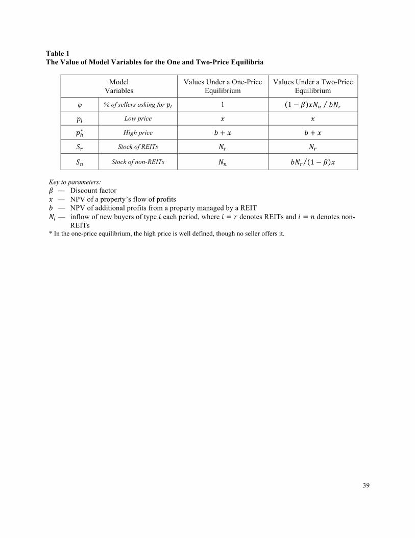
39

Table 1 The Value of Model Variables for the One and Two-Price Equilibria

Model Variables

Values Under a One-Price Equilibrium

Values Under a Two-Price Equilibrium

φ % of sellers asking for !! 1 1 − ! !!!! !!!!

!! Low price ! !

!!∗ High price ! + ! ! + !

!! Stock of REITs !! !!

!! Stock of non-REITs !! !!! 1 − ! ! Key to parameters: ! — Discount factor ! — NPV of a property’s flow of profits ! — NPV of additional profits from a property managed by a REIT !! — inflow of new buyers of type ! each period, where ! = ! denotes REITs and ! = ! denotes non-

REITs * In the one-price equilibrium, the high price is well defined, though no seller offers it.

40

Table 2 Descriptive Statistics—Continuous Variables Commercial Property Transactions in Seven Counties in the Southwestern U.S. (January 1989 through December 2007) Panel A Tests for Distributional Equality of Property Attributes, between REIT and Non-REIT Buyers Variable REIT Means

(471Obs.) Non-REIT Means (139,056 Obs.)

Test Statistics p-value

Sales Price $17,070,273 $2,266,068 910.68 <0.0001 Price Per Square Foot $122.80 $125.52 14.51 0.091 Building Area (SqFt) 166,071 22,713 963.73 <0.0001 Land Area (Acres) 8.22 1.26 979.99 <0.0001 Building Age (Years) 15.67 31.09 73.06 <0.0001 Panel B Descriptive Statistics of Continuous Variables for All Transactions Greater than 20,000 Square Feet. (33,252 Observations) Variable Mean Std Dev Minimum Maximum Sales Price $6,876,326 $13,989,464 $405,000 $435,000,000 Price Per Square Foot $90.63 $74.44 $20.01 $2,052.87 Building Area (SqFt) 72,645 91,466 20,001 2,582,044 Land Area (Acres) 3.77 5.62 0.09 95.00 Building Age (Years) 22.79 16.88 0.00 120.00 Panel C Descriptive Statistics for REIT Transactions Greater than 20,000 Square Feet. (417 Observations) Variable Mean Std. Dev. Minimum Maximum Sales Price $19,113,626 $23,434,397 $670,000 $170,500,000 Price Per Square Foot $107.97 $84.67 $20.03 $806.04 Building Area (SqFt) 186,694 157,347 20,970 974,252 Land Area (Acres) 9.17 9.52 0.10 74.75 Building Age (Years) 14.39 10.33 0.00 73.00 Panel D Descriptive Statistics for Non-REIT Transactions Greater than 20,000 Square Feet. (32,835 Observations) Variable Mean Std. Dev. Minimum Maximum Sales Price $6,720,914 $13,758,877 $405,000 $435,000,000 Price Per Square Foot $90.41 $74.27 $20.01 $2,052.87 Building Area (SqFt) 71,197 89,394 20,001 2,582,044 Land Area (Acres) 3.70 5.52 0.09 95.00 Building Age (Years) 22.90 16.92 0.00 120.00 Notes: The data include transactions of office, retail, industrial, and apartments located within the following southwestern U.S. counties: Clark (NV), Maricopa (AZ), Los Angeles (CA), Orange (CA), Riverside (CA), San Bernardino (CA), and San Diego (CA). The data were obtained from the CoStar Group, Inc.

41

Table 3 Descriptive Statistics—Binary Variables Commercial Property Transactions Greater than 20,000 Square Feet in Seven Counties in the Southwestern U.S. (January 1989 through December 2007)

All Observations REIT Observations Non-REIT Observations Explanatory Variables

No. Obs. % No. Obs. % No. Obs. %

Total Observations 33,252 100 417 32,835 Buyer Location Out-of-State Buyer 6,907 20.77 177 42.45 6,730 20.50 Property Type Office 5,087 15.30 93 22.30 4,994 15.21 Retail 4,717 14.19 41 9.83 4,676 14.24 Industrial 9,810 29.50 119 28.54 9,691 29.51 Apartments 13,638 41.01 164 39.33 13,474 41.04 Transaction Characteristics

REIT Seller 177 0.53 6 1.44 171 0.52 Sale Leaseback 387 1.16 13 3.12 374 1.14 Bank Sale 1,417 4.26 5 1.20 1,412 4.30 RTC Sale 115 0.35 0 0.00 115 0.35 Portfolio Sale 806 2.42 46 11.03 760 2.31 Distress Sale 2693 8.10 17 4.08 2,676 8.15 Exchange (1031) 5,269 15.85 24 5.76 5,245 15.97 County Maricopa, AZ 6,485 19.50 84 20.14 6,401 19.49 Clark, NV 1,977 5.95 25 6.00 1,952 5.94 Los Angeles, CA 13,901 41.81 150 35.97 13,751 41.88 Orange, CA 3,328 10.01 46 11.03 3,282 10.00 Riverside, CA 1,608 4.84 22 5.28 1,586 4.83 San Bernardino, CA 2,139 6.43 30 7.19 2,109 6.42 San Diego, CA 3,814 11.47 60 14.39 3,754 11.43 Year 1989 354 1.06 0 0.00 354 1.08 1990 1,008 3.03 0 0.00 1,008 3.07 1991 786 2.36 4 0.96 782 2.38 1992 966 2.91 12 2.88 954 2.91 1993 1,159 3.49 18 4.32 1,141 3.47 1994 1,410 4.24 32 7.67 1,378 4.20 1995 1,284 3.86 17 4.08 1,267 3.86 1996 1,682 5.06 47 11.27 1,635 4.98 1997 2,088 6.28 88 21.10 2,000 6.09 1998 2,099 6.31 68 16.31 2,031 6.19 1999 2,003 6.02 26 6.24 1,977 6.02 2000 1,933 5.81 10 2.40 1,923 5.86 2001 1,936 5.82 4 0.96 1,932 5.88 2002 2,291 6.89 13 3.12 2,278 6.94 2003 2,676 8.05 17 4.08 2,659 8.10 2004 2,856 8.59 19 4.56 2,837 8.64 2005 2,781 8.36 13 3.12 2,768 8.43 2006 2,212 6.65 19 4.56 2,193 6.68 2007 1,728 5.20 10 2.40 1,718 5.23

Note: Data provided by CoStar Group, Inc.

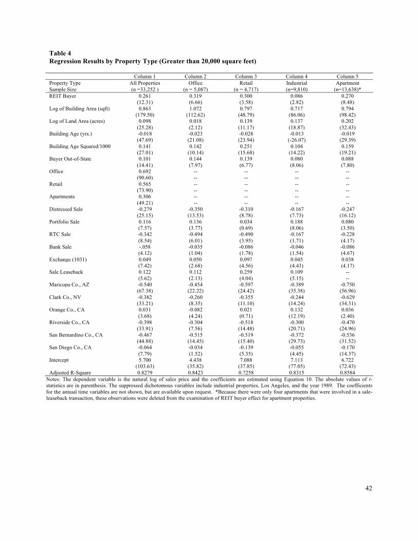
42

Table 4 Regression Results by Property Type (Greater than 20,000 square feet) Column 1 Column 2 Column 3 Column 4 Column 5 Property Type Sample Size

All Properties (n =33,252 )

Office (n = 5,087)

Retail (n = 4,717)

Industrial (n=9,810)

Apartment (n=13,638)*

REIT Buyer 0.261 0.319 0.300 0.086 0.270 (12.31) (6.66) (3.58) (2.82) (8.48) Log of Building Area (sqft) 0.863 1.072 0.797 0.717 0.794 (179.50) (112.62) (48.79) (86.06) (98.42) Log of Land Area (acres) 0.098 0.018 0.139 0.137 0.202 (25.28) (2.12) (11.17) (18.87) (32.43) Building Age (yrs.) -0.018 -0.023 -0.028 -0.013 -0.019 (47.69) (21.08) (23.94) (-26.07) (29.39) Building Age Squared/1000 0.141 0.142 0.251 0.104 0.159 (27.01) (10.14) (15.68) (14.22) (19.21) Buyer Out-of-State 0.101 0.144 0.139 0.080 0.088 (14.41) (7.97) (6.77) (8.06) (7.80) Office 0.692 -- -- -- -- (90.60) -- -- -- -- Retail 0.565 -- -- -- -- (73.90) -- -- -- -- Apartments 0.306 -- -- -- -- (49.21) -- -- -- -- Distressed Sale -0.279 -0.350 -0.310 -0.167 -0.247 (25.15) (13.53) (8.78) (7.73) (16.12) Portfolio Sale 0.116 0.136 0.034 0.188 0.080 (7.57) (3.77) (0.69) (8.06) (3.50) RTC Sale -0.342 -0.494 -0.490 -0.167 -0.228 (8.54) (6.01) (3.95) (1.71) (4.17) Bank Sale -.058 -0.035 -0.086 -0.046 -0.086 (4.12) (1.04) (1.78) (1.54) (4.67) Exchange (1031) 0.049 0.050 0.097 0.045 0.038 (7.42) (2.68) (4.56) (4.43) (4.17) Sale Leaseback 0.122 0.112 0.259 0.109 -- (5.62) (2.13) (4.04) (5.15) -- Maricopa Co., AZ -0.540 -0.454 -0.597 -0.389 -0.750 (67.38) (22.22) (24.42) (35.38) (56.96) Clark Co., NV -0.382 -0.260 -0.355 -0.244 -0.629 (33.21) (8.35) (11.10) (14.24) (34.31) Orange Co., CA 0.031 -0.082 0.021 0.132 0.036 (3.68) (4.24) (0.71) (12.19) (2.40) Riverside Co., CA -0.398 -0.304 -0.518 -0.300 -0.470 (33.91) (7.56) (14.48) (20.71) (24.96) San Bernardino Co., CA -0.467 -0.515 -0.519 -0.372 -0.536 (44.88) (14.45) (15.40) (29.73) (31.52) San Diego Co., CA -0.064 -0.034 -0.139 -0.055 -0.170 (7.79) (1.52) (5.35) (4.45) (14.37) Intercept 5.700 4.438 7.088 7.113 6.722 (103.63) (35.82) (37.85) (77.05) (72.43) Adjusted R-Square 0.8279 0.8423 0.7258 0.8315 0.8584

Notes: The dependent variable is the natural log of sales price and the coefficients are estimated using Equation 10. The absolute values of t-statistics are in parenthesis. The suppressed dichotomous variables include industrial properties, Los Angeles, and the year 1989. The coefficients for the annual time variables are not shown, but are available upon request. *Because there were only four apartments that were involved in a sale-leaseback transaction, these observations were deleted from the examination of REIT buyer effect for apartment properties.

43

Table 5 Regression Results with REIT Seller, Private and Public REITS, and REIT Buyers with New Capital (Greater than 20,000 square feet) Column 1 Column 2 Column 3 Column 4 Column 5

Explanatory Variable Basecase +Public/Private +REIT Size +New Issue + High REIT Presence

REIT Buyer 0.261 -- -- 0.216 0.216 (12.31) -- -- (7.22) (6.15) Public REIT Buyer -- 0.275 -- -- -- -- (12.47) -- -- -- Private REIT Buyer -- 0.095 -- -- -- -- (1.25) -- -- -- Small REIT -- -- 0.093 -- -- -- -- (1.91) -- -- Large REIT -- -- 0.299 -- -- -- -- (6.63) -- -- New Issue -- -- -- 0.089 -- -- -- -- (2.16) -- High REIT Presence -- -- -- -- 0.070 -- -- -- -- (1.62) Log of Building Area (sqft) 0.863 0.863 0.866 0.863 0.863 (179.50) (179.49) (180.36) (179.50) (179.48) Log of Land Area (acres) 0.098 0.098 0.098 0.098 0.098 (25.28) (25.29) (25.24) (25.27) (25.29) Building Age (yrs.) -0.018 -0.018 -0.019 -0.018 -0.018 (47.69) (47.71) (47.83) (47.68) (47.68) Building Age Squared/1000 0.141 0.142 0.142 0.141 0.141 (27.01) (27.03) (27.11) (27.01) (27.00) Buyer Out-of-State 0.101 0.101 0.104 0.101 0.101 (14.41) (14.39) (14.72) (14.41) (14.41) Office 0.692 0.692 0.692 0.692 0.692 (90.60) (90.61) (90.37) (90.62) (90.59) Retail 0.565 0.565 0.565 0.565 0.565 (73.90) (73.87) (73.69) (73.91) (73.89) Apartments 0.306 0.305 0.306 0.305 0.305 (49.21) (49.18) (49.19) (49.18) (49.21) Distressed Sale -0.279 -0.278 -0.281 -0.278 -0.278 (25.15) (25.14) (25.38) (25.13) (25.10) Portfolio Sale 0.116 0.116 0.121 0.115 0.115 (7.57) (7.54) (7.86) (7.55) (7.56) RTC Sale -0.342 -0.342 -0.347 -0.342 -0.342 (8.54) (8.53) (8.65) (8.54) (8.53) Bank Sale -.058 -0.058 -0.059 -0.058 -0.058 (4.12) (4.12) (4.19) (4.13) (4.12) Exchange (1031) 0.049 0.049 0.048 0.049 0.049 (7.42) (7.43) (7.32) (7.44) (7.43) Sale Leaseback 0.122 0.123 0.127 0.122 0.122 (5.62) (5.64) (5.81) (5.61) (5.63) Maricopa Co., AZ -0.540 -0.540 -0.542 -0.540 -0.540 (67.38) (67.38) (67.54) (67.35) (67.39) Clark Co., NV -0.382 -0.382 -0.385 -0.382 -0.382 (33.21) (33.21) (33.36) (33.20) (33.23) Orange Co., CA 0.031 0.031 0.031 0.031 0.031 (3.68) (3.67) (3.67) (3.68) (3.68) Riverside Co., CA -0.398 -0.398 -0.399 -0.397 -0.397 (33.91) (33.92) (33.95) (33.91) (33.91) San Bernardino Co., CA -0.467 -0.467 -0.468 -0.467 -0.467 (44.88) (44.88) (44.91) (44.89) (44.90) San Diego Co., CA -0.064 -0.063 -0.064 -0.063 -0.063 (7.79) (7.76) (7.80) (7.79) (7.78) Intercept 5.706 5.707 5.670 5.706 5.71 (103.63) (103.65) (103.01) (103.64) (103.65) Adjusted R-Square 0.8279 0.8279 0.8273 0.8279 0.8279

Notes: The dependent variable is the natural log of sales price and regressions contain 33,252 observations (real estate transactions). The absolute values of t-statistics are in parenthesis. The suppressed dichotomous variables include industrial properties, Los Angeles, and the year 1989. The annual time variables are not shown, but are available upon request.

44

Figure 1 Fraction of sellers asking for the low price (in the continuous time model) for various parameter values φ = 1 Notes: Each contour indicates the fraction ! of sellers offering the low price for the indicated parameter values of benefit size ! (relative to property value !) and property arrival rate !. The point at (0.82,2) indicates the parameter values used in our numerical example. For instance, the boundary labeled 0.1 (the border between the two darkest regions) represents all parameter combinations for which 10% of sellers ask the low price in a two-price equilibrium. In contrast, the white region represents parameters for which the single-price equilibrium occurs, with 100% of sellers asking the low price.

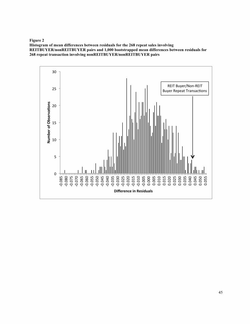
45

Figure 2 Histogram of mean differences between residuals for the 268 repeat sales involving REITBUYER/nonREITBUYER pairs and 1,000 bootstrapped mean differences between residuals for 268 repeat transaction involving nonREITBUYER/nonREITBUYER pairs

0"

5"

10"

15"

20"

25"

30"

'0.085

"'0.080

"'0.075

"'0.070

"'0.065

"'0.060

"'0.055

"'0.050

"'0.045

"'0.040

"'0.035

"'0.030

"'0.025

"'0.020

"'0.015

"'0.010

"'0.005

"0.000"

0.005"

0.010"

0.015"

0.020"

0.025"

0.030"

0.035"

0.040"

0.045"

0.050"

0.055"

Num

ber'o

f'Observa.o

ns'

Difference'in'Residuals'

REIT"Buyer/Non'REIT""Buyer"Repeat"Transac?ons"

"