Embed Size (px)
Citation preview

© Pilot Publishing Company Ltd. 2005
Chapter 13
Factor Market

© Pilot Publishing Company Ltd. 2005
Contents:
• Factor Demand
• Factor Supply
• Other Points to be Noticed

© Pilot Publishing Company Ltd. 2005
Factor Demand
© Pilot Publishing Company Ltd. 2005
In factor markets
Firms demand factors to produce goods
Firms aims at maximizing wealth (by weighing
the gain from employing factors against the cost.)

© Pilot Publishing Company Ltd. 2005
Factor demand
is also called derived demand.
Because a firm demands factors only if there is
a demand for the good it produces.
© Pilot Publishing Company Ltd. 2005
Symbols:
Quantities of factors employed – A, B, C, ...
Factor (hire) prices – HA, HB, HC, ... Quantity of the good produced (product) – Q
Product price – P
© Pilot Publishing Company Ltd. 2005
Marginal factor cost (MFC)
Marginal factor cost curve
is the cost of employing an additional unit of a factor.
(MFC of a factor vs. MC of a good)

© Pilot Publishing Company Ltd. 2005
Marginal factor cost curve
Assumptions:
1. The firm is a price-taker in the factor market.
2. It cannot affect the prevailing factor price (H) & hence MFC is a constant equal to H.
MFC = H (=AFC)
© Pilot Publishing Company Ltd. 2005
Factor Supply Curve
= MFC curve = AFC curve
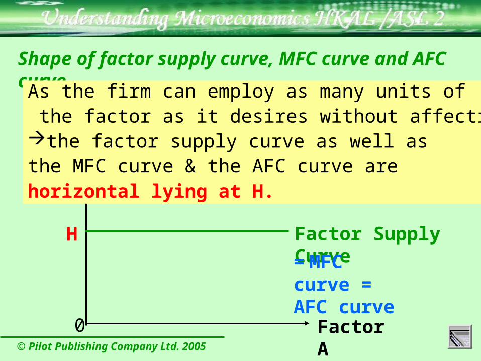
Shape of factor supply curve, MFC curve and AFC curve
$
Factor A0
H
As the firm can employ as many units of the factor as it desires without affecting H,the factor supply curve as well asthe MFC curve & the AFC curve arehorizontal lying at H.
© Pilot Publishing Company Ltd. 2005
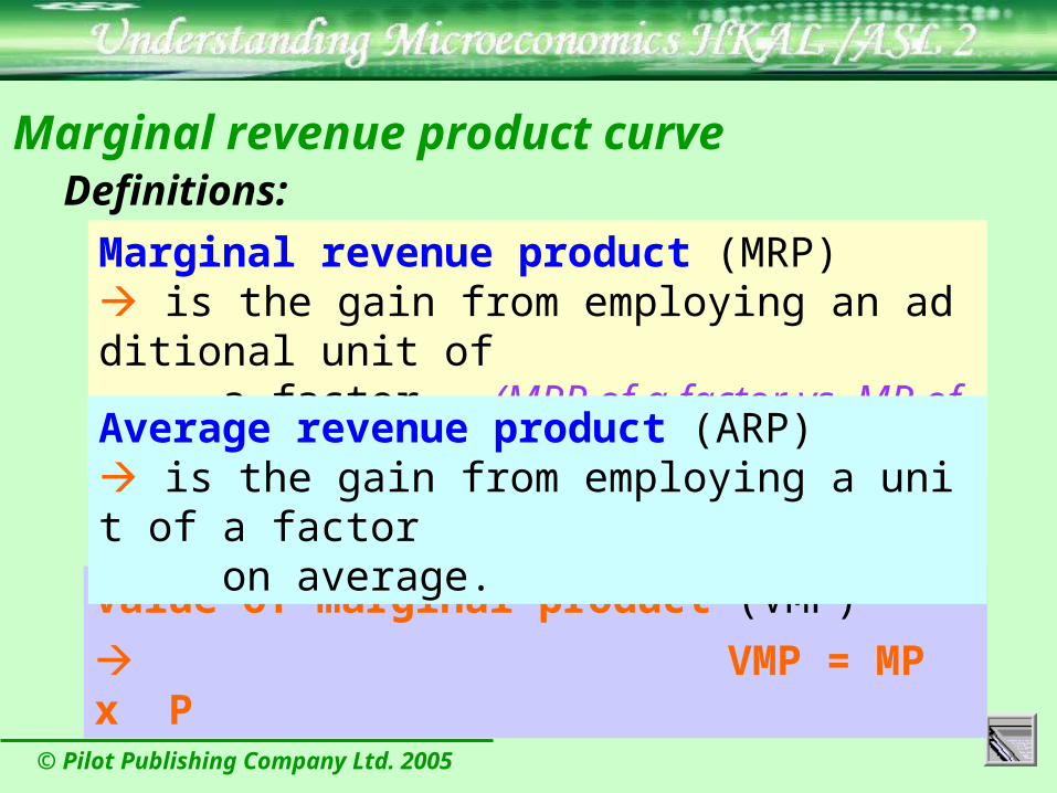
Marginal revenue product curve
Value of marginal product (VMP)
VMP = MP x P
Marginal revenue product (MRP) is the gain from employing an additional unit of a factor. (MRP of a factor vs. MR of a good)
Average revenue product (ARP) is the gain from employing a unit of a factor on average.
Definitions:
© Pilot Publishing Company Ltd. 2005
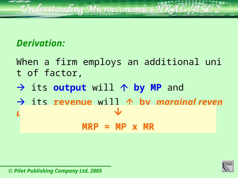
When a firm employs an additional unit of factor,
its output will by MP and
its revenue will by marginal revenue product
Derivation:
MRP = MP x MR
© Pilot Publishing Company Ltd. 2005
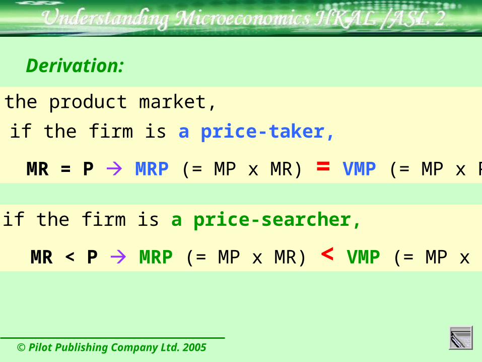
In the product market,
if the firm is a price-taker,
MR = P MRP (= MP x MR) = VMP (= MP x P)
if the firm is a price-searcher,
MR < P MRP (= MP x MR) < VMP (= MP x P)
Derivation:

© Pilot Publishing Company Ltd. 2005
APMP
Output produced
0 Factor A 0
ARP=AP x AR
MRP=MP x MR
Factor A
Output produced
Shape of MRP curve and ARP curve
AP x AR=ARP
MP x MR=MRP
Derivation of MRP and ARP curve
© Pilot Publishing Company Ltd. 2005
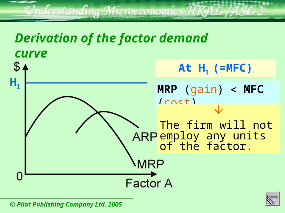
H1 MRP (gain) MFC (cost)
The firm will not employ any units of the factor.
At H1 (=MFC)
Derivation of the factor demand curve
© Pilot Publishing Company Ltd. 2005
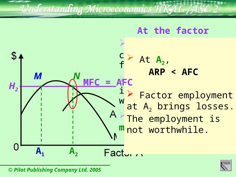
H2
M
A1
N
A2
At the factor price of H2
At M, MRP curve cuts MFC curve from below.
Either an or in factor employment would raise wealth.
A1 is wealth-
minimizing.
At N, MRP curve cuts MFC curve from above.
Either an or in factor employment would reduce wealth.
A2 is wealth-maximizing
At A2, ARP < AFC
Factor employmentat A2 brings losses. The employment is not worthwhile.
MFC = AFC
© Pilot Publishing Company Ltd. 2005
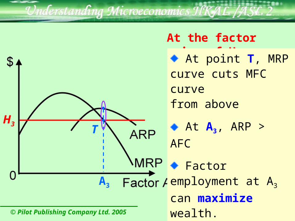
H3
A3
T
At the factor price of H3
At point T, MRP curve cuts MFC curve from above
At A3, ARP > AFC
Factor employment at A3 can maximize wealth.

© Pilot Publishing Company Ltd. 2005
Equilibrium conditions of factor employment
1. MRP = MFC1. MRP = MFC
2. MRP curve cuts MFC curve from above
(to determine the best employment level)
2. MRP curve cuts MFC curve from above
(to determine the best employment level)
3. ARP AFC
(to determine if it is worth employing)
3. ARP AFC
(to determine if it is worth employing)
© Pilot Publishing Company Ltd. 2005
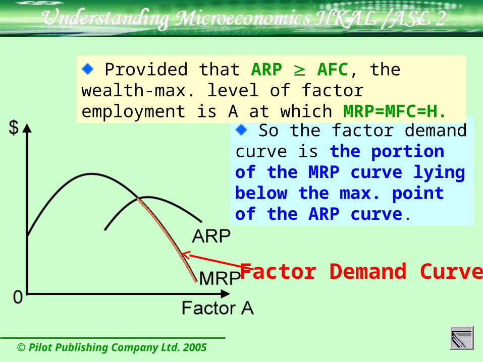
So the factor demand curve is the portion of the MRP curve lying below the max. point of the ARP curve.
Provided that ARP AFC, the wealth-max. level of factor employment is A at which MRP=MFC=H.
Factor Demand Curve

© Pilot Publishing Company Ltd. 2005
Market factor demand curve
A factor is demanded by many different firms, e.g., clerks are employed in hospitals, schools, accounting firms, etc.
So the market factor demand curve is equal to the horizontal sum of factor demand curves of all the firms in the market.

© Pilot Publishing Company Ltd. 2005
Factor Supply

© Pilot Publishing Company Ltd. 2005
Income
Resource for own use (e.g., leisure)
N
M
R0R0 (e.g., 24 hours)
I0
Numerical value of the slope = Factor price (e.g., hourly wage rate)
Budget line of a price-taking factor supplier
© Pilot Publishing Company Ltd. 2005
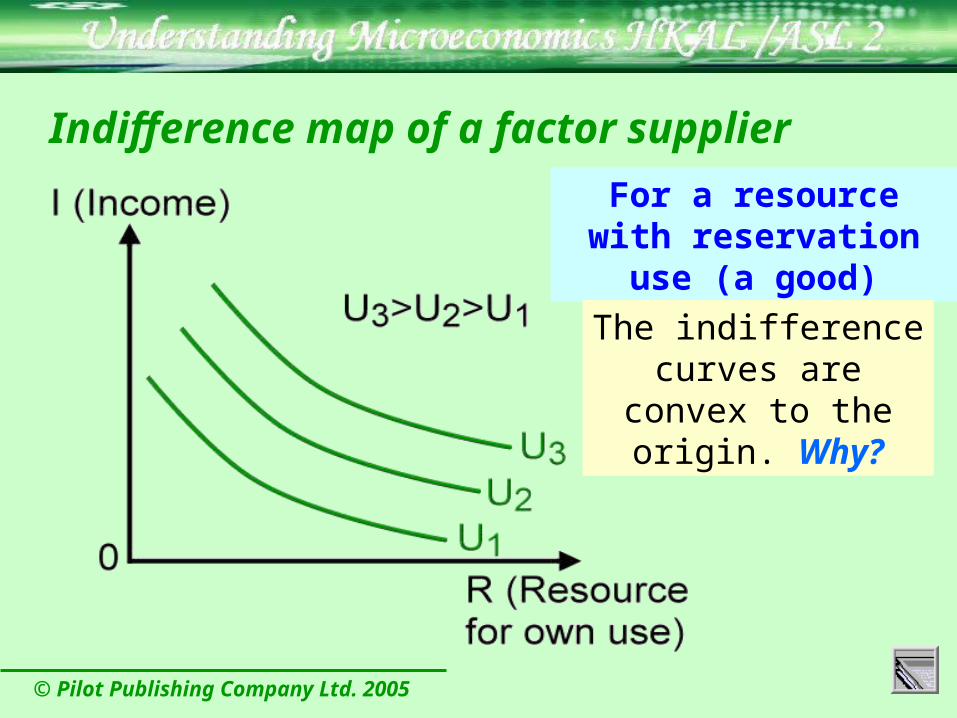
Indifference map of a factor supplier
For a resource with reservation use (a good)
The indifference curves are convex to the
origin. Why?
© Pilot Publishing Company Ltd. 2005
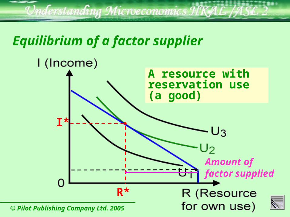
Equilibrium of a factor supplier
I*
R*
A resource with reservation use (a good)
Amount of factor supplied

© Pilot Publishing Company Ltd. 2005
in price
Budget line tilts upward
Price effect
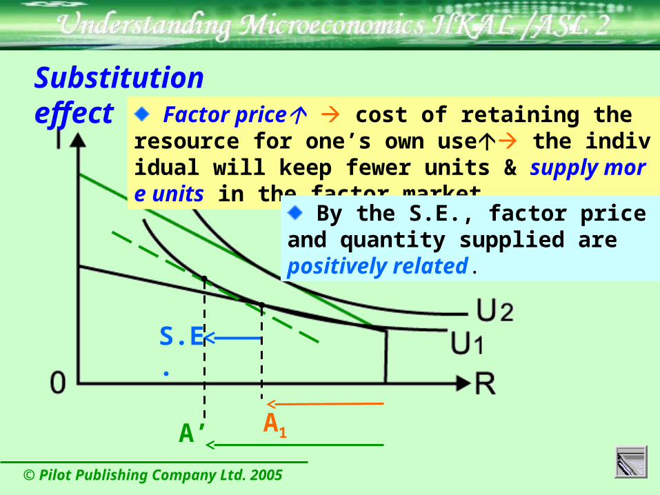
Substitution effect and income effect of a price change
The effect of a change in price can be decomposed into substitution effect and income effect.
A1A2
© Pilot Publishing Company Ltd. 2005
S.E.
Substitution effect Factor price cost of retaining the resource for o
ne’s own use the individual will keep fewer units & supply more units in the factor market.
By the S.E., factor price and quantity supplied are positively related.
A1A’
© Pilot Publishing Company Ltd. 2005
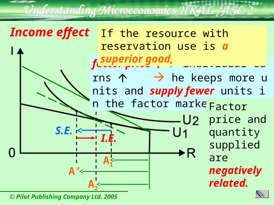
S.E.
A1A’
A2
Income effect
I.E.
factor price individual earns he keeps more units and supply fewer units in the factor market.
If the resource with reservation use is a superior good,
Factor price and quantity supplied arenegatively related.
© Pilot Publishing Company Ltd. 2005
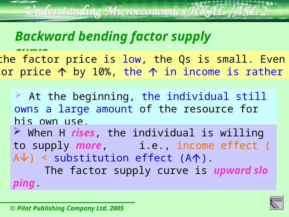
Backward bending factor supply curve
When the factor price is low, the Qs is small. Even if the factor price by 10%, the in income is rather small.
At the beginning, the individual still owns a large amount of the resource for his own use.
When H rises, the individual is willing to supply more, i.e., income effect (A) < substitution effect (A). The factor supply curve is upward sloping.
© Pilot Publishing Company Ltd. 2005
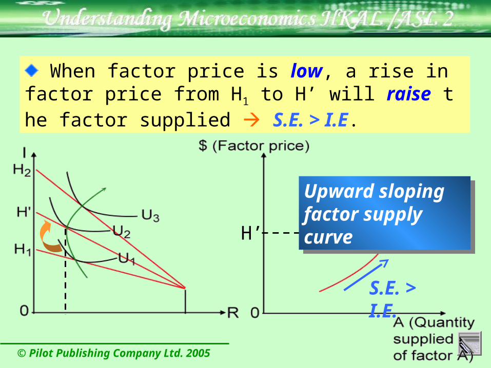
H’
S.E. > I.E.
When factor price is low, a rise in factor price from H1 to H’ will raise the factor supplied S.E. > I.E.
Upward sloping factor supply curve
Upward sloping factor supply curve

© Pilot Publishing Company Ltd. 2005
Backward bending factor supply curve (con’t)
When the factor price is high, the Qs is large. Even a 10% rise in income will raise the income by a very large amount.
The individual now owns only a very small amount of the resource for his own use.
This time, when H rises, the individual desires to keep more units of the resource for his own use & supply less, i.e., income effect (A) > substitution effect (A). The factor supply curve is downward sloping.
© Pilot Publishing Company Ltd. 2005
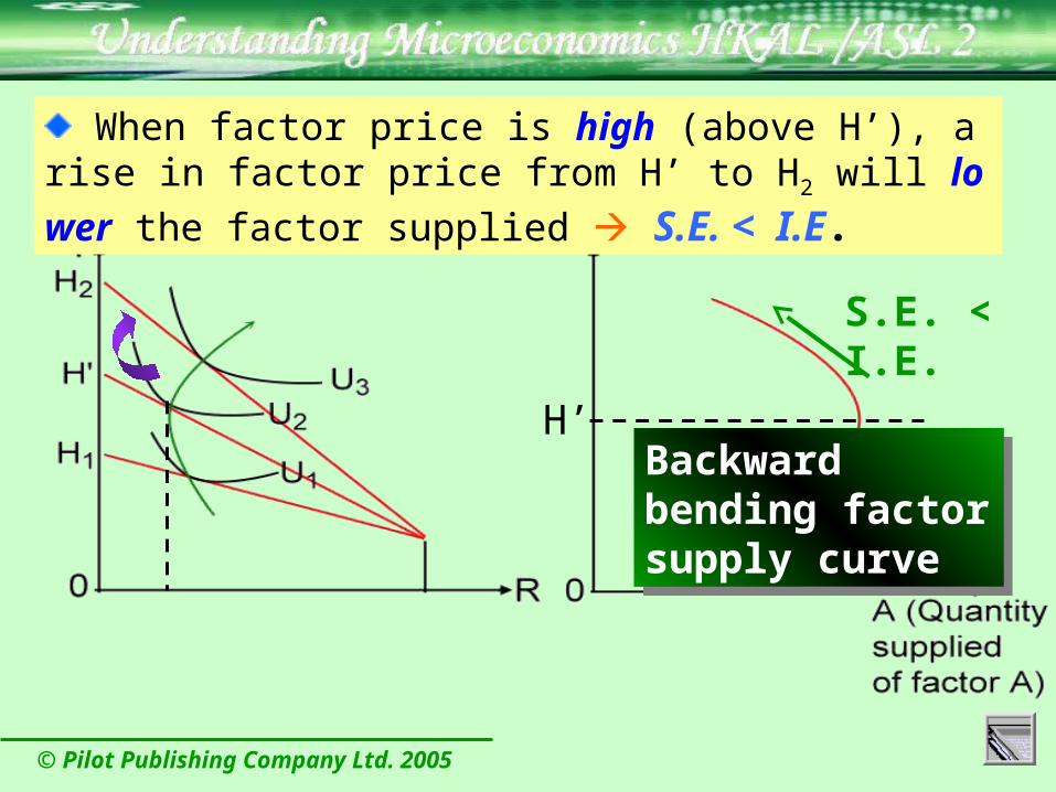
H’
S.E. < I.E.
Backward bending factor supply curve
Backward bending factor supply curve
When factor price is high (above H’), a rise in factor price from H’ to H2 will lower the factor supplied S.E. < I.E.

© Pilot Publishing Company Ltd. 2005
Q13.3:
If the resource with reservation use is an inferior good, what will be the shape of the factor supply curve of an individual?

© Pilot Publishing Company Ltd. 2005
Other Points to be Noticed

© Pilot Publishing Company Ltd. 2005
Total payment to labour (W x L)Total payment to
other factors (TRP – W x L)
Total receipt (TRP = ARP x L)
Functional distribution of income
$
ARP
MRP
MFC=AFCW
0 LQuantity supplied of labour
© Pilot Publishing Company Ltd. 2005
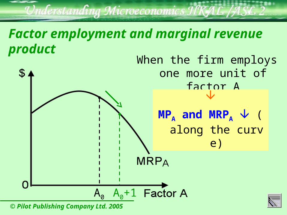
Factor employment and marginal revenue product
When the firm employs one more unit of factor A
MPA and MRPA (along the curve)
A0 A0+1
© Pilot Publishing Company Ltd. 2005
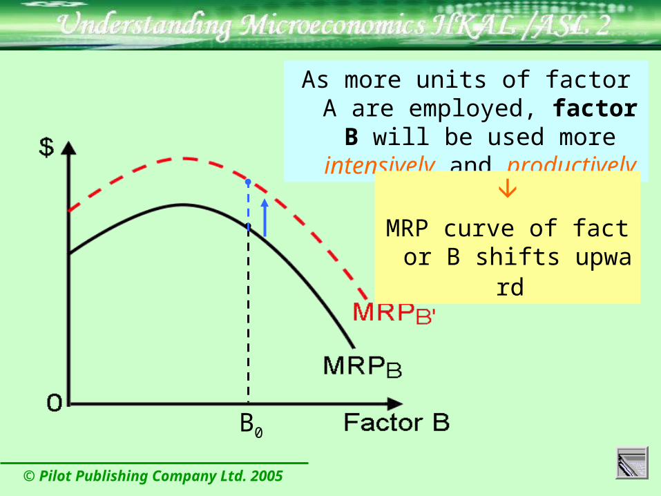
B0
As more units of factor A are employed, factor B will be used
more intensively and productively
MRP curve of factor B shifts upward

© Pilot Publishing Company Ltd. 2005
Malthus’ law of population – a myth?
Population living standard of man (since MP & AP ) Population cease to expand when AP to the subsistence level
Malthus’ law of population

© Pilot Publishing Company Ltd. 2005
Why is the law not confirmed? Capital accumulation
MP & AP curve shifted upward greatly & rapidly.
Average living standard rose with population growth.
Investment on education Technological improvement Institutional improvement Specialization due to globalization
© Pilot Publishing Company Ltd. 2005
Income differential
In a price-taking factor market,
price of a factor (factor income) is determined by
the market D & S of the factor.

© Pilot Publishing Company Ltd. 2005
Income differential
market demand is determined by
In a price-taking factor market,
productivity of the factor
(e.g., ability, training and working experience)
price of the product (depends on its D & S),
discrimination
(e.g., against the female, youngster & minority)

© Pilot Publishing Company Ltd. 2005
Income differential
market supply is determined by
In a price-taking factor market,
amount of capital accumulated
size & structure of population
geographical distribution of labour
government policies
power of trade union
© Pilot Publishing Company Ltd. 2005
If the factor market is price-searching, (or controlled by a central authority / an institution)
factor price is NOT determined by the market D & S of the factor
H may not reflect the productivity of the factor
i.e., H MRP.
© Pilot Publishing Company Ltd. 2005
Correcting Misconceptions:
1. MRP is the same as VMP.
2. The demand curve for a factor is the MRP
curve.
3. If a firm is a price-taker in a factor market,
the factor demand curve is horizontal.
4. Substitution effect must be negative.

© Pilot Publishing Company Ltd. 2005
5. The higher the factor price, the larger the quantity supplied of a factor.
6. As the average living standard rises with population growth, the law of diminishing returns is falsified.
7. The hire price of a factor must reflect its marginal productivity.
Correcting Misconceptions:

© Pilot Publishing Company Ltd. 2005
Survival Kit in Exam:Question 13.1: Presently, a firm employs five workers. When the workers are on their sick leave, the value of their output drops. The table below shows the situation. If the wage rate is $650, how many workers should the firm employ?
No. of workers on their sick leave
Drop in the value of their output
1 $500
2 $1 100
3 $1 800
4 $2 600
5 $3 500

© Pilot Publishing Company Ltd. 2005
Survival Kit in ExamQuestion 13.2:Suppose a firm employs only two factors, land and labour. The total return is distributed among them. If the firm fires several workers, what will happen to
(a) the marginal product of labour and that of land?
(b) the total return of labour and that of land?