Embed Size (px)
Citation preview

“W.
'U
'3"(‘0
O'|U|u'|"‘"\
.0"‘l‘f$|r.l
0".0.)
-.v_.
I(’u''M
"'3"'J
'.‘u'l'
''
''
'r'
‘'*
o'.‘“
'‘
‘"
"I
‘3':
‘.
IH
n'
‘l
- a
I‘I‘Q-‘o
O
“‘0‘“ 0
.‘n
4‘\~_
v Ag.‘
‘*74?:
v.
,‘
g\
~60
-o
{W
b
"om-Min
0‘..oa'.‘.'4'.
.9'.
''
-
--¢
'.
0..‘-.'.
....
n,
-.'4‘.fx_
:"'
'"vy...
~
.~\-
at
'.
u‘.
‘5
...
‘'
1“v§.‘>,\..
‘".o
..
’-
h'u
"i'
I4|.o
‘
‘.
.Aggi'uw
‘f.n.
sh
\‘."I\.'
Conr‘v.
c'.\_.
.Z
‘‘tu.
.A-
\"‘
‘
'‘3
:.
“0‘h‘.¥
V‘
'I|
D.
.
"‘‘\'
3.9:7‘0\~-
'O-
'I:.‘-I.
.|.‘R
....\.
\u
I.
.
0.
I...“C
I.
1..
.lat.
a“
I
'
v
t'
.
.~.,
.-0
"'-n
o.
_
"U.”
‘s'fi
‘-
.'
''
-
..
.n
0....
"1"‘
""’|
.-01.1
.It
.I..
..
»JIII.4....‘0V.I
.-"~
...
._.
u.
h.
.,.
r“...
L.._
.._|..
“HI",
..huo.
.“
.
Thesis for the De
MICHIGAN STATE UNIVERSITY
”-ILLIAM e. RUESINK
11970
gree. of
o
a
M. S;
o
r
O[:13
‘\
u
I‘
O-
l-.0
A.
a
O.0'01-
—A
‘_
44
44
”flow-no.9..n‘ ‘0'.“ “.‘..o o
SWEEPNET D.
ETERMJ f - - TSGN 0F PU
.
v
.
[A
-wv.o.....4.. 9.0.0'NQ‘0 ”fl'fliufigv‘
.
.vf—‘wv'
o
. o
o
r...
.
..l
n.
4.
,.‘.',"~‘
1‘
'1':
‘0
,v~c-¢¢.g.,.4...0
'0‘ A

FCH‘
LIBRARY ‘
Michigan State ‘
University

ABSTRACT
SWEEPNET DETERMINATION OF POPULATION DENSITIES OF THE
CEREAL LEAF BEETLE, Oulema melanopus (L.)
By
William G. Ruesink
Two interrelated models were developed to predict cereal leaf
beetle density from sweepnet catch. The mathematical model requires
knowledge of sweepnet diameter, length of stroke, the proportion of the
insect population that is in the net's path, and the probability of
capture given that the insect is in the net's path. Difficulty in
submodeling the last two variables led to the development of an alter-
native regression model. This model is specific to adult cereal leaf
beetles and assumes a 15" net and a 5' stroke. It requires knowledge
of wind speed, temperature, solar radiation intensity, and crop height.
The regression has an r2 of 0.87.
Variance analysis showed that between field variance is much
greater than within field variance and that the difference increases
as density increases. Optimal allocation of sampling resources re—
quires one sample per field and as many fields as possible with those
resources. Normally if 60% of the fields of one crop in an area are
sampled, then for that crop the standard error of the catch is within
10% of the mean.

SWEEPNET DETERMINATION OF POPULATION DENSITIES OF THE
CEREAL LEAF BEETLE, Oulema melanopus (L.)
By
1.
William GE‘Ruesink
A THESIS
Submitted to
Michigan State University
in partial fulfillment of the requirements
for the degree of
MASTER OF SCIENCE
Department of Entomology
1970

ACKNOWLEDGEMENTS
My sincere appreciation is extended to Dr. Dean Haynes whose
direction and inspiration made the completion of this work possible.
He very ably introduced me to entomological research, a job that was
complicated by the fact that my background was in mathematics and not
entomology.
The other members of my guidance committee also deserve credit
for their contributions to my program: Dr. Gordon Guyer for his per-
petual optimism, Dr. Robert Ruppel for his experience with the cereal
leaf beetle since its discovery in the United States, Dr. William
Cooper from the Department of Zoology for emphasis of quantitative
precision, and Mr. Richard Connin from the United States Department of
Agriculture for providing the equipment needed in this study.
ii

TABLE OF CONTENTS
LIST OF TABLES O O O O O O O O O O O O O O O O O O O 0
LIST OF FIGURES O O O O O O O O O O O O O O O O O O O
INTRODUCTION 0 O O O O O O O O O O O O O O O O O O O 0
LITERATURE REVIEW . . . . . . . . . . . . . . . . . .
METHODS
RESULTS
DISCUSS
The Cereal Leaf Beetle . . . . . . . . . . . .
Sweepnet Sampling of Insect Populations . . . .
AND MATERIAI‘S O I O O O O C O O O O O O I O O
Thumbtack Test of the Mathematical Model . . .
Measurement of Absolute Density . . . . . . . .
Vertical Distribution . . . . . . . . . . . . .
Wind Profile . . . . . . . . . . . . . . . . .
Sweepnet Catch . . . . . . . . . . . . . . . .
Variance Components . . . . . . . . . . . . . .
Development of the Proposed Mathematical Model
Thumbtack Test of the Model . . . . . . . . . .
Vertical Distribution of the Cereal Leaf Beetle
Wind Profile . . . . . . . . . . . . . . . . .
Converting Sweepnet Catch to Absolute Density .
Components of Variance Involved in Estimating
Cereal Leaf Beetle Density . . . . . . . . .
ION O O O O I O O O O O O O O O O O O O O O O 0
Mathematical Model . . . . . . . . . . . . . .
Regression Model . . . . . . . . . . . . . . .
Comparing the TWo Models . . . . . . . . . . .
Vertical Distribution . . . . . . . . . .
Optimal Number of Samples Within Each Field . .
Optimal Number of Fields per Township . . .
Exceptional‘Cases . . . . . . . . . . . . . . .
iii
Page
vi
oouw
oooooooo
tars
12
13
15
15
18
24
30
30
31
33
34
35
36
38

CONCLUSIONS . .
LITERATURE CITED
APPENDIX . . . .
iv
Page

10.
ll.
12.
LIST OF TABLES
Test of the Sweepnet Model Using Thumbtacks as
Artificial Insects: 99 Samples of 10 Sweeps Each .
Difference in Vertical Distribution of the Four
Larval Instars in 38" Wheat . . . . . . . . . . . .
Observed Values of the Multiplication Factor M and
the Associated Physical Conditions for Adult
Cereal Leaf Beetles . . . . . . . . . . . . . . . .
Statistics of the Mu1tiple Regression for
Predicting M I O 0 O O O O O C I O O O O O O O O 0
Observed Values of the Multiplication Factor M
for Cereal Leaf Beetle Larvae and the Associated
PhYSical Factors 0 O O O O O O O O O O O O O O I 0
Regression Statistics for Predicting Within and
Between Field VAriances from Mean Catch per Sample
Within and Between Field Variance as Predicted
From the Regression Equations . . . . . . . . . .
Computed Values for the Factor b for Various
Heights of the Sweepnet Rim Above the Ground,
and for the Particular Vertical Distribution
Shown in Figure 2 . . . . . . . . . . . . . . . . .
Predicted Number of Fields to Sample for Certain
Values of NF and a . . . . . . . . . . . . . . .
Grain Row Direction in Relation to Sweeping
Direction as it Affects Sweepnet Catch of
Spring Adults 0 O O O O O O O O O O O O O O O O 0
Comparison of Sweepnet Catch of Summer Adults
Inside and Outside the Sampling Cage . . . . . . .
Within Field Variation in Sweepnet Catch . . . . . .
V
Page
14
18
20
23
25
27
29
32
38
46
47
48

LIST OF FIGURES
Figure Page
1. Spread of the Cereal Leaf Beetle . . . . . . . . . . . . . 4
2. Six Cases of Cereal Leaf Beetle Vertical
Distribution . . . . . . . . . . . . . . . . . . . . . . 16
3. Change in Wind Speed with Height Above Ground
in 5" oats and in 20" Wheat 0 O O O O O O O O O O O O O O 17
4. Relationship Between Mean Catch per Sweep and
the Variance Around that Mean for Within Field
and Between Field Samples . . . . . . . . . . . . . . . . 28
5. Catch per 100 Sweeps in Ten Regions of an Oat
Field Adjacent to an Apple Orchard . . . . . . . . . . . 39
6. Catch per 50 Sweeps Along Three Transects in
Wheat Adjacent to Oats (Spring Adults) . . . . . . . . . 39
vi

INTRODUCTION
One of the most basic problems in quantitative population ecology
is the accurate estimation of the number of individuals in a population.
The solution is seldom simple. If the population is small and well
defined, then census methods might be used. However, in most cases some
type of sampling program is the only realistic approach. Then the
answer must be presented as a best estimate with an associated error
term. In general if the population must be estimated very accurately,
then the sampling program will involve direct counts of individuals per
unit area. When slightly less accuracy is required but large areas must
be surveyed, then a program using a population index rather than direct
counts will result in substantial savings of both time and effort. The
catch of the traditional sweepnet is an example of such an index.
Two interrelated goals were established for this study. First
it was necessary to relate sweepnet catch to absolute density. The
aim was to predict accurately the number of cereal leaf beetles per
square foot from sweepnet catch. Since insects are not uniformly dis-
tributed in the environment, several samples per field would be needed
to accurately establish their density for that field. Furthermore,
several fields should be sampled to accurately estimate density for
the entire township. The second goal, therefore, was a method of
assessing the accuracy with which the field and township densities were
1

2
estimated once the data were in, or alternatively, specifying the
amount of sampling necessary to obtain a given accuracy.
The principal application of the sampling methods developed
here will be to measure the between generation changes in the cereal
leaf beetle population. Since this insect moves moderately long dis-
tances within its lifetime (probably several miles), any measure of
natural population change between generations must involve sampling
a large area. The results in this thesis will provide the necessary
tools to use sweepnet sampling for estimating the annual generation
changes and to know the accuracy of that estimate.

LITERATURE REVIEW
The Cereal Leaf Beetle
Published accounts of the life history of the cereal leaf beetle
can be found in Ruppel (1964), Castro gt_§l, (1965), Yun (1967), and
Helgesen (1969). This univoltine beetle overwinters as an adult. In
the spring mating occurs followed by oviposition on small grains and
to a lesser extent on native grasses. The larvae pass through four
instars reaching a peak density in mid-June. Pupation occurs in the
soil, and the new adults emerge in early July.
The cereal leaf beetle is of European origin. Yun (1967) reports
that farmers in southwestern Michigan were spraying their oats for this
pest as early as 1959 although it remained unidentified until 1962.
A preliminary survey in 1962 showed four counties were infested. Since
then it has spread (see Figure 1) east to central New York state, north
to the Straits of Mackinaw, south into central Kentucky, and west to
central Illinois (USDA, 1969). The slow westward movement is attributed
by Shade and Wilson (1964) to the prevailing westerly winds.
Sweepnet Sampling of Insect Populations
Excellent reviews on sampling insect populations can be found in
Morris (1960) and Southwood (1966). Both authors recognized three
major types of population sampling: absolute (or direct), indirect,
and population index. Absolute sampling entails directly counting
3

Figure
l.--Spread of the Cereal Leaf Beetle.
\\\\\\1966-1968
5
every individual in a unit area of the earth's surface. Indirect
sampling utilizes some technique such as mark-recapture so that not
all individuals on the unit area need be counted. Population index
sampling simply requires measurement of some factor related to density.
Sweepnet catch is a population index that has been used for over
a century (Bremi-Wolf, 1846). Very little was written about its
quantitative use until DeLong (1932) reported on some problems he en-
countered using the sweepnet to estimate population density. He re—
ported that the proportion of the population caught varied with tempera—
ture, humidity, wind, sun angle, plant size and condition, height
swept, rapidity and length of stroke, and whether the sweep strokes
went with or across the grain rows.
Romney (1945) studied the effect of physical factors on sweep-
net catch of the beet leaf hopper on Russian thistle in New Mexico.
Host height, cloud cover, host plant density, time of day, and humidity
had no effect on catch. In his tests host height never exceeded net
diameter. If it had, he states, then host height may have become
important. Temperature and wind velocity did have important effects,
catch being directly pr0portional to temperature and inversely pro-
portional to wind velocity.
Hughes (1955), in a study of a chloropid fly in wheat, found
wind to be the only significant factor affecting sweepnet catch with
temperature, humidity, and solar radiation having negligible effects.
Menhinick (1963) was interested in converting sweepnet catch to
density. He presented the equation:
Zlm
:4»a

where S = number of net strokes
N = number of insects caught in the N strokes
T = number of insects in the area A
A = area of region swept (in m2)
M = number of sweeps necessary to catch the insects on one 1112
Then be calculated values of M for several insect species swept from
lespedeza and found that they ranged from 2.3 to 10.8 dependent on
species and weather. For the one chrysomelid beetle in his list M
averaged 4.9 and varied only slightly with weather. The M values were
then used on other data to convert catch per sweep (i.e. N divided by
S) into density (i.e. T divided by A).
Another aspect of the quantitative study of the sweepnet is to
relate the number of sweeps to the accuracy of the estimated density.
In a sequence of publications (Gray and Treloar, 1933; Beall, 1935;
and Gray and Treloar, 1935) dealing with several species of insects
swept from alfalfa, the authors show that accuracy increases with
number of sweeps and with insect density. Hence if the degree of
accuracy is specified, the number of sweeps required increases as den-
sity decreases. Specifically they found that 775 sweeps at 3.4 insects
per sweep or 6750 sweeps at 0.07 insects per sweep would give an esti-
mate of mean density within 10% of the mean in 95% of the cases. They
concluded that sweepnet catch is too variable to be useful as a census
technique.
Banks and Brown (1962) compared the sweepnet to quadrat counts
and the mark-recapture technique in sampling a hemipterous bug in
wheat. Using as a criterion that the standard error be within 10% of

7
the sample mean, they showed that 100 quadrats of l m2 each, or marking
and recapturing on an area of 1000 m2, or taking 1200 sweeps each met
the criterion. The sweepnet method required the fewest man—hours.

METHODS AND MATERIALS
Thumbtack Test of the Mathematical Model
A deterministic mathematical model was hypothesized and tested
using thumbtacks as artificial insects. An area of 18,000 square feet
within a headed oat field was marked off in mid-July. Each thumbtack
was stuck into a flag leaf near its midrib and about 3 inches from its
base. They were placed roughly 12" apart down every sixth row. Rows
being 7" apart meant the thumbtacks were spaced approximately every
12" by 42". A total of 4867 thumbtacks were so placed. Four men with
12" sweepnets swept the field across the rows, taking 10 strokes of
5 feet each, then emptying the catch into pint ice cream cartons
labeled to indicate the sweeper and sample number. In another part of
the same field 40 thumbtacks were placed in one row some 2 feet apart,
again in the flag leaf as described above. This row was carefully
swept so that the net met each thumbtack squarely and directly.
Measurement of Absolute Density
Three different methods were used to measure absolute density
of the cereal leaf beetle in the field. Each was designed to Operate
under different circumstances.
Adult sampling: Two men dropped a cage (6.5' x 6.5' x 6' high,
open bottom) over the area to be sampled. The cage was entered through
a zipper door, three strokes taken with the sweepnet, and the remaining
8

beetles removed by hand aspiration. The cage was then moved to another
sampling site.
Larval sampling: One square yard of grain was clipped, put
into a plastic bag, and returned to the lab for counting.
High density sampling: Each sample consisted of one row of
grain 24" long selected by throwing a 24" wooden stick into the field,
then moving 4 feet down the row indicated. This moving assured an
undisturbed sample site. As the sample unit was small, it was practical
to count the sample in the field. This method was also applicable to
adults when temperatures were below 65°F (i.e. escape by flight was
unlikely).
Vertical Distribution
The method described above under "High density sampling" was
used when sampling for adult vertical distribution. Within each sample
the height above ground for each beetle was recorded.
Vertical distribution of larvae was recorded in a similar manner
except that samples of longer than 2 feet of row were taken. Five
separate sets of data were recorded, one for each instar and another
for total larvae.
Wind Profile
On May 16, 1968 at Galien, Michigan wind speeds were measured
in wheat and in oats at 2", 9", l6", 4', and 6-1/2" above the ground.
Three measurements of one minute each were taken using a vane
anemometer .

10
Sweepnet Catch
All sweepnet samples were taken by the author with a 15"
sweepnet using 5' strokes. In addition to recording the catch, data
were taken on the number of sweeps, host crop species and height,
location, and date. Data regarding weather conditions were taken from
hygrothermographs and pyrheliographs at both Galien and Gull Lake,
Michigan. Galien also had a recording cup anemometer. Elsewhere these
data were obtained from weather bureau records.
The hypothesis of DeLong (1932) that sweepnet catch may vary
with direction of sweeping (i.e. with or across the grain rows) was
tested with spring adults in wheat. Each sample consisted of 10
sweeps with 14 samples taken across the rows and 16 with the rows.
It was suspected that placing the sampling cage as described
above might affect the behavior of the beetles and hence affect the
catch from the sweeps taken inside the cage. To test this hypothesis
an identical 3 sweep sample was taken outside the cage. Twenty-three
such paired samples were taken over a period of several days.
Variance Components
Within field variance was estimated from numerous small samples
within each field. Each sample consisted of a number of sweeps,
usually taken along a transect. In several fields samples were taken
at points uniformly distributed across the field. The number of sweeps
per sample was constant for any one set of samples but varied between
sets from one to 50. Both adults and larvae were sampled from oats,
barley, wheat and corn. For each field sampled the mean catch per
sample and the variance around that mean were computed.

11
A component including within field variance and between field
variance was calculated from data obtained from the Cooperative Cereal
Leaf Beetle Survey of 1967 and 1968. That survey covered 16 townships
in Michigan, Ohio, and Indiana, and within each township 196 fields
were sampled regularly throughout the season. The mean catch per sample
and the variance around that mean were calculated from sets of data
points chosen to include only within and between field variances.
Within each data set date, crop, collector, and township were constant
and time varied less than 3 hours and temperature less than 10°F.

RESULTS
Development of the Proposed
Mathematical Model
This model predicts average expected catch per sweep as a
function of five variables. Since the model is deterministic rather
than stochastic no prediction is made for variance. The pr0posed
model is:
C = dLDbp (1)
where C = Number of individuals caught per sweep
d = Diameter of the sweepnet Opening (in feet)
L = Length of each stroke of the net (in feet)
D = Density of the individuals being caught (number per
square foot)
b = Proportion of the population that is in the sweepnet's
path
p = Probability of getting into the sweepnet given that
the individual is in the sweepnet's path
The logical evolution of the above model is as follows:
1. One sweep of the net covers an area of ground equal to the product
of the sweepnet diameter and the length of sweep
i.e. Area swept = dL
2. The number of individuals on that area is equal to the product of
their density and the area
i.e. Number of individuals on the area = dLD
12

13
3. The number of individuals that are in the sweepnet's path is the
product of the number on the area and the proportion in the
sweepnet's path
i.e. Number in path of net = dLDb
4. The number caught is the product of the number in the sweepnet's
path and the probability of being caught given the individual is
in the proper path
i.e. Catch per sweep = dLDbp
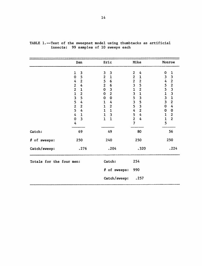
Thumbtack Test of the Model
A test of the model's validity was conducted using thumbtacks
as artificial insects. The advantage of thumbtacks over actual insects
was that the proportion in the path of the net (i.e. variable b) could
be fixed at 1.0 by properly placing the tacks on the plants. The test
designed to estimate the probability of getting into the net resulted
in 8 of 40 tacks being caught (i.e. p = 0.20). The four men used 12"
nets (i.e. d = 1.0) and took 5' sweeps (i.e. L = 5.0). In 18,000 square
feet there were 4867 tacks (i.e. D = 0.270). Substituting these
values into the model gives:
C = (1.0)(5.0)(0.270)(l.O)(O.20) = 0.270
Hence we expect (if the model is any good) that the four men should
average 0.270 thumbtacks per sweep. The actual catch (Table l) was
254 in 990 sweeps or 0.257 thumbtacks per sweep which is about 5%
different from the predicted.
14
TABLE 1.--Test of the sweepnet model using thumbtacks as artificial
insects: 99 samples of 10 sweeps each
Dan Eric Mike Monroe
1 3 3 3 2 4 O 1
O 5 2 1 2 1 3 3
4 2 5 6 2 2 4 2
2 4 2 6 3 5 5 2
2 l 0 3 1 2 5 3
1 2 0 2 3 1 l 3
3 5 O O 5 3 3 l
5 4 l 4 3 5 3 2
2 2 l 2 S 3 0 4
5 4 1 l 4 2 O 0
4 l l 3 5 4 l 2
0 3 l 1 2 4 l 2
4 7 5
Catch: 69 49 80 56
# of sweeps: 250 240 250 250
Catch/sweep: .276 .204 .320 .224
Totals for the four men: Catch: 254
# of sweeps: 990
Catch/sweep: .257

15
Vertical Distribution of the
Cereal Leaf Beetle
Vertical distributions were observed in wheat and oats in 1968.
The raw data is contained in the appendix and summarized in Figure 2.
Spring adults appear to move closer to the ground as wind speed increases.
At low wind speed a large majority were found in the top half of the
plants, while with 10 mph winds over 70% were in the lower half of the
plants. From zero to 28% of the beetles were found on the ground in-
stead of the plants, and this percentage appears unrelated to wind
speed. Larval distribution was bimodal in the one case observed. The
two peak heights correspond very closely to the heights of the top two
leaves of the host plant.
The four larval instars are not distributed the same on the
host plant. Table 2 shows that the smaller larvae are closer to the
ground than the larger ones. Sixty larvae of each instar were observed
on 38" wheat on June 5, 1968. The sky was clear, the temperature about
80°F, and the wind calm.
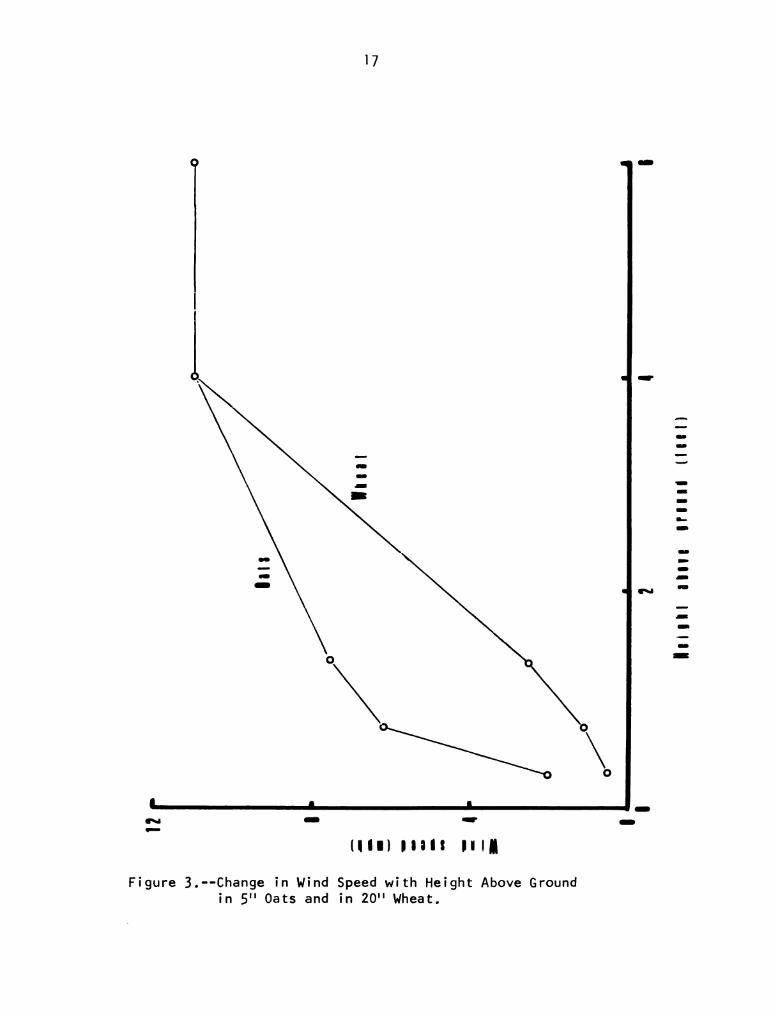
Wind Profile
Figure 3 shows the wind profile of May 16, 1968 at Galien,
Michigan. Each point plotted represents the mean of three values. In
both oats and wheat the wind speed at crOp height (5" and 20" respec-
tively) was 4.5 miles per hour compared with 11.4 mph at 6'6" above
the ground. The maximum height above the ground that beetles were found
in wheat was 12" and in oats 2". At these heights the wind speed was
1.6 miles per hour in both crops.

l6
IIII
IIII illl ll III
ll
Figure 2.--Six Cases of Cereal Leaf Beetle Vertical Distribution.
-
-
zN
O
O\
O
L J 1 fi-
N - _. -
(III) mu: In.
Figure 3.--Change in Wind Speed with Height Above Ground
in S” Oats and in 20” Wheat.
Illll
lfllll
llllll

18
TABLE 2.-—Difference in vertical distribution of the four larval
instars in 38" wheat
Instar
Vertical
location 1 2 3 4
Top
third 16 51 49 53
Middle
third 32 19 9 7
Bottom
third 12 O 2 0
Total
observed 60 60 60 6O
Converting Sweepnet Catch
to Absolute Density
Sweepnet catch is affected by several factors other than abso-
lute density. Solving equation (1) for density gives
_ 1
”-33:56 <2)
If M is defined as the "multiplication factor" required to convert
catch per sweep into density, then D = MC and from (2) above
1
M ' Dpr(3)
This usage of M is identical to that of Menhinick (1963). However,
his units were in meters while feet are used here.
In the results that follow all sweeping was done with 5' sweeps
of a 15" net. Using these values for L and d, a minimum theoretical
value for M can be calculated from (3) by using maximum possible values
for b and p.
l9
Mmin
= (1.25)<§)<1><1)
In practice the minimum observed value will be larger than this for two
reasons: it is unrealistic to assume that 100% of the insects will be
in the path of the sweepnet (Figure 2), and less than 100% of those in
the path will be caught in the net. In the following analysis the
maximum values of b and p were both taken as 0.90 resulting in
1
“min = (1.25)(5)(.9)(.9) = 0'
20
Sweepnet catch does not depend on whether sweeping is done with
or across the rows. In 300 sweeps the average catch per sweep across
rows was 1.67 compared to 1.64 with the rows (see Appendix for data).
The variances from the same data showed a six fold difference between
across and with row sweeping. The F test for variance homogeniety in-
dicates that the odds are 100 to 1 against these being the same.
Placement of the sampling cage did not significantly affect
sweepnet catch inside the cage. The 23 paired samples of 3 sweeps
each gave an average difference of -0.70 and a t value of -0.81, which
has a probability by random chance of over 20%. The raw data are in
the Appendix.
CrOp height, temperature, wind speed, relative humidity, and
intensity of solar radiation are the factors which were considered as
possibly affecting the multiplication factor M. The weather data used
were standard weather bureau measures and not microenvironmental in
nature. Table 3 lists the 15 data points used in the following multiple
regression analysis.
On any given sample date several estimates of catch per sweep
were made and likewise several estimates of absolute density. In

20
TABLE 3.—-Observed values of the multiplication factor M and the
associated physical conditions for adult cereal leaf beetles
Crap Temper- Wind Solar Relative
height ature speed radiation humidity M
40" 79°F 2 mph .9 40% .79i312
4O 75 3 .3 50 1.07:,31
4O 80 0 .9 45 .39:.20
24 80 0 .9 45 .35:.06
26 65 10 .9 35 1.09:.11
26 75 5 .7 50 .39:.15
26 85 0 1.1 40 .26:.03
26 85 2 1.1 40 .30:.OS
20 53 14 .3 85 1.21:,29
8 6O 5 .1 45 1.45:.37
9 68 10 1.1 35 .88:.18
12 55 2 .3 100 .47:,12
26 82 6 .4 81 .30:.11
20 86 6 1.0 68 .38:.05
26 86 8 .3 7O .57i.07
Solar radiation is measured in gram calories per square centi-
meter per minute.
The multiplication factor M is recorded plus or minus the
standard error.

21
general these were not paired. The mean and standard error of M were
obtained using the formula presented by Yates (1953).
Since the standard error of the estimates of M are quite variable,
the data was weighted by a factor of (SE)-2. This is recommended by
Draper and Smith (1966) and MAES (1967) as a means of placing proper
emphasis on those data points that contain the most accurate informa-
tion. The effect of this weighting is to consider each good point as
more than one observation and each sloppy point as less than one with
no net effect on the number of observations.
The analysis of the data on adult beetles in Table 3 went
through a number of iterations. The goal was a multiple regression
equation that gave a high multiple correlation coefficient without
requiring all five independent variables. A number of transformations
on each variable and several interaction terms were tried. However,
before going into these, it is necessary to introduce some notation:
H = plant height in inches
T = air temperature at 4 feet above ground in °F
W = wind speed at 6 feet above ground in miles per hour
RH = relative humidity at 4 feet above ground
S = solar radiation intensity in gram calories per square
centimeter per minute
M = multiplication factor
Transformed variables are denoted by subscripts (e.g. M1).
The following transformations were considered:
M = log10(M-0.20)
22 l
- log10(W + 1)
H1 = loglO(H)

22
T1 = T + 108
2
T2 - T
2
RH1 = RH
Each of these was based on logical considerations. Using M1 instead
of M would exclude the chance of predicting an M value less than 0.20,
which was previously shown to be impossible. Similarly W1 and H1
transformations would exclude the potential problem of considering
negative wind speeds and plant heights. Finally T was suggested as
1
an approximation to the internal temperature of the adult cereal leaf
beetle. Initially this was simply hypothesized on theoretical grounds,
but subsequently a thermocouple was inserted into a beetle which showed
a 10° F rise in temperature when the sun shown on the beetle. The
second power transformations of temperature and relative humidity were
considered on the assumption that some nonlinearily in these variables
may exist.
The regression equation chosen as being most practical is
M1 = -0.60 + .020H - .017T1 + .661W1
which has a multiple correlation coefficient of 4 = 0.934. The de-
tailed statistics are in Table 4. The equation is more useful when
the transformed variables are replaced with the proper expressions:
loglO(M-.20) = -.060+.020H-.Ol7(T+lOS)+.66l(log10(W+1))
Solving this for M gives:
M = 0.20 + 10(-.06O+.020H-.Ol7(T+lOS)+.66llog10(W+1))
Because of the difference in size and in vertical distribution
of the four larval instars, it was expected that the multiplication
factor M would be greater for small larvae than large ones. The

23
TABLE 4.--Statistics of the multiple regression for predicting M
Analysis of Variance
Source SS df MSS F
Total 1.8458 14 0.
Regression 1.6107 3 0.5369 25.13
Error 0.2351 11 0.0214
F = 25.13 is significant at .0005
Multiple correlation coefficient
r = .9342 r2 = .8727
Regression coefficients
Variable Coefficient F Significance
Constant -0.0599 1 .5034 0.014 .907
H 0.0198;t .0063 9.754 .010
T1 -0.0175;: .0049 12.838 .004
W1 0.66111: .1085 37.1358 .0005
Standard error of the estimate
SE = 0.1462

24
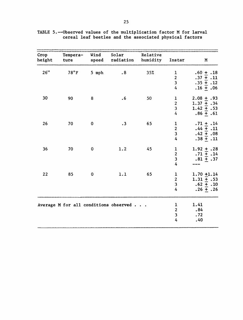
average M values from Table 5 were 1.41, 0.84, 0.72, and 0.40 for first
through fourth instar larvae respectively. These are averages from
five different situations where temperature ranged from 80°F to 90°F,
wind from calm to 8 mph, crop height from 22" to 36", and sky from over-
cast to clear. There was no observable relationship between M and_any
of the environmental parameters.
Components of Variance Involved in
Estimating Cereal Leaf Beetle Density
The sources of variation in any insect sampling plan designed
to estimate total population density in a region can be divided into
three categories. They are sampling error, within field variation, and
between field variation. The "field" designation may change from one
insect to another, but the idea stays the same. If the sampling is
done in a manner to satisfy the assumptions of a normal distribution,
then standard techniques are available to aid in the analysis.
Sampling error is presumed to be very small in relation to the
other two. Within field variance can be measured directly. Between
field variance could be measured directly only if every insect in each
field were counted. However, it is possible to directly measure a
component containing both within and between field variance. If this
component and the within field component are both accurately estimated,
then the between field variance can be arrived at by subtraction.
In any program of population sampling the variance ($2) at each
density is related to the mean (E). It is generally accepted that
sampling from a randomly distributed population will result in the
variance and the mean being equal. If the population is aggregated,
25
TABLE 5.--Observed values of the multiplication factor M for larval
cereal leaf beetles and the associated physical factors
Crop Tempera- Wind Solar Relative
height ture speed radiation humidity Instar M
26" 78°F 5 mph .8 35% 1 .60 :_.18
2 .37 :_.ll
3 .35 i_.12
4 .16 :_.06
3O 9O 8 .6 50 1 2.08 1;.93
2 1.37 i .34
3 1.42 11.53
4 .86 :_.61
26 70 0 .3 65 l .71 i .14
2 .44 i .11
3 .42 i .08
4 .38 :_.ll
36 70 0 1.2 45 l 1.92 i .28
2 .71 :_.14
3 .81 :_.37
4 __-
22 85 O 1.1 65 l 1.70 £1.14
2 1.31 i .53
3 .62 :_.10
4 .26 :_.26
Average M for all conditions observed . 1 1.41
2 .84
3 .72
4 .40

26
the variance will exceed the mean, while if the population is more uni-
formly distributed, the mean will exceed the variance.
Taylor (1961) presented the following equation to describe the
mathematical relationship between the variance and the mean:
32 = a<§)b
The factor a appears to be primarily a sampling and computing factor
while b appears to be a true population statistic related to aggrega-
tion. Taylor says b = 1 implies randomness.
Estimated values of a and b can be obtained from the regression
of log (82) on log (E). Finney (1941), Morris (1955), and Bliss (1967)
have shown that the arithmetic mean is under-estimated when predicted
from the regression equation of a logarithmic plot. Bliss suggested
A
that for the regression equation log y is desired:
? = 10(A-l-Blogx+l.1513EMSS)
where EMSS is the error mean sum of squares from the analysis of
variance table of the regression.
The above method of analysis was applied to the sweepnet catches.
Table 6 shows the regression statistics of the plots in Figure 4. The
raw data for the within field variance are recorded in Table 12 of the
Appendix. The between plus within field variance data were taken from
unpublished results of the Cooperative Cereal Leaf Beetle Survey
administered by Michigan State University. Within field variance (8:)
is related to mean catch per sample (E) by
s: = 0.90 EL“
and between plus within field variance (82 ) is related to the mean by
B+W
2 _ —1.9333+w — 1.77 x

27
TABLE 6.--Regression statistics for predicting within and between field
variances from mean catch per sample
Within Field
Source SS df MSS F
Total 20.698 19
Regression 20.326 1 20.326 984.4
Error .372 18 .021
a = -.0713 :_.0437 b = 1.4053 :_.0448
r = .991 r2 = .982
Significant at less than .0005
Between Field
Source SS df MSS F
Total 186.587 79
Regression 176.046 1 176.046 1302.6
Error 10.541 78 .135
a = .0930 :_.0826 b = 1.9336 1 .0536
r = .971 r2 = .944
Significant at less than .0005

'Iflllil
28
II'
o
mum
II‘ .o
o
o
0
"II
o
. 0 mm
.1 1 u III II" II
Illl Clltl lIr Slllll
Figure 4.--Relationship Between Mean Catch per Sweep and the Variance
Around that Mean for Within Field and Between Field Samples.

29
Using Taylor's criterion the cereal leaf beetle is slightly aggregated
within fields (b = 1.41) and more aggregated between fields (b = 1.93).
Between field variance is therefore described by the following equation:
2 _ 2 2 _ —1.93 _ —1.41SB — sB+w sW — 1.77x 0.90x
Table 7 was constructed from the three equations given above. It
shows that for all densities greater than one individual per sample the
between field variance exceeds within field variance. This information
will be analysed further in the discussion section to follow.
TABLE 7.--Within and between field variance as predicted from the
regression equations
__ Within Between Within +
x Statistic Fields Fields Between
2.1 s .035 -.015 .021
cv 187 -121 143
1. $2 .90 .87 1.77
cv 95 93 133
10. 32 23. 129. 152.
cv 48 114 123
100. s2 580. 12,480. 13,060.
cv 24 112 114
1000. $2 15,000. 1,106,000. 1,121,000.
cv 12 105 106
10000. s2 370,000. 95,830,000. 96,200,000.
cv 6 98 98
;'= mean catch per sample.
2
s variance about the mean.
CV s/x'= coefficient of variation.

DISCUSSION
Mathematical Model
One excellent characteristic of the proposed mathematical model
is its generality. It is not restricted to one life stage, nor in fact
to the cereal leaf beetle. Conclusions drawn from analysis of the model
will apply to any life stage of any insect in any crop. In fact the
model applies to sampling with a dip net in a pond or with a beating
net in brush.
It was shown earlier that if the net size and length of each
sweep are standardized, then the multiplication factor (M) is propor—
tional to (bp)—1 where b is the proportion of the insect population that
is in the net's path and p is the probability of capture given that the
insect is in the net's path. Submodels for b and p could be developed.
However these would lack the generality of the main model. For the
cereal leaf beetle these could probably be submodeled in terms of wind,
temperature, and plant height. Most likely separate submodels would be
required for each life stage.
The factor b is affected by the sweepnet diameter, the height
above the ground that the sweepnet rim is moving, and the insects
vertical distribution in the host crOp. Consider as an example a
hypothetical case where all of the insects are at 5 inches above the
ground (say in a 10 inch tall host crop), and the sweepnet Operator
3O


31
sweeps with the rim of the 15" net just two inches above the ground.
Then at 5 inches, because the net opening is not square, somewhat less
than the full 15" is being swept. Actually about 80% of that width is
being swept, hence b = 0.80.
As a second example say all of the insects were at 9.5 inches
with other conditions as above. Since this is the height of the net
center, 100% of the population is in the net's path, hence b = 1.00.
Thirdly consider a case where two thirds are at 5" and one third
at 9.5 inches. Then b is found as follows
1):
COIN
(0.80) +% (1.00) = 0.87
Following the above procedure and applying it to the Observed
vertical distributions in Figure 2, it was possible to compute b values
for several assumed heights of sweeping. Table 8 gives the results,
from which we see that there is an Optimal height at which to sweep,
but that in most cases the difference of a few inches makes little or
no difference in b. The optimal height to sweep appears to be with
the top edge of the net two to four inches below the tOp of the plant.
Although no samples were taken in headed grain, it would seem that the
net should be used there as if the top leaves were the tap of the plant
since the beetle is very seldom seen on the head.
Final development of this model requires submodeling the factor
p. This was not attempted here as no method was devised to accurately
measure the value of p.
Regression Model
The regression model selected was one of many possible choices.
It was chosen because it accounts for a large percentage of the

32
TABLE 8.--Computed values for the factor b for various heights of the
sweepnet rim above the ground, and for the particular vertical
distributions shown in Figure 2
Vertical Distribution Height of Rim Computed Value
as Shown in Above Ground for b
Figure 2a 0" .69
l .66
2 .60
3 .54
4 .44
Figure 2b 0" .63
l .54
2 .46
3 .29
4 .19
Figure 2c 0" .70
1 .56
2 .43
3 .31
4 .16
Figure 2d 12" .47
14 .48
16 .52
18 .55
20 .51
22 .42
24 .33
Figure 2e 2" .77
4 .85
6 .85
8 .82
10 .68
Figure 2f 2" .67
4 .55
6 .34
8 .16
10 .05

33
variation in M and at the same time does not contain a large number of
independent variables. The latter is desirable in order to both simplify
computations when using the model and reduce the effort needed to col-
lect data for the model's use.
There are statistical considerations that should not be over-
looked in selection of a regression equation. The figures in Table 4
were computed as if this regression were the only one considered.
Furnival (1964) emphasizes that "practically every statistic computed
for the equation or equations developed through the screening process
is biased". He also states that practically nothing is known about the
magnitude of the biases, but their directions are known. Regression
coefficients are overestimated, while the standard error of the coeffi—
cients and the multiple correlation coefficient are underestimated.
One result is that all F statistics are overestimated, hence the levels
of significance are biased toward rejection of the null hypothesis.
The fact that these biases exist should not be cause for re-
jection of the equation nor for rejection of selecting a "best" re-
gression equation. Instead it should serve as a warning that the pre-
dicted values of‘M from this equation may not be as accurate as the r2
indicated. Further data collection would easily establish better
estimates of all coefficients and probabilities.
Comparing the Two Models
Two quite different models have been discussed. Neither one is
complete by itself, but when used together they allow a better under-
standing of the factors affecting sweepnet catch.

34
The mathematical model, in its generality, was unable to provide
numerical information for converting sweepnet catch into number per
unit area. However, it did provide a minimum theoretical value that
the multiplication factor (M) could assume. It also pointed out en-
vironmental factors likely to affect M through the factors b and p.1
Vertical distribution clearly affects b. Vertical distribution in turn
is affected by wind and crop height. Other factors presumed to affect
vertical distribution via the insects behavior were temperature, rela~
tive humidity, and solar radiation. It was also clear that these
factors would affect adults different from larvae. Factor p was, and
remains, less understood. It may indeed be a constant.
The regression equation used this information to predict M from
the environmental factors. This expression for M was then substituted
into the mathematical model to give the final result
D = (O 20 + 10-0.06+.020H-.017(T+1OS)+.66log(W+l))C
This equation applies only to the Special case for which the regression
model was developed.
Vertical Distribution
The proportion of the insect population that is in the sweepnets
path (b) is primarily affected by the insects vertical distribution.
Since the other parameters in the mathematical model (i.e. the factors
d, L, and p) are considered to be less variable than b, it is evident
that vertical distribution is the most important biological phenomenon
affecting the multiplication factor M. A good submodel for vertical
1Recall that b is the prOportion of insects in the sweepnets
path and p is the probability of capture for the proportion.

35
distribution would therefore greatly improve the usefulness of the
proposed mathematical model.
It has been shown here that wind is an important factor in adult
distribution. Although no mathematical description of its affect is
hypothesized, it appears that the beetle seeks microhabitats where the
wind speed is below 1.6 miles per hour. The relationship between wind
and larval distribution was not considered.
It was observed that first instar larvae are distributed closer
to the ground than are the other instars. This is probably a conse-
quence of plant growth during the time between oviposition and egg
hatch. Even if an egg were laid on the top most leaf of a young plant,
by the time that egg hatched there would be one or two leaves above
the first. Hence first instar larvae cannot appear in the top portion
of a plant unless they walk up there. Small larvae do less walking
than the larger ones, hence are less frequently found in the tOp part
of the plant.
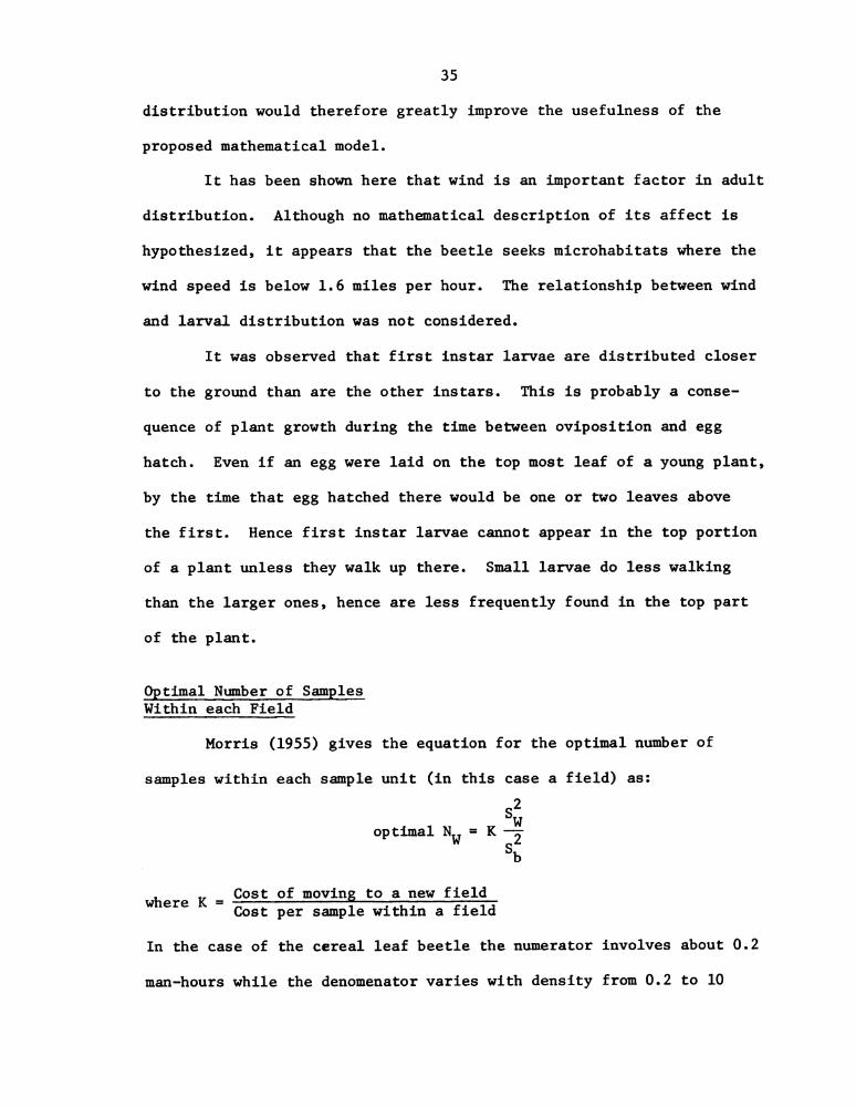
Optimal Number of Samples
Within each Field
Morris (1955) gives the equation for the Optimal number of
samples within each sample unit (in this case a field) as:
optimal Nw = K
65%|
2‘”...
Cost of moving to a new field
Cost per sample within a field
where K =
In the case of the cereal leaf beetle the numerator involves about 0.2
man-hours while the denomenator varies with density from 0.2 to 10


36
man-hours. The largest value K can assume is therefore 1.0, which occurs
at low densities. The ratio of within field variance to between field
variance also varies with density and takes on a maximum value of
about 1.0 at a density of one beetle per sample.1 Substituting these
maximum values into the above equation shows that the Optimum number
of samples within a field cannot exceed one. Hence the ideal plan
within each field is to take one sample and catch one cereal leaf
beetle; in other words sample until one beetle is caught.
Optimal Number of Fields per Township
The number of fields to sample per township, unlike the number
of samples within each field, depends on the accuracy required of the
estimated mean. In population sampling it is common practice to express
accuracy as the ratio of the standard error to the mean. Using this
approach together with the relationship between mean catch per sample
and variance, an equation relating accuracy to number of fields sampled
is obtained.
The following algebraic notation is needed:
;'= mean catch per sample
SE standard error of the catch per sample
a = accuracy, defined as SE/x
s = variance of the catch per sample
NF = total number of fields in the township containing the
crop being sampled
n = the number of those NF fields which are sampled
1It is assumed that a sampling scheme which yields a mean of
less than one beetle per sample is unacceptable because all the sta—
tistics used in this thesis assume a normally distributed population.
A large number of zeros in the data would violate this assumption and
hence invalidate the statistics.

Illlllilllulullllsll'
ill
AIIIrIII-{1'1
'1I'll
‘

37
Wadley (1967) gives the formula
2 l 1
SE - S (n - NF)
as being the proper relationship between standard error and variance
when n is greater than 10% of NF. When the sampling universe is re-
stricted to one township, this is a necessary consideration. Since
a = SE/x, the expression a E may be substituted into the above formula
for SE to give
szNF
s2+a2xNF
n:
when solved for n. In the case of the cereal leaf beetle the equation
can be further simplified by the approximation
32 = 1.77322
Although the true expression for this variance is 1.77§1°93, the approxi-
mation is justifiable. In Table 6 the standard error of the exponent
1.93 is given as 0.05, and therefore the t test value is 0.07/0.05 = 1.4
(for testing the hypothesis that the exponent is 2.00) which has a
probability between 10% and 20% by pure chance.
Substitution of 32 = 1.77§2 into the above expression for n
yields (after cancelling R):
n = 1.77NF
1.77+a2NF
Table 9 follows directly from this equation. Assuming the number of
fields in the township is known, one can either find the standard error
of the estimated mean from the number of fields sampled or the number
of fields to sample if a certain level of accuracy is desired. In
southern Michigan an average township may have between 50 and 200 oat

38
fields, hence if an accuracy of :_10% was required, about 60% of the
fields should be sampled.
TABLE 9.-—Predicted number of fields to sample for certain values of
NF and a
a
NF 5% 10% 20% 50% 100%
20 20 18 14 6 2
50 47 39 24 7 2
100 88 64 31 7 2
200 156 94 37 7 2
500 293 131 41 7 2
Exceptional Cases
All statistics calculated in the previous sections assumed (and
therefore apply only to) a so called "normal situation". In the real
world abnormal situations are actually rather common, and it is up to
the man in the field to recognize these and act accordingly. Within
field variance may be much increased over the normal in any of the
following ways:
1. Insecticide drift.
Figure 5 shows that in the parts Of the oat field where the
apple spray had drifted in from the orchard, the beetle
population was completely killed. In other parts of the
field the population was quite normal.

39
IIIII
Iftllfl
Figure 5.--Catch per l00 Sweeps in Ten Regions of an Oat Field
Adjacent to an Apple Orchard.
l
l
I.
II?
5|
8IIII!
IIII Islslli lll lelslly
IIII
5|
-_____——
o.
-
-
-
-
o.
-
a
h
-
-
all
n
Figure 6.--Catch per 50 Sweeps Along Three Transects in Wheat
Adjacent to Oats (Spring Adults).

40
P0pulation overflow.
Figure 6 shows how the proximity of a more favorable host crOp
can affect the population distribution in another host crOp.
In this case the density in the oats was Over 20 times that
in the wheat. The border of the wheat adjacent to the oats
held a pOpulation about seven times greater than the field as
a whole.
. HeterOgeneous stand of the host crOp.
When the condition of the host crOp is highly variable, the
beetle distribution within that crOp may also be highly
variable. Examples of host crOp heterogeniety are: l) weedy
patches 2) spots of thin stand 3) uneven maturity 3) un-
even crop height.
CONCLUSIONS
Sweepnet catch is related to density by the following mathematical
model:
__C_
D ’ dpr
This model applies to any insect in any crOp, but is of limited appli-
cability unless the parameters b and p are submodeled. The parameter b
is principally affected by the insect's vertical distribution which in
turn is affected by wind speed. No work was done on submodeling p.
An alternate method of relating sweepnet catch to density is
through the use of multiple regression statistics. The following equa-
tion predicts the value of M for adult cereal leaf beetles:
M = .20 + 10(-.06 + .020H - .017(T+lOS) + .66log(W+l))
Multiplication of catch per sweep by M will give number per square foot.
This regression has an r2 of 0.87 which leaves only 13% of the varia-
tion unaccounted for. No regression equation is developed for larvae,
but it is shown that M is inversely related to larval size.
The variance between samples within a field is related to the
mean of those samples by the equation:
52 = 0.897ml'405
while the combined between-within field variance is related to the
corresponding mean by:
s2 = 1.772ml°934
41

42
Hence at high densities the between field variance is much greater than
within field variance, while at densities near one individual per sample
the two components are nearly equal. A mean below one per sample
should be avoided since many zeros in any data requires special sta-
tistical treatment.
Optimal allocation of sampling resources in a cereal leaf beetle
survey requires one sample per field and as many fields per township
as is possible with those resources. Normally if 60% of the fields of
one crop are sampled, then for that crOp the standard error of the
catch per sample is within 10% of the mean.

LITERATURE CITED

LITERATURE CITED
Banks, C. J. and Brown, E. S. 1962. A comparison of methods of esti-
mating population density Of adult summ pest, Eurygaster
integriceps Put. (Hemiptera, Scutelleridae) in wheat fields.
Ent. Exp. and Appl. 5:255-260.
Beall, G. 1935. Study of arthropod populations by the method of
sweeping. Ecology 16(2):216-225.
Bliss, C. I. 1967. Statistics in biology, volume 1. McGraw-Hill
Book Co., New York. 558 pp.
Bremi-Wolf, J. J. 1846. Beitrag zur Kenntiuss der Dipteren,
insbesondere iiber das Vorkommen mehrerer Gattungen nach
besonderen Localitaten und die Fang derselben, so wei anch
iiber die Lebensweise lineger Larven. Isis III: p. 164-175.
Castro, T. R., Ruppel, R. F., and Gomulinski, M. S. 1965. Natural
history of the cereal leaf beetle in Michigan. Mich. Agr.
Expt. Sta. Quart. Bull. 47(4):623-653.
DeLong, D. M. 1932. Some problems encountered in the estimation of
insect populations by the sweeping method. Ann. Ent. Soc. Am.
25:13-17.
Draper, N. R. and Smith, H. 1966. Applied regression analysis,
New York, Wiley. 407 pp.
Finney, D. J. 1941. On the distribution of a variate whose logarithm
is normally distributed. J. Roy. Stat. Soc. Suppl. 7:155-161.
Furnival, G. M. 1964. More on the elusive formula of best fit. Proc.
Soc. of Am. For. pp. 201-207.
Gray, H. E. and Treloar, A. E. 1933. On the enumeration of insect
pOpulations by the method of net collection. Ecology 14(4):
356-367.
Gray, H. E. and Treloar, A. E. 1935. Note on the enumeration of
insect populations by the method of net collection. Ecology
16(1):122.
43

44
Helgesen, R. G. 1969. The within generation population dynamics of
the cereal leaf beetle, Oulema melanopus (L.) Ph.D. thesis,
Michigan State University. 96 pp.
Hughes, R. D. 1955. The influence of the prevailing weather on the
numbers of Meromyza variegata Meigen (Diptera, ChlorOpidae)
caught with a sweepnet. J. Anim. Ecol. 24:324-342.
Menhinick, E. F. 1963. Estimation of insect population density in
herbaceous vegation with emphasis on removal sweeping. Ecology
44(3):617-621.
Michigan Agricultural Experiment Station. 1967. Weighting of obser-
vations in least squares problems (weighted regression) and in
calculating basic statistics (LS routine). STAT series
description no. 12. Agricultural Experiment Station, Michigan
State University. 5 pp.
Morris, R. F. 1955. The development of sampling techniques for
forest insect defoliators, with particular reference to the
spruce budworm. Can. J. 2001. 33:225-294.
Morris, R. F. 1960. Sampling insect populations. Ann. Rev. Entomol.
Romney, V. E. 1945. The effect of physical factors upon catch of
the beet leafhopper (Euteltia tenellus (Bak.)) by a cylinder
and two sweepnet methods. Ecology 26(2):135-147.
Ruppel, R. F. 1964. Biology of the cereal leaf beetle. Ent. Soc.
Amer. N. Cent. Br. Proc. 19:122-124.
Shade, R. E. and Wilson, M. C. 1964. Population buildup of the
cereal leaf beetle and the apparent influence of wind on dis-
persion. Research Progress Report 98, Purdue Univ. Agr. Expt.
Stat., Lafayette, Indiana.
Southwood, T. R. E. 1966. Ecological methods with particular refer-
ence to the study of insect populations. London, Methuen,
pp. 189-191.
Taylor, L. R. 1961. Aggregation, variance and the mean. Nature
189:732-735.
U.S. Department of Agriculture. Cooperative Economic Insect Report,
19(28):534, 1969.
Wadley, F. M. 1967. Experimental Statistics in entomology. Graduate
School Press U.S.D.A., Washington, D.C.

45
Yates, F. 1953. Sampling methods for censuses and surveys, 2nd ed.,
London, Griffin. 401 pp.
Yun, Y. M. 1967. Effects of some physical and biological factors on
the reproduction, development, survival, and behavior of the
cereal leaf beetle, Oulema melanopus (L.), under laboratory
conditions. Ph.D. thesis, Michigan State University. 153 pp.

APPENDIX

46
TABLE 10.--Grain row direction in relation to sweeping direction as it
affects sweepnet catch of spring adults
Sweeping With Sweeping Across
the Rows the Rows
10 17
13 17
17 11
17 13
12 22
17 12
18 25
18 9
25 22
16 14
15 6
13 13
17 13
18 4O
17
20
Mean 16.4 16.7
Variance 12.1 72.7

47
TABLE ll.--Comparison of sweepnet catch of summer adults inside and
outside of sampling cage
Inside Outside
OOHOl-‘ONl-‘OCD-L‘Nl-‘l-‘OO‘O‘NkON
1.1
ONOI—‘ONCl—‘OCfiO‘QWO‘WO‘DO‘O‘O
Sum 171 187
94
0.696
t 0.806 with 22 degrees of freedom

48
TABLE 12.--Within field variation in sweepnet catch
Information regarding date, host, life stage sampled, and number
of sweeps per sample is followed by the actual catches in the order
taken.
1. April 22, wheat, adults, 3 sweeps/sample:
0,2,1,l,3,3,2,3,3,3,6,5,3,3,3,0,2,0,0,0,5,1,1.
2. April 22, wheat, adults, 3 sweeps/sample: !
0,3,2,0,2,3,11,1,1,5,6,2,1,3,2,3,6,3,4,3,2,1,3.
3. April 22, wheat, adults, 3 sweeps/sample:
0,0,0,l,0,3,0,0,3,1,0,l,l,0,0,0,0,0,l,1,0,2,0.
4. April 23, wheat, adults, 10 sweeps/sample:
17,17,11,13,22,12,25,9,22,14,6,13,13,40,25,16,15,13,17,18,
17,20,10,l3,17,17,12,l7,18,18.
5. May 7, wheat, adults, 3 sweeps/sample:
1,0,1,1,0,0,0,1,1,0,0,l,l,0,1,0,0,0,0,0,0,0,0.
6. May 24, wheat, adults, 3 sweeps/sample:
14,13,l,ll,7,8,13,7,ll,15,18,11,15,4,9,10,7,9,4,11.
7. May 24, oats, adults, 10 sweeps/sample:
5,l,5,6,13,4,12,11,13,17,5,11,21,10,13,10,10,8,4,5.
8. July 2, oats, larvae, 10 sweeps/sample:
1,1,1,4,1,1,2,1,2,1,1,3,2,2,0,0,1,1,1,2,1,4,2,2,2,4,1,1.
9. July 3, oats, larvae, lO sweeps/sample:
2,3,3,0,2,0,0,l,0,1,0,l,1,0,0,1,2,2,0,2,0,1,3,3,2,1.
10. July 3, oats, larvae, 10 sweeps/sample:
1,0,0,1,2,l,l,2,1,2,2,l,0,1,1,1,1,2,2,3,0,2,l,2,2,3.
11. July 3, oats, adults, 10 sweeps/sample:
1,0,0,1,0,0,0,l,2,0,2,2,2,2,0,0,0,0,0,0,0,0,0,0,0,l.
12. July 3, oats, adults, 10 sweeps/sample:
O,1,0,0,0,l,0,0,0,0,1,0,0,0,0,0,0,0,1,0,0,0,1,0,1,0.
13. July 5, barley, larvae, 3 sweeps/sample:
5,2,2,1,3,7,2,1,2,3,3,3,3,4,3,3,1,2,2,3,2,7,2,1,l,5,8,4,5,
2,2,3,0,6,2,4,0,0,4,3,4,4,2,2,2,3,l,2,3,3,2,l,0,5,0,7,5,0,
l,3,6,4,3,0.

49
Table 12 (cont'd.)
14.
15.
16.
17.
18.
19.
20.
21.
22.
July 5, barley, larvae, 3 sweeps/sample:
2,3,3,2,4,0,3,3,0,0,0,2,2,0,0,3,1,1,4,0,3,0,2,0,1,0,0,2,1,3,
l,l,0,0,l,2,2,1,0,0,4,2,5,2,3,1,l,l,2,0,0,2,1,2,0,3,l,2,2,3,
5,2,0,5.
July 7, corn, adults, 10 sweeps/sample:
32,45,35,33,29,44,23,28,36,27,34,48,40,32,35,23,47,37,18,23.
July 9, wheat, adult
2,4,3,0,1,l,l,1,0
HOG)
1,3,1,1,l,0,0,1,2,
2.l-‘
U
DJ
U
l-'
U
l-‘
U
.l.\
U
N H
U
Do
U
[.1
UU
\INCD
uvo
MUD
v
I-‘C‘Da
July 18, oats, adults, 3 sweeps/sample:
11,6,17,11,5,5,14,15,14,8,5,l,5,9,5,7,11,6,9,9.
July 18, oats, adults, 3 sweeps/sample:
4,2,2,4,2,2,7,7,9,7,6,7,8,2,l,4,5,l,2,7.
May 23, barley, adults, 30 sweeps/sample:
123,78,99,66,134,136.
May 23, barley, adults, 50 sweeps/sample:
255,375,400,289,419,353.

”TllllllllfllfllllMilli)llllllll'es