240 Chapter 4. Theoretical Foundation and Background Material: Modeling of Dynamic Systems

io(t) = engine speed

a(i) = throttle position

Xo = time delay in engine

Je — inertia of engine

The following assumptions and mathematical relations between the engine variables are given:

1. The rate of air flow into the manifold is linearly dependent on the throttle position:

dqi(t)

dt — K\a{t) K\ = proportional constant

2. The rate of air flow leaving the manifold depends linearly on the air mass in the manifold and the engine speed:

dt = K2qm(t) + Ksco(t) K2, K?, = constant

3. A pure time delay of r© seconds exists between the change in the manifold air mass and the engine torque:

T(t) = K*qm{t — T£>) A4 = constant

4. The engine drag is modeled by a viscous-friction torque Bco(t), where B is the viscous-friction coefficient.

5. The average air mass qm{t) is determined from

'dqi(t) dq0{tf qm{t) = J dt dt dt

6. The equation describing the mechanical components is

T(t)=J^ + Ba>(t) + Td

(a) Draw a functional block diagram of the system with a (t) as the input, co(t) as the output, and Tcl as the disturbance input. Show the transfer function of each block.

(b) Find the transfer function Cl(s)/a(s) of the system.

(c) Find the characteristic equation and show that it is not rational with constant coefficients.

(d) Approximate the engine time delay by

. - ^ 1 - ^ / 2 1 + zDs/2

and repeat parts (b) and (c). 4-37. Vibration can also be exhibited in fluid systems. Fig. 4P-37 shows a U tube manometer.

ft y(t)

Figure 4P-37

Assume the length of fluid is L, the weight density is /x, and the cross-section area of the tube is A. (a) Write the state equation of the system.

(b) Calculate the natural frequency of oscillation of the fluid.

4-38. A long pipeline connects a water reservoir to a hydraulic generator system as shown in Fig. 4P-38.

Problems 241

Q,v. P,A

Q.v

Figure 4P-38

At the end of the pipeline, there is a valve controlled by a speed controller. It may be closed quickly to stop the water flow if the generator loses its load. Determine the dynamic model for the level of the surge tank. Consider the turbine-generator is an energy converter. Assign any required parameters.

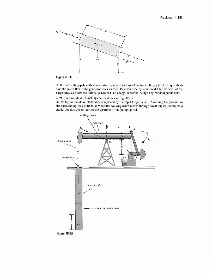
4-39. A simplified oil well system is shown in Fig. 4P-39. In this figure, the drive machinery is replaced by the input torque, 7),,(/)- Assuming the pressure in the surrounding rock is fixed at P and the walking beam moves through small angles, determine a model for this system during the upstroke of the pumping rod.

Walking Beam

Flexible Rod

No friction

T h

1 Figure 4P-39

Sucker rod

Internal radius = R

Chapter 4. Theoretical Foundation and Background Material: Modeling of Dynamic Systems

4-40. A hydraulic servomotor usually is used for the speed control of engines. As shown in Fig. 4P-40, the reference speed is controlled by the throttle lever. The flyweight is moved by engine, so then the differential displacement of the spring determines the input to the hydraulic servomotor. Determine the state space model of the system.

Figure 4P-40

4-41. Fig. 4P-41 shows a two-tank liquid-level system. Assume that Qj and Q2 are the steady-state inflow rates, and H, and H2 are steady-state heads. If the other quantities shown in Fig. 4P-41 are supposed to be small, derive the state-space model of the system when h/ and h2 are outputs of the system and qi} and qi2 are the inputs.

HM

X ^ • Q i+*2-Nfo

fil-h?!

Figure 4P-41

PROBLEMS FOR SECTION 4-6 4-42. An accelerometer is a transducer as shown in Fig. 4P-42. (a) Find the dynamic equation of motion.

(b) Determine the transfer function.

(c) Use MATLAB to plot its impulse response.

Problems 243

Figure 4P-42

4-43. Fig. 4P-43(a) shows the setup of the temperature control of an air-flow system. The hot-water reservoir supplies (he water that flows into the heat exchanger for heating the air. The temperature sensor senses the air temperature TAO and sends it to be compared with the reference temperature Tr.

HOT-WATER RESERVOIR

Valve 53-1

/ F a n MA

w„

Pit)

ELECTRIC-TO-PNEUMATIC

TRANSDUCER

«W

CONTROLLER

Air intake Heat exchanger

Temperature sensor F.

+. Heated air

(a)

r, /-+ v .

_ i y Error

r

CONTROLLER — •

ELECTRIC-TO-PNEUMATIC

TRANSDUCER

y;

Pit) Ik P

PNEUMATIC ACTUATOR/VALVE

TEMPERATURE SEr-JSOR

dMw

• HEAT

EXCHANGER

4 .

^

Output air

temperature TAo

r

(b)

Figure 4P-43

244 Chapter 4. Theoretical Foundation and Background Material: Modeling of Dynamic Systems

The temperature error Te is sent to the controller, which has the transfer function Gc(s). The output of the controller, u{t), which is an electric signal, is converted to a pneumatic signal by a transducer. The output of the actuator controls the water-flow rate through the three-way valve. Fig. 4P-43(b) shows the block diagram of the system.

The following parameters and variables are defined: dMw is the flow rate of the heating fluid = KMu; KM = 0.054 kg/s/V; 7",,, the water temperature = KRdMw; KR = 65°C/kg/s; and TAO, the output air temperature. Heat-transfer equation between water and air:

dTA0

dt = Tw — TAO *C = 10 seconds

Temperature sensor equation:

dTs _ T„v — j - = TAO - Ts dt

X, — 2 seconds

(a) Draw a functional block diagram that includes all the transfer functions of the system.

(b) Derive the transfer function TAo(s)/Tr(s) when Gc(s) = 1.

4-44. An open-loop motor control system is shown in Fig. 4P-44.

Potentiometer

0,,,« K 0L(t) Ev.

Figure 4P-44

The potentiometer has a maximum range of 10 turns (20jrrad). Find the transfer functions E„(s)/

Tm(s). The following parameters and variables are defined: 9„,(t) is the motor displacement; 9i(t),

the load displacement; Tm{t), the motor torque; J,„, the motor inertia; B„„ the motor viscous-friction coefficient; Bp, the potentiometer viscous-friction coefficient; e0(t), the output voltage; and K, the torsional spring constant.

4-45. The schematic diagram of a control system containing a motor coupled to a tachometer and an inertial load is shown in Fig. 4P-45. The following parameters and variables are defined: Tm is the motor torque; /„„ the motor inertia; J„ the tachometer inertia; JL, the load inertia; Kx and K2, the spring constants of the shafts; 9,, the tachometer displacement; 0nl, the motor velocity; 9L, the load displacement; to,, the tachometer velocity; COL, the load velocity; andB„„ the motor viscous-friction coefficient.

(a) Write the state equations of the system using 9L, O>L, 0,, co,, 9m, and<ura as the state variables (in the listed order). The motor torque 7),, is the input.

(b) Draw a signal flow diagram with Tm at the left and ending with 9^ on the far right. The state

diagram should have a total of 10 nodes. Leave out the initial states.

/ M J -A ,K P „ " , F f •• ®L(S) &,(S) 0,,,(4-) (c) Find the following transfer functions: _ . . — — _ , .

Tm{s) Tm(s) Tm(s) (d) Find the characteristic equation of the system.

9,,,- co„ *»«*» ei.

J, \ KX \

I I •/,„ 1 Kl \

jr r̂ h

Tachometer

Figure 4P-45

Motor Load

Problems 245

4-46. Phase-locked loops are control systems used for precision motor-speed control. The basic elements of a phase-locked loop system incorporating a dc motor are shown in Fig. 4P-46(a). An input pulse train represents the reference frequency or desired output speed. The digital encoder produces digital pulses that represent motor speed. The phase detector compares the motor speed and the reference frequency and sends an error voltage to the filter (controller) that governs the dynamic response of the system. Phase detector gain = Kp, encoder gain = Kc, counter gain = 1 /TV, and dc-motor torque constant = K/. Assume zero inductance and zero friction for the motor.

(a) Derive the transfer function Ec(s)/E(s) of the filter shown in Fig. 4P-46(b). Assume that the filter sees infinite impedance at the output and zero impedance at the input.

(b) Draw a functional block diagram of the system with gains or transfer functions in the blocks.

(c) Derive the forward-path transfer function llllt(s)/E(s) when the feedback path is open.

(d) Find the closed-loop transfer function ilm(s)/Fr(s).

(e) Repeat parts (a), (c), and (d) for the filter shown in Fig. 4P-46(c).

(f) The digital encoder has an output of 36 pulses per revolution. The reference frequency fr is fixed at 120 pulses/s. Find Ke in pulses/rad. The idea of using the counter N is that, with/,, fixed, various desired output speeds can be attained by changing the value olN. Find N if the desired output speed is 200 rpm. Find N if the desired output speed is 1800 rpm.

Reference frequency

PHASE DETECTOR

e(t)

Error voltage

FILTER ec(t)

COUNTER Feedback

pulses

AMPLIFIER K

dc motor

Wv—

Ke

DIGITAL ENCODER

} LOAD

h

(a)

e{t)

(b)

Figure 4P-46

Rn C

(c)

er(t)

4-47. Describe how an incremental encoder can be used as a frequency divider.

PROBLEMS FOR SECTION 4-7 4-48. The voltage equation of a dc motor is written as

ea(t) = Raia(t) + La^jf- + Kbcom{t)

where eu{t) is the applied voltage; ia(t), the armature current; Rtl, the armature resistance; La, the

armature inductance; AT/,, the back-emf constant; co,„(t), the motor velocity; and con[t), the reference

input voltage. Taking the Laplace transform on both sides of the voltage equation, with zero initial

246 Chapter 4. Theoretical Foundation and Background Material: Modeling of Dynamic Systems

conditions and solving for £lm(s), we get

nm(s) = Eg(s) - (Rg + LgS)Ia(s)

which shows that the velocity information can be generated by feeding back the armature voltage and current. The block diagram in Fig. 4P-48 shows a dc-motor system, with voltage and current feedbacks, for speed control. (a) Let K] be a very high gain amplifier. Show that when H((s)/He(s) = —(/?<, + Las), the motor velocity com(t) is totally independent of the load-disturbance torque TL.

(b) Find the transfer function between £lm (s) and Or(j)(7t = 0) when H,{s) and Hc,(s) are selected as in part (a).

"Sf^i ~Y~~

1

Volu

*,

He(s)

nop fppH

tf,-uv

e / N

+ \^S

r

harW

Figure 4P-48 ^

Current feedback

1 K + Lj

lL

i *«

K*

Motor an

1 Yu ^AJ^ 4

d Initd

i B + Js

a)

h. W

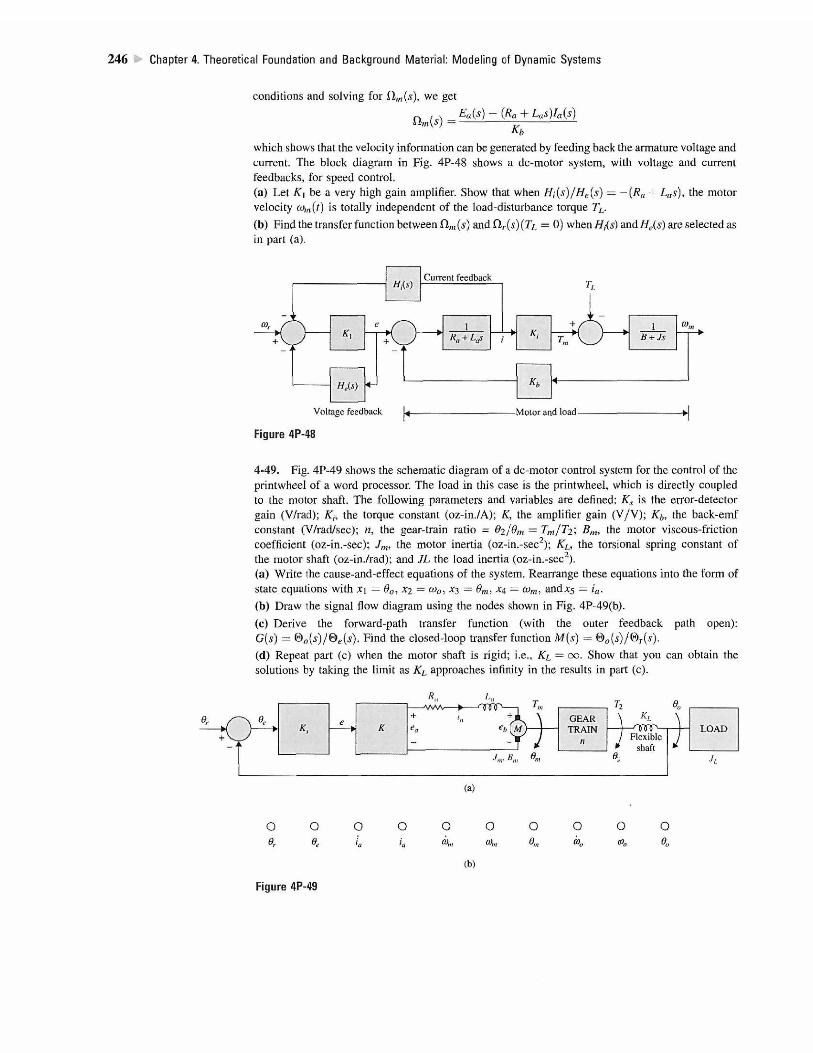
4-49. Fig. 4P-49 shows the schematic diagram of a dc-motor control system for the control of the printwheel of a word processor. The load in this case is the printwheel, which is directly coupled to the motor shaft. The following parameters and variables are defined: Ks is the error-detector gain (V/rad); K/, the torque constant (oz-in./A); K, the amplifier gain (V/V); K/„ the back-emf constant (V/rad/sec); n, the gear-train ratio = QijOm = Tm/T2', Bm, the motor viscous-friction coefficient (oz-in.-sec); /,„, the motor inertia (oz-in.-sec2); KL, the torsional spring constant of the motor shaft (oz-in./rad); and JL the load inertia (oz-in.-sec2). (a) Write the cause-and-effect equations of the system. Rearrange these equations into the form of state equations with xi = 60, xi = co0, *3 = 0m, X4 = com, and^5 = ia.

(b) Draw the signal flow diagram using the nodes shown in Fig. 4P-49(b).

(c) Derive the forward-path transfer function (with the outer feedback path open): G(s) = &0(s)/®e(s). Find the closed-loop transfer function M(s) = <d0(s)/®T(s).

(d) Repeat part (c) when the motor shaft is rigid; i.e., KL = 00. Show that you can obtain the solutions by taking the limit as KL approaches infinity in the results in part (c).

** GEAR TRAIN

Flexible * shaft ft

LOAD

(a)

O O O O O O O O o 0

(b)

Figure 4P-49

Problems 247

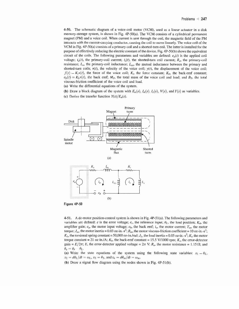
4-50. The schematic diagram of a voice-coil motor (VCM), used as a linear actuator in a disk memory-storage system, is shown in Fig. 4P-50(a). The VCM consists of a cylindrical permanent magnet (PM) and a voice coil. When current is sent through the coil, the magnetic field of the PM interacts with the current-carrying conductor, causing the coil to move linearly. The voice coil of the VCM in Fig. 4P-50(a) consists of a primary coil and a shorted-turn coil. The latter is installed for the purpose of effectively reducing the electric constant of the device. Fig. 4P-50(b) shows the equivalent circuit of the coils. The following parameters and variables are denned: ea(t) is the applied coil voltage; ia(t), the primary-coil current; (,(*), the shorted-turn coil current; Ra, the primary-coil resistance; La, the primary-coil inductance; Las, the mutual inductance between the primary and shorted-turn coils; v(t), the velocity of the voice coil; y(t), the displacement of the voice coil; f(t) = Kjv(t), the force of the voice coil; Kj, the force constant; Kb, the back-emf constant; ?/,(/) = Ki,v(t), the back emf; MT, the total mass of the voice coil and load; and Br, the total viscous-friction coefficient of the voice coil and load. (a) Write the differential equations of the system.

(b) Draw a block diagram of the system with Ea(s), Ia(s). Is(s), V(s), and Y(s) as variables.

(c) Derive the transfer function Y(s)/Ea(s).

Primary Magnet turns

Spindle motor

Magnetic flux

(a)

•wv onnp- -A/WV

•o - +

-o H o-(b)

Figure 4P-50

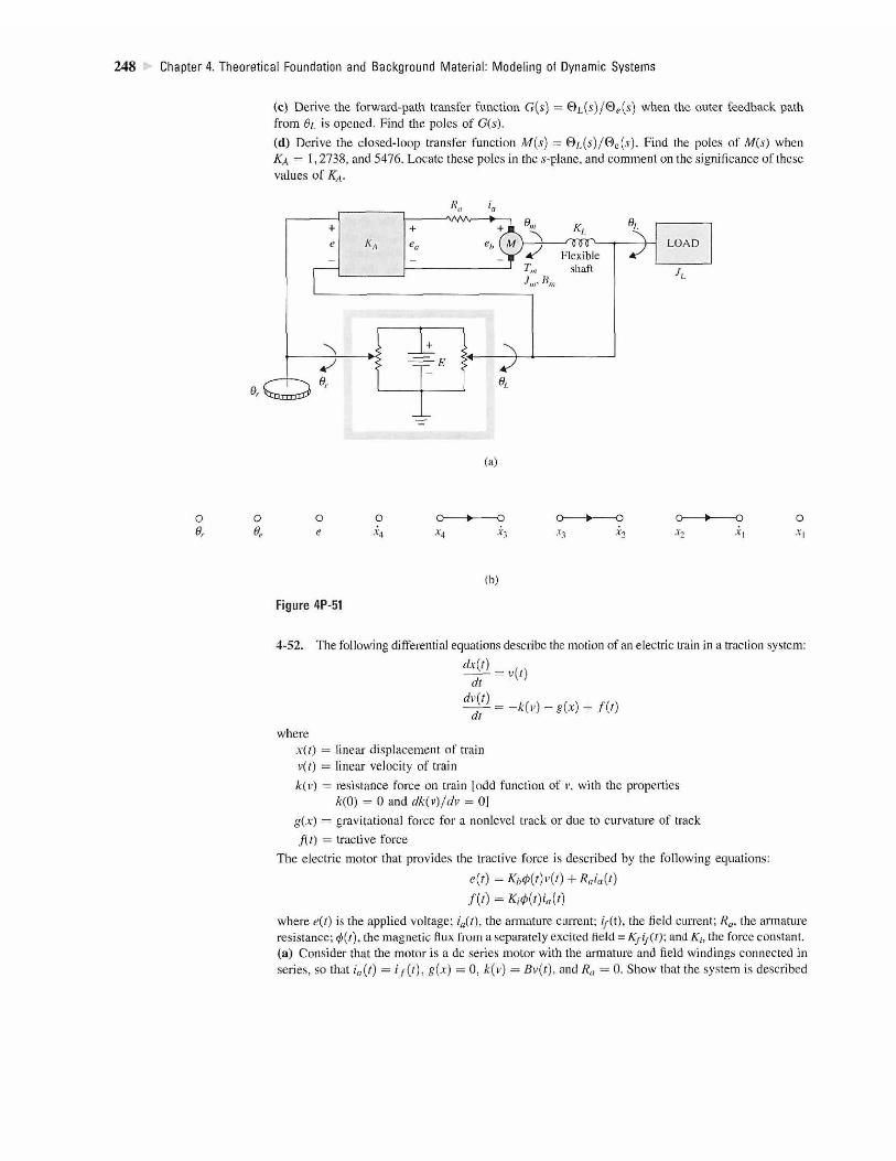
4-51. A dc-motor position-control system is shown in Fig. 4P-51(a). The following parameters and variables are defined: e is the error voltage; er, the reference input; 0/., the load position; KA, the amplifier gain; ea, the motor input voltage; eb, the back emf; /„, the motor current; T„„ the motor torque; 7,,,, the motor inertia = 0.03 oz-in.-s2; 5,,,, the motor viscous-friction coefficient = 10 oz-in.-s2; KL, the torsional spring constant = 50,000 oz-in./rad; //,, the load inertia = 0.05 oz-in.-s2; Kh the motor torque constant = 21 oz-in./A; K/,, the back-emf constant = 15.5 V/1000 rpm; Ks, the error-detector gain = £/27t; E, the error-detector applied voltage = In V; R0, the motor resistance = 1.15 ft; and Be = Qr - 0L-

(a) Write the state equations of the system using the following state variables: x\ — 0/., xi = dOt/dt = coi, .¥3 = 03, and XA = d6m/dt = com.

(b) Draw a signal flow diagram using the nodes shown in Fig. 4P-51(b).

248 Chapter 4. Theoretical Foundation and Background Material: Modeling of Dynamic Systems

(c) Derive the forward-path transfer function G(s) = ¢)^(5)/0,,(.9) when the outer feedback path from 6L is opened. Find the poles of G(s).

(d) Derive the closed-loop transfer function M(s) = ®z,(^)/©e(-^)- Find the poles of M(s) when KA = 1,2738, and 5476. Locate these poles in the .s-plane, and comment on the significance of these values of KA.

WnJ

U)

0

•*4 .v4 •v3

O

(b)

Figure 4P-51

4-52. The following differentia] equations describe the motion of an electric train in a traction system:

dx{t)

dt dv{t)

dt

= v(t)

= ~k(v)~g{x) /(0 where

x(t) = linear displacement of train v(/) = linear velocity of train

k(v) = resistance force on train [odd function of v, with the properties k(0) = 0 and dk{v)/dv = Oj

g(x) = gravitational force for a nonlevel track or due to curvature of track

/(/) = tractive force

The electric motor that provides the tractive force is described by the following equations:

e{t) = Kh<t>{t)v{t) + RJa{t)

f{t) = Ki<f>(t)ia(t)

where e(t) is the applied voltage; ia(t), the armature current; i/(t), the field current; Ra, the armature resistance; ¢(/), the magnetic flux, from a separately excited field = Kjif(t); and Kt, the force constant, (a) Consider that the motor is a dc series motor with the armature and field windings connected in series, so that ia(t) = i/(t), g(x) = 0, k(v) = Bv(t), and R(, — 0. Show that the system is described

Problems 249

by the following nonlinear state equations:

dx{t

dt dv(t)

dt

= v(t)

= -Bvfj) K,

KlKfvHt) e\t)

(b) Consider that, for the conditions stated in part (a), ia(t) is the input of the system [instead of £•(/)]. Derive the state equations of the system.

(c) Consider the same conditions as in part (a) but with 0(f) as the input. Derive the state equations.

4-53. The linearized model of a robot arm system driven by a dc motor is shown in Fig. 4P-53. The system parameters and variables are given as follows:

DC Motor Robot Arm

Tm = motor torque = K,ia K, = torque constant /„ = armature current of motor

J,,,= motor inertia Bm = motor viscous-friction coefficient

B = viscous-friction coefficient of shaft between the motor and arm

BL = viscous-friction coefficient of the robot arm shaft

JL = inertia of arm TL — disturbance torque on arm 6l = arm displacement K = torsional spring constant

6,,, — motor-shaft displacement

(a) Write the differential equations of the system with ia{t) and TL(l) as input and 9m(t) and $/_(t) as outputs.

(b) Draw an SFG using Ia(s), TL(s), ®„,{s). and6/.(5) as node variables.

(c) Express the transfer-function relations as

Find G(,v).

= G(,) Ia(s)

-TL(S)

Robot

Figure 4P-53

250 Chapter 4. Theoretical Foundation and Background Material: Modeling of Dynamic Systems

PROBLEMS FOR SECTION 4-8 4-54. The transfer function of the heat exchanger system is given by

T{s) Ke~T«s

G{s) = r A(.v) (r,.v+l)(r2.?

where Tj is the time delay. (a) Plot the roots and zeros of the system.

(b) Use MATLAB to verify your answer in part (a).

4-55. Find the polar plot of the following functions by using the approximation of delay function described in Section 2.8.

(a) G(s) =

(b) G{s) =

(Ts+l)

2 + 2se" + 4e -7s

s2 + 3s + 2 4-56. Use MATLAB to solve Problem 4-55 and plot the step response of the systems.

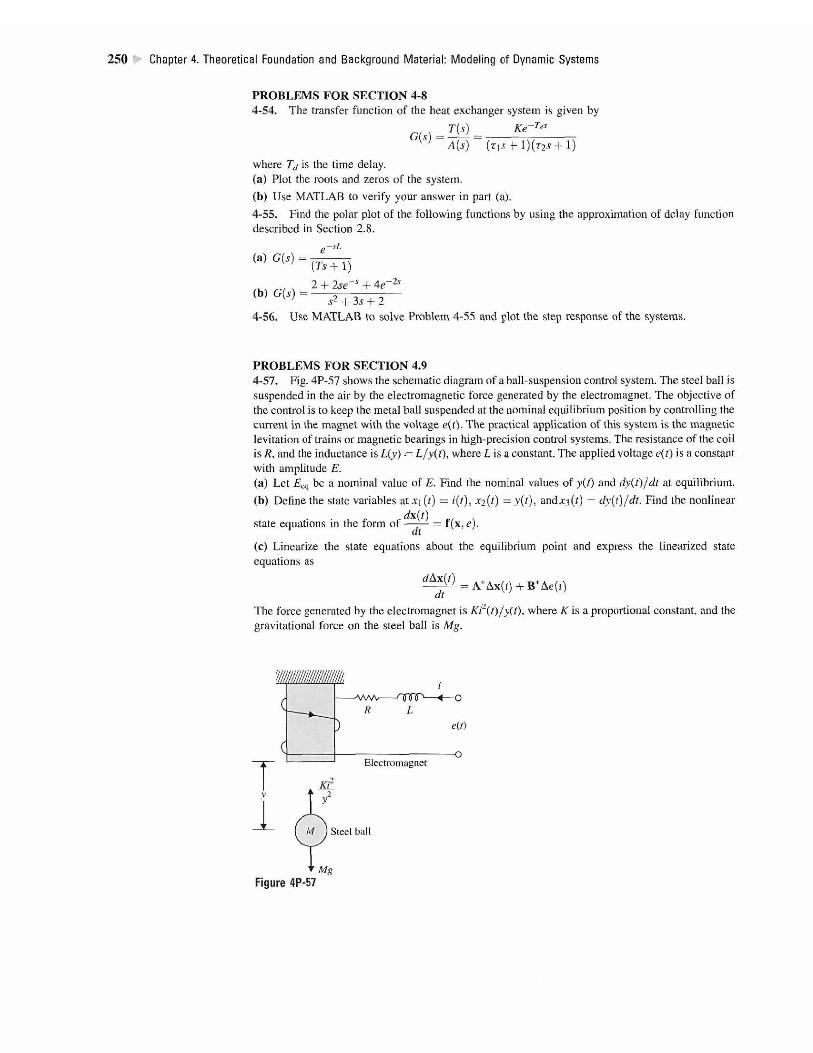
PROBLEMS FOR SECTION 4.9 4-57. Fig. 4P-57 shows the schematic diagram of a ball-suspension control system. The steel ball is suspended in the air by the electromagnetic force generated by the electromagnet. The objective of the control is to keep the metal ball suspended at the nominal equilibrium position by controlling the current in the magnet with the voltage e(t). The practical application of this system is the magnetic levitation of trains or magnetic bearings in high-precision control systems. The resistance of the coil is R, and the inductance is L(y) = L/y(t), where L is a constant. The applied voltage e(t) is a constant with amplitude E. (a) Let Eea be a nominal value of E. Find the nominal values of y(t) and dy{t)/dt at equilibrium.

(b) Define the state variables vAx\{t) = i(t), X2(t) = y{t), and *3 (/) = dy{t)/dt. Find the nonlinear dx(t) .

state equations in the form of —-— = f(x, e).

(c) Linearize the state equations about the equilibrium point and express the linearized state equations as

dAx{t) dt

= A*Ax(r) + B*Ae(/)

The force generated by the electromagnet is Ki2(t)/y(t), where AT is a proportional constant, and the gravitational force on the steel ball is Mg.

R I e(i)

Electromagnet

M Steel ball

Figure 4P-57

Problems 251

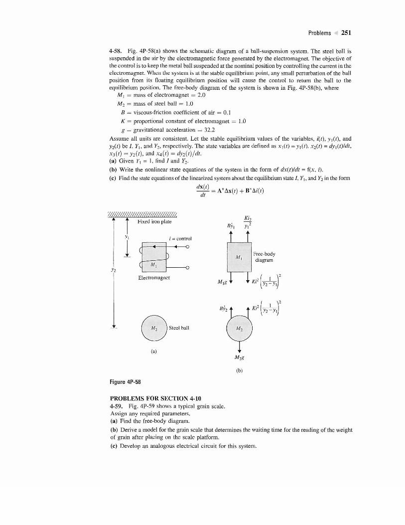
4-58. Fig. 4P-58(a) shows the schematic diagram of a ball-suspension system. The steel ball is suspended in the air by the electromagnetic force generated by the electromagnet. The objective of the control is to keep the metal ball suspended at the nominal position by controlling the current in the electromagnet. When the system is at the stable equilibrium point, any small perturbation of the ball position from its floating equilibrium position will cause the control to return the ball to the equilibrium position. The free-body diagram of the system is shown in Fig. 4P-58(b), where

M| = mass of electromagnet = 2.0 M2 = mass of steel ball = 1.0

B = viscous-friction coefficient of air = 0.1

K = proportional constant of electromagnet = 1 . 0

g — gravitational acceleration = 32.2 Assume all units are consistent. Let the stable equilibrium values of the variables, i(t), y\(t), and y2(t) be I, Y], and Y2, respectively. The state variables are defined as X\{t) = yt(f), x2(t) = dy\{t)ldt, **C0 =>'2(/), and x4(t) = dy2(t)/dt.

(a) Given r , = 1, find / and Y2.

(b) Write the nonlinear state equations of the system in the form of dx{t)ldt = f(.v, i).

(c) Find the state equations of the linearized system about the equilibrium state I, Y\, and Y2 in the form

dx(t) dt

= A*Ax(r) + B*A/(r)

7/////////////////////////////////, Fixed iron plate

y\

yi

Electromagnet

(a)

; 2 | _ L y'2-y\

Figure 4P-58

PROBLEMS FOR SECTION 4-10 4-59. Fig. 4P-59 shows a typical grain scale. Assign any required parameters. (a) Find the free-body diagram.

(b) Derive a model for the grain scale that determines the waiting time for the reading of the weight of grain after placing on the scale platform.

(c) Develop an analogous electrical circuit for this system.

252 Chapter 4. Theoretical Foundation and Background Material: Modeling of Dynamic Systems

Figure 4P-59

4-60. Develop an analogous electrical circuit for the mechanical system shown in Figure 4P-60.

Figure 4P-60

4-61. Develop an analogous electrical circuit for the fluid hydraulic system shown in Fig. 4P-61.

I h

1 Q Q

Figure 4P-61

PROBLEMS FOR SECTION 4-11 4-62. The open-loop excitation model of the car suspension system with 1-DOF, illustrated in Fig. 4-84(c), is given in Example 4-11-3. Use MATLAB to find the impulse response of the system.

4-63. An active control designed for the car suspension system with 1 -DOF is designed by using a dc motor and rack. Use MATLAB and the transfer function of the system given in Example 4-11-3 to plot the impulse response of the system. Compare your result with the result of Problem 4-62.

5 Time-Domain Analysis of Control Systems

In this chapter, we depend on the background material discussed in Chapters 1-4 to arrive at the time response of simple control systems. In order to find the time response of a control system, we first need to model the overall system dynamics and find its equation of motion. The system could be composed of mechanical, electrical, or other sub-systems. Each sub-system may have sensors and actuators to sense the environment and to interact with it. Next, using Laplace transforms, we can find the transfer function of all the sub-components and use the block diagram approach or signal flow diagrams to find the interactions among the system components. Depending on our objectives, we can manipulate the system final response by adding feedback or poles and zeros to the system block diagram. Finally, we can find the overall transfer function of the system and, using inverse Laplace transforms, obtain the time response of the system to a test input—normally a step input.

Also in this chapter, we look at more details of the time response analysis, discuss transient and steady state time response of a simple control system, and develop simple design criteria for manipulating the time response. In the end, we look at the effects of adding a simple gain or poles and zeros to the system transfer function and relate them to the concept of control. We finally look at simple proportional, derivative, and integral controller design concepts in time domain. Throughout the chapter, we utilize MATLAB in simple toolboxes to help with our development.

5-1 TIME RESPONSE OF CONTINUOUS-DATA SYSTEMS: INTRODUCTION

Because time is used as an independent variable in most control systems, it is usually of interest to evaluate the state and output responses with respect to time or, simply, the time response. In the analysis problem, a reference input signal is applied to a system, and the performance of the system is evaluated by studying the system response in the time domain. For instance, if the objective of the control system is to have the output variable track the input signal, starting at some initial time and initial condition, it is necessary to compare the input and output responses as functions of time. Therefore, in most control-system problems, the final evaluation of the performance of the system is based on the time responses.

The time response of a control system is usually divided into two parts: the transient response and the steady-state response. Let y(t) denote the time response of a continuous-data system; then, in general, it can be written as

y(t)=yt(t)+y5S(t) (5-D

253