Embed Size (px)
Citation preview

History Concept Importance Manual Formula Software Package Experience Curve Societal Impact
The Learning CurveThe Learning Curve Phenomenon Phenomenon
Applied Management Science for Decision Making, 1e Applied Management Science for Decision Making, 1e © 2012 Pearson Prentice-Hall, Inc. Philip A. Vaccaro , PhD© 2012 Pearson Prentice-Hall, Inc. Philip A. Vaccaro , PhD

The Learning CurveThe Learning CurveHISTORY
Introduced by Theodore Paul Wright in Factors Affecting The Cost of Airplanes, Journal of Aero Science ( 1936 )
The article covered the role of learning in the airplane production process, the methods of measuring learning, and the effect of learning on plane production volume and costs

Theodore Paul WrightTheodore Paul Wright1895 - 19701895 - 1970
M.I.T. ( 1918 ) - graduate, aeronautical engineering
Naval Reserve Officer ( WW I )
Curtiss Aeroplane Company - executive engineer (1921) - chief engineer (1925) - plant manager (1931) - vice-president, engineering (1935)
Office of Production Management - assistant director, aircraft (1942-1945)
Cornell University - acting president (1951) - vice-president, research (1948-1960)

The Learning Curve ConceptThe Learning Curve Concept
THIS APPLIES TO INDIVIDUALS,DEPARTMENTS, FIRMS, AND
ENTIRE INDUSTRIES
If a task is performedrepeatedly over time,its performance timewill drop dramaticallyand then continue todrop at a slower rateuntil a leveling off is
reached

80% Learning Curve80% Learning CurveINTERPRETATIONINTERPRETATION
If the base unit (1st unit) needed 200 hours of labor, then the doubled base unit (2nd unit) will only need 160 hours of labor.
If the base unit (2nd unit) needed 160 hours of labor, then the doubled base unit (4th unit) will only need 128 hours of labor.
[ 200 x .80 = 160 ]
[ 160 x .80 = 128 ]

80% Learning Curve80% Learning CurveINTERPRETATIONINTERPRETATION
If the base unit (4th unit) needed 128 hours of labor, then the doubled base unit (8th unit) will only need 102.4 hours of labor.
If the base unit (8th unit) needed 102.4 hours of labor, then the doubled base unit (16th unit) will only need 81.92 hours of labor.
128 x .80 = 102.4
102.4 x .80 = 81.92

80% Learning Curve80% Learning Curve
0 1 2 4 8 16 32
200 hours
150 hours
100 hours
50 hours
0 hours
UNITS
GRAPHGRAPH
LABOR HOURS
NegativeExponential
Curve
1st unit requires 200 hours 2nd unit requires 160 hours 4th unit requires 128 hours 8th unit requires 102 hours16th unit requires 82 hours

The Learning CurveThe Learning Curve
UNIT 70% 80% 90%
1st 200 200 200
2nd 140 160 180
4th 98 128 162
8th 68.6 102 145.8
16th 48.02 82 131.2
32nd 33.61 65.6 118.1
THE LOWER THE PERCENTAGE, THE MORE EFFICIENTTHE LOWER THE PERCENTAGE, THE MORE EFFICIENT
THE NORMAL RANGETHE NORMAL RANGE
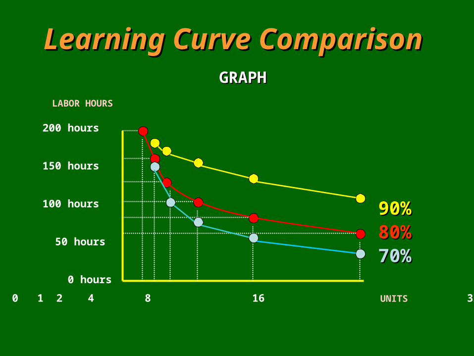
Learning Curve ComparisonLearning Curve Comparison
0 1 2 4 8 16 32
200 hours
150 hours
100 hours
50 hours
0 hours
UNITS
GRAPHGRAPH
LABOR HOURS
80%80%70%70%
90%90%

The Learning CurveThe Learning CurveOTHER FACTORS REFLECTEDOTHER FACTORS REFLECTED
Improvements in layout design. Changes in product materials. Changes in work methods. Changes in labor policies. Engineering modifications. Equipment replacement. Equipment redesign. Worker training.

The Learning Curve PhenomenonThe Learning Curve PhenomenonOTHER APPLICATIONS
LABOR COST ESTABLISHMENT
SUBCONTRACTING DECISIONS
STRATEGIC EVALUATION OF THE FIRM IN ITS INDUSTRY
PURCHASING DECISIONS
LABOR SCHEDULING
LABOR BUDGETING
Learning Curve ImportanceLearning Curve Importance
Premature depletions of materials and components on the production line are avoided entirely.
Customer orders need not be rejected based on the mistaken notion that the factory is “booked solid” in the immediate future.
Human resources need not hire additional workers to meet future product demand.
It may eliminate or defer the need for factory expansion or new construction.

The Learning Curve FormulaThe Learning Curve Formula
• A firm historically has had an 85% learning curve.
• The 1st unit of a new product is estimated to require 3,000 labor hours.
• The firm wants to know how many labor hours will be needed for the 50th unit.
APPLICATIONAPPLICATION

The LearningThe Learning Curve FormulaCurve Formula
Y = Y x Nn 1
x
where:
Y = time required for a specific unit
Y = time required for the 1st unit
N = the unit for which a time is sought
the learning rate
n
1
x / r =

The Learning Curve FormulaThe Learning Curve FormulaEXECUTIONStep 1
Compute the learning rate: the sensitivity of unit labor time to cumulative productive output
X = natural logarithm of the learning curve
natural logarithm of 2.0
X =natural logarithm of “ .85 “
natural logarithm of “ 2.0 “
X =- .162518
.693147= - .23446
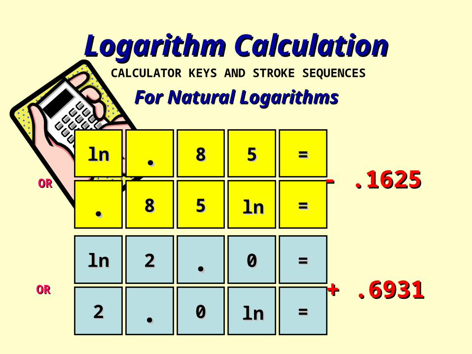
Logarithm CalculationLogarithm Calculation CALCULATOR KEYS AND STROKE SEQUENCES
For Natural LogarithmsFor Natural Logarithms
lnln
..
lnln
22
88
22
..
88
55
..
00
55
00
==
==
==
==
..OROR - .1625- .1625
OROR + .6931+ .6931
lnln
lnln

Logarithm CalculationLogarithm Calculation CALCULATOR KEYS AND STROKE SEQUENCES
For ‘Base 10’ LogarithmsFor ‘Base 10’ Logarithms
log
.
log
2
8
2
.
8
5
.
0
5
0
=
=
=
=
.OROR - .070581- .070581
OROR + .30103+ .30103
log 10x
log 10x

The Learning Curve FormulaThe Learning Curve FormulaEXECUTION
Step 2Insert the values of all variables in the general formula:
Y = Y Nn 1.
x
becomes:
Y = 3,000 x 50- .23446
50
= 3,000 x 1
2.5023065
= 3,000 x .39963
= 1,198.9hours required toproduce the 50th
unit in the series
50- .23446
becomes…..
1
50+ .23446
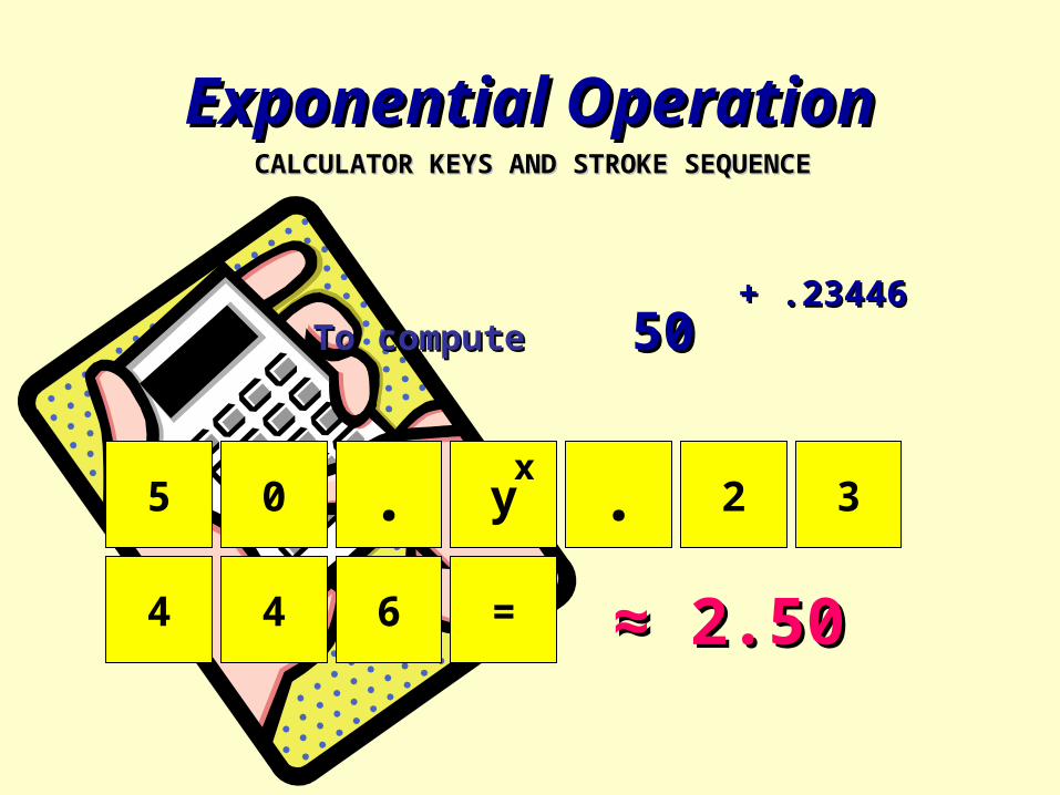
Exponential OperationExponential OperationCALCULATOR KEYS AND STROKE SEQUENCECALCULATOR KEYS AND STROKE SEQUENCE
To computeTo compute 50 50 + .23446+ .23446
5 0 . y . 2 3
4 4 6 =
x
≈ ≈ 2.50 2.50

Exponential OperationExponential OperationCALCULATOR KEYS AND STROKE SEQUENCECALCULATOR KEYS AND STROKE SEQUENCE
To computeTo compute 50 50 + .23446+ .23446
5 0 . . 2 3
4 4 6 = ≈ ≈ 2.50 2.50
Λ
FOUND ON NEW CALCULATORS

Learning Curve with QM for WINDOWSLearning Curve with QM for WINDOWS
MANAGEMENTMANAGEMENTFOR THEFOR THE
2121stst
CENTURYCENTURY

We Select This Module
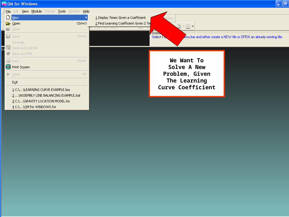
We Want ToSolve A New
Problem, GivenThe Learning
Curve Coefficient

TheDialogue Box
Appears

The Data TableLooks Like This,
With The Base UnitAutomatically
The 1st Unit

THE NUMBER OFHOURS TO MAKE
THE 1st UNIT
THE UNIT FORWHICH WE WANT
TO FIND THENUMBER OF HOURS
THE LEARNINGCURVE OF 85%
( GIVEN )

THE 50th UNIT WILLTAKE 1,198.87
HOURS TO COMPLETE

THE 15th UNIT WILL TAKE1,589.896 HOURS TO
COMPLETE.CUMULATIVE PRODUCTION
HOURS AT THAT POINTARE 29,583.17 HOURS

THE 50th UNIT, OFCOURSE, WILL TAKE
1,198.87 HOURSTO COMPLETE
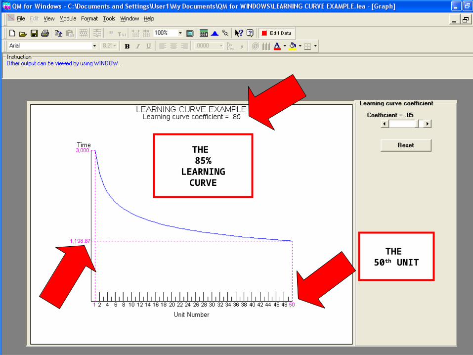
THE 85%
LEARNINGCURVE
THE 50th UNIT

WE CAN CHANGETHE LEARNING CURVE
TO 75% BYADJUSTING THE
COUNTERTHE 50th UNIT
WOULD THEN TAKEONLY 591.54HOURS TO
COMPLETE !

THE 95%LEARNING CURVE
CAN ALSO BEFOUND
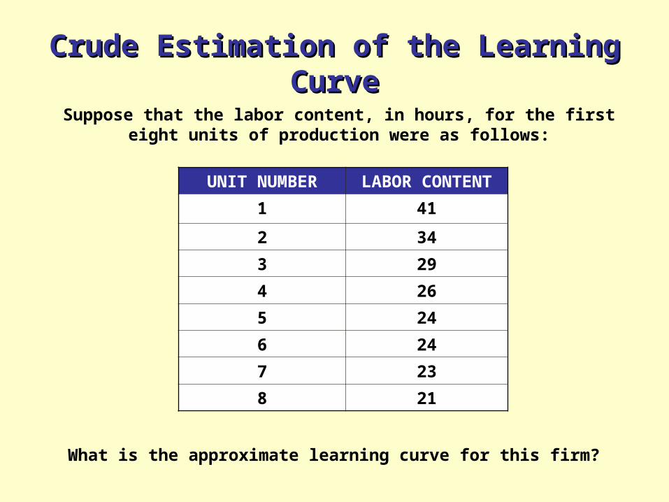
Crude Estimation of the Learning CurveCrude Estimation of the Learning Curve
Suppose that the labor content, in hours, for the firsteight units of production were as follows:
UNIT NUMBER LABOR CONTENT
1 41
2 34
3 29
4 26
5 24
6 24
7 23
8 21
What is the approximate learning curve for this firm?

We Select ThisSub Menu
To Estimate TheLearning Curve

THE DIALOGUEBOX

THE DATA INPUT TABLEREQUIRES THE NUMBER OFHOURS IT TOOK TO MAKE
THE 1st UNIT AND THENUMBER OF HOURS IT
TOOK TO MAKE A LATER UNIT( YOUR CHOICE )

WE CHOSE TO USE THE8th UNIT IN THE SERIES
WITH 21 HOURS OFACTUAL PRODUCTION
TIME

THE ESTIMATEDLEARNING CURVE,
BASED ON THE 1st AND 8th UNITSPRODUCED, IS
80%

THE ESTIMATED
80%LEARNING
CURVE

THE PROGRAM’SESTIMATED
PRODUCTIONHOURS
FOR UNITS 1 THROUGH 8
ACTUAL HOURS
1st UNIT - 412nd UNIT - 343rd UNIT - 294th UNIT - 265th UNIT - 246th UNIT - 247th UNIT - 238th UNIT - 21

The Learning Curve The Learning Curve PhenomenonPhenomenon
Applied Management Science for Decision Making, 1e Applied Management Science for Decision Making, 1e © 2012 Pearson Prentice-Hall, Inc. Philip A. Vaccaro, PhD© 2012 Pearson Prentice-Hall, Inc. Philip A. Vaccaro, PhD


Just-in-Time SystemsJust-in-Time SystemsJIT
• History• Concept• System Elements• System Operation• Prerequisites• Selected Applications MANUFACTURING AND SERVICE
Applied Management Science for Decision Making, 1e Applied Management Science for Decision Making, 1e © 2012 Pearson Prentice-Hall, Inc. Philip A. Vaccaro , PhD© 2012 Pearson Prentice-Hall, Inc. Philip A. Vaccaro , PhD

Just-in-Time SystemsJust-in-Time SystemsHISTORYHISTORY
THE LITTLE KNOWN ORIGIN OF JIT
In 1912 Ford Motor Company begins using ferries to ship automobile hoods, doors, and
trunk lids from its factories on the east side of Lake Erie to its assembly plants in Detroit on
a twice-daily basis, and in the quantities needed to support daily production
Just-in-Time SystemsJust-in-Time SystemsHISTORYHISTORY
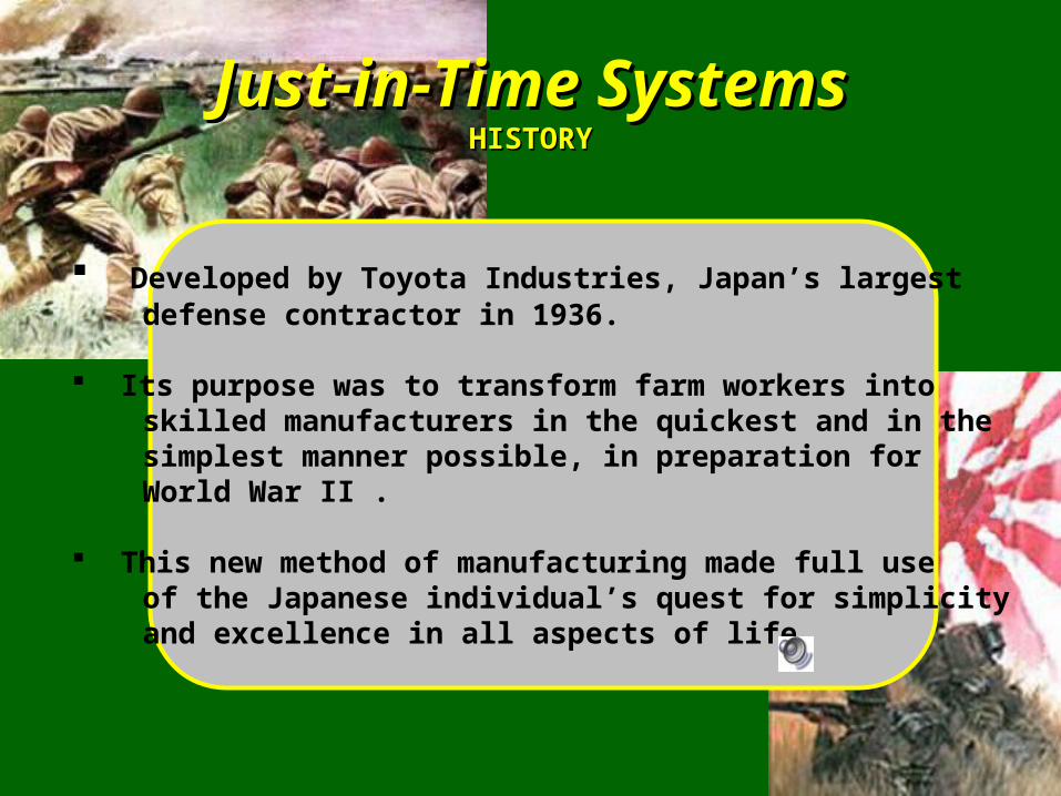
Developed by Toyota Industries, Japan’s largest defense contractor in 1936.
Its purpose was to transform farm workers into skilled manufacturers in the quickest and in the simplest manner possible, in preparation for World War II .
This new method of manufacturing made full use of the Japanese individual’s quest for simplicity and excellence in all aspects of life.

Just-in-Time SystemsJust-in-Time SystemsTHE CONCEPTTHE CONCEPT
A part, subassembly, or material is pulled through the system to wherever it is needed, exactly when it is needed. This “pull” system is employed both by the factory and its external suppliers.
This “pull” system utilizes signaling devices to request production and delivery from upstream centers to downstream centers.
CENTERS ARE EITHER PRODUCTION OR MATERIAL SUPPLY

Just-in-Time SystemsJust-in-Time SystemsTHE CONCEPTTHE CONCEPT
The pulling of parts and materials through the system in small lots to wherever they are needed, when they are needed, removes the need for inventory cushions.
Elimination of inventory cushions exposes operational problems to the full light of day, which in turn, are then eliminated on a prioritized basis.
Continuous improvement is emphasized by the firm thereafter.
MANUFACTURING CYCLE TIMES ARE ALSO REDUCED

Excessive InventoriesExcessive InventoriesCONCEAL SERIOUS PROBLEMSCONCEAL SERIOUS PROBLEMS
Unreliable deliveries of materials & components. Lost production due to defective materials.
Improper human and equipment processing. Delays caused by long setup times and machine breakdowns.
Managerial incompetency in planning, ordering, and scheduling.
FIRMS USE INVENTORIES TO MASK THEIR MISTAKES

Draining The Inventory LakeDraining The Inventory Lake
POORSCHEDULING
IMPROPEREQUIPMENTOPERATION
EQUIPMENTBREAKDOWNS
LATEDELIVERIES
DEFECTIVEMATERIALS
AS INVENTORY LEVELSARE SYSTEMATICALLY
REDUCED, OPERATIONALPROBLEMS MAKE THEIR
APPEARANCE
ROCKSROCKS

The Two-Card Scheduling System THE PRODUCTION CARD
Issued by a downstream work center to one or more upstream manufacturing
work centers
Authorizes delivery of a previouslyproduced tray of parts/subassemblies,
or new production of a tray of same,in order to replenish a tray sent earlier
PRODUCTIONCARD
LOOKS LIKE ANOLD COMPUTERPUNCH CARD

BASICALLY,
A MATERIALS
REQUISITION
ORDER
The Two-Card Scheduling SystemTHE MOVE CARDTHE MOVE CARD
Issued by a downstream work centerto one or more upstream supply centers
located across the street or up to 100 miles away !
Authorizes delivery of a previouslyproduced tray of materials/supplies, or
another delivery of same, in order toreplenish a tray sent earlier

The Two-Card Scheduling SystemKANBAN CONCEPT & PRACTICE
USERUSERCENTERCENTER
SUPPLYSUPPLYCENTERCENTER
MFG.CENTER
MOVECARD
PRODUCTIONCARD
TRAYTRAYOFOF
MATERIALSMATERIALS
TRAYTRAYOFOF
PARTSPARTS
THEDOWNSTREAM
CENTER
THE UPSTREAM
CENTER
THE UPSTREAM
CENTER
sends
sends
receives
receives
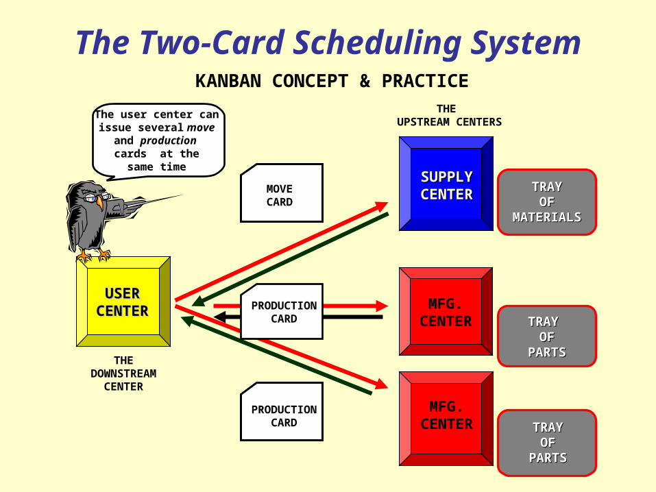
The Two-Card Scheduling SystemKANBAN CONCEPT & PRACTICE
USERUSERCENTERCENTER
SUPPLYSUPPLYCENTERCENTER
MFG.CENTER
MOVECARD
PRODUCTIONCARD
TRAYTRAYOFOF
MATERIALSMATERIALS
TRAYTRAYOFOF
PARTSPARTS
THEDOWNSTREAM
CENTER
THE UPSTREAM CENTERS
MFG.CENTER TRAY TRAY
OFOFPARTSPARTS
PRODUCTIONCARD
The user center canissue several move
and production cards at thesame time

STREETSTREET
The Two-Card Scheduling SystemCYCLISTS CARRIED EMPTY TRAYS AND FILLED TRAYS BETWEEN FACTORY AND VENDORS
STREETSTREET
MAINASSEMBLY
PLANT GLASSPRODUCER
METALPART
PRODUCER
SSTTRREEEETT
SSTTRREEEETT
EMPTYEMPTY
TRAY TRAY
EMPTY
EMPTY
TRAYTRAY
CARDCARD
CCEENNTTEERR
CCEENNTTEERR
INDUSTRIAL PARKINDUSTRIAL PARK
FILLEDFILLED
TRAYTRAY CARD
FILLEDFILLED
TRAYTRAY

The Two-Card Scheduling System
100 mile100 mile
radiusradius
GLASSMFG
CHIPMFG
METALMFG
ASSEMBLYPLANT
HARDWAREMFGCOATINGS
MFG
WHEN THEDISTANCES
ARESUBSTANTIAL
STANDINGSTANDINGPURCHASEPURCHASE
AGREEMENTSAGREEMENTSREPLACE
MOVECARDS
TRUCKS, PLANES,
AND TRAINSREPLACEREPLACEBICYCLES

The Two-Card Scheduling System
Standing purchase agreements with external vendors for a specific number of trays of parts or materials to be delivered daily by truck, rail, boat, or plane, at dawn or mid-day, or both.
Flashing lights, bells, whistles, rags, and flags between the work centers.
E-commerce isincreasingly
popular
PRODUCTION AND MOVE CARD ALTERNATIVESPRODUCTION AND MOVE CARD ALTERNATIVES
OVER LONG DISTANCES
WITHIN THE PLANT ITSELF

The Two-Card Scheduling SystemKANBAN CONCEPT & PRACTICE
USERUSERCENTERCENTER
SUPPLY SUPPLY oror
MFGMFGCENTERCENTER
USERUSERCENTERCENTER
SUPPLYSUPPLYoror
MFGMFGCENTERCENTER
EMPTYEMPTYTRAYTRAY
EMPTYEMPTYTRAYTRAY
( NO CARD )( NO CARD )
TO REFILL
CARD
TO STOP REFILL
SENDS

The Two-Card Scheduling SystemKANBAN CONCEPT & PRACTICE
EMPTY TRAYEMPTY TRAY( NO CARD )( NO CARD )
SUPPLYSUPPLYoror
MFGMFGCenterCenter
REFILLEDREFILLEDTRAYTRAY
WHEN AN EMPTY TRAY IS RETURNED
WITH NO CARD, IT IS IMMEDIATELY
REFILLED AND KEPT UNTIL IT IS ONCE
AGAIN NEEDED BY THE USER CENTER.
THIS COULD BE THE NEXT
DAY OR THE SAME
AFTERNOON

The Kanban TrayThe Kanban Tray
holds a particular part or subassembly.
holds a prescribed number of parts or subassemblies.
lined with foam or silk in order to avoid damaging the contents when moved from center to center.
compartments are shaped so as to accom- modate only properly-crafted parts or sub- assemblies.
usually carried by hand from center to center.

The Kanban TrayThe Kanban Tray
ONE ONE TYPETYPEPARTPART
ORORMATERIALMATERIAL
UNITUNIT
FOAM-LINEDFOAM-LINED COMPARTMENTSCOMPARTMENTS
CUTOUTS ONLY CUTOUTS ONLY ACCOMMODATE ACCOMMODATE
PROPERLY MADE PROPERLY MADE UNITSUNITS

The Kanban Tray / BinThe Kanban Tray / BinCALCULATING THE NUMBER REQUIREDCALCULATING THE NUMBER REQUIRED
MANAGEMENT MUST FIRST ESTABLISH THE NUMBER OF
COMPARTMENTS WITHIN EACH TRAY / BIN AND ITS SIZE
The number of trays / bins sets the amount of
authorized inventory for a particular part
or material
It is based on the item’s daily demand, production lead time, and safety stock
needed to compensatefor system uncertainty

““Authorized Inventory”Authorized Inventory”
JIT system manufacturing is also known as “stockless production”, that is, daily manufacturing without stand- ing beginning or work-in-process inventories.
In reality however, there will always be some permanent inventories in the JIT system, usually 1% to 2% of the ori- ginal amounts.
These inventories are the pre-made parts, subassemblies, and materials that are contained in the kanban trays.
Their purpose is to quickly start production on that same afternoon or next day, rather than wait for items to be pro- duced from scratch.

The Kanban TrayThe Kanban TrayTHE NUMBER FORMULATHE NUMBER FORMULA
Numberof
Trays=
Lead Time Demand + Safety Stock
Number of Tray Compartments
DAILY DEMAND - CAMERA “X” = 12 UNITS ( world-wide ) THEREFORE……. DAILY DEMAND - CAMERA “X” LENS ASSEMBLY = 12 UNITS ( derived ) DAILY DEMAND - CAMERA “X” HOUSING = 12 UNITS ( derived ) PRODUCTION LEAD TIME = 30 MINUTES ( 1/2 HOUR ) FOR EACH WORK CENTER SAFETY STOCK = 3 UNITS FOR EACH WORK CENTER
FROM THECAMERAEXAMPLE( TEXT )

The Kanban SystemThe Kanban System
FINALFINALASSEMBLYASSEMBLY
AREAAREA
CAMERACAMERAHOUSINGHOUSING
WORKWORKCENTERCENTER
CAMERACAMERALENSLENS
WORK WORK CENTERCENTER
PRODUCTIONCARD
PRODUCTIONCARD
TRAYTRAYCAMERACAMERA
““X”X”HOUSINGSHOUSINGS
TRAYTRAYCAMERACAMERA
““X”X”LENSESLENSES
WHERE THEHOUSING
ANDLENS
ASSEMBLIESCOME
TOGETHER
SENT
SENT
TRAYSDELIVERED
HOW MANY TRAYSAUTHORIZED ?
Calculating the Number of Trays

Lead Time Demand
Lead Time is the time required to prepare for a component or assembly
production run.
The firm needs to produce additionalunits in order to compensate
for this loss of time

The Kanban TrayThe Kanban TrayTHE NUMBER FORMULA
=Lead Time Demand + Safety Stock
Number of Tray Compartments
=[ 12 units x 1/16th day ] + 3 units
6 compartments
=[ 12 x .0625 ] + 3
6
DAILY DEMAND LEAD TIME
ONE TRAYEACH FORHOUSINGSAND LENS
ASSEMBLIES( CAMERA “X” )
= .625 ≈ 1 tray
Ifdaily
demandequals
12units

The Kanban TrayThe Kanban TrayTHE NUMBER FORMULA
=Lead Time Demand + Safety Stock
Number of Tray Compartments
=[ 120 units x 1/16th day ] + 3 units
6 compartments
=[ 120 x .0625 ] + 3
6
DAILY DEMAND LEAD TIME
TWO TRAYSEACH FORHOUSINGSAND LENS
ASSEMBLIES( CAMERA “X” )
= 1.75 ≈ 2 trays
Ifdaily
demandequals
120units

The Kanban TrayThe Kanban TrayTHE NUMBER FORMULA
=Lead Time Demand + Safety Stock
Number of Tray Compartments
=[ 500 units x 1/16th day ] + 3 units
6 compartments
=[ 500 x .0625 ] + 3
6
DAILY DEMAND LEAD TIME
SIX TRAYSEACH FORHOUSINGSAND LENS
ASSEMBLIES( CAMERA “X” )
= 5.71 ≈ 6 trays
THERE COULDBE THREE
OTHERCAMERAMODELS
THAT USECAMERA ‘X’s
HOUSINGSANDLENS
ASSEMBLIESWITH A
COMBINEDDEMANDOF 500

The Kanban BinThe Kanban BinTHE NUMBER FORMULATHE NUMBER FORMULA
=Lead Time Demand + Safety Stock
Size of Container
=[ 500 bolts x 2 days ] + 250 bolts
250 bolts ( bin size )
=[ 1,000 ] + 250
250
DAILY DEMAND LEAD TIME
5bins
neededfor this
item
2nd
EXAMPLEpartor
assembly
= 5 bins

Small Batch SizesSmall Batch Sizes
JIT systems use the smallest batch sizes possible.
They reduce the average level of inventory.
They pass through the system faster.
They allow for relatively early detection of any quality problems.
They help achieve a uniform workload on the system.
They simplify scheduling.
They can be moved around more effectively, enabling schedulers to utilize capacities efficiently.
A batch is a quantity of products that are produced
together

Small Batch SizesSmall Batch Sizes
Unfortunately, small batch sizes increase the number of setups and total setup costs.
A setup is a set of activities needed to change or readjust a process between successive batches of different products.
Typically, a setup takes the same amount of time and money regardless of the batch size.
Traditionally, producers select the batch size that provides the most economical solution.
An equation similar to the EOQ inventory model is used to find the optimum batch size.

Optimal Batch Size FormulaOptimal Batch Size Formula
( 2 ) ( D ) ( s )
h√Where: D = daily demand for the product 2 = constant
s = setup time ( cost units or time units )
h = processing time ( cost units or time units )
A larger batch size is more economical than a smaller batch size if the setup times are long.

Batch Size Cost TradeoffBatch Size Cost Tradeoff
0 Optimal Batch Size ∞
Setuptime / cost
Processing time / cost
Co
st /
Tim
e
Total Cost
AS BATCH SIZE INCREASES, THE NUMBER OF SETUPS AND SETUP COSTS DECREASESAS BATCH SIZE INCREASES, THE NUMBER OF SETUPS AND SETUP COSTS DECREASES
UNFORTUNATELY LARGER BATCH SIZES INCREASE PRODUCTION TIME AND INVENTORY CARRY COSTSUNFORTUNATELY LARGER BATCH SIZES INCREASE PRODUCTION TIME AND INVENTORY CARRY COSTS

Batch Size FormulaBatch Size Formula
The camera plant uses the same assembly line to produce all its models.
The setup time for initiating production of camera ‘X’ is 30 minutes.
After setup, one camera can be assembled every 6 minutes.
The daily demand for camera ‘X’ is 12.EXAMPLE

Batch Size FormulaBatch Size Formula
( 2 ) ( D ) ( s )
h√√
( 2 ) ( 12 ) ( 30 )
6
Most Economical Batch Size ≈ 11 units
EXAMPLE
This means that we should produceapproximately eleven (11) units of
camera model ‘X’, everytime we pro-duce them. This will minimize the
total costs of processing and setup.

Batch Size FormulaBatch Size Formula
The bolt plant uses the same assembly line to produce all its output.
The setup time for initiating production of the concrete bolt is 2 days ( 960 minutes ) .
After setup, one bolt can be produced every 1 minute.
The daily demand for this bolt is 500 .EXAMPLE

Batch Size FormulaBatch Size Formula
( 2 ) ( D ) ( s )
h√√
( 2 ) ( 500 ) ( 960 )
1
Most Economical Batch Size ≈ 980 units
EXAMPLE

The Batch Size FormulaThe Batch Size Formula
The formula considered the impact of setup time on only oneone process or piece of equipment. ( It ignored the other centers.)
A larger batch will always result in higherhigher inventory storage and handling costs throughout the production process, lead- ing to several other types of waste and inefficiency.
Therefore, in JIT firms, the focus is shifted from identifying
the optimum batch size to reducing setup timesreducing setup times.
If setup times are decreased, then the most economical batch
size will automatically automatically be reduced.

The desired “ideal” batch size in JIT is considered to be “one” ( 1 unit ) .
Batch size could be reduced to one unit, if the setup time were able to be reduced to near zero over all batch sizes.
An effort would be made to reduce setup times to as close to zero as possible, at each work center in the JIT facility.
A near zero setup time would allow the firm to respond to real-time consumer product demand even faster !
The “Ideal” Batch Size The “Ideal” Batch Size

Assembly Line BalancingUNDER THE KANBAN SYSTEM
PROBLEMS ENCOUNTERED DURING PRODUCTION ARE PROBLEMS ENCOUNTERED DURING PRODUCTION ARE TEMPORARILY SOLVED BY SUPERVISORS, ENGINEERS, TEMPORARILY SOLVED BY SUPERVISORS, ENGINEERS, AND WORKERS IN ORDER TO KEEP THE LINE MOVING.AND WORKERS IN ORDER TO KEEP THE LINE MOVING.
The assembly line is rebalanced each timeanother product is started in production
Supervisors are positioned along the assembly line to ensure that each
work center is producing at the same pace as all the other work
centers

Assembly Line BalancingAssembly Line BalancingUNDER THE KANBAN SYSTEM
no maximum and minimum cycle times.
no minimum number of work stations.
no formal efficiency and effectiveness measures.
no standard task times.
BASICALLY THE WORK CENTERS ARE CONSIDERED TO BEPERFORMING ADEQUATELY AS LONG AS TRAYS ARE BEING
FILLED AND EMPTIED ON A TIMELY BASIS WITHIN THE PERIODSCHEDULED FOR A PARTICULAR PRODUCT’S PRODUCTION

The Kanban SystemThe Kanban SystemTEXT EXAMPLE – PARTIAL OVERVIEW
CORPORATEHQ
FINALFINALASSEMBLYASSEMBLY
AREAAREA
CAMERACAMERAHOUSINGHOUSING
WORKWORKCENTERCENTER
CAMERACAMERALENSLENS
WORK WORK CENTERCENTER
OVERNIGHTINCOMINGORDERS
PRODUCTIONCARD
PRODUCTIONCARD
TRAYTRAYCAMERACAMERA
““X”X”HOUSINGSHOUSINGS
TRAYTRAYCAMERACAMERA
““X”X”LENSESLENSES
PRODUCE12
MODEL “X”CAMERASAT 9:00 AM
SENT
SENT
TRAYSDELIVERED

The Kanban SystemThe Kanban SystemTEXT EXAMPLE – PARTIAL OVERVIEWTEXT EXAMPLE – PARTIAL OVERVIEW
COMPUTERCHIP
PRODUCERCAMERACAMERAHOUSINGHOUSING
WORKWORKCENTERCENTER
CAMERACAMERALENSLENS
WORK WORK CENTERCENTER
MOVE CARD
MOVE CARD
TRAYTRAYCAMERACAMERA
““X”X”CHIPSCHIPS
TRAYTRAYCAMERACAMERA
““X”X”RAWRAW
GLASSGLASS
Trays Delivered by Bike or Vehicle
RAWRAWGLASSGLASS
PRODUCERPRODUCER
Across the street or 100 MILES away
( TWO HOURS DRIVE TIME )
SENT
SENT

Successful JIT SystemsSuccessful JIT SystemsPREREQUISITES
Better equipment maintenance and repair Reliable materials deliveries Quick machine setups Worker empowerment Better process quality Better product quality

Dr. Shigeo ShingoDr. Shigeo ShingoTHE FATHER OF MACHINE SETUP REDUCTION
In 1950, this Mazda engineer discovered that setup operations consisted of two distinct activities: internal and external.
Internal activities are those performed when the equipment is stopped, i.e. changing an ink cartridge.
External activities are those performed while the equipment is still operating, i.e. unpacking an ink cartridge from its carton.
This discovery formed the basis of a procedure for reducing setup time called SMED ( single minute exchange of dies), named after a particular project but now applicable to any type of machine setup.
REDUCEDSETUP TIMES
ARE AMAJOR
JITCOMPONENT

The Goals of Setup Reduction
standardize sizes and shapes of molds standardize parts for easy insertion and removal use the same fasteners for each setup use pre-marked settings on dials and levers
I. Convert as many internal setup activities into external setup activities as possible, for quicker machine setups.
II. Reduce the external setup activities themselves.

Steps to Reduce Setup Times
Separate setup into preparation and actual setup,doing as much as possible while the
machine/process is operating( save 30 minutes )
Move material closer andimprove material handling
( save 20 minutes )
Standardize andimprove tooling
( save 15 minutes )
Use one-touch system toeliminate adjustments
( save 10 minutes )
Training operators andstandardizing work
procedures( save 2 minutes )
Repeat cycle untilsub-minute setup
is achieved
INITIAL SETUP TIME
Step 1
Step 2
Step 3
Step 4
Step 5
Step 6

Desired Setup Time FormulaDesired Setup Time FormulaOnce a lot size has been determined, the EOQ production orderquantity model can be modified to determine the desired setuptime. The original model is shown below:
Q* = 2DS
H [1 - ( d/p )]√ where:
D = annual demand S = setup cost H = carry cost d = daily demand p = daily production

Desired Setup Time ExampleDesired Setup Time Example
Flair Furniture, Inc., a firm that produces rustic furniture, desires to move toward a reduced lot size. Their production analyst, determined that a two hour production cycle would be acceptable be- tween two work centers. Further, the analyst concluded that a setup time that would accommodate the two hour cycle time should be achieved.
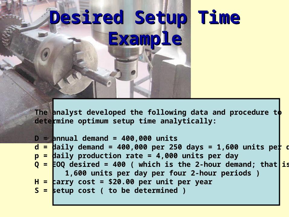
Desired Setup Time ExampleDesired Setup Time Example
The analyst developed the following data and procedure todetermine optimum setup time analytically:
D = annual demand = 400,000 unitsd = daily demand = 400,000 per 250 days = 1,600 units per dayp = daily production rate = 4,000 units per dayQ = EOQ desired = 400 ( which is the 2-hour demand; that is, 1,600 units per day per four 2-hour periods )H = carry cost = $20.00 per unit per yearS = setup cost ( to be determined )

Desired Setup Time ExampleDesired Setup Time Example
The analyst determines that the cost, on an hourly basis, of setting up equipment is $30.00 . Further, the analyst computes that the setup cost per setup should be:
Q* = 2DS
H (1 - d / p) √Q =
2 2DS
H (1 - d / p)

Desired Setup Time ExampleDesired Setup Time Example
S = (Q) (H) (1 - d/p)
2D
2
S =(400) (20) (1 - 1,600 / 4,000)
2 (400,000)
2
S = (3,200,000) (0.6)
800,000= $2.40
Setup time = $2.40 / (hourly labor rate) = $2.40 / ($30.00 per hour) = 0.08 hour or 4.8 minutes
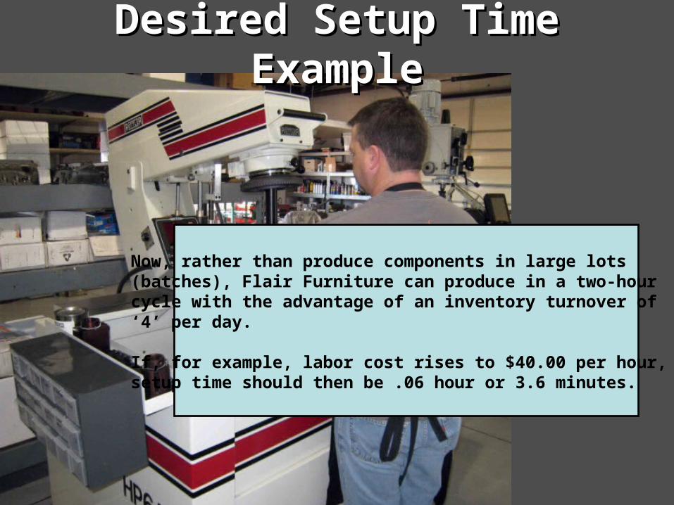
Desired Setup Time ExampleDesired Setup Time Example
Now, rather than produce components in large lots (batches), Flair Furniture can produce in a two-hour cycle with the advantage of an inventory turnover of ‘4’ per day.
If, for example, labor cost rises to $40.00 per hour, setup time should then be .06 hour or 3.6 minutes.
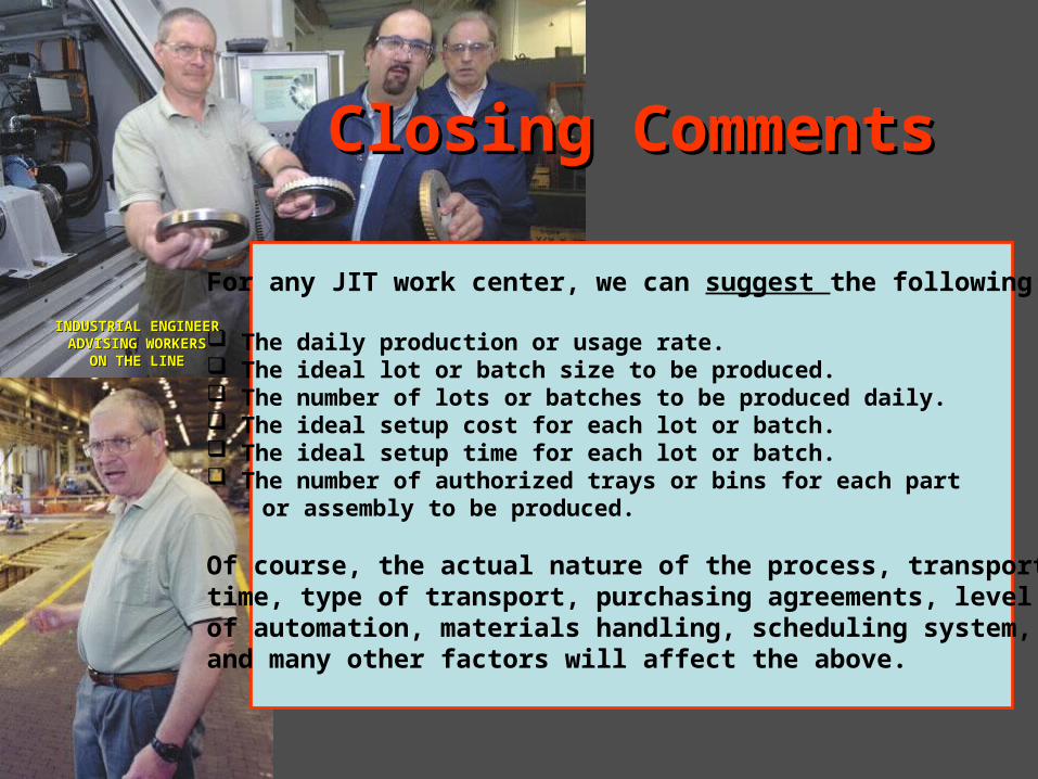
Closing CommentsClosing Comments
For any JIT work center, we can suggest the following:
The daily production or usage rate. The ideal lot or batch size to be produced. The number of lots or batches to be produced daily. The ideal setup cost for each lot or batch. The ideal setup time for each lot or batch. The number of authorized trays or bins for each part or assembly to be produced.
Of course, the actual nature of the process, transport time, type of transport, purchasing agreements, levelof automation, materials handling, scheduling system, and many other factors will affect the above.
INDUSTRIAL ENGINEERINDUSTRIAL ENGINEERADVISING WORKERSADVISING WORKERS
ON THE LINEON THE LINE

Successful JIT SystemsSuccessful JIT SystemsPATIENCEPATIENCE
5 to 15 years could pass before required changes to the production system, employees’ work, corporate philosophy, and work culture materialize. Inventories should be reduced slowly while making reductions in setup time, batch sizes, defects, and machine breakdowns.
That said, inventory reductions of 20% to 40% and productivity improvements of 5% to 10% annually for each of the first three years are common!

Successful JIT SystemsSuccessful JIT SystemsCUSTOMIZED IMPLEMENTATIONCUSTOMIZED IMPLEMENTATION
Every firm has a different level of experience and sophistication with regard to quality management, setup methods, job design, and maintenance.
Accordingly, the problems exposed by inventory reduction will vary.
The firm would be wise to wait for the most press- ing problems to appear and then respond to them quickly, rather than establishing its improvement programs in advance.

Successful JIT SystemsSuccessful JIT SystemsFLEXIBILITYFLEXIBILITY
There are occasions when product demand rises unexpectedly, and JIT will need to respond by in- creasing inventories temporarily. This can be done by simply increasing the num- ber of production and move cards for a product, or temporarily abandoning JIT before a seasonal surge in product demand so that inventory stock- piles can be built.

Successful JIT SystemsSuccessful JIT SystemsEXCESS CAPACITYEXCESS CAPACITY
JIT systems function best when they are designed to operate routinely at 80% to 90% of capacity, in turn, allowing production to accelerate when de- mand surges.
This also makes it possible to temporarily halt pro- duction immediately to correct quality problems. This also gives employees time to experiment with, and test improvements to the process, which will enhance productivity and capacity over time.

The “Just-for-You” SystemThe “Just-for-You” SystemJIT – “McDonald’s Style”
Trays for beef and fish patties are called universal holding cabinets and their number changes from hour to hour based on computer-forecasted de- mand.
Production cards have been superceded by closed- circuit television that relays orders received at the front counter to the backroom operation.
Setup times for patty cooking and bun warming have been slashed to seconds using equipment designed and produced by McDonald’s operations researchers and industrial engineers.

JIT at Federal Signal CorporationJIT at Federal Signal Corporation
Computer-controlled machinery mounted on rollers ( zero setup times & flexibility )
Workers responsible for their own setups, maintenance, quality control inspections, housekeeping, and assis- tance to others ( open job descriptions )
Morning classes to learn new product assembly steps.
Engineers on shop floor are workers’ technical resource.
Production problems receive a quick-fix on the line until a permanent solution is found at the workers’ regularly- scheduled quality circle meeting.

Just-in-Time SystemsJust-in-Time Systems
Applied Management Science for Decision Making, 1e Applied Management Science for Decision Making, 1e © 2012 Pearson Prentice-Hall, Inc. Philip A. Vaccaro , PhD© 2012 Pearson Prentice-Hall, Inc. Philip A. Vaccaro , PhD


![Submitted: Problems: Time to be settled. · authors [1,2] impute it to a ‘‘learning curve phenomenon’’, which frequently occurs after the introduction of any new procedure](https://img.dokumen.tips/doc/110x75/5faaff3e0bc2b86be23f54d5/submitted-problems-time-to-be-authors-12-impute-it-to-a-aalearning-curve.jpg)