© Goodwin, Graebe, Salgado, Prentice Hall 2000 Chapter 21 Exploiting SISO Techniques in MIMO Control

© Goodwin, Graebe, Salgado , Prentice Hall 2000Chapter 21

Chapter 21

Exploiting SISO Techniques in Exploiting SISO Techniques in MIMO ControlMIMO Control


In the case of SISO control, we found that one could use a wide variety of synthesis methods. Some of these carry over directly to the MIMO case. However, there are several complexities that arise in MIMO situations. For this reason, it is often desirable to use synthesis procedures that are in some sense automated. This will be the subject of the next few chapters. However, before we delve into the full complexity of MIMO design, it is appropriate that we pause to see when, if ever, SISO techniques can be applied to MIMO problems directly.


We will study

decentralized control as a mechanism for directly exploiting SISO methods in a MIMO setting

robustness issues associated with decentralized control.


Completely Decentralized Control

Before we consider a fully interacting multivariable design, it is often useful to check on whether a completely decentralized design can achieve the desired performance objectives. When applicable, the advantage of a completely decentralized controller, compared to a full MIMO controller, is that it is simpler to understand, is easier to maintain, and can be enhanced in a straightforward fashion (in the case of a plant upgrade).


Readers having previous exposure to practical control will realize that a substantial proportion of real-world systems will utilize decentralized architectures. Thus, one is led to ask the question, is there ever a situation in which decentralized control will not yield a satisfactory solution? We will present several real-world examples later in Chapter 22 that require MIMO thinking to get a satisfactory solution. As a textbook example of where decentralized control can break down, consider the following MIMO example.


Example 21.1

Consider a two-input, two-output plant having the transfer function


Let us say that k12 and k21 depend on the operating point (a common situation, in practice).

Operating point 1 (k12 = k21 = 0)

Clearly, there is no interaction at this operating point.

Thus, we can safely design two SISO controllers. To be specific, say we aim for the following complementary sensitivities:


The corresponding controller transfer functions are C1(s) and C2(s), where

The two independent loops perform as predicted by the choice of complementary sensitivities.


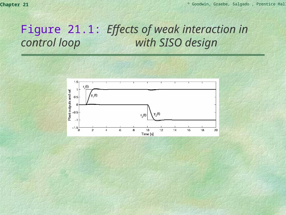
Operating point 2 (k12 = k21 = 0.1)

We leave the controller as previously designed for operating point 1. We apply a unit step in the reference for output 1 at t = 1 and a unit step in the reference for output 2 at t = 10. The closed-loop response is shown on the next slide. These results would probably be considered very acceptable, even though the effects of coupling are now evident in the response.


Figure 21.1: Effects of weak interaction in control loop with SISO design


Operating point 3 (k12 = -1, k21 = 0.5)

With the same controllers and for the same test as used at operating point 2, we obtain the results on the next slide.

We see that a change in the reference in one loop now affects the output in the other loop significantly.


Figure 21.2: Effects of strong interaction in control loops with SISO design


Operating point 4 (k12 = -2, k21 = -1)

Now a simulation with the same reference signals indicates that the whole system becomes unstable. We see that the original SISO design has become unacceptable at this final operating point.


Pairing of Inputs and Outputs

If one is to use a decentralized architecture, then one needs to pair the inputs and outputs. In the case of an m m plant transfer function, there are m! possible pairings. However, physical insight can often be used to suggest sensible pairings.


Relative Gain Array

One method that can be used to suggest pairings is a quantity known as the Relative Gain Array (RGA). For a system with matrix transfer function Go(s), the RGA is defined as a matrix with the ijth element

where [Go(0)]ij and [Go-1(0)]ij denote the ijth element of

the plant d.c. gain and the jith element of the inverse of the d.c. gain matrix respectively.


Note that [Go(0)]ij corresponds to the d.c. gain from the ith input, ui, to the jth output, yj, while the rest of the inputs, ul for l {1, 2, …, i-1, i+1, …, m} are kept constant. Also [Go

-1]ij is the reciprocal of the d.c. gain from the ith input, ui, to the jth output, yj, while the rest of the outputs, yl for l {1, 2, …, j-1, j+1, …, m} are kept constant. Thus, the parameter ij provides an indication of how sensible it is to pair the ith input with the jth output.


One usually aims to pick pairings such that the diagonal entries of are large. One also tries to avoid pairings that result in negative diagonal entries in .


Example

Consider again the system

The RGA is then


For 1 > k12 > 0, 1 > k21 > 0, the RGA suggests the pairing (u1, y1), (u2, y2). We recall from our earlier study of this example that this pairing worked very well for k12 = k21 = 0.1 and quite acceptably for k12 = -1, k21 = 0.5. In the latter case, the RGA is


However, for k12 = -2, k21 = -1 we found that the centralized controller based on the pairing (u1, y1), (u2, y2) was actually unstable. The corresponding RGA in this case is

which indicates that we probably should have changed to the pairing (u1, y2), (u2, y1).


Example 21.3

Quadruple-tank apparatus.

Consider the quadruple-tank apparatus shown on the next two slides.




We recall from Chapter 20 that this system has an approximate transfer function,

The RGA for this system is


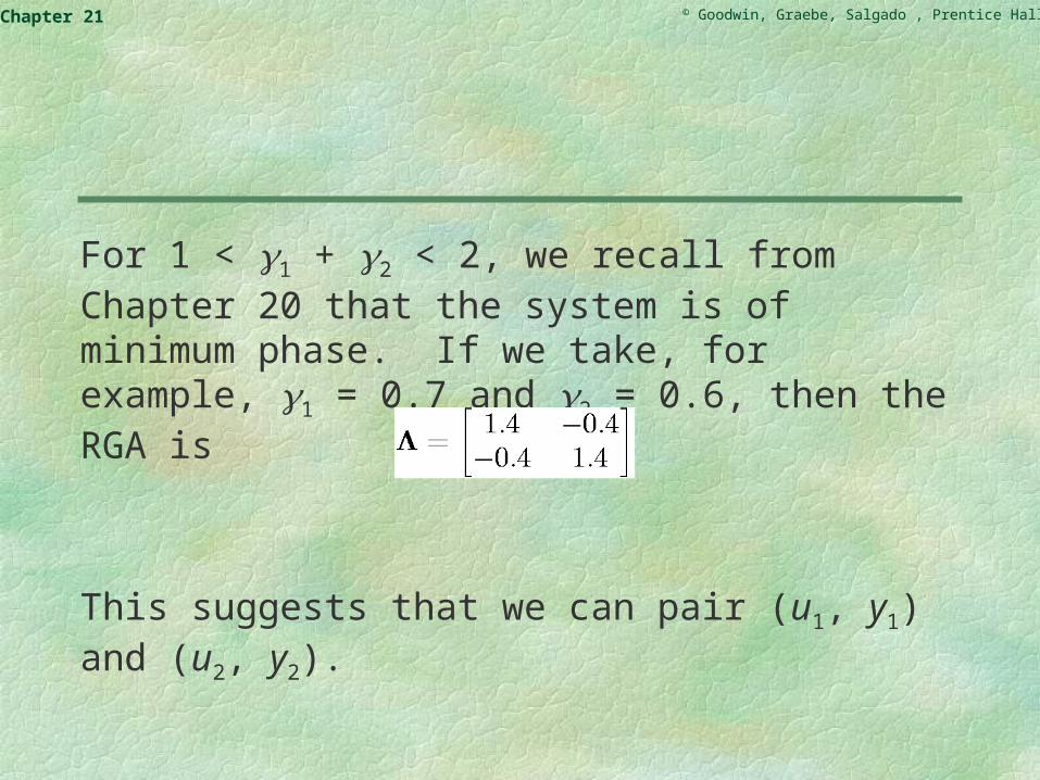
For 1 < 1 + 2 < 2, we recall from Chapter 20 that the system is of minimum phase. If we take, for example, 1 = 0.7 and 2 = 0.6, then the RGA is

This suggests that we can pair (u1, y1) and (u2, y2).


Because the system is of minimum phase, the design of a decentralized controller is relatively easy in this case. For example, the following decentralized controller gives the results shown on the next slide


Figure 21.3: Decentralized control of a minimum-phase four-tank system


For 0 < 1 + 2 < 1, we recall from Chapter 20 that the system is nonminimum phase. If we take, for example 1 = 0.43 and 2 = 0.34, then the system has a NMP zero at s = 0.0229, and the relative gain array becomes


This suggests that (y1, y2) should be commuted for the purposes of decentralized control,. This is physically reasonable, given the flow patterns produced in this case. This leads to a new RGA of


Note, however, that control will still be much harder than in the minimum-phase case. For example, the following decentralized controllers give the results shown on the next slide.


Figure 21.4: Decentralized control of a nonminimum-phase four-tank system


Robustness Issues in Decentralized Control

One way to carry out a decentralized control design is to use a diagonal nominal model. The off-diagonal terms then represent under-modelling, in the terminology of Chapter 3.


Thus, say we have a model Go(s), then the nominal model for decentralized control could be chosen as

and the additive model error would be

With this as a background, we can employ the robustness checks described in Chapter 20. We recall that a sufficient condition for robust stability is

where is the maximum singular value of ))()(( 1 jj oTG

).()(1 jj oTG


Example



In this case, the various matrices arising in the centralized design are


The singular values, in this case, are simply the magnitudes of the two off-diagonal elements. These are plotted on the next slide for normalized values k12 = k21 = 1.


Figure 21.5: Singular Values of G1(j)To(j)


We see that a sufficient condition for robust stability of the decentralized control, with the pairing (u1, y1), (u2, y2), is that |k12| < 1 and |k21| < 1. Observe that this is conservative, but consistent with the performance results presented earlier.


Example

Consider a MIMO system with

We first observe that the RGA for the nominal model Go(s) is given by


This value of the RGA might lead to the hypothesis that a correct pairing of inputs and outputs has been made and that the interaction is weak. We thus proceed to do a decentralized design leading to a diagonal controller C(s) to achieve a complementary sensitivity To(s), where


However, this controller, when applied to control the full plant G(s), leads to closed-loop poles located at -6.00, -2.49 ± j4.69, 0.23 ± j1.36, and -0.50 - an unstable closed loop !

The lack of robustness in this example can be traced to the fact that the required closed-loop bandwidth includes a frequency range where the off-diagonal frequency response is significant.


Feedforward Action in Decentralized Control

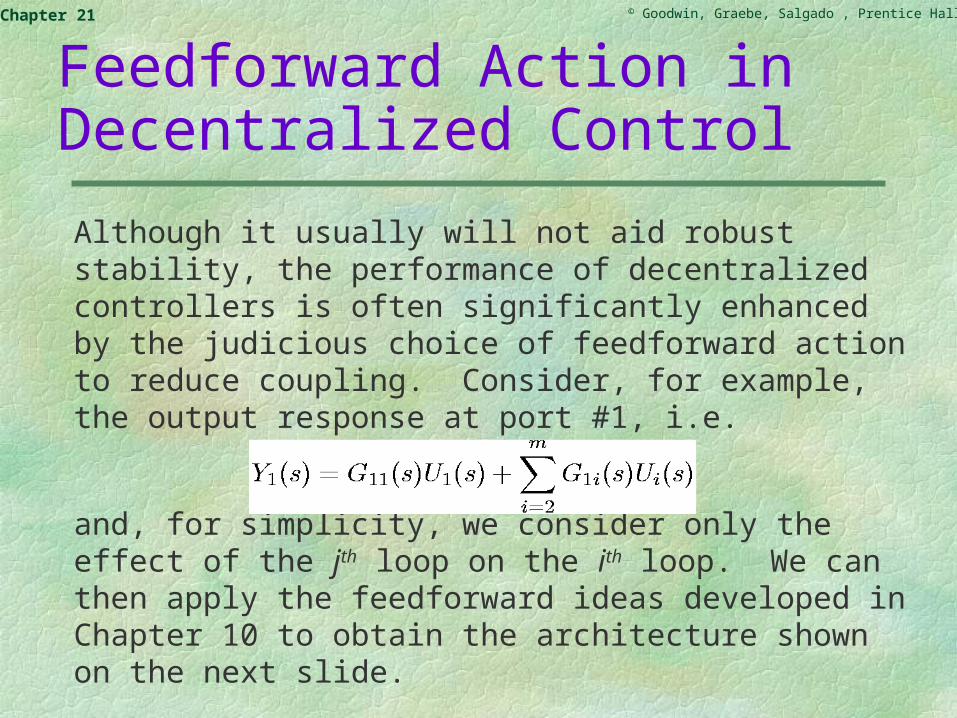
Although it usually will not aid robust stability, the performance of decentralized controllers is often significantly enhanced by the judicious choice of feedforward action to reduce coupling. Consider, for example, the output response at port #1, i.e.

and, for simplicity, we consider only the effect of the jth loop on the ith loop. We can then apply the feedforward ideas developed in Chapter 10 to obtain the architecture shown on the next slide.


Figure 21.6: Feedforward action in decentralized control


The feedforward gain should be chosen in such a way that the coupling from the jth loop to the ith loop is compensated in a particular, problem-dependent frequency band [0 ff] - i.e.

This can also be written as

from which we observe the necessity to build an inverse. Hence all of the issues associated with building inverses discussed in earlier chapters arise again.

)( sG jiff


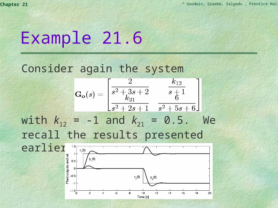
Example 21.6


with k12 = -1 and k21 = 0.5. We recall the results presented earlier for this case.


We see that there is little coupling from the first to the second loop, but relatively strong coupling from the second to the first loop. This suggests that feedforward from the second input to the first loop may be beneficial. To illustrate, we choose to completely compensate the coupling at d.c., i.e. is chosen to be a constant , satisfying

)( sG jiff

)( sG jiff

)( sG jiff


The resulting modified MIMO system can be seen to be modeled by

where


The RGA is now = diag(1, 1) and when we redesign the decentralized controller, we obtain the results presented on the next slide.


Figure 21.7: Performance of a MIMO decentralized control loop with interaction feedforward


The above examples indicate that a little coupling introduced into the controller can be quite helpful. This, however, raises the question of how we can systematically design coupled controllers that rigorously take into account multivariable interaction. This motivates us to study the latter topic, which will be taken up in the next chapter. Before ending this chapter, we investigate whether there exist simple ways of converting an inherently MIMO problem to a set of SISO problems.


Converting MIMO problems to SISO Problems

Many MIMO problems can be modified so that decentralized control becomes a more viable (or attractive) option. For example, one can sometimes use a precompensator to turn the resultant system into a more nearly diagonal transfer function.


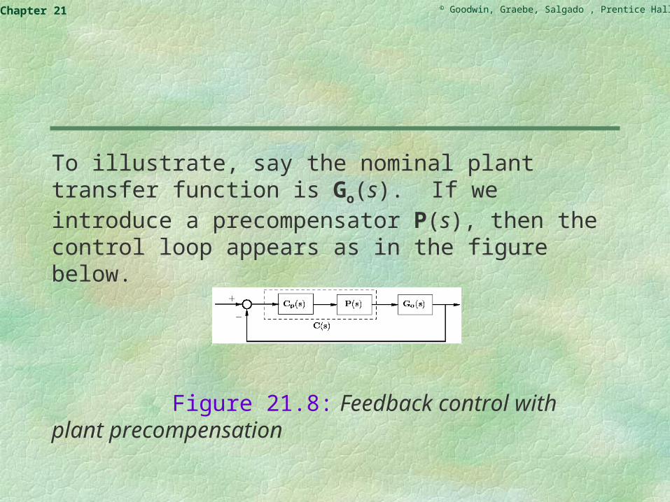
To illustrate, say the nominal plant transfer function is Go(s). If we introduce a precompensator P(s), then the control loop appears as in the figure below.

Figure 21.8: Feedback control with plant precompensation


The design of Cp(s) can then be based on the equivalent plant.


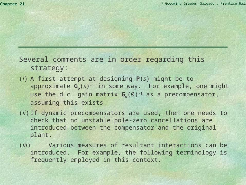
Several comments are in order regarding this strategy:

(i) A first attempt at designing P(s) might be to approximate Go(s)-

1 in some way. For example, one might use the d.c. gain matrix Go(0)-1 as a precompensator, assuming this exists.

(ii) If dynamic precompensators are used, then one needs to check that no unstable pole-zero cancellations are introduced between the compensator and the original plant.

(iii) Various measures of resultant interactions can be introduced. For example, the following terminology is frequently employed in this context.


Dynamically decoupled

Dynamically decoupled: Here, every output depends on one and only one input. The transfer-function matrix H(s) is diagonal for all s. In this case, the problem reduces to separate SISO control loops.

Band-decoupled and statically decoupled systems: When the transfer-function matrix H(j) is diagonal only in a finite frequency band, we say that the system is decoupled in that band. In particular, we will say, when H(0) is diagonal, that the system is statically decoupled.


Triangularly coupled systems: A system is triangularly coupled when the inputs and outputs can be ordered in such a way that the transfer-function matrix H(s) is either upper or lower triangular, for all s. The coupling is then hierarchical.


Industrial Case Study (Strip Flatness Control)

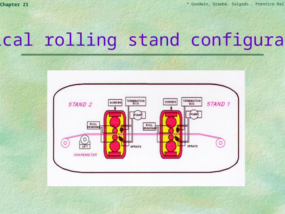
An an illustration of the use of simple precompensators to convert a MIMO problem into one in which SISO techniques can be employed, we consider the problem of strip flatness control in rolling mills. Actually, very similar issues arise in many other problems including paper making and plastic extrusion.

The next slide shows a typical rolling stand configuration.


Typical rolling stand configuration


What is flatness in a Rolling Mill?

If rolling results in a nonuniform reduction of the strip thickness across the strip width, then a residual stress will be created, and buckling of the final product may occur. A practical difficulty is that flatness defects can be pulled out by the applied strip tensions, so that they are not visible to the mill operator. However, the buckling will become apparent as the coil is unwound or after it is slit or cut to length in subsequent processing operations.


Source of Flatness Problems

There are several sources of flatness problems, including the following:

roll thermal cambers incoming fed disturbances (profile, hardness, thickness) transverse temperature gradients roll stack deflections incorrect ground roll cambers roll wear inappropriate mill setup (reduction, tension, force, roll bending) lubrication effects.


On the other hand, there are strong economic motives to control strip flatness, including the following:

improved yield of prime-quality strip increased throughput, due to faster permissible acceleration,

reduced threading delay, and higher rolling speed on shape-critical products

more efficient recovery and operation on such downstream units as annealing and continuous-process lines

reduced reprocessing of material on tension-leveling lines or temper-rolling mills.


Control Options

In this context, there are several control options to achieve improved flatness. These include roll tilt, roll bending, and cooling sprays. These typically can be separated by preprocessing the measured shape. Here, we will focus on a particular aspect of the cooling spray option. Note that flatness defects can be measured across the strip by using a special instrument called a Shape Meter. A typical control configuration is shown on the next slide.


Figure 21.9: Typical flatness-control set-up for rolling mill


In this configuration, numerous cooling sprays are located across the roll, and the flow through each spray is controlled by a valve. The cool water sprayed onto the roll reduces the thermal expansion. The interesting thing is that each spray affects a large section of the roll, not just the section directly beneath it. This leads to an interactive MIMO system, rather than a series of decoupled SISO systems.


The thermal properties of the roll can be modeled using basic laws of physics. This leads to a partial differential equation, however, this can be discretized to give a finite dimenional model. Such a model can then be used as a calibration model to test control system design strategies.

The main components of the heat flow inside a typical roll are shown on the next slide.


Internal roll heat flows


For the purpose of control system design, it suffices to use a simpler model. Such a model can be developed by approximating the observed behavior of the more complex calibration model. A key feature of the observed behavior is that a single cooling spray (one of the actuators) effects the radial diameter of the roll and hence the measured strip shape over a extended spatial area. This is diagrammatically shown on the next slide.


Action of single spray

Effect of a single spray on roll diameter


Based on the above discussion, a simplified model for this system (ignoring nonlinear heat-transfer effects, etc.) is shown in the block diagram on the next slide, where U denotes a vector of spray valve positions and Y denotes the roll-thickness vector. (The lines indicate vectors rather than single signals).


Figure 21.10: Simplified flatness-control feedback loop


The sprays affect the roll in a roughly exponential fashion as described by the matrix M:

The parameter represents the level of interactivity in the system and is determined by the number of sprays present and how close together they are.


An interesting thing about this simplified model is that the interaction is captured totally by the d.c. gain matrix M. This suggests that we could design an approximate precompensator by simply inverting this matrix. This leads to


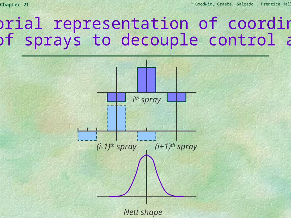
Using this matrix to decouple the system has a nice physical interpretation. Namely, it amounts to turning off surrounding sprays when a spray is turned on. This makes sense physically since we are preventing the spread of the cooling effect by use of adjacent sprays. The essential idea of the decoupling control strategy is shown on the next slide.


Pictorial representation of coordinated use of sprays to decouple control action

Nett shape

ith spray

(i-1)th spray (i+1)th spray


In summary, we can (approximately) decouple the system simply by multiplying the control vector by the appropriate inverse. This set-up is shown in the block diagram on the next slide.


Figure 21.11: Flatness control with precompensation


The nominal decoupled system then becomes simply With this new model, the controller can be

designed by using SISO methods. For example a set of simple PI controllers linking each shape meter with the corresponding spray would seem to suffice. (We assume that the shape meters measure the shape of the rolls perfectly).

This idea is routinely used in this particular application and leads to excellent results. (Of course, the practical problem has many other features that we leave aside so as not to distract from our key point here).

.)( )1(1 sdiagsH


Actually, control problems almost identical to the above can be found in many alternative industrial situations where there are longitudinal and traverse effects. Examples are paper making and plastic extrusion.


Strip flatness systems of the type (briefly) described here are available commercially. The following slides have been made from pamphlets describing a commercial system sold by Industrial Automation Services Pty. Ltd.

www.indauto.com.au






Impact of MIMO Controller


Summary

A fundamental decision in MIMO synthesis pertains to the choice of decentralized versus full MIMO control.

Completely decentralized control In completely decentralized control, the MIMO system is

approximated as a set of independent SISO systems

To do so, multivariable interactions are thought of as disturbances; this is an approximation, because the interactions involve feedback, whereas disturbance analysis actually presumes disturbances to be independent inputs.

When applicable, the advantage of completely decentralized control is that one can apply the simpler SISO theory.


Applicability of this approximation depends on the neglected interaction dynamics, which can be viewed as modelilng errors; robustness analysis can be applied to determine their impact.

Chances of success are increased by judiciously pairing inputs and outputs (for example, by using the Relative Gain Array, RGA) and by using feedforward.

Feedforward is often a very effective tool in MIMO problems.

Some MIMO problems can be better treated as SISO problems if a precompensator is first used.


There are several ways to quantify interactions in multivariable systems, including their structure and their strength.

Interactions can have a completely general structure (every input potentially affects every output) or display particular patterns, such as triangular or dominant diagonal; they can also display frequency-dependent patterns, such as being statistically decoupled or band-decoupled.

The lower the strength of interaction, the more nearly a system behaves like a set of independent systems that can be analyzed and controlled separately.


Weak coupling can be due to the nature of the interacting dynamics or to a separation in frequency range or time scale.

The stronger is the interaction, the more important it becomes to view the multi-input multi-output system and its interactions as a whole.

Compared to the SISO techniques discussed so far, viewing the MIMO systems and its interactions as a whole requires generalized synthesis and design techniques and insight. These will be the topics of the following two chapters.

Documents

© Goodwin, Graebe, Salgado, Prentice Hall 2000 Chapter 21 Exploiting SISO Techniques in MIMO Control