© Goodwin, Graebe, Salgado, Prentice Hall 2000 Chapter 18 Synthesis via State Space Methods

© Goodwin, Graebe, Salgado , Prentice Hall 2000Chapter 18

Chapter 18

Synthesis via State Space Synthesis via State Space MethodsMethods


Here, we will give a state space interpretation to many of the results described earlier. In a sense, this will duplicate the earlier work. Our reason for doing so, however, is to gain additional insight into linear-feedback systems. Also, it will turn out that the alternative state space formulation carries over more naturally to the multivariable case.


Results to be presented include pole assignment by state-variable feedback

design of observers to reconstruct missing states from available output measurements

combining state feedback with an observer

transfer-function interpretation

dealing with disturbances in state-variable feedback

reinterpretation of the affine parameterization of all stabilizing controllers.


Pole Assignment by State Feedback

We begin by examining the problem of closed-loop pole assignment. For the moment, we make a simplifying assumption that all of the system states are measured. We will remove this assumption later. We will also assume that the system is completely controllable. The following result then shows that the closed-loop poles of the system can be arbitrarily assigned by feeding back the state through a suitably chosen constant-gain vector.


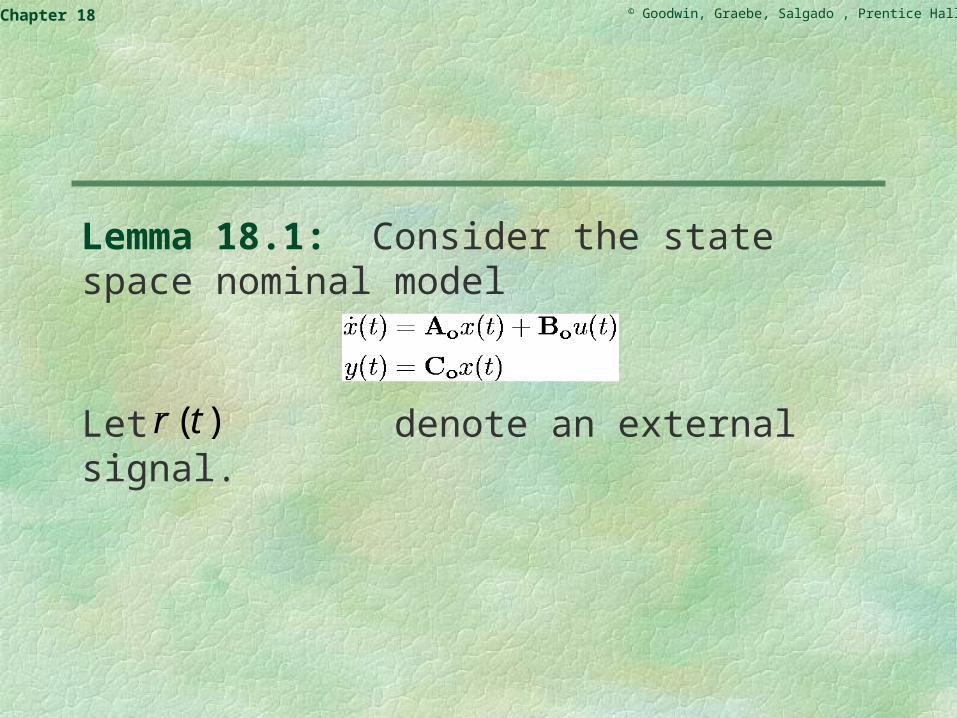
Lemma 18.1: Consider the state space nominal model

Let denote an external signal.)( tr


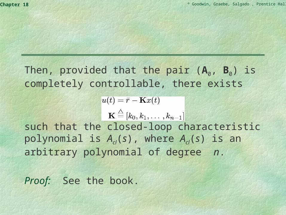
Then, provided that the pair (A0, B0) is completely controllable, there exists

such that the closed-loop characteristic polynomial is Acl(s), where Acl(s) is an arbitrary polynomial of degree n.

Proof: See the book.


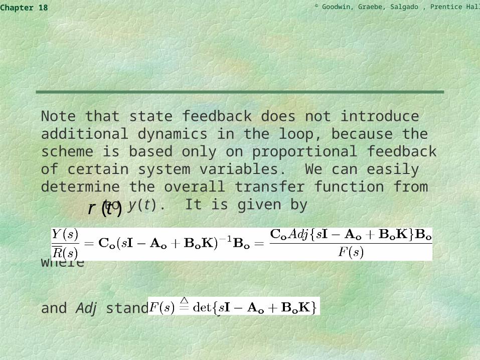
Note that state feedback does not introduce additional dynamics in the loop, because the scheme is based only on proportional feedback of certain system variables. We can easily determine the overall transfer function from to y(t). It is given by

where

and Adj stands for adjoint matrices.

)( tr


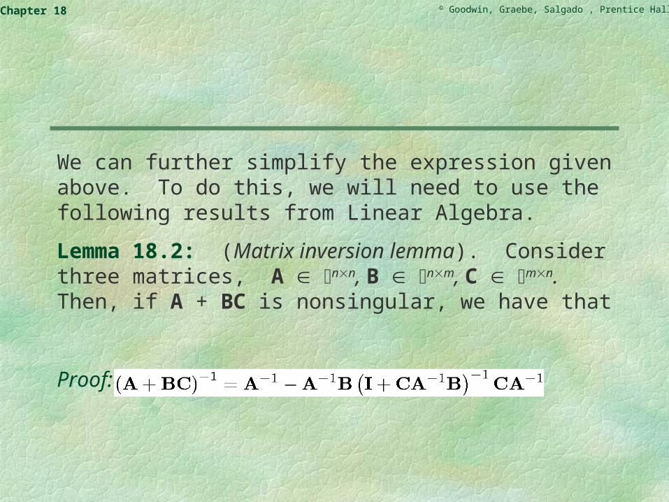
We can further simplify the expression given above. To do this, we will need to use the following results from Linear Algebra.

Lemma 18.2: (Matrix inversion lemma). Consider three matrices, A nn, B nm, C mn. Then, if A + BC is nonsingular, we have that



In the case for which B = g n and CT = h n, the above result becomes


Lemma 18.3: Given a matrix W nn and a pair of arbitrary vectors 1 n and 2 n, then provided that W and are nonsingular,


,21TW


Application of Lemma 18.3 to equation

leads to

we then see that the right-hand side of the above expression is the numerator B0(s) of the nominal model, G0(s). Hence, state feedback assigns the closed-loop poles to a prescribed position, while the zeros in the overall transfer function remain the same as those of the plant model.


State feedback encompasses the essence of many fundamental ideas in control design and lies at the core of many design strategies. However, this approach requires that all states be measured. In most cases, this is an unrealistic requirement. For that reason, the idea of observers is introduced next, as a mechanism for estimating the states from the available measurements.


Observers

Consider again the state space model

A general linear observer then takes the form

where the matrix J is called the observer gain and is the state estimate.)(ˆ tx


The term

is known as the innovation process. For nonzero J v(t) represents the feedback error between the observation and the predicted model output.


The following result shows how the observer gain J can be chosen such that the error, defined as

can be made to decay at any desired rate.

)(~ tx


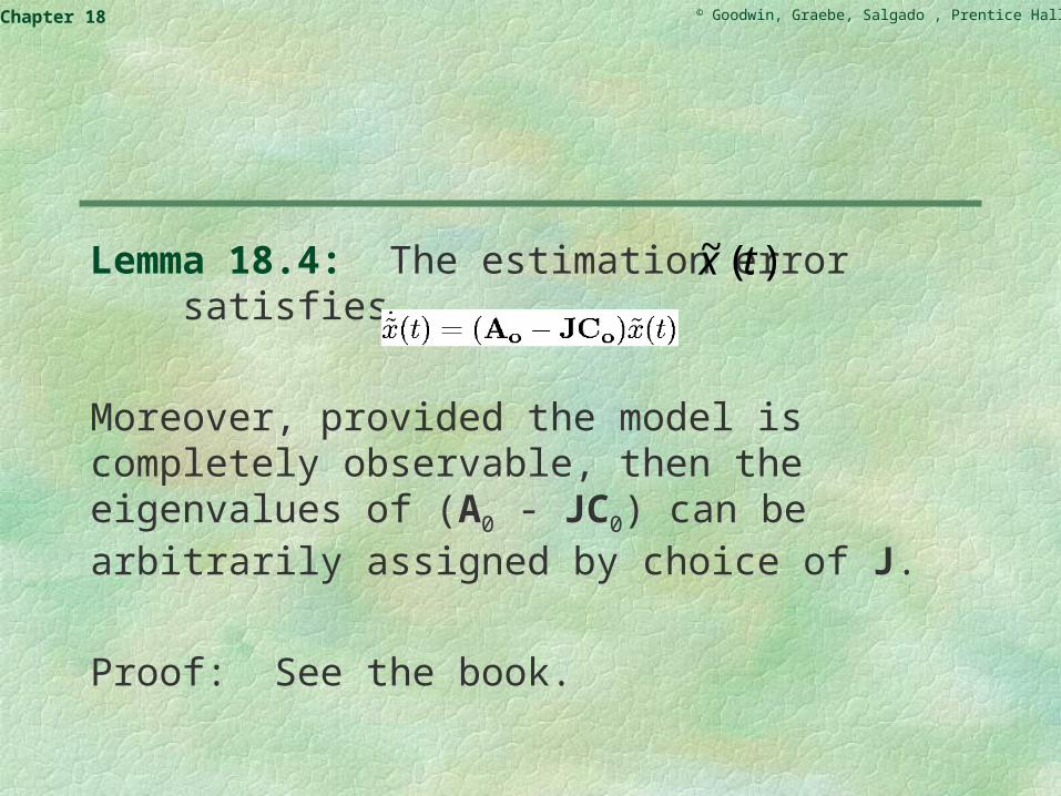
Lemma 18.4: The estimation error satisfies

Moreover, provided the model is completely observable, then the eigenvalues of (A0 - JC0) can be arbitrarily assigned by choice of J.


)(~ tx


Example 18.1: Tank-level estimation

As a simple application of a linear observer to estimate states, we consider the problem of two coupled tanks in which only the height of the liquid in the second tank is actually measured but where we are also interested in estimating the height of the liquid in the first tank. We will design a virtual sensor for this task.

A photograph is given on the next slide.


Coupled Tanks Apparatus


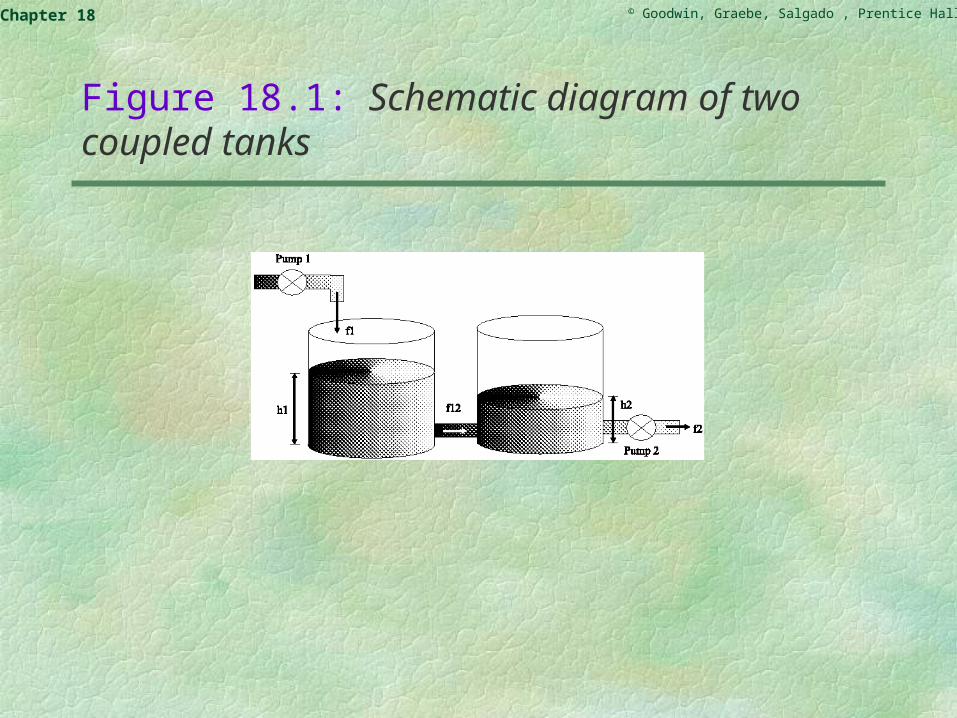
Figure 18.1: Schematic diagram of two coupled tanks


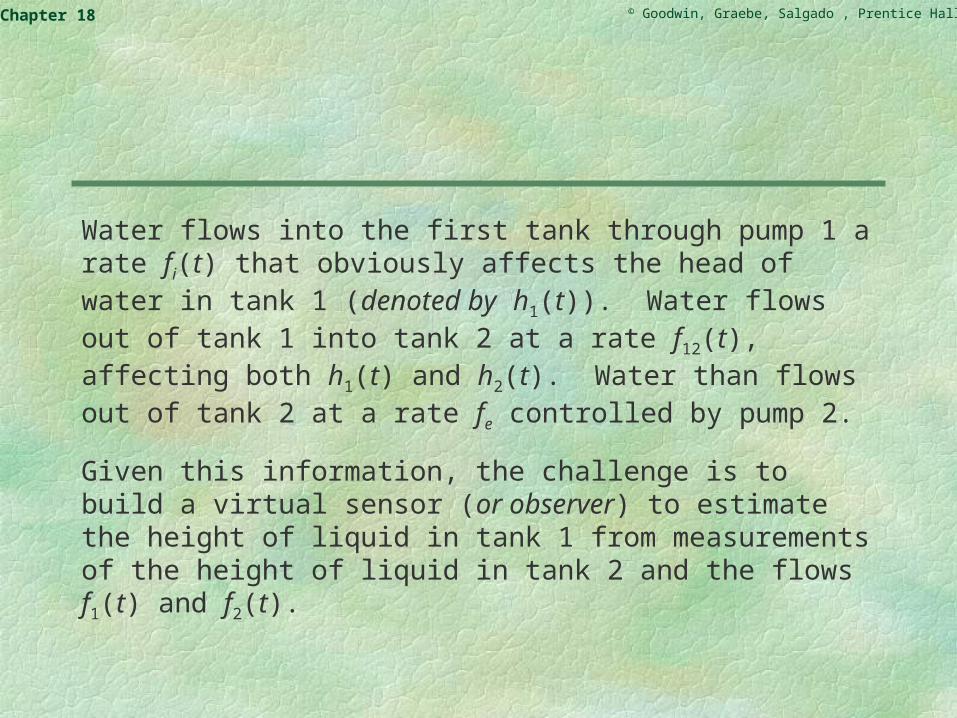
Water flows into the first tank through pump 1 a rate fi(t) that obviously affects the head of water in tank 1 (denoted by h1(t)). Water flows out of tank 1 into tank 2 at a rate f12(t), affecting both h1(t) and h2(t). Water than flows out of tank 2 at a rate fe controlled by pump 2.

Given this information, the challenge is to build a virtual sensor (or observer) to estimate the height of liquid in tank 1 from measurements of the height of liquid in tank 2 and the flows f1(t) and f2(t).


Before we continue with the observer design, we first make a model of the system. The height of liquid in tank 1 can be described by the equation

Similarly, h2(t) is described by

The flow between the two tanks can be approximated by the free-fall velocity for the difference in height between the two tanks:


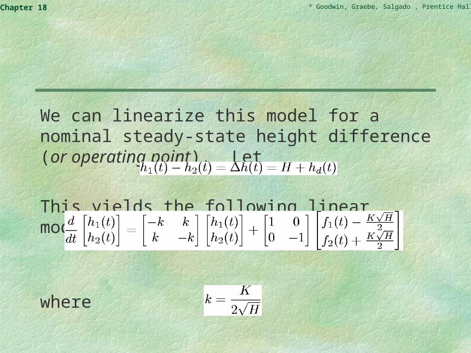
We can linearize this model for a nominal steady-state height difference (or operating point). Let

This yields the following linear model:

where


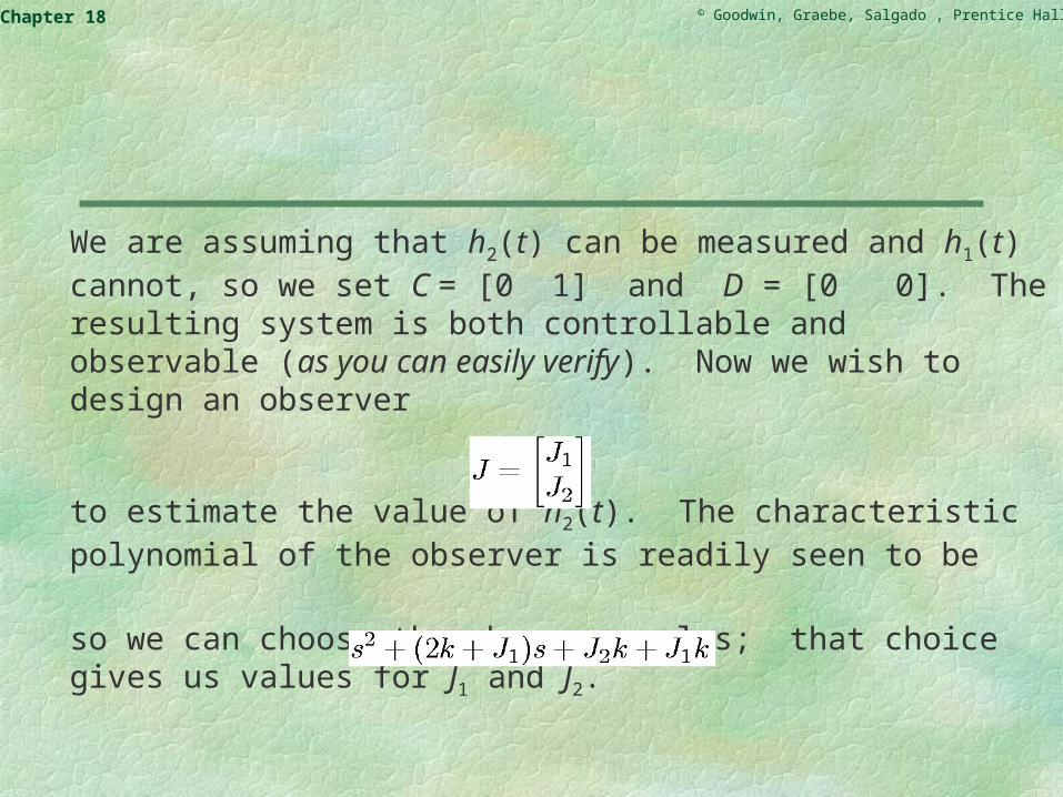
We are assuming that h2(t) can be measured and h1(t) cannot, so we set C = [0 1] and D = [0 0]. The resulting system is both controllable and observable (as you can easily verify). Now we wish to design an observer

to estimate the value of h2(t). The characteristic polynomial of the observer is readily seen to be

so we can choose the observer poles; that choice gives us values for J1 and J2.


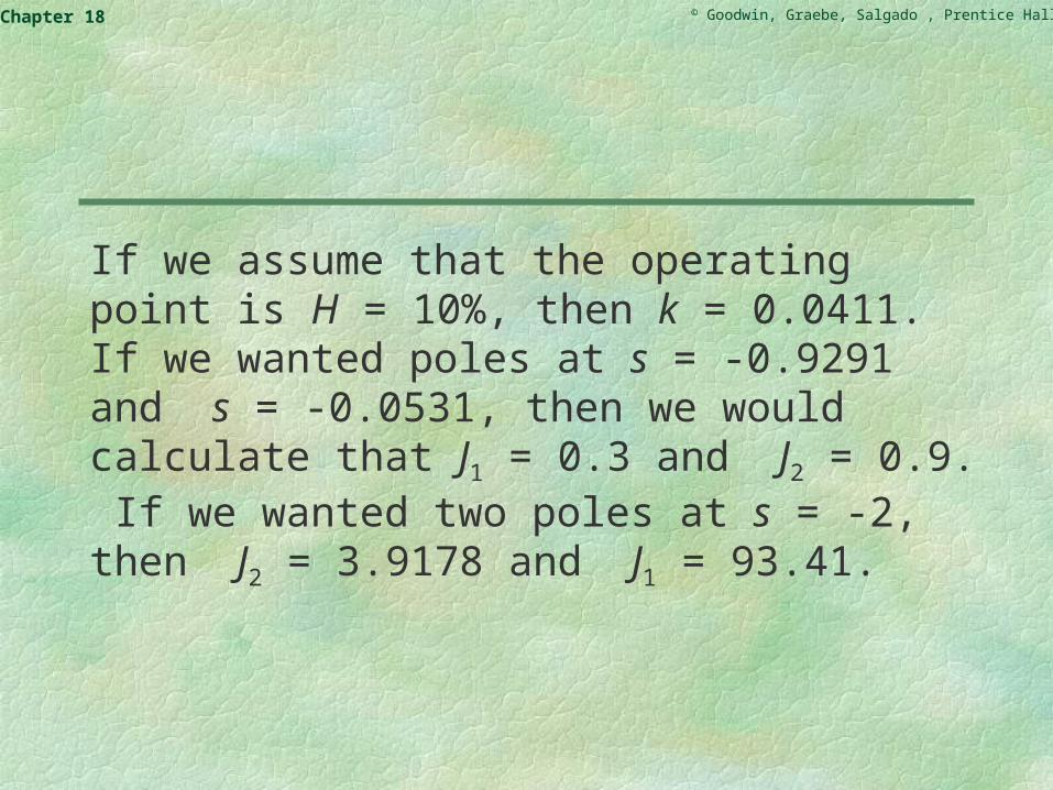
If we assume that the operating point is H = 10%, then k = 0.0411. If we wanted poles at s = -0.9291 and s = -0.0531, then we would calculate that J1 = 0.3 and J2 = 0.9. If we wanted two poles at s = -2, then J2 = 3.9178 and J1 = 93.41.


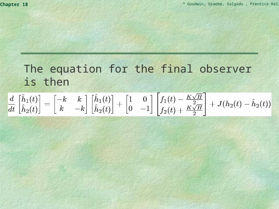
The equation for the final observer is then


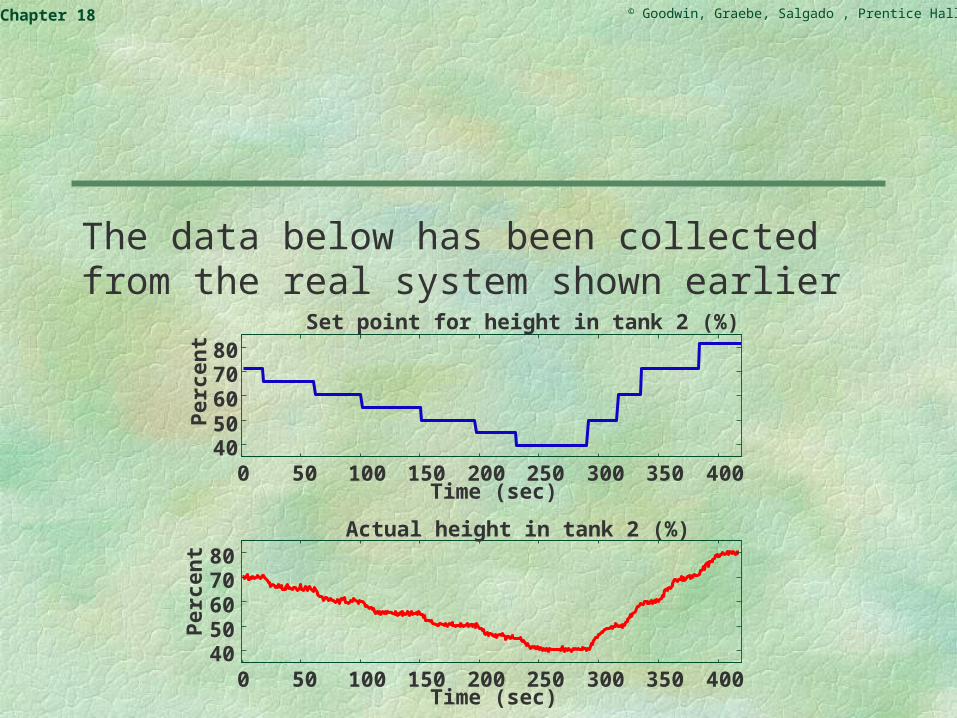
The data below has been collected from the real system shown earlier

0 50 100 150 200 250 300 350 4004050607080

Set point for height in tank 2 (%)

Time (sec)

Per

cen

t

0 50 100 150 200 250 300 350 4004050607080

Actual height in tank 2 (%)

Time (sec)

Per

cen

t


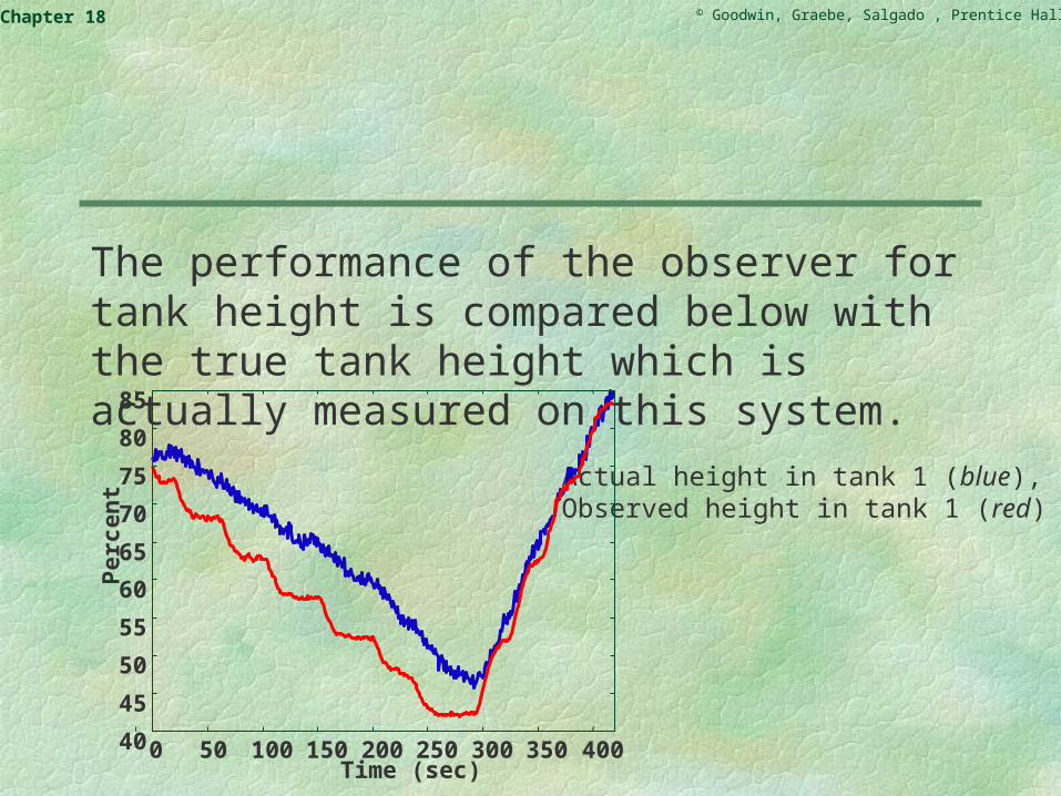
The performance of the observer for tank height is compared below with the true tank height which is actually measured on this system.

Actual height in tank 1 (blue), Observed height in tank 1 (red)

0 50 100 150 200 250 300 350 40040

45

50

55

60

65

70

75

80

85

Time (sec)

Per

cen

t


Combining State Feedback with an Observer

A reasonable conjecture arising from the last two sections is that it would be a good idea, in the presence of unmeasurable states, to proceed by estimating these states via an observer and then to complete the feedback control strategy by feeding back these estimates in lieu of the true states. Such a strategy is indeed very appealing, because it separates the task of observer design from that of controller design. A-priori, however, it is not clear how the observer poles and the state feedback interact. The following theorem shows that the resultant closed-loop poles are the combination of the observer and the state-feedback poles.


Separation Theorem

Theorem 18.1: (Separation theorem). Consider the state space model and assume that it is completely controllable and completely observable. Consider also an associated observer and state-variable feedback, where the state estimates are used in lieu of the true states:


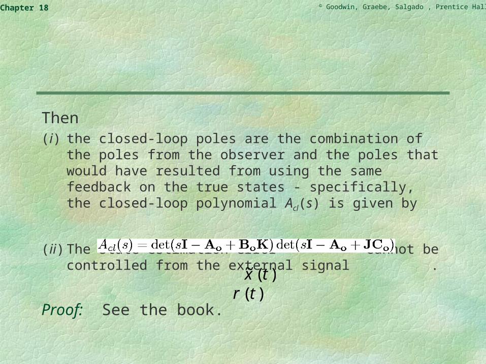
Then(i) the closed-loop poles are the combination of the poles from

the observer and the poles that would have resulted from using the same feedback on the true states - specifically, the closed-loop polynomial Acl(s) is given by

(ii) The state-estimation error cannot be controlled from the external signal .


)(~ tx)( tr


The above theorem makes a very compelling case for the use of state-estimate feedback. However, the reader is cautioned that the location of closed-loop poles is only one among many factors that come into control-system design. Indeed, we shall see later that state-estimate feedback is not a panacea. Indeed it is subject to the same issues of sensitivity to disturbances, model errors, etc. as all feedback solutions. In particular, all of the schemes turn out to be essentially identical.


Transfer-Function Interpretations

In the material presented above, we have developed a seemingly different approach to SISO linear control-systems synthesis. This could leave the reader wondering what the connection is between this and the transfer-function ideas presented earlier. We next show that these two methods are actually different ways of expressing the same result.


Transfer-Function Form of Observer

We first give a transfer-function interpretation to the observer. We recall that the state space observer takes the form

where J is the observer gain and is the state estimate.

)(ˆ tx


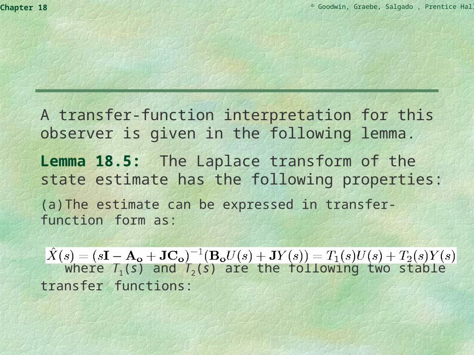
A transfer-function interpretation for this observer is given in the following lemma.

Lemma 18.5: The Laplace transform of the state estimate has the following properties:

(a) The estimate can be expressed in transfer-function form as:

where T1(s) and T2(s) are the following two stable transfer functions:



(b) The estimate is related to the input and initial conditions by

where f0(s) is a polynomial vector in s with coefficients depending linearly on the initial conditions of the error

(c) The estimate is unbiased in the sense that

where G0(s) is the nominal plant model.


).(~ tx


Transfer-Function Form of State-Estimate Feedback

We next give a transfer-function interpretation to the interconnection of an observer with state-variable feedback. The key result is described in the following lemma.

Lemma 18.6:(a) The state-estimate feedback law

can be expressed in transfer-function form as

where E(s) is the polynomial defined previously.


In the above feedback law

where K is the feedback gain and J is the observer gain.


(b) The closed-loop characteristic polynomial is


(c) The transfer function from to Y(s) is given by

where B0(s) and A0(s) are the numerator and denominator of the nominal loop respectively. P(s) and L(s) are the polynomials defined above.

)( tR


The foregoing lemma shows that polynomial pole assignment and state-estimate feedback lead to the same result. Thus, the only difference is in the terms of implementation.


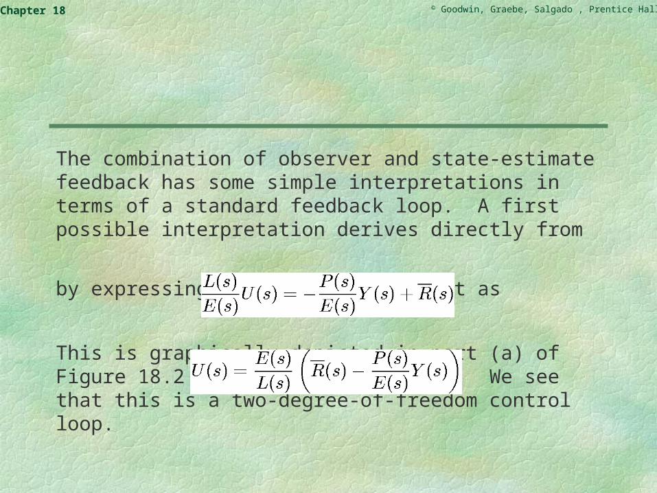
The combination of observer and state-estimate feedback has some simple interpretations in terms of a standard feedback loop. A first possible interpretation derives directly from

by expressing the controller output as

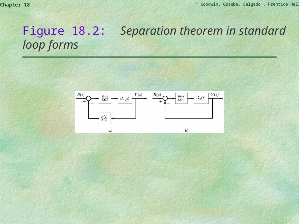
This is graphically depicted in part (a) of Figure 18.2 on the following slide. We see that this is a two-degree-of-freedom control loop.


Figure 18.2: Separation theorem in standard loop forms


A standard one-degree-of-freedom loop can be obtained if we generate from the loop reference r(t) as follows:

We then have

This corresponds to the one-degree-of-freedom loop shown in part (b) of Figure 18.2.

)( tr


Note that the feedback controller can be implemented as a system defined, in state space form, by the 4-tuple (A0 - JC0 - B0K, J, K, 0). (MATLAB provides a special command, reg, to obtain the transfer function form.)


Transfer Function for Innovation Process

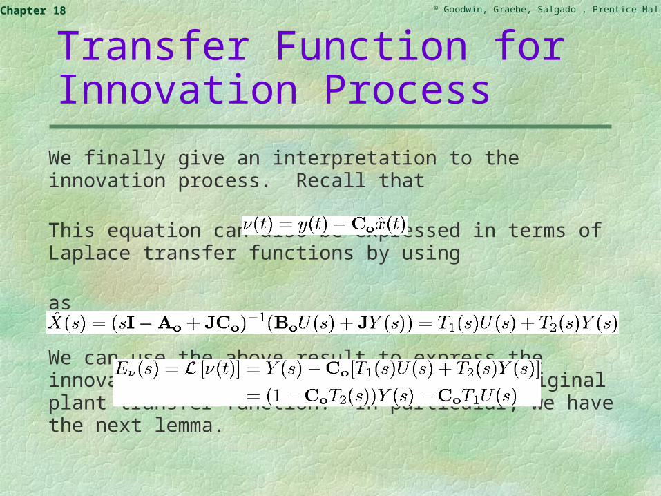
We finally give an interpretation to the innovation process. Recall that

This equation can also be expressed in terms of Laplace transfer functions by using

as

We can use the above result to express the innovation process v(t) in terms of the original plant transfer function. In particular, we have the next lemma.


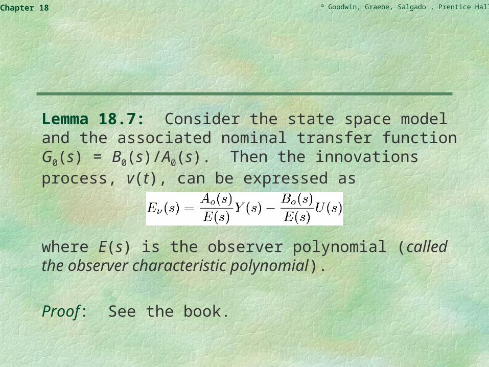
Lemma 18.7: Consider the state space model and the associated nominal transfer function G0(s) = B0(s)/A0(s). Then the innovations process, v(t), can be expressed as

where E(s) is the observer polynomial (called the observer characteristic polynomial).



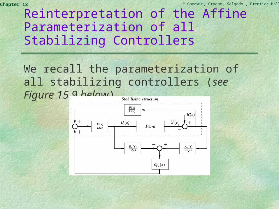
Reinterpretation of the Affine Parameterization of all Stabilizing Controllers

We recall the parameterization of all stabilizing controllers (see Figure 15.9 below)


In the sequel, we take R(s) = 0. We note that the input U(s) in Figure 15.9 satisfies

we can connect this result to state-estimate feedback and innovations feedback from an observer by using the results of the previous section. In particular, we have the next lemma.


Lemma 18.8: The class of all stabilizing linear controllers can be expressed in state space form as

where K is a state-feedback gain is a state estimate provided by any stable linear observer, and Ev(s) denotes the corresponding innovation process.

Proof: The result follows immediately upon using earlier results.

)(ˆ sx


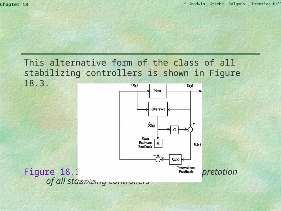
This alternative form of the class of all stabilizing controllers is shown in Figure 18.3.

Figure 18.3: State-estimate feedback interpretation of all stabilizing controllers


State-Space Interpretation of Internal Model Principle

A generalization of the above ideas on state-estimate feedback is the Internal Model Principle (IMP) described in Chapter 10. We next explore the state space form of IMP from two alternative perspectives.


(a) Disturbance-estimate feedback

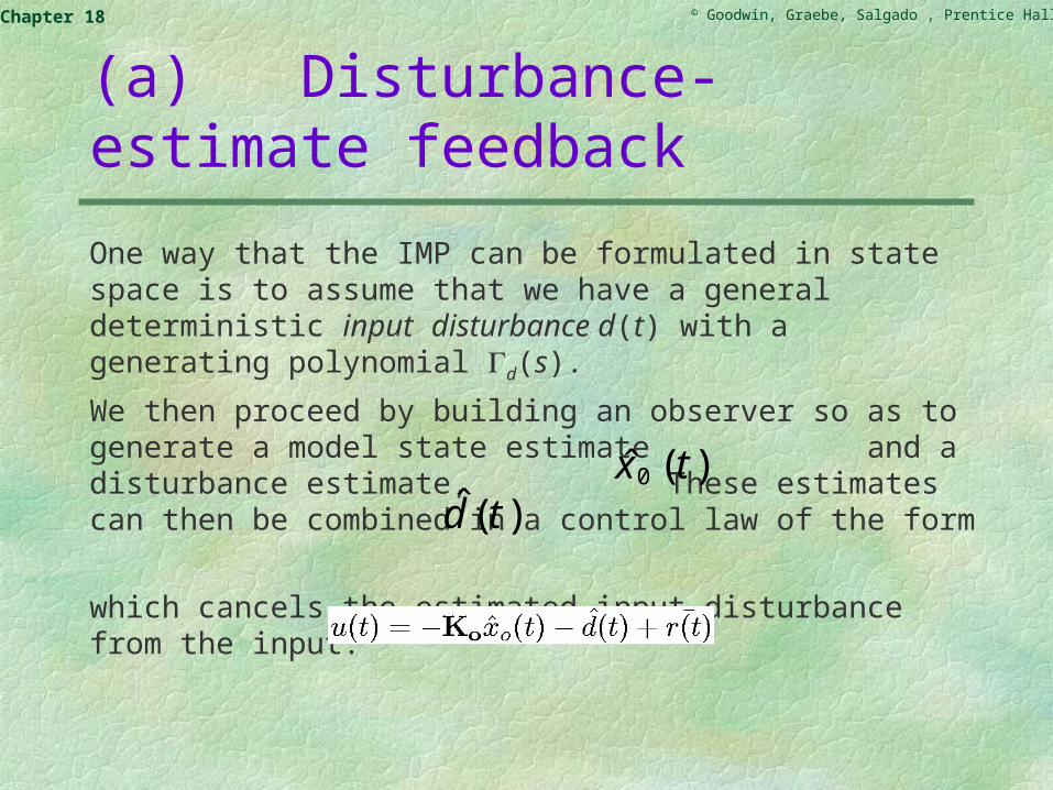
One way that the IMP can be formulated in state space is to assume that we have a general deterministic input disturbance d(t) with a generating polynomial d(s).

We then proceed by building an observer so as to generate a model state estimate and a disturbance estimate, These estimates can then be combined in a control law of the form

which cancels the estimated input disturbance from the input.

)(ˆ 0 tx).(ˆ td


We will show below that the above control law automatically ensures that the polynomial d(s) appears in the denominator, L(s), of the corresponding transfer-function form of the controller.


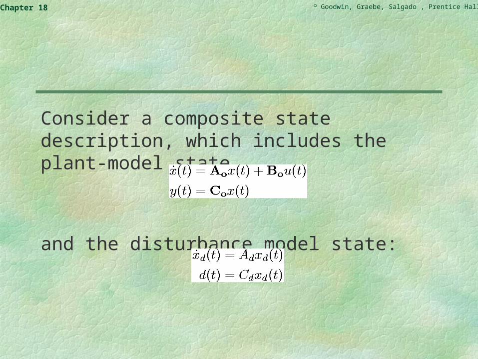
Consider a composite state description, which includes the plant-model state

and the disturbance model state:


We note that the corresponding 4-tuples that define the partial models are (A0, B0, C0, 0) and (Ad, 0, Cd, 0) for the plant and disturbance, respectively. For the combined state we have

The plant-model output is given by

,)()(0TT

dT txtx


Note that this composite model will, in general, be observable but not controllable (on account of the disturbance modes). Thus, we will only attempt to stabilize the plant modes, by choosing K0 so that (A0 - B0K0) is a stability matrix.

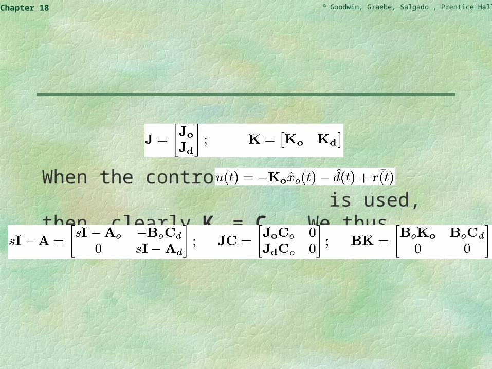
The observer and state-feedback gains can then be partitioned as on the next slide.


When the control law is used, then, clearly Kd = Cd. We thus obtain


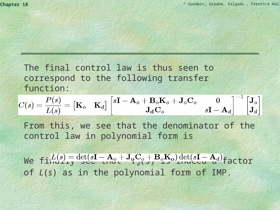
The final control law is thus seen to correspond to the following transfer function:

From this, we see that the denominator of the control law in polynomial form is

We finally see that d(s) is indeed a factor of L(s) as in the polynomial form of IMP.


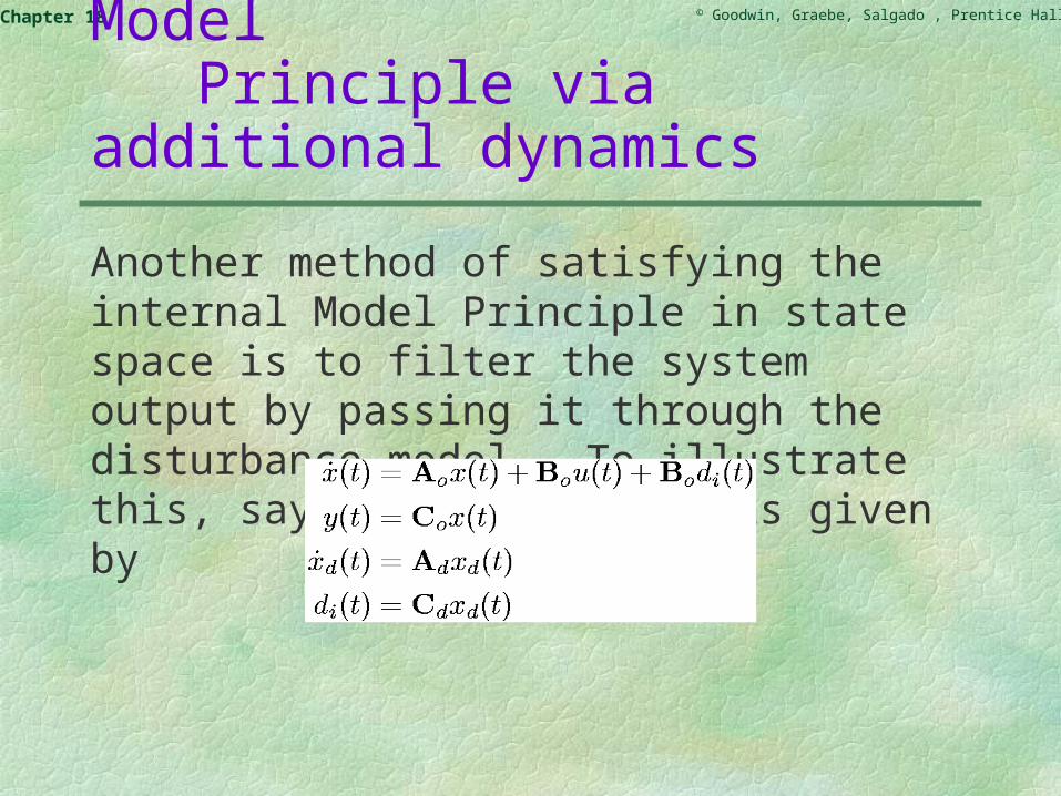
(b) Forcing the Internal ModelPrinciple via additional dynamics

Another method of satisfying the internal Model Principle in state space is to filter the system output by passing it through the disturbance model. To illustrate this, say that the system is given by


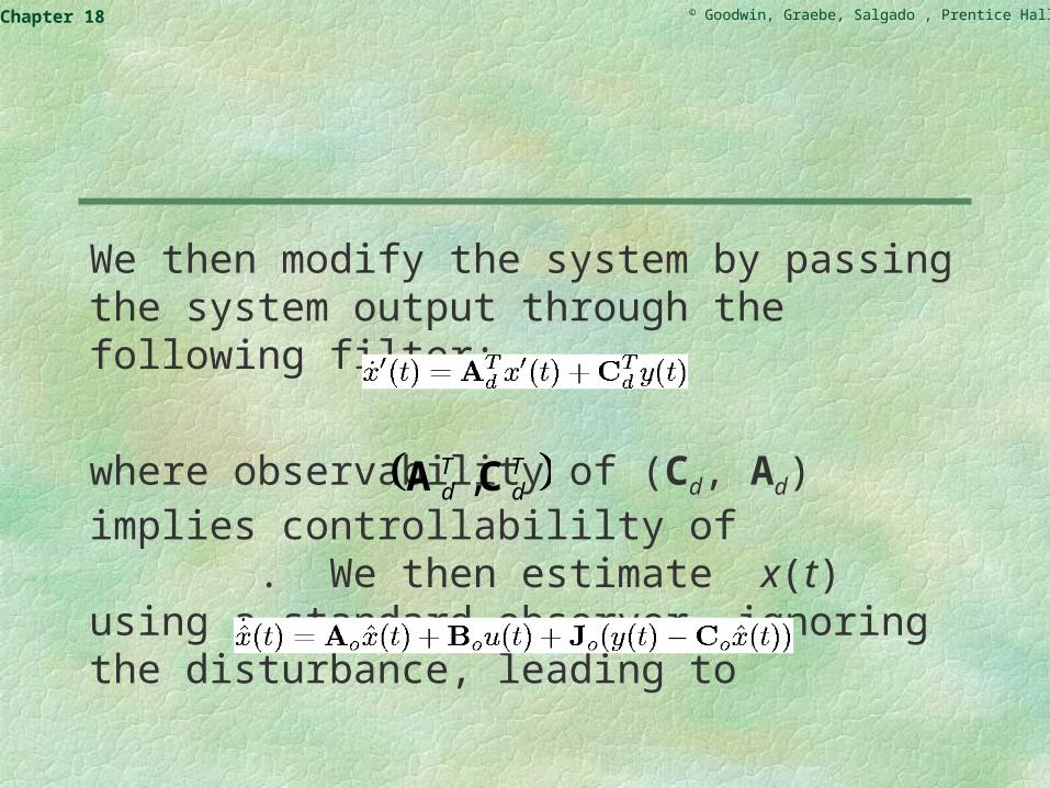
We then modify the system by passing the system output through the following filter:

where observability of (Cd, Ad) implies controllabililty of . We then estimate x(t) using a standard observer, ignoring the disturbance, leading to

Td

Td CA ,


The final control law is then obtained by feeding back both and to yield

where [K0, Kd] is chosen to stabilize the composite system.

)(ˆ tx )( tx


The results in section 17.9 establish that the cascaded system is completely controllable, provided that the original system does not have a zero coinciding with any eigenvalue of Ad.


The resulting control law is finally seen to have the following transfer function:

The denominator polynomial is thus seen to be

and we see again that d(s), is a factor of L(s) as required.


Dealing with Input Constraints in the Context of State-Estimate Feedback

We give a state space interpretation to the anti-wind-up schemes presented in Chapter 11.

We remind the reader of the two conditions placed on an anti-wind-up implementation of a controller,

(i) the states of the controller should be driven by the actual plant input;

(ii) the state should have a stable realization when driven by the actual plant input.


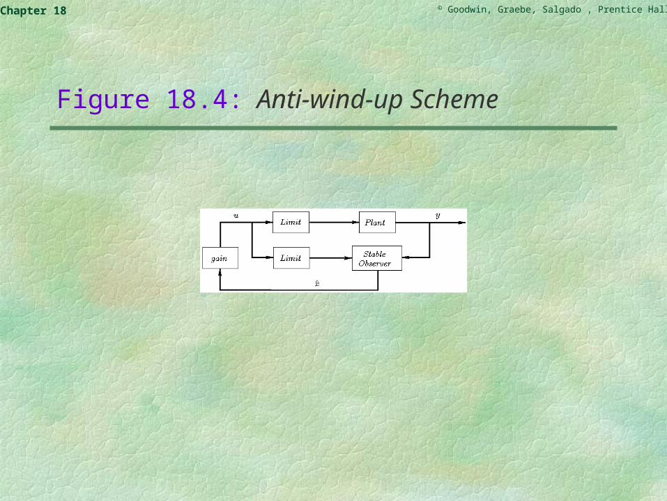
The above requirements are easily met in the context of state-variable feedback. This leads to the anti-wind-up scheme shown in Figure 18.4.


Figure 18.4: Anti-wind-up Scheme


In the above figure, the state should also include estimates of disturbances. Actually, to achieve a one-degree-of-freedom architecture for reference injection, then all one need do is subtract the reference prior to feeding the plant output into the observer.

We thus see that anti-wind-up has a particularly simple interpretation in state space.

x̂


Summary

We have shown that controller synthesis via pole placement can also be presented in state space form:

Given a model in state space form, and given desired locations of the closed-loop poles, it is possible to compute a set of constant gains, one gain for each state, such that feeding back the states through the gains results in a closed loop with poles in the prespecified locations.

Viewed as a theoretical result, this insight complements the equivalence of transfer function and state space models with an equivalence of achieving pole placement by synthesizing a controller either as transfer function via the Diophantine equation or as consntant-gain state-variable feedback.


Viewed from a practical point of view, implementing this controller would require sensing the value of each state. Due to physical, chemical, and economic constraints, however, one hardly ever has actual measurements of all system states available.

This raises the question of alternatives to actual measurements and introduces the notion of s-called observers, sometimes also called soft sensors, virtual sensors, filter, or calculated data.

The purpose of an observer is to infer the value of an unmeasured state from other states that are correlated with it and that are being measured.


Observers have a number of commonalities with control systems:

they are dynamical systems; they can be treated in either the frequency or the time domain; they can be analyzed, synthesized, and designed; they have performance properties, such as stability, transients, and

sensitivities; these properties are influenced by the pole-zero patterns of their

sensitivities.


State estimates produced by an observer are used for several purposes:

constraint monitoring; data logging and trending; condition and performance monitoring; fault detection; feedback control.

To implement a synthesized state-feedback controller as discussed above, one can use state-variable estimates from an observer in lieu of unavailable measurements; the emergent closed-loop behavior is due to the interaction between the dynamical properties of system, controller, and observer.


The interaction is quantified by the third-fundamental result presented in this chapter: the nominal poles of the overall closed loop are the union of the observer poles and the closed-loop poles induced by the feedback gains if all states could be measured. This result is also known as the separation theorem.

Recall that controller synthesis is concerned with how to compute a controller that will give the emergent closed loop a particular property, the constructed property.

The main focus of the chapter is on synthesizing controllers that place the closed-loop poles in chosen locations; this is a particular constructed property that allows certain design insights to be achieved.


There are, however, other useful constructed properties as well.

Examples of constructed properties for which there exist synthesis solutions:

to arrive at a specified system state in minimal time with an energy constraint;

to minimize the weighted square of the control error and energy consumption;

to achieve minimum variance control.


One approach to synthesis is to ease the constructed property into a so-called cost-functional, objective function or criterion, which is then minimized numerically.

This approach is sometimes called optimal control, because one optimizes a criterion.

One must remember, however, that the result cannot be better than the criterion.

Optimization shifts the primary engineering task from explicit controller design to criterion design, which then generates the controller automatically.

Both approaches have benefits, including personal preference and experience.

Documents

© Goodwin, Graebe, Salgado, Prentice Hall 2000 Chapter 18 Synthesis via State Space Methods