Embed Size (px)
Citation preview

! "!
"!Atmospheric composition, irreversible climate change, and mitigation policy #!
$!S. Solomon1,2, R. Pierrehumbert3, D. Matthews4, J. S. Daniel5 and P. Friedlingstein6 %!
&!1Department of Earth, Atmospheric, and Planetary Sciences, Massachusetts Institute of Technology, '!Cambridge, MA 02139 (!2Department of Atmospheric and Oceanic Sciences, University of Colorado, Boulder, CO 80309 )!3The University of Chicago, Department of the Geophysical Sciences, 5734 S. Ellis Ave, Chicago, IL *!60637 "+!4Department of Geography, Planning and Environment, Concordia University, Montreal, Quebec, Canada ""!H3G 1M8 "#!5Chemical Sciences Division, Earth System Research Laboratory, NOAA, Boulder, CO 80305 "$!6College of Engineering, Mathematics and Physical Sciences, University of Exeter, Exeter, EX4 4QF, UK "%! "&! "'!
Abstract "(!
The Earth’s atmosphere is changing due to anthropogenic increases of gases and aerosols ")!
that influence the planetary energy budget. Policy has long been challenged to ensure "*!
that instruments such as the Kyoto Protocol or carbon trading deal with the wide range of #+!
lifetimes of these radiative forcing agents. Recent research has sharpened scientific #"!
understanding of how climate system time scales interact with the time scales of the ##!
forcing agents themselves. This has led to an improved understanding of metrics used to #$!
compare different forcing agents, and has prompted consideration of new metrics such as #%!
cumulative carbon. Research has also clarified the understanding that short-lived #&!
forcing agents can “trim the peak” of coming climate change, while long-lived agents, #'!
especially carbon dioxide, will be responsible for at least a millennium of elevated #(!
temperatures and altered climate, even if emissions were to cease. We suggest that #)!
these vastly differing characteristics imply that a single basket for trading among forcing #*!
agents is incompatible with current scientific understanding. $+!
$"!
$#!
! #!
$$!
1. Introduction $%!
$&!
Anthropogenic increases in the concentrations of greenhouse gases and aerosols perturb $'!
the Earth’s energy budget, and cause a radiative forcing1 of the climate system. $(!
Collectively, greenhouse gases and aerosols can be considered radiative forcing agents, $)!
which lead to either increased (positive forcing) or decreased (negative forcing) global $*!
mean temperature, with associated changes in other aspects of climate such as %+!
precipitation and sea level rise. Here we briefly survey the range of anthropogenic %"!
greenhouse gases and aerosols that contribute to present and future climate change, %#!
focusing on time scales of the global anthropogenic climate changes and their %$!
implications for mitigation options. %%!
%&!
Differences in atmospheric residence times across the suite of anthropogenic forcing %'!
agents have long been recognized. As decision makers weigh near-term and long-term %(!
mitigation actions and tradeoffs, residence times of forcing agents are important along %)!
with social, economic, and political issues, such as climate change impacts, costs, and %*!
risks sustained by later versus earlier generations (and how these are valued). Recent &+!
research has rekindled and deepened the understanding (advanced by Hansen et al., 1997; &"!
Shine et al., 2005) that climate changes caused by anthropogenic increases in gases and &#!
aerosols can last considerably longer than the gases or aerosols themselves, due to the &$!
key role played by the time scales and processes that govern climate system responses. &%!
!!!!!!!!!!!!!!!!!!!!!!!!!!!!!!!!!!!!!!!!!!!!!!!!!!!!!!!!"!,-./-0/12!3456/78!/9!.23/72.!:2;8;<!=>??<!#++(@!-9!0A2!6A-782!/7!0A2!720!/55-./-762!:.4B7B-5.!C/7D9!DEB-5.<!82725-FFG!2HE52992.!/7!I!CJ#@!-0!0A2!054E4E-D92!.D2!04!-!6A-782!/7!-7!2H0257-F!.5/125!43!0A2!K-50AL9!27258G!MD.820<!9D6A!-9<!345!2H-CEF2<!-!6A-782!/7!0A2!64762705-0/47!43!6-5M47!./4H/.2;!!!!!

! $!
The climate changes due to the dominant anthropogenic forcing agent, carbon dioxide, &&!
should be thought of as essentially irreversible on time scales of at least a thousand years &'!
(Matthews and Caldeira, 2008; Plattner et al., 2008; Solomon et al., 2009, 2010). &(!
&)!
The largely irreversible nature of the climate changes due to anthropogenic carbon &*!
dioxide has stimulated a great deal of recent research, which is beginning to be '+!
considered within the policy community. Some research studies have focused on how '"!
cumulative carbon dioxide may represent a new metric of utility for policy, as a result of '#!
the identification of a near-linear relationship between its cumulative emissions and '$!
resulting global mean warming. In this paper, we discuss the use of cumulative carbon '%!
to help frame present and future climate changes and carbon policy formulation. We '&!
also briefly summarize several other metrics such as e.g., carbon dioxide equivalent ''!
concentration, the global warming potential (GWP) and global temperature change '(!
potential (GTP). Finally, we examine how current scientific understanding of the ')!
importance of time scales not just of different forcing agents, but also of their interactions '*!
with the climate system, sharpens the identification of approaches to formulate effective (+!
mitigation policies across a range of radiative forcing agents. ("!
(#!
2. The mix of gases and aerosols contributing to climate change ($!
(%!
A great deal of recent research has focused on understanding changes in atmospheric (&!
composition, chemistry, and the individual roles of the range of forcing agents and ('!
precursor emissions (leading to the formation of indirect forcing agents after emission) as ((!
! %!
contributors to observed and future climate change (Forster et al., 2007; Montzka et al., ()!
2011). It is not our goal to review that literature here, but rather to briefly summarize the (*!
state of knowledge of contributions of different species to global radiative forcing and )+!
time scales of related climate change, and to identify some implications for mitigation )"!
policy. )#!
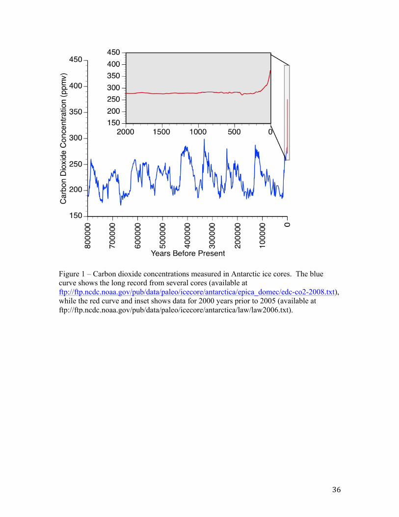
The concentrations of the major greenhouse gases carbon dioxide, methane, and nitrous )$!
oxide have increased due to human activities, and ice core data show that these gases )%!
have now reached concentrations not experienced on Earth in at least several thousand )&!
years (Luthi et al., 2008; Joos and Spahni, 2008; MacFarling-Meure et al., 2008). )'!
Figure 1 depicts the dramatic increase in carbon dioxide that has taken place over about )(!
the past century. The recent rates of increase in CO2, CH4, and N2O are unprecedented ))!
in at least 20,000 years (Joos and Spahni, 2008). The abundances of CO2, N2O and )*!
CH4 are well-mixed over the globe, and hence their concentration changes (and radiative *+!
forcings) are well characterized from data such as that shown in Figure 1; see Table 1. *"!
*#!
If anthropogenic emissions of the various gases were to cease, their concentrations would *$!
decline at a rate governed by physical and chemical processes that remove them from the *%!
global atmosphere. Most greenhouse gases are destroyed by photochemistry in the *&!
Earth’s atmosphere, including direct photolysis and attack by highly reactive chemical *'!
species such as the OH free radical. Many aerosols are removed largely by washout. *(!
Carbon dioxide is a unique greenhouse gas that is subject to a series of removal processes *)!
and biogeochemical cycling with the ocean and land biosphere, and even the lithosphere, **!
leading to a very long “tail” characterizing a portion of its removal (Archer et al., 1997). "++!

! &!
While the carbon dioxide concentration changes and anthropogenic radiative forcing "+"!
since 1750 are very well established, the relationship of its concentration changes to "+#!
changes in emission (including those from land use) is much less well characterized, due "+$!
to the flow of those emissions through the carbon cycle. A few industrial greenhouse "+%!
gases have lifetimes of many hundreds or even thousands of years, due to their extreme "+&!
chemical and photochemical stability and represent nearly “immortal” chemicals; in "+'!
particular, the fully fluorinated compounds such as CF4, NF3, and C2F6 fall in this "+(!
category. These gases also are strong absorbers of infrared radiation on a per molecule "+)!
basis. While these gases are currently present in very small concentrations, like carbon "+*!
dioxide their contributions to climate change are essentially irreversible on thousand year ""+!
time scales even if policies were to lead to reduced or zero emissions. """!
Table 1 summarizes the lifetimes (or, in the case of CO2, multiple removal time scales) ""#!
that influence the contributions of the range of gases and aerosols to radiative forcing and ""$!
climate change. Some related uncertainties in lifetimes and distributions are also ""%!
highlighted. ""&!
Direct emissions and other human actions (such as land disturbances, and emissions of ""'!
precursor gases) have increased the atmospheric burdens of particles, including mineral ""(!
dust, black carbon, sulfate, and organics. Tropospheric ozone has also increased largely "")!
as a result of emissions of precursor gases such as nitric oxide and organic molecules ""*!
including volatiles as well as methane. Indirect forcings linked to atmospheric aerosols "#+!
involving changes in clouds may also be very important, and are subject to very large "#"!
uncertainties (Forster et al., 2007). The short atmospheric lifetimes of aerosols and "##!
tropospheric ozone lead to very large variations in their abundances depending upon "#$!

! '!
proximity to local sources and transport, increasing the uncertainty in estimates of their "#%!
global mean forcing as well as its spatial distribution (see Table 1). "#&!
"#'!
Observations (e.g. of total optical depth by satellites or ground-based methods) constrain "#(!
the net total optical depth, or the transparency of the atmosphere, and provide information "#)!
on the total direct radiative forcing due to the sum of all aerosols better than they do the "#*!
forcing due to individual types of aerosol. Many aerosols are observed to be internal "$+!
mixtures, i.e., of mixed composition such as sulfate and organics, which substantially "$"!
affects optical properties and hence radiative forcing (see the review by Kanakidou et al., "$#!
2005, and references therein). Aerosols lead to perturbations of the top-of-atmosphere "$$!
and surface radiation budgets that are highly variable in space, and depend on the place as "$%!
well as amount of emissions. Limited historical data for emissions or concentrations of "$&!
aerosols imply far larger uncertainties in their radiative forcings since pre-industrial times "$'!
than for the well-mixed gases (see Table 1). Current research focuses on understanding "$(!
the extent to which some regional climate changes may reflect local climate feedbacks to "$)!
global forcing (e.g., Boer and Yu, 2003a,b), versus local responses to spatially variable "$*!
forcings. For example, increases in local black carbon and tropospheric ozone (e.g., "%+!
Shindell and Faluvegi, 2009) may have contributed to the high rates of warming observed "%"!
in the Arctic compared to other parts of the globe. Sulfate aerosols (which are present in "%#!
higher concentrations in the northern hemisphere due to industrial emissions) have been "%$!
suggested as a driver of changes in the north-south temperature gradients and rainfall "%%!
patterns (e.g., Rotstayn and Lohmann, 2002; Chang et al., 2011). Shortwave-absorbing "%&!
aerosols change the vertical distribution of solar absorption, causing energy that would "%'!

! (!
have been absorbed at the surface and communicated upward by convection to be directly "%(!
absorbed in the atmosphere instead; this can potentially lead to changes in precipitation "%)!
and atmospheric circulation even in the absence of warming (e.g. Menon et al. 2002). The "%*!
large uncertainties in the short-lived forcing terms as well as the regional climate signals "&+!
they may be inducing have heightened interest in their relevance for mitigation policy, "&"!
and this is discussed further below (see e.g., Ramanthan and Feng, 2008; Jackson, 2009; "&#!
Hansen et al., 1997; Jacobson, 2002; UNEP, 2011; Shindell et al., 2012). "&$!
"&%!
3. Metrics "&&!
Given the very broad diversity of anthropogenic substances with the potential to alter "&'!
Earth’s climate (e.g., CO2, CH4, N2O, SF6, CFCs, HFC’s, absorbing and reflecting "&(!
aerosols, chemical precursors, etc.), it is a challenging task to compare the climate effect "&)!
of a unit emission of (for example) carbon dioxide, with one of methane or sulfur "&*!
dioxide. Nevertheless, there has been a demand for such comparisons, and various "'+!
metrics have been proposed. The purpose of such metrics is to boil a complex set of "'"!
influences down to a few numbers that can be used to aid the process of thinking about "'#!
how different emissions choices would affect future climate. Among other uses, metrics "'$!
have been used to simplify the formulation of climate-related policy actions, climate-"'%!
protection treaties and emissions trading schemes. We suggest that to the extent "'&!
possible, a metric (or set of metrics) should not impose value judgments, least of all "''!
hidden value judgments (see Fuglestvedt et al., 2003). Metrics should provide a "'(!
simplified yet clear set of tools that the policy makers can use to formulate policy "')!
implementations to achieve an agreed set of climate protection ends. "'*!
! )!
"(+!
"("!
3.1 Radiative forcing and CO2-equivalent concentration "(#!
Radiative forcing is one measure of the influence of the burden of a range of forcing "($!
agents on the Earth’s radiative budget at a given point in time. A closely related metric "(%!
sometimes used to compare the relative effects of the range of forcing agents is to express "(&!
them as CO2-equivalent concentrations, which is the concentration of CO2 that would "('!
cause the same radiative forcing at the chosen time as a given mix of CO2 and other "((!
chemicals (including greenhouse gases and aerosols). "()!
"(*!
Figure 2 shows the CO2-equivalent concentration estimates for a range of major forcing ")+!
agents based on radiative forcing for 2005 from Forster et al. (2007), as given in NRC ")"!
(2011). The figure shows that among the major forcing agents, by far the largest ")#!
uncertainties stem from aerosols. Because aerosols represent a substantial negative ")$!
forcing (cooling effect), this leads to large uncertainty in the net total CO2-equivalent ")%!
concentration that is driving current observed global climate change. Current warming ")&!
represents a transient response that is about half as large as it would become in the long ")'!
term quasi-equilibrium state if radiative forcing were to be stabilized (NRC, 2011). ")(!
Therefore, uncertainties in today’s total CO2-equivalent concentration imply large "))!
uncertainties in how close current loadings of forcing agents may be to eventually ")*!
warming the climate by more than the 2°C target noted in the Copenhagen Accord. As "*+!
Figure 2 shows, uncertainties in aerosols dominate the uncertainties in total net radiative "*"!

! *!
forcing or total CO2-equivalent concentration. If aerosol forcing is large, then much of "*#!
the radiative effect of increases in greenhouse gases is currently being masked by "*$!
cooling, implying a larger climate sensitivity and far greater risk of large future climate "*%!
change than if aerosol forcing is small. "*&!
"*'!
A key limitation of radiative forcing or CO2-equivalent concentrations as metrics is that "*(!
they do not include any information about the time scale of the impact of the forcing "*)!
agent. For example, the radiative forcing for a very short-lived forcing agent may be "**!
very high at a given time but would drop rapidly if emissions were to decrease, while a #++!
longer-lived constituent implies a commitment to further climate change even if #+"!
emissions were to stop altogether. #+#!
#+$!
Insofar as short-lived aerosols produce a cooling, their masking of a part of the impact of #+%!
the large load of long-lived warming agents implies that an unseen long-term #+&!
commitment has already been made to more future warming (e.g. Armour and Roe, 2011; #+'!
Ramanathan and Feng, 2008); Hansen describes this as a “Faustian bargain”, since short-#+(!
lived aerosol masking can be accompanied by accumulation of more long-lasting and #+)!
hence ultimately more dangerous levels of carbon dioxide and other long-lived #+*!
greenhouse gases in the atmosphere (e.g., Hansen and Lacis, 1990). #"+!
#""!
It is evident that other metrics beyond radiative forcing are needed to capture temporal #"#!
aspects of the climate change problem. One needs to compare not only the effect of #"$!
various substances on today’s climate change but also how current and past emissions #"%!

! "+!
affect future climate change. As will be shown, available metrics all simplify or neglect #"&!
aspects of temporal information related to individual gases (albeit in different ways), and #"'!
hence incorporate choices and judgments rather than representing “pure” physical science #"(!
metrics (Fuglestvedt et al., 2003; Manne and Richels, 2001; O’Neill, 2000; Manning and #")!
Reisinger, 2011; Smith and Wigley, 2000; Shine, 2009). #"*!
##+!
The problem of formulating a metric for comparing climate impacts of emissions of ##"!
various greenhouse gases is challenging because it requires consideration of the widely ###!
differing atmospheric lifetimes of the gases. Emissions metrics are of most interest, ##$!
since it is emissions (rather than concentrations) that are subject to direct control. The ##%!
lifetime affects the way concentrations are related to emissions. For a short-lived gas like ##&!
CH4, the concentrations are a function of emissions averaged over a relatively short ##'!
period of time (on the order of a few decades in the case of CH4). For example, while ##(!
anthropogenic emissions increase, the CH4 concentration increases but if anthropogenic ##)!
emissions of CH4 were to be kept constant, the concentration of the gas would reach a ##*!
plateau within a few decades. In contrast, for a very persistent gas like CO2, the #$+!
concentration is linked to the cumulative anthropogenic emission since the time when #$"!
emissions first began; concentrations continue to increase without bound so long as #$#!
emissions are significantly different from zero. In essence, a fixed reduction of emission #$$!
rate of a short-lived gas yields a step-reduction in radiative forcing, whereas the same #$%!
reduction of emission rate of a very long-lived gas only yields a reduction in the rate of #$&!
growth of radiative forcing. #$'!
#$(!

! ""!
3.2 GWPh and GTPh #$)!
#$*!
The most familiar and widely applied metric for comparing greenhouse gases with #%+!
disparate atmospheric lifetimes is the Global Warming Potential (GWP). The GWP is #%"!
defined as the ratio of the time-integrated (over some time horizon) radiative forcing due #%#!
to a pulse emission of a unit of a given gas, to an emission of the same amount of a #%$!
reference gas (Forster et al., 2007). This can be expressed as: #%%!
#%&!
GWPh = !!!! !C(t) dt / !!!!!
! !Cr(t) dt (1) #%'!
#%(!
where h is a specified time horizon, !C(t) is the time series of the change in #%)!
concentration of the greenhouse gas under consideration (relative to some baseline #%*!
value), and !Cr(t) that of the reference gas (usually CO2. as we shall assume throughout #&+!
the following). !A (and !Ar) represent the radiative efficiencies due to changes in #&"!
concentration of the greenhouse gas (and reference gas) following a pulse emission at #&#!
t=0. In the remainder of this paper, we refer specifically to GWPh and GTPh to #&$!
emphasize the key role of the time horizon. If the pulse is small enough, the radiative #&%!
forcing is linear relative to the size of the emission pulse; the conventional assumption is #&&!
therefore that GWPh is independent of the size of the pulse. This assumption of linearity #&'!
can lead to substantial errors when the GWPh is extrapolated from an infinitesimal pulse #&(!
to very large emissions. Such errors can arise from nonlinearities in the radiative forcing #&)!
due to changes in concentration of the emitted gas or that of the reference gas CO2. #&*!
#'+!

! "#!
For gases with short atmospheric lifetimes (e.g. methane), the peak of concentration #'"!
that immediately follows a pulse in emission decays rapidly to zero, leading to a strong #'#!
dependence of GWPh on the timescale over which it is calculated (h in Equation 1). Table #'$!
2.14 in Forster et al. (2007) gives GWPh for a variety of gases, with h = 20, 100 and 500 #'%!
years. Methane for example, has a 100-year GWPh (GWP100) of 25, but a GWP500 of only #'&!
7.6. The choice of time horizon is crudely equivalent to the imposition of a discount rate, #''!
albeit a discount rate that varies with lifetime of the gas (Manne and Richels, 2001), and #'(!
thus represents a value judgment. A choice of small h implies that one should not care #')!
that CO2 saddles the future with an essentially permanent alteration of climate, whereas #'*!
the choice of a very large h says that one should not care about the transient warming due #(+!
to short-lived greenhouse gases. Either assumption embeds a judgment regarding whether #("!
the near term future is to be valued above the long term future, or vice versa. #(#!
#($!
An additional concern with the GWPh is that it represents only the change in integrated #(%!
forcing due to the emission of different gases, rather than the change in (for example) #(&!
global-mean temperature. This has led to the proposal of modified metrics, such as the #('!
Global Temperature Potential (GTPh) put forward by Shine et al. (2005). The GTPh #((!
represents the temperature change at some point h in time (rather than time-integrated #()!
radiative forcing) resulting from the unit emission of a greenhouse gas, relative to the #(*!
same emission of carbon dioxide. #)+!
#)"!
In order to illustrate some of the consequences of using GTPh or GWPh as climate change #)#!
metrics for gases of different atmospheric lifetimes, we use a simple two-layer ocean #)$!
! "$!
model to translate radiative forcing and surface temperature change over time. This #)%!
model is a simpler version of the upwelling-diffusion model used in Shine et al.(2005) to #)&!
critique GWPh, and has also been proved useful in analyzing the transient climate #)'!
response in full general circulation models (Winton et al, 2010; Held et al., 2010). The #)(!
model consists of a shallow mixed layer with temperature anomaly dT’mix and heat #))!
capacity μmix coupled to a deep ocean with temperature anomaly dT’deep and heat #)*!
capacity μdeep >> μmix. The mixed layer loses heat to space (in part via coupling to the #*+!
atmosphere) at a rate proportional to its temperature. The equations are #*"!
#*#!
mmix{dT'mix/dt } = -lT'mix - g(T'mix-T'deep) + !F(t) (2) #*$!
#*%!
mdeep{dT'deep/dt } = - g(T'deep-T'mix) (3) #*&!
#*'!
For constant radiative forcing !F, this model2 has the steady solution T’mix =T’deep = !F/l. #*(!
Hence 1/ l gives the quasi-equilibrium climate sensitivity. The model relaxes to this #*)!
equilibrium state on two time scales. On the short time scale (generally a matter of a few #**!
years), the mixed layer relaxes to a near-equilibrium with the atmosphere but the deep $++!
ocean has not yet had time to warm up, so T’deep " 0. The transient climate response $+"!
during this stage is then T’mix = !F/( l + g ). If !F is reduced to zero some time after the $+#!
deep ocean has warmed up to some nonzero value T’deep, then on the short mixed layer $+$!
time scale T’mix only falls to T’deep g/( l + g ), and subsequently relaxes to zero on the slow $+%!
deep ocean time scale. This term is the “recalcitrant warming” due to heat burial in the $+&!
!!!!!!!!!!!!!!!!!!!!!!!!!!!!!!!!!!!!!!!!!!!!!!!!!!!!!!!!#!The parameters we use in the following are: µdeep = 20µmix = 200J/m2K and ! = " = 2W/m2K.!

! "%!
deep ocean (Held et al., 2010). $+'!
$+(!
Figure 3(a) shows the calculated temperature response of the mixed layer in this model $+)!
due to pulse emissions of greenhouse gases with various lifetimes and forcing $+*!
efficiencies. In this calculation, the radiative forcing is assumed to be linear in the $"+!
concentration, and the concentration is assumed to decay exponentially with the stated $""!
lifetime. The magnitude of the emission of each gas is chosen so that all correspond to $"#!
the same value when weighted by GWP100; i.e., for a pulse emission, the radiative forcing $"$!
integrated over 100 years is identical in all cases. Figure 3 shows that the GWP100 $"%!
weighted emission for a gas with a 10-year (methane-like) lifetime and radiative $"&!
efficiency can be the same as for the longer lived gases, since a weaker long-term $"'!
warming can be compensated by a larger short term warming. If the integrated warming $"(!
over the 100 year period is all we care about, and the damages are linear in warming, then $")!
these cases may indeed all be considered to have identical impact in that the methane-like $"*!
case produces larger damages for a short time, as opposed to a longer period with smaller $#+!
damages for the longer-lived gases. However, if the objective is to limit the magnitude of $#"!
warming when the 100 year time span is reached, the use of GWP100 greatly exaggerates $##!
the importance of the short-lived gas, since virtually all of the warming has disappeared $#$!
after 100 years. This is a starting point for considering the value of the alternative concept $#%!
of Global Temperature-Change Potential (GTPh) as in Shine et al. (2005). Measured in $#&!
terms of 100-year GTPh, the 10-year lifetime gas has only 1/4.5 times the impact of e.g., $#'!
a 1000 year gas with identical GWP100. The warming after 100 years even in the 10-year $#(!
lifetime case has not decayed to zero as quickly as the radiative forcing itself (which has $#)!

! "&!
decayed by a factor of 4.5x10⁻⁵ over this time). The persistent, or recalcitrant warming $#*!
arises largely from ocean heat uptake (Solomon et al., 2010). But it should also be $$+!
emphasized that the 100-year GTPh does not capture the impact of the large short-term $$"!
warming from the methane-like case. Such short-term warming could be significant if, $$#!
for example, the near-term rate of temperature change were leading to adaptation stresses. $$$!
$$%!
Although GTPh may be a superior metric to GWPh for implementing climate protection $$&!
goals based on a threshold temperature at a given time, it does not resolve the problem of $$'!
sensitivity to the time frame chosen when computing the metric. Based on 100-year $$(!
GTPh, emitting an amount of a 1000-year lifetime gas might be considered to be about $$)!
twice as bad as an emission of a 50-year lifetime gas; however the long lived gas leads to $$*!
a warming that is nearly constant over the next 200 years whereas the warming due to the $%+!
50-year gas has largely disappeared by the end of that time. These two cases result in $%"!
radically different temperature changes over time and clearly do not represent identical $%#!
climate outcomes. $%$!
An additional problem with both GWPh and GTPh is their dependence on the emission $%%!
scenario. Figure 3a above represents the case of a pulse emission while Figure 3b shows $%&!
a second case with constant emissions of a methane-like gas with a 10-year lifetime, $%'!
compared to constant emissions of a gas with an infinite lifetime (see e.g., Shine, 2005). $%(!
In both Figures 3a and b, the emissions scenarios were selected such that the GWP100 $%)!
values are equivalent. Emissions are sustained for 200 years, and then set to zero at the $%*!
year 200. In both cases, the warming continues beyond the point at which the $&+!
concentration of the gas stabilizes; in the case of the methane-like gas, the concentration $&"!

! "'!
(not shown) stabilizes after about 10 years but warming continues to increase, illustrating $&#!
the continuing warming that occurs despite constant atmospheric concentrations, as the $&$!
deep ocean takes up heat. For the infinitely long-lived gas, concentrations remain $&%!
elevated even after emission stops, and warming continues to increase (see next section). $&&!
Indeed, although both cases are equivalent in terms of GWP100-weighted emissions, the $&'!
infinite-lifetime case leads to a warming that is not only larger at the end of 200 years, $&(!
but persists for centuries afterwards. The constant-emissions case illustrates the $&)!
dependence of GTPh on the emissions scenario. Neither GWPh nor GTPh capture what $&*!
occurs after emissions cease. $'+!
As a final example, we have carried out a series of calculations driven by the CO2 time $'"!
series computed in Eby et al. (2009). The concentration time series were computed by $'#!
driving an intermediate-complexity climate-carbon cycle model with historical emissions $'$!
up to the calendar year 2000, followed by two test scenarios in which the emissions rate $'%!
rises to a peak after 150 years, and then declines to zero in the subsequent 150 years. The $'&!
two scenarios shown in Figure 3c show results corresponding to 640GtC and 1280GtC of $''!
post-2000 cumulative carbon emissions (see next section). Note that the warming is $'(!
fairly constant in the 700 years following cessation of emission, given the realistic $')!
atmosphere CO2 used in this case as compared to the infinite-lifetime case shown in $'*!
Figure 3b. Abating cumulative carbon by 640GtC (the difference between the two $(+!
emission scenarios shown here) reduces warming by about 0.6K in the two-box model. $("!
$(#!
The dashed curves in Figure 3c show what happens if the radiative forcing from CO2 is $($!
augmented by that from methane released at a constant rate between 2000 and 2300, with $(%!

! "(!
the total emissions again equivalent to the CO2 from 640GtC based on weighting with a $(&!
GWP100 of 25 (Forster et al.(2007). The corresponding methane emission rate is 0.31 Gt $('!
per year, which is similar to the current anthropogenic emission rate of about 0.35 Gt per $((!
year (see http://cdiac.ornl.gov/trends/meth/ch4.htm). Emissions are stopped entirely in $()!
2300 in this example. One can think of the curve for 640GtC plus methane (dashed blue $(*!
line) as the result of deciding to abate CO2 emissions first and methane later, while the $)+!
curve with 1280GtC and no methane (solid black line) corresponds to abating methane $)"!
first and carbon later. It is useful to compare the “Methane First” to that for the “CO2 $)#!
First” case, recalling that both have the same GWP100 weighted emissions. The blue $)$!
dashed curve ramps up quickly and faster just after 2000 as expected from having more $)%!
short-lived CH4. Overall, the two track quite well for the first 100 years (compare the $)&!
solid black line with the dashed blue line), but thereafter the temperature for “CO2 First” $)'!
falls well below that for “Methane First.” Moreover, after methane emissions are $)(!
eliminated, the dashed blue line (“CO2 First”) case converges with the curve for 640GtC $))!
alone (solid blue line) within a century, as if methane had never been emitted at all. $)*!
Figure 3c highlights the comparison between the two curves representing the “Methane $*+!
First” vs. “CO2 First” strategies. The shaded region mirrors the analysis of (Daniel et al $*"!
2011), who used emissions and climate response models that were less idealized. The $*#!
general lesson to be learned is that over the universe of strategies considered equivalent $*$!
with regard to GWP100, an emphasis on short-lived forcing agents yields more near-term $*%!
moderation of warming but comes at the expense of considerably greater long term $*&!
warming. $*'!
$*(!

! ")!
A comparison of the bottom two curves in Figure 3c, in contrast, illustrates the “peak $*)!
trimming” benefits of reductions in short-lived forcing agents. However, a comparison of $**!
the lower two curves alone gives an incomplete picture of the decision framework. One %++!
will always get more warming reduction from doing two beneficial things rather than one %+"!
beneficial thing, but the real question is whether one would get a still better consequence %+#!
by putting added resources into further reductions of CO2 versus applying them to short-%+$!
lived agents. %+%!
%+&!From the examples in Figure 3, it is clear that emissions of methane (and similarly other %+'!
short-lived radiative forcing agents) have a strong bearing on the amount of warming %+(!
during the time over which they are emitted, but have little lasting consequence for the %+)!
climate system. By contrast, CO2 and (and to a lesser extent other long-lived forcing %+*!
agents) are relevant to both short- and long-term climate warming, and in particular %"+!
generate warming which persists at significant levels long after emissions are eliminated. %""!
These fundamental differences between short- and long-lived radiative forcing agents %"#!
cannot be captured by either GWPh or GTPh metrics, which by design can only provide %"$!
comparisons for the chosen time horizon. Here we have illustrated key limitations of %"%!
such an approach over time. %"&!
%"'!
3.3. Irreversibility of CO2-induced warming, climate commitment, and the cumulative %"(!
CO2 emissions metric %")!
As illustrated above, whereas shorter-lived gases and aerosols have a strong bearing on %"*!
near-future climate changes, warming that persists beyond the 21st century, and %#+!
particularly warming that persists beyond the period of time that humans emit %#"!

! "*!
greenhouses gases, will be primarily determined by how much carbon dioxide is emitted %##!
over this period of time. Because of the long lifetime of carbon dioxide in the %#$!
atmosphere compared to other major greenhouse gases, the long-term warming legacy of %#%!
anthropogenic greenhouse gases will be primarily determined by CO2-induced warming. %#&!
In recent literature, the concept of the irreversibility of climate change due to CO2 %#'!
emissions was first highlighted by Matthews and Caldeira (2008) based upon results from %#(!
an Earth Model of Intermediate Complexity (EMIC). This has led to the recognition that %#)!
cumulative carbon (the total tonnes of carbon emitted) has particular utility for policy. %#*!
Matthews and Caldeira (2008) showed that if CO2 emissions were eliminated, globally-%$+!
averaged temperature stabilized and remained approximately constant for several %$"!
hundred years; notably, though CO2 concentrations decreased in the atmosphere, %$#!
temperatures remained at a nearly constant level, mainly as a result of a declining rate of %$$!
heat uptake by the ocean that approximately balances the decline in carbon dioxide %$%!
levels; for a detailed discussion see Solomon et al. (2010). Several other EMIC studies %$&!
have also demonstrated the irreversibility of CO2-induced warming. Solomon et al %$'!
(2009) showed that even after 1000 years of model simulation following the elimination %$(!
of CO2 emissions, global temperatures were essentially irreversible, remaining within %$)!
about half a degree of their peak values for a broad range of emission rates and maximum %$*!
concentrations. In an intercomparison of eight EMICs, Plattner et al (2008) showed %%+!
persistence of high global temperatures for at least several centuries following zero %%"!
emissions across all the models. More comprehensive global climate models require %%#!
much more computer time and hence have thus far been run for zero emission tests over %%$!
multiple centuries rather than millennia, and show similar results (Lowe et al 2009 and %%%!

! #+!
Gillett et al 2011). These studies have confirmed that irreversibility of CO2-induced %%&!
warming is a property of the climate system that is driven by basic properties of the %%'!
system, notably the carbon and ocean heat timescales, and is not limited to intermediate-%%(!
complexity models. %%)!
This body of literature has all contributed to estimating what has been called the “zero-%%*!
emissions commitment”; that is the anticipated future warming that occurs in the absence %&+!
of additional future CO2 emissions. This quantity is distinct from another widely-used %&"!
definition of committed warming: the “constant-composition commitment,” which is %&#!
defined as the future global temperature change which would be expected under constant %&$!
concentrations of atmospheric CO2 (Meehl et al., 2007). %&%!
The difference between these two measures of committed future warming was %&&!
highlighted by Matthews and Weaver (2011), and summarized in Figure 4a. Under %&'!
constant atmospheric CO2 concentrations, temperatures continue to increase as the %&(!
climate system slowly adjusts to the current atmospheric forcing from CO2 in the %&)!
atmosphere. By contrast, if CO2 emissions were set to zero, atmospheric CO2 would %&*!
decrease over time due to removal by carbon sinks, but global temperature would remain %'+!
approximately constant for several centuries. This difference can also be seen in the %'"!
example of the simple model shown above: constant composition of an infinite-lifetime %'#!
gas after year 200 in Figure 3b leads to increasing global temperatures, whereas zero %'$!
emissions of CO2 at the year 2300 in Figure 3c leads to approximately stable global %'%!
temperatures. Persistent warming over many centuries is especially relevant for %'&!
understanding impacts including the large sea level rise that occurs in a warmer world %''!
due to slow thermal expansion of the deeper parts of the ocean and the potentially very %'(!

! #"!
gradual loss of the great ice sheets of Greenland and Antarctica (Meehl et al., 2007 and %')!
references therein). %'*!
%(+!
The difference between the constant-composition and zero-emission commitment can %("!
also be understood in terms of the CO2 emissions associated with each scenario. Figure %(#!
4b shows the historical emissions in blue associated with both scenarios, and the future %($!
emissions in red required to maintain constant CO2 concentrations at year-2010 levels. %(%!
Given the required balance between emissions and removal by carbon sinks to maintain %(&!
constant atmospheric levels, the future emissions associated with a constant-composition %('!
scenario are substantially larger than zero; in this example, the total emissions over 300 %((!
years required to maintain constant atmospheric CO2 amount to about 250 GtC, or close %()!
to half of the total historical CO2 emissions (about 500 GtC). These future emissions are %(*!
consistent with the continued future warming associated with constant atmospheric CO2 %)+!
concentrations. By contrast, zero future emissions is consistent with near-zero additional %)"!
future warming. %)#!
As already noted, the removal of anthropogenic CO2 from the atmosphere involves a %)$!
multitude of time scales, ranging from a few decades for uptake by the upper ocean and %)%!
land biosphere, a millennium for uptake by the deep ocean, tens of millennia for %)&!
carbonate dissolution and weathering to restore ocean alkalinity and allow further uptake, %)'!
and hundreds of thousands of years for silicate weathering (Archer et al, 1997). The %)(!
nonlinearity of the carbonate chemistry is important in determining the way climate %))!
change relates to larger and larger increases in CO2. Though the radiative forcing is %)*!

! ##!
logarithmic as a function of CO2 concentration, the carbonate chemistry implies that the %*+!
fraction of CO2 that remains in the atmosphere after emission increases with the %*"!
magnitude of the emission (Eby et al., 2009). Further, the slow decay in radiative forcing %*#!
due to ocean uptake of carbon following cessation of emissions occurs at roughly the %*$!
same time scale as the relaxation of the deep ocean temperature towards equilibrium; %*%!
because these two terms work in opposing directions, the surface temperature attained at %*&!
the time emissions cease is not only proportional to the cumulative carbon, but is also the %*'!
temperature which prevails with little change for roughly the next millennium (Matthews %*(!
and Caldeira, 2008; Solomon et al., 2009; Eby et al., 2009, Solomon et al. 2010). %*)!
%**!
The coherence between cumulative emissions of carbon dioxide and global temperature &++!
changes has been the subject of several recent studies, and represents a new metric with &+"!
which to assess the climate response to human CO2 emissions. Matthews et al (2009) and &+#!
Allen et al (2009) both identified a strong linear relationship between global temperature &+$!
change and cumulative carbon emissions. Matthews et al (2009) named this the “carbon-&+%!
climate response.”. In this study, they showed the carbon-climate response is well &+&!
constrained by both coupled climate-carbon models and historical observations to lie &+'!
between 1 and 2.1 °C per 1000 GtC emitted (see Figure 5 below, taken from NRC, 2011). &+(!
Allen et al (2009) used a simpler climate model, but considered a larger range of possible &+)!
climate sensitivities; as a result, they estimated that the instantaneous temperature change &+*!
associated with cumulative carbon emissions fell between 1.4 and 2.5 °C per 1000 GtC &"+!
emitted. &""!
! #$!
Cumulative carbon emissions provides a clear means of estimating the extent of climate &"#!
warming that will occur from wide range of future CO2 emissions scenarios. &"$!
Consequently, the anthropogenic warming that will occur, and which will persist for &"%!
many subsequent centuries, will be determined to a large extent by the total cumulative &"&!
emissions which occur between now and the time by which humans stop emitting &"'!
significant amounts of carbon dioxide. If a tipping point (Lenton et al., 2008) in the &"(!
earth system were to be experienced at any time in the future, even the immediate &")!
cessation of CO2 emissions will be unable to substantially lower the global temperature &"*!
even on timescales of tens of generations. &#+!
&#"!
4. Policy Outlook &##!
&#$!
Reducing emissions of shorter-lived gases and aerosols (e.g., black carbon) is indeed a &#%!
highly effective way to reduce climate forcing or the rate of warming on shorter &#&!
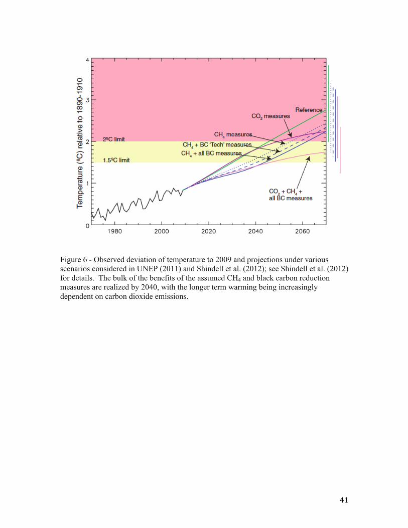
timescales as shown by many authors (see e.g. UNEP, 2011; Jacobson, 2002; Shindell et &#'!
al., 2012 and references therein), and illustrated here in Figure 6. But Figure 3 above &#(!
provides key context to better understand choices among policy options. In particular, &#)!
Figure 3c goes beyond the timescale shown in Figure 6 to illustrate that reductions of &#*!
short-lived gases or aerosols should be most appropriately thought of as an approach to &$+!
“trimming the peak” warming (and perhaps the rate of warming) in the near term (but &$"!
recall the discussion in connection with Figure 3, bearing on the question of choices &$#!
between efforts put into peak trimming versus additional CO2 reductions). Furthermore, &$$!
delays in the abatement of short lived forcing agents imply greater heat storage in the &$%!

! #%!
deep ocean and greater sea level rise; thus, the utility of the peak trimming is affected by &$&!
when it is implemented as well as by how much. Peak trimming can also reduce the rate &$'!
of warming, with attendant benefits for the ability of human and natural systems to adapt. &$(!
Greater benefits in peak trimming are obtained the sooner the emissions are abated (see &$)!
Held et al., 2010). However, Figure 3c also shows that the long term climate – i.e. the &$*!
character of the “Anthropocene” – is determined largely by the cumulative carbon &%+!
emitted. It is noteworthy that the use of GWP100 in a policy vehicle would consider the &%"!
”Methane First” scenario to be equivalent to the ”CO2 First” scenario, but the figure &%#!
makes clear that the latter yields a far better outcome if one is concerned about the &%$!
climate changes that last beyond 100 years. Thus Figure 3c demonstrates why trimming &%%!
the peak cannot substitute for reductions in carbon dioxide emissions that will dominate &%&!
Earth’s climate for many centuries if unabated. &%'!
&%(!
A key policy issue involves the relative reductions to make in the emissions of the range &%)!
of greenhouse gases. The Kyoto Protocol addressed this issue by placing the regulated &%*!
greenhouse gases into a single basket and relating their emissions in a common CO2-&&+!
equivalent emission determined by multiplying actual emissions with the 100-yr GWPh. &&"!
Numerous studies have demonstrated that using a single metric in this way has &&#!
drawbacks arising from the disparity in global lifetimes of the various gases. As we have &&$!
illustrated here, the choice of a particular time horizon includes value judgments &&%!
regarding the importance of climate changes at varying times. For example, if a GWPh &&&!
with a short time horizon is used in order to better equate short-term climate impacts &&'!
among gases, the larger relative impact of gases with long lifetimes over long timescales &&(!

! #&!
will not be considered. Perhaps more importantly, the use of the GWPh as the trading &&)!
metric leads to greenhouse gas trading based on relative integrated radiative forcing, &&*!
which has a limited connection to temperature change (as shown by the comparison of &'+!
GTPh to GWPh) but probably better represents sea level rise (Smith and Wigley, 2000). &'"!
Many studies have examined ways to more effectively address near-term and long-term &'#!
warming (e.g., Manne and Richels, 2001 and others), but the majority of policy &'$!
discussions have revolved around greenhouse gas metrics for a given time that cannot &'%!
account for time-varying policy goals. &'&!
&''!
The Montreal Protocol regulated ozone-depleting substances (ODSs) that were also &'(!
characterized by very different lifetimes. This Protocol was highly successful in reducing &')!
ozone depletion and took a different approach from that of the Kyoto Protocol. Rather &'*!
than group all ODSs into a single basket in which production and consumption reductions &(+!
could be traded using some metric like the ozone depletion potential (ODP), the Montreal &("!
Protocol effectively regulated groups of gases (e.g., CFCs, HCFC, halons) and some &(#!
individual gases (e.g., CH3CCl3, CCl4, CH3Br) separately. Members of these groups were &($!
largely characterized by similar lifetimes. It has been shown that if the Montreal Protocol &(%!
took an alternative single basket approach, and if trading among ODSs were possible and &(&!
were performed, the success of the Protocol in limiting short term risks could have been &('!
compromised (Daniel et al., 2011). &((!
&()!
The principal conclusion of the discussion presented in this paper is that the scientific &(*!
basis for trading among all greenhouse gases in one single basket is poor, and a more &)+!

! #'!
science-based approach for the Kyoto Protocol (and similar regulatory frameworks) &)"!
would be to abandon the idea of a single-basket approach altogether. As we have shown, &)#!
short-lived greenhouse gases or aerosols, and CO2 are knobs that control quite different &)$!
aspects of the future climate. It does not appear likely that any single metric will be able &)%!
to fairly represent both. Yet both time scales are clearly important from the policy &)&!
viewpoint of risks of different types of future climate changes, such as a possibly slow &)'!
loss of ice from Greenland and Antarctica over millennia and associated massive sea &)(!
level rise, versus the potential for rapid increases in the area burned by wildfire in the &))!
next decade or two. Thus, the research of the past few years shows even more clearly &)*!
than previous studies that the existing single-basket GWPh framework is difficult to &*+!
justify. &*"!
&*#!
Many of the problems with GWPh and GTPh are not intrinsic to the metrics themselves, &*$!
but to the imposition of a single time scale when computing the metric. As a minimum, a &*%!
two-basket approach seems to be needed. One basket could be CO2, and the metric used &*&!
to quantify the climate impact of that basket would be cumulative carbon emission &*'!
(Matthews et al., 2009). Further work is needed to determine whether perfluorocarbons &*(!
might also be included in this basket through a suitable adjustment of cumulative carbon. &*)!
The long-term basket should be recognized as the only path to managing long-term risks &**!
to the climate. The second basket would include much shorter-lived forcing agents such '++!
as CH4, tropospheric ozone, and black carbon, which could be grouped together and '+"!
measured by a metric such as the GTPh. Carbon dioxide can be considered here as well, '+#!
since its growth is expected to be important for the rate of climate change in the near term '+$!
! #(!
(as well as being not only dominant but controlling the changes in the long-term). '+%!
Reducing short-lived gases or aerosols does nothing to reduce the long-term risk posed '+&!
by substances such as carbon dioxide. This second basket would explicitly recognize '+'!
and manage what can be done to reduce warming in the short-term time scale of decades '+(!
or so, with the choice of time horizon h being essential. Such an approach would make '+)!
explicit that reducing short-lived forcing agents can “trim the peak” of global warming '+*!
but does not, as is sometimes erroneously stated, “buy time” to deal with carbon and '"+!
other gases (Biello, 2012), unless one neglects entirely the longer term impacts of current '""!
actions. A two-basket framework would require careful and interactive analysis of the '"#!
science, risks, and value judgments associated with choosing how much and when to '"$!
reduce the short-lived and long-lived baskets, and we believe that it would result in a '"%!
clearer path forward for mitigation policy. '"&!
'"'!
'"(!
References '")!
Allen, M. R., D. J. Frame, C. Huntingford, C. D. Jones, J. A. Lowe, M. Meinshausen, and '"*!
N. Meinshausen, Warming caused by cumulative carbon emissions towards the '#+!
trillionth tonne, Nature, 458 (7242), 1163–1166, doi:10.1038/nature08019, 2009. '#"!
Archer, D., H. Kheshgi, and E. Maier-Reimer, Multiple timescales for neutralization of '##!
fossil fuel CO2. Geophysical Research Letters 24 (4):405-408, 1997. '#$!
'#%!
Armour, K. C., and G. H. Roe, Climate commitment in an uncertain world, Geophys. '#&!
Res. Lett., 38, L01707, doi:10.1029/2010GL045850, 2011 '#'!

! #)!
Biello, D., (2012). http://www.scientificamerican.com/article.cfm?id=how-to-buy-time-'#(!
to-combat-climate-change-cut-soot-methane. '#)!
Boer, G.J., and B. Yu, Climate sensitivity and climate state, Clim. Dyn., 21, 167–176, '#*!
2003a. '$+!
'$"!
Boer, G.J., and B. Yu, Climate sensitivity and response, Clim. Dyn., 20, 415–429, 2003b. '$#!
'$$!
Caldeira K., and J. F. Kasting, Insensitivity Of global warming potentials to carbon '$%!
dioxide emission scenarios, Nature, 366, 251-253. doi:10.1038/366251a0, 1993. '$&!
'$'!
Chang, C.-Y., J. C. H. Chiang, M. F. Wehner, A. R. Friedman, and R. Ruedy, Sulfate '$(!
aerosol control of tropical Atlantic climate over the twentieth century, J. Climate, '$)!
24, 2540–2555. doi: 10.1175/2010JCLI4065.1, 2011. '$*!
'%+!
Daniel J. S., S. Solomon, T. J. Sanford, M. McFarland, J. S. Fuglestvedt and P. '%"!
Friedlingstein, Limitations of single-basket trading: lessons from the '%#!
Montreal Protocol for climate policy, Climatic Change, DOI: 10.1007/s10584-'%$!
011-0136-3, 2011. '%%!
'%&!
Eby, M., K. Zickfeld, A. Montenegro, D. Archer, K. J. Meissner, and A. J. Weaver, '%'!
Lifetime of anthropogenic climate change: millennial time scales of potential CO2 '%(!
and surface temperature perturbations, Journal of Climate 22 (10):2501-2511, '%)!
DOI: 10.1175/2008JCLI2554.1, 2009. '%*!

! #*!
'&+!
Forster, P., et al., Changes in atmospheric constituents and in radiative forcing, in '&"!
Climate Change 2007: The Physical Science Basis, (S. Solomon et al., eds.), pp. '&#!
129–234, Camb. Univ. Press, 2007. '&$!
'&%!
Fuglestvedt J. S., T. K. Berntsen, O. Godal, R. Sausen, K. P. Shine and T. Skodvin, '&&!
Metrics of climate change: assessing radiative forcing and emission indices. Clim '&'!
Change 58(3):267–331, 2003. '&(!
'&)!
Gillett, N. P., V. J. Arora, K. Zickfeld, S. J. Marshall, and W. J. Merryfield, Ongoing '&*!
climate change following a complete cessation of carbon dioxide emissions, ''+!
Nature Geoscience, 4, 83-87, 2011. ''"!
Hansen, J.E., and A.A. Lacis, Sun and dust versus greenhouse gases: An assessment of ''#!
their relative roles in global climate change. Nature, 346, 713-719, ''$!
doi:10.1038/346713a0, 1990. ''%!
Hansen, J., M. Sato, and R. Ruedy,Radiative forcing and climate response. J. Geophys. ''&!
Res. Atmos. 102, 6831–6864. (doi:10.1029/96JD03436), 1997. '''!
''(!
Hansen J et al., Efficacy of climate forcings, J. Geophys. Res., 110, D18104, '')!
doi:10.1029/2005JD005776, 2005. ''*!
'(+!
Held, I. M., M. Winton, K. Takahashi, T. Delworth, F. Zeng, and G. K. Vallis, Probing '("!

! $+!
the Fast and Slow Components of Global Warming by Returning Abruptly to '(#!
Preindustrial Forcing. J. Climate, 23, 24182427. doi: 10.1175/2009JCLI3466.1, '($!
2010. '(%!
'(&!
Jackson S. C., Parallel pursuit of near-term and long-term climate mitigation. Science '('!
326:526–527, 2009. '((!
Jacobson, M. Z., Control of fossil-fuel particulate black carbon and organic matter; '()!
possibly the most effective method of slowing global warming. J. Geophys. Res. '(*!
107, 4410–4431. (doi:10.1029/2001JD001376), 2002. ')+!
')"!
Joos, F., and R. Spahni, Rates of change in natural and anthropogenic radiative forcing ')#!
over the past 20000 years, Proc. Nat. Acad. Sci., 105, 1425-1430, doi: ')$!
10.1073/pnas.0707386105, 2008. ')%!
Kanakidou, M., J.H. Seinfeld, S.N. Pandis, I. Barnes, F.J. Dentener, M.C. Facchini, R. ')&!
Van Dingenen, B. Ervens, A. Nenes, C.J. Nielsen, E. Swietlicki, J.P. Putaud, Y. ')'!
Balkanski, S. Fuzzi, J. Horth, G.K. Moortgat, R. Winterhalter, C.E.L. Myhre, K. ')(!
Tsigaridis, E. Vignati, E.G. Stephanou, and J. Wilson, Organic aerosol and global '))!
climate modelling: A review, Atmos. Chem. Phys, 5, 1053-1123, ')*!
doi:10.5194/acp-5-1053-2005, 2005. '*+!
Lenton, T. M., H. Held, E. Kriegler, J. W. Hall, W. Lucht, S. Rahmstorf and H. J. '*"!
Schellnhuber, Tipping elements in the Earth’s climate system. Proc. Nat. Acad. '*#!
Sci., 105 (6) 1787-1793, 2008. '*$!

! $"!
Lowe, J. A., C. Huntingford, S. C. B. Raper, C. D. Jones, S. K. Liddicoat, and L. K. '*%!
Gohar, How difficult is it to recover from dangerous levels of global warming?, '*&!
Env. Res. Lett., 4, 014,012, 2009. '*'!
Luthi, D., et al. 2008 High-resolution carbon dioxide concentration record 650,000–'*(!
800,000 years before present, Nature 453, 379-382, doi:10.1038/nature06949, '*)!
2008. '**!
MacFarling-Meure, C., D. Etheridge, C. Trudinger, P. Steele, R. Langenfelds, T. van (++!
Ommen, A. Smith, and J. Elkins, Law Dome CO2, CH4 and N2O ice core records (+"!
extended to 2000 years BP, Geophysical Research Letters 33, L14810, 2006. (+#!
Manne, A. S., and R. G. Richels, An alternative approach to establishing trade-offs (+$!
among greenhouse gases. Nature 410, 675–677. (doi:10.1038/35070541), 2001. (+%!
(+&!
Manning, M. and A. Reisinger, Broader perspectives for comparing different greenhouse (+'!
gases, Phil. Trans. R. Soc. A 369, 1891–1905, doi:10.1098/rsta.2010.0349, 2011. (+(!
(+)!
Matthews, H. D., and K. Caldeira, Stabilizing climate requires near-zero emissions, (+*!
Geophys. Res. Lett., 35, L04,705, 2008. ("+!
(""!
Matthews, H. D., N. Gillett, P. A. Stott, and K. Zickfeld, The proportionality of global ("#!
warming to cumulative carbon emissions, Nature, 459, 829–832, 2009. ("$!
! $#!
Matthews, H. D. and A. J. Weaver, Committed climate warming, Nature Geoscience 3, ("%!
142 – 143, doi:10.1038/ngeo813, 2010. ("&!
Meehl, G. A., et al., Global climate projections, in Climate Change 2007: The Physical ("'!
Science Basis, Contribution of Working Group I to the Fourth Assessment Report ("(!
of the Intergovernmental Panel on Climate Change (Solomon, S., et al. Eds.), (")!
Camb. Univ. Press, Cambridge, 2007. ("*!
(#+!
Menon S, J. Hansen, L. Nazarenko, and Y. Luo, Climate effects of black carbon aerosols (#"!
in China and India, Science 297,2250-2253. DOI: 10.1126/science.1075159, (##!
2002. (#$!
(#%!
Montzka, S.A., E. J. Dlugencky and J. H. Butler, Non-CO2 greenhouse gases and (#&!
climate change, Nature, 476, 43-50, 2011 (#'!
National Research Council, Climate Stabilization Targets: Emissions, concentrations and (#(!
impacts over decades to millennia, The National Academies Press, Washington, (#)!
D.C., 2011. (#*!
O’Neill, B. C, The jury is still out on global warming potentials. Clim. Change 44, 427–($+!
443, doi:10.1023/A:1005582929198, 2000. ($"!
($#!
Plattner, G.-K., et al., Long-term climate commitments projected with climate-carbon ($$!
cycle models, J. Clim., 21, 2721–2751, 2008. ($%!
($&!

! $$!
Ramanathan, V., and Y. Feng, On avoiding dangerous anthropogenic interference with ($'!
the climate system: Formidable challenges ahead, Proc. Nat. Acad. Sci., 105, ($(!
14245-14250, doi: 10.1073/pnas.0803838105, 2008. ($)!
Rotstayn, L. D. and U. Lohmann, Tropical rainfall trends and the indirect aerosol effect, ($*!
J. Climate ; 15 ; 2103-2116, 2002. (%+!
Shindell, D. and G. Faluvegi, Climate response to regional radiative forcing during the (%"!
twentieth century, Nature Geosci., 2, 294-300, doi:10.1038/ngeo473, 2009. (%#!
Shindell, D., et al., Simultaneously Mitigating Near-Term Climate Change and (%$!
Improving Human Health and Food Security, Science, 335, 183-189, 2012. (%%!
(%&!
Shine, K. P., J. S. Fuglestvedt, K. Hailemariam, and N. Stuber, Alternatives to the global (%'!
warming potential for comparing climate impacts of emissions of greenhouse (%(!
gases. Clim. Change 68, 281–302. (doi:10.1007/s10584-005-1146-9), 2005. (%)!
(%*!
Shine, K. P., The global warming potential: the need for an interdisciplinary retrial, (&+!
Climatic Change, 96, 467-472, doi: 10.1007/s10584-009-9647-6, 2009. (&"!
(&#!
Shine K.P., T. K. Berntsen, J. S. Fuglestvedt, R. B. S. Skeie, and N. Stuber, Comparing (&$!
the climate effect of emissions of short- and long-lived climate agents, Phil. (&%!
Trans. R. Soc. A 365, 1903-1914 doi: 10.1098/rsta.2007.2050, 2007. (&&!
(&'!
Smith, S. J. and T. M. L. Wigley, Global warming potentials: 1. Climatic implications of (&(!
emissions reductions. Clim. Change 44, 445–457. (&)!
! $%!
(doi:10.1023/A:1005584914078), 2000. (&*!
('+!
Solomon, S., G. Kasper Plattner, R. Knutti, and P. Friedlingstein, Irreversible climate ('"!
change due to carbon dioxide emissions, Proc. Natl. Acad. Sci., 106, 1704–1709, ('#!
2009. ('$!
('%!
Solomon S et al., Persistence of climate changes due to a range of greenhouse gases, ('&!
Proc. Natl. Acad. Sci., 107,18354-18359, doi: 10.1073/pnas.1006282107, 2010. (''!
('(!
UNEP. 2011. Towards an Action Plan for Near-term Climate Protection and Clean Air (')!
Benefits, UNEP Science-policy Brief. 17pp. ('*!
((+!
Winton, M., K. Takahashi, I. M. Held, Importance of ocean heat uptake efficacy to (("!
transient climate change, J. Climate, 23, 23332344. doi: ((#!
10.1175/2009JCLI3139.1, 2010. (($!
((%!
((&!
(('!
(((! (()!
((*!
()+!
36
Figure 1 – Carbon dioxide concentrations measured in Antarctic ice cores. The blue curve shows the long record from several cores (available at ftp://ftp.ncdc.noaa.gov/pub/data/paleo/icecore/antarctica/epica_domec/edc-co2-2008.txt), while the red curve and inset shows data for 2000 years prior to 2005 (available at ftp://ftp.ncdc.noaa.gov/pub/data/paleo/icecore/antarctica/law/law2006.txt).

37
Figure 2 - (left) Best estimates and very likely uncertainty (90% confidence, as in Forster et al., 2007) ranges for aerosols and gas contributions to CO2-equivalent concentrations for 2005, based on the concentrations of CO2 that would cause the same radiative forcing as each of these as given in Forster et al. (2007). All major gases contributing more than 0.15 W m–2 are shown. Halocarbons including chlorofluorocarbons, hydrochlorofluorocarbons, hydrofluorocarbons, and perfluorocarbons have been grouped. Direct effects of all aerosols have been grouped together with their indirect effects on clouds. (right) Total CO2-equivalent concentrations in 2005 for CO2 only, for CO2 plus all gases, and for CO2 plus gases plus aerosols. From Stabilization Targets, NRC, 2011.

38
Figure 3 - Surface temperature response of the two-layer ocean model subjected to various time-series of radiative forcing as follows (a) Pulse emission of gases with various lifetimes but identical GWP100. The emission corresponds to an initial radiative forcing of 1 W m-2 for the shortest-lived gas. (b) Constant emission rate up to year 200 for an infinite lifetime CO2-like gas vs. a short-lived methane-like gas having the same GWP100. The total mass of short-lived gas emitted is the same as in the pulse emission calculation shown in (a). (c) Temperature increases from the CO2 time series in test cases in Eby et al.(2009), corresponding to cumulative carbon emissions of 640 or 1280 GtC between 2000 and 2300, alone or with superposed effect of constant-rate methane emissions with total GWP100-weighted emissions equal to the difference in CO2 emissions between the two cases; all emissions cease by 2300.

39
Figure 4 – Figure 4 - Climate response to zero CO2 emissions, compared to the climate response to constant atmospheric CO2 concentration. Upper panel shows the global temperature response to zero-emissions from three models (Lowe et al., 2009; Solomon et al., 2009; Matthews and Weaver, 2010) and constant-composition scenarios, as in Matthews and Weaver (2010) and references therein. Lower panel shows the CO2 emissions scenarios associated with the red and blue lines in panel (a), with cumulative emission given for the historical period (blue shaded area, corresponding to the historical portion of both scenarios) and the future emissions associated with the constant-composition scenario (red shaded area).
IPCC AR4 ModelsConstant Composition
Zero Emissions
Glo
bal
Tem
per
atu
re C
han
ge
(°C
)
Year
Lowe et al., 2009Solomon et al., 2009
Matthews and Weaver, 2010
CO2 E
mis
sion
s (G
tC/y
r)
Year
Historical emissions: 500 GtC
Future emissions: 250 GtC

40
Figure 5 - Climate response to cumulative carbon emissions (“carbon-climate response”), estimated from historical observations of CO2 emissions and CO2-attributable temperature changes (thick black line with dashed uncertainty range), as well as from coupled climate-carbon cycle models (colored lines). Both historical observations and model simulations of the 21st century show that the carbon-climate response is approximately constant in time, indicating a linear relationship between cumulative carbon emissions and globally-averaged temperature change. See Matthews et al. (2009) for details.
41
Figure 6 - Observed deviation of temperature to 2009 and projections under various scenarios considered in UNEP (2011) and Shindell et al. (2012); see Shindell et al. (2012) for details. The bulk of the benefits of the assumed CH4 and black carbon reduction measures are realized by 2040, with the longer term warming being increasingly dependent on carbon dioxide emissions.

35
Table 1. Atmospheric removals and data required to quantify global radiative forcing for a variety of forcing agents. Substance CO2 Perfluoro-
chemicals (CF4, NF3, C2F6, etc.)
N2O Chlorofluoro-carbons (CFCl3, CF2Cl2, etc.)
CH4 Hydrofluoro-carbons (HFC-134a, HCFC-123, etc.)
Tropospheric O3
Black carbon Total all aerosols
Atmospheric removal or lifetime
Multiple processes; most removed in 150 years but ≈15-20% remaining for thousands of years
500 to 50000 years, depending on specific gas
≈120 years
≈50 to 1000 years, depending on specific gas
≈10 years
One to two decades to years, depending on specific gas (HFC-23 is exceptional with a lifetime of 270 years).
Weeks
Days Days
Information on past global changes to quantify radiative forcing
Ice core data for thousands of years; in-situ data for half century quantify global changes well
Some ice core for CF4. In-situ data quantify current amounts and rates of change well
Ice core data for thousands of years; in-situ data for half century quantify global changes well
Snow (firn) data for hundreds of years; in-situ data for more than three decades quantifies the global changes well
Ice core data for thousands of years; in-situ data for half century quantify global changes well
In-situ data quantifies recent global changes well; clear absence of any significant natural sources avoids need for pre-industrial data
Variable distribution poorly sampled at limited sites; uncertain inferences from satellite data since 1979; very few pre-industrial data.
Extremely variable distribution poorly sampled at limited sites. Some satellite data in last few decades; a few firn data for pre-industrial amounts
Extremely variable distribution poorly sampled at limited sites; some satellite data in last 1-2 decades; no pre-industrial data


![Hydrothermal plume dynamics on Europa: Implications for ...geosci.uchicago.edu/~rtp1/papers/Goodman2004.pdf · from their original orientations [Spaun et al., 1998]. The scene is](https://img.dokumen.tips/doc/110x75/5fb11cdcfdde351a7b7258a7/hydrothermal-plume-dynamics-on-europa-implications-for-rtp1papersgoodman2004pdf.jpg)


