Seediscussions,stats,andauthorprofilesforthispublicationat:https://www.researchgate.net/publication/317239970

LaboratorymeasurementsofHDO/H2Oisotopicfractionationduringicedepositioninsimulatedcirrusclouds

ArticleinProceedingsoftheNationalAcademyofSciences·May2017

DOI:10.1073/pnas.1618374114

CITATION

1

READS

63

8authors,including:

Someoftheauthorsofthispublicationarealsoworkingontheserelatedprojects:

IAGOSIn-serviceAircraftforaGlobalObservingSystem:AEuropeanResearchInfrastructurefor

globalobservationsofatmosphericcompositionfromcommercialaircraft.Viewproject

AGTurboViewproject

VolkerEbert

Physikalisch-TechnischeBundesanstalt

270PUBLICATIONS2,462CITATIONS

SEEPROFILE

OttmarMöhler

KarlsruheInstituteofTechnology

284PUBLICATIONS6,180CITATIONS

SEEPROFILE

E.J.Moyer

UniversityofChicago

94PUBLICATIONS1,437CITATIONS

SEEPROFILE

AllcontentfollowingthispagewasuploadedbyE.J.Moyeron20June2017.

Theuserhasrequestedenhancementofthedownloadedfile.

Laboratory measurements of HDO/H2O isotopicfractionation during ice deposition in simulatedcirrus cloudsKara D. Lamba,1, Benjamin W. Clousera, Maximilien Bolotb,2, Laszlo Sarkozyb, Volker Ebertc, Harald Saathoffd,Ottmar Mohlerd, and Elisabeth J. Moyerb,3

aDepartment of Physics, University of Chicago, Chicago, IL 60637; bDepartment of the Geophysical Sciences, University of Chicago, Chicago, IL 60637;cPhysikalisch-Technische Bundesanstalt, 38116 Braunschweig, Germany; and dInstitute for Meteorology and Climate Research, Karlsruhe Institute ofTechnology, 76021 Karlsruhe, Germany

Edited by Mark H. Thiemens, University of California, San Diego, La Jolla, CA, and approved April 5, 2017 (received for review November 5, 2016)

The stable isotopologues of water have been used in atmo-spheric and climate studies for over 50 years, because theirstrong temperature-dependent preferential condensation makesthem useful diagnostics of the hydrological cycle. However, thedegree of preferential condensation between vapor and ice hasnever been directly measured at temperatures below 233 K(−40 �C), conditions necessary to form cirrus clouds in the Earth’satmosphere, routinely observed in polar regions, and typicalfor the near-surface atmospheric layers of Mars. Models gener-ally assume an extrapolation from the warmer experiments ofMerlivat and Nief [Merlivat L, Nief G (1967) Tellus 19:122–127].Nonequilibrium kinetic effects that should alter preferential par-titioning have also not been well characterized experimentally.We present here direct measurements of HDO/H2O equilibriumfractionation between vapor and ice (↵eq) at cirrus-relevant tem-peratures, using in situ spectroscopic measurements of the evolv-ing isotopic composition of water vapor during cirrus formationexperiments in a cloud chamber. We rule out the recent proposedupward modification of ↵eq, and find values slightly lower thanMerlivat and Nief. These experiments also allow us to make aquantitative validation of the kinetic modification expected tooccur in supersaturated conditions in the ice–vapor system. In asubset of diffusion-limited experiments, we show that kinetic iso-tope effects are indeed consistent with published models, includ-ing allowing for small surface effects. These results are funda-mental for inferring processes on Earth and other planets fromwater isotopic measurements. They also demonstrate the utilityof dynamic in situ experiments for studying fractionation in geo-chemical systems.

isotopic fractionation | water vapor | cirrus clouds | ice deposition |diffusivity ratio

Accurate values of the vapor–ice isotopic fractionation fac-tor are needed for many studies in paleoclimate, atmo-

spheric science, or planetary science that use HDO/H2O mea-surements as tracers: for paleotemperature or paleoaltimetryreconstructions with process-based models (1), for character-izing the hydrological cycle (2–4), for diagnosing convectivetransport of water to the tropical tropopause layer (TTL) (5–9), and for understanding the sources of water and the his-tory of hydrogen escape on Mars (10, 11). In Earth’s atmo-sphere, HDO has been measured by in situ balloon andaircraft instruments (6, 12), by nadir-sounding satellite instru-ments (13, 14), and by limb sounders that look at the edge ofEarth’s atmosphere and produce high-vertical-resolution profiles(15–17). The ExoMars mission, launched in 2016, will measuresimilar profiles on Mars (18). To date, water isotopologues havebeen introduced into at least 10 general circulation models ofEarth (e.g., refs. 19–21) and one of Mars (10). The science con-clusions drawn from comparing model output to isotopic mea-surements depend sensitively on the models’ assumed value for

isotopic fractionation. For the HDO/H2O system, all use extrap-olations of ↵eq from the measurements of Merlivat and Nief (22)at temperatures warmer than the regime for cirrus formation.(We denote the expression for the temperature dependence inref. 22 as M67.)

Measuring ↵eq at cold temperatures is difficult largely becausewater vapor pressure becomes so small: in the cold uppermosttroposphere, mixing ratios of H2O can be a few parts per million,and those of HDO can be a few parts per billion. However, equi-librium fractionation becomes very large in these conditions, inpart because the effect rises as ⇠1/T2. The temperature depen-dence is typically assumed as

↵eq (T ) = exp

⇣a0 +

a1T 2

⌘, [1]

the high-temperature limit for fractionation during gas conden-sation (23). Equilibrium fractionation in water is also particu-larly strong for deuterium substitution, because the effect scalesto first order with the difference of the inverse of the isotopicmasses (e.g., refs. 24 and 25).

In M67 (22), extrapolated to 190 K, ↵eq exceeds 1.4 (> 40%HDO enhancement in ice), among the largest single-substitution

Significance

The preferential deposition of heavy water (HDO or H182 O) as

ice is a fundamental tracer in the geosciences, used for under-standing paleoclimate and water cycling, but the basic phys-ical chemistry is not well measured. We describe here mea-surements of the preferential fractionation of HDO vs. H2Oat the cold temperatures relevant to cirrus clouds on Earthand snow on Mars. We also provide a quantitative demonstra-tion of kinetic isotope effects in nonequilibrium conditions,and show how targeted dynamic experiments can be used tounderstand processes at ice surfaces.

Author contributions: K.D.L., M.B., and E.J.M. led the fractionation analysis; E.J.M.directed the construction and operation of ChiWIS; L.S. led the design of ChiWIS; K.D.L.,B.W.C., and L.S. built and operated ChiWIS; K.D.L., B.W.C., and L.S. analyzed raw ChiWISdata to produce isotopic measurements; H.S. provided and operated multipass optics;H.S. and O.M. operated AIDA during the IsoCloud campaign; H.S. and O.M. providedand interpreted AIDA instrument data; V.E. provided SP-APicT and APeT data; and K.D.L.,M.B., and E.J.M. wrote the paper.

The authors declare no conflict of interest.

This article is a PNAS Direct Submission.

Data deposition: The IsoCloud datasets and isotopic model can be found at https://publish.globus.org/jspui/handle/11466/247.

1Present address: Chemical Sciences Division, Earth System Research Laboratory, NationalOceanic and Atmospheric Administration, Boulder, CO 80305.

2Present address: Program in Atmospheric and Oceanic Sciences, Princeton University,Princeton, NJ 08540.

3To whom correspondence should be addressed. Email: moyer@uchicago.edu.

This article contains supporting information online at www.pnas.org/lookup/suppl/doi:10.1073/pnas.1618374114/-/DCSupplemental.

5612–5617 | PNAS | May 30, 2017 | vol. 114 | no. 22 www.pnas.org/cgi/doi/10.1073/pnas.1618374114

EART

H,A

TMO

SPHE

RIC,

AN

DPL

AN

ETA

RYSC

IEN

CES

vapor pressure isotope effects seen in natural systems. In 2013,Ellehøj et al. (26) reported measurements implying still strongerfractionation, with ↵eq nearly 1.6 when extrapolated to 190 K,i.e., preferential partitioning ↵eq-1 nearly 50% higher thanimplied by M67 (22). (We denote the expression for the temper-ature dependence in ref. 26 as E13; see SI Appendix, Table S1 forall previous estimates.) That difference would significantly alterinterpretations of water isotopic measurements.

In many real-world conditions, kinetic effects during ice depo-sition can modify isotopic fractionation from the equilibriumcase. Jouzel and Merlivat (27) explained nonequilibrium isotopicsignatures in polar snow as the result of reduced effective frac-tionation when ice grows in diffusion-limited (and hence super-saturated) conditions, reasoning that preferential uptake shouldisotopically lighten the near-field vapor around growing ice crys-tals, with the effect amplified by the lower diffusivity of the heav-ier isotopologues. These diffusive effects are important for rainas well as snow, because most precipitation originates in mixed-phase (ice and liquid water) clouds, and can therefore alter“deuterium excess” in rainwater, a metric of nonequilibriumconditions that is often interpreted as reflecting only the ini-tial evaporation of water (28). Despite the importance of kineticeffects during ice deposition, they are poorly characterized byexperimental studies.

In the framework of Jouzel and Merlivat (27), the kinetic mod-ification factor ↵k can be written in terms of properties of thebulk gas,

↵k =

Si

↵eq · d (Si � 1) + 1

, [2]

where Si is the supersaturation over ice and d (following thenotation of ref. 29) is the isotopic ratio of diffusivities of watermolecules in air. (That is, d=Dv/D

0v , where Dv and D 0

v arethe molecular diffusivities of H2O and HDO, respectively.) Theeffective isotopic fractionation is then ↵e↵ =↵eq · ↵k. The mod-ification can be large at high supersaturations and cold temper-atures, e.g., when ice nucleates homogeneously within aqueoussulfate aerosols in the upper troposphere (Si = 1.5, T = 190 K).For ice growth occurring at these conditions, the preferentialpartitioning would be reduced by over 55% (↵eq = 1.43, but↵e↵ = 1.24) even conservatively using one of the lowest pub-lished estimates of d, that from Cappa et al. (ref. 30, d = 1.0164).The diffusive model of Eq. 2 is widely used but poorly vali-dated. Kinetic effects during ice growth have been explored inthree prior experimental studies (27, 31, 32). Although these pro-vided qualitative support, relating supersaturated conditions toreduced fractionation or gradients in vapor isotopic composition,no experiments produced quantitative agreement with Eq. 2.

Recent theoretical studies have proposed extending the dif-fusive model to include surface processes at the vapor–ice inter-face, which may become important when ice crystals are small (oforder microns). In these conditions, surface impedance becomescomparable to vapor impedance, and any difference in depo-sition coefficients between isotopologues would contribute tokinetic isotope effects (29, 33). (The deposition coefficient quan-tifies the probability that a molecule incident on a growing icecrystal will be incorporated into the crystal lattice. Again follow-ing ref. 29, we define its isotopic ratio as x =�/�

0, where � and �

0

are the deposition coefficients for H2O and HDO, respectively.)The deposition coefficient ratio has never been measured, butsuggested plausible values of x = 0.8 to 1.2 would, in our exampleof upper tropospheric cirrus formation, further alter preferen-tial partitioning by an additional 7 to 9%. Previous experimentalstudies of kinetic fractionation (27, 31, 32) were not sensitive tosurface processes, because all involved large dendritic crystals ina regime where growth is not limited by surface effects (e.g., refs.29, 34, and 35).

IsoCloud CampaignsTo investigate both equilibrium and kinetic isotopic effects atlow temperatures, we carried out a series of experiments at theAerosol Interactions and Dynamics in the Atmosphere (AIDA)cloud chamber during the 2012–2013 IsoCloud (Isotopic frac-tionation in Clouds) campaign. AIDA is a mature facility thathas been widely used for studies of ice nucleation and cirrusformation (e.g., refs. 36–38). In the IsoCloud experiments, wedetermine isotopic fractionation not from static conditions as inprevious studies but by measuring the evolving concentrationsof HDO and H2O vapor as ice forms. These experiments moreclosely replicate the conditions of ice formation in the atmo-sphere. Results reported here are derived from a new in situtunable diode laser absorption instrument measuring HDO andH2O (the Chicago Water Isotope Spectrometer, ChiWIS) andfrom AIDA instruments measuring total water, water vapor, icecrystal number density, temperature, and pressure (Fig. 1).

AIDA experiments produce rapid cooling inside the cloudchamber by pumping and adiabatic expansion, causing nucle-ation and growth of ice particles in situ. In a typical experi-ment (Fig. 2), cooling drives supersaturation above the thresh-old for ice nucleation within a minute of the onset of pumping.(Si ⇡ 1 to 1.2 for heterogeneous and 1.4 to 1.6 for homoge-neous nucleation.) As ice grows, the isotopic ratio of chamberwater vapor lightens as the heavier isotopologues preferentiallycondense. For a typical cooling of 5 K to 9 K, water vapor

Fig. 1. Positioning of the instruments used in this analysis during theIsoCloud experiment campaigns. (Additional instruments also participatedin the IsoCloud campaigns.) ChiWIS measures in situ isotopic water vapor(HDO/H2O), SP-APicT [single-pass AIDA Physikalisch-Chemisches Institut (PCI)in cloud tunable diode laser (TDL)] measures in situ water vapor (H2Oonly), and APeT (AIDA PCI extractive TDL) measures total water (H2O iceand vapor). We take gas temperature as the average of thermocouples T1through T4. Data from the welas optical particle counter are used to derivethe effective ice particle diameter and in calculating kinetic isotope effects.SP-APicT data are used in cases of thick ice clouds to determine slight cor-rections for backscatter effects in ChiWIS.

Lamb et al. PNAS | May 30, 2017 | vol. 114 | no. 22 | 5613

Fig. 2. Typical adiabatic expansion experiment. (Top) Pressure drop (green)causes drop in temperature (red) for ⇠2 min before thermal flux from thewall becomes important. (Center) Ice formation [light blue, number densityof ice particles; dark blue, total ice water content (IWC)] begins when criti-cal supersaturation (black) is reached. (Ice water content is given in units ofequivalent mixing ratio in chamber air—parts per million by volume—if icewere sublimated to the vapor phase.) (Bottom) Vapor isotopic ratio (black,doped to ⇠12⇥ natural abundance) shows three stages: initial decline asice growth draws down vapor, constant period when ice growth is drivenby wall flux, and final rise as ice sublimates. Fractionation factor is derivedfrom model fit to initial period (red). After sublimation, vapor isotopic ratioexceeds starting value because of wall contribution; system then reequili-brates over ⇠5 min. Fluctuations while ice is present reflect inhomogeneitiesdue to turbulent mixing.

drops by 30 to 50% and the vapor HDO/H2O ratio drops by⇠10%. After several minutes, the walls (prepared with a thinice layer in initial isotopic equilibrium with vapor) become asource of both water vapor and heat (39), and vapor mixing ratioand isotopic composition stabilize even while ice growth contin-ues. Most IsoCloud experiments reach saturation quickly afternucleation, but, in dilute conditions, ice growth can take sev-eral minutes to draw chamber vapor down to equilibrium. Theresulting ambient supersaturation during ice growth depends onthe nucleation threshold, growth rate, and ice particle numberdensity.

The analysis here uses 28 experiments during the Marchthrough April 2013 IsoCloud campaign, covering a wide rangeof conditions: initial temperatures from 234 K to 194 K, meansupersaturation over ice (Si) of 1.0 to 1.4, mean ice particlediameter of 2 µm to 14 µm, and ice nucleation via mineraldust, organic aerosols, and sulfate aerosols. (Temperatures arerestricted to 234 K and below to preclude coexistence of liquidand ice phases, which would complicate isotopic interpretation.)Each campaign day involved four to six expansion experiments atthe same initial temperature, separated by 1 h to 2 h to reestab-lish equilibrium. To boost signal to noise for isotopic measure-ments, all water introduced into AIDA was isotopically dopedto produce HDO/H2O ratios of ⇠10 to 20⇥ natural abundance(defined as VSMOW). See SI Appendix for further informationabout instruments, experiments, data treatment, and campaign.SI Appendix, Table S3 and Fig. S4 show conditions and results forall experiments used in this analysis.

AnalysisInterpreting cirrus formation experiments requires considera-tion of three factors: equilibrium fractionation, kinetic effects,

and any additional sources of water. In the absence of othersources, water vapor isotopic composition would evolve by sim-ple Rayleigh distillation, with vapor progressively depleted as icegrows and HDO is segregated into the ice phase. The effec-tive isotopic fractionation ↵e↵ =↵eq · ↵k would then be theslope of that evolution (Fig. 3). Isotopic evolution deviatesfrom Rayleigh distillation when the wall contribution becomesnonnegligible.

We account for all three effects by fitting each experiment to amodel derived from mass balance over H2O and HDO,

dRv

dt= � (↵e↵ � 1)Rv

Pvi

rv+ (� � 1)Rv

Swv

rv. [3]

(For further discussion, see SI Appendix, Isotopic Model for

Expansion Experiments.) We measure the water vapor concen-tration rv and isotopic composition Rv = r 0v/rv (where r 0v andrv denote the mass mixing ratio of HDO and H2O, respectively,in the vapor phase), and use water vapor and total water to inferPvi, the loss of vapor to ice formation, and Swv, the source ofvapor from wall outgassing. The remaining two unknowns arethe fractionation ↵e↵ and �⌘Rw/Rv , the isotopic compositionof wall flux (Rw = r 0w/rw ) normalized by that of bulk vapor.

We fit for these unknowns in two ways: fitting ↵e↵ and � inde-pendently (two-parameter fit) and assuming that outgassing isnonfractionating sublimation of ice that had previously equi-librated with chamber vapor, i.e., assuming Rw =↵eq,0 · Rv0

(one-parameter fit). Results are consistent, suggesting that thisassumption is valid. To minimize the influence of wall flux uncer-tainties, we fit only the initial part of each experiment when icedeposition dominates (54 s to 223 s): most ice growth occurs inthe first few minutes of each experiment, and the wall contribu-tion grows over time. See SI Appendix, Fitting Protocol: Individual

Experiments for discussion of fitting individual experiments anduncertainty treatment.

To convert a derived effective fractionation ↵e↵ into an equi-librium fractionation ↵eq, we must assume a functional form for

Fig. 3. Example illustrating reduced isotopic partitioning when ice growsin supersaturated conditions. Data points show 1-s measurements ofRv = [HDO]/[H2O] in two expansion experiments (#27 and #45) at similar tem-peratures but with differing Si (mean 1.01 and 1.35), plotted against evolv-ing water mixing ratio rv . Both axes are scaled to initial values because onlyrelative changes are physically meaningful. The experiment proceeds fromupper left to lower right, and the slope gives the effective fractionation↵eff � 1. Deviations from linearity result from changing Si (and thus ↵k),from changing temperature (and thus ↵eq), and from wall flux. The twoexperiments show different effective fractionation (solid lines) but similarderived equilibrium fractionation (dashed lines).

5614 | www.pnas.org/cgi/doi/10.1073/pnas.1618374114 Lamb et al.

EART

H,A

TMO

SPHE

RIC,

AN

DPL

AN

ETA

RYSC

IEN

CES

↵k. We take as our default assumptions the classical model ofJouzel and Merlivat (27) (Eq. 2) and isotopic diffusivity ratiod from Cappa et al. (30), but validate both assumptions usingexperiments in differing conditions of saturation and ice par-ticle sizes. (See Results and SI Appendix, Evaluation of Kinetic

Models.)To derive the temperature dependence of the equilibrium

fractionation factor, we first evaluate equilibrium fractionationfactors for all 28 individual experiments, assuming evolving ↵k

from measured Si and Eq. 2. Because the experiments areperformed at different temperatures, we can then estimate thetemperature-dependent ↵eq(T ) by taking a weighted global fit ofthe 28 experimental ↵eq values to the 1/T 2 temperature depen-dence of Eq. 1, constraining the fit to agree with the warmestmeasurement of Merlivat and Nief (22). (See SI Appendix, Global

Fit Procedure for details; analysis implies that the functional formof Eq. 2 is indeed valid over this temperature range.)

ResultsEquilibrium Fractionation Factor. We find that the temperaturedependence of ↵eq lies far below E13 (26), and slightly below thewidely used M67 (22) (Fig. 4). The distinction from M67 (22)is significant to a 3� confidence interval and robust to assump-tions made in fitting and in modeling kinetic isotope effects.(The uncertainty estimates in Fig. 4 are used in weighting theglobal fit; see SI Appendix, Fitting Protocol: Individual Experi-

ments for uncertainty, SI Appendix, Fitting Protocol: Tempera-

ture Dependence for global fitting, and SI Appendix, Evaluation

of Kinetic Models for tests of kinetic models.) Estimates for↵eq(T ) obtained by the two fitting methods differ by < 10

�2

throughout the experimental temperature range. We recom-mend that modelers use derived constants for the one-parameterfit: a0 =�0.0559 and a1 = 13,525; compare to M67 (22) witha0 =�0.0945 and a1 = 16,289.

Temperature (K)

α eq

180 190 200 210 220 230 240 250 260 270

1.15

1.2

1.25

1.3

1.35

1.4

1.45

1.5

1.55

1.6Merlivat, 1967Ellehoj, 2013this work (1 param)this work (2 param)

Fig. 4. Equilibrium vapor–ice fractionation factor for HDO/H2O (↵eq)derived from 28 individual IsoCloud experiments. Black and purple linesshow global fits through all experiments for two data treatments (black:one-parameter fit, wall flux composition Rw assumed to be that of iceinitially at equilibrium with chamber vapor; purple: two-parameter fit,Rw as independent parameter). Dots show individual experiments (one-parameter), and gray shading shows the 3� confidence interval on theglobal fit. Error bars represent 2� uncertainties in fits to individual exper-iments. (These underestimate experimental error at warmer temperatures;see SI Appendix, Fitting Protocol: Individual Experiments.) Solid lines showM67 (ref. 22, red) and E13 (ref. 26, blue); these are derived from experimentsat T > 240 K and 233 K, respectively. (See SI Appendix, Fig. S1 for experimen-tal temperature ranges and all prior estimates of ↵eq.) Results imply slightlyweaker temperature dependence of ↵eq than with M67 (22).

Kinetic Isotope Effects. As discussed previously, the inferredequilibrium fractionation values of Fig. 4 required correction forassumed kinetic modification, because any supersaturated con-ditions lead to lower effective isotopic fractionation (Fig. 3).The fact that IsoCloud experiments span a range of supersatu-rations allows us to quantitatively test models of kinetic isotopeeffects. Because equilibrium fractionation should depend only ontemperature, a validity test for a kinetic model is that retrieved↵eq in individual experiments be independent of supersatura-tion: any dependence on Si would imply an overcorrection orundercorrection for kinetic effects. We find that if ↵k is esti-mated with the classic diffusive model of Eq. 2 and our defaultd = 1.0164 (30), the resulting fitted values for ↵eq indeed shownegligible dependence on supersaturation.

We can then extend this test to derive constraints on physicalparameters in models of the kinetic effect. In each test case, wefind the parameter value that yields a consistent ↵eq independentof Si , along with 1� bounds from propagation of uncertainties.(See SI Appendix, Evaluation of Kinetic Models for details.) Esti-mating the isotopic diffusivity ratio d under the pure diffusivemodel of Eq. 2 yields an optimal value slightly below the lowestpublished measurement, although with uncertainty encompass-ing all literature values (Fig. 5). The optimized value is 1.009 ±0.036, whereas published estimates of d evaluated at 190 K span1.015 to 1.045 (SI Appendix, Table S5). Although this constraintis not strong, it motivates our choice of the relatively low diffu-sivity ratio measured by Cappa et al. (30) as our default, a valuethat is also consistent with kinetic gas theory.

We next test a model that incorporates surface kinetic effectsfollowing Nelson (29) (SI Appendix, Fig. S10). In this model, theisotopic diffusivity ratio d in Eq. 2 is replaced by (dk + xy)/(1 +k), where x is the ratio of deposition coefficients, y is the ratio ofthermal velocities (

p19/18), and the dimensionless coefficient

k ⌘ rv�/4Dv , where r is the ice particle radius and v , Dv , and �are the thermal velocity, diffusivity in air, and deposition coeffi-cient for H2O, respectively. Note that this surface kinetic modeldoes not reduce to the pure diffusive model of Eq. 2 when x isset to 1 but, when fit to the experiments described here, pro-duces nearly identical results. The limited IsoCloud experimentsdo not allow d and x to be constrained simultaneously, but we canestimate each given an assumption about the other. We there-fore optimize for x in the surface kinetic model given a variety ofassumed d.

These tests yield x slightly below 1 regardless of the assumeddiffusivity ratio. At the low default d = 1.0164, we obtainx = 0.957 ± 0.22 (SI Appendix, Fig. S10). The higher the assumedvalue of d, the lower the implied value of x; for example,d = 1.0251 (40) yields x = 0.924 (again ± 0.22). These experi-ments may therefore provide tighter constraints on x than therange of 0.8 to 1.2 suggested by Nelson (29). The results consis-tently suggest that HDO molecules are slightly more likely to beincorporated into the crystal lattice than are H2O.

DiscussionGiven the extensive use of water isotopic variations in climate,atmospheric, and planetary studies, the paucity of measurementsof the fundamental fractionation properties of water has longbeen a concern. This concern was heightened by the recent signif-icant proposed revision by Ellehøj et al. (26) to the half-century-old measurements of Merlivat and Nief (22). The experimentsdescribed here should provide some resolution of that discrep-ancy. The IsoCloud campaign allowed direct measurements ofthe equilibrium fractionation factor between HDO and H2O atthe cold temperatures characteristic of cirrus clouds, polar snow,or Martian snow and ice deposits. These measurements ruleout the substantial upward revision to ↵eq proposed by Ellehøjet al. (26) and, in fact, imply a slightly weaker temperature

Lamb et al. PNAS | May 30, 2017 | vol. 114 | no. 22 | 5615

Fig. 5. Effect of choice of d (ratio of isotopic diffusivities) on calcu-lated kinetic effects and retrieved equilibrium fractionation in experiments,plotted against deposition-weighted supersaturation. Top halves of panelsshow kinetic factors for different experiments using the diffusive model ofJouzel and Merlivat (27) and the stated value of d (circles), and, for reference,identical calculations using the default d = 1.0164 (open diamonds). Bottomhalves show resulting equilibrium fractionations, for each experiment, as thea1 parameters estimated in fitting each experiment n to Eq. 1, assuming thesame constraint as in the global fit. (See SI Appendix, Tests of Kinetic Mod-els and Fig. S9.) Deviation from slope 0 implies a misspecified kinetic model.Dashed lines show a1 values corresponding to M67 (ref. 22, red) and thiswork (black). Blue line is weighted fit to an

1 , excluding three outlier exper-iments (#4, #26, and #48, shown as open circles). The three panels showthe fitted optimal value for d and conservative upper and lower bounds.Bounds span the range of published estimates of d. (See SI Appendix, Fig.S10 for similar analysis on x, the ratio of isotopic deposition coefficients.)

dependence and therefore slightly lower equilibrium fractiona-tion than that of Merlivat and Nief (22).

The IsoCloud campaign also provided quantitative confir-mation of theories of the kinetic modification to fractionationduring ice deposition. Cirrus formation experiments in super-saturated conditions demonstrate that the diffusive model forkinetic isotope effects originally proposed 3 decades ago providesan adequate explanation of suppressed fractionation when icegrowth is diffusion-limited. Experiments show slightly weakerkinetic effects than expected with the perhaps most widely usedestimate of the isotopic diffusivity ratio (d= 1.0251 from ref. 40)but are consistent with the slightly lower estimate of Cappa et al.(d= 1.0164) (30).

Experimental results are also consistent with a surface kineticmodel that posits additional modifications to fractionation dueto isotopic differences in incorporation into the ice lattice. Fitsto this model consistently suggest a slightly higher depositioncoefficient for HDO than for H2O, although the results can-not exclude equal values. However, the limited set of IsoCloudexperiments allows for multiple solutions: an even stronger sur-face effect favoring HDO deposition could be counteracted byan even stronger diffusion effect preferentially bringing H2O tothe growing ice particle.

The constraints on diffusivity and deposition ratios obtainedhere could be tightened further given a targeted series of exper-iments. In IsoCloud, the experiments with conditions most sen-sitive to kinetic effects tended to be those at the coldest temper-atures, where signal-to-noise is lowest. Diffusion-related effectsplay a role only in supersaturated conditions; in the IsoCloudexperiments, homogeneous nucleation experiments with high Si

were conducted only at T < 205 K. Surface effects play a roleonly when k and therefore ice crystal size are small; in IsoCloud,these conditions again occurred only at the coldest temperatures.Values for k (2 to 15) followed ice particle diameters (2 µmto 14 µm), which followed temperature; in IsoCloud, diametersbelow 5 µm dominated only for T < 215 K. New experimentsat warmer (> 220 K) temperatures that systematically varied icecrystal diameters in high-supersaturation conditions could allowdistinguishing diffusion from surface effects.

Note that, although these methods can, in principle, beused to evaluate fractionation in other isotopologues of water,the oxygen-substituted isotopic systems are more challengingbecause of their smaller vapor pressure isotope effects: at 190 K,↵eq < 1.04 for H18

2 O/H2O vs. 1.4 for HDO/H2O (41). Iso-topic doping is, however, particularly useful for the low-natural-abundance H17

2 O.Although the particular set of IsoCloud experiments provides

only broad constraints on kinetic isotope effects, they demon-strate the potential of in situ vapor measurements in dynamiccondensation experiments for diagnosing fundamental isotopephysics. All previous approaches to determining equilibrium andkinetic isotopic fractionation in water relied on setting up staticconditions and measuring differences or gradients in space. Wedemonstrate here the power of measuring, instead, evolutionover time, in conditions more analogous to condensation in realnaturally occurring systems. IsoCloud results show that chamber-based simulations of ice growth in cirrus clouds can providerobust estimates of equilibrium fractionation in the vapor–icesystem, and robust constraints on kinetic effects. We hope thisapproach helps enable further measurements of the fundamen-tal isotopic properties of water and other condensable species.

ACKNOWLEDGMENTS. The many IsoCloud participants contributed greatlyto the success of the campaign, including Stephanie Aho, Jan Habig, NarukiHiranuma, Erik Kerstel, Benjamin Kuhnreich, Janek Landsberg, Eric Stutz,Steven Wagner, and the AIDA technical staff and support team. MarcBlanchard provided data from Pinilla et al., 2014 (42) for the compari-son of SI Appendix, Fig. S1. We thank Thomas Ackerman, Marc Blanchard,Peter Blossey, Won Chang, Albert Colman, Nicolas Dauphas, John Eiler,

5616 | www.pnas.org/cgi/doi/10.1073/pnas.1618374114 Lamb et al.

EART

H,A

TMO

SPHE

RIC,

AN

DPL

AN

ETA

RYSC

IEN

CES

Edwin Kite, and William Leeds for helpful discussions and comments. Fund-ing for this work was provided by the National Science Foundation (NSF)and the Deutsche Forschungsgemeinschaft through International Collab-oration in Chemistry Grant CHEM1026830. K.D.L. acknowledges support

from a National Defense Science and Engineering Graduate Fellowshipand an NSF Graduate Research Fellowship, and L.S. acknowledges supportfrom a Camille and Henry Dreyfus Postdoctoral Fellowship in EnvironmentalChemistry.

1. Jouzel J, Koster RD (1996) A reconsideration of the initial conditions used for stablewater isotope models. J Geophys Res Atmos 101:22933–22938.

2. Bony S, Risi C, Vimeux F (2008) Influence of convective processes on the isotopiccomposition (�18O and �D) of precipitation and water vapor in the tropics: 1.Radiative-convective equilibrium and Tropical Ocean-Global Atmosphere-CoupledOcean-Atmosphere Response Experiment (TOGA-COARE) simulations. J Geophys ResAtmos 113:D19305.

3. Gedzelman SD, Arnold R (1994) Modeling the isotopic composition of precipitation. JGeophys Res Atmos 99:10455–10471.

4. Risi C, Bony S, Vimeux F (2008) Influence of convective processes on the isotopic com-position (�18O and �D) of precipitation and water vapor in the tropics: 2. Physicalinterpretation of the amount effect. J Geophys Res Atmos113:D19306.

5. Moyer EJ, Irion FW, Yung YL, Gunson MR (1996) ATMOS stratospheric deuteratedwater and implications for troposphere-stratosphere transport. Geophys Res Lett23:2385–2388.

6. Hanisco TF, et al. (2007) Observations of deep convective influence on stratosphericwater vapor and its isotopic composition. Geophys Res Lett 34:L04814.

7. Randel WJ, et al. (2012) Global variations of HDO and HDO/H2O ratios in the uppertroposphere and lower stratosphere derived from ACE-FTS satellite measurements. JGeophys Res Atmos 117:D06303.

8. Blossey PN, Kuang Z, Romps DM (2010) Isotopic composition of water in the tropicaltropopause layer in cloud-resolving simulations of an idealized tropical circulation. JGeophys Res Atmos 115:D24309.

9. Bolot M, Legras B, Moyer EJ (2013) Modelling and interpreting the isotopic composi-tion of water vapour in convective updrafts. Atmos Chem Phys 13:7903–7935.

10. Montmessin F, Fouchet T, Forget F (2005) Modeling the annual cycle of HDO in theMartian atmosphere. J Geophys Res Planets 110:E03006.

11. Villanueva G, et al. (2015) Strong water isotopic anomalies in the Martian atmo-sphere: Probing current and ancient reservoirs. Science 348:218–221.

12. Sayres DS, et al. (2010) Influence of convection on the water isotopic compositionof the tropical tropopause layer and tropical stratosphere. J Geophys Res Atmos115:D00J20.

13. Herbin H, Coheur PF, Hurtmans D, Clerbaux C (2007) Tropospheric water vapour iso-topologues (H16

2 O, H182 O, H17

2 O and HDO) retrieved from IASI/METOP data. AtmosChem Phys 7:3957–3968.

14. Worden J, et al. (2012) Profiles of CH4, HDO, H2O, and N2O with improved lowertropospheric vertical resolution from Aura TES radiances. Atmos Meas Tech 5:397–411.

15. Nassar R, et al. (2007) Variability in HDO/H2O abundance ratios in the tropicaltropopause layer. J Geophys Res Atmos 112:D21305.

16. Steinwagner J, et al. (2007) HDO measurements with MIPAS. Atmos Chem Phys7:2601–2615.

17. Urban J, et al. (2007) Global observations of middle atmospheric water vapour by theOdin satellite: An overview. Planet Space Sci 55:1093–1102.

18. Vandaele A, et al. (2011) NOMAD, a spectrometer suite for nadir and solar occultationobservations on the ExoMars Trace Gas Orbiter. Mars Atmosphere: Modelling andObservation, eds Forget F, Millour M (Lab Metereol Dyn, Paris), pp 484–487.

19. Joussaume S, Sadourny R, Jouzel J (1984) A general circulation model of water isotopecycles in the atmosphere. Nature 311:24–29.

20. Jouzel J, et al. (1987) Simulations of the HDO and H182 O atmospheric cycles using the

NASA GISS general circulation model: The seasonal cycle for present-day conditions.J Geophys Res Atmos 92:14739–14760.

21. Lee JE, Fung I, DePaolo DJ, Henning CC (2007) Analysis of the global distribution ofwater isotopes using the NCAR atmospheric general circulation model. J Geophys ResAtmos 112:D16306.

22. Merlivat L, Nief G (1967) Fractionnement isotopique lors des changements d’etatsolide-vapeur et liquide-vapeur de l’eau a des temperatures inferieures a 0�C. Tel-lus 19:122–127.

23. Criss RE (1991) Temperature dependence of isotopic fractionation factors. Stable Iso-tope Geochemistry: A Tribute to Samuel Epstein, eds Taylor HP, O’Neil JR, Kaplan IR(Geochem Soc, Washington, DC), Vol 3, pp 11–16.

24. Dauphas N, Schauble E (2016) Mass fractionation laws, mass-independent effects, andisotopic anomalies. Annu Rev Earth Planet Sci 44:709–783.

25. Bigeleisen J, Mayer M (1947) Calculation of equilibrium constants for isotopicexchange reactions. J Chem Phys 15:261–267.

26. Ellehøj MD, Steen-Larsen HC, Johnsen SJ, Madsen MB (2013) Ice-vapor equilibriumfractionation factor of hydrogen and oxygen isotopes: Experimental investigationsand implications for stable water isotope studies. Rapid Commun Mass Spectrom27:2149–2158.

27. Jouzel J, Merlivat L (1984) Deuterium and oxygen 18 in precipitation: Modeling ofthe isotopic effects during snow formation. J Geophys Res 89:11749–11757.

28. Dansgaard W (1964) Stable isotopes in precipitation. Tellus 16:436–468.29. Nelson J (2011) Theory of isotopic fractionation on facetted ice crystals. Atmos Chem

Phys 11:11351–11360.30. Cappa CD, Hendricks MB, DePaolo DJ, Cohen RC (2003) Isotopic fractionation of water

during evaporation. J Geophys Res Atmos 108:11351.31. Uemura R, Matsui Y, Yoshida N, Abe O, Mochizuki S (2005) Isotopic fractionation of

water during snow formation: Experimental evidence of kinetic effect. Polar Meteo-rol Glaciol 19:1–14.

32. Casado M, et al. (2016) Experimental determination and theoretical framework ofkinetic fractionation at the water vapour-ice interface at low temperature. GeochimCosmochim Acta 174:54–69.

33. DePaolo D (2011) Surface kinetic model for isotopic and trace element fractiona-tion during precipitation of calcite from aqueous solutions. Geochim Cosmochim Acta75:1039–1056.

34. Takahashi T, Endoh T, Wakahama G, Fukuta N (1991) Vapor diffusional growth offree-falling snow crystals between -3 and -23�C. J Meteorol Soc Jpn Ser 69:15–30.

35. Nelson J (2005) Branch growth and sidebranching in snow crystals. Crystal GrowthDesign 5:1509–1525.

36. Mohler O, et al. (2003) Experimental investigation of homogeneous freezing of sul-phuric acid particles in the aerosol chamber aida. Atmos Chem Phys 3:211–223.

37. Mohler O, et al. (2006) Efficiency of the deposition of mode ice nucleation on mineraldust particles. Atmos Chem Phys 6:3007–3021.

38. Cziczo D, et al. (2013) Ice nucleation by surrogates of Martian mineral dust: What canwe learn about Mars without leaving Earth? J Geophys Res Planets 118:1945–1954.

39. Cotton RJ, Benz S, Field P, Mohler O, Schnaiter M (2007) Technical note: A numericaltest-bed for detailed ice nucleation studies in the aida cloud simulation chamber.Atmos Chem Phys 7:243–256.

40. Merlivat L (1978) Molecular diffusivities of H162 O, HD16O, and H18

2 O in gases. J ChemPhys 69:2864–2871.

41. Majoube M (1971) Fractionation in O-18 between ice and water vapor. J Chim PhysPhys Chim Biol 68:625–636.

42. Pinilla C, et al. (2014) Equilibrium fractionation of H and O isotopes in water frompath integral molecular dynamics. Geochemica et Cosmochemica Acta 135:203–216.

Lamb et al. PNAS | May 30, 2017 | vol. 114 | no. 22 | 5617

Supplementary Online MaterialLaboratory measurements of HDO/H

2

O isotopic fractionation during icedeposition in simulated cirrus clouds

Kara D. Lamb1, Benjamin W. Clouser1, Maximilien Bolot2, Laszlo Sarkozy2,Volker Ebert3, Harald Saathoff4, Ottmar Möhler4, Elisabeth J. Moyer2

1. Dept. of Physics, University of Chicago2. Dept. of the Geophysical Sciences, University of Chicago

3. Physikalisch-Technische Bundesanstalt4. Institute for Meteorology and Climate Research, Karlsruhe Institute of Technology

S1

Contents

S1 Review of previous determinations of ↵eq

S3

S2 IsoCloud campaign and instruments S3S2.1 Instruments used in isotopic analysis . . . . . . . . . . . . . . . . . . . . . . S5

S2.1.1 AIDA gas temperature and pressure measurements . . . . . . . . . . S5S2.1.2 APeT total water measurement . . . . . . . . . . . . . . . . . . . . . S6S2.1.3 SP-APicT water vapour measurement . . . . . . . . . . . . . . . . . . S6S2.1.4 welas particle counters . . . . . . . . . . . . . . . . . . . . . . . . . . S6S2.1.5 ChiWIS H

2

O and HDO measurements . . . . . . . . . . . . . . . . . S6S2.2 Preparation of AIDA for isotopic measurements . . . . . . . . . . . . . . . . S7S2.3 Summary of IsoCloud 4 experiments . . . . . . . . . . . . . . . . . . . . . . S9

S3 Isotopic model for expansion experiments S14

S4 Fitting protocol: individual experiments S16S4.1 Region selection . . . . . . . . . . . . . . . . . . . . . . . . . . . . . . . . . . S16S4.2 Model implementation . . . . . . . . . . . . . . . . . . . . . . . . . . . . . . S16S4.3 Parameter and uncertainty estimation . . . . . . . . . . . . . . . . . . . . . . S17S4.4 Measurement error estimation . . . . . . . . . . . . . . . . . . . . . . . . . . S18

S4.4.1 Error rescaling . . . . . . . . . . . . . . . . . . . . . . . . . . . . . . S20

S5 Fitting protocol: temperature dependence S20S5.1 Global fit procedure . . . . . . . . . . . . . . . . . . . . . . . . . . . . . . . S20S5.2 Results for different treatment of R

w

. . . . . . . . . . . . . . . . . . . . . . S22

S6 Evaluation of kinetic models S23S6.1 Kinetic fractionation models . . . . . . . . . . . . . . . . . . . . . . . . . . . S23S6.2 Estimates of the isotopic diffusivity ratio . . . . . . . . . . . . . . . . . . . . S24S6.3 Tests of kinetic models . . . . . . . . . . . . . . . . . . . . . . . . . . . . . . S24

S7 Sensitivity tests on determination of ↵eq S29S7.1 Sensitivity to region choice . . . . . . . . . . . . . . . . . . . . . . . . . . . S29S7.2 Sensitivity to estimation of kinetic isotope effects . . . . . . . . . . . . . . . S31S7.3 Sensitivity to weights on individual experiments . . . . . . . . . . . . . . . . S33

S2

S1 Review of previous determinations of ↵

eq

A total of eight previous works have attempted to determine the fractionation factor forvapour over ice for the HDO to H

2

O system, five experimental measurements and threetheoretical calculations. See Table S1 for summary and Figure S1 for plot.

The measurements can be roughly categorized as “indirect” or “direct” measurements.In the three indirect measurements, the quantities measured are typically the vapour pres-sures over D

2

O and H2

O ice, and the fractionation factor is derived by assuming the lawof geometric means [1, 2]. In the two previous direct measurements, fractionation betweenphases is determined by measuring the isotopic ratio in a vapour stream at two points, beforeand after vapour comes into contact with an ice surface and presumably reaches equilibriumwith it. Theoretical values are derived from molecular modeling approaches that use differ-ent methods. Each modeling method involves approximations, and neither is expected toprovide tight constraints on the fractionation factor.

Measurement Temp. Range Type MethodMatsuo, et al., 1964 [3] 235 - 273 K Experimental (indirect) Vapour pressure, D

2

O and H2

OMerlivat and Nief, 1967 [4] 233 - 273 K Experimental (direct) Mass spectrometryVan Hook, 1968 [5] 233 - 273 K Theoretical Effective force fieldJohansson et al. 1969 [6] 253 - 273 K Experimental (indirect) Specific heat, latent heatPupezin et al., 1972 [7] 209 - 273 K Experimental (indirect) Vapour pressure, D

2

O and H2

OMéheut et al., 2007 [8] 203 - 273 K Theoretical Density functional theoryEllehøj et al., 2013 [9] 223 - 269 K Experimental (direct) Mass spectrometryPinilla et al., 2014 [10] 190 - 273 K Theoretical Empirical force field & Path integral molecular dynamics

Table S1: Previous measurements and theoretical determinations of the equilibrium fractionation factor forvapour over ice for the HDO/H

2

O system.

S2 IsoCloud campaign and instruments

The IsoCloud campaigns at the AIDA Cloud Chamber ran from Spring 2012 to Spring 2013,with the first two campaigns dedicated to integration and engineering tests and the finaltwo to science. Instruments participating in these campaigns were provided by researchgroups from several institutions. Details of instruments used in the analysis are given inS2.1 and instrument placement is shown in Figure S2. All data shown in this work is takenfrom IsoCloud 4 (March 2013), since low isotopic doping during IsoCloud 3 (October 2012)limited data utility.

The main goals of the IsoCloud campaigns were to

• Develop and test isotopic water vapour instruments in a controlled laboratory setting.• Measure the equilibrium fractionation factor ↵

eq

between vapour and ice in atmosphericconditions typical of the upper troposphere and lower stratosphere.

• Verify kinetic fractionation effects due to diffusion limitation at low temperatures.• Investigate potential surface inhibition effects that could lead to anomalous super-

saturation and could potentially have isotopic implications.• Investigate potential metastable phases of ice that could form at low temperatures,

and could potentially have isotopic implications.

S3

Temperature (K)

αe

q

180 190 200 210 220 230 240 250 260 2701.1

1.15

1.2

1.25

1.3

1.35

1.4

1.45

1.5

1.55

1.6Matsuo, 1964Merlivat, 1967Johansson, 1969Pupezin, 1972Ellehoj, 2013this work (1 param)this work (2 param)

Van Hook, 1968Meheut, 2007Pinilla, 2014

Merlivat, 1967 (liquid)

Figure S1: All previous determinations of the fractionation factor between vapour and ice for HDO/H2

O,and new measurements from this work (shown for two fitting cases). For all measurements, dots are ex-perimental values, solid lines are parameterizations derived from those measurements in the experimentaltemperature range, and dashed lines are extrapolations outside the experimental range. Calculations andparameterizations from theory are shown in diamonds and dashed-dotted lines. (Each modeling method usesdifferent approximations, and are not expected to provide tight constraints on the fractionation factor.) Thefractionation factor for the vapour-liquid transition is shown for reference; preferential partitioning in thevapour-liquid system should be less than in the vapour-solid system. Error bars shown for this work are 2�uncertainties, shown for clarity only on the one-parameter case. We assume identical uncertainties for bothcases; see Sections S4-S5 for determination and discussion. These uncertainties are used as weights in fittingfor the global temperature dependence of ↵

eq

.

S4

S2.1 Instruments used in isotopic analysis

The isotopic ratio measurements used in the analysis are taken from the ChiWIS instrument,but the fractionation factor analysis requires data from water measurements by two otherinstruments as well and from facility temperature and pressure sensors. Measurements usedare summarized in Table S2 and discussed in more detail below.

Exp. Observable Instrument TechniqueT

gas

AIDA sensors thermocouplesp

gas

AIDA sensors –HDO/H

2

O vapour ratio ChiWIS in-situ, TDL multi-passH

2

O vapour mixing ratio ChiWIS in-situ, TDL multi-passH

2

O vapour mixing ratio SP-APicT in-situ, TDL single-passTotal H

2

O (vapour + ice) APeT extractive, TDL multi-passIce number density welas optical particle counter

Table S2: Experimental observables used to determine ↵eq

during the IsoCloud campaigns. All watermeasurements are made by tunable diode laser (TDL) absorption spectroscopy. APeT and SP-APicT areAIDA instruments that measure H16

2

O, and ChiWIS is an isotopic water vapour instrument integrated intoAIDA specifically for HDO and H16

2

O measurements during IsoCloud.

Figure S2: Positioning of the instru-ments used in this analysis during theIsoCloud experiment campaigns. (Ad-ditional instruments also participated inthe IsoCloud campaigns.) We take gastemperature as the average of thermo-couples T1-4. Data from the welas op-tical particle counter are used to derivethe effective ice particle diameter listedin Table S3 and in calculating kineticisotope effects.

S2.1.1 AIDA gas temperature and pressure measurements

Gas temperature inside the containment vessel is measured by five thermocouples at differentheights along an axis about 1 m from the center of the vessel. (See Figure S2.) We takeas the gas temperature the average of the four lowest thermocouples (T1-4); the top ofthe chamber is less well mixed and experiences fluctuations that are not characteristic ofthe bulk air being sampled. Mixing is provided by a fan located 1 m above the floor of thechamber. Individual thermocouples show variations of ±0.3 K during expansion experiments

S5

and ±0.15 K during stable periods between pumpdowns, on timescales of 30 s, likely due toturbulent mixing [11]. These inhomogeneities form an additional source of uncertainty forexperiments. Gas temperatures and pressures are used in calculation of spectral line shapes,saturation vapour pressure, and in the conversion of number density to mixing ratio.

S2.1.2 APeT total water measurement

APeT (AIDA PCI extractive TDL) is a tunable diode laser absorption spectrometer perma-nently installed at the facility. It measures total water (ice and vapour) by extracting gasfrom the chamber through a heated inlet [12, 13]. We assume a 17 second delay in the APeTextractive measurements based on previous comparison of in situ and extractive instruments[13]. This delay is consistent with the timing of observed changes in isotopic ratio duringIsoCloud pumpdowns. We use total water to determine the rate of deposition of vapour toice, the contribution of vapour from the chamber walls, and the total ice content.

S2.1.3 SP-APicT water vapour measurement

SP-APicT (single pass AIDA PCI in cloud TDL) is a tunable diode laser absorption spec-trometer installed at AIDA that measures in situ vapour H

2

O with a single-pass configu-ration (4.1 m pathlength) [13]. Because the SP-APicT optical path involves no reflections,the measurement is not affected by backscattering from chamber ice particles. Water vapourmeasurements from ChiWIS to SP-APicT show a consistent ratio of ⇠1.025 in no-cloud con-ditions at temperatures above 205 K, likely the result of systematic error in the linestrengthsused in retrievals for one or both instruments [14, 15]. (At lower temperatures, water contentis below the SP-APicT dynamic range.) SP-APicT is used for backscattering corrections toChiWIS water vapour and vapour isotopic ratio in experiments with dense ice clouds.

S2.1.4 welas particle counters

The welas instruments are optical particle counters that can measure ice particle numberconcentrations for particles in a specified size range. Two instruments were used during theIsoCloud campaigns, with effective spherical size ranges of 0.7–46 and 5–240 µm [16], timeresolution of 5 s, and accuracy estimated at ±20 % [17]. (Uncertainty is for the measurednumber concentration, which is mainly due to the uncertainty of the detection volume sizeinside the optical particle counters.) In this analysis, welas data are used to approximateeffective ice crystal radii for use in the kinetic fractionation model that includes surfacekinetic effects.

S2.1.5 ChiWIS H2

O and HDO measurements

The Chicago Water Isotope Spectrometer (ChiWIS) is a tunable diode laser absorptionspectrometer that scans across both HDO and H

2

O spectral lines, allowing for a simultaneousretrieval of the concentration of both isotopologues in the vapour phase inside AIDA. Thespectrometer is used in a non-resonant multi-pass White Cell configuration (set between196.3–256.5 m) inside the cloud chamber, allowing for in-situ measurements of the evolving

S6

isotopic composition inside AIDA [18, 19]. The instrument design, data acquisition, fitting,and performance during the IsoCloud campaigns are described in detail in [20].

The dynamic range of ChiWIS for isotopic measurements in IsoCloud conditions is ⇠0.5–400 ppm water at pressures ⇠100–300 mb (producing 0.06–39% absorption for H

2

O and0.03–19% for HDO doped 15x). Measurements of isotopic composition are limited at hightemperatures by saturation of the H

2

O line and at low temperatures by signal-to-noise on theHDO line. (The low-temperature limit could be modified by higher isotopic doping levels.)We apply a calibration to ChiWIS measurements during some IsoCloud experiments withice clouds dense enough that backscattered light onto the detector produces artifacts. Thedominant effect of dense ice clouds is to reduce total laser power reaching the ChiWIS detec-tor (by up to 95%), but a secondary effect is that some light scatters back onto the detectorafter traversing a shorter distance than the intended optical pathlength. That backscatteredcontribution reduces all apparent line depths. If laser power at the position of HDO andH

2

O lines were identical, any modification would be identical for both species and wouldnot affect their ratio. In actuality, the H

2

O and HDO lines are affected slightly differently.Since SP-APicT is not affected by backscattering, we identify the experiments that may ex-perience artifacts by comparing measured concentrations of H

2

O by SP-APicT and ChiWIS.When needed (17 of 28 experiments), we use a simple model to reconstruct ChiWIS spectrawithout contributions from backscattered light. Under the harshest experimentally realizedconditions, the applied correction to the isotopic ratio is 0.22% out of a total ratio declineof 13.2% (at 225 K; see Table S3). (The adjustment on water vapour alone is larger, withmaximum value 11%.) At lower temperatures, water vapour content in the chamber is toosmall to produce clouds thick enough to cause deviations in absorption spectra.

Our backscatter correction model assumes that backscattered light has a path length soshort that it can be approximated as an absorption-free offset to the raw data. For eachspectrum recorded, we calculate the effect on the isotopic ratio using synthetic spectra.

First, we verify that the ratio between ChiWIS and SP-APicT is identical before andafter the presence of ice particles. We then fit the raw spectral data to a model that assumesthe true concentration is given by SP-APicT scaled up by this ratio, and that the spectrumof the main beam sits atop a frequency-independent offset introduced by backscatter intothe detector. The size of this offset is the only free parameter in this fit. We then removethe calculated offset from the ChiWIS data and re-fit for the HDO concentration.

The robustness of the procedure is demonstrated by the relative consistency of inferredfractionation factor values at a given temperature. Because ice cloud properties vary betweenpumpdowns, each temperature cluster of experiments involves different degrees of influencefrom backscatter. We see no evidence of systematics in the final calibrated data.

S2.2 Preparation of AIDA for isotopic measurements

AIDA was chosen as a setting for an isotopic water measurement campaign because of itsextensive history of use for cirrus experiments, its well-characterized facility instruments, andits large volume (84 m

3), which mediates wall effects. On each of nine experimental days(4-6 individual pumpdowns) the AIDA chamber wall temperature remained approximatelyconstant. Between experimental days, chamber temperature was adjusted at night (typicalrates ⇠4 K/h) to a new setpoint. To test for any systematics, some temperatures were

S7

020406080

100120

Mix

. R

at.

(p

pm

)

10

100

Po

we

r (%

)

−10

−5

0

5

De

via

tion

(%

)

−10

−5

0

5

0 500 1000 1500Time (seconds)

0.997

0.999

1.001

Chi−WIS Power

Ice Content

Chi−WIS vs. SP−APicT

Ratio Correction Factor

Figure S3: Example of a pumpdown in thick ice cloudconditions (Experiment #8; the most extreme case).Time 0 marks the start of pumping; ice formation be-gins ⇠20 seconds after and grows rapidly, attenuatingthe collected ChiWIS power, with peak loss ⇠95%.Power recovers as the ice cloud dissipates, indicat-ing that no change in instrument alignment has oc-curred. ChiWIS H

2

O is typically 2.5% above that inSP-APicT; as ice content grows, ChiWIS drops relativeto SP-APicT. The applied isotopic ratio correction ismuch smaller than that for water vapour (max 0.22%)since HDO and H

2

O are affected similarly. Ice contentis determined using APeT total water.

repeated on multiple days, so the total campaign comprises 6 temperature groupings, 3 ofwhich were repeated. During IsoCloud 4, chamber preparation followed standard procedurewith some special adaptations for isotopic water measurements, described in more detailbelow. During most of the IsoCloud 4 campaign, the chamber was prepared with ice-coveredwalls to ensure a known isotopic composition of flux from the walls. Both wall ice and watervapour in the cloud chamber were isotopically doped above natural abundance to providea larger signal for isotopic measurements. On one experimental day, all pumpdowns wereconducted with dry walls.

Chamber preparation. At the end of each experiment day, the chamber is purged with apump-and-flush cycle: eight times first pumping out to 1 hPa, then filling with syntheticdry air at 10 hPa. The chamber is then pumped out completely to a pressure of ⇠0.01 hPato remove all aerosols. (Background aerosol concentrations are typically < 0.1 particle percm�3.) In the morning of the next experimental day, the desired amount of water vapour forthe next experiment is added to the chamber by opening a valve leading (via a heated stain-less steel tube) to a heated water reservoir containing nanopure-quality water with isotopiccomposition enriched in HDO by approximately ⇥10-20 and in H18

2

O by approximately ⇥2compared to natural abundance (VSMOW) [21, 22, 23]. (HDO enrichment is achieved byadding D

2

O, which then partitions statistically.) After water addition, the chamber is filledwith dry synthetic air (N

2

and O2

only) up to the desired pressure for the first experiment.Most experimental days in IsoCloud 4 begin with a “reference pumpdown” with essentiallyno ice nuclei present, so that no condensation occurs. Aerosols are then added to ensureformation of ice crystals in all subsequent pumpdowns.

Ice-covered wall preparation. On most days, sufficient water is injected into the chamberto not only saturate chamber air but also to form a thin coating of ice on chamber walls.(The wall temperatures are typically ⇠ 0.3 to 0.9 K lower than chamber air temperature).If the ice coating were uniform, the total amount would correspond to a layer ⇠2 µm thickon the 110 m2 chamber surface. In practice, non-uniform wall temperatures may producean inhomogeneous ice layer [24]. The ice layer serves as a water source that recharges thechamber following each pumpdown. When the chamber is static, the walls maintain the

S8

chamber air at between 80-85% of saturation vapour pressure, since wall temperatures areslightly lower than chamber air temperature. After a pumpdown, once ice particles in thechamber have fully sublimated, chamber water vapour and the isotopic ratio of the gasre-equilibrates with the walls on a timescale of ⇠5 minutes. In our data analysis, fits ofthe isotopic composition of the wall outgassing component are consistent with the isotopicsignature of ice that had been in equilibrium with chamber vapour before the pumpdown.

Dry wall preparation. As a test, one experimental day (experiments #39-43) was conductedwith bare aluminum walls. On this day, operators added water to the chamber in successivesteps until chamber air reached just below saturation vapour pressure at the wall tempera-ture. The chamber was then left static for ⇠30 minutes to allow chamber vapour and wallsto equilibrate. After each pumpdown (with attendant loss of water), water was again addedto bring the chamber close to saturation. Dry-wall pumpdowns feature a lower proportionof chamber vapour depositing as ice and smaller changes in vapour isotopic composition.

S2.3 Summary of IsoCloud 4 experiments

The analysis here involves all 28 of the 48 total expansion experiments during IsoCloud 4that produced useable isotopic ratio measurements during ice cloud formation. These datawere taken on seven different experimental days. (See Table S3 for complete list and FigureS4 for isotopic evolution in individual experiments.)

Of the twenty experiments not analyzed, nine involved insufficient ice deposition: sixintentional “reference” pumpdowns with no aerosol or mineral dust addition (#12, 18, 28,34, 39, and 44), and three cases of unintentional insufficient addition (#2, 19, and 40). (Weanalyze only experiments in which at least 20% of the initial vapour deposits as ice.) Onone experimental day, anomalously high noise on ChiWIS isotopic ratios precluded use ofall experiments (#29-33). On the coldest experimental day (189 K), isotopic doping wasinsufficient for use of HDO measurements, precluding use of experiment #35; for the threefollowing experiments (#36-38), the laser was tuned over a different spectral region to focuson H

2

O, foregoing HDO measurements. ChiWIS did not record data during one experiment(#23), and another (#24) began before the ChiWIS laser was stabilized in temperature.

The analysis includes 3 experiments (#41-43) conducted on March 21, the day that theAIDA chamber was prepared with dry walls rather than with an isotopically doped ice layer.Isotopic retrievals from these experiments meet goodness-of-fit criteria but demonstrate sig-nificantly higher sensitivity to the choice of region length than experiments with ice-coveredwalls, including the set of experiments conducted at similar temperature (#6-11, on March13). That sensitivity is reflected in larger uncertainty in the retrieval of the fractionation fac-tor (Figure S5, top panel.) The isotopic signature of water vapour desorbing from the wallsis also not likely to be exactly the value expected for equilibrated ice, implying some bias inthe 1-parameter fit assumptions (See S4). In the 1-parameter fit, the dry-wall experimentsfit systematically slightly low (Figure S5, bottom panel).

The complete dataset analyzed covers a range of pumpdown start temperatures from194 to 234 K, producing water vapour mixing ratios between 2 and 380 ppmv. Maximumsupersaturations ranged between 1.03 and 1.62, with the highest values in homogeneous nu-cleation experiments. High-supersaturation experiments are distributed across the temper-

S9

ature range. Our equilibrium fractionation factor retrievals show no systematic dependenceon S

i

. (See manuscript Figure 5 and Figure S10.)

S10

ID T

0

(K) �T (K) p0

(hPa)�p(hPa)

we↵

(cm/s)R

vD,0

�RvD,0

(%)rv,0

(ppmv)�r

v,0

(%)S

max

¯

S

i

d

avg

(µm)IN R

vD,dev

(%)r

dev

(%)1 234 7.8 299 65 -370 16.5 8.5 380 39.0 1.21 1.12 14 ATD -0.18 5.42 233 6.5 300 100 -130 16.6 4.0 366 17.7 1.24 – 7 ATD -0.06 1.53 233 6.4 300 101 -120 17.1 6.0 377 28.6 1.03 1.02 10 ATD -0.06 1.44 233 9.1 300 131 -130 17.4 8.7 375 38.2 1.21 1.14 10 ATD -0.09 2.45 233 9.1 300 132 -180 17.9 9.9 387 43.8 1.05 1.03 11 ATD -0.09 2.36 223 6.6 300 71 -170 13.1 6.7 113 29.0 1.27 1.20 11 ATD – –7 223 6.4 234 64 -140 12.7 10.6 147 35.3 1.03 1.00 6 ATD -0.17 6.38 223 8.7 300 131 -200 12.8 13.2 114 46.4 1.04 1.00 8 ATD -0.22 11.49 223 6.0 300 71 -160 13.1 8.8 114 30.7 1.12 1.06 6 ATD -0.04 2.210 223 5.5 231 62 -130 13.1 7.7 147 29.7 1.10 1.05 6 ATD -0.16 2.911 223 8.9 300 150 -180 13.2 14.7 115 47.3 1.03 0.99 7 ATD -0.09 5.512 213 5.4 298 69 – – – – – – – – – – –13 213 5.3 234 64 -130 11.5 9.6 40.6 33.1 1.06 1.03 2 ATD -0.01 1.814 213 8.4 300 137 -160 11.9 14.4 30.9 46.8 1.04 1.00 2 ATD -0.01 2.115 213 5.6 300 71 -160 12.0 9.7 31.3 63.4 1.04 1.01 2 ATD -0.01 2.016 213 5.4 234 64 -140 12.1 9.5 39.9 32.1 1.03 1.02 2 ATD -0.02 2.017 213 8.4 300 130 -150 12.2 15.6 31.1 48.3 1.04 1.01 2 ATD -0.02 3.018 194 – – – – – – – – – – – – – –19 194 5.2 300 71 -120 10.9 1.4 1.78 2.2 1.87 – 9 ATD – –20 194 4.8 239 70 -90 10.5 12.7 2.13 36.2 1.46 1.16 2 ATD – –21 194 7.6 300 131 -120 10.2 18.4 1.70 53.9 1.60 1.24 1 ATD – –22 194 7.4 300 131 -120 10.4 15.4 1.67 51.5 1.62 1.27 1 ATD – –23 194 7.0 250 81 -180 – – – – – – – ATD – –24 204 5.4 304 74 -130 – – – – – – – ATD – –25 204 4.9 233 63 -100 9.4 7.9 9.98 27.8 1.20 1.09 2 ATD – –26 204 8.0 300 131 -130 9.7 13.1 7.72 49.0 1.27 1.12 2 ATD – –27 204 8.1 300 131 -160 9.8 13.8 7.58 48.4 1.07 1.02 2 ATD – –28 194 5.1 304 75 -120 10.1 3.0 1.60 23.6 1.67 – 4 – – –29 194 6.5 235 66 -140 10.9 4.9 2.04 13.2 1.84 – 6 SA – –30 194 7.6 300 131 -140 10.9 10.5 1.65 53.4 1.88 – 2 SA – –31 194 7.5 300 131 -150 10.5 5.9 1.78 53.3 1.95 – 4 SA – –32 194 7.6 300 131 -140 10.2 6.8 1.74 58.7 1.34 – 2 ATD-SA – –33 194 7.6 300 139 -120 9.3 17.6 1.55 60.4 1.34 – 2 ATD-SA – –34 189 7.3 306 136 -140 10.6 13.6 0.78 21.1 1.84 – 4 – – –35 189 7.3 305 137 -140 9.5 22.8 0.73 60.9 1.88 – 3 SOA – –36 189 7.3 302 134 -150 – – 0.58 0.26 1.95 – – SOA-H – –37 189 7.2 301 132 -140 – – 0.79 0.47 1.34 – – SOA-H – –38 189 7.0 301 135 -120 – – 0.72 0.32 1.34 – – SOA-H – –39 224 6.1 300 71 -120 13.2 0.6 112 1.3 1.24 – – – -0.01 0.440 224 7.6 234 65 -120 13.3 3.3 129 14.8 1.18 – 2 ATD -0.02 0.741 224 8.9 300 134 -240 13.4 7.4 103 31.4 1.24 1.18 9 ATD -0.03 1.742 224 8.4 300 130 -160 12.2 9.1 121 44.0 1.23 1.18 10 ATD -0.04 2.743 224 8.5 300 130 -130 10.7 7.6 128 40.3 1.12 1.11 9 ATD -0.04 2.044 204 8.0 300 71 -300 12.8 3.8 7.96 30.8 1.71 – 4 – – –45 205 8.3 300 134 -140 12.7 7.3 7.79 34.0 1.45 1.35 4 SA – –46 204 5.5 301 74 -130 12.6 7.7 8.32 34.0 1.20 1.09 2 SA – –47 204 5.2 233 64 -120 12.7 7.2 10.1 27.5 1.17 1.09 2 SA – –48 204 7.6 301 132 -150 12.6 11.3 8.06 48.5 1.12 1.04 2 SA – –

Table S3: All adiabatic expansion experiments during IsoCloud 4; the 28 experiments used in this analysisare shown in boldface. Each subsection delineates experiments performed during a single day. Columnsshow: ID - experiment number; T

0

(K) - initial temperature before pumps turn on; �T (K) - change intemperature during an experiment; p

0

(hPa) - initial pressure; �p (hPa) - change in pressure during anexperiment; R

vD,0

- initial isotopic ratio (in terms of natural abundance); �RvD,0

- change in isotopic ratiodue to an experiment; r

v,0

(ppmv) - initial mixing ratio of H2

O; �rv,0

(ppmv) - change in mixing ratio due toice deposition; w

e↵

- cooling rate expressed as an effective updraft speed [24]; Smax

- maximum saturationduring an experiment; ¯

S

i

- deposition weighted average saturation; davg

(µm) - mean diameter; IN - icenuclei; abbreviated as ATD (Arizona Test Dust), SA (sulfate aerosols), SOA (secondary organic aerosols),and SOA-H (secondary organic aerosols plus nitric acid); R

vD,dev

- maximum fractional correction on isotopicratio due to backscattering during a pumpdown; r

dev

- maximum fractional correction on mixing ratio ofH

2

O due to backscattering correction during a pumpdown. (The maximum corrections in last two columnsgenerally exceed those in the experimental regions analyzed.)

S11

−0.15

−0.1

−0.05

0

Log(R

v,D)

1

228.9 K

3

230.7 K

4

228.7 K

5

230.5 K

−0.15

−0.1

−0.05

0

Log(R

v,D)

6

219 K

7

221.4 K

8

221.1 K

9

220.3 K

−0.15

−0.1

−0.05

0

Log(R

v,D)

10

220.4 K

11

221.4 K

13

211.2 K

14

211 K

−0.15

−0.1

−0.05

0

Log(R

v,D)

15

211.1 K

16

211.3 K

17

211.3 K

20

191 K

−0.15

−0.1

−0.05

0

Log(R

v,D)

21

190.9 K

22

189.5 K

25

200.5 K

26

200 K

−0.15

−0.1

−0.05

0

Log(R

v,D)

27

201.4 K

41

217.9 K

42

219.6 K

43

220.5 K

−0.7 −0.4 −0.1

−0.15

−0.1

−0.05

0

Log(R

v,D)

L og(rv)

45

199 K

−0.7 −0.4 −0.1

L og(rv)

46

201 K

−0.7 −0.4 −0.1

Log(rv)

47

200.6 K

−0.7 −0.4 −0.1

L og(rv)

48

201.6 K

Figure S4: Isotopic evolution in all adiabatic expansion experiments used in this analysis. Points representmeasured data during the defined analysis region, colored by degree of supersaturation with respect to ice.(Color scale from blue to red indicates S

i

of 0.95 to 1.5.) Black line shows the best-fit model of isotopicevolution, as described in Section S4. Time evolution in each experiment proceeds from top right to lowerleft, with the initial slope giving ↵

e↵

� 1. Temperature at lower right in each panel is the initial temperaturein each analysis region (several degrees lower than the pumpdown start temperature listed in Table S3).

S12

13

45

67891011

1314

151617

2021

22

25

26

27

4142

43

4546

4748

Temperature (K)

αeq

180 190 200 210 220 230 240 250 260 2701.1

1.15

1.2

1.25

1.3

1.35

1.4

1.45

1.5

1.55

1.6

13

45

67891011

1314151617

20

21

22

25

26

27

414243

45

464748

Temperature (K)

αeq

180 190 200 210 220 230 240 250 260 2701.1

1.15

1.2

1.25

1.3

1.35

1.4

1.45

1.5

1.55

1.6

Figure S5: Fits for ↵eq

, identified by experiment number. Top: the 2-parameter case, and bottom: the1-parameter case. Black and purples lines show the corresponding global fits, and blue and red lines showthe E13 and M67 parameterizations, respectively. Fitting procedure is described in text and Sections S4-S5. See Figure S1 for error bars. Experimental clustering is tighter in the 1-parameter case. Because thedata contain insufficient information to determine two parameters independently, fit degeneracy in the 2-parameter case produces strong correlation between derived values for the equilibrium fractionation factor↵eq

and the isotopic composition of wall outgassing Rw

.

S13

S3 Isotopic model for expansion experiments

We model the evolving isotopic composition in the vapour during a pseudo-adiabatic expan-sion experiment from the conservation of mass mixing ratio of the heavier isotopologue ofthe total water content inside AIDA, given a sink due to ice deposition and a source fromwall outgassing during pumpdowns. Ice deposition is assumed to proceed with an unknownfractionation factor ↵eff that is dependent on both temperature and saturation: ↵eff = ↵

k

↵

eq

,where ↵

eq

is the temperature-dependent equilibrium fractionation factor and ↵

k

the kineticmodification. The isotopic composition of the wall contribution is an unknown R

w

, fit eitheras a free parameter or as a function of ↵eq (See 4.2).

We denote the mass mixing ratio of vapour and ice phases as r

v

and r

i

(and thoseof the heavy isotoplogue as r

0v

and r

0i

; we use the prime symbol throughout to denote theisotopically substituted quantity). The isotopic ratios for vapour and ice are then R

v

= r

0v

/r

v

and R

i

= r

0i

/r

i

, respectively.Conservation of mass of the abundant isotopologue can be written simply as:

dr

v

dt

= �P

vi

+ S

wv

, (1)

dr

i

dt

= P

vi

, (2)

where P

vi

and S

wv

stand for the depositional production of ice from vapour and the source ofvapour from wall outgassing, respectively. (Both are > 0 in normal conditions.) The mixingratio of total water r

tot

(vapour plus ice) in the chamber then evolves as drtot

/dt = S

wv

. Thewall contribution can be assumed to be directly into the vapour phase.

Conservation of the heavy isotopologue content gives:

dr

0v

dt

= �↵effRv

P

vi

+R

w

S

wv

, (3)

where R

v

and R

w

are the isotopic ratios of chamber vapour (measured) and of vapouroutgassing from the wall (unknown). The first term on the right-hand side of Eq. (3) describesthe tendency of the vapour during depositional growth of ice. The isotopic ratio of the surfaceof an ice crystal growing by deposition is R

(s)

i

= ↵effRv

, where ↵eff is the temperature- andsaturation-dependent effective fractionation factor [25]. ↵eff differs from ↵eq when diffusion-limited growth produces kinetic fractionation between the vapour and the ice surface.

Expanding Eq. (3) using the definition of R

v

and substituting into Eq. (1) yields themodel for the evolution of vapour isotopic ratio in the chamber during the pumpdown:

dR

v

dt

= � (↵eff � 1)R

v

P

vi

r

v

+ (� � 1)R

v

S

wv

r

v

. (4)

where � ⌘ R

w

/R

v

. The first term on the RHS describes distillation due to ice depositingduring the pumpdown, and the second term describes enrichment due to wall outgassing. �plays a role symmetric to ↵eff, i.e. it describes the enrichment of outgassing vapour relativeto that of chamber vapour. In the limit that R

w

! R

v

, Eq. (4) reduces to the equation forsimple Rayleigh distillation.

S14

In a few experiments, we find that S

wv

< 0, i.e. total water mixing ratio decreases forshort periods. Such cases would correspond to situations where the walls are not outgassing,but rather ice is depositing both on chamber walls and on crystals inside the chamber. Inthese instances we modify the model in Eq. (4) by reassigning variables as follows:

�P

vi

! �P

vi

+ S

wv

, (5)S

wv

! 0. (6)

In the experiments described here, isotopic doping does not affect retrieval of the equilib-rium fractionation factor. Because doping levels are only ⇠10-20 times natural abundance,the heavier isotopologue is still dilute with respect to the lighter isotopologue. In the dilutecase, by Raoult’s Law, the equilibrium fractionation factor will be equal to the ratio of HDOto H

2

O partial pressures over pure HDO and H2

O, respectively.The kinetic modification of the fractionation factor can be significant in some experi-

ments, particularly those at cold temperatures and high supersaturation with respect to ice.We model the kinetic fractionation factor as linked to the equilibrium factor at ice depositionby the relationship:

↵

k

=

S

i

↵

eq

· g (Si

� 1) + 1

(7)

where g is a coefficient that controls the magnitude of kinetic modifications. In the standarddiffusive model of [25], g is equal to the ratio of molecular diffusivities of H

2

O and HDO(g = d = D

v

/D

0v

). In a variation of the model that includes surface kinetic effects, g is a morecomplex term that is a function of not only d but ice crystal diameter, thermal velocities,and the ratio of deposition coefficients for H

2

O and HDO [26]. This model is discussed indetail in S6. In all analyses here, we omit effects related to the ratio of ventilation coefficients(negligible for small crystals and low temperatures, see [25, 27]), thermal impedance (effectson ↵

eq

of order 10

�3 or less), and corrections due to variation of thermodynamic quantitiesacross the thermal boundary layer (small in all cases, see [28]).

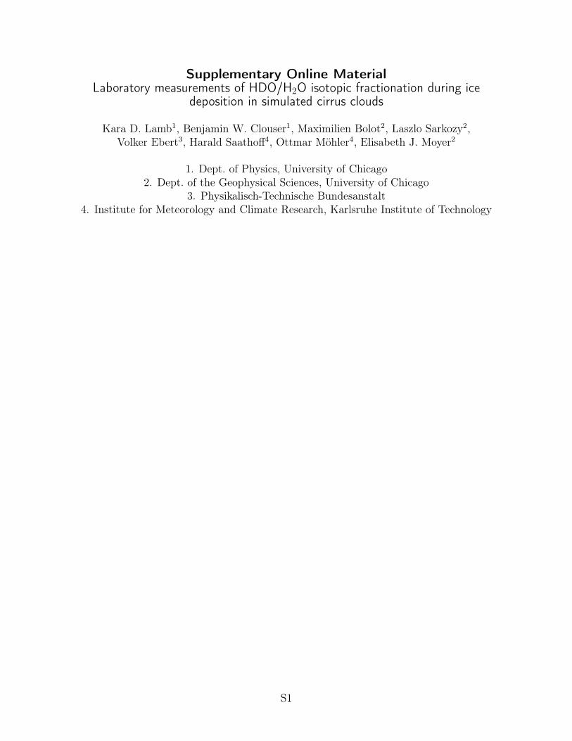
Figure S6: Cartoon demonstrating the effects ofdiffusion limitation on isotopic fractionation dur-ing ice growth. When diffusion becomes limiting,the effective fractionation becomes lower than inthe equilibrium case because vapour isotopic com-position is lower in the near field than in the bulkgas. This isotopic gradient arises primarily throughtwo mechanisms: preferential uptake of the heav-ier isotopologue (↵eq) and lower diffusivity of theheavier isotopologue (d). In more complex models,differences in deposition coefficients between iso-topologues can also play a role. See S6 for furtherdiscussion.

S15

S4 Fitting protocol: individual experiments

S4.1 Region selection

To determine the isotopic fractionation factor, it is important to select a region of theexperiment where the deposition of vapour as ice is maximal and the wall contribution isminimal, since the isotopic composition of the wall contribution is an unknown that weare approximating as constant. Most ice growth occurs in the first few minutes of eachexperiment, while outgassing from the chamber walls becomes progressively more importantas the experiment proceeds. Restricting the analyzed region to a segment near the beginningof each experiment therefore maximizes signal from the isotopic fractionation and minimizescontributions from the wall: the two terms on the right side of Eq. (4). For each experiment(defined as beginning at the onset of pumping) we select the analysis region using the criteria:Beginning

• At least 2% of the initial vapour must have deposited as ice• The isotopic ratio must have changed by at least 0.5% of its initial value

End• The outgassing rate must be less than or equal to the ice deposition rate• The cumulative flux from the chamber walls must be less than 15% of the initial vapour

Regions selected based on these criteria range from 54 to 223 seconds long, with a meanlength of 136 seconds. Region start times begin between 30 and 200 seconds after the onsetof pumping, so that the analysis region does not include the first several degrees of cooling.Start times are later at the coldest temperatures because of higher nucleation thresholds andslower rates of ice growth.

S4.2 Model implementation

The fractionation factors are estimated for each pumpdown by minimizing the differencebetween observed and modeled vapour isotopic ratios, with the isotopic ratios modeled ac-cording to Eq. (4). To arrive at a closed form solution, we parametrize ↵

eq

and � as follows:

• equilibrium fractionation factor: ↵

eq

= ↵

0

+

@↵eq

@T

����0

(T � T

0

), where T

0

is the tem-

perature at the beginning of the pumpdown. This linearization is acceptable becausethe variation in ↵

eq

over the course of each pumpdown is expected to be a small frac-tion of the dynamic range of ↵

eq

over all pumpdowns. Temperature changes duringpumpdowns are of order 5-9 K (2-5 K for regions analyzed), producing change in ↵

eq

of less than ⇠ 5%). This parameterization introduces a dependence of ↵eq

on the un-known @↵eq

@T

and so mandates an iterative solution: we start from an initial guess of@↵eq

@T

, solve for ↵0

in individual experiments, fit for the global temperature dependence,update @↵eq

@T

based on that solution, and iterate to convergence.

S16

• relative isotopic enrichment of outgassing vapour: � = R

w

/R

v

, with R

v

themeasured vapour isotopic composition, and R

w

the isotopic composition of wall out-gassing assumed constant during the analyzed period of each experiment. In reality thecomposition of the ice layers coating the chamber walls may show some structure, butthe outgassing composition likely varies sufficiently slowly to justify its approximationas constant. We set the constant R

w

in two ways:

– 2-parameter fit: We fit R

w

as a free parameter independent from ↵

eq

. Inpractice, the pumpdowns do not contain sufficient information to fully constrainR

w

and ↵

eq

separately, and the fitted values of the two variables are correlated.We use this fit as a reality check on results, and to estimate error bars on ↵

eq

forindividual experiments.

– 1-parameter fit: R

w

= ↵

eq

· Rv0

. We assume the wall outgassing compositionis that of an ice layer in equilibrium with chamber vapour before the pumpdown.R

w

is then tied to the equilibrium fractionation factor ↵

eq

and the measuredpre-pumpdown isotopic ratio in chamber vapour R

v0

. Data points in manuscriptFigure 2 and stated coefficients for ↵

eq

are taken from this fit.

Treatment of other model variables. While we fit on the raw 1-second measurements ofisotopic ratio, we use an effectively smoothed version of the measured evolving water vapourand total water to compute the terms P

vi

/r

v

and S

wv

/r

v

in Eq. (4). That is, we take thelow-order trend by computing the lowest SSA eigenmodes of the relevant measured timeseries ([29], see S4.4 for further discussion of SSA method). The modeled evolution of theisotopic ratio of vapour in the chamber is then determined by integrating Eq. (4) using aRunge-Kutta method with adaptative stepsize control, and the modeled isotopic ratio is fitto the raw measured isotopic ratio as described in the next section.

S4.3 Parameter and uncertainty estimation

We estimate parameters by the method of maximum likelihood. We denote the vector ofparameters to estimate as ✓. In the 2-parameter fit, ✓ = [✓

1

, ✓

2

]

T with ✓

1

= ↵

0

and ✓

2

= �

0

.In the 1-parameter fit, ✓ = [✓

1

] with ✓

1

= ↵

0

.Measured and modeled isotopic ratios are related as follows:

Robs

= Rm

(✓) + " (8)

where Robs are measured and Rm modeled isotopic ratios and " are inferred measurementerrors, discussed in S4.4. Because the errors are reasonably independent and normally dis-tributed, the likelihood of ✓ (that is, the probability of observing Robs given ✓) can be writtenas:

L (✓) = p

�Robs|✓

�

=

1

(2⇡)

N2p

det (C")

⇥ exp

�1

2

�Robs �Rm

(✓)�T

C�1

"

�Robs �Rm

(✓)��

(9)

S17

where N is the dimension of Robs (or Rm) and C" = E

⇥""T

⇤= diag (�

2

i

) is the covariancematrix of measurement errors. (See S4.4 for discussion of estimating measurement error �

i

.)The maximum likelihood estimator of ✓ is then the value ˆ✓ that maximizes L (✓). (We usethe “hat” symbol throughout to denote an estimated quantity.) In practice, we minimize�L (✓) = � logL (✓), which is equivalent to minimizing the following quantity:

1

2

NX

i=1

✓R

obs

i

�R

m

i

(✓)

�

i

◆2

(10)

The minimization of �L (✓) is carried out using a quasi-Newton algorithm.Uncertainty in retrieved parameters ✓ is estimated using Fisher matrix theory. The

likelihood L (✓) is asymptotically Gaussian near its maximum, i.e. it can be written:

L (✓) / exp

�1

2

⇣✓ � ˆ✓

⌘T

C�1

✓

⇣✓ � ˆ✓

⌘�(11)

where C✓ is the covariance matrix of the estimated parameters. (The inverse of C✓ is calledthe Fisher information matrix.) C✓ is computed as the inverse of the Hessian of the log-likelihood:

C✓ = � (r✓✓L)�1

= � (r✓✓ logL)�1 (12)

(The Hessian matrix is computed using centered finite differences.) The diagonal of C✓ thencontains the variance estimates of the parameters ✓

i

. That is, C✓ produces an estimate of theuncertainty �

↵

n

in each retrieval of an equilibrium fractionation factor ↵n

. These uncertaintiesare shown as the 2� error bars in Figure S1 and manuscript Figure 4.

Comparison of the estimated �

↵

n

for individual experiments and the distribution of derivedfractionation factors ↵

n

around the fit to all experiments suggests that these error estimatesare appropriate for the low-temperature experiments, in which signal-to-noise is the dominantfactor driving uncertainty, but are underestimates for the warmer experiments (T> 210 K),in which un-modeled systematic errors (likely driven by chamber inhomogeneities) dominate.We do not attempt to estimate additional contributions to experimental error, but note thattrue uncertainties may be a factor of three larger at the warmer end of the experimentaltemperature range.

S4.4 Measurement error estimation

The likelihood function used to estimate parameters for each pumpdown (Eq. 10) requiresan estimation of the intrinsic uncertainty �

i

in the isotopic ratio measurements. Determiningthis uncertainty would be trivial if its only source were measurement precision and instru-ment characteristics were fixed; in this case measurement errors could simply be estimatedfrom instrument performance in static conditions. Error estimation during pumpdowns ismore challenging because instrument performance can be altered by vibrations and attenua-tion of signal, and because chamber inhomogeneities increase during pumpdowns. Effectivemeasurement errors are therefore not constant during experiments. Since we are interestedin changes in isotopic ratio rather than absolute changes in concentrations, uncertainties inspectroscopic parameters and most other factors affecting accuracy do not affect results.

S18

lag [s]-50 0 50

cova

rianc

e

-1

0

1

2

3

4

5

6

ε/σ-5 -1 1 5

dens

ity

0

0.05

0.1

0.15

0.2

0.25

0.3

0.35

0.4

t [s]100 200 300

ε(t),σ(t)

-0.05

0

0.05ϵ

σ

Figure S7: Example of estimated noise on isotopic ratio measurements for experiment #6. Left: Thereconstructed noise from the trailing SSA eigenmodes and their associated standard deviation. Note thatnoise grows over the course of the pumpdown. Center: The standardized error is reasonably normallydistributed. Right: The reconstructed noise is reasonably decorrellated in time.

To estimate effective measurement error in a timeseries of isotopic ratio measurements, weassume that the effective error is manifested as deviations from a smoothly evolving isotopicratio. While the fit for ↵

n

is performed on raw isotopic measurements, we estimate errorsby taking a Singular Spectrum Analysis (SSA) [29] on that raw timeseries. SSA decomposesthe timeseries into a sum of eigenmodes (temporal principal components), each of themaccounting in decreasing order for a fraction of the variance of the original time series. Weuse the first few leading eigenmodes to construct the assumed smoothly evolving timeseries,and consider the trailing eigenmodes to represent the noise "

i

on the measured isotopic ratio.The rank at which we set this eigenmode separation is determined by the test that errorsmust be reasonably time-decorrelated.

Note that this method cannot distinguish one important experimental artifact: low-frequency fluctuations due to chamber inhomogeneities, which are correlated in time. Iso-topic measurements probe only the volume intersected by our infrared laser beam; chamberair circulating across the beam path results in small but important real fluctuations in tem-perature, water vapour content, and ice crystal number density, with timescale ⇠ 30 s.

Because effective noise characteristics change during a pumpdown (Fig. S7, left), wecannot simply take measurement uncertainty as the sample standard deviation of the noise"

i

, but instead must construct a standard error �i

that changes over the i datapoints of thepumpdown. For this estimation, we use the fact that the noise covariance matrix E

⇥""T

⇤=

diag (�

2

i

), so that �2

i

can be taken as the leading SSA eigenmode of the "

2

i

time series.We then test the validity of our approach for estimating "

i

and associated standarddeviation �

i

by checking the distribution of the standardized errors "i

/�

i

in each pumpdown.Because our approach models the likelihood of our parameters as a multivariate normaldistribution of variance �

i

, values of "i

/�

i

during a pumpdown should be normally distributedwith variance 1 and decorrelated in time. We find that they are indeed sufficiently wellbehaved with respect to our basic assumptions (Fig. S7). In the next section, we find thatthe �

i

are also optimal, in the sense that rescaling only marginally improves likelihoods.

S19

S4.4.1 Error rescaling

As a check on our error estimation procedure, we also test the possibility that the covariancematrix of measurement errors C" previously derived is known only up to a scaling factor.That is, we consider whether the standard deviations of measurement errors may in fact bes�

i

, where s is a global scaling factor attached to each pumpdown. In that case, C" wouldbe known up to s

2. In the previous section, we assumed s = 1. We now determine s bytreating it as one of the parameters estimated by maximizing the likelihood function. Forinstance, with ✓

1

= ↵

0

and ✓

2

= �

0

, we set ✓3

= s. The minimization of �L (✓) = � logL (✓)is now equivalent to minimizing the quantity:

NX

i=1

log (✓

3

�

i

) +

1

2

NX

i=1

✓R

obs

i

�R

m

i

(✓

1

, ✓

2

)

✓

3

�

i

◆2

. (13)

As can be seen in Fig. S8, rescaling the errors improves the likelihood only marginally,meaning this operation is essentially superfluous for estimating the fractionation factors andtheir associated standard errors. These results imply that the characterization of errorsdescribed in Sec. S4.4 is already nearly optimal and cannot be much improved.

Experiment #

0 5 10 15 20 25 30 35 40 45 50

sca

ling

fa

cto

r

0

0.5

1

1.5

Figure S8: The derived scaling factor s for error for all experiments fits to close to 1, demonstrating thatthe noise reconstruction from the SSA eigenmodes provides a good estimation of the covariance matrix ofmeasurement errors (likelihood is only marginally improved by rescaling). This means that the uncertainty on↵0

for individual pumpdowns is sufficiently well-estimated using the minimization of the likelihood functionwithout the inclusion of an additional scaling factor.

S5 Fitting protocol: temperature dependence

S5.1 Global fit procedure

After repeating the estimation procedure described above (S4.3) for all n experiments toobtain individual estimates for the fractionation factors ↵

n

at temperatures T

n

, and corre-

S20

sponding uncertainties �↵

n

, we then fit for the temperature dependence of ↵eq

, assuming thatit follows the form:

log↵

eq

= a

0

+

a

1

T

2

(14)

A 1/T

2 temperature dependence was also assumed in the M67 parameterization [4].Eq. 14 stems from quantum mechanical considerations [2, 30], and is derived by expand-

ing the partition functions for isotopically substituted and non-substituted species under theharmonic approximation for the force field potentials. A more general form including theeffects of anharmonicity would be:

log↵

eq

= �

0

+

�

1

T

+

�

2

T

2

(15)

In most isotopic systems, the anharmonic term �

1

/T can be neglected at high temperatures[31], but in the case of hydrogen partitioning the effects of anharmonicity and non-classicalrotation are important. It is not straightforward to determine the appropriate functionalform for the isotopic fractionation factor for HDO to H

2

O, but our measurements suggestthat Eq. (14) sufficiently represents the functional relationship, since the experimentallyderived values for the fractionation factor for individual pumpdowns appear roughly linearin log(↵

eq

) vs. 1/T

2 space.To provide consistency with previously measured values for the fractionation factor at

higher temperatures, which agree well, we further impose the constraint that we take thehighest temperature measurement from [4] to be a true value, fixing ↵

0

= 1.143 at T

0

=

�6

�C. This constraint does not significantly affect the parameterization of ↵eq over our

experimental temperature range.To estimate the temperature dependence, we make Eq. (14) linear with a change of

variables to x = log↵

eq

and t = 1/T

2: x = a

0

+ a

1

t.Including the constraint at T

0

then yields:

x� x

0

= a

1

(t� t

0

) (16)

and estimating the temperature dependence �

1

becomes a linear estimation problem:

x� x0 = H · a1

+w (17)

where x� x0 describes fractionation values derived for individual experiments: x� x0 =

[0, x

1

� x

0

, ..., x

N

� x

0

]

T , and H the experimental temperatures: H = [0, t

1

� t

0

, ..., t

N

� t

0

]

T .w is the vector of errors on the determination of log↵

eq

; the covariance matrix of w isCw = diag

⇥(�

↵

n

/↵

n

)

2

⇤. (See S4.3 for discussion of ↵

n

and �

↵

n

.) Following standard theory,the best linear estimator of a

1

is:

a

1

=

�HTC�1

w

H��1

HTC�1

w

· (x� x0) (18)

and its uncertainty is (�a1)

2

=

�HTC�1

w

H��1, which can be used to build confidence intervals.

Note that during the estimation procedure, Cw

is internally resized in order to bettermatch the dispersion of the residuals. That is, C

w

is rescaled by a factor such that thevariance of the standardized residuals becomes 1 (compensating for the underestimation ofuncertainties for individual experiments noted earlier).

S21

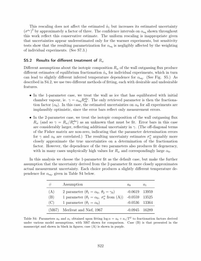
This rescaling does not affect the estimated a

1

but increases its estimated uncertainty(�

a1)

2 by approximately a factor of three. The confidence intervals on ↵

eq

shown throughoutthis work reflect this conservative estimate. The uniform rescaling is inappropriate giventhat uncertainties appear underestimated only for the warmer experiments, but sensitivitytests show that the resulting parametrization for ↵

eq

is negligibly affected by the weightingof individual experiments. (See S7.3.)

S5.2 Results for different treatment of R

w

Different assumptions about the isotopic composition R

w

of the wall outgassing flux producedifferent estimates of equilibrium fractionation ↵

n

for individual experiments, which in turncan lead to slightly different inferred temperature dependence for ↵

eq

. (See Fig. S5.) Asdescribed in S4.2, we use two different methods of fitting, each with desirable and undesirablefeatures.

• In the 1-parameter case, we treat the wall as ice that has equilibrated with initialchamber vapour, ie. � = ↵

eq

R

obs

v0

. The only retrieved parameter is then the fractiona-tion factor (↵

0

). In this case, the estimated uncertainties on ↵

0

for all experiments areimplausibly optimistic, since the error bars reflect only measurement errors.

• In the 2-parameter case, we treat the isotopic composition of the wall outgassing fluxR

w

(and so � = R

w

/R

obs

v

) as an unknown that must be fit. Error bars in this caseare considerably larger, reflecting additional uncertainty in �. (The off-diagonal termsof the Fisher matrix are non-zero, indicating that the parameter determination errorsfor � and ↵

0

are correlated.) The resulting uncertainty estimates �

↵

n

arguably moreclosely approximate the true uncertainties on a determination of the fractionationfactor. However, the dependence of the two parameters also produces fit degeneracy,with in many cases unphysically high values for R

w

and correspondingly large ↵

0

.

In this analysis we choose the 1-parameter fit as the default case, but make the furtherassumption that the uncertainty derived from the 2-parameter fit more closely approximatesactual measurement uncertainty. Each choice produces a slightly different temperature de-pendence for ↵

eq

, given in Table S4 below.

# Assumption a

0

a

1

(A) 2 parameter (✓1

= ↵

0

, ✓

2

= �

0

) -0.0619 13959(B) 1 parameter (✓

1

= ↵

0

, �

↵

n

from (A)) -0.0559 13525(C) 1 parameter (✓

1

= ↵

0

) -0.0536 13364

(M67) Merlivat and Nief, 1967 -0.0945 16289

Table S4: Parameters a0

and a1

obtained upon fitting log↵ = a0

+ a1

/T 2 to fractionation factors derivedunder various model assumptions, with M67 shown for comparison. Case (B) is that presented in themanuscript and shown in black in figures; case (A) is shown in purple.

S22

S6 Evaluation of kinetic models

Because the IsoCloud 4 experiments include a variety of mean supersaturations ¯

S

i

, condi-tions in which kinetic isotope effects should have differing influence, they allow testing thepredictions of different models for the kinetic modification to fractionation. In all cases, weassume that kinetic isotopic effects can be represented by Eq. (7), i.e.:

↵

k

=

S

i

↵eq · g (Si

� 1) + 1

We test the effect of different proposed values for the parameter g, which is a function ofd, the ratio of diffusivities of H

2

O and HDO, and, in some treatments, of surface effectsincluding the ratio of deposition coefficients between isotopologues.

S6.1 Kinetic fractionation models

We test two different treatments of kinetic isotopic effects.

Diffusive flux model: The default representation of kinetic modifications to fractionationin this work is the diffusive model of Jouzel and Merlivat [25], i.e. Eq. (7) with

g = d

Diffusive plus surface-kinetics model: Nelson [26] extends the diffusive flux model toinclude surface kinetic effects by setting

g = d · 1 + z

0

1 + z

where z = Z

S

/Z

V

is the ratio of the surface impedance to the vapour impedance, and asbefore, we denote quantities associated with the heavier isotopologue with a prime. If weassume spherical geometry for ice crystals, this expression can be rewritten as

g =

dk + yx1 + k

where x is the ratio of deposition coefficients for H2

O and HDO (x=�/�

0) and y is theirratio of thermal velocities (

p19/18). The coefficient k ⌘ rv�/ (4D

v

), where r is the icecrystal radius and v, �, and D

v

are the thermal velocity, deposition coefficient, and diffusioncoefficient in air, respectively, for the abundant isotopologue H

2

O. We make the simplifyingassumption that � = 1; the value is unknown but is likely of order 1 [32]. We take thetemperature- and pressure-dependent D

v

from Hall and Pruppacher 1976 [33]. In the limitk >> 1, the expression reduces to that of the diffusive model. In the experiments analyzedhere, values for k range from 2-15 across pumpdowns, essentially following the mean icecrystal diameter (2-14 µm). The greatest sensitivity to surface effects therefore occurs atthe lowest temperatures, where ice crystal size and k are smallest. The ratio of depositioncoefficients x is essentially unknown; Nelson [26] suggests that its value could plausibly liebetween 0.8 and 1.2.

S23

S6.2 Estimates of the isotopic diffusivity ratio

The value of d has been determined in a limited number of experiments, whose results areinconsistent within stated error bars. (Published values differ by as much as 3% while statederror bars are < 0.1%.) We summarize published results below in Table S5. In this work wetake as our default for d the value from Cappa et al. 2003 [34].

Kinetic isotope effects in our experiments are predominantly driven by equilibrium frac-tionation during ice deposition, with differences in diffusivity playing only a minor role. Inthe diffusive flux model for kinetic isotopic effects given above, d plays an identical role tothe equilibrium fractionation factor ↵

eq

: both appear only in the coefficient ↵eq

d, and whiled is only a few percent above 1, ↵

eq

is ⇠1.2-1.4 over the experimental temperature range.Nevertheless, uncertainty in d can still contribute significantly to uncertainty in kinetic ef-fects.

Measurement T (�C) T (K) DHDO/DH2O DH2O/DHDO (d)Ehhalt and Knott, 1965 [35] 20.0 293.2 0.9852± 0.003 1.0150Cappa et al., 2003 [34] 20.0 293.2 0.9839 1.0164Merlivat, 1978 [36] 21.0 294.2 0.9755± 0.0009 1.0251Luz et al., 2009 [37] -83.2 190.0 0.9573 1.0446– 10.0 283.2 0.9720± 0.0005 1.0288– 20.1 293.3 0.9775± 0.0005 1.0230– 39.8 313.0 0.9798± 0.0005 1.0206– 69.5 342.7 0.9841± 0.0003 1.0162

Table S5: Published estimates of the ratio of diffusivities for HDO and H2

O in air. Values from Cappa etal. are derived from kinetic theory and given without uncertainties. Values for Luz et al. in regular font aremeasurements; in italics is the value that would be extrapolated at 190 K by an unweighted linear fit to thesevalues: d=1.0807-1.901·10�4 · T , with T in Kelvin. (Only Luz et al. suggest a temperature dependence).

S6.3 Tests of kinetic models

We test the validity of models of the kinetic isotope effect by examining whether, aftercorrection for kinetic contributions to fractionation, the values for equilibrium fractionationretrieved from individual experiments (↵

n

) show dependence on supersaturation S

i

. A de-pendence on saturation would be interpreted as the signature of under- or over-correctionfor kinetic effects. Absence of a trend would suggest that the magnitude of kinetic effectshad been correctly estimated.

Because the experiments analyzed here are conducted at different temperatures, andequilibrium fractionation is a function of temperature, we do not consider the derived equi-librium fractionation factors ↵

n

directly. Instead, we consider their implied coefficients a

n

1

.Because the model for ↵eq is constrained to include a measured value at T = �6

�C, ourglobal fit for the temperature-dependent ↵eq can be fully described by this single coefficienta

1

. Similarly, each ↵

n

for an individual pumpdown defines a single a

n

1

that quantifies thetemperature dependence of the equilibrium fractionation factor that would be implied by

S24

that experiment alone. In M67, a1

is 16289. In our global fit, a1

is slightly lower, 13525. Ifall measurements were perfect, and the equilibrium fractionation factor exactly followed the1/T

2 dependence of Eq. (14), then each experiment would produce a

1

n exactly equal to thisa

1

. In reality, values of an1

derived from individual experiments scatter around this value.(See cartoon in Fig. S9.)

Figure S9: Cartoon to illustrate the slopes a1

n that appear in manuscript Figure 5 and Figure S10. a1

n isthe slope in log↵ vs. 1/T 2 space of the line connecting the assumed constraint point (1/T 2

0

, log(↵0

)) withan experimentally derived point (1/T 2, log(↵

n

)). Individual experiments in this work generally producea1

ns (slopes of dashed lines) below that of M67 (solid red) and therefore produce a weaker temperaturedependence for the globally fit ↵eq (solid black).

Any over- or under-correction for kinetic effects would produce a systematic trend inthe a

n

1

s with supersaturation S

i

. If g in the kinetic model is incorrectly specified (g 6=g

0

, where g

0

is the “true” value that would yield a perfect retrieval), then the resultingestimation of equilibrium fractionation ↵eq would be biased, and that bias would depend onsupersaturation:

@↵eq

@S

i

= (g � g

0

)↵

2

eq (19)

This expression can be rewritten in terms of a1

since

ln

↵eq

↵

0

= a

1

✓1

T

2

� 1

T

2

0

◆(20)

Combining equations 19 and 20 shows that @ ln a

1

/@S

i

is directly linked to the choice of g:

@ ln a

1

@S

i

= (g � g

0

)

↵eq

ln

⇣↵eq↵0

⌘, (21)

The absence of trend with S

i

would therefore suggest that kinetic effects have been modeledcorrectly, i.e. g = g

0

.

S25

We conduct two tests to determine the validity of kinetic models and establish constraintson the parameters d and x. While we cannot constrain d and x simultaneously, we canexamine their effects separately. First, we test a pure diffusive flux model (g = d) withdifferent values of d. We fit for the optimal value of the diffusivity ratio d that eliminatessupersaturation dependence, and determine bounds on potential values for d. We then testthe diffusive-plus-surface-kinetic model with d set at the default value of Cappa et al. [34],and determine an optimum value and bounds for x given that assumption. That is, we assumethat the value of the diffusivity ratio is known, and that any trend with saturation resultsfrom mis-estimation of surface kinetic effects due to an incorrect choice of the depositioncoefficient ratio x. In both cases we fit for the trend of a

1

ns vs. the deposition-weightedsupersaturation

¯

S

i

=

ZP

vi

S

i

/r

v

dt/

ZP

vi

/r

v

dt (22)

assuming a linear relationship: a1

(S

i

) = m ·Si

+b. We seek the value of g that yields zeroslope (m = 0) by using a root-finding algorithm, and estimate bounds as described below.As in the fit for ↵

eq

, we weight individual experiments by their uncertainty �

↵

n

(See S4).The results of these tests yield bounds on diffusivity and deposition coefficient ratios d and

x that are consistent with literature estimates of their plausible ranges. Manuscript Figure5 shows results of the test on d with the pure diffusive model. The implied optimal valueof d=1.01 is slightly lower than any measurement, but with bounds of ⇠ ±4% spanning thepublished values in Table S5: 0.97 < d < 1.05. Figure S10 shows results of the test on x withthe surface-kinetic model. Because the kinetic isotope effect is less sensitive to uncertaintyin x, the test provides a looser constraint, with bounds on x exceeding ±20%: 0.74 < x <1.17, spanning the range of 0.8-1.2 suggested by Nelson [26]. The central value of x=0.96would imply that HDO molecules were slightly more likely to be accommodated into thecrystal lattice than H

2

O, but results are also consistent with x=1.The looseness of these constraints stems from the small sample size of those IsoCloud

4 experiments sensitive to kinetic isotope effects. Only six experiments have deposition-weighted supersaturations above 1.2, three of those at temperatures low enough that signal-to-noise is poor and uncertainty in isotopic ratio measurements high. The small samplesize also means that individual outliers can strongly bias results. In this analysis, we omitexperiments #4, 26, and 48, three outlier experiments whose small nominal error bars leavethem inconsistent with the global derived ↵

eq

to greater than 5-� with respect to theirestimated uncertainties; including these experiments would substantially alter the derivedoptimal values for d and x. Even assuming the uncertainties are underestimated by 3x,all three experiments remain outliers, with 2.5-� residual with respect to their estimatederrors. Each of these experiments are also outliers with respect to the distribution in theirrespective temperature groups. The small sample size means that for d and x, IsoCloudresults should be considered suggestive rather than conclusive. These results do howeverconfirm the validity of kinetic models, and serve as a proof of concept of the approach.Future experimental campaigns targeted at kinetic isotope effects should be able to providestronger constraints.

To estimate bounds on kinetic isotope effect parameters, we evaluate uncertainty �

g

on estimating g

0

by propagating the uncertainty �slp on the slope @ ln a

1

/@S

i

. Becauseexperiments at different temperatures have different ↵

eq

, we know that uncertainty only to

S26

within some range. From Eq. (21), �g

must lie in the range:

�slp ·min{ln

⇣↵eq↵0

⌘

↵eq} �

g

�slp ·max{ln

⇣↵eq↵0

⌘

↵eq} (23)

where the min and max values are over all experiments in the analysis. When assumingthe diffusive model with g =d to obtain constraints on d, we conservatively take the upperlimit as the estimated uncertainty in d. When testing the surface-effect model with g =

(dk + yx) / (1 + k), to obtain constraints on x, we can rewrite Eq. (21) as:

@ ln a

1

@S

i

= (x� x

0

)

y

1 + k

↵eq

ln

⇣↵eq↵0

⌘ (24)

where x

0

is the value of x that would yield the “true” retrieval of ↵eq. The uncertainty �

x

onx

0

then satisfies the relationship:

�slp ·min{1 + k

y

ln

⇣↵eq↵0

⌘

↵eq} �

x

�slp ·max{1 + k

y

ln

⇣↵eq↵0

⌘

↵eq} , (25)

We again conservatively take the upper limit as our estimate of uncertainty in x

0

.

S27

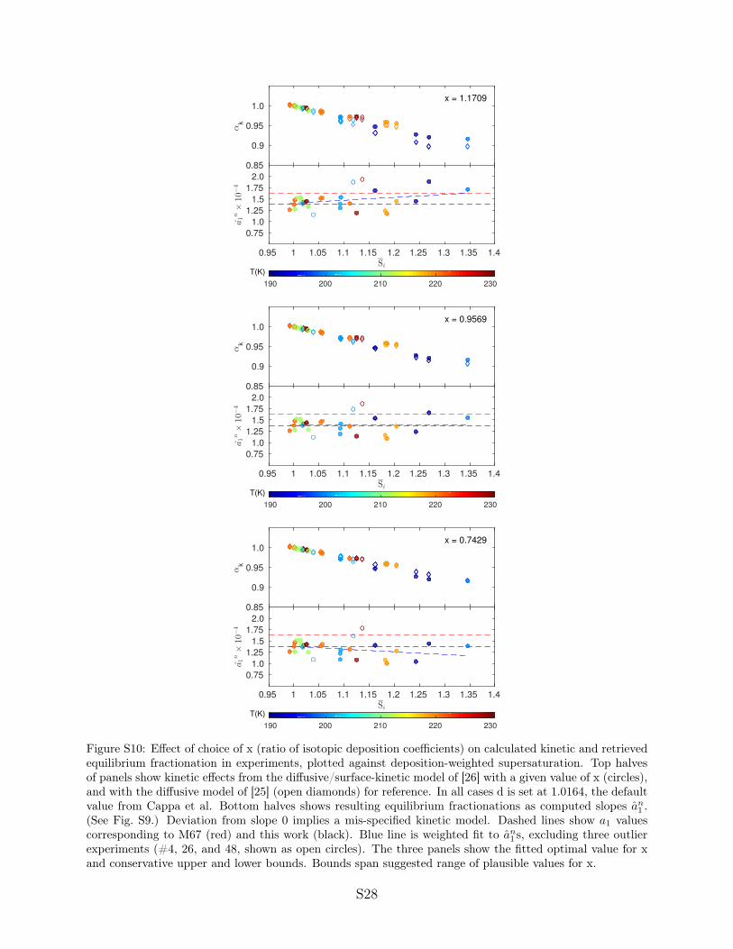
αk

0.85

0.9

0.95

1.0x = 1.1709

Si

0.95 1 1.05 1.1 1.15 1.2 1.25 1.3 1.35 1.4

a1n×10−4

0.75

1.0

1.25

1.5

1.75

2.0

190 200 210 220 230

T(K)

αk

0.85

0.9

0.95

1.0x = 0.9569

Si

0.95 1 1.05 1.1 1.15 1.2 1.25 1.3 1.35 1.4

a1n×10−4

0.75

1.0

1.25

1.5

1.75

2.0

190 200 210 220 230

T(K)

αk

0.85

0.9

0.95

1.0x = 0.7429

Si

0.95 1 1.05 1.1 1.15 1.2 1.25 1.3 1.35 1.4

a1n×10−4

0.75

1.0

1.25

1.5

1.75

2.0

190 200 210 220 230

T(K)

Figure S10: Effect of choice of x (ratio of isotopic deposition coefficients) on calculated kinetic and retrievedequilibrium fractionation in experiments, plotted against deposition-weighted supersaturation. Top halvesof panels show kinetic effects from the diffusive/surface-kinetic model of [26] with a given value of x (circles),and with the diffusive model of [25] (open diamonds) for reference. In all cases d is set at 1.0164, the defaultvalue from Cappa et al. Bottom halves shows resulting equilibrium fractionations as computed slopes an

1

.(See Fig. S9.) Deviation from slope 0 implies a mis-specified kinetic model. Dashed lines show a

1

valuescorresponding to M67 (red) and this work (black). Blue line is weighted fit to an

1

s, excluding three outlierexperiments (#4, 26, and 48, shown as open circles). The three panels show the fitted optimal value for xand conservative upper and lower bounds. Bounds span suggested range of plausible values for x.

S28

S7 Sensitivity tests on determination of ↵

eq

We perform several tests to evaluate the robustness of our determination of ↵eq

. We test forsensitivity to model assumptions (values for d), to measurement uncertainties (experimentalregion selection and bias in measured H

2

O), and to fitting procedure (weighting of experi-ments in global fit). All factors produce relatively minor changes, and retain the finding of↵

eq

below M67.

S7.1 Sensitivity to region choice

In all analyses described previously, we choose the experimental region analyzed for eachpumpdown by a set of fixed criteria, described in S4:

• that ice deposition rate exceeds wall outgassing: ✏ = S

wv

/P

vi

< 1

• that cumulative ice deposition exceeds a fraction � of initial vapour, with � = .02

• that the isotopic ratio has dropped by a fraction � from its initial value, with � = 0.005

The choice of region length can affect derived values of equilibrium fractionation forindividual experiments (↵

n

) and therefore global fits for ↵

eq

, for several reasons. As dis-cussed previously, wall outgassing isotopic composition is assumed constant but may showsome trend over time. More importantly, chamber inhomogeneities produce fluctuations inmeasured quantities with timescales ⇠30 s. With our region selection criteria, the timeseriesanalyzed for each pumpdown may contain 2-8 cycles of statistically significant fluctuations inmeasured quantities that affect ↵

n

. Default values for ✏, �, and � were chosen such that de-rived values for ↵

n

are relatively stable to moderate extensions or reductions of region length.We evaluate here sensitivity to these parameter choices by performing a Bayesian analysis.We allow ✏, �, and � to vary arbitrarily (within bounds ✏ 2 [0.3, 2.0], � 2 [0.01, 0.05] and� 2 [0.001, 0.01]), producing a wide range of candidate time segments. (In this analysis theregion choice is randomly chosen and all experiments are evaluated with the same choiceof parameters to define the region length.) We use each choice to derive an estimate for↵

eq

, and examine all results that meet goodness-of-fit criteria.1 Details of the analysis aredescribed at the end of this section.

While the region choice parameters can strongly affect a resulting global fit for ↵

eq

, wefind that the central value of the distribution of estimated a

1

in this analysis is very close tothat derived with the region choice algorithm of S4. That is, the most probable temperature-dependent ↵

eq

in the Bayesian analysis is consistent with the determination of ↵eq

in ourprevious analyses (Fig. S11). (The confidence interval derived from the Bayesian analysis

1Goodness of fit: We evaluate the goodness of the fit by: first, checking that the minimizer has

converged to a solution (r✓L ⇡ 0 to specified tolerance and r✓✓L positive definite); second, inspecting thenormalized residuals

Robs

i

�Rm

i

(✓)

�i

and checking that their distribution does not significantly deviate from a Gaussian with mean 0 and variance 1(to ensure compliance with Eq. (11)). This is assessed by a Kolmogorov-Smirnov test with a 5% significancelevel. Only fits to the randomly chosen regions which pass the goodness of fit test are included in theprobability distribution.

S29

is also smaller than that determined by the uncertainty analysis described in S5.) Theseresults suggest that our region choice criteria have not biased our estimation of ↵

eq

.

Figure S11: Test of sensitivity of global fit to region choice for individual experiments. We randomly varyparameters that determine the experiment region, then calculate the best global fit as described in thetext (using a 2-parameter fit). The expectation value of the resulting probability distribution is shownin green. Gray shaded region is the 99.73% confidence interval derived from the probability distribution.Results suggest that our region choice has not introduced systematic bias. The Bayesian best estimate givesa0

= �0.0649 and a1

= 14171, which is very close to the best 2-parameter fit with the region choice used inthe analysis. (In this test we take d from Merlivat, 1978, but d negligibly affects results; see S7.2 below.)

Bayesian analysis methods: The estimator of a1

computed in Eq. (18) implicitly dependson the chosen values of ✏, �, and � and can be seen as deterministic when these parametersare fixed. In this analysis we treat a

1

as a random variable with a PDF related to probabilitydistributions of ✏, �, and �:

p (a

1

) =

ZZZ+1

�1p (a

1

|✏,�,�) p (✏,�,�) d✏ d� d�

=

ZZZ+1

�1� (a

1

� a

1

(✏,�,�)) p (✏,�,�) d✏ d� d� (26)

where � represents the Dirac distribution. If ✏, �, and � are independent and uniformlydistributed between bounds, we can draw n samples (with n sufficiently large; we use n =

100) and evaluate the density of a1

as:

p (a

1

) ⇡ 1

n

nX

k=1

� (a1

� a

1

(✏

k

,�

k

,�

k

)) (27)

S30

or, more conveniently, to give a continuous representation of the density:

p (a

1

) ⇡ 1

n

nX

k=1

G (a

1

� a

1

(✏

k

,�

k

,�

k

)) (28)

where G is a Gaussian kernel of suitable width. The most probable a

1

and confidenceintervals on the estimate can then be computed from the probability distribution p (a

1

).

S7.2 Sensitivity to estimation of kinetic isotope effects

In this section we test the robustness of our estimation of ↵eq

to uncertainties that affect thecalculated kinetic modification to fractionation: uncertainty in the isotopic diffusivity ratiod and potential systematic bias in the measurement of H

2

O. Resulting errors in calculatedkinetic effects could affect the global estimate of ↵

eq

.

Isotopic diffusivity ratio (d)In section S6, we showed that different assumed values of d could significantly alter theslope of inferred ↵

n

against supersaturation. Those changes have a much smaller effecton the global fit for ↵

eq

, because the global fit of the IsoCloud 4 dataset is dominated byexperiments with small supersaturations and minimal kinetic effects. Varying d over therange of published estimates (⇠3% variation, see Table S5) can affect estimation of ↵

n

inindividual experiments by as much as 1-2% (Figure S12), but has virtually no effect on theretrieval of ↵

eq

, producing a maximum change of 0.02%. (We do not show a figure for thistest because the differences in ↵

eq

are too small to be visible by eye.) Uncertainty in dtherefore cannot bias our estimate of ↵

eq

.

185 190 195 200 205 210 215 220 225 230 235−0.025

−0.02

−0.015

−0.01

−0.005

0

0.005

0.01

0.015

0.02

0.025

Temperature (K)

∆ α

eq/α

eq

Cappa, 2003Ehhalt, 1965Luz, 2009

Figure S12: Effect of choices forthe isotopic diffusivity ratio d oninferred ↵

n

for individual exper-iments. We use the value of dfrom Merlivat 1978 as the refer-ence and show differences when dis taken instead from Cappa etal. 2003 (blue), Ehhalt and Knott1965 (green), and Luz et al. 2009(red). Individual experiments maybe affected by up to 1-2% , but theglobal fit for the temperature de-pendence of ↵

eq

must intersect thecluster of near-equilibrium experi-ments at ⇠210 K that show negli-gible dependence on d.

S31

SupersaturationSystematic bias in H

2

O measurements can affect estimates of isotopic fractionation in severalways: by changing the inferred ice deposition rate, and by producing a biased measurementof supersaturation S

i

and so a biased calculation of the kinetic modification to fractionation.The latter effect is by far the most important. Systematic measurement bias is common formeasurements of gas-phase species by absorption spectroscopy that do not involve empiricalcalibration, since spectral line parameters are not perfectly known. For the ChiWIS H

2

Omeasurements, stated uncertainties on line parameters from the HITRAN database [14,15] nominally limit the water vapour retrieval to an accuracy of ±5%. However, ChiWISmeasured vapour pressure in dense ice clouds, when water vapour should be drawn downto saturation, suggests that ChiWIS H

2

O measurements are accurate to within �1% and+2%. (These limits are 2 standard deviations around the mean of calculated ChiWIS S

i

,using [38] for saturation vapour pressure.) Potential biases of this magnitude would producenoticeable changes in estimated ↵

eq

, since experiments at S

i

⇠ 1 would then be assumed toexperience super- or sub-saturation and kinetic modifications to fractionation. The effect isshown in Fig. S13. Systematic over- or under-estimation of supersaturation is the largestsource of systematic uncertainty in our analysis. However, the range of potential changesremains within the 3� confidence interval of the best fit presented here.

Figure S13: Sensitivity of fit for ↵eq

to potential fractional bias in water vapour and therefore Si

. Black lineshows default best-fit ↵

eq

; grey lines repeat analysis with assumption that ChiWIS H2

O has bias of +2% and�1%. Overestimating H

2

O would lead to overestimating kinetic modification to fractionation and so ↵eq

;the true value of ↵

eq

would then be lower than estimated. Similary, underestimating H2

O would mean thetrue value of ↵

eq

would be higher than estimated. Gray shaded region is the 3� confidence interval describedpreviously.

S32

S7.3 Sensitivity to weights on individual experiments

As mentioned previously, our estimated experimental uncertainties may be subject to temperature-dependent bias. The global fit procedure, which weights individual experiments by theirestimated error, may therefore over-weight the warm-temperature experiments relative tothose at T < 210 K. We test for any resulting bias in determination of ↵

eq

by comparingto a fit with all experiments treated equally. The parametrizations for ↵

eq

in the weightedand unweighted fits are not significantly different (Figure S14). (The parameters in the un-weighted fit are a

0

= -0.0595 and a

1

=13837; compare to values in Table S4.) Our estimateof ↵

eq

appears robust to errors in the weighting of individual experiments.

Temperature (K)180 190 200 210 220 230 240 250 260 270

αe

q

1.15

1.2

1.25

1.3

1.35

1.4

1.45

1.5

1.55

1.6Merlivat, 1967Ellehoj, 2013this work (1 param.)this work (2 param.)this work (unweighted)

Figure S14: Sensitivity of the fit for ↵eq

to potential uncertainty in the weighting of individual experiments.Black line shows default best-fit ↵

eq

using weights derived from the uncertainty analysis; green line repeatsthe analysis with equal weighting for all experiments. Gray shaded region is the 3� confidence intervaldescribed previously.

S33

References

[1] J. Bigeleisen. Statistical mechanics of isotopic systems with small quantum corrections.I. General considerations and the rule of the geometric mean. The Journal of ChemicalPhysics, 23(12):2264–2267, 1955.

[2] H. C. Urey. The thermodynamic properties of isotopic substances. J. Chem. Soc., pages562–581, 1947.

[3] S. Matsuo, H. Kuniyoshi, and Y. Miyake. Vapor pressure of ice containing D2

O. Science,145(3639):1454–1455, 1964.

[4] L. Merlivat and G. Nief. Fractionnement isotopique lors des changements d’état solide-vapeur et liquide-vapeur de l’eau à des températures inférieures 0�C. Tellus, 19(1):122–127, 1967.

[5] W. A. Van Hook. Vapor pressures of the isotopic waters and ices. The Journal ofPhysical Chemistry, 72(4):1234–1244, 1968.

[6] M. Johansson and K. Holmberg. Separation of heavy water in phase equilibria involvingpure water or salt-water systems. Acta Chemica Scandinavica, 23:765–781, 1969.

[7] J. D. Pupezin, G. Jakli, G. Jancso, and W. A. Van Hook. Vapor pressure isotopeeffect in aqueous systems. I. water-water-D2 (-64.deg. to 100.deg.) and water-water18-O (-17.deg. to 16.deg.). Ice and liquid. II. Alkali metal chloride solution in water andwater-D2 (-5.deg. to 100.deg.). The Journal of Physical Chemistry, 76(5):743–762, 1972.

[8] M. Méheut, M. Lazzeri, E. Balan, and F. Mauri. Equilibrium isotopic fractionation inthe kaolinite, quartz, water system: Prediction from first-principles density-functionaltheory. Geochimica et Cosmochimica Acta, 71(13):3170–3181, 2007.

[9] M. D. Ellehøj, H. C. Steen-Larsen, S. J. Johnsen, and M. B. Madsen. Ice-vapor equilib-rium fractionation factor of hydrogen and oxygen isotopes: Experimental investigationsand implications for stable water isotope studies. Rapid Communications in Mass Spec-trometry, 27(19):2149–2158, 2013.

[10] C. Pinilla, M. Blanchard, E. Balan, G. Ferlat, R. Vuilleumier, and F. Mauri. Equilibriumfractionation of H and O isotopes in water from path integral molecular dynamics.Gechemica et Cosmochimica Acta, 135:203–216, 2014.

[11] O. Möhler, O. Stetzer, S. Schaefers, C. Linke, M. Schnaiter, R. Tiede, H. Saathoff,M. Krämer, A. Mangold, P. Budz, P. Zink, J. Schreiner, K. Mauersberger, W. Haag,B. Kärcher, and U. Schurath. Experimental investigation of homogeneous freezing ofsulphuric acid particles in the aerosol chamber aida. Atmos. Chem. Phys., 3:211–223,2003.

[12] C. Lauer. Aufbau und Validierung eines kalibrationsfreien, extraktiven 1.4 um-Laserhygrometers für den Einsatz an der Aerosolkammer AIDA. PhD thesis, 2007.

S34

[13] J. Skrotzki. High-accuracy multiphase humidity measurements using TDLAS: applica-tion to the investigation of ice growth in simulated cirrus clouds. PhD thesis, 2012.

[14] L. S. Rothman, D. Jacquemart, A. Barbe, D. C. Benner, M. Birk, L. R. Brown, M. R.Carleer, C. Chackerian, K. Chance, and L. H. et al. Coudert. The HITRAN 2004molecular spectroscopic database. Journal of Quantitative Spectroscopy and RadiativeTransfer, 96(2):139–204, 2005.

[15] L. S. Rothman, I. E. Gordon, A. Barbe, D. C. Benner, P. F. Bernath, M. Birk,V. Boudon, L. R. Brown, A. Campargue, and J.P. et al. Champion. The HITRAN2008 molecular spectroscopic database. Journal of Quantitative Spectroscopy and Ra-diative Transfer, 110(9):533–572, 2009.

[16] R. Wagner and O. Möhler. Heterogeneous ice nucleation ability of crystallinesodium chloride dihydrate particles. Journal of Geophysical Research: Atmospheres,118(10):4610–4622, 2013.

[17] O. Möhler, P. R. Field, P. Connolly, S. Benz, H. Saathoff, M. Schnaiter, R. Wagner,R. Cotton, M. Krämer, A. Mangold, and A. J. Heymsfield. Efficiency of the depositionof mode ice nucleation on mineral dust particles. Atmos. Chem. Phys., 6:3007–3021,2006.

[18] J. U. White. Long optical paths of large aperture. J. Opt. Soc. Am., 32(5):285–285,May 1942.

[19] J. U. White. Very long optical paths in air. JOSA, 66(5):411–416, 1976.

[20] L. Sarkozy, B. Clouser, K. Lamb, E. Stutz, H. Saathoff, V. Ebert, S. Wagner, B. Küh-nreich, and E. Moyer. TDL spectrometer for chamber-based isotopic measurements ofwater vapor isotopic evolution during cirrus formation. submitted to Review of ScientificInstruments, 2017.

[21] H. Craig. Isotopic variations in meteoric waters. Science, 133(3465):1702–1703, 1961.

[22] R. Hagemann, G. Nief, and E. Roth. Absolute isotopic scale for deuterium analysis ofnatural waters. Absolute D/H ratio for SMOW1. Tellus, 22(6):712–715, 1970.

[23] P. Baertschi. Absolute 18O content of standard mean ocean water. Earth and PlanetaryScience Letters, 31(3):341–344, 1976.

[24] R. J. Cotton, S. Benz, P.R. Field, O. Möhler, and M. Schnaiter. Technical note: A nu-merical test-bed for detailed ice nucleation studies in the aida cloud simulation chamber.Atmos. Chem. Phys., 7:243–256, 2007.

[25] J. Jouzel and L. Merlivat. Deuterium and oxygen 18 in precipitation: Modeling ofthe isotopic effects during snow formation. Journal of Geophysical Research, 89:11749–11757, 1984.

S35

[26] J. Nelson. Theory of isotopic fractionation on facetted ice crystals. Atmospheric Chem-istry and Physics, 11(22):11351–11360, 2011.

[27] M. Bolot, B. Legras, and E. J. Moyer. Modelling and interpreting the isotopic compo-sition of water vapour in convective updrafts. Atmos. Chem. Phys., 13(16):7903–7935,2013.

[28] D. A. Fisher. Remarks on the deuterium excess in precipitation in cold regions. TellusB, 43:401–407, 1991.

[29] M. Ghil, M. R. Allen, M. D. Dettinger, K. Ide, D. Kondrashov, M. E. Mann, A. W.Robertson, A. Saunders, Y. Tian, F. Varadi, and P. Yiou. Advanced spectral methodsfor climatic time series. Reviews of Geophysics, 40(1):3–1–3–41, 2002.

[30] J. Bigeleisen. Statistical Mechanics of Isotope Effects on the Thermodynamic Propertiesof Condensed Systems. The Journal of Chemical Physics, 34(5):1485–1493, 1961.

[31] R. E. Criss. Temperature dependence of isotopic fractionation factors. Stable IsotopeGeochemistry: A Tribute to Samuel Epstein, 3:11–16, 1991.

[32] J. Skrotzki, P. Connolly, M. Schaniter, H. Saathoff, O. Möhler, R. Wagner, M. Niemand,V. Ebert, and T. Leisner. The accommodation coefficent of water molecules on ice-cirruscloud studies at the aida simulation chamber. Atmos. Chem. Phys., 12:24351–24393,2012.

[33] W. D. Hall and H. R. Pruppacher. The survival of ice particles falling from cirrus cloudsin subsaturated air. Journal of the Atmospheric Sciences, 33(10):1995–2006, 1976.

[34] C. D. Cappa, M. B. Hendricks, D. J. DePaolo, and R. C. Cohen. Isotopic fractionationof water during evaporation. Journal of Geophysical Research: Atmospheres, 108(D16),2003.

[35] D. Von Ehhalt and K. Knott. Kinetische Isotopentrennung bei der Verdampfung vonWasser. Tellus, 17(3):389–397, 1965.

[36] L. Merlivat. Molecular diffusivities of H16

2

O, HD16O, and H18

2

O in gases. The Journalof Chemical Physics, 69(6):2864–2871, 1978.

[37] B. Luz, E. Barkan, R. Yam, and A. Shemesh. Fractionation of oxygen and hydrogenisotopes in evaporating water. Geochimica et Cosmochimica Acta, 73(22):6697–6703,2009.

[38] D. M. Murphy and T. Koop. Review of the vapour pressures of ice and supercooled waterfor atmospheric applications. Quarterly Journal of the Royal Meteorological Society,131(608):1539–1565, 2005.

S36

View publication statsView publication stats