Contents

Chapter 1 ( Introduction ) 3

Setup . . . . . . . . . . . . . . . . . . . . . . . . . . . . . . . . . . . . 4

Building with Stack (Recommended) . . . . . . . . . . . . . . . . 4

Building with Cabal . . . . . . . . . . . . . . . . . . . . . . . . . 5

Building with make . . . . . . . . . . . . . . . . . . . . . . . . . . 5

The Basic Language . . . . . . . . . . . . . . . . . . . . . . . . . . . . 5

LLVM Introduction . . . . . . . . . . . . . . . . . . . . . . . . . . . . 6

Full Source . . . . . . . . . . . . . . . . . . . . . . . . . . . . . . . . . 9

Chapter 2 (Parser and AST) 9

Parser Combinators . . . . . . . . . . . . . . . . . . . . . . . . . . . . 9

The Lexer . . . . . . . . . . . . . . . . . . . . . . . . . . . . . . . . . . 9

The Parser . . . . . . . . . . . . . . . . . . . . . . . . . . . . . . . . . 11

The REPL . . . . . . . . . . . . . . . . . . . . . . . . . . . . . . . . . 14

Full Source . . . . . . . . . . . . . . . . . . . . . . . . . . . . . . . . . 15

Chapter 3 ( Code Generation ) 15

Haskell LLVM Bindings . . . . . . . . . . . . . . . . . . . . . . . . . . 16

Code Generation Setup . . . . . . . . . . . . . . . . . . . . . . . . . . 16

Blocks . . . . . . . . . . . . . . . . . . . . . . . . . . . . . . . . . . . . 18

Instructions . . . . . . . . . . . . . . . . . . . . . . . . . . . . . . . . . 19

From AST to IR . . . . . . . . . . . . . . . . . . . . . . . . . . . . . . 22

Full Source . . . . . . . . . . . . . . . . . . . . . . . . . . . . . . . . . 25

Chapter 4 ( JIT and Optimizer Support ) 26

ASTs and Modules . . . . . . . . . . . . . . . . . . . . . . . . . . . . . 26

Constant Folding . . . . . . . . . . . . . . . . . . . . . . . . . . . . . . 27

Optimization Passes . . . . . . . . . . . . . . . . . . . . . . . . . . . . 28

Adding a JIT Compiler . . . . . . . . . . . . . . . . . . . . . . . . . . 30

External Functions . . . . . . . . . . . . . . . . . . . . . . . . . . . . . 31

Full Source . . . . . . . . . . . . . . . . . . . . . . . . . . . . . . . . . 33

1

Chapter 5 ( Control Flow ) 34

‘if’ Expressions . . . . . . . . . . . . . . . . . . . . . . . . . . . . . . . 34

‘for’ Loop Expressions . . . . . . . . . . . . . . . . . . . . . . . . . . . 40

Full Source . . . . . . . . . . . . . . . . . . . . . . . . . . . . . . . . . 45

Chapter 6 ( Operators ) 45

User-defined Operators . . . . . . . . . . . . . . . . . . . . . . . . . . . 45

Binary Operators . . . . . . . . . . . . . . . . . . . . . . . . . . . . . . 46

Unary Operators . . . . . . . . . . . . . . . . . . . . . . . . . . . . . . 48

Kicking the Tires . . . . . . . . . . . . . . . . . . . . . . . . . . . . . . 49

Full Source . . . . . . . . . . . . . . . . . . . . . . . . . . . . . . . . . 54

Chapter 7 ( Mutable Variables ) 54

Why is this a hard problem? . . . . . . . . . . . . . . . . . . . . . . . 55

Memory in LLVM . . . . . . . . . . . . . . . . . . . . . . . . . . . . . 57

Mutable Variables . . . . . . . . . . . . . . . . . . . . . . . . . . . . . 60

Assignment . . . . . . . . . . . . . . . . . . . . . . . . . . . . . . . . . 62

Full Source . . . . . . . . . . . . . . . . . . . . . . . . . . . . . . . . . 64

Chapter 8 ( Conclusion ) 64

Tutorial Conclusion . . . . . . . . . . . . . . . . . . . . . . . . . . . . 64

Chapter 9 ( Appendix ) 66

Command Line Tools . . . . . . . . . . . . . . . . . . . . . . . . . . . 66

Adapted by Stephen Diehl ( @smdiehl )

This is an open source project hosted on Github. Corrections and feedbackalways welcome.

• Version 1: December 25, 2013• Version 2: May 8, 2017

The written text licensed under the LLVM License and is adapted from theoriginal LLVM documentation. The new Haskell source is released under theMIT license.

2

Chapter 1 ( Introduction )

Welcome to the Haskell version of “Implementing a language with LLVM” tutorial.This tutorial runs through the implementation of a simple language, and thebasics of how to build a compiler in Haskell, showing how fun and easy it can be.This tutorial will get you up and started as well as help to build a frameworkyou can extend to other languages. The code in this tutorial can also be used asa playground to hack on other LLVM specific things. This tutorial is the Haskellport of the C++, Python and OCaml Kaleidoscope tutorials. Although mostof the original meaning of the tutorial is preserved, most of the text has beenrewritten to incorporate Haskell.An intermediate knowledge of Haskell is required. We will make heavy use ofmonads and transformers without pause for exposition. If you are not familiarwith monads, applicatives and transformers then it is best to learn these topicsbefore proceeding. Conversely if you are an advanced Haskeller you may noticethe lack of modern techniques which could drastically simplify our code. Insteadwe will shy away from advanced patterns since the purpose is to instruct inLLVM and not Haskell programming. Whenever possible we will avoid clevernessand just do the “stupid thing”.The overall goal of this tutorial is to progressively unveil our language, describinghow it is built up over time. This will let us cover a fairly broad range of languagedesign and LLVM-specific usage issues, showing and explaining the code for itall along the way, without overwhelming you with tons of details up front.It is useful to point out ahead of time that this tutorial is really about teachingcompiler techniques and LLVM specifically, not about teaching modern and sanesoftware engineering principles. In practice, this means that we’ll take a numberof shortcuts to simplify the exposition. If you dig in and use the code as a basisfor future projects, fixing these deficiencies shouldn’t be hard.I’ve tried to put this tutorial together in a way that makes chapters easy to skipover if you are already familiar with or are uninterested in the various pieces.The structure of the tutorial is:

• Chapter #1: Introduction to the Kaleidoscope language, and the defini-tion of its Lexer - This shows where we are going and the basic functionalitythat we want it to do. LLVM obviously works just fine with such tools,feel free to use one if you prefer.

• Chapter #2: Implementing a Parser and AST - With the lexer in place,we can talk about parsing techniques and basic AST construction. Thistutorial describes recursive descent parsing and operator precedence parsing.Nothing in Chapters 1 or 2 is LLVM-specific, the code doesn’t even link inLLVM at this point. :)

• Chapter #3: Code generation to LLVM IR - With the AST ready, wecan show off how easy generation of LLVM IR really is.

3

• Chapter #4: Adding JIT and Optimizer Support - Because a lot ofpeople are interested in using LLVM as a JIT, we’ll dive right into it andshow you the 3 lines it takes to add JIT support. LLVM is also useful inmany other ways, but this is one simple and “sexy” way to show off itspower. :)

• Chapter #5: Extending the Language: Control Flow - With the languageup and running, we show how to extend it with control flow operations(if/then/else and a ‘for’ loop). This gives us a chance to talk about simpleSSA construction and control flow.

• Chapter #6: Extending the Language: User-defined Operators - Thisis a silly but fun chapter that talks about extending the language to letthe user program define their own arbitrary unary and binary operators(with assignable precedence!). This lets us build a significant piece of the“language” as library routines.

• Chapter #7: Extending the Language: Mutable Variables - This chaptertalks about adding user-defined local variables along with an assignmentoperator. The interesting part about this is how easy and trivial it is toconstruct SSA form in LLVM: no, LLVM does not require your front-endto construct SSA form!

• Chapter #8: Conclusion and other useful LLVM tidbits - This chapterwraps up the series by talking about potential ways to extend the language.

This tutorial will be illustrated with a toy language that we’ll call Kaleidoscope(derived from “meaning beautiful, form, and view” or “observer of beautifulforms”). Kaleidoscope is a procedural language that allows you to define functions,use conditionals, math, etc. Over the course of the tutorial, we’ll extendKaleidoscope to support the if/then/else construct, a for loop, user definedoperators, JIT compilation with a simple command line interface, etc.

Setup

You will need GHC 7.8 or newer as well as LLVM 4.0. For information oninstalling LLVM 4.0 (not 3.9 or earlier) on your platform of choice, take a lookat the instructions posted by the llvm-hs maintainers.

With Haskell and LLVM in place, you can use either Stack or Cabal to installthe necessary Haskell bindings and compile the source code from each chapter.

Building with Stack (Recommended)

$ stack build

4

You can then run the source code from each chapter (starting with chapter 2) asfollows:

$ stack exec chapter2

Building with Cabal

Ensure that llvm-config is on your $PATH, then run:

$ cabal sandbox init$ cabal configure$ cabal install --only-dependencies

Then to run the source code from each chapter (e.g. chapter 2):

$ cabal run chapter2

Building with make

The source code for the example compiler of each chapter is included in the /srcfolder. With the dependencies installed globally, these can be built using theMakefile at the root level:

$ make chapter2$ make chapter6

A smaller version of the code without the parser frontend can be found in thellvm-tutorial-standalone repository. The LLVM code generation technique isidentical.

The Basic Language

Because we want to keep things simple, the only datatype in Kaleidoscope is a64-bit floating point type (aka ‘double’ in C parlance). As such, all values areimplicitly double precision and the language doesn’t require type declarations.This gives the language a very nice and simple syntax. For example, the followingsimple example computes Fibonacci numbers:

# Compute the x'th fibonacci number.def fib(x)

if x < 3 then1

5

elsefib(x-1)+fib(x-2);

# This expression will compute the 40th number.fib(40);

We also allow Kaleidoscope to call into standard library functions (the LLVMJIT makes this completely trivial). This means that we can use the ‘extern’keyword to define a function before we use it (this is also useful for mutuallyrecursive functions). For example:

extern sin(arg);extern cos(arg);extern atan2(arg1 arg2);

atan2(sin(.4), cos(42));

A more interesting example is included in Chapter 6 where we write a littleKaleidoscope application that displays a Mandelbrot Set at various levels ofmagnification.Let’s dive into the implementation of this language!

LLVM Introduction

A typical compiler pipeline will consist of several stages. The middle phase willoften consist of several representations of the code to be generated known asintermediate representations.

Figure 1:

LLVM is a statically typed intermediate representation and an associatedtoolchain for manipulating, optimizing and converting this intermediate forminto native code. LLVM code comes in two flavors, a binary bitcode format (.bc)and assembly (.ll). The command line tools llvm-dis and llvm-as can beused to convert between the two forms. We’ll mostly be working with the humanreadable LLVM assembly and will just refer to it casually as IR and reserve theword assembly to mean the native assembly that is the result of compilation.An important note is that the binary format for LLVM bitcode starts with themagic two byte sequence ( 0x42 0x43 ) or “BC”.An LLVM module consists of a sequence of toplevel mutually scoped definitionsof functions, globals, type declarations, and external declarations.

6

Symbols used in an LLVM module are either global or local. Global symbolsbegin with @ and local symbols begin with %. All symbols must be defined orforward declared.

declare i32 @putchar(i32)

define i32 @add(i32 %a, i32 %b) {%1 = add i32 %a, %bret i32 %1

}

define void @main() {%1 = call i32 @add(i32 0, i32 97)call i32 @putchar(i32 %1)ret void

}

A LLVM function consists of a sequence of basic blocks containing a sequenceof instructions and assignment to local values. During compilation basic blockswill roughly correspond to labels in the native assembly output.

define double @main(double %x) {entry:

%0 = alloca doublebr body

body:store double %x, double* %0%1 = load double* %0%2 = fadd double %1, 1.000000e+00ret double %2

}

First class types in LLVM align very closely with machine types. Alignmentand platform specific sizes are detached from the type specification in the datalayout for a module.

Typei1 A unsigned 1 bit integeri32 A unsigned 32 bit integeri32* A pointer to a 32 bit integeri32** A pointer to a pointer to a 32 bit integerdouble A 64-bit floating point valuefloat (i32) A function taking a i32 and returning a 32-bit floating point float

7

Type<4 x i32> A width 4 vector of 32-bit integer values.{i32, double} A struct of a 32-bit integer and a double.<{i8*, i32}> A packed structure of an integer pointer and 32-bit integer.[4 x i32] An array of four i32 values.

While LLVM is normally generated procedurally we can also write it by hand.For example consider the following minimal LLVM IR example.

declare i32 @putchar(i32)

define void @main() {call i32 @putchar(i32 42)ret void

}

This will compile (using llc) into the following platform specific assembly. Forexample, using llc -march=x86-64 on a Linux system we generate output likethe following:

.file "minimal.ll"

.text

.globl main

.align 16, 0x90

.type main,@functionmain:

movl $42, %edijmp putchar

.Ltmp0:.size main, .Ltmp0-main.section ".note.GNU-stack","",@progbits

What makes LLVM so compelling is it lets us write our assembly-like IR asif we had an infinite number of CPU registers and abstracts away the registerallocation and instruction selection. LLVM IR also has the advantage of beingmostly platform independent and retargetable, although there are some detailsabout calling conventions, vectors, and pointer sizes which make it not entirelyindependent.As an integral part of Clang, LLVM is very well suited for compiling C-likelanguages, but it is nonetheless a very adequate toolchain for compiling bothimperative and functional languages. Some notable languages and projects usingLLVM are listed on this page and include Rust, Pure and even GHC:GHC has a LLVM compilation path that is enabled with the -fllvm flag. Thelibrary ghc-core can be used to view the IR compilation artifacts.

8

Full Source

See src/chapter1 for the full source from this chapter.

Chapter 2 (Parser and AST)

Parser Combinators

For parsing in Haskell it is quite common to use a family of libraries knownas Parser Combinators which let us write code to generate parsers which itselflooks very similar to the BNF ( Backus–Naur Form ) of the parser grammaritself!

Structurally a parser combinator is a collection of higher-order functions whichcomposes with other parsing functions as input and returns a new parser as itsoutput. Our lexer will consist of functions which operate directly on matchingstring inputs and are composed with a variety of common combinators yieldingthe full parser. The Parsec library exposes a collection of combinators:

Combinators<|> The choice operator tries to parse the first argument before proceeding to the second. Can be chained sequentially to generate a sequence of options.many Consumes an arbitrary number of patterns matching the given pattern and returns them as a list.many1 Like many but requires at least one match.optional Optionally parses a given pattern returning its value as a Maybe.try Backtracking operator will let us parse ambiguous matching expressions and restart with a different pattern.

The Lexer

Our initial language has very simple lexical syntax.

integer: 1, -2, 42

integer :: Parser Integerinteger = Tok.integer lexer

float: 3.14, 2.71, 0.0

float :: Parser Doublefloat = Tok.float lexer

9

identifier: a, b, foo, ncc1701d

identifier :: Parser Stringidentifier = Tok.identifier lexer

And several tokens which enclose other token(s) returning a compose expression.

parens :: Parser a -> Parser aparens = Tok.parens lexer

semiSep :: Parser a -> Parser [a]semiSep = Tok.semiSep lexer

commaSep :: Parser a -> Parser [a]commaSep = Tok.commaSep lexer

Lastly our lexer requires that several tokens be reserved and not used as identifiers,we reference these as separately.

reserved: def, extern

reservedOp: +, *, -, ;

reserved :: String -> Parser ()reserved = Tok.reserved lexer

reservedOp :: String -> Parser ()reservedOp = Tok.reservedOp lexer

Putting it all together we have our Lexer.hs module.

module Lexer where

import Text.Parsec.String (Parser)import Text.Parsec.Language (emptyDef)

import qualified Text.Parsec.Token as Tok

lexer :: Tok.TokenParser ()lexer = Tok.makeTokenParser style

whereops = ["+","*","-",";"]names = ["def","extern"]style = emptyDef {

Tok.commentLine = "#"

10

, Tok.reservedOpNames = ops, Tok.reservedNames = names}

integer :: Parser Integerinteger = Tok.integer lexer

float :: Parser Doublefloat = Tok.float lexer

parens :: Parser a -> Parser aparens = Tok.parens lexer

commaSep :: Parser a -> Parser [a]commaSep = Tok.commaSep lexer

semiSep :: Parser a -> Parser [a]semiSep = Tok.semiSep lexer

identifier :: Parser Stringidentifier = Tok.identifier lexer

reserved :: String -> Parser ()reserved = Tok.reserved lexer

reservedOp :: String -> Parser ()reservedOp = Tok.reservedOp lexer

The Parser

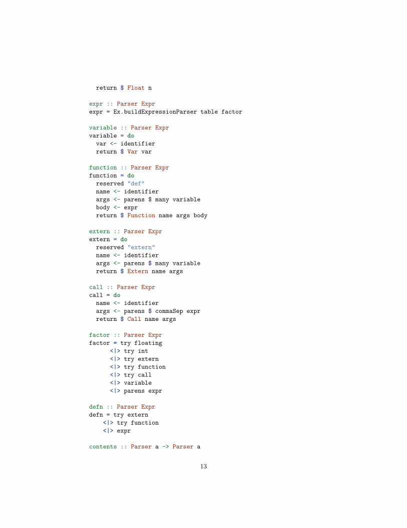
The AST for a program captures its behavior in such a way that it is easy forlater stages of the compiler (e.g. code generation) to interpret. We basicallywant one object for each construct in the language, and the AST should closelymodel the language. In Kaleidoscope, we have expressions, and a function object.When parsing with Parsec we will unpack tokens straight into our AST whichwe define as the Expr algebraic data type:

module Syntax where

type Name = String

data Expr= Float Double| BinOp Op Expr Expr| Var String

11

| Call Name [Expr]| Function Name [Expr] Expr| Extern Name [Expr]deriving (Eq, Ord, Show)

data Op= Plus| Minus| Times| Dividederiving (Eq, Ord, Show)

This is all (intentionally) rather straight-forward: variables capture the variablename, binary operators capture their operation (e.g. Plus, Minus, . . . ), andcalls capture a function name as well as a list of any argument expressions.

We create Parsec parser which will scan an input source and unpack it intoour Expr type. The code composes within the Parser to generate the resultingparser which is then executed using the parse function.

module Parser where

import Text.Parsecimport Text.Parsec.String (Parser)

import qualified Text.Parsec.Expr as Eximport qualified Text.Parsec.Token as Tok

import Lexerimport Syntax

binary s f assoc = Ex.Infix (reservedOp s >> return (BinOp f)) assoc

table = [[binary "*" Times Ex.AssocLeft,binary "/" Divide Ex.AssocLeft]

,[binary "+" Plus Ex.AssocLeft,binary "-" Minus Ex.AssocLeft]]

int :: Parser Exprint = do

n <- integerreturn $ Float (fromInteger n)

floating :: Parser Exprfloating = do

n <- float

12

return $ Float n

expr :: Parser Exprexpr = Ex.buildExpressionParser table factor

variable :: Parser Exprvariable = do

var <- identifierreturn $ Var var

function :: Parser Exprfunction = do

reserved "def"name <- identifierargs <- parens $ many variablebody <- exprreturn $ Function name args body

extern :: Parser Exprextern = do

reserved "extern"name <- identifierargs <- parens $ many variablereturn $ Extern name args

call :: Parser Exprcall = do

name <- identifierargs <- parens $ commaSep exprreturn $ Call name args

factor :: Parser Exprfactor = try floating

<|> try int<|> try extern<|> try function<|> try call<|> variable<|> parens expr

defn :: Parser Exprdefn = try extern

<|> try function<|> expr

contents :: Parser a -> Parser a

13

contents p = doTok.whiteSpace lexerr <- peofreturn r

toplevel :: Parser [Expr]toplevel = many $ do

def <- defnreservedOp ";"return def

parseExpr :: String -> Either ParseError ExprparseExpr s = parse (contents expr) "<stdin>" s

parseToplevel :: String -> Either ParseError [Expr]parseToplevel s = parse (contents toplevel) "<stdin>" s

The REPL

The driver for this simply invokes all of the compiler in a loop feeding theresulting artifacts to the next iteration. We will use the haskeline library to giveus readline interactions for the small REPL.

module Main where

import Parser

import Control.Monad.Transimport System.Console.Haskeline

process :: String -> IO ()process line = do

let res = parseToplevel linecase res of

Left err -> print errRight ex -> mapM_ print ex

main :: IO ()main = runInputT defaultSettings loop

whereloop = do

minput <- getInputLine "ready> "case minput of

14

Nothing -> outputStrLn "Goodbye."Just input -> (liftIO $ process input) >> loop

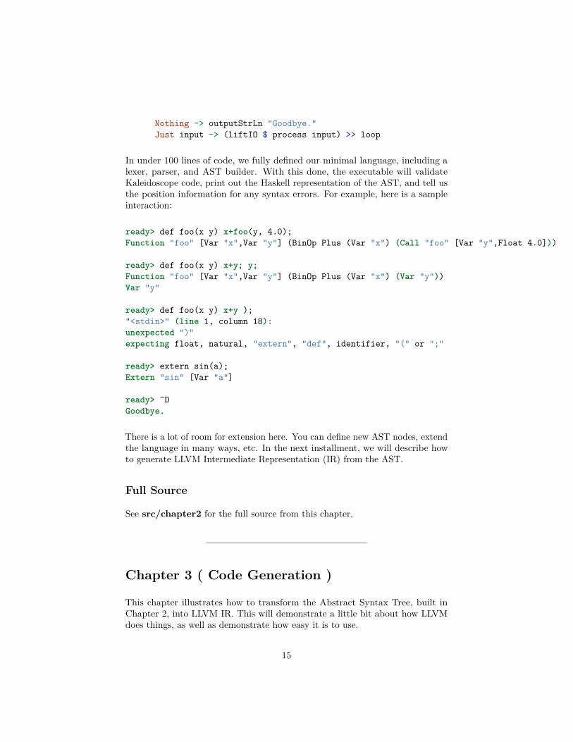
In under 100 lines of code, we fully defined our minimal language, including alexer, parser, and AST builder. With this done, the executable will validateKaleidoscope code, print out the Haskell representation of the AST, and tell usthe position information for any syntax errors. For example, here is a sampleinteraction:

ready> def foo(x y) x+foo(y, 4.0);Function "foo" [Var "x",Var "y"] (BinOp Plus (Var "x") (Call "foo" [Var "y",Float 4.0]))

ready> def foo(x y) x+y; y;Function "foo" [Var "x",Var "y"] (BinOp Plus (Var "x") (Var "y"))Var "y"

ready> def foo(x y) x+y );"<stdin>" (line 1, column 18):unexpected ")"expecting float, natural, "extern", "def", identifier, "(" or ";"

ready> extern sin(a);Extern "sin" [Var "a"]

ready> ^DGoodbye.

There is a lot of room for extension here. You can define new AST nodes, extendthe language in many ways, etc. In the next installment, we will describe howto generate LLVM Intermediate Representation (IR) from the AST.

Full Source

See src/chapter2 for the full source from this chapter.

Chapter 3 ( Code Generation )

This chapter illustrates how to transform the Abstract Syntax Tree, built inChapter 2, into LLVM IR. This will demonstrate a little bit about how LLVMdoes things, as well as demonstrate how easy it is to use.

15

Haskell LLVM Bindings

The LLVM bindings for Haskell are split across two packages:

• llvm-hs-pure is a pure Haskell representation of the LLVM IR.

• llvm-hs is the FFI bindings to LLVM required for constructing the C rep-resentation of the LLVM IR and performing optimization and compilation.

llvm-hs-pure does not require the LLVM libraries be available on the system.

On Hackage there is an older version of the LLVM bindings named llvm andllvm-base which should likely be avoided since they have not been updatedsince their development a few years ago.

As an aside, the GHCi can have issues with the FFI and can lead to errors whenworking with llvm-hs. If you end up with errors like the following, then youare likely trying to use GHCi or runhaskell and it is unable to link against yourLLVM library. Instead compile with standalone ghc.

Loading package llvm-hs-4.0.1.0... linking... ghc: /usr/lib/llvm-4.0/lib/libLLVMSupport.a: unknown symbol `_ZTVN4llvm14error_categoryE'ghc: unable to load package `llvm-hs-4.0.1.0'

Code Generation Setup

We start with a new Haskell module Codegen.hs which will hold the pure codegeneration logic that we’ll use to drive building the llvm-hs AST. For simplicity’ssake we’ll insist that all variables be of a single type, the double type.

double :: Typedouble = FloatingPointType 64 IEEE

To start we create a new record type to hold the internal state of our codegenerator as we walk the AST. We’ll use two records, one for the toplevel modulecode generation and one for basic blocks inside of function definitions.

type SymbolTable = [(String, Operand)]

data CodegenState= CodegenState {

currentBlock :: Name -- Name of the active block to append to, blocks :: Map.Map Name BlockState -- Blocks for function, symtab :: SymbolTable -- Function scope symbol table

16

, blockCount :: Int -- Count of basic blocks, count :: Word -- Count of unnamed instructions, names :: Names -- Name Supply} deriving Show

data BlockState= BlockState {

idx :: Int -- Block index, stack :: [Named Instruction] -- Stack of instructions, term :: Maybe (Named Terminator) -- Block terminator} deriving Show

We’ll hold the state of the code generator inside of Codegen State monad, theCodegen monad contains a map of block names to their BlockState representa-tion.

newtype Codegen a = Codegen { runCodegen :: State CodegenState a }deriving (Functor, Applicative, Monad, MonadState CodegenState )

At the top level we’ll create a LLVM State monad which will hold all codea for the LLVM module and upon evaluation will emit an llvm-hs Modulecontaining the AST. We’ll append to the list of definitions in the AST.Modulefield moduleDefinitions.

newtype LLVM a = LLVM (State AST.Module a)deriving (Functor, Applicative, Monad, MonadState AST.Module )

runLLVM :: AST.Module -> LLVM a -> AST.ModulerunLLVM mod (LLVM m) = execState m mod

emptyModule :: String -> AST.ModuleemptyModule label = defaultModule { moduleName = label }

addDefn :: Definition -> LLVM ()addDefn d = do

defs <- gets moduleDefinitionsmodify $ \s -> s { moduleDefinitions = defs ++ [d] }

Inside of our module we’ll need to insert our toplevel definitions. For our purposesthis will consist entirely of local functions and external function declarations.

define :: Type -> String -> [(Type, Name)] -> [BasicBlock] -> LLVM ()define retty label argtys body = addDefn $

GlobalDefinition $ functionDefaults {

17

name = Name label, parameters = ([Parameter ty nm [] | (ty, nm) <- argtys], False), returnType = retty, basicBlocks = body}

external :: Type -> String -> [(Type, Name)] -> LLVM ()external retty label argtys = addDefn $

GlobalDefinition $ functionDefaults {name = Name label

, linkage = L.External, parameters = ([Parameter ty nm [] | (ty, nm) <- argtys], False), returnType = retty, basicBlocks = []}

Blocks

With our monad we’ll create several functions to manipulate the current blockstate so that we can push and pop the block “cursor” and append instructionsinto the current block.

entry :: Codegen Nameentry = gets currentBlock

addBlock :: String -> Codegen NameaddBlock bname = do

bls <- gets blocksix <- gets blockCountnms <- gets names

let new = emptyBlock ix(qname, supply) = uniqueName bname nms

modify $ \s -> s { blocks = Map.insert (Name qname) new bls, blockCount = ix + 1, names = supply}

return (Name qname)

setBlock :: Name -> Codegen NamesetBlock bname = do

modify $ \s -> s { currentBlock = bname }return bname

18

getBlock :: Codegen NamegetBlock = gets currentBlock

modifyBlock :: BlockState -> Codegen ()modifyBlock new = do

active <- gets currentBlockmodify $ \s -> s { blocks = Map.insert active new (blocks s) }

current :: Codegen BlockStatecurrent = do

c <- gets currentBlockblks <- gets blockscase Map.lookup c blks of

Just x -> return xNothing -> error $ "No such block: " ++ show c

Instructions

Now that we have the basic infrastructure in place we’ll wrap the raw llvm-hsAST nodes inside a collection of helper functions to push instructions onto thestack held within our monad.

Instructions in LLVM are either numbered sequentially (%0, %1, . . . ) or givenexplicit variable names (%a, %foo, ..). For example, the arguments to thefollowing function are named values, while the result of the add instruction isunnamed.

define i32 @add(i32 %a, i32 %b) {%1 = add i32 %a, %bret i32 %1

}

In the implementation of llvm-hs both these types are represented in a sum typecontaining the constructors UnName and Name. For most of our purpose we willsimply use numbered expressions and map the numbers to identifiers within oursymbol table. Every instruction added will increment the internal counter, toaccomplish this we add a fresh name supply.

fresh :: Codegen Wordfresh = do

i <- gets countmodify $ \s -> s { count = 1 + i }return $ i + 1

19

Throughout our code we will however refer named values within the module,these have a special data type Name (with an associated IsString instance sothat Haskell can automatically perform the boilerplate coercions between Stringtypes) for which we’ll create a second name supply map which guarantees thatour block names are unique.

type Names = Map.Map String Int

uniqueName :: String -> Names -> (String, Names)uniqueName nm ns =

case Map.lookup nm ns ofNothing -> (nm, Map.insert nm 1 ns)Just ix -> (nm ++ show ix, Map.insert nm (ix+1) ns)

Since we can now work with named LLVM values we need to create severalfunctions for referring to references of values.

local :: Name -> Operandlocal = LocalReference double

externf :: Name -> Operandexternf = ConstantOperand . C.GlobalReference double

Our function externf will emit a named value which refers to a toplevel function(@add) in our module or will refer to an externally declared function (@putchar).For instance:

declare i32 @putchar(i32)

define i32 @add(i32 %a, i32 %b) {%1 = add i32 %a, %bret i32 %1

}

define void @main() {%1 = call i32 @add(i32 0, i32 97)call i32 @putchar(i32 %1)ret void

}

Since we’d like to refer to values on the stack by named quantities we’ll implementa simple symbol table as an association list letting us assign variable names tooperand quantities and subsequently look them up when used.

20

assign :: String -> Operand -> Codegen ()assign var x = do

lcls <- gets symtabmodify $ \s -> s { symtab = [(var, x)] ++ lcls }

getvar :: String -> Codegen Operandgetvar var = do

syms <- gets symtabcase lookup var syms of

Just x -> return xNothing -> error $ "Local variable not in scope: " ++ show var

Now that we have a way of naming instructions we’ll create an internal functionto take an llvm-hs AST node and push it on the current basic block stack. We’llreturn the left hand side reference of the instruction. Instructions will comein two flavors, instructions and terminators. Every basic block has a uniqueterminator and every last basic block in a function must terminate in a ret.

instr :: Instruction -> Codegen (Operand)instr ins = do

n <- freshlet ref = (UnName n)blk <- currentlet i = stack blkmodifyBlock (blk { stack = (ref := ins) : i } )return $ local ref

terminator :: Named Terminator -> Codegen (Named Terminator)terminator trm = do

blk <- currentmodifyBlock (blk { term = Just trm })return trm

Using the instr function we now wrap the AST nodes for basic arithmeticoperations of floating point values.

fadd :: Operand -> Operand -> Codegen Operandfadd a b = instr $ FAdd NoFastMathFlags a b []

fsub :: Operand -> Operand -> Codegen Operandfsub a b = instr $ FSub NoFastMathFlags a b []

fmul :: Operand -> Operand -> Codegen Operandfmul a b = instr $ FMul NoFastMathFlags a b []

21

fdiv :: Operand -> Operand -> Codegen Operandfdiv a b = instr $ FDiv NoFastMathFlags a b []

On top of the basic arithmetic functions we’ll add the basic control flow operationswhich will allow us to direct the control flow between basic blocks and returnvalues.

br :: Name -> Codegen (Named Terminator)br val = terminator $ Do $ Br val []

cbr :: Operand -> Name -> Name -> Codegen (Named Terminator)cbr cond tr fl = terminator $ Do $ CondBr cond tr fl []

ret :: Operand -> Codegen (Named Terminator)ret val = terminator $ Do $ Ret (Just val) []

Finally we’ll add several “effect” instructions which will invoke memory andevaluation side-effects. The call instruction will simply take a named functionreference and a list of arguments and evaluate it and simply invoke it at thecurrent position. The alloca instruction will create a pointer to a stack allocateduninitialized value of the given type.

call :: Operand -> [Operand] -> Codegen Operandcall fn args = instr $ Call Nothing CC.C [] (Right fn) (toArgs args) [] []

alloca :: Type -> Codegen Operandalloca ty = instr $ Alloca ty Nothing 0 []

store :: Operand -> Operand -> Codegen Operandstore ptr val = instr $ Store False ptr val Nothing 0 []

load :: Operand -> Codegen Operandload ptr = instr $ Load False ptr Nothing 0 []

From AST to IR

Now that we have the infrastructure in place we can begin ingest our AST fromSyntax.hs and construct a LLVM module from it. We will create a new Emit.hsmodule and spread the logic across two functions. The first codegenTop willemit toplevel constructions in modules ( functions and external definitions ) andwill return a LLVM monad. The last instruction on the stack we’ll bind into theret instruction to ensure and emit as the return value of the function. We’llalso sequentially assign each of the named arguments from the function to astack allocated value with a reference in our symbol table.

22

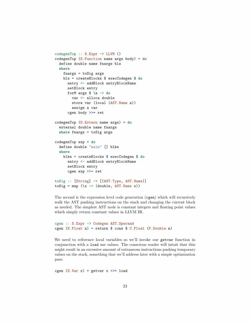
codegenTop :: S.Expr -> LLVM ()codegenTop (S.Function name args body) = do

define double name fnargs blswhere

fnargs = toSig argsbls = createBlocks $ execCodegen $ do

entry <- addBlock entryBlockNamesetBlock entryforM args $ \a -> do

var <- alloca doublestore var (local (AST.Name a))assign a var

cgen body >>= ret

codegenTop (S.Extern name args) = doexternal double name fnargswhere fnargs = toSig args

codegenTop exp = dodefine double "main" [] blkswhere

blks = createBlocks $ execCodegen $ doentry <- addBlock entryBlockNamesetBlock entrycgen exp >>= ret

toSig :: [String] -> [(AST.Type, AST.Name)]toSig = map (\x -> (double, AST.Name x))

The second is the expression level code generation (cgen) which will recursivelywalk the AST pushing instructions on the stack and changing the current blockas needed. The simplest AST node is constant integers and floating point valueswhich simply return constant values in LLVM IR.

cgen :: S.Expr -> Codegen AST.Operandcgen (S.Float n) = return $ cons $ C.Float (F.Double n)

We need to reference local variables so we’ll invoke our getvar function inconjunction with a load use values. The conscious reader will intuit that thismight result in an excessive amount of extraneous instructions pushing temporaryvalues on the stack, something that we’ll address later with a simple optimizationpass.

cgen (S.Var x) = getvar x >>= load

23

For Call we’ll first evaluate each argument and then invoke the function withthe values. Since our language only has double type values, this is trivial andwe don’t need to worry too much.

cgen (S.Call fn args) = dolargs <- mapM cgen argscall (externf (AST.Name fn)) largs

Finally for our operators we’ll construct a predefined association map of symbolstrings to implementations of functions with the corresponding logic for theoperation.

binops = Map.fromList [("+", fadd)

, ("-", fsub), ("*", fmul), ("/", fdiv), ("<", lt)

]

For the comparison operator we’ll invoke the uitofp which will convert aunsigned integer quantity to a floating point value. LLVM requires the unsignedsingle bit types as the values for comparison and test operations but we preferto work entirely with doubles where possible.

lt :: AST.Operand -> AST.Operand -> Codegen AST.Operandlt a b = do

test <- fcmp FP.ULT a buitofp double test

Just like the call instruction above we simply generate the code for operandsand invoke the function we just looked up for the symbol.

cgen (S.BinaryOp op a b) = docase Map.lookup op binops of

Just f -> doca <- cgen acb <- cgen bf ca cb

Nothing -> error "No such operator"

Putting everything together we find that we nice little minimal language thatsupports both function abstraction and basic arithmetic. The final step is tohook into LLVM bindings to generate a string representation of the LLVM IRwhich will print out the string on each action in the REPL. We’ll discuss thesefunctions in more depth in the next chapter.

24

codegen :: AST.Module -> [S.Expr] -> IO AST.Modulecodegen mod fns = withContext $ \context ->

liftError $ withModuleFromAST context newast $ \m -> dollstr <- moduleLLVMAssembly mputStrLn llstrreturn newast

wheremodn = mapM codegenTop fnsnewast = runLLVM mod modn

Running Main.hs we can observe our code generator in action.

ready> def foo(a b) a*a + 2*a*b + b*b;; ModuleID = 'my cool jit'

define double @foo(double %a, double %b) {entry:

%0 = fmul double %a, %a%1 = fmul double %a, 2.000000e+00%2 = fmul double %1, %b%3 = fadd double %0, %2%4 = fmul double %b, %b%5 = fadd double %4, %3ret double %5

}

ready> def bar(a) foo(a, 4.0) + bar(31337);define double @bar(double %a) {entry:

%0 = alloca doublestore double %a, double* %0%1 = load double* %0%2 = call double @foo(double %1, double 4.000000e+00)%3 = call double @bar(double 3.133700e+04)%4 = fadd double %2, %3ret double %4

}

Full Source

See src/chapter3 for the full source from this chapter.

25

Chapter 4 ( JIT and Optimizer Support )

In the previous chapter we were able to map our language Syntax into theLLVM IR and print it out to the screen. This chapter describes two newtechniques: adding optimizer support to our language, and adding JIT compilersupport. These additions will demonstrate how to get nice, efficient code for theKaleidoscope language.

ASTs and Modules

We’ll refer to a Module as holding the internal representation of the LLVMIR. Modules can be generated from the Haskell LLVM AST or from stringscontaining bitcode.

Both data types have the same name ( Module ), so as convention we will qualifythe imports of the libraries to distinguish between the two.

• AST.Module : Haskell AST Module• Module : Internal LLVM Module

llvm-hs provides two important functions for converting between them.withModuleFromAST has type ExceptT since it may fail if given a malformedexpression, it is important to handle both cases of the resulting Either value.

withModuleFromAST :: Context -> AST.Module -> (Module -> IO a) -> ExceptT String IO amoduleAST :: Module -> IO AST.Module

We can also generate the assembly code for our given module by passing aspecification of the CPU and platform information we wish to target, called theTargetMachine.

moduleTargetAssembly :: TargetMachine -> Module -> ExceptT String IO String

Recall the so called “Bracket” pattern in Haskell for managing IO resources.llvm-hs makes heavy use this pattern to manage the life-cycle of certain LLVMresources. It is very important to remember not to pass or attempt to useresources outside of the bracket as this will lead to undefined behavior and/orsegfaults.

bracket :: IO a -- computation to run first ("acquire resource")-> (a -> IO b) -- computation to run last ("release resource")-> (a -> IO c) -- computation to run in-between-> IO c

26

In addition to this we’ll often be dealing with operations which can fail in anEitherT monad if given bad code. We’ll often want to lift this error up themonad transformer stack with the pattern:

liftExcept :: ExceptT String IO a -> IO aliftExcept = runExceptT >=> either fail return

To start we’ll create a runJIT function which will start with a stack of brackets.We’ll then simply generate the IR and print it out to the screen.

runJIT :: AST.Module -> IO (Either String ())runJIT mod = do

withContext $ \context ->runErrorT $ withModuleFromAST context mod $ \m ->

s <- moduleLLVMAssembly mputStrLn s

Constant Folding

Our demonstration for Chapter 3 is elegant and easy to extend. Unfortunately, itdoes not produce wonderful code. However the naive construction of the LLVMmodule will perform some minimal transformations to generate a module whichnot a literal transcription of the AST but preserves the same semantics.

The “dumb” transcription would look like:

ready> def test(x) 1+2+x;define double @test(double %x) {entry:

%addtmp = fadd double 2.000000e+00, 1.000000e+00%addtmp1 = fadd double %addtmp, %xret double %addtmp1

}

The “smarter” transcription would eliminate the first line since it contains asimple constant that can be computed at compile-time.

ready> def test(x) 1+2+x;define double @test(double %x) {entry:

%addtmp = fadd double 3.000000e+00, %xret double %addtmp

}

27

Constant folding, as seen above, in particular, is a very common and veryimportant optimization: so much so that many language implementors implementconstant folding support in their AST representation. This technique is limitedby the fact that it does all of its analysis inline with the code as it is built. Ifyou take a slightly more complex example:

ready> def test(x) (1+2+x)*(x+(1+2));define double @test(double %x) {entry:

%addtmp = fadd double 3.000000e+00, %x%addtmp1 = fadd double %x, 3.000000e+00%multmp = fmul double %addtmp, %addtmp1ret double %multmp

}

In this case, the left and right hand sides of the multiplication are the same value.We’d really like to see this generate tmp = x+3; result = tmp*tmp instead ofcomputing x+3 twice.

Unfortunately, no amount of local analysis will be able to detect and correctthis. This requires two transformations: reassociation of expressions (to makethe adds lexically identical) and Common Subexpression Elimination (CSE) todelete the redundant add instruction. Fortunately, LLVM provides a broad rangeof optimizations that we can use, in the form of “passes”.

Optimization Passes

LLVM provides many optimization passes, which do many different sorts ofthings and have different trade-offs. Unlike other systems, LLVM doesn’t holdto the mistaken notion that one set of optimizations is right for all languagesand for all situations. LLVM allows a compiler implementor to make completedecisions about what optimizations to use, in which order, and in what situation.

As a concrete example, LLVM supports both “whole module” passes, which lookacross as large of body of code as they can (often a whole file, but if run at linktime, this can be a substantial portion of the whole program). It also supportsand includes “per-function” passes which just operate on a single function at atime, without looking at other functions. For more information on passes andhow they are run, see the How to Write a Pass document and the List of LLVMPasses.

For Kaleidoscope, we are currently generating functions on the fly, one at a time,as the user types them in. We aren’t shooting for the ultimate optimizationexperience in this setting, but we also want to catch the easy and quick stuffwhere possible.

28

We won’t delve too much into the details of the passes since they are betterdescribed elsewhere. We will instead just invoke the default “curated passes”with an optimization level which will perform most of the common clean-upsand a few non-trivial optimizations.

passes :: PassSetSpecpasses = defaultCuratedPassSetSpec { optLevel = Just 3 }

To apply the passes we create a bracket for a PassManager and invokerunPassManager on our working module. Note that this modifies the modulein-place.

runJIT :: AST.Module -> IO (Either String AST.Module)runJIT mod = do

withContext $ \context ->runExceptT $ withModuleFromAST context mod $ \m ->

withPassManager passes $ \pm -> dorunPassManager pm moptmod <- moduleAST ms <- moduleLLVMAssembly mputStrLn sreturn optmod

With this in place, we can try our test above again:

ready> def test(x) (1+2+x)*(x+(1+2));; ModuleID = 'my cool jit'

; Function Attrs: nounwind readnonedefine double @test(double %x) #0 {entry:

%0 = fadd double %x, 3.000000e+00%1 = fmul double %0, %0ret double %1

}

attributes #0 = { nounwind readnone }

As expected, we now get our nicely optimized code, saving a floating pointadd instruction from every execution of this function. We also see some extrametadata attached to our function, which we can ignore for now, but is indicatingcertain properties of the function that aid in later optimization.

LLVM provides a wide variety of optimizations that can be used in certaincircumstances. Some documentation about the various passes is available, but it

29

isn’t very complete. Another good source of ideas can come from looking at thepasses that Clang runs to get started. The “opt” tool allows us to experimentwith passes from the command line, so we can see if they do anything.

One important optimization pass is an “analysis pass” which will validate thatthe internal IR is well-formed. Since it quite possible (even easy!) to constructnonsensical or unsafe IR it is very good practice to validate our IR beforeattempting to optimize or execute it. To do so, we simply invoke the verifyfunction with our active module.

runJIT :: AST.Module -> IO (Either String AST.Module)runJIT mod = do

...

withPassManager passes $ \pm -> dorunExceptT $ verify m

Now that we have reasonable code coming out of our front-end, let’s talk aboutexecuting it!

Adding a JIT Compiler

Code that is available in LLVM IR can have a wide variety of tools applied to it.For example, we can run optimizations on it (as we did above), we can dump itout in textual or binary forms, we can compile the code to an assembly file (.s)for some target, or we can JIT compile it. The nice thing about the LLVM IRrepresentation is that it is the “common currency” between many different partsof the compiler.

In this section, we’ll add JIT compiler support to our interpreter. The basicidea that we want for Kaleidoscope is to have the user enter function bodies asthey do now, but immediately evaluate the top-level expressions they type in.For example, if they type in “1 + 2;”, we should evaluate and print out 3. Ifthey define a function, they should be able to call it from the command line.

In order to do this, we add another function to bracket the creation of the JITExecution Engine. There are two provided engines: jit and mcjit. The distinctionis not important for us but we will opt to use the newer mcjit.

import qualified LLVM.ExecutionEngine as EE

jit :: Context -> (EE.MCJIT -> IO a) -> IO ajit c = EE.withMCJIT c optlevel model ptrelim fastins

whereoptlevel = Just 2 -- optimization level

30

model = Nothing -- code model ( Default )ptrelim = Nothing -- frame pointer eliminationfastins = Nothing -- fast instruction selection

The result of the JIT compiling our function will be a C function pointer which wecan call from within the JIT’s process space. We need some (unsafe!) plumbingto coerce our foreign C function into a callable object from Haskell. Some caremust be taken when performing these operations since we’re telling Haskell to“trust us” that the pointer we hand it is actually typed as we describe it. If wedon’t take care with the casts we can expect undefined behavior.

foreign import ccall "dynamic" haskFun :: FunPtr (IO Double) -> (IO Double)

run :: FunPtr a -> IO Doublerun fn = haskFun (castFunPtr fn :: FunPtr (IO Double))

Integrating this with our function from above we can now manifest our IR asexecutable code inside the ExecutionEngine and pass the resulting native typesto and from the Haskell runtime.

runJIT :: AST.Module -> IO (Either String ())runJIT mod = do

...jit context $ \executionEngine ->

...EE.withModuleInEngine executionEngine m $ \ee -> do

mainfn <- EE.getFunction ee (AST.Name "main")case mainfn of

Just fn -> dores <- run fnputStrLn $ "Evaluated to: " ++ show res

Nothing -> return ()

Having to statically declare our function pointer type is rather inflexible. If wewish to extend to this to be more flexible, a library like libffi is very useful forcalling functions with argument types that can be determined at runtime.

External Functions

The JIT provides a number of other more advanced interfaces for things likefreeing allocated machine code, rejit’ing functions to update them, etc. However,even with this simple code, we get some surprisingly powerful capabilities - checkthis out:

31

ready> extern sin(x);; ModuleID = 'my cool jit'

declare double @sin(double)

ready> extern cos(x);; ModuleID = 'my cool jit'

declare double @sin(double)

declare double @cos(double)

ready> sin(1.0);; ModuleID = 'my cool jit'

declare double @sin(double)

declare double @cos(double)

define double @main() {entry:

%0 = call double @sin(double 1.000000e+00)ret double %0

}

Evaluated to: 0.8414709848078965

Whoa, how does the JIT know about sin and cos? The answer is surprisinglysimple: in this example, the JIT started execution of a function and got to afunction call. It realized that the function was not yet JIT compiled and invokedthe standard set of routines to resolve the function. In this case, there is nobody defined for the function, so the JIT ended up calling dlsym("sin") on theKaleidoscope process itself. Since “sin” is defined within the JIT’s address space,it simply patches up calls in the module to call the libm version of sin directly.

The LLVM JIT provides a number of interfaces for controlling how unknownfunctions get resolved. It allows us to establish explicit mappings between IRobjects and addresses (useful for LLVM global variables that we want to map tostatic tables, for example), allows us to dynamically decide on the fly based onthe function name, and even allows us JIT compile functions lazily the first timethey’re called.

One interesting application of this is that we can now extend the language bywriting arbitrary C code to implement operations. For example, we create ashared library cbits.so:

32

/* cbits$ gcc -fPIC -shared cbits.c -o cbits.so$ clang -fPIC -shared cbits.c -o cbits.so*/

#include "stdio.h"

// putchard - putchar that takes a double and returns 0.double putchard(double X) {

putchar((char)X);fflush(stdout);return 0;

}

Compile this with your favorite C compiler. We can then link this into ourHaskell binary by simply including it alongside the rest of the Haskell sourcefiles:

$ ghc cbits.so --make Main.hs -o Main

Now we can produce simple output to the console by using things like: externputchard(x); putchard(120);, which prints a lowercase ‘x’ on the console(120 is the ASCII code for ‘x’). Similar code could be used to implement fileI/O, console input, and many other capabilities in Kaleidoscope.

To bring external shared objects into the process address space we can callHaskell’s bindings to the system dynamic linking loader to load external libraries.In addition if we are statically compiling our interpreter we can tell GHC to linkagainst the shared objects explicitly by passing them in with the -l flag.

This completes the JIT and optimizer chapter of the Kaleidoscope tutorial.At this point, we can compile a non-Turing-complete programming language,optimize and JIT compile it in a user-driven way. Next up we’ll look intoextending the language with control flow constructs, tackling some interestingLLVM IR issues along the way.

Full Source

See src/chapter4 for the full source from this chapter.

33

Chapter 5 ( Control Flow )

Welcome to Chapter 5 of the Implementing a language with LLVM tutorial.Parts 1-4 described the implementation of the simple Kaleidoscope languageand included support for generating LLVM IR, followed by optimizations and aJIT compiler. Unfortunately, as presented, Kaleidoscope is mostly useless: ithas no control flow other than call and return. This means that we can’t haveconditional branches in the code, significantly limiting its power. In this episodeof “build that compiler”, we’ll extend Kaleidoscope to have an if/then/elseexpression plus a simple ‘for’ loop.

‘if’ Expressions

Extending Kaleidoscope to support if/then/else is quite straightforward. Itbasically requires adding lexer support for this “new” concept to the lexer,parser, AST, and LLVM code emitter. This example is nice, because it showshow easy it is to “grow” a language over time, incrementally extending it as newideas are discovered.

Before we get going on “how” we add this extension, let’s talk about “what” wewant. The basic idea is that we want to be able to write this sort of thing:

def fib(x)if x < 3 then

1else

fib(x-1) + fib(x-2);

In Kaleidoscope, every construct is an expression: there are no statements. Assuch, the if/then/else expression needs to return a value like any other. Sincewe’re using a mostly functional form, we’ll have it evaluate its conditional, thenreturn the ‘then’ or ‘else’ value based on how the condition was resolved. This isvery similar to the C “?:” expression.

The semantics of the if/then/else expression is that it evaluates the conditionto a boolean equality value: 0.0 is considered to be false and everything else isconsidered to be true. If the condition is true, the first subexpression is evaluatedand returned, if the condition is false, the second subexpression is evaluated andreturned. Since Kaleidoscope allows side-effects, this behavior is important tonail down.

Now that we know what we “want”, let’s break this down into its constituentpieces.

To represent the new expression we add a new AST node for it:

34

data Expr...| If Expr Expr Exprderiving (Eq, Ord, Show)

We also extend our lexer definition with the new reserved names.

lexer :: Tok.TokenParser ()lexer = Tok.makeTokenParser style

whereops = ["+","*","-","/",";",",","<"]names = ["def","extern","if","then","else"]style = emptyDef {

Tok.commentLine = "#", Tok.reservedOpNames = ops, Tok.reservedNames = names}

Now that we have the relevant tokens coming from the lexer and we have theAST node to build, our parsing logic is relatively straightforward. First we definea new parsing function:

ifthen :: Parser Exprifthen = do

reserved "if"cond <- exprreserved "then"tr <- exprreserved "else"fl <- exprreturn $ If cond tr fl

Now that we have it parsing and building the AST, the final piece is adding LLVMcode generation support. This is the most interesting part of the if/then/elseexample, because this is where it starts to introduce new concepts. All of thecode above has been thoroughly described in previous chapters.

To motivate the code we want to produce, let’s take a look at a simple example.Consider:

extern foo();extern bar();def baz(x) if x then foo() else bar();

35

declare double @foo()

declare double @bar()

define double @baz(double %x) {entry:

%ifcond = fcmp one double %x, 0.000000e+00br i1 %ifcond, label %then, label %else

then: ; preds = %entry%calltmp = call double @foo()br label %ifcont

else: ; preds = %entry%calltmp1 = call double @bar()br label %ifcont

ifcont: ; preds = %else, %then%iftmp = phi double [ %calltmp, %then ], [ %calltmp1, %else ]ret double %iftmp

}

To visualize the control flow graph, we can use a nifty feature of the LLVM opttool. If we put this LLVM IR into “t.ll” and run

$ llvm-as < t.ll | opt -analyze -view-cfg

A window will pop up and we’ll see this graph:

LLVM has many nice features for visualizing various graphs, but note that theseare available only if your LLVM was built with Graphviz support (accomplishedby having Graphviz and Ghostview installed when building LLVM).

Getting back to the generated code, it is fairly simple: the entry block evaluatesthe conditional expression (“x” in our case here) and compares the result to 0.0with the fcmp one instruction (one is “Ordered and Not Equal”). Based on theresult of this expression, the code jumps to either the “then” or “else” blocks,which contain the expressions for the true/false cases.

Once the then/else blocks are finished executing, they both branch back to theif.exit block to execute the code that happens after the if/then/else. In thiscase the only thing left to do is to return to the caller of the function. Thequestion then becomes: how does the code know which expression to return?

The answer to this question involves an important SSA operation: the Phioperation. If you’re not familiar with SSA, the Wikipedia article is a goodintroduction and there are various other introductions to it available on your

36

Figure 2:

favorite search engine. The short version is that “execution” of the Phi operationrequires “remembering” which block control came from. The Phi operation takeson the value corresponding to the input control block. In this case, if controlcomes in from the if.then block, it gets the value of calltmp. If control comesfrom the if.else block, it gets the value of calltmp1.

At this point, you are probably starting to think “Oh no! This means mysimple and elegant front-end will have to start generating SSA form in orderto use LLVM!”. Fortunately, this is not the case, and we strongly advise notimplementing an SSA construction algorithm in your front-end unless there is anamazingly good reason to do so. In practice, there are two sorts of values thatfloat around in code written for your average imperative programming languagethat might need Phi nodes:

• Code that involves user variables: x = 1; x = x + 1;• Values that are implicit in the structure of your AST, such as the Phi node

in this case.

In Chapter 7 of this tutorial (“mutable variables”), we’ll talk about #1 in depth.For now, just believe and accept that you don’t need SSA construction to handlethis case. For #2, you have the choice of using the techniques that we willdescribe for #1, or you can insert Phi nodes directly, if convenient. In this case,it is really really easy to generate the Phi node, so we choose to do it directly.

37

Okay, enough of the motivation and overview, let’s generate code!

In order to generate code for this, we implement the Codegen method for Ifnode:

cgen (S.If cond tr fl) = doifthen <- addBlock "if.then"ifelse <- addBlock "if.else"ifexit <- addBlock "if.exit"

-- %entry------------------cond <- cgen condtest <- fcmp FP.ONE false condcbr test ifthen ifelse -- Branch based on the condition

-- if.then------------------setBlock ifthentrval <- cgen tr -- Generate code for the true branchbr ifexit -- Branch to the merge blockifthen <- getBlock

-- if.else------------------setBlock ifelseflval <- cgen fl -- Generate code for the false branchbr ifexit -- Branch to the merge blockifelse <- getBlock

-- if.exit------------------setBlock ifexitphi double [(trval, ifthen), (flval, ifelse)]

We start by creating three blocks.

ifthen <- addBlock "if.then"ifelse <- addBlock "if.else"ifexit <- addBlock "if.exit"

Next emit the expression for the condition, then compare that value to zero toget a truth value as a 1-bit (i.e. bool) value. We end this entry block by emittingthe conditional branch that chooses between the two cases.

38

test <- fcmp FP.ONE false condcbr test ifthen ifelse -- Branch based on the condition

After the conditional branch is inserted, we move switch blocks to start insertinginto the if.then block.

setBlock ifthen

We recursively codegen the tr expression from the AST. To finish off the if.thenblock, we create an unconditional branch to the merge block. One interesting(and very important) aspect of the LLVM IR is that it requires all basic blocks tobe “terminated” with a control flow instruction such as return or branch. Thismeans that all control flow, including fallthroughs must be made explicit in theLLVM IR. If we violate this rule, the verifier will emit an error.

trval <- cgen tr -- Generate code for the true branchbr ifexit -- Branch to the merge blockifthen <- getBlock -- Get the current block

The final line here is quite subtle, but is very important. The basic issue isthat when we create the Phi node in the merge block, we need to set up theblock/value pairs that indicate how the Phi will work. Importantly, the Phi nodeexpects to have an entry for each predecessor of the block in the CFG. Whythen, are we getting the current block when we just set it 3 lines above? Theproblem is that theifthen expression may actually itself change the block thatthe Builder is emitting into if, for example, it contains a nested “if/then/else”expression. Because calling cgen recursively could arbitrarily change the notionof the current block, we are required to get an up-to-date value for code thatwill set up the Phi node.

setBlock ifelseflval <- cgen fl -- Generate code for the false branchbr ifexit -- Branch to the merge blockifelse <- getBlock

Code generation for the if.else block is basically identical to codegen for theif.then block.

setBlock ifexitphi double [(trval, ifthen), (flval, ifelse)]

The first line changes the insertion point so that newly created code will go intothe if.exit block. Once that is done, we need to create the Phi node and setup the block/value pairs for the Phi.

39

Finally, the cgen function returns the phi node as the value computed by theif/then/else expression. In our example above, this returned value will feed intothe code for the top-level function, which will create the return instruction.

Overall, we now have the ability to execute conditional code in Kaleidoscope.With this extension, Kaleidoscope is a fairly complete language that can calculatea wide variety of numeric functions. Next up we’ll add another useful expressionthat is familiar from non-functional languages. . .

‘for’ Loop Expressions

Now that we know how to add basic control flow constructs to the language, wehave the tools to add more powerful things. Let’s add something more aggressive,a ‘for’ expression:

extern putchard(char);

def printstar(n)for i = 1, i < n, 1.0 in

putchard(42); # ascii 42 = '*'

# print 100 '*' charactersprintstar(100);

This expression defines a new variable (i in this case) which iterates from astarting value, while the condition (i < n in this case) is true, incrementing byan optional step value (1.0 in this case). While the loop is true, it executes itsbody expression. Because we don’t have anything better to return, we’ll justdefine the loop as always returning 0.0. In the future when we have mutablevariables, it will get more useful.

To get started, we again extend our lexer with new reserved names “for” and“in”.

lexer :: Tok.TokenParser ()lexer = Tok.makeTokenParser style

whereops = ["+","*","-","/",";",",","<"]names = ["def","extern","if","then","else","in","for"]style = emptyDef {

Tok.commentLine = "#", Tok.reservedOpNames = ops, Tok.reservedNames = names}

40

As before, let’s talk about the changes that we need to Kaleidoscope to supportthis. The AST node is just as simple. It basically boils down to capturing thevariable name and the constituent expressions in the node.

data Expr...| For Name Expr Expr Expr Exprderiving (Eq, Ord, Show)

The parser code captures a named value for the iterator variable and the fourexpressions objects for the parameters of the loop parameters.

for :: Parser Exprfor = do

reserved "for"var <- identifierreservedOp "="start <- exprreservedOp ","cond <- exprreservedOp ","step <- exprreserved "in"body <- exprreturn $ For var start cond step body

Now we get to the good part: the LLVM IR we want to generate for this thing.With the simple example above, we get this LLVM IR (note that this dump isgenerated with optimizations disabled for clarity):

declare double @putchard(double)

define double @printstar(double %n) {entry:

br label %loop

loop:%i = phi double [ 1.000000e+00, %entry ], [ %nextvar, %loop ]%calltmp = call double @putchard(double 4.200000e+01)%nextvar = fadd double %i, 1.000000e+00

%cmptmp = fcmp ult double %i, %n%booltmp = uitofp i1 %cmptmp to double%loopcond = fcmp one double %booltmp, 0.000000e+00

41

br i1 %loopcond, label %loop, label %afterloop

afterloop:ret double 0.000000e+00

}

Figure 3:

The code to generate this is only slightly more complicated than the above “if”statement.

cgen (S.For ivar start cond step body) = doforloop <- addBlock "for.loop"forexit <- addBlock "for.exit"

-- %entry------------------i <- alloca doubleistart <- cgen start -- Generate loop variable initial valuestepval <- cgen step -- Generate loop variable step

42

store i istart -- Store the loop variable initial valueassign ivar i -- Assign loop variable to the variable namebr forloop -- Branch to the loop body block

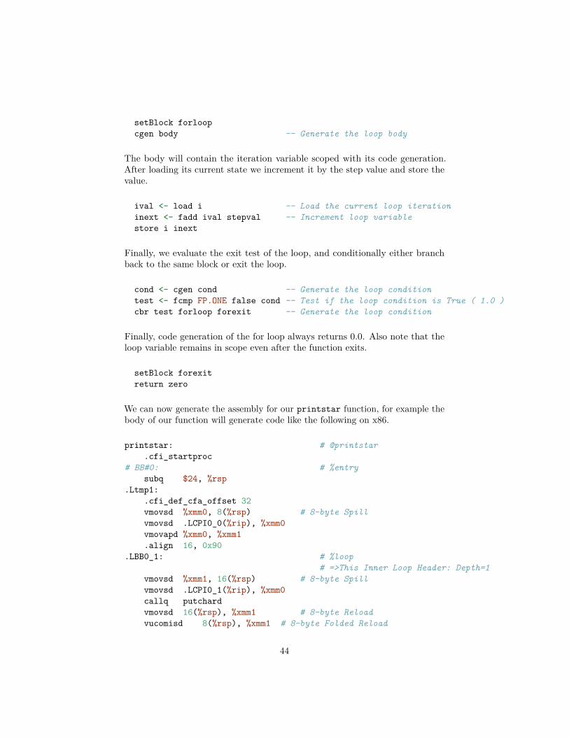
-- for.loop------------------setBlock forloopcgen body -- Generate the loop bodyival <- load i -- Load the current loop iterationinext <- fadd ival stepval -- Increment loop variablestore i inext

cond <- cgen cond -- Generate the loop conditiontest <- fcmp FP.ONE false cond -- Test if the loop condition is True ( 1.0 )cbr test forloop forexit -- Generate the loop condition

The first step is to set up the LLVM basic block for the start of the loop body.In the case above, the whole loop body is one block, but remember that thegenerating code for the body of the loop could consist of multiple blocks (e.g. ifit contains an if/then/else or a for/in expression).

forloop <- addBlock "for.loop"forexit <- addBlock "for.exit"

Next we allocate the iteration variable and generate the code for the constantinitial value and step.

i <- alloca doubleistart <- cgen start -- Generate loop variable initial valuestepval <- cgen step -- Generate loop variable step

Now the code starts to get more interesting. Our ‘for’ loop introduces a newvariable to the symbol table. This means that our symbol table can now containeither function arguments or loop variables. Once the loop variable is set intothe symbol table, the code recursively codegen’s the body. This allows the bodyto use the loop variable: any references to it will naturally find it in the symboltable.

store i istart -- Store the loop variable initial valueassign ivar i -- Assign loop variable to the variable namebr forloop -- Branch to the loop body block

Now that the “preheader” for the loop is set up, we switch to emitting code forthe loop body.

43

setBlock forloopcgen body -- Generate the loop body

The body will contain the iteration variable scoped with its code generation.After loading its current state we increment it by the step value and store thevalue.

ival <- load i -- Load the current loop iterationinext <- fadd ival stepval -- Increment loop variablestore i inext

Finally, we evaluate the exit test of the loop, and conditionally either branchback to the same block or exit the loop.

cond <- cgen cond -- Generate the loop conditiontest <- fcmp FP.ONE false cond -- Test if the loop condition is True ( 1.0 )cbr test forloop forexit -- Generate the loop condition

Finally, code generation of the for loop always returns 0.0. Also note that theloop variable remains in scope even after the function exits.

setBlock forexitreturn zero

We can now generate the assembly for our printstar function, for example thebody of our function will generate code like the following on x86.

printstar: # @printstar.cfi_startproc

# BB#0: # %entrysubq $24, %rsp

.Ltmp1:.cfi_def_cfa_offset 32vmovsd %xmm0, 8(%rsp) # 8-byte Spillvmovsd .LCPI0_0(%rip), %xmm0vmovapd %xmm0, %xmm1.align 16, 0x90

.LBB0_1: # %loop# =>This Inner Loop Header: Depth=1

vmovsd %xmm1, 16(%rsp) # 8-byte Spillvmovsd .LCPI0_1(%rip), %xmm0callq putchardvmovsd 16(%rsp), %xmm1 # 8-byte Reloadvucomisd 8(%rsp), %xmm1 # 8-byte Folded Reload

44

sbbl %eax, %eaxandl $1, %eaxvcvtsi2sd %eax, %xmm0, %xmm0vaddsd .LCPI0_0(%rip), %xmm1, %xmm1vucomisd .LCPI0_2, %xmm0jne .LBB0_1

# BB#2: # %afterloopvxorpd %xmm0, %xmm0, %xmm0addq $24, %rspret

Full Source

See src/chapter5 for the full source from this chapter.

Chapter 6 ( Operators )

Welcome to Chapter 6 of the “Implementing a language with LLVM” tutorial.At this point in our tutorial, we now have a fully functional language that isfairly minimal, but also useful. There is still one big problem with it, however.Our language doesn’t have many useful operators (like division, logical negation,or even any comparisons besides less-than).

This chapter of the tutorial takes a wild digression into adding user-definedoperators to the simple and beautiful Kaleidoscope language. This digressionnow gives us a simple and ugly language in some ways, but also a powerful oneat the same time. One of the great things about creating our own language isthat we get to decide what is good or bad. In this tutorial we’ll assume that itis okay to use this as a way to show some interesting parsing techniques.

At the end of this tutorial, we’ll run through an example Kaleidoscope applicationthat renders the Mandelbrot set. This gives an example of what we can buildwith Kaleidoscope and its feature set.

User-defined Operators

The “operator overloading” that we will add to Kaleidoscope is more general thanlanguages like C++. In C++, we are only allowed to redefine existing operators:we can’t programmatically change the grammar, introduce new operators, changeprecedence levels, etc. In this chapter, we will add this capability to Kaleidoscope,which will let the user round out the set of operators that are supported.

45

The two specific features we’ll add are programmable unary operators (rightnow, Kaleidoscope has no unary operators at all) as well as binary operators.An example of this is:

# Logical unary not.def unary!(v)

if v then0

else1;

# Define > with the same precedence as <.def binary> 10 (LHS RHS)

RHS < LHS;

# Binary "logical or", (note that it does not "short circuit")def binary| 5 (LHS RHS)

if LHS then1

else if RHS then1

else0;

# Define = with slightly lower precedence than relationals.def binary= 9 (LHS RHS)

!(LHS < RHS | LHS > RHS);

Many languages aspire to being able to implement their standard runtime libraryin the language itself. In Kaleidoscope, we can implement significant parts ofthe language in the library!

We will break down implementation of these features into two parts: implement-ing support for user-defined binary operators and adding unary operators.

Binary Operators

We extend the lexer with two new keywords for “binary” and “unary” topleveldefinitions.

lexer :: Tok.TokenParser ()lexer = Tok.makeTokenParser style

whereops = ["+","*","-","/",";","=",",","<",">","|",":"]names = ["def","extern","if","then","else","in","for"

46

,"binary", "unary"]style = emptyDef {

Tok.commentLine = "#", Tok.reservedOpNames = ops, Tok.reservedNames = names}

Parsec has no default function to parse “any symbolic” string, but it can beadded simply by defining an operator new token.

operator :: Parser Stringoperator = do

c <- Tok.opStart emptyDefcs <- many $ Tok.opLetter emptyDefreturn (c:cs)

Using this we can then parse any binary expression. By default all our operatorswill be left-associative and have equal precedence, except for the bulletins weprovide. A more general system would allow the parser to have internal stateabout the known precedences of operators before parsing. Without predefinedprecedence values we’ll need to disambiguate expressions with parentheses.

binop = Ex.Infix (BinaryOp <$> op) Ex.AssocLeft

Using the expression parser we can extend our table of operators with the “binop”class of custom operators. Note that this will match any and all operators evenat parse-time, even if there is no corresponding definition.

binops = [[binary "*" Ex.AssocLeft,binary "/" Ex.AssocLeft]

,[binary "+" Ex.AssocLeft,binary "-" Ex.AssocLeft]

,[binary "<" Ex.AssocLeft]]

expr :: Parser Exprexpr = Ex.buildExpressionParser (binops ++ [[binop]]) factor

The extensions to the AST consist of adding new toplevel declarations for theoperator definitions.

data Expr =...| BinaryOp Name Expr Expr| UnaryOp Name Expr| BinaryDef Name [Name] Expr| UnaryDef Name [Name] Expr

47

The parser extension is straightforward and essentially a function definition witha few slight changes. Note that we capture the string value of the operator asgiven to us by the parser.

binarydef :: Parser Exprbinarydef = do

reserved "def"reserved "binary"o <- opprec <- intargs <- parens $ many identifierbody <- exprreturn $ BinaryDef o args body

To generate code we’ll implement two extensions to our existing code generator.At the toplevel we’ll emit the BinaryDef declarations as simply create a normalfunction with the name “binary” suffixed with the operator.

codegenTop (S.BinaryDef name args body) =codegenTop $ S.Function ("binary" ++ name) args body

Now for our binary operator, instead of failing with the presence of a binaryoperator not declared in our binops list, we instead create a call to a named“binary” function with the operator name.

cgen (S.BinaryOp op a b) = docase Map.lookup op binops of

Just f -> doca <- cgen acb <- cgen bf ca cb

Nothing -> cgen (S.Call ("binary" ++ op) [a,b])

Unary Operators

For unary operators we implement the same strategy as binary operators. Weadd a parser for unary operators simply as a Prefix operator matching anysymbol.

unop = Ex.Prefix (UnaryOp <$> op)

We add this to the expression parser like above.

48

expr :: Parser Exprexpr = Ex.buildExpressionParser (binops ++ [[unop], [binop]]) factor

The parser extension for the toplevel unary definition is precisely the same asfunction syntax except prefixed with the “unary” keyword.

unarydef :: Parser Exprunarydef = do

reserved "def"reserved "unary"o <- opargs <- parens $ many identifierbody <- exprreturn $ UnaryDef o args body

For toplevel declarations we’ll simply emit a function with the convention thatthe name is prefixed with the word “unary”. For example (“unary!”, “unary-”).

codegenTop (S.UnaryDef name args body) =codegenTop $ S.Function ("unary" ++ name) args body

Up until now we have not have had any unary operators so for code generationwe will simply always search for an implementation as a function.

cgen (S.UnaryOp op a) = docgen $ S.Call ("unary" ++ op) [a]

That’s it for unary operators, quite easy indeed!

Kicking the Tires

It is somewhat hard to believe, but with a few simple extensions we’ve coveredin the last chapters, we have grown a real-ish language. With this, we can do alot of interesting things, including I/O, math, and a bunch of other things. Forexample, we can now add a nice sequencing operator (printd is defined to printout the specified value and a newline):

ready> extern printd(x);declare double @printd(double)

ready> def binary : 1 (x y) 0;..ready> printd(123) : printd(456) : printd(789);

49

123.000000456.000000789.000000Evaluated to 0.000000

We can also define a bunch of other “primitive” operations, such as:

# Logical unary not.def unary!(v)

if v then0

else1;

# Unary negate.def unary-(v)

0-v;

# Define > with the same precedence as <.def binary> 10 (LHS RHS)

RHS < LHS;

# Binary logical or, which does not short circuit.def binary| 5 (LHS RHS)

if LHS then1

else if RHS then1

else0;

# Binary logical and, which does not short circuit.def binary& 6 (LHS RHS)

if !LHS then0

else!!RHS;

# Define = with slightly lower precedence than relationals.def binary = 9 (LHS RHS)

!(LHS < RHS | LHS > RHS);

# Define ':' for sequencing: as a low-precedence operator that ignores operands# and just returns the RHS.def binary : 1 (x y) y;

50

Given the previous if/then/else support, we can also define interesting functionsfor I/O. For example, the following prints out a character whose “density” reflectsthe value passed in: the lower the value, the denser the character:

ready>

extern putchard(char);def printdensity(d)

if d > 8 thenputchard(32) # ' '

else if d > 4 thenputchard(46) # '.'

else if d > 2 thenputchard(43) # '+'

elseputchard(42); # '*'

...ready> printdensity(1): printdensity(2): printdensity(3):

printdensity(4): printdensity(5): printdensity(9):putchard(10);

**++.Evaluated to 0.000000

The Mandelbrot set is a set of two dimensional points generated by the complexfunction z = z2 + c whose boundary forms a fractal.Based on our simple primitive operations defined above, we can start to definemore interesting things. For example, here’s a little function that solves for thenumber of iterations it takes a function in the complex plane to converge:

# Determine whether the specific location diverges.# Solve for z = z^2 + c in the complex plane.def mandelconverger(real imag iters creal cimag)

if iters > 255 | (real*real + imag*imag > 4) theniters

elsemandelconverger(real*real - imag*imag + creal,

2*real*imag + cimag,iters+1, creal, cimag);

# Return the number of iterations required for the iteration to escapedef mandelconverge(real imag)

mandelconverger(real, imag, 0, real, imag);

Our mandelconverge function returns the number of iterations that it takesfor a complex orbit to escape, saturating to 255. This is not a very useful

51

Figure 4:

52

function by itself, but if we plot its value over a two-dimensional plane, we cansee the Mandelbrot set. Given that we are limited to using putchard here, ouramazing graphical output is limited, but we can whip together something usingthe density plotter above:

# Compute and plot the mandelbrot set with the specified 2 dimensional range# info.def mandelhelp(xmin xmax xstep ymin ymax ystep)

for y = ymin, y < ymax, ystep in ((for x = xmin, x < xmax, xstep in

printdensity(mandelconverge(x,y))): putchard(10)

);

# mandel - This is a convenient helper function for plotting the mandelbrot set# from the specified position with the specified Magnification.def mandel(realstart imagstart realmag imagmag)

mandelhelp(realstart, realstart+realmag*78, realmag,imagstart, imagstart+imagmag*40, imagmag);

Given this, we can try plotting out the mandelbrot set! Let’s try it out:

****************************************************************************************************************************************************************************************************++++++********************************************************************+++++...++++++*************************************************************++++++++.. ...+++++*********************************************************++++++++++.. ..+++++*******************************************************++++++++++. ..++++++****************************************************+++++++++.... ..++++++*************************************************++++++++....... .....++++***********************************************++++++++. . ... .++********************************************++++++++... ++******************************************+++++++++.... .+++**************************************+++..+++++.... ..+++*********************************++++++. .......... +++******************************++++++++.. .. .++****************************++++++++++... .++++**************************++++++++++.. .++++*************************++++++..... ..++++*************************+........ ...++++*************************+... .... ...++++*************************+++++...... ..++++*************************++++++++++... .++++***************************++++++++++... ++++******************

53

**********+++++++++.. .. ..++********************************++++++.. .......... +++*************************************+++...+++..... ..+++****************************************+++++++++.... ..++*******************************************++++++++... +++*********************************************+++++++.. . ... .++***********************************************++++++++....... ......+++**************************************************+++++++++.... ..++++++****************************************************++++++++++.. ..++++++*******************************************************++++++++++.. ...+++++**********************************************************++++++++.. ...+++++*************************************************************++++++....+++++*******************************************************************++++++++*******************************************************************************************************************************************************************************************************************************************************************************************************************************************************

At this point, you may be starting to realize that Kaleidoscope is a real andpowerful language. It may not be self-similar :), but it can be used to plot thingsthat are!With this, we conclude the “adding user-defined operators” chapter of the tutorial.We have successfully augmented our language, adding the ability to extend thelanguage in the library, and we have shown how this can be used to build a simplebut interesting end-user application in Kaleidoscope. At this point, Kaleidoscopecan build a variety of applications that are functional and can call functionswith side-effects, but it can’t actually define and mutate a variable itself.Strikingly, variable mutation is an important feature of imperative languages,and it is not at all obvious how to add support for mutable variables withouthaving to add an “SSA construction” phase to our front-end. In the next chapter,we will describe how we can add variable mutation without building SSA in ourfront-end.

Full Source

See src/chapter6 for the full source from this chapter.

Chapter 7 ( Mutable Variables )

Welcome to Chapter 7 of the “Implementing a language with LLVM” tutorial.In chapters 1 through 6, we’ve built a very respectable, albeit simple, functional

54

programming language. In our journey, we learned some parsing techniques, howto build and represent an AST, how to build LLVM IR, and how to optimizethe resultant code as well as JIT compile it.

While Kaleidoscope is interesting as a functional language, the fact that it isfunctional makes it “too easy” to generate LLVM IR for it. In particular, afunctional language makes it very easy to build LLVM IR directly in SSA form.Since LLVM requires that the input code be in SSA form, this is a very niceproperty and it is often unclear to newcomers how to generate code for animperative language with mutable variables.

The short (and happy) summary of this chapter is that there is no need forour front-end to build SSA form: LLVM provides highly tuned and well testedsupport for this, though the way it works is a bit unexpected for some.

Why is this a hard problem?

To understand why mutable variables cause complexities in SSA construction,consider this extremely simple C example:

int G, H;int test(_Bool Condition) {

int X;if (Condition)

X = G;else

X = H;return X;

}

In this case, we have the variable “X”, whose value depends on the path executedin the program. Because there are two different possible values for X before thereturn instruction, a Phi node is inserted to merge the two values. The LLVMIR that we want for this example looks like this:

@G = weak global i32 0 ; type of @G is i32*@H = weak global i32 0 ; type of @H is i32*

define i32 @test(i1 %Condition) {entry:

br i1 %Condition, label %cond_true, label %cond_false

cond_true:%X.0 = load i32* @Gbr label %cond_next

55

cond_false:%X.1 = load i32* @Hbr label %cond_next

cond_next:%X.2 = phi i32 [ %X.1, %cond_false ], [ %X.0, %cond_true ]ret i32 %X.2

}

The control flow graph for the above IR:

Figure 5:

In this example, the loads from the G and H global variables are explicit inthe LLVM IR, and they live in the then/else branches of the if statement(cond_true/cond_false). In order to merge the incoming values, the X.2 phinode in the cond_next block selects the right value to use based on where controlflow is coming from: if control flow comes from the cond_false block, X.2 getsthe value of X.1. Alternatively, if control flow comes from cond_true, it gets thevalue of X.0. The intent of this chapter is not to explain the details of SSA form.For more information, see one of the many online references.

The question for this article is “who places the phi nodes when lowering assign-ments to mutable variables?”. The issue here is that LLVM requires that its IR

56

be in SSA form: there is no “non-SSA” mode for it. However, SSA constructionrequires non-trivial algorithms and data structures, so it is inconvenient andwasteful for every front-end to have to reproduce this logic.

Memory in LLVM

The ‘trick’ here is that while LLVM does require all register values to be in SSAform, it does not require (or permit) memory objects to be in SSA form. In theexample above, note that the loads from G and H are direct accesses to G andH: they are not renamed or versioned. This differs from some other compilersystems, which do try to version memory objects. In LLVM, instead of encodingdataflow analysis of memory into the LLVM IR, it is handled with AnalysisPasses which are computed on demand.

With this in mind, the high-level idea is that we want to make a stack variable(which lives in memory, because it is on the stack) for each mutable object ina function. To take advantage of this trick, we need to talk about how LLVMrepresents stack variables.

In LLVM, all memory accesses are explicit with load/store instructions, and it iscarefully designed not to have (or need) an “address-of” operator. Notice howthe type of the @G/@H global variables is actually i32* even though the variableis defined as i32. What this means is that @G defines space for an i32 in theglobal data area, but its name actually refers to the address for that space. Stackvariables work the same way, except that instead of being declared with globalvariable definitions, they are declared with the LLVM alloca instruction:

define i32 @example() {entry:

%X = alloca i32 ; type of %X is i32*....%tmp = load i32* %X ; load the stack value %X from the stack.%tmp2 = add i32 %tmp, 1 ; increment itstore i32 %tmp2, i32* %X ; store it back...

This code shows an example of how we can declare and manipulate a stackvariable in the LLVM IR. Stack memory allocated with the alloca instruction isfully general: we can pass the address of the stack slot to functions, we can storeit in other variables, etc. In our example above, we could rewrite the example touse the alloca technique to avoid using a Phi node:

@G = weak global i32 0 ; type of @G is i32*@H = weak global i32 0 ; type of @H is i32*

57

define i32 @test(i1 %Condition) {entry:

%X = alloca i32br i1 %Condition, label %cond_true, label %cond_false

cond_true:%X.0 = load i32* @Gstore i32 %X.0, i32* %Xbr label %cond_next

cond_false:%X.1 = load i32* @Hstore i32 %X.1, i32* %Xbr label %cond_next

cond_next:%X.2 = load i32* %Xret i32 %X.2

}

With this, we have discovered a way to handle arbitrary mutable variableswithout the need to create Phi nodes at all:

• Each mutable variable becomes a stack allocation.• Each read of the variable becomes a load from the stack.• Each update of the variable becomes a store to the stack.• Taking the address of a variable just uses the stack address directly.

While this solution has solved our immediate problem, it introduced anotherone: we have now apparently introduced a lot of stack traffic for very simpleand common operations, a major performance problem. Fortunately for us, theLLVM optimizer has a highly-tuned optimization pass named “mem2reg” thathandles this case, promoting allocas like this into SSA registers, inserting Phinodes as appropriate. If we run this example through the pass, for example,we’ll get:

$ llvm-as < example.ll | opt -mem2reg | llvm-dis@G = weak global i32 0@H = weak global i32 0

define i32 @test(i1 %Condition) {entry:

br i1 %Condition, label %cond_true, label %cond_false

cond_true:

58

%X.0 = load i32* @Gbr label %cond_next

cond_false:%X.1 = load i32* @Hbr label %cond_next

cond_next:%X.01 = phi i32 [ %X.1, %cond_false ], [ %X.0, %cond_true ]ret i32 %X.01

}

We say a block “A” dominates a different block “B” in the control flow graphif it’s impossible to reach “B” without passing through “A”, equivalently “A”is the dominator of “B”. The mem2reg pass implements the standard “iterateddominance frontier” algorithm for constructing SSA form and has a number ofoptimizations that speed up (very common) degenerate cases.

The mem2reg optimization pass is the answer to dealing with mutable variables,and we highly recommend that you depend on it. Note that mem2reg only workson variables in certain circumstances:

• mem2reg is alloca-driven: it looks for allocas and if it can handle them, itpromotes them. It does not apply to global variables or heap allocations.

• mem2reg only looks for alloca instructions in the entry block of the function.Being in the entry block guarantees that the alloca is only executed once,which makes analysis simpler.

• mem2reg only promotes allocas whose uses are direct loads and stores. Ifthe address of the stack object is passed to a function, or if any funnypointer arithmetic is involved, the alloca will not be promoted.

• mem2reg only works on allocas of first class values (such as pointers, scalarsand vectors), and only if the array size of the allocation is 1 (or missing inthe .ll file).

• mem2reg is not capable of promoting structs or arrays to registers. Notethat the “scalarrepl” pass is more powerful and can promote structs,“unions”, and arrays in many cases.

All of these properties are easy to satisfy for most imperative languages, andwe’ll illustrate it below with Kaleidoscope. The final question you may be askingis: should I bother with this nonsense for my front-end? Wouldn’t it be better ifI just did SSA construction directly, avoiding use of the mem2reg optimizationpass? In short, we strongly recommend that you use this technique for buildingSSA form, unless there is an extremely good reason not to. Using this techniqueis:

59

• Proven and well tested: clang uses this technique for local mutable variables.As such, the most common clients of LLVM are using this to handle a bulkof their variables. You can be sure that bugs are found fast and fixed early.

• Extremely Fast: mem2reg has a number of special cases that make it fastin common cases as well as fully general. For example, it has fast-pathsfor variables that are only used in a single block, variables that only haveone assignment point, good heuristics to avoid insertion of unneeded phinodes, etc.

• Needed for debug info generation: Debug information in LLVM relieson having the address of the variable exposed so that debug info can beattached to it. This technique dovetails very naturally with this style ofdebug info.

If nothing else, this makes it much easier to get our front-end up and running, andis very simple to implement. Let’s extend Kaleidoscope with mutable variablesnow!

Mutable Variables

Now that we know the sort of problem we want to tackle, let’s see what thislooks like in the context of our little Kaleidoscope language. We’re going to addtwo features:

• The ability to mutate variables with the ‘=’ operator.• The ability to define new variables.

While the first item is really what this is about, we only have variables forincoming arguments as well as for induction variables, and redefining those onlygoes so far :). Also, the ability to define new variables is a useful thing regardlessof whether we will be mutating them. Here’s a motivating example that showshow we could use these:

# Define ':' for sequencing: as a low-precedence operator that ignores operands# and just returns the RHS.def binary : 1 (x y) y;

# Recursive fib, we could do this before.def fib(x)

if (x < 3) then1

elsefib(x-1)+fib(x-2);

# Iterative fib.

60

def fibi(x)var a = 1, b = 1, c = 0 in(for i = 3, i < x in

c = (a + b) :a = b :b = c) :

b;

# Call it.fibi(10);

At this point in Kaleidoscope’s development, it only supports variables for twothings: incoming arguments to functions and the induction variable of ‘for’ loops.For consistency, we’ll allow mutation of these variables in addition to otheruser-defined variables. This means that these will both need memory locations.

We introduce a new var syntax which behaves much like the let notation inHaskell. We will let the user define a sequence of new variable names and injectthese new variables into the symbol table.

data Expr...| Let Name Expr Exprderiving (Eq, Ord, Show)

The parser for it will allow for multiple declarations on a single line and rightfold the AST node bodies, allowing us to use variables declared earlier in the listin subsequent declarations (i.e. var x = 3, y = x + 1).

letins :: Parser Exprletins = do

reserved "var"defs <- commaSep $ do

var <- identifierreservedOp "="val <- exprreturn (var, val)

reserved "in"body <- exprreturn $ foldr (uncurry Let) body defs

The code generation for this new syntax is very straight forward, we simplyallocate a new reference and assign it to the name given then return the assignedvalue.

61

cgen (S.Let a b c) = doi <- alloca doubleval <- cgen bstore i valassign a icgen c

We can test out this new functionality. Note that code below is unoptimizedand involves several extraneous instructions that would normally be optimizedaway by mem2reg.

ready> def main(x) var y = x + 1 in y;; ModuleID = 'my cool jit'

define double @main(double %x) {entry:

%0 = alloca doublestore double %x, double* %0%1 = alloca double%2 = load double* %0%3 = fadd double %2, 1.000000e+00store double %3, double* %1%4 = load double* %1ret double %4

}

Evaluated to: 1.0

Assignment

Mutation of existing variables is also quite simple. We’ll add a special case toour code generator for the “=” operator to add internal logic for looking up theLHS variable and assign it the right hand side using the store operation.

cgen (S.BinaryOp "=" (S.Var var) val) = doa <- getvar varcval <- cgen valstore a cvalreturn cval

Testing this out for a trivial example we find that we can now update variables.

ready> def main(x) x = 1;; ModuleID = 'my cool jit'

62

define double @main(double %x) {entry:

%0 = alloca doublestore double %x, double* %0store double 1.000000e+00, double* %0ret double 1.000000e+00

}

Evaluated to: 1.0

Finally we can write down our Fibonacci example using mutable updates.

def fibi(x)var a = 1, b = 1, c = 0 in(for i = 3, i < x, 1.0 in

c = (a + b) :a = b :b = c

): b;

fibi(10);

With this, we completed what we set out to do. Our nice iterative fib examplefrom the intro compiles and runs just fine. The mem2reg pass optimizes all ofour stack variables into SSA registers, inserting PHI nodes where needed, andour front-end remains simple: no “iterated dominance frontier” computationanywhere in sight.

define double @fibi(double %x) #0 {entry:

br label %for.loop

for.loop: ; preds = %for.loop, %entry%0 = phi double [ %4, %for.loop ], [ 3.000000e+00, %entry ]%1 = phi double [ %3, %for.loop ], [ 1.000000e+00, %entry ]%2 = phi double [ %1, %for.loop ], [ 1.000000e+00, %entry ]%3 = fadd double %2, %1%4 = fadd double %0, 1.000000e+00%5 = fcmp ult double %4, %xbr i1 %5, label %for.loop, label %for.exit

for.exit: ; preds = %for.loop%6 = call double @"binary:"(double 0.000000e+00, double %3)ret double %6

}

63

Running the optimizations we see that we get nicely optimal assembly code forour loop. The auto-vectorizer pass has also rewritten our naive code to usedSIMD instructions which yield much faster execution.

fibi: # @fibi# BB#0: # %entry

vmovsd .LCPI2_0(%rip), %xmm2vmovsd .LCPI2_1(%rip), %xmm3vmovaps %xmm2, %xmm1vmovaps %xmm2, %xmm4.align 16, 0x90

.LBB2_1: # %for.loopvmovaps %xmm1, %xmm5vaddsd %xmm4, %xmm5, %xmm1vaddsd %xmm2, %xmm3, %xmm3vucomisd %xmm0, %xmm3vmovaps %xmm5, %xmm4jb .LBB2_1

# BB#2: # %for.exitvmovaps %xmm1, %xmm0ret

Full Source

See src/chapter7 for the full source from this chapter.

Chapter 8 ( Conclusion )

Tutorial Conclusion

Welcome to the final chapter of the “Implementing a language with LLVM”tutorial. In the course of this tutorial, we have grown our little Kaleidoscopelanguage from being a useless toy, to being a semi-interesting (but probably stilluseless) toy. :)

It is interesting to see how far we’ve come, and how little code it has taken. Webuilt the entire lexer, parser, AST, code generator, and an interactive run-loop(with a JIT!) by-hand in under 700 lines of (non-comment/non-blank) code.

Our little language supports a couple of interesting features: it supports userdefined binary and unary operators, it uses JIT compilation for immediateevaluation, and it supports a few control flow constructs with SSA construction.

64

Part of the idea of this tutorial was to show how easy and fun it can be to define,build, and play with languages. Building a compiler need not be a scary ormystical process! Now that we’ve seen some of the basics, I strongly encourageyou to take the code and hack on it. For example, try adding:

• global variables - While global variables have questionable value inmodern software engineering, they are often useful when putting togetherquick little hacks like the Kaleidoscope compiler itself. Fortunately, ourcurrent setup makes it very easy to add global variables: just have valuelookup check to see if an unresolved variable is in the global variable symboltable before rejecting it.

• typed variables - Kaleidoscope currently only supports variables of typedouble. This gives the language a very nice elegance, because only sup-porting one type means that we never have to specify types. Differentlanguages have different ways of handling this. The easiest way is to requirethe user to specify types for every variable definition, and record the typeof the variable in the symbol table along with its Value*.

• arrays, structs, vectors, etc - Once we add types, we can start extendingthe type system in all sorts of interesting ways. Simple arrays are veryeasy and are quite useful for many different applications. Adding them ismostly an exercise in learning how the LLVM getelementptr instructionworks: it is so nifty/unconventional, it has its own FAQ! If we add supportfor recursive types (e.g. linked lists), make sure to read the section in theLLVM Programmer’s Manual that describes how to construct them.

• standard runtime - Our current language allows the user to accessarbitrary external functions, and we use it for things like “printd” and“putchard”. As we extend the language to add higher-level constructs, oftenthese constructs make the most sense if they are lowered to calls into alanguage-supplied runtime. For example, if we add hash tables to thelanguage, it would probably make sense to add the routines to a runtime,instead of inlining them all the way.

• memory management - Currently we can only access the stack in Kalei-doscope. It would also be useful to be able to allocate heap memory, eitherwith calls to the standard libc malloc/free interface or with a garbagecollector such as the Boehm GC. If we would like to use garbage collection,note that LLVM fully supports Accurate Garbage Collection includingalgorithms that move objects and need to scan/update the stack.

• debugger support - LLVM supports generation of DWARF Debug infowhich is understood by common debuggers like GDB. Adding support fordebug info is fairly straightforward. The best way to understand it is tocompile some C/C++ code with “clang -g -O0” and taking a look at whatit produces.

• exception handling support - LLVM supports generation of zero costexceptions which interoperate with code compiled in other languages. Youcould also generate code by implicitly making every function return an errorvalue and checking it. You could also make explicit use of setjmp/longjmp.

65

There are many different ways to go here.• object orientation, generics, database access, complex numbers,

geometric programming, . . . - Really, there is no end of crazy featuresthat we can add to the language.

• unusual domains - We’ve been talking about applying LLVM to a domainthat many people are interested in: building a compiler for a specificlanguage. However, there are many other domains that can use compilertechnology that are not typically considered. For example, LLVM has beenused to implement OpenGL graphics acceleration, translate C++ codeto ActionScript, and many other cute and clever things. Maybe you willbe the first to JIT compile a regular expression interpreter into nativecode with LLVM? Have fun and try doing something crazy and unusual.Building a language like everyone else always has, is much less fun thantrying something a little crazy or off the wall and seeing how it turns out.If you get stuck or want to talk about it, feel free to email the llvmdevmailing list: it has lots of people who are interested in languages and areoften willing to help out.

Chapter 9 ( Appendix )

Command Line Tools

llvm-asThe assembler transforms the human readable LLVM assembly to LLVM bitcode.Usage:

$ clang -S -emit-llvm hello.c -c -o hello.ll$ llvm-as hello.ll -o hello.bc

llvm-disThe disassembler transforms the LLVM bitcode to human readable LLVMassembly.Usage:

$ clang -emit-llvm hello.c -c -o hello.bc$ llvm-dis < hello.bc | less

llilli is the LLVM interpreter, which can directly execute LLVM bitcode.Usage:

66

$ clang -emit-llvm hello.c -c -o hello.bc$ lli hello.bc$ lli -use-mcjit hello.bc

llc

llc is the LLVM backend compiler, which translates LLVM bitcode to nativecode assembly.

Usage:

$ clang -emit-llvm hello.c -c -o hello.bc$ llc hello.bc -o hello.s$ cc hello.s -o hello.native

$ llc -march=x86-64 hello.bc -o hello.s$ llc -march=arm hello.bc -o hello.s

opt

opt reads LLVM bitcode, applies a series of LLVM to LLVM transformationsand then outputs the resultant bitcode. opt can also be used to run a specificanalysis on an input LLVM bitcode file and print out the resulting IR or bitcode.

Usage:

$ clang -emit-llvm hello.c -c -o hello.bc$ opt -mem2reg hello.bc$ opt -simplifycfg hello.bc$ opt -inline hello.bc$ opt -dce hello.bc$ opt -analyze -view-cfg hello.bc$ opt -bb-vectorize hello.bc$ opt -loop-vectorize -force-vector-width=8

llvm-link

llvm-link links multiple LLVM modules into a single program. Together withopt this can be used to perform link-time optimizations.

Usage:

$ llvm-link foo.ll bar.ll -o foobar.ll$ opt -std-compile-opts -std-link-opts -O3 foobar.bc -o optimized.bc

67