© 2017 CANXI CAO

© 2017 CANXI CAO

A POWER STUDY OF A COMPROMISED ITEM DETECTION PROCEDURE

BASED ON ITEM RESPONSE THEORY UNDER DIFFERENT SCENARIOS

OF SUBJECTS’ LATENT TRAIT

BY

CANXI CAO

THESIS

Submitted in partial fulfillment of the requirements

for the degree of Master of Science in Educational Psychology

in the Graduate College of the

University of Illinois at Urbana-Champaign, 2017

Urbana, Illinois

Master’s Committee:

Associate Professor Jinming Zhang, Chair

Professor Hua-Hua Chang

Professor Carolyn J. Anderson

ii

ABSTRACT

This thesis explores whether or not the changing of students’ latent trait influences the

power and the lag performance of a detection procedure based on Item Response Theory for

successfully identifying a compromised item in computerized adaptive testing.

A simulation study was conducted under three scenarios. The first scenario is the regular

scenario, where the students’ latent trait follows the standard normal distribution. In the other two

scenarios, the mean of true ability of student population can change in different pattern but not due

to the item compromising. Therefore, this simulation mimics two more difficult scenarios, where

one shows the ability with linear growth, and the other one has the ability with periodical variation.

The simulation experiment yielded five main findings. (1) The mean and median of the

distribution of the ability with linear growth scenario were larger than that under the other two

scenarios, and the dispersion level of the distribution of the ability with periodical variation

scenario is wider than that under the other two conditions; (2) The critical value 𝑐0.01 is always

higher than 𝑐0.05, and the value of the moving sample size hardly affects the critical value 𝑐𝛼

when moving sample size is greater than 20; (3) Nearly all of the items in the item pool are

monitored under all three scenarios conducted in the simulation; (4) The detection procedure

always holds a high quality of power (almost stays at 1 all the time); that is, it would not be affected

by the changing of students’ latent traits in terms of the power index; (5) The critical values would

produce a little bit longer lag under the setting of ability with linear growth scenario than the

regular scenario, and there is no difference between the regular scenario and the ability with

periodical variation scenario; 6)There is no significant difference of the value of power between

α = 0.01 and α = 0.05, and also for lag.

iii

To my advisors, parents, and friends for their love and support.

iv

ACKNOWLEDGEMENTS

The time I have spent here is a period of intense learning for me, not only in the intellectual

foundation, but also on a personal level. Writing this thesis produced a great impact on me. I would

like to reflect on the people who have supported and helped me during this period.

First, I would like to thank my thesis advisor Dr. Jinming Zhang. He always offers help

whenever I ran into trouble or had a question about my research, and led me into the right direction

whenever he thought I needed it. I would also like to acknowledge Professor Hua-Hua Chang. He

helped me get settled in this town when I first came here about two years ago, and provided me

meticulous care to help me to conquer my homesickness, and gave straightforward and substantive

instructions in my coursework. Furthermore, I would also like to acknowledge my appreciation to

Professor Carolyn J. Anderson. She always treated me like a friend, and taught me step by step

with great patience ignoring my lack of proficiency in English. Her modest and amiable attitude

always warmed and touched my heart. I am gratefully indebted to them for their valuable

comments on my thesis. Without their passionate participation and input, I could not have been

successfully conducted the validation research. In addition, I would also like to thank Zhaosheng

Luo, my advisor in China. He supported me and was always willing to help me. I could not have

attended the joint-Master program without his effort.

I would like to express my deepest appreciation to all those who helped me complete this

thesis and my degree. I have special gratitude to the Educational Psychology Department of the

University of Illinois at Urbana-Champaign and Jiangxi Normal University, and thank them for

giving me the golden opportunity to complete this program.

I would like to thank all my friends and classmates. Especially, I would like to thank

v

Shaoyang Guo, who gave the support on the programming of my research. I would also like to

express my particular thanks to Yongjing Jie, who not only supported me by deliberating over our

troubles, and also for standing by my side all the time to help me conquer all my troubles with me.

Finally, I would also like to thank my parents for their wise counsel and sympathetic ear.

They were always there for me. I would also like to express my special thanks of gratitude to my

grandfather who passed away four years ago, and hope he would be happy seeing what I have

achieved, and rest in peace with happiness forever.

Thank you very much, everyone!

vi

TABLE OF CONTENTS

CHAPTER 1: INTRODUCTION ........................................................................................... 1

1.1 Computerized Adaptive Testing ................................................................................ 1

1.1.1 Development of Computerized Adaptive Testing ................................................. 1

1.1.2 Security of Computerized Adaptive Testing ......................................................... 3

1.2 Power ........................................................................................................................... 4

1.3 Motivation ................................................................................................................... 6

CHAPTER 2: METHOD ........................................................................................................ 8

2.1 The Change-point Problem ....................................................................................... 8

2.2 The Sequential Detection Procedure Based on IRT .............................................. 10

CHAPTER 3: SIMULATION STUDIES ............................................................................. 14

3.1 The Computerized Adaptive Testing System Design ............................................. 14

3.1.1 Item Pool ................................................................................................................ 14

3.1.2 Item Selection Strategy ......................................................................................... 15

3.1.3 Simulating the Latent Trait Scenarios ................................................................. 20

3.1.4 Generating the Response Matrix ......................................................................... 22

3.1.5 Estimating the latent trait ..................................................................................... 23

3.2 The Procedure of the Compromised Item Detection Based on IRT .................... 23

3.2.1 Procedure Parameter Setting ............................................................................... 24

3.2.2 Evaluation of the Critical Value 𝑪𝜶 .................................................................... 24

3.2.3 Simulation of Compromised Items ...................................................................... 26

3.2.4 Record of Data Result ........................................................................................... 28

CHAPTER 4: RESULTS AND ANALYSIS ......................................................................... 29

4.1 The Result and Analysis of Latent Trait Conditions ............................................. 29

4.1.1 The Regular Scenario ............................................................................................ 29

4.1.2 Linear Growth of Ability Scenario ...................................................................... 30

4.1.3 Periodical Variation of Ability Scenario .............................................................. 31

4.1.4 The Comparison .................................................................................................... 31

4.1.5 The Estimated Ability vs. True Ability ................................................................ 33

4.2 The Result and Analysis of Critical Value 𝑪𝜶 ....................................................... 36

4.2.1 Critical Value Setting ............................................................................................ 36

vii

4.2.2 Application of Critical Value ................................................................................ 38

4.3 The Result and Analysis of Power Study ................................................................ 39

4.3.1 The Regular Scenario ............................................................................................ 40

4.3.2 The Ability with Linear Growth Scenario ........................................................... 41

4.3.3 The Ability with Periodical Variation Scenario .................................................. 41

4.3.4 The Comparison .................................................................................................... 42

4.3.4.1 The Power Results .............................................................................................. 43

4.3.4.2 The Results and Analysis of Lag ....................................................................... 46

CHAPTER 5: SUMMARY AND DIRECTIONS FOR FUTURE RESEARCH .............. 51

5.1 Conclusion ................................................................................................................. 51

5.1.1 For the Scenario Imitation .................................................................................... 51

5.1.2 For the Critical Value 𝑪𝜶 ..................................................................................... 51

5.1.3 The Number of Monitored Items ......................................................................... 52

5.1.4 Power ...................................................................................................................... 52

5.1.5 The Lag ................................................................................................................... 52

5.2 Discussion .................................................................................................................. 53

5.2.1 For the Scenario Imitation .................................................................................... 53

5.2.2 The Critical Value 𝑪𝜶 ........................................................................................... 54

5.2.3 The Power Study .................................................................................................... 56

5.2.4 The Lag ................................................................................................................... 56

5.3 Future Directions for Research ............................................................................... 57

5.3.1 Scenario Imitation ................................................................................................. 57

5.3.2 Critical Value 𝑪𝜶 .................................................................................................. 58

5.3.3 Further Power Study ............................................................................................. 58

5.3.4 About Lag ............................................................................................................... 59

5.3.5 About Program Code ............................................................................................ 59

REFERENCES ....................................................................................................................... 61

1

CHAPTER 1: INTRODUCTION

1.1 Computerized Adaptive Testing

1.1.1 Development of Computerized Adaptive Testing

Testing has a long history, and is a critical approach for selection, especially in education.

There is a tradeoff between individual testing and group testing (Wainer, 2000). Abundant tests

are brought in many fields and industries that need to select eligible and the best possible

candidates. The demand for testing is increasing all of the time, and there is a need for mass-

administered test in terms of cost and efficiency. The evaluation field calls for a new kind of test

that can be administrated on a large scale, and can be tailored to each individual test taker.

Obviously, a more flexible approach is required.

Lord (1971a, 1971b, 1971c) worked out a theoretical structure of mass-administered tests

and individually tailored tests to develop a blueprint for more flexible tests. The initial attempt to

implement tailored tests (i.e., adaptive tests) occurred in the military in the 1980s. Then, a better

approach based on computers was invented. This project brought the start of developing and

implementing computerized adaptive testing (CAT) (Wainer, 2000). After that, CAT began to

boom.

2

Figure 1.1 A Flowchart Describing an Adaptive Test. (The page layout of Computerized adaptive

testing: a primer (2nd edition), by H. Wainer, 2000, p.106, Copyright by John Wiley &Sons,

Inc.)

Testing is particularly important in education. Testing is a relative efficient method among

all the methods of educational evaluation. It is used to assess students and diagnose their strength

and weakness, so that remedial instruction can be used to improve the performance of students up

to an expected level. Standardized tests have been administered in the United States since the

1920s. Standardized test which is not administered in an appropriate manner could yield negative

impacts on: (a) educational diversity and curriculum quality, (b) progress and achievement of

students, and (c) responsiveness and education quality (Medina & Neill, 1988). Therefore, it is

essential to develop tests in a scientific and effective manner.

Given the above views, the development of more efficient CAT in education is indeed

3

necessary. In the last 20 years, development in modern measurement theory, particularly Item

Response Theory (IRT), lays the theoretical foundation of CAT. Updates on the estimation

approach to evaluate an examinee’s ability and item parameters also support the improvement of

CAT. Furthermore, the computer technology is also an indispensable supporting pillar of CAT.

1.1.2 Security of Computerized Adaptive Testing

There are 4 main parts of the entire CAT system: (a) item pool; (b) item selection strategy;

(c) estimation methods of ability; (d) stopping rules (Georgiadou, Triantafillou, & Economides,

2007).

Figure 1.2 CAT Administration Process. (The page layout of Handbook of test development, by

S. M. Downing & T.M. Haladyna, 2006, p.545, Copyright by Lawrence Erlbaum Associates

Publishers)

The item pool of a good CAT system should be as large as possible, an established item

pool can be employed for a period of time. If it is used for a long period of time, students who took

the test have the opportunity to share the information about the test items with the potential students

who will take the test in the future (Chang & Zhang, 2002, 2003, April; Yi, Zhang, & Chang, 2006,

2008; Zhang, Chang, & Yi, 2012). Hence, test security is a new problem of the computerized

4

adaptive testing development.

Two test indexes have been proposed to indicate test security which are the item overlap

rate (Chang & Zhang, 2002), and the item exposure rate. Zhang (2014) and Zhang and Li (2016)

separately developed two sequential procedures for detecting compromised items in

computerized adaptive testing.. One is a sequential procedure based on Classical Test Theory

(CTT), and the other is based on Item Response Theory (IRT). In several respects, the general

performance of the detection procedure based on IRT is better than the procedure based on CTT

(Zhang, Cao, & Jie, 2017), so it will be adopted in this simulation study.

1.2 Power

There are two types of errors involved in the hypothesis test: Type I errors (incorrect

“positive decision”), and Type Ⅱ errors (incorrect “negative decision”).

The possible decisions happen in a hypothesis test are:

Table 1.1 The Possible Decision of a Hypothesis Test

Condition Accept 𝐻0 Reject 𝐻0

𝐻0 is true Correct decision (Prob.= 1 − α) Type I error (Prob.= α)

𝐻0 is false Type II error (Prob.= β) Correct decision (Prob.= 1 − β)

The power of a hypothesis test is 1 − β , and the significance level is α . The α is the

probability of falsely rejecting a true 𝐻0 , and the β type error is the probability of falsely

accepting a false 𝐻0. Given that the premise assumption of these two types of errors are different,

the sum of α and β may not be equal to one (Hu, 2010). They are conditional probabilities based

on different “truth”. The relationship of these two types of error could be described as follows.

5

Figure 1.3 The Relationship between α And β (The page layout of Psychological Statistics, by

Hu Z., 2010, p.104, Copyright by Higher Education Press)

With other conditions fixed, the α type error and the β type error could not be increasing

or decreasing together. The researchers usually control for the α type error by significance level,

and talk about the power of test instead of the β type error (Keppel & Wickens, 2004). In addition,

the value of power is equal to 1 minus Type Ⅱ error rate. The magnitude of the α and the β can

be visually illustrated by comparing the position of 𝑋𝛼 in the graph (1) and (2) in Figure 1.3.

According to Figure 1.3 (1), the 𝑋𝛼 is far away from the μ0 which belongs to the distribution of

population when 𝐻0 is true, and in the Figure 1.3 (2) the 𝑋𝛼 is close to the μ0 which belongs to

the distribution of population when 𝐻0 is true. The position of 𝑋𝛼 could be set as a boundary line

in the two graphs. The right shadow part is the α type error rate, and the left shadow part is the β

type error rate (Hu, 2010). If the boundary line 𝑋𝛼 moves rightward, the α type error rate would

decrease while the β type error rate would increase. If the boundary line 𝑋𝛼 moves leftward, the

α type error rate would increase, while the β type error rate would decrease. Therefore, the α

Distribution of 𝐻0 is true Distribution of 𝐻1 is true

6

type error and the β type error could not be increasing or decreasing together.

1.3 Motivation

Due to the cost of developing an item pool, a mature established computerized adaptive

testing item pool could be used for several months or even several years (Zhang et al., 2017). The

latent trait of the students might change during this time such as improvement or retrogress. In

addition, the changing of students’ true ability can appear a different trend in different times. For

example, in comparison with 2010, the physical ability level, which was tested by the Chinese

college entrance examination of candidates in 2011,was increased, and then showed a decreasing

trend from 2011 to 2012 (Cheng, 2016). It is meaningful to conduct an investigation about how

the power and the lag of detecting compromised items successfully would change under different

scenarios of students’ latent trait. If the general 𝑐𝛼 can perform well under the other two worse

scenarios, it could provide a sufficient evidence to prove that this compromised item detection

procedure based on IRT is robust in terms of the students’ true ability change.

As regards the sequential procedure for detecting the compromised items based on IRT, the

Type I error rate could be controlled perfectly under three patterns of students’ latent trait, which

are respectively the regular scenario (𝜃~𝑁(0,1)), the ability with linear growth scenario, and the

ability with periodical variation scenario (Zhang et al., 2017).

Given that the α type error and the β type error could not increase and decrease at the

same time, if α is controlled at a perfect level, which is relatively small, then β would be large,

and the value of 1-β would be small, which shows that power would be small. Hence, the critical

issue is how the power performs when the α type error has been controlled well. Given that

motivation, the author designed this research to investigate that issue.

7

The research will be conducted using a simulation experiment. There are two major parts

of the compromised item detection procedure in this simulation study. The first part is identifying

the critical value 𝑐𝛼 for successfully detecting the compromised item. In the second part, the

simulation program will simulate compromised items, re-monitor the computerized adaptive

testing system again, and attempt to recognize those compromised items by using the critical value

𝑐𝛼 which was defined previously.

The program will imitate three scenarios of the students’ latent trait. The program would

also generate the general critical value 𝑐𝛼 under the regular scenario by 30 replications of

simulation. The general critical value 𝑐𝛼 would then be introduced into the other two scenarios.

Using the power and lag as the evaluation index, the program was written to compare the

robustness of the detection procedure among three scenarios, and explore whether the distribution

of students’ latent trait would influence the power and the lag of the detection procedure for

identifying compromised items successfully.

This simulation study could provide evidence about the robustness of the sequential

procedure for detecting compromised items in computerized adaptive testing, which would speed

up the process of applying this procedure into practice.

8

CHAPTER 2: METHOD

This chapter will present the sequential procedure for detecting compromised items

based on the Item Response Theory (IRT) in computerized adaptive testing (Zhang et al., 2017;

Zhang & Li, 2016).

Suppose there is a number of students taking a computerized adaptive test. In this test,

given an item from the item pool, the response for this item could be regarded as

{𝑈𝑖1, 𝑈𝑖2, … , 𝑈𝑖𝑛…}, and the subscript 𝑖 is the item number, and the subscript n is the nth student

who answers the item (Zhang & Li, 2016). It should be noted that the n here is the student who is

the nth student answering this item, which is selected for the student according to his latent trait,

and it is not the nth test taker. For a given 𝑖𝑡ℎ item, the nth student to answer this item might not be

the nth student to take this computerized adaptive testing. There are several reasons can lead to the

phenomenon that the nth student answering this item and nth student to take the test are usually not

the same student, such as students have different values on the latent trait, the error of the

estimation for the true ability of test takers, the different item selection strategy, and other possible

factors.

2.1 The Change-point Problem

There is a change-point problem (Zhang, 2014; Zhang et al., 2017; Zhang & Li, 2016)

involved into this simulation study. This problem also appears in many other fields and industries

(Anscombe, Godwin, & Plackett, 1947; Carlstein, 1988; Lorden, 1971; Page, 1954; Pollak, 1985;

Siegmund, 1986). The change-point problem exists in the sequential product or services. For any

continuous product or service, there will be a point where the quality of the product or service will

9

change temporarily or permanently, and this point is known as the “change-point.” In the sequential

statistical analysis, a point is known as the “change-point” if a given variable would obey two

different distributions around the point.(Zhang, 2014; Zhang et al., 2017; Zhang & Li, 2016).

It is a sequential statistical analysis process that the latent trait of students can be accessed

by the computerized adaptive testing system. Hence, the change-point problem could happen in

this process.

Let 𝜃 be a student’s value of the latent trait, and 𝑃(𝜃) be the probability of answering

the item correctly, which is the Item Characteristic Function (ICF).

Since the parameter of students’ latent trait and the parameters of item difficulty could be

set at the same scale in order to compare them (Luo, 2012), if the parameters of the items in item

pool of the computerized adaptive testing do not vary, then all of the responses of the students

answering the corresponding items should obey the item characteristic function 𝑃(𝜃).

In computerized adaptive testing, if a student who has taken this test shares the item

information with a potential examinee who will take the test in the future, then the probability of

the students who gets the item information that answers the item correctly is influenced by more

than their value of 𝜃.

In more extreme cases, the probability of the students who receives the item information

regarding the correct answer to the item totally depend on the result of the item information sharing

instead of relying on their true ability. The students who received the item information in advance

would finish the test more easily, and their corresponding 𝑃(𝜃) and 𝜃 might be higher than for

students who did not receive the item information in advance. Therefore, the latent trait of students

would follow two different distributions around the changing point where the item information is

10

compromised. This is the change-point problem in computerized adaptive testing (Zhang, 2014;

Zhang et al., 2017; Zhang & Li, 2016).

Hence, to preserve test security, an accurate and efficient monitoring program is badly

needed to guide the creation and development of tests. In the future, this monitoring program could

be applied to identifying compromised items, locate the change-point, and assist the original

computerized adaptive testing system to safely replace the compromised items in time.

2.2 The Sequential Detection Procedure Based on IRT

Zhang and Li (2016) developed an effectual sequential procedure of detecting

compromised items based on Item Response Theory.

In a computerized adaptive test, a monitored item 𝑖 has been administered to the nth

student. Given a moving sample size m, the reference moving sample at 𝑛 has been defined as

the responses of the first (𝑛 − 𝑚) students for item 𝑖 , that is {𝑈1, 𝑈2, … , 𝑈𝑛−𝑚} . The target

moving sample at 𝑛 has been defined as the 𝑚 responses from the (𝑛 − 𝑚 + 1)th student to the

nth student，that is {𝑈𝑛−𝑚+1, 𝑈𝑛−𝑚+2, … , 𝑈𝑛} (Zhang et al., 2017; Zhang & Li, 2016).

A hypothesis test statistic has been described as below:

�̂�𝑛𝑚 =𝑋𝑛𝑚−𝑆�̂�𝑛𝑚

√∑ 𝑃(�̂�𝑗)[1−𝑃(�̂�𝑗)]𝑛𝑗=𝑛−𝑚+1

(1)

𝑋𝑛𝑚 = ∑ 𝑈𝑗𝑛𝑗=𝑛−𝑚+1 : the number of students who answered the monitored items correctly

in the target moving sample at 𝑛.

𝑆�̂�𝑛𝑚 = ∑ 𝑃(𝜃𝑗)𝑛𝑗=𝑛−𝑚+1 : the estimated value of expectation of the number of students

who answered the monitored items correctly in the target moving sample at 𝑛.

𝜃𝑗: the latent trait estimation of 𝑗𝑡ℎ student who answered the monitored items.

11

The hypothesis test statistic �̂�𝑛𝑚 is an approximate standardized statistical index of

𝑋𝑛𝑚 − 𝑆�̂�𝑛𝑚. Since 𝑆�̂�𝑛𝑚 is an estimation value, that is a constant, the standardized statistical

index of 𝑋𝑛𝑚 − 𝑆�̂�𝑛𝑚 would be the same as the standardized statistical index of 𝑋𝑛𝑚. According

to the definition equation, �̂�𝑛𝑚 is the standardized value of 𝑋𝑛𝑚 , so it also could be the

approximate standardized statistical index of 𝑋𝑛𝑚 − 𝑆�̂�𝑛𝑚.

The sequential monitoring procedure of detecting compromised items is based on a serial

of sequential hypothesis tests, and �̂�𝑛𝑚 is the hypothesis test statistic of this serial hypothesis test.

If �̂�𝑛𝑚 is larger than the critical value, then the detection procedure would reject the null

hypothesis at 𝑛 that is there is the statistical evidence that the item tested currently has been

compromised when it was selected into the subtest for the nth student. Thus, there is the statistical

evidence to show that this item could be compromised at 𝑛, and this item would be specified as a

compromised item; If �̂�𝑛𝑚 is smaller than the critical value, then the detection procedure would

fail to reject the null hypothesis at 𝑛, and this item would be regarded as an item which has not

been compromised at 𝑛. The alternative hypothesis at 𝑛 is described as that there is statistical

evidence to prove the item tested currently has been compromised when it is selected into the

subtest for the nth student (Zhang et al., 2017; Zhang & Li, 2016). The determining process of the

critical value would be illustrated in the chapter of the simulation study.

If the item has been compromised at 𝑛𝑐, the 𝑛𝑐 would be the change-pinot location. If

the detection procedure identified a compromised item before the 𝑛𝑐 of it, the detection procedure

makes a Type I error, and it is an incorrect “positive decision”; If the detection procedure flagged

a compromised item at 𝑛𝑐 exactly, or after 𝑛𝑐, then this decision would be a correct “positive

decision”, and the number of students between the change-point and the identification points of

the procedure to detect the compromised item would be defined as the lag. If the detection

12

procedure does not find the compromised item all of the time, then the procedure makes a Type II

error, and it is an incorrect “negative decision.”

This detection procedure is intended to start monitoring at 𝑛0, and moves forward with m

responses of students for the monitored item, and increase section by section (the length is m)

along with the increasing number of students who answered the monitored item. For example, the

start of the monitoring point is 100, that is the 100th student answering the monitored item, if m=50,

then the first section of students used for hypothesis test is [51, 100], the second section is [52,

101], the third section is [53, 102] and the procedure would move forward sequentially in that

manner.

This sequential detection procedure identifies compromised items by a serial hypothesis

test, which is a continuous and real-time monitoring process of the items in the computerized

adaptive testing item pool.

The detection procedure consists of a serial hypothesis test, and every hypothesis test

conducted in the procedure would test a group of items simultaneously. The number of these items

is equal to how many items have been administrated more than 𝑛0 times. Therefore, the Type I

error rate recorded by the sequential detection procedure based on the IRT is familywise Type I

error (Zhang, 2014; Zhang & Li, 2016).

In most cases, researchers are interested in a group or a set of relevant hypothesis tests or

research questions, and intend to simultaneously test this one group or a set of hypothesis tests or

research questions. For the sake of convenience, only the hypothesis test is explained here. The

familywise Type I error rate 𝛼𝐹𝑊 is the probability making of at least one Type I error in this

group of hypothesis tests, when all of the null hypothesizes are true.

𝛼𝐹𝑊 = Pr. (at least making one Type I error in a set of hypothesis tests, when all the null

hypothesizes are true) (2)

13

Suppose the significance level of each hypothesis test is controlled at α , then the

probability of avoiding making the Type I error each time is 1-α. The only way to avoid making

the familywise Type I error is to avoid making the Type I error in each hypothesis test. If every

hypothesis test is independent of every other hypothesis, then the probability of avoiding making

the familywise Type I error is the product of the probability of avoiding making the Type I error

in every test. If there are c times hypothesis tests, then

Pr. (avoid the familywise Type I error) = (1 − α)(1 − α)… (1 − α)⏟ 𝑐 times

= (1 − α)𝑐 (3)

The familywise Type I error rate 𝛼𝐹𝑊 is the probability of making one or more than one

Type I error, so 𝛼𝐹𝑊 could be equal to one minus the probability of avoiding making the

familywise Type I error:

𝛼𝐹𝑊 = 1- Pr. (avoid the familywise Type I error) = 1 − (1 − α)𝑐 (4)

For example, if there are c=3 times hypothesis tests in one set of hypothesis test, and they

are independent of each other, and the significance level is controlled at α = 0.05 for each

hypothesis test, then the familywise Type I error rate is:

𝛼𝐹𝑊 = 1 − (1 − 0.05)3 = 1 − (0.95)3 = 1 − 0.857 = 0.143

Based on the above calculation, it is easy to conclude that the familywise Type I error rate

is always larger than each individual Type I error rate (Keppel & Wickens, 2004).

Because of that, the detection procedure really need to redefine a new set of critical values

for controlling the familywise Type I error rate in the sequential detection procedure employed in

this simulation study.

14

CHAPTER 3: SIMULATION STUDIES

This chapter describes the simulation study. This simulation study was conducted using

self-compiling R. The CAT part of the R program written for this study is adapted from the R

package catR. The R program written for this study contains two parts, the first part is a normal

computerized adaptive testing system, and the second part is the sequential procedure of

compromised item detection based on IRT (Zhang, 2014; Zhang et al., 2017; Zhang & Li, 2016).

For simulation study, three cases of students’ latent trait distributions were simulated. These

three conditions consist of variations of students’ latent trait distribution, which are 1) regular; 2)

linear growth; 3) periodical variation. A simulated computerized adaptive testing would be

administrated to students who came from the regular condition to define the critical values of

successfully detecting compromised items. Then, the same computerized adaptive testing system

would be taken by students who came from each of the other two types of condition. The purpose

of this simulation study is to compare the power and lag of detecting compromised items

successfully under different variation trends of the students’ latent trait. After that to ensure

whether or not the sequential detection procedure based on IRT could work well with or without

the influence from the students’ true ability variation.

3.1 The Computerized Adaptive Testing System Design

3.1.1 Item Pool

The item pool for this simulation study comes from an actual large-scale computerized

adaptive testing, and it is cited in Zhang (2014). This item pool contains 400 items separated into

three content areas. The first content area occupies 40% of the total number of items. The first

15

content area includes 160 items in this item pool. The second content area consists of 120 items

from this item pool, and 30% of the total number of items in this item pool. The items in the third

content area constitute exactly 30% of the total quantity of items in this item pool, or 120 items.

The characters of these 400 items are described by item character parameters, and these

item character parameters are calibrated using the three-parameter logistic model. The three-

parameter logistic model was proposed by Allan Birnbaum (1968) in Statistical theories of mental

test scores written by Lord and Novick in 1968. This model was proposed when they described

the latent trait model. The feature of this item response theory model is that it could allow the latent

trait model to involve a “guessing” parameter, that is the c parameter (Allen & Yen, 2001). The

three-parameter logistic model is

𝑃𝑖𝑗(𝜃𝑗) = 𝐶𝑖 +1−𝐶𝑖

1+𝑒−𝐷𝑎𝑖(𝜃𝑗−𝑏𝑖)

. (5)

In this model, 𝑖 and 𝑗 stand for the item number and the students respectively; 𝜃𝑗 is the

latent trait of the 𝑗th student; 𝑃𝑖𝑗(𝜃𝑗) is the probability of student answering the item 𝑖 correctly；

𝑎𝑖 is the discrimination parameter of the item 𝑖, and describes the discrimination ability of an

item；𝑏𝑖 is the difficulty parameter of the item 𝑖 and describes the difficulty level of an item；

𝐶𝑖 is the lower asymptote of 𝑃(𝜃) , and describes the probability of answering the item 𝑖

correctly by an examinee with low ability；𝐷 is a constant number and equals 1.7 generally (Lord,

1980).

3.1.2 Item Selection Strategy

This simulation study involved 5,000 students. There are three parts to the item selection

strategy in this computerized adaptive testing. The first part is the initial item selection strategy,

16

the second part is the continuing item selection strategy, and the third part is the stopping rules

(Parshall, Spray, Kalohn, & Davey, 2002).

• Initial item selection strategy

Since there is no information about the latent trait of the students when the computerized

adaptive testing was just beginning, three randomly picked items from the item pool were used to

estimate the initial ability of each student, which are then used in the next step.

• Continuing item selection strategy

This simulation study applied the progressive method (Revuelta & Ponsoda, 1998), and

synthesized the content balancing and item exposure rates constraint as the continuing item

selection strategy. The item selection process not only met the requirements of statistical

optimization, but also considered the statistically constrained conditions (Mao & Xin, 2011).

The requirements of statistical optimization mean that every item in the adaptive subtest of

each student was always selected based on the previous estimation of ability, and this estimation

always relied on the correct or incorrect responses from each student’s subject. All of the items in

each subtest are statistically adaptive to the latent trait of every corresponding student. This

procedure could improve the accuracy of estimation of latent trait of students, and enhance the

precision of the measurement results.

The progressive method (PG) is proposed by Revuelta and Ponsoda (1998), and this

method incorporate the randomness part into the Fisher information in order to improve the item

exposure rate and remain the similar accuracy (J. R. Barrada, Olea, Ponsoda, & Abad, 2008).

Specifically,

𝑗 = argmax𝑖∈𝐵𝑞

[(1 −𝑊𝑞)𝑅𝑖 +𝑊𝑞𝐼𝑖(𝜃)], (6)

17

where the 𝑊𝑞 is a weight value of contribution of the selection criterion in terms of the item

information function, and the 𝑅𝑖 is a random number derived from the interval [0, max𝑖∈𝐵𝑞

𝐼𝑖(𝜃)] (J.

R. Barrada et al., 2008; J. R. Barrada, Olea, Ponsoda, & Abad, 2010).

The 𝑊𝑞 is defined as:

𝑊𝑞 = {

0 𝑖𝑓 𝑞 = 1∑ (𝑓−1)𝑡𝑞𝑓=1

∑ (𝑓−1)𝑡𝑄𝑓=1

𝑖𝑓 𝑞 ≠ 1. (7)

The parameter t controls the speed of the randomness part reduction, and the test security could be

improved without the impact of the estimation accuracy when t=1. Therefore, the weight of the

random component is most important in the early stage of the subtest, and the weight of Fisher

information increases as the test progresses. This method could decrease the high true ability

estimation error at the beginning of a subtest, and get an accurate estimation finally (J. R. Barrada

et al., 2008, 2010). The estimation of the latent trait is applied in the sequential detection procedure

to calculate the related statistic value. Furthermore, the estimation accuracy could be affected by

the manipulated probability of a student answering compromised items correctly, but the item

selection strategy must remain a relatively high accuracy of estimation and test security. In addition,

considering about the calculation speed, this simulation study employed the PG method as the item

selection strategy.

There are two statistically constrained conditions in this simulation study. The first

constraint is content balancing, which ensures that the ratios of items in each content area are

appropriate, so the subtest for each student should cover each content area. The proportion of

number of items for each contest area should stay around 4:3:3, meaning that the items from the

first content area should encompass 40% of the subtest items, the items from the second content

area should encompass 30% of the subtest items, and the items from the third content area should

18

encompass 30% of the subtest items. The initial items also statistically constrained by the content

balancing constraint.

The second constraint is controlling item exposure rates. The calculation method for the

exposure rates of each item is the number of students who are currently answering this item divided

by the number of students who are currently taking this computerized adaptive test. The maximum

exposure rate of each item is 0.20 in this simulation study. That is, if there are 5,000 students,

every item could be used no more than 1,000 times. Since the major item selection strategy is the

PG criterion which is based on Maximum Information Criterion, the particular item could be

chosen over and over times if the item characteristics are perfect at the end stage of a subtest. It

might be possible to decrease the usage rate of the item pool. Meanwhile, if one given item were

to be selected too many times, this given item could be “exposed” easily, and the probability of

the previous students sharing the item information with members of the potential students group

might increase. Furthermore, this item might be compromised. Hence, this computerized adaptive

testing is also statistically constrained by item exposure rates. It could balance the usage rates of

item pool, make the item get chosen evenly, preserve the security of the item pool, and extend the

usage period for each item pool.

The initial items are randomly selected during the initial stage of the computerized adaptive

test, so the item exposure rates could have relatively large values when both the number of students

currently taking this test and the current administration times of this item are small. For example,

the item exposure rate equals 50%, when the number of examinees who are currently taking this

test is 10, and the current administration times of this item are 5. If the item exposure rates are

controlled, there would be too many items restricted from the item selection procedure due to that.

Controlling the item exposure rates should occur in the situation such that a certain number of item

19

has been exposed. If the item exposure rates’ controlling constraint start at the very beginning of

a computerized adaptive test system, it could introduce unwanted waste of good quality of items.

In order to make the item selection procedure proceeding smoothly, this constraint would have to

start after the item having been administered to 50 students.

The process of controlling the item exposure rates is a dynamic procedure. For this

simulation study, the maximum item exposure rate is 0.20, which means if the number of students

who take this test is 200, then the administration times for a given item could not be greater than

40 times. Since 195×0.20=39, the given item could be administered the 39th time on the 195th

student who answered that item. That is the number of student who answered the given item times

0.20 should smaller bigger than 40, and maximized to 40. 196×0.20=39.2, that means the item

exposure rate of that item would be smaller than 0.20 when the 196th student taking the subtest.

Therefore, this item could be selected into the subtest of the 196th student, that is this item could

be administered the 40th time in the subtest of the 196th student. It is not the 200th student to

response the 40th time of this item, even if 200×0.20=40. Meanwhile, this item would be restricted

to be selected into the 200th student’s subtest when the item selection procedure was running. Until

the 201st student, it is easy to compute that the item exposure rate of that given item at that time is

equal to 40/201=0.1990. This 0.1990 is smaller than the rule that the maximum item exposure rate

is 0.20. Thus, if the item characters of this given item match the estimation of the latent trait of the

201st student, this given item could be selected again into the subtest as the adaptive subtest item

for the 201st student, and this is the 41th administered of this item.

• Stopping rule

In this simulation study, every subtest constructed for students is a fixed-length test in this

computerized adaptive testing, and the length is 40 items, which means the test would stop

20

immediately once the test length reaches 40 items. By combining the content balancing constraint,

every subtest contains 40 items, and there are 16 items from the first content area, 12 items from

the second content area, and 12 items from the third content area.

3.1.3 Simulating the Latent Trait Scenarios

This simulation study simulated three different latent trait conditions of students’ latent

trait distributions. These three cases are consisted of varying pattern of students’ latent trait. These

are: (1) regular scenario (i.e., 𝜃~𝑁(0, 1) ); (2) ability changes linearly (i.e., 𝜃𝑗(𝑡 + 1) = 𝑎 +

𝑏𝜃𝑗(𝑡), 𝜃𝑛~𝑁(0.5𝑛/5,000, 1), n=1, 2, …, 5,000); (3) the ability with periodical variation (i.e.,

𝜃𝑛~𝑁(0.5sin (2𝜋𝑛

5,000), 1), n=1, 2, …, 5,000). The purpose of this is to investigate whether the

general critical values can perform well under less than ideal conditions. If the general values work

well, then the sequential detection procedure is robust, and the general critical value we defined

under when 𝜃~𝑁(0, 1) can be applied into other scenarios.

• The “regular” scenario (i.e., 𝜃~𝑁(0, 1))

This situation represents a standard situation that the latent trait of students will not change

over time. It could be a reference criterion that offers a baseline for the following comparison. The

distribution of the students’ latent trait is a standard normal distribution, which is the latent trait of

students 𝜃~𝑁(0, 1) . The program randomly generates 5,000 numbers from a (0,1) standard

normal distribution as the true ability of students.

• The ability with linear growth (i.e., 𝜃𝑗(𝑡 + 1) = 𝑎 + 𝑏𝜃𝑗(𝑡), 𝜃𝑛~𝑁(0.5𝑛/5,000, 1),

n=1, 2, …, 5,000)

21

One well-known principle is that the more students prepare for tests, the greater their true

ability becomes. Therefore, their true ability, which is the latent trait of students, can grow with

the passage of time.

The ability with linear growth scenario is aimed at mimicking the case when students’

ability increases linearly with time. In this simulation study, the continuously increasing number

of the test takers could be a specific index of the time lapse. For every coming student, the time

goes by a bit more. Hence, the distribution of students’ latent trait under the ability with linear

growth scenario can be described by the number of students. The latent trait of students

𝜃𝑛~𝑁(0.5𝑛/5,000, 1) , n=1, 2, …, 5,000. If n=1, then 𝜃1~𝑁(0.00005, 1) ; if n=5000, then

𝜃5000~𝑁(0.25, 1); if n=10,000, then 𝜃10,000~𝑁(0.5, 1) (Zhang et al., 2017).

• Ability with periodical variation (i.e., 𝜃𝑛~𝑁(0.5sin (2𝜋𝑛

5,000), 1), n=1, 2, …, 5,000)

Based on the ability with linear growth scenario, we can imagine the true situation.

Consider the Graduate Record Examination (GRE), as an example. Students usually submit the

entrance application around December every year, and they need to receive their GRE score before

that time. They generally take GRE test once. According to the ability with linear growth scenario,

their latent trait might increase over time. However, it is uncertain that the latent trait would

increase all the time.

In 2016, students sought to get admitted to a graduate school by March 2017 had to send

in their GRE scores by December 2016. They had to take (and retake) the GRE starting in August

2016 until they obtained a satisfactory score, and finish their test taking before December 2016.

As we assumed previously, the students’ latent trait might go up during this period. After

December 2016, the students who had not yet taken the GRE might not be admitted to graduate

school by March 2017. Therefore, the students’ latent trait in this group of students may be lower

22

than previous groups of students. Students are constantly preparing for the GRE, and the latent

trait might be increasing again. Hence, the changing pattern of the latent trait might appear to be a

periodic change trend. This periodical change trend was deemed to be the ability with periodical

variation scenario (Zhang et al., 2017).

The ability with periodical variation scenario tries to simulate the situation that the students’

latent trait varies as a cyclical change pattern, and does not simply increase with time in a linear

pattern form. The number of students could be regarded as a function of time in this simulation

study, and the scenario of students’ latent trait under the ability with periodical variation scenario

could be drawn by the number of students. The latent trait of students 𝜃𝑛~𝑁(0.5sin (2𝜋𝑛

5,000), 1),

n=1, 2, …, 5,000. If n=1, then 𝜃1~𝑁(0.0003,1) ; if n=2500, then 𝜃2500~𝑁(0.5, 1); if n=5000,

then 𝜃5000~𝑁(0, 1) ; if n=7500, then 𝜃7500~𝑁(−0.5, 1) ; if n=10,000, then 𝜃10,000~𝑁(0, 1)

(Zhang et al., 2017).

Given the three types of the students’ latent trait scenarios, three sets of 5,000 students’

latent trait could be constructed, which would allow the response matrix to be generated.

3.1.4 Generating the Response Matrix

Given a particular latent trait (i.e., 𝜃), and a set of item parameters of an item (i.e., a, b,

and c), it may be possible to compute the probability of a student answering this item correctly

using the three-parameter logistic model. Randomly drawing a number from uniform (0, 1)

distribution, if this number is less than probability P(𝜃), then the response would be set to 1 (i.e.,

correct answer), otherwise, response set to 0 (an incorrect answer). The program would not end

until it has generated a response matrix of 5,000 students by repeating the procedure above many

times.

23

3.1.5 Estimating the latent trait

There were two methods used to estimate the latent trait of students in this simulation study.

During the item selection process, Expected a posteriori estimation (Bock & Mislevy, 1982), was

to evaluate the latent trait of every student based on their corresponding response. The purpose is

to improve the speed of this computerized adaptive testing system generating the subtest for each

student, and to allow the estimation results to be more stable. Setting the standard normal

distribution as the prior distribution, the estimated latent traits of students to be under the range of

(-4, 4) with 33 integration points.

The final value of the latent trait of every student was computed using maximum likelihood

estimation (Lord, 1980).

3.2 The Procedure of the Compromised Item Detection Based on IRT

There are two major parts of this compromised item detection procedure. The first part is

identifying the general critical value 𝑐𝛼 of detecting compromised items successfully, and there

is no compromised item in this part. The second part is the power study, which involves calculating

the power of detecting compromised items successfully. In the second part, the program simulates

the compromised item, and re-monitors the computerized adaptive testing system again, and tries

to recognize the compromised items by using the critical value 𝑐𝛼 which was defined previously.

Using a serial hypothesis test, it is easy to compute the power of this procedure. While it could

flag the compromised items perfectly, the lag could also be observed clearly.

In this simulation study, the general critical value 𝑐𝛼 would be fixed when 𝜃~𝑁(0, 1). In

real world, it is impossible to determine the distribution of the students’ latent trait in advance.

Given that the critical value 𝑐𝛼 is pre-defined, this simulation study is designed so that the critical

24

value 𝑐𝛼 is set into a fixed value in the typical scenario, and then this critical value 𝑐𝛼 will be

introduced into the other two situations directly. Thus, using the power of detecting the

compromised items successfully as an essential reference index of the robustness of this detecting

procedure, this simulation study could inspect whether or not the detection procedure would work

well in the case of the different students’ latent trait scenario.

3.2.1 Procedure Parameter Setting

This simulation study resorts to the sequential procedure of detecting the compromised

items to probe the robustness of this method under the different students’ latent trait scenarios. In

order to concentrate on the focal point of this research, other nuisance variables, which lead to

difference in the data results, should be controlled.

There are 5,000 students in this simulation study, that is n = 5,000. The moving sample size

is isometrically sampling from (20, 100) in steps of 20, that is m = 20, 40, 60, 80, 10. The starting

point of the detection procedure is 100, that is 𝑛0 = 100. The item exposure rate of each item was

recorded. This item exposure rate could be construed as how many times an item has been

administrated. Given 𝑛0 = 100, that means if an item was selected more than 100 times, the

detecting procedure would begin to monitor this item. Under each simulation scenario, this

program would be repeated 30 times.

3.2.2 Evaluation of the Critical Value 𝒄𝜶

In this simulation study, the detecting procedure would monitor the items that have been

administrated more than 100 times in the item pool. The program must count how many items the

procedure monitored by this time, when the detecting procedure tests every hypothesis. If the

25

procedure currently monitors n items, then the quantity of this set of hypothesis tests are n, and the

familywise Type I error rate is 𝛼𝐹𝑊, while the Type I error rate of each hypothesis test is α. The

significance level is controlled at 0.01 and 0.05 in this simulation study. If trying to control the

familywise Type I error rate 𝛼𝐹𝑊 at α level, the Type I error rate for each hypothesis test is

different, and the critical value 𝑐𝛼 used for making decisions about each hypothesis test is

obviously different. Hence, it is necessary to reconsider and calculate the critical value 𝑐𝛼, which

is used for controlling the familywise Type I error rate 𝛼𝐹𝑊, and regard the new critical value as

the groundwork to allow the continuous hypothesis test lays on.

The process of determining the critical value 𝑐𝛼 of detecting the compromised item

successfully is as follows: Calculate the hypothesis test statistic �̂�𝑛𝑚 introduced in the last chapter

for every monitored item by using the estimation of the latent trait for each student; Since here is

a familywise Type I error rate 𝛼𝐹𝑊, the critical value of it must larger than the one-time Type I

error rate. The general critical value for two-tails t test is 1.96 (α = 0.05) and 2.58 (α = 0.01), so

the new critical value must larger than 1.96 and 2.58 for each significance level. Therefore, the

program evenly picks up 21 points from (2, 4) by taking 0.1 as a step, and these 21 points are the

feasible critical value 𝑐𝛼 s; individually compare each hypothesis test statistic �̂�𝑛𝑚 with 21

potential critical value 𝑐𝛼 s one by one; if the hypothesis test statistic �̂�𝑛𝑚 is larger than one

possible critical value 𝑐𝛼 , then flag the item which is corresponding to this �̂�𝑛𝑚 as a

compromised item.

The hidden assumption that there are no compromised items in the item pool of this

simulation program. Due to this, if the detecting procedure reports a compromised item, then a

Type I error occurs. If we count how many items are flagged as compromised items, and we divide

it by how many items have been monitored currently, it is straightforward to obtain the familywise

26

Type I error rate for this set of hypothesis tests. Every compromised item recognized by the

monitoring procedure has a corresponding critical value 𝑐𝛼, and the program could obtain the

corresponding familywise Type I error rate by following the steps above. Given the expected

significance level α, such as 0.01 or 0.05, let the familywise Type I error rate be equal to α, and

it is easy to find the corresponding critical value 𝑐𝛼.

3.2.3 Simulation of Compromised Items

Twenty compromised items were generated in order to check the power of detecting

compromised items. The method is that the item character parameters remain unchanged, and the

compromised items are mimicked by adjusting the probability of a student answering the item

correctly.

• Compromised item candidates

The 20 items which were initially administrated 100 times would be selected as the

compromised items. If an item was chosen early for the subtest of the 100th student, it would be a

candidate of a compromised item. This setting refers to the experimental design of the paper

produced by Zhang and Li (2016).

• Change-point position

The point where each of the 20 items were compromised is the position of the change-point.

The change-point is fixed at 150, that is 𝑛𝑐 = 150. As regards the former information, in this

simulation program, the start point of the detecting procedure is 100, which means one item has

been selected to test the 100th student. The detecting program would record the response for each

item and the latent trait information for all of the students after that point starting with the 101st

student. The only situation considered in this simulation is the leakage of an item occurred after a

27

period of time when the detecting procedure had been in operation for a while. This means that the

item was compromised at the time when there are 50 more student responses for each monitored

item. In a word, the position of the change-point occurs after the detecting procedure began to

monitor.

Situations where an item is compromised before the detecting procedure began, or at the

moment when the detecting procedure started are topics not investigated here, and are topics for

future research.

• Imitation of the probability of answering the compromised items correctly

The imitation approach of compromised items is obtained by manipulating the probability

of students who answer the compromised items correctly.

Once an item has been flagged as a compromised item at the change-point, that is 𝑛𝑐 =

150, the probability of answering the compromised items correctly for each student is modified.

As noted above, the “unfaithful” students, who receive relevant information and pre-knowledge

about the test items are at an advantage to answer correctly. This advantage is incorporated by

increasing the probability of correctly answering the compromised items.

If the probability calculated by plugging the latent trait into the three-parameter logistic

model is the original probability 𝑃(𝜃) of answering the compromised items correctly, then this

“unfaithful” student would obtain a new probability 𝑃1(𝜃) of answering the compromised items

correctly, and it is usually higher than 𝑃(𝜃) of whatever his latent trait might be.

Set r as a parameter to describe the leakage range of compromised items. If r=0, then an

item has not been compromised into potential test takers. If r>0, then the item has been

compromised into r times the total number potential test takers. According to the total probability

formula, if the leakage range of a given item is r, the probability of a student who answering the

28

compromised item correctly is 𝑃∗(𝜃) = (1 − 𝑟)𝑃(𝜃) + 𝑟𝑃1(𝜃) . Because of r is a proportion

value, r>0 and 𝑃1(𝜃) > 𝑃(𝜃), then 𝑃∗(𝜃) > 𝑃(𝜃). When 𝑃1(𝜃) = 1, 𝑃∗(𝜃) = (1 − r)𝑃(𝜃) +

r (Zhang & Li, 2016). In this simulation, the leakage range is fixed at r=0.7, which means the

compromised items has been leaked into 70% potential test takers. Therefore, 𝑃∗(𝜃) =

0.3𝑃(𝜃) + 0.7. In other words, once an item has been chosen as a compromised item, after the

150th student has answered that item, then the new probability of the 151st student got would be

𝑃∗(𝜃) = 0.3𝑃(𝜃) + 0.7. If this new probability 𝑃∗(𝜃) is greater than 1, it would be regarded as

1, so the probability of answering the compromised items correctly by this student is 100%.

3.2.4 Record of Data Result

In this simulation study, data recorded include: the number of monitored items, the critical

value 𝑐𝛼 , lag and the corresponding power of the detection procedure that identified the

compromised items correctly under different moving sample sizes and different students’ latent

trait conditions.

29

CHAPTER 4: RESULTS AND ANALYSIS

This chapter presents the simulation results, and several brief analytical explanations of the

results.

4.1 The Result and Analysis of Latent Trait Conditions

This section includes the data analysis results concerning the three kinds of students’ latent

trait cases.

4.1.1 The Regular Scenario

Table 4.1 contains the descriptive statistics of the latent trait distribution.

For the 5,000 random numbers generated, the descriptive statistics of the simulated latent

trait distribution is as expected for a 𝑁(0, 1) distribution.

30

4.1.2 Linear Growth of Ability Scenario

Table 4.2 contains the descriptive statistics for the latent trait scenario under the ability

with linear growth scenario.

For the 5,000 random numbers generated, they were drawn from 𝜃𝑛~𝑁 (0.5𝑛

5,000, 1), n=1,

2, …, 5,000. As expected, the mean of these 5,000 latent traits is 0.2548, and the standard deviation

is 1.002354. The lower quartile is -0.4194, and the upper quartile is 0.9315.

31

4.1.3 Periodical Variation of Ability Scenario

Table 4.3 contains the descriptive statistics for the latent trait scenario under the ability

with periodical variation scenario.

5,000 random numbers were drawn from 𝜃𝑛~𝑁(0.5 sin (2𝜋𝑛

5,000)), 1), n=1, 2, …, 5,000. As

expected, the mean of these 5,000 latent traits is -0.001373, and the standard deviation is 1.070727.

The lower quartile is -0.71596, and the upper quartile is 0.72186.

4.1.4 The Comparison

Table 4.4 contains the summary of the descriptive statistical results of the latent trait

scenario under three different scenarios.

32

Figure 4.1 The Normal Distribution Curve of Latent Trait

By synthesizing Table 4.4 and Figure 4.1, we can readily identify: (1) the normal

distribution curve of the ability with linear growth scenario has been moved rightward, which

means the mean (0.2548) and the median (0.2665) of the normal distribution curve under that

scenario are distinctly higher than the others, while that the other two are quite similar (regular

scenario: mean=0.0058, median=0.0070; the ability with periodical variation scenario: mean=-

0.0014, median=0.0000); (2) the peak of the normal distribution curve of the ability with periodical

variation scenario is visibly lower than the others, and the shape of the normal distribution curve

under the ability with periodical variation scenario is flatter than the other two curves, which are

more “peaked”. That means that the dispersion level of the distribution of the latent trait under

periodical variation of ability condition is broader and wider than the others, and is described by

the standard deviation. The standard deviation of the ability with periodical variation scenario is

Regular:

Linear Growth:

Periodical Variation:

33

1.0707, and it is apparently larger than the others (regular scenario: 1.0046; the ability with linear

growth scenario: 1.0023).

4.1.5 The Estimated Ability vs. True Ability

There were 20 simulated compromised items by manipulating the probability of students

answering the item correctly in this simulation study, and apply the estimated latent trait to

compute the statistical index �̂�𝑛𝑚 . To ensure that the estimated ability could be used in this

calculation process, an inspection of estimated ability and the true ability were plotted.

Figure 4.2 The Estimated Latent Trait vs. True Ability under θ~N (0,1)

34

Figure 4.3 The Estimated Latent Trait vs. True Ability under Linear Growth

Figure 4.4 The Estimated Latent Trait vs. True Ability under Periodical Variation

35

Based on above figures, the estimated ability is not varying too much, and the compromised

items would not impact too much on the latent trait evaluation. Actually, there are several outliers

of estimated true ability values based on the catR package, so the author modified and rewrote the

MLE estimation procedure for the final latent trait evaluation by self, and the figures above were

come from the new estimation results. The figures show that the simulation program tends to

overestimate the students with higher true ability, and underestimate the students with relative

lower true ability.

Among all three cases, the part of true ability is smaller than 0 was shifted downward, and

most points were below the 45 degrees diagonal line. The reason is there is not all the items are

compromised, if a student with relative low ability, and he answered a compromised item correctly

which might be higher than his ability, the next item might be so harder that he could answer it

correctly. Therefore, the final estimated ability of that student might be lower than his true ability,

because he incorrectly answered too many items. From this angle, the compromised item could

hurt the students’ latent trait estimation. The analogous explanation for the upper part points whose

true ability is larger than 0.

For a deeper investigation, the biases and root mean squared errors (RMSEs) have been

compared.

Table 4.5 The Comparison of the Biases and RMSEs of the Latent Trait

Scenario Bias RMSE

Regular 0.1130 0.3257

Linear Growth 0.0710 0.3683

Periodical Variation 0.1371 0.3516

Table 4.5 shows the of bias and RMSE for each of the three latent trait conditions. There

is not much difference in terms of bias and RMSE among these three cases, so the PG item

36

selection method is not perfect but very good in the accuracy of estimation, and the estimated latent

trait could be used in the detection calculation process.

4.2 The Result and Analysis of Critical Value 𝒄𝜶

This section will introduce the results of determining the critical value 𝑐𝛼 for this

detection procedure in order to identify the compromised items perfectly.

4.2.1 Critical Value Setting

Taking one result of the simulation as an example, the simulation parameters are m = 100,

n = 5,000, 𝑛0 = 100, 𝑛𝑐 = 150. The potential critical value 𝑐𝛼 changed from 2 to 4 by increments

of 0.1, and there are 21 possible critical values 𝑐𝛼s in this range. These 21 values could contain

the familywise Type I error rate from 0.00042 to 0.09906, and could also cover the regular

significance level, that is α=0.01, 0.05. The author summarizes the simulation data, and draw a

parallel table of familywise Type I error rates and critical values 𝑐𝛼 below:

37

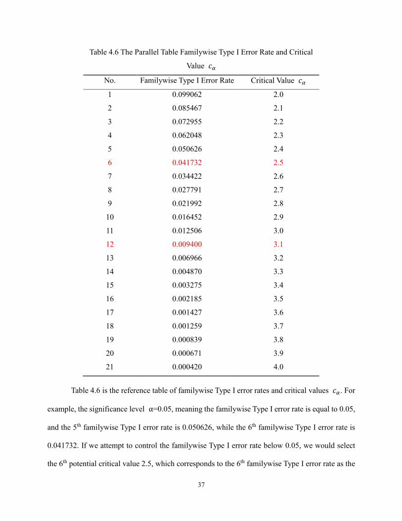
Table 4.6 The Parallel Table Familywise Type I Error Rate and Critical

Value 𝑐𝛼

No. Familywise Type I Error Rate Critical Value 𝑐𝛼

1 0.099062 2.0

2 0.085467 2.1

3 0.072955 2.2

4 0.062048 2.3

5 0.050626 2.4

6 0.041732 2.5

7 0.034422 2.6

8 0.027791 2.7

9 0.021992 2.8

10 0.016452 2.9

11 0.012506 3.0

12 0.009400 3.1

13 0.006966 3.2

14 0.004870 3.3

15 0.003275 3.4

16 0.002185 3.5

17 0.001427 3.6

18 0.001259 3.7

19 0.000839 3.8

20 0.000671 3.9

21 0.000420 4.0

Table 4.6 is the reference table of familywise Type I error rates and critical values 𝑐𝛼. For

example, the significance level α=0.05, meaning the familywise Type I error rate is equal to 0.05,

and the 5th familywise Type I error rate is 0.050626, while the 6th familywise Type I error rate is

0.041732. If we attempt to control the familywise Type I error rate below 0.05, we would select

the 6th potential critical value 2.5, which corresponds to the 6th familywise Type I error rate as the

38

critical value 𝑐𝛼. For α=0.01, the critical value should be 3.1 The selection procedure for other

significance level can reproduce the same process.

4.2.2 Application of Critical Value

After 30 repetitions, the average critical value 𝑐𝛼 for each moving sample size value

below the different significance level is listed as follows.

Table 4.7 The Average Critical Value 𝑐𝛼 at Different Significance Levels

Moving Sample Size 𝑐0.01 𝑐0.05 20 2.9 3.4

40 2.8 3.3

60 2.6 3.2

80 2.5 3.2

100 2.5 3.1

Figure 4.5 The Average Critical Value under Different Moving Sample Size

According to the Table 4.7 and the Figure 4.5, there are two main findings.

39

The first result to note is that the critical value 𝑐0.01is always greater than 𝑐0.05, which is

reasonable. The significance level α = 0.01 controls the familywise Type I error rate. Compared

with α = 0.05, the requirement for the probability of making the familywise Type I error is

enhanced, such that the detection procedure only could make the familywise Type I error at a lower

proportion. In another word, the detecting procedure might make fewer familywise Type I errors.

Therefore, the higher critical value 𝑐𝛼, that is the higher “threshold,” could reduce the sensitivity

of this program detection, make the detecting procedure being less sensitive, improve the accuracy

of identification, and make fewer mistakes when detecting compromised items.

The second result is that whatever the significance level might be, the critical value 𝑐𝛼

appears to be a minuscule decreasing trend along with the increase in the moving sample size, and

the relationship pattern between the critical value 𝑐𝛼 and the moving sample size is approximately

a flat line. This pattern illustrates that the value of moving sample size barely has any effect on the

critical value 𝑐𝛼 when the moving sample size is larger than 20.

These two values of the critical value (i.e., 𝑐0.01 and 𝑐0.05) would be directly applied to

the other two students’ latent trait conditions, the ability under linear growth and the ability with

periodical variation. For the other two scenarios, the results obtained here are used instead of

determining them again.

4.3 The Result and Analysis of Power Study

This section includes the results and a simple interpretation of the power study under three

different students’ latent trait scenarios.

40

4.3.1 The Regular Scenario

The average results of 30 replications under the θ ~ N (0,1) condition in this simulation

study are summarized as follows:

Table 4.8 The Average Results of 30 Replications Under the 𝜃~𝑁 (0,1) Condition

In Table 4.8, the “m” means moving sample size; “𝑐0.01” and “𝑐0.05” respectively stand for

the average critical value of detecting compromised items successfully at the significance level of

α = 0.01 and α = 0.05;“LAG_0.01”and“LAG_0.05” in the first line of Table 4.8 individually

signify the average lag between the change-point and the point of the detecting procedure which

recognizes the compromised items when the significance level is controlled at α = 0.01 and α =

0.05 by the program; “Power_0.01”and “Power_0.05” in the first line of Table 4.8 separately

indicate the average power of the detecting procedure used to identify the compromised items

perfectly when α = 0.01 and α = 0.05; and“NUMB”is marked for recording the number of

items monitored by the detecting procedure program.

There are two major parts in this simulation study. The first is determining the critical

value for the detecting procedure, and the second is investigating the power of this monitoring

program for different scenarios of students’ latent trait by imitating the compromised item. The

power study simulation begins after the general critical values had been defined, the moving

m 𝑐0.05 𝑐0.01 LAG_0.05 LAG_0.01 Power_0.05 Power_0.01 NUMB

20 2.9 3.4 120 203 1.000 0.950 396

40 2.8 3.3 85 105 1.000 1.000 396

60 2.6 3.2 70 79 1.000 1.000 396

80 2.5 3.2 57 68 1.000 1.000 396

100 2.5 3.1 44 52 1.000 1.000 396

41

sample size is pre-fixed, and the number of monitored items remains the same for different moving

sample size values.

For the 𝜃~𝑁(0,1) condition, the average number of monitored items was 396, that is,

there are 396 items which have been used more than 100 times (𝑛0 = 100). The item pool contains

only 400 items, nearly all of the items have been administrated 100 times, all of these items have

been monitored, and the usage rate of this item is favorable.

4.3.2 The Ability with Linear Growth Scenario

The average results for 30 replications under the ability with linear growth scenario in this

simulation study are summarized as follows:

Table 4.9 The Average Results of 30 Replications Under the Ability with Linear Growth

Scenario

m 𝑐0.05 𝑐0.01 LAG_0.05 LAG_0.01 Power_0.05 Power_0.0

1 NUMB

20 2.9 3.4 183 366 1.000 0.900 398

40 2.8 3.3 127 153 1.000 1.000 398

60 2.6 3.2 100 122 1.000 1.000 398

80 2.5 3.2 79 104 1.000 1.000 398

100 2.5 3.1 73 82 1.000 1.000 398

Table 4.9 shows that for the ability with linear growth scenario, the average number of

monitored items was 398. There are 398 items which have been used more than 100 times (𝑛0 =

100). Nearly all of the items have been monitored, and the usage rate of this item is satisfied.

4.3.3 The Ability with Periodical Variation Scenario

The average results of 30 replications under the ability with periodical variation scenario

in this simulation study are summarized below:

42

Table 4.10 The Average Results of 30 Replications Under the Ability with Periodical Variation

Scenario

m 𝑐0.05 𝑐0.01 LAG_0.05 LAG_0.01 Power_0.05 Power_0.0

1 NUMB

20 2.9 3.4 136 246 1.000 1.000 398

40 2.8 3.3 88 107 1.000 1.000 398

60 2.6 3.2 76 84 1.000 1.000 398

80 2.5 3.2 59 72 1.000 1.000 398

100 2.5 3.1 45 58 1.000 1.000 398

Table 4.10 shows that for the ability with periodical variation scenario, the average number

of monitored items was 398. 398 items have been used more than 100 times (𝑛0 = 100), and nearly

all of the items have been monitored, and the usage rate of this item is acceptable.

4.3.4 The Comparison

This simulation study seeks to test the robustness of this compromised item detection

procedure based on IRT under different students’ latent trait scenarios. In terms of robustness, two

indices are used to describe this character of the detecting process. The major index is the power

of the detecting procedure to identify the compromised items precisely. It can represent how

accurate the procedure might be. The assistant index is the lag, which is the distance between the

change-point and the point where the procedure flagged the compromised items. This could record

how long the procedure requires to recognize the compromised items. To put it differently, this

index can illustrate the efficiency of the procedure.

The summary table of all the scenarios appears below:

43

Table 4.11 The Summary Results of All the Simulation Scenarios

Index Scenario m=20 m=40 m=60 m=80 m=100

𝑐0.01 Same 3.4 3.3 3.2 3.2 3.1

𝑐0.05 Same 2.9 2.8 2.6 2.5 2.5

Power_0.01

Regular 0.950 1.000 1.000 1.000 1.000

Ability with linear growth 0.900 1.000 1.000 1.000 1.000

Ability with periodical variation 1.000 1.000 1.000 1.000 1.000

Power_0.05

Regular 1.000 1.000 1.000 1.000 1.000



LAG_0.01

Regular 203 105 79 68 52

Ability with linear growth 366 153 122 104 82

Ability with periodical variation 246 107 84 72 58

LAG_0.05

Regular 120 85 70 57 44



NUMB

Regular 396

Ability with linear growth 398

Ability with periodical variation 398

4.3.4.1 The Power Results

Table 4.12 The Summary Results for All the Simulation Scenarios


𝑐0.01 Same 3.4 3.3 3.2 3.2 3.1

𝑐0.05 Same 2.9 2.8 2.6 2.5 2.5

Power_0.01

Regular 0.950 1.000 1.000 1.000 1.000



Power_0.05

Regular 1.000 1.000 1.000 1.000 1.000



There are two significance levels in this simulation: α = 0.01 and α = 0.05. Meanwhile,

the program imitated three cases of students’ latent trait, and those separately are the 𝜃~𝑁(0,1)

condition, the ability with linear growth scenario, and the ability with periodical variation scenario.

Table 4.12 reflects that three critical results have been found. 1) Under both significance levels,

44

there is nearly no difference of power among the three different scenarios; 2) There is almost no

difference of the power between the two significance levels; 3) As the moving sample size

increases, the power for identifying the compromised items of the detection procedure would

remain 1. One possible reason for this phenomenon is that the leakage range r is 0.7, which is

means there are 70% potential test takers known the item in advance. Thus, there should be

sufficient deviation between the observed correct answers and the theoretical correct answers,

which makes the sequential procedure could identify the compromised items easily. In addition,

when m>30, the moving sample size is enough large and stable, so the result would be more

accurate and precise, and the power would be higher. In addition, for both two types of significance

levels, the power of detection procedure maintains a high quality (almost all of them are 1) all of

the time except when m=20. Therefore, this procedure maintains the detecting identification result

on a high level of accuracy, and is always robust.

To conduct a deep analysis of the difference regarding power with disparate experimental

settings, a paired-samples t test was computed.

• The t test for the difference in power involved two different significance levels

Table 4.13 The Paired-Samples t Test Result for Power of Regular and Linear Growth (R to L)

α Mean Sd. Std Error

Mean.

95% Confidence

Interval t df Sig.

(2-tailed) Lower Upper

0.01 0.0100 0.02236 0.0100 -0.0178 0.0378 1.000 4 0.374

Table 4.13 generalized the t test results for the power for regular and ability with linear

growth scenarios, and there is no distinct difference between these two scenarios when α = 0.01

(Sig.=0.374). For α = 0.05, there is no difference of power between these two scenarios in terms

of all the powers are 1. Hence, the ability with linear growth scenario could not affect the

performance of the critical value settled down in the 𝜃~𝑁(0,1) condition.

45

Table 4.14 The Paired-Samples t Test Result for Power of Regular and Periodical Variations (R

to P)


Mean.

95% Confidence

Interval t df Sig.


0.01 -0.0100 0.02236 0.0100 -0.0378 0.0178 1.000 4 0.374

The t test results of the power for regular and ability with periodical variation scenarios are

summed up in Table 4.14. There is no significantly difference between these two scenario

experimental settings when α = 0.01 (Sig.=0.374). There is still no difference of power for α =

0.05. Therefore, the critical value fixed in the 𝜃~𝑁(0,1) condition still could work well when

the scenario is under the ability with periodical variation scenario.

In conclusion, both of the scenarios (the ability with linear growth scenario, and the ability

with periodical variation scenario) will not introduce an influence on the performance of the critical

value which had been determined under the 𝜃~𝑁(0,1) condition.

• The t test for the difference of power among three scenarios

Table 4.15 The Paired-Samples t Test of Power Result for Significance Levels (0.01 to 0.05)

Scenario Mean Sd. Std Error

Mean.

95% Confidence

Interval t df

Sig.

(2-

tailed) Lower Upper

Regular. 0.0100 0.02236 0.0100 -0.0178 0.0378 1.000 4 0.374

Increase. 0.0200 0.04472 0.0200 -0.0355 0.0755 1.000 4 0.374

Table 4.15 lists the results of the t test for power between two significance level under two

scenario settings (the power is always 1 under the periodical variation scenario). There is no

difference between these two significant levels. Actually, the power of correct detection at α =

0.05 should larger than it at α = 0.01, because the power should be larger when α value is

46

bigger. However, it might because the leakage range is 0.7, and it could not appear the difference

at this level.

If the sequential detection procedure flagged a simulated compromised item as a

compromised item before the change-point (that is a familywise Type I error), and this item is

exactly the mimicked compromised item, it would not be a compromised item anymore, because

we could not know whether an item would be or not to be a compromised item in advance.

4.3.4.2 The Results and Analysis of Lag

Table 4.16 The Summary Results of All the Simulation Scenarios


𝑐0.01 Same 3.4 3.3 3.2 3.2 3.1

𝑐0.05 Same 2.9 2.8 2.6 2.5 2.5

LAG_0.01

Regular 203 105 79 68 52



LAG_0.05

Regular 120 85 70 57 44



47

Figure 4.6 The Change Pattern of Lag under Three Scenarios

In addition, there are two significance levels, α = 0.01 and 0.05, and three true ability

conditions. Synthesizing the results reported in Table 4.16 and Figure 4.6, there are also three

important findings. (1) For each significance level, there might be difference of lag among three

different scenarios; (2) There might not be difference of the lag between the two significance levels

under each latent trait scenario; (3) Along with the increase in moving sample size, the lag exhibits

a curve decreasing trend, and the curve sharply goes down between m = 20 and m = 40, and the

decreasing trend of those curves become slow along with the moving sample size increasing from

40.

In presenting the decreasing pattern, the accuracy of the detecting procedure may be the

cause. As mentioned in the power results part before, larger moving sample size means the more

representative the sample, which means the detection procedure could be more sensitive for larger

moving sample size.

0

50

100

150

200

250

300

350

400

20 40 60 80 100

Regular_0.05 Linear Growth_0.05 Periodical Variation_0.05

Regular_0.01 Linear Growth_0.01 Periodical Variation_0.01

48

Therefore, the procedure requires taking fewer time to run fewer tests to identify the

compromised items. There are two groups of students in a moving sample regularly; one is the

“honest” student group, and the other one is the “dishonest” student group. The probability of the

“dishonest” students answering the compromised items correctly is greater than for the “honest”

students. As regards the “dishonest” students in a moving sample, the statistic �̂�𝑛𝑚 would be

larger, and the procedure would catch them more readily. If all of the “dishonest” students are in a

moving sample, the �̂�𝑛𝑚 could get to the peak. For a larger moving sample size, the sequential

detection procedure could cost fewer test takers to flag a compromised item, even not to get to the

peak of �̂�𝑛𝑚.

Furthermore, the fluctuating range of lag among the three scenario settings for α = 0.01

is (50, 360), and for α = 0.05 is (40, 180). The space between the lower bound and the upper

bound is, respectively, around 310 and 140. There are 5,000 simulated test takers in this simulation,

so the floating on this level is acceptable. It could show that this detection procedure is efficient,

and it could distinguish a compromised item from others in a relatively short time.

As regards further verification of these findings concerning the difference of lag under

different simulation conditions, several paired-samples t tests have been run.

• The t test for the difference of lag above two significance levels

Table 4.17 The Paired-Samples t Test Result for Lag of Regular and Ability with Linear

Growth (L to R)


Mean.

95% Confidence

Interval t df Sig.


0.01 64.00 55.7629 24.9379 -5.2388 133.2388 2.566 4 0.062

0.05 37.20 16.1152 7.2069 17.1903 57.2097 5.162 4 0.007

49

Table 4.17 shows t test results of the lag for the 𝜃~𝑁(0,1) condition and the ability with

linear growth scenario, and there is statistical evidence show that there is difference between these

two scenarios for two significant levels (α = 0.01: Sig.=0.062; α = 0.05: Sig.=0.007). Thus, the

sequential detection procedure would take more time to identify a compromised item under the

ability with linear growth scenario.

Table 4.18 The Paired-Samples t Test Result for Lag of Regular and Periodical Variation (P to

R)


Mean.

95% Confidence

Interval t df Sig.


0.01 12.00 17.3925 7.7782 -9.5957 33.5957 1.543 4 0.198

0.05 5.600 6.1073 2.7313 -1.9833 13.1833 2.050 4 0.110

Table 4.18 summarized the t test results of the lag for Regular and the ability with

periodical variation scenario. There is no difference of lag between the two scenario settings. That

means that the general critical values can work as well as it works under the 𝜃~𝑁(0,1) condition.

In a word, the general critical values have the same performance with the 𝜃~𝑁(0,1)

condition when the students’ latent trait in obeying the settings of the ability with periodical

variation scenario, while it need more time to work in the same effect following the ability with

linear growth scenario.

• The t test for the difference of lag among the three scenarios

Table 4.19 The Paired-Samples t Test of Lag Result for Significance Level (0.01 to 0.05)

Scenario. Mean Sd. Std Error

Mean.

95% Confidence

Interval t df

Sig.

(2-

tailed) Lower Upper

Regular. 26.20 32.1045 14.3576 -13.6630 66.0630 1.825 4 0.142

Linear. 53.00 72.9897 32.6420 -37.6287 143.6287 1.624 4 0.180

Periodical. 32.60 43.4431 19.4283 -21.3417 86.5417 1.678 4 0.169

50

According to Table 4.19, the lag of α = 0.01 is not significantly larger than α = 0.05,

and all of the t test results are not significant (Sig.>0.1). Therefore, the significance level would

not impact the performance of lag under each latent trait scenario.

51

CHAPTER 5: SUMMARY AND DIRECTIONS FOR FUTURE RESEARCH

5.1 Conclusion

Based on analysis in the last chapter, below are the major conclusions found from the

simulation study.

5.1.1 For the Scenario Imitation

(1) In comparing the 𝜃~𝑁(0,1) condition and the ability with periodical variation

scenarios, the normal distribution curve of the ability with linear growth scenario is to the right,

and its mean and median are larger than the 𝜃~𝑁(0,1) and periodical variation condition.

(2) The dispersion level of the ability with periodical variation scenario is greater than the

others, the peak of the normal distribution curve of latent trait under the ability with periodical

variation condition is lower than the other two, the shape is flatter, and the standard deviation is

larger.

(3) The estimated ability is highly correlated to the true ability, and the precision of latent

trait evaluation is not damaged too much by the imitated compromised items under the progressive

item selection method.

5.1.2 For the Critical Value 𝒄𝜶

(1) The varying range of the potential critical value 𝑐𝛼 is (2, 4) by step at 0.1, and there

are 21 possible critical value 𝑐𝛼 s among this range. These 21 values could cover the regular

significance level, which are α=0.01, 0.05.

(2) The critical value 𝑐0.01 is always higher than 𝑐0.05.

52

(3) Whatever the significance level is, the critical value 𝑐𝛼 shows a minuscule deceasing

trend along with an increase of the moving sample size. The value of the moving sample size has

little effect on the critical value 𝑐𝛼 when the moving sample size is greater than 20.

5.1.3 The Number of Monitored Items

For all three scenarios, nearly all the items were monitored, and the usage rate of this item

pool is satisfied.

5.1.4 Power

(1) Under both significance levels, there is nearly no difference of power among these three

different scenarios. The ability with linear growth scenario and the ability with periodical variation

scenario will not affect the performance of the general critical value which was determined under

the 𝜃~𝑁(0,1) condition. The detection procedure is robust under the power index accessing, and

it would not be affected by the different scenarios in terms of power.

(2) There is no obvious difference in the power between the two significance levels, that is

α = 0.01 and α = 0.05.

(3) Along with the increase in the moving sample size, the power for verdict of the detection

procedure would almost stay at 1, and the detection procedure could keep such high quality of

power all of the time. Therefore, this procedure maintains the detecting identification result at a

high accuracy level, and is always robust when the moving sample size is sufficiently large.

5.1.5 The Lag

(1) For the two significance levels, there were statistically differences for lags among the

53

three different scenarios. If the critical value has the same performance with the 𝜃~𝑁(0,1)

condition, it would take on a little bit longer lag when the students’ latent trait obeys the settings

of the ability with linear growth scenario, while it could work the same effect following both

regular and the ability with periodical variation scenarios. The detection procedure is relatively

robust under the lag index evaluating, and it would be affected slightly when the latent trait under

the ability with linear growth scenario.

(2) There is no obvious difference of the lag between the two significance levels, and the

lag of α = 0.01 is not significantly larger than α = 0.05.

(3) When the moving sample size increases, the lag exhibits a curved decreasing trend, and

the pattern is going down extremely first and then becoming slowly. Moreover, the detection

procedure is efficient, and it could distinguish a compromised item from other items in a relatively

short lag (for α = 0.01, linger in (50, 360); for α = 0.05, linger in (40, 180)).

5.2 Discussion

5.2.1 For the Scenario Imitation

The distribution of students’ latent trait would not affect estimates of their true abilities

using Item Response Theory. This sequential detecting procedure is also based on the IRT, as a

new method of detecting the compromised items. There were not many articles emphasized on the

influence of students’ latent trait distribution. Through this simulation study, it moves a single step

forward to the true ability distribution influence in the experimental angle.

54

5.2.2 The Critical Value 𝒄𝜶

This simulation study has two major parts. The first part of the program imitates a whole

process of computerized adaptive testing by simulating the true ability of students. After generating

the responses of students, the program calculates the hypothesis test statistic �̂�𝑛𝑚，and compares

it with a serial potential critical value 𝑐𝛼s one by one, then gets the reference table between the

familywise Type I error rate and the critical value 𝑐𝛼. Depending on the research needs, a suitable

critical value 𝑐𝛼 will be selected. After that, the first part of the simulation is finished. After the

first part, the program will modify the probability of the students answering the compromised

items correctly to mimic the compromised items, and then re-run the detecting procedure again

under each student’s latent trait scenarios. Finally, the detecting procedure would be accessed by

the evaluation index of power and lag.

By returning back to the essence of the R-coding, each student’s latent trait value would

be homogeneous with one set of critical values (and for two significance levels) which are fitted

for current simulation settings. When α = 0.05, there is a critical value 𝑐0.05, and there is also a

critical value 𝑐0.01 for α = 0.01. These two critical values refer to a set of critical values. That is,

there are two values in one set of critical values corresponding to two individual significance levels.

As regards the 𝜃~𝑁(0,1) condition, the program would apply to every set of critical values to

proceed through the hypothesis test under each moving sample size level. All of the above is a

one-time simulation process, and it will be repeated 30 times for the 𝜃~𝑁(0,1) condition to

determine a set of general critical values. After the set of general critical values (the average of

critical values for the 30 replications) is fixed, this set of critical values would be directly

introduced into the other scenarios: these are the ability with linear growth scenario and the ability

with periodical variation scenario. The simulation requires 30 replications for each scenario.

55

The process illustrated above allow us to learn that a set of critical values would be

generated from the program after a one-time test in each time simulation, and this is according to

the actual scenarios. For real computerized adaptive testing, this procedure should be conducted

once during a fixed period which is shorter than the period the item pool would be employed. For

example, after one day or two days of testing, or a fixed number of test takers, the detecting

procedure could be applied at that point. At that moment, there is a considerable number of

responses of the students in the computerized adaptive testing system, and estimates of their latent

trait. Based on the existing data information, the program could define a set of general critical

values which could be used in tests in the future.

This study focused on the situation that items were compromised because the students

shared items after an item pool had been used, but does not consider the other conditions, such as

whether the items were stolen before the test administration. In the simulation context, the

procedure needs a pre-test or a first test to specify the set of general critical values. For example,

the GRE and the TPEFL IBT are computer-based tests, and the number of seat for every time test

is fixed. Given that a new item pool begins to be used, the first test would contain 1000 test takers,

and the items’ information could not be compromised during the test. Therefore, this test could be

regarded as a test which does not involve the compromised items. The detection procedure could

define the set of general critical values according to the data derived from this test. The detection

procedure could bring that set of general critical values into later tests.

The circumstance above show that the detection procedure used in this simulation could

monitor the computerized adaptive testing program after the computerized adaptive testing has

been in operation for a short time period which is smaller than the usage period of the item pool.

It could not follow up every test taker and the item during the time that testing has been going on.

56

5.2.3 The Power Study

The power is equal to one minus the Type Ⅱ error rate. It is necessary to probe other factors

which could affect the power of this procedure, which could push the improvement of this

sequential detection procedure. A possible direction might be investigating the relationship

between the moving sample size and the power.

5.2.4 The Lag

The nonexistent lags (lag=NA) were excluded when calculating the final lag.

In the pre-simulation experiment, it is not difficult to determine that the value of lag could

be zero, positive, and nonexistent. If the detection procedure has identified the compromised items

before the change-point, which means that the items have not been compromised. The items have

not been compromised, and the detecting procedure reports them wrongly, which makes it a

familywise Type I error. It is a false “correct judgement,” or it could be called as a false “positive

decision.” For that situation, the mimicked compromised item should not be the compromised item

anymore, because we could not know a compromised item before it leaked. Therefore, it will be

removed from the imitated compromised item group. When the lag is zero, it means that the

detecting procedure recognizes the compromised items at the change-point, and it is a correct

identification. When the lag is positive, it means that the detecting procedure finds those

compromised items after the change-point, and it is the correct decision. When the lag is

nonexistence, it means that the detection procedure does not find the compromised items after the

change-point. The compromised items have not been detected, which is a Type II error, and a false

“negative decision.”

57

Given the above statement, it is clear that the detection procedure makes a Type II error

when the lag is nonexistent. The program records only the zero and positive lag situations, which

is the detection procedure flags the compromised items correctly, and makes the right “positive

judgement” decision.

5.3 Future Directions for Research

Several research directions would deserve the further attention.

5.3.1 Scenario Imitation

In this simulation, there are three mimicked scenarios of the students’ true ability

distribution. Based on the literature review, there are few studies of this field. In the future, the

researchers could review or constitute more studies to figure out the changing mechanism of

scenario for students’ latent trait in different large-scale tests, and it might bring to light more

esoteric research questions and directions.

Moreover, Chang and Ying (1996) expressed the KL information function, and proposed

a global information approach which is improving the bias and mean squared error. The posterior

Kullback-Leibler method (KLP) could balance the larger KL values at extreme θ level by

imposing the posterior density distribution (Chen, Ankenmann, & Chang, 2000). This method

could reduce the RMSE, so the accuracy of it is better than other item selection strategy (J. R.

Barrada et al., 2010; J. R. n. Barrada, Olea, Ponsoda, & Abad, 2009). In terms of mimicking the

compromised items, the program of this simulation needs an item selection strategy with an

outstanding performance on estimation accuracy and test security. For the future research, it is

58

valuable to try a better item selection function, such as KLP, to improve the performance of this

sequential procedure for detecting the compromised items in computerized adaptive testing.

5.3.2 Critical Value 𝒄𝜶

(1) Develop this procedure into a real-time higher-order version. Let the detection

procedure follow up every test taker and items during the time when the testing has been going on.

The higher-order version detection procedure could define in real-time the critical values according

to the current responses of test takers and monitor items usage status. The identification of general

critical values be a dynamic process. The application of the detection procedure could simplify the

pre-test process of determining the critical values.

At the same time, an ancillary item pool could be built, which includes mothballed items

that possess the same item character parameters as the original item pool. Once the real-time

higher-order version procedure flagged a compromised item, the computerized adaptive testing

system would immediately select the item which possesses the exact same item character

parameters as does the compromised item, and replace the compromised item during the test

program operations.

(2) Explore the factors which influence the critical values, and their incidences. It could

help define a set of critical values which could be employed for a long time in real circumstances.

That will help this procedure be applied to real situations.

5.3.3 Further Power Study

(1) Future research could inspect the influence factors for power in a multi-dimensional

manner, such as the moving the sample size, the occasions when items have been compromised,

59

and how deeply the items have been compromised.

(2) In this simulation study, the only situation considered is that the compromised items

would provide benefits for the students, which means the computerized adaptive testing system

would overestimate the ability of students who benefit from the compromised items. However, in

real situations, the compromised items might introduce some negative affection for student’s due

to the memory effect, the time lapsing, or other possible factors. It could decrease the probability

of the students answering the compromised items correctly, and compel the computerized adaptive

testing to underestimate the true ability of students. Hence, in future studies, the underestimated

situation could be considered for testing the robustness of this detection procedure.

(3) This simulation study only tests the situation where the compromise of the simulated

compromised items occurs after the detection procedure has begun, and it could be a reasonable

direction for the compromise to occur before the detecting procedure has been started, or exactly

at the point when the procedure begins.

5.3.4 About Lag

In this simulation, the characteristic of the lag could be an index for whether or not the

detecting procedure could identify the compromised items. As regards future research, this type of

“pure” lag, where only the zero and positive lags are recorded, could be adopted continuously to

maintain the efficiency of the detecting procedure.

5.3.5 About Program Code

As regards this simulation study, the program is developed based on R language, but it is

too slow to finish the simulation. For future simulations, the speed of simulation and analysis could

60

be improved using other computer languages, such as C++, or Fortran, which are more efficient

and faster and could enhance the efficiency of analogous simulation research.

61

REFERENCES

Allen, M. J., & Yen, W. M. (2001). Introduction to measurement theory: Waveland Press.

Anscombe, F., Godwin, H., & Plackett, R. (1947). Methods of deferred sentencing in testing the

fraction defective of a continuous output. Supplement to the Journal of the Royal Statistical

Society, 198-217.

Barrada, J. R., Olea, J., Ponsoda, V., & Abad, F. J. (2008). Incorporating randomness in the Fisher

information for improving item ‐ exposure control in CATs. British Journal of

Mathematical and Statistical Psychology, 61(2), 493-513.

Barrada, J. R., Olea, J., Ponsoda, V., & Abad, F. J. (2010). A method for the comparison of item

selection rules in computerized adaptive testing. Applied Psychological Measurement,

34(6), 438-452.

Barrada, J. R. n., Olea, J., Ponsoda, V., & Abad, F. J. (2009). Item selection rules in Computerized

Adaptive Testing: Accuracy and security. Methodology, 5(1), 7-17.

Birnbaum, A. (1968). Some latent trait models and their use in inferring an examinee's ability. In

F. M. Lord & M. R. Novick (Eds.), Statistical theories of mental test scores. Reading, MA:

Adison-Wesley.

Bock, R. D., & Mislevy, R. J. (1982). Adaptive EAP estimation of ability in a microcomputer

environment. Applied Psychological Measurement, 6(4), 431-444.

doi:10.1177/014662168200600405

Carlstein, E. (1988). Nonparametric change-point estimation. The Annals of Statistics, 188-197.

Chang, H.-H., & Ying, Z. (1996). A global information approach to computerized adaptive testing.

Applied Psychological Measurement, 20(3), 213-229.

62

Chang, H.-H., & Zhang, J. (2002). Hypergeometric family and item overlap rates in computerized

adaptive testing. Psychometrika, 67(3), 387-398.

Chang, H.-H., & Zhang, J. (2003, April). Assessing CAT security breaches by the item pooling

index. Paper presented at the annual meeting of National Council on Measurement in

Education, Chicago, IL.

Chen, S.-Y., Ankenmann, R. D., & Chang, H.-H. (2000). A comparison of item selection rules at

the early stages of computerized adaptive testing. Applied Psychological Measurement,

24(3), 241-255.

Cheng, L. (2016). The application of rasch model in the college entrance examination - for example,

the change of the physical ability level of candidates in different years. Theory and Practice

of Education, 36(5), 13-15.

Downing, S. M., & Haladyna, T. M. (2006). Handbook of test development: Lawrence Erlbaum

Associates Publishers.

Georgiadou, E. G., Triantafillou, E., & Economides, A. A. (2007). A review of item exposure

control strategies for computerized adaptive testing developed from 1983 to 2005. The

Journal of Technology, Learning and Assessment, 5(8).

Hu, Z. (2010). Psychological statistics: Higher Education Press.

Keppel, G., & Wickens, T. (2004). Design and analysis: A researcher’s handbook. 4th ed. : Upper

Saddle River (NJ): Pearson Prentice Hall. .

Lord, F. M. (1971a). Robbins-Monro procedures for tailored testing. Educational and

Psychological Measurement, 31(1), 3-31.

Lord, F. M. (1971b). Tailored testing, an application of stochastic approximation. Journal of the

American Statistical Association, 66(336), 707-711.

63

Lord, F. M. (1971c). A theoretical study of the measurement effectiveness of flexilevel tests.

Educational and Psychological Measurement, 31(4), 805-813.

Lord, F. M. (1980). Applications of item response theory to practical testing problems: Routledge.

Lorden, G. (1971). Procedures for reacting to a change in distribution. The Annals of Mathematical

Statistics, 1897-1908.

Luo, Z. (2012). Item response theory: Beijing Normal University Publishing House.

Mao, X., & Xin, T. (2011). Item selection method in computerized adaptive testing. Advances in

Psychological Science, 19(10), 1552-1562.

Medina, N., & Neill, D. M. (1988). Fallout from the testing explosion: How 100 million

standardized exams undermine equity and excellence in America's public schools.

Page, E. S. (1954). Continuous inspection schemes. Biometrika, 41(1/2), 100-115.

Parshall, C. G., Spray, J. A., Kalohn, J. C., & Davey, T. (2002). Issues in innovative item types

Practical Considerations in Computer-Based Testing (pp. 70-91): Springer.

Pollak, M. (1985). Optimal detection of a change in distribution. The Annals of Statistics, 206-227.

Revuelta, J., & Ponsoda, V. (1998). A comparison of item exposure control methods in

computerized adaptive testing. Journal of Educational Measurement, 35(4), 311-327.

Siegmund, D. (1986). Boundary crossing probabilities and statistical applications. The Annals of

Statistics, 361-404.

Wainer, H. (2000). Computerized adaptive testing: Wiley Online Library.

Yi, Q., Zhang, J., & Chang, H.-H. (2006). Severity of organized item theft in computerized

adaptive testing: an empirical study. ETS Research Report Series, 2006(2).

Yi, Q., Zhang, J., & Chang, H.-H. (2008). Severity of organized item theft in computerized

adaptive testing: A simulation study. Applied Psychological Measurement, 32(7), 543-558.

64

Zhang, J. (2014). A sequential procedure for detecting compromised items in the item pool of a

CAT system. Applied Psychological Measurement, 38(2), 87-104.

doi:10.1177/0146621613510062

Zhang, J., Cao, C., & Jie, Y. (2017). Robustness of CTT- and IRT-based sequential procedures for

detecting compromised items in CAT. China Examinations, 2, 20-32.

Zhang, J., Chang, H.-H., & Yi, Q. (2012). Comparing single-pool and multiple-pool designs

regarding test security in computerized testing. Behavior research methods, 44(3), 742-752.

Zhang, J., & Li, J. (2016). Monitoring items in real time to enhance CAT security. Journal of

Educational Measurement, 53(2), 131-151. doi:10.1111/jedm.12104

Documents

© 2017 CANXI CAO