Embed Size (px)
Citation preview

ii
iii
WorldwideIntegralCalculuswith infinite series
David B. Massey
with select exercises and answers by Gabriel Merton and Ryan Malloy,
select illustrations by Eugene Saletan,
and select video solutions by Michael Garcia and Ryan Malloy

iv
c©2009, Worldwide Center of Mathematics, LLC
Contents
0.1 Preface . . . . . . . . . . . . . . . . . . . . . . . . . . . . . . . . . . . . . . . . . ix
1 Anti-differentiation: the Indefinite Integral 1
1.1 Basic Anti-Differentiation . . . . . . . . . . . . . . . . . . . . . . . . . . . . . . . 2
1.1.1 Exercises . . . . . . . . . . . . . . . . . . . . . . . . . . . . . . . . . . . . 21
1.2 Special Trig. Integrals and Trig. Substitutions . . . . . . . . . . . . . . . . . . . 29
1.2.1 Exercises . . . . . . . . . . . . . . . . . . . . . . . . . . . . . . . . . . . . 35
1.3 Integration by Partial Fractions . . . . . . . . . . . . . . . . . . . . . . . . . . . . 39
1.3.1 Exercises . . . . . . . . . . . . . . . . . . . . . . . . . . . . . . . . . . . . 51
1.4 Integration using Hyperbolic Sine and Cosine . . . . . . . . . . . . . . . . . . . . 57
1.4.1 Exercises . . . . . . . . . . . . . . . . . . . . . . . . . . . . . . . . . . . . 62
2 Continuous sums: the Definite Integral 67
2.1 Sums and Differences . . . . . . . . . . . . . . . . . . . . . . . . . . . . . . . . . . 68
2.1.1 Exercises . . . . . . . . . . . . . . . . . . . . . . . . . . . . . . . . . . . . 76
2.2 Prelude to the Definite Integral . . . . . . . . . . . . . . . . . . . . . . . . . . . . 83
2.2.1 Exercises . . . . . . . . . . . . . . . . . . . . . . . . . . . . . . . . . . . . 100
2.3 The Definite Integral . . . . . . . . . . . . . . . . . . . . . . . . . . . . . . . . . . 107
2.3.1 Exercises . . . . . . . . . . . . . . . . . . . . . . . . . . . . . . . . . . . . 134
2.4 The Fundamental Theorem of Calculus . . . . . . . . . . . . . . . . . . . . . . . . 139
2.4.1 Exercises . . . . . . . . . . . . . . . . . . . . . . . . . . . . . . . . . . . . 153
2.5 Improper Integrals . . . . . . . . . . . . . . . . . . . . . . . . . . . . . . . . . . . 159
2.5.1 Exercises . . . . . . . . . . . . . . . . . . . . . . . . . . . . . . . . . . . . 173
v
vi CONTENTS
2.6 Numerical Techniques . . . . . . . . . . . . . . . . . . . . . . . . . . . . . . . . . 180
2.6.1 Exercises . . . . . . . . . . . . . . . . . . . . . . . . . . . . . . . . . . . . 194
Appendix 2.A Technical Matters . . . . . . . . . . . . . . . . . . . . . . . . . . . . . . 201
3 Applications of Integration 215
3.1 Displacement and Distance Traveled . . . . . . . . . . . . . . . . . . . . . . . . . 216
3.1.1 Exercises . . . . . . . . . . . . . . . . . . . . . . . . . . . . . . . . . . . . 223
3.2 Area in the Plane . . . . . . . . . . . . . . . . . . . . . . . . . . . . . . . . . . . . 228
3.2.1 Exercises . . . . . . . . . . . . . . . . . . . . . . . . . . . . . . . . . . . . 242
3.3 Distance Traveled in Space and Arc Length . . . . . . . . . . . . . . . . . . . . . 249
3.3.1 Exercises . . . . . . . . . . . . . . . . . . . . . . . . . . . . . . . . . . . . 269
3.4 Area Swept Out and Polar Coordinates . . . . . . . . . . . . . . . . . . . . . . . 276
3.4.1 Exercises . . . . . . . . . . . . . . . . . . . . . . . . . . . . . . . . . . . . 289
3.5 Volume . . . . . . . . . . . . . . . . . . . . . . . . . . . . . . . . . . . . . . . . . 294
3.5.1 Exercises . . . . . . . . . . . . . . . . . . . . . . . . . . . . . . . . . . . . 314
3.6 Surface Area . . . . . . . . . . . . . . . . . . . . . . . . . . . . . . . . . . . . . . 321
3.6.1 Exercises . . . . . . . . . . . . . . . . . . . . . . . . . . . . . . . . . . . . 329
3.7 Mass and Density . . . . . . . . . . . . . . . . . . . . . . . . . . . . . . . . . . . . 334
3.7.1 Exercises . . . . . . . . . . . . . . . . . . . . . . . . . . . . . . . . . . . . 343
3.8 Centers of Mass and Moments . . . . . . . . . . . . . . . . . . . . . . . . . . . . . 348
3.8.1 Exercises . . . . . . . . . . . . . . . . . . . . . . . . . . . . . . . . . . . . 361
3.9 Work and Energy . . . . . . . . . . . . . . . . . . . . . . . . . . . . . . . . . . . . 366
3.9.1 Exercises . . . . . . . . . . . . . . . . . . . . . . . . . . . . . . . . . . . . 380
3.10 Hydrostatic Pressure . . . . . . . . . . . . . . . . . . . . . . . . . . . . . . . . . . 385
3.10.1 Exercises . . . . . . . . . . . . . . . . . . . . . . . . . . . . . . . . . . . . 389
4 Polynomials and Power Series 393
4.1 Approximating Polynomials . . . . . . . . . . . . . . . . . . . . . . . . . . . . . . 395
4.1.1 Exercises . . . . . . . . . . . . . . . . . . . . . . . . . . . . . . . . . . . . 405
4.2 Approximation of Functions . . . . . . . . . . . . . . . . . . . . . . . . . . . . . . 408
CONTENTS vii
4.2.1 Exercises . . . . . . . . . . . . . . . . . . . . . . . . . . . . . . . . . . . . 422
4.3 Error in Approximation . . . . . . . . . . . . . . . . . . . . . . . . . . . . . . . . 426
4.3.1 Exercises . . . . . . . . . . . . . . . . . . . . . . . . . . . . . . . . . . . . 438
4.4 Functions as Power Series . . . . . . . . . . . . . . . . . . . . . . . . . . . . . . . 444
4.4.1 Exercises . . . . . . . . . . . . . . . . . . . . . . . . . . . . . . . . . . . . 458
4.5 Power Series as Functions I . . . . . . . . . . . . . . . . . . . . . . . . . . . . . . 462
4.5.1 Exercises . . . . . . . . . . . . . . . . . . . . . . . . . . . . . . . . . . . . 482
4.6 Power Series as Functions II . . . . . . . . . . . . . . . . . . . . . . . . . . . . . . 487
4.6.1 Exercises . . . . . . . . . . . . . . . . . . . . . . . . . . . . . . . . . . . . 510
4.7 Power Series Solutions . . . . . . . . . . . . . . . . . . . . . . . . . . . . . . . . . 515
4.7.1 Exercises . . . . . . . . . . . . . . . . . . . . . . . . . . . . . . . . . . . . 526
Appendix 4.A Technical Matters . . . . . . . . . . . . . . . . . . . . . . . . . . . . . . 528
5 Theorems on Sequences and Series 529
5.1 Theorems on Sequences . . . . . . . . . . . . . . . . . . . . . . . . . . . . . . . . 530
5.1.1 Exercises . . . . . . . . . . . . . . . . . . . . . . . . . . . . . . . . . . . . 544
5.2 Basic Theorems on Series . . . . . . . . . . . . . . . . . . . . . . . . . . . . . . . 548
5.2.1 Exercises . . . . . . . . . . . . . . . . . . . . . . . . . . . . . . . . . . . . 566
5.3 Non-negative Series . . . . . . . . . . . . . . . . . . . . . . . . . . . . . . . . . . . 572
5.3.1 Exercises . . . . . . . . . . . . . . . . . . . . . . . . . . . . . . . . . . . . 592
5.4 Series with Positive and Negative Terms . . . . . . . . . . . . . . . . . . . . . . . 596
5.4.1 Exercises . . . . . . . . . . . . . . . . . . . . . . . . . . . . . . . . . . . . 611
Appendix A An Introduction to Vectors and Motion 615
Appendix B Tables of Integration Formulas 623
Appendix C Answers to Odd-Numbered Exercises 627
Bibliography 649
Index 651

viii CONTENTS
About the Author 657
0.1. PREFACE ix
0.1 Preface
Welcome to the Worldwide Integral Calculus textbook; the second textbook from the WorldwideCenter of Mathematics.
Our goal with this textbook is, of course, to help you learn Integral Calculus (and powerseries methods) – the Calculus of integration. But why publish a new textbook for this purposewhen so many already exist? There are several reasons why we believe that our textbook is avast improvement over those already in existence.
• Even if this textbook is used as a classic printed text, we believe that the exposition, expla-nations, examples, and layout are superior to every other Calculus textbook. We have tried towrite the text as we would speak the material in class; though, of course, the book contains farmore details than we would normally present in class. In the book, we emphasize intuitive ideasin conjunction with rigorous statements of theorems, and provide a large number of illustrativeexamples. Where we think it will be helpful to you, we include proofs, or sketches of proofs,in the midst of the sections, but the extremely technical proofs are contained in the TechnicalMatters appendices to chapters, or are contained in referenced external sources. This greatlyimproves the overall readability of our textbook, while still allowing us to give mathematicallyprecise definitions and statements of theorems.
• Our textbook is an Adobe pdf file, with linked/embedded/accompanying video content, an-notations, and hyperlinks. With the videos contained in the supplementary files, you effectivelypossess not only a textbook, but also an online/electronic version of a course in Integral Cal-culus. Depending on the version of the files that you are using, clicking on the video frame tothe right of each section title will either open an online, or an embedded, or a locally installedvideo lecture on that section. The annotations replace classic footnotes, without affecting thereadability or formatting of the other text. The hyperlinks enable you to quickly jump to areference elsewhere in the text, and then jump back to where you were.
• The pdf format of our textbook makes it incredibly portable. You can carry it on a laptopcomputer, on many handheld devices, e.g., an iPad, or can print any desired pages.
• Rather than force you to buy new editions of textbooks to obtain corrections and minorrevisions, updates of this textbook are distributed free of cost.
• Because we have no print or dvd costs for the electronic version of this book and/or videos,we can make them available for download at an extremely low price. In addition, the printed,bound copies of this text and/or disks with the electronic files are priced as low as possible, tohelp reduce the burden of excessive textbook prices.
x PREFACE
In this book, we assume you are already familiar with Differential Calculus. Specifically,we assume that you know the definition of the derivative of a function, that it represents theinstantaneous rate of change, and that you know the “rules” for calculating derivatives. We willalso need l’Hopital’s Rule and parameterized curves. Referring to the Worldwide DifferentialCalculus textbook [2], this means that you should know the contents of Chapters 1 and 2, Section3.5, and Appendix A.
Our discussion of definite integrals, and their applications, is fairly traditional. However, ourapproach to infinite series is somewhat unusual. Our approach is motivated by two factors. First,we believe that the primary use that students will have for infinite series, outside of a Calculusclass, is that many important functions have convergent power series representations, and thesepower series representations allow the student to mathematically manipulate and estimate thefunctions involved, in ways that would be difficult/impossible without power series. Second,statistical data that we collected over several years has made it clear that, in general, studentsdo not grasp the basic idea that, when x is close to zero, smaller powers of x are more significantthan larger powers of x in a power series or, even, in a polynomial function.
Consequently, we place emphasis on polynomial approximations and power series represen-tations for functions, and, in a sense, view the classic convergence tests for sequences and seriesof constants as the “technical details” required to understand power series. We still include achapter, Chapter 5, on sequences and series of constants, but that chapter comes after Chap-ter 4, which is on power series and approximating functions with polynomials. We firmly believethat this ordering of topics is better for the student and for applications, even though it mayseem a bit awkward not to have the rigorous mathematical foundations of sequences and seriescome before their use in discussing power series.
This book is organized as follows:
Other than the Technical Matters sections, each section is accompanied by a video file, whichis either a separate file, or an embedded video. Each video contains a classroom lecture of theessential contents of that section; if the student would prefer not to read the section, he orshe can receive the same basic content from the video. Each non-technical section ends withexercises. The answers to all of the odd-numbered exercises are contained in Appendix C, atthe end of the book.
Important definitions are boxed in green, important theorems are boxed in blue. Remarks,especially warnings of common misconceptions or mistakes, are shaded in red. Important con-ventions or fundamental principles, that will be used throughout the book, are boxed in black.
Very technical definitions and proofs from each section are contained in the Technical Mattersappendices at the ends of some chapters, or in external sources. Our favorite external technicalsource is the excellent textbook by William F. Trench, Introduction to Real Analysis, [4], which
PREFACE xi
is available, courtesy of the author, as a free pdf. For producing answers to various exercises orfor help with examples or visualization, you may find the free web site wolframalpha.com veryuseful.
Internal references through the text are hyperlinked; simply click on the boxed-in link togo to the appropriate place in the textbook. If you have activated the “forward” and ”back”buttons in your pdf-viewer software, clicking on the “back” button will return you to where youstarted, before you clicked on the hyperlink.
Some terms or names are annotated; these are clearly marked in the margins by little blue“balloons”. Comments will pop up when you click on such annotated items.
Occasionally, when looking at approximations, we write an equals sign in quotes, as in “=”.We use this to denote “equal as far as a calculator is concerned”, i.e., equal to the precision ofmany/most/all calculators.
We sincerely hope that you find using our modern, multimedia textbook to be as enjoyableas using a mathematics textbook can be.
David B. MasseyAugust 2009

xii PREFACE
Chapter 1
Anti-differentiation: theIndefinite Integral
In this chapter, we discuss anti-differentiation, which is also called indefinite integration. Thisis the process for “undoing” differentiation. In the first section, we start with the basic tech-niques/results, and then in the remaining sections, we include some more-complicated methods.
The indefinite integral should not be confused with the definite integral, which is the topicof the next chapter. The definite integral is the mathematically precise notion of what it meansto “take a continuous sum of infinitesimal contributions.” The reason that both indefinite anddefinite integration are referred to as “integration” is because calculating continuous sums andfinding anti-derivatives are related by the Fundamental Theorem of Calculus, Theorem 2.4.10.
1
2 CHAPTER 1. ANTI-DIFFERENTIATION: THE INDEFINITE INTEGRAL
1.1 Basic Anti-Differentiation
This section is about the process and formulas involved in un-doing differentiation, that is, inanti-differentiating. This means that you are given a function f(x) and are asked to producesome/all functions F (x) which have f(x) as their derivative. This comes up often in applications,such as when you’re given the acceleration a(t) of an object and want the velocity v(t), or whencalculating definite integrals via the Fundamental Theorem of Calculus (see Section 2.3 andTheorem 2.4.10).
Since you know differential Calculus, you know what it means to have a function F (x) andthen be asked to calculate its derivative F ′(x). For instance, if F (x) = x3, then F ′(x) = 3x2.
But what about the “reverse” question? What if you are given the function f(x) = 3x2 andasked to produce an anti-derivative of f(x), that is, if you are asked to find a function F (x)whose derivative equals the given f(x)?
Certainly, F (x) = x3 is one anti-derivative of 3x2. Are there any others? According toa corollary to the Mean Value Theorem, the only other anti-derivatives of 3x2 are functionsthat differ by a constant from the one anti-derivative that we produced, i.e., every other anti-derivative F (x) of f(x) = 3x2 is of the form F (x) = x3 + C, for some constant C.
Definition 1.1.1. Given a function f(x), defined on an open interval I, a function F (x),on I, such that F ′(x) = f(x) is called an anti-derivative of f(x), with respect to x.
Thus, an anti-derivative y = F (x) of f(x) is a solution to the differential equationdy/dx = f(x).
If F (x) is an anti-derivative of f(x), on an open interval, then every anti-derivative off(x), on that interval, is given by y = F (x) + C, where C is a constant. The collectiony = F (x) + C is called the (general) anti-derivative of f(x), with respect to x; it is thegeneral solution y to the differential equation dy/dx = f(x).
The notation for the general anti-derivative of f(x), with respect to x, is
∫f(x) dx.
This is also called the (indefinite) integral of f(x), with respect to x.
1.1. BASIC ANTI-DIFFERENTIATION 3
Remark 1.1.2. We have several important comments to make.
• First, it is important that∫f(x) dx is not one particular function, but it almost is;
∫f(x) dx
is actually a collection, or set, of functions, any two of which differ by a constant.
We write ∫3x2 dx = x3 + C,
where including the +C is extremely important, for changing the value of C changes whichelement of the set of all anti-derivatives of 3x2 you are talking about. Technically, we ought towrite ∫
3x2 dx ={x3 + C | C ∈ R
},
but this is very cumbersome, and no one (well...no one that we know of) ever writes this.
• Second, you should notice that it follows from the definition that the units of∫f(x) dx are
the units of f(x) times the units of x.
For instance, if f(x) is in kilograms per cubic meter, and x is in cubic meters, then∫f(x) dx
is in kilograms.
• Third, you should think of the anti-differentiation, with respect to x, operator,∫ ( )
dx,
as essentially being the inverse operator ofd
dx
( ), differentiation with respect to x. That is,
the anti-differentiation operator is a compound symbol; it starts with a∫
, and ends with adifferential, like dx, which, together, tell you to anti-differentiate whatever is in-between withrespect to the variable which appears in the differential.
We wrote “essentially” above because, if you first differentiate and then anti-differentiate,you get what you started with, except that there is an additional +C; that is, you end up witha collection of functions that all differ by constants, instead of simply the one function that youstarted with.
• We should also comment on the term “indefinite integral.” There is another notion, calledthe definite integral of a function over a closed interval; see Section 2.3. The definite integral isdefined in such a way that it agrees with one’s intuitive idea of what a “continuous sum of in-finitesimal contributions” should mean. This would seem to be unrelated to anti-differentiating.However, there is a theorem, the Fundamental Theorem of Calculus, which tells us: i)every continuous function possesses an anti-derivative (Theorem 2.4.7), and ii) the primary stepused to obtain a nice formula for a definite integral is to produce an anti-derivative of the givenfunction (Theorem 2.4.10).
Hence, anti-differentation is frequently referred to simply as “integration”, and definite in-tegration is also simply referred to as “integration”; the context should always make it clear
4 CHAPTER 1. ANTI-DIFFERENTIATION: THE INDEFINITE INTEGRAL
whether the meaning is anti-differentiation or definite integration. In addition, the symbols foranti-differentiating
∫ ( )dx are essentially the same as the symbols used for definite integration.
All of the differentiation formulas which you have learned yield corresponding anti-different-iation formulas; it’s just a matter of reading things “in reverse”, for, if F ′(x) = f(x), then thecorresponding integration rule is
∫f(x) dx = F (x) +C, where C denotes an arbitrary constant.
In this context, f(x) is frequently referred to as the integrand.
For instance, we have a Power Rule for Integration:
Theorem 1.1.3. For all x in an open interval for which the functions involved are defined,
1.∫
0 dx = C;
2.∫
1 dx = x+ C;
3. if p 6= −1,∫xp dx =
xp+1
p+ 1+ C; and
4.∫x−1 dx =
∫1xdx = ln |x|+ C.
Remark 1.1.4. In many books, only the third formula above is referred to as the Power Rulefor Integration.
As is frequently the case, you should try to remember this rule not in symbols, but in words;it says that, as long as the exponent is not −1, you obtain the anti-derivative of x raised to aconstant exponent by adding one to the exponent, and dividing by the new exponent (and thenadding a C).
Remark 1.1.5. There are two fairly common, horrific mistakes associated with the inte-
gration rule∫x−1 dx =
∫1xdx = ln |x|+ C.
1.1. BASIC ANTI-DIFFERENTIATION 5
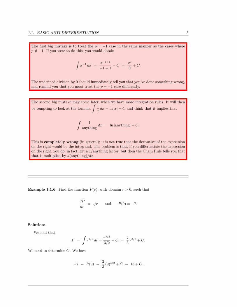
The first big mistake is to treat the p = −1 case in the same manner as the cases wherep 6= −1. If you were to do this, you would obtain
∫x−1 dx =
x−1+1
−1 + 1+ C =
x0
0+ C.
The undefined division by 0 should immediately tell you that you’ve done something wrong,and remind you that you must treat the p = −1 case differently.
The second big mistake may come later, when we have more integration rules. It will then
be tempting to look at the formula∫
1xdx = ln |x|+ C and think that it implies that
∫1
anythingdx = ln |anything|+ C.
This is completely wrong (in general); it is not true that the derivative of the expressionon the right would be the integrand. The problem is that, if you differentiate the expressionon the right, you do, in fact, get a 1/anything factor, but then the Chain Rule tells you thatthat is multiplied by d(anything)/dx.
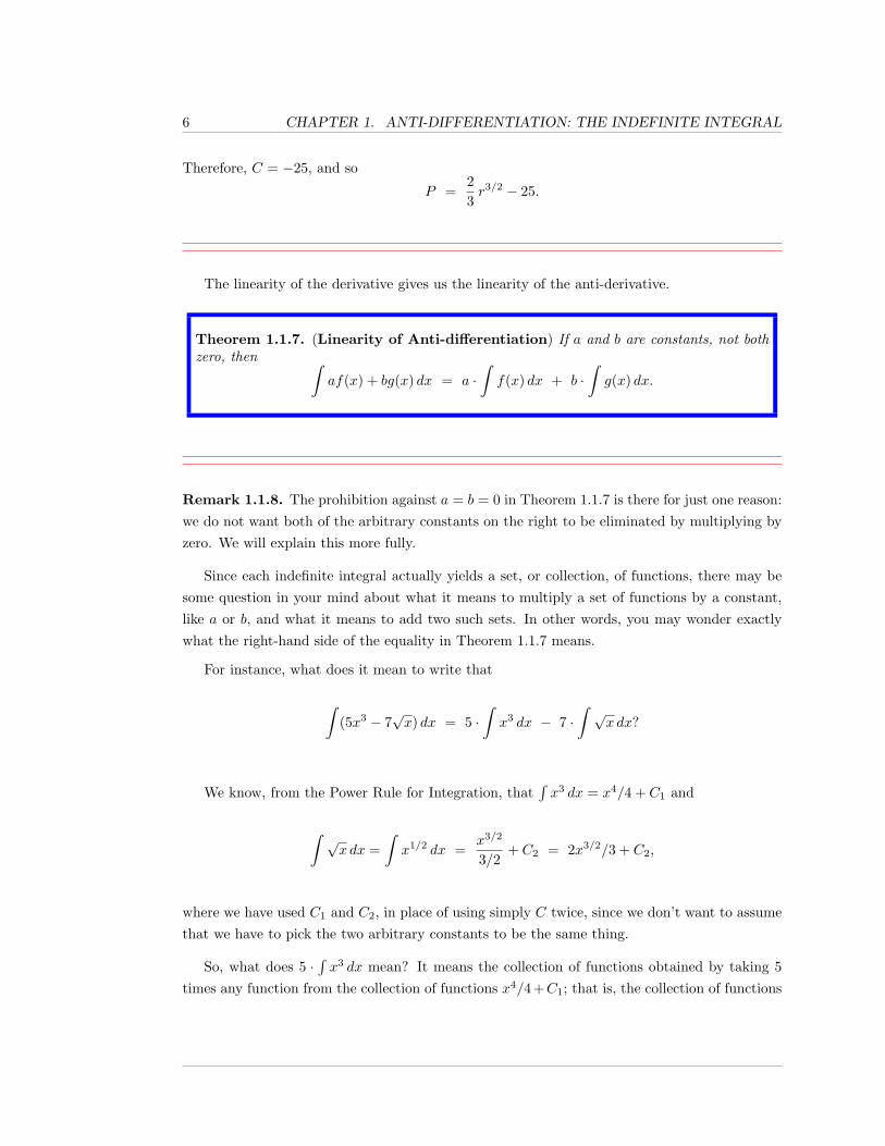
Example 1.1.6. Find the function P (r), with domain r > 0, such that
dP
dr=√r and P (9) = −7.
Solution:
We find that
P =∫r1/2 dr =
r3/2
3/2+ C =
23r3/2 + C.
We need to determine C. We have
−7 = P (9) =23
(9)3/2 + C = 18 + C.
6 CHAPTER 1. ANTI-DIFFERENTIATION: THE INDEFINITE INTEGRAL
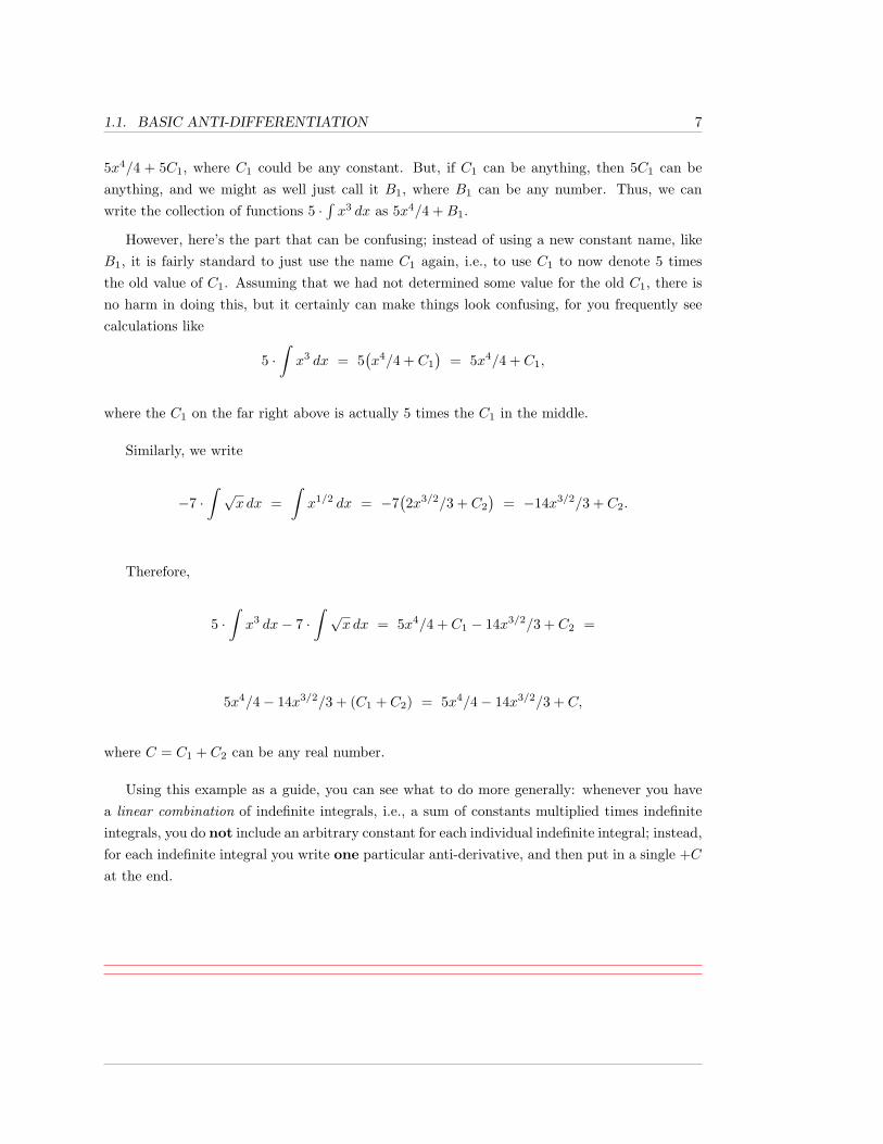
Therefore, C = −25, and so
P =23r3/2 − 25.
The linearity of the derivative gives us the linearity of the anti-derivative.
Theorem 1.1.7. (Linearity of Anti-differentiation) If a and b are constants, not bothzero, then ∫
af(x) + bg(x) dx = a ·∫f(x) dx + b ·
∫g(x) dx.
Remark 1.1.8. The prohibition against a = b = 0 in Theorem 1.1.7 is there for just one reason:we do not want both of the arbitrary constants on the right to be eliminated by multiplying byzero. We will explain this more fully.
Since each indefinite integral actually yields a set, or collection, of functions, there may besome question in your mind about what it means to multiply a set of functions by a constant,like a or b, and what it means to add two such sets. In other words, you may wonder exactlywhat the right-hand side of the equality in Theorem 1.1.7 means.
For instance, what does it mean to write that
∫(5x3 − 7
√x) dx = 5 ·
∫x3 dx − 7 ·
∫ √x dx?
We know, from the Power Rule for Integration, that∫x3 dx = x4/4 + C1 and
∫ √x dx =
∫x1/2 dx =
x3/2
3/2+ C2 = 2x3/2/3 + C2,
where we have used C1 and C2, in place of using simply C twice, since we don’t want to assumethat we have to pick the two arbitrary constants to be the same thing.
So, what does 5 ·∫x3 dx mean? It means the collection of functions obtained by taking 5
times any function from the collection of functions x4/4 +C1; that is, the collection of functions
1.1. BASIC ANTI-DIFFERENTIATION 7
5x4/4 + 5C1, where C1 could be any constant. But, if C1 can be anything, then 5C1 can beanything, and we might as well just call it B1, where B1 can be any number. Thus, we canwrite the collection of functions 5 ·
∫x3 dx as 5x4/4 +B1.
However, here’s the part that can be confusing; instead of using a new constant name, likeB1, it is fairly standard to just use the name C1 again, i.e., to use C1 to now denote 5 timesthe old value of C1. Assuming that we had not determined some value for the old C1, there isno harm in doing this, but it certainly can make things look confusing, for you frequently seecalculations like
5 ·∫x3 dx = 5
(x4/4 + C1
)= 5x4/4 + C1,
where the C1 on the far right above is actually 5 times the C1 in the middle.
Similarly, we write
−7 ·∫ √
x dx =∫x1/2 dx = −7
(2x3/2/3 + C2
)= −14x3/2/3 + C2.
Therefore,
5 ·∫x3 dx− 7 ·
∫ √x dx = 5x4/4 + C1 − 14x3/2/3 + C2 =
5x4/4− 14x3/2/3 + (C1 + C2) = 5x4/4− 14x3/2/3 + C,
where C = C1 + C2 can be any real number.
Using this example as a guide, you can see what to do more generally: whenever you havea linear combination of indefinite integrals, i.e., a sum of constants multiplied times indefiniteintegrals, you do not include an arbitrary constant for each individual indefinite integral; instead,for each indefinite integral you write one particular anti-derivative, and then put in a single +Cat the end.
8 CHAPTER 1. ANTI-DIFFERENTIATION: THE INDEFINITE INTEGRAL
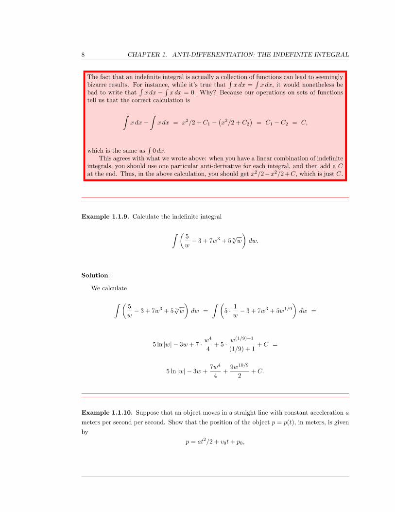
The fact that an indefinite integral is actually a collection of functions can lead to seeminglybizarre results. For instance, while it’s true that
∫x dx =
∫x dx, it would nonetheless be
bad to write that∫x dx −
∫x dx = 0. Why? Because our operations on sets of functions
tell us that the correct calculation is
∫x dx−
∫x dx = x2/2 + C1 −
(x2/2 + C2
)= C1 − C2 = C,
which is the same as∫
0 dx.This agrees with what we wrote above: when you have a linear combination of indefinite
integrals, you should use one particular anti-derivative for each integral, and then add a Cat the end. Thus, in the above calculation, you should get x2/2−x2/2 +C, which is just C.
Example 1.1.9. Calculate the indefinite integral
∫ (5w− 3 + 7w3 + 5 9
√w
)dw.
Solution:
We calculate
∫ (5w− 3 + 7w3 + 5 9
√w
)dw =
∫ (5 · 1
w− 3 + 7w3 + 5w1/9
)dw =
5 ln |w| − 3w + 7 · w4
4+ 5 · w
(1/9)+1
(1/9) + 1+ C =
5 ln |w| − 3w +7w4
4+
9w10/9
2+ C.
Example 1.1.10. Suppose that an object moves in a straight line with constant acceleration ameters per second per second. Show that the position of the object p = p(t), in meters, is givenby
p = at2/2 + v0t+ p0,
1.1. BASIC ANTI-DIFFERENTIATION 9
where p0 is the initial position of the object (i.e., the position at t = 0), in meters, v0 is theinitial velocity in m/s, and t is the time in seconds.
Solution:
Acceleration a is the derivative, with respect to t, of the velocity v, i.e., a = dv/dt. This isexactly the same as writing that v is an anti-derivative of a, with respect to t, i.e., v =
∫a dt.
Since a is a constant, we find
v =∫a dt = a
∫1 dt = at+ C m/s,
for some constant C. Therefore, v = at + C, but we would like to give some physical meaningto the constant C.
How do we do this? We are not given any other data. The answer is that we use tautologicalinitial data; that is, we use initial data that is simply obviously true. We use that, when t = 0,the velocity v equals v0. Why is this true? Because it says something that’s clearly true: at time0, the velocity equals the velocity at time 0. It may seem strange, but using this tautologicalinitial data actually gets us somewhere.
We have v = at + C. Now, plug in that, when t = 0, v = v0. You find v0 = a · 0 + C, i.e.,C = v0. Thus, we conclude that v = at+ v0. Notice that no one has to give you any extra datato conclude that C = v0; it follows from the equation v = at+ C.
Now, we have that v = at+ v0, and we know that the velocity v equals the rate of change ofp, with respect to time, i.e., v = dp/dt. This is the same as writing that p =
∫v dt. Therefore,
we havep =
∫v dt =
∫(at+ v0) dt = a
(∫t dt
)+ v0
(∫1 dt)
=
at2/2 + v0t+ C meters,
where this C is definitely not the same C that we used in the equation for v.
How do we find this new C? We plug in more tautological initial data, namely that p = p0
when t = 0. We find that p0 = a(0)2/2 + v0(0) + C, and so C = p0. Thus, we conclude
p = at2/2 + v0t+ p0 meters.
Other integration formulas obtained at once from differentiation formulas are:
10 CHAPTER 1. ANTI-DIFFERENTIATION: THE INDEFINITE INTEGRAL
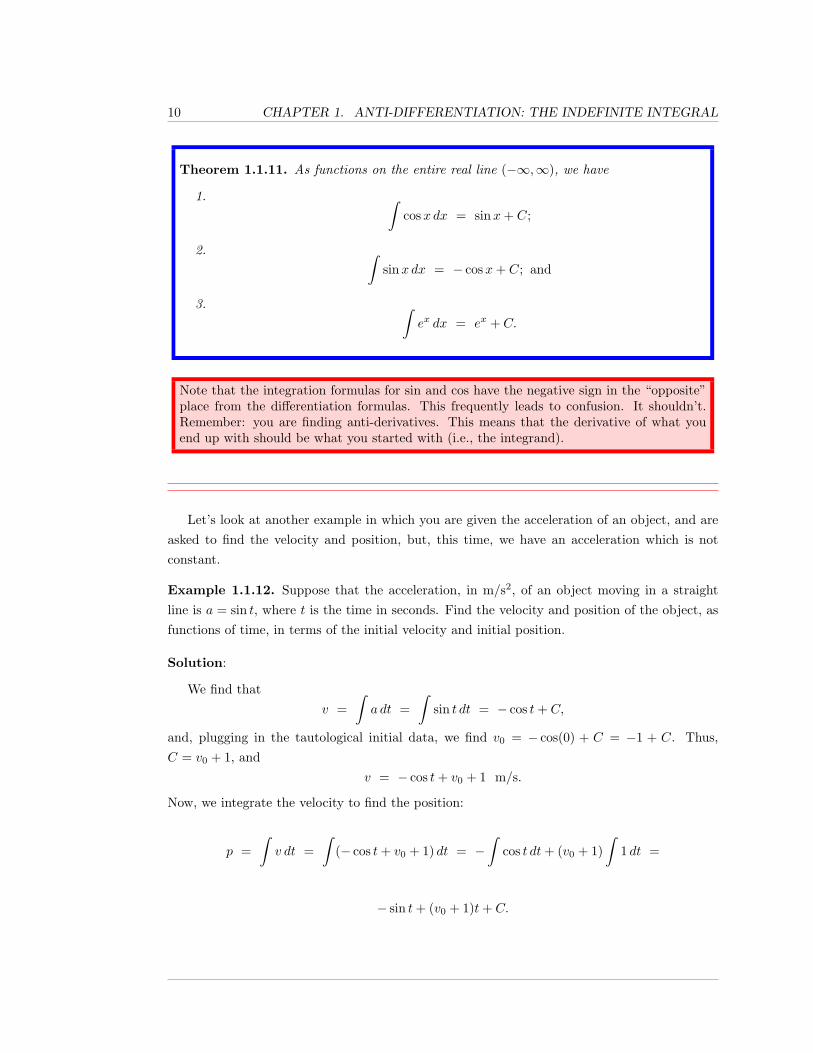
Theorem 1.1.11. As functions on the entire real line (−∞,∞), we have
1. ∫cosx dx = sinx+ C;
2. ∫sinx dx = − cosx+ C; and
3. ∫ex dx = ex + C.
Note that the integration formulas for sin and cos have the negative sign in the “opposite”place from the differentiation formulas. This frequently leads to confusion. It shouldn’t.Remember: you are finding anti-derivatives. This means that the derivative of what youend up with should be what you started with (i.e., the integrand).
Let’s look at another example in which you are given the acceleration of an object, and areasked to find the velocity and position, but, this time, we have an acceleration which is notconstant.
Example 1.1.12. Suppose that the acceleration, in m/s2, of an object moving in a straightline is a = sin t, where t is the time in seconds. Find the velocity and position of the object, asfunctions of time, in terms of the initial velocity and initial position.
Solution:
We find thatv =
∫a dt =
∫sin t dt = − cos t+ C,
and, plugging in the tautological initial data, we find v0 = − cos(0) + C = −1 + C. Thus,C = v0 + 1, and
v = − cos t+ v0 + 1 m/s.
Now, we integrate the velocity to find the position:
p =∫v dt =
∫(− cos t+ v0 + 1) dt = −
∫cos t dt+ (v0 + 1)
∫1 dt =
− sin t+ (v0 + 1)t+ C.
1.1. BASIC ANTI-DIFFERENTIATION 11
Finally, we plug in the tautological initial data, in order to give physical meaning to this lastC:
p0 = − sin(0) + (v0 + 1)(0) + C.
Therefore, C = p0, and we find
p = − sin t+ (v0 + 1)t+ p0 meters.
We shall not rewrite, as anti-differentiation formulas, every one of the differentiation formulasthat you should know; the standard anti-differentiation formulas are contained in Appendix B.However, we’ll go ahead and give two more, before looking at the Chain Rule and the ProductRule in their indefinite integral forms.
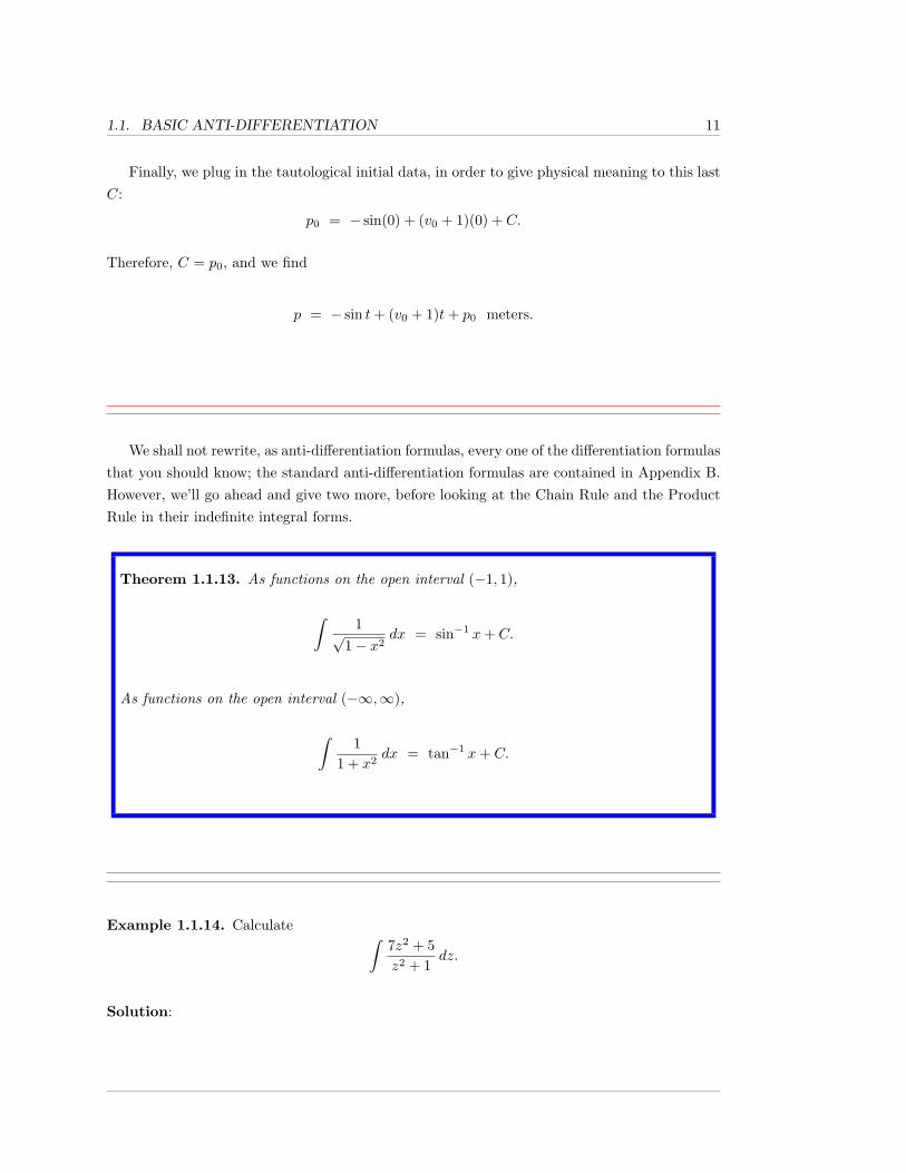
Theorem 1.1.13. As functions on the open interval (−1, 1),
∫1√
1− x2dx = sin−1 x+ C.
As functions on the open interval (−∞,∞),
∫1
1 + x2dx = tan−1 x+ C.
Example 1.1.14. Calculate ∫7z2 + 5z2 + 1
dz.
Solution:
12 CHAPTER 1. ANTI-DIFFERENTIATION: THE INDEFINITE INTEGRAL
We begin by “simplifying” via long division of polynomials, except the division is not so longin this case. We get clever and write 7z2 = 7(z2 + 1)− 7, and find
7z2 + 5z2 + 1
=7(z2 + 1)− 7 + 5
z2 + 1= 7− 2 · 1
z2 + 1.
Thus,
∫7z2 + 5z2 + 1
dz =∫ (
7− 2 · 1z2 + 1
)dz = 7
∫1 dz − 2 ·
∫1
z2 + 1dz =
7z − 2 tan−1 z + C.
Substitution: the Chain Rule in anti-derivative form:
The Chain Rule for differentiation tells you how to differentiate a composition of functions.If f and g are differentiable, then
(f(g(x))
)′ = f ′(g(x))g′(x) or, letting u = g(x), the ChainRule can be written as
d
dx
(f(u)
)= f ′(u)
du
dx.
As an anti-derivative formula, this becomes
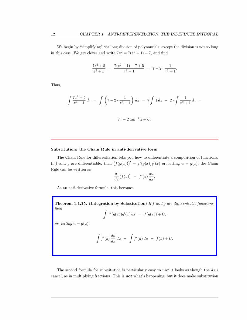
Theorem 1.1.15. (Integration by Substitution) If f and g are differentiable functions,then ∫
f ′(g(x))g′(x) dx = f(g(x)) + C,
or, letting u = g(x),
∫f ′(u)
du
dxdx =
∫f ′(u) du = f(u) + C.
The second formula for substitution is particularly easy to use; it looks as though the dx’scancel, as in multiplying fractions. This is not what’s happening, but it does make substitution
1.1. BASIC ANTI-DIFFERENTIATION 13
easier to remember. It also means that the differential notation
du =du
dxdx,
which we introduced in [2], yields correct formulas in integrals, and, hence, we use it extensively.
Example 1.1.16. Calculate the integral
∫cos(ex + 7) · ex dx.
Solution:
How should you approach an integral like
∫cos(ex + 7) · ex dx?
First, you should realize that it’s not just a linear combination of integrals of specific functionsthat you’ve memorized. You should then think “Well...cos(ex+ 7) is a composition of functions.What if I make a substitution for the “inside” function? I’ll let u = ex + 7, so that cos(ex + 7)becomes cosu, and see if the remaining part of the integrand looks like du.”
In fact, for easy cases, you can do this in your head. If u = ex + 7, then
du =du
dxdx = ex dx,
and you see that this is the remaining “factor” in the integral. Thus, by substitution, our originalintegral is transformed into an integral in terms of u that is very simple:
∫cos(ex + 7) · ex dx =
∫cosu du = sinu+ C = sin(ex + 7) + C.
Nice.
14 CHAPTER 1. ANTI-DIFFERENTIATION: THE INDEFINITE INTEGRAL
Example 1.1.17. Calculate the integral
∫t
1 + t2dt.
Solution:
You once again realize that this integral is not some linear combination of basic integralsthat have memorized, and there’s no obvious composition of functions this time. You mightthink that tan−1 t is involved somehow, since
∫1/(1 + t2) dt = tan−1 t + C, but the t in the
numerator causes a problem.
You might think that you can factor the integrand and use that in some way:
∫t
1 + t2dt =
∫t · 1
1 + t2dt
?=?
∫t dt ·
∫1
1 + t2dt =
t2
2· tan−1 t+ C.
THIS IS COMPLETELY WRONG. You can’t just integrate each factor in a productand then multiply the results; dealing with products in an integral is more complicated thanthat.
We will get to the integral form of the Product Rule shortly, but, for now, you shoulddifferentiate t2 tan−1 t/2 (using the Product Rule) and verify that you don’t get anything closeto our integrand t/(1 + t2).
Great. Now we know one way NOT to find the integral∫t/(1 + t2) dt. We also know that
we’re discussing substitution here, and so you should suspect that a substitution is involved.
With practice, you should actually see relatively quickly that if you let w = 1 + t2, thendw = 2t dt, and we have a t dt in the integral, so this substitution might be good. We canalways “fix” multiplying by a constant, like the 2 in dw = 2t dt. We divide by 2 to get
12dw = t dt,
and ∫t
1 + t2dt =
∫1
1 + t2· t dt =
∫1w· 1
2dw =
1.1. BASIC ANTI-DIFFERENTIATION 15
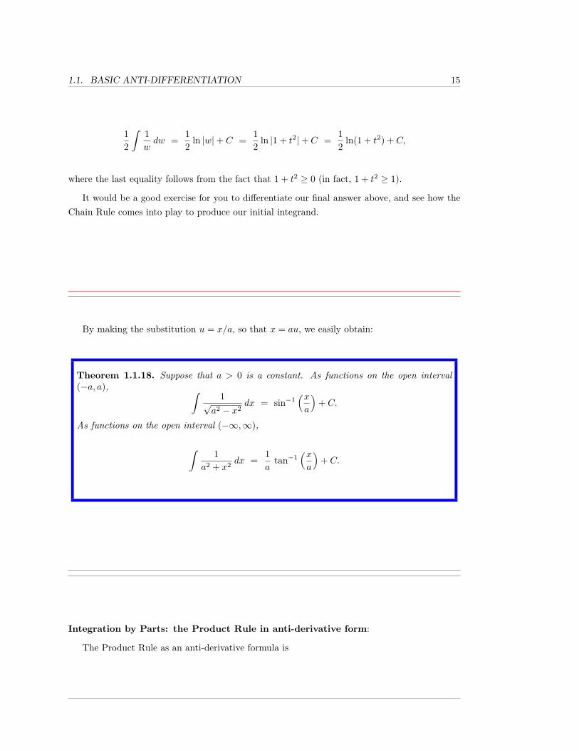
12
∫1wdw =
12
ln |w|+ C =12
ln |1 + t2|+ C =12
ln(1 + t2) + C,
where the last equality follows from the fact that 1 + t2 ≥ 0 (in fact, 1 + t2 ≥ 1).
It would be a good exercise for you to differentiate our final answer above, and see how theChain Rule comes into play to produce our initial integrand.
By making the substitution u = x/a, so that x = au, we easily obtain:
Theorem 1.1.18. Suppose that a > 0 is a constant. As functions on the open interval(−a, a), ∫
1√a2 − x2
dx = sin−1(xa
)+ C.
As functions on the open interval (−∞,∞),
∫1
a2 + x2dx =
1a
tan−1(xa
)+ C.
Integration by Parts: the Product Rule in anti-derivative form:
The Product Rule as an anti-derivative formula is
16 CHAPTER 1. ANTI-DIFFERENTIATION: THE INDEFINITE INTEGRAL
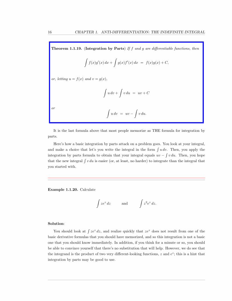
Theorem 1.1.19. (Integration by Parts) If f and g are differentiable functions, then
∫f(x)g′(x) dx+
∫g(x)f ′(x) dx = f(x)g(x) + C,
or, letting u = f(x) and v = g(x),
∫u dv +
∫v du = uv + C
or ∫u dv = uv −
∫v du.
It is the last formula above that most people memorize as THE formula for integration byparts.
Here’s how a basic integration by parts attack on a problem goes. You look at your integral,and make a choice that let’s you write the integral in the form
∫u dv. Then, you apply the
integration by parts formula to obtain that your integral equals uv −∫v du. Then, you hope
that the new integral∫v du is easier (or, at least, no harder) to integrate than the integral that
you started with.
Example 1.1.20. Calculate
∫zez dz and
∫z2ez dz.
Solution:
You should look at∫zez dz, and realize quickly that zez does not result from one of the
basic derivative formulas that you should have memorized, and so this integration is not a basicone that you should know immediately. In addition, if you think for a minute or so, you shouldbe able to convince yourself that there’s no substitution that will help. However, we do see thatthe integrand is the product of two very different-looking functions, z and ez; this is a hint thatintegration by parts may be good to use.
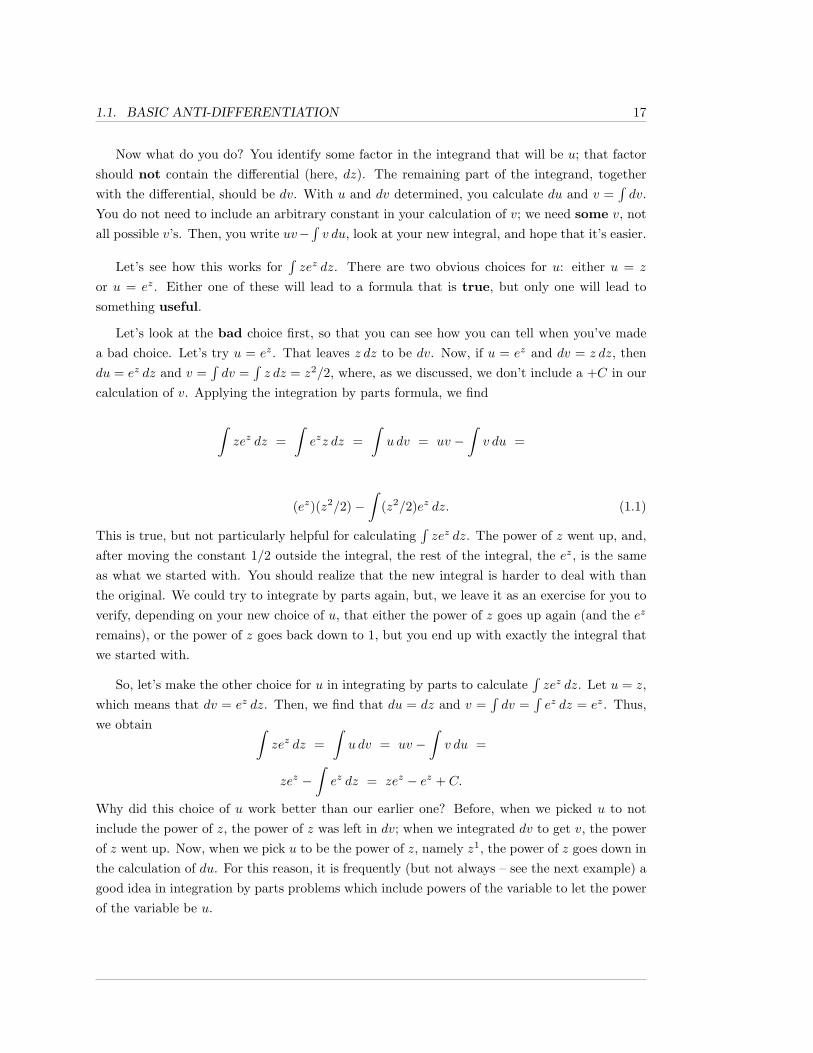
1.1. BASIC ANTI-DIFFERENTIATION 17
Now what do you do? You identify some factor in the integrand that will be u; that factorshould not contain the differential (here, dz). The remaining part of the integrand, togetherwith the differential, should be dv. With u and dv determined, you calculate du and v =
∫dv.
You do not need to include an arbitrary constant in your calculation of v; we need some v, notall possible v’s. Then, you write uv−
∫v du, look at your new integral, and hope that it’s easier.
Let’s see how this works for∫zez dz. There are two obvious choices for u: either u = z
or u = ez. Either one of these will lead to a formula that is true, but only one will lead tosomething useful.
Let’s look at the bad choice first, so that you can see how you can tell when you’ve madea bad choice. Let’s try u = ez. That leaves z dz to be dv. Now, if u = ez and dv = z dz, thendu = ez dz and v =
∫dv =
∫z dz = z2/2, where, as we discussed, we don’t include a +C in our
calculation of v. Applying the integration by parts formula, we find
∫zez dz =
∫ezz dz =
∫u dv = uv −
∫v du =
(ez)(z2/2)−∫
(z2/2)ez dz. (1.1)
This is true, but not particularly helpful for calculating∫zez dz. The power of z went up, and,
after moving the constant 1/2 outside the integral, the rest of the integral, the ez, is the sameas what we started with. You should realize that the new integral is harder to deal with thanthe original. We could try to integrate by parts again, but, we leave it as an exercise for you toverify, depending on your new choice of u, that either the power of z goes up again (and the ez
remains), or the power of z goes back down to 1, but you end up with exactly the integral thatwe started with.
So, let’s make the other choice for u in integrating by parts to calculate∫zez dz. Let u = z,
which means that dv = ez dz. Then, we find that du = dz and v =∫dv =
∫ez dz = ez. Thus,
we obtain ∫zez dz =
∫u dv = uv −
∫v du =
zez −∫ez dz = zez − ez + C.
Why did this choice of u work better than our earlier one? Before, when we picked u to notinclude the power of z, the power of z was left in dv; when we integrated dv to get v, the powerof z went up. Now, when we pick u to be the power of z, namely z1, the power of z goes down inthe calculation of du. For this reason, it is frequently (but not always – see the next example) agood idea in integration by parts problems which include powers of the variable to let the powerof the variable be u.
18 CHAPTER 1. ANTI-DIFFERENTIATION: THE INDEFINITE INTEGRAL
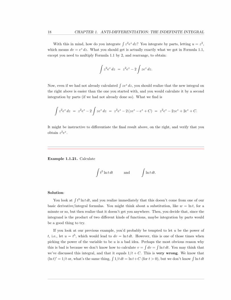
With this in mind, how do you integrate∫z2ez dz? You integrate by parts, letting u = z2,
which means dv = ez dz. What you should get is actually exactly what we got in Formula 1.1,except you need to multiply Formula 1.1 by 2, and rearrange, to obtain:
∫z2ez dz = z2ez − 2
∫zez dz.
Now, even if we had not already calculated∫zez dz, you should realize that the new integral on
the right above is easier than the one you started with, and you would calculate it by a secondintegration by parts (if we had not already done so). What we find is
∫z2ez dz = z2ez − 2
∫zez dz = z2ez − 2 (zez − ez + C) = z2ez − 2zez + 2ez + C.
It might be instructive to differentiate the final result above, on the right, and verify that youobtain z2ez.
Example 1.1.21. Calculate
∫t5 ln t dt and
∫ln t dt.
Solution:
You look at∫t5 ln t dt, and you realize immediately that this doesn’t come from one of our
basic derivative/integral formulas. You might think about a substitution, like w = ln t, for aminute or so, but then realize that it doesn’t get you anywhere. Then, you decide that, since theintegrand is the product of two different kinds of functions, maybe integration by parts wouldbe a good thing to try.
If you look at our previous example, you’d probably be tempted to let u be the power oft, i.e., let u = t5, which would lead to dv = ln t dt. However, this is one of those times whenpicking the power of the variable to be u is a bad idea. Perhaps the most obvious reason whythis is bad is because we don’t know how to calculate v =
∫dv =
∫ln t dt. You may think that
we’ve discussed this integral, and that it equals 1/t + C. This is very wrong. We know that(ln t)′ = 1/t or, what’s the same thing,
∫1/t dt = ln t+C (for t > 0), but we don’t know
∫ln t dt
1.1. BASIC ANTI-DIFFERENTIATION 19
(it’s possible that you do, but it hasn’t been discussed in the book up to this point). In fact,calculating
∫ln t dt is the second part of this example.
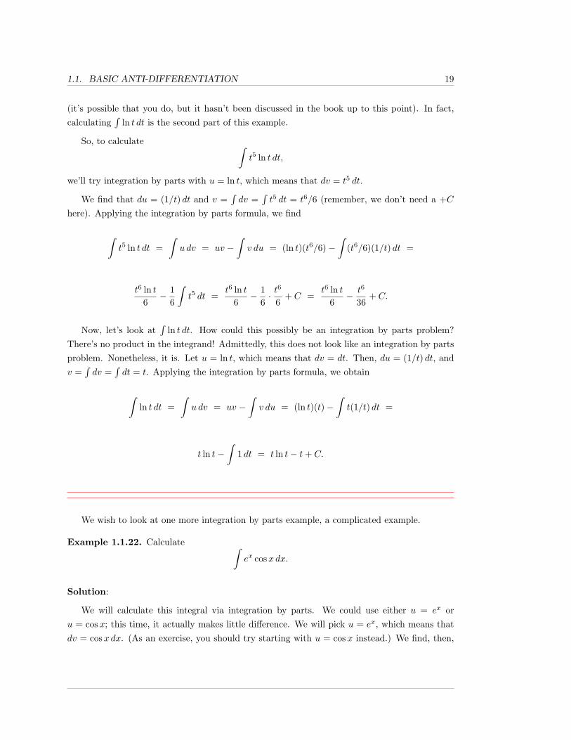
So, to calculate ∫t5 ln t dt,
we’ll try integration by parts with u = ln t, which means that dv = t5 dt.
We find that du = (1/t) dt and v =∫dv =
∫t5 dt = t6/6 (remember, we don’t need a +C
here). Applying the integration by parts formula, we find
∫t5 ln t dt =
∫u dv = uv −
∫v du = (ln t)(t6/6)−
∫(t6/6)(1/t) dt =
t6 ln t6− 1
6
∫t5 dt =
t6 ln t6− 1
6· t
6
6+ C =
t6 ln t6− t6
36+ C.
Now, let’s look at∫
ln t dt. How could this possibly be an integration by parts problem?There’s no product in the integrand! Admittedly, this does not look like an integration by partsproblem. Nonetheless, it is. Let u = ln t, which means that dv = dt. Then, du = (1/t) dt, andv =
∫dv =
∫dt = t. Applying the integration by parts formula, we obtain
∫ln t dt =
∫u dv = uv −
∫v du = (ln t)(t)−
∫t(1/t) dt =
t ln t−∫
1 dt = t ln t− t+ C.
We wish to look at one more integration by parts example, a complicated example.
Example 1.1.22. Calculate ∫ex cosx dx.
Solution:
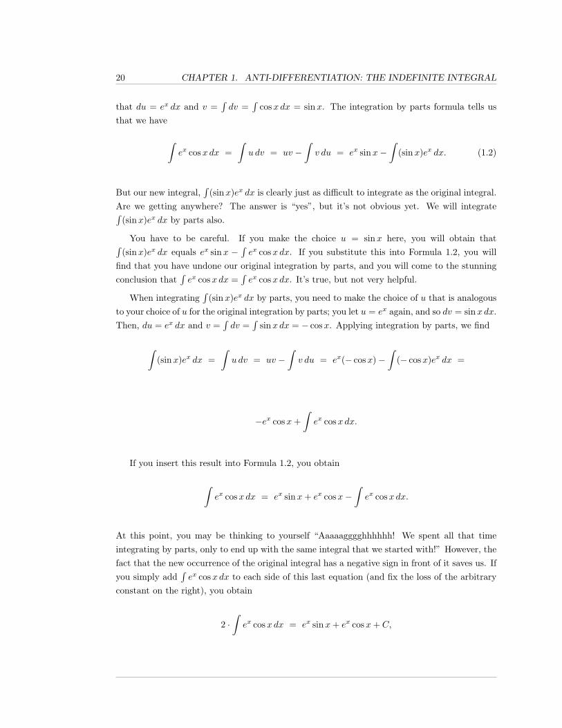
We will calculate this integral via integration by parts. We could use either u = ex oru = cosx; this time, it actually makes little difference. We will pick u = ex, which means thatdv = cosx dx. (As an exercise, you should try starting with u = cosx instead.) We find, then,
20 CHAPTER 1. ANTI-DIFFERENTIATION: THE INDEFINITE INTEGRAL
that du = ex dx and v =∫dv =
∫cosx dx = sinx. The integration by parts formula tells us
that we have
∫ex cosx dx =
∫u dv = uv −
∫v du = ex sinx−
∫(sinx)ex dx. (1.2)
But our new integral,∫
(sinx)ex dx is clearly just as difficult to integrate as the original integral.Are we getting anywhere? The answer is “yes”, but it’s not obvious yet. We will integrate∫
(sinx)ex dx by parts also.
You have to be careful. If you make the choice u = sinx here, you will obtain that∫(sinx)ex dx equals ex sinx −
∫ex cosx dx. If you substitute this into Formula 1.2, you will
find that you have undone our original integration by parts, and you will come to the stunningconclusion that
∫ex cosx dx =
∫ex cosx dx. It’s true, but not very helpful.
When integrating∫
(sinx)ex dx by parts, you need to make the choice of u that is analogousto your choice of u for the original integration by parts; you let u = ex again, and so dv = sinx dx.Then, du = ex dx and v =
∫dv =
∫sinx dx = − cosx. Applying integration by parts, we find
∫(sinx)ex dx =
∫u dv = uv −
∫v du = ex(− cosx)−
∫(− cosx)ex dx =
−ex cosx+∫ex cosx dx.
If you insert this result into Formula 1.2, you obtain
∫ex cosx dx = ex sinx+ ex cosx−
∫ex cosx dx.
At this point, you may be thinking to yourself “Aaaaagggghhhhhh! We spent all that timeintegrating by parts, only to end up with the same integral that we started with!” However, thefact that the new occurrence of the original integral has a negative sign in front of it saves us. Ifyou simply add
∫ex cosx dx to each side of this last equation (and fix the loss of the arbitrary
constant on the right), you obtain
2 ·∫ex cosx dx = ex sinx+ ex cosx+ C,
1.1. BASIC ANTI-DIFFERENTIATION 21
and so ∫ex cosx dx =
ex sinx+ ex cosx2
+ C.
We end this section with a possibly surprising complication that exists for anti-differentiation;a type of complication which does not occur for differentiation.
Remark 1.1.23. From the derivative formulas in [2], we see that the derivative of any elemen-tary function is again an elementary function. You might hope that anti-derivatives/integralswould behave equally as well. They do not. It is easy to give elementary functions f(x) forwhich it is possible to prove that there is no elementary function F (x) such that F ′(x) = f(x),i.e., f(x) has no elementary anti-derivative. Such functions f(x) include ex
2, e−x
2, sin(x2), and
cos(x2). This was first proved by Liouville in 1835.
The Fundamental Theorem of Calculus, Theorem 2.4.7, guarantees that the functions ex2,
e−x2, sin(x2), and cos(x2), and, in fact, all continuous functions, have some anti-derivative, but
those anti-derivatives need not be elementary functions.
1.1.1 Exercises
Calculate the general anti-derivatives in Exercises 1 through 21.
1.∫
(4x2 + 4x+ 9) dx
2.∫ (
5w− 7ew + 6 3
√w
)dw
3.∫ (
5 sin t− 3√1− t2
)dt
4.∫
1 + v +√v
v2dv
5.∫ (
1y
+1
y2 + 1
)dy
6.∫
53z − 7
dz
7.∫
cos(2θ − 1) dθ
22 CHAPTER 1. ANTI-DIFFERENTIATION: THE INDEFINITE INTEGRAL
8.∫ep+4 dp
9.∫
r
r2 − 4dr
10.∫ (
x√x2 − 1
+1
|x|√x2 − 1
)dx
11.∫
(5ω − 3)100 dω
12.∫ (
2 cos(2t+ 5) + 3 sin(9t))dt
13.∫
ln[(x+ 2)x+5
]dx
14.∫e1/x
x3dx
15.∫
5x lnx
dx
16.∫e1/x
6x2dx
17.∫
tan θ dθ
18.∫
54 + x2
dx
19.∫t4√t5 + 6 dt
20.∫
1x2 + 4x+ 5
dx Hint: x2 + 4x+ 5 = (x+ 2)2 + 1.
21.∫
1√−x2 + 6x− 8
dx
In each of Exercises 22 through 31, find the anti-derivative of the given function
which satisfies the given initial condition. The anti-derivative of each function with
a lower-case name is denoted by the upper-case version of the same letter.
22. h(x) = 4x2 + 4x+ 9, such that H(−1) = 2.
23. p(w) =5w− 7ew + 6 3
√w, such that P (−1) = 0.
24. q(t) = 5 sin t− 3√1− t2
, such that Q(0) = 7.
1.1. BASIC ANTI-DIFFERENTIATION 23
25. k(v) =1 + v +
√v
v2, such that K(1) = −2.
26. b(y) =1y
+1
y2 + 1, such that B(1) = 0.
27. f(x) = x2 + x sinx, such that F (π) = 2π.
28. s(t) =2
t(ln t)2, such that S(e2) = 5.
29. g(x) = x√x+ 1, such that G(0) = 1.
30. w(y) =tan−1
(y2
)4 + y2
, such that W (2) = π.
31. r(t) = te1−t2 − t, such that R(1) =√
2.
In each of Exercises 32 through 41, use integration by parts to find the indicated
anti-derivative.
32.∫xe3x dx
33.∫
(x− 5)2ex dx
34.∫t sin(2t) dt
35.∫t2 cos t dt
36.∫ √
p ln p dp
37.∫
ln tt2
dt
38.∫ex sinx dx
39.∫e2x sin(5x) dx
40.∫
tan−1 w dw
41.∫w tan−1 w dw Hint: At some point, you may want to use that w2 = (1 + w2)− 1.
42. Suppose that the net force F , acting on an object of mass m, pushes the object along thex-axis with an acceleration function, in m/s2, of
a(t) = sin(2t),
where t ≥ 0 is measured in seconds.
24 CHAPTER 1. ANTI-DIFFERENTIATION: THE INDEFINITE INTEGRAL
a. Recall that F = ma and that momentum p = mv. Find the momentum of the object,as a function of time, if the mass of the object is 10 kilograms, and momentum attime t = 0 is 20 kilogram meters per second.
b. What is the momentum of the object at time t = 4 seconds?
43. Repeat the preceding problem with the new acceleration function a(t) = t · sin(2t).
44. For each positive integer n, define fn(θ) = sinn θ cos θ and gn(θ) = cosn θ sin θ
a. Find∫fn(θ) dθ and
∫gn(θ) dθ.
b. Find the specific anti-derivatives Fn(θ) and Gn(θ) that satisfy the initial conditionsFn(0) = 5 and Gn
(π2
)= 4.
In Exercises 45 through 48, you are given the velocity of a particle at time t, and
the position p(t0) of the particle at a specific time t0. Find the position function.
45. v(t) = 3t2 − 4t+ 3, p(1) = 4.
46. v(t) = t+ cos(t), p(0) = 0.
47. v(t) = 2t√
18 + 7t2, p(1) = 8.
48. v(t) = at+ b, p(2) = 5. Leave your answer in terms of a and b.
49. In the following steps, you will calculate the general anti-derivatives for sin2 x and cos2 x.
a. Apply integration by parts to∫
sinx · sinx dx (written suggestively).
b. Integration by parts yields a new anti-derivative. Use a trigonometric identity towrite this new anti-derivative in terms of sin2 x, and solve your integration by parts
equation for∫
sin2 x dx.
c. What is∫
cos2 x dx? Hint: Use your answer to part (b).
d. From the cosine double angle formula, cos(2x) = 2 cos2 x − 1. Use this to integratecos2 x, and explain why the different-looking answer that you obtain is, in fact, thesame as your answer from part (c).
Exercises 50 and 51 show that the argument in Exercise 49 can be generalized to
calculate anti-derivatives of higher powers of sin and cos.
1.1. BASIC ANTI-DIFFERENTIATION 25
50. a. Use integration by parts to prove that
∫sinn t dt = − 1
ncos t sinn−1 t+
n− 1n
∫sinn−2 t dt.
Assume n ≥ 2.
b. Use this formula to calculate∫
sin2 t dt. Check your answer by comparing to the
previous problem.
51. a. Use integration by parts to prove that
∫cosn t dt =
1n
cosn−1 t sin t+n− 1n
∫cosn−2 t dt.
b. Use the formula in part (a) to determine∫
cos2 t dt.
52. Suppose that instantaneous rate of change, with respect to time, of a population of anisland at time t, measured in years, where t = 0 corresponds to the year 2000, is given by
12√
6, 250, 000 + t− 500
(t+ 1)2.
The population of the island in 2000 is 3000.
a. Find an explicit formula for the population at time t.
b. What is the predicted population in 2050?
53. Prove that the argument used to calculate∫
ln t dt can be generalized. Assume that f(t)
is differentiable and prove that
∫f(t) dt = tf(t)−
∫tf ′(t) dt.
54. Calculate∫ex sinhx dx. Hint: do not use integration by parts.
26 CHAPTER 1. ANTI-DIFFERENTIATION: THE INDEFINITE INTEGRAL
55. Consider the following logic in calculating∫ex sinhx dx using integration by parts.
∫ex sinhx dx = ex sinhx−
∫ex coshx dx
= ex sinhx−(ex coshx−
∫ex sinhx dx
)⇒
0 = ex sinhx− ex coshx⇒
ex sinhx = ex coshx.
Since ex > 0, we can divide and conclude that sinhx = coshx. What is the flaw in thisargument?
56. Prove the formula ∫tnet dt = tnet − n
∫tn−1et dt.
Assume that n ≥ 1.
57. Calculate∫
1x2 + a2
dx, where a 6= 0 is a constant. Hint: use Theorem 4.2.14 and an
appropriate substitution.
58. Prove that∫
dx√x2 + a2
= sinh−1(xa
)+ C.
59. Calculate∫
1√a2 − x2
dx, where a > 0 is a constant.
60. Calculate∫
1|x|√x2 − 1
dx. Hint: consider sec−1 x.
61. Calculate∫exee
x
dx. Hint: use substitution.
62. Let f1(x) = ex and, for all integers n ≥ 2, let fn(x) = efn−1(x). Prove that
∫f1(x) · f2(x) · ... · fn(x) dx = fn(x) + C.
63. Calculate∫
2x dx. Hint: rewrite 2x as an exponential expression with base e.
64. Calculate∫
x+ 4√x+ 2
dx.
65. Calculate∫
ln(1 + x2) dx.
1.1. BASIC ANTI-DIFFERENTIATION 27
66. Calculate∫e3x − e2x
e2x − 1dx.
Consider a simple electric circuit with an inductor, but no resistor or capacitor.
A battery supplies voltage V (t). If inductance is constantly L, in henrys, then
Kirchoff’s Law from Example 2.7.18 of [2] tells us that the current i at time t
satisfies the differential equation Ldi
dt= V (t). In Exercises 67 through 70, find an
explicit formula for i(t), given the condition i(t0) = i0.
67. L = 12, V (t) = sin t, i(0) = 0.
68. L = 9, V (t) = 12, i(3) = 12.
69. L = 3, V (t) =t
t2 + 1, i(0) = 0.
70. L = 13, V (t) =ln(1/t)t2
, i(1) = 2.
For each of the functions in Exercises 71 through 74, verify that (a)d
dx
[∫f(x) dx
]=
f(x) and (b)∫ [
d
dxf(x)
]dx = f(x) + C. Assume an appropriate domain for f(x).
71. f(x) = x4.
72. f(x) = 3 cos(2x).
73. f(x) = lnx.
74. f(x) =1
1 + x2.
75. In the following steps, you will find the general anti-derivatives for functions of the form
tn ln t.
a. Suppose that n 6= −1. Apply integration by parts to find∫tn ln t dt.
b. Find∫t−1 ln t dt.
76. Suppose that water flows out of a hole 0.1 square meters in area from the bottom of acylindrical tank with a base radius of 2 meters and an initial height of 10 meters at a rate
dV
dt= 0.007798t− 1.3999 cubic meters per second.
28 CHAPTER 1. ANTI-DIFFERENTIATION: THE INDEFINITE INTEGRAL
a. If the tank starts out full, what is the function V (t) for the volume in the tank attime t?
b. Calculate the amount of water remaining in the tank one minute after the leak starts.
c. Verify that dVdt = 0 precisely when the tank is empty.
77. A particle is traveling along the curve y = x2, so that its x-coordinate is a function oftime t, measured in minutes. Suppose that the horizontal velocity (i.e., velocity in onlythe horizontal direction) is given by dx/dt = 0.5 cos3 t miles per minute.
a. What is the maximum horizontal speed (absolute value of velocity) on the time in-terval 0 ≤ t ≤ 20π?
b. Find the function x(t), the x-coordinate of the particle at time t, subject to thecondition that the particle is at the origin at time t = 0.
c. Find the function y(t), the y-coordinate of the particle at time t.
d. What is the vertical velocity of the particle at time t = π minutes?
78. An enclosed room is built in order to experiment with the effects of pressure changes onobjects. Suppose that the equipment is capable of decreasing the pressure in the roomat a rate of − 2
t+1 − 0.04t kilopascals, kPa, per second, and that it can run for up to oneminute before overheating.
a. If the internal pressure in the room is 101.325 kPa (equal to the standard atmosphericpressure or atm), find an expression for P (t).
b. How long will it take to reach 50 kPa (this is approximately the atmospheric pressurefive and a half kilometers above the surface of the Earth)?
c. What is the lowest pressure that can be reached in the room?
In Exercises 79 through 82, you are given the acceleration, a = a(t) in m/s2, of an
object moving in a straight line, where t is the time in seconds. Find the velocity
v and position p of the object, as functions of time, in terms of the initial velocity
v0 and initial position p0.
79. a = t+ 1
80. a = sin t+ cos t
81. a = e−3t
82. a = te−t
1.2. SPECIAL TRIG. INTEGRALS AND TRIG. SUBSTITUTIONS 29
1.2 Special Trigonometric Integralsand Trigonometric Substitutions
In this section, we will discuss some special, important, trigonometric integrals, and then givethree examples of integration by trigonometric substitution.
Proposition 1.2.1.
∫tan θ dθ = − ln | cos θ|+ C = ln | sec θ|+ C.
Proof. We have ∫tan θ dθ =
∫sin θcos θ
dθ.
Let u = cos θ, so that du = − sin θ dθ, i.e., −du = sin θ dθ. We find
∫sin θcos θ
dθ =∫−duu
= − ln |u|+ C = − ln | cos θ|+ C.
Proposition 1.2.2. ∫sec θ dθ = ln | sec θ + tan θ|+ C.
Proof. As (tan θ)′ = sec2 θ and (sec θ)′ = sec θ tan θ, it follows that
(tan θ + sec θ)′ = sec2 θ + sec θ tan θ = (sec θ)(tan θ + sec θ).
This means that, if u = tan θ + sec θ, then du/dθ = u sec θ, i.e.,
∫sec θ dθ =
∫1udu = ln |u|+ C = ln | sec θ + tan θ|+ C.
30 CHAPTER 1. ANTI-DIFFERENTIATION: THE INDEFINITE INTEGRAL
Proposition 1.2.3.
∫sec3 θ dθ =
sec θ tan θ + ln | sec θ + tan θ|2
+ C.
Proof. This is a “fun” integration by parts problem.
∫sec3 θ dθ =
∫sec θ(1 + tan2 θ) dθ =
∫sec θ dθ +
∫sec θ tan2 θ dθ =
ln | sec θ + tan θ| +∫
(tan θ)(sec θ tan θ) dθ.
We approach this last integral by parts; let u = tan θ and dv = (sec θ tan θ) dθ. Then, du =sec2 θ dθ and v =
∫dv = sec θ. We find
∫(tan θ)(sec θ tan θ) dθ =
∫u dv = uv −
∫v du = tan θ sec θ −
∫sec3 θ dθ.
Combining this with our previous equality, we obtain
∫sec3 θ dθ = sec θ tan θ + ln | sec θ + tan θ| −
∫sec3 θ dθ.
Adding∫
sec3 θ dθ to each side, fixing the missing +C, and dividing by 2 yields the desiredresult.
Remark 1.2.4. You may wonder why we didn’t give integral formulas for the co-functions inthe previous three propositions. The reason for this is that you should memorize fundamentalintegral formulas, and then use general techniques to quickly derive others, if possible.
Since replacing θ by π/2−θ changes any trig function into the corresponding co-function, thesubstitution u = π/2−θ tells us that the integrals of the co-functions of those in Proposition 1.2.1,
1.2. SPECIAL TRIG. INTEGRALS AND TRIG. SUBSTITUTIONS 31
Proposition 1.2.2, and Proposition 1.2.3 are obtained by negating what we obtained and replacingall of the trig functions by their co-functions, i.e.,
∫cot θ dθ = ln | sin θ|+ C,∫
csc θ dθ = − ln | csc θ + cot θ|+ C
and ∫csc3 θ dθ = − csc θ cot θ + ln | csc θ + cot θ|
2+ C.
The following two iteration formulas for integrating powers of sine and cosine are frequentlyuseful. They are proved by using integration by parts.
Proposition 1.2.5. If n ≥ 2 is an integer, then
∫sinn θ dθ = − 1
nsinn−1 θ cos θ +
n− 1n
∫sinn−2 θ dθ,
and ∫cosn θ dθ =
1n
cosn−1 θ sin θ +n− 1n
∫cosn−2 θ dθ.
Proof. These are obtained from integration by parts, and the two demonstrations are entirelysimilar. We will derive the
∫cosn θ dθ formula, and leave the other as an exercise.
We have ∫cosn θ dθ =
∫cosn−1 θ · cos θ dθ.
Let u = cosn−1 θ and dv = cos θ dθ. Then, du = −(n− 1) cosn−2 θ sin θ dθ and v =∫dv = sin θ.
We find ∫cosn θ dθ =
∫u dv = uv −
∫v du =
cosn−1 θ sin θ −∫
sin θ · (−(n− 1) cosn−2 θ sin θ) dθ =
cosn−1 θ sin θ + (n− 1)∫
cosn−2 θ sin2 θ dθ =
cosn−1 θ sin θ + (n− 1)∫
(cosn−2 θ)(1− cos2 θ) dθ =
32 CHAPTER 1. ANTI-DIFFERENTIATION: THE INDEFINITE INTEGRAL
cosn−1 θ sin θ + (n− 1)∫
cosn−2 θ dθ − (n− 1)∫
cosn θ dθ.
Therefore, we have concluded that
∫cosn θ dθ = cosn−1 θ sin θ + (n− 1)
∫cosn−2 θ dθ − (n− 1)
∫cosn θ dθ.
Adding (n−1)∫
cosn θ dθ to each side of the equation, dividing by n, and replacing the missing+C yields the desired result.
Integration by trigonometric substitution:
Integration by trigonometric substitution (trig substitution) refers to having an integralinvolving some variable, say x, and “letting” x equal an expression involving a trig function,e.g., x = a sin θ or x = a tan θ, and then using properties of trigonometric functions to producea manageable integral in terms of θ. We placed the word “letting” in quotes in the previoussentence because we don’t really get to “let” x be anything; it is what it is.
What we can do, however, is define a new variable θ in terms of x. Hence, what we really doare things like “let θ = sin−1(x/a)” or “let θ = tan−1(x/a)”, which actually imply more thanx = a sin θ and x = a tan θ, respectively; they also imply that the values of θ are restricted tothe intervals [−π/2, π/2] and (−π/2, π/2), respectively.
Let’s look at three examples.
Example 1.2.6. Evaluate the integral∫ √
a2 − x2 dx, where a > 0 is a constant.
Solution:
As the integrand is√a2 − x2, we must have that −a ≤ x ≤ a; it follows that −1 ≤ x/a ≤ 1.
This is important since the closed interval [−1, 1] is the domain of sin−1.
We now let θ = sin−1(x/a), so that x = a sin θ and −π/2 ≤ θ ≤ π/2. Then,
dx = a cos θ dθ,
and √a2 − x2 =
√a2 − a2 sin2 θ = a
√1− sin2 θ = a
√cos2 θ = a cos θ,
1.2. SPECIAL TRIG. INTEGRALS AND TRIG. SUBSTITUTIONS 33
where we used that√a2 = a, since a > 0, and that
√cos2 θ = cos θ, since cos θ ≥ 0, because
−π/2 ≤ θ ≤ π/2.
Therefore, we obtain:
∫ √a2 − x2 dx =
∫a cos θ · a cos θ dθ = a2
∫cos2 θ dθ.
Now, either by using the trig identity that cos2 θ = (1 + cos(2θ))/2, or by using the cosineiteration formula (which is proved using integration by parts) from Appendix B, we know that
∫cos2 θ dθ =
12[(sin θ cos θ) + θ
]+ C.
Thus,
∫ √a2 − x2 dx =
a2
2[(sin θ cos θ) + θ
]+ C =
12[(a sin θ · a cos θ) + a2θ
]+ C =
12
[x√a2 − x2 + a2 sin−1
(xa
)]+ C.
Example 1.2.7. Evaluate the integral∫ √
a2 + x2 dx, where a > 0 is a constant.
Solution: You might suspect that this integral would turn out to be something similar to theprevious answer. After all, all that we changed was a minus sign to a plus sign. However, thisseemingly simple change alters the problem dramatically.
Let θ = tan−1(x/a), so that x = a tan θ and −π/2 < θ < π/2. Then, dx = a sec2 θ dθ, and
√a2 + x2 =
√a2 + a2 tan2 θ = a
√1 + tan2 θ = a
√sec2 θ = a sec θ,
where√a2 = a, since a > 0, and
√sec2 θ = sec θ, since sec θ > 0 because −π/2 < θ < π/2.
Thus, we find
∫ √a2 + x2 dx =
∫a sec θ · a sec2 θ dθ = a2
∫sec3 θ dθ =
34 CHAPTER 1. ANTI-DIFFERENTIATION: THE INDEFINITE INTEGRAL
a2 · sec θ tan θ + ln | sec θ + tan θ|2
+ C =
x√a2 + x2 + a2 ln
∣∣∣√a2+x2
a + xa
∣∣∣2
+ C =
x√a2 + x2 + a2 ln
∣∣√a2 + x2 + x∣∣
2+ C,
where, in the last step, we used the property of the natural logarithm that ln(w/a) = lnw− ln a,and absorbed the resulting constant −a2 ln a/2 into the constant C.
Example 1.2.8. Evaluate the integral
∫1
(a2 + x2)ndx,
where a > 0 is a constant and n ≥ 1 is an integer.
Solution:
Again, we let θ = tan−1(x/a), so that x = a tan θ and −π/2 < θ < π/2. Then, dx =a sec2 θ dθ, and
a2 + x2 = a2 + a2 tan2 = a2(1 + tan2 θ) = a2 sec2 θ.
Thus, ∫1
(a2 + x2)ndx =
∫1
(a2 sec2 θ)na sec2 θ dθ =
a1−2n
∫1
sec2n−2 θdθ = a1−2n
∫cos2n−2 θ dθ.
This final integral can be calculated using the cosine iteration formula in Proposition 1.2.5.
For instance, when n = 1, we recover a formula that we already knew:
∫1
a2 + x2dx = a1−2
∫1 dθ =
1aθ + C =
1a
tan−1(xa
)+ C.
When n = 2, we obtain
∫1
(a2 + x2)2dx = a1−4
∫cos2 θ dθ =
1a3
(12
cos θ sin θ +12θ
)+ C =
1.2. SPECIAL TRIG. INTEGRALS AND TRIG. SUBSTITUTIONS 35
12a3
(ax
a2 + x2+ tan−1
(xa
))+ C.
1.2.1 Exercises
In each of Exercise 1 through 19, calculate the anti-derivative.
1.∫
tan(3θ) dθ.
2.∫
2 sec(5t) dt.
3.∫
sec(4y) + tan(3y) dy.
4.∫
2z cot(z2) dz.
5.∫
(cosx) (cot(sinx)) dx.
6.∫
sec4 u− 1secu− 1
du. Hint: factor before anti-differentiating.
7.∫
csc t(1 + csc2 t) dt.
8.∫ √
25− φ2 dφ.
9.∫φ√
25− φ2 dφ. Hint: do not use a trig substitution. Compare your answer to that of
the previous problem.
10.∫ √
36 + y2 dy.
11.∫
dk
(121 + k2)2.
12.∫
dx
x4 + 18a2x2 + 81.
13.∫ √
10− 49v2 dv.
14.∫ √
x2 + 6x+ 21 dx. Hint: complete the square.
36 CHAPTER 1. ANTI-DIFFERENTIATION: THE INDEFINITE INTEGRAL
15.∫
dz
(1 + z2)3.
16.∫
tan2 y dy.
17.∫
cot2 v dv.
18.∫ex√
16− e2x dx.
19.∫ √
e2x − 16 dx.
20. Prove the sine iteration formula:
∫sinn θ dθ = − 1
nsinn−1 θ cos θ +
n− 1n
∫sinn−2 θ dθ.
Assume n ≥ 2.
21. The reduction formula below gives a method for calculating integrals of powers of thetangent function. Verify this formula in the case n = 2.
∫tann φdφ =
1n− 1
tann−1 φ−∫
tann−2 φdφ.
Use the angle addition identities to calculate anti-derivatives in the next three
exercises. Assume in each exercise that a and b are positive integers. These integrals
are extremely important in Fourier analysis.
22.∫
sin(ax) sin(bx) dx.
23.∫
sin(ay) cos(by) dy.
24.∫
cos(aw) cos(bw) dw.
25. Explain why the results in the last three problems do not hold in the case a = b.
26. Assume that n ≥ 1 and show that:
∫zn sin z dz = −zn cos z + n
∫zn−1 cos z dz.
1.2. SPECIAL TRIG. INTEGRALS AND TRIG. SUBSTITUTIONS 37
27. Assume that n ≥ 1 and show that:
∫zn cos z dz = zn sin z − n
∫zn−1 sin z dz.
Use the integral formulas from the previous problems to calculate the anti-derivatives
in Exercises 28 - 38.
28.∫x2 sinx dx.
29.∫y2 cos y dy.
30.∫w3 sinw dw.
31.∫z3 cos z dz.
32.∫
sin3 φdφ.
33.∫
sin4 ψ dψ.
34.∫
tan3 t dt.
35.∫
tan4 u du.
36.∫
sin(9x) sin(2x) dx.
37.∫
cos(4x) cosx dx.
38.∫
sin(3t) cos(5t) dt.
Recall that the momentum, p, of a mass m moving with velocity v is given by p = mv.
In Exercises 39 - 42 you are given the mass, acceleration, and the momentum at
one specific time. Find the momentum function, p(t). The units of acceleration are
meters per second per second. The units of momentum arekg ·m
sec.
39. m = 12 kg, a(t) = 2t3√
16− t2, p(0) = 8.
38 CHAPTER 1. ANTI-DIFFERENTIATION: THE INDEFINITE INTEGRAL
40. m = 9 kg, a(t) =1
t2√t2 − 15
, p(4) = 6.
41. m = 5 kg, a(t) =6t3√t2 + 9
, p(0) = 0.
42. m = 20 kg, a(t) =t√
20− 8t− t2, p(1) = 1.
Integrate the following products of trig. functions.
43.∫
sin3 x cos2 x dx.
44.∫
sin3 w cos3 w dw.
45.∫
tan y sec2 y dy.
46.∫
tan3 z sec2 z dz.
Find the general solution to the separable differential equation.
47.dx
dt=√
9− t2√
4 + x2
t2x.
48.dy
dx=
3√y2 − 16
2x2√x2 + 4
.
49.dx
dz=
z3
x√z2 + 9− 9x2 − x2z2
.
50.dy
dx=
√2y − y2 − 2x2y + x2y2
y − 1. Assume |x| < 1 and |y| <
√2.
1.3. INTEGRATION BY PARTIAL FRACTIONS 39
1.3 Integration by partial fractions
A rational function is one defined by the quotient of two polynomial functions, e.g.,
x3 − 7x+ π
x+ 5and
x2 − 5x+ 1x3 + x2
,
where the domains exclude roots of the denominators. This section describes the fundamentaltechniques for integrating rational functions. Integration by partial fractions refers to an al-gebraic technique for obtaining the partial fractions decomposition of a rational function, andthen integrating the resulting, easier summands in the decomposition. The partial fractionsdecomposition is essentially what you get by “undoing” the work you have to do to add rationalfunctions and write the result as a single rational function, i.e., you have to “undo” finding a(least) common denominator and simplifying the numerator after writing all of the fractionsover the common denominator.
Example 1.3.1. For instance, if you want to write
3x+ 7
+5
x− 2
as a rational function, that is, as the quotient of two polynomials, you would use the commondenominator (x+ 7)(x− 2) and obtain
3x+ 7
+5
x− 2=
3(x− 2)(x+ 7)(x− 2)
+5(x+ 7)
(x+ 7)(x− 2)=
3x− 6 + 5x+ 35(x+ 7)(x− 2)
=8x+ 29
x2 + 5x− 14.
The corresponding partial fractions problem is to start with
8x+ 29x2 + 5x− 14
40 CHAPTER 1. ANTI-DIFFERENTIATION: THE INDEFINITE INTEGRAL
and produce its partial fractions decomposition, i.e., to find that this rational function equals
3x+ 7
+5
x− 2.
How does this help with integration? It means that, if we want to calculate the integral
∫8x+ 29
x2 + 5x− 14dx,
then, what we need to do is calculate
∫ (3
x+ 7+
5x− 2
)dx = 3 ·
∫1
x+ 7dx + 5 ·
∫1
x− 2dx =
3 ln |x+ 7| + 5 ln |x− 2| + C,
where the final two integrals were accomplished via the easy substitutions u = x + 7 andw = x− 2, respectively.
So, how do you find partial fractions decompositions, and how do you integrate all of theresulting summands? Before we state the general process/technique, we shall first give a fewexamples of integration by partial fractions, and work through them slowly, in order to discussmost of the cases and issues that you will typically encounter.
Example 1.3.2. Let’s look at the example above, in reverse. We know how to integrate thesummands that we know will appear. The question is: how do you produce the partial fractionsdecomposition of
8x+ 29x2 + 5x− 14
?
(We are, of course, pretending that we don’t already know the answer.)
First, you note that the numerator has smaller degree than denominator. If this were notthe case, the first step would be to (long) divide the numerator by the denominator. We shalllook at such a case in the next example.
1.3. INTEGRATION BY PARTIAL FRACTIONS 41
The next step is to show either that the denominator factors into a product of two degreeone (i.e., linear) real polynomials, or you complete the square to show that x2 + 5x − 14 is anirreducible quadratic polynomial, that is, a quadratic polynomial that does not factor into twolinear (real) polynomials. Hopefully, you see quickly (even if you have forgotten our work priorto this example) that x2 + 5x− 14 factors as
x2 + 5x− 14 = (x+ 7)(x− 2).
However, if you did not notice this factorization, you would need to complete the square.Since the leading coefficient (the coefficient in front of x2) is a 1, we complete the square bysquaring half of the coefficient in front of the x term, and then adding and subtracting theresulting quantity; in this example, this means we add and subtract (5/2)2 = 25/4. What dowe mean by “adding and subtracting 25/4?” Exactly what we wrote; it’s true that this addszero in the end, but it adds zero in a very clever way. We obtain
x2 + 5x− 14 = x2 + 5x+254− 25
4− 14.
The point is that x2 + 5x+254
is a perfect square; it equals(x+
52
)2
. Thus, we find that
x2 + 5x− 14 =(x+
52
)2
− 254− 14 =
(x+
52
)2
− 814. (1.3)
The fact that we end up with something squared minus a positive quantity means that thisresult can be factored (over the real numbers) as the difference of squares; hence, as we alreadyknew, x2 + 5x− 14 factors as
x2 + 5x− 14 =(x+
52
)2
− 814
=(x+
52
)2
−(
92
)2
=
(x+
52
+92
)(x+
52− 9
2
)= (x+ 7)(x− 2).
Had we completed the square and ended up with something squared plus a positive quantityin Formula 1.3, then the quadratic polynomial would have no real roots and, hence, would be
42 CHAPTER 1. ANTI-DIFFERENTIATION: THE INDEFINITE INTEGRAL
an irreducible quadratic polynomial. We shall look at such an example in Example 1.3.4.
Discussing what to do in other cases is making this example much longer than it really is.All that we have really done to help us with our current problem is to factor the denominator,i.e., so far, what’s relevant to this example is that
8x+ 29x2 + 5x− 14
=8x+ 29
(x+ 7)(x− 2).
We would like to “undo” the obtaining of the common denominator and write an equality offunctions:
8x+ 29(x+ 7)(x− 2)
=?
x+ 7+
?x− 2
, (1.4)
but what goes in place of the question marks?
It can be shown that there are unique polynomials that go where the question marks areand, because the numerator on the lefthand side has smaller degree than the denominator, thedegrees of the numerators on the righthand side of Formula 1.4 must be less than degrees ofthe denominators. However, the denominators have degree 1, and so the numerators must bepolynomials of degree 0 (or the zero polynomial), i.e., the numerators must be constants.
Therefore, we know that there exist unique constants A and B such that, for all x unequalto −7 and 2, we have the equality
8x+ 29(x+ 7)(x− 2)
=A
x+ 7+
B
x− 2, (1.5)
but how do we figure out what A and B are?
The first step is to “clear the denominators” by multiplying both sides of the equation bythe big denominator on the left, and canceling factors. We obtain the equality
8x+ 29 = A(x− 2) + B(x+ 7), (1.6)
where, initially, this equality is required to hold for all x, except x = −7 and x = 2. However,the polynomial functions on each side of the equality are defined and continuous everywhere;hence, if they are equal for all x, other than −7 and 2, then they must, in fact, be equal whenx = −7 and when x = 2.
It is important to emphasize that the equality in Formula 1.6 must now hold at those x values
1.3. INTEGRATION BY PARTIAL FRACTIONS 43
which we couldn’t use earlier, those which made the original denominators in Formula 1.5 equalzero. The reason that this is important is because the easiest way to determine A and B is toplug x = −7 and x = 2 into Formula 1.6. We find:
When x = −7:
8(−7) + 29 = A(−7− 2) +B(0), and so − 27 = −9A. Hence, A = 3.
When x = 2:
8(2) + 29 = A(0) +B(2 + 7), and so 45 = 9B. Hence, B = 5.
Thus, plugging A = 3 and B = 5 back into Formula 1.5, we finally obtain the partial fractionsdecomposition
8x+ 29x2 + 5x− 14
=8x+ 29
(x+ 7)(x− 2)=
3x+ 7
+5
x− 2.
If you now wish to integrate this, you proceed as we indicated before this example, by makingeasy substitutions, and you obtain
∫8x+ 29
x2 + 5x− 14dx = 3 ln |x+ 7| + 5 ln |x− 2| + C.
We refer to our method above for determining A and B by plugging in exceptional valuesof x as the exceptional values method. There are at least two other methods for determining Aand B, which are very similar to each other.
One method is simply to substitute any two, distinct, x values into Formula 1.6; this willyield two linear equations, involving A and B. You solve these equations simultaneously, andyou will still find A = 3 and B = 5. (Try it.)
The other method is one that we refer to as matching coefficients. You “multiply out”Formula 1.6, then collect the powers of x, and match the coefficients of the correspondingpowers of x on each side of the equation, since two polynomial functions (in the variable x) areequal if and only if the coefficients in front of each power of x agree.
44 CHAPTER 1. ANTI-DIFFERENTIATION: THE INDEFINITE INTEGRAL
Following this method, we obtain
8x+ 29 = Ax− 2A+Bx+ 7B = (A+B)x+ (−2A+ 7B).
The constant terms on each side of the equation must agree, and so must the coefficients in frontof x. Therefore, we find that 29 = −2A+ 7B and 8 = A+B. Solving these equations, we onceagain find that A = 3 and B = 5.
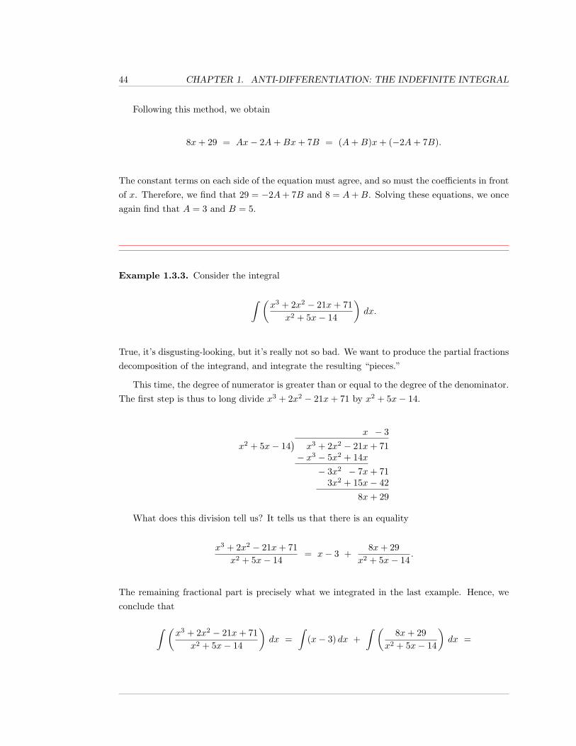
Example 1.3.3. Consider the integral
∫ (x3 + 2x2 − 21x+ 71
x2 + 5x− 14
)dx.
True, it’s disgusting-looking, but it’s really not so bad. We want to produce the partial fractionsdecomposition of the integrand, and integrate the resulting “pieces.”
This time, the degree of numerator is greater than or equal to the degree of the denominator.The first step is thus to long divide x3 + 2x2 − 21x+ 71 by x2 + 5x− 14.
x − 3x2 + 5x− 14
)x3 + 2x2 − 21x+ 71
− x3 − 5x2 + 14x− 3x2 − 7x+ 71
3x2 + 15x− 428x+ 29
What does this division tell us? It tells us that there is an equality
x3 + 2x2 − 21x+ 71x2 + 5x− 14
= x− 3 +8x+ 29
x2 + 5x− 14.
The remaining fractional part is precisely what we integrated in the last example. Hence, weconclude that
∫ (x3 + 2x2 − 21x+ 71
x2 + 5x− 14
)dx =
∫(x− 3) dx +
∫ (8x+ 29
x2 + 5x− 14
)dx =
1.3. INTEGRATION BY PARTIAL FRACTIONS 45
x2
2− 3x + 3 ln |x+ 7| + 5 ln |x− 2| + C.
Example 1.3.4. Consider the integral
∫x+ 1
(x− 5)(x2 + 6x+ 11)dx.
The numerator has smaller degree than the denominator, so there’s no need to long divide. Weeither need to factor x2 + 6x + 11, or complete the square. A few seconds of thought shouldconvince you that it doesn’t factor into linear terms with integer coefficients; still, it could factorwith real, but irrational coefficients, or be irreducible over the real numbers. Completing thesquare will tell us, either way. We add and subtract (6/2)2 = 9, and find
x2 + 6x+ 11 = x2 + 6x+ 9− 9 + 11 = (x+ 3)2 + 2.
This polynomial has no real roots, and so is irreducible (over the real numbers). What do wedo?
Now that we know that x2 +6x+11 is irreducible, we temporarily put off using that it equals(x+ 3)2 + 2. What we want to do now is write an equality of functions
x+ 1(x− 5)(x2 + 6x+ 11)
=?
x− 5+
?x2 + 6x+ 11
,
but what should the question marks be this time?
As before, it can be shown that there are unique polynomials that take the places of thesequestion marks and, because the rational function on the left has a numerator of smaller degreethan the denominator, the question marks are polynomials of smaller degree than the respectivedenominators. Thus, there exist unique constants A, B, and C such that
x+ 1(x− 5)(x2 + 6x+ 11)
=A
x− 5+
Bx+ C
x2 + 6x+ 11. (1.7)
We wish to determine A, B, and C.
Again, we clear the denominators by multiplying both sides of the equation by the bigdenominator on the left, and canceling. We obtain
46 CHAPTER 1. ANTI-DIFFERENTIATION: THE INDEFINITE INTEGRAL
x+ 1 = A(x2 + 6x+ 11) + (Bx+ C)(x− 5),
which now must hold for all x. Plugging in x = 5 immediately tells us that 6 = A · 66 +B · 0, sothat A = 1/11, but there are no easy (real) values to plug in for x to immediately yield B andC. We will multiply things out and match coefficients.
We find
x+ 1 = Ax2 + 6Ax+ 11A+Bx2 − 5Bx+ Cx− 5C =
(A+B)x2 + (6A− 5B + C)x+ (11A− 5C).
Therefore, noting that 0 is the coefficient of x2 in the polynomial x + 1, we obtain the threesimultaneous equations
A+B = 0, 6A− 5B + C = 1, and 11A− 5C = 1.
As we already know that A = 1/11, we really only need two of these equations, say the firstand the last, to find that B = −1/11 and C = 0. Substituting these values into Formula 1.7,we obtain
x+ 1(x− 5)(x2 + 6x+ 11)
=111·(
1x− 5
− x
x2 + 6x+ 11
).
Before integrating, we wish to rewrite x/(x2 + 6x + 11) in a different form. Recall that wecompleted the square to find that x2 + 6x+ 11 = (x+ 3)2 + 2. Thus,
x
x2 + 6x+ 11=
x
(x+ 3)2 + 2=
(x+ 3)− 3(x+ 3)2 + 2
,
where we added and subtracted a 3 in the numerator in order to have the same quantities inparentheses in the numerator and denominator. We shall see momentarily why this is useful.
Putting together all of our work above, we have
x+ 1(x− 5)(x2 + 6x+ 11)
=111
[1
x− 5− x+ 3
(x+ 3)2 + 2+ 3 · 1
(x+ 3)2 + 2
].
This, finally, is the partial fractions decomposition that we need. We now discuss how tointegrate the main “pieces” of the righthand side above, and will then put these pieces togetherto obtain the final answer.
1.3. INTEGRATION BY PARTIAL FRACTIONS 47
Certainly, the integral of 1/(x − 5) is easy. By making the substitution u = x − 5, we findquickly that ∫
1x− 5
dx = ln |x− 5|+ C1.
By making the substitution w = (x + 3)2 + 2, we find that dw = 2(x + 3) dx, and sodw/2 = (x+ 3) dx. Hence,
∫x+ 3
(x+ 3)2 + 2dx =
∫12· dww
=12
ln |w|+ C2 =12
ln((x+ 3)2 + 2
)+ C2,
where the absolute value signs disappeared since (x+ 3)2 + 2 ≥ 0.
If we let v = x+ 3, then dv = dx, and we find
∫1
(x+ 3)2 + 2dx =
∫1
v2 + (√
2)2dv,
which, by the second formula in Theorem 1.1.18, is equal to
1√2· tan−1
(v√2
)+ C3 =
1√2· tan−1
(x+ 3√
2
)+ C3.
Combining all of our work above, we, at long last, conclude that
∫x+ 1
(x− 5)(x2 + 6x+ 11)dx =
111
[ln |x− 5| − 1
2ln((x+ 3)2 + 2
)+
3√2· tan−1
(x+ 3√
2
)]+ C.
Example 1.3.5. As our final example of integration by partial fraction, we will calculate theintegral ∫
1(x+ 2)(x− 1)3(x2 + 4)
dx.
Note that the denominator of the integrand has a repeated linear factor, (x−1)3. This factoris, of course, a polynomial of degree 3, but it is important that it is a repeated linear term. As
48 CHAPTER 1. ANTI-DIFFERENTIATION: THE INDEFINITE INTEGRAL
you would expect, we want to find the partial fractions decomposition:
1(x+ 2)(x− 1)3(x2 + 4)
=A
x+ 2+
?(x− 1)3
+Bx+ C
x2 + 4,
where x2 + 4 is clearly an irreducible quadratic polynomial, and the question mark should bea general polynomial of degree 2, one degree less than the denominator. The slightly trickypoint is that, instead of writing the polynomial in the numerator of the (x− 1)3 term in powersof x, it is best to write it in powers on (x − 1). Thus, we replace the question mark withD(x− 1)2 + E(x− 1) + F . This yields a summand
D(x− 1)2 + E(x− 1) + F
(x− 1)3=
D
x− 1+
E
(x− 1)2+
F
(x− 1)3.
This leads to the general rule that, when looking for the partial fractions decompositionof a rational function, when there are repeated linear factors in the denominator, you havesummands of the form a constant over each repeated power of the repeated linear factor, up tothe power that appears in the original denominator. In a similar fashion, if we have repeatedpowers of an irreducible quadratic factor in the denominator, we have summands of the form ageneral linear polynomial over each repeated power of the repeated irreducible quadratic factor,up to the power that appears in the original denominator.
Hence, we want to find constants A through F such that
1(x+ 2)(x− 1)3(x2 + 4)
=
A
x+ 2+
D
x− 1+
E
(x− 1)2+
F
(x− 1)3+Bx+ C
x2 + 4. (1.8)
However, even before finding the constants, we can easily write the integral of this rationalfunction, with the unknown constants still to be determined. You should be able to show quicklythat ∫ (
A
x+ 2+
D
x− 1+
E
(x− 1)2+
F
(x− 1)3+
Bx
x2 + 4+
C
x2 + 4
)dx =
A ln |x+ 2| + D ln |x− 1| − E
x− 1− F
2(x− 1)2+
B
2ln(x2 + 4) +
C
2tan−1
(x2
)+K, (1.9)
where K is an arbitrary constant (which cannot be determined, unlike A through F ).
We need to find the constants A through F to finish the problem. You clear all the de-nominators in Formula 1.8 by multiplying both sides by the big denominator on the left, and
1.3. INTEGRATION BY PARTIAL FRACTIONS 49
obtain
1 = A(x− 1)3(x2 + 4) + D(x+ 2)(x− 1)2(x2 + 4) +
E(x+ 2)(x− 1)(x2 + 4) + F (x+ 2)(x2 + 4) + (Bx+ C)(x+ 2)(x− 1)3.
What a mess! Still A and F are easy to find; plug in x = −2 and x = 1. We find 1 =A(−2 − 1)3((−2)2 + 4) so that A = −1/216, and 1 = F (1 + 2)(12 + 4), so that F = 1/15. Tofind the remaining constants in the partial fractions decomposition, we leave it as an exercise (ahorrible exercise) for you to expand the terms, collect the powers of x, match the coefficients, andsolve the resulting simultaneous equations. Alternatively, many calculators, computer programs,and the web site wolframalpha.com can produce partial fractions decompositions. What youshould find is that B = −9/1000, C = 13/500, D = 46/3375, and E = −11/225. Now, yousubstitute the values of A through F into Formula 1.9, and you’re finished.
As we saw in the examples above, there are always two major steps in using partial fractionsto integrate a rational function f(x):
• Find the partial fractions decomposition of f(x).
• Integrate each summand in the partial fractions decomposition.
Of course, we have yet to state exactly what the partial fractions decomposition for anarbitrary rational function is. We shall do so now.
Suppose n(x) and q(x) are (real) polynomial functions, and that the leading coefficient ofq(x) is a 1, i.e., q(x) is not the zero function, and the coefficient of the largest power of xappearing in q(x), with a non-zero coefficient, is a 1. (If the leading coefficient of q(x) were someother (non-zero) constant c, immediately factor out the c, follow the procedure given below, andthen, in the end, multiply by 1/c.)
We want to define the partial fractions decomposition of the rational function f(x) =n(x)/q(x), whose domain is all x such that q(x) 6= 0.
1. If the degree of n(x) is greater than, or equal to, the degree of q(x), then you first (long)divide q(x) into n(x); if what you obtain from the division is a polynomial p(x) and aremainder of r(x), then exactly what that means is that
f(x) =n(x)q(x)
= p(x) +r(x)q(x)
,
50 CHAPTER 1. ANTI-DIFFERENTIATION: THE INDEFINITE INTEGRAL
where r(x) = 0 or has degree less than the degree of q(x). As it is easy to integratethe polynomial portion p(x), we will concentrate on the portion r(x)/q(x). In addition, ifr(x) = 0, then there is nothing left to do, so we will assume that r(x) 6= 0.
So, at this point, we want to define and integrate the partial fractions decomposition ofr(x)/q(x), where r(x) and q(x) are polynomials, r(x) 6= 0, q(x) 6= 0, the degree of r(x) isstrictly less than the degree of q(x), and the leading coefficient of q(x) equals 1.
2. Factor q(x) into, possibly repeated, linear terms, each of the form (x− r)m, and, possiblyrepeated, irreducible quadratic terms, which, after completing the square, can each bewritten in the form [(x− r)2 + b2]m.
3. r(x)/q(x) is equal to a sum of contributions, where you have a contribution from each,possibly repeated, irreducible factor of q(x). For a factor of the form (x − r)m, thecontribution to the partial fractions decomposition is a sum of the form
A1
x− r+
A2
(x− r)2+ · · ·+ Am
(x− r)m,
where all of the Ai’s are constants (to be determined).
For a factor of the form [(x− r)2 + b2]m, the contribution to the partial fractions decom-position is a sum of the form
B1(x− r) + C1
(x− r)2 + b2+B2(x− r) + C2
[(x− r)2 + b2]2+ · · ·+ Bm(x− r) + Cm
[(x− r)2 + b2]m,
where all of the Bi’s and Ci’s are constants (to be determined).
4. Now, set r(x)/q(x) equal to the sum of all of the contributions described above, and clearthe denominators by multiplying both sides of the equation by q(x), and canceling factors.The result is that the polynomial r(x) equals a sum of polynomials with (possibly many)unknown constants; these polynomial functions must be equal for all x.
5. Determine the unknown constants above by plugging in exceptional values (roots of q(x))for x, or by multiplying out the entire righthand side, gathering the powers of x together,and matching coefficients with the coefficients of r(x). A combination of these two methodsmay be easiest.
6. After determining all of the constants, the sum of the contributions described above, withthe all of the values of the Ai’s, Bi’s, and Ci’s inserted is the partial fractions decompositionof r(x)/q(x).
7. The individual summands in the partial fractions decomposition are integrated as follows.We will omit the arbitrary constants produced by the indefinite integral.
The integrals with powers of a linear factor are easy:
1.3. INTEGRATION BY PARTIAL FRACTIONS 51
∫A
x− rdx = A ln |x− r|,
and if m ≥ 2, ∫A
(x− r)mdx =
A(x− r)−m+1
−m+ 1
The integrals with powers of an irreducible quadratic term are harder:
∫B(x− r) + C
[(x− r)2 + b2]mdx =
∫B(x− r)
[(x− r)2 + b2]mdx +
∫C
[(x− r)2 + b2]mdx.
In the first integral, the substitution u = (x− r)2 + b2 yields du = 2(x− r) dx, so that wehave ∫
B(x− r)[(x− r)2 + b2]m
dx =B
2
∫du
um,
which, if m = 1, isB
2ln |u| = B
2ln((x− r)2 + b2)
and, if m ≥ 2, isB
2· u−m+1
−m+ 1=
B
2· ((x− r)2 + b2)−m+1
−m+ 1.
Finally, we need to integrate terms of the form
∫C
[(x− r)2 + b2]mdx.
After pulling the constant C outside the integral, and making the trivial substitutionu = x − r, we are reduced to an integral of the form in Example 1.2.8; see that examplefor the technique.
1.3.1 Exercises
Use partial fractions to calculate the anti-derivatives in Exercises 1-25.
1.∫
11x+ 26x2 + 5x+ 6
dx
2.∫
t+ 58t2 + 6t− 16
dt
52 CHAPTER 1. ANTI-DIFFERENTIATION: THE INDEFINITE INTEGRAL
3.∫
8u− 35u2 − 7u
du
4.∫−42
y2 − 49dy
5.∫
11z − 22z2 − z − 1
dz
6.∫
2w3 + 6w2 − 4w + 11w2 + 3w − 4
dw
7.∫p2 + p+ 3p+ 3
dp
8.∫−2θ3 + 4θ2 + 6θ − 2
θ2 − 1dθ
9.∫x3 + 12x2 + 51x+ 74
x2 + 8x+ 15dx
10.∫s3 + 7s2 + s+ 10
s+ 7ds
11.∫
7m2 + 12m+ 8(m+ 3)(m2 +m+ 1)
dm
12.∫
6n2 − 4n+ 20(n− 2)(n2 + 5)
dn
13.∫
−3v2 + 4v − 66(v − 6)(v2 − 4v + 18)
dv
14.∫
3rr4 + 5r2 + 4
dr
15.∫
12t2 + 52t+ 150(t2 + 5t+ 30)(2t+ 3)
dt
16.∫
3x2 + 8x+ 5(x2 + 2x+ 5)(x+ 3)
dx
17.∫
−2y2 − 60(y2 + 4y + 20)(y + 12)
dy
18.∫
1− 2w(w − 1)(w2 + w + 1)
dw
19.∫
−3φ2 − 30(φ2 + φ+ 5)(φ+ 2)
dφ
20.∫
4s2 + 4s+ 6(s2 − s+ 3)(s+ 3)
ds
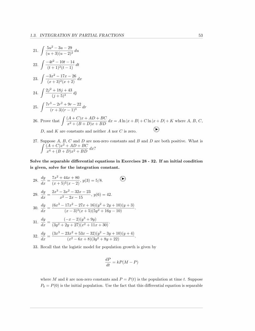
1.3. INTEGRATION BY PARTIAL FRACTIONS 53
21.∫
5u2 − 3u− 29(u+ 3)(u− 2)2
du
22.∫−4t2 − 10t− 14(t+ 1)2(t− 1)
dt
23.∫−3x2 − 17x− 26(x+ 3)2(x+ 2)
dx
24.∫
2j2 + 18j + 43(j + 5)3
dj
25.∫
7r3 − 2r2 + 9r − 22(r + 3)(r − 1)3
dr
26. Prove that∫
(A+ C)x+AD +BC
x2 + (B +D)x+BDdx = A ln |x+B|+C ln |x+D|+K where A, B, C,
D, and K are constants and neither A nor C is zero.
27. Suppose A, B, C and D are non-zero constants and B and D are both positive. What is∫(A+ C)x2 +AD +BC
x4 + (B +D)x2 +BDdx?
Solve the separable differential equations in Exercises 28 - 32. If an initial condition
is given, solve for the integration constant.
28.dy
dx=
7x2 + 44x+ 80(x+ 5)2(x− 2)
, y(3) = 5/8.
29.dy
dx=
2x3 − 3x2 − 32x− 23x2 − 2x− 15
, y(6) = 42.
30.dy
dx=
(6x3 − 17x2 − 27x+ 16)(y2 + 2y + 10)(y + 3)(x− 3)3(x+ 5)(5y2 + 16y − 10)
.
31.dy
dx=
(−x− 2)(y3 + 9y)(3y2 + 2y + 27)(x2 + 11x+ 30)
.
32.dy
dx=
(3x3 − 23x2 + 53x− 32)(y2 − 3y + 10)(y + 4)(x2 − 6x+ 8)(3y2 + 8y + 22)
.
33. Recall that the logistic model for population growth is given by
dP
dt= kP (M − P )
where M and k are non-zero constants and P = P (t) is the population at time t. SupposeP0 = P (0) is the initial population. Use the fact that this differential equation is separable
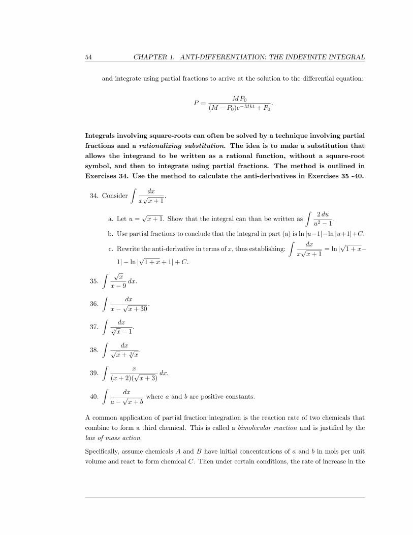
54 CHAPTER 1. ANTI-DIFFERENTIATION: THE INDEFINITE INTEGRAL
and integrate using partial fractions to arrive at the solution to the differential equation:
P =MP0
(M − P0)e−Mkt + P0.
Integrals involving square-roots can often be solved by a technique involving partial
fractions and a rationalizing substitution. The idea is to make a substitution that
allows the integrand to be written as a rational function, without a square-root
symbol, and then to integrate using partial fractions. The method is outlined in
Exercises 34. Use the method to calculate the anti-derivatives in Exercises 35 -40.
34. Consider∫
dx
x√x+ 1
.
a. Let u =√x+ 1. Show that the integral can than be written as
∫2 duu2 − 1
.
b. Use partial fractions to conclude that the integral in part (a) is ln |u−1|−ln |u+1|+C.
c. Rewrite the anti-derivative in terms of x, thus establishing:∫
dx
x√x+ 1
= ln |√
1 + x−
1| − ln |√
1 + x+ 1|+ C.
35.∫ √
x
x− 9dx.
36.∫
dx
x−√x+ 30
.
37.∫
dx3√x− 1
.
38.∫
dx√x+ 3√x
.
39.∫
x
(x+ 2)(√x+ 3)
dx.
40.∫
dx
a−√x+ b
where a and b are positive constants.
A common application of partial fraction integration is the reaction rate of two chemicals thatcombine to form a third chemical. This is called a bimolecular reaction and is justified by thelaw of mass action.
Specifically, assume chemicals A and B have initial concentrations of a and b in mols per unitvolume and react to form chemical C. Then under certain conditions, the rate of increase in the
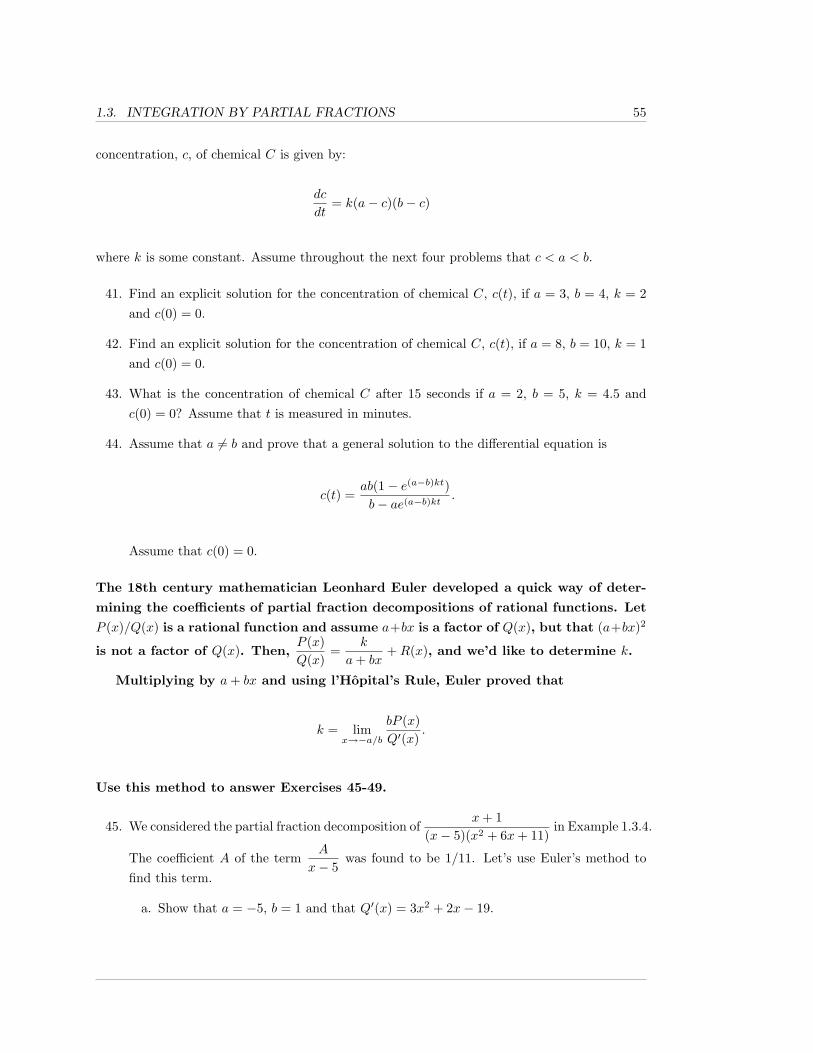
1.3. INTEGRATION BY PARTIAL FRACTIONS 55
concentration, c, of chemical C is given by:
dc
dt= k(a− c)(b− c)
where k is some constant. Assume throughout the next four problems that c < a < b.
41. Find an explicit solution for the concentration of chemical C, c(t), if a = 3, b = 4, k = 2and c(0) = 0.
42. Find an explicit solution for the concentration of chemical C, c(t), if a = 8, b = 10, k = 1and c(0) = 0.
43. What is the concentration of chemical C after 15 seconds if a = 2, b = 5, k = 4.5 andc(0) = 0? Assume that t is measured in minutes.
44. Assume that a 6= b and prove that a general solution to the differential equation is
c(t) =ab(1− e(a−b)kt)b− ae(a−b)kt .
Assume that c(0) = 0.
The 18th century mathematician Leonhard Euler developed a quick way of deter-
mining the coefficients of partial fraction decompositions of rational functions. Let
P (x)/Q(x) is a rational function and assume a+bx is a factor of Q(x), but that (a+bx)2
is not a factor of Q(x). Then,P (x)Q(x)
=k
a+ bx+R(x), and we’d like to determine k.
Multiplying by a+ bx and using l’Hopital’s Rule, Euler proved that
k = limx→−a/b
bP (x)Q′(x)
.
Use this method to answer Exercises 45-49.
45. We considered the partial fraction decomposition ofx+ 1
(x− 5)(x2 + 6x+ 11)in Example 1.3.4.
The coefficient A of the termA
x− 5was found to be 1/11. Let’s use Euler’s method to
find this term.
a. Show that a = −5, b = 1 and that Q′(x) = 3x2 + 2x− 19.
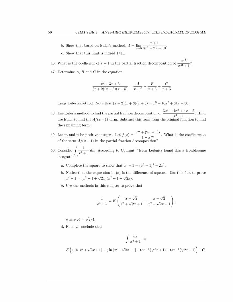
56 CHAPTER 1. ANTI-DIFFERENTIATION: THE INDEFINITE INTEGRAL
b. Show that based on Euler’s method, A = limx→5
x+ 13x2 + 2x− 10
.
c. Show that this limit is indeed 1/11.
46. What is the coefficient of x+ 1 in the partial fraction decomposition ofx13
x23 + 1?
47. Determine A, B and C in the equation
x2 + 3x+ 5(x+ 2)(x+ 3)(x+ 5)
=A
x+ 2+
B
x+ 3+
C
x+ 5
using Euler’s method. Note that (x+ 2)(x+ 3)(x+ 5) = x3 + 10x2 + 31x+ 30.
48. Use Euler’s method to find the partial fraction decomposition of3x3 + 4x2 + 4x+ 5
x4 − 1. Hint:
use Euler to find the A/(x−1) term. Subtract this term from the original function to findthe remaining term.
49. Let m and n be positive integers. Let f(x) =xm + (2n− 1)x
1− x2n. What is the coefficient A
of the term A/(x− 1) in the partial fraction decomposition?
50. Consider∫
1x4 + 1
dx. According to Courant, ”Even Leibnitz found this a troublesome
integration.”
a. Complete the square to show that x4 + 1 = (x2 + 1)2 − 2x2.
b. Notice that the expression in (a) is the difference of squares. Use this fact to provex4 + 1 = (x2 + 1 +
√2x)(x2 + 1−
√2x).
c. Use the methods in this chapter to prove that
1x4 + 1
= K
(x+√
2x2 +
√2x+ 1
− x−√
2x2 −
√2x+ 1
),
where K =√
2/4.
d. Finally, conclude that ∫dx
x4 + 1=
K(
12 ln |x2 +
√2x+ 1|− 1
2 ln |x2−√
2x+ 1|+ tan−1(√
2x+ 1) + tan−1(√
2x−1))
+C.
1.4. INTEGRATION USING HYPERBOLIC SINE AND COSINE 57
1.4 Integration usingHyperbolic Sine and Cosine
Corresponding to sine and cosine, we will define the hyperbolic sine and hyperbolic cosine func-tions, f(x) = sinhx and g(x) = coshx, respectively; when speaking, hyperbolic cosine is usuallyreferred to by pronouncing cosh phonetically, while hyperbolic sine is usually referred to bypronouncing sinh as though it were the word cinch.
Once we have hyperbolic sine and cosine, we could, but will not, define the remaining fourhyperbolic trig. functions, in analogy with how the other trig. functions are defined in terms ofsine and cosine, e.g., hyperbolic tangent is hyperbolic sine divided by hyperbolic cosine.
Instead, we will concentrate on the properties of sinh and cosh which make them so usefulfor anti-differentiating certain types of functions.
The definitions of hyperbolic sine and cosine do not look analogous in any way to the defini-tions of the usual sine and cosine functions. Later, in Example 4.6.21, we will see that Euler’sFormula provides a close relationship between the hyperbolic and standard trig. functions, butyou have to be willing to deal with complex numbers.
Definition 1.4.1. The hyperbolic sine function, sinh : R→ R, is defined by
sinhx =ex − e−x
2,
and the hyperbolic cosine function, cosh : R→ R, is defined by
coshx =ex + e−x
2.
The following algebraic/graphical/Calculus properties of sinh and cosh are easy to verify,and we leave them as exercises.
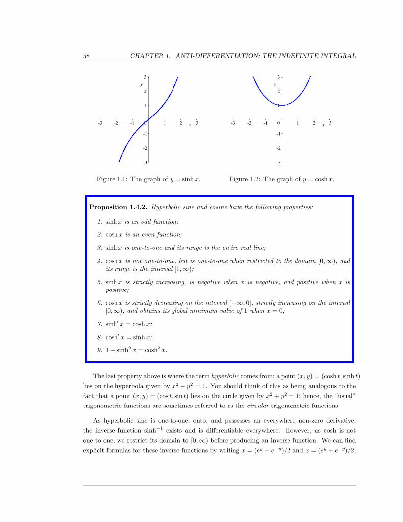
58 CHAPTER 1. ANTI-DIFFERENTIATION: THE INDEFINITE INTEGRAL
-3 -2 -1 0 1 2 3
-3
-2
-1
1
2
3
Figure 1.1: The graph of y = sinhx.
-3 -2 -1 0 1 2 3
-3
-2
-1
1
2
3
Figure 1.2: The graph of y = coshx.
Proposition 1.4.2. Hyperbolic sine and cosine have the following properties:
1. sinhx is an odd function;
2. coshx is an even function;
3. sinhx is one-to-one and its range is the entire real line;
4. coshx is not one-to-one, but is one-to-one when restricted to the domain [0,∞), andits range is the interval [1,∞);
5. sinhx is strictly increasing, is negative when x is negative, and positive when x ispositive;
6. coshx is strictly decreasing on the interval (−∞, 0], strictly increasing on the interval[0,∞), and obtains its global minimum value of 1 when x = 0;
7. sinh′ x = coshx;
8. cosh′ x = sinhx;
9. 1 + sinh2 x = cosh2 x.
The last property above is where the term hyperbolic comes from; a point (x, y) = (cosh t, sinh t)lies on the hyperbola given by x2 − y2 = 1. You should think of this as being analogous to thefact that a point (x, y) = (cos t, sin t) lies on the circle given by x2 + y2 = 1; hence, the “usual”trigonometric functions are sometimes referred to as the circular trigonometric functions.
As hyperbolic sine is one-to-one, onto, and possesses an everywhere non-zero derivative,the inverse function sinh−1 exists and is differentiable everywhere. However, as cosh is notone-to-one, we restrict its domain to [0,∞) before producing an inverse function. We can findexplicit formulas for these inverse functions by writing x = (ey − e−y)/2 and x = (ey + e−y)/2,
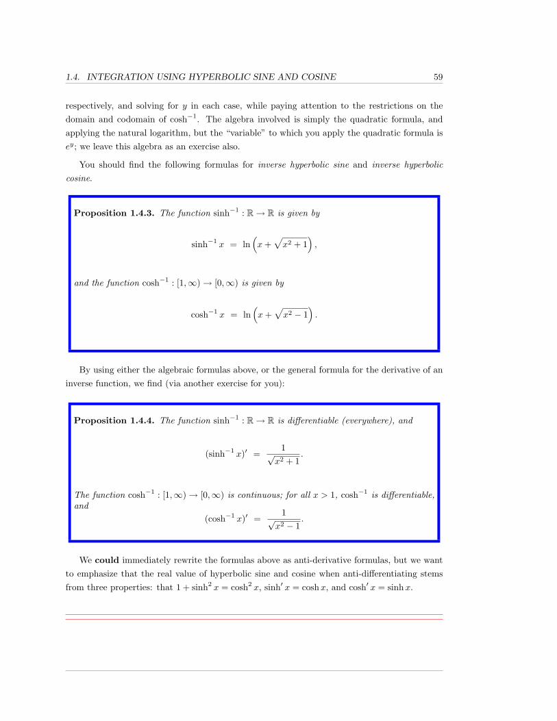
1.4. INTEGRATION USING HYPERBOLIC SINE AND COSINE 59
respectively, and solving for y in each case, while paying attention to the restrictions on thedomain and codomain of cosh−1. The algebra involved is simply the quadratic formula, andapplying the natural logarithm, but the “variable” to which you apply the quadratic formula isey; we leave this algebra as an exercise also.
You should find the following formulas for inverse hyperbolic sine and inverse hyperboliccosine.
Proposition 1.4.3. The function sinh−1 : R→ R is given by
sinh−1 x = ln(x+
√x2 + 1
),
and the function cosh−1 : [1,∞)→ [0,∞) is given by
cosh−1 x = ln(x+
√x2 − 1
).
By using either the algebraic formulas above, or the general formula for the derivative of aninverse function, we find (via another exercise for you):
Proposition 1.4.4. The function sinh−1 : R→ R is differentiable (everywhere), and
(sinh−1 x)′ =1√
x2 + 1.
The function cosh−1 : [1,∞)→ [0,∞) is continuous; for all x > 1, cosh−1 is differentiable,and
(cosh−1 x)′ =1√
x2 − 1.
We could immediately rewrite the formulas above as anti-derivative formulas, but we wantto emphasize that the real value of hyperbolic sine and cosine when anti-differentiating stemsfrom three properties: that 1 + sinh2 x = cosh2 x, sinh′ x = coshx, and cosh′ x = sinhx.
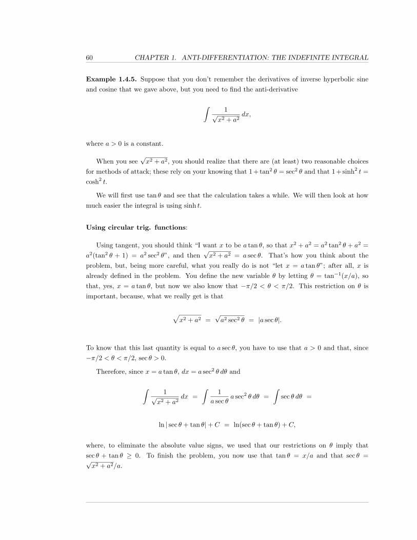
60 CHAPTER 1. ANTI-DIFFERENTIATION: THE INDEFINITE INTEGRAL
Example 1.4.5. Suppose that you don’t remember the derivatives of inverse hyperbolic sineand cosine that we gave above, but you need to find the anti-derivative
∫1√
x2 + a2dx,
where a > 0 is a constant.
When you see√x2 + a2, you should realize that there are (at least) two reasonable choices
for methods of attack; these rely on your knowing that 1 + tan2 θ = sec2 θ and that 1 + sinh2 t =cosh2 t.
We will first use tan θ and see that the calculation takes a while. We will then look at howmuch easier the integral is using sinh t.
Using circular trig. functions:
Using tangent, you should think “I want x to be a tan θ, so that x2 + a2 = a2 tan2 θ + a2 =a2(tan2 θ + 1) = a2 sec2 θ”, and then
√x2 + a2 = a sec θ. That’s how you think about the
problem, but, being more careful, what you really do is not “let x = a tan θ”; after all, x isalready defined in the problem. You define the new variable θ by letting θ = tan−1(x/a), sothat, yes, x = a tan θ, but now we also know that −π/2 < θ < π/2. This restriction on θ isimportant, because, what we really get is that
√x2 + a2 =
√a2 sec2 θ = |a sec θ|.
To know that this last quantity is equal to a sec θ, you have to use that a > 0 and that, since−π/2 < θ < π/2, sec θ > 0.
Therefore, since x = a tan θ, dx = a sec2 θ dθ and
∫1√
x2 + a2dx =
∫1
a sec θa sec2 θ dθ =
∫sec θ dθ =
ln | sec θ + tan θ|+ C = ln(sec θ + tan θ) + C,
where, to eliminate the absolute value signs, we used that our restrictions on θ imply thatsec θ + tan θ ≥ 0. To finish the problem, you now use that tan θ = x/a and that sec θ =√x2 + a2/a.
1.4. INTEGRATION USING HYPERBOLIC SINE AND COSINE 61
Our final result:
∫1√
x2 + a2dx = ln
(x
a+√x2 + a2
a
)+ C = ln
(x+
√x2 + a2
)+ C,
where, in the last step, we used that ln[(x+√x2 + a2
)/a]
= ln(x+√x2 + a2
)− ln a, and then
we “absorbed” the − ln a into the constant C.
Using hyperbolic trig. functions:
Using hyperbolic sine, you should think “I want x to be a sinh t, so that x2 +a2 = a2 sinh2 t+a2 = a2(sinh2 t + 1) = a2 cosh2 t”, and then
√x2 + a2 = a cosh t. Again, that’s how you think
about the problem, but what you really do is not “let x = a sinh t”; you define the new variablet by letting t = sinh−1(x/a). However, we don’t need any special restrictions on t to know that√a2 cosh2 t = a cosh t, because cosh t ≥ 1 ≥ 0.
As x = a sinh t, dx = a cosh t dt, and we find
∫1√
x2 + a2dx =
∫1
a cosh ta cosh t dt =
∫1 dt = t+ C = sinh−1
(xa
)+ C,
which is the nicest form in which to leave the answer. On the other hand, if you wish to seethat this answer agrees with the answer that we obtained above, using tangent, then you usethe formula for sinh−1 in Proposition 1.4.3.
Example 1.4.6. Suppose that a > 0, and that we want the general anti-derivative of the
function f(x) =1√
x2 − a2with domain x > a, i.e., we want to find
∫1√
x2 − a2dx,
where x > a > 0.
We want x = a cosh t, so that
√x2 − a2 =
√a2 cosh2 t− a2 = a
√sinh2 t = a| sinh t|.
62 CHAPTER 1. ANTI-DIFFERENTIATION: THE INDEFINITE INTEGRAL
Thus, we let t = cosh−1(x/a), which implies both that x = a cosh t and, as x/a > 1, that t > 0.Since t > 0, | sinh t| = sinh t.
Therefore, dx = a sinh t dt and
∫1√
x2 − a2dx =
∫1
a sinh ta sinh t dt =
∫1 dt = t+ C = cosh−1
(xa
)+ C.
The results from the last two examples are worth recording in a proposition.
Proposition 1.4.7. Suppose that a > 0. Then,
∫1√
x2 + a2dx = sinh−1
(xa
)+ C,
and, for x > a, ∫1√
x2 − a2dx = cosh−1
(xa
)+ C.
1.4.1 Exercises
Calculate the anti-derivatives of the functions.
1.∫
7√x2 + 9
dx.
2.∫
12√z2 − 625
dz.
3.∫
dy√4y2 + 49
.
4.∫
dt√7t2 − 81
.
5.∫
cosh(3x) dx.
1.4. INTEGRATION USING HYPERBOLIC SINE AND COSINE 63
6.∫s sinh s ds.
7.∫
2x√x4 + 9
dx.
8.∫
cosh2 z − sinh2 z dz. Hint: why is this trivial?
9.∫
dx√4x2 + 4x+ 9
.
10.∫
dy√y2 − 10y + 9
.
11.∫
1 +√t3 + 3t√
t2 + 3dt, t > 0.
12.∫ √
u2 − 4 +√u2 − 4√
u4 − 16du.
13.∫ √
x2 − 4 +√x2 + 9√
x4 + 5x2 − 36dx.
14.∫
u2
(u2 + 10)3/2du.
15.
a. Calculate∫
sinhx coshx dx using integration by parts.
b. Calculate∫
sinhx coshx dx directly by writing sinhx and coshx in terms of their
definitions using the exponential function.
16. Calculate∫ √
x2 + 1 dx.
In each of Exercises 17 through 25, prove the given statements from Proposi-
tion 1.4.2.
17. sinhx is an odd function.
18. coshx is an even function.
19. sinhx is one-to-one and its range is the entire real line.
20. coshx is not one-to-one, but is one-to-one when restricted to the domain [0,∞), and itsrange is the interval [1,∞).
64 CHAPTER 1. ANTI-DIFFERENTIATION: THE INDEFINITE INTEGRAL
21. sinhx is strictly increasing, is negative when x is negative, and positive when x is positive.
22. coshx is strictly decreasing on the interval (−∞, 0], strictly increasing on the interval[0,∞), and obtains its global minimum value of 1 when x = 0.
23. sinh′ x = coshx.
24. cosh′ x = sinhx.
25. 1 + sinh2 x = cosh2 x.
26. What is∫ √
x2 − 1 dx?
27. What is∫x2√x2 − 1 dx?
28. What is∫x2√x2 + 1 dx?
29. More generally, what is∫x2√x2 + a2 dx?
Use the previous four problems to calculate the integrals in the next four problems.
30.∫ √
9x2 − 16 dx.
31.∫
25x2√
25x2 − 1 dx.
32.∫ √
x6 + 100x4 dx.
33.∫cx2√b2x2 + a2 dx, b > 0, a > 0.
In exercises 34 though 37, you are given the acceleration function of a particle and
the velocity at one specific time. Find the velocity function.
34. a(t) =1√
t2 + 16t+ 25, v(0) = 10. Assume that t > −8 +
√39.
35. a(t) =1√
t2 − 6t+ 16, v(6) = 8.
36. a(t) =12√
6t2 + 24, v(3) = 6.
37. a(t) = 2t cosh(t2 + 2), v(0) = 4.
1.4. INTEGRATION USING HYPERBOLIC SINE AND COSINE 65
38. What is∫
sinh−1 x dx? Hint: use a technique similar to the one used in calculating∫lnx dx.
39. What is∫
cosh−1 x dx?
In the next four exercises you are given the acceleration function of a particle. Find
a formula for the position vector. Make sure to retain any integration constants.
Use the previous two problems.
40. a(t) =1√t2 + 9
.
41. a(t) =1√
t2 − 16.
42. a(t) =5√
4t2 + 25, v(0) = 0.
43. a(t) =6√
9t2 − 11, v(2) = 8.
Solve the following separable differential equations.
44.dx
dt=√
12x2 − 84 + 6t2
.
45.dx
dt=
(x2 + 1)3/2
(√t2 − 3)
.
46.dx
dt=et(x+1) − et(x−1)
ex(t+1) + ex(t−1).
47.dx
dt=
√x4 + x2 + t2 + t2x2
t4 − t2 − x2 + t2x2. Hint: look for a factor common to the numerator and
denominator.
Calculate the integrals of the following products of hyperbolic and trigonometric
functions. You may find it easier write the hyperbolic functions in terms of expo-
nential functions.
48.∫
sinhx cosx dx.
49.∫
coshx cosx dx.
50.∫
coshx sinhx sinx cosx dx.

66 CHAPTER 1. ANTI-DIFFERENTIATION: THE INDEFINITE INTEGRAL
Chapter 2
Continuous sums: the DefiniteIntegral
As we wrote at the beginning of the previous chapter, the definite integral is the mathematicallyprecise notion of what it means to “take a continuous sum of infinitesimal contributions.” Itis the definition of integration as a continuous sum that yields all of its applications, many ofwhich we will look at in Chapter 3. However, the basic method of calculating definite integralsis to use the Fundamental Theorem of Calculus, Theorem 2.4.10, to conclude that the problemof calculation of an integral (typically) boils down to producing an anti-derivative. Thus, as wewrote in the previous chapter, anti-differentiation is also referred to as calculating an indefiniteintegral.
We begin this chapter with a discussion of basic properties, notations, and techniques involv-ing summations; not surprisingly, differences are involved in crucial ways. We then move on tothe problem of how to approximate a “continuous sum”; of course, part of the problem is thatwe don’t (yet) have a mathematically rigorous definition of what a continuous sum is. Afterwe have our approximations, we then use limits of our approximations to define the definiteintegral.
67
68 CHAPTER 2. CONTINUOUS SUMS: THE DEFINITE INTEGRAL
2.1 Sums and Differences
In this section, we need to recall some notation and properties related to summations. We shallalso define the difference operator, and use it to derive some useful summation formulas.
Recall the sigma notation for summations.
Definition 2.1.1. Suppose that we have two integers m and n, where m ≤ n, we let [m..n]denote the set of integers between, or equal to, m and n. We call such a set an integerinterval.
Suppose we have a function f , whose domain includes [m..n]. Then, we writen∑
k=m
f(k) for
the summation, as k goes from m to n, of f(k). This means that
n∑k=m
f(k) = f(m) + f(m+ 1) + · · ·+ f(n− 1) + f(n).
In this context k is frequently referred to as the index of summation, and f(k) is frequentlywritten as fk. The integer interval [m..n] is called the range of the index of summation.
For example,3∑
k=−1
k2 = (−1)2 + 02 + 12 + 22 + 32 = 15,
or, as another example,
p(x) = a0 + a1x+ · · ·+ anxn =
n∑k=0
akxk,
where x0 in the summation is to be interpreted as equaling 1, even if x = 0.
Note that the indexing variable k is a dummy variable; if we replaced it with an i or j, or
2.1. SUMS AND DIFFERENCES 69
any other variable (which is not already present), the summation would not change, e.g.,
3∑j=−1
j2 = (−1)2 + 02 + 12 + 22 + 32 = 15,
Summations can be “split”. For instance, in the example above,
3∑j=−1
j2 = (−1)2 + 02 + 12 + 22 + 32 =
[(−1)2 + 02
]+[12 + 22 + 32
]=
0∑j=−1
j2 +3∑j=1
j2.
In general, we have
Proposition 2.1.2. (splitting summations) If m, n, and p are integers, with m ≤ n ≤ p,and f is a function whose domain includes the integer interval [m..p], then
p∑k=m
fk =n∑
k=m
fk +p∑
k=n+1
fk,
where, if n = p, the last summation should be interpreted as being 0.
Looking once again at
3∑j=−1
j2 = (−1)2 + 02 + 12 + 22 + 32,
we note that we can replace each term j2 by((j + 6) − 6
)2 (which may seem like a silly thingto do, but it leads us to an important property); this means that we have the easy equality
(−1)2 + 02 + 12 + 22 + 32 = (6− 7)2 + (7− 7)2 + (8− 7)2 + (9− 7)2 + (10− 7)2,
70 CHAPTER 2. CONTINUOUS SUMS: THE DEFINITE INTEGRAL
which equals10∑k=6
(k − 7)2.
In general,
Proposition 2.1.3. (shifting indices) Suppose we have a function f , whose domain in-cludes the integer interval [m..n]. Let p be an integer.Then, by making the substitution k = j + p, so that j = k − p, we obtain
n∑j=m
fj =n+p∑
k=m+p
fk−p.
Thus, you get the same sum if you add p to each of the bounds of the summation, and simulta-neously replace each occurrence of the index k by k minus p.
Consider now9∑k=7
(1.7k2 −
√3 sin k
)=
(1.7(7)2 −
√3 sin(7)
)+(1.7(8)2 −
√3 sin(8)
)+(1.7(9)2 −
√3 sin(9)
)=
1.7(72 + 82 + 92
)+ (−
√3)(
sin 7 + sin 8 + sin 9)
=
1.79∑k=7
k2 + (−√
3)9∑k=7
sin k.
More generally, the algebraic properties of real numbers (i.e., associativity, commutativity,and distributivity) immediately imply:
Proposition 2.1.4. (linearity of summation) If a and b are constants, and f and g arefunctions whose domain includes the integer interval [m..n], then
n∑k=m
(afk + bgk
)= a
n∑k=m
fk + b
n∑k=m
gk.
2.1. SUMS AND DIFFERENCES 71
Example 2.1.5. The properties of summations described above may seem simple, but theyallow us to derive formulas involving sums that really don’t look so obvious. Consider, forinstance, the problem of “simplifying”
250∑k=3
k(k − 1) −50∑k=1
(k + 1)(k + 2). (2.1)
We would like to combine the two summations, using linearity; however, the ranges of theindices of summation would need to be the same, and they are not. We will fix this “problem”in two different ways. Understand that the point of this example is not that you will necessarilyagree that what we end up with is simpler than what we started with; the point is for you tounderstand the types of manipulations that we use.
First approach: We split the second summation, and have
250∑k=3
k(k − 1) −50∑k=1
(k + 1)(k + 2) =
250∑k=3
k(k − 1) −50∑k=3
(k + 1)(k + 2) −2∑k=1
(k + 1)(k + 2).
Now we can use linearity on the first two of the three summations above to obtain
50∑k=3
[2k(k − 1)− (k + 1)(k + 2)
]−
2∑k=1
(k + 1)(k + 2) =
[50∑k=3
(2k2 − 2k − k2 − 3k − 2
)]− 6 − 12 =
−18 +50∑k=3
(k2 − 5k − 2
)Second approach: We first shift the index in the second summation in Formula 2.1; we add 2to each of the bounds and replace k by (k − 2) in the summation. We obtain
250∑k=3
k(k − 1) −50∑k=1
(k + 1)(k + 2) =
72 CHAPTER 2. CONTINUOUS SUMS: THE DEFINITE INTEGRAL
250∑k=3
k(k − 1) −52∑k=3
((k − 2) + 1
)((k − 2) + 2
)=
250∑k=3
k(k − 1) −52∑k=3
(k − 1)k.
The range of the index of summation on the right above still does not match that of thesummation on the left, but we can split off part of the sum
250∑k=3
k(k − 1) −52∑k=3
(k − 1)k.
250∑k=3
k(k − 1) −
[50∑k=3
k(k − 1)
]− (50)(51) − (51)(52) =
− (50)(51) − (51)(52) +50∑k=3
[2k(k − 1)− k(k − 1)
]=
− (50)(51) − (51)(52) +50∑k=3
[k(k − 1)
],
which does not look very similar to our answer from the first approach, but is nonetheless equallycorrect.
We now want to define notation related to differences.
Definition 2.1.6. Suppose that m and n are integers, and m < n, and suppose that we havea real function f , whose domain is [m..n]. Then, we define the finite difference function∆f to be the function with domain [(m+ 1)..n] given by
(∆f)(k) = f(k)− f(k − 1).
2.1. SUMS AND DIFFERENCES 73
Remark 2.1.7. We have been very formal with our notation above. Typically, we write thingslike ∆k2 = k2 − (k − 1)2 = k2 − (k2 − 2k + 1) = 2k − 1, in place of writing that, if f(k) = k2,then (∆f)(k) = 2k − 1.
We should also remark that, in the notation [m..n], we mean to allow the cases wherem = −∞ and/or n =∞. To be precise, we mean that, if m and n are integers, then
[−∞..n] = {k | k is an integer, and k ≤ n},
[m..∞] = {k | k is an integer, and m ≤ k},
and [−∞..∞] is the entire set of integers.
Finally, in Definition 2.1.6, if m = −∞, then the m+ 1 which appears in the domain of ∆fshould also be taken to equal −∞.
Like summations, the finite difference operator is linear.
Proposition 2.1.8. (linearity of differences) If a and b are constants, and f and g arefunctions whose domain is [m..n], then
∆(af(k) + bg(k)
)= a∆f(k) + b∆g(k).
Despite the fact that it is trivial to prove, the following result turns out to be very useful.
Proposition 2.1.9. (telescoping sums) Suppose that m and n are integers, and m < n.If f is a real function, whose domain is [m..n], then
n∑k=m+1
∆f(k) = f(n)− f(m).
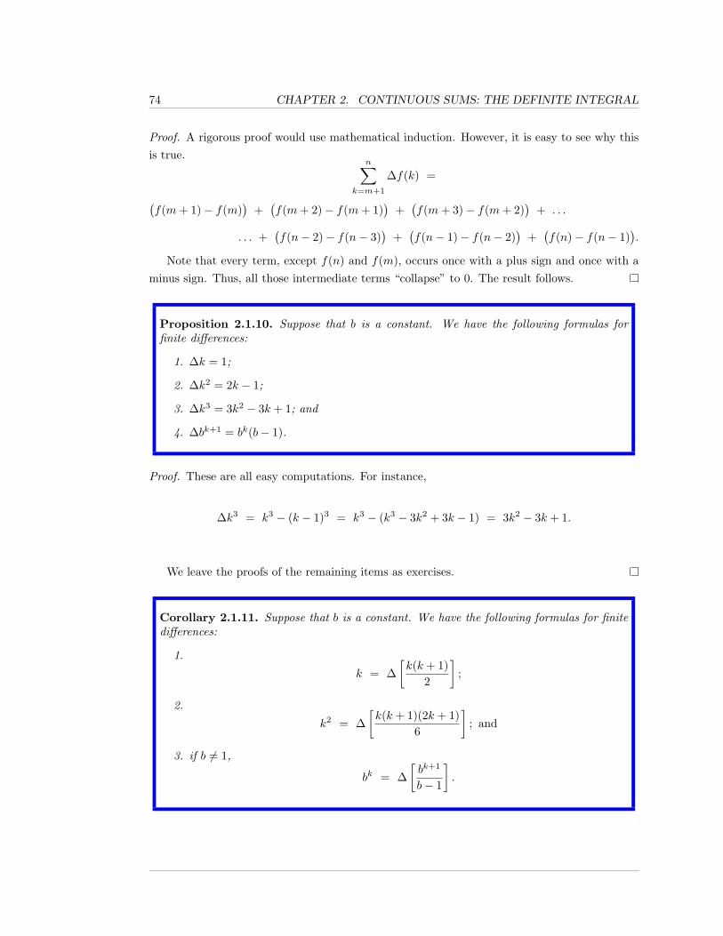
74 CHAPTER 2. CONTINUOUS SUMS: THE DEFINITE INTEGRAL
Proof. A rigorous proof would use mathematical induction. However, it is easy to see why thisis true.
n∑k=m+1
∆f(k) =
(f(m+ 1)− f(m)
)+(f(m+ 2)− f(m+ 1)
)+(f(m+ 3)− f(m+ 2)
)+ . . .
. . . +(f(n− 2)− f(n− 3)
)+(f(n− 1)− f(n− 2)
)+(f(n)− f(n− 1)
).
Note that every term, except f(n) and f(m), occurs once with a plus sign and once with aminus sign. Thus, all those intermediate terms “collapse” to 0. The result follows.
Proposition 2.1.10. Suppose that b is a constant. We have the following formulas forfinite differences:
1. ∆k = 1;
2. ∆k2 = 2k − 1;
3. ∆k3 = 3k2 − 3k + 1; and
4. ∆bk+1 = bk(b− 1).
Proof. These are all easy computations. For instance,
∆k3 = k3 − (k − 1)3 = k3 − (k3 − 3k2 + 3k − 1) = 3k2 − 3k + 1.
We leave the proofs of the remaining items as exercises.
Corollary 2.1.11. Suppose that b is a constant. We have the following formulas for finitedifferences:
1.
k = ∆[k(k + 1)
2
];
2.
k2 = ∆[k(k + 1)(2k + 1)
6
]; and
3. if b 6= 1,
bk = ∆[bk+1
b− 1
].
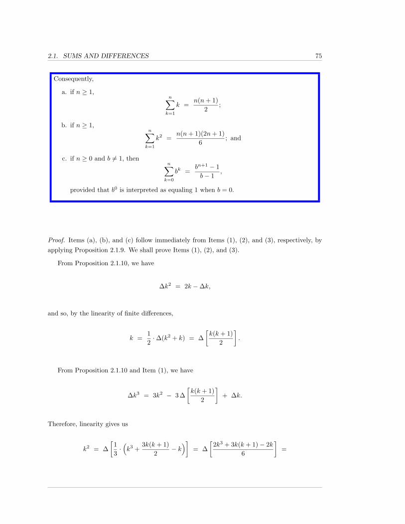
2.1. SUMS AND DIFFERENCES 75
Consequently,
a. if n ≥ 1,n∑k=1
k =n(n+ 1)
2;
b. if n ≥ 1,n∑k=1
k2 =n(n+ 1)(2n+ 1)
6; and
c. if n ≥ 0 and b 6= 1, thenn∑k=0
bk =bn+1 − 1b− 1
,
provided that b0 is interpreted as equaling 1 when b = 0.
Proof. Items (a), (b), and (c) follow immediately from Items (1), (2), and (3), respectively, byapplying Proposition 2.1.9. We shall prove Items (1), (2), and (3).
From Proposition 2.1.10, we have
∆k2 = 2k −∆k,
and so, by the linearity of finite differences,
k =12·∆(k2 + k) = ∆
[k(k + 1)
2
].
From Proposition 2.1.10 and Item (1), we have
∆k3 = 3k2 − 3 ∆[k(k + 1)
2
]+ ∆k.
Therefore, linearity gives us
k2 = ∆[
13·(k3 +
3k(k + 1)2
− k)]
= ∆[
2k3 + 3k(k + 1)− 2k6
]=
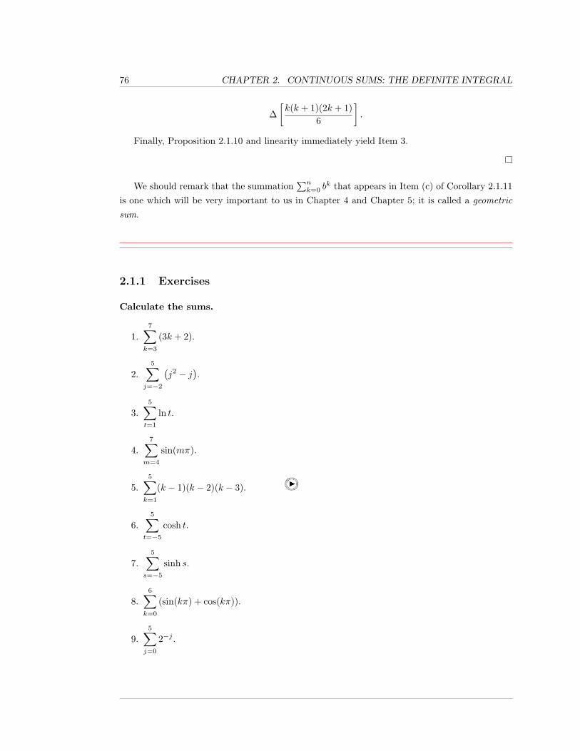
76 CHAPTER 2. CONTINUOUS SUMS: THE DEFINITE INTEGRAL
∆[k(k + 1)(2k + 1)
6
].
Finally, Proposition 2.1.10 and linearity immediately yield Item 3.
We should remark that the summation∑nk=0 b
k that appears in Item (c) of Corollary 2.1.11is one which will be very important to us in Chapter 4 and Chapter 5; it is called a geometricsum.
2.1.1 Exercises
Calculate the sums.
1.7∑k=3
(3k + 2).
2.5∑
j=−2
(j2 − j
).
3.5∑t=1
ln t.
4.7∑
m=4
sin(mπ).
5.5∑k=1
(k − 1)(k − 2)(k − 3).
6.5∑
t=−5
cosh t.
7.5∑
s=−5
sinh s.
8.6∑k=0
(sin(kπ) + cos(kπ)).
9.5∑j=0
2−j .
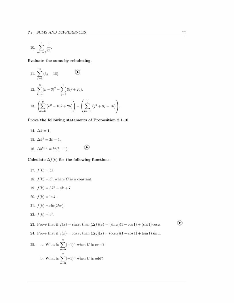
2.1. SUMS AND DIFFERENCES 77
10.3∑
m=−2
1m
.
Evaluate the sums by reindexing.
11.12∑j=6
(3j − 18).
12.8∑k=4
(k − 3)2 −5∑j=1
(9j + 20).
13.
(9∑k=6
(k2 − 10k + 25
))−
0∑j=−3
(j2 + 8j + 16
).
Prove the following statements of Proposition 2.1.10
14. ∆k = 1.
15. ∆k2 = 2k − 1.
16. ∆bk+1 = bk(b− 1).
Calculate ∆f(k) for the following functions.
17. f(k) = 5k
18. f(k) = C, where C is a constant.
19. f(k) = 3k2 − 4k + 7.
20. f(k) = ln k.
21. f(k) = sin(2kπ).
22. f(k) = 3k.
23. Prove that if f(x) = sinx, then (∆f)(x) = (sinx)(1− cos 1) + (sin 1) cosx.
24. Prove that if g(x) = cosx, then (∆g)(x) = (cosx)(1− cos 1) + (sin 1) sinx.
25. a. What isU∑n=0
(−1)n when U is even?
b. What isU∑n=0
(−1)n when U is odd?
78 CHAPTER 2. CONTINUOUS SUMS: THE DEFINITE INTEGRAL
26. Is the following statement true? Assume f and g are differentiable functions.
3∑j=1
f(j)
3∑j=1
g(j)
=3∑j=1
f(j)g(j)
Prove or give a counterexample.
27. What is100∑k=1
1k(k + 1)
? Hint: use partial fractions and find a telescoping sum.
28. What isJ∑
k=−J
f(k) if f is an odd function, f(0) = y0, and J is some positive integer?
29. What is25∑j=17
(√j −
√j − 1
)?
30. Suppose that f is a differentiable function. Prove that there exist numbers ci in each openinterval (i− 1, i), for i = 1, 2, 3, such that f(3)− f(0) = f ′(c1) + f ′(c2) + f ′(c3).
31. Recall that the average of n numbers is given by the formula:
x =∑ni=1 x
n.
Prove thatn∑i=1
(x− x) = 0.
The sample standard deviation of a data set, s, measures how spread out a data
set is. For example, if A = {84, 84, 84} and B = {80, 84, 88}, then the sample standard
deviation of B will be larger than the sample standard deviation of A since there the
points of B are more dispersed than those in set A. The sample standard deviation
of a set with n data points is
s =
√√√√ 1n− 1
n∑i=1
(x− x)2.
The units of s are the same as those of the data.
2.1. SUMS AND DIFFERENCES 79
32. A Calculus test is given to two sections of students. The grades of the students in section Aare {85, 65, 73, 40, 64, 90} and the grades of the students in section B are {84, 90, 96, 88, 100}.What are sA and sB?
33. Suppose that the week-to-week changes in a stock’s price, in dollars per share, over a sixweek period are: {+2.5,+4,−7, 0,+3}. What is s for this set? The standard deviation ofa stock’s price measures the volatility of the stock.
34. The recorded annual rainfall, in inches, for a city over a five year span is {23, 47, 35, 42, 29}.What is the sample standard deviation?
35. We define the sample variance to be the square of the sample standard deviation:
s2 =∑ni=1(xi − x)2
n− 1.
Prove the following useful alternative formula:
s2 =
(∑x2i
)− (1/n) (
∑xi)
2
(n− 1).
All sums are taken from 1 to n where n is the number of items in the data set.
Oftentimes statistics are used to measure the relationship between two variables.
For example, researchers could be interested in the relationship between drug
dosage and cancer cell counts. Basketball executives may be interested in the
relationship between a team’s free throw percentage, and the team’s overall win-
ning percentage. The linear correlation coefficient, r, quantifies the relationship.
Specifically, r helps answer the question: to what extant are the two variables lin-
early related? r is always between −1 and +1. If r is close to +1 (resp. −1), then
a strong positive (resp. negative) linear relationship exists between the variables
in the sense that as one variable increases, the second variable tends to increase
(resp. decrease) proportionally. If xi and yi are two data sets with means x and y
and standard deviations sx and sy, then r is given by:
r =∑ni=1(xi − x)(yi − y)
(n− 1)sxsy.
36. Suppose you work for a large retail store and your manager asks you study the rela-
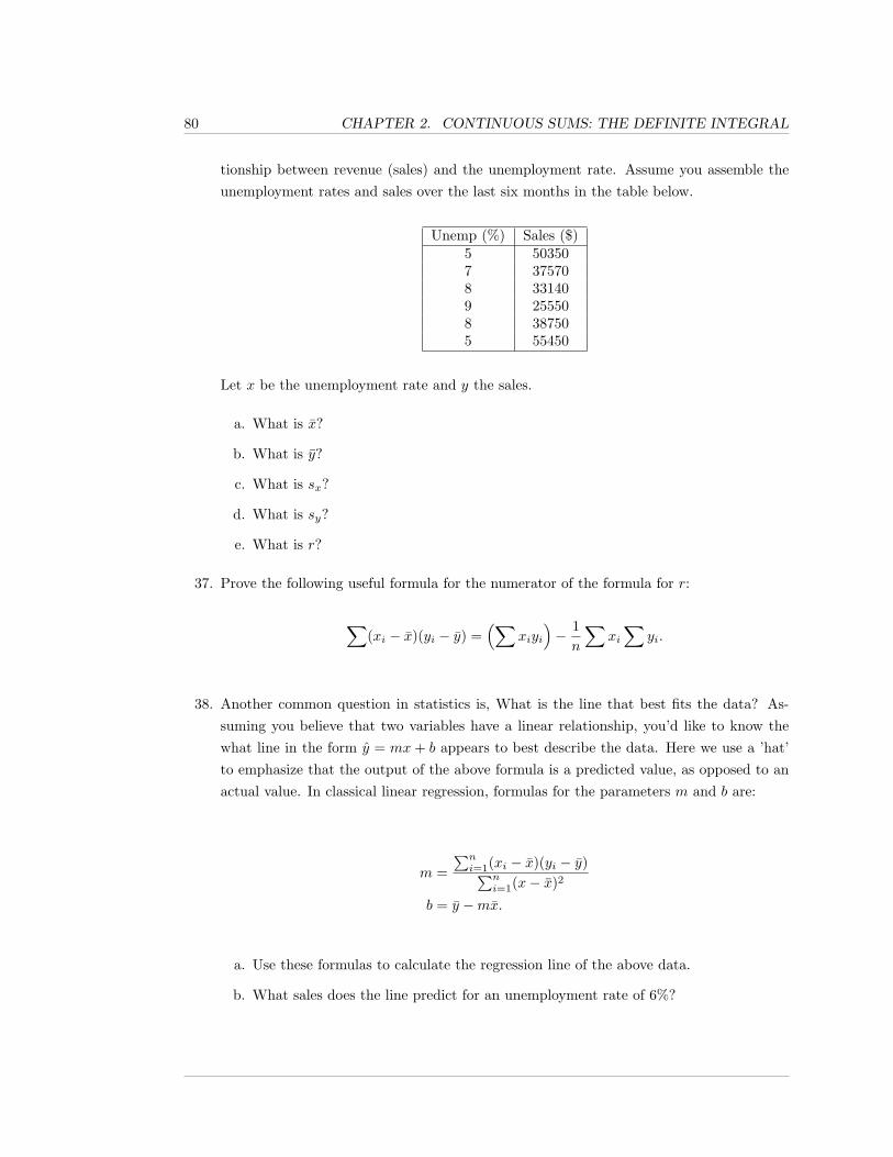
80 CHAPTER 2. CONTINUOUS SUMS: THE DEFINITE INTEGRAL
tionship between revenue (sales) and the unemployment rate. Assume you assemble theunemployment rates and sales over the last six months in the table below.
Unemp (%) Sales ($)5 503507 375708 331409 255508 387505 55450
Let x be the unemployment rate and y the sales.
a. What is x?
b. What is y?
c. What is sx?
d. What is sy?
e. What is r?
37. Prove the following useful formula for the numerator of the formula for r:
∑(xi − x)(yi − y) =
(∑xiyi
)− 1n
∑xi∑
yi.
38. Another common question in statistics is, What is the line that best fits the data? As-suming you believe that two variables have a linear relationship, you’d like to know thewhat line in the form y = mx + b appears to best describe the data. Here we use a ’hat’to emphasize that the output of the above formula is a predicted value, as opposed to anactual value. In classical linear regression, formulas for the parameters m and b are:
m =∑ni=1(xi − x)(yi − y)∑n
i=1(x− x)2
b = y −mx.
a. Use these formulas to calculate the regression line of the above data.
b. What sales does the line predict for an unemployment rate of 6%?
2.1. SUMS AND DIFFERENCES 81
Linear Regression FAQ
You probably have three good questions now:
Q In what sense is this the line of best fit?
A The line of best fit should be ’close’ to the data. We quantify closeness by the squareof the difference between the predicted and actual data. More specifically, the quantity∑
(y − y)2 is minimized.
Q Where do the formulas for m and b come from?
A We find m and b by minimizing the function:
f(m, b) =∑
(y − y)2 =∑
(mx+ b− y)2.
This is an elementary exercise in multivariable Calculus. In single variable Calculus, wefind minima of a function by locating points where the derivative is zero. This procedurehas a natural analog in higher dimensions.
Q When is it appropriate to use linear regression?
A There are several very important technical assumptions lurking behind linear regressionthat are seldom checked. One of these assumptions is that the data should be normallydistributed about its mean at each y value. Many important economic models, includingthe Capital Asset Pricing Model and the Nobel Prize winning Black-Scholes option pricingmethod rely on the normality assumption. The extremely non-normal market fluctuationssparked by the burst of the housing market bubble in 2008-2009 has caused many peopleto question the validity of the normality assumption.
Exercises 39 - 43 are based on the lyrics of the song The Twelve Days of Christ-
mas. You may find it helpful to have the lyrics in hand.
39. Let f(m) be the total number of gifts received on the mth day. On the third day ofChristmas, for example, a total of six gifts are given. Three french hens, two turtle doves,and a partridge in a pair tree. Write a formula for f(m) using summation notation.
40. What is f(12)?
82 CHAPTER 2. CONTINUOUS SUMS: THE DEFINITE INTEGRAL
41. The cumulative number of gifts received after m days, call this function F (m), is alsogrowing. By the end of the third day, for example, 10 gifts have been received: 6 fromthe 3rd day, 3 from the 2nd day and 1 from the 1st day. Express F (m) using summationnotation.
42. What is F (12)?
43. Research the terms triangular numbers and tetrahedral numbers on the internet. How dothese terms relate to these exercises?
44. By how much does ln 2 differ from4∑
n=1
(−1)n−1
n? Does the summation get closer to ln 2 if
the upper limit is changed from 4 to 5?
45. Let An =n∑u=1
(u2 + 1
2
)2
and Bn =n∑u=1
(u2 − 1
2
)2
. Find an expression for An + Bn.
Hint: combine the sums immediately rather than dealing with each one individually.
The Fibonacci sequence is defined recursively. Set F0 = 0, F1 = 1 and, for k ≥ 2,
Fk = Fk−1 +Fk−2. This gives a sequence {0, 1, 1, 2, 3, 5, 8, ...}. Prove the following facts
about the Fibonacci sequence.
46. ∆Fk = Fk−2.
47.2n∑k=0
Fk = F2n+2 − 1.
48.n∑k=1
F2k−1 = F2n.
49.n∑k=0
F2k = F2n+1 − 1.
50.n∑k=0
F 2k = FnFn+1.
2.2. PRELUDE TO THE DEFINITE INTEGRAL 83
2.2 Prelude to the Definite Integral:Riemann Sums
In differential Calculus, the instantaneous rate of change of a function is defined as follows: wehave a notion of the average rate of change of the function, and we believe, for small changesin the independent variable, that the average rate of change approximates something. Wethen take limits of the average rates of change to define the instantaneous rate of change, thederivative.
In this section, we do something analogous: we will define Riemann sums, which are supposedto be approximations to “continuous sums of an infinite number of infinitesimal contributions”.As with the passage from average rates of change to instantaneous ones, we pass from Riemannsums to continuous sums by taking limits. The continuous sum that we end up with is calledthe definite integral.
Let’s begin with an extended example.
Example 2.2.1. Suppose that a car is traveling along a straight road, on which a coordinateaxis has been laid out in meters. Let p(t) denote the position of the car (on the axis), at time tseconds (after some initial starting time), and let v(t) denote the velocity of the car, in metersper second, at time t seconds.
If the driver of the car were to brake hard, or step down hard on the accelerator, he or shecould easily change the velocity of the car by a noticeable amount in 2 seconds. However, itwould be difficult to change the velocity of the car in a significant way in a substantially smallertime interval, like 0.25 seconds.
We want to discuss how you would estimate the change in the position, the displacement, ofthe car, between times 0 and 2 seconds, if you were given some velocity measurements. First,we should clarify that, when we have two numbers a and b, where a < b, and we write that xis between a and b, we mean to allow for the possibility that x equals a or b, i.e., “x is betweena and b” means a ≤ x ≤ b. If a < b, and we write that x is strictly between a and b, we meanto disallow the possibility that x equals a or b, i.e., “x is strictly between a and b” meansa < x < b.
Now, suppose that we know that,
• at some time between 0 and 0.3 seconds, the car is moving with velocity 30 m/s;
84 CHAPTER 2. CONTINUOUS SUMS: THE DEFINITE INTEGRAL
• at some time between 0.3 and 0.8 seconds, the car is moving with velocity 20 m/s;
• at some time between 0.8 and 1.2 seconds, the car is moving with velocity 10 m/s; and,
• at some time between 1.2 and 2 seconds, the car is moving at −2 m/s (i.e., at 2 m/s in thenegative direction).
How can we estimate the displacement of the car between times t = 0 and t = 2 seconds, i.e.,how can we estimate p(2)− p(0)?
Note that we have the equalityp(2)− p(0) = (2.2)(
p(2)− p(1.2))
+(p(1.2)− p(0.8)
)+(p(0.8)− p(0.3)
)+(p(0.3)− p(0)
),
which results from the fact that all of the terms, other than p(2) and p(0), cancel out, that is,the sum telescopes, as in Proposition 2.1.9. Thus, to estimate p(2)− p(0), we can estimate thefour sub-displacements appearing in Formula 2.2, and add them together.
Okay. Fine. So how do we approximate each of the sub-displacements?
The answer is that, for each of the four intervals of time [0, 0.3], [0.3, 0.8], [0.8, 1.2], and[1.2, 2] (subintervals of [0, 2]), we use, as an approximation, that the velocity is constant onthe given interval. Why do we do this? For two reasons. First, the subintervals of time arefairly small, small enough so that we believe that the velocity cannot change too much on eachsubinterval. Second, we don’t really have much of a choice, considering that the only data thatwe are given is the velocity at some time in each of the given subintervals.
Thus, as an approximation, we assume/pretend that, on the subintervals [0, 0.3], [0.3, 0.8],[0.8, 1.2], and [1.2, 2], the velocity is constantly 30, 20, 10, and −2 m/s, respectively. Now, if thevelocity is a constant during an interval of time, then that velocity is also the average velocityduring the interval of time, and we know that the average velocity on an interval of time is thechange in position on the interval divided by the change in time on the interval. Thus, we havethe four approximations (in m/s):
p(2)− p(1.2)2− 1.2
≈ −2,p(1.2)− p(0.8)
1.2− 0.8≈ 10,
p(0.8)− p(0.3)0.8− 0.3
≈ 20, and
p(0.3)− p(0)0.3− 0
≈ 30.
Therefore, we approximate that the displacement of the car, between times t = 0 and t = 2seconds:
p(2)− p(0) =
2.2. PRELUDE TO THE DEFINITE INTEGRAL 85
(p(2)− p(1.2)
)+(p(1.2)− p(0.8)
)+(p(0.8)− p(0.3)
)+(p(0.3)− p(0)
)≈
−2(2− 1.2) + 10(1.2− 0.8) + 20(0.8− 0.3) + 30(0.3− 0) =
−1.6 + 4 + 10 + 9 = 21.4 meters.
Therefore, we conclude that the displacement of the car, between times t = 0 and t = 2 seconds,is approximately 21.4 meters. Note that this is an estimate of the change in the position; wecannot estimate (in a reasonable manner) the actual position of the car at t = 2 seconds, unlesswe have p(0) (or, at least, an estimate of p(0)).
Our data and approximations of the displacements on the subintervals look best in a table.
subinterval (sec.) [0, 0.3] [0.3, 0.8] [0.8, 1.2] [1.2, 2]
time (sec.) t1 t2 t3 t4
velocity (m/s) 30 20 10 -2
Approx. ∆p (meters) 9 10 4 -1.6
Approx. total ∆p = 9 + 10 + 4 + (−1.6) = 21.4 meters.
Note that we gave the names t1, t2, t3, and t4 to the times in the corresponding subintervalsat which we were given the velocities that appear in the 3rd row. Our approximation of thetotal displacement is the sum of the entries in the 4th row of the table.
How could we obtain a better approximation of the displacement p(2) − p(0) or, at least,an approximation that we’d expect to be better? We could subdivide the subintervals aboveinto even smaller subintervals of time, and be given velocities at some time in each of the newsubintervals.
For instance, if we thought that 0.8 seconds was too large of a change in time over whichto approximate the velocity as being constant, we might subdivide the last subinterval [1.2, 2]above into two subintervals, say [1.2, 1.6] and [1.6, 2]. We would then need to know which ofthese new subintervals contains the time t4 (both would, if t4 = 1.6), and we’d need to be giventhe velocity at some time in the other new subinterval. For this example, let’s assume that t4 isin the subinterval [1.2, 1.6], and that we know, at some time t5 in the interval [1.6, 2], that thevelocity is −5 m/s. What approximation do we get for the total displacement now?
Our new table is:
subinterval (sec.) [0, 0.3] [0.3, 0.8] [0.8, 1.2] [1.2, 1.6] [1.6, 2]
time (sec.) t1 t2 t3 t4 t5
velocity (m/s) 30 20 10 -2 -5
Approx. ∆p (meters) 9 10 4 -0.8 -2
Approx. total ∆p = 9 + 10 + 4 + (−0.8) + (−2) = 20.2 meters.
86 CHAPTER 2. CONTINUOUS SUMS: THE DEFINITE INTEGRAL
Our new approximation for the displacement p(2)−p(0) is no longer 21.4 meters, but is now20.2 meters.
Do we really know that this new approximation is better than the first one? Not really. Forall we know, in the last subinterval [1.6, 2], the velocity is actually closer to −2 m/s mostof time, and is only close to −5 m/s for a tiny subinterval around t5. We can try to appealto our intuition and/or physical experience to say that, in 0.4 seconds, the velocity cannotchange a significant amount, but that’s no proof, and it also leaves us with the question of:what’s a “significant” amount? Nonetheless, we “suspect” that subdividing our subintervalsinto smaller subintervals leads to better approximations, provided we take our subdivisionssmall enough.
Despite the remark/warning above, it is nonetheless true that there is a strong sense in whichusing small enough subintervals guarantees a close approximation; see the remark below.
Remark 2.2.2. It is possible to make precise in what way the approximation “gets better”as the time intervals get smaller. First, we need to assume that the velocity function v(t)is continuous on the interval [0, 2]. Now, call a subdivision of the interval [0, 2] into a finitecollection of subintervals a partition of [0, 2] (technically, the partition is just the set of endpointsof the subintervals; see Definition 2.2.3). Call the length of the longest (any one of the longest)subintervals the mesh of the partition. Thus, if the mesh of the partition is less than some (small)positive constant δ, then every subinterval in the partition has length less than δ; informally,this means that saying that the mesh of a partition is small implies that every subinterval inthe partition is small.
Now, we can state carefully in what sense picking small subintervals of time, and being giventhe velocity at one time per time interval, allows you to accurately approximate the actualdisplacement. Given any ε > 0 (think: ε could be an arbitrarily small positive number), we canguarantee that our approximation for the displacement is within ε of the actual displacementby using partitions with a small enough mesh, i.e., there exists a number δ > 0 such that, forevery partition of [0, 2], with mesh less than δ, for every choice of one time (a sample point) persubinterval at which to be given the velocity, the sum of the products of the lengths of eachsubinterval with the given velocities for the subintervals will be within ε of the displacementp(2)− p(0).
The above statement is a result of the definition of the definite integral, Definition 2.3.1,Theorem 2.3.8, and the Fundamental Theorem of Calculus, Theorem 2.4.10.
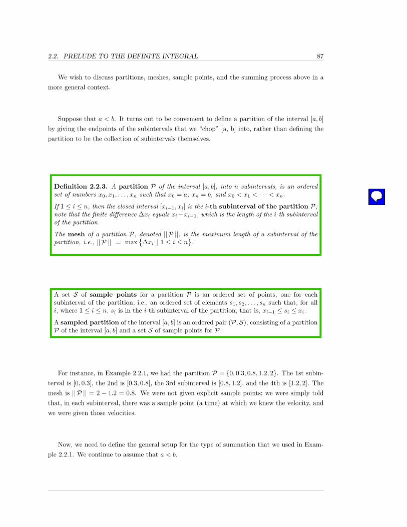
2.2. PRELUDE TO THE DEFINITE INTEGRAL 87
We wish to discuss partitions, meshes, sample points, and the summing process above in amore general context.
Suppose that a < b. It turns out to be convenient to define a partition of the interval [a, b]by giving the endpoints of the subintervals that we “chop” [a, b] into, rather than defining thepartition to be the collection of subintervals themselves.
Definition 2.2.3. A partition P of the interval [a, b], into n subintervals, is an orderedset of numbers x0, x1, . . . , xn such that x0 = a, xn = b, and x0 < x1 < · · · < xn.
If 1 ≤ i ≤ n, then the closed interval [xi−1, xi] is the i-th subinterval of the partition P;note that the finite difference ∆xi equals xi−xi−1, which is the length of the i-th subintervalof the partition.
The mesh of a partition P, denoted || P ||, is the maximum length of a subinterval of thepartition, i.e., || P || = max
{∆xi | 1 ≤ i ≤ n
}.
A set S of sample points for a partition P is an ordered set of points, one for eachsubinterval of the partition, i.e., an ordered set of elements s1, s2, . . . , sn such that, for alli, where 1 ≤ i ≤ n, si is in the i-th subinterval of the partition, that is, xi−1 ≤ si ≤ xi.
A sampled partition of the interval [a, b] is an ordered pair (P,S), consisting of a partitionP of the interval [a, b] and a set S of sample points for P.
For instance, in Example 2.2.1, we had the partition P = {0, 0.3, 0.8, 1.2, 2}. The 1st subin-terval is [0, 0.3], the 2nd is [0.3, 0.8], the 3rd subinterval is [0.8, 1.2], and the 4th is [1.2, 2]. Themesh is || P || = 2 − 1.2 = 0.8. We were not given explicit sample points; we were simply toldthat, in each subinterval, there was a sample point (a time) at which we knew the velocity, andwe were given those velocities.
Now, we need to define the general setup for the type of summation that we used in Exam-ple 2.2.1. We continue to assume that a < b.
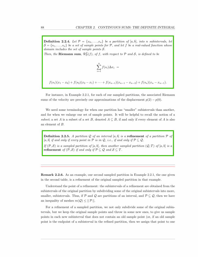
88 CHAPTER 2. CONTINUOUS SUMS: THE DEFINITE INTEGRAL
Definition 2.2.4. Let P = {x0, . . . , xn} be a partition of [a, b], into n subintervals, letS = {s1, . . . , sn} be a set of sample points for P, and let f be a real-valued function whosedomain includes the set of sample points S.Then, the Riemann sum, RSP(f), of f , with respect to P and S, is defined to be
n∑i=1
f(si)∆xi =
f(s1)(x1 − x0) + f(s2)(x2 − x1) + · · ·+ f(xn−1)(xn−1 − xn−2) + f(sn)(xn − xn−1).
For instance, in Example 2.2.1, for each of our sampled partitions, the associated Riemannsums of the velocity are precisely our approximations of the displacement p(2)− p(0).
We need some terminology for when one partition has “smaller” subintervals than another,and for when we enlarge our set of sample points. It will be helpful to recall the notion of asubset; a set A is a subset of a set B, denoted A ⊆ B, if and only if every element of A is alsoan element of B.
Definition 2.2.5. A partition Q of an interval [a, b] is a refinement of a partition P of[a, b] if and only if every point in P is in Q, i.e., if and only if P ⊆ Q.
If (P,S) is a sampled partition of [a, b], then another sampled partition (Q, T ) of [a, b] is arefinement of (P,S) if and only if P ⊆ Q and S ⊆ T .
Remark 2.2.6. As an example, our second sampled partition in Example 2.2.1, the one givenin the second table, is a refinement of the original sampled partition in that example.
Understand the point of a refinement: the subintervals of a refinement are obtained from thesubintervals of the original partition by subdividing some of the original subintervals into more,smaller, subintervals. Thus, if P and Q are partitions of an interval, and P ⊆ Q, then we havean inequality of meshes m(Q) ≤ || P ||.
For a refinement of a sampled partition, we not only subdivide some of the original subin-tervals, but we keep the original sample points and throw in some new ones, to give us samplepoints in each new subinterval that does not contain an old sample point (or, if an old samplepoint is the endpoint of a subinterval in the refined partition, then we assign that point to one
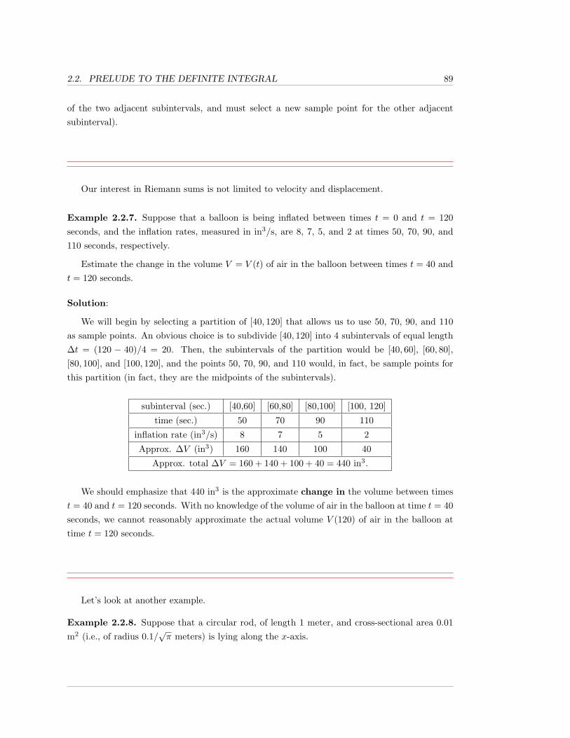
2.2. PRELUDE TO THE DEFINITE INTEGRAL 89
of the two adjacent subintervals, and must select a new sample point for the other adjacentsubinterval).
Our interest in Riemann sums is not limited to velocity and displacement.
Example 2.2.7. Suppose that a balloon is being inflated between times t = 0 and t = 120seconds, and the inflation rates, measured in in3/s, are 8, 7, 5, and 2 at times 50, 70, 90, and110 seconds, respectively.
Estimate the change in the volume V = V (t) of air in the balloon between times t = 40 andt = 120 seconds.
Solution:
We will begin by selecting a partition of [40, 120] that allows us to use 50, 70, 90, and 110as sample points. An obvious choice is to subdivide [40, 120] into 4 subintervals of equal length∆t = (120 − 40)/4 = 20. Then, the subintervals of the partition would be [40, 60], [60, 80],[80, 100], and [100, 120], and the points 50, 70, 90, and 110 would, in fact, be sample points forthis partition (in fact, they are the midpoints of the subintervals).
subinterval (sec.) [40,60] [60,80] [80,100] [100, 120]
time (sec.) 50 70 90 110
inflation rate (in3/s) 8 7 5 2
Approx. ∆V (in3) 160 140 100 40
Approx. total ∆V = 160 + 140 + 100 + 40 = 440 in3.
We should emphasize that 440 in3 is the approximate change in the volume between timest = 40 and t = 120 seconds. With no knowledge of the volume of air in the balloon at time t = 40seconds, we cannot reasonably approximate the actual volume V (120) of air in the balloon attime t = 120 seconds.
Let’s look at another example.
Example 2.2.8. Suppose that a circular rod, of length 1 meter, and cross-sectional area 0.01m2 (i.e., of radius 0.1/
√π meters) is lying along the x-axis.
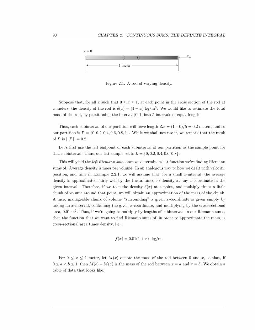
90 CHAPTER 2. CONTINUOUS SUMS: THE DEFINITE INTEGRAL
Figure 2.1: A rod of varying density.
Suppose that, for all x such that 0 ≤ x ≤ 1, at each point in the cross section of the rod atx meters, the density of the rod is δ(x) = (1 + x) kg/m3. We would like to estimate the totalmass of the rod, by partitioning the interval [0, 1] into 5 intervals of equal length.
Thus, each subinterval of our partition will have length ∆x = (1− 0)/5 = 0.2 meters, and soour partition is P = {0, 0.2, 0.4, 0.6, 0.8, 1}. While we shall not use it, we remark that the meshof P is || P || = 0.2.
Let’s first use the left endpoint of each subinterval of our partition as the sample point forthat subinterval. Thus, our left sample set is L = {0, 0.2, 0.4, 0.6, 0.8}.
This will yield the left Riemann sum, once we determine what function we’re finding Riemannsums of. Average density is mass per volume. In an analogous way to how we dealt with velocity,position, and time in Example 2.2.1, we will assume that, for a small x-interval, the averagedensity is approximated fairly well by the (instantaneous) density at any x-coordinate in thegiven interval. Therefore, if we take the density δ(x) at a point, and multiply times a littlechunk of volume around that point, we will obtain an approximation of the mass of the chunk.A nice, manageable chunk of volume “surrounding” a given x-coordinate is given simply bytaking an x-interval, containing the given x-coordinate, and multiplying by the cross-sectionalarea, 0.01 m2. Thus, if we’re going to multiply by lengths of subintervals in our Riemann sums,then the function that we want to find Riemann sums of, in order to approximate the mass, iscross-sectional area times density, i.e.,
f(x) = 0.01(1 + x) kg/m.
For 0 ≤ x ≤ 1 meter, let M(x) denote the mass of the rod between 0 and x, so that, if0 ≤ a < b ≤ 1, then M(b)−M(a) is the mass of the rod between x = a and x = b. We obtain atable of data that looks like:
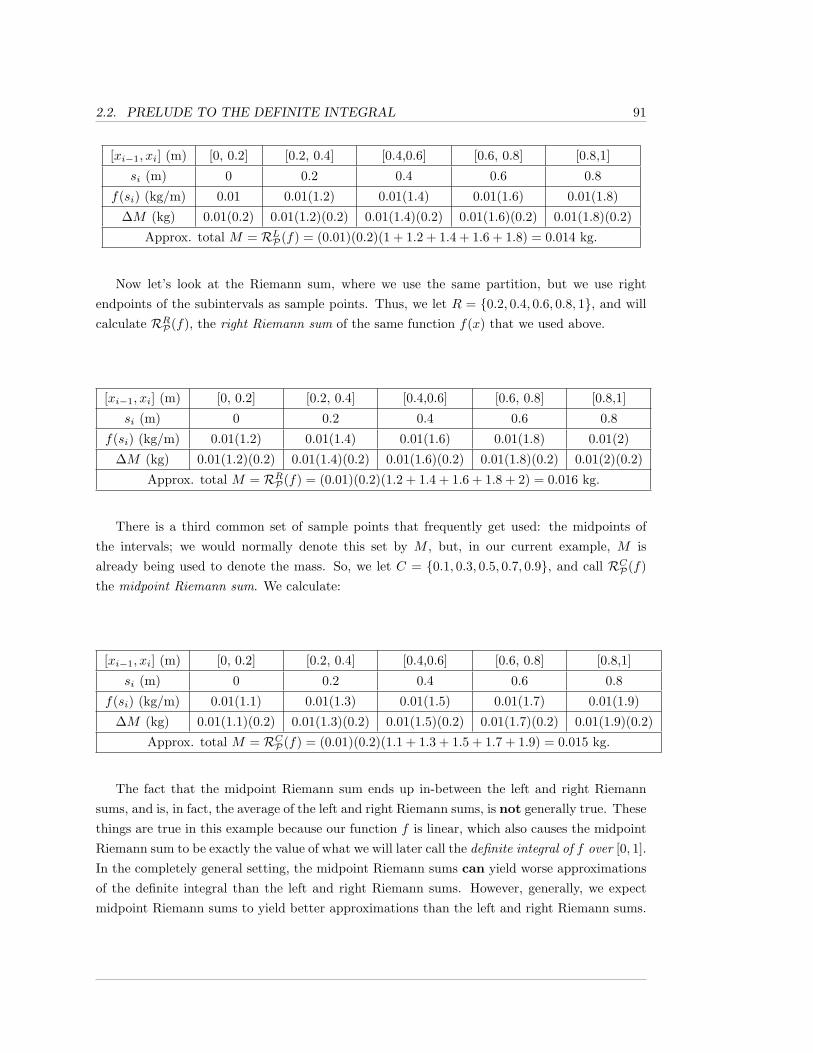
2.2. PRELUDE TO THE DEFINITE INTEGRAL 91
[xi−1, xi] (m) [0, 0.2] [0.2, 0.4] [0.4,0.6] [0.6, 0.8] [0.8,1]
si (m) 0 0.2 0.4 0.6 0.8
f(si) (kg/m) 0.01 0.01(1.2) 0.01(1.4) 0.01(1.6) 0.01(1.8)
∆M (kg) 0.01(0.2) 0.01(1.2)(0.2) 0.01(1.4)(0.2) 0.01(1.6)(0.2) 0.01(1.8)(0.2)
Approx. total M = RLP(f) = (0.01)(0.2)(1 + 1.2 + 1.4 + 1.6 + 1.8) = 0.014 kg.
Now let’s look at the Riemann sum, where we use the same partition, but we use rightendpoints of the subintervals as sample points. Thus, we let R = {0.2, 0.4, 0.6, 0.8, 1}, and willcalculate RRP(f), the right Riemann sum of the same function f(x) that we used above.
[xi−1, xi] (m) [0, 0.2] [0.2, 0.4] [0.4,0.6] [0.6, 0.8] [0.8,1]
si (m) 0 0.2 0.4 0.6 0.8
f(si) (kg/m) 0.01(1.2) 0.01(1.4) 0.01(1.6) 0.01(1.8) 0.01(2)
∆M (kg) 0.01(1.2)(0.2) 0.01(1.4)(0.2) 0.01(1.6)(0.2) 0.01(1.8)(0.2) 0.01(2)(0.2)
Approx. total M = RRP(f) = (0.01)(0.2)(1.2 + 1.4 + 1.6 + 1.8 + 2) = 0.016 kg.
There is a third common set of sample points that frequently get used: the midpoints ofthe intervals; we would normally denote this set by M , but, in our current example, M isalready being used to denote the mass. So, we let C = {0.1, 0.3, 0.5, 0.7, 0.9}, and call RCP(f)the midpoint Riemann sum. We calculate:
[xi−1, xi] (m) [0, 0.2] [0.2, 0.4] [0.4,0.6] [0.6, 0.8] [0.8,1]
si (m) 0 0.2 0.4 0.6 0.8
f(si) (kg/m) 0.01(1.1) 0.01(1.3) 0.01(1.5) 0.01(1.7) 0.01(1.9)
∆M (kg) 0.01(1.1)(0.2) 0.01(1.3)(0.2) 0.01(1.5)(0.2) 0.01(1.7)(0.2) 0.01(1.9)(0.2)
Approx. total M = RCP(f) = (0.01)(0.2)(1.1 + 1.3 + 1.5 + 1.7 + 1.9) = 0.015 kg.
The fact that the midpoint Riemann sum ends up in-between the left and right Riemannsums, and is, in fact, the average of the left and right Riemann sums, is not generally true. Thesethings are true in this example because our function f is linear, which also causes the midpointRiemann sum to be exactly the value of what we will later call the definite integral of f over [0, 1].In the completely general setting, the midpoint Riemann sums can yield worse approximationsof the definite integral than the left and right Riemann sums. However, generally, we expectmidpoint Riemann sums to yield better approximations than the left and right Riemann sums.
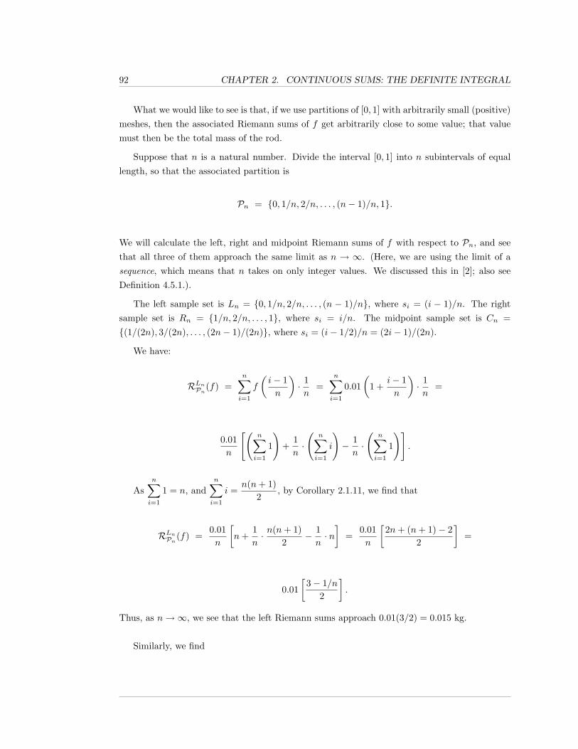
92 CHAPTER 2. CONTINUOUS SUMS: THE DEFINITE INTEGRAL
What we would like to see is that, if we use partitions of [0, 1] with arbitrarily small (positive)meshes, then the associated Riemann sums of f get arbitrarily close to some value; that valuemust then be the total mass of the rod.
Suppose that n is a natural number. Divide the interval [0, 1] into n subintervals of equallength, so that the associated partition is
Pn = {0, 1/n, 2/n, . . . , (n− 1)/n, 1}.
We will calculate the left, right and midpoint Riemann sums of f with respect to Pn, and seethat all three of them approach the same limit as n → ∞. (Here, we are using the limit of asequence, which means that n takes on only integer values. We discussed this in [2]; also seeDefinition 4.5.1.).
The left sample set is Ln = {0, 1/n, 2/n, . . . , (n − 1)/n}, where si = (i − 1)/n. The rightsample set is Rn = {1/n, 2/n, . . . , 1}, where si = i/n. The midpoint sample set is Cn ={(1/(2n), 3/(2n), . . . , (2n− 1)/(2n)}, where si = (i− 1/2)/n = (2i− 1)/(2n).
We have:
RLnPn(f) =n∑i=1
f
(i− 1n
)· 1n
=n∑i=1
0.01(
1 +i− 1n
)· 1n
=
0.01n
[(n∑i=1
1
)+
1n·
(n∑i=1
i
)− 1n·
(n∑i=1
1
)].
Asn∑i=1
1 = n, andn∑i=1
i =n(n+ 1)
2, by Corollary 2.1.11, we find that
RLnPn(f) =0.01n
[n+
1n· n(n+ 1)
2− 1n· n]
=0.01n
[2n+ (n+ 1)− 2
2
]=
0.01[
3− 1/n2
].
Thus, as n→∞, we see that the left Riemann sums approach 0.01(3/2) = 0.015 kg.
Similarly, we find
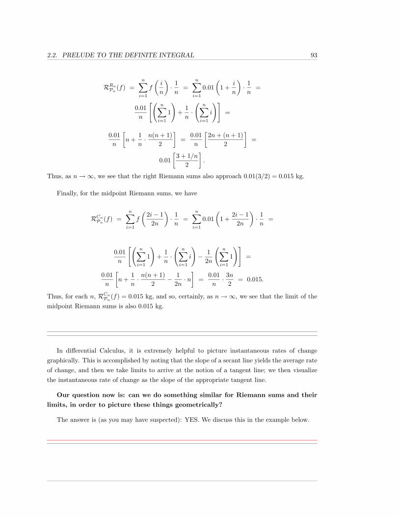
2.2. PRELUDE TO THE DEFINITE INTEGRAL 93
RRnPn (f) =n∑i=1
f
(i
n
)· 1n
=n∑i=1
0.01(
1 +i
n
)· 1n
=
0.01n
[(n∑i=1
1
)+
1n·
(n∑i=1
i
)]=
0.01n
[n+
1n· n(n+ 1)
2
]=
0.01n
[2n+ (n+ 1)
2
]=
0.01[
3 + 1/n2
].
Thus, as n→∞, we see that the right Riemann sums also approach 0.01(3/2) = 0.015 kg.
Finally, for the midpoint Riemann sums, we have
RCnPn(f) =n∑i=1
f
(2i− 1
2n
)· 1n
=n∑i=1
0.01(
1 +2i− 1
2n
)· 1n
=
0.01n
[(n∑i=1
1
)+
1n·
(n∑i=1
i
)− 1
2n
(n∑i=1
1
)]=
0.01n
[n+
1n· n(n+ 1)
2− 1
2n· n]
=0.01n· 3n
2= 0.015.
Thus, for each n, RCnPn(f) = 0.015 kg, and so, certainly, as n→∞, we see that the limit of themidpoint Riemann sums is also 0.015 kg.
In differential Calculus, it is extremely helpful to picture instantaneous rates of changegraphically. This is accomplished by noting that the slope of a secant line yields the average rateof change, and then we take limits to arrive at the notion of a tangent line; we then visualizethe instantaneous rate of change as the slope of the appropriate tangent line.
Our question now is: can we do something similar for Riemann sums and their
limits, in order to picture these things geometrically?
The answer is (as you may have suspected): YES. We discuss this in the example below.
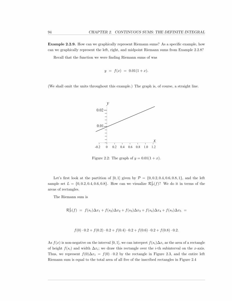
94 CHAPTER 2. CONTINUOUS SUMS: THE DEFINITE INTEGRAL
Example 2.2.9. How can we graphically represent Riemann sums? As a specific example, howcan we graphically represent the left, right, and midpoint Riemann sums from Example 2.2.8?
Recall that the function we were finding Riemann sums of was
y = f(x) = 0.01(1 + x).
(We shall omit the units throughout this example.) The graph is, of course, a straight line.
0.20-0.2 0.4 0.6 0.8 1.0 1.2x
y0.010.02
0.20-0.2 0.4 0.6 0.8 1.0 1.2x
y0.010.02
0.20-0.2 0.4 0.6 0.8 1.0 1.2x
y0.010.02
0.20-0.2 0.4 0.6 0.8 1.0 1.2x
y0.010.02
0.20-0.2 0.4 0.6 0.8 1.0 1.2x
y0.010.02
0.20-0.2 0.4 0.6 0.8 1.0 1.2x
y0.010.02
0.20-0.2 0.4 0.6 0.8 1.0 1.2x
y0.010.02
0.20-0.2 0.4 0.6 0.8 1.0 1.2x
y0.010.02
Figure 2.2: The graph of y = 0.01(1 + x).
Let’s first look at the partition of [0, 1] given by P = {0, 0.2, 0.4, 0.6, 0.8, 1}, and the leftsample set L = {0, 0.2, 0.4, 0.6, 0.8}. How can we visualize RLP(f)? We do it in terms of theareas of rectangles.
The Riemann sum is
RLP(f) = f(s1)∆x1 + f(s2)∆x2 + f(s3)∆x3 + f(s4)∆x4 + f(s5)∆x5 =
f(0) · 0.2 + f(0.2) · 0.2 + f(0.4) · 0.2 + f(0.6) · 0.2 + f(0.8) · 0.2.
As f(x) is non-negative on the interval [0, 1], we can interpret f(si)∆xi as the area of a rectangleof height f(si) and width ∆xi; we draw this rectangle over the i-th subinterval on the x-axis.Thus, we represent f(0)∆x1 = f(0) · 0.2 by the rectangle in Figure 2.3, and the entire leftRiemann sum is equal to the total area of all five of the inscribed rectangles in Figure 2.4
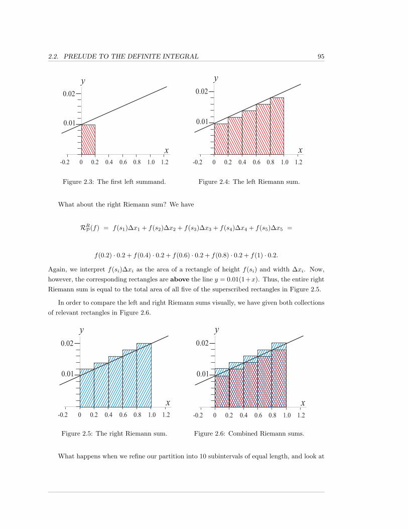
2.2. PRELUDE TO THE DEFINITE INTEGRAL 95
0.20-0.2 0.4 0.6 0.8 1.0 1.2x
y0.010.02
0.20-0.2 0.4 0.6 0.8 1.0 1.2x
y0.010.02
0.20-0.2 0.4 0.6 0.8 1.0 1.2x
y0.010.02
0.20-0.2 0.4 0.6 0.8 1.0 1.2x
y0.010.02
0.20-0.2 0.4 0.6 0.8 1.0 1.2x
y0.010.02
0.20-0.2 0.4 0.6 0.8 1.0 1.2x
y0.010.02
0.20-0.2 0.4 0.6 0.8 1.0 1.2x
y0.010.02
0.20-0.2 0.4 0.6 0.8 1.0 1.2x
y0.010.02
Figure 2.3: The first left summand.
0.20-0.2 0.4 0.6 0.8 1.0 1.2x
y0.010.02
0.20-0.2 0.4 0.6 0.8 1.0 1.2x
y0.010.02
0.20-0.2 0.4 0.6 0.8 1.0 1.2x
y0.010.02
0.20-0.2 0.4 0.6 0.8 1.0 1.2x
y0.010.02
0.20-0.2 0.4 0.6 0.8 1.0 1.2x
y0.010.02
0.20-0.2 0.4 0.6 0.8 1.0 1.2x
y0.010.02
0.20-0.2 0.4 0.6 0.8 1.0 1.2x
y0.010.02
0.20-0.2 0.4 0.6 0.8 1.0 1.2x
y0.010.02
Figure 2.4: The left Riemann sum.
What about the right Riemann sum? We have
RRP(f) = f(s1)∆x1 + f(s2)∆x2 + f(s3)∆x3 + f(s4)∆x4 + f(s5)∆x5 =
f(0.2) · 0.2 + f(0.4) · 0.2 + f(0.6) · 0.2 + f(0.8) · 0.2 + f(1) · 0.2.
Again, we interpret f(si)∆xi as the area of a rectangle of height f(si) and width ∆xi. Now,however, the corresponding rectangles are above the line y = 0.01(1+x). Thus, the entire rightRiemann sum is equal to the total area of all five of the superscribed rectangles in Figure 2.5.
In order to compare the left and right Riemann sums visually, we have given both collectionsof relevant rectangles in Figure 2.6.
0.20-0.2 0.4 0.6 0.8 1.0 1.2x
y0.010.02
0.20-0.2 0.4 0.6 0.8 1.0 1.2x
y0.010.02
0.20-0.2 0.4 0.6 0.8 1.0 1.2x
y0.010.02
0.20-0.2 0.4 0.6 0.8 1.0 1.2x
y0.010.02
0.20-0.2 0.4 0.6 0.8 1.0 1.2x
y0.010.02
0.20-0.2 0.4 0.6 0.8 1.0 1.2x
y0.010.02
0.20-0.2 0.4 0.6 0.8 1.0 1.2x
y0.010.02
0.20-0.2 0.4 0.6 0.8 1.0 1.2x
y0.010.02
Figure 2.5: The right Riemann sum.
0.20-0.2 0.4 0.6 0.8 1.0 1.2x
y0.010.02
0.20-0.2 0.4 0.6 0.8 1.0 1.2x
y0.010.02
0.20-0.2 0.4 0.6 0.8 1.0 1.2x
y0.010.02
0.20-0.2 0.4 0.6 0.8 1.0 1.2x
y0.010.02
0.20-0.2 0.4 0.6 0.8 1.0 1.2x
y0.010.02
0.20-0.2 0.4 0.6 0.8 1.0 1.2x
y0.010.02
0.20-0.2 0.4 0.6 0.8 1.0 1.2x
y0.010.02
0.20-0.2 0.4 0.6 0.8 1.0 1.2x
y0.010.02Figure 2.6: Combined Riemann sums.
What happens when we refine our partition into 10 subintervals of equal length, and look at
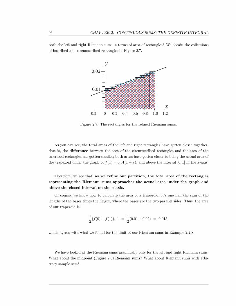
96 CHAPTER 2. CONTINUOUS SUMS: THE DEFINITE INTEGRAL
both the left and right Riemann sums in terms of area of rectangles? We obtain the collectionsof inscribed and circumscribed rectangles in Figure 2.7.
0.20-0.2 0.4 0.6 0.8 1.0 1.2x
y0.010.02
0.20-0.2 0.4 0.6 0.8 1.0 1.2x
y0.010.02
0.20-0.2 0.4 0.6 0.8 1.0 1.2x
y0.010.02
0.20-0.2 0.4 0.6 0.8 1.0 1.2x
y0.010.02
0.20-0.2 0.4 0.6 0.8 1.0 1.2x
y0.010.02
0.20-0.2 0.4 0.6 0.8 1.0 1.2x
y0.010.02
0.20-0.2 0.4 0.6 0.8 1.0 1.2x
y0.010.02
0.20-0.2 0.4 0.6 0.8 1.0 1.2x
y0.010.02
Figure 2.7: The rectangles for the refined Riemann sums.
As you can see, the total areas of the left and right rectangles have gotten closer together,that is, the difference between the area of the circumscribed rectangles and the area of theinscribed rectangles has gotten smaller; both areas have gotten closer to being the actual area ofthe trapezoid under the graph of f(x) = 0.01(1 + x), and above the interval [0, 1] in the x-axis.
Therefore, we see that, as we refine our partition, the total area of the rectangles
representing the Riemann sums approaches the actual area under the graph and
above the closed interval on the x-axis.
Of course, we know how to calculate the area of a trapezoid; it’s one half the sum of thelengths of the bases times the height, where the bases are the two parallel sides. Thus, the areaof our trapezoid is
12(f(0) + f(1)
)· 1 =
12
(0.01 + 0.02) = 0.015,
which agrees with what we found for the limit of our Riemann sums in Example 2.2.8
We have looked at the Riemann sums graphically only for the left and right Riemann sums.What about the midpoint (Figure 2.8) Riemann sums? What about Riemann sums with arbi-trary sample sets?
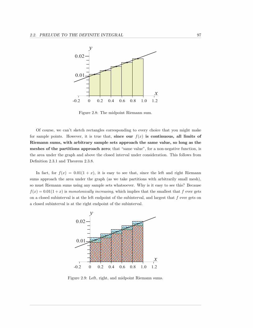
2.2. PRELUDE TO THE DEFINITE INTEGRAL 97
0.20-0.2 0.4 0.6 0.8 1.0 1.2x
y0.010.02
0.20-0.2 0.4 0.6 0.8 1.0 1.2x
y0.010.02
0.20-0.2 0.4 0.6 0.8 1.0 1.2x
y0.010.02
0.20-0.2 0.4 0.6 0.8 1.0 1.2x
y0.010.02
0.20-0.2 0.4 0.6 0.8 1.0 1.2x
y0.010.02
0.20-0.2 0.4 0.6 0.8 1.0 1.2x
y0.010.02
0.20-0.2 0.4 0.6 0.8 1.0 1.2x
y0.010.02
0.20-0.2 0.4 0.6 0.8 1.0 1.2x
y0.010.02Figure 2.8: The midpoint Riemann sum.
Of course, we can’t sketch rectangles corresponding to every choice that you might makefor sample points. However, it is true that, since our f(x) is continuous, all limits of
Riemann sums, with arbitrary sample sets approach the same value, so long as the
meshes of the partitions approach zero; that “same value”, for a non-negative function, isthe area under the graph and above the closed interval under consideration. This follows fromDefinition 2.3.1 and Theorem 2.3.8.
In fact, for f(x) = 0.01(1 + x), it is easy to see that, since the left and right Riemannsums approach the area under the graph (as we take partitions with arbitrarily small mesh),so must Riemann sums using any sample sets whatsoever. Why is it easy to see this? Becausef(x) = 0.01(1 + x) is monotonically increasing, which implies that the smallest that f ever getson a closed subinterval is at the left endpoint of the subinterval, and largest that f ever gets ona closed subinterval is at the right endpoint of the subinterval.
0.20-0.2 0.4 0.6 0.8 1.0 1.2x
y0.010.02
0.20-0.2 0.4 0.6 0.8 1.0 1.2x
y0.010.02
0.20-0.2 0.4 0.6 0.8 1.0 1.2x
y0.010.02
0.20-0.2 0.4 0.6 0.8 1.0 1.2x
y0.010.02
0.20-0.2 0.4 0.6 0.8 1.0 1.2x
y0.010.02
0.20-0.2 0.4 0.6 0.8 1.0 1.2x
y0.010.02
0.20-0.2 0.4 0.6 0.8 1.0 1.2x
y0.010.02
0.20-0.2 0.4 0.6 0.8 1.0 1.2x
y0.010.02
Figure 2.9: Left, right, and midpoint Riemann sums.
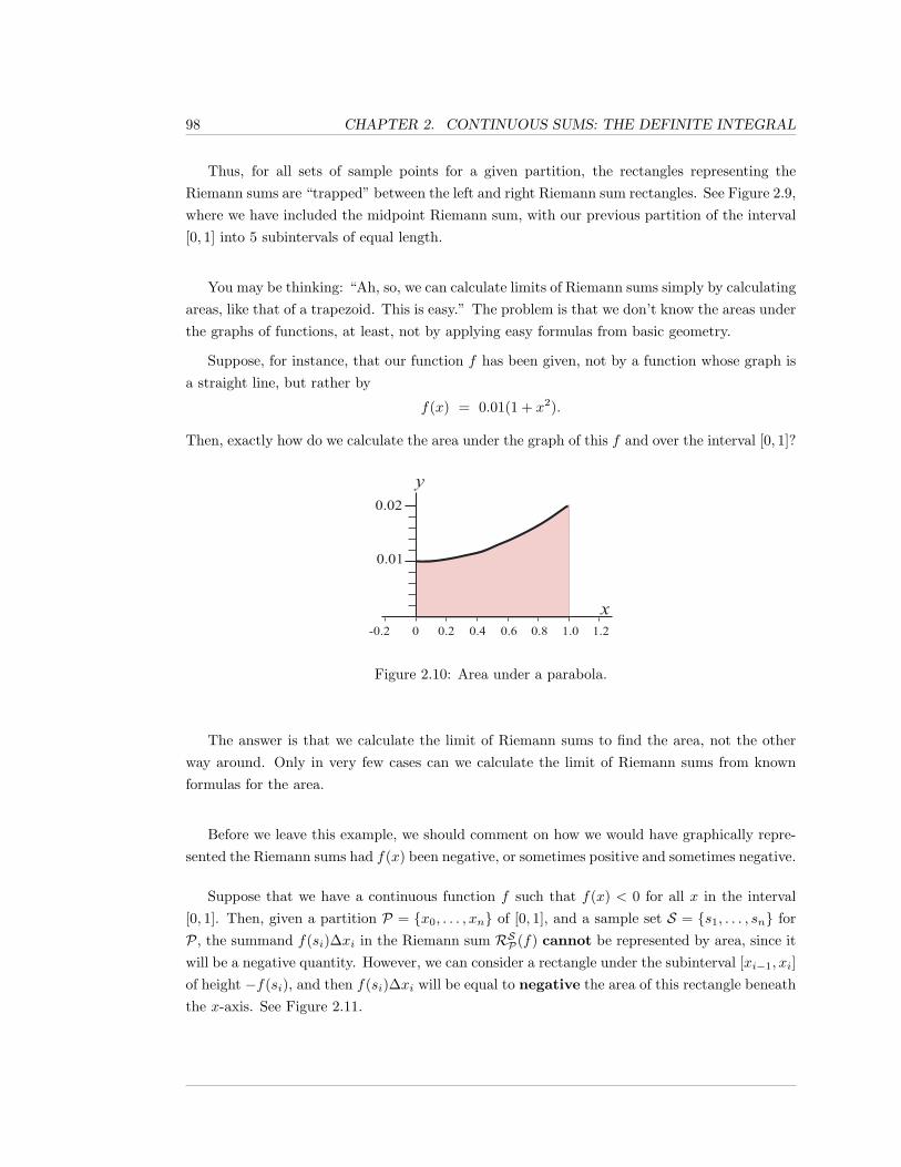
98 CHAPTER 2. CONTINUOUS SUMS: THE DEFINITE INTEGRAL
Thus, for all sets of sample points for a given partition, the rectangles representing theRiemann sums are “trapped” between the left and right Riemann sum rectangles. See Figure 2.9,where we have included the midpoint Riemann sum, with our previous partition of the interval[0, 1] into 5 subintervals of equal length.
You may be thinking: “Ah, so, we can calculate limits of Riemann sums simply by calculatingareas, like that of a trapezoid. This is easy.” The problem is that we don’t know the areas underthe graphs of functions, at least, not by applying easy formulas from basic geometry.
Suppose, for instance, that our function f has been given, not by a function whose graph isa straight line, but rather by
f(x) = 0.01(1 + x2).
Then, exactly how do we calculate the area under the graph of this f and over the interval [0, 1]?
0.20-0.2 0.4 0.6 0.8 1.0 1.2x
y0.010.02
Figure 2.10: Area under a parabola.
The answer is that we calculate the limit of Riemann sums to find the area, not the otherway around. Only in very few cases can we calculate the limit of Riemann sums from knownformulas for the area.
Before we leave this example, we should comment on how we would have graphically repre-sented the Riemann sums had f(x) been negative, or sometimes positive and sometimes negative.
Suppose that we have a continuous function f such that f(x) < 0 for all x in the interval[0, 1]. Then, given a partition P = {x0, . . . , xn} of [0, 1], and a sample set S = {s1, . . . , sn} forP, the summand f(si)∆xi in the Riemann sum RSP(f) cannot be represented by area, since itwill be a negative quantity. However, we can consider a rectangle under the subinterval [xi−1, xi]of height −f(si), and then f(si)∆xi will be equal to negative the area of this rectangle beneaththe x-axis. See Figure 2.11.
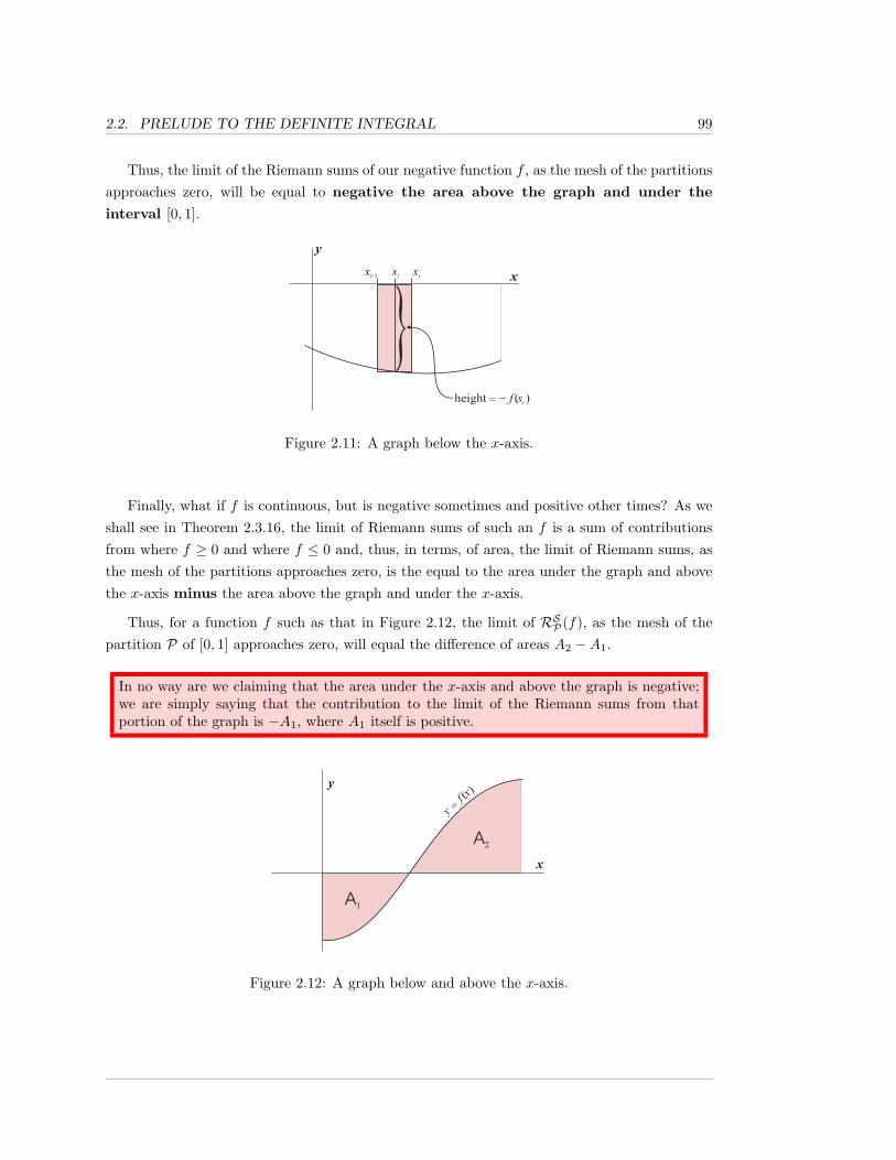
2.2. PRELUDE TO THE DEFINITE INTEGRAL 99
Thus, the limit of the Riemann sums of our negative function f , as the mesh of the partitionsapproaches zero, will be equal to negative the area above the graph and under the
interval [0, 1].
xi xy xi-1 si}_height f( )= si
xy )(f = y x
A1
A2
Figure 2.11: A graph below the x-axis.
Finally, what if f is continuous, but is negative sometimes and positive other times? As weshall see in Theorem 2.3.16, the limit of Riemann sums of such an f is a sum of contributionsfrom where f ≥ 0 and where f ≤ 0 and, thus, in terms, of area, the limit of Riemann sums, asthe mesh of the partitions approaches zero, is the equal to the area under the graph and abovethe x-axis minus the area above the graph and under the x-axis.
Thus, for a function f such as that in Figure 2.12, the limit of RSP(f), as the mesh of thepartition P of [0, 1] approaches zero, will equal the difference of areas A2 −A1.
In no way are we claiming that the area under the x-axis and above the graph is negative;we are simply saying that the contribution to the limit of the Riemann sums from thatportion of the graph is −A1, where A1 itself is positive.
xi xy xi-1 si}_height f( )= si
xy )(f = y x
A1
A2
Figure 2.12: A graph below and above the x-axis.
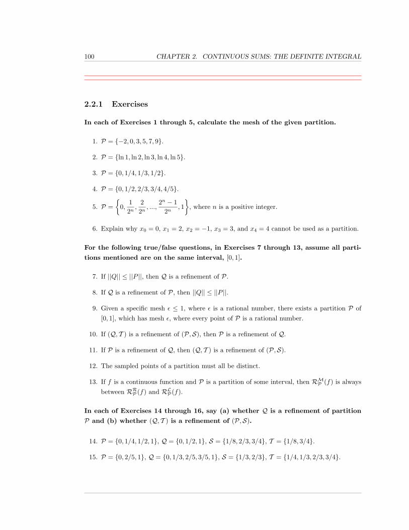
100 CHAPTER 2. CONTINUOUS SUMS: THE DEFINITE INTEGRAL
2.2.1 Exercises
In each of Exercises 1 through 5, calculate the mesh of the given partition.
1. P = {−2, 0, 3, 5, 7, 9}.
2. P = {ln 1, ln 2, ln 3, ln 4, ln 5}.
3. P = {0, 1/4, 1/3, 1/2}.
4. P = {0, 1/2, 2/3, 3/4, 4/5}.
5. P ={
0,12n,
22n, ...,
2n − 12n
, 1}
, where n is a positive integer.
6. Explain why x0 = 0, x1 = 2, x2 = −1, x3 = 3, and x4 = 4 cannot be used as a partition.
For the following true/false questions, in Exercises 7 through 13, assume all parti-
tions mentioned are on the same interval, [0, 1].
7. If ||Q|| ≤ ||P ||, then Q is a refinement of P.
8. If Q is a refinement of P, then ||Q|| ≤ ||P ||.
9. Given a specific mesh ε ≤ 1, where ε is a rational number, there exists a partition P of[0, 1], which has mesh ε, where every point of P is a rational number.
10. If (Q, T ) is a refinement of (P,S), then P is a refinement of Q.
11. If P is a refinement of Q, then (Q, T ) is a refinement of (P,S).
12. The sampled points of a partition must all be distinct.
13. If f is a continuous function and P is a partition of some interval, then RMP (f) is alwaysbetween RRP (f) and RLP(f).
In each of Exercises 14 through 16, say (a) whether Q is a refinement of partition
P and (b) whether (Q, T ) is a refinement of (P,S).
14. P = {0, 1/4, 1/2, 1}, Q = {0, 1/2, 1}, S = {1/8, 2/3, 3/4}, T = {1/8, 3/4}.
15. P = {0, 2/5, 1}, Q = {0, 1/3, 2/5, 3/5, 1}, S = {1/3, 2/3}, T = {1/4, 1/3, 2/3, 3/4}.
2.2. PRELUDE TO THE DEFINITE INTEGRAL 101
16. P = {0, 1/8, 2/5, 3/4, 1},Q = {0, 1/8, 3/13, 2/5, 5/9, 3/4, 4/5, 1}, S = {1/16, 2/5, 5/9, 3/4},T = {1/7, 4/21, 5/18, 1/2, 8/13, 7/9, 9/10}.
17. Suppose a car is traveling with variable velocity for three minutes, and that
• at some point between 0 and 40 seconds, the car is moving with velocity 15 m/s;
• at some point between 40 and 90 seconds, the car is moving with velocity 20 m/s;
• at some point between 90 and 120 seconds, the car is moving with velocity 25 m/s;
• at some point between 120 and 180 seconds, the car is moving with velocity 15 m/s.
Use Riemann sums to approximate the total displacement of the car from its initial posi-
tion.
18. Suppose a car is traveling with variable velocity for one hour, and that
• at some point between 0 and 12 minutes, the car is moving with velocity 40 miles/hour;
• at some point between 12 and 30 minutes, the car is moving with velocity -10miles/hour;
• at some point between 30 and 40 minutes, the car is moving with velocity 20 miles/hour;
• at some point between 40 and 60 minutes, the car is moving with velocity 0 miles/hour.
Use Riemann sums to approximate the total displacement of the car from its initial posi-tion.
19. Suppose a car is traveling with variable acceleration for 30 minutes, and that
• at some point between 0 and 10 minutes, the car is accelerating at a rate of 5 milesper hour per hour.
• at some point between 10 and 15 minutes, the car is accelerating at a rate of -3 milesper hour per hour.
• at some point between 15 and 25 minutes, the car is accelerating at a rate of 1 mileper hour per hour.
• at some point between 25 and 30 minutes, the car is accelerating at a rate of 4 milesper hour per hour.
Use Riemann sums to approximate the total change in velocity of the car from its initialvelocity.
20. Suppose that a balloon starts with no air in it, and is inflated between t = 0 and t = 90seconds. Suppose further that,
102 CHAPTER 2. CONTINUOUS SUMS: THE DEFINITE INTEGRAL
• at some time between 0 and 20 seconds, the balloon is inflating at a rate of 2 in3/s.
• at some time between 20 and 50 seconds, the balloon is inflating at a rate of 5 in3/s.
• at some time between 50 and 75 seconds, the balloon is inflating at a rate of -3 in3/s.Perhaps someone lost their grip on the balloon momentarily.
• at some time between 75 and 90 seconds, the balloon is inflating at a rate of 4 in3/s.
Use Riemann sums to approximate the total volume of air in the balloon at t = 90 seconds.
21. If f(t) = c on the interval [a, b], prove that the Riemann sum of f on [a, b] using anysample set and any partition is c(b− a). Give a physical interpretation of this fact if f is
a velocity function.
22. Let f(x) = mx be a line through the origin defined on [0, k]. Assume m > 0. What is thelimiting Riemann sum of this function over this interval? Use the fact that Riemann sumsapproximate the area under a curve. Your answer may be non-rigorous.
23. Suppose f is a continuous function on [a, b]. Then f achieves its minimum m and maximum
M . Let P be a partition of [a, b]. Prove that m(b− a) ≤ RP(f) ≤M(b− a).
24. Consider the following function with domain [0, 1].
f(x) =
{1, if x is rational;0, , if x is irrational.
Show that no matter what partition is chosen, and no matter how small its mesh, we canalways find two sets of sample point S = {si} and S ′ = {s′i} for that partition such thatthe Riemann sum is 1 on S and 0 on S ′.
In each of Exercises 25 through 27, calculate the left Riemann sum for the given
function and partition.
25. h(x) = −x, P = {−3,−2,−1, 0, 1, 2, 3}.
26. g(x) = sinx, P ={
0,π
4,π
2,
3π4, π
}.
27. f(x) = x2, P = {0, 0.1, 0.2, ..., 0.9, 1}.
In each of Exercises 28 through 30, calculate the right Riemann sum for the given
function and partition.
2.2. PRELUDE TO THE DEFINITE INTEGRAL 103
28. k(x) = ex/2, P = {0, ln 2, ln 3, ln 4}.
29. l(x) = e−x/2, P = {0, ln 2, ln 3, ln 4}.
30. j(x) = coshx, P = {0, ln 2, ln 3, ln 4}. Hint: Use the previous two problems and the factthat Riemann sums are linear, a fact you will prove in a later exercise.
In each of Exercises 31 through 34, calculate the midpoint Riemann sums for the
following functions and partitions.
31. y(x) = cosx, P = {− 3π2 ,−
π2 ,
π2 ,
3π2 }
32. r(x) = 1/x2, P = {1/10, 1/8, 1/5, 1/2, 1}.
33. g(x) = tan−1 x, P = {0, 1, 2, 3, 4}.
34. h(x) = sinx cosx, P = {0, π/2, π, 3π/2, 2π}.
35. Let f(x) =√
1− x2. Calculate the left Riemann sums for the following partitions.
a. P1 = {−1, 0, 1}.
b. P2 = {−1,−0.5, 0, 0.5, 1}.
c. P3 = {−1,−2/3,−1/3, 0, 1/3, 2/3, 1}.
d. Based on geometric intuition, what is the limiting Riemann sum, as the mesh ap-proaches 0, using partitions of the interval [−1, 1]?
36. Suppose f(x) is a continuous odd function. What is the midpoint Riemann sum using thepartition P = {−a3,−a2,−a1, 0, a1, a2, a3}, where 0 < a1 < a2 < a3?
The work done on an object experiencing a constant force F , as the object travels
along the x-axis, from point a to b, is W = F (b − a) (provided that the force acts
parallel to the x-axis).
The total work done on an object experiencing a variable force F = F (x) can
be approximated by Riemann sums. Namely, suppose P = {x0, x1, . . . , xn} is a par-
tition of [a, b] and that S = {s1, ..., sn} is a sample set for the partition. Then the
approximate work done is WSP(F ) =n∑i=1
F (si)(xi−xi−1). The metric units of work are
Newton-meters, or joules. C
In each of Exercises 37 through 39, assume an object moves along the interval
[0, 1], that the partition is P = {0, 1/4, 1/2, 3/4, 1}, and that the sample set is S ={1/4, 1/2, 3/4, 1}; calculate WSP(F ).
104 CHAPTER 2. CONTINUOUS SUMS: THE DEFINITE INTEGRAL
37. F (x) = x2.
38. F (x) = sin(πx).
39. F (x) = 3x.
40. Let f(x) = 1/x on the interval In = [ 1n , 1], where n = 2, 3, . . . . Let P =
{1n,
1n− 1
, , ...,12, 1}
.
Calculate the left Riemann sum of f over this partition using the left endpoints for n = 2, 3and 4.
41. Suppose that f and g are two continuous functions on the interval [a, b]. Let (P,S) bea partition and sample set for this interval. Prove that the Riemann sum is linear in thesense that
RSP(cf + g) = c · RSP(f) +RSP(g)
where c is any real number.
42. Consider the function,
h(x) =
{1x sin
(πx
), if 0 < x ≤ 1;
0, if x = 0,
and suppose that P is a partition of the interval [0, 1].
a. Show that the Riemann sums can be made arbitrarily large, i.e., for all N > 0, thereexists a sample set S such that RSP > N .
b. Similarly, show that the Riemann sums can be made arbitrarily small, i.e., for allN > 0, there exists a sample set S such that RSP < −N .
43. Consider the function
f(x) =
{3, if 0 ≤ x < 1 or 1 < x ≤ 2;100 x = 1.
a. Let Pn = {0, 12n ,
22n , ..., 2} be the uniform mesh where the distance between consecu-
tive points is 1/2n. Calculate RRPn(f),
b. Show that limn→∞
RRPn(f) = 6.
44. Let f(x) = c be a constant function on the interval [0, 1] with c > 0. Let
g(x) =
{c, if x 6= 1/2;0, if x = 1/2.
2.2. PRELUDE TO THE DEFINITE INTEGRAL 105
Let Pn be the partition on [0, 1] where the distance between each sample point is 1/n.Show that lim
n→∞RRP(f) = lim
n→∞RRP(g) = c.
The idea is that the Riemann sum of a function with a single discontinuity approaches theRiemann sum of the same function with the discontinuity removed.
Suppose that a partition P = {x0, x1, ..., xn} of the interval [a, b] has been given, and
that f is continuous on [a, b]. The Extreme Value Theorem tells us that f attains
maximum and minimum values on any closed subinterval of [a, b].
Let U(P) be a sample set chosen in such a way that, for each si in the sample
set U(P), f(si) equals the maximum value of f on [xi, xi+1]. Similarly, let L(P) be a
sample set chosen in such a way that, for each si in the sample set L(P), f(si) equals
the minimum value of f on [xi, xi+1].
45. Show that RU(P)P ≥ RL(P)
P .
46. Show that if Q is a refinement of P, then RU(Q)Q ≤ RU(P)
P and RL(Q)Q ≥ RL(P)
P .
47. Show that if P ′ is another partition, not necessarily a refinement of P or vice versa, thenRL(P)P ≤ RU(P′)
P′ .
We can use Riemann sums to approximate lengths as well as areas. Suppose we’d
like to approximate the length of the graph of a function f(x) on the interval [a, b].If P = {x0, x1, . . . , xn} is a partition of the interval [a, b], then we can measure the
lengths of the line segments connecting the points (xi−1, f(xi−1)), (xi, f(xi)). Recall
that this length is given by√
(xi − xi−1)2 + (f(xi)− f(xi−1))2.
48. Let f(x) =√
1− x2.
a. Consider the partition P1 = {−1, 0, 1} of [−1, 1]. Approximate the length of thegraph by calculating
2∑i=1
√(xi − xi−1)2 + (f(xi)− f(xi−1))2.
b. Approximate the length of the graph, via the same technique, but using the refinedpartition P2 = {−1,−1/2, 0, 1/2, 1}.
c. Based on classical geometry, what is the length of this graph? Are your approxima-tions close?
106 CHAPTER 2. CONTINUOUS SUMS: THE DEFINITE INTEGRAL
In each of Exercises 49 through 51, use the technique in the previous problem to
approximate the lengths of the graphs over the specified interval using the given
partition.
49. g(x) = sinx, [0, π], P = {0, π/4, π/2, 3π/4, π}.
50. h(x) = x2, [0, 1], P = {0, 1/4, 1/2, 3/4, 1}.
51. j(x) = 1/x, [1, 5], P = {1, 2, 3, 4, 5}.
52. Given a partition {x0, ..., xn} of [a, b], we’ve been using
n∑i=1
√(xi − xi−1)2 + (f(xi)− f(xi−1))2
to approximate the length of the graph of f on the interval [a, b]. This doesn’t look like aRiemann sum, but we can “fix” it.
Prove that, if f is differentiable on an open interval containing [a, b], and no two xi’s areequal, then there exists si in the open interval (xi−1, xi) such that
n∑i=1
√(xi − xi−1)2 + (f(xi)− f(xi−1))2 =
n∑i=1
(√1 + [f ′(si)]2
)∆xi.
2.3. THE DEFINITE INTEGRAL 107
2.3 The Definite Integral
As we saw in the previous section, the process of taking Riemann sums, and using partitionswith meshes that get arbitrarily small, arises in a number of different contexts. We might begiven the velocity of an object over an interval of time, and want to find the displacement. Wemight be given the rate at which a balloon is being inflated over an interval of time, and want toknow how much the volume of air in the balloon changes. We might be given a rod of variabledensity, and want to know its total mass. We might want to know how much area is “trapped”between the graph of a function and the x-axis.
In this section, we define the definite integral as the limit of Riemann sums, and discuss someof the basic properties of definite integrals. We do not give many applications of definite integralshere; such applications will be the sole topic of the entire next chapter, Chapter 3. It is alsosomewhat difficult to look at serious applications before we have the basic tool for calculatingdefinite integrals, the second part of the Fundamental Theorem of Calculus, Theorem 2.4.10.
Many of the proofs in this section are extremely technical and we have deferred them to theTechnical Matters section, Section 2.A.
In Example 2.2.8 and Example 2.2.9 in the previous section, we saw that our Riemann sums∑ni=1 f(si)∆xi approached a limit as we let the mesh of the partition approach zero, but we
used special partitions and sample sets; we used subintervals which all had the same length, andwe used the left and right Riemann sums. What we would like to know is that other manners ofchoosing partitions and sample sets would have approximated the same quantities, that is, wewould like to know that we could have used arbitrary partitions and arbitrary sample sets, andstill obtained the same limit, so long as the meshes of the partitions approach zero. Technically,this means that we would like for there to exist a limit L that our Riemann sums get arbitrarilyclose to (within ε, for arbitrary ε > 0) if we make the mesh of our partitions small enough (lessthan some δ > 0, where δ would typically depend on how ε was chosen).
Thus, we make the definition below, though it should not be clear at this point thatmany/any functions satisfy the strong requirements.
108 CHAPTER 2. CONTINUOUS SUMS: THE DEFINITE INTEGRAL
Definition 2.3.1. (The Definite Integral) Suppose that f is defined on the closed interval[a, b], where a < b, and that there exists a real number L such that, for all ε > 0, there existsδ > 0 such that, for all partitions P = {x0, . . . , xn} of [a, b], with mesh less than δ, and forall sample sets S = {s1, . . . , sn} for P,
∣∣∣∣∣n∑i=1
f(si)∆xi − L
∣∣∣∣∣ < ε.
Then, we write that
lim|| P ||→0
RSP(f) = lim|| P ||→0
n∑i=1
f(si)∆xi = L,
and we say that f is Riemann integrable on [a, b].
When f is Riemann integrable, the limit above is usually written
∫ b
a
f(x) dx,
and is called the (definite) integral of f on [a, b], or the integral of f(x), with respectto x, as x goes from a to b.
In this context, f is referred to as the integrand, and a and b are the limits of integration.
Remark 2.3.2. There are several points that we need to make now.
First, you should understand the point of the definition of the integral. A function is Riemannintegrable if and only if the Riemann sums
∑ni=1 f(si)∆xi approach a specific limit, regardless
of how you choose the partitions and/or sample points, as long as you take small enoughsubintervals in your partitions. You are allowed to use partitions in which the subintervals have
2.3. THE DEFINITE INTEGRAL 109
different lengths and choose sample points randomly. For f to be Riemann integrable meansthat none of this matters, as long as the mesh of the partitions approaches 0.
It’s the strongest property that you ask for, given our discussion in the previous section, andit’s a little difficult to believe that many interesting functions satisfy such a strong condition,but we shall see that most of the functions with which you’re familiar are, in fact, Riemannintegrable. (We are deliberately leaving you in suspense for the moment about which functionsthose are.)
We should also mention that it is customary in Calculus textbooks to drop the modifier“Riemann” from the term “Riemann integrable”, and simply say that a function is “integrable”,whenever they mean “Riemann integrable.” The justification given for this is always that“Riemann integrability is the only type of integrability that will be used in this textbook.”Strangely, this is not usually the case; every, or almost every, Calculus textbook includes adiscussion of improper integrals (see Section 2.5).
Improper integrals specifically involve defining an integral∫ baf(x) dx in certain cases where
f is not Riemann integrable on [a, b].
For this reason, we shall not drop the modifier “Riemann” from “Riemann integrable.” Weshall reserve the simpler term “integrable” for functions on intervals for which the Riemannintegral exists or for which the improper integral exists.
It is important to note that the units on the integral are the units of the Riemann sums, i.e.,the units of f times the units of x.
Finally, you should realize that the variable x, which appears in∫ b
a
f(x) dx, is a dummy
variable, which means that this variable name is irrelevant in the determining the actual valueof the integral. For instance, we have the following equalities:
∫ b
a
f(x) dx =∫ b
a
f(t) dt =∫ b
a
f(u) du.
All of these integrals mean the same thing: you partition the interval [a, b] into arbitrarily smallsubintervals, you evaluate f at a sample point in each subinterval, you multiply the values of fat the sample points times the lengths of the respective subintervals, you add, and you take thelimit of totals that you get, as the mesh of the partitions approaches zero. The point of writingall of that, without referring to a variable, was to make it clear that it is irrelevant what thevariable is.
However, it is true that, in applications, there will typically be variables of physical signifi-cance, like t for time or x for position, and it would, in fact, be a little odd to change the variable
110 CHAPTER 2. CONTINUOUS SUMS: THE DEFINITE INTEGRAL
name when writing integrals related to these quantities.
The fact that Definition 2.3.1 defines the Riemann integral as one single thing follows fromthe standard type of proof (see Theorem 2.A.1) that limits are unique; thus, there aren’t two(or more) different limits L1 and L2 that satisfy the ε-δ condition that we required. We statethis as a theorem.
Theorem 2.3.3. The limit of Riemann sums, the definite integral, given in Definition 2.3.1is unique, if it exists.
In addition, if f is Riemann integrable on the interval [a, b],∫ baf(x) dx = L, and
(Pn,Sn) is a sequence of sampled partitions of [a, b] such that limn→∞
|| Pn || = 0, then
limn→∞
RSnPn(f) = L.
Well, this is all great, but do we know any functions which are Riemann integrable?For that matter, do we know any functions which aren’t Riemann integrable? How you calculatedefinite integrals, when they exist, is a separate question, and our best answer to that will haveto wait until Section 2.4, but, for now, we’d at least like to know some results on when integralsexist and when they don’t.
There is an easy, fundamental, criterion which implies that a function is not Riemannintegrable. If a function is arbitrarily large in absolute value on an interval, then the functionwill not be Riemann integrable. We give a careful definition before stating this result as theorem.
Definition 2.3.4. A set E of real numbers is bounded if and only if there exist realnumbers p and q such that, for all x in E, p ≤ x ≤ q. Equivalently, E is bounded if andonly if there exists a real number M ≥ 0 such that, for all x in E, −M ≤ x ≤ M , i.e.,|x| ≤M .
Suppose that f is a real function and that a set E is contained in the domain of f . We saythat f is bounded on E if and only if the set of values of f on E is bounded, i.e., thereexists M ≥ 0 such that, for all x in E, |f(x)| ≤M .
If f is not bounded on E, then we say that f is unbounded on E.
2.3. THE DEFINITE INTEGRAL 111
Example 2.3.5. As a particular case of a bounded set, note that closed, bounded intervals areintervals of the form [a, b].
As an example of an unbounded function on a closed, bounded interval, consider
f(x) =
0 , if x = 0;1x, if 0 < x ≤ 1.
This function is unbounded on [0, 1], since f becomes arbitrarily large as x approaches 0 fromthe right.
On the other hand, the Extreme Value Theorem (see [2], or [4]) tells us that every contin-
uous function on a closed, bounded interval is bounded.
The most basic way in which a function can fail to be Riemann integrable is given by:
Theorem 2.3.6. If f is unbounded on the interval [a, b], then f is not Riemann integrableon [a, b].
Proof. Suppose that f is unbounded on [a, b], and let P = {x0, . . . , xn} be a partition of [a, b].Then, f must be unbounded on at least one of the subintervals [xi−1, xi]. Therefore, by changingthe sample point si in this subinterval, you can make |f(si)∆xi| arbitrarily large. This meansthat, as the mesh of the partitions approaches 0, the Riemann sums do not approach a limit thatis independent of how the sample points are chosen, i.e., the definite integral does not exist.
Example 2.3.7. Theorem 2.3.6 tells us immediately that the function f(x) from Example 2.3.5is not Riemann integrable.
112 CHAPTER 2. CONTINUOUS SUMS: THE DEFINITE INTEGRAL
Alright. Now we have a basic way in which functions can fail to be Riemann integrable. But,we want a theorem that tells us that lots of functions are Riemann integrable. There is such atheorem. Informally, what it says is that a function on a closed, bounded interval is Riemannintegrable if and only if the function is bounded and the set of points where the function isdiscontinuous is “small”. The technical requirement for “small” is that the set of points wheref is discontinuous has to have measure zero. A discussion of this result, in full generality, isbeyond the scope of the textbook. See [4] and [3].
However, all of the functions that we shall want to integrate in this book will either becontinuous, or have a finite number of discontinuities; the good news is that the empty set andfinite sets of points definitely have measure zero.
Thus, we have:
Theorem 2.3.8. Bounded functions on closed bounded intervals, which have, at most, afinite number of discontinuities, are Riemann integrable.
In particular, as continuous functions on closed, bounded intervals are bounded, all con-tinuous functions on closed, bounded intervals are Riemann integrable.
Proof. We give the proof in Theorem 2.A.5.
It is convenient to give a name to functions which may have, at most, a finite number ofdiscontinuities.
Definition 2.3.9. A real function f is piecewise-continuous on an interval I providedthat f is defined on I and is continuous at all, except (possibly) a finite number of, pointsin I. In particular, a continuous function is also piecewise-continuous.
Example 2.3.10. The function
g(x) =
0 , if 0 ≤ x ≤ 0.1;1x, if 0.1 < x ≤ 1
is piecewise-continuous and, hence, Theorem 2.3.8 tells that g(x) is Riemann integrable.
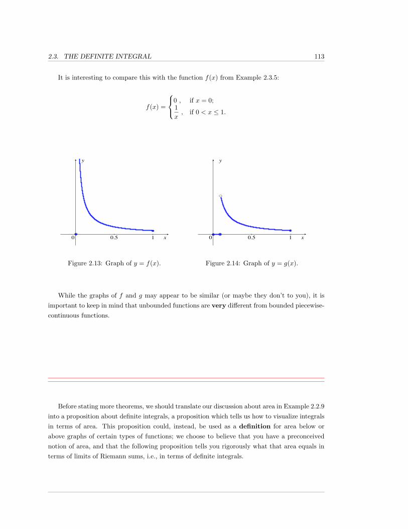
2.3. THE DEFINITE INTEGRAL 113
It is interesting to compare this with the function f(x) from Example 2.3.5:
f(x) =
0 , if x = 0;1x, if 0 < x ≤ 1.
0 0.5 1
Figure 2.13: Graph of y = f(x).
0 0.5 1
Figure 2.14: Graph of y = g(x).
While the graphs of f and g may appear to be similar (or maybe they don’t to you), it isimportant to keep in mind that unbounded functions are very different from bounded piecewise-continuous functions.
Before stating more theorems, we should translate our discussion about area in Example 2.2.9into a proposition about definite integrals, a proposition which tells us how to visualize integralsin terms of area. This proposition could, instead, be used as a definition for area below orabove graphs of certain types of functions; we choose to believe that you have a preconceivednotion of area, and that the following proposition tells you rigorously what that area equals interms of limits of Riemann sums, i.e., in terms of definite integrals.
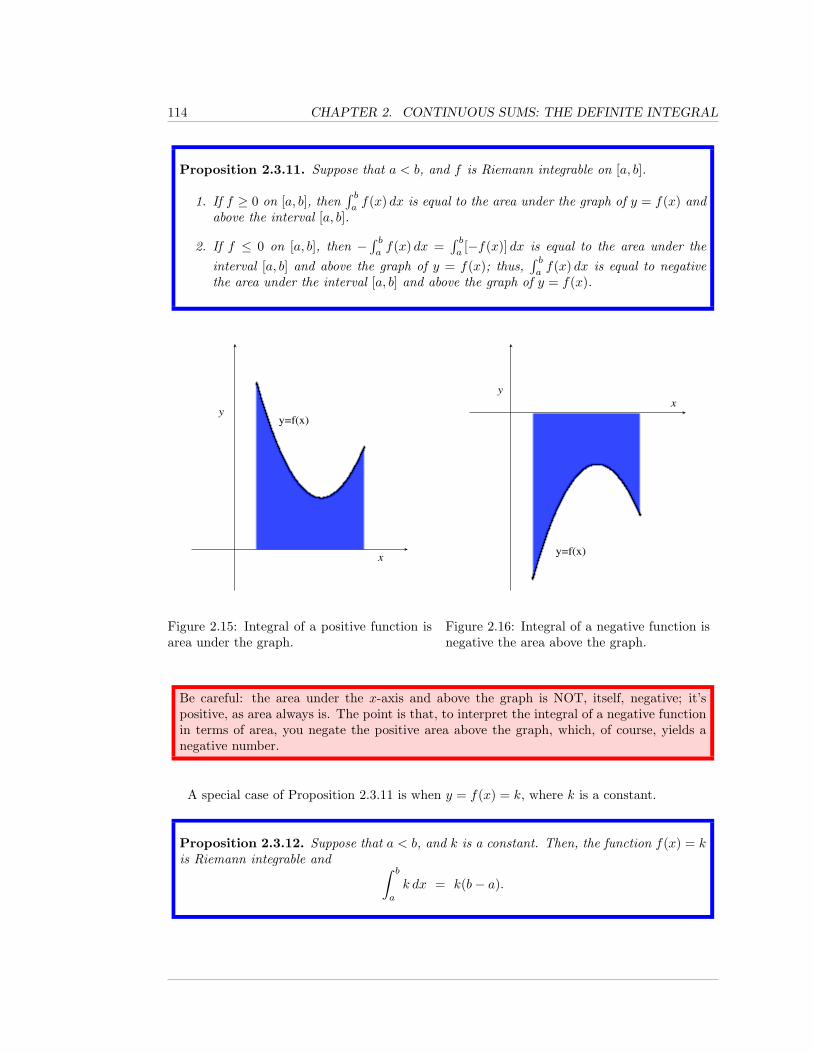
114 CHAPTER 2. CONTINUOUS SUMS: THE DEFINITE INTEGRAL
Proposition 2.3.11. Suppose that a < b, and f is Riemann integrable on [a, b].
1. If f ≥ 0 on [a, b], then∫ baf(x) dx is equal to the area under the graph of y = f(x) and
above the interval [a, b].
2. If f ≤ 0 on [a, b], then −∫ baf(x) dx =
∫ ba
[−f(x)] dx is equal to the area under theinterval [a, b] and above the graph of y = f(x); thus,
∫ baf(x) dx is equal to negative
the area under the interval [a, b] and above the graph of y = f(x).
y=f(x)
Figure 2.15: Integral of a positive function isarea under the graph.
y=f(x)
Figure 2.16: Integral of a negative function isnegative the area above the graph.
Be careful: the area under the x-axis and above the graph is NOT, itself, negative; it’spositive, as area always is. The point is that, to interpret the integral of a negative functionin terms of area, you negate the positive area above the graph, which, of course, yields anegative number.
A special case of Proposition 2.3.11 is when y = f(x) = k, where k is a constant.
Proposition 2.3.12. Suppose that a < b, and k is a constant. Then, the function f(x) = kis Riemann integrable and ∫ b
a
k dx = k(b− a).
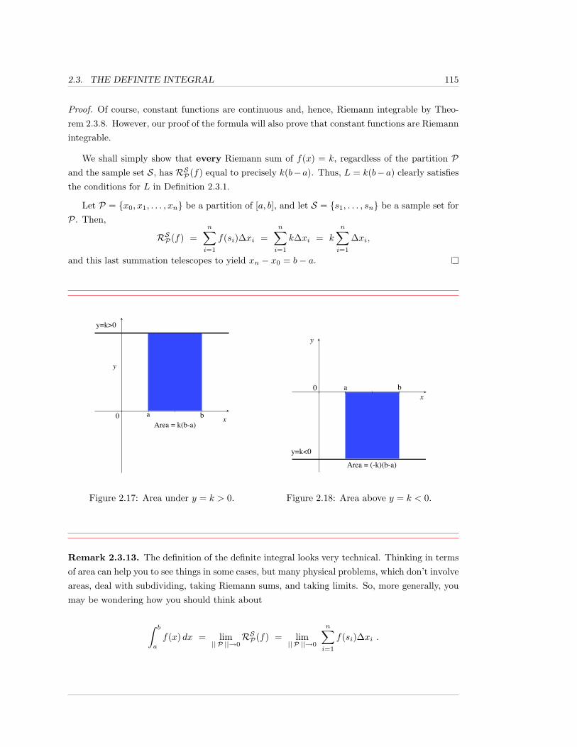
2.3. THE DEFINITE INTEGRAL 115
Proof. Of course, constant functions are continuous and, hence, Riemann integrable by Theo-rem 2.3.8. However, our proof of the formula will also prove that constant functions are Riemannintegrable.
We shall simply show that every Riemann sum of f(x) = k, regardless of the partition Pand the sample set S, has RSP(f) equal to precisely k(b−a). Thus, L = k(b−a) clearly satisfiesthe conditions for L in Definition 2.3.1.
Let P = {x0, x1, . . . , xn} be a partition of [a, b], and let S = {s1, . . . , sn} be a sample set forP. Then,
RSP(f) =n∑i=1
f(si)∆xi =n∑i=1
k∆xi = k
n∑i=1
∆xi,
and this last summation telescopes to yield xn − x0 = b− a.
y=k>0
a b0Area = k(b-a)
Figure 2.17: Area under y = k > 0.
y=k<0
a b0
Area = (-k)(b-a)
Figure 2.18: Area above y = k < 0.
Remark 2.3.13. The definition of the definite integral looks very technical. Thinking in termsof area can help you to see things in some cases, but many physical problems, which don’t involveareas, deal with subdividing, taking Riemann sums, and taking limits. So, more generally, youmay be wondering how you should think about
∫ b
a
f(x) dx = lim|| P ||→0
RSP(f) = lim|| P ||→0
n∑i=1
f(si)∆xi .
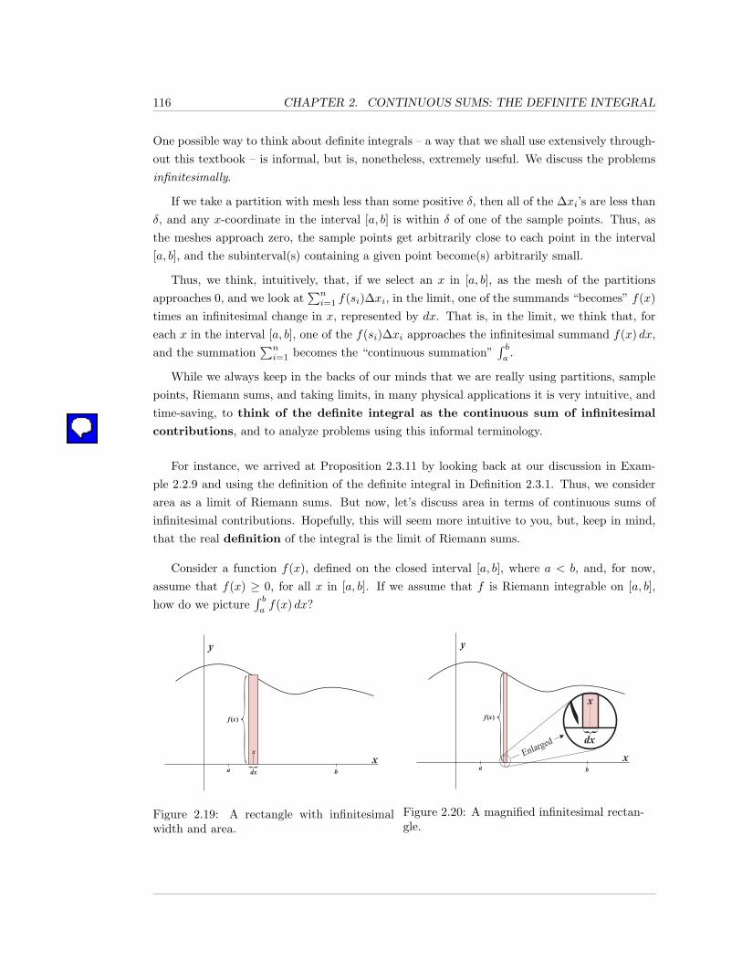
116 CHAPTER 2. CONTINUOUS SUMS: THE DEFINITE INTEGRAL
One possible way to think about definite integrals – a way that we shall use extensively through-out this textbook – is informal, but is, nonetheless, extremely useful. We discuss the problemsinfinitesimally.
If we take a partition with mesh less than some positive δ, then all of the ∆xi’s are less thanδ, and any x-coordinate in the interval [a, b] is within δ of one of the sample points. Thus, asthe meshes approach zero, the sample points get arbitrarily close to each point in the interval[a, b], and the subinterval(s) containing a given point become(s) arbitrarily small.
Thus, we think, intuitively, that, if we select an x in [a, b], as the mesh of the partitionsapproaches 0, and we look at
∑ni=1 f(si)∆xi, in the limit, one of the summands “becomes” f(x)
times an infinitesimal change in x, represented by dx. That is, in the limit, we think that, foreach x in the interval [a, b], one of the f(si)∆xi approaches the infinitesimal summand f(x) dx,and the summation
∑ni=1 becomes the “continuous summation”
∫ ba
.
While we always keep in the backs of our minds that we are really using partitions, samplepoints, Riemann sums, and taking limits, in many physical applications it is very intuitive, andtime-saving, to think of the definite integral as the continuous sum of infinitesimal
contributions, and to analyze problems using this informal terminology.
For instance, we arrived at Proposition 2.3.11 by looking back at our discussion in Exam-ple 2.2.9 and using the definition of the definite integral in Definition 2.3.1. Thus, we considerarea as a limit of Riemann sums. But now, let’s discuss area in terms of continuous sums ofinfinitesimal contributions. Hopefully, this will seem more intuitive to you, but, keep in mind,that the real definition of the integral is the limit of Riemann sums.
Consider a function f(x), defined on the closed interval [a, b], where a < b, and, for now,assume that f(x) ≥ 0, for all x in [a, b]. If we assume that f is Riemann integrable on [a, b],how do we picture
∫ baf(x) dx?
x
y
xdx
f ( )x
a b}
x
y
xdx
f ( )x
a b}
x
y
x dx
f ( )x
a b
Figure 2.19: A rectangle with infinitesimalwidth and area.
x
yf ( )x
a bxdx}
dxEnlarged
Figure 2.20: A magnified infinitesimal rectan-gle.
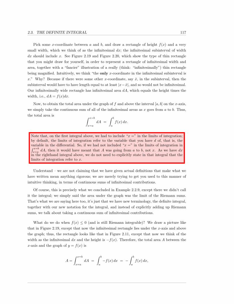
2.3. THE DEFINITE INTEGRAL 117
Pick some x-coordinate between a and b, and draw a rectangle of height f(x) and a verysmall width, which we think of as the infinitesimal dx; the infinitesimal subinterval of widthdx should include x. See Figure 2.19 and Figure 2.20, which show the type of thin rectanglethat you might draw for yourself, in order to represent a rectangle of infinitesimal width andarea, together with a “fancier” illustration of a really (think: “infinitesimally”) thin rectanglebeing magnified. Intuitively, we think “the only x-coordinate in the infinitesimal subinterval isx.” Why? Because if there were some other x-coordinate, say x, in the subinterval, then thesubinterval would have to have length equal to at least |x− x|, and so would not be infinitesimal.Our infinitesimally wide rectangle has infinitesimal area dA, which equals the height times thewidth, i.e., dA = f(x)dx.
Now, to obtain the total area under the graph of f and above the interval [a, b] on the x-axis,we simply take the continuous sum of all of the infinitesimal areas as x goes from a to b. Thus,the total area is ∫ x=b
x=a
dA =∫ b
a
f(x) dx.
Note that, on the first integral above, we had to include “x =” in the limits of integration;by default, the limits of integration refer to the variable that you have d of, that is, thevariable in the differential. So, if we had not included “x =” in the limits of integration in∫ x=b
x=adA, then it would have meant that A was going from a to b, not x. As we have dx
in the righthand integral above, we do not need to explicitly state in that integral that thelimits of integration refer to x.
Understand – we are not claiming that we have given actual definitions that make what wehave written mean anything rigorous; we are merely trying to get you used to this manner ofintuitive thinking, in terms of continuous sums of infinitesimal contributions.
Of course, this is precisely what we concluded in Example 2.2.9, except there we didn’t callit the integral; we simply said the area under the graph was the limit of the Riemann sums.That’s what we are saying here too, it’s just that we have new terminology, the definite integral,together with our new notation for the integral, and instead of explicitly adding up Riemannsums, we talk about taking a continuous sum of infinitesimal contributions.
What do we do when f(x) ≤ 0 (and is still Riemann integrable)? We draw a picture likethat in Figure 2.19, except that now the infinitesimal rectangle lies under the x-axis and abovethe graph; thus, the rectangle looks like that in Figure 2.11, except that now we think of thewidth as the infinitesimal dx and the height is −f(x). Therefore, the total area A between thex-axis and the graph of y = f(x) is
A =∫ x=b
x=a
dA =∫ b
a
−f(x) dx = −∫ b
a
f(x) dx,
118 CHAPTER 2. CONTINUOUS SUMS: THE DEFINITE INTEGRAL
and, hence,∫ baf(x) dx = −A. (Note that we “cheated” a bit here, and used that we could “pull
out” the negative sign in the integral; we won’t really know that this is “legal” until we haveTheorem 2.3.19.)
Finally, what do we do when f is Riemann integrable, and f(x) ≥ 0 on some (finite numberof) closed subintervals in [a, b], and f(x) ≤ 0 on (a finite number of) other closed subintervalsin [a, b]? In this case, as we discussed at the end of Example 2.2.9,
∫ baf(x) dx is a sum of
the contributions from where f ≥ 0 and where f ≤ 0, which means that∫ baf(x) dx can be
interpreted as the area under the graph of y = f(x) and above the interval [a, b] minus the areaabove the graph and under the interval [a, b]. (Again, we “cheated” a bit here, and used that wecould split the interval over [a, b] into the sum of integrals over subintervals whose union is [a, b];we won’t really know that this is “legal” until we have Theorem 2.3.16 and/or Theorem 2.3.18.)
We now need to state a number of theorem about definite integrals. Despite the fact thatall of the examples of Riemann integrable functions that we shall look at will be bounded,piecewise-continuous functions, the remaining theorems of this section are true for completelygeneral Riemann integrable functions, and it’s just as easy to state and prove them in thatgenerality; so we will.
The following theorem says that, as far as integration is concerned, you can “ignore” whathappens at a finite set of points in the domain. We give the proof in the Technical Matterssection; see Theorem 2.A.8.
Theorem 2.3.14. Suppose that f and g are defined on a closed interval [a, b], and that,except possibly for a finite set points in [a, b], f and g are equal at each point in [a, b].
Then, f is Riemann integrable on [a, b] if and only if g is, and when f and g are Riemannintegrable, ∫ b
a
f(x) dx =∫ b
a
g(x) dx.
Example 2.3.15. The function given by
f(x) =
{7 , if 1 ≤ x < 3 or 3 < x ≤ 5;4 , if x = 3
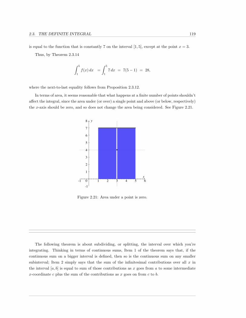
2.3. THE DEFINITE INTEGRAL 119
is equal to the function that is constantly 7 on the interval [1, 5], except at the point x = 3.
Thus, by Theorem 2.3.14
∫ 5
1
f(x) dx =∫ 5
1
7 dx = 7(5− 1) = 28,
where the next-to-last equality follows from Proposition 2.3.12.
In terms of area, it seems reasonable that what happens at a finite number of points shouldn’taffect the integral, since the area under (or over) a single point and above (or below, respectively)the x-axis should be zero, and so does not change the area being considered. See Figure 2.21.
-1 0 1 2 3 4 5 6-1
1
2
3
4
5
6
7
8
Figure 2.21: Area under a point is zero.
The following theorem is about subdividing, or splitting, the interval over which you’reintegrating. Thinking in terms of continuous sums, Item 1 of the theorem says that, if thecontinuous sum on a bigger interval is defined, then so is the continuous sum on any smallersubinterval; Item 2 simply says that the sum of the infinitesimal contributions over all x inthe interval [a, b] is equal to sum of those contributions as x goes from a to some intermediatex-coordinate c plus the sum of the contributions as x goes on from c to b.
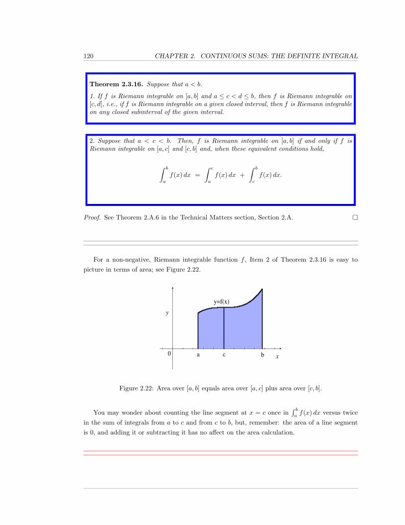
120 CHAPTER 2. CONTINUOUS SUMS: THE DEFINITE INTEGRAL
Theorem 2.3.16. Suppose that a < b.
1. If f is Riemann integrable on [a, b] and a ≤ c < d ≤ b, then f is Riemann integrable on[c, d], i.e., if f is Riemann integrable on a given closed interval, then f is Riemann integrableon any closed subinterval of the given interval.
2. Suppose that a < c < b. Then, f is Riemann integrable on [a, b] if and only if f isRiemann integrable on [a, c] and [c, b] and, when these equivalent conditions hold,
∫ b
a
f(x) dx =∫ c
a
f(x) dx +∫ b
c
f(x) dx.
Proof. See Theorem 2.A.6 in the Technical Matters section, Section 2.A.
For a non-negative, Riemann integrable function f , Item 2 of Theorem 2.3.16 is easy topicture in terms of area; see Figure 2.22.
a b0 c
y=f(x)
Figure 2.22: Area over [a, b] equals area over [a, c] plus area over [c, b].
You may wonder about counting the line segment at x = c once in∫ baf(x) dx versus twice
in the sum of integrals from a to c and from c to b, but, remember: the area of a line segmentis 0, and adding it or subtracting it has no affect on the area calculation.
2.3. THE DEFINITE INTEGRAL 121
The formula in Item 2 of Theorem 2.3.16 is so useful that we would like for it to be trueregardless of what inequalities (or equalities) are satisfied by a, b, and c. For instance, we wouldlike for the formula to hold if a = c. This means that we must have
∫ b
a
f(x) dx =∫ a
a
f(x) dx +∫ b
a
f(x) dx,
and so, we would need for∫ aaf(x) dx to equal 0.
Also, if a = b, we should have
∫ a
a
f(x) dx =∫ c
a
f(x) dx +∫ a
c
f(x) dx.
If∫ aaf(x) dx = 0, then we need for
∫ acf(x) dx to equal −
∫ caf(x) dx.
Therefore, we make the following definitions:
Definition 2.3.17. If a is in the domain of f , we say that f is Riemann integrable on theinterval [a, a] and define ∫ a
a
f(x) dx = 0.
If a < b, and f is Riemann integrable on [a, b], then we define
∫ a
b
f(x) dx = −∫ b
a
f(x) dx.
With the definitions above, and given Theorem 2.3.16, it is easy to check that
Theorem 2.3.18. Suppose that f is Riemann integrable on a closed interval containing a,b, and c, then ∫ b
a
f(x) dx =∫ c
a
f(x) dx +∫ b
c
f(x) dx,
regardless of the order of a, b, and c.
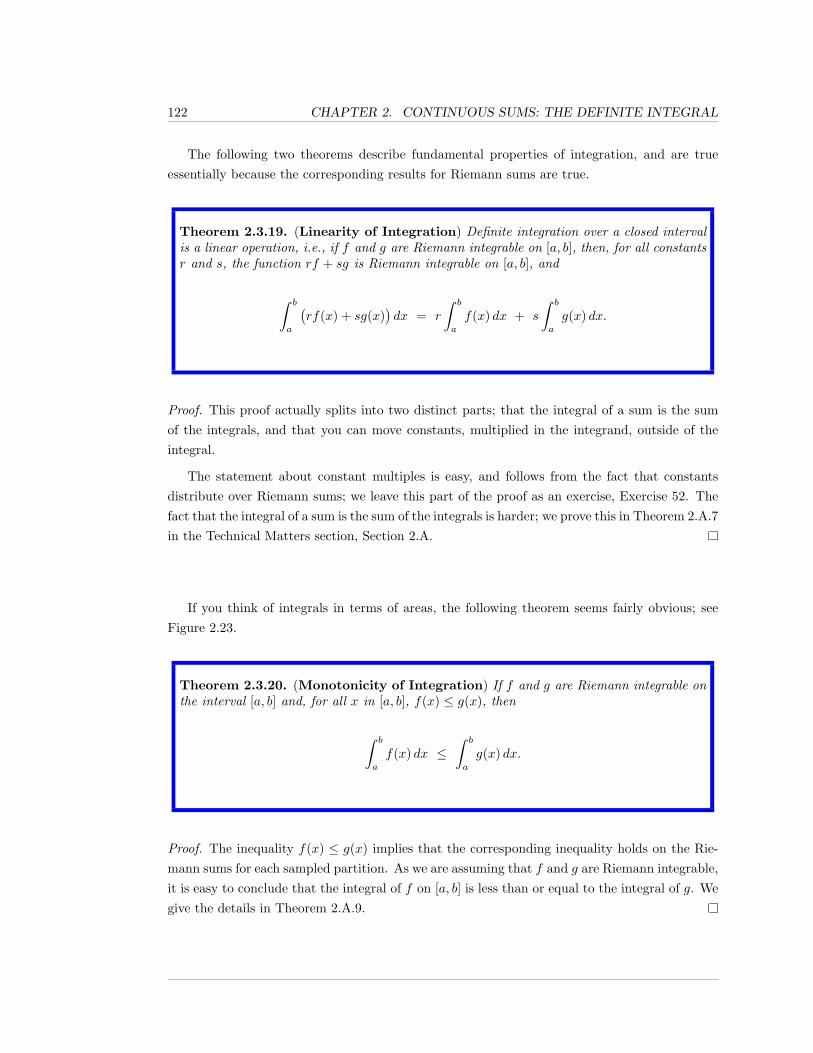
122 CHAPTER 2. CONTINUOUS SUMS: THE DEFINITE INTEGRAL
The following two theorems describe fundamental properties of integration, and are trueessentially because the corresponding results for Riemann sums are true.
Theorem 2.3.19. (Linearity of Integration) Definite integration over a closed intervalis a linear operation, i.e., if f and g are Riemann integrable on [a, b], then, for all constantsr and s, the function rf + sg is Riemann integrable on [a, b], and
∫ b
a
(rf(x) + sg(x)
)dx = r
∫ b
a
f(x) dx + s
∫ b
a
g(x) dx.
Proof. This proof actually splits into two distinct parts; that the integral of a sum is the sumof the integrals, and that you can move constants, multiplied in the integrand, outside of theintegral.
The statement about constant multiples is easy, and follows from the fact that constantsdistribute over Riemann sums; we leave this part of the proof as an exercise, Exercise 52. Thefact that the integral of a sum is the sum of the integrals is harder; we prove this in Theorem 2.A.7in the Technical Matters section, Section 2.A.
If you think of integrals in terms of areas, the following theorem seems fairly obvious; seeFigure 2.23.
Theorem 2.3.20. (Monotonicity of Integration) If f and g are Riemann integrable onthe interval [a, b] and, for all x in [a, b], f(x) ≤ g(x), then
∫ b
a
f(x) dx ≤∫ b
a
g(x) dx.
Proof. The inequality f(x) ≤ g(x) implies that the corresponding inequality holds on the Rie-mann sums for each sampled partition. As we are assuming that f and g are Riemann integrable,it is easy to conclude that the integral of f on [a, b] is less than or equal to the integral of g. Wegive the details in Theorem 2.A.9.

2.3. THE DEFINITE INTEGRAL 123
New A1 x
y
a bf ( )x
g ( )x
Figure 2.23: Comparing areas under the two graphs.
Theorem 2.3.21. If f is Riemann integrable on the interval [a, b], then so is |f |, and,
∣∣∣∣∣∫ b
a
f(x) dx
∣∣∣∣∣ ≤∫ b
a
|f(x)| dx.
Proof. The proof that f being Riemann integrable implies that |f | is Riemann integrable is verytechnical; we refer you to Theorem 3.3.5 of [4]. Assuming this fact, the given inequality followsas a corollary to Theorem 2.3.20 and Theorem 2.3.19.
To see this, note that −|f(x)| ≤ f(x) ≤ |f(x)|. Applying Theorem 2.3.20 and Theo-rem 2.3.19, we obtain that −|f | is Riemann integrable on [a, b] and
−∫ b
a
|f(x)| dx ≤∫ b
a
f(x) dx ≤∫ b
a
|f(x)| dx.
The inequality in the theorem is now immediate.
Now, consider the continuous function f(x) = x on a closed interval [a, b]. Theorem 2.3.8tells us that ∫ b
a
x dx
exists. Given that the integral exists, Theorem 2.3.3 tells us that we may calculate the valueof the integral by using the limit of Riemann sums over any sequence of sampled partitions, as
124 CHAPTER 2. CONTINUOUS SUMS: THE DEFINITE INTEGRAL
long as the meshes of the partitions approach zero.
So, we will let Pn be the partition of [a, b] into n subintervals of equal length, i.e., letting∆x = (b− a)/n,
Pn = {a, a+ ∆x, a+ 2∆x, . . . , a+ (n− 1)∆x, a+ n∆x},
where xi = a+ i∆x and, of course, b = a+ n∆x.
We will use the right Riemann sums, so that our sample points are also given by si = a+i∆x.Let’s denote the corresponding Riemann sum by simply Rn. For f(x) = x, we obtain
Rn =n∑i=1
f(si)∆xi =n∑i=1
[(a+ i∆x) ·∆x] .
Using linearity of summations, Proposition 2.1.4, and Item a from Corollary 2.1.11, we find
Rn = a∆xn∑i=1
1 + (∆x)2n∑i=1
i = an∆x + (∆x)2 · n(n+ 1)2
=
a(b− a) +(b− a)2
2· n
2 + n
n2= a(b− a) +
(b− a)2
2·(
1 +1n
).
Therefore, we find
∫ b
a
x dx = limn→∞
Rn = limn→∞
[a(b− a) +
(b− a)2
2·(
1 +1n
)]=
a(b− a) +(b− a)2
2= (b− a)
[a+
b− a2
]= (b− a) · b+ a
2=
b2 − a2
2.
Hence, we have shown
Proposition 2.3.22. ∫ b
a
x dx =b2
2− a2
2.
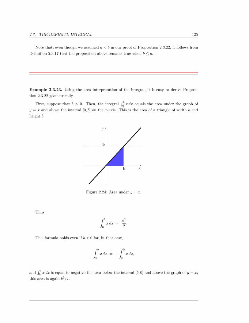
2.3. THE DEFINITE INTEGRAL 125
Note that, even though we assumed a < b in our proof of Proposition 2.3.22, it follows fromDefinition 2.3.17 that the proposition above remains true when b ≤ a.
Example 2.3.23. Using the area interpretation of the integral, it is easy to derive Proposi-tion 2.3.22 geometrically.
First, suppose that b > 0. Then, the integral∫ b
0x dx equals the area under the graph of
y = x and above the interval [0, b] on the x-axis. This is the area of a triangle of width b andheight b.
b
b
Figure 2.24: Area under y = x.
Thus, ∫ b
0
x dx =b2
2.
This formula holds even if b < 0 for, in that case,
∫ b
0
x dx = −∫ 0
b
x dx,
and∫ 0
bx dx is equal to negative the area below the interval [b, 0] and above the graph of y = x;
this area is again b2/2.
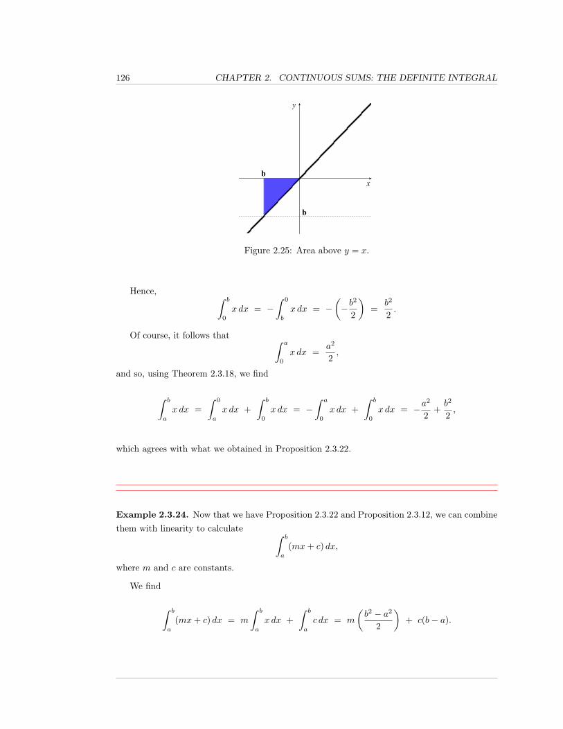
126 CHAPTER 2. CONTINUOUS SUMS: THE DEFINITE INTEGRAL
b
b
Figure 2.25: Area above y = x.
Hence, ∫ b
0
x dx = −∫ 0
b
x dx = −(−b
2
2
)=
b2
2.
Of course, it follows that ∫ a
0
x dx =a2
2,
and so, using Theorem 2.3.18, we find
∫ b
a
x dx =∫ 0
a
x dx +∫ b
0
x dx = −∫ a
0
x dx +∫ b
0
x dx = −a2
2+b2
2,
which agrees with what we obtained in Proposition 2.3.22.
Example 2.3.24. Now that we have Proposition 2.3.22 and Proposition 2.3.12, we can combinethem with linearity to calculate ∫ b
a
(mx+ c) dx,
where m and c are constants.
We find
∫ b
a
(mx+ c) dx = m
∫ b
a
x dx +∫ b
a
c dx = m
(b2 − a2
2
)+ c(b− a).
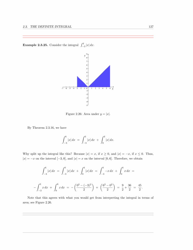
2.3. THE DEFINITE INTEGRAL 127
Example 2.3.25. Consider the integral∫ 6
−3|x| dx.
-7 -6 -5 -4 -3 -2 -1 0 1 2 3 4 5 6
-5
-4
-3
-2
-1
1
2
3
4
5
6
7
8
9
Figure 2.26: Area under y = |x|.
By Theorem 2.3.16, we have
∫ 6
−3
|x| dx =∫ 0
−3
|x| dx +∫ 6
0
|x| dx.
Why split up the integral like this? Because |x| = x, if x ≥ 0, and |x| = −x, if x ≤ 0. Thus,|x| = −x on the interval [−3, 0], and |x| = x on the interval [0, 6]. Therefore, we obtain
∫ 6
−3
|x| dx =∫ 0
−3
|x| dx +∫ 6
0
|x| dx =∫ 0
−3
−x dx +∫ 6
0
x dx =
−∫ 0
−3
x dx +∫ 6
0
x dx = −(
02 − (−3)2
2
)+(
62 − 02
2
)=
92
+362
=452.
Note that this agrees with what you would get from interpreting the integral in terms ofarea; see Figure 2.26.
128 CHAPTER 2. CONTINUOUS SUMS: THE DEFINITE INTEGRAL
Example 2.3.26. The cosine function is continuous and, for all x, −1 ≤ cosx ≤ 1. If we wantbounds on the integral of cosx, we can apply Theorem 2.3.20 twice.
For instance, even though we do not yet know how to calculate∫ π/2
0cosx dx, we can conclude
that
−π2
=∫ π/2
0
−1 dx ≤∫ π/2
0
cosx dx ≤∫ π/2
0
1 dx =π
2.
In fact, as we shall see later,∫ π/2
0cosx dx = 1, which is, indeed, between −π/2 and π/2.
Proposition 2.3.27. ∫ b
a
x2 dx =b3
3− a3
3.
Proof. We will prove that, if b > 0, then∫ b
0x2 dx = b3/3. The case where b < 0 is similar, and
we leave it as an exercise. Once you know that∫ b
0x2 dx = b3/3, the proposition follows from
applying Theorem 2.3.18:
∫ b
a
x2 dx =∫ 0
a
x2 dx +∫ b
0
x2 dx = −∫ a
0
x2 dx +∫ b
0
x2 dx =
−a3
3+b3
3.
So, assume that b > 0. How do we show that∫ b
0x2 dx = b3/3? As x2 is continuous, we know
that the integral exists, and so we may calculate it by taking a limit of Riemann sums, in whichthe meshes of our partitions approach 0. This was how we derived Proposition 2.3.22.
Let Pn be the partition of [0, b] into n subintervals of equal length, i.e., the partition in whichxi = ib/n, and ∆xi = b/n. If we once again use right Riemann sums, our sample set Rn is theone in which si also equals ib/n.
Our corresponding Riemann sum for x2 is
Rn =n∑i=1
(ib
n
)2
· bn
=b3
n3
n∑i=1
i2.
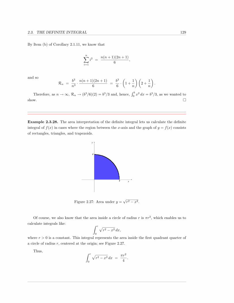
2.3. THE DEFINITE INTEGRAL 129
By Item (b) of Corollary 2.1.11, we know that
n∑i=1
i2 =n(n+ 1)(2n+ 1)
6,
and soRn =
b3
n3· n(n+ 1)(2n+ 1)
6=
b3
6·(
1 +1n
)(2 +
1n
).
Therefore, as n→∞, Rn → (b3/6)(2) = b3/3 and, hence,∫ b
0x2 dx = b3/3, as we wanted to
show.
Example 2.3.28. The area interpretation of the definite integral lets us calculate the definiteintegral of f(x) in cases where the region between the x-axis and the graph of y = f(x) consistsof rectangles, triangles, and trapezoids.
r
r
Figure 2.27: Area under y =√r2 − x2.
Of course, we also know that the area inside a circle of radius r is πr2, which enables us tocalculate integrals like: ∫ r
0
√r2 − x2 dx,
where r > 0 is a constant. This integral represents the area inside the first quadrant quarter ofa circle of radius r, centered at the origin; see Figure 2.27.
Thus, ∫ r
0
√r2 − x2 dx =
πr2
4.
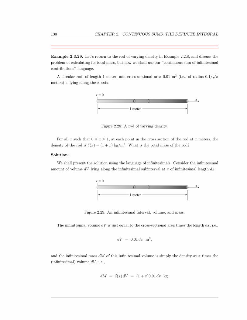
130 CHAPTER 2. CONTINUOUS SUMS: THE DEFINITE INTEGRAL
Example 2.3.29. Let’s return to the rod of varying density in Example 2.2.8, and discuss theproblem of calculating its total mass, but now we shall use our “continuous sum of infinitesimalcontributions” language.
A circular rod, of length 1 meter, and cross-sectional area 0.01 m2 (i.e., of radius 0.1/√π
meters) is lying along the x-axis.
Figure 2.28: A rod of varying density.
For all x such that 0 ≤ x ≤ 1, at each point in the cross section of the rod at x meters, thedensity of the rod is δ(x) = (1 + x) kg/m3. What is the total mass of the rod?
Solution:
We shall present the solution using the language of infinitesimals. Consider the infinitesimalamount of volume dV lying along the infinitesimal subinterval at x of infinitesimal length dx.
Figure 2.29: An infinitesimal interval, volume, and mass.
The infinitesimal volume dV is just equal to the cross-sectional area times the length dx, i.e.,
dV = 0.01 dx m3,
and the infinitesimal mass dM of this infinitesimal volume is simply the density at x times the(infinitesimal) volume dV , i.e.,
dM = δ(x) dV = (1 + x)0.01 dx kg.
2.3. THE DEFINITE INTEGRAL 131
Finally, the total mass M of the rod is the continuous sum of all of the infinitesimal masses asx goes from 0 to 1 meter, i.e.,
M =∫ x=1
x=0
dM =∫ 1
0
(1 + x)0.01 dx kg.
Suppose that a < b. We now want to develop a reasonable notion of “the mean, or average,value of f on the interval [a, b].”
What should the average value of f mean? Well...if there were a finite number of f -values,we would simply add up all of the values and then divided by the number of values; this is whatis normally meant by the “average” or “mean”. The problem, of course, is that we have aninfinite number of values f(x), one for each x in the interval [a, b]. How do we deal with this?
As you may have guessed, we take the average of a finite number of f -values, and then takea limit. Let n ≥ 1 be an integer. Subdivide the interval [a, b] into n subintervals of equal length∆x = (b− a)/n. As usual, in the i-th subinterval, we pick a sample point si. We may now takethe average value of f at the n sample points; we obtain
f(s1) + f(s2) + · · ·+ f(sn)n
=
n∑i=1
f(si)
n.
So, what would be a reasonable notion of the average value of f on the entire interval? Wecan try taking the limit of the average above, as n approaches ∞, but why would this limitexist, and what does it have to do with integration?
Things become more clear if we multiply the numerator and denominator of the abovefractions by ∆x. Then, we obtain
n∑i=1
f(si)∆x
n∆x=
n∑i=1
f(si)∆x
b− a.
If f is Riemann integrable on [a, b], then, as n→∞, this last numerator approaches∫ baf(x) dx,
132 CHAPTER 2. CONTINUOUS SUMS: THE DEFINITE INTEGRAL
and so, the limit of the average value of f at the sample points approaches
1b− a
∫ b
a
f(x) dx.
Therefore, we make the following definition:
Definition 2.3.30. Suppose that a < b and that f is Riemann integrable on [a, b]. Then,we define the mean value, or average value, of f on [a, b] to be
1b− a
∫ b
a
f(x) dx.
For continuous functions, we have the following theorem about the mean value of f .
Theorem 2.3.31. (Mean Value Theorem for Integration) Suppose that f is continu-ous on the closed interval [a, b]. Then, there exists c in [a, b] such that
∫ b
a
f(x) dx = (b− a)f(c).
Thus, if a < b, there exists c in the interval [a, b] such that f(c) equals the mean valueof f on [a, b], i.e., f attains its mean value on [a, b] at some point in [a, b].
Proof. If a = b, then the theorem is obviously true. So, assume that a < b.
As f is continuous on [a, b], the Extreme Value Theorem (see [2]), tells us that f attains aglobal minimum value m on [a, b] and a global maximum value M on [a, b].
Thus, for all x in [a, b], m ≤ f(x) ≤M . By Theorem 2.3.20, this implies that
m(b− a) =∫ b
a
mdx ≤∫ b
a
f(x) dx ≤∫ b
a
M dx = M(b− a).
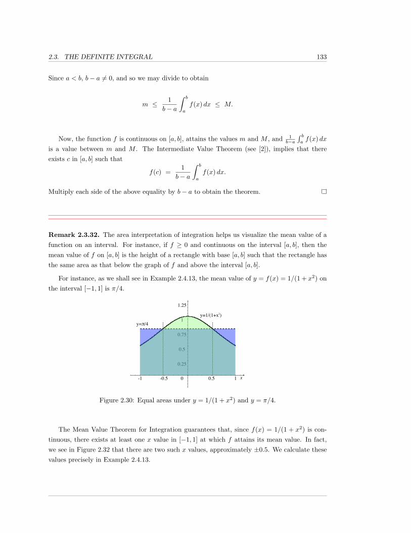
2.3. THE DEFINITE INTEGRAL 133
Since a < b, b− a 6= 0, and so we may divide to obtain
m ≤ 1b− a
∫ b
a
f(x) dx ≤ M.
Now, the function f is continuous on [a, b], attains the values m and M , and 1b−a
∫ baf(x) dx
is a value between m and M . The Intermediate Value Theorem (see [2]), implies that thereexists c in [a, b] such that
f(c) =1
b− a
∫ b
a
f(x) dx.
Multiply each side of the above equality by b− a to obtain the theorem.
Remark 2.3.32. The area interpretation of integration helps us visualize the mean value of afunction on an interval. For instance, if f ≥ 0 and continuous on the interval [a, b], then themean value of f on [a, b] is the height of a rectangle with base [a, b] such that the rectangle hasthe same area as that below the graph of f and above the interval [a, b].
For instance, as we shall see in Example 2.4.13, the mean value of y = f(x) = 1/(1 + x2) onthe interval [−1, 1] is π/4.
-1 -0.5 0 0.5 1
-0.25
0.25
0.5
0.75
1
1.25
1.5
y=!/4
y=1/(1+x )2
y=1/(1+x )2
Figure 2.30: Equal areas under y = 1/(1 + x2) and y = π/4.
The Mean Value Theorem for Integration guarantees that, since f(x) = 1/(1 + x2) is con-tinuous, there exists at least one x value in [−1, 1] at which f attains its mean value. In fact,we see in Figure 2.32 that there are two such x values, approximately ±0.5. We calculate thesevalues precisely in Example 2.4.13.
134 CHAPTER 2. CONTINUOUS SUMS: THE DEFINITE INTEGRAL
2.3.1 Exercises
Calculate the definite integrals.
1.∫ 7
3
5 dx.
2.∫ 6
−3
5t− 7 dt.
3.∫ 8
−4
|u− 4|+ 2 du.
4.∫ 7
−3
2|4− 8z| dz.
5.∫ 12
0
5w2 dw.
6.∫ 7
−3
(v + 3) dv.
7.∫ −3
2
x2 + x dx.
8.∫ 6
−4
f(x) dx, where f(x) =
{3 x < −1−5 x ≥ −1.
9.∫ 4
4
e−x2dx.
Answer the following true/false questions. If the statement is true, why is it true?
If the statement is false, provide a counterexample.
10. If f is differentiable on an open interval containing [a, b], then∫ b
a
f(x) dx exists.
11. If∫ b
a
f(x) dx ≤∫ b
a
g(x) dx, then f(x) ≤ g(x) for all x ∈ [a, b].
12. If f is integrable, then f is continuous.
13.∫ b
a
f(x) dx =∫ a
b
f(x) dx for all integrable functions f .
2.3. THE DEFINITE INTEGRAL 135
In each of exercises 14 through 18, calculate the average value of the function over
the interval.
14. c(x) = −10, [−11, 9].
15. g(x) = 12x− 10, [4, 9].
16. h(x) =x2
6, [0, 12].
17. m(t) = |t|+ 3, [−3, 6].
18. p(x) =
{2x x 6= 10 x = 1
, [−2, 4].
19. Recall that the height of a projectile with initial velocity v0 and h0 is
h(t) = −12gt2 + v0t+ h0.
Calculate the average height between times t = 0 and t = t1.
20. Prove that the function f(x) =
{0, if x is rational;1, if x is irrational
is not integrable.
21. Construct an example of a function that is integrable but that does not satisfy the meanvalue property. That is, construct a function that does not achieve its average value overits domain.
In each of Exercises 22 through 25, you are given the velocity function of a parti-
cle, in meters per second. Calculate the average velocity of the function over the
specified interval.
22. v(t) = 3t+ 2, [4, 8].
23. v(t) = t2 − 5t+ 3, [2, 6].
24. v(t) = t3 − 2t2 + 3t+ 2, [−1, 3].
25. v(t) = |t− 4|, [2, 6].
In Exercises 26 - 29, you are given the same velocity function and interval as in the
previous four problems. For each problem, calculate (a) the acceleration function,
and (b) the average acceleration over the interval.
136 CHAPTER 2. CONTINUOUS SUMS: THE DEFINITE INTEGRAL
26. v(t) = 3t+ 2, [4, 8].
27. v(t) = t2 − 5t+ 3, [2, 6].
28. v(t) = t3 − 2t2 + 3t+ 2, [−1, 3].
29. v(t) = |t− 4|, [2, 6].
30. Suppose p1(t) and p2(t) are the position functions of two particles and that p2(t) = p1(t)+Cwhere C is some constant. The position functions have common domain [a, b].
a. What is the relationship between the average positions of the two particles?
b. What is the relationship between the average velocities of the two particles?
c. What is the relationship between the average accelerations of the two particles?
31. Suppose that v1(t) and v2(t) are the velocity functions of two particles and that v2(t) =v1(t) + C where C is some constant. The velocity functions have common domain [a, b].
a. What is the relationship between the average velocities of the two particles?
b. What is the relationship between the average accelerations of the two particles?
32. Is the function below integrable on [−π, π]?
f(x) =
{sin(1/x) x 6= 00 x = 0.
33. Is the function below integrable on [−π, π]?
g(x) =
{x sin(1/x) x 6= 00 x = 0.
Estimate the definite integrals using the given partitions using the left endpoint
sample set.
34.∫ 1
0
sin(πx) dx, P = {0, 1/4, 1/2, 3/4, 1}.
35.∫ 1
0
√x dx, P = {0, 1/4, 1/3, 3/4, 1}.
36.∫ 1
−1
11 + x2
dx, P = {−1,−1/2, 0, 1/2, 1}.
2.3. THE DEFINITE INTEGRAL 137
37.∫ 1
−1
coshx dx, P = {−1,−1/2, 0, 1/2, 1}.
Calculate the definite integrals below by determining the area enclosed between
their graphs and the x-axis. Remember that area below the x-axis is counted with
a minus sign in the integral.
38.∫ 7
−4
2x− 3 dx.
39.∫ 5
−5
√25− x2 + 4 dx.
40.∫ 6
2
|x− 3|+ 5 dx.
The idea of using integrals to calculate the area between a curve and the x-axis can
be generalized. To calculate the area of the region between the graphs of f(x) and
g(x), we just need to notice that if f > g ≥ 0, then the area between the graphs
of f and g is the area bounded by the graph of f and the x-axis minus the area
bounded by the graph of g and the x-axis. By the linearity of the integral, this area
is given by∫ b
a
(f(x)−g(x)
)dx. In each of Exercises 41 through 44, calculate the area
bounded by the two graphs along the interval.
41. f(x) = 4x, g(x) = 2, [8, 12].
42. f(x) = 5x, g(x) = 3x, [0, 10].
43. f(x) = x, g(x) = x2, [0, 1].
44. f(x) =√
25− x2, g(x) = 3, [−4, 4].
45. Consider a triangle contained entirely in the first quadrant with vertices P = (x1, y1),Q = (x2, y2) and R = (x2, y3). Assume further that x1 < x2 and that y3 > y2.
a. Show that the equations of the lines between P and R, and P and Q are
f(x) =y3 − y1
x2 − x1x− x2(y3 − y1)
x2 − x1+ y3
g(x) =y2 − y1
x2 − x1x− x2(y2 − y1)
x2 − x1+ y2
respectively.
138 CHAPTER 2. CONTINUOUS SUMS: THE DEFINITE INTEGRAL
b. Calculate∫ x2
x1
f(x)− g(x) dx and conclude that the area of the triangle is
12
[x2y3 − x2y2 + x1y2 − x1y3] =12
(x1 − x2)(y2 − y3).
46. Suppose a 10 meter long rod lies along the x-axis The rod is a rectangular prism withcross-sectional area 2 m2. The density of the rod is given by δx = (x2 + 1) kg / m3.Express the total mass of the rod in terms of a definite integral. You need not calculatethe integral.
47. Suppose a 10 meter metallic cone lies along the x-axis with its vertex at the origin. Morespecifically, the projection of the cone onto the xy plane is defined by the line segmentsy = x and y = −x for x ∈ [0, 10]. The density at each point in the cross section of the rodis given by δ(x) = (12−x) kg/m3. Express the total mass of the cone in terms of a definiteintegral. You need not calculate the integral. Hint: in this case, dA, the infinitesimal area,is no longer constant.
Recall that a parameterized planar curve with domain [a, b] is a map ~α(t) into the
xy-plane. That is, ~α(t) = (x(t), y(t)). Definite integrals can be used to calculate the
length of curves. Specifically, if ~α(t) is a differentiable curve on [a, b], the length of
the curve is∫ b
a
|~α′(t)| dt. Calculate the lengths of the curves in Exercises 48 - 51.
48. ~α(t) = (t, 3), [−2, 4].
49. ~α(t) = (t, 4t), [0, 5].
50. ~α(t) = (t,mt), [a, b].
51. ~α(t) = (R cos t, R sin t), [0, π], where R ≥ 0.
52. Prove the constant multiple portion of Theorem 2.3.19, i.e., prove that if f is Riemannintegrable on the closed interval [a, b] and c is a constant, then cf is Riemann integrableon [a, b], and ∫ b
a
cf(x) dx = c
∫ b
a
f(x) dx.
2.4. THE FUNDAMENTAL THEOREM OF CALCULUS 139
2.4 The Fundamental Theorem of Calculus
The definite integral has many applications, all of which stem from the fact that the definition ofthe definite integral as a limit of Riemann sums makes the definite integral a “continuous sum ofinfinitesimal contributions”. However, actually calculating definite integrals by taking limits ofRiemann sums is extraordinarily painful, and, for definite integrals to really be manageable, weneed an easy way to calculate these limits of Riemann sums that come up in so many physicalsituations.
The second part of the Fundamental Theorem of Calculus, Theorem 2.4.10, provides this“easy” method; it tells us that we may calculate definite integrals by anti-differentiating. Thistheorem is truly “fundamental”, for it tells us that the two basics ideas of Calculus, differentiatingand integrating, are inextricably related.
In Proposition 2.3.12, Proposition 2.3.22, and Proposition 2.3.27, we gave formulas for thedefinite integrals of f(x) = k, g(x) = x, and h(x) = x2 over the interval [a, b]. Those formulasmay not have had an obvious pattern, but it may become clear what’s going on after we introducesome new notation.
Definition 2.4.1. If F (x) is a real function, defined at x = a and x = b, then we definethe evaluation notation,
∣∣ba
by
F (x)∣∣ba
= F (b)− F (a).
We also writeF (x)
∣∣x=b
x=a= F (b)− F (a),
if we want to emphasize the name of the variable that takes on the values a and b.
We read this as: F evaluated from a to b, or F (x) evaluated from x = a to x = b.
Now that we have this new notation, let’s rewrite our formulas from Proposition 2.3.12,Proposition 2.3.22, and Proposition 2.3.27. We have
∫ b
a
k dx = k(b− a) = kx∣∣ba,
140 CHAPTER 2. CONTINUOUS SUMS: THE DEFINITE INTEGRAL
∫ b
a
x dx =b2
2− a2
2=
x2
2
∣∣∣ba,
and
∫ b
a
x2 dx =b3
3− a3
3=
x3
3
∣∣∣ba.
Do you see the pattern here? It may not be clear from just three examples, but you may beable to guess what happens more generally.
In each of the three formulas above, the derivative of the function being evaluated from a tob on the right is precisely the function being integrated from a to b on the left. In other words,the function being evaluated from a to b on the right is an anti-derivative of the integrand.
Is this true more generally? YES. This result is part of the Fundamental Theorem ofCalculus, and it is the reason that the notation
∫f(x) dx and terminology “indefinite integral”
for anti-derivatives are so similar to the notation and terminology for definite integrals.
Once we have the Fundamental Theorem, we will no longer need to compute definite integralsby the cumbersome process of taking limits of Riemann sums. All of our anti-derivative formulasfrom Chapter 1 will become formulas for computing definite integrals.
Understand: ALL of the applications of the definite integral are due to the fact that itrepresents a continuous sum of infinitesimal contributions, i.e., that the definite integral isa limit of Riemann sums. The Fundamental Theorem of Calculus is NOT the definition ofthe definite integral; the value of the Fundamental Theorem is that it allows us to calculatethese continuous sums much more easily.
We need a few results before we can prove the Fundamental Theorem of Calculus.
Suppose that f is a Riemann integrable function on the interval [a, b]. By Theorem 2.3.16(and Definition 2.3.17), for all x in [a, b], the function f is also integrable on the interval [a, x].Thus, we may make the following definition.
Definition 2.4.2. Suppose that f is a Riemann integrable function on the interval [a, b].Then, the integral function of f on [a, b] is the function I
[a,b]f , with domain [a, b] and
codomain (−∞,∞), given by
I[a,b]f (x) =
∫ x
a
f(t) dt.
Note the use of the dummy variable t in the integrand; it would be confusing to use x inthe integrand, as x is the upper-limit of integration. We did not have to use t as our dummy
2.4. THE FUNDAMENTAL THEOREM OF CALCULUS 141
variable (though it is a standard choice); we could have used any variable name, other than x,a, b, and f . The dummy variable d would also be a bit confusing.
It will be important to us that the following theorem is true, and its proof is instructive,since it uses a number of basic properties of integration.
Theorem 2.4.3. Suppose that f is Riemann integrable on the interval [a, b]. Then, theintegral function, I [a,b]
f , of f on [a, b] is continuous.
Proof. Let c be in [a, b]. We need to show that the limit, as x approaches c, of I [a,b]f (x) is equal
to I [a,b]f (c), where, if c equals a or b, we mean that we take the corresponding one-sided limit, so
that we are always looking at x’s in the interval [a, b]. For simplicity, we will use the two-sidedlimit notation throughout the proof.
We will show that
limx→c
I[a,b]f (x) = I
[a,b]f (c)
by showing that
limx→c
∣∣∣I [a,b]f (x) − I
[a,b]f (c)
∣∣∣ = 0.
Note that∣∣∣I [a,b]f (x) − I
[a,b]f (c)
∣∣∣ =∣∣∣I [a,b]f (c) − I
[a,b]f (x)
∣∣∣.Now,
I[a,b]f (x) − I
[a,b]f (c) =
∫ x
a
f(x) dx −∫ c
a
f(x) dx =∫ x
c
f(x) dx
and, hence, we wish to show that
limx→c
∣∣∣ ∫ x
c
f(x) dx∣∣∣ = 0.
We accomplish this by using that, since f is Riemann integrable on [a, b], f is bounded on[a, b], by Theorem 2.3.6. Thus, there exists M ≥ 0 such that, for all x in [a, b], −M ≤ f(x) ≤M .Now, if x ≤ c, the monotonicity of integration, Theorem 2.3.20, implies that
−M(c− x) ≤∫ c
x
−M dt ≤∫ c
x
f(t) dt ≤∫ c
x
M dt = M(c− x).
142 CHAPTER 2. CONTINUOUS SUMS: THE DEFINITE INTEGRAL
Similarly, if c ≤ x, then
−M(x− c) ≤∫ x
c
−M dt ≤∫ x
c
f(t) dt ≤∫ x
c
M dt = M(x− c).
Hence, in either case, we obtain
∣∣∣ ∫ x
c
f(x) dx∣∣∣ ≤ M |c− x|.
As x approaches c, |c− x| approaches 0, and, thus, so does∣∣∣ ∫ xc f(x) dx
∣∣∣.
Remark 2.4.4. The conclusion of Theorem 2.4.3 is that the function on [a, b] that sends x to∫ xaf(t) dt is continuous.
An essentially identical argument shows that the function on [a, b] that sends x to∫ bxf(t) dt
is continuous.
In Definition 1.1.1, we defined what is meant by an anti-derivative of a function f on anopen interval I; it’s a function F on I such that F ′ = f (at all points in I). We also remindedyou that the Mean Value Theorem for Derivatives implies that any two anti-derivatives of thesame f must differ by a constant. That is, if F1 and F2 are both anti-derivatives of f on I, thenthere exists a constant C such that, for all x in I, F1(x) = F2(x) + C.
It will be useful for us to define the notion of an anti-derivative of a function on a closed
interval, or on any interval whatsoever, and to prove that any two such anti-derivatives differby a constant.
Definition 2.4.5. Let f be a function on the interval J . An anti-derivative of f on Jis a continuous function on J , which, on the interior of J (the open interval of points otherthan possible endpoints of the original interval), is an anti-derivative of f , i.e., a continuousfunction F on J such that F differentiable on the interior of J , and such that, for all x inthe interior of J , F ′(x) = f(x).
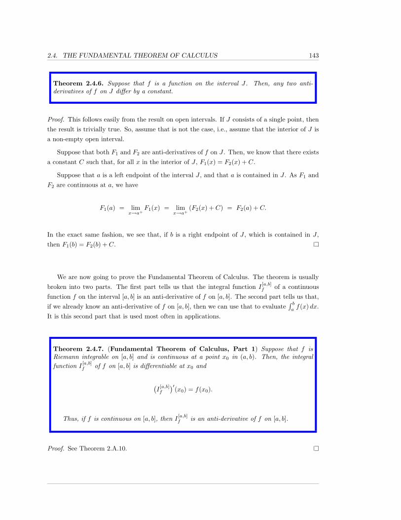
2.4. THE FUNDAMENTAL THEOREM OF CALCULUS 143
Theorem 2.4.6. Suppose that f is a function on the interval J . Then, any two anti-derivatives of f on J differ by a constant.
Proof. This follows easily from the result on open intervals. If J consists of a single point, thenthe result is trivially true. So, assume that is not the case, i.e., assume that the interior of J isa non-empty open interval.
Suppose that both F1 and F2 are anti-derivatives of f on J . Then, we know that there existsa constant C such that, for all x in the interior of J , F1(x) = F2(x) + C.
Suppose that a is a left endpoint of the interval J , and that a is contained in J . As F1 andF2 are continuous at a, we have
F1(a) = limx→a+
F1(x) = limx→a+
(F2(x) + C) = F2(a) + C.
In the exact same fashion, we see that, if b is a right endpoint of J , which is contained in J ,then F1(b) = F2(b) + C.
We are now going to prove the Fundamental Theorem of Calculus. The theorem is usuallybroken into two parts. The first part tells us that the integral function I
[a,b]f of a continuous
function f on the interval [a, b] is an anti-derivative of f on [a, b]. The second part tells us that,if we already know an anti-derivative of f on [a, b], then we can use that to evaluate
∫ baf(x) dx.
It is this second part that is used most often in applications.
Theorem 2.4.7. (Fundamental Theorem of Calculus, Part 1) Suppose that f isRiemann integrable on [a, b] and is continuous at a point x0 in (a, b). Then, the integralfunction I
[a,b]f of f on [a, b] is differentiable at x0 and
(I
[a,b]f
)′(x0) = f(x0).
Thus, if f is continuous on [a, b], then I[a,b]f is an anti-derivative of f on [a, b].
Proof. See Theorem 2.A.10.
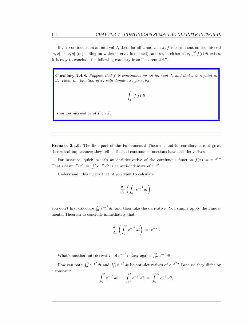
144 CHAPTER 2. CONTINUOUS SUMS: THE DEFINITE INTEGRAL
If f is continuous on an interval J , then, for all a and x in J , f is continuous on the interval[a, x] or [x, a] (depending on which interval is defined), and so, in either case,
∫ xaf(t) dt exists.
It is easy to conclude the following corollary from Theorem 2.4.7.
Corollary 2.4.8. Suppose that f is continuous on an interval J , and that a is a point inJ . Then, the function of x, with domain J , given by
∫ x
a
f(t) dt
is an anti-derivative of f on J .
Remark 2.4.9. The first part of the Fundamental Theorem, and its corollary, are of greattheoretical importance; they tell us that all continuous functions have anti-derivatives.
For instance, quick...what’s an anti-derivative of the continuous function f(x) = e−x2?
That’s easy: F (x) =∫ x
0e−t
2dt is an anti-derivative of e−x
2.
Understand: this means that, if you want to calculate
d
dx
(∫ x
0
e−t2dt
),
you don’t first calculate∫ x
0e−t
2dt, and then take the derivative. You simply apply the Funda-
mental Theorem to conclude immediately that
d
dx
(∫ x
0
e−t2dt
)= e−x
2.
What’s another anti-derivative of e−x2? Easy again:
∫ x37e−t
2dt.
How can both∫ x
0e−t
2dt and
∫ x37e−t
2dt be anti-derivatives of e−x
2? Because they differ by
a constant: ∫ x
0
e−t2dt −
∫ x
37
e−t2dt =
∫ 37
0
e−t2dt,
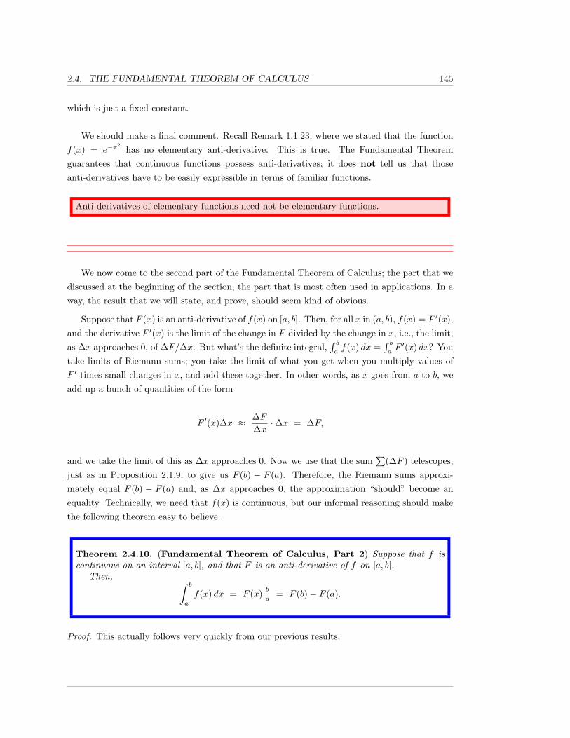
2.4. THE FUNDAMENTAL THEOREM OF CALCULUS 145
which is just a fixed constant.
We should make a final comment. Recall Remark 1.1.23, where we stated that the functionf(x) = e−x
2has no elementary anti-derivative. This is true. The Fundamental Theorem
guarantees that continuous functions possess anti-derivatives; it does not tell us that thoseanti-derivatives have to be easily expressible in terms of familiar functions.
Anti-derivatives of elementary functions need not be elementary functions.
We now come to the second part of the Fundamental Theorem of Calculus; the part that wediscussed at the beginning of the section, the part that is most often used in applications. In away, the result that we will state, and prove, should seem kind of obvious.
Suppose that F (x) is an anti-derivative of f(x) on [a, b]. Then, for all x in (a, b), f(x) = F ′(x),and the derivative F ′(x) is the limit of the change in F divided by the change in x, i.e., the limit,as ∆x approaches 0, of ∆F/∆x. But what’s the definite integral,
∫ baf(x) dx =
∫ baF ′(x) dx? You
take limits of Riemann sums; you take the limit of what you get when you multiply values ofF ′ times small changes in x, and add these together. In other words, as x goes from a to b, weadd up a bunch of quantities of the form
F ′(x)∆x ≈ ∆F∆x·∆x = ∆F,
and we take the limit of this as ∆x approaches 0. Now we use that the sum∑
(∆F ) telescopes,just as in Proposition 2.1.9, to give us F (b) − F (a). Therefore, the Riemann sums approxi-mately equal F (b) − F (a) and, as ∆x approaches 0, the approximation “should” become anequality. Technically, we need that f(x) is continuous, but our informal reasoning should makethe following theorem easy to believe.
Theorem 2.4.10. (Fundamental Theorem of Calculus, Part 2) Suppose that f iscontinuous on an interval [a, b], and that F is an anti-derivative of f on [a, b].
Then, ∫ b
a
f(x) dx = F (x)∣∣ba
= F (b)− F (a).
Proof. This actually follows very quickly from our previous results.
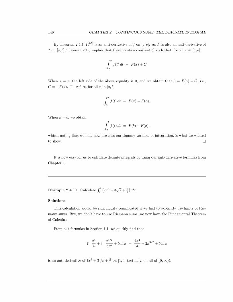
146 CHAPTER 2. CONTINUOUS SUMS: THE DEFINITE INTEGRAL
By Theorem 2.4.7, I [a,b]f is an anti-derivative of f on [a, b]. As F is also an anti-derivative of
f on [a, b], Theorem 2.4.6 implies that there exists a constant C such that, for all x in [a, b],
∫ x
a
f(t) dt = F (x) + C.
When x = a, the left side of the above equality is 0, and we obtain that 0 = F (a) + C, i.e.,C = −F (a). Therefore, for all x in [a, b],
∫ x
a
f(t) dt = F (x)− F (a).
When x = b, we obtain ∫ b
a
f(t) dt = F (b)− F (a),
which, noting that we may now use x as our dummy variable of integration, is what we wantedto show.
It is now easy for us to calculate definite integrals by using our anti-derivative formulas fromChapter 1.
Example 2.4.11. Calculate∫ 4
1
(7x3 + 3
√x+ 5
x
)dx.
Solution:
This calculation would be ridiculously complicated if we had to explicitly use limits of Rie-mann sums. But, we don’t have to use Riemann sums; we now have the Fundamental Theoremof Calculus.
From our formulas in Section 1.1, we quickly find that
7 · x4
4+ 3 · x
3/2
3/2+ 5 lnx =
7x4
4+ 2x3/2 + 5 lnx
is an anti-derivative of 7x3 + 3√x+ 5
x on [1, 4] (actually, on all of (0,∞)).
2.4. THE FUNDAMENTAL THEOREM OF CALCULUS 147
Therefore, the Fundamental Theorem tells us that
∫ 4
1
(7x3 + 3
√x+
5x
)dx =
(7x4
4+ 2x3/2 + 5 lnx
)∣∣∣∣41
=
(7 · 44
4+ 2 · 43/2 + 5 ln 4
)−(
7 · 14
4+ 2 · 13/2 + 5 ln 1
)=
448 + 16 + 5 ln 4− 74− 2− 0 =
18414
+ 5 ln 4 ≈ 467.18147.
You may be thinking “Wait – wouldn’t I get a different answer if I used a different anti-derivative of 7x3 + 3
√x+ 5
x?” The answer had better be “no”, and it is.
Any anti-derivative of 7x3 +3√x+ 5
x differs from the one we used by some constant C. Thus,the only other possibilities for us to use for the anti-derivative are all of the form
7x4
4+ 2x3/2 + 5 lnx+ C.
Does the C cause us to get a different answer? No, because when we evaluate from 1 to 4, theC gets cancelled out: (
7x4
4+ 2x3/2 + 5 lnx+ C
)∣∣∣∣41
=
(7 · 44
4+ 2 · 43/2 + 5 ln 4 + C
)−(
7 · 14
4+ 2 · 13/2 + 5 ln 1 + C
)=
(7 · 44
4+ 2 · 43/2 + 5 ln 4
)−(
7 · 14
4+ 2 · 13/2 + 5 ln 1
),
which is what we had before.
The moral of the story is that, when evaluating definite integrals by use of the FundamentalTheorem, you just use SOME anti-derivative; you don’t need to ever put in a general +C.
Example 2.4.12. Find the area under the graph of y = sinx and above the interval [0, π].
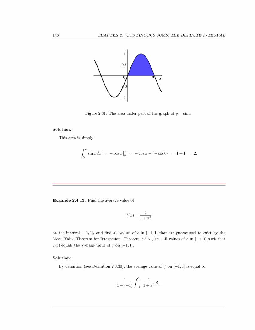
148 CHAPTER 2. CONTINUOUS SUMS: THE DEFINITE INTEGRAL
-1
-0.5
0
0.5
1
π
Figure 2.31: The area under part of the graph of y = sinx.
Solution:
This area is simply
∫ π
0
sinx dx = − cosx∣∣π0
= − cosπ − (− cos 0) = 1 + 1 = 2.
Example 2.4.13. Find the average value of
f(x) =1
1 + x2
on the interval [−1, 1], and find all values of c in [−1, 1] that are guaranteed to exist by theMean Value Theorem for Integration, Theorem 2.3.31, i.e., all values of c in [−1, 1] such thatf(c) equals the average value of f on [−1, 1].
Solution:
By definition (see Definition 2.3.30), the average value of f on [−1, 1] is equal to
11− (−1)
∫ 1
−1
11 + x2
dx.
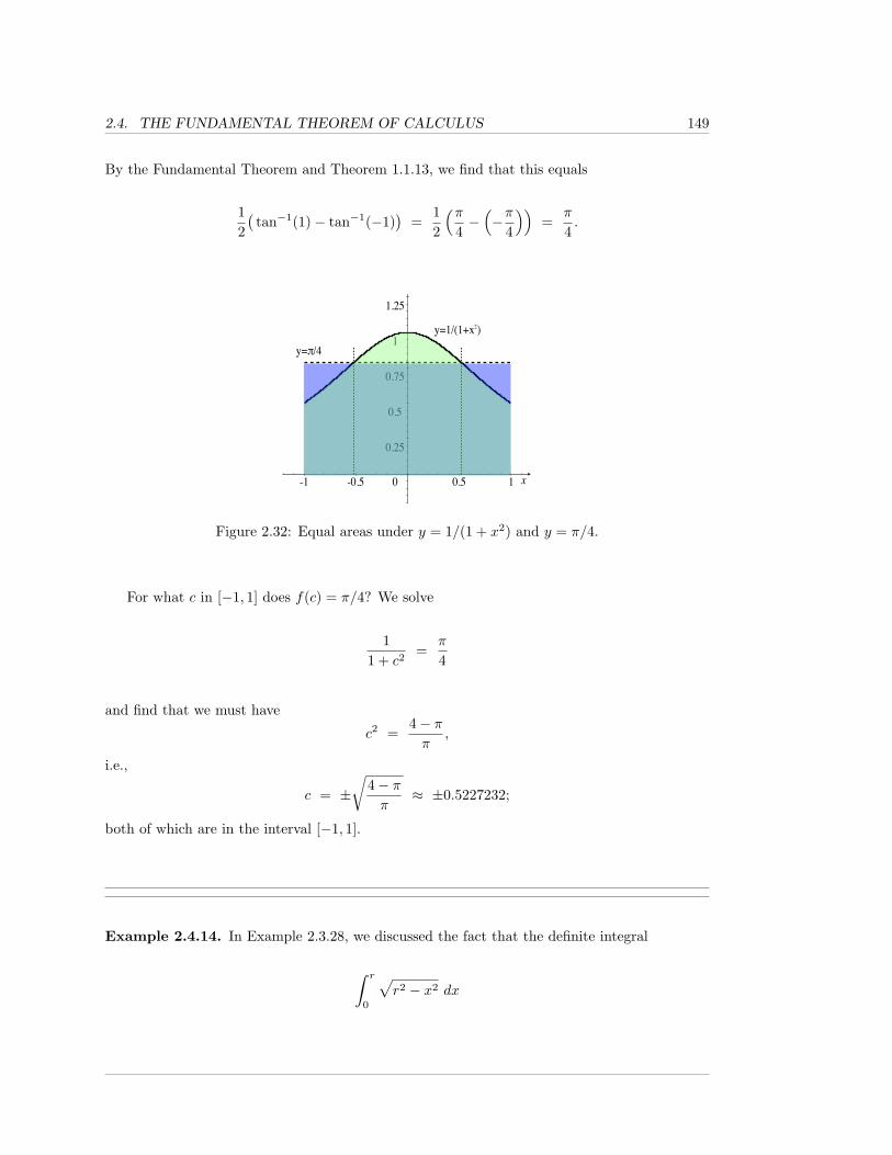
2.4. THE FUNDAMENTAL THEOREM OF CALCULUS 149
By the Fundamental Theorem and Theorem 1.1.13, we find that this equals
12(
tan−1(1)− tan−1(−1))
=12
(π4−(−π
4
))=
π
4.
-1 -0.5 0 0.5 1
-0.25
0.25
0.5
0.75
1
1.25
1.5
y=!/4
y=1/(1+x )2
y=1/(1+x )2
Figure 2.32: Equal areas under y = 1/(1 + x2) and y = π/4.
For what c in [−1, 1] does f(c) = π/4? We solve
11 + c2
=π
4
and find that we must have
c2 =4− ππ
,
i.e.,
c = ±√
4− ππ
≈ ±0.5227232;
both of which are in the interval [−1, 1].
Example 2.4.14. In Example 2.3.28, we discussed the fact that the definite integral
∫ r
0
√r2 − x2 dx
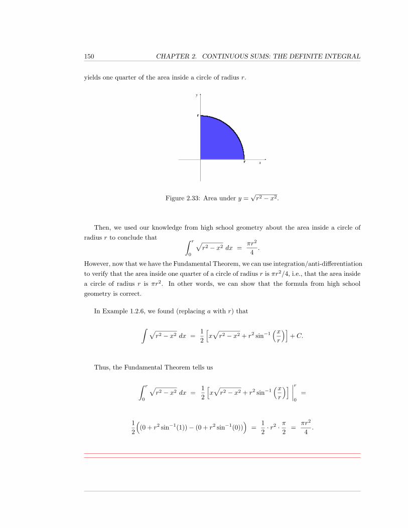
150 CHAPTER 2. CONTINUOUS SUMS: THE DEFINITE INTEGRAL
yields one quarter of the area inside a circle of radius r.
r
r
Figure 2.33: Area under y =√r2 − x2.
Then, we used our knowledge from high school geometry about the area inside a circle ofradius r to conclude that ∫ r
0
√r2 − x2 dx =
πr2
4.
However, now that we have the Fundamental Theorem, we can use integration/anti-differentiationto verify that the area inside one quarter of a circle of radius r is πr2/4, i.e., that the area insidea circle of radius r is πr2. In other words, we can show that the formula from high schoolgeometry is correct.
In Example 1.2.6, we found (replacing a with r) that
∫ √r2 − x2 dx =
12
[x√r2 − x2 + r2 sin−1
(xr
)]+ C.
Thus, the Fundamental Theorem tells us
∫ r
0
√r2 − x2 dx =
12
[x√r2 − x2 + r2 sin−1
(xr
)] ∣∣∣∣r0
=
12
((0 + r2 sin−1(1))− (0 + r2 sin−1(0))
)=
12· r2 · π
2=
πr2
4.
2.4. THE FUNDAMENTAL THEOREM OF CALCULUS 151
Substitution in Definite Integrals:
We discussed the use of substitutions in finding anti-derivatives in Theorem 1.1.15. Now thatwe have definite integration and the Fundamental Theorem, we can state a similar substitutionfor definite integrals.
Theorem 2.4.15. (Substitution in Definite Integrals) Suppose that g is continuouslydifferentiable on an open interval which contains the closed interval [a, b], and that f iscontinuous on the closed interval between the minimum and maximum values of g on [a, b].Then, ∫ b
a
f(g(x)) g′(x) dx =∫ g(b)
g(a)
f(u) du.
Proof. We will assume that g(a) ≤ g(b). The case where g(b) ≤ g(a) is essentially identical.
As f is continuous on [g(a), g(b)], f possesses an anti-derivative F on [g(a), g(b)] by Theo-rem 2.4.7, i.e., there is a function F , which is continuous on [g(a), g(b)], and such that, for all xin (g(a), g(b)), F ′(x) = f(x).
Since the composition of continuous functions is continuous, and, for all x in (a, b)
(F ◦ g)′(x) = F ′(g(x)) · g′(x),
it follows that F ◦ g is an anti-derivative of (f ◦ g) · g′ on [a, b]. The hypotheses guarantee thatf(g(x)) g′(x) is continuous on [a, b].
Therefore, we may apply the Fundamental Theorem, Theorem 2.4.10, to both sides of thedesired equality, and conclude that they are both equal to F (g(b)) − F (g(a)).
Example 2.4.16. Let’s calculate∫ 2
0xe−x
2dx in two slightly different-looking ways.
Our first method is to note that xe−x2
is continuous everywhere, and use the FundamentalTheorem, Theorem 2.4.10, to calculate the value of integral. We proceed as we did for indefiniteintegrals in Section 1.1, except that we carry along the limits of integration throughout theprocess.
Let u = −x2, so that du = −2x dx. Then, x dx = −du/2, and obtain
∫ 2
0
xe−x2dx =
∫ x=2
x=0
eu(−du/2) =−12
∫ x=2
x=0
eu du,
152 CHAPTER 2. CONTINUOUS SUMS: THE DEFINITE INTEGRAL
where we need to explicitly write x = 0 and x = 2 for the limits of integration, not just 0 and 2.
This is important: if we wrote simply∫ 2
0eu du for the integral, then the limits of inte-
gration would be telling us values of u, and then the Fundamental Theorem would give us−(e2 − 1)/2 = (1− e2)/2 for the value of the integral. This is wrong.
Proceeding correctly, we find
−12
∫ x=2
x=0
eu du =−12eu∣∣∣x=2
x=0=−12e−x
2∣∣∣20
=−e−4
2− −1
2=
1− e−4
2.
Notice that, in the above process, all that we were really doing was calculating an anti-derivative,as we did in Section 1.1, and carrying the limits of integration x = 0 and x = 2 throughout thecalculation.
What’s the other method? To apply Theorem 2.4.15, and actually change the limits ofintegration to describe what u does. This saves us cumbersome notation, and means that wedon’t need to reinsert what u was, in terms of x, at the end of the calculation. Aside from that,the process looks the same.
So, as before, let u = −x2, so that du = −2x dx. Then, of course, x dx = −du/2, but, now,we also note the values of u that we should use for the limits of integration in the u integral;when x = 0, u = −02 = 0 and, when x = 2, u = −22 = −4. Therefore, we obtain
∫ 2
0
xe−x2dx =
∫ −4
0
eu(−du/2) = =−12eu∣∣∣−4
0=−e−4
2− −1
2=
1− e−4
2.
Thus, we see that, when substituting into a definite integral, changing the limits of integrationto describe what your substitution variable is doing saves some time – maybe not a lot of time,but some.
However, there are some times when changing your limits of integration saves you a LOT
of time. Consider the integral ∫ 1
0
e−[x(x−1)]2(2x− 1) dx.
Make the substitution u = x(x − 1) = x2 − x, so that du = (2x − 1) dx. Then, the integralbecomes ∫ x=1
x=0
e−u2du.
2.4. THE FUNDAMENTAL THEOREM OF CALCULUS 153
We cannot produce a “nice” anti-derivative of e−u2; this function has no elementary anti-
derivative. See Remark 1.1.23. Nonetheless, had we changed our limits of integration to describewhat u does, we would have found that, when x = 0, u = 0, and when x = 1, u = 0; thus, ourintegral becomes ∫ 0
0
e−u2du = 0.
Therefore, in this example, switching to the u limits of integration enables us to calculate anintegral that we would not be able to calculate otherwise.
2.4.1 Exercises
In each of Exercises 1 through 15, calculate the definite integrals using the Funda-
mental Theorem of Calculus.
1.∫ 5
3
x3 + x+ 2 dx.
2.∫ 6
4
y
y2 − 3dy.
3.∫ π
2
−π2sin 3t dt.
4.∫ 200
2
5zdz.
5.∫ 6
5
√100− u2 du.
6.∫ 10
5
dw√w2 + 25
.
7.∫ 3
−3
dv
(9 + v2)2dv.
8.∫ 4
0
cosh(5y) dy.
9.∫ 3
1
8u− 35u2 − 7u
du.
10.∫ π
0
sin t cos t dt.
154 CHAPTER 2. CONTINUOUS SUMS: THE DEFINITE INTEGRAL
11.∫ 15
9
dx√x2 − 49
.
12.∫ π
0
cos2 θ dθ.
13.∫ 1
0
(2x+ 6)e(x+3)2 dx.
14.∫ 4
0
√16 + y2 dy.
15.∫ 2
0
z2 + z + 3z + 3
dz.
16. Suppose we want to calculate∫ 1
−1
dx
x. Since ln |x| is an anti-derivative of the integrand,
the Fundamental Theorem of Calculus tells us that
∫ 1
−1
dx
x= ln |x|
∣∣∣1−1
= ln 1− ln 1 = 0.
What is wrong with this argument?
17. Suppose that f is continuous on [a, b] and that G(x) =∫ x2
a
f(t) dt. What is dG/dx? Hint:
Use the Chain Rule.
In each of Exercises 18 through 22, find the average value of the function on the
closed interval if it is defined. If it is undefined, explain why.
18. k(x) =√
9− x2, [2, 5].
19. j(y) =√
1 + y2, [0, 1].
20. h(z) =1z2
, [−2, 2].
21. g(u) = coshu, [−k, k], k > 0.
22. f(v) = sec v, [0, π].
23. Find the area under the graph of y = 3ex + 2 and above the interval [0, ln 7] on the x-axis.Note that 3ex + 2 ≥ 0.
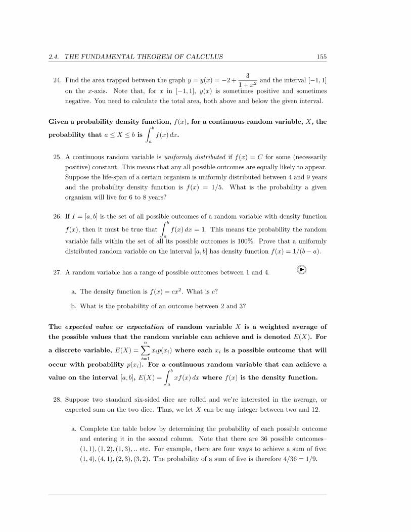
2.4. THE FUNDAMENTAL THEOREM OF CALCULUS 155
24. Find the area trapped between the graph y = y(x) = −2 +3
1 + x2and the interval [−1, 1]
on the x-axis. Note that, for x in [−1, 1], y(x) is sometimes positive and sometimesnegative. You need to calculate the total area, both above and below the given interval.
Given a probability density function, f(x), for a continuous random variable, X, the
probability that a ≤ X ≤ b is∫ b
a
f(x) dx.
25. A continuous random variable is uniformly distributed if f(x) = C for some (necessarilypositive) constant. This means that any all possible outcomes are equally likely to appear.Suppose the life-span of a certain organism is uniformly distributed between 4 and 9 yearsand the probability density function is f(x) = 1/5. What is the probability a givenorganism will live for 6 to 8 years?
26. If I = [a, b] is the set of all possible outcomes of a random variable with density function
f(x), then it must be true that∫ b
a
f(x) dx = 1. This means the probability the random
variable falls within the set of all its possible outcomes is 100%. Prove that a uniformlydistributed random variable on the interval [a, b] has density function f(x) = 1/(b− a).
27. A random variable has a range of possible outcomes between 1 and 4.
a. The density function is f(x) = cx2. What is c?
b. What is the probability of an outcome between 2 and 3?
The expected value or expectation of random variable X is a weighted average of
the possible values that the random variable can achieve and is denoted E(X). For
a discrete variable, E(X) =n∑i=1
xip(xi) where each xi is a possible outcome that will
occur with probability p(xi). For a continuous random variable that can achieve a
value on the interval [a, b], E(X) =∫ b
a
xf(x) dx where f(x) is the density function.
28. Suppose two standard six-sided dice are rolled and we’re interested in the average, orexpected sum on the two dice. Thus, we let X can be any integer between two and 12.
a. Complete the table below by determining the probability of each possible outcomeand entering it in the second column. Note that there are 36 possible outcomes–(1, 1), (1, 2), (1, 3), .. etc. For example, there are four ways to achieve a sum of five:(1, 4), (4, 1), (2, 3), (3, 2). The probability of a sum of five is therefore 4/36 = 1/9.
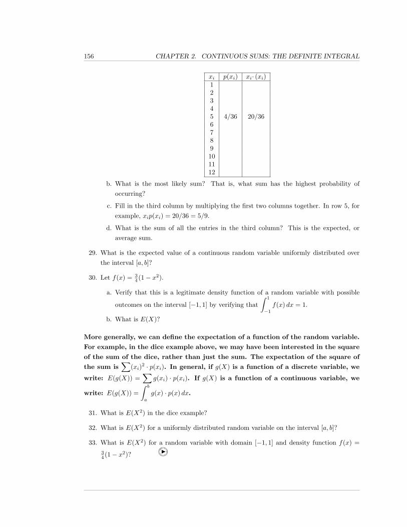
156 CHAPTER 2. CONTINUOUS SUMS: THE DEFINITE INTEGRAL
xi p(xi) xi· (xi)12345 4/36 20/366789101112
b. What is the most likely sum? That is, what sum has the highest probability ofoccurring?
c. Fill in the third column by multiplying the first two columns together. In row 5, forexample, xip(xi) = 20/36 = 5/9.
d. What is the sum of all the entries in the third column? This is the expected, oraverage sum.
29. What is the expected value of a continuous random variable uniformly distributed overthe interval [a, b]?
30. Let f(x) = 34 (1− x2).
a. Verify that this is a legitimate density function of a random variable with possible
outcomes on the interval [−1, 1] by verifying that∫ 1
−1
f(x) dx = 1.
b. What is E(X)?
More generally, we can define the expectation of a function of the random variable.
For example, in the dice example above, we may have been interested in the square
of the sum of the dice, rather than just the sum. The expectation of the square of
the sum is∑
(xi)2 · p(xi). In general, if g(X) is a function of a discrete variable, we
write: E(g(X)) =∑
g(xi) · p(xi). If g(X) is a function of a continuous variable, we
write: E(g(X)) =∫ b
a
g(x) · p(x) dx.
31. What is E(X2) in the dice example?
32. What is E(X2) for a uniformly distributed random variable on the interval [a, b]?
33. What is E(X2) for a random variable with domain [−1, 1] and density function f(x) =34 (1− x2)?
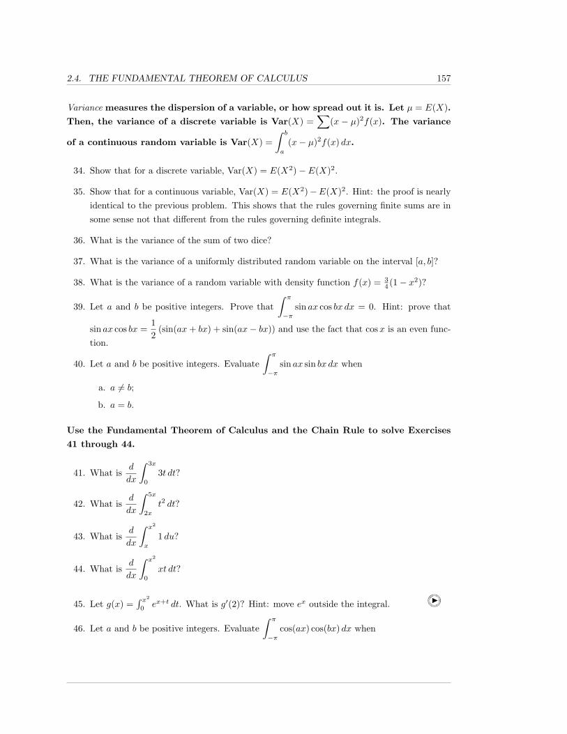
2.4. THE FUNDAMENTAL THEOREM OF CALCULUS 157
Variance measures the dispersion of a variable, or how spread out it is. Let µ = E(X).Then, the variance of a discrete variable is Var(X) =
∑(x − µ)2f(x). The variance
of a continuous random variable is Var(X) =∫ b
a
(x− µ)2f(x) dx.
34. Show that for a discrete variable, Var(X) = E(X2)− E(X)2.
35. Show that for a continuous variable, Var(X) = E(X2)−E(X)2. Hint: the proof is nearlyidentical to the previous problem. This shows that the rules governing finite sums are insome sense not that different from the rules governing definite integrals.
36. What is the variance of the sum of two dice?
37. What is the variance of a uniformly distributed random variable on the interval [a, b]?
38. What is the variance of a random variable with density function f(x) = 34 (1− x2)?
39. Let a and b be positive integers. Prove that∫ π
−πsin ax cos bx dx = 0. Hint: prove that
sin ax cos bx =12
(sin(ax+ bx) + sin(ax− bx)) and use the fact that cosx is an even func-tion.
40. Let a and b be positive integers. Evaluate∫ π
−πsin ax sin bx dx when
a. a 6= b;
b. a = b.
Use the Fundamental Theorem of Calculus and the Chain Rule to solve Exercises
41 through 44.
41. What isd
dx
∫ 3x
0
3t dt?
42. What isd
dx
∫ 5x
2x
t2 dt?
43. What isd
dx
∫ x2
x
1 du?
44. What isd
dx
∫ x2
0
xt dt?
45. Let g(x) =∫ x2
0ex+t dt. What is g′(2)? Hint: move ex outside the integral.
46. Let a and b be positive integers. Evaluate∫ π
−πcos(ax) cos(bx) dx when
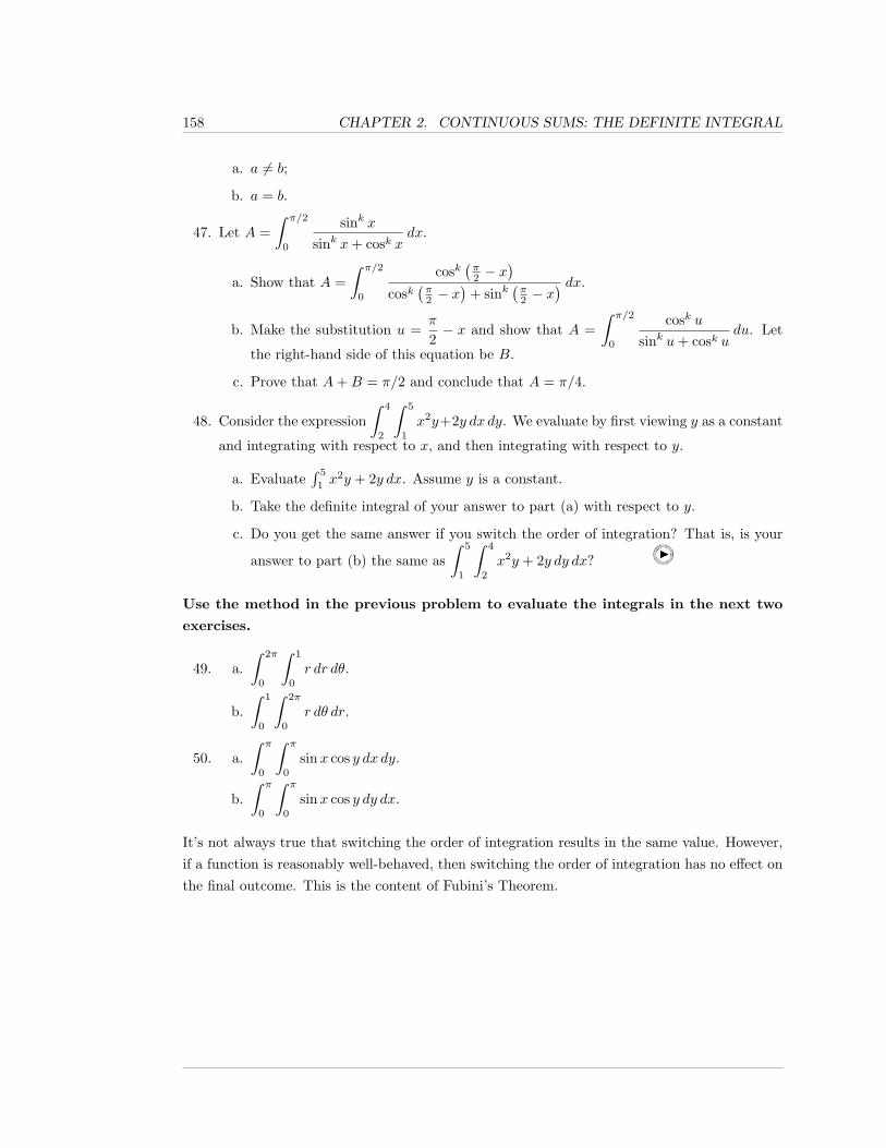
158 CHAPTER 2. CONTINUOUS SUMS: THE DEFINITE INTEGRAL
a. a 6= b;
b. a = b.
47. Let A =∫ π/2
0
sink xsink x+ cosk x
dx.
a. Show that A =∫ π/2
0
cosk(π2 − x
)cosk
(π2 − x
)+ sink
(π2 − x
) dx.
b. Make the substitution u =π
2− x and show that A =
∫ π/2
0
cosk usink u+ cosk u
du. Let
the right-hand side of this equation be B.
c. Prove that A+B = π/2 and conclude that A = π/4.
48. Consider the expression∫ 4
2
∫ 5
1
x2y+2y dx dy. We evaluate by first viewing y as a constant
and integrating with respect to x, and then integrating with respect to y.
a. Evaluate∫ 5
1x2y + 2y dx. Assume y is a constant.
b. Take the definite integral of your answer to part (a) with respect to y.
c. Do you get the same answer if you switch the order of integration? That is, is your
answer to part (b) the same as∫ 5
1
∫ 4
2
x2y + 2y dy dx?
Use the method in the previous problem to evaluate the integrals in the next two
exercises.
49. a.∫ 2π
0
∫ 1
0
r dr dθ.
b.∫ 1
0
∫ 2π
0
r dθ dr.
50. a.∫ π
0
∫ π
0
sinx cos y dx dy.
b.∫ π
0
∫ π
0
sinx cos y dy dx.
It’s not always true that switching the order of integration results in the same value. However,if a function is reasonably well-behaved, then switching the order of integration has no effect onthe final outcome. This is the content of Fubini’s Theorem.
2.5. IMPROPER INTEGRALS 159
2.5 Improper Integrals
In this section, we will define the integral of a function over a set of real numbers, where the setof real numbers need not be a closed, bounded, interval; we also define integrals when the valueof the integrand is unbounded, even if the interval of integration is itself bounded. This reallyrequires a new definition, for Theorem 2.3.6 tells us that the Riemann integral of an unboundedfunction does not exist.
The actual calculation of our new type of integral will involve calculating our usual integralson intervals of the form [a, b], where now either a or b varies, and we will then take a limitas a or b approaches some “problematic” value. Of course, the calculation of the integrals onthe intervals [a, b] can/will still use the Fundamental Theorem of Calculus, and, hence, we mayapply all of our techniques from earlier sections to find anti-derivatives.
As we wish to be able to discuss integrals over intervals [a, b] and over intervals (a, b] (andover other sets), the notation
∫ ba
does not suffice to distinguish between the types of intervalsthat we care about. Thus, we adopt some new notation; if E is a subset of the real numbers,we will write ∫
E
f(x) dx
for the integral of f over the set E. Of course, right now, this has no meaning for us, unless Eis a closed interval [a, b], in which case
∫ baf(x) dx =
∫[a,b]
f(x) dx. Our goal in this section is todefine
∫Ef(x) dx for sets E that need not be closed intervals.
Before we really start looking at new types of integrals, it will be helpful to have a new pieceof terminology.
Definition 2.5.1. If f is a real function, with domain D, an extension of f is a functionf whose domain is larger (or equal to) D, and such that f and f agree at all points of D,i.e., for all x in D, f(x) = f(x).
In other words, an extension f , of f , is a function whose domain includes the domain,D, of f , and such that the restriction of f to D is equal to f .
160 CHAPTER 2. CONTINUOUS SUMS: THE DEFINITE INTEGRAL
Example 2.5.2. For example, the function f , with domain [0, 1] given by
f =
sinxx
if 0 < x ≤ 1;
1 if x = 0
is an extension of the function f(x) = (sinx)/x, with domain (0, 1]. In fact, f is a continuous
extension of f to [0, 1], since
limx→0+
sinxx
= 1.
Now, let’s start our discussion of more general notions of integration by looking at the easiestcase, one where we already know the answer: the case of a function which is Riemann integrable.
Example 2.5.3. Consider f(x) = x2 on the interval [0, 1]. Certainly, f is Riemann integrable on[0, 1], since f is continuous on [0, 1]. Thus, we know what
∫[0,1]
x2 dx means; it means∫ 1
0x2 dx,
which, by the Fundamental Theorem of Calculus, is equal to (x3/3)∣∣10
= 1/3.
What if we omit the 0 from the interval of integration, i.e., what should∫
(0,1]x2 dx mean?
Theorem 2.3.14 tells us that, for Riemann integrals on closed intervals, altering the function ata finite number of points does not change the integrability of the function or the value of theintegral. Thus, intuitively, it seems reasonable that omitting a single point of integration, like 0,should not affect the integral. Therefore, in this case, it seems reasonable to make the definitionthat ∫
(0,1]
x2 dx =∫
[0,1]
x2 dx =13.
While this seems reasonable, it should, in a way, seem like “cheating”; we wanted to integratef(x) = x2 on the interval (0, 1], and yet we used information about f on the larger interval [0, 1],i.e., we used that there was a continuous extension of f from the interval (0, 1] to the interval[0, 1]. Could we have defined
∫(0,1]
x2 dx without using the extension to [0, 1]? Yes.
For all a such that 0 < a ≤ 1, f(x) = x2 is Riemann integrable on the interval [a, 1], and
∫ 1
a
x2 dx =x3
3
∣∣∣1a
=13− a3
3,
and this integral uses only that f(x) = x2 is defined on (0, 1].
2.5. IMPROPER INTEGRALS 161
Now, we can take the limit as a approached 0 from the right to obtain our previous answer.That is, we could have defined
∫(0,1]
x2 dx by
∫(0,1]
x2 dx = lima→0+
∫ 1
a
x2 dx = lima→0+
(13− a3
3
)=
13.
The point is that, in this example, we obtain the same value for∫
(0,1]x2 dx, regardless of
whether we use the fact that x2 extends to [0, 1] or whether we instead use the limits of integrals,as our lower-limit of integration approaches 0.
Example 2.5.4. Let’s consider a more-complicated example. Let f be the function, withdomain (0, 1], given by
f(x) =sinxx
.
How many choices do we have for reasonable ways to define the integral∫
(0,1]f(x) dx? At least
two.
First, we can define an extension f to the closed interval [0, 1], and then define
∫(0,1]
sinxx
dx =∫
[0,1]
f(x) dx.
Of course, we either need to pick a particular extension, or show that the value of∫
[0,1]f(x) dx
is always the same, regardless of what extension we select. We could, in fact, take f to be thecontinuous extension of f given in Example 2.5.2; then, f would certainly be Riemann integrableby Theorem 2.3.8.
However, we don’t have to use continuous extension of f . Since (sinx)/x does possessa continuous extension to the interval [0, 1], it follows that (sinx)/x is bounded on (0, 1]. Thus,Theorem 2.3.8 and Theorem 2.3.14 imply that it doesn’t matter how we define f at x = 0; nomatter what value we chose for f(0), f will be bounded and, at least, piecewise-continuous –hence, Riemann integrable – and changing the value at one point will not affect the value of theintegral. Therefore, we could define
∫(0,1]
f(x) dx =∫
[0,1]
f dx,
162 CHAPTER 2. CONTINUOUS SUMS: THE DEFINITE INTEGRAL
for any extension of f to a function f on [0, 1].
However, we could take the second approach, as we did in Example 2.5.3; without using anextension at all, we could define
∫(0,1]
sinxx
dx = lima→0+
∫ 1
a
sinxx
dx.
This leads to a new question or two. If 0 < a ≤ 1, we know that (sinx)/x is continuous on [a, 1]and, hence,
∫ 1
asin xx dx exists. But, how do we know that the limit as a → 0+ exists and, even
if the limit does exist, how do we know that that limit is equal to what we’d get by extending(sinx)/x to [0, 1] and then taking the Riemann integral of our extension over [0, 1]?
Actually, the answers to these questions are easy, given our earlier results. Suppose that fis an extension of f to [0, 1]. Then, as we discussed above, f is Riemann integrable on [0, 1]. ByRemark 2.4.4, the function on [0, 1] that sends a to
∫ 1
af(x) dx is continuous; in particular,
∫ 1
0
f(x) dx = lima→0+
∫ 1
a
f(x) dx = lima→0+
∫ 1
a
f(x) dx,
where the second equality above follows from the fact that, if 0 < x ≤ 1, then f(x) = f(x),since f is an extension of f .
Thus, lima→0+
∫ 1
af(x) dx exists and equals what we would obtain by calculating the Riemann
integral of any extension of f to [0, 1]. Therefore, it seems reasonable to define the integral of fover the half-open interval (0, 1] by
∫(0,1]
sinxx
dx = lima→0+
∫ 1
a
sinxx
dx.
What we have seen in the previous two examples is that, in those cases, it made sense todefine
∫(0,1]
f(x) dx by ∫(0,1]
f(x) dx = lima→0+
∫ 1
a
f(x) dx,
where each∫ 1
af(x) dx is a Riemann integral. However, in those cases, we could also have defined∫
(0,1]f(x) dx by extending f to the closed interval [0, 1] and then using the Riemann integral of
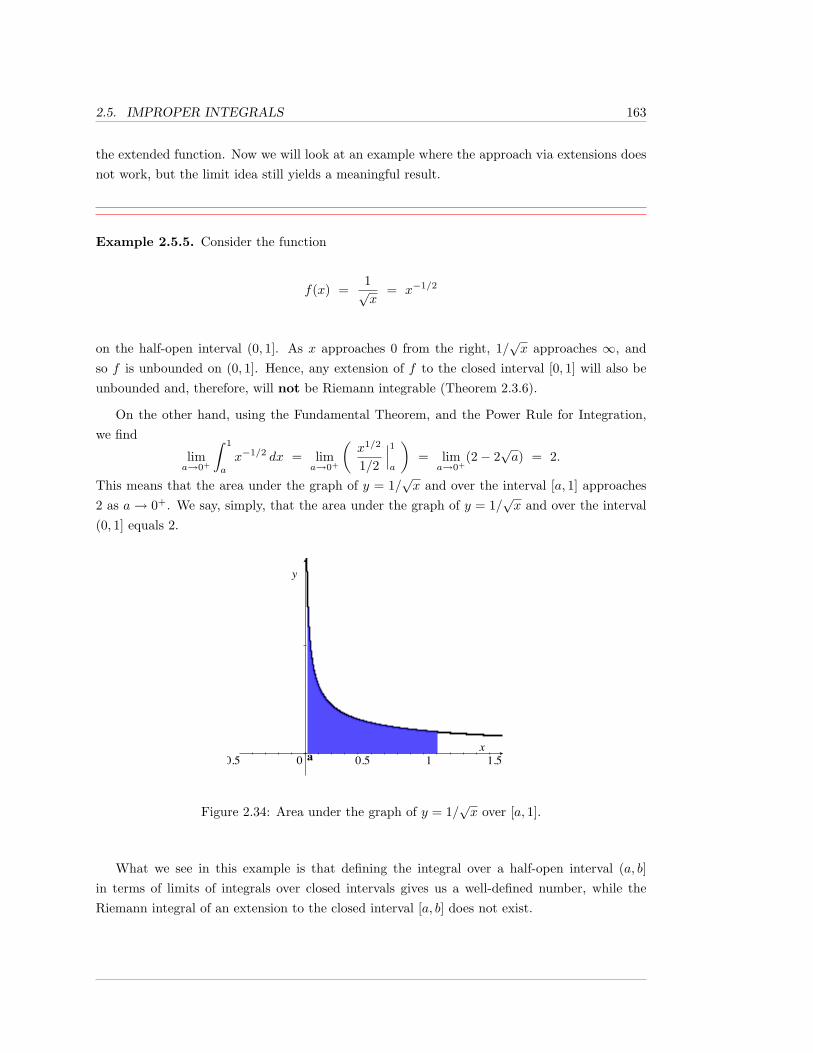
2.5. IMPROPER INTEGRALS 163
the extended function. Now we will look at an example where the approach via extensions doesnot work, but the limit idea still yields a meaningful result.
Example 2.5.5. Consider the function
f(x) =1√x
= x−1/2
on the half-open interval (0, 1]. As x approaches 0 from the right, 1/√x approaches ∞, and
so f is unbounded on (0, 1]. Hence, any extension of f to the closed interval [0, 1] will also beunbounded and, therefore, will not be Riemann integrable (Theorem 2.3.6).
On the other hand, using the Fundamental Theorem, and the Power Rule for Integration,we find
lima→0+
∫ 1
a
x−1/2 dx = lima→0+
(x1/2
1/2
∣∣∣1a
)= lim
a→0+(2− 2
√a) = 2.
This means that the area under the graph of y = 1/√x and over the interval [a, 1] approaches
2 as a→ 0+. We say, simply, that the area under the graph of y = 1/√x and over the interval
(0, 1] equals 2.
-0.5 0 0.5 1 1.5a
Figure 2.34: Area under the graph of y = 1/√x over [a, 1].
What we see in this example is that defining the integral over a half-open interval (a, b]in terms of limits of integrals over closed intervals gives us a well-defined number, while theRiemann integral of an extension to the closed interval [a, b] does not exist.
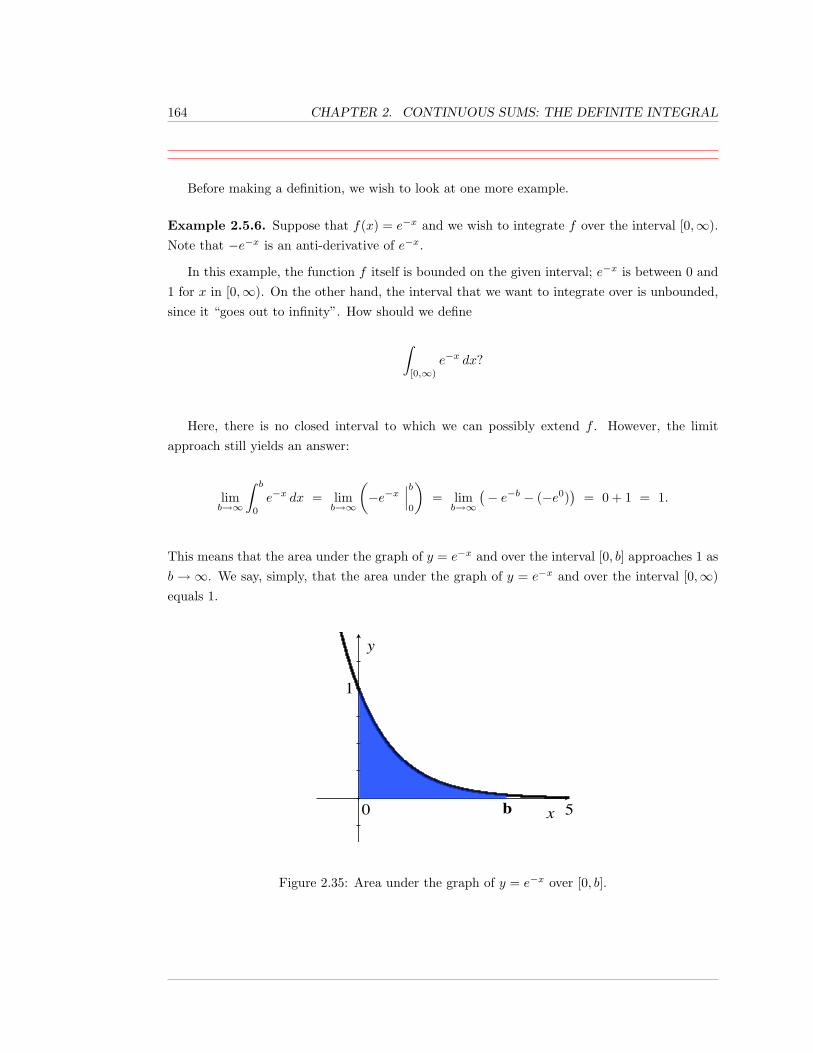
164 CHAPTER 2. CONTINUOUS SUMS: THE DEFINITE INTEGRAL
Before making a definition, we wish to look at one more example.
Example 2.5.6. Suppose that f(x) = e−x and we wish to integrate f over the interval [0,∞).Note that −e−x is an anti-derivative of e−x.
In this example, the function f itself is bounded on the given interval; e−x is between 0 and1 for x in [0,∞). On the other hand, the interval that we want to integrate over is unbounded,since it “goes out to infinity”. How should we define
∫[0,∞)
e−x dx?
Here, there is no closed interval to which we can possibly extend f . However, the limitapproach still yields an answer:
limb→∞
∫ b
0
e−x dx = limb→∞
(−e−x
∣∣∣b0
)= lim
b→∞
(− e−b − (−e0)
)= 0 + 1 = 1.
This means that the area under the graph of y = e−x and over the interval [0, b] approaches 1 asb → ∞. We say, simply, that the area under the graph of y = e−x and over the interval [0,∞)equals 1.
0 5
1
b
Figure 2.35: Area under the graph of y = e−x over [0, b].
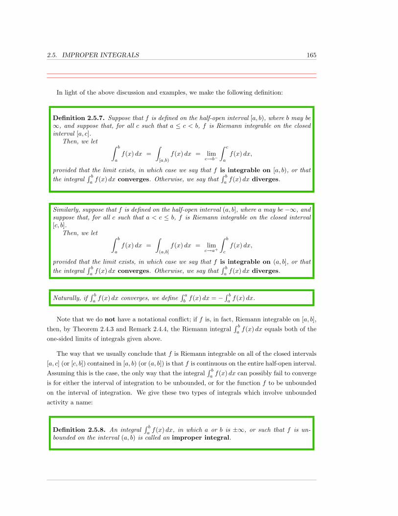
2.5. IMPROPER INTEGRALS 165
In light of the above discussion and examples, we make the following definition:
Definition 2.5.7. Suppose that f is defined on the half-open interval [a, b), where b may be∞, and suppose that, for all c such that a ≤ c < b, f is Riemann integrable on the closedinterval [a, c].
Then, we let ∫ b
a
f(x) dx =∫
[a,b)
f(x) dx = limc→b−
∫ c
a
f(x) dx,
provided that the limit exists, in which case we say that f is integrable on [a, b), or thatthe integral
∫ baf(x) dx converges. Otherwise, we say that
∫ baf(x) dx diverges.
Similarly, suppose that f is defined on the half-open interval (a, b], where a may be −∞, andsuppose that, for all c such that a < c ≤ b, f is Riemann integrable on the closed interval[c, b].
Then, we let ∫ b
a
f(x) dx =∫
(a,b]
f(x) dx = limc→a+
∫ b
c
f(x) dx,
provided that the limit exists, in which case we say that f is integrable on (a, b], or thatthe integral
∫ baf(x) dx converges. Otherwise, we say that
∫ baf(x) dx diverges.
Naturally, if∫ baf(x) dx converges, we define
∫ abf(x) dx = −
∫ baf(x) dx.
Note that we do not have a notational conflict; if f is, in fact, Riemann integrable on [a, b],then, by Theorem 2.4.3 and Remark 2.4.4, the Riemann integral
∫ baf(x) dx equals both of the
one-sided limits of integrals given above.
The way that we usually conclude that f is Riemann integrable on all of the closed intervals[a, c] (or [c, b]) contained in [a, b) (or (a, b]) is that f is continuous on the entire half-open interval.Assuming this is the case, the only way that the integral
∫ baf(x) dx can possibly fail to converge
is for either the interval of integration to be unbounded, or for the function f to be unboundedon the interval of integration. We give these two types of integrals which involve unboundedactivity a name:
Definition 2.5.8. An integral∫ baf(x) dx, in which a or b is ±∞, or such that f is un-
bounded on the interval (a, b) is called an improper integral.
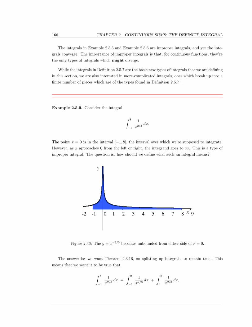
166 CHAPTER 2. CONTINUOUS SUMS: THE DEFINITE INTEGRAL
The integrals in Example 2.5.5 and Example 2.5.6 are improper integrals, and yet the inte-grals converge. The importance of improper integrals is that, for continuous functions, they’rethe only types of integrals which might diverge.
While the integrals in Definition 2.5.7 are the basic new types of integrals that we are definingin this section, we are also interested in more-complicated integrals, ones which break up into afinite number of pieces which are of the types found in Definition 2.5.7 .
Example 2.5.9. Consider the integral
∫ 8
−1
1x2/3
dx.
The point x = 0 is in the interval [−1, 8], the interval over which we’re supposed to integrate.However, as x approaches 0 from the left or right, the integrand goes to ∞. This is a type ofimproper integral. The question is: how should we define what such an integral means?
-2 -1 0 1 2 3 4 5 6 7 8 9
Figure 2.36: The y = x−2/3 becomes unbounded from either side of x = 0.
The answer is: we want Theorem 2.3.16, on splitting up integrals, to remain true. Thismeans that we want it to be true that
∫ 8
−1
1x2/3
dx =∫ 0
−1
1x2/3
dx +∫ 8
0
1x2/3
dx,
2.5. IMPROPER INTEGRALS 167
where each of the summands on the right is an integral of the type we defined in Definition 2.5.7.We now calculate by taking limits:
limb→0−
∫ b
−1
x−2/3 dx + lima→0+
∫ 8
a
x−2/3 dx = limb→0−
(3x1/3
∣∣b−1
)+ lim
a→0+
(3x1/3
∣∣8a
)=
limb→0−
(3b1/3 − 3(−1)1/3
)+ lim
a→0+
(3(8)1/3 − 3a1/3
)= 3 + 6 = 9.
There can also be multiple “problem points”.
Example 2.5.10. Consider the integral
∫ ∞1
1(x− 2)(x− 4)
dx.
After possibly removing a finite number of points (problem points, where unboundednesscomes into play), we want to split the interval [1,∞) into a finite number of closed or half-openintervals on which the integrand 1/[(x − 2)(x − 4)] is continuous; in this splitting, we allow apair of closed or half-open intervals to intersect each other in, at most, one point. We then addtogether the resulting integrals, provided all of them exist; otherwise, we say that the originalintegral diverges.
Thus, we start with the interval [1,∞). We remove the two points x = 2 and x = 4, where1/[(x − 2)(x − 4)] is undefined. For now, this gives us intervals [1, 2), (2, 4), and (4,∞). Theintervals (2, 4) and (4,∞) are not closed or half-open. Why do we care? We do not want tohave to deal with some sort of simultaneous limits at the two endpoints of the intervals.
Therefore, we further split the intervals (2, 4), and (4,∞). Where do we split them? At anypoint in-between the endpoints. It is a theorem, which we incorporated into the statement ofDefinition 2.5.11, that is doesn’t matter where the splitting occurs. So, we split the interval(2, 4) into (2, 2.5] and [2.5, 4) (pairs of half-open intervals may intersect at a point), and we split(4,∞) into (4, 7] and [7,∞).
We end up with five half-open intervals: I1 = [1, 2), I2 = (2, 2.5], I3 = [2.5, 4), I4 = (4, 7],and I5 = [7,∞), whose union is equal to the original interval [1,∞), minus a finite number ofpoints, and pairs of the half-open intervals intersect each other in, at most, one point.
168 CHAPTER 2. CONTINUOUS SUMS: THE DEFINITE INTEGRAL
Now, we define ∫ ∞1
1(x− 2)(x− 4)
dx
to equal the sum
∫I1
1(x− 2)(x− 4)
dx +∫I2
1(x− 2)(x− 4)
dx +∫I3
1(x− 2)(x− 4)
dx +
∫I4
1(x− 2)(x− 4)
dx +∫I5
1(x− 2)(x− 4)
dx,
provided that all of these integrals exist, in which case we say that∫∞
11
(x−2)(x−4) dx converges.If one (or more) of the five separate integrals, appearing in the summation, diverges, then wesay that
∫∞1
1(x−2)(x−4) dx diverges.
In the remainder of this example, we will show that
∫ ∞1
1(x− 2)(x− 4)
dx
diverges, by showing that the first improper integral in the summation above diverges, i.e., wewill show that ∫ 2
1
1(x− 2)(x− 4)
dx = limb→2−
∫ b
1
1(x− 2)(x− 4)
dx
diverges to ∞.
We find an anti-derivative of 1(x−2)(x−4) via partial fractions, as in Section 1.3. So, we first
determine constants A and B such that
1(x− 2)(x− 4)
=A
x− 2+
B
x− 4,
for all x, other than x = 2 and x = 4. Clearing the denominators, by multiplying each side ofthe equality by the big denominator on the left, i.e., by (x− 2)(x− 4), we obtain
1 = A(x− 4) + B(x− 2),
which needs to hold for all x. Plugging in x = 2, we find that 1 = A · (−2) + B · 0, so that
2.5. IMPROPER INTEGRALS 169
A = −1/2. Plugging in x = 4, we find that 1 = A · 0 +B · 2, and so B = 1/2. Thus,
1(x− 2)(x− 4)
=−1/2x− 2
+1/2x− 4
,
and we want to calculate
limb→2−
∫ b
1
1(x− 2)(x− 4)
dx = limb→2−
∫ b
1
(−1/2x− 2
+1/2x− 4
)dx, (2.3)
or show that it doesn’t exist. We need to find an anti-derivative of 1/(x− a), where a is 2 or 4.We accomplish this by making the substitution u = x− a, so that du = dx, and
∫1
x− adx =
∫1udu = ln |u| + C = ln |x− a| + C.
Thus, Formula 2.3 becomes
limb→2−
∫ b
1
1(x− 2)(x− 4)
dx = limb→2−
(−12
ln |x− 2|+ 12
ln |x− 4|)∣∣∣∣b
1
.
As b is approaching 2 from the left, we know that all of the x’s that we are considering are lessthan 2 and, hence, |x−2| = 2−x and |x−4| = 4−x. Now, evaluating at x = b and subtractingthe value at x = 1, we find
limb→2−
∫ b
1
1(x− 2)(x− 4)
dx = limb→2−
(−12
ln(2− b) +12
ln(4− b)− 12
ln 3),
where we used that ln 1 = 0. As b approaches 2 from the left, 12 ln(4 − b) − 1
2 ln 3 approaches12 ln 2− 1
2 ln 3, but −12 ln(2− b) approaches (−1/2)(−∞) =∞.
Therefore,∫ 2
11
(x−2)(x−4) dx diverges, and so does the integral over the bigger interval [1,∞).
We should mention that, just because∫ 2
11
(x−2)(x−4) dx diverges to ∞, that does not imply that∫∞1
1(x−2)(x−4) dx also diverges to ∞; other parts of the summand that we split the integral into
may (and do) diverge to −∞. Thus, we simply say that∫∞
11
(x−2)(x−4) dx diverges, withouttrying to specify the manner in which it diverges.
170 CHAPTER 2. CONTINUOUS SUMS: THE DEFINITE INTEGRAL
We summarize our discussion and example above into a definition. In this definition, we willsplit a set into a union of closed or half-open intervals (as we did above); the point is that eachof the intervals that we split things into has a “problem”, an unboundedness issue, at, at most,one endpoint. It is important that the definition gives you the same result, regardless of howyou pick the half-open intervals. The proof of this is in Theorem 2.A.11.
Definition 2.5.11. Let E be a subset of the real numbers which is the union of a finitenumber of intervals. Let f be a real function, which is defined and continuous on the set Eexcept, perhaps, at a finite set of points P . Let E − P denote the set of points in E whichare not in the set P .
Then, E−P is a union of a finite number of closed or half-open intervals I1, I2, . . . , In onwhich f is defined and continuous. Given any such decomposition of E − P into intervals,we define the integral of f on E by
∫E
f(x) dx =∫I1
f(x) dx +∫I2
f(x) dx + . . . +∫In
f(x) dx,
provided that each integral in the summation on the right converges; in this case, we saythat
∫Ef(x) dx converges or that f is integrable on E. If any one of the integrals in the
summation above diverges, then we say that∫Ef(x) dx diverges.
These definitions of converges, diverges, and the value of the integral are independent of thechoice of the intervals I1, I2, . . . , In, as long as the given conditions are satisfied.
If E is an interval [a, b], [a, b), (a, b], or (a, b), then we may also use other notation; we set
∫ b
a
f(x) dx =∫E
f(x) dx, and∫ a
b
f(x) dx = −∫E
f(x) dx.
Note that, with our terminology, we may say that a function f is integrable on a set E,even if f is not defined at a finite number of the points in E. For instance, inExample 2.5.9, we would say that 1/x2/3 is integrable on (−1, 8), even though 1/x2/3 is notdefined at x = 0. Be aware that other books might use different terminology, and might notsay that f is integrable on a set on which f is not defined.
2.5. IMPROPER INTEGRALS 171
Just as we have linearity for Riemann integrals, Theorem 2.3.19, we also have linearity forour more general integrals, provided the individual integrals converge. The proof is essentiallyidentical, except that, to deal with the improper integrals, you must use that limits are “linear”,i.e., you can pull constants out of limits and split up sums.
Theorem 2.5.12. (Linearity of Improper Integrals) Let E be a subset of the realnumbers which is the union of a finite number of intervals. Suppose that f and g areintegrable on E, and that a and b are any real numbers. Then, af + bg is integrable on Eand ∫
E
af(x) + bg(x) dx = a
∫E
f(x) dx + b
∫E
g(x) dx.
Example 2.5.13. As we saw in Example 2.5.5 and Example 2.5.9 (with different upper-limitsof integration), the integrals
∫ 1
0
1x1/2
dx and∫ 1
0
1x2/3
dx
both converge; we leave it as an exercise for you to show that they converge to 2 and 3, respec-tively.
Therefore, ∫ 1
0
(5
x1/2− 7
x2/3
)dx
converges, and equals 5 · 2− 7 · 3 = −11.
It is sometimes possible to tell that an improper integral converges, without being able todetermine what it converges to. This seemingly bizarre fact stems from a defining propertyof the real numbers: every non-empty set of real numbers, which has an upper bound, has aLEAST upper bound. See Definition 5.1.15 and Theorem 5.1.18. This least upper bound propertyis the main reason that we can sometimes tell that limits, as in improper integrals, exist withoutknowing the value.
We first give a theorem which says that there’s only one way for some types of improperintegrals to diverge.
172 CHAPTER 2. CONTINUOUS SUMS: THE DEFINITE INTEGRAL
Theorem 2.5.14. Let I be an interval of the form [a, b) or (a, b], where we allow theintervals [a,∞) or (−∞, b]. Suppose that, for all x in I, f(x) ≥ 0, and that, for all closedintervals [c, d] contained in I, f is Riemann integrable on [c, d].
Then, if there exists a real number M (an upper bound) such that, for all [c, d] containedin I,
∫ dcf(x) dx ≤ M , then
∫ baf(x) dx converges, and what it converges to is less than, or
equal to, M ; in other words, if there is an upper bound M on all of the∫ dcf(x) dx, then∫ b
af(x) dx converges to the least such upper bound.
In particular, if∫ baf(x) dx diverges, what it diverges to is ∞.
Proof. See Theorem 2.A.12.
Remark 2.5.15. The analogous statement for f(x) ≤ 0 is true, and is obtained by applyingTheorem 2.5.14 to −f(x), which would be non-negative.
What you find for non-positive f is: if there exists a real number M (a lower-bound) suchthat, for all [c, d] contained in I, M ≤
∫ dcf(x) dx, then
∫ baf(x) dx converges to the greatest such
lower bound. In particular, if∫ baf(x) dx diverges, what it diverges to is −∞.
Corollary 2.5.16. Let I be an interval of the form [a, b) or (a, b], where we allow theintervals [a,∞) or (−∞, b]. Suppose that, for all x in I, 0 ≤ f(x) ≤ g(x), and that, for allclosed intervals [c, d] contained in I, f and g are Riemann integrable on [c, d].
Then, if∫ bag(x) dx converges, then so does
∫ baf(x) dx, and what it converges to is some-
thing less than, or equal to,∫ bag(x) dx. This implies that, if
∫ baf(x) dx diverges, then so
does∫ bag(x) dx.
Proof. This is easy now. Since f ≤ g on I, Theorem 2.3.20 tells us that, for all [c, d] containedin I, ∫ d
c
f(x) dx ≤∫ d
c
g(x) dx.
If∫ bag(x) dx converges, then Theorem 2.5.14 tells us that it converges to the least upper bound
M on the integrals∫ dcg(x) dx, but, by the inequality above, this M is an upper bound on all of
the integrals∫ dcf(x) dx. The corollary now follows by applying Theorem 2.5.14 again.
2.5. IMPROPER INTEGRALS 173
Example 2.5.17. Consider the integrals
∫ 1
0
1 + sinx√x
dx and∫ ∞
1
2 + sinxx
dx.
Producing manageable anti-derivatives of these integrands is problematic/impossible. Nonethe-less, we can use Corollary 2.5.16 to determine quickly whether they converge or not.
First, note that, for all x in (0, 1],
0 ≤ 1 + sinx√x
≤ 2√x,
and that, for all x in [1,∞),
0 ≤ 1x≤ 2 + sinx
x.
Now, we find
∫ 1
0
2√xdx = lim
a→0+
∫ 1
a
2√xdx = lim
a→0+4x1/2
∣∣∣1a
= 4 · lima→0+
(1− a1/2) = 4,
and ∫ ∞1
1xdx = lim
b→∞(ln b− ln 1) = ∞.
Combining all of the above with Corollary 2.5.16, we conclude that∫ 1
0
1 + sinx√x
dx converges
(to something less than or equal to 4, but we don’t know what), while∫ ∞
1
2 + sinxx
dx diverges
to ∞.
2.5.1 Exercises
In Exercises 1 through 17, evaluate the given integral if it converges; otherwise,
show that the integral diverges.
174 CHAPTER 2. CONTINUOUS SUMS: THE DEFINITE INTEGRAL
1.∫ ∞
0
dx
(2x+ 5)2.
2.∫ ∞
1
dt
(4 + 5t)3/2.
3.∫ ∞
0
dx
7x− 5.
4.∫ ∞
1
dy
(4y − 3)1/2.
5.∫ ∞
0
sin z dz.
6.∫ ∞
0
du
(u+ 3)(u+ 5).
7.∫ ∞−4
du
(u+ 3)(u+ 5).
8.∫ π
0
dv
1− cos v. Hint: use a half-angle identity to evaluate the integral.
9.∫ 1
0
dt√1− t2
.
10.∫ ∞
0
dw
1 + w2.
11.∫ 1
0
x−1/2 lnx dx.
12.∫ 1
0
x−2 lnx dx.
13.∫ k
−k
dt3√tdt, k > 0.
14.∫ ∞
0
tan−1 z
1 + z2dz.
15. Let n > 1. Does∫ 1
0
dx
xnconverge or diverge? If it converges, what does it converge to?
16. Let n = 1. Does∫ 1
0
dx
xnconverge or diverge? If it converges, what does it converge to?
17. Let n < 1. Does∫ 1
0
dx
xnconverge or diverge? If it converges, what does it converge to?
2.5. IMPROPER INTEGRALS 175
Use Corollary 2.5.16 to determine whether the integrals in Exercises 18 through 24
converge or diverge. If they converge, you need not calculate the integrals.
18.∫ ∞−∞
11 + x6
dx.
19.∫ ∞
2
| sinx|1 + x2
dx.
20.∫ ∞
1
et
tdt.
21.∫ 1
0
e−y√ydy.
22.∫ ∞
1
e−y√ydy.
23.∫ ∞
0
tan−1 x
x3 + 5x+ 1dx. Hint: See Exercise 14 above.
24.∫ ∞
1
s
es − 1ds. Hint: Justify and use the fact that es > 1 +
s3
6, for all s > 0.
25. Prove that the elliptic integral∫ 1
0
dx√(1− x2)(1− k2x2)
converges. Assume k2 < 1.
26. Formulate a similar comparison theorem for functions that grow without bound at somereal number a. You may limit your statement to either a right or left-hand limit.
27. Find all real numbers p, if any exist, such that∫ ∞−∞
1xp
dx converges.
28. Find all real numbers p, if any exist, such that∫ ∞−∞
11 + xp
dx converges.
Let Γ(n) =∫ ∞
0
e−xxn−1 dx. This function is called the gamma function and is ubiquitous
in many branches of mathematics.
29. Calculate Γ(1), and Γ(2).
30. Prove inductively that Γ(n) = (n− 1)! for n = 1, 2, 3, .....
A random variable is said to be an exponentially distributed if its density function
is
f(x) =
{λe−λx x ≥ 00 x < 0
for some λ > 0.
176 CHAPTER 2. CONTINUOUS SUMS: THE DEFINITE INTEGRAL
31. What is E(X), the expected value of an exponential random variable?
32. What is E(X2), if X is an exponential random variable?
33. What is the variance, V ar(X), of an exponential random variable?
A data set (in statistics) or a random variable (in probability) is said to be normally
distributed if its density function is1
σ√
2πe−(x−µ)2/2σ2
, where x ∈ (−∞,∞). The graph
of this density function forms the familiar Bell curve.
34. Prove that the expected value of a normally distributed random variable is µ.
35. What is E(X2) for a normally distributed random variable?
36. Prove that the variance of a normally distributed random variable is σ2.
37. Recall that the cumulative distribution function of a continuous random variable is F (a) =∫ a
−∞f(x) dx. F (a) is the probability that the random variable X is less than or equal to
a. What is F (a) for an exponentially distributed random variable?
38. Using the notation of the previous problem, prove that lima→∞
F (a) = 1 if F is the cumulativedistribution function of an exponentially distributed random variable.
39. The survival function of a a random variable is the complement of the cumulative distribu-tion function. That is, if F (x) is the cumulative distribution function, then S(x) = 1−F (x)is the survival function. The name of this function can be understood from an actuarialperspective where the random variable is a life. Then S(x) is the probability that the lifewill survive longer than x years. What is S(x) for an exponential function?
40. The moment generating function of a distribution provides an alternative method of cal-culating the mean and variance of the distribution, and is defined as follows:
φ(t) = E(etX) =∫ ∞−∞
etxf(x) dx
where f(x) is the density function. Prove that if X is exponentially distributed with
parameter λ, then φ(t) =λ
λ− t.
41. Show that φ′(0) = E(X) if X is exponentially distributed.
42. Show that φ′′(0) = E(X2) if X is exponentially distributed. These two results are notspecific to the exponential distribution; they hold for arbitrary continuous distributions(Bonus exercise: try to prove this!)
2.5. IMPROPER INTEGRALS 177
43. The amount of time it takes to wait in line to register for classes is exponentially distributed
with mean 12 minutes (so λ = 1/12).
a. What’s the probability a student will have to wait for less than 12 minutes?
b. What’s the probability a student’s waiting time will be between 10 and 20 minutes?
c. What’s the probability a student’s waiting time exceeds 25 minutes?
44. Recall that the mass m(t) of a decaying compound is given by m(t) = m0e−λt where
t > 0. However, this apparently exact formula is merely a model for a complicatedphysical process. Radioactive decay can be be viewed in probabilistic terms using anexponential distribution. First, note that e−λt is the survival function of an exponentialrandom variable. Assuming the life of the atom is exponentially distributed, it makes senseto define the mean life of an atom as ML =
∫∞0tλe−λt dt. Calculate the mean lifetime of
the following atoms (λ is given so that t is in years).
a. uranium-239, λ = 1.55× 10⁻¹⁰.
b. carbon-14, λ = 1.15× 10⁻⁵.
c. tritium, λ = 0.056.
45. Suppose we have 100 tritium atoms. How many atoms are anticipated to decay between8 and 12 years based on the model in the previous problem? Note that this is the sameas asking for the probability that a single tritium atom will decay between 8 and 12 yearsfrom now.
46. A random variable is gamma distributed if its density function is given by
f(x) =λe−λx(λx)p−1
Γ(p)
where λ > 0, p > 0 and x > 0. Show that∫ ∞
0
f(x) dx = 1. Hint: this is easier than
it sounds; it’s sufficient to show the numerator is equal to the denominator, and thedenominator is a constant when the function is integrated with respect to x.
47. The Fresnel integrals arise in a variety of applications, from optics to the design of railroad
tracks. Let F (a, b) =∫ b2
a2sin(x2) dx.
a. Make a substitution and show that F (a, b) =12
∫ b
a
sin y√ydy.
178 CHAPTER 2. CONTINUOUS SUMS: THE DEFINITE INTEGRAL
b. Integrate this expression by parts to show
∫ b
a
sin y√ydy =
cos a√a− cos b√
b− 1
2
∫ b
a
cos yy3/2
dy.
c. Show that given ε > 0, there exists N such that if a > N and b > N , then F (a, b) < ε.
d. Use the Cauchy criterion and the fact that∫ ba
=∫ b
0−∫ a
0to conclude that limb→∞ F (a, b)
converges. This shows that∫ ∞
0
sin(x2) dx converges.
48. Mimic the argument in the previous problem to show that∫ ∞
0
cos(x2) dx converges.
49. Is∫ ∞
0
x sin(x2) dx convergent? Justify your answer.
50. We showed that the improper integral∫ C
0
sinxx
dx is convergent. This exercise shows that
this result can be extended when C approaches infinity, that is,∫ ∞
0
sinxx
dx is convergent.
a. Assume 0 < a < b and let F (a, b) =∫ b
a
sinxx
dx. Shows that F (a, b) = F (a, a+ π)−
F (b, b+ π) + F (a+ π, b+ π).
b. Make a change of variables and show that F (a+ π, b+ π) = −∫ b
a
sin yy + π
dy.
c. Show that 2F (a, b) = F (a, a + π) − F (b, b + π) + π
∫ b
a
sinxx(x+ π)
dx. Hint: Keep in
mind that x and y are just dummy variables of integration. We may as well use justone of them.
d. Prove that |F (a, b)| and |F (b, b+ π)| are both both bounded above by π/a.
e. Show by the comparison results above that π∫ b
a
sinxx(x+ π)
dx ≤ π∫ b
a
dx
x2.
f. Combine parts (d) and (e) to show that 2|F (a, b)| ≤ 2πa
+ π
∫ b
a
dx
x2.
g. Show that given ε > 0, there existsN such that a > N and b > N implies |F (a, b)| < ε.
h. Use the Cauchy criterion to conclude that∫ ∞
0
sinxx
dx converges.
If f(t) is a continuous function on [0,∞), then the Laplace transform of f is the
function F (s) =∫ ∞
0
f(t)e−st dt. Laplace transforms provide a powerful technique for
solving differential equations. Calculate the Laplace transforms of the functions
2.5. IMPROPER INTEGRALS 179
in Exercises 51 through 56. Note that s values for which the Laplace transform
integral does not exist are not in the domain of the transformed function F (s).
51. f(t) = 1.
52. f(t) = kt, where k is a constant.
53. f(t) = eat, where a is a constant.
54. f(t) = sin(ct), where c is a constant.
55. f(t) = cosh t.
56. f(t) = sinh t.
57. Suppose p > −1. Recall the definition of the gamma function from above. Show that theLaplace transform of tp is F (s) = Γ(p + 1)/sp+1. In particular, if p is a positive integer,then F (s) = p!/sp+1.
180 CHAPTER 2. CONTINUOUS SUMS: THE DEFINITE INTEGRAL
2.6 Numerical Techniquesfor Approximating Integrals
In this section, it may seem like we’re backing up. In Section 2.2, we looked at Riemannsums, then, in Section 2.3, we took limits of Riemann sums to define the definite integral, thecontinuous sum of infinitesimal contributions. Then, after seeing how tedious it is to calculateintegrals as limits of Riemann sums, in Section 2.4, we presented the Fundamental Theorem ofCalculus, which tells us that, if we have an anti-derivative F of a continuous function f , thenit’s easy to calculate the values of definite integrals of f , in terms of F . Great. So, what’s ourproblem?
Our problem is that there are continuous functions f for which we cannot produce man-ageable anti-derivatives, and so we cannot use the Fundamental Theorem to calculate definiteintegrals for such f . The classic example is f(x) = e−x
2. Definite integrals of this function
are of fundamental importance in probability and statistics, and yet, as we mentioned in Re-mark 1.1.23, e−x
2has no elementary anti-derivative.
Thus, while the first part of the Fundamental Theorem, Theorem 2.4.7, tells us that definiteintegrals of continuous functions on closed intervals exist, our question, for functions f without“nice” anti-derivatives is: can we approximate
∫ baf(x) dx in a better way than by using simply
Riemann sums?
The answer to this question is: “yes”. We will look at two “rules” for approximating thevalues of definite integrals: the Trapezoidal (or Trapezoid) Rule and Simpson’s Rule. Both ofthese rules use summations that look similar to Riemann sums, but the summations are, in fact,not Riemann sums.
The Trapezoidal Rule is very easy to derive. We approximate the graph of f , the functionwe want to integrate, by using line segments between points on the graph, and (assuming for theconvenience of this discussion that f ≥ 0) we then find the area of the region, a trapezoid, beloweach line segment and above the relevant interval. Adding these areas gives an approximationof the corresponding definite integral.
It turns out that, for many functions, the approximation of the definite integral using theTrapezoidal Rule is worse than the approximation using midpoint Riemann sums (Riemannsums in which all subintervals have the same length, and the sample points are the midpointsof the subintervals; see Example 2.2.8). Hence, in some sense, the Trapezoidal Rule is useless.
However, Simpson’s Rule is just as easy to use as the Trapezoidal Rule, and yet, approxi-mating an integral using Simpson’s Rule is usually stunningly more accurate than using theTrapezoidal Rule or using midpoint Riemann sums. Simpson’s Rule is based on approximating
2.6. NUMERICAL TECHNIQUES 181
the graph of f with a collection of parabola segments, instead of with the line segments usedin the Trapezoidal Rule. Since graphs of typical functions curve, and parabolas curve, it shouldseem reasonable that Simpson’s Rule is typically more accurate than the Trapezoidal Rule.
Below, we first adopt some notation and remind you what a midpoint Riemann sum is. Afterthat, we discuss and derive the Trapezoidal Rule, and then discuss and state Simpson’s Rule,leaving the actual derivation of Simpson’s Rule for the Technical Matters section, Section 2.A.We also give statements regarding bounds on the errors when you use the three approximations;the proofs of these bounds are also in Section 2.A. We first give examples in which we do notconsider the error bounds. Finally, we give an extended example where we discuss the error,and bounds on the error, in more detail.
Suppose that we have a function f on a closed interval [a, b].
We subdivide the interval [a, b] into n subintervals of equal length ∆x = (b− a)/n. For 0 ≤k ≤ n, the corresponding partition of [a, b], i.e., the collection of endpoints of the subintervals,is given by xk = a+ k∆x, that is,
x0 = a, x1 = a+ ∆x, x2 = a+ 2∆x, . . . , xn−1 = a+ (n− 1)∆x, xn = a+ n∆x = b.
For 1 ≤ k ≤ n, the k-th subinterval is the closed interval [xk−1, xk]; its midpoint is sk =(xk−1 + xk)/2.
If A is an approximation of∫ baf(x) dx, then we refer to the difference E =
∫ baf(x) dx − A
as the error in the approximation.. As we usually care about whether A is within plus or minussome amount of the actual value of the integral, it is usually the absolute value of E that weare interested in. We refer to the absolute value of the error as the absolute error.
We should remark that we will give all our calculations below to 12 decimal places. This mayseem like ridiculous precision; however, when you’re trying to compare various approximations toeach other, you want to go out to enough decimal places to actually see where the approximationsdiffer.
We first use midpoint Riemann sums to approximate the definite integral. Graphically, weview the midpoint Riemann sum (for f ≥ 0) as shown in Figure 2.37.
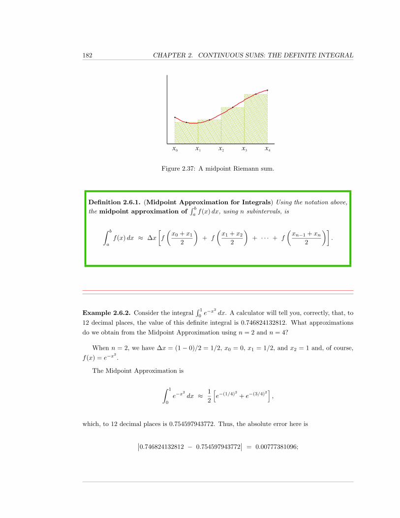
182 CHAPTER 2. CONTINUOUS SUMS: THE DEFINITE INTEGRAL
x0 x1 x2 x3 x4
x0 x1 x2 x3 x4
Figure 2.37: A midpoint Riemann sum.
Definition 2.6.1. (Midpoint Approximation for Integrals) Using the notation above,the midpoint approximation of
∫ baf(x) dx, using n subintervals, is
∫ b
a
f(x) dx ≈ ∆x[f
(x0 + x1
2
)+ f
(x1 + x2
2
)+ · · · + f
(xn−1 + xn
2
)].
Example 2.6.2. Consider the integral∫ 1
0e−x
2dx. A calculator will tell you, correctly, that, to
12 decimal places, the value of this definite integral is 0.746824132812. What approximationsdo we obtain from the Midpoint Approximation using n = 2 and n = 4?
When n = 2, we have ∆x = (1 − 0)/2 = 1/2, x0 = 0, x1 = 1/2, and x2 = 1 and, of course,f(x) = e−x
2.
The Midpoint Approximation is
∫ 1
0
e−x2dx ≈ 1
2
[e−(1/4)2 + e−(3/4)2
],
which, to 12 decimal places is 0.754597943772. Thus, the absolute error here is
∣∣0.746824132812 − 0.754597943772∣∣ = 0.00777381096;
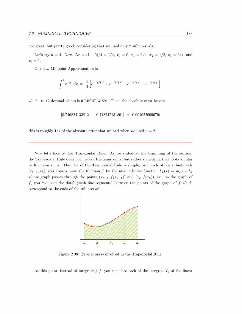
2.6. NUMERICAL TECHNIQUES 183
not great, but pretty good, considering that we used only 2 subintervals.
Let’s try n = 4. Now, ∆x = (1 − 0)/4 = 1/4, x0 = 0, x1 = 1/4, x2 = 1/2, x3 = 3/4, andx4 = 1.
Our new Midpoint Approximation is
∫ 1
0
e−x2dx ≈ 1
4
[e−(1/8)2 + e−(3/8)2 + e−(5/8)2 + e−(7/8)2
],
which, to 12 decimal places is 0.748747131891. Thus, the absolute error here is
∣∣0.746824132812 − 0.748747131891∣∣ = 0.001922999079;
this is roughly 1/4 of the absolute error that we had when we used n = 2.
Now let’s look at the Trapezoidal Rule. As we stated at the beginning of the section,the Trapezoidal Rule does not involve Riemann sums, but rather something that looks similarto Riemann sums. The idea of the Trapezoidal Rule is simple; over each of our subintervals[xk−1, xk], you approximate the function f by the unique linear function Lk(x) = mkx + bk
whose graph passes through the points (xk−1, f(xk−1)) and (xk, f(xk)), i.e., on the graph off , you “connect the dots” (with line segments) between the points of the graph of f whichcorrespond to the ends of the subinterval.
x0 x1 x2 x3 x4
x0 x1 x2 x3 x4Figure 2.38: Typical areas involved in the Trapezoidal Rule.
At this point, instead of integrating f , you calculate each of the integrals Ik of the linear
184 CHAPTER 2. CONTINUOUS SUMS: THE DEFINITE INTEGRAL
functions Lk(x) = mkx + bk over the interval [xk−1, xk], and then you add these integralstogether. What you obtain for Ik is
Ik =∆x2
[f(xk−1) + f(xk)
].
If f is positive, you should recognize this as the area of a trapezoid: one half the “height” (here,it’s the width) times the sum of the lengths of the bases. Adding these together, we find theapproximation ∫ b
a
f(x) dx ≈ I1 + I2 + I3 + · · · + In−1 + In =
∆x2
[f(x0) + f(x1)
]+
∆x2
[f(x1) + f(x2)
]+
∆x2
[f(x2) + f(x3)
]+ · · ·+
∆x2
[f(xn−2) + f(xn−1)
]+
∆x2
[f(xn−1) + f(xn)
].
Factoring out the ∆x2 , and combining the pairs of overlapping terms everywhere, except for at
the f(x0) and f(xn) terms, we obtain the following approximation.
Definition 2.6.3. (Trapezoidal Rule) Using the notation above, the Trapezoidal RuleApproximation of
∫ baf(x) dx, using n subintervals, is
∫ b
a
f(x) dx ≈ ∆x2
[f(x0) + 2f(x1) + 2f(x2) + · · ·+ 2f(xn−1) + f(xn)
].
Note that the pattern of the coefficients for f(xk) in the Trapezoidal Rule is that the firstand last coefficients are 1’s and, aside from that, the coefficients are always 2’s.
Example 2.6.4. As in Example 2.6.2, consider the integral∫ 1
0e−x
2dx. Recall that, to 12
decimal places, the value of this definite integral is 0.746824132812. What approximations dowe obtain from the Trapezoidal Rule using n = 2 and n = 4?
When n = 2, as before, we have ∆x = (1− 0)/2 = 1/2, x0 = 0, x1 = 1/2, and x2 = 1.
2.6. NUMERICAL TECHNIQUES 185
The Trapezoidal Rule Approximation is
∫ 1
0
e−x2dx ≈ 1
4
[e−(0)2 + 2e−(1/2)2 + e−(1)2
],
which, to 12 decimal places is 0.731370251829. Thus, the absolute error here is
∣∣0.746824132812 − 0.731370251829∣∣ = 0.015453880983.
Note that this is roughly double the absolute error that we had when we used the midpointRiemann sum with n = 2.
What about when n = 4? As before, ∆x = (1 − 0)/4 = 1/4, x0 = 0, x1 = 1/4, x2 = 1/2,x3 = 3/4, and x4 = 1.
Our new Trapezoidal Rule Approximation is
∫ 1
0
e−x2dx ≈ 1
8
[e−(0)2 + 2e−(1/4)2 + 2e−(1/2)2 + 2e−(3/4)2 + e−(1)2
],
which, to 12 decimal places is 0.742984097800. Thus, the absolute error here is
∣∣0.746824132812 − 0.742984097800∣∣ = 0.003840035012.
As with the Midpoint Approximation, this new approximation, using the Trapezoidal Rule withn = 4 has roughly 1/4 of the absolute error that we had when we used the Trapezoidal Rulewith n = 2. However, you should also notice that it is still true that the absolute error, withn = 4, using the Trapezoidal Rule, is roughly double the error, with n = 4, using the midpointRiemann sum.
What is Simpson’s Rule? In a sense, Simpson’s Rule is the next step after the TrapezoidalRule. The Trapezoidal Rule takes pairs of successive points on the graph of f , as determined bythe endpoints of the subintervals. Two points determine a line, and so determine a linear functionL = mx+ b. On the k-th subinterval, we approximate f by the linear function Lk = mkx+ bk
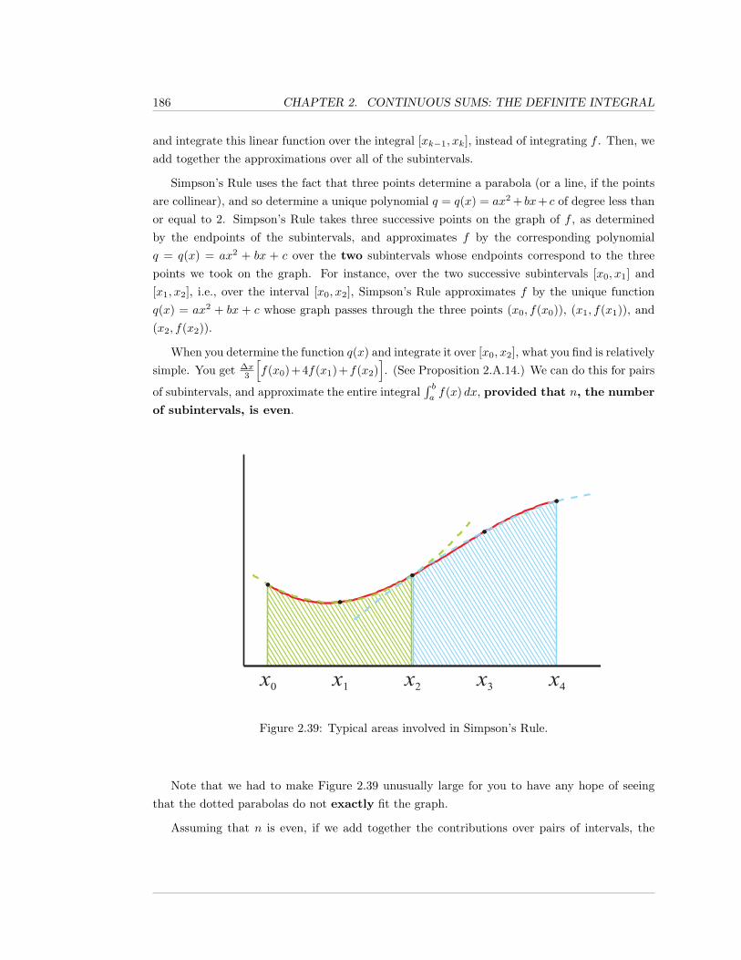
186 CHAPTER 2. CONTINUOUS SUMS: THE DEFINITE INTEGRAL
and integrate this linear function over the integral [xk−1, xk], instead of integrating f . Then, weadd together the approximations over all of the subintervals.
Simpson’s Rule uses the fact that three points determine a parabola (or a line, if the pointsare collinear), and so determine a unique polynomial q = q(x) = ax2 + bx+ c of degree less thanor equal to 2. Simpson’s Rule takes three successive points on the graph of f , as determinedby the endpoints of the subintervals, and approximates f by the corresponding polynomialq = q(x) = ax2 + bx + c over the two subintervals whose endpoints correspond to the threepoints we took on the graph. For instance, over the two successive subintervals [x0, x1] and[x1, x2], i.e., over the interval [x0, x2], Simpson’s Rule approximates f by the unique functionq(x) = ax2 + bx + c whose graph passes through the three points (x0, f(x0)), (x1, f(x1)), and(x2, f(x2)).
When you determine the function q(x) and integrate it over [x0, x2], what you find is relativelysimple. You get ∆x
3
[f(x0)+4f(x1)+f(x2)
]. (See Proposition 2.A.14.) We can do this for pairs
of subintervals, and approximate the entire integral∫ baf(x) dx, provided that n, the number
of subintervals, is even.
x0 x1 x2 x3 x4Figure 2.39: Typical areas involved in Simpson’s Rule.
Note that we had to make Figure 2.39 unusually large for you to have any hope of seeingthat the dotted parabolas do not exactly fit the graph.
Assuming that n is even, if we add together the contributions over pairs of intervals, the
2.6. NUMERICAL TECHNIQUES 187
approximation that we obtain is ∫ b
a
f(x) dx ≈
∆x3
[f(x0) + 4f(x1) + f(x2)
]+
∆x3
[f(x2) + 4f(x3) + f(x4)
]+ · · · +
∆x3
[f(xn−4) + 4f(xn−3) + f(xn−2)
]+
∆x3
[f(xn−2) + 4f(xn−1) + f(xn)
].
Factoring out the ∆x3 , and combining the pairs of overlapping terms everywhere, except for at
the f(x0) and f(xn) terms, we obtain the following approximation.
Definition 2.6.5. (Simpson’s Rule) Using the notation above, the Simpson’s Ruleapproximation of
∫ baf(x) dx, using n subintervals, where n is even, is
∫ b
a
f(x) dx ≈ ∆x3
[f(x0) + 4f(x1) + 2f(x2) + 4f(x3) + 2f(x4) + · · ·+ 4f(xn−1) + f(xn)
].
Note that the pattern of the coefficients for f(xk) in Simpson’s Rule is that the first and lastcoefficients are 1’s and, aside from that, the coefficients alternate 4, 2, 4, 2, etc. The next-to-lastcoefficient will always be a 4, due to the fact that n is even.
Example 2.6.6. As in our previous two examples, consider the integral∫ 1
0e−x
2dx. Recall that,
to 12 decimal places, the value of this definite integral is 0.746824132812. What approximationsdo we obtain from Simpson’s Rule using n = 2 and n = 4?
When n = 2, we still have ∆x = (1− 0)/2 = 1/2, x0 = 0, x1 = 1/2, and x2 = 1.
The Simpson’s Rule Approximation is
∫ 1
0
e−x2dx ≈ 1
6
[e−(0)2 + 4e−(1/2)2 + e−(1)2
],
which, to 12 decimal places is 0.747180428910. Thus, the absolute error here is
∣∣0.746824132812 − 0.747180428910∣∣ = 0.000356296098.
188 CHAPTER 2. CONTINUOUS SUMS: THE DEFINITE INTEGRAL
Wow! This absolute error is roughly 1/20 of the absolute error using n = 2 for the midpointRiemann sum, and is even roughly 1/5 of the absolute error using n = 4 for the midpointRiemann sum (and, remember, the midpoint Riemann sums gave better approximations thanthe Trapezoidal Rule).
Thus, what we see is that the approximation via Simpson’s Rule, even with a smaller nvalue, is significantly more accurate than those obtained from midpoint Riemann sums or theTrapezoidal Rule. This is typical.
Let’s see what happens when n = 4. As before, ∆x = (1 − 0)/4 = 1/4, x0 = 0, x1 = 1/4,x2 = 1/2, x3 = 3/4, and x4 = 1.
Our new Simpson’s Rule Approximation is
∫ 1
0
e−x2dx ≈ 1
12
[e−(0)2 + 4e−(1/4)2 + 2e−(1/2)2 + 4e−(3/4)2 + e−(1)2
],
which, to 12 decimal places is 0.746855379791. Thus, the absolute error here is
∣∣0.746824132812 − 0.746855379791∣∣ = 0.000031246979.
This new approximation, using Simpson’s Rule with n = 4 has roughly 1/10 of the absoluteerror that we had when we used Simpson’s Rule with n = 2.
It is reasonable to ask if it is possible to make precise in what sense midpoint Riemann sums,the Trapezoidal Rule, and Simpson’s Rule are “reasonable” approximation methods. Basically,the question is: what can an instructor say to a student who wants credit for claiming “
∫ 1
0e−x
2dx
is approximately 1, 000, 000, it’s just that the error is really large”?
A possible answer is provided by the following three theorems, which we prove in the Techni-cal Matters section, Section 2.A. These theorems give upper bounds on the absolute error whenapproximating an integral by using midpoint Riemann sums, the Trapezoidal Rule, and/orSimpson’s Rule, provided that the integrand possesses enough derivatives. In particular, thesetheorems imply that, for all three approximation techniques, the error approaches zero as napproaches ∞.
2.6. NUMERICAL TECHNIQUES 189
Theorem 2.6.7. Suppose that a < b and the midpoint Riemann sum with n subintervals ofequal length ∆x is used to approximate
∫ baf(x) dx.
If f ′′(x) exists for all x in some open interval containing the closed interval [a, b] and,if there exists a number M ≥ 0 such that, for all x in [a, b], |f ′′(x)| ≤M , then the absolutevalue of the error, Emdpt, satisfies the inequality
|Emdpt| ≤M(∆x)3n
24=
M(b− a)3
24n2.
Proof. See Theorem 2.A.15.
If, in fact, f ′′ above is continuous on the interval [a, b], then the best, i.e., smallest, valuethat you can use for M above is the maximum value of f ′′ on [a, b].
Theorem 2.6.8. Suppose that a < b and the Trapezoidal Rule with n subintervals of equallength ∆x is used to approximate
∫ baf(x) dx.
If f ′′(x) exists for all x in some open interval containing the closed interval [a, b] and,if there exists a number M ≥ 0 such that, for all x in [a, b], |f ′′(x)| ≤M , then the absolutevalue of the error, Etrap, satisfies the inequality
|Etrap| ≤M(∆x)3n
12=
M(b− a)3
12n2
Proof. See Theorem 2.A.16.
Remark 2.6.9. Note that our upper bound for the absolute value of the error in approximatingwith the Trapezoidal Rule is precisely twice the upper bound that we had for approximatingwith midpoint Riemann sums. This is why references frequently say that midpoint Riemannsums generally provide a better approximation to definite integrals than does the TrapezoidalRule. Understand, however, that the general upper bounds on the absolute values of the errorsthat appear in the theorems don’t have to be very close to the true absolute values of the errors;they are simply gross upper bounds.
190 CHAPTER 2. CONTINUOUS SUMS: THE DEFINITE INTEGRAL
In particular, the absolute value of the error using the Trapezoidal Rule can be strictlysmaller than what you obtain from midpoint Riemann sums. That’s just not what we expect,in general.
Theorem 2.6.10. Suppose that a < b, n is even, and Simpson’s Rule with n subintervalsof equal length ∆x is used to approximate
∫ baf(x) dx.
If f (4)(x) exists for all x in some open interval containing the closed interval [a, b] and,if there exists a number M ≥ 0 such that, for all x in [a, b], |f (4)(x)| ≤M , then the absolutevalue of the error, ESimp, satisfies the inequality
|ESimp| ≤M(∆x)5n
180=
M(b− a)5
180n4.
Proof. See Theorem 2.A.17.
Remark 2.6.11. If f(x) is a quadratic polynomial, then it should not be surprising thatSimpson’s Rule would give the exact value of the integral; after all, Simpson’s Rule is obtainedby approximating the given function with quadratic functions.
What is somewhat surprising is that, even if f(x) is a cubic polynomial, the error boundabove tells us that Simpson’s Rule still yields the exact value of the integral, for the fourthderivative of a cubic polynomial is 0, and so the M in the error statement could be taken to be0.
Let’s look at an example for which we can produce an easy anti-derivative, and can easilyfind bounds on the second and fourth derivatives, so that we can see how two different approx-imations compare with the exact answer. Understand, however, that the true value of theseapproximations is in cases like
∫ 1
0e−x
2dx, where we can’t produce a convenient anti-derivative.
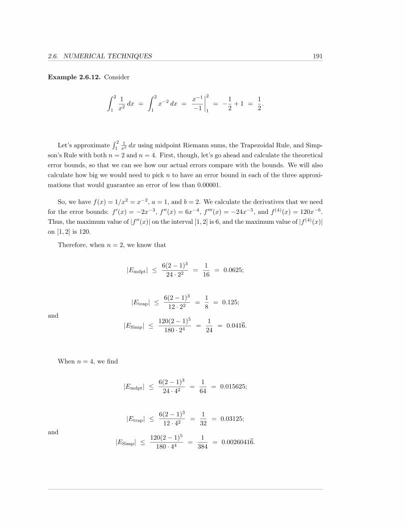
2.6. NUMERICAL TECHNIQUES 191
Example 2.6.12. Consider
∫ 2
1
1x2
dx =∫ 2
1
x−2 dx =x−1
−1
∣∣∣∣21
= −12
+ 1 =12.
Let’s approximate∫ 2
11x2 dx using midpoint Riemann sums, the Trapezoidal Rule, and Simp-
son’s Rule with both n = 2 and n = 4. First, though, let’s go ahead and calculate the theoreticalerror bounds, so that we can see how our actual errors compare with the bounds. We will alsocalculate how big we would need to pick n to have an error bound in each of the three approxi-mations that would guarantee an error of less than 0.00001.
So, we have f(x) = 1/x2 = x−2, a = 1, and b = 2. We calculate the derivatives that we needfor the error bounds: f ′(x) = −2x−3, f ′′(x) = 6x−4, f ′′′(x) = −24x−5, and f (4)(x) = 120x−6.Thus, the maximum value of |f ′′(x)| on the interval [1, 2] is 6, and the maximum value of |f (4)(x)|on [1, 2] is 120.
Therefore, when n = 2, we know that
|Emdpt| ≤6(2− 1)3
24 · 22=
116
= 0.0625;
|Etrap| ≤6(2− 1)3
12 · 22=
18
= 0.125;
and|ESimp| ≤
120(2− 1)5
180 · 24=
124
= 0.0416.
When n = 4, we find
|Emdpt| ≤6(2− 1)3
24 · 42=
164
= 0.015625;
|Etrap| ≤6(2− 1)3
12 · 42=
132
= 0.03125;
and|ESimp| ≤
120(2− 1)5
180 · 44=
1384
= 0.00260416.
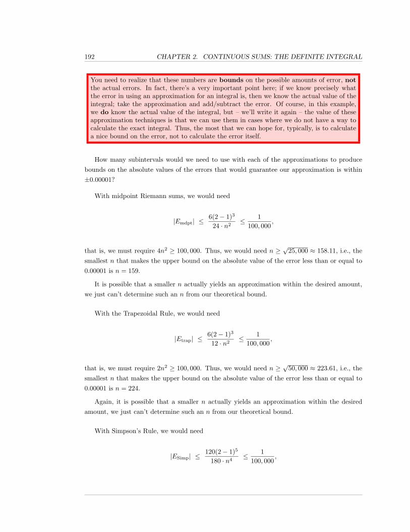
192 CHAPTER 2. CONTINUOUS SUMS: THE DEFINITE INTEGRAL
You need to realize that these numbers are bounds on the possible amounts of error, notthe actual errors. In fact, there’s a very important point here; if we know precisely whatthe error in using an approximation for an integral is, then we know the actual value of theintegral; take the approximation and add/subtract the error. Of course, in this example,we do know the actual value of the integral, but – we’ll write it again – the value of theseapproximation techniques is that we can use them in cases where we do not have a way tocalculate the exact integral. Thus, the most that we can hope for, typically, is to calculatea nice bound on the error, not to calculate the error itself.
How many subintervals would we need to use with each of the approximations to producebounds on the absolute values of the errors that would guarantee our approximation is within±0.00001?
With midpoint Riemann sums, we would need
|Emdpt| ≤6(2− 1)3
24 · n2≤ 1
100, 000,
that is, we must require 4n2 ≥ 100, 000. Thus, we would need n ≥√
25, 000 ≈ 158.11, i.e., thesmallest n that makes the upper bound on the absolute value of the error less than or equal to0.00001 is n = 159.
It is possible that a smaller n actually yields an approximation within the desired amount,we just can’t determine such an n from our theoretical bound.
With the Trapezoidal Rule, we would need
|Etrap| ≤6(2− 1)3
12 · n2≤ 1
100, 000,
that is, we must require 2n2 ≥ 100, 000. Thus, we would need n ≥√
50, 000 ≈ 223.61, i.e., thesmallest n that makes the upper bound on the absolute value of the error less than or equal to0.00001 is n = 224.
Again, it is possible that a smaller n actually yields an approximation within the desiredamount, we just can’t determine such an n from our theoretical bound.
With Simpson’s Rule, we would need
|ESimp| ≤120(2− 1)5
180 · n4≤ 1
100, 000,
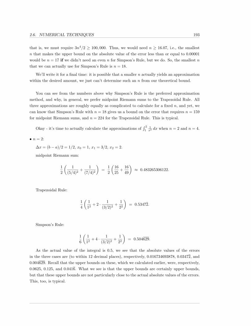
2.6. NUMERICAL TECHNIQUES 193
that is, we must require 3n4/2 ≥ 100, 000. Thus, we would need n ≥ 16.07, i.e., the smallestn that makes the upper bound on the absolute value of the error less than or equal to 0.00001would be n = 17 if we didn’t need an even n for Simpson’s Rule, but we do. So, the smallest nthat we can actually use for Simpson’s Rule is n = 18.
We’ll write it for a final time: it is possible that a smaller n actually yields an approximationwithin the desired amount, we just can’t determine such an n from our theoretical bound.
You can see from the numbers above why Simpson’s Rule is the preferred approximationmethod, and why, in general, we prefer midpoint Riemann sums to the Trapezoidal Rule. Allthree approximations are roughly equally as complicated to calculate for a fixed n, and yet, wecan know that Simpson’s Rule with n = 18 gives us a bound on the error that requires n = 159for midpoint Riemann sums, and n = 224 for the Trapezoidal Rule. This is typical.
Okay - it’s time to actually calculate the approximations of∫ 2
11x2 dx when n = 2 and n = 4.
• n = 2:
∆x = (b− a)/2 = 1/2, x0 = 1, x1 = 3/2, x2 = 2.
midpoint Riemann sum:
12
(1
(5/4)2+
1(7/4)2
)=
12
(1625
+1649
)≈ 0.483265306122.
Trapezoidal Rule:
14
(112
+ 2 · 1(3/2)2
+122
)= 0.53472.
Simpson’s Rule:
16
(112
+ 4 · 1(3/2)2
+122
)= 0.504629.
As the actual value of the integral is 0.5, we see that the absolute values of the errorsin the three cases are (to within 12 decimal places), respectively, 0.016734693878, 0.03472, and0.004629. Recall that the upper bounds on these, which we calculated earlier, were, respectively,0.0625, 0.125, and 0.0416. What we see is that the upper bounds are certainly upper bounds,but that these upper bounds are not particularly close to the actual absolute values of the errors.This, too, is typical.
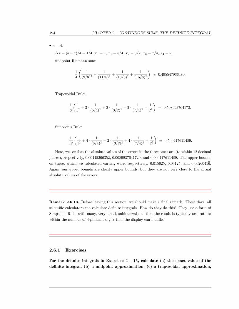
194 CHAPTER 2. CONTINUOUS SUMS: THE DEFINITE INTEGRAL
• n = 4:
∆x = (b− a)/4 = 1/4, x0 = 1, x1 = 5/4, x2 = 3/2, x3 = 7/4, x4 = 2.
midpoint Riemann sum:
14
(1
(9/8)2+
1(11/8)2
+1
(13/8)2+
1(15/8)2
)≈ 0.495547936480.
Trapezoidal Rule:
18
(112
+ 2 · 1(5/4)2
+ 2 · 1(3/2)2
+ 2 · 1(7/4)2
+122
)= 0.508993764172.
Simpson’s Rule:
112
(112
+ 4 · 1(5/4)2
+ 2 · 1(3/2)2
+ 4 · 1(7/4)2
+122
)= 0.500417611489.
Here, we see that the absolute values of the errors in the three cases are (to within 12 decimalplaces), respectively, 0.00445206352, 0.0089937641720, and 0.000417611489. The upper boundson these, which we calculated earlier, were, respectively, 0.015625, 0.03125, and 0.00260416.Again, our upper bounds are clearly upper bounds, but they are not very close to the actualabsolute values of the errors.
Remark 2.6.13. Before leaving this section, we should make a final remark. These days, allscientific calculators can calculate definite integrals. How do they do this? They use a form ofSimpson’s Rule, with many, very small, subintervals, so that the result is typically accurate towithin the number of significant digits that the display can handle.
2.6.1 Exercises
For the definite integrals in Exercises 1 - 15, calculate (a) the exact value of the
definite integral, (b) a midpoint approximation, (c) a trapezoidal approximation,
2.6. NUMERICAL TECHNIQUES 195
and (d) an approximation using Simpson’s Rule. For each of the approximations,
use n = 4. View (a) as an opportunity to practice integration techniques from the
previous chapters.
1.∫ 4
0
5yy − 7
dy.
2.∫ 4
0
√x2 + 16 dx.
3.∫ 10
6
9x− 10x2 − 3x− 10
dx.
4.∫ 4
−4
cosh(4s) ds.
5.∫ 6
2
4t2 + 6t− 2t2 − 1
dt.
6.∫ 12
0
3√x2 + 4
dx.
7.∫ π/6
0
tan(2θ) dθ.
8.∫ 5
1
lnh dh.
9.∫ 6
2
−3z3 + 5z2 + 5z − 5z3 − z2
dz.
10.∫ 6
0
√36− t2 dt.
11.∫ 16
12
24√m2 − 9
dm.
12.∫ 1
0
2du
(144 + u2)2du.
13.∫ 7
3
2p2 + 1p3 + p
dp.
14.∫ 2π
0
sin2 φdφ.
15.∫ 0
−6
√x2 + 12x+ 45 dx.
196 CHAPTER 2. CONTINUOUS SUMS: THE DEFINITE INTEGRAL
16. Prove that the midpoint approximation is in fact equal to∫ b
a
mxdx for arbitrary n. Hint:
show∫ xi+1
ximx+ b dx is equal to the area of the rectangle approximating it.
Determine n, the number of intervals “necessary” to give an approximation of the
definite integral using the specified method with absolute error less than that given.
17.∫ π/4
0
sin(4θ) dθ, Midpoint, Error< 0.001.
18.∫ π/4
0
sin(4θ) dθ, Trapezoid, Error< 0.001.
19.∫ 14238
5134
97x3 − 56πx2 + 42ex− 500 dx, Simpson’s Rule, Error< 0.000001.
Estimate each of the following unpleasant definite integrals using (a) the Midpoint
Rule, (b) the Trapezoidal Rule and (c) Simpson’s Rule.
20.∫ 5
1
ex
xdx, n = 4.
21.∫ π
0
sin(sin t) dt. n = 6.
22.∫ π/2
0
sin(y2) dy. n = 8. Note: this is one of the Fresnel integrals, introduced in the
exercises of the previous chapter.
23.∫ 1
0
dz√z4 + 1
. n = 10.
24.∫ 1/2
0
ln(1 + x)1 + x
dx. n = 6.
25. Use the fact that lnx =∫ x
1
dt
tand the Trapezoidal Rule with n = 10 to approximate ln 2.
26. Redo the previous problem using n = 10 and Simpson’s rule.
27. Use the formulaπ
4=∫ 1
0
dy
1 + y2to estimate π. Use the trapezoid formula with n = 10.
28. Redo the previous problem using n = 10 and Simpson’s rule.
In Exercises 29 - 32, calculate an upper bound for the absolute error of the definite
integral in terms of n when approximated with (a) the Midpoint Method and (b)
the Trapezoidal Rule.
2.6. NUMERICAL TECHNIQUES 197
29.∫ 9
1
dy
y.
30.∫ 2π
0
sin2 t dt.
31.∫ 12
0
ez dz.
32.∫ 1
−1
e−x2dx. Hint: To find the maximum absolute value of the derivatives, note that all
derivatives are of the form p(x)e−x2
where p(x) is a polynomial. It takes some fortitude tofactor these polynomials and correctly apply the first or second derivative tests, but someof the roots are obvious.
33. What is the upper bound on the absolute error of∫ 3
0
ex2dx when estimated with Simp-
son’s Rule? Leave your answer in terms of n. Hint: even though Simpson’s Rule requiresmore derivative taking than the Midpoint Method, this problem is easier than the pre-vious problem since the polynomial appearing in the 4th derivative is easier to analyze.
34. Generalize the previous problem. Let E(n, b) be the upper bound of Simpson’s approx-
imation of∫ b
0
ex2dx when [0, b] is subdivided into n equally spaced intervals. What is
E(n, b)?
35. Prove that if n = 4, the Simpson’s approximation of∫ b
a
x2 dx is exact.
A random variable is said to follow the standard normal distribution if it is normally
distributed with mean zero and standard deviation one (µ = 0, σ = σ2 = 1). Use this
information to solve Exercises 36 - 40.
36. Show that the density function of a standard normal distribution is1√2πe−x
2/2.
37. a. Suppose a data set follows a standard normal distribution. Use the Midpoint Rulewith n = 4 to approximate the proportion of data between 0 and 1.
b. Based on your result in (a), approximately how much of the data falls between −1and 1? Hint: the density function is symmetric about the y-axis.
38. a. Suppose a data set follows a standard normal distribution. Use the Trapezoidal Rulewith n = 4 to approximate the proportion of data between 0 and 2.
b. Based on your result in (a), approximately how much of the data falls between −2
and 2?
198 CHAPTER 2. CONTINUOUS SUMS: THE DEFINITE INTEGRAL
39. Suppose that the mature height of a certain tree species is normally distributed withmean 16 feet and standard deviation of 2 feet. What proportion of trees are between 14and 18 feet tall? Hint: given a normal distribution with parameters µ and σ, make thesubstitution z =
x− µσ
before evaluating. You should be able to use one of the prior twoproblems to help answer this question.
40. Suppose a test is administered to gauge the effect of alcohol on driving ability. A largesample of individuals is given one alcoholic beverage, and their response time to a certainstimulus is measured. Suppose the response time is normally distributed with mean threeseconds and standard deviation 0.6 seconds. What proportion of the individuals’ response
times falls between 1.8 and 4.2 seconds?
Up to this point, we’ve used the various methods in this chapter to approximate
definite integrals of a given continuous, or at least integrable, function. Since these
approximations depend only on knowledge of the function at finitely many points,
they may be adapted to applications where a definite integral is required, but the
integrand is known only at finitely many points.
41. Recall that if the force exerted on an object x meters from the origin is given by f(x), then
the work done in moving the object from a to b meters from the origin is W =∫ b
a
f(x) dx.
Suppose a 3 kilogram mass is being moved from 9 to 17 meters from the origin and theacceleration of the particle is measured every 2 meters in meters per second per second asshown in the table below. Use the Midpoint Method to approximate the total work done.
x Acceleration10 2.512 514 216 -1
42. Suppose that a device is placed in a race car that measure the instantaneous velocity attwo second intervals. The data is shown below. Use Simpson’s Rule to estimate the totaldistance traveled by the car between t = 0 and t = 14 seconds.
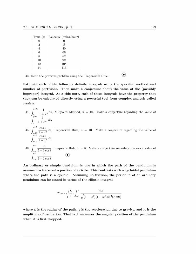
2.6. NUMERICAL TECHNIQUES 199
Time (t) Velocity (miles/hour)0 02 154 406 668 8210 9212 10814 116
43. Redo the previous problem using the Trapezoidal Rule.
Estimate each of the following definite integrals using the specified method and
number of partitions. Then make a conjecture about the value of the (possibly
improper) integral. As a side note, each of these integrals have the property that
they can be calculated directly using a powerful tool from complex analysis called
residues.
44.∫ 100
0
11 + x4
dx, Midpoint Method, n = 10. Make a conjecture regarding the value of∫ ∞0
11 + x4
dx.
45.∫ 10
−10
cos z1 + z2
dz, Trapezoidal Rule, n = 10. Make a conjecture regarding the value of∫ ∞−∞
cos z1 + z2
dz.
46.∫ π
−π
dt
5 + 3 cos t, Simpson’s Rule, n = 8. Make a conjecture regarding the exact value of∫ π
−π
dt
5 + 3 cos t.
An ordinary or simple pendulum is one in which the path of the pendulum is
assumed to trace out a portion of a circle. This contrasts with a cycloidal pendulum
where the path is a cycloid. Assuming no friction, the period T of an ordinary
pendulum can be stated in terms of the elliptic integral
T = 2
√L
g·∫ 1
−1
dw√(1− w2)(1− w2 sin2(A/2))
where L is the radius of the path, g is the acceleration due to gravity, and A is the
amplitude of oscillation. That is A measures the angular position of the pendulum
when it is first dropped.
200 CHAPTER 2. CONTINUOUS SUMS: THE DEFINITE INTEGRAL
47. Suppose A = π/2, g = 9.8 m/sec2 and L = 1 meter. Use Simpson’s Rule with n = 4to estimate the period. As the integral is improper, make your estimation of the interval[−.95, .95].
48. Redo the previous problem with A = π/4.
49. Argue that if the period is small, the period can be approximated by
2
√L
g·∫ 1
−1
dw√1− w2
.
This expression is therefore independent of the amplitude. Evaluate this integral directlyusing L = 1 meter.
50. Is your answer to the previous problem closer to the Simpson’s approximation with A =π/2 or A = π/4? Why does this make sense?
2.A. TECHNICAL MATTERS 201
Appendix 2.A Technical Matters
In this section, we want to describe the technical framework for proving many of the theoremson definite integrals. Still, there are many details beyond the scope of what we want to presenteven in this technical appendix; our primary reference for these details is [4].
Theorem 2.A.1. The limit of Riemann sums, the definite integral, given in Definition 2.3.1 isunique, if it exists.
In addition, if f is Riemann integrable on the interval [a, b],∫ baf(x) dx = L, and
(Pn,Sn) is a sequence of sampled partitions of [a, b] such that limn→∞
|| Pn || = 0, then
limn→∞
RSnPn(f) = L.
Proof. Clearly, proving the sequence statement proves the entire theorem.
Suppose that∫ baf(x) dx exists and equals L, and suppose that (Pn,Sn) is a sequence of
sampled partitions of [a, b] such that limn→∞
|| Pn || = 0.
Let ε > 0. Then, by definition of the Riemann integral, there exists δ > 0 such that, for allpartitions P = {x0, . . . , xn} of [a, b], such that ||P|| < δ, for all sample sets {s1, . . . , sn} for P,
∣∣∣∣∣n∑i=1
f(si)∆xi − L
∣∣∣∣∣ < ε.
As limn→∞
|| Pn || = 0, there exists a positive integer N such that, for all n ≥ N , || Pn || < δ.Hence, for all n ≥ N , if Pn = {x0, . . . , xn} and Sn = {s1, . . . , sn},
∣∣∣∣∣n∑i=1
f(si)∆xi − L
∣∣∣∣∣ < ε,
that is,limn→∞
RSnPn(f) = L.
Before stating any further results, we remark that Theorem 2.3.6 tells us that unboundedfunctions (see Definition 2.3.4) are not Riemann integrable. Consequently, below, we will be
202 CHAPTER 2. CONTINUOUS SUMS: THE DEFINITE INTEGRAL
concerned with the case where f is a bounded function, until we get to the results on improperintegrals.
It is a defining property of the real numbers that every non-empty set of real numbers, whichis bounded above, has a least upper bound or supremum. It follows, by negating, that every non-empty set of real numbers, which is bounded below, has a greatest lower bound or infimum. For abounded set V of real numbers, you should think of the supremum and infimum as the numbersthat “want” to be the maximum and minimum values, respectively, in V , though neither thesupremum or infimum need actually be contained in V .
Now suppose that f is a bounded function (see Definition 2.3.4) on a set E of real numbers.This means that the set V = f(E) = {f(x) | x ∈ E} is bounded, and so possesses a supremumand infimum; we denote these, respectively, by Mf (E) and mf (E).
The Extreme Value Theorem, (see [2] or [4]), tells us that a continuous function f on a closedinterval [a, b] is bounded and that, in fact, Mf ([a, b]) and mf ([a, b]) are in the set f([a, b]), sothat they are, respectively, the maximum and minimum values of f on [a, b].
Now, suppose that f is bounded on the closed interval [a, b], and that P = (x0, . . . , xn)is a partition of [a, b]. We would like to pick sample points which maximize or minimize theRiemann sums, but such sample points need not exist (though they would if f were continuous).However, we can “fake” it by using the supremum and infimum of f on each subinterval of thepartition. Thus, we define the upper and lower sums Uf (P) and Lf (P), respectively, of f withrespect to the partition P to be
Uf (P) =n∑i=1
Mf ([xi−1, xi]) ∆xi,
and
Lf (P) =n∑i=1
mf ([xi−1, xi]) ∆xi.
It follows immediately that Uf (P) is the least upper bound of all of the Riemann sums of f ,using the partition P, and that Lf (P) is the greatest lower bound of all of the Riemann sumsof f , using the partition P.
Note that it is immediate that, if a partition P∗ is a refinement of a partition P, then
Uf (P∗)− Lf (P∗) ≤ Uf (P)− Lf (P).
2.A. TECHNICAL MATTERS 203
The fundamental integrability result that we need, for bounded functions, is the following,which we state without proof; see Theorem 3.2.7 of [4].
Theorem 2.A.2. Suppose that f is bounded on the interval [a, b]. Then, f is Riemann integrableon [a, b] if and only if, for all ε > 0, there exists a partition P of [a, b] such that
Uf (P)− Lf (P) < ε.
Given Theorem 2.A.2, the integrability of continuous functions follows almost immediatelyfrom a basic fact: continuous functions on closed bounded intervals [a, b] are uniformly contin-uous. That is:
Theorem 2.A.3. If f is continuous on the closed interval [a, b], then, for all ε > 0, there existsδ > 0 such that, if x1 and x2 are in [a, b] and |x1 − x2| < δ, then f(x1)− f(x2) < ε.
Proof. See Theorem 2.2.12 of [4].
The “uniform” in “uniformly continuous” refers to the fact that, for a given ε > 0, there is auniform δ > 0 that works everywhere in the interval; normal continuity allows δ to vary as youchange one of the points.
It is now easy to prove:
Theorem 2.A.4. Suppose that f is continuous on the interval [a, b], where a < b. Then, f isRiemann integrable on [a, b].
Proof. Let ε > 0. Then, ε/(b− a) > 0, and so, by Theorem 2.A.3, there exists δ > 0 such that,if x1 and x2 are in [a, b] and |x1 − x2| < δ, then |f(x1)− f(x2)| < ε/(b− a).
Let P = (x0, . . . , xn) be a partition of [a, b] with mesh < δ. We claim that Uf (P)−Lf (P) < ε,which would prove that f is Riemann integrable by Theorem 2.A.2.
As || P || < δ, for any two points ai and bi in the subinterval [xi−1, xi], |ai − bi| < δ. Byconsidering the points in the subinterval where f attains its maximum and minimum values, weconclude that Mf ([xi−1, xi])−mf ([xi−1, xi]) < ε/(b− a) and, hence, that
n∑i=1
(Mf ([xi−1, xi])−mf ([xi−1, xi])
)∆xi <
n∑i=1
ε
b− a∆xi =
ε
b− a
n∑i=1
∆xi = ε,
204 CHAPTER 2. CONTINUOUS SUMS: THE DEFINITE INTEGRAL
i.e., that
Uf (P)− Lf (P) < ε.
We can now prove Theorem 2.3.8.
Theorem 2.A.5. Bounded, piecewise-continuous functions on closed intervals are Riemannintegrable.
Proof. By dividing the interval [a, b] into subintervals such that each subinterval has a discon-tinuity at, at most, one endpoint. By Theorem 2.3.16, it is enough for us to prove that f isRiemann integrable on such subintervals. Thus, we will assume that f is bounded on [a, b], with|f(x)| ≤ B, for x in [a, b], and has a single discontinuity at a. Note that, if B = 0, f is identically0 on [a, b], and we’re finished; so assume that B > 0.
Now, let ε > 0. Consider first the partition of [a, b] given by P = (a, a + ε/(4B), b). As fis continuous on [a + ε/(4B), b], f is integrable on this subinterval, and so, by Theorem 2.A.2,there exists a partition P = (x0, . . . , xn) of [a+ ε/(4B), b] such that Uf (P)− Lf (P) < ε/2. LetP∗ be the partition of [a, b] given by (a, x0, . . . , xn).
Then, from the definitions, it follows at once that
Uf (P∗) = Mf ([a, x0]) · ε/(4B) + Uf (P)
and
Lf (P∗) = mf ([a, x0]) · ε/(4B) + Lf (P).
Also, note that Mf ([a, x0]) ≤ B, while mf ([a, x0]) ≥ −B, so that −mf ([a, x0]) ≤ B, andMf ([a, x0])−mf ([a, x0]) ≤ 2B.
Therefore,
Uf (P∗) − Lf (P∗) = Mf ([a, x0]) · ε/(4B) + Uf (P) − mf ([a, x0]) · ε/(4B) − Lf (P) =
(Mf ([a, x0]) − mf ([a, x0])
)· ε
4B+[Uf (P) − Lf (P)
]<
ε
2+
ε
2= ε,
and we are finished by Theorem 2.A.2.
Theorem 2.A.6. Suppose that a < b.
2.A. TECHNICAL MATTERS 205
1. If f is Riemann integrable on [a, b] and a ≤ c < d ≤ b, then f is Riemann integrableon [c, d], i.e., if f is Riemann integrable on a given closed interval, then f is Riemannintegrable on any closed subinterval of the given interval.
2. Suppose that a < c < b. Then, f is Riemann integrable on [a, b] if and only if f is Riemannintegrable on [a, c] and [c, b] and, when these equivalent conditions hold,
∫ b
a
f(x) dx =∫ c
a
f(x) dx +∫ b
c
f(x) dx.
Proof. Suppose that f is Riemann integrable on [a, b] and a ≤ c < d ≤ b. By Theorem 2.3.6, fmust be bounded on [a, b] and, hence, is bounded on [c, d].
Let ε > 0. By Theorem 2.A.2, there exists a partition P of [a, b] such that Uf (P)−Lf (P) < ε.Now, let P∗ be the partition of [c, d] formed from the points in [c, d]∩P, together with c and d.Then,
Uf (P∗)− Lf (P∗) ≤ Uf (P)− Lf (P) < ε,
and so, by Theorem 2.A.2, f is integrable on [c, d].
Suppose now that a < c < b.
If f is Riemann integrable on [a, b], then part (1) tells us that f is Riemann integrable on[a, c] and [c, b].
Suppose that f is Riemann integrable on [a, c] and [c, b]. Then, f must be bounded on [a, c]and [c, b] and, hence, on [a, b]. Let ε > 0. Then, ε/2 > 0. By Theorem 2.A.2, there existpartitions P1 and P2 of [a, c] and [c, b], respectively, such that Uf (P1) − Lf (P1) < ε/2 andUf (P2)− Lf (P2) < ε/2. Then, the partition P∗ = P1 ∪ P2 of [a, b] is such that
Uf (P∗)− Lf (P∗) <ε
2+
ε
2= ε.
Therefore, by Theorem 2.A.2, f is Riemann integrable on [a, b].
Now, suppose that f is Riemann integrable on [a, c] and [c, b] and, hence, by the above,Riemann integrable on [a, b]. Let L1 =
∫ caf(x) dx, L2 =
∫ bcf(x) dx, and L =
∫ baf(x) dx. For
each integer n ≥ 1, let P1n and P2
n be partitions of [a, c] and [c, b], respectively, with mesh < 1/n.Let S1
n and S2n be sample sets for the partitions P1
n and P2n, respectively. Let Pn = P1
n ∪ P2n
and Sn = S1n ∪ S2
n. Then, Pn is a partition of [a, b] of mesh < 1/n, and Sn is a sample set forPn (possibly using the sample point c as a sample point for two different subintervals).
206 CHAPTER 2. CONTINUOUS SUMS: THE DEFINITE INTEGRAL
Using Theorem 2.3.3 three times, we find
L1 + L2 = limn→∞
RS1n
P1n(f) + lim
n→∞RS
2n
P2n(f) = lim
n→∞RSnPn(f) = L.
Theorem 2.A.7. (Linearity of Integration) Definite integration over a closed interval is alinear operation, i.e., if f and g are Riemann integrable on [a, b], then, for all constants r ands, the function rf + sg is Riemann integrable on [a, b], and
∫ b
a
(rf(x) + sg(x)
)dx = r
∫ b
a
f(x) dx + s
∫ b
a
g(x) dx.
Proof. Suppose that f and g are Riemann integrable on [a, b]. We will prove that f + g isRiemann integrable on [a, b] and that
∫ b
a
(f(x) + g(x)
)dx =
∫ b
a
f(x) dx +∫ b
a
g(x) dx.
That constants can be pulled out of integrals is left to you in Exercise 52.
Let [c, d] be any closed subinterval of [a, b]. It is trivial to see that
Mf+g([c, d]) ≤ Mf ([c, d]) +Mg([c, d])
and
mf ([c, d]) +mg([c, d]) ≤ mf+g([c, d]).
Therefore, for any partition P of [a, b], Uf+g(P) ≤ Uf (P) + Ug(P) and Lf (P) + Lg(P) ≤Lf+g(P); hence,
Uf+g(P) − Lf+g(P) ≤ [Uf (P) − Lf (P)] + [Ug(P) − Lg(P)] .
It follows immediately from Theorem 2.A.2 that f + g is integrable on [a, b].
Now, let Pn be a partition of [a, b] of mesh < 1/n, and Sn be a sample set for Pn. Using
2.A. TECHNICAL MATTERS 207
Theorem 2.3.3 three times, we find
∫ b
a
(f(x) + g(x)
)dx = lim
n→∞RSnPn(f + g) = lim
n→∞RSnPn(f) + lim
n→∞RSnPn(g) =
∫ b
a
f(x) dx +∫ b
a
g(x) dx.
Using Theorem 2.3.19 (see Theorem 3.3.1 of [4]), it is easy to conclude Theorem 2.3.14.
Theorem 2.A.8. Suppose that f and g are defined on a closed interval [a, b], and that, exceptpossibly for a finite set points in [a, b], f and g are equal at each point in [a, b].
Then, f is Riemann integrable on [a, b] if and only if g is, and when f and g are Riemannintegrable, ∫ b
a
f(x) dx =∫ b
a
g(x) dx.
Proof. As f and g differ on at most a finite number of points, f is bounded if and only if g isbounded. If both functions are unbounded, then Theorem 2.3.6 tells us that both functions arenot Riemann integrable.
Now, suppose that f and g are both bounded, and that f is Riemann integrable. Then, g−fis bounded, and is equal to 0 except at, possibly, a finite number of points, r1, . . . , rp. We claimthat
∫ ba
(g − f)(x) dx = 0; if we show this, we are finished by Theorem 2.3.19, since we wouldthen have ∫ b
a
f(x) dx =∫ b
a
f(x) dx +∫ b
a
(g − f)(x) dx =∫ b
a
g(x) dx.
Let M be the maximum of |(g − f)(ri)| for 1 ≤ i ≤ p. Let P = (x0, . . . , xn) be a partitionof the interval [a, b], and let S = (s1, . . . , sn) be a set of sample points for P.
Then, ∣∣∣∣∣n∑i=1
(g − f)(si)∆xi
∣∣∣∣∣ ≤n∑i=1
|(g − f)(si)| · |∆xi| ≤ M · || P ||,
and, hence,
lim|| P ||→0
RSP(g − f) = 0.
Theorem 2.A.9.
208 CHAPTER 2. CONTINUOUS SUMS: THE DEFINITE INTEGRAL
Theorem 2.A.10. (Fundamental Theorem of Calculus, Part 1) Suppose that f is Rie-mann integrable on [a, b] and is continuous at a point x0 in (a, b). Then, the integral functionI
[a,b]f of f on [a, b] is differentiable at x0 and
(I
[a,b]f
)′(x0) = f(x0).
Thus, if f is continuous on [a, b], then I[a,b]f is an anti-derivative of f on [a, b].
Proof. From the definition of the derivative, we have
(I
[a,b]f
)′(x0) = limx→x0
I[a,b]f (x)− I [a,b]
f (x0)x− x0
= limx→x0
∫ xaf(t) dt −
∫ x0
af(t) dt
x− x0=
limx→x0
∫ xx0f(t) dt
x− x0.
We must show that this limit equals f(x0). We shall show that the limit from the right equalsf(x0), and leave the nearly identical argument from the left as an exercise.
Let ε > 0. By the definition of f being continuous at x0, there exists δ > 0 such that, for allx such that |x− x0| < δ, |f(x)− f(x0)| < ε. We claim that, if 0 < x− x0 < δ, then
∣∣∣∣∣∫ xx0f(t) dt
x− x0− f(x0)
∣∣∣∣∣ < ε, (2.4)
which is what it means that limx→x+0
R xx0f(t) dt
x−x0= f(x0).
To prove the claim in Formula 2.4, fix an x such that 0 < x − x0 < δ. Then, for all t in[x0, x], we have 0 ≤ t− x0 ≤ x− x0 < δ, and so, |t− x0| < δ. Using the defining property of δagain, we conclude that, for all t in [x0, x], |f(t)− f(x0)| < ε.
Therefore, for all t in [x0, x],
f(x0)− ε ≤ f(t) ≤ f(x0) + ε.
2.A. TECHNICAL MATTERS 209
By the monotonicity of integration, Theorem 2.3.20, and Proposition 2.3.12, we conclude that
(f(x0)− ε)(x− x0) =∫ x
x0
(f(x0)− ε) dt ≤∫ x
x0
f(t) dt ≤∫ x
x0
(f(x0) + ε) dt = (f(x0) + ε)(x− x0).
Hence,
f(x0)− ε ≤∫ xx0f(t) dt
x− x0≤ f(x0) + ε,
i.e., ∣∣∣∣∣∫ xx0f(t) dt
x− x0− f(x0)
∣∣∣∣∣ < ε,
as we claimed in Formula 2.4.
The final conclusion of the theorem follows from the first one, together with the continuityof I [a,b]
f , which follows from Theorem 2.4.3.
Theorem 2.A.11. The integral defined in Definition 2.5.11 is independent of the splitting intosubintervals (of the type described in the definition).
Proof. We will prove a lemma, from which the theorem follows immediately.
Suppose that f is continuous on the interval I = [a, b). Let c be such that a < c < b. Weclaim that
∫ baf(x) dx exists if and only if
∫ bcf(x) dx exists and, in this case,
∫ b
a
f(x) dx =∫ c
a
f(x) dx +∫ b
c
f(x) dx.
This is easy:
∫ b
a
f(x) dx = limd→b−
∫ d
a
f(x) dx = limd→b−
[∫ c
a
f(x) dx +∫ d
c
f(x) dx
]=
∫ c
a
f(x) dx + limd→b−
[∫ d
c
f(x) dx
]=∫ c
a
f(x) dx +∫ b
c
f(x) dx.
210 CHAPTER 2. CONTINUOUS SUMS: THE DEFINITE INTEGRAL
Theorem 2.A.12. Let I be an interval of the form [a, b) or (a, b], where we allow the intervals[a,∞) or (−∞, b]. Suppose that, for all x in I, f(x) ≥ 0, and that, for all closed intervals [c, d]contained in I, f is Riemann integrable on [c, d].
Then, if there exists a real number M (an upper bound) such that, for all [c, d] containedin I,
∫ dcf(x) dx ≤M , then
∫ baf(x) dx converges, and what it converges to is less than, or equal
to, M ; in other words, if there is an upper bound M on all of the∫ dcf(x) dx, then
∫ baf(x) dx
converges to the least such upper bound.
In particular, if∫ baf(x) dx diverges, what it diverges to is ∞.
Proof. We will deal with the case where I = [a, b); the other cases are entirely analogous.
For a ≤ d < b, define the function F (d) =∫ daf(x) dx, which exists by assumption. As f ≥ 0,
F is an increasing function on the interval I.
If F gets unboundedly large, then, since F is increasing, limd→b− F (d) =∞. If F is boundedabove by M , then, as F is increasing, F converges to the least upper bound of the set F (I),which is ≤M .
Lemma 2.A.13. Let q(x) = c0 + c1x+ c2x2 + c3x
3, where ci denotes a constant. Then,
∫ h
−hq(x) dx =
h
3
(6c0 + 2c2h2
)=
h
3
(q(−h) + 4q(0) + q(h)
).
Proof. This is a trivial calculation, which we leave to the reader.
Proposition 2.A.14. Let q(x) = ax2 +bx+c. Fix x0. Let h > 0. Let x1 = x0 +h, x2 = x1 +h,and yi = q(xi), for i = 1, 2, 3. Then,
∫ x2
x0
q(x) dx =h
3
(y0 + 4y1 + y2
).
Proof. One can make the substitution u = x− (x0 + h) into the integral and reduce oneself tothe case in Lemma 2.A.13, or do a messy, but simple, algebra problem. One has to show that
[a(x0 + 2h)3
3+b(x0 + 2h)2
2+ c(x0 + 2h)
]−[ax3
0
3+bx2
0
2+ cx0
]=
2.A. TECHNICAL MATTERS 211
h
3
{[ax2
0 + bx0 + c]
+ 4[a(x0 + h)2 + b(x0 + h) + c
]+[a(x0 + 2h)2 + b(x0 + 2h) + c
]}.
We leave either verification as an exercise.
In the proofs below, for notational convenience, we apply the inequalities above in the casewhere a = 0; the general case follows at once by making the substitution u = x− a.
Theorem 2.A.15. Suppose that a < b and the midpoint Riemann sum with n subintervals ofequal length ∆x is used to approximate
∫ baf(x) dx.
If f ′′(x) exists for all x in some open interval containing the closed interval [a, b] and, ifthere exists a number M ≥ 0 such that, for all x in [a, b], |f ′′(x)| ≤M , then the absolute valueof the error, Emdpt, satisfies the inequality
|Emdpt| ≤M(∆x)3n
24=
M(b− a)3
24n2
Proof. We shall prove this for one subinterval, centered at 0. The general result follows byre-centering the intervals, via substitution, and then adding, which leads to the multiplicationby n in the inequality. Let h = ∆x/2.
We will show that ∣∣∣∣∣∫ h
−hf(x) dx − 2hf(0)
∣∣∣∣∣ ≤ Mh3
3.
We must look ahead to the Taylor-Lagrange Theorem, Theorem 4.3.3,, which immediatelyimplies that: if f is twice-differentiable on an open interval I around a point a, and M > 0 is aconstant such that, for all x in I, |f(x)| ≤M , then, for all x in I,
∣∣f(x) −(f(a) + f ′(a)(x− a)
)∣∣ ≤ M
2(x− a)2; (2.5)
Now the proof is easy.
∣∣∣∣∣∫ h
−hf(x) dx − 2hf(0)
∣∣∣∣∣ =
∣∣∣∣∣∫ h
−hf(x) dx −
∫ h
−h
(f(0) + f ′(0)x
)dx
∣∣∣∣∣ ≤∫ h
−h
∣∣f(x) − f(0) − f ′(0)x∣∣ dx ≤ ∫ h
−h
M
2x2 dx =
Mh3
3.
212 CHAPTER 2. CONTINUOUS SUMS: THE DEFINITE INTEGRAL
Theorem 2.A.16. Suppose that a < b and the Trapezoidal Rule with n subintervals of equallength ∆x is used to approximate
∫ baf(x) dx.
If f ′′(x) exists for all x in some open interval containing the closed interval [a, b] and, ifthere exists a number M ≥ 0 such that, for all x in [a, b], |f ′′(x)| ≤M , then the absolute valueof the error, Etrap, satisfies the inequality
|Etrap| ≤M(∆x)3n
12=
M(b− a)3
12n2
Proof. We shall prove this for one subinterval, centered at 0. The general result follows byre-centering the intervals, via substitution, and then adding, which leads to the multiplicationby n in the inequality. Let h = ∆x/2.
We will show that
∣∣∣∣∣∫ h
−hf(x) dx − 2h · f(h) + f(−h)
2
∣∣∣∣∣ ≤ 2Mh3
3.
We integrate by parts twice.
∫ h
−hf(x) dx = xf(x)
∣∣∣h−h−∫ h
−hxf ′(x) dx = hf(h) + hf(−h) −
∫ h
−hxf ′(x) dx =
h(f(h) + f(−h)
)−
[12x2f ′(x)
∣∣∣h−h− 1
2
∫ h
−hx2f ′′(x) dx
].
Therefore,
∣∣∣∣∣∫ h
−hf(x) dx − 2h · f(h) + f(−h)
2
∣∣∣∣∣ =12
∣∣∣∣∣h2f ′(h)− h2f ′(−h)−∫ h
−hx2f ′′(x) dx
∣∣∣∣∣ =
12
∣∣∣∣∣∫ h
−h(h2 − x2)f ′′(x) dx
∣∣∣∣∣ ≤ 12
∫ h
−h(h2 − x2)M dx =
M
2· 4h3
3=
2Mh3
3.
2.A. TECHNICAL MATTERS 213
Theorem 2.A.17. Suppose that a < b, n is even, and Simpson’s Rule with n subintervals ofequal length ∆x is used to approximate
∫ baf(x) dx.
If f (4)(x) exists for all x in some open interval containing the closed interval [a, b] and,if there exists a number M ≥ 0 such that, for all x in [a, b], |f (4)(x)| ≤ M , then the absolutevalue of the error, ESimp, satisfies the inequality
|ESimp| ≤M(∆x)5n
180=
M(b− a)5
180n4.
Proof. We shall prove this for two subintervals, centered at 0. The general result follows byre-centering the intervals, via substitution, and then adding, which leads to the multiplicationby n/2 in the inequality. Let h = ∆x.
Let
ψ(t) =∫ t
−tf(x) dx − t
3
[f(−t) + 4f(0) + f(t)
].
We will show that there exists a c such that −h < c < h and
ψ(h) = −h5f (4)(c)
90.
Let
φ(t) = ψ(t) −(t
h
)5
ψ(t).
One easily calculates that φ(0) = φ′(0) = φ′′(0) = 0 and, for t 6= 0,
φ′′′(t) = −2t2
3
(f ′′′(t)− f ′′′(−t)
2t+
90h5
ψ(h)).
Now, φ(h) = 0, and so, by Rolle’s Theorem, there exists c1 such that 0 < c1 < h andφ′(c1) = 0. Applying Rolle’s Theorem again, we find that there exists c2 such that 0 < c2 <
c1 < h and φ′′(c2) = 0. Applying Rolle’s Theorem yet again, we find that there exists c3 suchthat 0 < c3 < c2 < c1 < h and
φ′′′(c3) = 0.
214 CHAPTER 2. CONTINUOUS SUMS: THE DEFINITE INTEGRAL
Applying the Mean Value Theorem, we conclude that there exists c such that −c3 < c < c3 and
f ′′′(c3) − f ′′′(−c3) = 2c3f (4)(c).
Combining the previous 3 displayed formulas, we conclude that
f (4)(c) +90h5
ψ(h) = 0,
i.e.,
ψ(h) = −h5f (4)(c)
90,
which is what we wanted to show.
Chapter 3
Applications of Integration
In this chapter, we will apply our results on anti-differentiation, definite integrals, and theFundamental Theorem of Calculus to a wide variety of problems involving displacement, distancetraveled, area in the plane, volume, surface areas, mass, centers of mass, rotational inertia, work,and hydrostatic pressure.
Throughout this chapter, we state many of our general results as Propositions, though, inmany cases, these Propositions could be used as Definitions. For instance, we will see the definiteintegral of speed, with respect to time, yields the total distance traveled. We assume that youhave a preconceived notion of the distance traveled, and then conclude that that distance canbe calculated by integrating speed. However, we could, instead, define the distance traveled bythe integral of the speed. Mathematically, this latter approach is more rigorous; it is, however,somewhat intuitively unsatisfying.
Thus, throughout this chapter, we shall usually assume that we have predefined physicalterms, such as distance traveled, volume, mass, etc., and state our integration formulas for thesequantities as Propositions.
We should remark that many of the “applications” in this chapter are actually “pre-applications”,or what some people refer to as “toy problems”. A pre-application or toy problem is a problemthat is stripped of many physical complications or is not inherently of interest in and of itself,but rather is designed mainly to provide some basic example of a fundamental idea that willserve as a building block to tackling more-difficult actual applications.
215
216 CHAPTER 3. APPLICATIONS OF INTEGRATION
3.1 Displacement and Distance Traveledin a Straight Line
In this section, we will apply the definite integral and the Fundamental Theorem of Calculusto problems involving the net change in position, the displacement, of an object, and the totaldistance traveled by the object. If the object changes its direction, these two quantities will not
be the same; the total distance traveled would be greater, while the displacement could, in fact,turn out to be zero if the object ends up back where it started.
The second part of the Fundamental Theorem of Calculus, Theorem 2.4.10, tells us that, ifF is an anti-derivative of a continuous function f on the interval [a, b], then
∫ b
a
f(t) dt = F (t)∣∣∣ba
= F (b)− F (a).
This means that, if we start with a function g(t), which is differentiable on an open intervalcontaining [a, b], and g′(t) is continuous, then
∫ b
a
g′(t) dt =∫ b
a
dg
dtdt = g(b)− g(a).
Suppose now that we have an object moving in a straight line, on which we’ve chosen positiveand negative directions, i.e., suppose that we have an object moving along a coordinate. Letp(t) denote the position (i.e., the coordinate value) of the object at time t.
Assuming that p is continuously differentiable, we know that the velocity v = v(t) of theobject is the rate of change of the position, with respect to time, dp/dt, and the FundamentalTheorem tells us that ∫ b
a
v(t) dt = p(b)− p(a).
The quantity on the right above is the change in the position of the object between timest = a and t = b; recall that this is called the displacement of the object between times a and b.
Of course, when we refer to the velocity function v = v(t), we are implicitly assuming thatthe position function is differentiable, for, otherwise, “the velocity” has no good meaning. Thus,
3.1. DISPLACEMENT AND DISTANCE TRAVELED 217
we can summarize our discussion above by:
Proposition 3.1.1. If the velocity v = v(t), as a function of time t, of an object on acoordinate axis is continuous on the interval [a, b], then the displacement of the objectbetween times t = a and t = b is given by
∫ b
a
v(t) dt.
Example 3.1.2. A particle is moving in a straight line in such a way that its velocity v = v(t),in m/s, at time t seconds, is given by
v = 3t2 − 12t+ 8.
What is the displacement of the particle between times 1 and 3 seconds? Between times 2and 4 seconds? What is the displacement between times 1 and t seconds, for arbitrary t?
Solution:
To answer the first two questions, we need to calculate
∫ 3
1
(3t2 − 12t+ 8) dt and∫ 4
2
(3t2 − 12t+ 8) dt.
We want to apply the Fundamental Theorem, and so we need to find the (or, an) anti-derivative
∫(3t2 − 12t+ 8) dt = 3 · t
3
3− 12 · t
2
2+ 8t+ C = t3 − 6t2 + 8t+ C = t(t− 2)(t− 4) + C.
Therefore, the displacement between times 1 and 3 seconds is
∫ 3
1
(3t2 − 12t+ 8) dt = t(t− 2)(t− 4)∣∣∣31
= −3− 3 = −6 meters;
218 CHAPTER 3. APPLICATIONS OF INTEGRATION
this means that the particle ended up, at time 3 seconds, 6 meters in the negative direction fromwhere it started at time 1 second.
Note that we do not know where the particle is at times 1 and 3 seconds, i.e., we don’t knowthe position function p(t). However, except for the arbitrary constant +C above, we knowp(t), and that’s enough to determine the change in the position.
The displacement of the particle between times 2 and 4 seconds is
∫ 4
2
(3t2 − 12t+ 8) dt = t(t− 2)(t− 4)∣∣∣42
= 0− 0 = 0 meters.
This does not mean that the particle did not move between times 2 and 4 seconds; it merelymeans that the particle, at time 4 seconds, ended up at the same place where the particle wasat time 2 seconds. Of course, this means that the particle had to turn around at some point.Do not confuse displacement, the net change in position, with the total distance traveled.The displacement here, between times 2 and 4 seconds is 0. We shall calculate the total distancetraveled by this particle, between times 2 and 4 seconds, in the next example.
Finally, in this example, we were asked to find the displacement of the particle between times1 and t. This is easy, except that it would now be bad form to use t for the integration variable.You should use essentially any other variable for the dummy variable of integration; the onlyvariables you should avoid are t and v, and maybe d would look confusing too. We’ll use z forthe integration variable. Then, we quickly find that the displacement between times 1 and t
seconds is
∫ t
1
(3z2−12z+8) dz = z(z−2)(z−4)∣∣∣t1
= t(t−2)(t−4)−(1)(−1)(−3) = t3−6t2 +8t−3 meters.
In the example above, we ran into the issue of the distinction between displacement and totaldistance traveled. This distinction arises because, if the velocity v of an object is continuous andalways positive on an interval of time [a, b], then the distance traveled by the object betweentimes a and b is the same as the displacement, namely
∫ bav dt. On the other hand, if the
velocity v of an object is continuous and always negative on an interval of time [a, b], then thedisplacement will be negative; it will be the negation of the distance traveled by the objectbetween times a and b, i.e., the distance traveled will be −
∫ bav dt =
∫ ba−v dt.
Thus, to find the distance traveled, we want to integrate v on intervals where v is positive,
3.1. DISPLACEMENT AND DISTANCE TRAVELED 219
and we want to integrate −v on intervals where v is negative. The way to write this in oneformula is to say that we want to integrate the absolute value |v| in all cases.
Proposition 3.1.3. If the velocity v = v(t), as a function of time t, of an object on acoordinate axis is continuous on the interval [a, b], then the (total) distance traveled bythe object between times t = a and t = b is given by
∫ b
a
|v(t)| dt.
Remark 3.1.4. Proposition 3.1.3 tells us, in a new way, something that we already knew. Ittells us that the total distance traveled, r = r(t), by an object, between some initial time t0 andsome arbitrary time t, is given by
r(t) =∫ t
t0
|v(z)| dz,
where we once again have used z as a new dummy variable, and we’re assuming that v iscontinuous.
Now, the first part of the Fundamental Theorem, Theorem 2.4.7, tells us that
dr
dt= |v(t)|,
i.e., that the (instantaneous) speed of an object can either be defined as the absolute value of thevelocity or as the instantaneous rate of change of the distance traveled, with respect to time.
220 CHAPTER 3. APPLICATIONS OF INTEGRATION
However, it is important to remember that average speed need not be the absolute valueof the average velocity. For instance, an object that returns to where it started, after someamount of time, will have zero displacement and, hence, zero average velocity, but not zeroaverage speed. Average speed is the average rate of change of the distance traveled, withrespect to time. Thus, it is probably best, in the average and/or instantaneous setting,to define speed as the rate of change of the distance traveled, with respect to time, andthen take it as a theorem that the instantaneous speed is equal to the absolute value of theinstantaneous velocity.
Let’s look at an example of calculating the (total) distance traveled.
Example 3.1.5. In Example 3.1.2, we had a particle moving in a straight line in such a waythat its velocity v = v(t), in m/s, at time t seconds, was given by
v = 3t2 − 12t+ 8.
We found that the displacement of the particle between times 2 and 4 seconds is
∫ 4
2
(3t2 − 12t+ 8) dt = t(t− 2)(t− 4)∣∣∣42
= 0− 0 = 0 meters.
Now we’ll ask a different question.
What was the distance traveled by the particle between 2 and 4 seconds?
Solution:
It’s certainly easy to write the appropriate integral. The distance traveled by the particlebetween 2 and 4 seconds was
∫ 4
2
∣∣3t2 − 12t+ 8∣∣ dt meters,
but how do we calculate the integral of the absolute value?
One thing that you definitely don’t do is find an anti-derivative of 3t2 − 12t+ 8, and thentake its absolute value, in hope of producing an anti-derivative of
∣∣3t2−12t+8∣∣. This would
be completely wrong.
3.1. DISPLACEMENT AND DISTANCE TRAVELED 221
There’s really only one thing to do; split up the integral into integrals over subintervals onwhich 3t2 − 12t + 8 is always ≥ 0 or is always ≤ 0. Then use that, if 3t2 − 12t + 8 ≥ 0, then∣∣3t2 − 12t+ 8
∣∣ = 3t2 − 12t+ 8 and, if 3t2 − 12t+ 8 ≤ 0, then∣∣3t2 − 12t+ 8
∣∣ = −(3t2 − 12t+ 8).
As v(t) = 3t2 − 12t + 8 is a continuous function, it can switch signs only at points whereit hits 0. We find these points, then check the sign of v(t) in-between the zeroes. Setting3t2 − 12t+ 8 = 0, and using the quadratic formula, we find that the zeroes of v(t) occur where
t =12±
√144− 966
= 2 ± 2√
33.
Obviously, 2 − 2√
3/3 < 2. However, 2 + 2√
3/3 is in the interval [2, 4]. Thus, the sign of v(t)does not switch from positive to negative, or vice-versa, on the interval [2, 2 + 2
√3/3] or on
the interval [2 + 2√
3/3, 4]. As v(2) = −4 and v(4) = 8, we find that v(t) ≤ 0 on the interval[2, 2 + 2
√3/3], and that v(t) ≥ 0 on the interval [2 + 2
√3/3, 4].
Therefore, the distance traveled, in meters, by the particle between times 2 and 4 secondswas
∫ 4
2
∣∣3t2 − 12t+ 8∣∣ dt =
∫ 2+2√
3/3
2
∣∣3t2 − 12t+ 8∣∣ dt +
∫ 4
2+2√
3/3
∣∣3t2 − 12t+ 8∣∣ dt =
∫ 2+2√
3/3
2
−(3t2 − 12t+ 8) dt +∫ 4
2+2√
3/3
(3t2 − 12t+ 8) dt.
Using plus or minus our anti-derivative from Example 3.1.2, we find that the sum aboveequals
−t(t− 2)(t− 4)∣∣∣2+2
√3/3
2+ t(t− 2)(t− 4)
∣∣∣42+2√
3/3=
[−(2 + 2
√3/3)(
2√
3/3)(− 2 + 2
√3/3)− 0]
+[0−
(2 + 2
√3/3)(
2√
3/3)(− 2 + 2
√3/3)]
=
16√
39
+16√
39
=32√
39
≈ 6.1584.
It is somewhat interesting to note that, since the displacement between times 2 and 4 secondswas 0, the average velocity between times 2 and 4 seconds was 0, but the average speed was
222 CHAPTER 3. APPLICATIONS OF INTEGRATION
approximately 6.1584/(4− 2) = 3.0792 meters per second.
As you can see, the calculation of the distance traveled and/or average speed can be, andusually is, significantly more difficult than the calculation of the displacement and/or averagevelocity.
We should make a final remark in this section.
Remark 3.1.6. It may seem as though we have competing notions of what average velocity
and average speed mean.
Suppose that, at time t, we let p(t) denote the position of an object which is moving alongline, let r(t) denote the total distance traveled by the object, and let v(t) denote the velocity,which we will assume is a continuous function of t.
Then, the definition of the average velocity and average speed of the object, between timest = a and t = b (or, on the interval [a, b]), where a 6= b, are
average velocity =p(b)− p(a)b− a
and average speed =r(b)− r(a)b− a
.
However, in Definition 2.3.30, the average value of any Riemann integrable function f(t) onthe interval [a, b] was defined to be
1b− a
∫ b
a
f(t) dt,
and we could consider the average value of the (instantaneous) velocity and speed functions,v(t) and |v(t)|, respectively.
Do we need to worry that “average velocity” and “average speed” might refer to the averagevalues of the velocity and speed functions, instead of referring to our original definitions? No.
As we discussed in this section,∫ bav(t) dt = p(b)− p(a) and
∫ ba|v(t)| dt = r(b)− r(a). Thus,
the average value of the velocity function v(t) equals the average velocity from our originaldefinition, and the average value of the speed function |v(t)| equals the average speed from ouroriginal definition.
3.1. DISPLACEMENT AND DISTANCE TRAVELED 223
3.1.1 Exercises
Throughout the exercises, assume that units of length are meters and that units of
time are given in seconds and, hence, that velocities are given in m/s and acceler-
ations in m/s2.
In Exercises 1 - 10, the velocity function of particle is given. Find the total dis-
placement of the particle between the times t0 and t1.
1. v(t) = t3 − 3t2 + 1, t0 = 0, t1 = 10.
2. v(t) = 1/(t− 3) + cos 4t, t0 = 2π, t1 = 4π.
3. v(t) = cosh 3t, t0 = −5, t1 = 5.
4. v(t) = sinh 3t, t0 = −5, t1 = 5.
5. v(t) =1√
4t2 − 64, t0 = 5, t1 = 8.
6. v(t) = t2/(t2 − 1), t0 = 3, t1 = 6.
7. v(t) = tan2 t, t0 = 0, t1 = π/4.
8. v(t) =2t√
12− t2, t0 = 0, t1 = 3.
9. v(t) =4
25 + 36t2, t0 = 0, t1 = 1.
10. v(t) = (cos t)esin t, t0 = 0, t1 = π.
Calculate the total distance traveled by the particle over the given time interval
with the given velocity function.
11. v(t) = t2 − 5t+ 6, [0, 5].
12. v(t) = 2t2 + 12t+ 1, [−4, 4].
13. v(t) = sin 2t, [0, π/2].
14. v(t) = et − 1, [0, 2].
15. v(t) = e−3t + t2 + cos2 t+ cosh t+ 1, [−4, 4].
224 CHAPTER 3. APPLICATIONS OF INTEGRATION
16. v(t) =t2 − 9t+ 18t2 + 3t+ 2
, [0, 8].
17. v(t) =6t√
24− 3t2, [−2, 2].
18. v(t) =√
4t2 + 4t+ 10, [−3, 5].
19. v(t) = ln(t/2), [1, 4].
20. v(t) = sin t+ cos t, [0, 2π].
In Exercises 21 - 25, calculate (a) the average velocity and (b) the average speed of
the particle traveling with velocity function v(t) over the given time interval.
21. v(t) = sin 3t, [−π/6, π/3].
22. v(t) = t2 + 5t− 14, [0, 12].
23. v(t) =6t+ 8
t2 + t− 6, [−2, 1].
24. v(t) = sec3 4t, [−π/10, π/12].
25. v(t) = t cosh t2, [−2, 4].
In Exercises 26 - 30, a particle is moving with velocity v(t). Calculate the position
function in terms of the time t from the given initial time t0 where the particle’s
position is p(t0). Assume that t > t0.
26. v(t) = t2 + 5t− 24, p(0) = 12.
27. v(t) = t ln t, p(1) = 0.
28. v(t) = cot2 t, p(π/4) = 3. Assume t < π.
29. v(t) =t− 1t2 + 1
, p(1) = 5.
30. v(t) = sec t tan t, p(0) = −3. Assume t < π/2.
In Exercises 31 - 34, a particle is moving with velocity v(t). Calculate the total
distance D(t) traveled by the particle between the specified starting time t0 and an
arbitrary time t, where t ≥ t0.
31. v(t) = et + cos2 t+ t4, t0 = 0.
32. v(t) = t2 + 7t− 18, t0 = 3.
3.1. DISPLACEMENT AND DISTANCE TRAVELED 225
33. v(t) = t2 + 7t− 18, t0 = 1.
34. v(t) = sinh t, D(0) = 0.
35. Suppose v(t) = (t+ 2)(t−3) and we’re interested in calculating the total distance traveledby the particle between t = 0 and t = t1 where t1 > 0. Then the integral D(t1) =∫ t1
0
|(t+ 2)(t− 3)| dt will need to be evaluated in two pieces because of the sign change at
t = 3. Is the function D(t1) continuous at t1 = 3? Is it differentiable?
36. Redo the previous problem if v(t) = (t − 3)2. Why is this function easier to work withwhen calculating the distance function than the one in the previous problem?
37. Suppose a paratrooper jumps from an airplane with initial velocity v(0) = 0 and acceleratesdownward at g = 9.8 m/s2 for three seconds. She opens her parachute and then acceleratesupward at a rate of 2 m/s2 for 5 more seconds.
a. Write an expression for v(t), where “up” is used as the positive direction.
b. What is the paratrooper’s displacement over the eight seconds?
c. What is the paratrooper’s average velocity over the eight seconds?
38. Suppose the A train is traveling at 60 mph. The conductor sees the B train in front ofhim on the same track moving in the same direction with speed 30 mph. The conductorputs on the breaks causing constant deceleration of a mph when the trains are exactly 1/4of a mile apart.
a. How far will the A train travel, in terms of a, before it comes to rest?
b. How far will the B train travel, in terms of a, before the A train comes to rest?
c. What is the minimum a must be to prevent a collision?
39. Suppose v(t) is continuous. Prove, or provide a counterexample to, the statement
∫ b
a
|v(t)| dt =
∣∣∣∣∣∫ b
a
v(t) dt
∣∣∣∣∣ .
40. Consider the position function
p(t) =
{t2 sin(1/t) if t 6= 0;0 if t = 0.
226 CHAPTER 3. APPLICATIONS OF INTEGRATION
a. Prove that p is differentiable for all t.
b. Prove that p′(t) is not continuous at t = 0.
c. What are the ramifications of (a) and (b) on the application of the fundamental
theorem of calculus? Specifically, is it true that∫ b
0
p′(t) dt = p(b)− p(0)?
In each of Exercises 41 through 43, you are given the acceleration function a(t) for a
particle and the velocity of the particle at time t = 0. Calculate the average velocity
of the particle between times t = 0 and t = t1.
41. a(t) = 2 sin 3t− 3 cos 2t. v(0) = 4, t1 = π/6.
42. a(t) =t2
t+ 1+ 4. v(0) = 6, t1 = 9.
43. a(t) =3
25− t2. v(0) = 4, t1 = 3.
44. Calculate the average acceleration of the functions in the three previous problems.
In some applications, it is reasonable to consider the limit of the displacement or
speed of a moving particle as t→∞. These limits may or may not exist and should
be evaluated using improper integrals.
45. Suppose a force is acting on a particle in such a way that the velocity of the particle isv(t) = e−t. What is the limit as t1 →∞ of the distance the particle has traveled between
times t = 0 and t = t1?
46. Using the velocity function in the previous problem,
a. What is the average velocity between times t = 0 and t = t1?
b. What is the limit of the average velocity between times t = 0 and t = t1 as t1 →∞?
47. Consider a particle traveling in such a way that its velocity function is modeled by adamped oscillation. Specifically, assume v(t) = e−t sin t.
a. Show that |v(t)| → 0 as t→∞.
b. Show that∫ kπ
(k−1)π
|v(t)| dt =12e−kπ(1 + eπ) for k = 1, 2, 3, ....
c. What is∫ nπ
0
|v(t)| dt, where n is a positive integer? In other words, what’s the total
distance traveled by the particle during this time interval?
d. What is the limit, if it exists, of∫ nπ
0
|v(t)| dt as n→∞?
3.1. DISPLACEMENT AND DISTANCE TRAVELED 227
As we shall discuss at length in Section 3.3, the formula for the distance traveled
by an object traveling along a curved path in two or three-dimensional Euclidean
space is a natural generalization of our current formula for distance traveled along
the x-axis. Suppose that ~p is a differentiable curve which gives the position of an
object in three-space. Let ~p(t) = (x(t), y(t), z(t)), where t ∈ [a, b]. Then the velocity
vector and instantaneous speed of the particle at t = t0 are, respectively:
~v(t0) = ~p ′(t) = (x′(t0), y′(t0), z′(t0) and |~v(t0)| =√
[x′(t0)]2 + [y′(t0)]2 + [z′(t0)]2.
This notation is convenient because the formula for the total distance traveled
between times t0 and t is exactly the same as the one-dimensional formula:
r(t) =∫ t
t0
|v(z)| dz.
48. Suppose an object is traveling in a circular orbit with radius R. The position function is~p(t) = (R cos t, R sin t). What is the total distance traveled by the particle between timest1 and t2? Show that this is equal to the arc length of a sector of a circle with central
angle t2 − t1.
49. The previous problem confirms our intuition that calculating the distance traveled by adynamic particle is equivalent to measuring the length of a path. A DNA molecule isshaped like a helix- a spiral around a cylinder. The approximate radius of the molecule is10 angstroms, and the helix rises by about 34 angstroms per revolution.
a. Show that this path can be parameterized as ~p(t) = (10 cos t, 10 sin t, 17t/π).
b. Calculate ~p′(t). If we think of ~p as the position of a particle traversing the helix, then~p′(t) is the velocity vector.
c. Calculate |~p′(t)|. One can interpret this as either the instantaneous speed of a particletraversing the helix, or as the length of the tangent vector.
d. What is the length, or distance traveled by a particle traversing the helix, in onerevolution?
e. A DNA molecule has approximately 285 million turns. What is the approximatelength of a DNA molecule?
228 CHAPTER 3. APPLICATIONS OF INTEGRATION
3.2 Area in the Plane
Given a continuous or, at least, integrable (Riemann integrable, or in the extended mannerdefined for improper integrals), we have looked at examples of calculating the area under thegraph and above intervals on the x-axis or, for negative functions, areas above the graph andunder intervals on the x-axis.
In this section, we will look at the more general problem of calculating the area “trapped”between the graphs of two different functions. This is a relatively easy application of integration.However, as we shall see, the main new difficulty is reminiscent of the difficulty we saw in thelast section, where we wanted to calculate distance traveled, instead of displacement: we needto integrate the absolute value of a function.
Back in Proposition 2.3.11, we saw that if f ≥ 0 and integrable on an interval [a, b], then∫ baf(x) dx is equal to the area under the graph and above the interval [a, b]. We also saw that
if f ≤ 0 and integrable on an interval [a, b], then −∫ baf(x) dx =
∫ ba
[−f(x)] dx is equal to thearea above the graph and under the interval [a, b]. One formula that unites these two results isgiven in:
Proposition 3.2.1. Suppose that we have a function y = f(x) defined and integrable on aninterval, I, from a to b. Then, the area between the graph of y = f(x) and the x-axis,for x in the interval I (or, on I), is
∫ b
a
|f(x)| dx.
Of course, the absolute value signs in Proposition 3.2.1 give a very succinct way of expressingthe result, but they hide the difficulty: to actually evaluate
∫ ba|f(x)| dx, we have to do what
we did for distance traveled problems in the previous section, namely, split the integral up intopieces over various subintervals on which f(x) is ≥ 0 and on which f(x) is ≤ 0. We then usethat, if f(x) ≥ 0, then |f(x)| = f(x) and, if f(x) ≤ 0, then |f(x)| = −f(x).
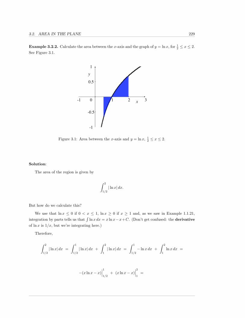
3.2. AREA IN THE PLANE 229
Example 3.2.2. Calculate the area between the x-axis and the graph of y = lnx, for 12 ≤ x ≤ 2.
See Figure 3.1.
-1 0 1 2 3
-1
-0.5
0.5
1
Figure 3.1: Area between the x-axis and y = lnx, 12 ≤ x ≤ 2.
Solution:
The area of the region is given by
∫ 2
1/2
| lnx| dx.
But how do we calculate this?
We use that lnx ≤ 0 if 0 < x ≤ 1, lnx ≥ 0 if x ≥ 1 and, as we saw in Example 1.1.21,integration by parts tells us that
∫lnx dx = x lnx−x+C. (Don’t get confused: the derivative
of lnx is 1/x, but we’re integrating here.)
Therefore,
∫ 2
1/2
| lnx| dx =∫ 1
1/2
| lnx| dx +∫ 2
1
| lnx| dx =∫ 1
1/2
− lnx dx +∫ 2
1
lnx dx =
−(x lnx− x)∣∣∣11/2
+ (x lnx− x)∣∣∣21
=
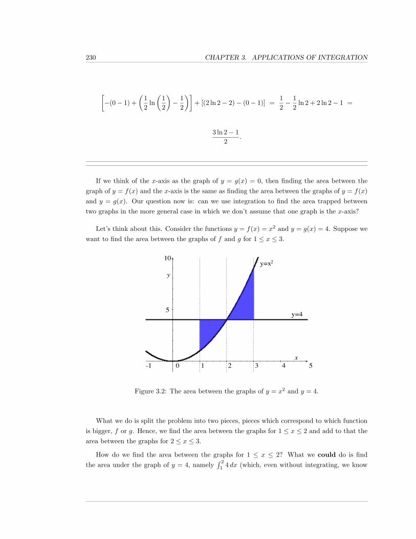
230 CHAPTER 3. APPLICATIONS OF INTEGRATION
[−(0− 1) +
(12
ln(
12
)− 1
2
)]+ [(2 ln 2− 2)− (0− 1)] =
12− 1
2ln 2 + 2 ln 2− 1 =
3 ln 2− 12
.
If we think of the x-axis as the graph of y = g(x) = 0, then finding the area between thegraph of y = f(x) and the x-axis is the same as finding the area between the graphs of y = f(x)and y = g(x). Our question now is: can we use integration to find the area trapped betweentwo graphs in the more general case in which we don’t assume that one graph is the x-axis?
Let’s think about this. Consider the functions y = f(x) = x2 and y = g(x) = 4. Suppose wewant to find the area between the graphs of f and g for 1 ≤ x ≤ 3.
-1 0 1 2 3 4 5
5
10
y=4
y=x2
Figure 3.2: The area between the graphs of y = x2 and y = 4.
What we do is split the problem into two pieces, pieces which correspond to which functionis bigger, f or g. Hence, we find the area between the graphs for 1 ≤ x ≤ 2 and add to that thearea between the graphs for 2 ≤ x ≤ 3.
How do we find the area between the graphs for 1 ≤ x ≤ 2? What we could do is findthe area under the graph of y = 4, namely
∫ 2
14 dx (which, even without integrating, we know
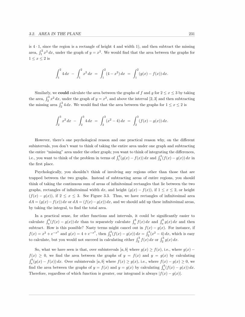
3.2. AREA IN THE PLANE 231
is 4 · 1, since the region is a rectangle of height 4 and width 1), and then subtract the missingarea,
∫ 2
1x2 dx, under the graph of y = x2. We would find that the area between the graphs for
1 ≤ x ≤ 2 is
∫ 2
1
4 dx −∫ 2
1
x2 dx =∫ 2
1
(4− x2) dx =∫ 2
1
(g(x)− f(x)) dx.
Similarly, we could calculate the area between the graphs of f and g for 2 ≤ x ≤ 3 by takingthe area,
∫ 3
2x2 dx, under the graph of y = x2, and above the interval [2, 3] and then subtracting
the missing area∫ 3
24 dx. We would find that the area between the graphs for 1 ≤ x ≤ 2 is
∫ 3
2
x2 dx −∫ 3
2
4 dx =∫ 3
2
(x2 − 4) dx =∫ 3
2
(f(x)− g(x)) dx.
However, there’s one psychological reason and one practical reason why, on the differentsubintervals, you don’t want to think of taking the entire area under one graph and subtractingthe entire “missing” area under the other graph; you want to think of integrating the differences,i.e., you want to think of the problem in terms of
∫ 2
1(g(x)− f(x)) dx and
∫ 3
2(f(x)− g(x)) dx in
the first place.
Psychologically, you shouldn’t think of involving any regions other than those that aretrapped between the two graphs. Instead of subtracting areas of entire regions, you shouldthink of taking the continuous sum of areas of infinitesimal rectangles that lie between the twographs, rectangles of infinitesimal width dx, and height (g(x) − f(x)), if 1 ≤ x ≤ 2, or height(f(x) − g(x)), if 2 ≤ x ≤ 3. See Figure 3.3. Thus, we have rectangles of infinitesimal areadA = (g(x)−f(x)) dx or dA = (f(x)− g(x)) dx, and we should add up these infinitesimal areas,by taking the integral, to find the total area.
In a practical sense, for other functions and intervals, it could be significantly easier tocalculate
∫ ba
(f(x) − g(x)) dx than to separately calculate∫ baf(x) dx and
∫ bag(x) dx and then
subtract. How is this possible? Nasty terms might cancel out in f(x) − g(x). For instance, iff(x) = x2 + e−x
2and g(x) = 4 + e−x
2, then
∫ 3
2(f(x)− g(x)) dx =
∫ 3
2(x2 − 4) dx, which is easy
to calculate, but you would not succeed in calculating either∫ 3
2f(x) dx or
∫ 3
2g(x) dx.
So, what we have seen is that, over subintervals [a, b] where g(x) ≥ f(x), i.e., where g(x)−f(x) ≥ 0, we find the area between the graphs of y = f(x) and y = g(x) by calculating∫ ba
(g(x) − f(x)) dx. Over subintervals [a, b] where f(x) ≥ g(x), i.e., where f(x) − g(x) ≥ 0, wefind the area between the graphs of y = f(x) and y = g(x) by calculating
∫ ba
(f(x) − g(x)) dx.Therefore, regardless of which function is greater, our integrand is always |f(x)− g(x)|.
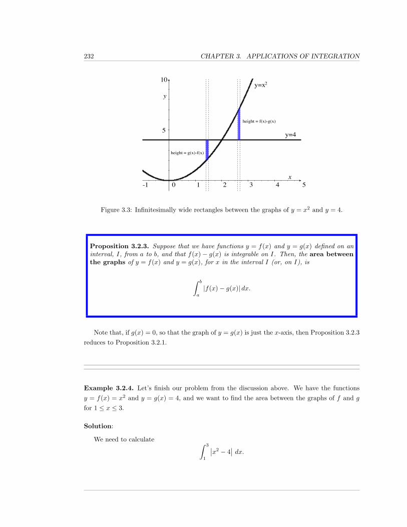
232 CHAPTER 3. APPLICATIONS OF INTEGRATION
-1 0 1 2 3 4 5
5
10
y=4
y=x2
height = g(x)-f(x)
height = f(x)-g(x)
Figure 3.3: Infinitesimally wide rectangles between the graphs of y = x2 and y = 4.
Proposition 3.2.3. Suppose that we have functions y = f(x) and y = g(x) defined on aninterval, I, from a to b, and that f(x)− g(x) is integrable on I. Then, the area betweenthe graphs of y = f(x) and y = g(x), for x in the interval I (or, on I), is
∫ b
a
|f(x)− g(x)| dx.
Note that, if g(x) = 0, so that the graph of y = g(x) is just the x-axis, then Proposition 3.2.3reduces to Proposition 3.2.1.
Example 3.2.4. Let’s finish our problem from the discussion above. We have the functionsy = f(x) = x2 and y = g(x) = 4, and we want to find the area between the graphs of f and g
for 1 ≤ x ≤ 3.
Solution:
We need to calculate ∫ 3
1
∣∣x2 − 4∣∣ dx.
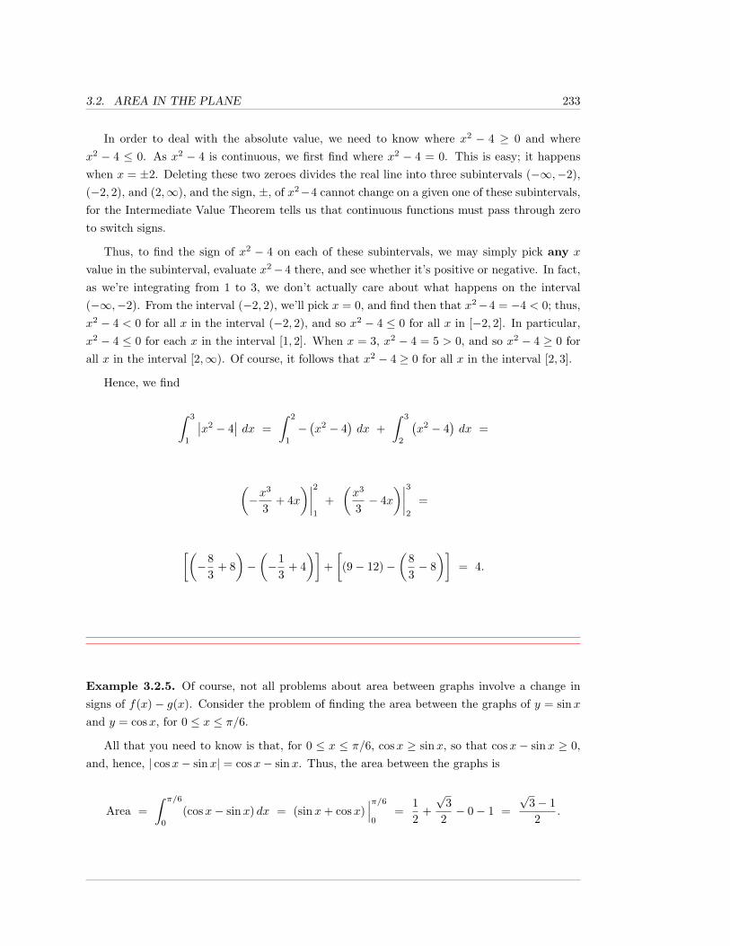
3.2. AREA IN THE PLANE 233
In order to deal with the absolute value, we need to know where x2 − 4 ≥ 0 and wherex2 − 4 ≤ 0. As x2 − 4 is continuous, we first find where x2 − 4 = 0. This is easy; it happenswhen x = ±2. Deleting these two zeroes divides the real line into three subintervals (−∞,−2),(−2, 2), and (2,∞), and the sign, ±, of x2−4 cannot change on a given one of these subintervals,for the Intermediate Value Theorem tells us that continuous functions must pass through zeroto switch signs.
Thus, to find the sign of x2 − 4 on each of these subintervals, we may simply pick any x
value in the subinterval, evaluate x2− 4 there, and see whether it’s positive or negative. In fact,as we’re integrating from 1 to 3, we don’t actually care about what happens on the interval(−∞,−2). From the interval (−2, 2), we’ll pick x = 0, and find then that x2−4 = −4 < 0; thus,x2 − 4 < 0 for all x in the interval (−2, 2), and so x2 − 4 ≤ 0 for all x in [−2, 2]. In particular,x2 − 4 ≤ 0 for each x in the interval [1, 2]. When x = 3, x2 − 4 = 5 > 0, and so x2 − 4 ≥ 0 forall x in the interval [2,∞). Of course, it follows that x2 − 4 ≥ 0 for all x in the interval [2, 3].
Hence, we find
∫ 3
1
∣∣x2 − 4∣∣ dx =
∫ 2
1
−(x2 − 4
)dx +
∫ 3
2
(x2 − 4
)dx =
(−x
3
3+ 4x
)∣∣∣∣21
+(x3
3− 4x
)∣∣∣∣32
=
[(−8
3+ 8)−(−1
3+ 4)]
+[(9− 12)−
(83− 8)]
= 4.
Example 3.2.5. Of course, not all problems about area between graphs involve a change insigns of f(x)− g(x). Consider the problem of finding the area between the graphs of y = sinxand y = cosx, for 0 ≤ x ≤ π/6.
All that you need to know is that, for 0 ≤ x ≤ π/6, cosx ≥ sinx, so that cosx − sinx ≥ 0,and, hence, | cosx− sinx| = cosx− sinx. Thus, the area between the graphs is
Area =∫ π/6
0
(cosx− sinx) dx = (sinx+ cosx)∣∣∣π/60
=12
+√
32− 0− 1 =
√3− 12
.
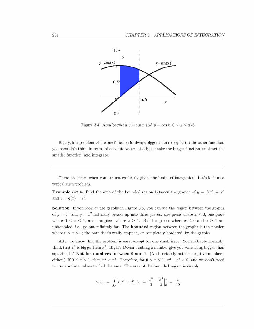
234 CHAPTER 3. APPLICATIONS OF INTEGRATION
-0.5
0
0.5
1
1.5
π/6
y=cos(x) y=sin(x)
Figure 3.4: Area between y = sinx and y = cosx, 0 ≤ x ≤ π/6.
Really, in a problem where one function is always bigger than (or equal to) the other function,you shouldn’t think in terms of absolute values at all; just take the bigger function, subtract thesmaller function, and integrate.
There are times when you are not explicitly given the limits of integration. Let’s look at atypical such problem.
Example 3.2.6. Find the area of the bounded region between the graphs of y = f(x) = x3
and y = g(x) = x2.
Solution: If you look at the graphs in Figure 3.5, you can see the region between the graphsof y = x3 and y = x2 naturally breaks up into three pieces: one piece where x ≤ 0, one piecewhere 0 ≤ x ≤ 1, and one piece where x ≥ 1. But the pieces where x ≤ 0 and x ≥ 1 areunbounded, i.e., go out infinitely far. The bounded region between the graphs is the portionwhere 0 ≤ x ≤ 1; the part that’s really trapped, or completely bordered, by the graphs.
After we know this, the problem is easy, except for one small issue. You probably normallythink that x3 is bigger than x2. Right? Doesn’t cubing a number give you something bigger thansquaring it? Not for numbers between 0 and 1! (And certainly not for negative numbers,either.) If 0 ≤ x ≤ 1, then x2 ≥ x3. Therefore, for 0 ≤ x ≤ 1, x2 − x3 ≥ 0, and we don’t needto use absolute values to find the area. The area of the bounded region is simply
Area =∫ 1
0
(x2 − x3) dx =x3
3− x4
4
∣∣∣10
=112.
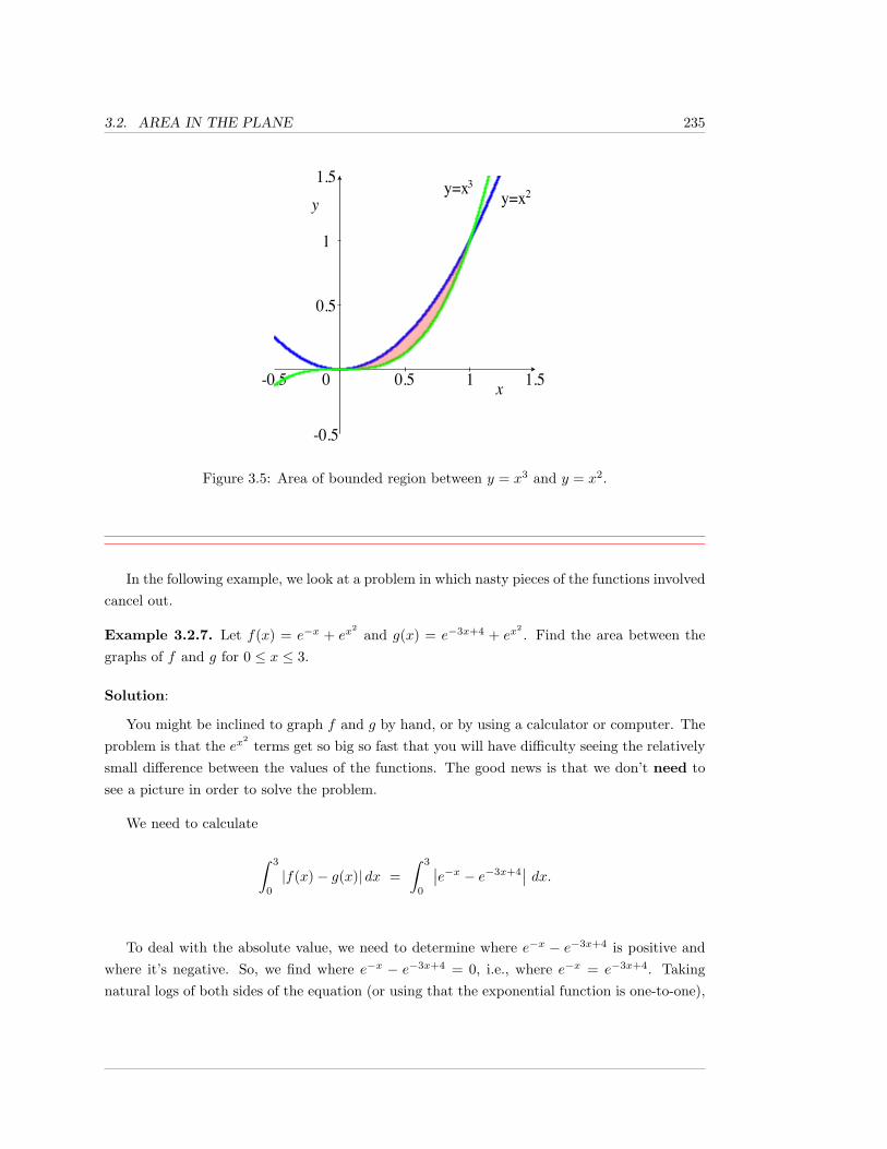
3.2. AREA IN THE PLANE 235
-0.5 0 0.5 1 1.5
-0.5
0.5
1
1.5 y=x3 y=x2
Figure 3.5: Area of bounded region between y = x3 and y = x2.
In the following example, we look at a problem in which nasty pieces of the functions involvedcancel out.
Example 3.2.7. Let f(x) = e−x + ex2
and g(x) = e−3x+4 + ex2. Find the area between the
graphs of f and g for 0 ≤ x ≤ 3.
Solution:
You might be inclined to graph f and g by hand, or by using a calculator or computer. Theproblem is that the ex
2terms get so big so fast that you will have difficulty seeing the relatively
small difference between the values of the functions. The good news is that we don’t need tosee a picture in order to solve the problem.
We need to calculate
∫ 3
0
|f(x)− g(x)| dx =∫ 3
0
∣∣e−x − e−3x+4∣∣ dx.
To deal with the absolute value, we need to determine where e−x − e−3x+4 is positive andwhere it’s negative. So, we find where e−x − e−3x+4 = 0, i.e., where e−x = e−3x+4. Takingnatural logs of both sides of the equation (or using that the exponential function is one-to-one),
236 CHAPTER 3. APPLICATIONS OF INTEGRATION
we find that −x = −3x+ 4, and so x = 2.
Therefore, since e−x − e−3x+4 is continuous and is zero only at x = 2, we must have thate−x − e−3x+4 is either always positive or always negative on each of the intervals (−∞, 2) and(2,∞). We simply check the sign of the function at some point in each interval. When x = 0,e−x−e−3x+4 = e0−e4 < 0; hence, e−x−e−3x+4 < 0 for all x in (−∞, 2), and so e−x−e−3x+4 ≤ 0for all x in (−∞, 2]. Similarly, when x = 3, e−x − e−3x+4 = e−3 − e−5 > 0, and we concludethat e−x − e−3x+4 ≥ 0 for all x in [2,∞).
Thus, we find
∫ 3
0
∣∣e−x − e−3x+4∣∣ dx =
∫ 2
0
∣∣e−x − e−3x+4∣∣ dx +
∫ 3
2
∣∣e−x − e−3x+4∣∣ dx =
∫ 2
0
−(e−x − e−3x+4
)dx +
∫ 3
2
(e−x − e−3x+4
)dx.
Let’s produce an anti-derivative for all functions of the form eax+b, so that we can use thisresult to integrate each piece in the integrals above. Consider
∫eax+b dx, where a and b are
constants, and a 6= 0. Make the substitution u = ax + b, so that du = a dx, i.e., dx = du/a.Then, we find
∫eax+b dx =
∫eu · du
a=
1a
∫eu du =
1aeu + C =
eax+b
a+ C.
Now, we apply this formula to e−x and e−3x+4, and obtain
∫ 2
0
−(e−x − e−3x+4
)dx = e−x − e−3x+4
3
∣∣∣∣20
= e−2 − e−2
3−(
1− e4
3
)=
2e−2
3− 1 +
e4
3.
We also find that
∫ 3
2
(e−x − e−3x+4
)dx = −e−x +
e−3x+4
3
∣∣∣∣32
=
3.2. AREA IN THE PLANE 237
−e−3 +e−5
3−(−e−2 +
e−2
3
)= −e−3 +
e−5
3+
2e−2
3.
Putting together all of our above work, we find:
Area =∫ 3
0
∣∣e−x − e−3x+4∣∣ dx =
2e−2
3− 1 +
e4
3− e−3 +
e−5
3+
2e−2
3=
e4 + 4e−2 + e−5
3− e−3 − 1.
In the next example, we consider the same two functions that we did above, but now we lookat the area of an unbounded region, a region that extends out infinitely far. This, of course,leads to an improper integral.
Example 3.2.8. Let f(x) = e−x + ex2
and g(x) = e−3x+4 + ex2. Find the area between the
graphs of f and g for 0 ≤ x <∞.
Solution:
These are the same functions that we used in the previous example, and so we can use muchof our work from that problem.
We need to calculate ∫ ∞0
∣∣e−x − e−3x+4∣∣ dx.
We could do this either one of two ways.
First, we could proceed exactly as we did in the previous example, and write
∫ ∞0
∣∣e−x − e−3x+4∣∣ dx =
∫ 2
0
∣∣e−x − e−3x+4∣∣ dx +
∫ ∞2
∣∣e−x − e−3x+4∣∣ dx =
∫ 2
0
−(e−x − e−3x+4
)dx +
∫ ∞2
(e−x − e−3x+4
)dx.
We already calculated, in the previous example, the integral on the left; we would still need tocalculate the improper integral on the right.
238 CHAPTER 3. APPLICATIONS OF INTEGRATION
However, given that we already calculated∫ 3
0
∣∣e−x − e−3x+4∣∣ dx is the previous example, it
would also be reasonable to split the integral up in the following manner:
∫ ∞0
∣∣e−x − e−3x+4∣∣ dx =
∫ 3
0
∣∣e−x − e−3x+4∣∣ dx +
∫ ∞3
∣∣e−x − e−3x+4∣∣ dx =
e4 + 4e−2 + e−5
3− e−3 − 1 +
∫ ∞3
(e−x − e−3x+4
)dx,
where, again, we still need to calculate the improper integral on the right.
We’ll use the second splitting of the integral, though it makes little difference. We find
∫ ∞3
(e−x − e−3x+4
)dx = lim
p→∞
{−e−x +
e−3x+4
3
∣∣∣∣p3
}.
limp→∞
(−e−p +
e−3p+4
3+ e−3 − e−5
3
)= e−3 − e−5
3.
Therefore, our final answer is
Area =∫ ∞
0
∣∣e−x − e−3x+4∣∣ dx =
e4 + 4e−2 + e−5
3− e−3 − 1 + e−3 − e−5
3=
e4 + 4e−2
3− 1.
What if you want to find the area between curves that aren’t given to you by having y interms of x, but instead are given to you by x being specified in terms of y? For instance, howdo you find the area between the curves/lines x = 4− y2 and x = 2− y for 0 ≤ y ≤ 2?
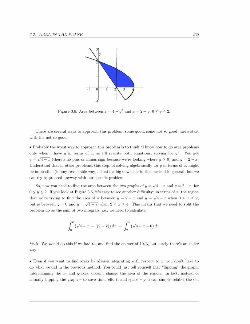
3.2. AREA IN THE PLANE 239
-1 0 1 2 3 4
-1
1
2
3
Figure 3.6: Area between x = 4− y2 and x = 2− y, 0 ≤ y ≤ 2.
There are several ways to approach this problem, some good, some not so good. Let’s startwith the not so good.
• Probably the worst way to approach this problem is to think “I know how to do area problemsonly when I have y in terms of x, so I’ll rewrite both equations, solving for y”. You gety =√
4− x (there’s no plus or minus sign because we’re looking where y ≥ 0) and y = 2 − x.Understand that in other problems, this step, of solving algebraically for y in terms of x, mightbe impossible (in any reasonable way). That’s a big downside to this method in general, but wecan try to proceed anyway with our specific problem.
So, now you need to find the area between the two graphs of y =√
4− x and y = 2− x, for0 ≤ y ≤ 2. If you look at Figure 3.6, it’s easy to see another difficulty: in terms of x, the regionthat we’re trying to find the area of is between y = 2 − x and y =
√4− x when 0 ≤ x ≤ 2,
but is between y = 0 and y =√
4− x when 2 ≤ x ≤ 4. This means that we need to split theproblem up as the sum of two integrals, i.e., we need to calculate
∫ 2
0
(√4− x − (2− x)
)dx +
∫ 4
2
(√4− x− 0
)dx.
Yuck. We would do this if we had to, and find the answer of 10/3, but surely there’s an easierway.
• Even if you want to find areas by always integrating with respect to x, you don’t have todo what we did in the previous method. You could just tell yourself that “flipping” the graph,interchanging the x- and y-axes, doesn’t change the area of the region. In fact, instead ofactually flipping the graph – to save time, effort, and space – you can simply relabel the old
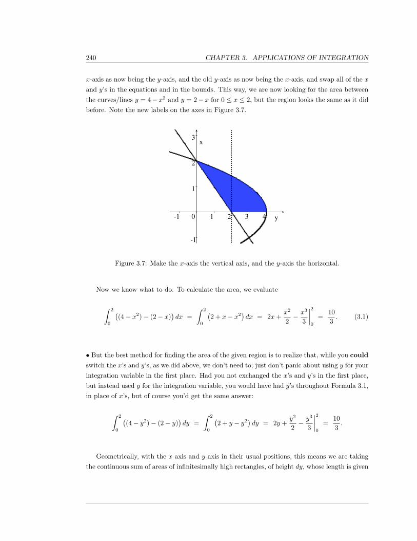
240 CHAPTER 3. APPLICATIONS OF INTEGRATION
x-axis as now being the y-axis, and the old y-axis as now being the x-axis, and swap all of the xand y’s in the equations and in the bounds. This way, we are now looking for the area betweenthe curves/lines y = 4− x2 and y = 2− x for 0 ≤ x ≤ 2, but the region looks the same as it didbefore. Note the new labels on the axes in Figure 3.7.
-1 0 1 2 3 4
-1
1
2
3 x
y
Figure 3.7: Make the x-axis the vertical axis, and the y-axis the horizontal.
Now we know what to do. To calculate the area, we evaluate
∫ 2
0
((4− x2)− (2− x)
)dx =
∫ 2
0
(2 + x− x2
)dx = 2x+
x2
2− x3
3
∣∣∣∣20
=103. (3.1)
• But the best method for finding the area of the given region is to realize that, while you could
switch the x’s and y’s, as we did above, we don’t need to; just don’t panic about using y for yourintegration variable in the first place. Had you not exchanged the x’s and y’s in the first place,but instead used y for the integration variable, you would have had y’s throughout Formula 3.1,in place of x’s, but of course you’d get the same answer:
∫ 2
0
((4− y2)− (2− y)
)dy =
∫ 2
0
(2 + y − y2
)dy = 2y +
y2
2− y3
3
∣∣∣∣20
=103.
Geometrically, with the x-axis and y-axis in their usual positions, this means we are takingthe continuous sum of areas of infinitesimally high rectangles, of height dy, whose length is given
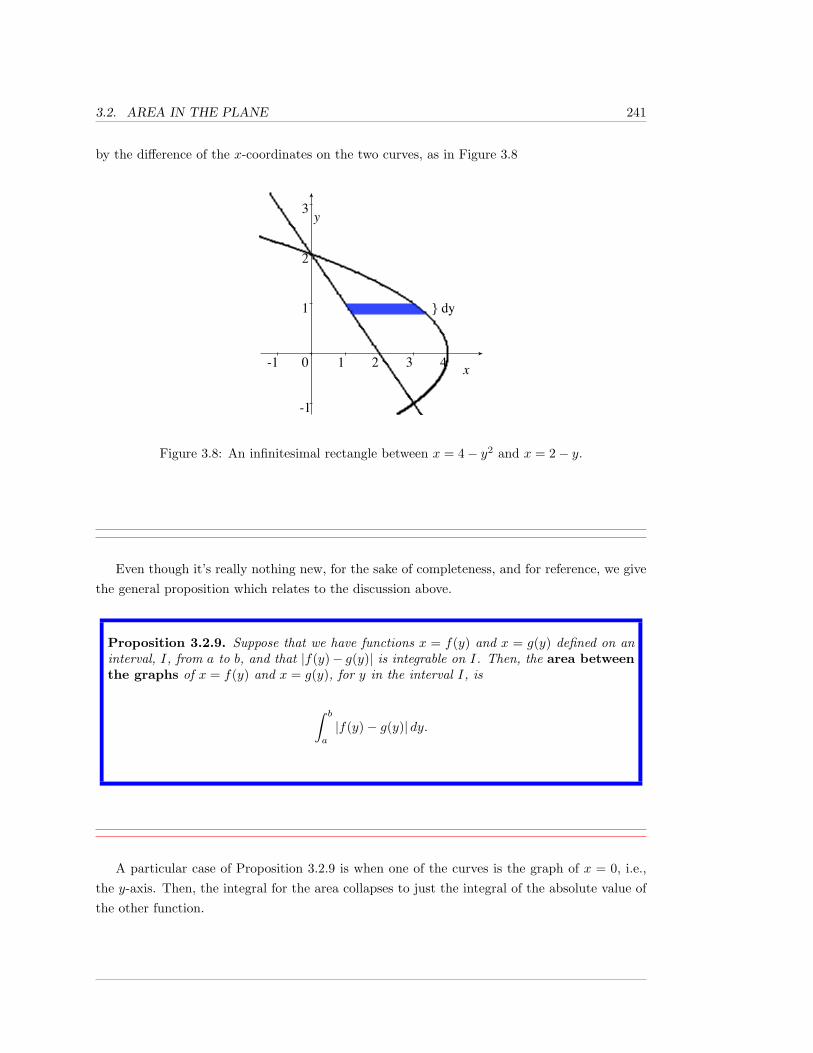
3.2. AREA IN THE PLANE 241
by the difference of the x-coordinates on the two curves, as in Figure 3.8
-1 0 1 2 3 4
-1
1
2
3
} dy
Figure 3.8: An infinitesimal rectangle between x = 4− y2 and x = 2− y.
Even though it’s really nothing new, for the sake of completeness, and for reference, we givethe general proposition which relates to the discussion above.
Proposition 3.2.9. Suppose that we have functions x = f(y) and x = g(y) defined on aninterval, I, from a to b, and that |f(y)− g(y)| is integrable on I. Then, the area betweenthe graphs of x = f(y) and x = g(y), for y in the interval I, is
∫ b
a
|f(y)− g(y)| dy.
A particular case of Proposition 3.2.9 is when one of the curves is the graph of x = 0, i.e.,the y-axis. Then, the integral for the area collapses to just the integral of the absolute value ofthe other function.
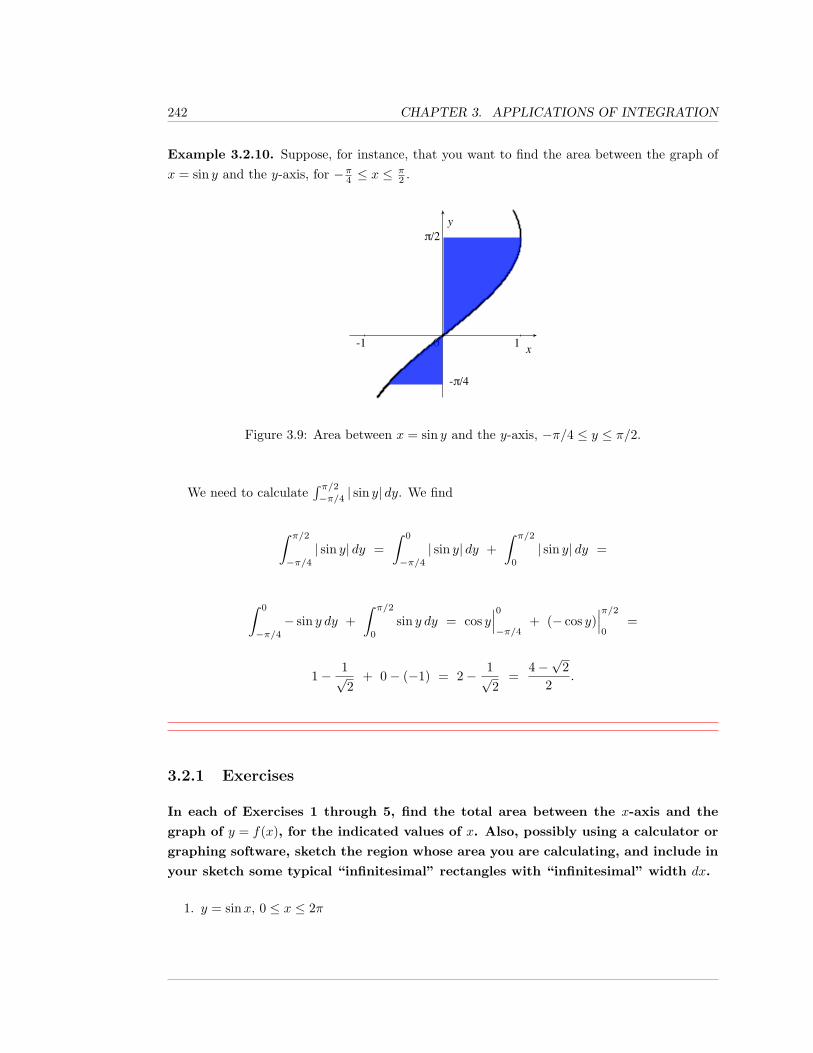
242 CHAPTER 3. APPLICATIONS OF INTEGRATION
Example 3.2.10. Suppose, for instance, that you want to find the area between the graph ofx = sin y and the y-axis, for −π4 ≤ x ≤
π2 .
-1 0 1
-π/4
π/2
Figure 3.9: Area between x = sin y and the y-axis, −π/4 ≤ y ≤ π/2.
We need to calculate∫ π/2−π/4 | sin y| dy. We find
∫ π/2
−π/4| sin y| dy =
∫ 0
−π/4| sin y| dy +
∫ π/2
0
| sin y| dy =
∫ 0
−π/4− sin y dy +
∫ π/2
0
sin y dy = cos y∣∣∣0−π/4
+ (− cos y)∣∣∣π/20
=
1− 1√2
+ 0− (−1) = 2− 1√2
=4−√
22
.
3.2.1 Exercises
In each of Exercises 1 through 5, find the total area between the x-axis and the
graph of y = f(x), for the indicated values of x. Also, possibly using a calculator or
graphing software, sketch the region whose area you are calculating, and include in
your sketch some typical “infinitesimal” rectangles with “infinitesimal” width dx.
1. y = sinx, 0 ≤ x ≤ 2π
3.2. AREA IN THE PLANE 243
2. y = cosx, 0 ≤ x ≤ 2π
3. y = 9− x2, −4 ≤ x ≤ 2
4. y = x3 + x2 − 2x, −3 ≤ x ≤ 2
5. y = xe(x2), −1 ≤ x ≤ 1
In each of Exercises 6 through 10, find the area between the y-axis and the graph of
x = f(y), for the indicated values of y. Also, possibly using a calculator or graphing
software, sketch the region whose area you are calculating, and include in your
sketch some typical “infinitesimal” rectangles with “infinitesimal” height dy.
6. x = sin y, 0 ≤ y ≤ 2π
7. x = cos y, 0 ≤ y ≤ 2π
8. x = 9− y2, −4 ≤ y ≤ 2
9. x = y3 + y2 − 2y, −3 ≤ y ≤ 2
10. x = ye(y2), −1 ≤ y ≤ 1
In each of Exercises 11 through 20, find the area of the bounded region between
the graphs of the two given functions. Use integration with respect to whichever
variable seems most convenient.
11. y = 3− x2, y = −6
12. y = 3− x2, y = 3x− 1
13. x = 3− y2, x = 3y − 1
14. x = y2, y = x2
15. y = x(ex − e), y = 0
16. x = y(ey − e), x = 0
17. x =4
1 + y2, x = 2
18. y =10
1 + x2, y = 2
19. y =10
1 + x2, y = 1− 7
1 + x2
244 CHAPTER 3. APPLICATIONS OF INTEGRATION
20. x =10
1 + y2, x = 1− 7
1 + y2
In each of Exercises 21 through 36, calculate the total area bounded by the graphs
of y = f(x) and y = g(x), or x = f(y) and x = g(y), for values of the independent
variable in the given interval.
21. f(x) = x2 − 16, g(x) = 9, [−10, 10].
22. f(x) = sinx, g(x) = cosx, [0, 2π].
23. f(y) = sin y, g(y) = sin 2y, [0, 2π].
24. f(y) = ey2
+ e3y+1, g(y) = e2y+2 + ey2, [−4, 3].
25. f(x) = x4 + x3 − 3x2 + 5x+ 5, g(x) = x4 + 2x3 − 3x2 + 5x+ 6, [−4, 6].
26. f(x) = ln(xx tanx)− ln(sinx), g(x) = ln(ex cosx), [1, 3].
27. f(y) = 3/(y + 2), g(y) = 2/(y − 4), [−1, 3].
28. f(y) =tan y
1− tan y tan 1, g(y) =
− tan 11− tan y tan 1
, [0, π/4].
29. f(x) = x4 + x2 + 2, g(x) = x3 + 3x, [−3, 3].
30. f(x) = tan−1 x+ x2 + 3, g(x) = 2x2 + x+ tan−1 x− 4, [−3, 5].
31. f(y) = e2y + 4, g(y) = e−2y + 2, [−5, 5].
32. f(y) =y4 + y2√y6 + y4
, g(y) =y2√y2 + 1
, [1, 4].
33. f(x) = sinh−1 x, g(x) = cosh−1 x, [1, 10].
34. f(x) =x2
(x− 2)(x+ 2), g(x) =
4(x− 2)(x+ 2)
, [−1, 1].
35. f(y) = |y|, g(y) = −|y|+ 1, [−1/2, 1/2].
36. f(y) = 2y, g(y) = 3y, [−1, 2].
37. Prove that if f , g and h are continuous functions on [a, b] then the area between the graphsof f and g is equal to the area between the graphs of f + h and g + h.
38. Suppose the area enclosed by two continuous functions f and g on the interval [a, b] isA =
∫ ba|f(x) − g(x)| dx. Suppose c is an arbitrary real number. Is it true that the area
between the graphs of cf(x) and cg(x) is cA? If not, how can you correct this statement?
3.2. AREA IN THE PLANE 245
39. Calculate the limiting area between the curves e−at and e−bt between t = 0 and t = U
where U →∞. Assume a and b are positive distinct real numbers.
40. Calculate the area between the curves h(y) = ln ay and g(y) = ln by on the interval [c, d]where a, b and c are positive and a 6= b.
41. Calculate the area between the curves a(t) = 1/t and b(t) = 1/t2 on the interval [1, U ].Does the limiting area converge as U →∞?
42. Redo the previous problem with a(t) = 1/t2 and b(t) = 1/t3.
43. What is the area enclosed by the curves f(x) = sinnx and g(x) = cosnx on the interval[0, 2π] where n is a positive integer?
In each of Exercises 44 through 47, use the Midpoint Rule to approximate the areas
bound by the two curves on the interval [0, 1]. Use a partition of n = 4 evenly spaced
points.
44. f(x) = ex2, g(x) = ex.
45. f(x) = exk
, g(x) = ex, k > 0.
46. f(x) = exk
, g(x) = exm
, k,m > 0.
47. f(x) =√
1 + x3, g(x) = x+ 1.
In Exercises 48 through 51, you are given the area A between the graphs of f(x)and g(x) over an interval I. You are also given the two functions with one unknown
parameter c. Solve for the parameter.
48. A = 24, f(x) = 2x2 − 3x+ 4, g(x) = x2 + cx− 6, I = [0, 6].
49. A = −2 + 2√
3− π/6, f(x) = sinx, g(x) = c, I = [0, π], c > 0.
50. A = 16, f(x) = c− |x|, g(x) = |x|, I = [−c, c].
51. A = 9π − 18, f(x) =√c2 − x2, g(x) = c− x, I = [0, c].
52. The equation h(x) =√
1− x2 defines a semi-circle of radius one. Let j(x) = C be theequation of a horizontal line. Find the value of C such that the line j(x) splits the semi-circle into two sections with equal areas.
53. Suppose that f is continuous on [a, b].
a. Prove that |f | is integrable on [a, b].
246 CHAPTER 3. APPLICATIONS OF INTEGRATION
b. Argue that one can choose k = ±1 such that k∫ baf(x) dx ≥ 0.
c. Conclude that∣∣∣∫ ba f(x) dx
∣∣∣ ≤ ∫ ba |f(x)| dx.
d. Use part (c) to show that a lower bound for the area enclosed between the graphs off(x) and g(x) on the interval [a, b] is
∣∣∣∫ ba f(x) dx−∫ bag(x) dx
∣∣∣.54. Argue that if f and h are continuous on [a, b], then the area enclosed by f and the x-axis
is less than or equal to the sum of the area enclosed by f and h, and the area enclosed by
h and the x-axis.
55. Suppose f and g are continuous on [a, b]. Let h(x) = |f(x)| and j(x) = |g(x)|. Prove thatthe area enclosed by j and h on the interval [a, b] is less than or equal to the area enclosedby f and g on the interval [a, b].
It’s often more convenient to describe a function f using polar coordinates. If we
assume that the distance from the origin to a point on the graph, r, depends only
on the angle between the x-axis and ray connecting the origin to the point, θ then
we can write r = f(θ). Under reasonable assumptions, the area of the polar region
defined for θ ∈ [a, b] is A =12
∫ b
a
f2(θ) dθ. Here, we assume that b− a ≤ 2π to prevent
double counting. Calculate the areas of the polar regions in Exercises 36 - 40.
56. r = θ, θ ∈ [0, π].
57. r = sin 3θ, θ ∈ [0, π/3].
58. 4 = sinnθ, θ ∈ [0, π/n], n a positive integer.
59. r = r0, θ ∈ [0, 2π]. What familiar shape is this?
60. r = 1 + sin θ, θ ∈ [0, 2π].
The area between two polar regions defined by the functions r1(θ) and r2(θ) is given
by A = 12
∫ ba|r1(θ) − r2(θ)| dθ. Calculate the areas between the polar curves over the
given angular interval in Exercises 41 - 45
61. r1(θ) = 1/2, r2(θ) = cos 3θ, I = [−π/9, π/9].
62. r1(θ) = 3 cos θ, r2(θ) = 1 + cos θ, θ ∈ [−π/3, π/3].
63. r1 = sin θ, r2 = cos θ, I = [0, π/4].
64. Recalculate the previous problem by writing the equations of the graphs of the two func-tions in cartesian coordinates.
3.2. AREA IN THE PLANE 247
65. Use the polar area formula to find the area of the annular region enclosed by circles ofradii R1 and R2, 0 < R1 < R2.
Recall that the area below the graph of a probability density function (pdf) is
interpreted as a probability. Specifically, if f(x) is a pdf of a random variable
X, then the probability that X is between a and b is∫ b
a
f(x) dx. In finance and
economics, the area between two curves can be used to assess the materiality in
choosing one model over another. We explore this idea in Exercises 46 - 48.
66. Suppose that the XY Z corporation is considering a $200,000 investment. It is knownwith certainty that the most XY Z can lose is its initial investment of $200,000 and themost it can profit is $700,000. Analyst A believes the profit is uniformly distributedon the interval [−200000, 700000]. Analyst B believes the profit has density function
f2(x) =x2
117, 000, 000.
a. What is f1(x), the pdf based on Analyst A’s assumptions?
b. What is the area between f1(x) and f2(x) on the interval [500, 700]? What is theprobabilistic interpretation of this area?
67. Under which analyst’s assumptions is it more likely for XY Z to experience a positiveprofit from this investment?
68. Calculate the area between the graphs of the functions xf1(x) and xf2(x) on the interval[−200, 700]. What does this area represent?
69. Suppose f(x) is a strictly increasing continuous function defined on all reals with the
property that f(0) = 0. Then f possesses an inverse function g. Just as∫ a
0
f(x) dx is the
area below the graph of f on the interval [0, a],∫ b
0
g(y) dy is the area to the left of the
graph of g along the (vertical) interval [0, b].
a. Assume a and b are positive. Draw a picture to prove that
ab ≤∫ a
0
f(x) dx+∫ b
0
g(y) dy.
This is Young’s Inequality.
b. Based on the picture, formulate a conjecture about when the inequality is an equality.
248 CHAPTER 3. APPLICATIONS OF INTEGRATION
70. Use the previous problem and the function f(x) = xk, k > 0 to prove that
ab ≤ ap
p+bq
q
if a, b ≥ 0, 1 < p and1p
+1q
= 1.
71. a. Suppose f and g are two continuous functions, both of which are positive for all real
x. Suppose p > 1 is a real number, and q is the unique real such that1p
+1q
= 1.
Suppose f and g have the additional properties:
(∫ b
a
[f(x)]p dx
)1/p
= 1 and
(∫ b
a
[g(x)]q dx
)1/q
= 1.
Integrate both sides of the inequality in the previous problem to prove that
∫ b
a
f(x)g(x) dx ≤ 1.
b. Now suppose f and g satisfy all the conditions in part (a) except the last two. Provethat ∫ b
a
f(x)g(x) dx ≤
(∫ b
a
[f(x)]p dx
)1/p
·
(∫ b
a
[g(x)]q dx
)1/q
.
This result is known as Holder’s Inequality.
3.3. DISTANCE TRAVELED IN SPACE AND ARC LENGTH 249
3.3 Distance Traveled in Spaceand Arc Length
In Section 3.1, we looked at an object which was moving in a straight line, and found that itsdisplacement and distance traveled could be calculated by integrating its velocity v(t) and thespeed |v(t)|, respectively.
Suppose, however, that an object is moving along some curved path in a plane or in space.How do we use the velocity and/or speed of the object to calculate the displacement and thedistance traveled? Amazingly, the answer is that, aside from writing things in terms of vectors,the formulas look exactly the same.
It’s also true that the total distance traveled by an object is equal to the length of the curve(or line) that it travels along, provided that the object doesn’t move back over points that it’salready hit. This means that we can use the same techniques to calculate the arc length of acurve that we use in calculating the distance traveled.
In this section, we will use a small amount of material on vectors and vector-valued functions,such as the material in Appendix A. While this discussion could be put off until you take multi-variable Calculus, it is really not much more difficult than analyzing motion in a straight line.
Displacement and distance traveled:
Suppose that an object is moving in xyz-space, R3, in such a way that, at time t, its x-, y-,and z-coordinates are given by continuously differentiable functions x(t), y(t), z(t). Then, theposition function or position vector or, simply, position of the object at time t is
~p(t) = (x(t), y(t), z(t)).
When we say that ~p : [a, b] → R3 is continuously differentiable, you may wonder what ismeant at the endpoints a and b of the closed interval, since you can’t take two-sided limitsthere. We shall always mean that ~p is defined and differentiable on an open interval whichcontains [a, b], and that ~p ′ is continuous when restricted to the closed interval [a, b].
For a given t value, we sometimes think of ~p(t) as simply the point (x(t), y(t), z(t)), and, atother times, think of ~p(t) as the vector which is represented by the arrow from the origin to thepoint ~p(t); the context should always make it clear how we are thinking of ~p(t).
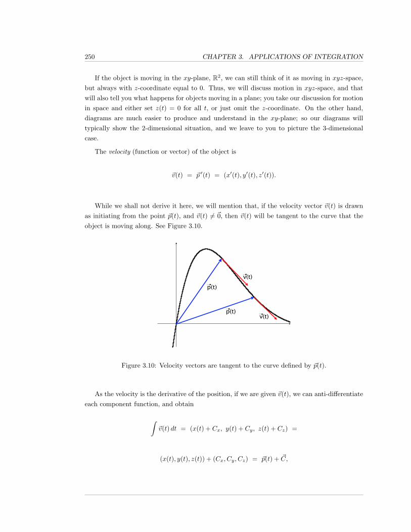
250 CHAPTER 3. APPLICATIONS OF INTEGRATION
If the object is moving in the xy-plane, R2, we can still think of it as moving in xyz-space,but always with z-coordinate equal to 0. Thus, we will discuss motion in xyz-space, and thatwill also tell you what happens for objects moving in a plane; you take our discussion for motionin space and either set z(t) = 0 for all t, or just omit the z-coordinate. On the other hand,diagrams are much easier to produce and understand in the xy-plane; so our diagrams willtypically show the 2-dimensional situation, and we leave to you to picture the 3-dimensionalcase.
The velocity (function or vector) of the object is
~v(t) = ~p ′(t) = (x′(t), y′(t), z′(t)).
While we shall not derive it here, we will mention that, if the velocity vector ~v(t) is drawnas initiating from the point ~p(t), and ~v(t) 6= ~0, then ~v(t) will be tangent to the curve that theobject is moving along. See Figure 3.10.
p(t)
p(t)
v(t)
v(t)
Figure 3.10: Velocity vectors are tangent to the curve defined by ~p(t).
As the velocity is the derivative of the position, if we are given ~v(t), we can anti-differentiateeach component function, and obtain
∫~v(t) dt = (x(t) + Cx, y(t) + Cy, z(t) + Cz) =
(x(t), y(t), z(t)) + (Cx, Cy, Cz) = ~p(t) + ~C,
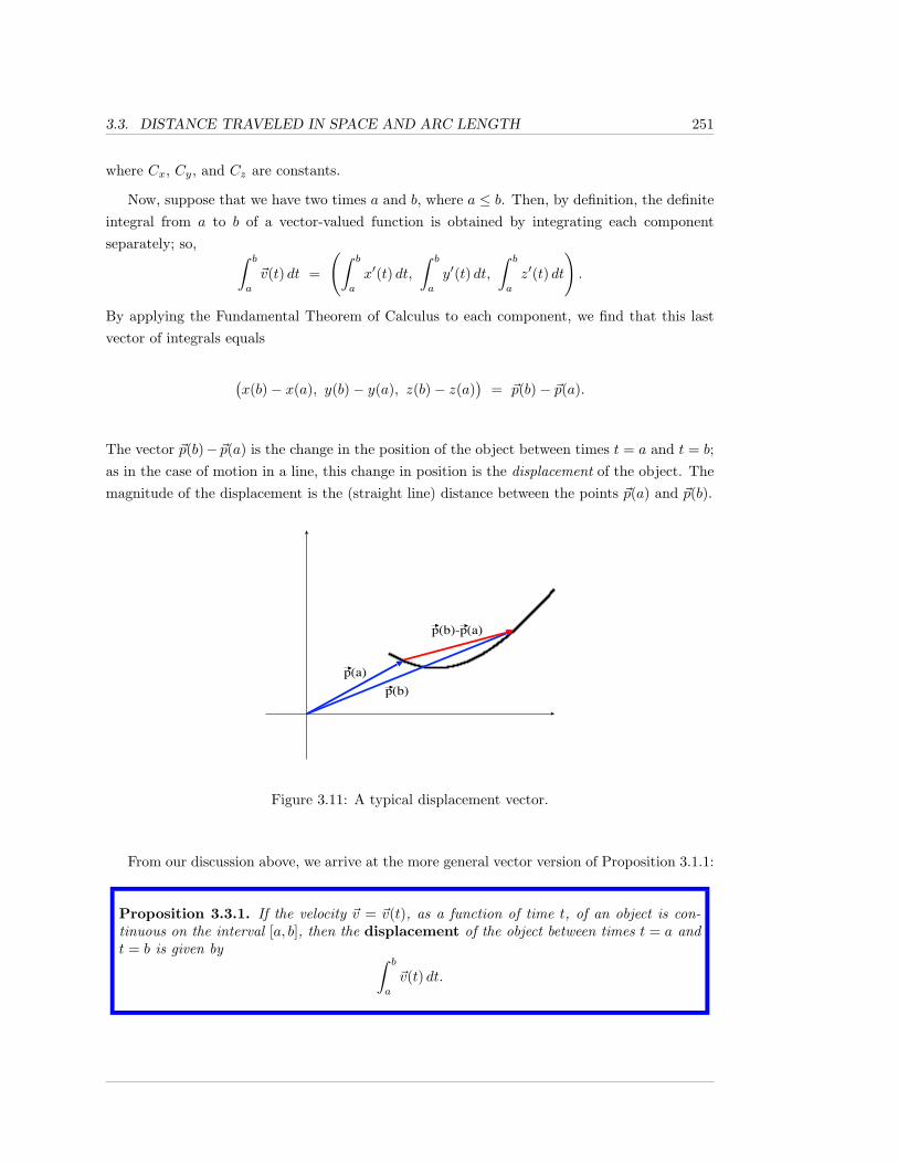
3.3. DISTANCE TRAVELED IN SPACE AND ARC LENGTH 251
where Cx, Cy, and Cz are constants.
Now, suppose that we have two times a and b, where a ≤ b. Then, by definition, the definiteintegral from a to b of a vector-valued function is obtained by integrating each componentseparately; so, ∫ b
a
~v(t) dt =
(∫ b
a
x′(t) dt,∫ b
a
y′(t) dt,∫ b
a
z′(t) dt
).
By applying the Fundamental Theorem of Calculus to each component, we find that this lastvector of integrals equals
(x(b)− x(a), y(b)− y(a), z(b)− z(a)
)= ~p(b)− ~p(a).
The vector ~p(b)− ~p(a) is the change in the position of the object between times t = a and t = b;as in the case of motion in a line, this change in position is the displacement of the object. Themagnitude of the displacement is the (straight line) distance between the points ~p(a) and ~p(b).
p(a)p(b)
p(b)-p(a)
Figure 3.11: A typical displacement vector.
From our discussion above, we arrive at the more general vector version of Proposition 3.1.1:
Proposition 3.3.1. If the velocity ~v = ~v(t), as a function of time t, of an object is con-tinuous on the interval [a, b], then the displacement of the object between times t = a andt = b is given by ∫ b
a
~v(t) dt.
252 CHAPTER 3. APPLICATIONS OF INTEGRATION
Example 3.3.2. A particle’s velocity is given by ~v(t) = (et,√
2,−e−t) meters per second, wheret is in seconds. What is the displacement of the particle between times t = 0 and t = 1 seconds?What is the magnitude of the displacement?
Solution:
This is easy. We find the displacement is
~p(1)− ~p(0) =∫ 1
0
~v(t) dt =∫ 1
0
(et,√
2,−e−t) dt = (et,√
2 t, e−t)∣∣∣10
=
(e,√
2, e−1)− (1, 0, 1) = (e− 1,√
2, e−1 − 1) meters.
The magnitude |~p(1)− ~p(0)| of the displacement vector is
|~p(1)− ~p(0)| =∣∣(e,√2, e−1)− (1, 0, 1)
∣∣ =√
(e− 1)2 + (√
2)2 + (e−1 − 1)2 =
√e2 − 2e+ 1 + 2 + e−2 − 2e−1 + 1 =
√(e− e−1)2 − 2(e+ e−1 − 3) meters,
where we have left the answer in this form for a reason that will be apparent in the next example.
If we look at the example above, and anti-differentiate ~v(t), we find that the position ~p(t) isgiven by
~p(t) = (et,√
2 t, e−t) + ~C,
where ~C is a constant vector. This means that, between times 0 and 1 second, the particlemoves from the point (1, 0, 1) + ~C to the point (e,
√2, e−1) + ~C, not along a straight line, but
rather along the curved path ~p(t) = (et,√
2 t, e−t) + ~C.
The (straight line) distance between the initial and final points of the particle is the distancebetween (e,
√2, e−1) + ~C and (1, 0, 1) + ~C; this is equal to the magnitude of the displacement
|~p(1)− ~p(0)|.
But, what if we want to know the total distance traveled by the particle along the curved
path given by ~p(t) = (et,√
2 t, e−t) + ~C? This distance traveled along the curved path should
(and will) turn out to be bigger than√
(e+ e−1)2 − 2(e+ e−1 − 3).
3.3. DISTANCE TRAVELED IN SPACE AND ARC LENGTH 253
To determine how to calculate the distance traveled by an object, first think about approx-imating the distance traveled during a small interval of time, and then we add together theresulting small distances, and take the limit as the size of the time interval approaches zero.Not surprisingly, this results in an integral.
Suppose that we have two times t0 < t1, and let’s think about what happens when ∆t = t1−t0is small (close to 0). If ∆t is close to 0, then the distance ∆s that the object travels (along itspossibly curved path) should approximately equal the distance along a straight line between thestarting position ~p(t0) and the ending position ~p(t1); this straight line distance is |~p(t1)− ~p(t0)|.Thus, we have
∆s ≈ |~p(t1)− ~p(t0)|.
We can rewrite this distance as
∆s ≈∣∣∣∣~p(t0 + ∆t)− ~p(t0)
∆t
∣∣∣∣ ∆t,
where we used that ∆t is positive. As ∆t→ 0,(~p(t0 +∆t)−~p(t0)
)/∆t approaches ~v(t) = ~p ′(t0).
Using differential notation and infinitesimal terminology, this means that the infinitesimaldistance ds traveled by the object in the infinitesimal time interval dt is
ds = |~v(t)| dt.
The infinitesimal value ds is frequently referred to an element of arc length. Of course, to obtainthe total distance traveled, we take a continuous sum of the infinitesimal distances traveled, i.e.,we take an integral.
Proposition 3.3.3. If the velocity ~v = ~v(t), as a function of time t, of an object is contin-uous on the interval [a, b], then the distance traveled by the object between times t = aand t = b is given by ∫ t=b
t=a
ds =∫ b
a
|~v(t)| dt,
where ds = |~v(t)| dt.
254 CHAPTER 3. APPLICATIONS OF INTEGRATION
Example 3.3.4. Let’s return to the situation in Example 3.3.2. A particle’s velocity is givenby ~v(t) = (et,
√2,−e−t) meters per second, where t is in seconds. What is the distance traveled
by the particle between times t = 0 and t = 1 seconds?
Solution:
We calculate that the distance traveled:
∫ 1
0
|~v(t)| dt =∫ 1
0
√(et)2 + (
√2)2 + (−e−t)2 dt =
∫ 1
0
√e2t + 2 + e−2t dt =
∫ 1
0
√(et + e−t)2 dt =
∫ 1
0
(et + e−t) dt =(et − e−t
) ∣∣∣10
= (e− e−1)− (1− 1) =
e− e−1 meters.
Note that, since e + e−1 − 3 > 0, the distance traveled is greater than the magnitude of thedisplacement, √
(e− e−1)2 − 2(e+ e−1 − 3) meters,
which we found in Example 3.3.2. In other words, the distance traveled along a curved pathbetween two points is greater than the straight line distance between the points. Good!
If the velocity ~v(t) of an object is continuous on the interval [a, b], then we may define thedistance traveled function between times a and t, where a ≤ t ≤ b, to be
s(t) =∫ t
a
|~v(z)| dz,
where z is just a dummy variable, which we introduce since t is now a limit of integration.
Then, the first part of the Fundamental Theorem of Calculus, Theorem 2.4.7, tells us that
ds
dt= |~v(t)|.
Definition 3.3.5. The speed of an object, whose velocity function is continuous, is themagnitude of the velocity or, equivalently, the rate of change of the distance traveled, withrespect to time.
3.3. DISTANCE TRAVELED IN SPACE AND ARC LENGTH 255
Remark 3.3.6. It is possible to weaken the assumptions that we made about our position andvelocity functions, and still calculate the distance traveled via integration.
Assuming that you don’t believe that objects can teleport, then any moving object shouldhave a continuous position function. If ~p(t) is continuous, the distance traveled by an objectduring times t such that a < t < b is the same as the distance traveled during times t such thata ≤ t ≤ b.
Thus, to calculate the distance traveled, it is enough for ~p(t) to be continuous on the closedinterval [a, b], continuously differentiable on the open interval (a, b), and for the integral of|~v(t)| = |~p ′(t)| on the open interval (a, b), as defined in Definition 2.5.11, to exist. This distancetraveled is thus, again, simply ∫ b
a
|~v(t)| dt,
provided that this integral exists.
We should mention that, while we assume, for physical reasons (non-teleportation), thatthe position function is continuous, it is fairly common in physics and engineering to allow thevelocity of an object to be discontinuous.
For instance, a pitched baseball may be moving at 90 mph in one direction and then, whenit’s hit by a bat, moves in the other direction at around 110 mph. The change in velocity of thebaseball is 200 mph, and for most practical purposes, that changes occurs instantly at the timewhen the ball is struck by the bat. Thus, we think of the velocity function as being discontinuousat the time at which the bat strikes the ball.
Of course, what really happens is that the bat strikes the ball, and the ball deforms whilemaking contact with the bat for a very small amount of time. Hence, the velocity function of theball is not truly discontinuous. However, it is so difficult to analyze exactly what happens to theball’s velocity (or, more precisely, the velocity of the center of mass of the ball; see Section 3.8)during the tiny time interval of contact with the bat that the situation is usually idealized anddescribed as an instantaneous change in velocity of 200 mph.
This discussion does not merely apply to baseballs; it applies often when one object strikesanother. If you jump into the air 1 foot, and land on the ground, then, just before you strikethe ground, your speed downward is approximately 8 ft/s. After you hit the ground, your speedis zero. Once again, for most practical purposes, it is reasonable to say that you stop instantly.
If you think about it, if an object’s velocity changes by some finite amount in zero time, thenthe acceleration of the object must be infinite, and so, by Newton’s 2nd Law of Motion, theforce acting on the object must be infinite. Thus, we typically say things like “the bat strikes
256 CHAPTER 3. APPLICATIONS OF INTEGRATION
the baseball with an instantaneous infinite force” or “the ground exerts an instantaneous infiniteforce on you when you land on it after jumping”. Such instantaneous infinite forces are usuallydescribed via the Dirac delta “function”.
What’s really happening in these cases is that an extremely large force is acting in a com-plicated manner over an extremely small period of time. We just idealize the situation to theinstantaneous, discontinuous, setting.
Example 3.3.7. Suppose that a particle moves in the xy-plane in such a way that its position~p(t), in feet, at time t seconds, where −1 ≤ t ≤ 1, is given by
~p(t) =(t,√
1− t2)
=(t, (1− t2)1/2
).
Describe geometrically the path that the particle takes, and find the distance that the particletravels between t = −1 and t = 1 seconds.
Solution:
At time t seconds, x-coordinate of the particle is x = t, and the y-coordinate is y =√
1− t2.Thus, (x, y) is a point on the path that the particle moves along if and only if −1 ≤ x ≤ 1, y ≥ 0,and y =
√1− x2. Squaring both sides of this last equation yields y2 = 1− x2, or x2 + y2 = 1.
Therefore, the path of the particle lies on the circle of radius 1 foot, centered at the origin,but only the part where y ≥ 0. Hence, the particle moves along the top half of the unit circle,centered at the origin.
We find the velocity
~v(t) = ~p ′(t) =(
1,12(1− t2
)−1/2(−2t)
)=(
1,−t√
1− t2
)ft/s,
for −1 < t < 1. Note that the velocity vector does not exist when t = ±1.
In Figure 3.12, we have drawn the semicircle and indicated, in red, some velocity vectors.Note that the lengths of the velocity vectors do not match the speed; we had to scale themagnitude in order to fit things in a diagram of reasonable size. What is important for you toget from the diagram is the direction of the velocity, and that the magnitude of the velocity, thespeed, gets larger as the particle gets closer to the points (−1, 0) and (1, 0), “becoming infinite”exactly at these endpoints of the semicircle.
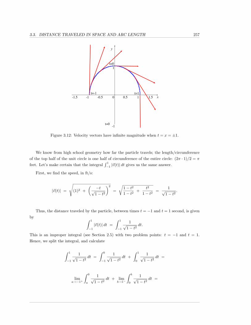
3.3. DISTANCE TRAVELED IN SPACE AND ARC LENGTH 257
-1.5 -1 -0.5 0 0.5 1 1.5
-1
1
t=-1
t=0
t=1
t=0
Figure 3.12: Velocity vectors have infinite magnitude when t = x = ±1.
We know from high school geometry how far the particle travels; the length/circumferenceof the top half of the unit circle is one half of circumference of the entire circle: (2π · 1)/2 = π
feet. Let’s make certain that the integral∫ 1
−1|~v(t)| dt gives us the same answer.
First, we find the speed, in ft/s:
|~v(t)| =
√(1)2 +
(−t√
1− t2
)2
=
√1− t21− t2
+t2
1− t2=
1√1− t2
.
Thus, the distance traveled by the particle, between times t = −1 and t = 1 second, is givenby ∫ 1
−1
|~v(t)| dt =∫ 1
−1
1√1− t2
dt.
This is an improper integral (see Section 2.5) with two problem points: t = −1 and t = 1.Hence, we split the integral, and calculate
∫ 1
−1
1√1− t2
dt =∫ 0
−1
1√1− t2
dt +∫ 1
0
1√1− t2
dt =
lima→−1+
∫ 0
a
1√1− t2
dt + limb→1−
∫ b
0
1√1− t2
dt =
258 CHAPTER 3. APPLICATIONS OF INTEGRATION
lima→−1+
(sin−1 t
∣∣∣0a
)+ lim
b→1−
(sin−1 t
∣∣∣b0
)=(0− lim
a→−1+sin−1 a
)+(
limb→1−
sin−1 b− 0)
=
−(−π
2
)+π
2= π feet.
Whew! It sure took a while to verify that the length of a semicircle of radius 1 is π.
Arc length:
The term length in this context is usually augmented and is referred to as arc length, inorder to emphasize that we mean the length along something which curves (i.e., along somethingwhich is composed of “arcs”).
Example 3.3.8. If all we want is to use integration to verify that the arc length of a semicircleof radius 1 is equal to π, perhaps it would be better to think of a particle which moves aroundthe semicircle at a different speed from that of the particle in Example 3.3.7.
Suppose that a particle moves in the xy-plane in such a way that its position ~p(t), in feet,at time t seconds, where 0 ≤ t ≤ π, is given by
~p(t) = (− cos t, sin t).
Then, we see that the x- and y-coordinates of the particle are given by x = − cos t and y = sin t,so that x2 +y2 = (− cos t)2 +sin2 t = 1. Hence, once again, the particle is always on the circle ofradius 1, centered at the origin. We also see that y = sin t ≥ 0 for 0 ≤ t ≤ π, that ~p(0) = (−1, 0),and that ~p(π) = (1, 0). Finally, it is important to note that ~p(t) is one-to-one, i.e., the particleis never at the same point at two (or more) different times.
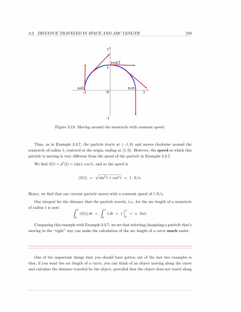
3.3. DISTANCE TRAVELED IN SPACE AND ARC LENGTH 259
-1 0 1
-1
1
t=0
t=π/2
t=π
Figure 3.13: Moving around the semicircle with constant speed.
Thus, as in Example 3.3.7, the particle starts at (−1, 0) and moves clockwise around thesemicircle of radius 1, centered at the origin, ending at (1, 0). However, the speed at which thisparticle is moving is very different from the speed of the particle in Example 3.3.7.
We find ~v(t) = ~p ′(t) = (sin t, cos t), and so the speed is
|~v(t)| =√
sin2 t+ cos2 t = 1 ft/s.
Hence, we find that our current particle moves with a constant speed of 1 ft/s.
Our integral for the distance that the particle travels, i.e., for the arc length of a semicircleof radius 1 is now: ∫ π
0
|~v(t)| dt =∫ π
0
1 dt = t∣∣∣π0
= π feet.
Comparing this example with Example 3.3.7, we see that selecting/imagining a particle that’smoving in the “right” way can make the calculation of the arc length of a curve much easier.
One of the important things that you should have gotten out of the last two examples isthat, if you want the arc length of a curve, you can think of an object moving along the curveand calculate the distance traveled by the object, provided that the object does not travel along
260 CHAPTER 3. APPLICATIONS OF INTEGRATION
any portions of the curve more than once; this means that the position function should be one-to-one. We also saw that the calculation of the distance traveled can be made much easier bymaking a nice choice of a position function.
In fact, it doesn’t matter whether or not we actually think of an object moving along a givencurve. What’s important is that we have a one-to-one, continuously differentiable function ~p(t)from a closed interval [a, b], where a < b, into the xy-plane or into xyz-space, that plays therole of a position function, in that the points on the curve that we’re interested in are preciselythe points that you get from ~p(t), i.e., the curve whose arc length we want is the range of thefunction ~p. The term simple is frequently used in this context to indicate that ~p is one-to-one.
We also require, for now, a condition, regularity, which, in terms of motion, would say thatthe object never stops at times in the open interval (a, b); this technical condition is very usefulmathematically.
Definition 3.3.9. A simple regular parameterization of a curve in Rn (e.g., in R2,the xy-plane, or in R3, xyz-space) is a one-to-one, continuously differentiable function ~pfrom a closed interval [a, b], where a < b, into Rn, such that, for all t in [a, b], ~p ′(t) 6= ~0.
The range of a simple regular parameterization, that is, the set of points that ~p(t) “passesthrough”, is called a simple regular curve.
We say that a simple regular parameterization ~p, with domain [a, b], parameterizes thesimple regular curve which is its range, and that the parameterization starts at the point~p(a) and ends at the point ~p(b).
Remark 3.3.10. We have defined a simple regular curve C as a set of points in R2 or R3,and you should have an intuitive idea of what a curve looks like, but how can we rigorously,mathematically, say when a set of points matches your intuition for what a curve is?
What we have said in Definition 3.3.9 is that a rigorous definition of a simple regular curve isthat it is the range of a simple regular parametrization; but keep in mind that, as we saw in theprevious two examples, a simple regular curve, like a semicircle, can have more than one simpleregular parameterization. In fact, it is not difficult to show that any simple regular curve hasan infinite number of different simple regular parameterizations. Nonetheless, as we saw in theprevious two examples, the curve itself has a length which is independent of the simple regularparameterization, i.e.,
∫ ba|~p ′(t)| dt will give the same number, regardless of what simple regular
parameterization you use for a given simple regular curve.
3.3. DISTANCE TRAVELED IN SPACE AND ARC LENGTH 261
Finally, we should mention that, in many references, a curve is defined to be the param-eterization ~p, not the range of this function. This is mathematically convenient, but doesnot agree with most people’s intuition for what a “curve” is, and so we will not use theterminology.
What we have seen in our discussion and examples is that an infinitesimal piece of arc length,ds is equal to |~p ′(t)| dt, and so we have:
Proposition 3.3.11. Suppose that C is a simple regular curve in R2 or in R3. Then, forany simple regular parameterization ~p(t), with domain [a, b], of C, the arc length of C is
∫ t=b
t=a
ds =∫ b
a
|~p ′(t)| dt.
Curves in the plane:
In our next examples of arc length calculations, we are going to look at simple regular curvesin R2, the xy-plane. In the plane, there are three common ways to specify simple regularparameterizations.
One way is to specify appropriate coordinate (or component) functions x = x(t) and y = y(t),and then the parameterization is, of course, ~p(t) = (x(t), y(t)). Then, Proposition 3.3.11 tellsus:
Proposition 3.3.12. If ~p(t) = (x(t), y(t)), for a ≤ t ≤ b, is a simple regular parameteriza-tion of a curve C in R2, then
ds =
√(dx
dt
)2
+(dy
dt
)2
dt,
and
arc length of C =∫ b
a
√(dx
dt
)2
+(dy
dt
)2
dt.
262 CHAPTER 3. APPLICATIONS OF INTEGRATION
However, you are probably most familiar with curves described as the graph of y = f(x),where a ≤ x ≤ b, and where f is continuously differentiable. There is an obvious parame-terization here: x = t and y = f(t), i.e., ~p(t) = (t, f(t)). This ~p is clearly one-to-one, since(t1, f(t1)) = (t2, f(t2)) immediately implies that t1 = t2. In addition, using that t = x, we have
√(dx
dt
)2
+(dy
dt
)2
=
√(dx
dx
)2
+(df
dx
)2
=
√1 +
(df
dx
)2
> 0.
Therefore, if f is continuously differentiable on an open interval containing [a, b], then ~p(t) =(t, f(t)) is a simple regular parameterization.
Proposition 3.3.13. If y = f(x) is continuously differentiable on an open interval con-taining [a, b], then
ds =
√1 +
(dy
dx
)2
dx
and the arc length of the graph of f , for a ≤ x ≤ b, is
∫ b
a
√1 +
(dy
dx
)2
dx.
While it’s less common, a curve may also be described by specifying x as a function of y,instead of giving y as a function of x. Of course, all this does is interchange the roles of x andy.
Proposition 3.3.14. If x = f(y) is continuously differentiable on an open interval con-taining [a, b], then
ds =
√1 +
(dx
dy
)2
dy,
and the arc length of the graph of f , for a ≤ y ≤ b, is
∫ b
a
√1 +
(dx
dy
)2
dy.
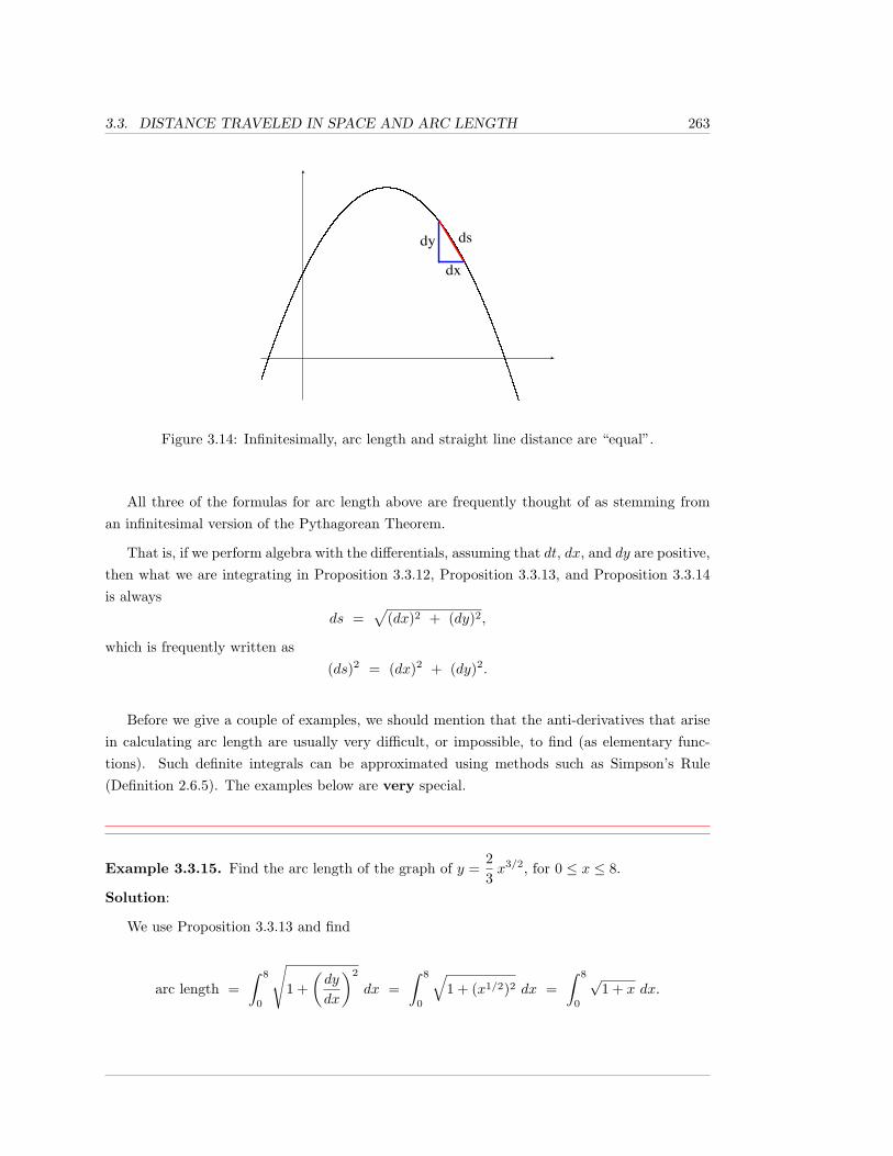
3.3. DISTANCE TRAVELED IN SPACE AND ARC LENGTH 263
dx
dy ds
Figure 3.14: Infinitesimally, arc length and straight line distance are “equal”.
All three of the formulas for arc length above are frequently thought of as stemming froman infinitesimal version of the Pythagorean Theorem.
That is, if we perform algebra with the differentials, assuming that dt, dx, and dy are positive,then what we are integrating in Proposition 3.3.12, Proposition 3.3.13, and Proposition 3.3.14is always
ds =√
(dx)2 + (dy)2,
which is frequently written as(ds)2 = (dx)2 + (dy)2.
Before we give a couple of examples, we should mention that the anti-derivatives that arisein calculating arc length are usually very difficult, or impossible, to find (as elementary func-tions). Such definite integrals can be approximated using methods such as Simpson’s Rule(Definition 2.6.5). The examples below are very special.
Example 3.3.15. Find the arc length of the graph of y =23x3/2, for 0 ≤ x ≤ 8.
Solution:
We use Proposition 3.3.13 and find
arc length =∫ 8
0
√1 +
(dy
dx
)2
dx =∫ 8
0
√1 + (x1/2)2 dx =
∫ 8
0
√1 + x dx.
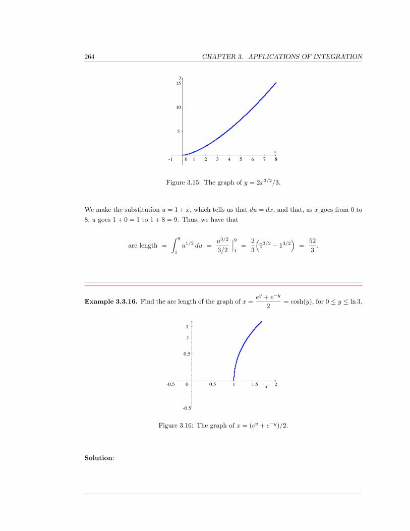
264 CHAPTER 3. APPLICATIONS OF INTEGRATION
-1 0 1 2 3 4 5 6 7 8
5
10
15
Figure 3.15: The graph of y = 2x3/2/3.
We make the substitution u = 1 + x, which tells us that du = dx, and that, as x goes from 0 to8, u goes 1 + 0 = 1 to 1 + 8 = 9. Thus, we have that
arc length =∫ 9
1
u1/2 du =u3/2
3/2
∣∣∣91
=23
(93/2 − 13/2
)=
523.
Example 3.3.16. Find the arc length of the graph of x =ey + e−y
2= cosh(y), for 0 ≤ y ≤ ln 3.
-0.5 0 0.5 1 1.5 2
-0.5
0.5
1
Figure 3.16: The graph of x = (ey + e−y)/2.
Solution:
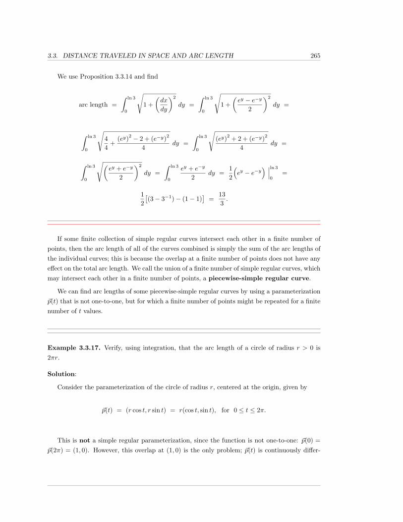
3.3. DISTANCE TRAVELED IN SPACE AND ARC LENGTH 265
We use Proposition 3.3.14 and find
arc length =∫ ln 3
0
√1 +
(dx
dy
)2
dy =∫ ln 3
0
√1 +
(ey − e−y
2
)2
dy =
∫ ln 3
0
√44
+(ey)2 − 2 + (e−y)2
4dy =
∫ ln 3
0
√(ey)2 + 2 + (e−y)2
4dy =
∫ ln 3
0
√(ey + e−y
2
)2
dy =∫ ln 3
0
ey + e−y
2dy =
12
(ey − e−y
) ∣∣∣ln 3
0=
12[(3− 3−1)− (1− 1)
]=
133.
If some finite collection of simple regular curves intersect each other in a finite number ofpoints, then the arc length of all of the curves combined is simply the sum of the arc lengths ofthe individual curves; this is because the overlap at a finite number of points does not have anyeffect on the total arc length. We call the union of a finite number of simple regular curves, whichmay intersect each other in a finite number of points, a piecewise-simple regular curve.
We can find arc lengths of some piecewise-simple regular curves by using a parameterization~p(t) that is not one-to-one, but for which a finite number of points might be repeated for a finitenumber of t values.
Example 3.3.17. Verify, using integration, that the arc length of a circle of radius r > 0 is2πr.
Solution:
Consider the parameterization of the circle of radius r, centered at the origin, given by
~p(t) = (r cos t, r sin t) = r(cos t, sin t), for 0 ≤ t ≤ 2π.
This is not a simple regular parameterization, since the function is not one-to-one: ~p(0) =~p(2π) = (1, 0). However, this overlap at (1, 0) is the only problem; ~p(t) is continuously differ-
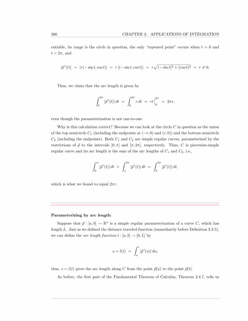
266 CHAPTER 3. APPLICATIONS OF INTEGRATION
entiable, its range is the circle in question, the only “repeated point” occurs when t = 0 andt = 2π, and
|~p ′(t)| = |r(− sin t, cos t)| = r |(− sin t, cos t)| = r√
(− sin t)2 + (cos t)2 = r 6= 0.
Thus, we claim that the arc length is given by
∫ 2π
0
|~p ′(t)| dt =∫ 2π
0
r dt = rt∣∣∣2π0
= 2πr,
even though the parameterization is not one-to-one.
Why is this calculation correct? Because we can look at the circle C in question as the unionof the top semicircle C1 (including the endpoints at (−r, 0) and (r, 0)) and the bottom semicircleC2 (including the endpoints). Both C1 and C2 are simple regular curves, parameterized by therestrictions of ~p to the intervals [0, π] and [π, 2π], respectively. Thus, C is piecewise-simpleregular curve and its arc length is the sum of the arc lengths of C1 and C2, i.e.,
∫ π
0
|~p ′(t)| dt +∫ 2π
π
|~p ′(t)| dt =∫ 2π
0
|~p ′(t)| dt,
which is what we found to equal 2πr.
Parameterizing by arc length:
Suppose that ~p : [a, b] → Rn is a simple regular parameterization of a curve C, which haslength L. Just as we defined the distance traveled function (immediately before Definition 3.3.5),we can define the arc length function l : [a, b]→ [0, L] by
s = l(t) =∫ t
a
|~p ′(u)| du;
thus, s = l(t) gives the arc length along C from the point ~p(a) to the point ~p(t).
As before, the first part of the Fundamental Theorem of Calculus, Theorem 2.4.7, tells us
3.3. DISTANCE TRAVELED IN SPACE AND ARC LENGTH 267
thatl′(t) =
ds
dt= |~p ′(t)|.
As ~p is a regular parameterization, |~p ′(t)| > 0, and so the Inverse Function Theorem implies thatl has a monotonically increasing, differentiable inverse function, i.e., there exists a differentiablefunction t = m(s) such that m(0) = a, m(L) = b, and l(m(s)) = s, for all s in the interval[0, L], and m(l(t)) = t, for all t in the interval [a, b]. From the Chain Rule (or the formula forthe derivative of an inverse function), we have that
m′(s) =1
l′(m(s))=
1|~p ′(m(s))|
It is easy to check that the composed function ~q = ~p ◦ m : [0, L] → Rn is again a simpleregular parameterization of C, and has the property that ~q(s) is the unique point on the curveC which is distance (along C) s away from ~q(0) = ~p(a).
Definition 3.3.18. A parameterization such as ~q, where the parameter measures arc lengthalong C, is said to be a parameterization by arc length.
Note that if ~q : [0, L]→ Rn is a simple regular parameterization, parameterized by arc length,then, applying the Chain Rule (to each component of the vector), we find
|~q ′(s)| = |(~p ◦m) ′(s)| = |m′(s)~p ′(m(s))| = |m′(s)| |~p ′(m(s))| =
1|~p ′(m(s))|
· |~p ′(m(s))| = 1.
This, of course, gives us what it had better give us: if we use ~q to define the arc lengthfunction, we get ∫ s
0
|~q ′(u)| du =∫ s
0
1 du = u∣∣∣s0
= s,
which, in words, says that if you calculate the arc length between the starting point of a (pa-rameterized) simple regular curve and the point that’s the distance s away (along C) from thestarting point, then what you get is s. If that sounds stupidly obvious, GOOD.
One final remark on parameterizing by arc length: if we return to the situation of an objectmoving along a curve, with a simple regular position function ~p = ~p(t), where t is time, thenthe parameter t is also the arc length (so that ~p(t) is a parameterization by arc length) if and
268 CHAPTER 3. APPLICATIONS OF INTEGRATION
only if, for all t, |~p ′(t)| = 1. Thus, a parameterization by arc length is also referred to as aparameterization with unit speed, or speed 1.
More general parameterized curves:
If we combine parameterizations like those in Example 3.3.7 and in Example 3.3.17, we findthat we can deal with curves that are the ranges of parameterizations which may fail to satisfyvarious conditions at a finite number of points. We don’t need for our parameterizations to haveclosed intervals as their domains. We also don’t require that ~p is continuously differentiableeverywhere, and so ~p ′ need not be defined at some points, and even the improper integral (recallSection 2.5) of |~p ′(t)| is not automatically guaranteed to exist.
All of these things make the definition below very technical. You need to recall our mostgeneral notion of integrating over fairly general sets of points from Definition 2.5.11. The term“rectifiable”, used below, is a technical term which implies that a reasonable notion of arc lengthexists for the curve in question.
Definition 3.3.19. A rectifiable parameterization of a curve in Rn is a continuousfunction ~p from an interval I, whose interior is non-empty, into Rn, such that there exists afinite set of points F (which could be empty) in I such that, the restriction of ~p to the pointsof I which are not in F (i.e., to the set I−F ) is one-to-one, continuously differentiable, hasan everywhere non-zero derivative, and such that the (possibly) improper integral
∫I|~p ′(t)| dt
exists.
The range of a rectifiable parameterization is a rectifiable, piecewise-regular, curve.
Of course, we have:
Proposition 3.3.20. Suppose that C is a rectifiable, piecewise-regular, curve. Then, forany rectifiable parameterization ~p(t), with domain I, of C, the arc length of C is
∫I
|~p ′(t)| dt.
3.3. DISTANCE TRAVELED IN SPACE AND ARC LENGTH 269
3.3.1 Exercises
You are given the velocity function ~v(t) of a object in Exercises 1 - 6. Calculate the
displacement of the object over the given time interval.
1. ~v(t) = (3 sin 2πt, 3 cos 2πt, 4t), [0, 2].
2. ~v(t) = (t2 + t, 4t3, 0), [0, 3].
3. ~v(t) = (3 + 4t, 5− 7t, 11t), [−3, 7].
4. ~v(t) = (−15, t+ 4, sinh t), [−5, 8].
5. ~v(t) = (|t|, |t|, |t|), [−3, 3].
6. ~v(t) = (t ln t, 1/t, e−t), [1, 5].
Say whether the given map is a simple regular parameterization of a curve. If it’s
not, say why it is not.
7. ~λ(t) = (2t3, 16, cos t), t ∈ [−10, 10].
8. ~α(t) = (cos t, |t+ 2|, sin t), t ∈ [−π, 0].
9. ~u(t) = (cos t, |t+ 2|, sin t), t ∈ [0, π].
10. ~w(t) = (1, t, t2), t ∈ [−12, 20].
11. ~h(t) = (t3, t3, t3), t ∈ [−5, 5].
In each of Exercises 12 through 14, give an arc length parameterization of the given
curve.
12. ~α(t) = (cos 5t, sin 5t), t ∈ [0, 2π/5].
13. ~w(t) = (3 + 6t, 2− 5t, 7 + t), t ∈ [0, 4].
14. ~z(t) = (t3/3, 0, t+ 3), t ∈ [1, 3].
15. Suppose φ : [a, b] → Rn is a regular curve parameterized by arc length. Show that thelength of the curve is b− a.
16. A regular α : [a, b] → Rn is closed if α(a) = α(b). Note that α must still be one-to-oneeverywhere else.
270 CHAPTER 3. APPLICATIONS OF INTEGRATION
a. If α is a closed regular position function, show that the total displacement over theinterval is ~0.
b. Give a simple example that shows that while the displacement is zero, the totaldistance traveled may be non-zero.
You are given the position function of a particle. Calculate the total distance
traveled by the particle over the given time interval.
17. ~p(t) = (−t, t, 3), t ∈ [0, π/4].
18. ~p(t) = (t, 12, 0.5e2t), t ∈ [0, 1].
19. ~p(t) = (sin 3t, cos 3t, 2t3/2), t ∈ [0, π].
Calculate the arc length of the graph of the function over the interval I.
20. f(x) = ax+ b, a 6= 0, I = [c, d].
21. g(x) = ln(sinx), I = [π/4, π/2].
22. f(y) = eay, a > 0, I = [0, 1].
23. h(y) = 5 ln y, I = [1, 5].
24. f(x) =x3
12+
1x
. I = [1, 2].
25. Generalize the previous problem. Let a > 0 and f(x) =x3
6√a
+√a
2x, I = [1, 2] and calculate
the arc length of the graph.
26. Suppose ~p(t) = (a cos t, a sin t, b cos t, b sin t), t ∈ [0, 2π] is the position function of a particle
traveling in R4. What is the total distance traveled?
27. Parameterize the curve in the previous example by arc length.
28. What is the image of the curve (t3, t3), t ∈ R? Is this curve regular?
29. Is the path (t, |t|) regular? Is it rectifiable on the in the interval [−1, 1]?
30. The intersection of a sphere centered at the origin with radius R and the plane z =z0, −R < z0 < R is a circle. Give a parameterization of this circle and calculate itscircumference in terms of z0 and R.
31. Suppose you make a journey (on the Earth) consisting of three legs. Assume the Earth isa sphere centered at the origin with radius R. You start at the North Pole and travel to apoint on the equator along a line of longitude. You then walk along the equator through90 degrees of longitude. Finally, you travel back along the equator.
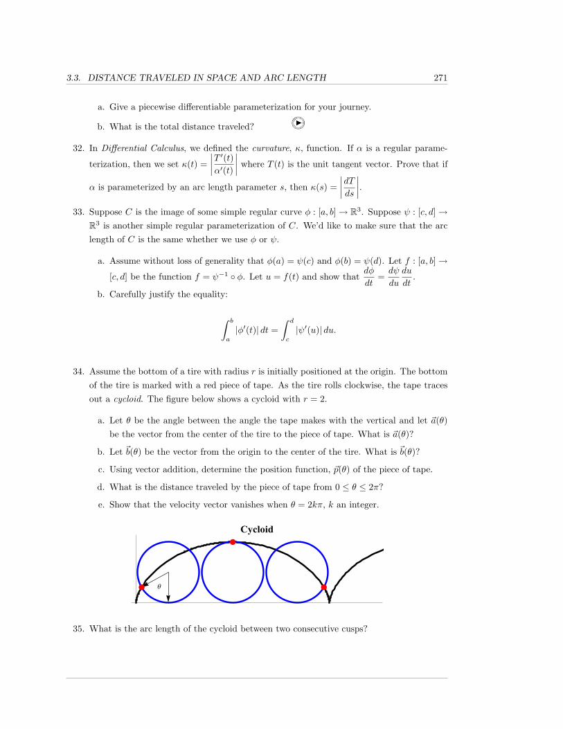
3.3. DISTANCE TRAVELED IN SPACE AND ARC LENGTH 271
a. Give a piecewise differentiable parameterization for your journey.
b. What is the total distance traveled?
32. In Differential Calculus, we defined the curvature, κ, function. If α is a regular parame-
terization, then we set κ(t) =∣∣∣∣T ′(t)α′(t)
∣∣∣∣ where T (t) is the unit tangent vector. Prove that if
α is parameterized by an arc length parameter s, then κ(s) =∣∣∣∣dTds
∣∣∣∣.33. Suppose C is the image of some simple regular curve φ : [a, b]→ R3. Suppose ψ : [c, d]→
R3 is another simple regular parameterization of C. We’d like to make sure that the arclength of C is the same whether we use φ or ψ.
a. Assume without loss of generality that φ(a) = ψ(c) and φ(b) = ψ(d). Let f : [a, b]→
[c, d] be the function f = ψ−1 ◦ φ. Let u = f(t) and show thatdφ
dt=dψ
du
du
dt.
b. Carefully justify the equality:
∫ b
a
|φ′(t)| dt =∫ d
c
|ψ′(u)| du.
34. Assume the bottom of a tire with radius r is initially positioned at the origin. The bottomof the tire is marked with a red piece of tape. As the tire rolls clockwise, the tape tracesout a cycloid. The figure below shows a cycloid with r = 2.
a. Let θ be the angle between the angle the tape makes with the vertical and let ~a(θ)be the vector from the center of the tire to the piece of tape. What is ~a(θ)?
b. Let ~b(θ) be the vector from the origin to the center of the tire. What is ~b(θ)?
c. Using vector addition, determine the position function, ~p(θ) of the piece of tape.
d. What is the distance traveled by the piece of tape from 0 ≤ θ ≤ 2π?
e. Show that the velocity vector vanishes when θ = 2kπ, k an integer.
Θ
Cycloid
35. What is the arc length of the cycloid between two consecutive cusps?
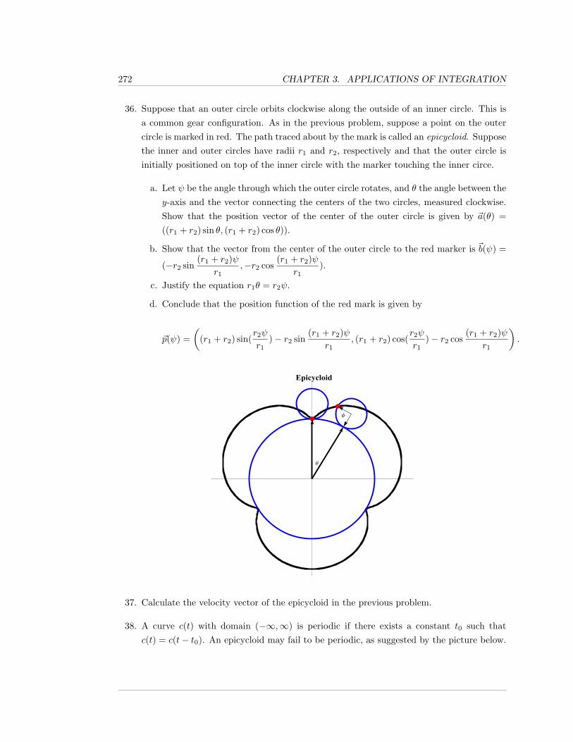
272 CHAPTER 3. APPLICATIONS OF INTEGRATION
36. Suppose that an outer circle orbits clockwise along the outside of an inner circle. This isa common gear configuration. As in the previous problem, suppose a point on the outercircle is marked in red. The path traced about by the mark is called an epicycloid. Supposethe inner and outer circles have radii r1 and r2, respectively and that the outer circle isinitially positioned on top of the inner circle with the marker touching the inner circe.
a. Let ψ be the angle through which the outer circle rotates, and θ the angle between they-axis and the vector connecting the centers of the two circles, measured clockwise.Show that the position vector of the center of the outer circle is given by ~a(θ) =((r1 + r2) sin θ, (r1 + r2) cos θ)).
b. Show that the vector from the center of the outer circle to the red marker is ~b(ψ) =
(−r2 sin(r1 + r2)ψ
r1,−r2 cos
(r1 + r2)ψr1
).
c. Justify the equation r1θ = r2ψ.
d. Conclude that the position function of the red mark is given by
~p(ψ) =(
(r1 + r2) sin(r2ψ
r1)− r2 sin
(r1 + r2)ψr1
, (r1 + r2) cos(r2ψ
r1)− r2 cos
(r1 + r2)ψr1
).
Ψ
Θ
Epicycloid
37. Calculate the velocity vector of the epicycloid in the previous problem.
38. A curve c(t) with domain (−∞,∞) is periodic if there exists a constant t0 such thatc(t) = c(t− t0). An epicycloid may fail to be periodic, as suggested by the picture below.
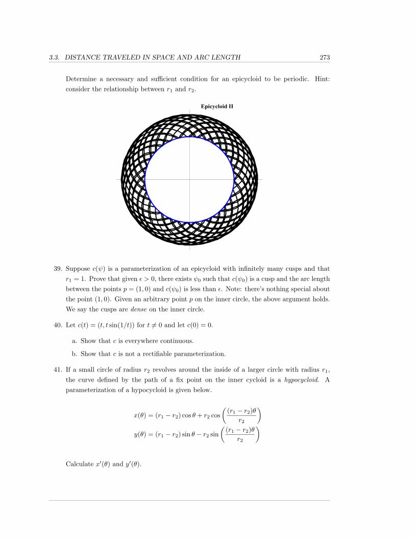
3.3. DISTANCE TRAVELED IN SPACE AND ARC LENGTH 273
Determine a necessary and sufficient condition for an epicycloid to be periodic. Hint:consider the relationship between r1 and r2.
Epicycloid II
39. Suppose c(ψ) is a parameterization of an epicycloid with infinitely many cusps and thatr1 = 1. Prove that given ε > 0, there exists ψ0 such that c(ψ0) is a cusp and the arc lengthbetween the points p = (1, 0) and c(ψ0) is less than ε. Note: there’s nothing special aboutthe point (1, 0). Given an arbitrary point p on the inner circle, the above argument holds.We say the cusps are dense on the inner circle.
40. Let c(t) = (t, t sin(1/t)) for t 6= 0 and let c(0) = 0.
a. Show that c is everywhere continuous.
b. Show that c is not a rectifiable parameterization.
41. If a small circle of radius r2 revolves around the inside of a larger circle with radius r1,the curve defined by the path of a fix point on the inner cycloid is a hypocycloid. Aparameterization of a hypocycloid is given below.
x(θ) = (r1 − r2) cos θ + r2 cos(
(r1 − r2)θr2
)y(θ) = (r1 − r2) sin θ − r2 sin
((r1 − r2)θ
r2
)
Calculate x′(θ) and y′(θ).
274 CHAPTER 3. APPLICATIONS OF INTEGRATION
42. Show that in a hypocycloid where the ratio of r1 to r2 is 4 to 1, the coordinates satisfyx2/3 + y2/3 = C, where C is some constant.
43. Students not familiar with the dot product should skip this problem. Supposep and q are two distinct points in R3. We’d like to confirm our intuition that the straightline segment connecting these two points is the shortest curve among those with endpointsp and q. More precisely, we’ll show that any curve between these two points must be atleast as long as the straight line segment between them.
a. Let ~c : [a, b] → R3 be any simple regular curve such that c(a) = p and c(b) = q. Let~v be any unit vector (so, |~v| = 1). Prove that (q − p) · ~v =
∫ ba~c ′(t) · ~v dt.
b. Prove that∫ ba~c ′(t) · ~v dt ≤
∫ ba|~c ′(t)| dt. Hint: one way to do this is to use the fact
that ~x · ~y = |~x||~y| cos θ.
c. Let v =p− q|p− q|
and conclude that
|p− q| ≤∫ b
a
|~c′(t)| dt.
In other words, the length of an arbitrary curve from p to q is at least as long as thestraight line segment between p and q.
44. A curve may be parametrized for unbounded time, and yet still have finite length. Let~p(t) = (ae−bt cos t, ae−bt sin t) where a, b > 0 and t ∈ R. The image of this parameteriza-tion is called the logarithmic spiral.
a. Calculate |~p ′(t)|.
b. What is limt→∞
∫ t
0
|~p ′(u)| du?
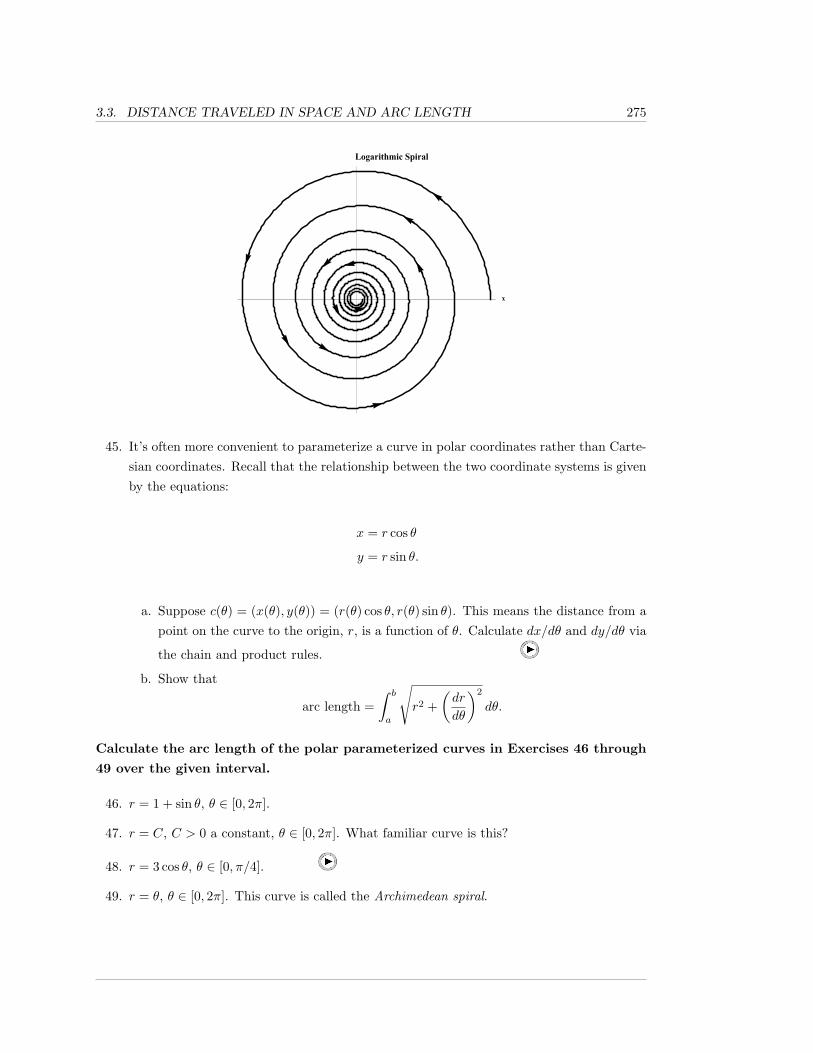
3.3. DISTANCE TRAVELED IN SPACE AND ARC LENGTH 275
x
Logarithmic Spiral
45. It’s often more convenient to parameterize a curve in polar coordinates rather than Carte-sian coordinates. Recall that the relationship between the two coordinate systems is givenby the equations:
x = r cos θ
y = r sin θ.
a. Suppose c(θ) = (x(θ), y(θ)) = (r(θ) cos θ, r(θ) sin θ). This means the distance from apoint on the curve to the origin, r, is a function of θ. Calculate dx/dθ and dy/dθ via
the chain and product rules.
b. Show that
arc length =∫ b
a
√r2 +
(dr
dθ
)2
dθ.
Calculate the arc length of the polar parameterized curves in Exercises 46 through
49 over the given interval.
46. r = 1 + sin θ, θ ∈ [0, 2π].
47. r = C, C > 0 a constant, θ ∈ [0, 2π]. What familiar curve is this?
48. r = 3 cos θ, θ ∈ [0, π/4].
49. r = θ, θ ∈ [0, 2π]. This curve is called the Archimedean spiral.
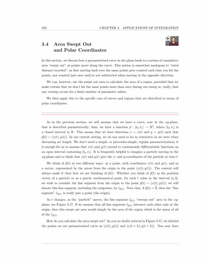
276 CHAPTER 3. APPLICATIONS OF INTEGRATION
3.4 Area Swept Outand Polar Coordinates
In this section, we discuss how a parameterized curve in the plane leads to a notion of cumulativearea “swept out” as points move along the curve. This notion is somewhat analogous to “totaldistance traveled”, in that moving back over the same points gets counted each time you hit thepoints, not counted just once and/or not subtracted when moving in the opposite direction.
We can, however, use the swept out area to calculate the area of a region, provided that wemake certain that we don’t hit the same points more than once during our sweep or, really, thatany overlap occurs for a finite number of parameter values.
We then apply this to the specific case of curves and regions that are described in terms ofpolar coordinates.
As in the previous section, we will assume that we have a curve, now in the xy-plane,that is described parametrically; thus, we have a function ~p : [t0, t1] → R2, where [t0, t1] isa closed interval in R. This means that we have functions x = x(t) and y = y(t) such that~p(t) = (x(t), y(t)). In our current setting, we do not need to be as restrictive as we were whendiscussing arc length. We don’t need a simple, or piecewise-simple, regular parameterization; itis enough for us to assume that x(t) and y(t) extend to continuously differentiable functions onan open interval containing [t0, t1]. It is frequently helpful to imagine a particle moving in thexy-plane and to think that x(t) and y(t) give the x- and y-coordinates of the particle at time t.
We think of ~p(t) in two different ways: as a point, with coordinates x(t) and y(t), and asa vector, represented by the arrow from the origin to the point (x(t), y(t)). The context willalways make it clear how we are thinking of ~p(t). Whether you think of ~p(t) as the positionvector of a particle or as a purely mathematical point, for each t value in the interval [a, b],we wish to consider the line segment from the origin to the point ~p(t) = (x(t), y(t)); we willdenote this line segment, including the endpoints, by `~p(t). Note that, if ~p(t) = ~0, then the “linesegment” `~p(t) is really just a point (the origin).
As t changes, as the “particle” moves, the line segment `~p(t) “sweeps out” area in the xy-plane; see Figure 3.17. If we assume that all line segments `~p(t) intersect each other only at theorigin, then this swept out area would simply be the area of the region which is the union of allof the `~p(t).
How do you calculate the area swept out? As you no doubt noticed in Figure 3.17, we labeledthe points on our parameterized curve as (x(t), y(t)) and (x(t + h), y(t + h)). You may have
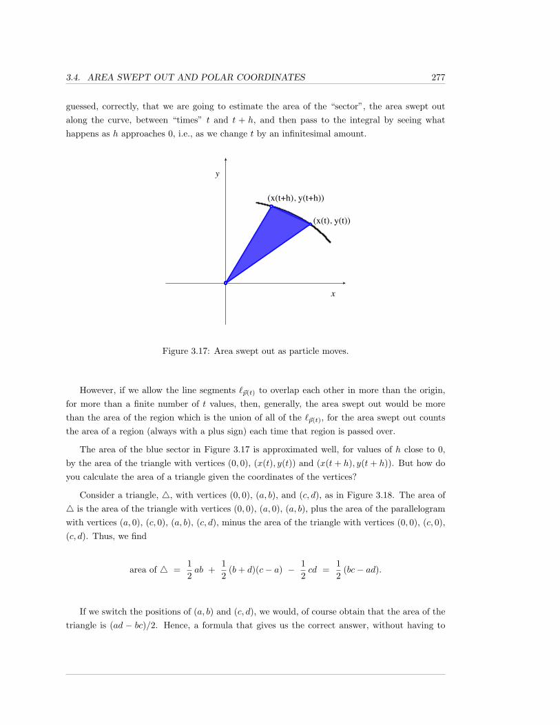
3.4. AREA SWEPT OUT AND POLAR COORDINATES 277
guessed, correctly, that we are going to estimate the area of the “sector”, the area swept outalong the curve, between “times” t and t + h, and then pass to the integral by seeing whathappens as h approaches 0, i.e., as we change t by an infinitesimal amount.
(x(t), y(t))
(x(t+h), y(t+h))
Figure 3.17: Area swept out as particle moves.
However, if we allow the line segments `~p(t) to overlap each other in more than the origin,for more than a finite number of t values, then, generally, the area swept out would be morethan the area of the region which is the union of all of the `~p(t), for the area swept out countsthe area of a region (always with a plus sign) each time that region is passed over.
The area of the blue sector in Figure 3.17 is approximated well, for values of h close to 0,by the area of the triangle with vertices (0, 0), (x(t), y(t)) and (x(t+ h), y(t+ h)). But how doyou calculate the area of a triangle given the coordinates of the vertices?
Consider a triangle, 4, with vertices (0, 0), (a, b), and (c, d), as in Figure 3.18. The area of4 is the area of the triangle with vertices (0, 0), (a, 0), (a, b), plus the area of the parallelogramwith vertices (a, 0), (c, 0), (a, b), (c, d), minus the area of the triangle with vertices (0, 0), (c, 0),(c, d). Thus, we find
area of 4 =12ab +
12
(b+ d)(c− a) − 12cd =
12
(bc− ad).
If we switch the positions of (a, b) and (c, d), we would, of course obtain that the area of thetriangle is (ad − bc)/2. Hence, a formula that gives us the correct answer, without having to
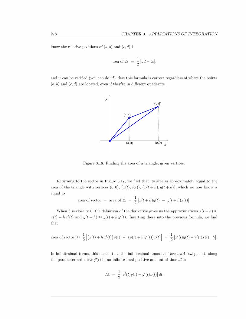
278 CHAPTER 3. APPLICATIONS OF INTEGRATION
know the relative positions of (a, b) and (c, d) is
area of 4 =12
∣∣ad− bc∣∣,and it can be verified (you can do it!) that this formula is correct regardless of where the points(a, b) and (c, d) are located, even if they’re in different quadrants.
(a,b)
(c,d)
(c,0)(a,0)
Figure 3.18: Finding the area of a triangle, given vertices.
Returning to the sector in Figure 3.17, we find that its area is approximately equal to thearea of the triangle with vertices (0, 0), (x(t), y(t)), (x(t + h), y(t + h)), which we now know isequal to
area of sector = area of 4 =12
∣∣x(t+ h)y(t) − y(t+ h)x(t)∣∣.
When h is close to 0, the definition of the derivative gives us the approximations x(t+ h) ≈x(t) + hx′(t) and y(t + h) ≈ y(t) + h y′(t). Inserting these into the previous formula, we findthat
area of sector ≈ 12
∣∣∣(x(t) + hx′(t))y(t) −
(y(t) + h y′(t)
)x(t)
∣∣∣ =12
∣∣x′(t)y(t)− y′(t)x(t)∣∣ ∣∣h∣∣.
In infinitesimal terms, this means that the infinitesimal amount of area, dA, swept out, alongthe parameterized curve ~p(t) in an infinitesimal positive amount of time dt is
dA =12
∣∣x′(t)y(t)− y′(t)x(t)∣∣ dt.
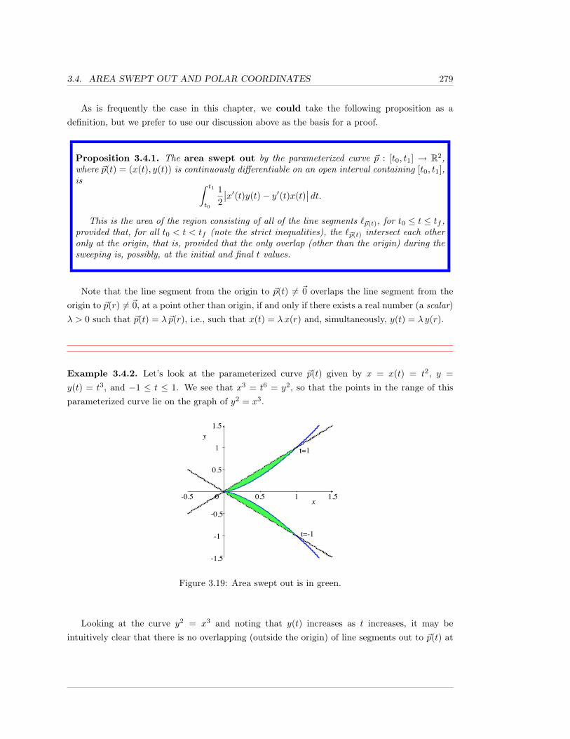
3.4. AREA SWEPT OUT AND POLAR COORDINATES 279
As is frequently the case in this chapter, we could take the following proposition as adefinition, but we prefer to use our discussion above as the basis for a proof.
Proposition 3.4.1. The area swept out by the parameterized curve ~p : [t0, t1] → R2,where ~p(t) = (x(t), y(t)) is continuously differentiable on an open interval containing [t0, t1],is ∫ t1
t0
12
∣∣x′(t)y(t)− y′(t)x(t)∣∣ dt.
This is the area of the region consisting of all of the line segments `~p(t), for t0 ≤ t ≤ tf ,provided that, for all t0 < t < tf (note the strict inequalities), the `~p(t) intersect each otheronly at the origin, that is, provided that the only overlap (other than the origin) during thesweeping is, possibly, at the initial and final t values.
Note that the line segment from the origin to ~p(t) 6= ~0 overlaps the line segment from theorigin to ~p(r) 6= ~0, at a point other than origin, if and only if there exists a real number (a scalar)λ > 0 such that ~p(t) = λ ~p(r), i.e., such that x(t) = λx(r) and, simultaneously, y(t) = λ y(r).
Example 3.4.2. Let’s look at the parameterized curve ~p(t) given by x = x(t) = t2, y =y(t) = t3, and −1 ≤ t ≤ 1. We see that x3 = t6 = y2, so that the points in the range of thisparameterized curve lie on the graph of y2 = x3.
-0.5 0 0.5 1 1.5
-1.5
-1
-0.5
0.5
1
1.5
t=-1
t=1
Figure 3.19: Area swept out is in green.
Looking at the curve y2 = x3 and noting that y(t) increases as t increases, it may beintuitively clear that there is no overlapping (outside the origin) of line segments out to ~p(t) at
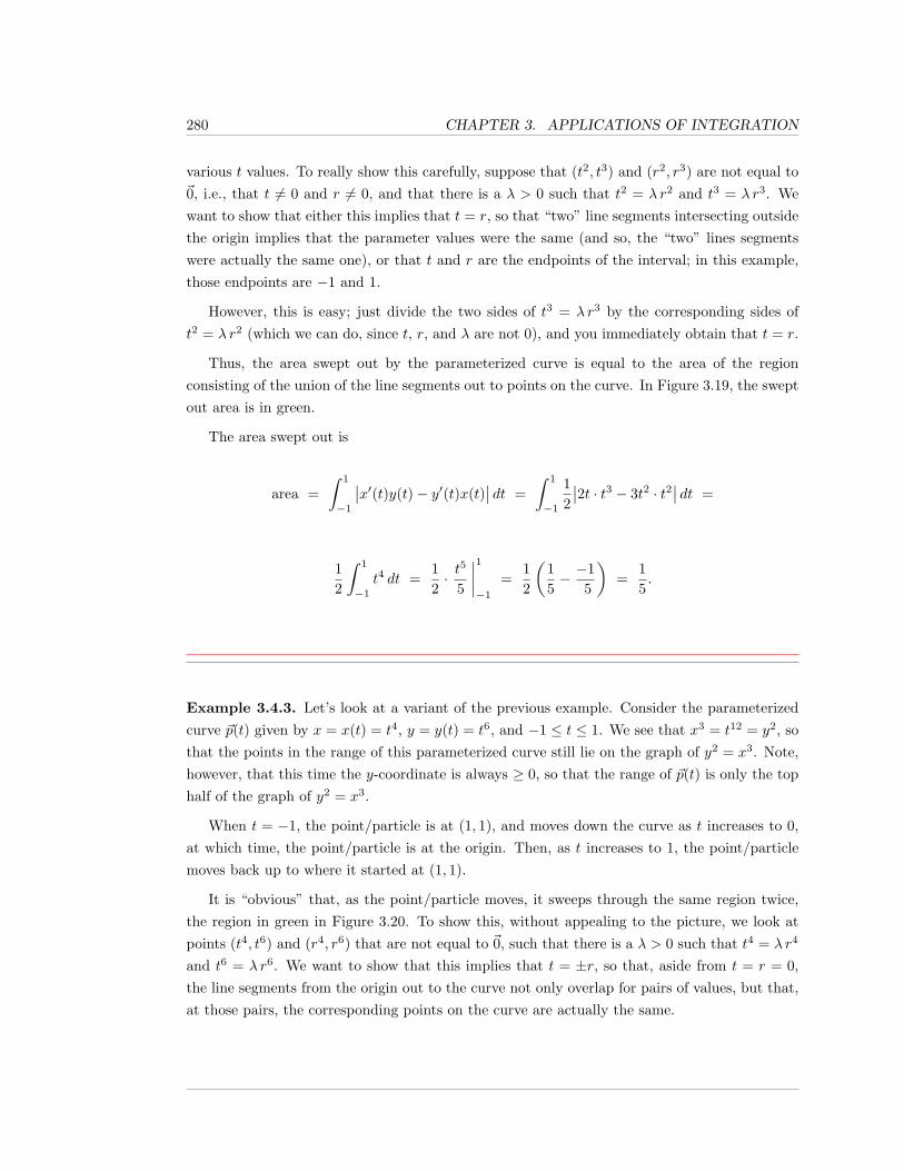
280 CHAPTER 3. APPLICATIONS OF INTEGRATION
various t values. To really show this carefully, suppose that (t2, t3) and (r2, r3) are not equal to~0, i.e., that t 6= 0 and r 6= 0, and that there is a λ > 0 such that t2 = λ r2 and t3 = λ r3. Wewant to show that either this implies that t = r, so that “two” line segments intersecting outsidethe origin implies that the parameter values were the same (and so, the “two” lines segmentswere actually the same one), or that t and r are the endpoints of the interval; in this example,those endpoints are −1 and 1.
However, this is easy; just divide the two sides of t3 = λ r3 by the corresponding sides oft2 = λ r2 (which we can do, since t, r, and λ are not 0), and you immediately obtain that t = r.
Thus, the area swept out by the parameterized curve is equal to the area of the regionconsisting of the union of the line segments out to points on the curve. In Figure 3.19, the sweptout area is in green.
The area swept out is
area =∫ 1
−1
∣∣x′(t)y(t)− y′(t)x(t)∣∣ dt =
∫ 1
−1
12
∣∣2t · t3 − 3t2 · t2∣∣ dt =
12
∫ 1
−1
t4 dt =12· t
5
5
∣∣∣∣1−1
=12
(15− −1
5
)=
15.
Example 3.4.3. Let’s look at a variant of the previous example. Consider the parameterizedcurve ~p(t) given by x = x(t) = t4, y = y(t) = t6, and −1 ≤ t ≤ 1. We see that x3 = t12 = y2, sothat the points in the range of this parameterized curve still lie on the graph of y2 = x3. Note,however, that this time the y-coordinate is always ≥ 0, so that the range of ~p(t) is only the tophalf of the graph of y2 = x3.
When t = −1, the point/particle is at (1, 1), and moves down the curve as t increases to 0,at which time, the point/particle is at the origin. Then, as t increases to 1, the point/particlemoves back up to where it started at (1, 1).
It is “obvious” that, as the point/particle moves, it sweeps through the same region twice,the region in green in Figure 3.20. To show this, without appealing to the picture, we look atpoints (t4, t6) and (r4, r6) that are not equal to ~0, such that there is a λ > 0 such that t4 = λ r4
and t6 = λ r6. We want to show that this implies that t = ±r, so that, aside from t = r = 0,the line segments from the origin out to the curve not only overlap for pairs of values, but that,at those pairs, the corresponding points on the curve are actually the same.
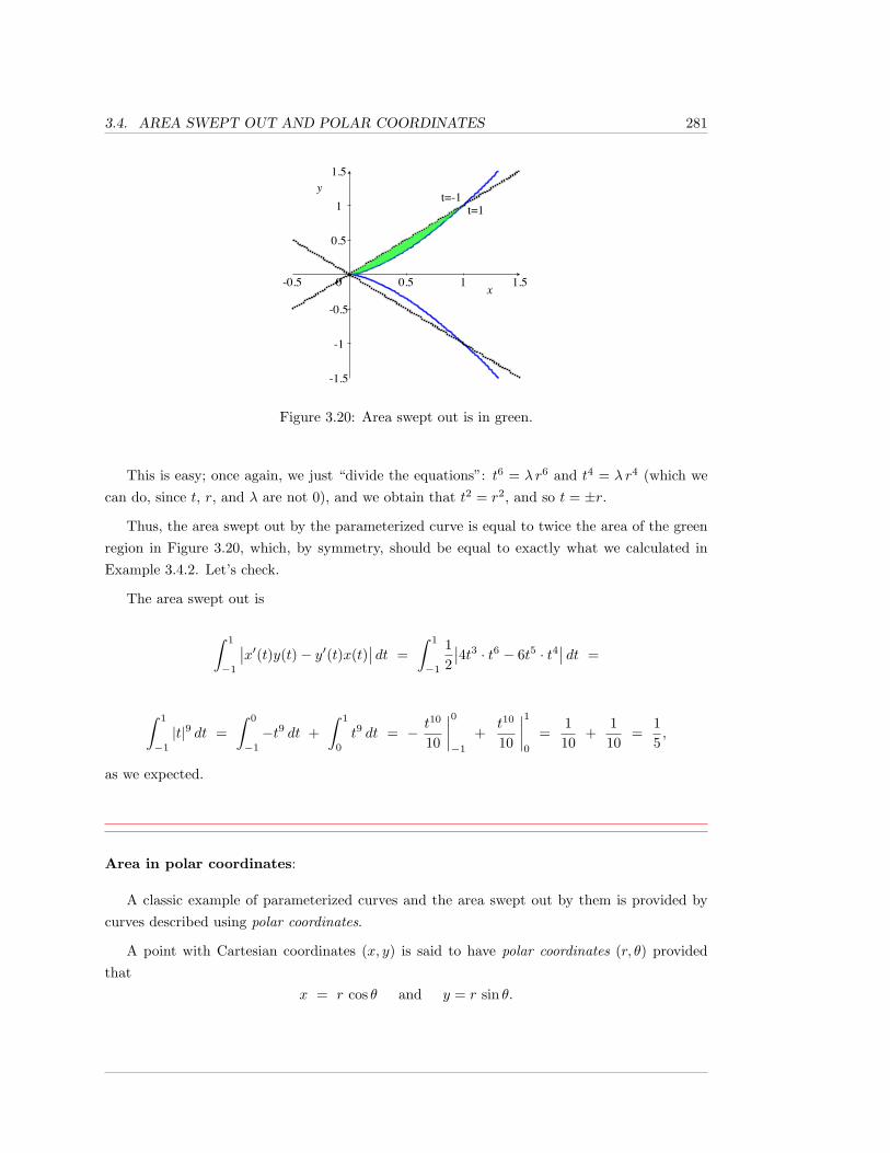
3.4. AREA SWEPT OUT AND POLAR COORDINATES 281
-0.5 0 0.5 1 1.5
-1.5
-1
-0.5
0.5
1
1.5
t=-1t=1
Figure 3.20: Area swept out is in green.
This is easy; once again, we just “divide the equations”: t6 = λ r6 and t4 = λ r4 (which wecan do, since t, r, and λ are not 0), and we obtain that t2 = r2, and so t = ±r.
Thus, the area swept out by the parameterized curve is equal to twice the area of the greenregion in Figure 3.20, which, by symmetry, should be equal to exactly what we calculated inExample 3.4.2. Let’s check.
The area swept out is
∫ 1
−1
∣∣x′(t)y(t)− y′(t)x(t)∣∣ dt =
∫ 1
−1
12
∣∣4t3 · t6 − 6t5 · t4∣∣ dt =
∫ 1
−1
|t|9 dt =∫ 0
−1
−t9 dt +∫ 1
0
t9 dt = − t10
10
∣∣∣∣0−1
+t10
10
∣∣∣∣10
=110
+110
=15,
as we expected.
Area in polar coordinates:
A classic example of parameterized curves and the area swept out by them is provided bycurves described using polar coordinates.
A point with Cartesian coordinates (x, y) is said to have polar coordinates (r, θ) providedthat
x = r cos θ and y = r sin θ.
282 CHAPTER 3. APPLICATIONS OF INTEGRATION
You should realize immediately that this definition, and the periodicity of sine and cosine,imply that every point (x, y) possesses an infinite number of polar coordinates! For instance,the point (x, y) = (1, 1) has polar coordinates (r, θ) = (
√2, π/4), (r, θ) = (−
√2, 3π/4), and,
more generally, polar coordinates
(r, θ) =(
(−1)n√
2,π
4+ nπ
),
where n is any integer. Even worse, the origin, (x, y) = (0, 0) has polar coordinates r = 0 andθ = any real number!
Be aware that some sources require that r ≥ 0 in polar coordinates. While this conventionmakes polar coordinates slightly easier to deal with, it destroys our ability to easily describesome beautiful curves in terms of polar coordinates. We shall not assume that r must benon-negative.
Given r and θ for a point P , it is easy to produce the Cartesian coordinates of P ; you simplyuse that x = r cos θ and y = r sin θ. The question is: given x and y, how do you produce one
corresponding set of polar coordinates, i.e., given x and y, how do you produce a simultaneoussolution to x = r cos θ and y = r sin θ?
Squaring and adding yields
x2 + y2 = r2 cos2 θ + r2 sin2 θ = r2.
Thus, r = ±√x2 + y2.
We see, of course, that r = 0 if and only if the point is the origin. If we are considering apoint other than the origin, and decide to use a positive r, then we must have r =
√x2 + y2,
and then a θ, where 0 ≤ θ < 2π, is uniquely determined by dividing the equations x = r cos θand y = r sin θ by r to obtain:
cos θ =x√
x2 + y2and sin θ =
y√x2 + y2
.
At this point, you can use inverse trig functions to obtain a θ, as long as you’re careful aboutwhat quadrant the point is in. Once you have one pair of polar coordinates (r0, θ0) for apoint (other than the origin), every other pair that represents the same point is of the form((−1)nr0, θ0 + nπ)
)for integer values of n.
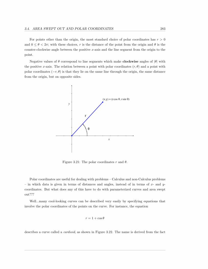
3.4. AREA SWEPT OUT AND POLAR COORDINATES 283
For points other than the origin, the most standard choice of polar coordinates has r > 0and 0 ≤ θ < 2π; with these choices, r is the distance of the point from the origin and θ is thecounter-clockwise angle between the positive x-axis and the line segment from the origin to thepoint.
Negative values of θ correspond to line segments which make clockwise angles of |θ| withthe positive x-axis. The relation between a point with polar coordinates (r, θ) and a point withpolar coordinates (−r, θ) is that they lie on the same line through the origin, the same distancefrom the origin, but on opposite sides.
r
θ
(x,y) = (r cos θ, r sin θ)
Figure 3.21: The polar coordinates r and θ.
Polar coordinates are useful for dealing with problems – Calculus and non-Calculus problems– in which data is given in terms of distances and angles, instead of in terms of x- and y-coordinates. But what does any of this have to do with parameterized curves and area sweptout???
Well...many cool-looking curves can be described very easily by specifying equations thatinvolve the polar coordinates of the points on the curve. For instance, the equation
r = 1 + cos θ
describes a curve called a cardioid, as shown in Figure 3.22. The name is derived from the fact
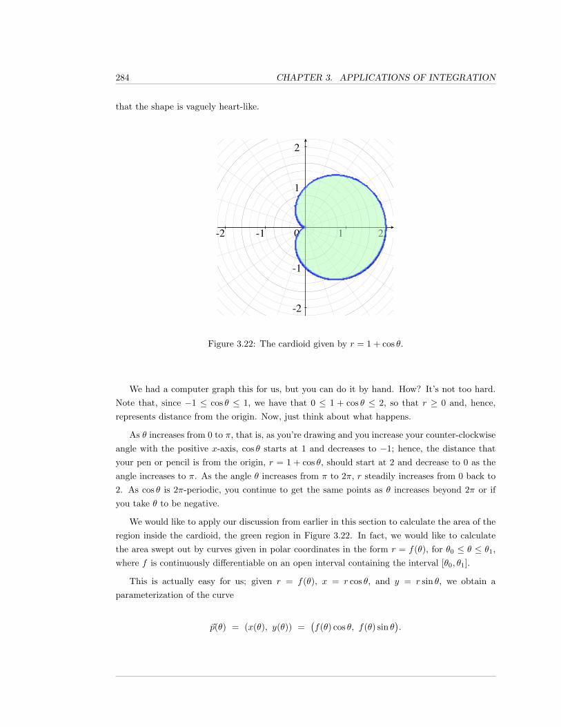
284 CHAPTER 3. APPLICATIONS OF INTEGRATION
that the shape is vaguely heart-like.
-2 -1 0 1 2
-2
-1
1
2
Figure 3.22: The cardioid given by r = 1 + cos θ.
We had a computer graph this for us, but you can do it by hand. How? It’s not too hard.Note that, since −1 ≤ cos θ ≤ 1, we have that 0 ≤ 1 + cos θ ≤ 2, so that r ≥ 0 and, hence,represents distance from the origin. Now, just think about what happens.
As θ increases from 0 to π, that is, as you’re drawing and you increase your counter-clockwiseangle with the positive x-axis, cos θ starts at 1 and decreases to −1; hence, the distance thatyour pen or pencil is from the origin, r = 1 + cos θ, should start at 2 and decrease to 0 as theangle increases to π. As the angle θ increases from π to 2π, r steadily increases from 0 back to2. As cos θ is 2π-periodic, you continue to get the same points as θ increases beyond 2π or ifyou take θ to be negative.
We would like to apply our discussion from earlier in this section to calculate the area of theregion inside the cardioid, the green region in Figure 3.22. In fact, we would like to calculatethe area swept out by curves given in polar coordinates in the form r = f(θ), for θ0 ≤ θ ≤ θ1,where f is continuously differentiable on an open interval containing the interval [θ0, θ1].
This is actually easy for us; given r = f(θ), x = r cos θ, and y = r sin θ, we obtain aparameterization of the curve
~p(θ) = (x(θ), y(θ)) =(f(θ) cos θ, f(θ) sin θ
).
3.4. AREA SWEPT OUT AND POLAR COORDINATES 285
The area swept out by the curve as θ goes from θ0 to θ1, where θ0 ≤ θ1 is thus, by Proposi-tion 3.4.1, equal to
∫ θ1
θ0
12
∣∣∣[f(θ) cos θ]′f(θ) sin θ −
[f(θ) sin θ
]′f(θ) cos θ
∣∣∣ dθ.
We leave it as an exercise for you to verify that this integrand simplifies greatly and yieldsthe expression in the proposition below.
Proposition 3.4.4. Suppose that f is continuously differentiable on an open interval con-taining the interval [θ0, θ1]. Then, the area swept out by the parameterized curve given inpolar coordinates by r = f(θ), where θ0 ≤ θ ≤ θ1, is
∫ θ1
θ0
12r2 dθ =
∫ θ1
θ0
12
[f(θ)]2 dθ.
Example 3.4.5. Let’s apply Proposition 3.4.4 to calculate the area inside the curve given byr = 1 + cos θ. Note that, when we discussed drawing this curve, it was clear that there were nooverlapping line segments from the origin out to the curve for 0 ≤ θ < 2π (at points other thanthe origin). The line segment when θ = 0 and when θ = 2π are/is the same, but that’s allowedin Proposition 3.4.1 and doesn’t affect the area calculation.
Therefore, the area inside the cardioid given by r = 1 + cos θ is
12
∫ 2π
0
(1 + cos θ)2 dθ =12
∫ 2π
0
(1 + 2 cos θ + cos2 θ) dθ.
The hard part of this integral is integrating cos2 θ. You either use Proposition 1.2.5, withn = 2, or use the trig identity cos2 θ = (1 + cos(2θ))/2 and an easy substitution of u = 2θ. Oneway or the other, you need to find that
∫cos2 θ dθ = (θ + cos θ sin θ)/2 + C, so that our area
integral above becomes
12
(θ + 2 sin θ +
12(θ + cos θ sin θ
))∣∣∣∣2π0
=3π2.
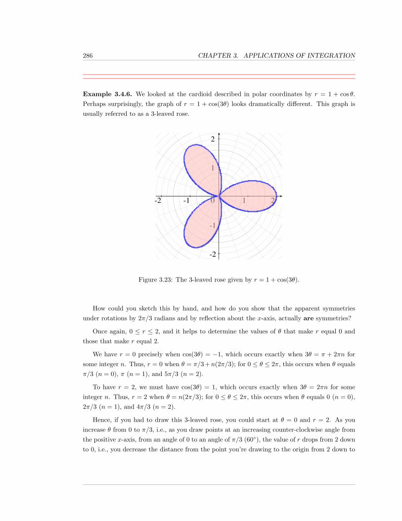
286 CHAPTER 3. APPLICATIONS OF INTEGRATION
Example 3.4.6. We looked at the cardioid described in polar coordinates by r = 1 + cos θ.Perhaps surprisingly, the graph of r = 1 + cos(3θ) looks dramatically different. This graph isusually referred to as a 3-leaved rose.
-2 -1 0 1 2
-2
-1
1
2
Figure 3.23: The 3-leaved rose given by r = 1 + cos(3θ).
How could you sketch this by hand, and how do you show that the apparent symmetriesunder rotations by 2π/3 radians and by reflection about the x-axis, actually are symmetries?
Once again, 0 ≤ r ≤ 2, and it helps to determine the values of θ that make r equal 0 andthose that make r equal 2.
We have r = 0 precisely when cos(3θ) = −1, which occurs exactly when 3θ = π + 2πn forsome integer n. Thus, r = 0 when θ = π/3 +n(2π/3); for 0 ≤ θ ≤ 2π, this occurs when θ equalsπ/3 (n = 0), π (n = 1), and 5π/3 (n = 2).
To have r = 2, we must have cos(3θ) = 1, which occurs exactly when 3θ = 2πn for someinteger n. Thus, r = 2 when θ = n(2π/3); for 0 ≤ θ ≤ 2π, this occurs when θ equals 0 (n = 0),2π/3 (n = 1), and 4π/3 (n = 2).
Hence, if you had to draw this 3-leaved rose, you could start at θ = 0 and r = 2. As youincrease θ from 0 to π/3, i.e., as you draw points at an increasing counter-clockwise angle fromthe positive x-axis, from an angle of 0 to an angle of π/3 (60◦), the value of r drops from 2 downto 0, i.e., you decrease the distance from the point you’re drawing to the origin from 2 down to
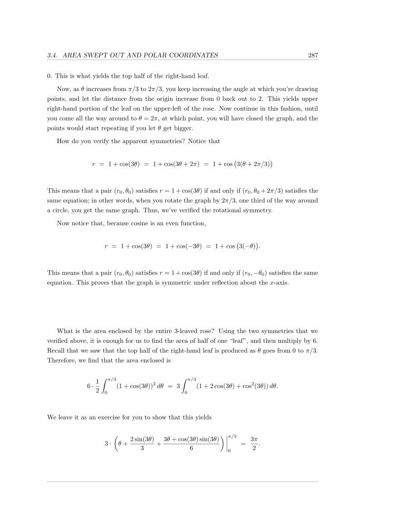
3.4. AREA SWEPT OUT AND POLAR COORDINATES 287
0. This is what yields the top half of the right-hand leaf.
Now, as θ increases from π/3 to 2π/3, you keep increasing the angle at which you’re drawingpoints, and let the distance from the origin increase from 0 back out to 2. This yields upperright-hand portion of the leaf on the upper-left of the rose. Now continue in this fashion, untilyou come all the way around to θ = 2π, at which point, you will have closed the graph, and thepoints would start repeating if you let θ get bigger.
How do you verify the apparent symmetries? Notice that
r = 1 + cos(3θ) = 1 + cos(3θ + 2π) = 1 + cos(3(θ + 2π/3)
)
This means that a pair (r0, θ0) satisfies r = 1 + cos(3θ) if and only if (r0, θ0 + 2π/3) satisfies thesame equation; in other words, when you rotate the graph by 2π/3, one third of the way arounda circle, you get the same graph. Thus, we’ve verified the rotational symmetry.
Now notice that, because cosine is an even function,
r = 1 + cos(3θ) = 1 + cos(−3θ) = 1 + cos(3(−θ)
).
This means that a pair (r0, θ0) satisfies r = 1 + cos(3θ) if and only if (r0,−θ0) satisfies the sameequation. This proves that the graph is symmetric under reflection about the x-axis.
What is the area enclosed by the entire 3-leaved rose? Using the two symmetries that weverified above, it is enough for us to find the area of half of one “leaf”, and then multiply by 6.Recall that we saw that the top half of the right-hand leaf is produced as θ goes from 0 to π/3.Therefore, we find that the area enclosed is
6 · 12
∫ π/3
0
(1 + cos(3θ))2 dθ = 3∫ π/3
0
(1 + 2 cos(3θ) + cos2(3θ)) dθ.
We leave it as an exercise for you to show that this yields
3 ·(θ +
2 sin(3θ)3
+3θ + cos(3θ) sin(3θ)
6
) ∣∣∣∣π/30
=3π2.
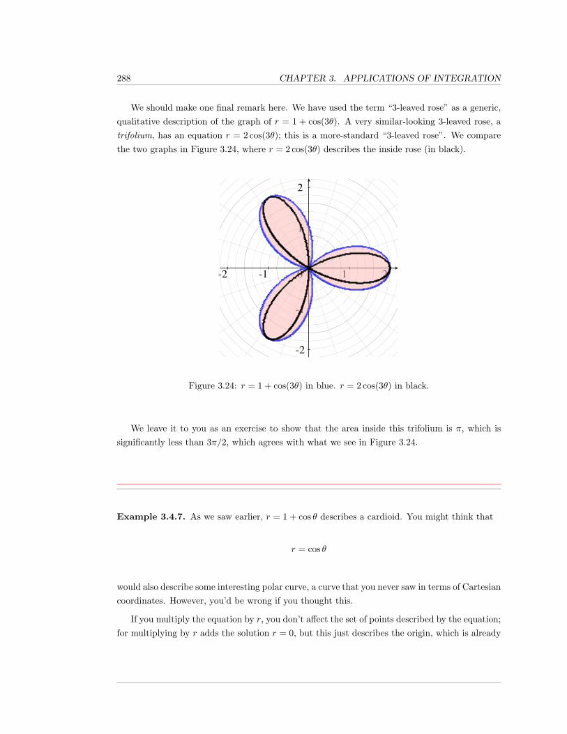
288 CHAPTER 3. APPLICATIONS OF INTEGRATION
We should make one final remark here. We have used the term “3-leaved rose” as a generic,qualitative description of the graph of r = 1 + cos(3θ). A very similar-looking 3-leaved rose, atrifolium, has an equation r = 2 cos(3θ); this is a more-standard “3-leaved rose”. We comparethe two graphs in Figure 3.24, where r = 2 cos(3θ) describes the inside rose (in black).
-2 -1 0 1 2
-2
-1
1
2
Figure 3.24: r = 1 + cos(3θ) in blue. r = 2 cos(3θ) in black.
We leave it to you as an exercise to show that the area inside this trifolium is π, which issignificantly less than 3π/2, which agrees with what we see in Figure 3.24.
Example 3.4.7. As we saw earlier, r = 1 + cos θ describes a cardioid. You might think that
r = cos θ
would also describe some interesting polar curve, a curve that you never saw in terms of Cartesiancoordinates. However, you’d be wrong if you thought this.
If you multiply the equation by r, you don’t affect the set of points described by the equation;for multiplying by r adds the solution r = 0, but this just describes the origin, which is already
3.4. AREA SWEPT OUT AND POLAR COORDINATES 289
a point on the curve, since 0 = cos(π/2). Thus, the curve may be described by
r2 = r cos θ.
But this is easy to change into Cartesian coordinates; the equation becomes
x2 + y2 = x.
Subtracting x from each side, and completing the square yields
x2 − x+ y2 = 0 and so(x− 1
2
)2
+ y2 =14,
which, hopefully, you recognize as an equation for a circle of radius 1/2, centered at (1/2, 0).
You should convince yourself that, in polar coordinates, this circle is swept out as θ goesfrom 0 to π; if you went to 2π, you’d sweep out the circle twice.
Of course, we know that the area inside a circle of radius 1/2 is π(1/2)2 = π/4, but we can“check” this by calculating the integral
∫ π
0
12r2 dθ =
∫ π
0
12
cos2 θ dθ.
As we saw in Proposition 1.2.5,∫
cos2 θ dθ = (θ + cos θ sin θ)/2 + C, and so, we conclude that
area =θ + cos θ sin θ
4
∣∣∣∣π0
=π
4.
3.4.1 Exercises
In Exercises 1 through 5, you are given the component functions x = x(t) and y = y(t)for a parameterized curve. a) Find the area swept out by the parameterized curve
290 CHAPTER 3. APPLICATIONS OF INTEGRATION
over the given interval. b) Think of the parameterized curve as giving the position,
at time t, of a particle in the xy-plane. Eliminate the parameter t, to arrive at an
equation containing only x and y; sketch the graph of this curve, and decide how
the particle moves along the curve during the given times. Shade in the area swept
out.
1. x = t, y = t2; 0 ≤ t ≤ 2.
2. x = sin t, y = cos t;π
2≤ t ≤ π.
3. x = t3, y = t2; −1 ≤ t ≤ 1.
4. x = e2t, y = e3t; −1 ≤ t ≤ 1.
5. x = ln t, y = t; 1 ≤ t ≤ 3
6. Suppose that a > b > 0. Find the area swept out by the curve ~p(t) = (ta, tb), for t in theinterval [0, 1].
In Exercises 7 through 12, you are given a curve r = f(θ), described in polar coor-
dinates. Sketch the curve and find the area it encloses.
7. r = 1 + sin θ.
8. r = 1 + sin(4θ).
9. r = 5 + 4 cos θ.
10. r2 = 9 sin(2θ).
11. r = 2(1 + sin θ).
12. r = 3 cos(5θ).
13. Find the area inside the big loop and outside the small loop of the graph of r =12
+ sin θ;this figure is known as a limacon. See Figure 3.25.
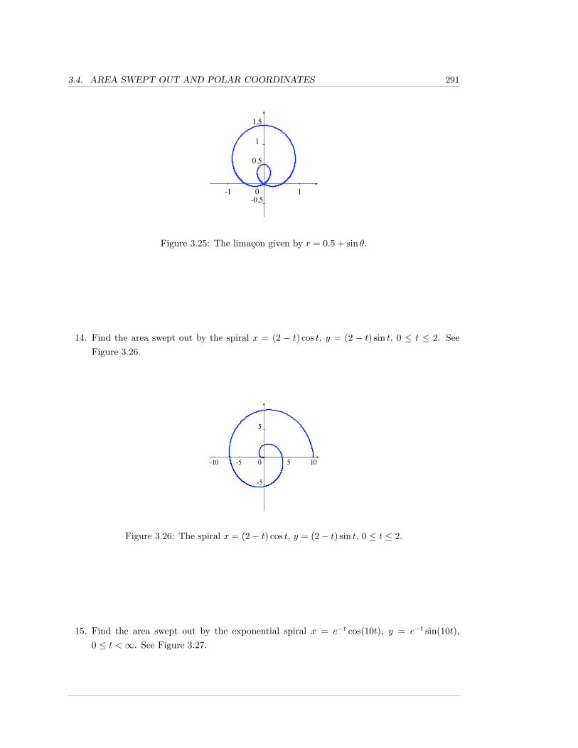
3.4. AREA SWEPT OUT AND POLAR COORDINATES 291
-1 0 1-0.5
0.5
1
1.5
Figure 3.25: The limacon given by r = 0.5 + sin θ.
14. Find the area swept out by the spiral x = (2 − t) cos t, y = (2 − t) sin t, 0 ≤ t ≤ 2. SeeFigure 3.26.
-10 -5 0 5 10
-5
5
Figure 3.26: The spiral x = (2− t) cos t, y = (2− t) sin t, 0 ≤ t ≤ 2.
15. Find the area swept out by the exponential spiral x = e−t cos(10t), y = e−t sin(10t),0 ≤ t <∞. See Figure 3.27.
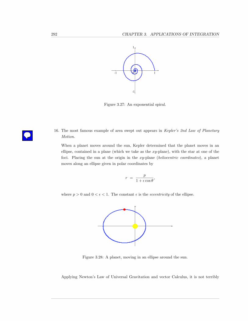
292 CHAPTER 3. APPLICATIONS OF INTEGRATION
-1 0 1
-1
1
Figure 3.27: An exponential spiral.
16. The most famous example of area swept out appears in Kepler’s 2nd Law of PlanetaryMotion.
When a planet moves around the sun, Kepler determined that the planet moves in anellipse, contained in a plane (which we take as the xy-plane), with the star at one of thefoci. Placing the sun at the origin in the xy-plane (heliocentric coordinates), a planetmoves along an ellipse given in polar coordinates by
r =p
1 + ε cos θ,
where p > 0 and 0 < ε < 1. The constant ε is the eccentricity of the ellipse.
Figure 3.28: A planet, moving in an ellipse around the sun.
Applying Newton’s Law of Universal Gravitation and vector Calculus, it is not terribly
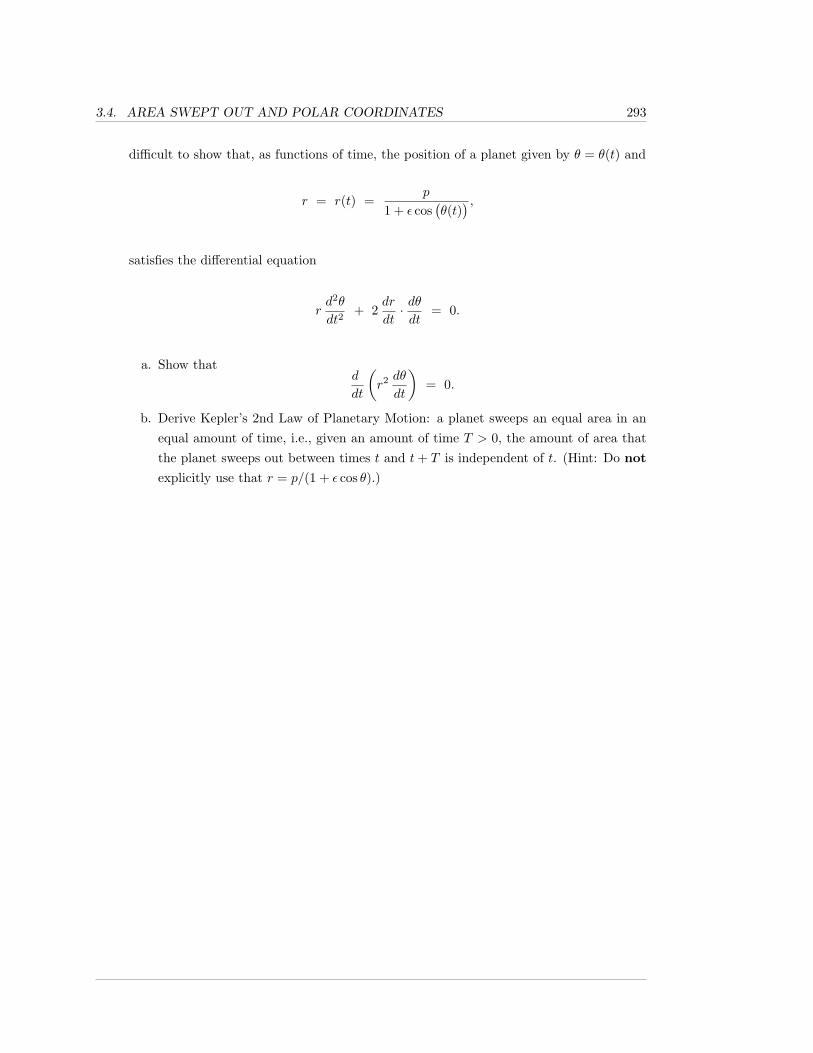
3.4. AREA SWEPT OUT AND POLAR COORDINATES 293
difficult to show that, as functions of time, the position of a planet given by θ = θ(t) and
r = r(t) =p
1 + ε cos(θ(t)
) ,satisfies the differential equation
rd2θ
dt2+ 2
dr
dt· dθdt
= 0.
a. Show thatd
dt
(r2 dθ
dt
)= 0.
b. Derive Kepler’s 2nd Law of Planetary Motion: a planet sweeps an equal area in anequal amount of time, i.e., given an amount of time T > 0, the amount of area thatthe planet sweeps out between times t and t+ T is independent of t. (Hint: Do not
explicitly use that r = p/(1 + ε cos θ).)
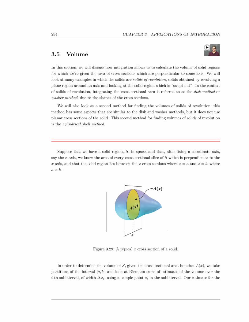
294 CHAPTER 3. APPLICATIONS OF INTEGRATION
3.5 Volume
In this section, we will discuss how integration allows us to calculate the volume of solid regionsfor which we’re given the area of cross sections which are perpendicular to some axis. We willlook at many examples in which the solids are solids of revolution, solids obtained by revolving aplane region around an axis and looking at the solid region which is “swept out”. In the contextof solids of revolution, integrating the cross-sectional area is referred to as the disk method orwasher method, due to the shapes of the cross sections.
We will also look at a second method for finding the volumes of solids of revolution; thismethod has some aspects that are similar to the disk and washer methods, but it does not useplanar cross sections of the solid. This second method for finding volumes of solids of revolutionis the cylindrical shell method.
Suppose that we have a solid region, S, in space, and that, after fixing a coordinate axis,say the x-axis, we know the area of every cross-sectional slice of S which is perpendicular to thex-axis, and that the solid region lies between the x cross sections where x = a and x = b, wherea < b.
A(x)A(x)
x
xixi-1si
¢xiFigure 3.29: A typical x cross section of a solid.
In order to determine the volume of S, given the cross-sectional area function A(x), we takepartitions of the interval [a, b], and look at Riemann sums of estimates of the volume over thei-th subinterval, of width ∆xi, using a sample point si in the subinterval. Our estimate for the
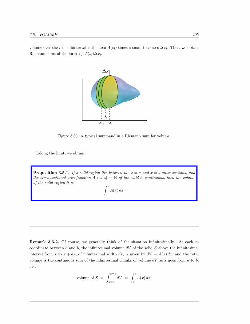
3.5. VOLUME 295
volume over the i-th subinterval is the area A(si) times a small thickness ∆xi. Thus, we obtainRiemann sums of the form
∑iA(si)∆xi.
A(x)A(x)
x
xixi-1si
¢xi
Figure 3.30: A typical summand in a Riemann sum for volume.
Taking the limit, we obtain:
Proposition 3.5.1. If a solid region lies between the x = a and x = b cross sections, andthe cross-sectional area function A : [a, b] → R of the solid is continuous, then the volumeof the solid region S is ∫ b
a
A(x) dx.
Remark 3.5.2. Of course, we generally think of the situation infinitesimally. At each x-coordinate between a and b, the infinitesimal volume dV of the solid S above the infinitesimalinterval from x to x + dx, of infinitesimal width dx, is given by dV = A(x) dx, and the totalvolume is the continuous sum of the infinitesimal chunks of volume dV as x goes from a to b,i.e.,
volume of S =∫ x=b
x=a
dV =∫ b
a
A(x) dx.
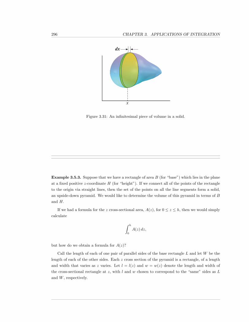
296 CHAPTER 3. APPLICATIONS OF INTEGRATION
A(x)A(x)
x
xixi-1si
¢xi
Figure 3.31: An infinitesimal piece of volume in a solid.
Example 3.5.3. Suppose that we have a rectangle of area B (for “base”) which lies in the planeat a fixed positive z-coordinate H (for “height”). If we connect all of the points of the rectangleto the origin via straight lines, then the set of the points on all the line segments form a solid,an upside-down pyramid. We would like to determine the volume of this pyramid in terms of Band H.
If we had a formula for the z cross-sectional area, A(z), for 0 ≤ z ≤ h, then we would simplycalculate
∫ h
0
A(z) dz,
but how do we obtain a formula for A(z)?
Call the length of each of one pair of parallel sides of the base rectangle L and let W be thelength of each of the other sides. Each z cross section of the pyramid is a rectangle, of a lengthand width that varies as z varies. Let l = l(z) and w = w(z) denote the length and width ofthe cross-sectional rectangle at z, with l and w chosen to correspond to the “same” sides as Land W , respectively.
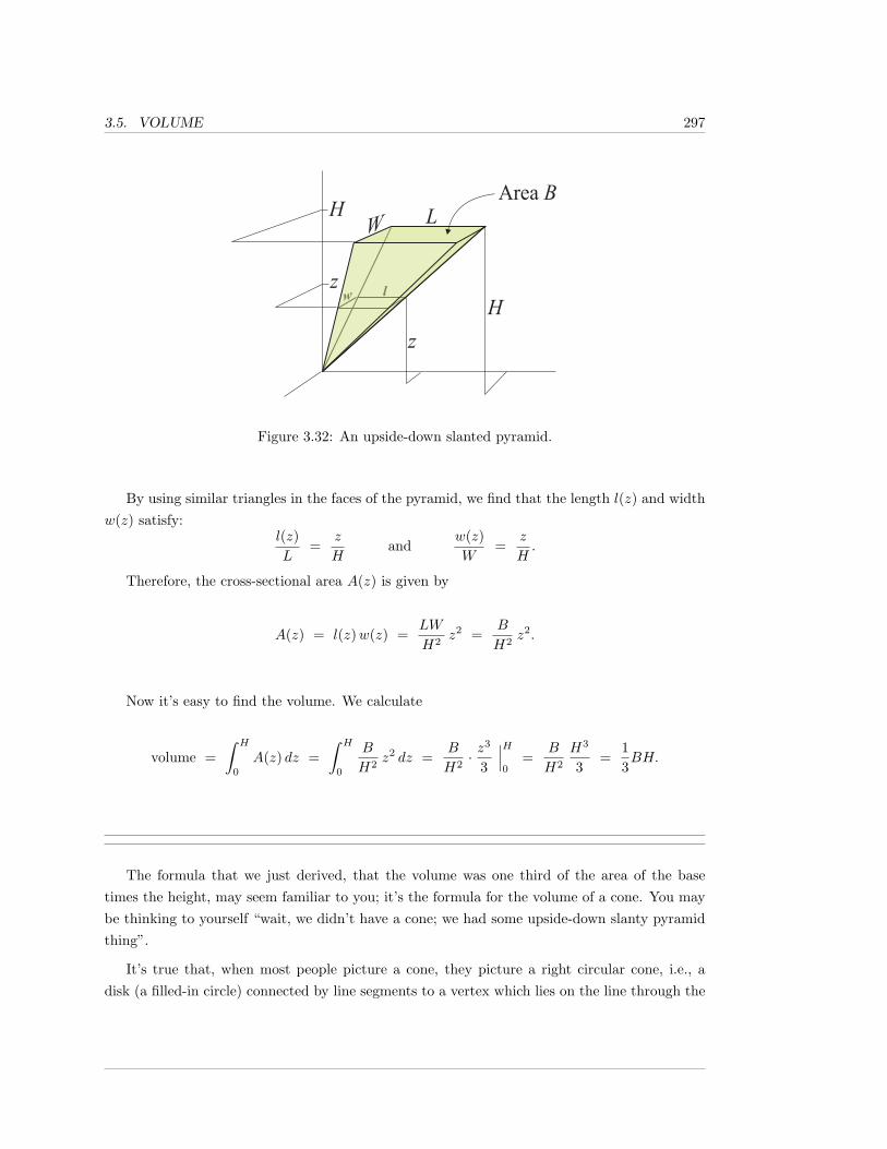
3.5. VOLUME 297
W
lwL
H
H
z
Area B
z
H
z
H
z
Figure 3.32: An upside-down slanted pyramid.
By using similar triangles in the faces of the pyramid, we find that the length l(z) and widthw(z) satisfy:
l(z)L
=z
Hand
w(z)W
=z
H.
Therefore, the cross-sectional area A(z) is given by
A(z) = l(z)w(z) =LW
H2z2 =
B
H2z2.
Now it’s easy to find the volume. We calculate
volume =∫ H
0
A(z) dz =∫ H
0
B
H2z2 dz =
B
H2· z
3
3
∣∣∣H0
=B
H2
H3
3=
13BH.
The formula that we just derived, that the volume was one third of the area of the basetimes the height, may seem familiar to you; it’s the formula for the volume of a cone. You maybe thinking to yourself “wait, we didn’t have a cone; we had some upside-down slanty pyramidthing”.
It’s true that, when most people picture a cone, they picture a right circular cone, i.e., adisk (a filled-in circle) connected by line segments to a vertex which lies on the line through the
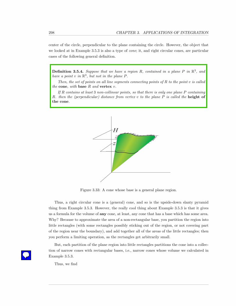
298 CHAPTER 3. APPLICATIONS OF INTEGRATION
center of the circle, perpendicular to the plane containing the circle. However, the object thatwe looked at in Example 3.5.3 is also a type of cone; it, and right circular cones, are particularcases of the following general definition.
Definition 3.5.4. Suppose that we have a region R, contained in a plane P in R3, andhave a point v in R3, but not in the plane P .
Then, the set of points on all line segments connecting points of R to the point v is calledthe cone, with base R and vertex v.
If R contains at least 3 non-collinear points, so that there is only one plane P containingR. then the (perpendicular) distance from vertex v to the plane P is called the height ofthe cone.
W
lwL
H
H
z
Area B
z
H
z
Figure 3.33: A cone whose base is a general plane region.
Thus, a right circular cone is a (general) cone, and so is the upside-down slanty pyramidthing from Example 3.5.3. However, the really cool thing about Example 3.5.3 is that it givesus a formula for the volume of any cone, at least, any cone that has a base which has some area.Why? Because to approximate the area of a non-rectangular base, you partition the region intolittle rectangles (with some rectangles possibly sticking out of the region, or not covering partof the region near the boundary), and add together all of the areas of the little rectangles; thenyou perform a limiting operation, as the rectangles get arbitrarily small.
But, each partition of the plane region into little rectangles partitions the cone into a collec-tion of narrow cones with rectangular bases, i.e., narrow cones whose volume we calculated inExample 3.5.3.
Thus, we find
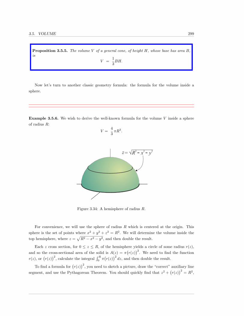
3.5. VOLUME 299
Proposition 3.5.5. The volume V of a general cone, of height H, whose base has area B,is
V =13BH.
Now let’s turn to another classic geometry formula: the formula for the volume inside asphere.
Example 3.5.6. We wish to derive the well-known formula for the volume V inside a sphereof radius R:
V =43πR3.
2 2 z = �R - y2 x - {r(z)R z
Figure 3.34: A hemisphere of radius R.
For convenience, we will use the sphere of radius R which is centered at the origin. Thissphere is the set of points where x2 + y2 + z2 = R2. We will determine the volume inside thetop hemisphere, where z =
√R2 − x2 − y2, and then double the result.
Each z cross section, for 0 ≤ z ≤ R, of the hemisphere yields a circle of some radius r(z),and so the cross-sectional area of the solid is A(z) = π
(r(z)
)2. We need to find the functionr(z), or
(r(z)
)2, calculate the integral∫ R
0π(r(z)
)2dz, and then double the result.
To find a formula for(r(z)
)2, you need to sketch a picture, draw the “correct” auxiliary linesegment, and use the Pythagorean Theorem. You should quickly find that z2 +
(r(z)
)2 = R2,
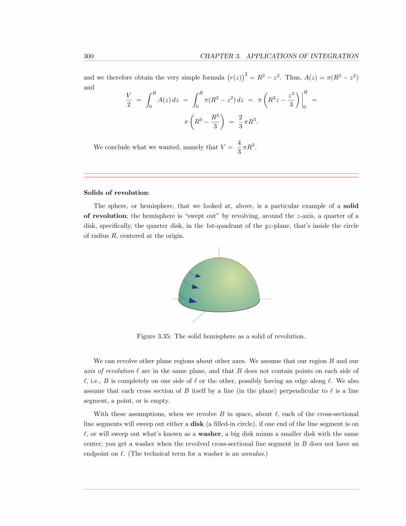
300 CHAPTER 3. APPLICATIONS OF INTEGRATION
and we therefore obtain the very simple formula(r(z)
)2 = R2 − z2. Thus, A(z) = π(R2 − z2)and
V
2=∫ R
0
A(z) dz =∫ R
0
π(R2 − z2) dz = π
(R2z − z3
3
) ∣∣∣∣R0
=
π
(R3 − R3
3
)=
23πR3.
We conclude what we wanted, namely that V =43πR3.
Solids of revolution:
The sphere, or hemisphere, that we looked at, above, is a particular example of a solid
of revolution; the hemisphere is “swept out” by revolving, around the z-axis, a quarter of adisk, specifically, the quarter disk, in the 1st-quadrant of the yz-plane, that’s inside the circleof radius R, centered at the origin.
Figure 3.35: The solid hemisphere as a solid of revolution.
We can revolve other plane regions about other axes. We assume that our region B and ouraxis of revolution ` are in the same plane, and that B does not contain points on each side of`, i.e., B is completely on one side of ` or the other, possibly having an edge along `. We alsoassume that each cross section of B itself by a line (in the plane) perpendicular to ` is a linesegment, a point, or is empty.
With these assumptions, when we revolve B in space, about `, each of the cross-sectionalline segments will sweep out either a disk (a filled-in circle), if one end of the line segment is on`, or will sweep out what’s known as a washer, a big disk minus a smaller disk with the samecenter; you get a washer when the revolved cross-sectional line segment in B does not have anendpoint on `. (The technical term for a washer is an annulus.)
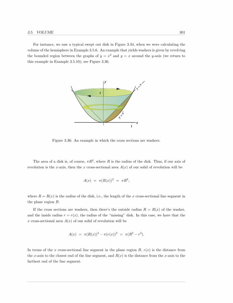
3.5. VOLUME 301
For instance, we saw a typical swept out disk in Figure 3.34, when we were calculating thevolume of the hemisphere in Example 3.5.6. An example that yields washers is given by revolvingthe bounded region between the graphs of y = x2 and y = x around the y-axis (we return tothis example in Example 3.5.10); see Figure 3.36.
1
1
x
y
2y x=y x=
Figure 3.36: An example in which the cross sections are washers.
The area of a disk is, of course, πR2, where R is the radius of the disk. Thus, if our axis ofrevolution is the x-axis, then the x cross-sectional area A(x) of our solid of revolution will be
A(x) = π(R(x))2 = πR2,
where R = R(x) is the radius of the disk, i.e., the length of the x cross-sectional line segment inthe plane region B.
If the cross sections are washers, then there’s the outside radius R = R(x) of the washer,and the inside radius r = r(x), the radius of the “missing” disk. In this case, we have that thex cross-sectional area A(x) of our solid of revolution will be
A(x) = π(R(x))2 − π(r(x))2 = π(R2 − r2).
In terms of the x cross-sectional line segment in the plane region B, r(x) is the distance fromthe x-axis to the closest end of the line segment, and R(x) is the distance from the x-axis to thefarthest end of the line segment.
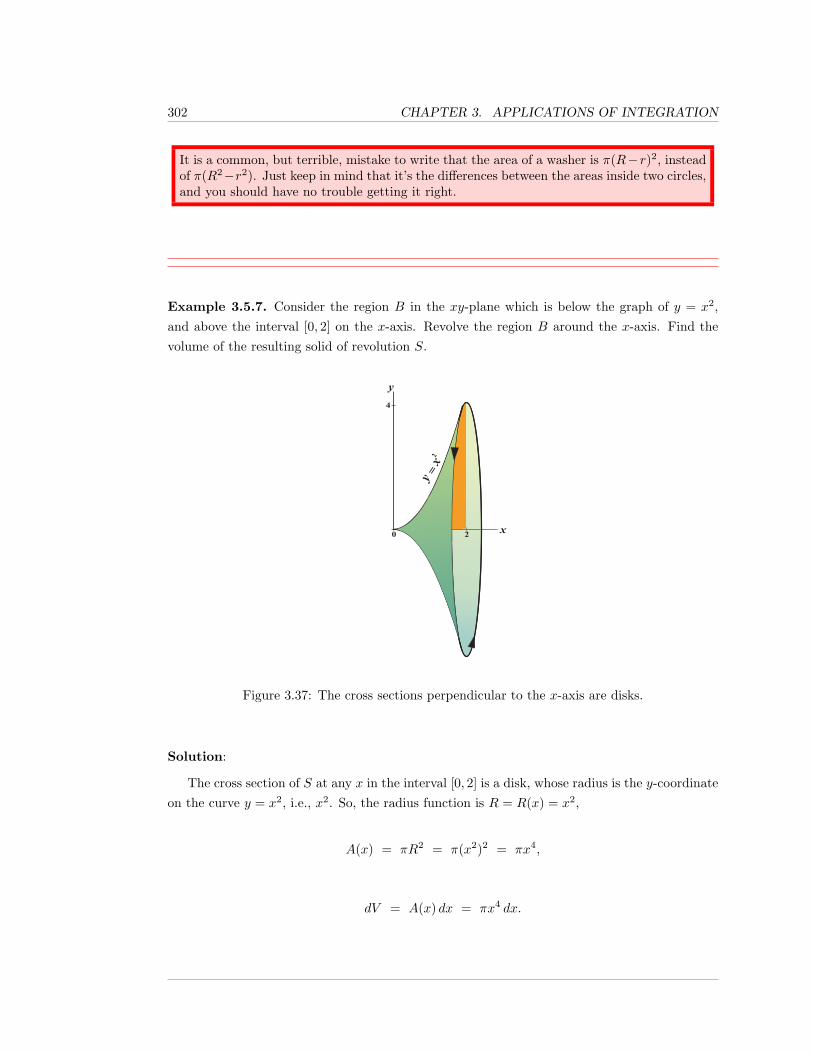
302 CHAPTER 3. APPLICATIONS OF INTEGRATION
It is a common, but terrible, mistake to write that the area of a washer is π(R−r)2, insteadof π(R2−r2). Just keep in mind that it’s the differences between the areas inside two circles,and you should have no trouble getting it right.
Example 3.5.7. Consider the region B in the xy-plane which is below the graph of y = x2,and above the interval [0, 2] on the x-axis. Revolve the region B around the x-axis. Find thevolume of the resulting solid of revolution S.
0
4
x
y2y x=
2
Figure 3.37: The cross sections perpendicular to the x-axis are disks.
Solution:
The cross section of S at any x in the interval [0, 2] is a disk, whose radius is the y-coordinateon the curve y = x2, i.e., x2. So, the radius function is R = R(x) = x2,
A(x) = πR2 = π(x2)2 = πx4,
dV = A(x) dx = πx4 dx.
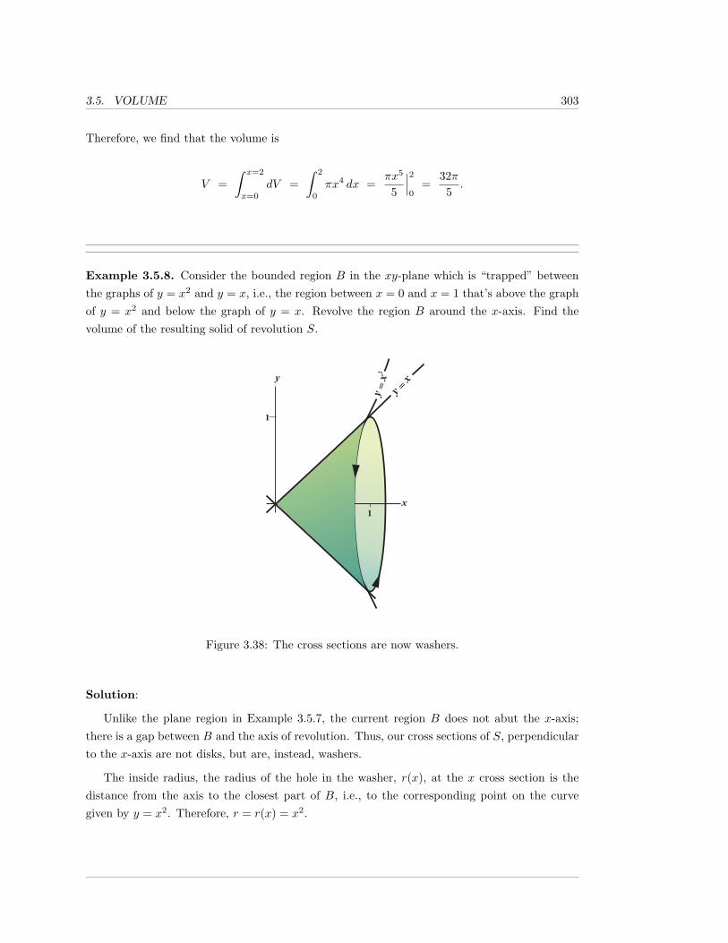
3.5. VOLUME 303
Therefore, we find that the volume is
V =∫ x=2
x=0
dV =∫ 2
0
πx4 dx =πx5
5
∣∣∣20
=32π5.
Example 3.5.8. Consider the bounded region B in the xy-plane which is “trapped” betweenthe graphs of y = x2 and y = x, i.e., the region between x = 0 and x = 1 that’s above the graphof y = x2 and below the graph of y = x. Revolve the region B around the x-axis. Find thevolume of the resulting solid of revolution S.
1
1
x
y 2y x= y x=
Figure 3.38: The cross sections are now washers.
Solution:
Unlike the plane region in Example 3.5.7, the current region B does not abut the x-axis;there is a gap between B and the axis of revolution. Thus, our cross sections of S, perpendicularto the x-axis are not disks, but are, instead, washers.
The inside radius, the radius of the hole in the washer, r(x), at the x cross section is thedistance from the axis to the closest part of B, i.e., to the corresponding point on the curvegiven by y = x2. Therefore, r = r(x) = x2.
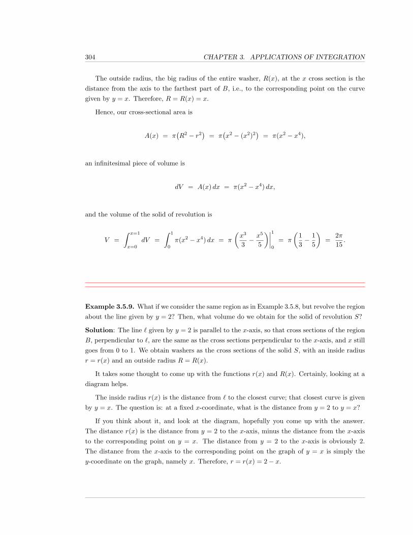
304 CHAPTER 3. APPLICATIONS OF INTEGRATION
The outside radius, the big radius of the entire washer, R(x), at the x cross section is thedistance from the axis to the farthest part of B, i.e., to the corresponding point on the curvegiven by y = x. Therefore, R = R(x) = x.
Hence, our cross-sectional area is
A(x) = π(R2 − r2
)= π
(x2 − (x2)2
)= π(x2 − x4),
an infinitesimal piece of volume is
dV = A(x) dx = π(x2 − x4) dx,
and the volume of the solid of revolution is
V =∫ x=1
x=0
dV =∫ 1
0
π(x2 − x4) dx = π
(x3
3− x5
5
)∣∣∣∣10
= π
(13− 1
5
)=
2π15.
Example 3.5.9. What if we consider the same region as in Example 3.5.8, but revolve the regionabout the line given by y = 2? Then, what volume do we obtain for the solid of revolution S?
Solution: The line ` given by y = 2 is parallel to the x-axis, so that cross sections of the regionB, perpendicular to `, are the same as the cross sections perpendicular to the x-axis, and x stillgoes from 0 to 1. We obtain washers as the cross sections of the solid S, with an inside radiusr = r(x) and an outside radius R = R(x).
It takes some thought to come up with the functions r(x) and R(x). Certainly, looking at adiagram helps.
The inside radius r(x) is the distance from ` to the closest curve; that closest curve is givenby y = x. The question is: at a fixed x-coordinate, what is the distance from y = 2 to y = x?
If you think about it, and look at the diagram, hopefully you come up with the answer.The distance r(x) is the distance from y = 2 to the x-axis, minus the distance from the x-axisto the corresponding point on y = x. The distance from y = 2 to the x-axis is obviously 2.The distance from the x-axis to the corresponding point on the graph of y = x is simply they-coordinate on the graph, namely x. Therefore, r = r(x) = 2− x.
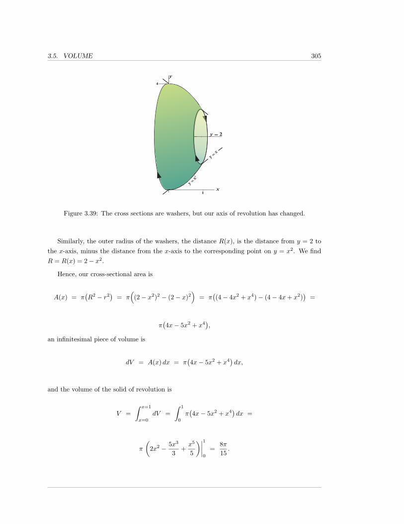
3.5. VOLUME 305
3
1
1
x
y4
2y x=y x=y 2=
Figure 3.39: The cross sections are washers, but our axis of revolution has changed.
Similarly, the outer radius of the washers, the distance R(x), is the distance from y = 2 tothe x-axis, minus the distance from the x-axis to the corresponding point on y = x2. We findR = R(x) = 2− x2.
Hence, our cross-sectional area is
A(x) = π(R2 − r2
)= π
((2− x2)2 − (2− x)2
)= π
((4− 4x2 + x4)− (4− 4x+ x2)
)=
π(4x− 5x2 + x4
),
an infinitesimal piece of volume is
dV = A(x) dx = π(4x− 5x2 + x4
)dx,
and the volume of the solid of revolution is
V =∫ x=1
x=0
dV =∫ 1
0
π(4x− 5x2 + x4
)dx =
π
(2x2 − 5x3
3+x5
5
)∣∣∣∣10
=8π15.
306 CHAPTER 3. APPLICATIONS OF INTEGRATION
Example 3.5.10. What if we consider the same region as in Example 3.5.8, but revolve theregion about the y-axis? Then, what volume do we obtain for the solid of revolution S?
1
1
x
y
2y x=
y x=
Figure 3.40: Washers around the y-axis.
Solution: Now, cross sections perpendicular to our axis of revolution are y cross sections, whichare still washers. However, as we are using y cross sections, we need to write everything in termsof y.
The region B lies between the lines y = 0 and y = 1 (it is a special property of the region Bthat makes the y “limits” the same as the x limits; these would not be the same, in general).
The inside radius r(y) of the cross-sectional washer is the x-coordinate on the closest curveto the axis of revolution, i.e., the x-coordinate on the graph of y = x. Thus, r = r(y) = y. Theoutside radius R(y) is the x-coordinate on the farthest curve, i.e., on the graph of y = x2. Interms of y, this x-coordinate is
√y. Therefore, R = R(y) =
√y.
Hence, our cross-sectional area is
A(y) = π(R2 − r2
)= π
((√y)2 − y2
)= π(y − y2),
an infinitesimal piece of volume is
dV = A(y) dy = π(y − y2) dy,
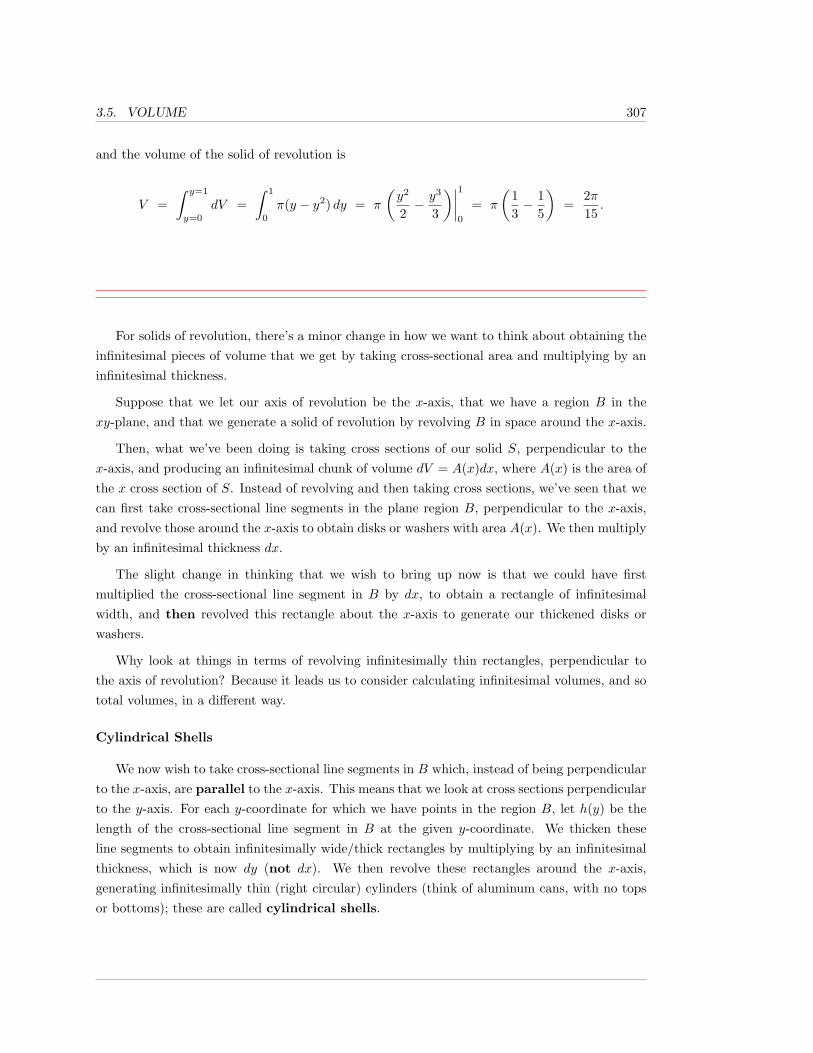
3.5. VOLUME 307
and the volume of the solid of revolution is
V =∫ y=1
y=0
dV =∫ 1
0
π(y − y2) dy = π
(y2
2− y3
3
)∣∣∣∣10
= π
(13− 1
5
)=
2π15.
For solids of revolution, there’s a minor change in how we want to think about obtaining theinfinitesimal pieces of volume that we get by taking cross-sectional area and multiplying by aninfinitesimal thickness.
Suppose that we let our axis of revolution be the x-axis, that we have a region B in thexy-plane, and that we generate a solid of revolution by revolving B in space around the x-axis.
Then, what we’ve been doing is taking cross sections of our solid S, perpendicular to thex-axis, and producing an infinitesimal chunk of volume dV = A(x)dx, where A(x) is the area ofthe x cross section of S. Instead of revolving and then taking cross sections, we’ve seen that wecan first take cross-sectional line segments in the plane region B, perpendicular to the x-axis,and revolve those around the x-axis to obtain disks or washers with area A(x). We then multiplyby an infinitesimal thickness dx.
The slight change in thinking that we wish to bring up now is that we could have firstmultiplied the cross-sectional line segment in B by dx, to obtain a rectangle of infinitesimalwidth, and then revolved this rectangle about the x-axis to generate our thickened disks orwashers.
Why look at things in terms of revolving infinitesimally thin rectangles, perpendicular tothe axis of revolution? Because it leads us to consider calculating infinitesimal volumes, and sototal volumes, in a different way.
Cylindrical Shells
We now wish to take cross-sectional line segments in B which, instead of being perpendicularto the x-axis, are parallel to the x-axis. This means that we look at cross sections perpendicularto the y-axis. For each y-coordinate for which we have points in the region B, let h(y) be thelength of the cross-sectional line segment in B at the given y-coordinate. We thicken theseline segments to obtain infinitesimally wide/thick rectangles by multiplying by an infinitesimalthickness, which is now dy (not dx). We then revolve these rectangles around the x-axis,generating infinitesimally thin (right circular) cylinders (think of aluminum cans, with no topsor bottoms); these are called cylindrical shells.
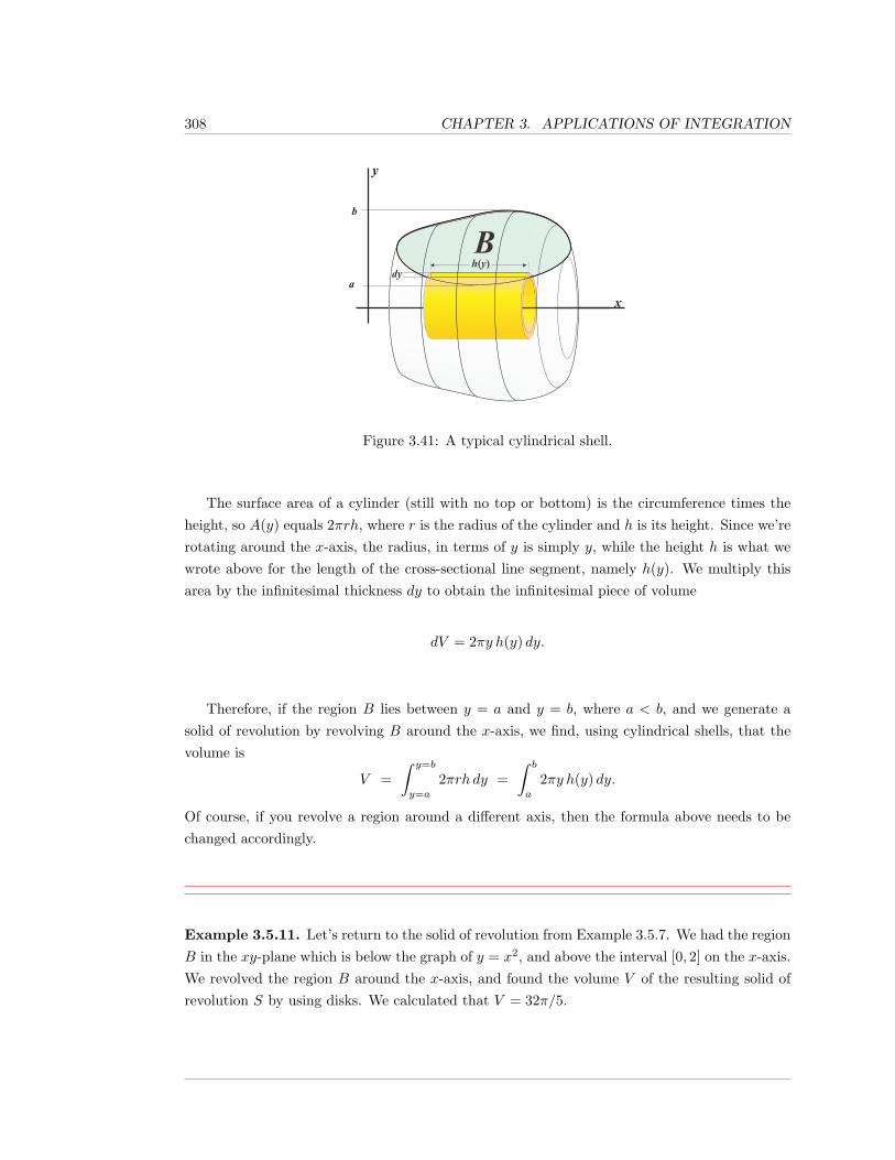
308 CHAPTER 3. APPLICATIONS OF INTEGRATION
h(y)dyaBb
y
x
Figure 3.41: A typical cylindrical shell.
The surface area of a cylinder (still with no top or bottom) is the circumference times theheight, so A(y) equals 2πrh, where r is the radius of the cylinder and h is its height. Since we’rerotating around the x-axis, the radius, in terms of y is simply y, while the height h is what wewrote above for the length of the cross-sectional line segment, namely h(y). We multiply thisarea by the infinitesimal thickness dy to obtain the infinitesimal piece of volume
dV = 2πy h(y) dy.
Therefore, if the region B lies between y = a and y = b, where a < b, and we generate asolid of revolution by revolving B around the x-axis, we find, using cylindrical shells, that thevolume is
V =∫ y=b
y=a
2πrh dy =∫ b
a
2πy h(y) dy.
Of course, if you revolve a region around a different axis, then the formula above needs to bechanged accordingly.
Example 3.5.11. Let’s return to the solid of revolution from Example 3.5.7. We had the regionB in the xy-plane which is below the graph of y = x2, and above the interval [0, 2] on the x-axis.We revolved the region B around the x-axis, and found the volume V of the resulting solid ofrevolution S by using disks. We calculated that V = 32π/5.
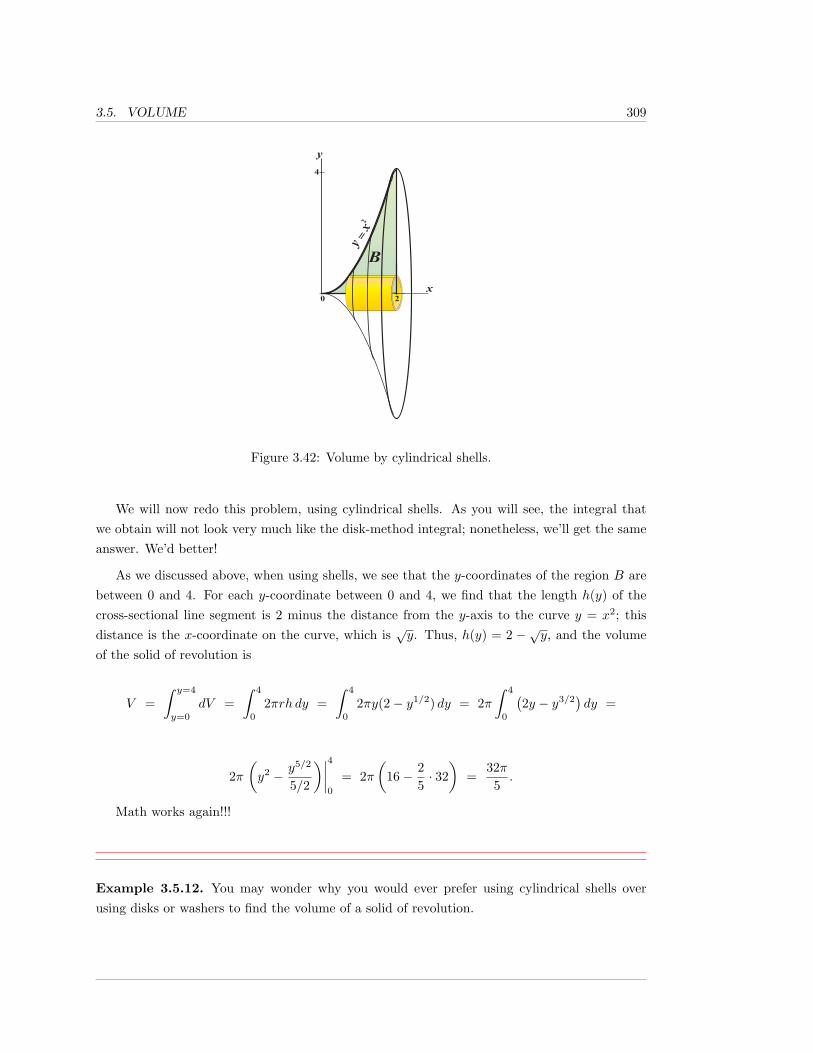
3.5. VOLUME 309
0
4
x
y
2y x=2
B
Figure 3.42: Volume by cylindrical shells.
We will now redo this problem, using cylindrical shells. As you will see, the integral thatwe obtain will not look very much like the disk-method integral; nonetheless, we’ll get the sameanswer. We’d better!
As we discussed above, when using shells, we see that the y-coordinates of the region B arebetween 0 and 4. For each y-coordinate between 0 and 4, we find that the length h(y) of thecross-sectional line segment is 2 minus the distance from the y-axis to the curve y = x2; thisdistance is the x-coordinate on the curve, which is
√y. Thus, h(y) = 2 −√y, and the volume
of the solid of revolution is
V =∫ y=4
y=0
dV =∫ 4
0
2πrh dy =∫ 4
0
2πy(2− y1/2) dy = 2π∫ 4
0
(2y − y3/2
)dy =
2π(y2 − y5/2
5/2
)∣∣∣∣40
= 2π(
16− 25· 32)
=32π5.
Math works again!!!
Example 3.5.12. You may wonder why you would ever prefer using cylindrical shells overusing disks or washers to find the volume of a solid of revolution.
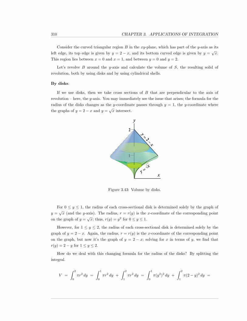
310 CHAPTER 3. APPLICATIONS OF INTEGRATION
Consider the curved triangular region B in the xy-plane, which has part of the y-axis as itsleft edge, its top edge is given by y = 2 − x, and its bottom curved edge is given by y =
√x.
This region lies between x = 0 and x = 1, and between y = 0 and y = 2.
Let’s revolve B around the y-axis and calculate the volume of S, the resulting solid ofrevolution, both by using disks and by using cylindrical shells.
By disks:
If we use disks, then we take cross sections of B that are perpendicular to the axis ofrevolution – here, the y-axis. You may immediately see the issue that arises; the formula for theradius of the disks changes as the y-coordinate passes through y = 1, the y-coordinate wherethe graphs of y = 2− x and y =
√x intersect.
_y 2 x=
xy x=�
2 y
1
Figure 3.43: Volume by disks.
For 0 ≤ y ≤ 1, the radius of each cross-sectional disk is determined solely by the graph ofy =√x (and the y-axis). The radius, r = r(y) is the x-coordinate of the corresponding point
on the graph of y =√x; thus, r(y) = y2 for 0 ≤ y ≤ 1.
However, for 1 ≤ y ≤ 2, the radius of each cross-sectional disk is determined solely by thegraph of y = 2 − x. Again, the radius, r = r(y) is the x-coordinate of the corresponding pointon the graph, but now it’s the graph of y = 2 − x; solving for x in terms of y, we find thatr(y) = 2− y for 1 ≤ y ≤ 2.
How do we deal with this changing formula for the radius of the disks? By splitting theintegral.
V =∫ 2
0
πr2 dy =∫ 1
0
πr2 dy +∫ 2
1
πr2 dy =∫ 1
0
π(y2)2 dy +∫ 2
1
π(2− y)2 dy =
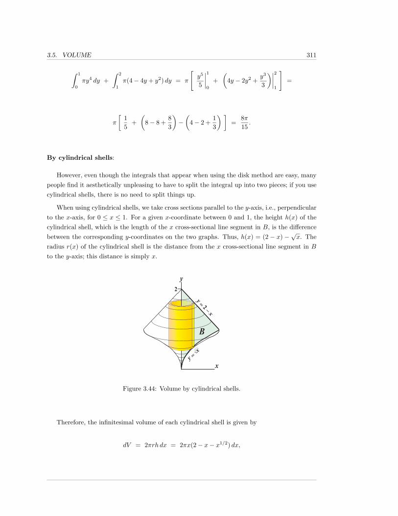
3.5. VOLUME 311
∫ 1
0
πy4 dy +∫ 2
1
π(4− 4y + y2) dy = π
[y5
5
∣∣∣∣10
+(
4y − 2y2 +y3
3
)∣∣∣∣21
]=
π
[15
+(
8− 8 +83
)−(
4− 2 +13
) ]=
8π15.
By cylindrical shells:
However, even though the integrals that appear when using the disk method are easy, manypeople find it aesthetically unpleasing to have to split the integral up into two pieces; if you usecylindrical shells, there is no need to split things up.
When using cylindrical shells, we take cross sections parallel to the y-axis, i.e., perpendicularto the x-axis, for 0 ≤ x ≤ 1. For a given x-coordinate between 0 and 1, the height h(x) of thecylindrical shell, which is the length of the x cross-sectional line segment in B, is the differencebetween the corresponding y-coordinates on the two graphs. Thus, h(x) = (2 − x) −
√x. The
radius r(x) of the cylindrical shell is the distance from the x cross-sectional line segment in B
to the y-axis; this distance is simply x.
_y 2 x=
xy x=�
2 y
BFigure 3.44: Volume by cylindrical shells.
Therefore, the infinitesimal volume of each cylindrical shell is given by
dV = 2πrh dx = 2πx(2− x− x1/2) dx,
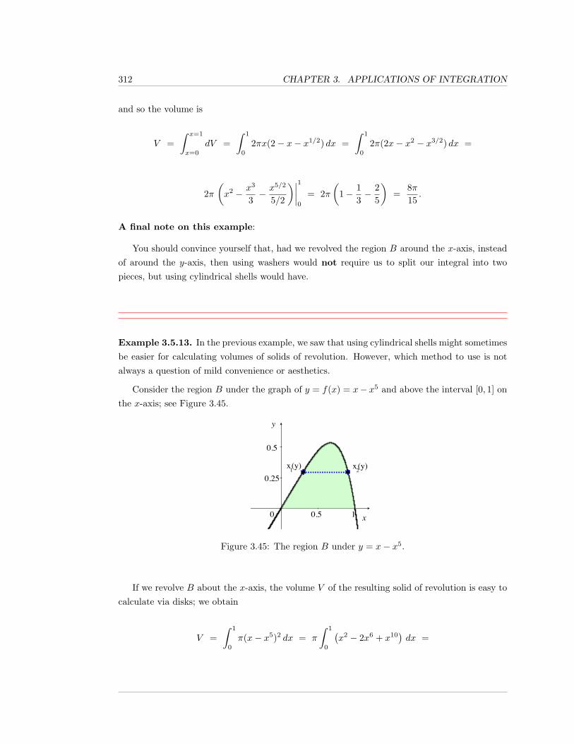
312 CHAPTER 3. APPLICATIONS OF INTEGRATION
and so the volume is
V =∫ x=1
x=0
dV =∫ 1
0
2πx(2− x− x1/2) dx =∫ 1
0
2π(2x− x2 − x3/2) dx =
2π(x2 − x3
3− x5/2
5/2
)∣∣∣∣10
= 2π(
1− 13− 2
5
)=
8π15.
A final note on this example:
You should convince yourself that, had we revolved the region B around the x-axis, insteadof around the y-axis, then using washers would not require us to split our integral into twopieces, but using cylindrical shells would have.
Example 3.5.13. In the previous example, we saw that using cylindrical shells might sometimesbe easier for calculating volumes of solids of revolution. However, which method to use is notalways a question of mild convenience or aesthetics.
Consider the region B under the graph of y = f(x) = x− x5 and above the interval [0, 1] onthe x-axis; see Figure 3.45.
-0.5 0 0.5 1
-0.25
0.25
0.5
x (y)1 x (y)2
Figure 3.45: The region B under y = x− x5.
If we revolve B about the x-axis, the volume V of the resulting solid of revolution is easy tocalculate via disks; we obtain
V =∫ 1
0
π(x− x5)2 dx = π
∫ 1
0
(x2 − 2x6 + x10
)dx =
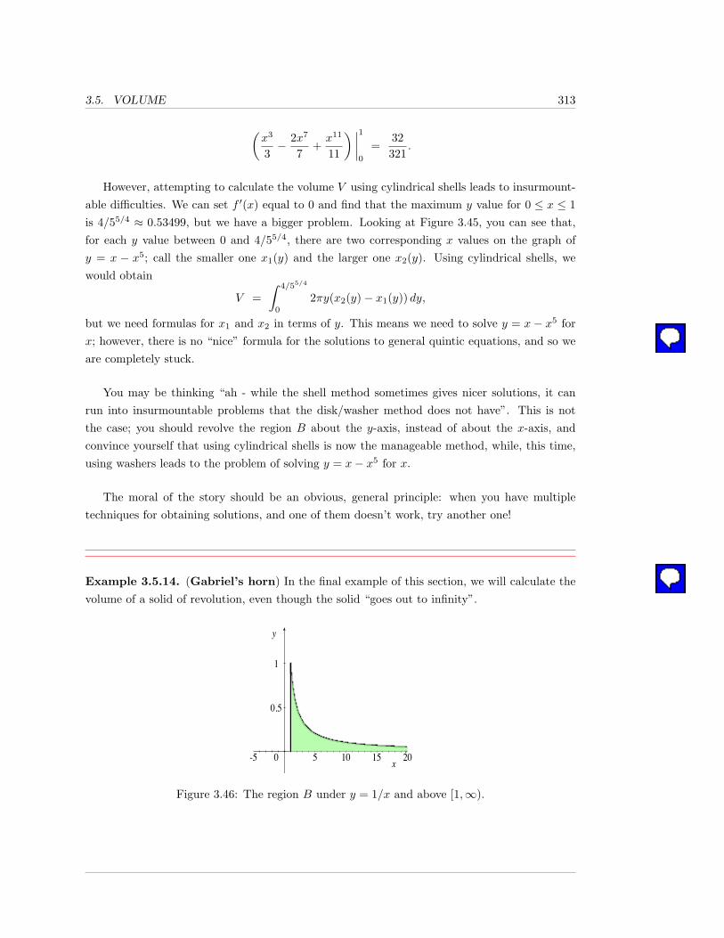
3.5. VOLUME 313
(x3
3− 2x7
7+x11
11
) ∣∣∣∣10
=32321
.
However, attempting to calculate the volume V using cylindrical shells leads to insurmount-able difficulties. We can set f ′(x) equal to 0 and find that the maximum y value for 0 ≤ x ≤ 1is 4/55/4 ≈ 0.53499, but we have a bigger problem. Looking at Figure 3.45, you can see that,for each y value between 0 and 4/55/4, there are two corresponding x values on the graph ofy = x − x5; call the smaller one x1(y) and the larger one x2(y). Using cylindrical shells, wewould obtain
V =∫ 4/55/4
0
2πy(x2(y)− x1(y)) dy,
but we need formulas for x1 and x2 in terms of y. This means we need to solve y = x− x5 forx; however, there is no “nice” formula for the solutions to general quintic equations, and so weare completely stuck.
You may be thinking “ah - while the shell method sometimes gives nicer solutions, it canrun into insurmountable problems that the disk/washer method does not have”. This is notthe case; you should revolve the region B about the y-axis, instead of about the x-axis, andconvince yourself that using cylindrical shells is now the manageable method, while, this time,using washers leads to the problem of solving y = x− x5 for x.
The moral of the story should be an obvious, general principle: when you have multipletechniques for obtaining solutions, and one of them doesn’t work, try another one!
Example 3.5.14. (Gabriel’s horn) In the final example of this section, we will calculate thevolume of a solid of revolution, even though the solid “goes out to infinity”.
-5 0 5 10 15 20
-0.5
0.5
1
Figure 3.46: The region B under y = 1/x and above [1,∞).
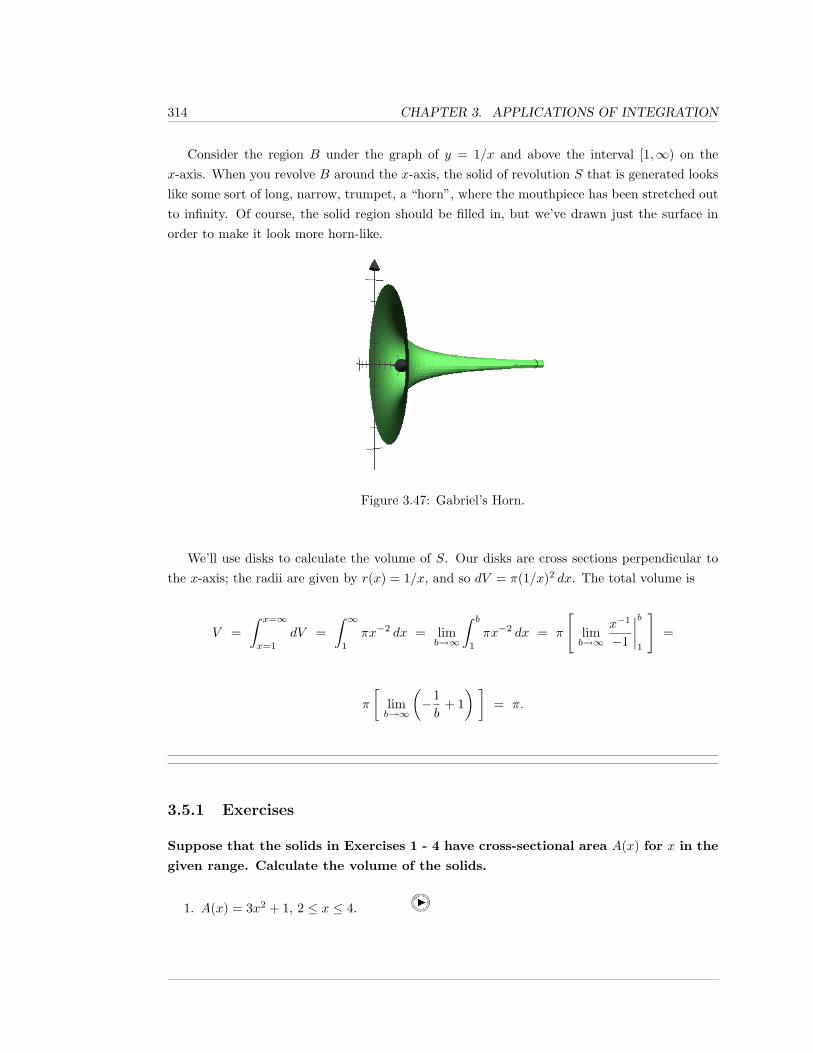
314 CHAPTER 3. APPLICATIONS OF INTEGRATION
Consider the region B under the graph of y = 1/x and above the interval [1,∞) on thex-axis. When you revolve B around the x-axis, the solid of revolution S that is generated lookslike some sort of long, narrow, trumpet, a “horn”, where the mouthpiece has been stretched outto infinity. Of course, the solid region should be filled in, but we’ve drawn just the surface inorder to make it look more horn-like.
Figure 3.47: Gabriel’s Horn.
We’ll use disks to calculate the volume of S. Our disks are cross sections perpendicular tothe x-axis; the radii are given by r(x) = 1/x, and so dV = π(1/x)2 dx. The total volume is
V =∫ x=∞
x=1
dV =∫ ∞
1
πx−2 dx = limb→∞
∫ b
1
πx−2 dx = π
[limb→∞
x−1
−1
∣∣∣∣b1
]=
π
[limb→∞
(−1b
+ 1) ]
= π.
3.5.1 Exercises
Suppose that the solids in Exercises 1 - 4 have cross-sectional area A(x) for x in the
given range. Calculate the volume of the solids.
1. A(x) = 3x2 + 1, 2 ≤ x ≤ 4.
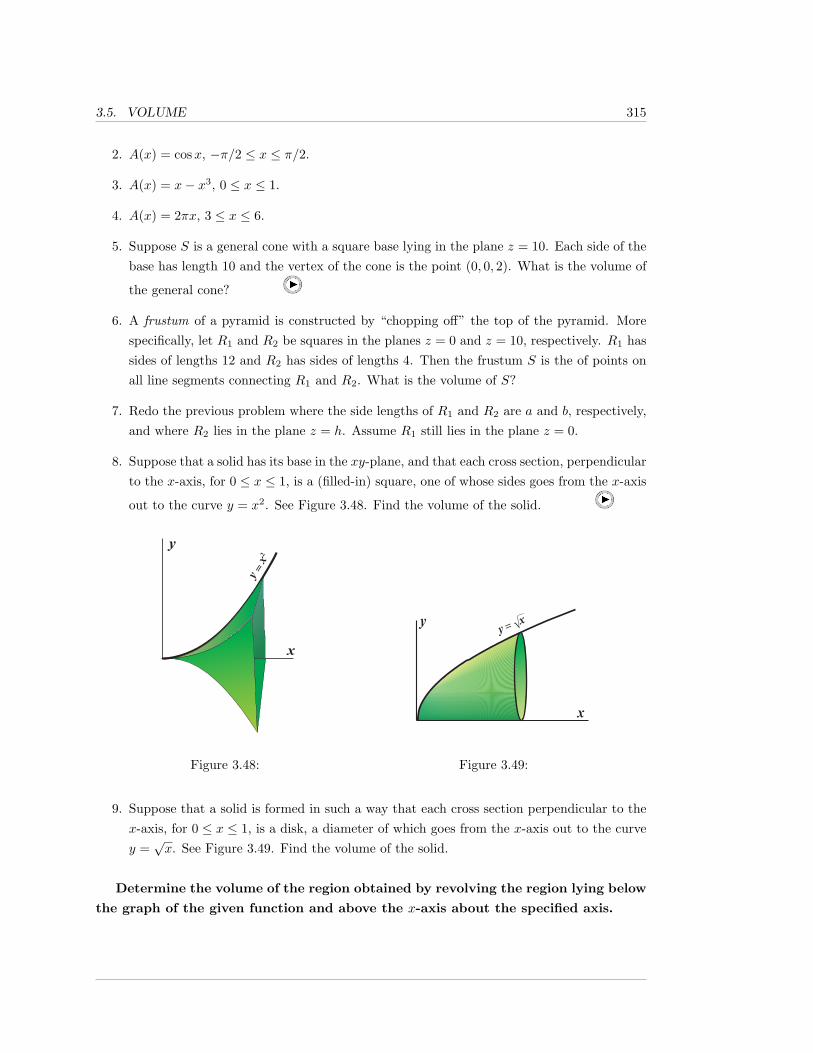
3.5. VOLUME 315
2. A(x) = cosx, −π/2 ≤ x ≤ π/2.
3. A(x) = x− x3, 0 ≤ x ≤ 1.
4. A(x) = 2πx, 3 ≤ x ≤ 6.
5. Suppose S is a general cone with a square base lying in the plane z = 10. Each side of thebase has length 10 and the vertex of the cone is the point (0, 0, 2). What is the volume of
the general cone?
6. A frustum of a pyramid is constructed by “chopping off” the top of the pyramid. Morespecifically, let R1 and R2 be squares in the planes z = 0 and z = 10, respectively. R1 hassides of lengths 12 and R2 has sides of lengths 4. Then the frustum S is the of points onall line segments connecting R1 and R2. What is the volume of S?
7. Redo the previous problem where the side lengths of R1 and R2 are a and b, respectively,and where R2 lies in the plane z = h. Assume R1 still lies in the plane z = 0.
8. Suppose that a solid has its base in the xy-plane, and that each cross section, perpendicularto the x-axis, for 0 ≤ x ≤ 1, is a (filled-in) square, one of whose sides goes from the x-axis
out to the curve y = x2. See Figure 3.48. Find the volume of the solid.
x
y
2y x=
x
y
2y x=
x
y 2y x=
x
y 2y x=
11 12
21 22Figure 3.48:
xy y �� x�
xy y �� x�
xy y �� x�
0
1
2Figure 3.49:
9. Suppose that a solid is formed in such a way that each cross section perpendicular to thex-axis, for 0 ≤ x ≤ 1, is a disk, a diameter of which goes from the x-axis out to the curvey =√x. See Figure 3.49. Find the volume of the solid.
Determine the volume of the region obtained by revolving the region lying below
the graph of the given function and above the x-axis about the specified axis.
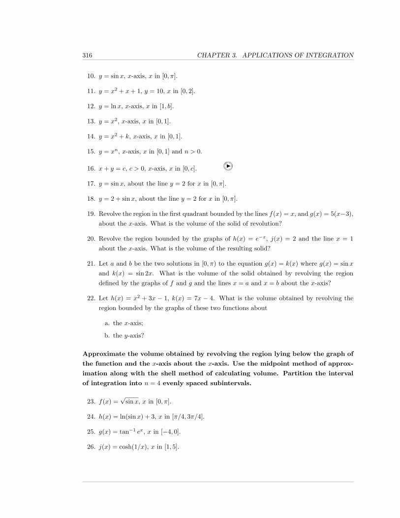
316 CHAPTER 3. APPLICATIONS OF INTEGRATION
10. y = sinx, x-axis, x in [0, π].
11. y = x2 + x+ 1, y = 10, x in [0, 2].
12. y = lnx, x-axis, x in [1, b].
13. y = x2, x-axis, x in [0, 1].
14. y = x2 + k, x-axis, x in [0, 1].
15. y = xn, x-axis, x in [0, 1] and n > 0.
16. x+ y = c, c > 0, x-axis, x in [0, c].
17. y = sinx, about the line y = 2 for x in [0, π].
18. y = 2 + sinx, about the line y = 2 for x in [0, π].
19. Revolve the region in the first quadrant bounded by the lines f(x) = x, and g(x) = 5(x−3),about the x-axis. What is the volume of the solid of revolution?
20. Revolve the region bounded by the graphs of h(x) = e−x, j(x) = 2 and the line x = 1about the x-axis. What is the volume of the resulting solid?
21. Let a and b be the two solutions in [0, π) to the equation g(x) = k(x) where g(x) = sinxand k(x) = sin 2x. What is the volume of the solid obtained by revolving the regiondefined by the graphs of f and g and the lines x = a and x = b about the x-axis?
22. Let h(x) = x2 + 3x − 1, k(x) = 7x − 4. What is the volume obtained by revolving theregion bounded by the graphs of these two functions about
a. the x-axis;
b. the y-axis?
Approximate the volume obtained by revolving the region lying below the graph of
the function and the x-axis about the x-axis. Use the midpoint method of approx-
imation along with the shell method of calculating volume. Partition the interval
of integration into n = 4 evenly spaced subintervals.
23. f(x) =√
sinx, x in [0, π].
24. h(x) = ln(sinx) + 3, x in [π/4, 3π/4].
25. g(x) = tan−1 ex, x in [−4, 0].
26. j(x) = cosh(1/x), x in [1, 5].
3.5. VOLUME 317
27. k(x) = ecos x, x in [0, π].
28. Let u(x) = xm and v(x) = xn where m > n ≥ 1. What is the volume obtained byrevolving the region bounded by the graphs of these two functions for x in [0, 1] about the
x-axis?
29. What is the volume obtained by revolving the region described in the previous problemabout the y-axis?
30. Suppose C is a right circular cone with its vertex at the origin, and with its circular basein the plane z = h. Assume the radius of the base is r. What is the average area of a crosssection parallel to the xy plane? Express your answer in terms of the volume of the coneand its height.
31. Suppose G is a general cone with vertex at the origin and with its base in the plane z = h.What is the average area of a cross section parallel to the xy plane?
32. Suppose that f ≥ 0 on the interval [0, b], that f is continuous, and that F is an anti-derivative of f . Prove that the volume obtained by revolving the region below the graph
of f(x) and above the x-axis about the y axis is V = −2π∫ b
0
F (x) dx.
33. Let f(x) =| sinx|x
for x > 1. Consider the solid obtained by revolving the region lyingbelow the graph of f and above the x-axis about the x-axis. Does this region have finitevolume? Hint: compare the volume to another region with a known volume.
34. Recall that the equationx2
a2+y2
b2= 1 defines an ellipse. Let R be the portion of the ellipse
lying in the upper-half plane, y > 0.
a. What is the volume obtained by revolving the region about the x-axis?
b. Set a = b in your result from part (a) and verify that this is the correct volumeformula for a sphere.
35. Let f(x) = coshx and g(x) = x + 1. Let a and b be the two x values where the graphsof the functions intersect. Calculate the volume obtained by revolving the area betweenthese two curves on the interval [a, b] about the x-axis.
36. Calculate the volume obtained by revolving the region in the previous problem about they-axis.
37. A torus in three dimensions can be obtained as follows. Let D be a disc in the xy planewith center (R, 0) and with radius r where r < R. Rotate the disc about the y-axis torealize a torus. For the next few problems, we refer to r as the inner radius and R as the
outer radius. Use the disc method to calculate the volume of this torus.
318 CHAPTER 3. APPLICATIONS OF INTEGRATION
38. Another way to construct a torus is to bend a cylinder until the top and bottom meet.The volume of the resultant torus is identical to that of the original cylinder. Use thesetup in the previous problem and calculate the volume of the torus by calculating thevolume of a cylinder.
39. Calculate the area obtained by revolving the region below the graph of y = sinx and abovethe x-axis on the interval x in [0, π] about the y-axis using:
a. The shell method;
b. The disk/washer method.
40. Suppose a torus shaped inner-tube is floating in a swimming pool. The inner radius is 4inches, and the outer radius is 18 inches. A portion of the inner tube is submerged belowthe water level. If the water level is half an inch, what is the volume of the submergedportion of the inner tube?
41. Suppose a spherical volleyball with radius 65 cm is floating in a pool so that the ball issubmerged up to 5 cm. What is the volume of the submerged portion of the ball?
42. Suppose an object with volume V is partially submerged in some fluid. Let Vs be thevolume of the submerged portion of the object. Suppose the density of the object is ρoand the density of the fluid is ρf . A basic result of fluid statics states that
VsV
=ρoρf.
Calculate the densities of the inner tube and volleyball mentioned in the previous twoproblems if the density of water 1 gm / cm3.
43. Suppose that the volleyball of radius 65 cm is again floating in water. The ratio of thevolumes of the submerged portion of the ball to the unsubmerged portion is 1 : 4. To whatdepth is the volleyball submerged?
44. Suppose we try to generalize Gabriel’s Horn.
a. Let f(x) = 1/xn and consider the solid formed by revolving the region lying belowthe graph of f and above the x-axis about the x-axis on the interval x in [1,∞). Doesthe volume exist when n ≥ 1? If so, what is the volume?
b. Does the volume exist when 0 < n < 1? If so, what is the volume?
45. Calculate the volume of the solid obtained by revolving the region bounded by the graphof y = 1/x, the line x = 1 and the line x = a where 0 < a < 1, about the y-axis. Does thisintegral converge as a→ 0?
3.5. VOLUME 319
46. Let R be the upper half of the disc centered at the origin with radius r. What is thevolume of the region obtained by revolving R about the line y = b where b ≥ r and b ≤ 0.
47. Let f(x) = cx2 and g(x) = c2√x where c > 0. Let Vc be the volume obtained by revolving
the region bounded by the graphs of f and g about the x-axis. What is Vc?
48. Calculate the volume of the region defined by revolving the region lying below the graphof y = sin(x2) and above the x-axis about the y-axis. Assume x in [0,
√π].
49. Suppose an annulus with inner radius r and outer radius R is situated in the plane z = π.The center of the annulus is the point (2, 700, π). What is the volume of the general conewith base the annulus and with a vertex at the origin?
50. Calculate the volume, if it exists, of the solid obtained by revolving the region lying belowthe graph of y = secx and above the x-axis about the x-axis on the interval [0, π/2].
51. Let g(x) = e−x2, x ∈ [0,∞). Calculate the volume, if it exists, of the region obtained by
revolving the region lying below the graph of g(x) and above the x-axis about the y-axis.
52. What is the volume obtained by revolving the region lying below the graph of y = e−x
and above the x-axis about the x-axis on the interval [0,∞)?
53. Consider the function
f(x) =
{e−x x ≥ 0ex x < 0
.
a. What is the volume obtained by revolving the region lying below the graph of f(x)and above the x-axis about the x-axis on the interval (−∞,∞)?
b. Use the disc method to try and calculate the volume obtained by revolving the regionbelow the graph of f(x) and above the x-axis around the y-axis for a ≤ y ≤ 1. Doesthis integral converge as a→ 0?
c. Try calculating the volume in part (b) using the shell method. Does your answerconcur with that in part (b)?
54. A right circular cone is obtained by revolving the region bounded by the curves y = mx,x = 0, and y = h, where m 6= 0, about the y-axis. What is the volume of the cone? Leaveyour answer in terms of m and h. Make sure to consider the case that m is negative.
55. Archimedes noted that if a right circular cone, a hemisphere, and a cylinder all have thesame heights and radii, then the ratios of their volumes is 1 : 2 : 3 in the order specifiedabove. Verify this claim. Observe that if we append a complete sphere to the tail of thissequence, the ratio pattern extends to 1 : 2 : 3 : 4.
320 CHAPTER 3. APPLICATIONS OF INTEGRATION
56. Suppose a regular n-gon (equilateral, equiangular and convex) is situated in the planez = h with its center on the z-axis. Recall that the apothem is the distance from thecenter of the polygon to the midpoint of one the sides.
a. Prove that the area of the n-gon with apothem a is given by Bn = a2n tanπ
n.
b. What is the volume, Vn, of the solid defined by the line segments connecting theorigin to the polygon?
c. Show that Bn → πa2 and Vn →πa2h
3as n→∞. Geometrically, why does this make
sense?
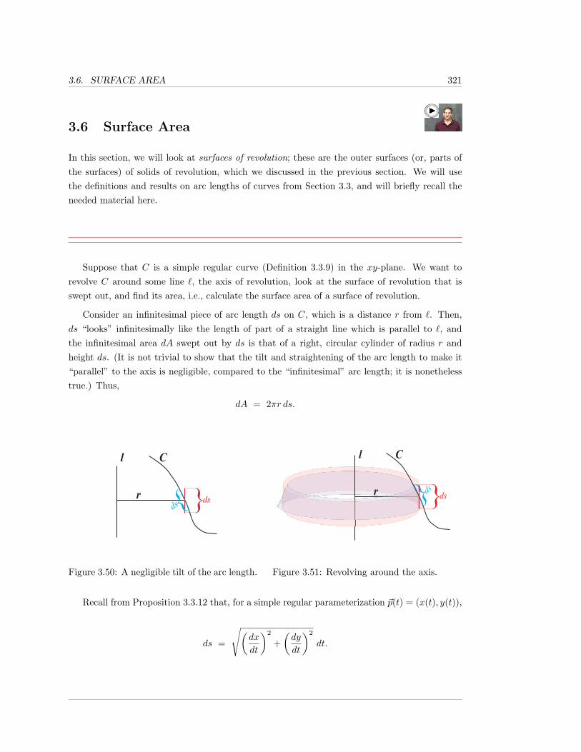
3.6. SURFACE AREA 321
3.6 Surface Area
In this section, we will look at surfaces of revolution; these are the outer surfaces (or, parts ofthe surfaces) of solids of revolution, which we discussed in the previous section. We will usethe definitions and results on arc lengths of curves from Section 3.3, and will briefly recall theneeded material here.
Suppose that C is a simple regular curve (Definition 3.3.9) in the xy-plane. We want torevolve C around some line `, the axis of revolution, look at the surface of revolution that isswept out, and find its area, i.e., calculate the surface area of a surface of revolution.
Consider an infinitesimal piece of arc length ds on C, which is a distance r from `. Then,ds “looks” infinitesimally like the length of part of a straight line which is parallel to `, andthe infinitesimal area dA swept out by ds is that of a right, circular cylinder of radius r andheight ds. (It is not trivial to show that the tilt and straightening of the arc length to make it“parallel” to the axis is negligible, compared to the “infinitesimal” arc length; it is nonethelesstrue.) Thus,
dA = 2πr ds.
}ds}dsl C
r}ds }ds
l Cr
Figure 3.50: A negligible tilt of the arc length.
}ds}dsl C
r
}ds }dsl C
r
Figure 3.51: Revolving around the axis.
Recall from Proposition 3.3.12 that, for a simple regular parameterization ~p(t) = (x(t), y(t)),
ds =
√(dx
dt
)2
+(dy
dt
)2
dt.
322 CHAPTER 3. APPLICATIONS OF INTEGRATION
Therefore, we have:
Proposition 3.6.1. If ~p(t) = (x(t), y(t)), for a ≤ t ≤ b, is a simple regular parameterizationof C, and r(t) equals the distance from ~p(t) to `, then the area of the surface of revolutiongenerated by revolving C around ` is
surface area =∫ t=b
t=a
dA =∫ t=b
t=a
2πr ds =∫ b
a
2πr(t)
√(dx
dt
)2
+(dy
dt
)2
dt.
As in Section 3.3, if we are given the curve C as part of the graph of a function y = f(x) orx = f(y), then ds can be written as
√1 +
(dy
dx
)2
dx or
√1 +
(dx
dy
)2
dy,
respectively; if you were using one of these forms for ds, then you would need to write the distanceto `, the “radius” r, in terms of x or y, respectively. Rather than rewrite Proposition 3.6.1 inevery conceivable form, we shall, instead, look at four specific examples.
We should remark at this point that, as with arc length integrals, the integrals/anti-derivativesthat arise in trying to calculate the areas of surfaces of revolution are usually ridiculously dif-ficult or impossible (to obtain as elementary functions). Of course, you can approximate theintegrals very closely by using numerical techniques from Section 2.6. The examples that we areabout to give are very special ones, for which we will be able to obtain exact areas.
Example 3.6.2. You may already know a/the formula for the surface area of a sphere of radiusR, but let’s calculate it as the area of a surface of revolution, and make sure that we get thewell-known result.
Consider the upper semi-circle C of radius R, centered at the origin in the xy-plane. Thissemi-circle has a simple regular parameterization given by
~p(t) = (x(t), y(t)) = (R cos t, R sin t), for 0 ≤ t ≤ π,
3.6. SURFACE AREA 323
and the sphere of radius R, centered at the origin, is the surface of revolution obtained byrevolving C around the x-axis. As we are revolving around the x-axis, r = r(t) is the y-coordinate on C, i.e., r = R sin t.
We calculate
ds =
√(dx
dt
)2
+(dy
dt
)2
dt =√
(−R sin t)2 + (R cos t)2dt = Rdt,
and
surface area of a sphere of radius R =∫ t=π
t=0
2πr ds =∫ π
0
2π(R sin t)Rdt =
2πR2(− cos t)∣∣∣π0
= 2πR2(− (−1)− (−1)
)= 4πR2,
which is what you may have learned in high school.
Remark 3.6.3. You may look at the formula V = 43πR
3 for the volume inside a sphere of radiusR and the formula A = 4πR2 for the surface area of the sphere, and notice that dV/dR = A. Isthis just a coincidence? No.
Just as we used integrals involving cylindrical shells, thickened cylinders, to calculate thevolumes of solids of revolution in Section 3.5, we could have used integrals involving sphericalshells, infinitesimally thickened spheres (remember: the sphere is just the surface, not the inside)to calculate the volume inside a sphere.
Let A(r) denote the surface area of a sphere of radius r. Then, consider the volume insidea sphere of radius R. For each r, where 0 ≤ r ≤ R, we can consider the infinitesimal volumeof the infinitesimally thickened sphere of radius r (with the same center as the big sphere); thisinfinitesimal volume is
dV = A(r) dr,
and the total volume inside the sphere of radius R is
V (R) =∫ R
0
A(r) dr.
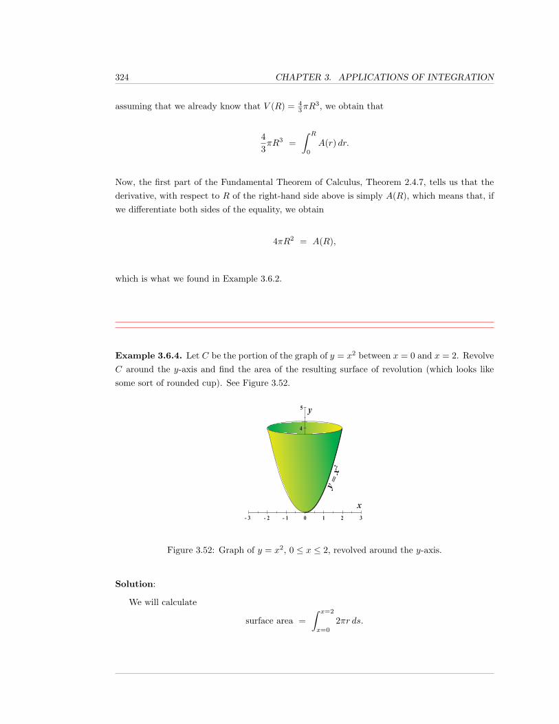
324 CHAPTER 3. APPLICATIONS OF INTEGRATION
assuming that we already know that V (R) = 43πR
3, we obtain that
43πR3 =
∫ R
0
A(r) dr.
Now, the first part of the Fundamental Theorem of Calculus, Theorem 2.4.7, tells us that thederivative, with respect to R of the right-hand side above is simply A(R), which means that, ifwe differentiate both sides of the equality, we obtain
4πR2 = A(R),
which is what we found in Example 3.6.2.
Example 3.6.4. Let C be the portion of the graph of y = x2 between x = 0 and x = 2. RevolveC around the y-axis and find the area of the resulting surface of revolution (which looks likesome sort of rounded cup). See Figure 3.52.
123
x- 1 1- 2 2- 3 3
45
0
y
2y x=
Figure 3.52: Graph of y = x2, 0 ≤ x ≤ 2, revolved around the y-axis.
Solution:
We will calculate
surface area =∫ x=2
x=0
2πr ds.
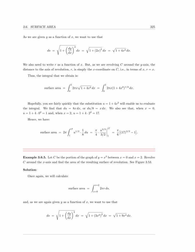
3.6. SURFACE AREA 325
As we are given y as a function of x, we want to use that
ds =
√1 +
(dy
dx
)2
dx =√
1 + (2x)2dx =
√1 + 4x2 dx.
We also need to write r as a function of x. But, as we are revolving C around the y-axis, thedistance to the axis of revolution, r, is simply the x-coordinate on C, i.e., in terms of x, r = x.
Thus, the integral that we obtain is:
surface area =∫ 2
0
2πx√
1 + 4x2 dx =∫ 2
0
2πx(1 + 4x2)1/2 dx.
Hopefully, you see fairly quickly that the substitution u = 1 + 4x2 will enable us to evaluatethe integral. We find that du = 8x dx, or du/8 = x dx. We also see that, when x = 0,u = 1 + 4 · 02 = 1 and, when x = 2, u = 1 + 4 · 22 = 17.
Hence, we have:
surface area = 2π∫ 17
1
u1/2 · 18du =
π
4· u
3/2
3/2
∣∣∣∣17
1
=π
6[(17)3/2 − 1
].
Example 3.6.5. Let C be the portion of the graph of y = x3 between x = 0 and x = 2. RevolveC around the x-axis and find the area of the resulting surface of revolution. See Figure 3.53.
Solution:
Once again, we will calculate
surface area =∫ x=2
x=0
2πr ds,
and, as we are again given y as a function of x, we want to use that
ds =
√1 +
(dy
dx
)2
dx =√
1 + (3x2)2dx =
√1 + 9x4 dx.
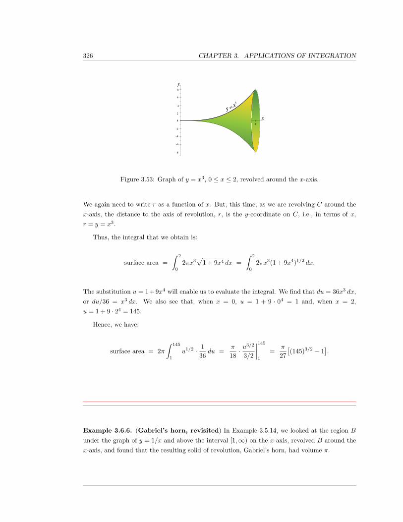
326 CHAPTER 3. APPLICATIONS OF INTEGRATION
x22- 2
- 4
4
- 6
6
- 8
8
0
y3y x=
1
Figure 3.53: Graph of y = x3, 0 ≤ x ≤ 2, revolved around the x-axis.
We again need to write r as a function of x. But, this time, as we are revolving C around thex-axis, the distance to the axis of revolution, r, is the y-coordinate on C, i.e., in terms of x,r = y = x3.
Thus, the integral that we obtain is:
surface area =∫ 2
0
2πx3√
1 + 9x4 dx =∫ 2
0
2πx3(1 + 9x4)1/2 dx.
The substitution u = 1 + 9x4 will enable us to evaluate the integral. We find that du = 36x3 dx,or du/36 = x3 dx. We also see that, when x = 0, u = 1 + 9 · 04 = 1 and, when x = 2,u = 1 + 9 · 24 = 145.
Hence, we have:
surface area = 2π∫ 145
1
u1/2 · 136du =
π
18· u
3/2
3/2
∣∣∣∣145
1
=π
27[(145)3/2 − 1
].
Example 3.6.6. (Gabriel’s horn, revisited) In Example 3.5.14, we looked at the region B
under the graph of y = 1/x and above the interval [1,∞) on the x-axis, revolved B around thex-axis, and found that the resulting solid of revolution, Gabriel’s horn, had volume π.
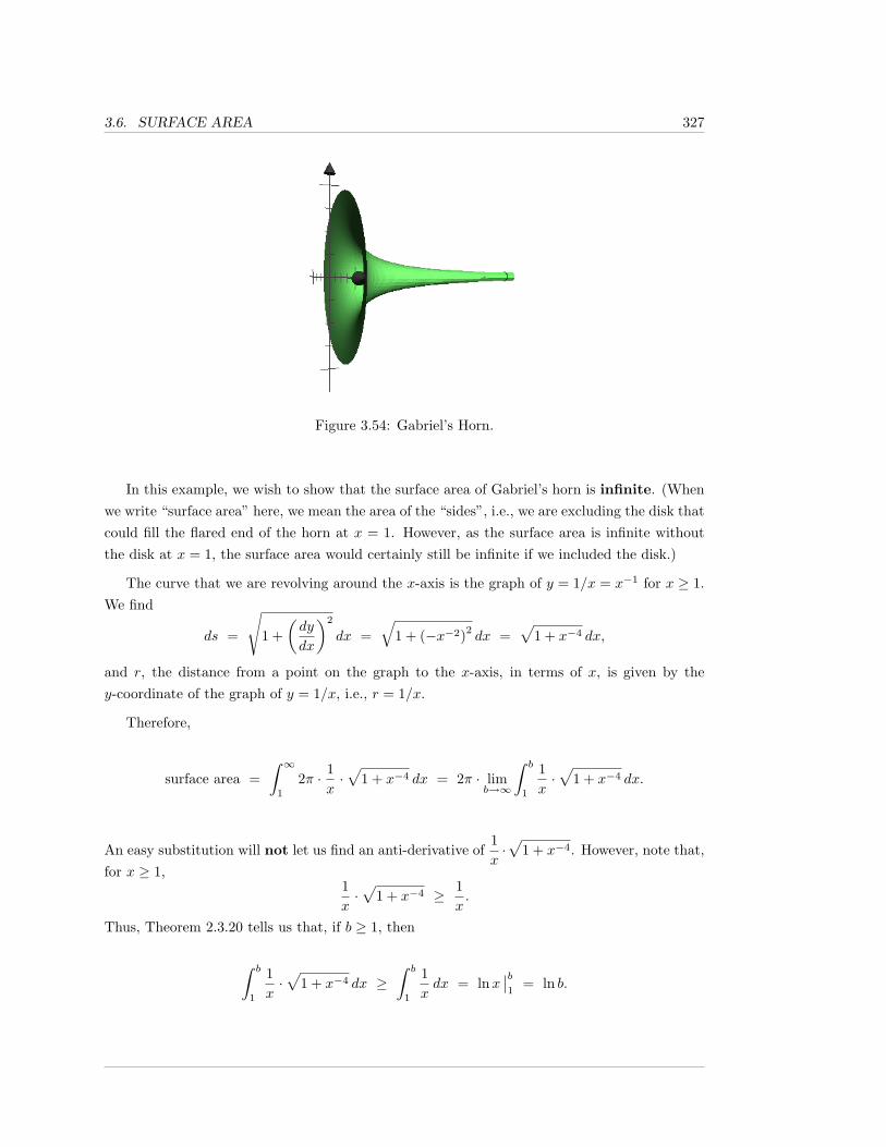
3.6. SURFACE AREA 327
Figure 3.54: Gabriel’s Horn.
In this example, we wish to show that the surface area of Gabriel’s horn is infinite. (Whenwe write “surface area” here, we mean the area of the “sides”, i.e., we are excluding the disk thatcould fill the flared end of the horn at x = 1. However, as the surface area is infinite withoutthe disk at x = 1, the surface area would certainly still be infinite if we included the disk.)
The curve that we are revolving around the x-axis is the graph of y = 1/x = x−1 for x ≥ 1.We find
ds =
√1 +
(dy
dx
)2
dx =√
1 + (−x−2)2dx =
√1 + x−4 dx,
and r, the distance from a point on the graph to the x-axis, in terms of x, is given by they-coordinate of the graph of y = 1/x, i.e., r = 1/x.
Therefore,
surface area =∫ ∞
1
2π · 1x·√
1 + x−4 dx = 2π · limb→∞
∫ b
1
1x·√
1 + x−4 dx.
An easy substitution will not let us find an anti-derivative of1x·√
1 + x−4. However, note that,for x ≥ 1,
1x·√
1 + x−4 ≥ 1x.
Thus, Theorem 2.3.20 tells us that, if b ≥ 1, then
∫ b
1
1x·√
1 + x−4 dx ≥∫ b
1
1xdx = lnx
∣∣b1
= ln b.
328 CHAPTER 3. APPLICATIONS OF INTEGRATION
As b goes to infinity, so does ln b, and this forces the larger quantity∫ b
11x ·√
1 + x−4 dx to go toinfinity also. We conclude:
surface area of Gabriel’s horn = 2π · ∞ = ∞.
Remark 3.6.7. The results of Example 3.5.14 and Example 3.6.6 tell us that Gabriel’s hornhas finite volume, but infinite surface area. These results are sometimes described as “you canfill Gabriel’s horn, but you can’t paint it”. The clever student then asks “What if you filled thehorn with paint? Wouldn’t that paint the surface?”.
This seeming contradiction is caused by a lack of precision in claiming that having infinitesurface area means that a surface can’t be painted. What is true is that having infinite surfacearea implies that the surface cannot be painted with a finite amount of paint, if we are requiredto have a uniformly thick layer of paint everywhere. However, if it were possible to havearbitrarily thin layers of paint, then the surface of Gabriel’s horn could be painted.
We’ll try to describe a similar problem, in which it’s hopefully easier to see what’s going on.
Suppose you took a cube that’s 1 foot long on each side, and you fill it with paint. Then,the volume of paint is finite; it’s 1 ft3. The surface area of the cube is the combined area of the6 sides, namely, 6 ft2.
Now, imagine chopping the cube in half by a cut which is parallel to two of the faces, whilesimultaneously sealing the two new exposed sides (or, you could think of inserting dividers intothe cube first, then chopping the cube in half). The total volume of paint in the two half-cubesis still 1 ft3, but now the surface area has gone up, because we created two new faces; the surfacearea is now 6 + 2 = 8 ft2.
Now, by making a cut parallel to the original cut, divide (and seal) one of the two half-cubesfrom above; the volume of paint remains 1 ft3, but we added two more faces, for a new surfacearea of 10 ft2. Imagine continuing this process indefinitely, each time, taking one of your smallesttwo pieces, and dividing it into two pieces by making a cut parallel to all of the other cuts. Thevolume of paint is always 1 ft3, but the surface area gets arbitrarily large or, in the limit, isinfinite.
Is there a contradiction here? No, but note that the layer of paint on the sides of the smallerand smaller pieces can’t be any thicker than the width of each piece, which is getting arbitrarysmall (close to zero).
3.6. SURFACE AREA 329
3.6.1 Exercises
Calculate the area of the surface obtained by revolving the graph of the function
about the x-axis. Recall that the notation x ∈ [a, b] means x takes on values in this
interval. In the first problem, for example, the portion of the graph of y = 3x + 4between x = 3 and x = 7 is being revolved.
1. y = 3x+ 4, x ∈ [3, 7].
2. y = sinx, x ∈ [0, π].
3. y = ex, x ∈ [0, π].
4. y = coshx, x ∈ [0, 1].
5. y =√x, x ∈ [0, 9].
6. y = sinhx, x ∈ [0, 10].
Calculate the area of the surface obtained by revolving the graph of the function
about the y-axis.
7. y = 2x− 3, x ∈ [4, 7].
8. y = 4x2, x ∈ [0, 6].
9. y = x1/3, x ∈ [1, 8].
10. y = x3, x ∈ [0, 2].
11. y = coshx, x ∈ [0, 4].
Calculate the area of the surface obtained by revolving the graph of the function
about the given axis.
12. y = 3x+ 13, x = 0, x ∈ [−4, 0].
13. y = 3x+ 1, x = 4, x ∈ [0, 4].
14. y = x2, y = 1, x ∈ [0, 1].
15. y = x2, x = 1, x ∈ [0, 1].
330 CHAPTER 3. APPLICATIONS OF INTEGRATION
16. y = x− 5, y = 3, x ∈ [5, 8].
17. y = mx+ b, m 6= 0, y = b, x ∈ [0, 1].
Approximate the areas of the surfaces obtained by revolving the graph of the func-
tion about the y-axis. Use the Midpoint Rule with n = 4 evenly spaced partitions.
18. y = lnx, x ∈ [1, 9].
19. y = x2 + 3x+ 5, x ∈ [0, 12].
20. y = x4, x ∈ [3.7].
21. y = x−2, x ∈ [4, 8].
22. y = tanhx, x ∈ [0, 4].
23. y =1
1 + x, x ∈ [0, 1].
24. Suppose that f(x) is a positive differentiable function. Argue that the surface area obtained
by revolving the graph of f(x) about the x-axis on the interval [a, b] is
A = 2π∫ b
a
f(x)√
1 + [f ′(x)]2 dx.
25. Given the setup in the previous problem, what is the surface area obtained by revolvingf(x) about the line y = y0? Assume f(x) > y0 for all x ∈ [a, b].
26. Suppose again that f(x) is a positive differentiable function. Argue that the surface areaobtained by revolving the graph of f(x) about the y-axis over the interval [a, b] is
A = 2π∫ b
a
x
√1 + [f ′(x)]2 dx.
Assume a > 0.
27. Given the setup in the previous problem, what is the surface area obtained by revolvingthe graph of f(x) about the line x = x0? Assume x0 < a.
28. a. What is the surface area obtained by revolving the line y = mx about the x-axis forx ∈ [0, a]?
3.6. SURFACE AREA 331
b. If the surface area function you obtained in part (a) is S(m), is S a continuousfunction of m? Is it differentiable?
29. Let a, b > 0. What is the area obtained by revolving the curve y = a√x+ b about the
x-axis for x ∈ [0, 1]?
30. Consider the torus obtained by revolving the circle (x − 2)2 + y2 = 1 about the y axis.Calculate the area of the torus by computing the area of the upper half of the torus andmultiplying by two.
31. a. What is the surface area obtained by revolving the line y = mx about the y-axis forx ∈ [0, a]?
b. If the surface area function you obtained in part (a) is S(m), is S a continuousfunction of m? Is it differentiable?
32. Consider the horizontal line segment in the xy-plane with end points (1, 3) and (2, 3).
a. Find a parameterization of the line segment.
b. Find the area of the surface obtained by revolving the segment about the y-axis.
c. What familiar shape is this? Check that your answer to part (b) is correct by calcu-lating the area using classical geometry.
33. Consider again the horizontal line segment in the xy-plane with end points (1, 3) and (2, 3).
a. Find the area of the surface obtained by revolving the segment about the y-axis.
b. What familiar shape is this? Check that your answer to part (a) is correct by calcu-lating the area using classical geometry.
34. Let C be a right circular cone obtained by revolving the line y = x about the y-axis.
Suppose that sand is poured into the cone.
a. Calculate the surface area of the sand in the cone as a function of y, the height ofthe sand in the cone. Include the circular base of the cone in your analysis.
b. If S(y) is the surface area of the sand in the cone, what is dS/dy?
35. Prove that the distance between a point (x1, y1) and the line y = mx is given by theequation
d =|y1 −mx1|√m2 + 1
.
36. Assume f(x) is a continuous function with f(x) > mx. Use the previous problem toderive an integral equation for the area obtained by revolving the graph of the function
f(x) about the line y = mx for x ∈ [a, c].
332 CHAPTER 3. APPLICATIONS OF INTEGRATION
37. Generalize the result in the previous problem. How does the equation for the surface area
change if the axis of rotation has the more general equation y = mx+ b?
38. Let θ be the angle the line y = mx makes with the x-axis. What is the surface area ofthe figure obtained by revolving the graph of f(x) about the line y = mx in terms of θ?Assume x ∈ [a, c]. Hint: no need to start from scratch. Use the previous problems andfind an equation relating m and θ.
39. With the notation of the previous problem, derive formulas for the surface area in thespecial cases. Assume that in all cases, the graph of f(x) lies on just one side of the axisof rotation. Assume x ∈ [a, c].
a. θ = 0.
b. θ = π/4.
c. θ = π/2.
40. In light of these results, justify the statement ”If a graph of a function lies in the firstquadrant and on one side of the line y = mx, then calculating the surface area obtainedby revolving the graph about y = mx is easy if we can calculate the area obtained byrevolving about the x-axis and y-axis.
41. What is the surface area of the region obtained by revolving the line segment y = 2x+ 4,x ∈ [3, 5] about the line y = 2x?
42. Let D be a the disk with radius 3 centered at the point (4, 2). Then the line y =12x cuts
the disc into two equal hemispheres. Calculate the surface area of the figure formed by
revolving the hemisphere about the line y =12x.
43. Let C be the circle defined by the equation (x − 3)2 + (y − 3)2 = 4. What is the surfacearea obtained by revolving the portion of C above the line y = x about the line y = x?
44. What is the surface area obtained by revolving the graph of the function h(x) = 4x − 2about the line y = 2x for x ∈ [1, 5]? What shape is this?
In Exercises 45-49, setup an integral to calculate the surface area of the region
obtained by rotating the graph of f(x) about the given line. Do not evaluate the
integral.
45. f(x) = ex, x ∈ [2, 5], y = 3x.
46. f(x) = cos2 x, x ∈ [−1, 0], y = x.
47. f(x) =x+ 2x+ 1
, x ∈ [2, 4], y = 2x.
3.6. SURFACE AREA 333
48. f(x) = x2 + 5x+ 1, x ∈ [0, 3], y =13x.
49. f(x) =√x+ 1, x ∈ [3, 8], y = 4x.
50. Suppose C is a piecewise simple regular curve. Formulate a reasonable equation for thevolume obtained by revolving C around an axis.
334 CHAPTER 3. APPLICATIONS OF INTEGRATION
3.7 Mass and Density
You are probably familiar with the concept of density, mass per volume. However, you mayhave never thought about “instantaneous density”. The issue is that objects may have differentdensities at different points. The density δ(P ) at a particular point P is defined by taking“small” chunks (rectangular solids) of the object around P , looking at the mass of such achunk divided by its volume, and taking the limit of this process as the volume of the chunkapproaches zero. A serious discussion of this limit belongs in multivariable Calculus, but thisinformal description should suffice for the applications in this section.
In terms of derivatives, we usually write that δ(P ) = dm/dV , i.e., that the density is theinstantaneous rate of change of the mass, with respect to volume. Or, in terms of infinitesimalquantities and differentials, the infinitesimal amount of mass dm at P is given by dm = δ(P ) dV ,where dV represents an infinitesimal volume in the object at P . Because it will help with thelater discussion, we will borrow notation and terminology from multivariable Calculus, and useundefined terms like “manageable type”, a “continuous function of three variables”, and an“integral over a solid region”, so that we can state:
Proposition 3.7.1. Suppose that a density function δ(P ) is continuous throughout a man-ageable solid region S. Then, an infinitesimal piece of mass at a point P in S is given bydm = δ(P ) dV , where dV is an infinitesimal volume in S around P , and the total mass ofS is the integral of δ, with respect to the volume, over the solid region S, i.e.,
mass of S =∫S
dm =∫S
δ(P ) dV.
Okay. Great. But now your question should be: How can we have a density which variesin a solid object, and still deal with the situation using single-variable Calculus? Actually, theproblem is not so bad – we just need to have situations in which the density varies only in asingle dimension. Okay. Fine. What does this mean?
One type of problem that we can handle is essentially what we discussed at the beginningof Section 3.5. We suppose that we have a solid region, S, in space, and that we know the areaA(x) of every cross-sectional slice of S which is perpendicular to the x-axis, and that the solidregion lies between the x cross sections where x = a and x = b, where a < b.
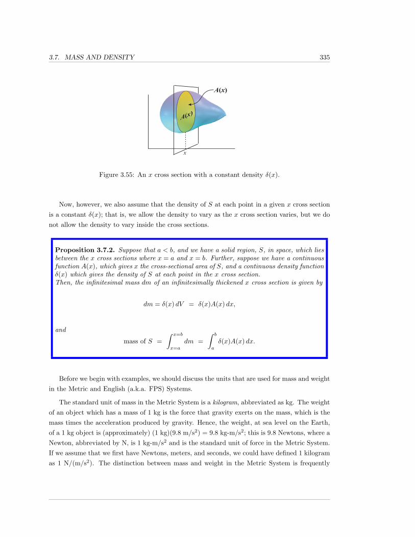
3.7. MASS AND DENSITY 335
A(x)A(x)
x
xixi-1si
¢xiFigure 3.55: An x cross section with a constant density δ(x).
Now, however, we also assume that the density of S at each point in a given x cross sectionis a constant δ(x); that is, we allow the density to vary as the x cross section varies, but we donot allow the density to vary inside the cross sections.
Proposition 3.7.2. Suppose that a < b, and we have a solid region, S, in space, which liesbetween the x cross sections where x = a and x = b. Further, suppose we have a continuousfunction A(x), which gives x the cross-sectional area of S, and a continuous density functionδ(x) which gives the density of S at each point in the x cross section.Then, the infinitesimal mass dm of an infinitesimally thickened x cross section is given by
dm = δ(x) dV = δ(x)A(x) dx,
and
mass of S =∫ x=b
x=a
dm =∫ b
a
δ(x)A(x) dx.
Before we begin with examples, we should discuss the units that are used for mass and weightin the Metric and English (a.k.a. FPS) Systems.
The standard unit of mass in the Metric System is a kilogram, abbreviated as kg. The weightof an object which has a mass of 1 kg is the force that gravity exerts on the mass, which is themass times the acceleration produced by gravity. Hence, the weight, at sea level on the Earth,of a 1 kg object is (approximately) (1 kg)(9.8 m/s2) = 9.8 kg-m/s2; this is 9.8 Newtons, where aNewton, abbreviated by N, is 1 kg-m/s2 and is the standard unit of force in the Metric System.If we assume that we first have Newtons, meters, and seconds, we could have defined 1 kilogramas 1 N/(m/s2). The distinction between mass and weight in the Metric System is frequently
336 CHAPTER 3. APPLICATIONS OF INTEGRATION
blurred in common speech. People often say something like “I weigh 70 kilos (kilograms)”. Theymean, of course, that their mass is 70 kg; there simply is no good verb form of the word “mass”.
You should be familiar with the standard unit of force in the English System; it’s the pound,abbreviated lb. Just as one 1 N/(m/s2) is called a kilogram, we give a name to 1 lb/(ft/s2); it iscalled a slug, which is not abbreviated. The acceleration produced by gravity, using English units,is (approximately) 32 ft/s2, and so, 1 slug, at sea level on the Earth, weighs (approximately) 32lb.
Example 3.7.3. Consider the sphere of radius R, centered at the origin, and let S be the solidregion contained inside the upper hemisphere, as in Example 3.5.6. Assume that all distancesare measured in meters, and that the solid region S is composed of some highly compressiblematerial, so that the lower portion of S is more dense than the upper part. Assume that thedensity of S at each point in a given z cross section is δ(z) = 1000(2R − z) kg/m3. Find themass m of S.
Solution:
As we saw in Example 3.5.6, the infinitesimal volume of a thickened z cross section of S isdV = π(R2 − z2) dz cubic meters. The infinitesimal mass of this thickened slice of S is
dm = δ(z) dV = 1000π(2R− z)(R2 − z2) dz kg,
and the total mass of S is
m =∫ z=R
z=0
dm =∫ R
0
1000π(2R− z)(R2 − z2) dz =
1000π∫ R
0
(2R3 −R2z − 2Rz2 + z3) dz = 1000π(
2R3z − R2 · z2
2− 2R · z
3
3+
z4
4
)∣∣∣∣R0
=
1000π(
13R4
12− 0
)=
13, 000πR4
12kilograms.
There is another situation in which we can find the mass of a solid by integrating a densityfunction which depends on only one variable. Suppose that we have a solid of revolution, S, as
3.7. MASS AND DENSITY 337
we discussed in Section 3.5, and that the density of the solid at any point P depends solely on thedistance r from the point P to the axis of revolution. Then, corresponding to finding volumesof solids of revolutions by using cylindrical shells, we can integrate to add up the infinitesimalamounts of mass of each cylindrical shell to produce the total mass
For instance, suppose that B is a region located in the first and/or fourth quadrant of thexy-plane, and we create a solid of revolution S by revolving B around the y-axis. Then, thedistance from any point P to the axis of revolution is simply the x-coordinate of P , and theinfinitesimal volume of a cylindrical shell is
dV = 2πxh(x) dx,
where the height function h(x) is determined by the shape of the region B. Now, if the densityat each point P in S depends only on the distance to the y-axis, then S has the same densityat each point in the cylindrical shell of radius x; this means that δ = δ(x), and the infinitesimalmass dm of the cylindrical shell of radius x is
dm = δ(x) dV = 2πxh(x)δ(x) dx.
Now, of course, we integrate to add up all of these infinitesimal blobs of mass.
Example 3.7.4. Recall Example 3.5.12, in which we looked at the curved triangular region B
in the xy-plane, which has part of the y-axis as its left edge, its top edge is given by y = 2− x,and its bottom curved edge is given by y =
√x. This region lies between x = 0 and x = 1. We
revolved B around the y-axis, generating a solid of revolution S.
Assume that all distances are measured in meters, and that, if P is a point in S and thedistance from P to the y-axis is r, then the density of S at P is 200(1 + r) kg/m3. Find thetotal mass of S.
Solution:
As we saw in Example 3.5.12, the infinitesimal volume of a cylindrical shell with radius r = x
is given by
dV = 2πrh dx = 2πx(2− x− x1/2) dx cubic meters.
As the radius of the shell is r = x, the density of S at each point in this shell is δ(x) = 200(1+x)
338 CHAPTER 3. APPLICATIONS OF INTEGRATION
kg/m3, and the infinitesimal mass of this shell is
dm = δ(x) dV = 200(1 + x) · 2πx(2− x− x1/2) dx kg.
Therefore, the total mass of S, in kilograms, is given by
m =∫ x=1
x=0
dm =∫ 1
0
400π(1 + x)x (2− x− x1/2) dx.
To calculate this integral, you “pull out” the 400π, multiply out (i.e., expand) the remainingterms, and use the Power Rule multiple times. We leave it as an exercise for you to verify thatthe result is
m =3340π
21kilograms.
There are two other “types” of densities that are commonly used, when the object in questionis essentially 1-dimensional, like a wire, or essentially 2-dimensional, like a thin metal plate (alamina); the corresponding densities are referred to as length-density, and area-density.
What is length-density?
Consider a thin straight wire. For many purposes (like ours), the wire is considered as a1-dimensional object, a line segment. Suppose that we lay out the wire along the x-axis, between0 and L, where L is the length of the wire. Then, for each x between 0 and L, we want thelength-density, δ`(x), to be the limit of the quotient obtained by taking the mass of a smalllength of the wire around x, divided by that small length. Thus, by definition of δ`(x), we wantthe infinitesimal amount of mass dm, at x, on the wire to be given by
dm = δ`(x) dx,
i.e., δ`(x) is defined to be dm/dx.
While it is standard to deal with length-densities as we did in the previous paragraph, it is,of course, true that a wire is actually a 3-dimensional solid object; it’s just that two of the wire’sdimensions are very small. If we think of the wire as having 3 dimensions, and think of usualdensity, then can we make sense of what length-density means? Yes.
3.7. MASS AND DENSITY 339
At each x-coordinate between 0 and L, the wire has a tiny x cross-sectional area A(x). Wesuppose, as we did earlier, that, in each x cross section, the density has a constant value δ(x).An infinitesimal piece of volume dV on the wire at x is given by dV = A(x) dx and, as eachpoint on the wire in the x cross section has density δ(x), the infinitesimal mass dm of this pieceis
dm = δ(x) dV = δ(x)A(x) dx.
Thus, if you wish to think in terms of the usual density of a 3-dimensional solid object, youuse the setup that we just discussed, and define length-density by δ`(x) = δ(x)A(x). Then, youonce again obtain that
dm = δ`(x) dx.
Proposition 3.7.5. Suppose that a < b, and we have an idealized 1-dimensional object(think of a thin wire), laid out along the x-axis, lying between x = a and x = b. Further,suppose we have a continuous length-density function δ`(x) for the object. Then, the in-finitesimal mass dm of an infinitesimal portion of the object is given by dm = δ`(x) dx,and
mass of the object =∫ x=b
x=a
dm =∫ b
a
δ`(x) dx.
Example 3.7.6. A wire has been stretched out along the x-axis. Its left end is at x = 0 and itsright end is at x = 4 feet. Suppose that the length-density of the wire is given by δ`(x) = e−x
slugs/ft.
What is the mass of the “left half” of the wire between x = 0 and x = 2 feet? What is themass of the “right half” of the wire between x = 2 and x = 4 feet? What is the x-coordinatexm of the point (the mass midpoint) such that half of the mass of the wire lies to left of xm andhalf of the mass lies to the right?
Solution:
The infinitesimal mass dm is simply
dm = δ`(x) dx = e−x dx slugs.
Using the substitution u = −x, it is easy to show that∫e−x dx = −e−x + C.
340 CHAPTER 3. APPLICATIONS OF INTEGRATION
Thus, the mass ML of the left half of the wire is
∫ x=2
x=0
dm =∫ 2
0
e−x dx = −e−x∣∣∣20
= −e−2 − (−e0) = 1− e−2 ≈ 0.8646647 slugs.
The mass MR of the right half of the wire is
∫ x=4
x=2
dm =∫ 4
2
e−x dx = −e−x∣∣∣42
= −e−4 − (−e−2) = e−2 − e−4 ≈ 0.1170196 slugs.
The mass midpoint, xm, is the point such that
∫ x=xm
x=0
dm =∫ x=4
x=xm
dm,
that is
∫ xm
0
e−x dx =∫ 4
xm
e−x dx, which yields − e−xm − (−1) = −e−4 − (−e−xm).
Thus, we need
1 + e−4 = 2e−xm , which gives us xm = ln(
21 + e−4
)≈ 0.6749973 feet.
Now we want to look at area-density. What is area-density?
In a similar way to how we dealt with length-density, if we have a lamina (a plane regionwhich has been thickened slightly, e.g., a thin sheet of metal), then we could think of the usual3-dimensional density, where one of the dimensions is very small. However, in analogy withwhat we did for thin wires, we typically just think of the area-density, δar(P ), at each point Pon our idealized 2-dimensional plate. Thus, an infinitesimal chunk of mass dm on the plate willbe given by dm = δar(P ) dA, where dA is an infinitesimal area. Of course, we still need to beable to reduce this to a one-variable problem.
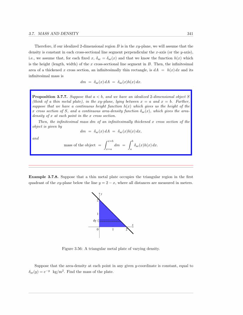
3.7. MASS AND DENSITY 341
Therefore, if our idealized 2-dimensional region B is in the xy-plane, we will assume that thedensity is constant in each cross-sectional line segment perpendicular the x-axis (or the y-axis),i.e., we assume that, for each fixed x, δar = δar(x) and that we know the function h(x) whichis the height (length, width) of the x cross-sectional line segment in B. Then, the infinitesimalarea of a thickened x cross section, an infinitesimally thin rectangle, is dA = h(x) dx and itsinfinitesimal mass is
dm = δar(x) dA = δar(x)h(x) dx.
Proposition 3.7.7. Suppose that a < b, and we have an idealized 2-dimensional object S(think of a thin metal plate), in the xy-plane, lying between x = a and x = b. Further,suppose that we have a continuous height function h(x) which gives us the height of thex cross section of S, and a continuous area-density function δar(x), which gives the area-density of x at each point in the x cross section.
Then, the infinitesimal mass dm of an infinitesimally thickened x cross section of theobject is given by
dm = δar(x) dA = δar(x)h(x) dx,
and
mass of the object =∫ x=b
x=a
dm =∫ b
a
δar(x)h(x) dx.
Example 3.7.8. Suppose that a thin metal plate occupies the triangular region in the firstquadrant of the xy-plane below the line y = 2− x, where all distances are measured in meters.
0 1 2
1
2
dy {
Figure 3.56: A triangular metal plate of varying density.
Suppose that the area-density at each point in any given y-coordinate is constant, equal toδar(y) = e−y kg/m2. Find the mass of the plate.
342 CHAPTER 3. APPLICATIONS OF INTEGRATION
Solution:
The length h(y) of an infinitesimally thin rectangle in the plate, at a given y-coordinate,is simply the corresponding x-coordinate on the line given by y = 2 − x, i.e., h(y) = 2 − y
meters. Hence, the infinitesimal area of the infinitesimally thin rectangle at each y-coordinateis dA = h(y) dy = (2− y) dy. The infinitesimal mass of this rectangle is
dm = δar(y) dA = e−y(2− y) dy
and, thus, the total mass of the plate is
mass of plate =∫ y=2
y=0
dm =∫ 2
0
e−y(2− y) dy =∫ 2
0
2e−y dy −∫ 2
0
ye−y dy kg.
This first integral is easy. We find
∫ 2
0
2e−y dy = −2e−y∣∣∣20
= −2e−2 − (−2e0) = 2− 2e−2.
We need to calculate the second integral and subtract. How do you calculate∫ 2
0ye−y dy? By
parts (Theorem 1.1.19).
Let’s calculate the indefinite integral, and then we’ll plug in the limits of integration. Letu = y and that leaves us with dv = e−y dy. Then, du = dy, v =
∫dv =
∫e−y dy = −e−y, and
Integration by Parts tells us that
∫ye−y dy =
∫u dv = uv −
∫v du = y(−e−y)−
∫−e−y dy = −ye−y − e−y + C.
Therefore, we obtain
∫ 2
0
ye−y dy = −ye−y − e−y∣∣∣20
= −e−y(y + 1)∣∣∣20
= −e−2(3) + 1 = 1− 3e−2,
and so,
mass of plate = 2− 2e−2 − (1− 3e−2) = 1 + e−2 kg.
3.7. MASS AND DENSITY 343
3.7.1 Exercises
Throughout the exercises, assume all information is given in standard metric units.
That is, mass is given in kilograms, time in seconds and lengths in meters.
1. Suppose that S is a rectangular solid in the first octant with 0 ≤ x ≤ 3, 0 ≤ y ≤ 6,and 0 ≤ z ≤ 5, and that the density is constant along each cross section parallel to the
xy-plane, with δ(z) = cosh z. Calculate the mass of S.
2. Suppose that S is a rectangular solid with sides parallel to the coordinate axes, whereeach cross section parallel to the xy plane has uniform density δ(z), and where a ≤ z ≤ b.Prove that the mass is given by m = A(z)
∫ baδ(z) dz. That is, show that area may be
factored out of the usual equation.
3. Suppose that S is a solid right circular cone, centered along the y-axis, with vertex at theorigin, and that the base lies in the plane y = 6 and has radius 4. Suppose that each crosssection parallel to the xz-plane has density δ(y) = 5y. Calculate the mass of S.
4. Generalize the result in the previous problem. Suppose S is a solid right circular cone,centered along the y axis, with height h, base radius r, vertex at the origin and densityfunction δ = δ(y). Give an integral for the mass of S.
5. Suppose that S is the solid ball centered at the origin with radius 9, and that the crosssections parallel to the yz-plane have density δ(x) = x2 + 1. Calculate the mass of S.
6. Suppose that S is the solid ellipsoid defined by the equation
x2
9+y2
4+z2
9= 1,
and that the cross sections parallel to the xz-plane have density δ(y) = 2y4 + y2 + 1.Calculate the mass of S.
In each of Exercises 7 through 14, calculate the mass of the solid of revolution S.
For each problem, assume the density function, δ, depends only on the distance r
from the point to the axis of revolution (as in Example 3.7.4).
344 CHAPTER 3. APPLICATIONS OF INTEGRATION
7. Let S be the solid obtained by revolving the first quadrant region below the curve y =√x
and above the interval [0, 4] about the y-axis, if δ(r) = r + 1.
8. S is the solid cone obtained by revolving the plane region bounded by the lines y = x,x = 0, y = 8 about the y-axis, with density function δ(r) = 1 + r3.
9. More generally, assume S is the solid cone obtained by revolving the plane region boundedby the lines y = mx, y = y0 > 0 and x = 0 with m > 0, about the y-axis, given a densityfunction δ(r). (Here, just give an appropriate integral for the mass.)
10. Consider the plane region B in the first quadrant bounded by the lines y = 5 and x = 4.Let S be the solid obtained by revolving B about the y-axis, with density function δ(r) =2 + cos(r2).
11. More generally, assume that B is the plane region in the first quadrant bounded by thelines y = h > 0, x = b > 0 and S is obtained by revolving B about the y-axis, given adensity function δ(r). (Here, just give an appropriate integral for the mass.)
12. Using the notation in the previous problem, what is the mass if h = 5, b = 7, but δ(r) ischanged to e−r?
13. Suppose B is the plane region in the first quadrant below the line y = 4, with 5 ≤ x ≤ 7.Let S be the solid obtained by revolving B about the y-axis, with δ(r) = ln r.
14. Consider the region in the first quadrant bounded by the curves y = 1.5x and y = cosπx,with x in [0, 1/3]. Let S be the region obtained by revolving this region about the y-axis,with δ(r) = r + 1.
In each of Exercises 15 through 19, you are given the length-density function, δ`(x),of an infinitesimally thin wire lying on the x-axis over a given interval. For each
problem, calculate (a) the total mass of the wire and (b) the mass midpoint (recall
Example 3.7.6). You may need to use technology to numerically approximate the
mass midpoint.
15. δ`(x) = x+ 7, 0 ≤ x ≤ 4.
16. δ`(x) =4
x2 − 9, 1 ≤ x ≤ 2.
17. δ`(x) = sinx, 0 ≤ x ≤ π/2.
18. δ`(x) = x lnx, 3 ≤ x ≤ 9.
19. δ`(x) = coshx, −1 ≤ x ≤ 1.
3.7. MASS AND DENSITY 345
20. Consider the following two quantities. C is the point in [a, b] such that∫ C
a
δ`(x) dx =∫ b
C
δ`(x) dx, and K =1
b− a
∫ b
a
δ`(x) dx. Briefly describe what C and K measure in
physical terms.
21. Suppose the length-density of a wire is δ`(x) = cex for x in [0, 10]. What is the massmidpoint?
22. Suppose the length-density of a wire is δ`(x) = ln(cx) for x in [1, c], where c > 1. Calculatethe mass midpoint in terms of c.
In each of Exercises 23 through 28, you are given a region B in the xy-plane, occupied
by a thin metal plate, and an area density function for the plate. If δar is given as
a function of x (resp. y), then δar gives the area-density of the plate at each point
in the x (resp. y) cross section. Calculate the mass of the metal plate.
23. Let B be the intersection of the disc centered at the origin with radius 3 and the firstquadrant, δar(x) = 3x+ 1.
24. B is the intersection of the disc centered at the origin with radius 5 and the first quadrant,δar(y) =
√1− y2 + 1.
25. Let B be the triangular region bounded by the coordinate axes and the line y = 2x − 6,δar(x) = x2 + 1.
26. B is the region in the first quadrant bounded by the curves y = cosx and y = sinx, with
0 ≤ x ≤ 4, and δar(x) = x+ 1.
27. B is the region in the first quadrant bounded by y =√x and x = 4, δar(y) = y3/2 + 2.
28. B is a triangle in the first quadrant with vertices (0, 0), (0, a), (b, 0). δar(y) = 1/(b+ 1).
29. Suppose B is triangle in the first quadrant with vertices (0, 0), (0, 2), (5, 0) with densityfunction δar(x) = cx2. What is c if the total mass is 25 kg?
The average density of a solid region with varying density is the total mass divided
by the total volume. Use this idea to answer each of Exercises 30 through 35.
30. Suppose S is a solid region where the density function of any plane parallel to the yz planeis given by δ(x). Suppose further that the area of each cross section parallel to the yz
346 CHAPTER 3. APPLICATIONS OF INTEGRATION
plane is A(x) and that a ≤ x ≤ b. Show that the average density of S is given by
average density =
∫ baδ(x)A(x) dx∫ baA(x) dx
.
31. Calculate the average density of the solid in Exercise 3.
32. Calculate the average density of the solid in Exercise 5.
33. Suppose that 0 ≤ a < b, that h(x) is continuous and positive, and that B is the planeregion under the graph of h(x) and above the interval [a, b] on the x-axis. Let S be thesolid obtained by revolving B about the y-axis. Suppose further that the density of theobject, δ(r), depends only on the distance from the y-axis. Show that the average densityof the solid is
average density =
∫ ba
2πxh(x)δ(x) dx∫ ba
2πxh(x) dx.
34. Calculate the average density of the solid in Exercise 7.
35. Calculate the average density of the solid in Exercise 8.
It’s common in physical applications for the density and mass of a region to evolve
over time. For example, we could be considering a rectangular solid initially con-
taining water, but where oil is added and mixed with the water. Over time, the
density and mass of the solid will evolve. In each of Exercises 36 through 39, the
density function is a function of time as well as position.
36. S is a rectangular solid with sides parallel to the coordinate planes, with −2 ≤ x ≤ 4,3 ≤ y ≤ 6, and 7 ≤ z ≤ 9. The density function δ(x, t) of a cross section parallel to the yzplane at time t is δ(x, t) = (t− 3)2ex.
a. Calculate m(t), the mass of the solid at time t.
b. Calculate dm/dt.
c. Assume t > 0. Is there a finite time when the mass is minimal?
37. Suppose S is a spherical ball centered at the origin with radius 3 and that the density
function is δ(r, t) =r + 1t
, where r is the distance between a point in the interior of theball and the origin. Assume t > 0.
a. Calculate m(t), the mass of the ball at time t.
3.7. MASS AND DENSITY 347
b. Calculate dm/dt.
38. In the previous problem, what is the average mass of the ball between times t = 2 andt = 5?
39. Suppose B is the region in the first quadrant bounded by the graph of ex and y = 9. LetS be the solid region obtained by revolving B about the y-axis. Suppose the density of anx cross section of S is given by δ(x, t) = tx+ t2 + 1. What is m(t)?
In the chapter, we saw that there was a special formula for calculating the mass of a
3-dimensional object when the density at a point depends on the distance between
the point and an axis. A similar formula exists in 2 dimensions. Suppose B is a
annulus or a disc in the xy-plane bounded by r = r0 and r = r1 and that the area-
density function, δ(r), depends only on the distance between a point on the surface
and the origin. Then the total mass is
mass = 2π∫ r1
r0
rδ(r) dr.
Use this formula to calculate the mass of the surface in each of Exercises 40 through
43.
40. B is a disk with radius 3 centered at the origin and with density function δ(r) = 3r + 1.
41. B is a disk with radius 5 centered at the origin with density function δ(r) =r + 2r + 1
.
42. B is an annulus centered at the origin bounded by circles of radii 4 and 7. δ(r) = 1/r.
43. B is an annulus centered at the origin bounded by circles of radii 2 and 6. δ(r) = 4er2.
348 CHAPTER 3. APPLICATIONS OF INTEGRATION
3.8 Centers of Massand Moments
We frequently discuss objects as though they are located at specific points. Of course, objects inreal life exist at an infinite number of points in space. When we state that an object of mass mis located at a point P , we are frequently thinking of an idealized “point-mass”: an imaginaryobject which occupies a single point in space at any given time.
However, the idealized notion of a point-mass is clearly unsatisfactory for many applications.For instance, the magnitude of the gravitational force between objects with masses M and m,is F = GMm/r2, where G is the universal gravitational constant and r is usually described asbeing the “distance between the two objects”. What is meant by this “distance”, when eachobject occupies an infinite number of points in space?
The answer is that the “distance” means the distancebetween the centers of mass of the two objects. Given anobject, or collection of objects, of (total) mass M , the centerof mass is a point P in space such that, in many physicalproblems, the object(s) can be treated as a point-mass, withmass M , located at the point P . If you were trying to bal-
ance a rigid wire or metal plate on your finger, the center of mass is where you would place yourfinger. If two children want to balance on a see-saw, the center of mass is the point where thebase (fulcrum) of the see-saw needs to be.
Note that the center of mass of an object need not actually be located at a point on theobject. Perhaps the easiest example of this is a uniformly dense annulus: think of a thin metaldisk with a smaller disk removed from its center; by symmetry, the center of mass is located atthe center of the annulus, but that part has been removed. What this means is that there is noplace where you could place your finger in order to balance an annulus. Hopefully, this seemsintuitively clear.
For a solid object, the center of mass can be determined, in principle, via integration, fromthe shape and density function (Section 3.7) of the object. For an object with constant density,the center of mass is also known as the centroid of the object.
In order to discuss how integration can be used to find centers of mass of objects, we firstneed to understand what happens for a finite number of point-masses. We shall describe this,and then define the center of mass.
The discussion of the center of mass is most natural using the language of vectors, which welooked at in Section 3.3, and for which there’s a quick summary in Appendix A. We shall use
3.8. CENTERS OF MASS AND MOMENTS 349
vectors now, but we shall also describe the situation later for wires and thin plates, and there weshall not refer to vectors. Our treatment follows that in the excellent volumes of The FeymanLectures on Physics, [1].
Suppose that we have n point-masses, whose masses are constants m1, . . . ,mn (not all zero),and the masses are moving in space (or in a plane, or in a line). Let ~ri = ~ri(t) denote theposition of the mass mi, for i = 1, . . . , n, at time t. (In other places, we have used ~p to denoteposition; it is standard in our current situation to use ~r, for radial vector.)
Suppose now that we have a force ~Fi = ~Fi(t) acting on each mass mi, and that ~Fi is the onlyforce acting on mi. Then, the vector form of Newton’s 2nd Law of Motion tells us that the netforce acting on an object (of constant mass) is the mass times the acceleration of the object,i.e.,
~Fi = mid2~ridt2
.
Now suppose that we think of all of the masses together as one object, possibly becausethey’re very close together, but possibly not. Then, the total mass of the new “object” isM =
∑ni=1mi, and the net force acting on the object is ~F =
∑ni=1
~Fi. We want to be able toapply Newton’s 2nd Law to the collective mass M ; that is, we want that ~F is equal to the massM times the acceleration. But what is this “acceleration” the acceleration of? Acceleration is,of course, the second derivative of position, with respect to time, but what position do we takethe second derivative of?
Using that the masses mi are constant, so that M is also constant, we have
~F =n∑i=1
~Fi =n∑i=1
d2(mi~ri)dt2
= Md2[(∑n
i=1mi~ri)/M]
dt2.
Therefore, if we define a position vector
~rcm = ~rcm(t) =
n∑i=1
mi~ri
M=
n∑i=1
mi~ri
n∑i=1
mi
,
then we obtain that~F = M
d2~rcm
dt2. (3.2)
350 CHAPTER 3. APPLICATIONS OF INTEGRATION
Hence, we make the following definition:
Definition 3.8.1. The center of mass of a collection/system of objects with massesm1, . . . ,mn at positions ~r1, . . . , ~rn, respectively, is the point
~rcm =
n∑i=1
mi~ri
n∑i=1
mi
.
If we let ~ri = (xi, yi, zi), then we find that
x = x-coordinate of the center of mass =
(n∑i=1
mixi
)/(n∑i=1
mi
);
y = y-coordinate of the center of mass =
(n∑i=1
miyi
)/(n∑i=1
mi
);
z = z-coordinate of the center of mass =
(n∑i=1
mizi
)/(n∑i=1
mi
).
The quantity M =∑ni=1mi is the total mass of the system. The quantities
∑ni=1mixi,∑n
i=1miyi, and∑ni=1mizi are referred to by various terms involving the word moment;
we shall refer to them as the x-, y-, and z-components, respectively, of the mass-moment about the origin. In fact, as we shall consider only mass-moment about onlythe origin, we will usually write simply the x-, y-, and z-components of the moment.
Different sources also use different notations for the components of the moment. Weshall try to avoid confusion; if M is the total mass, then we write Mx, My, and Mz for thex-, y-, and z-components of the moment, respectively.
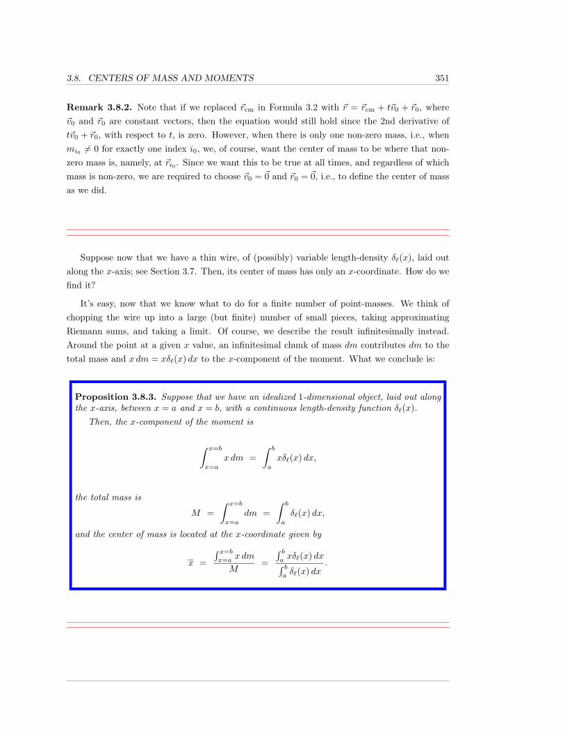
3.8. CENTERS OF MASS AND MOMENTS 351
Remark 3.8.2. Note that if we replaced ~rcm in Formula 3.2 with ~r = ~rcm + t~v0 + ~r0, where~v0 and ~r0 are constant vectors, then the equation would still hold since the 2nd derivative oft~v0 + ~r0, with respect to t, is zero. However, when there is only one non-zero mass, i.e., whenmi0 6= 0 for exactly one index i0, we, of course, want the center of mass to be where that non-zero mass is, namely, at ~ri0 . Since we want this to be true at all times, and regardless of whichmass is non-zero, we are required to choose ~v0 = ~0 and ~r0 = ~0, i.e., to define the center of massas we did.
Suppose now that we have a thin wire, of (possibly) variable length-density δ`(x), laid outalong the x-axis; see Section 3.7. Then, its center of mass has only an x-coordinate. How do wefind it?
It’s easy, now that we know what to do for a finite number of point-masses. We think ofchopping the wire up into a large (but finite) number of small pieces, taking approximatingRiemann sums, and taking a limit. Of course, we describe the result infinitesimally instead.Around the point at a given x value, an infinitesimal chunk of mass dm contributes dm to thetotal mass and x dm = xδ`(x) dx to the x-component of the moment. What we conclude is:
Proposition 3.8.3. Suppose that we have an idealized 1-dimensional object, laid out alongthe x-axis, between x = a and x = b, with a continuous length-density function δ`(x).
Then, the x-component of the moment is
∫ x=b
x=a
x dm =∫ b
a
xδ`(x) dx,
the total mass is
M =∫ x=b
x=a
dm =∫ b
a
δ`(x) dx,
and the center of mass is located at the x-coordinate given by
x =
∫ x=b
x=ax dm
M=
∫ baxδ`(x) dx∫ baδ`(x) dx
.
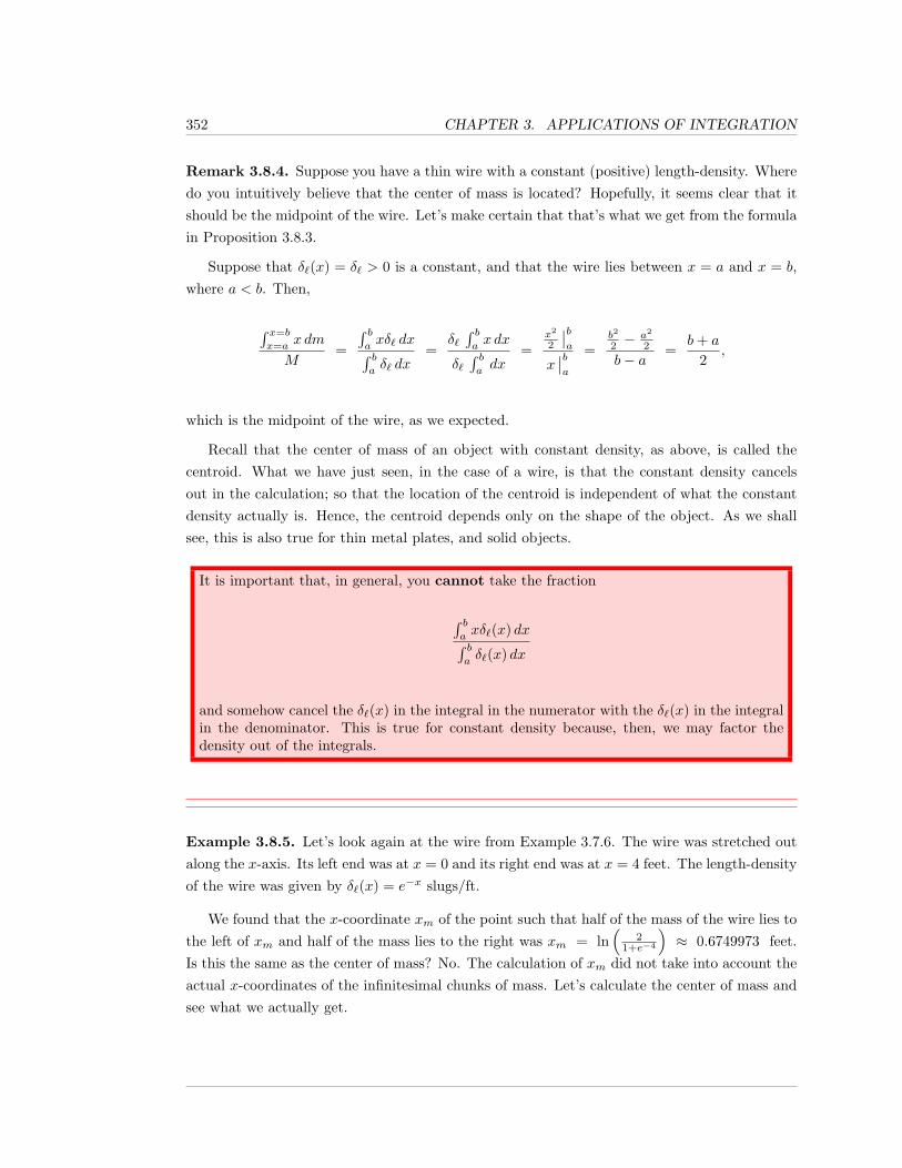
352 CHAPTER 3. APPLICATIONS OF INTEGRATION
Remark 3.8.4. Suppose you have a thin wire with a constant (positive) length-density. Wheredo you intuitively believe that the center of mass is located? Hopefully, it seems clear that itshould be the midpoint of the wire. Let’s make certain that that’s what we get from the formulain Proposition 3.8.3.
Suppose that δ`(x) = δ` > 0 is a constant, and that the wire lies between x = a and x = b,where a < b. Then,
∫ x=b
x=ax dm
M=
∫ baxδ` dx∫ baδ` dx
=δ`∫ bax dx
δ`∫ badx
=x2
2
∣∣ba
x∣∣ba
=b2
2 −a2
2
b− a=
b+ a
2,
which is the midpoint of the wire, as we expected.
Recall that the center of mass of an object with constant density, as above, is called thecentroid. What we have just seen, in the case of a wire, is that the constant density cancelsout in the calculation; so that the location of the centroid is independent of what the constantdensity actually is. Hence, the centroid depends only on the shape of the object. As we shallsee, this is also true for thin metal plates, and solid objects.
It is important that, in general, you cannot take the fraction
∫ baxδ`(x) dx∫ baδ`(x) dx
and somehow cancel the δ`(x) in the integral in the numerator with the δ`(x) in the integralin the denominator. This is true for constant density because, then, we may factor thedensity out of the integrals.
Example 3.8.5. Let’s look again at the wire from Example 3.7.6. The wire was stretched outalong the x-axis. Its left end was at x = 0 and its right end was at x = 4 feet. The length-densityof the wire was given by δ`(x) = e−x slugs/ft.
We found that the x-coordinate xm of the point such that half of the mass of the wire lies tothe left of xm and half of the mass lies to the right was xm = ln
(2
1+e−4
)≈ 0.6749973 feet.
Is this the same as the center of mass? No. The calculation of xm did not take into account theactual x-coordinates of the infinitesimal chunks of mass. Let’s calculate the center of mass andsee what we actually get.
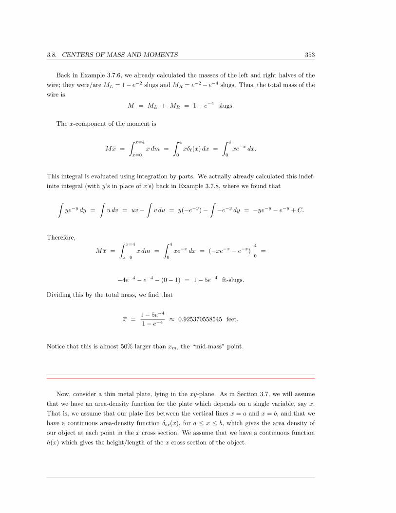
3.8. CENTERS OF MASS AND MOMENTS 353
Back in Example 3.7.6, we already calculated the masses of the left and right halves of thewire; they were/are ML = 1− e−2 slugs and MR = e−2− e−4 slugs. Thus, the total mass of thewire is
M = ML + MR = 1− e−4 slugs.
The x-component of the moment is
Mx =∫ x=4
x=0
x dm =∫ 4
0
xδ`(x) dx =∫ 4
0
xe−x dx.
This integral is evaluated using integration by parts. We actually already calculated this indef-inite integral (with y’s in place of x’s) back in Example 3.7.8, where we found that
∫ye−y dy =
∫u dv = uv −
∫v du = y(−e−y)−
∫−e−y dy = −ye−y − e−y + C.
Therefore,
Mx =∫ x=4
x=0
x dm =∫ 4
0
xe−x dx = (−xe−x − e−x)∣∣∣40
=
−4e−4 − e−4 − (0− 1) = 1− 5e−4 ft-slugs.
Dividing this by the total mass, we find that
x =1− 5e−4
1− e−4≈ 0.925370558545 feet.
Notice that this is almost 50% larger than xm, the “mid-mass” point.
Now, consider a thin metal plate, lying in the xy-plane. As in Section 3.7, we will assumethat we have an area-density function for the plate which depends on a single variable, say x.That is, we assume that our plate lies between the vertical lines x = a and x = b, and that wehave a continuous area-density function δar(x), for a ≤ x ≤ b, which gives the area density ofour object at each point in the x cross section. We assume that we have a continuous functionh(x) which gives the height/length of the x cross section of the object.
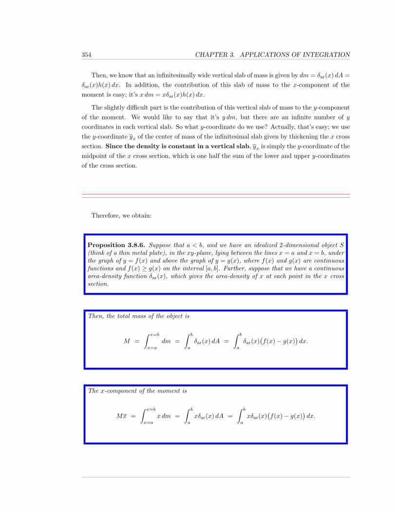
354 CHAPTER 3. APPLICATIONS OF INTEGRATION
Then, we know that an infinitesimally wide vertical slab of mass is given by dm = δar(x) dA =δar(x)h(x) dx. In addition, the contribution of this slab of mass to the x-component of themoment is easy; it’s x dm = xδar(x)h(x) dx.
The slightly difficult part is the contribution of this vertical slab of mass to the y-componentof the moment. We would like to say that it’s y dm, but there are an infinite number of ycoordinates in each vertical slab. So what y-coordinate do we use? Actually, that’s easy; we usethe y-coordinate yx of the center of mass of the infinitesimal slab given by thickening the x crosssection. Since the density is constant in a vertical slab, yx is simply the y-coordinate of themidpoint of the x cross section, which is one half the sum of the lower and upper y-coordinatesof the cross section.
Therefore, we obtain:
Proposition 3.8.6. Suppose that a < b, and we have an idealized 2-dimensional object S(think of a thin metal plate), in the xy-plane, lying between the lines x = a and x = b, underthe graph of y = f(x) and above the graph of y = g(x), where f(x) and g(x) are continuousfunctions and f(x) ≥ g(x) on the interval [a, b]. Further, suppose that we have a continuousarea-density function δar(x), which gives the area-density of x at each point in the x crosssection.
Then, the total mass of the object is
M =∫ x=b
x=a
dm =∫ b
a
δar(x) dA =∫ b
a
δar(x)(f(x)− g(x)
)dx.
The x-component of the moment is
Mx =∫ x=b
x=a
x dm =∫ b
a
xδar(x) dA =∫ b
a
xδar(x)(f(x)− g(x)
)dx.
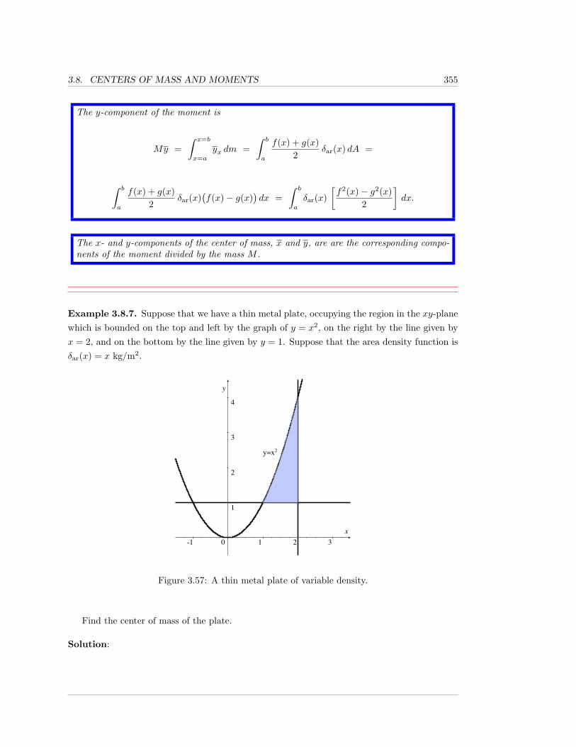
3.8. CENTERS OF MASS AND MOMENTS 355
The y-component of the moment is
My =∫ x=b
x=a
yx dm =∫ b
a
f(x) + g(x)2
δar(x) dA =
∫ b
a
f(x) + g(x)2
δar(x)(f(x)− g(x)
)dx =
∫ b
a
δar(x)[f2(x)− g2(x)
2
]dx.
The x- and y-components of the center of mass, x and y, are are the corresponding compo-nents of the moment divided by the mass M .
Example 3.8.7. Suppose that we have a thin metal plate, occupying the region in the xy-planewhich is bounded on the top and left by the graph of y = x2, on the right by the line given byx = 2, and on the bottom by the line given by y = 1. Suppose that the area density function isδar(x) = x kg/m2.
-1 0 1 2 3
1
2
3
4
y=x2
Figure 3.57: A thin metal plate of variable density.
Find the center of mass of the plate.
Solution:
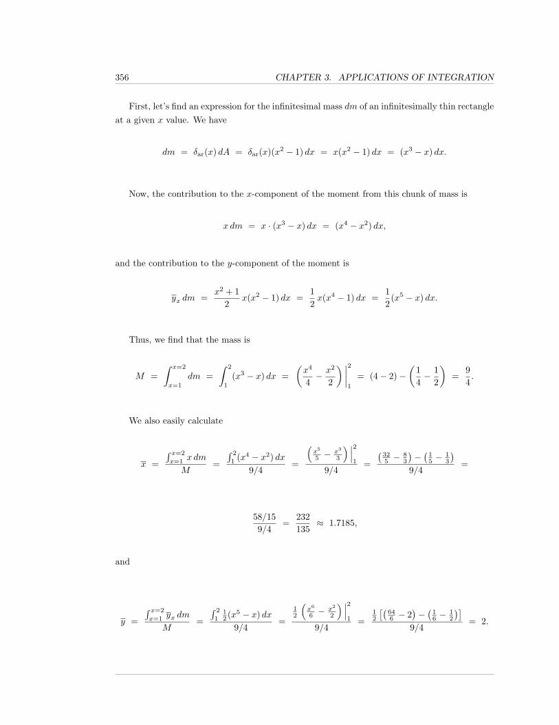
356 CHAPTER 3. APPLICATIONS OF INTEGRATION
First, let’s find an expression for the infinitesimal mass dm of an infinitesimally thin rectangleat a given x value. We have
dm = δar(x) dA = δar(x)(x2 − 1) dx = x(x2 − 1) dx = (x3 − x) dx.
Now, the contribution to the x-component of the moment from this chunk of mass is
x dm = x · (x3 − x) dx = (x4 − x2) dx,
and the contribution to the y-component of the moment is
yx dm =x2 + 1
2x(x2 − 1) dx =
12x(x4 − 1) dx =
12
(x5 − x) dx.
Thus, we find that the mass is
M =∫ x=2
x=1
dm =∫ 2
1
(x3 − x) dx =(x4
4− x2
2
) ∣∣∣∣21
= (4− 2)−(
14− 1
2
)=
94.
We also easily calculate
x =
∫ x=2
x=1x dm
M=
∫ 2
1(x4 − x2) dx
9/4=
(x5
5 −x3
3
) ∣∣∣21
9/4=
(325 −
83
)−(
15 −
13
)9/4
=
58/159/4
=232135
≈ 1.7185,
and
y =
∫ x=2
x=1yx dm
M=
∫ 2
112 (x5 − x) dx
9/4=
12
(x6
6 −x2
2
) ∣∣∣21
9/4=
12
[(646 − 2
)−(
16 −
12
)]9/4
= 2.
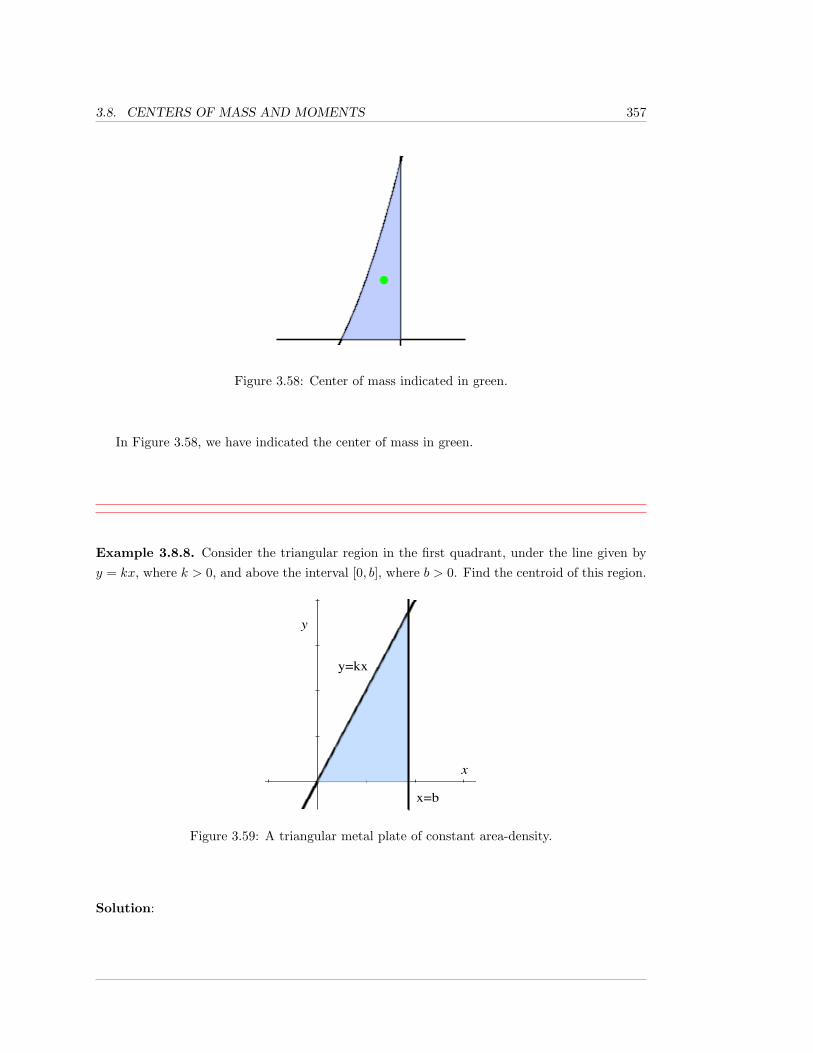
3.8. CENTERS OF MASS AND MOMENTS 357
Figure 3.58: Center of mass indicated in green.
In Figure 3.58, we have indicated the center of mass in green.
Example 3.8.8. Consider the triangular region in the first quadrant, under the line given byy = kx, where k > 0, and above the interval [0, b], where b > 0. Find the centroid of this region.
y=kx
x=b
Figure 3.59: A triangular metal plate of constant area-density.
Solution:
358 CHAPTER 3. APPLICATIONS OF INTEGRATION
As we are finding a centroid, we assume that the area-density δar > 0 is a constant. Theinfinitesimal mass dm of the infinitesimally thin rectangle at x is given by
dm = δar dA = δarkx dx.
The infinitesimal contribution from this rectangle to the x-component of the moment is
x dm = xδarkx dx = δarkx2 dx,
and the infinitesimal contribution from this rectangle to the y-component of the moment is
yx dm =kx+ 0
2δarkx dx =
δark2
2x2 dx.
The mass of the plate is
mass =∫ x=b
x=0
δar dA = δar
∫ x=b
x=0
dA = δar · (area of the plate).
Of course, when the area-density is constant, it’s always true that the mass of the plate is simplyδar times A, the area of the plate. For a more-complicated region, we would have to integrateto find the area and, even here, we could integrate kx to find the area of the triangle, but it’sa triangle; it’s area is 1/2 the base times the height, i.e., A = (1/2)b(kb) = kb2/2. Hence, wehave
M =δarkb
2
2.
The x-component of the moment is
Mx =∫ x=b
x=0
x dm =∫ b
0
δarkx2 dx =
δarkb3
3,
and the y-component of the moment is
My =∫ x=b
x=0
yx dm =∫ b
0
δark2
2x2 dx =
δark2b3
6.
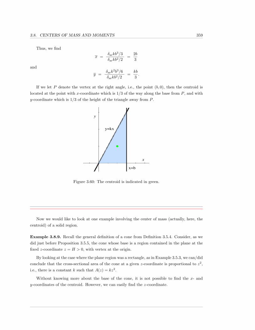
3.8. CENTERS OF MASS AND MOMENTS 359
Thus, we find
x =δarkb
3/3δarkb2/2
=2b3
and
y =δark
2b3/6δarkb2/2
=kb
3.
If we let P denote the vertex at the right angle, i.e., the point (b, 0), then the centroid islocated at the point with x-coordinate which is 1/3 of the way along the base from P , and withy-coordinate which is 1/3 of the height of the triangle away from P .
y=kx
x=b
Figure 3.60: The centroid is indicated in green.
Now we would like to look at one example involving the center of mass (actually, here, thecentroid) of a solid region.
Example 3.8.9. Recall the general definition of a cone from Definition 3.5.4. Consider, as wedid just before Proposition 3.5.5, the cone whose base is a region contained in the plane at thefixed z-coordinate z = H > 0, with vertex at the origin.
By looking at the case where the plane region was a rectangle, as in Example 3.5.3, we can/didconclude that the cross-sectional area of the cone at a given z-coordinate is proportional to z2,i.e., there is a constant k such that A(z) = kz2.
Without knowing more about the base of the cone, it is not possible to find the x- andy-coordinates of the centroid. However, we can easily find the z-coordinate.
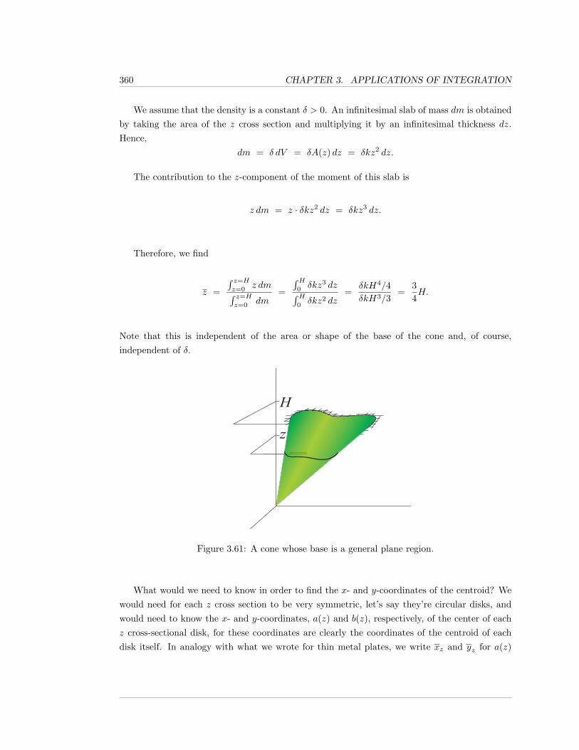
360 CHAPTER 3. APPLICATIONS OF INTEGRATION
We assume that the density is a constant δ > 0. An infinitesimal slab of mass dm is obtainedby taking the area of the z cross section and multiplying it by an infinitesimal thickness dz.Hence,
dm = δ dV = δA(z) dz = δkz2 dz.
The contribution to the z-component of the moment of this slab is
z dm = z · δkz2 dz = δkz3 dz.
Therefore, we find
z =
∫ z=Hz=0
z dm∫ z=Hz=0
dm=
∫H0δkz3 dz∫H
0δkz2 dz
=δkH4/4δkH3/3
=34H.
Note that this is independent of the area or shape of the base of the cone and, of course,independent of δ.
W
lwL
H
H
z
Area B
z
H
z
Figure 3.61: A cone whose base is a general plane region.
What would we need to know in order to find the x- and y-coordinates of the centroid? Wewould need for each z cross section to be very symmetric, let’s say they’re circular disks, andwould need to know the x- and y-coordinates, a(z) and b(z), respectively, of the center of eachz cross-sectional disk, for these coordinates are clearly the coordinates of the centroid of eachdisk itself. In analogy with what we wrote for thin metal plates, we write xz and yz for a(z)
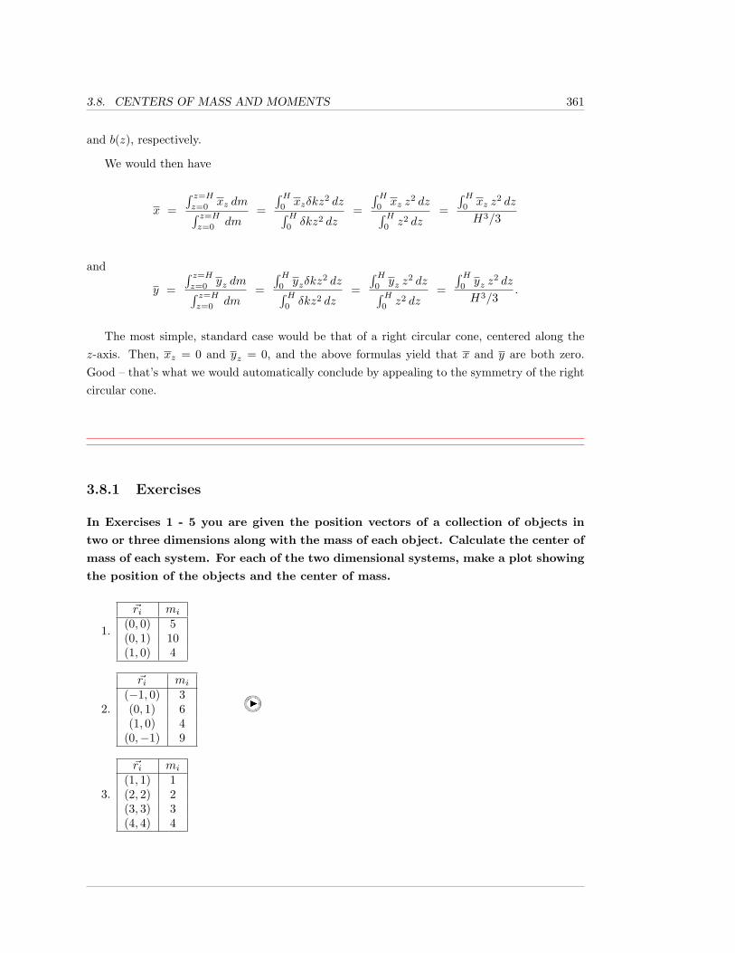
3.8. CENTERS OF MASS AND MOMENTS 361
and b(z), respectively.
We would then have
x =
∫ z=Hz=0
xz dm∫ z=Hz=0
dm=
∫H0xzδkz
2 dz∫H0δkz2 dz
=
∫H0xz z
2 dz∫H0z2 dz
=
∫H0xz z
2 dz
H3/3
and
y =
∫ z=Hz=0
yz dm∫ z=Hz=0
dm=
∫H0yzδkz
2 dz∫H0δkz2 dz
=
∫H0yz z
2 dz∫H0z2 dz
=
∫H0yz z
2 dz
H3/3.
The most simple, standard case would be that of a right circular cone, centered along thez-axis. Then, xz = 0 and yz = 0, and the above formulas yield that x and y are both zero.Good – that’s what we would automatically conclude by appealing to the symmetry of the rightcircular cone.
3.8.1 Exercises
In Exercises 1 - 5 you are given the position vectors of a collection of objects in
two or three dimensions along with the mass of each object. Calculate the center of
mass of each system. For each of the two dimensional systems, make a plot showing
the position of the objects and the center of mass.
1.
~ri mi
(0, 0) 5(0, 1) 10(1, 0) 4
2.
~ri mi
(−1, 0) 3(0, 1) 6(1, 0) 4
(0,−1) 9
3.
~ri mi
(1, 1) 1(2, 2) 2(3, 3) 3(4, 4) 4
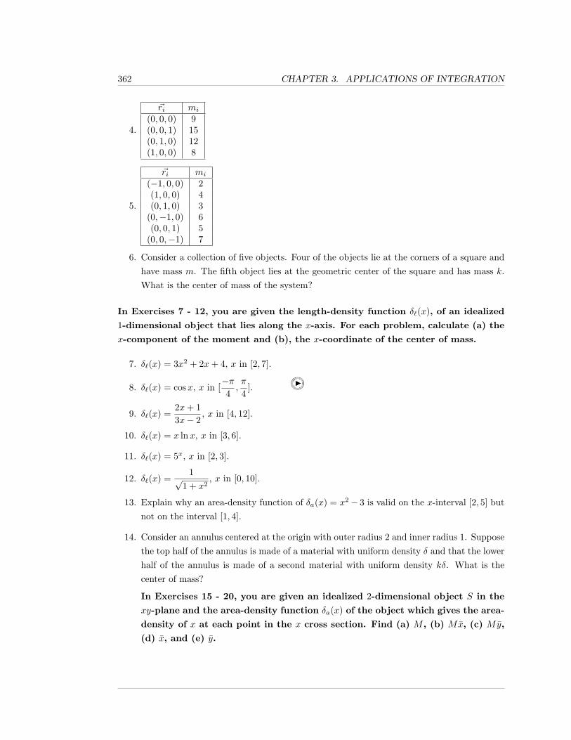
362 CHAPTER 3. APPLICATIONS OF INTEGRATION
4.
~ri mi
(0, 0, 0) 9(0, 0, 1) 15(0, 1, 0) 12(1, 0, 0) 8
5.
~ri mi
(−1, 0, 0) 2(1, 0, 0) 4(0, 1, 0) 3
(0,−1, 0) 6(0, 0, 1) 5
(0, 0,−1) 7
6. Consider a collection of five objects. Four of the objects lie at the corners of a square andhave mass m. The fifth object lies at the geometric center of the square and has mass k.What is the center of mass of the system?
In Exercises 7 - 12, you are given the length-density function δ`(x), of an idealized
1-dimensional object that lies along the x-axis. For each problem, calculate (a) the
x-component of the moment and (b), the x-coordinate of the center of mass.
7. δ`(x) = 3x2 + 2x+ 4, x in [2, 7].
8. δ`(x) = cosx, x in [−π4,π
4].
9. δ`(x) =2x+ 13x− 2
, x in [4, 12].
10. δ`(x) = x lnx, x in [3, 6].
11. δ`(x) = 5x, x in [2, 3].
12. δ`(x) =1√
1 + x2, x in [0, 10].
13. Explain why an area-density function of δa(x) = x2− 3 is valid on the x-interval [2, 5] butnot on the interval [1, 4].
14. Consider an annulus centered at the origin with outer radius 2 and inner radius 1. Supposethe top half of the annulus is made of a material with uniform density δ and that the lowerhalf of the annulus is made of a second material with uniform density kδ. What is thecenter of mass?
In Exercises 15 - 20, you are given an idealized 2-dimensional object S in the
xy-plane and the area-density function δa(x) of the object which gives the area-
density of x at each point in the x cross section. Find (a) M , (b) Mx, (c) My,
(d) x, and (e) y.
3.8. CENTERS OF MASS AND MOMENTS 363
15. S is bounded by the curves f(x) = x and g(x) = x2 between x = 0 and x = 1. δa(x) =2x+ 1.
16. S is a rectangle with vertices (1, 1), (1, 5), (6, 5), and (6, 1), δa(x) = ex.
17. S is the region bounded by the curves f(x) =√
4− x2 and g(x) =√
1− x2, x = −1/2,x = 1/2 and δa(x) = x2 + 1.
18. S is a triangular region with vertices (0, 0), (1, 1) and (−1,−1). δ(a)(x) = 2− x2.
19. S is bounded by the lines f(x) = 3x+ 5, g(x) = x− 3, x = −4 and x = 3, δa(x) = x2 + 5.
20. S is the region below the curve f(x) = cosx and above the line g(x) = 1/2 and x isbetween −π/3 and π/3. δa(x) = |x|+ 1.
21. Find the centroid of the region occupied by the metal plate in Example 3.8.7.
22. What is the centroid of a right circular cone where the base lies in the plane z = 9 andthe vertex is the origin?
23. Consider a cone of uniform density which has a circular disc as its base. The base lies inthe plane z = 1, has center (1, 1, 1) and radius 1. The cone is the union of all line segmentbetween the origin and points on the disc. What is the centroid of the cone?
24. Must there be any mass at the center of mass of a system? If not, give an example.
25. Suppose f(x) is a continuous function on the interval [a, b] and that f(x) > 0. Let S bethe region lying below the graph of f(x), above the x-axis, and between x = a and x = b
and suppose S has constant density δ. Show that the center of mass, or centroid, has
coordinates x =1A
∫ b
a
xf(x) dx and y =1
2A
∫ b
a
f(x)2 dx where A is the area of S.
Use the previous problem to find the centroid of the regions in Exercises 26-31.
Assume the density is constant and that each region lies below the graph of f(x),above the x-axis and between x = a and x = b.
26. f(x) = 2x+ 4, x = 3, x = 7.
27. f(x) = sinx, x = 0, x = π.
28. f(x) = coshx, x = −1, x = 1.
29. f(x) = mx where m > 0, x = 0, x = b.
30. f(x) =√
16− x2, x = −4, x = 4.
31. f(x) = ex, x = 0, x = 1.
364 CHAPTER 3. APPLICATIONS OF INTEGRATION
32. Suppose f and g are two continuous functions on the interval [a, b] and that f > g. LetS be the region lying between the graphs of the two functions and bounded by x = a
and x = b. Assume S has constant density δ and prove the centroid of S has coordinates
x =1A
∫ b
a
x(f(x)− g(x)) dx and y =1
2A
∫ b
a
(f(x)2 − g(x)2
)dx.
Use the previous problem to find the centroid of the regions in Exercises 33 - 38
bounded by the graphs of f(x) and g(x), and by x = a and x = b. Assume in each
case the density is constant.
33. f(x) = 2x+ 9, g(x) = 2x+ 5, x = 4, x = 8.
34. f(x) = 9, g(x) = x2, x = −3, x = 3.
35. f(x) =√
64− x2, g(x) =√
9− x2, x = −3, x = 3.
36. f(x) =√x, g(x) = x, x = 0, x = 1.
37. f(x) = 2ex, g(x) = 2, x = 0, x = 3.
38. f(x) = 5x2 + 3, g(x) = 2x2, x = −2, x = 2.
In Exercises 39 - 44, you are given a dynamic system where a group of particles of
varying masses are moving. The path of the i-th object, which has mass mi, has
position ~pi(t) at time t. Calculate the location of the center of mass as a function
of t.
39. ~p1(t) = (0, 0), ~p2(t) = (t, t), m1 = 8, m2 = 4.
40. ~p1(t) = (t, 0), ~p2(t) = (−t, 0), m1 = 5, m2 = 10.
41. ~p1(t) = (t, 0), ~p2(t) = (−t, 0), ~p3(t) = (0, t), m1 = m2 = 6, m3 = 5.
42. ~p1(t) = (cos 2t, sin 2t), ~p2(t) = (2 cos t, 2 sin t), m1 = 100, m2 = 300. This example modelstwo objects orbiting a central mass-less point. The first ”planet” completes a revolutionin half the time as the outer planet.
43. ~p1(t) = (cos 2t, sin 2t), ~p2(t) = (2 cos t, 2 sin t), ~p3 = (0, 0), m1 = 100, m2 = 300, m3 =1000. This system is similar to the previous one, but now includes a massive ”sun”.
44. ~p1(t) = (−2 + cos t, sin t), ~p2(t) = (2 + cos t, sin t), m1 = 30, m2 = 20.
45. Suppose three particles are initially at rest, and have initial positions ~p1(0) = (−2, 2),~p2(0) = (1,−3), ~p3(0) = (4, 1). At t = 0, a constant external force is applied to eachparticle. The first particle experiences a force of 6 N in the negative x direction, the
3.8. CENTERS OF MASS AND MOMENTS 365
second a force of 14 N in the positive x direction and the third, a force of 16 N in thepositive y direction. The masses of the three particles are 4 kg, 4 kg and 8 kg respectively.
a. Calculate the position function, ~pi(t), for each of the three particles.
b. Calculate the position function of the center of mass at time t. Call this function~c(t).
c. Calculate the magnitude of the acceleration of the center of mass using your answerfrom part (b).
d. What is the total external force acting on the system? Hint: resolve the force into xand y components first.
e. Calculate the magnitude of the acceleration of the center of mass by dividing the totalexternal force acting on the system by the total mass of the system. Your answershould agree with the answer to part (c).
In Exercises 46 - 50 you are given a system similar to that in the previous prob-
lem. Assume each particle starts at rest and that a constant force is applied to
each particle starting at t = 0. For each problem, calculate the magnitude of the
acceleration of the center of mass in two ways: first, by explicitly calculating the
position function of the center of mass, and second, by calculating the total force
acting on the system. The force acting on particle i is given in x and y components.
For example, F1 = (3, 0) indicates a 3 N force in the positive x direction.
46. ~p1(0) = (1, 0), ~p2(0) = (0, 1), F1 = (3, 0), F2 = (0, 3), m1 = 5, m2 = 5.
47. ~p1(0) = (0, 0), ~p2(0) = (2, 3), ~p3(0) = (−1,−3), F1 = (2, 0), F2 = (0,−4), F3 = (−3, 0),
m1 = 3, m2 = 6, m3 = 12.
48. ~p1(0) = (1, 0), ~p2(0) = (0, 1), ~p3(0) = (0, 0), F1 = (2, 0), F2 = (0, 2), F3 = (−2, 0), m1 = 4,m2 = 8, m3 = 12.
49. ~p1(0) = (1, 0), ~p2(0) = (0, 1), ~p3(0) = (−1, 0), ~p4(0) = (0,−1), F1 = (3, 0), F2 = (0, 3),F3 = (−1, 0), F4(0) = (0,−1), m1 = m2 = 1 = m3 = m4 = 5.
50. ~p1(0) = (1, 0, 0), ~p2(0) = (0, 1, 0), ~p3(0) = (0, 0, 1), ~p4(0) = (0, 0, 0), F1 = (2, 0, 0), F2 =(0, 3, 0), F3 = (0, 0, 4), F4(0) = (0,−3, 0), m1 = m2 = 6, m3 = m4 = 12.
366 CHAPTER 3. APPLICATIONS OF INTEGRATION
3.9 Work and Energy
The technical notion of work does not coincide precisely with what is frequently referred to aswork in day-to-day speech. Work is defined to be force applied over a displacement. We shallclarify this below, but, for now, we want to emphasize that, if an object does not move, thenno work is done on the object. This conflicts with what most people would refer to as the workrequired to hold some heavy weight motionless in their hands. We have a tendency to think ofwork as corresponding to applying force over a period of time, not over a displacement; whenyou’re in a physics or mathematics class, you need to stop thinking this way.
Work is, in a technical sense, equivalent to energy, though we usually use the terms slightlydifferently when speaking and writing. We typically say things like “it takes energy to producework”, but it’s also true that the work done on a object can get “converted” into kinetic energy,potential energy, heat, etc. All of this falls under the heading of the principle of Conservation ofEnergy, which states that energy cannot be created or destroyed, merely converted from one formto another. Since the work of Einstein showed that mass can be converted into energy, accordingto the famous equation E = mc2, which was first put into practice with the development of theatomic bomb, the principles of Conservation of Energy and Conservation of Mass are frequentlynow combined, and referred to as Conservation of Mass-Energy.
Assume that we have an object whose motion is constrained to a straight line, which we taketo be the x-axis. We suppose that we have a constant force F which acts parallel to the x-axis,with the sign of F indicating the direction of the force. If the object begins at x-coordinate x0
and ends up at x-coordinate x1, then the displacement of the object is ∆x = x1 − x0.
Definition 3.9.1. The work done by the constant force F on the object, in displacing theobject ∆x, is F∆x.
In the metric system, the standard unit of work/energy is 1 joule, which is equal to 1Newton-meter. In the English system, you simply use the foot-pound.
Remark 3.9.2. Note that work can be positive or negative. If the force is in the direction of thedisplacement, i.e., if the force and displacement are both positive, or the force and displacementare both negative, then the work is positive. However, if the force and displacement are in
3.9. WORK AND ENERGY 367
opposite directions, then the work is negative. For example, suppose that we exert a forceupward, raising an object against the force of gravity. Then, we do (or, our force does) positivework on the object. However, gravity does negative work on the object during that displacement.
Instead of saying that a particular force does work, it is common to say that whatever isproducing the force does the work. For instance, if Sally pushes an object along the ground,then we would usually say that Sally does work on the object, rather than refer to the force thatSally exerts.
So, what do we do when the force is not constant? We do what we always do: chop thingsup into small pieces, over which we can assume that the force is approximately constant. Then,we take Riemann sums, and limits, to arrive at the definite integral. Infinitesimally, we writesimply that the infinitesimal work dW done by F in displacing an object by the infinitesimalamount dx is dW = F dx, and so:
Proposition 3.9.3. If a continuous force F = F (x) (parallel to the displacement) acts onan object, as the object is displaced from x0 to x1, then the work W done by F on the objectis given by
W =∫ x1
x0
F dx.
Remark 3.9.4. In some of our later problems, in which we look at lifting liquid out of a tank,it will be more natural to consider the amount of displacement q as a function of the force,i.e., we will use that, essentially, q is a function of F . This means that, instead of using thatdW = F dx, we will use that dW = q dF .
Example 3.9.5. Suppose, when an object is located at position x meters, that the objectexperiences a force of F = −k/x2 Newtons, where k is a positive constant. Find, in terms of k,how much work the force does on the object, as the object moves from x = 2 to x = 1 meter.
Solution: We simply calculate
W =∫ 1
2
F dx =∫ 1
2
− k
x2dx = −k
∫ 1
2
x−2 dx = −k · x−1
−1
∣∣∣12
=
368 CHAPTER 3. APPLICATIONS OF INTEGRATION
k
(1− 1
2
)=
k
2joules.
Before we look at more examples, it will be useful to first discuss the work/energy equivalenceand, in particular, discuss the relationship between work, kinetic energy, and (gravitational)potential energy.
Definition 3.9.6. The kinetic energy of an object of mass m, moving with speed v, is
EK =12mv2.
Note that it is classical to use v in the formula for kinetic energy, even though the v is speed,not velocity. For motion in a straight line, where the direction of the velocity is given by a plusor minus sign, the distinction between speed and velocity in the calculation of the kinetic energyis irrelevant, for v is squared. However, for the more general situation of arbitrary motion isspace, it is important that you use speed in calculating the kinetic energy.
The relationship between work and kinetic energy is given by:
Theorem 3.9.7. Suppose that F is the sum of all forces acting (along the x-axis) on anobject of constant mass m, at all times between t0 and t1, where t0 < t1. Suppose thatthe position x = x(t) of the object is continuously differentiable, that the velocity v is acontinuously differentiable function of x.
Let x0 and x1 denote the positions of the object, at times t0 and t1, respectively, and letv0 and v1 denote the velocities of the object, at positions x0 and x1, respectively.
Then, F is a continuous function of x, and the work done by F in displacing the object fromx0 to x1 is given by
W =∫ x1
x0
F dx =12mv2
1 −12mv2
0 ,
i.e., the work done by the net force is equal to the change in kinetic energy.
Proof. Let v = dx/dt denote the velocity. By Newton’s 2nd Law of Motion,
F = ma = mdv
dt= m
dv
dx· dxdt
= mdv
dxv,
3.9. WORK AND ENERGY 369
where the third equality follows from the Chain Rule.
Thus,
W =∫ x1
x0
F dx =∫ x1
x0
mvdv
dxdx =
∫ v1
v0
mv dv =12mv2
1 −12mv2
0 .
Example 3.9.8. Suppose that x(t) = 4− t2 is the position function, in meters, of a 10 kilogramobject, which is moving along the x-axis between times t = 0 and t = 3 seconds. Calculate thework done in displacing the object from x(0) = 4 meters to x(3) = −5 meters.
Solution:
By Theorem 3.9.7, all that matters is the change in kinetic energy, so we need the velocitiesat times t = 0 and t = 3. We find
v(t) = x′(t) = −2t m/s.
Thus the work done is
12
(10)(v2(3)− v2(0)) = 5((−6)2 − 02
)= 180 joules.
Remark 3.9.9. A special application of Theorem 3.9.7 comes up fairly often.
Suppose that some force Fext, which we’re thinking of as external, acts on an object withconstant mass, and that the only other force is Fyou, exerted by you (or anything/anyone else).Then, the total force F acting on the object is F = Fext + Fyou. Suppose that the initial speedof the object is equal to the final speed of the object; frequently, we consider the case where theobject starts at rest, i.e., with zero velocity, and ends up at rest.
370 CHAPTER 3. APPLICATIONS OF INTEGRATION
Then, Theorem 3.9.7 tells us that
∫ x1
x0
F dx =∫ x1
x0
(Fext + Fyou) dx = 0,
i.e., ∫ x1
x0
Fyou dx =∫ x1
x0
−Fext dx. (3.3)
In words, if an object starts and ends with the same kinetic energy, then the work that youdo on the object is the negative of the work done by the external force; this is frequently referredto as the work done against Fext.
Note that Formula 3.3 is correct even though, usually, it would not be the case, at everytime or position, that Fyou is equal to −Fext. For instance, if you begin with an object at rest,and apply a force to lift it, acting against the force of gravity, −mg, and end with the objecthigher, at rest, then the force that you exert cannot always be equal to mg; for you must applya force greater than mg to make the mass accelerate, i.e., to make it start moving upward, andyou must apply a force less than mg later in order for the mass to decelerate back down to zerovelocity.
It is crucial in Theorem 3.9.7 and in Formula 3.3 that the mass of the object is constant.In our derivations, we used Newton’s 2nd Law of Motion that the net force, F , acting onan object is equal to the mass times the acceleration, ma. This may not be correct if themass is changing. See Remark 3.9.17. Even if F = ma, we used that m was constant whenwe found that
∫mv dv = mv2/2 + C.
Definition 3.9.10. The (gravitational) potential energy of an object of mass m, at heighth above the surface of the Earth, is
EP = mgh,
where g is the acceleration due to gravity on Earth.
We have assumed in the above formula that the heights involved are small enough that theforce of gravity on the object does not vary significantly. We have also taken zero potential
3.9. WORK AND ENERGY 371
energy to correspond to zero height; however, in fact, it is really only the change in potentialenergy that occurs in calculations, and so, if it’s more convenient to take the zero potentialenergy location elsewhere, you can do so.
Remark 3.9.9 applies to the case of (gravitational) potential energy.
Theorem 3.9.11. Suppose that a force Fyou is used to raise an object of mass m from restat height h = h0 (above the surface of the Earth) to rest at height h = h1, and that the onlyother force acting on the object is the force of gravity. Make the same assumptions on thecontinuity and differentiability of the velocity and position functions as in Theorem 3.9.7(using, here, h in place of x).
Then, the work done by the force Fyou is
W =∫ h1
h0
Fyou dh = mgh1 −mgh0,
i.e., the work done by the force Fyou is equal to the change in potential energy.
Proof. There are two forces acting on the object: Fyou and the force of gravity, −mg. ByRemark 3.9.9, we find
∫ h1
h0
Fyou dh =∫ h1
h0
−(−mg) dh = mg(h1 − h0).
Remark 3.9.12. In what sense is potential energy actually energy? The potential energy ofan object is actually the potential energy of the object relative to an ambient (surrounding orexternal) force. What we mean is that, in the presence of the gravitational field of the Earth, ifyou release an object of mass m from rest, at a height h above the ground, the object will fall,increasing its speed. In fact, ignoring air resistance, Theorem 3.9.7 tells us that the work doneby the force of gravity will convert the object’s potential energy into kinetic energy; you cancalculate the speed v at which the object will strike the ground simply by solving for v in the
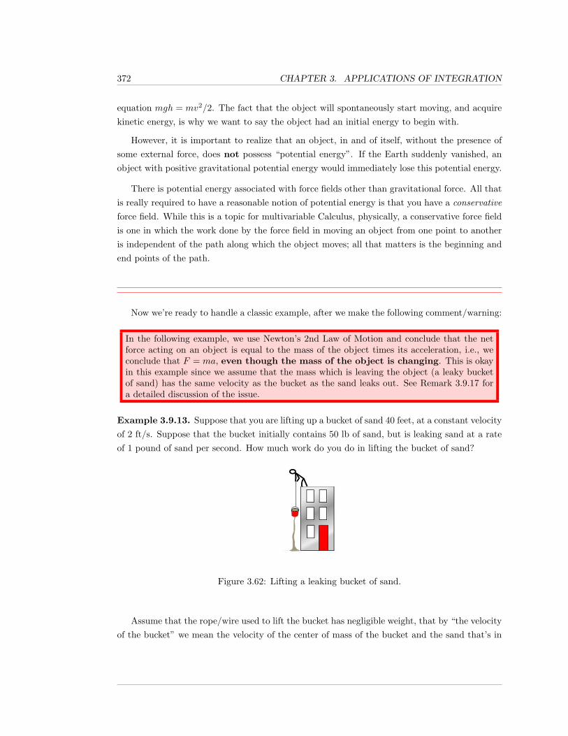
372 CHAPTER 3. APPLICATIONS OF INTEGRATION
equation mgh = mv2/2. The fact that the object will spontaneously start moving, and acquirekinetic energy, is why we want to say the object had an initial energy to begin with.
However, it is important to realize that an object, in and of itself, without the presence ofsome external force, does not possess “potential energy”. If the Earth suddenly vanished, anobject with positive gravitational potential energy would immediately lose this potential energy.
There is potential energy associated with force fields other than gravitational force. All thatis really required to have a reasonable notion of potential energy is that you have a conservativeforce field. While this is a topic for multivariable Calculus, physically, a conservative force fieldis one in which the work done by the force field in moving an object from one point to anotheris independent of the path along which the object moves; all that matters is the beginning andend points of the path.
Now we’re ready to handle a classic example, after we make the following comment/warning:
In the following example, we use Newton’s 2nd Law of Motion and conclude that the netforce acting on an object is equal to the mass of the object times its acceleration, i.e., weconclude that F = ma, even though the mass of the object is changing. This is okayin this example since we assume that the mass which is leaving the object (a leaky bucketof sand) has the same velocity as the bucket as the sand leaks out. See Remark 3.9.17 fora detailed discussion of the issue.
Example 3.9.13. Suppose that you are lifting up a bucket of sand 40 feet, at a constant velocityof 2 ft/s. Suppose that the bucket initially contains 50 lb of sand, but is leaking sand at a rateof 1 pound of sand per second. How much work do you do in lifting the bucket of sand?
Figure 3.62: Lifting a leaking bucket of sand.
Assume that the rope/wire used to lift the bucket has negligible weight, that by “the velocityof the bucket” we mean the velocity of the center of mass of the bucket and the sand that’s in
3.9. WORK AND ENERGY 373
it, and that the instantaneous velocity of the sand as it leaves the bucket is equal to the velocityof the bucket, i.e., assume that the escaping sand leaves the bucket with velocity 2 ft/s (andthen starts decelerating once gravity is the only force acting on it).
Note that gravity acts downward, while the displacement is upward. Thus, the work done bygravity will be negative, while the work that you do will be positive. We take the accelerationof gravity to be g = 32 ft/s2.
Set up a y-axis vertically, with 0 at the initial position of the bucket, and the positivedirection being upward. Let t be the amount of time elapsed, in seconds, from the time at whichyou start raising the bucket.
The force of gravity Fgrav on the bucket is its weight, with a minus sign, to indicate thatgravity acts downward. As the bucket initially weighs 50 lb, and loses 1 pound per second, wehave
Fgrav = −(50− t) lb.
But we need Fgrav as a function of y, so that we can calculate the work done by gravity Wgrav =∫ 40
0Fgrav dy.
Since the bucket is moving with a constant velocity of 2 ft/s, the position of the bucket attime t seconds is y = 2t feet. Hence, t = y/2, and so
Fgrav = −(
50− y
2
)lb.
As we mentioned before starting this problem, since the sand is leaving the bucket at thesame velocity as the bucket, the total/net force F = Fyou + Fgrav acting on the bucket is ma,where m is the mass of the bucket of sand and a is its acceleration. But, the bucket of sand ismoving with constant velocity; so a = 0, and we conclude that
F = Fyou + Fgrav = 0,
i.e., that Fyou = −Fgrav =(50− y
2
)ft-lb.
Now, we calculate easily
Wyou =∫ 40
0
Fyou dy =∫ 40
0
(50− y
2
)dy =
(50y − y2
4
)∣∣∣∣40
0
=
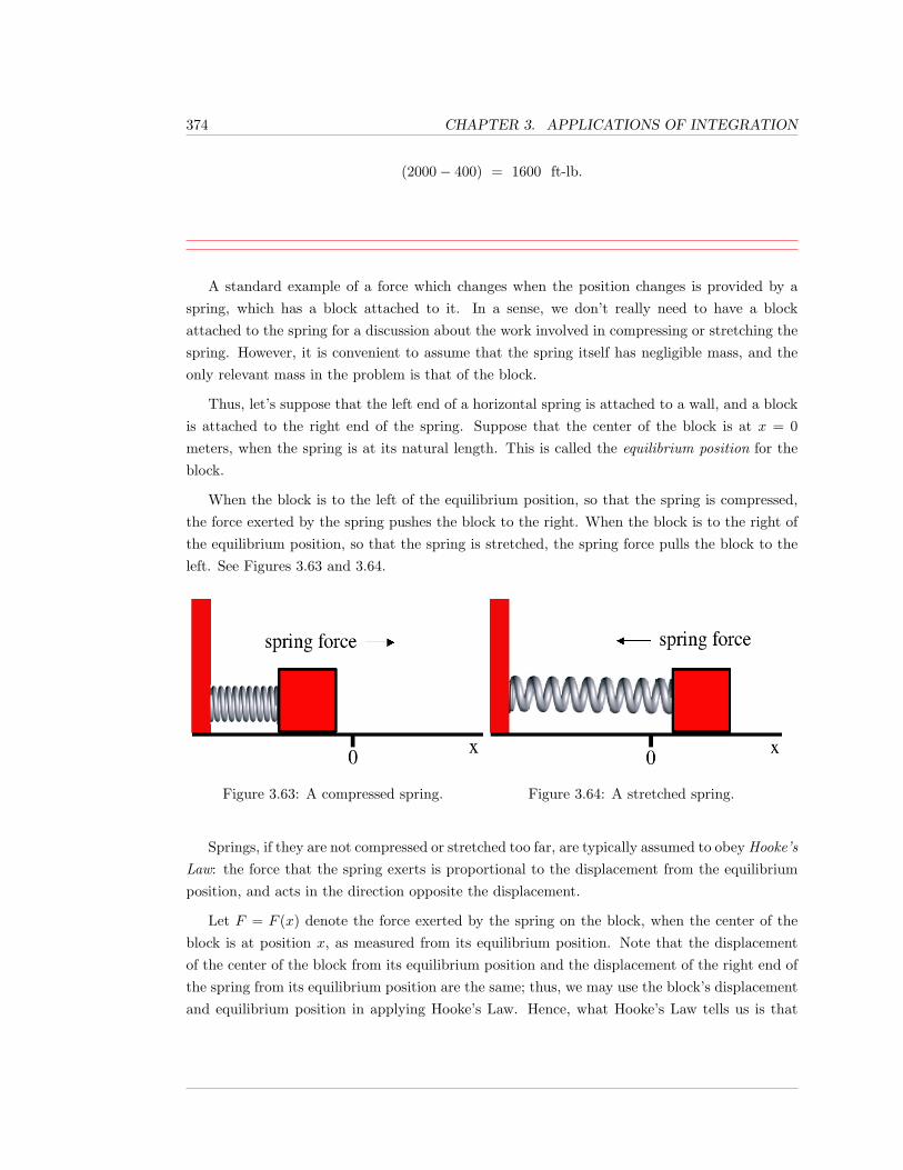
374 CHAPTER 3. APPLICATIONS OF INTEGRATION
(2000− 400) = 1600 ft-lb.
A standard example of a force which changes when the position changes is provided by aspring, which has a block attached to it. In a sense, we don’t really need to have a blockattached to the spring for a discussion about the work involved in compressing or stretching thespring. However, it is convenient to assume that the spring itself has negligible mass, and theonly relevant mass in the problem is that of the block.
Thus, let’s suppose that the left end of a horizontal spring is attached to a wall, and a blockis attached to the right end of the spring. Suppose that the center of the block is at x = 0meters, when the spring is at its natural length. This is called the equilibrium position for theblock.
When the block is to the left of the equilibrium position, so that the spring is compressed,the force exerted by the spring pushes the block to the right. When the block is to the right ofthe equilibrium position, so that the spring is stretched, the spring force pulls the block to theleft. See Figures 3.63 and 3.64.
Figure 3.63: A compressed spring. Figure 3.64: A stretched spring.
Springs, if they are not compressed or stretched too far, are typically assumed to obey Hooke’sLaw: the force that the spring exerts is proportional to the displacement from the equilibriumposition, and acts in the direction opposite the displacement.
Let F = F (x) denote the force exerted by the spring on the block, when the center of theblock is at position x, as measured from its equilibrium position. Note that the displacementof the center of the block from its equilibrium position and the displacement of the right end ofthe spring from its equilibrium position are the same; thus, we may use the block’s displacementand equilibrium position in applying Hooke’s Law. Hence, what Hooke’s Law tells us is that
3.9. WORK AND ENERGY 375
there exists a positive constant k such that
F = −kx.
The constant k depends on the spring in question, and is called the spring constant.
Example 3.9.14. Suppose that a spring has spring constant k = 50 N/m. How much workdoes it take to compress the spring 1 meter from the equilibrium position?
Solution:
While it is not stated explicitly in the problem, it is implicit that the spring/mass startsat rest and ends at rest. In addition, unlike the leaky bucket problem in Example 3.9.13, themass is not changing. Hence, we may apply Formula 3.3 to conclude that the work done by thecompressing force is negative the work done by the spring, i.e.,
∫ −1
0
Fcomp dx =∫ −1
0
−Fspring dx =∫ −1
0
−(−kx) dx =kx2
2
∣∣∣∣−1
0
= 25 joules.
Now we come to two examples where, instead of using that an infinitesimal amount of workdW is F dx, we use that dW = q dF , where dF is an infinitesimal amount of force and q is thedisplacement of the mass on which dF acts.
Example 3.9.15. Suppose that we have a tank, which is a right circular cylinder of radius 8feet and height 30 feet. The tank contains water up to a height of 10 feet (and the rest of thetank is empty). Assume that the weight-density of water (weight per volume, a.k.a., the specificweight) is δw = 62.4 lb/ft3.
We want to find the amount of work required to pump all of the water to the top of the tank.We are not discussing any extra work involved in then moving the water off to a pipe at somelocation at the top of the tank; in particular, we mean the work involved in moving the waterto the top of the tank at rest. As the water is not initially moving, and we are calculating thework involved in leaving the water at the top of the tank at rest, the work involved in pumpingthe water is negative the work that gravity does on the water as we move the water to the top,i.e., the work done against gravity.
376 CHAPTER 3. APPLICATIONS OF INTEGRATION
Okay. So how do we find the work done against gravity? Set up a z-axis, with z = 0 atthe bottom of the tank, and with the positive direction being up. For each z-coordinate wherewe have water, that is, for z between 0 and 10, we calculate the work involved in lifting theinfinitesimally thickened z cross section of water. We then add up, i.e., take the integral of, allof these infinitesimal pieces of work as z goes from 0 to 10.
Consider the infinitesimally thickened z cross section of water. As in Section 3.5, the in-finitesimal volume of this piece is dV = A(z) dz, where A(z) is the cross-sectional area. In ourcurrent setting, A(z) is constant; it’s the area inside a circle of radius 8 feet. Thus, A(z) = 64πft2, and dV = 64π dz. The (negation of the) infinitesimal force that gravity exerts of this chunkof volume is
dF = δw dV = (62.4)(64π) dz lb.
How much do we have to displace the slab of volume at coordinate z to get it to the top of thetank? As the tank is 30 feet high, the needed displacement is 30−z feet. Thus, the infinitesimalwork done against gravity in order to lift the infinitesimally thick piece of volume at a givenz-coordinate between 0 and 10 is
dW = (30− z) dF = (30− z)(62.4)(64π) dz ft-lb.
Therefore, the total work required to move all of the water to the top of the tank is
W =∫ z=10
z=0
dW =∫ 10
0
(30− z)(62.4)(64π) dz = (62.4)(64π)(
30z − z2
2
)∣∣∣∣10
0
=
(62.4)(64π) (300− 50) ≈ 3, 136, 566.1 ft-lb.
Note that the limits of integration refer to the z-coordinates at which there is water whichneeds to be lifted. It is a common mistake to let z go from 0 to the height of the tank. Keepin mind what the integral is doing: it’s adding up all of the infinitesimal pieces of work fromeach of the z cross sections at which there’s water that’s being lifted.
We could have obtained this same answer in a different way. In Exercise 32, we ask you toshow something that you may have guessed: that you can calculate the work in this problem(or any problem like it) by taking the total weight of the water and then multiplying by the“right” displacement. What is this right displacement? The distance between z-coordinate ofthe center of mass of the water and the top of the tank.
In more-complicated problems, calculating the work by finding the total weight and z-coordinate of the center of mass would not be significantly easier than calculating a corre-
3.9. WORK AND ENERGY 377
sponding work integral. However, in our current problem, the calculation via the center of massis trivial. By symmetry, the z-coordinate of the center of mass is z = 5 feet. The total weightof the water is δw = 62.4 lb/ft3 times the volume of a right circular cylinder of radius 8 feet andheight 10 feet. Therefore, we quickly find that work required to move all of the water to the topof the tank is
(62.4)(64π)(10)(30− 5) ft-lb,
which, of course, agrees with what we calculated above.
In this example, we change the tank from the previous problem; instead of using a rightcircular cylinder, we use an upside-down cone.
Example 3.9.16. Suppose that we have a tank, which is a right circular cone, which is (mys-teriously) balancing on its point. Suppose that the top radius of the cone is 8 feet and height is30 feet. The tank contains water up to a height of 10 feet (and the rest of the tank is empty).Assume that the weight-density of water (weight per volume) is δw = 62.4 lb/ft3. We once againwant to find the amount of work required to pump all of the water to the top of the tank.
What changes from our previous example? In a sense, very little. The only thing thatchanges is our formula for the cross-sectional area of the tank at a given z value between 0 and10 feet. Our z cross sections are still disks, but the radius of the disks gets smaller as we getcloser to the bottom of the tank.
By using similar triangles, we quickly conclude that the radius r of the cross section at zsatisfies
z
30=
r
8, and so r =
4z15.
Therefore, the cross-sectional area is given by
A(z) = π
(4z15
)2
=16πz2
225ft2.
Hence, instead of calculating
W =∫ z=10
z=0
dW =∫ 10
0
(30− z)(62.4)(64π) dz,
378 CHAPTER 3. APPLICATIONS OF INTEGRATION
which is what we did in Example 3.9.15, we need to calculate
W =∫ z=10
z=0
dW =∫ 10
0
(30− z)(62.4)(
16πz2
225
)dz.
We find
W =(62.4)(16π)
225
∫ 10
0
(30z2 − z3) dz =(62.4)(16π)
225
(10z3 − z4
4
)∣∣∣∣10
0
=
(62.4)(16π)225
(10, 000− 2500) ≈ 104, 552.2 ft-lb.
We end this section with a serious discussion of Newton’s 2nd Law of Motion for objectswith changing mass. We should explicitly mention that this is part of Newtonian Mechanics,and does not include a discussion that takes Einstein’s theories of relativity into account; thismeans that we are dealing with velocities which are small compared to the velocity of light, sothat the relativistic effects are insignificant.
Remark 3.9.17. When an object changes mass, it either gains or loses mass, and the appro-priate form of Newton’s 2nd Law depends on the relative velocity of the center of mass of theobject and the mass which is gained or lost. Understand that part of the issue with changingmass is that what we are calling “the object” changes; we suddenly start calling the old object,together with the new particles that joined it, the “new object”, or we stop referring to particlesthat used to be part of the object as part of the “new object”.
Let m denote the mass of the object at time t, and let F denote the net force acting on theobject. Then, dm/dt will be positive if the object is gaining mass and negative if the object islosing mass. Let vrel denote the velocity, relative to the velocity of the center of mass of theobject, of the gained or lost mass instantaneously as it joins or departs the object; that is, vrel
is the velocity of the center of mass of the gained or lost mass according to someone is movingalong with the center of mass of the object, and who considers their own velocity to be zero.This means that if an outside observer says that the velocity of the center of mass of the objectis v and the velocity of the center of mass of the gained or lost mass is vgl, then
vrel = vgl − v.
3.9. WORK AND ENERGY 379
Then, the correct form of Newton’s 2nd Law is
F = mdv
dt− vrel
dm
dt= ma + (v − vgl)
dm
dt. (3.4)
Therefore, if the center of mass of the mass that is gained or lost is moving at the same velocityas the center of mass of the object, such as in the leaky bucket problem in Example 3.9.13, thenv − vgl = 0 and Formula 3.4 collapses to the familiar
F = ma.
On the other hand, if vgl = 0, so that vrel = −v, then Formula 3.4 becomes
F = mdv
dt+ v
dm
dt=
d(mv)dt
,
i.e., the net force equals the rate of change of the momentum, with respect to time. Thissituation is a reasonable approximation of what happens as hail gains mass as it falls throughthe atmosphere and smashes into essentially motionless water molecules, which become part ofthe hail. This case may also apply to a rocket, if the rocket is expelling burned fuel at velocity0, i.e., at velocity −v, relative to the rocket.
We should remark that you need to be careful with Conservation of Energy calculations whenobjects collide or separate. When objects collide, momentum is conserved, but kinetic energyneed not be conserved; some of the kinetic energy present before the collision may be “used up”in deforming the objects which are colliding. These deformations involve the objects heatingup, so that some of the kinetic energy is converted into heat. Such a collision, in which kineticenergy is not conserved, is called an inelastic collision. Thus, in an inelastic collision, the totalkinetic energy drops. A collision in which the objects actually merge to form one object, suchas when motionless water molecules attach to hail, is referred to as totally inelastic.
When objects separate, there is the analogous concept of a totally inelastic separation. In atotally inelastic separation, the kinetic energy goes up. This implies that extra energy had tocome from somewhere, such as a chemical reaction which releases heat. A typical example ofthis is when a rocket expels burned/burning fuel.
380 CHAPTER 3. APPLICATIONS OF INTEGRATION
3.9.1 Exercises
In Exercises 1 through 5, calculate the work done in moving a particle subject to
the force F (x) as it moves between the endpoints of the interval. Assume that x is
position of the particle along the x-axis, measured in meters, and F is measured in
Newtons.
1. F (x) = 3x2 − 2x+ 1, −3 ≤ x ≤ 6.
2. F (x) = 4 sin(2x) + lnx, 1 ≤ x ≤ π.
3. F (x) =3x2
, 5 ≤ x ≤ 9.
4. F (x) =x2 + x+ 1x+ 1
, 0 ≤ x ≤ 4.
5. F (x) = 5e−4x, 1 ≤ x ≤ 3.
6. You exert a force Fyou on an object. The only other force acting on the object is an externalforce, Fext. The object is moving along the x-axis. If the initial and final positions of theobject are the same, is it true that the total work experienced by the object is zero?Explain your answer.
7. You exert a force Fyou on an object. The only other force acting on the object is anexternal force, Fext. The object is moving along the x-axis. If the initial and final speedsof the object are the same, is it true that the total work experienced by the object is zero?Explain your answer.
In Exercises 8 through 12, you are given the position function x(t) of an object with
constant mass m kilograms moving along the x-axis between times t0 and t1. Cal-
culate the work done in displacing the object from x(t0) to x(t1). The displacement
is measured in meters and time is measured in seconds.
8. x(t) = cos t, t0 = 0, t1 = π/2.
9. x(t) = cos t, t0 = 0, t1 = π.
10. x(t) = −4.9t2 + 2t+ 100, t0 = 0, t1 = 3.
11. x(t) = 3 ln(t+ 1), t0 = 0, t1 = 9.
12. x(t) = cosh t, t = 0, t = 4.
3.9. WORK AND ENERGY 381
In Exercises 13 through 17, an object experiences a force depending on its position
x, and a constant k. The total work, W , done by the force on the object as it moves
along the x-axis from positions x0 to x1 is also given. Solve for k. W is measured in
joules, F is measured in Newtons, and displacement is measured in meters.
13. F = −k/x2, x0 = 2, x1 = 1, W = 112.
14. F = x+ k, x0 = 3, x1 = 12, W = 96.
15. F = −k/x, x0 = 4, x1 = 8, W = 80.
16. F = kex, x0 = 0, x1 = 3, W = 72.
17. F = kx2, x0 = 4, x1 = 5, W = 3.
In Exercises 18 through 22, you are given the mass and velocity, v(x), of an object
moving along the x-axis as a function of its position. Calculate the total work done
as the object moves from x0 to x1. Mass is measured in kilograms, velocity in meters
per second, and displacement in meters.
18. v(x) = 3x2 + 2, m = 12, x0 = 2, x1 = 5.
19. v(x) = 9, m = 15, x0 = 2, x1 = 29.
20. v(x) = sinπx, m = 20, x0 = 0, x1 = 1.
21. v(x) = |9x− 2|, m = 9, x0 = 1, x1 = 3.
22. v(x) = e−x2, m = 11, x0 = 5, x1 = 5.
23. A worker is cleaning windows on a tall building. The combined mass of the worker andthe lift used to transport him is 150 kg. If the distance between each floor is 3 meters,how much work is required to elevate the worker and the lift from the 12th to the 22ndfloor?
24. A ball is dropped from a height of 50 meters. What is the speed of the ball when it hitsthe ground? Solve by equating formulas for potential and kinetic energy.
25. Redo Example 3.9.13 under the following assumptions: the bucket of sand is lifted atconstant velocity 4 ft/s. The bucket initially contains 80 lb of sand and the sand is leakingat a rate of 0.5 lb per second. How much work is done lifting the sand 60 feet?
382 CHAPTER 3. APPLICATIONS OF INTEGRATION
26. Consider a bucket-lifting problem where all the initial data is the same, as in Exam-ple 3.9.13, with the following exceptions: The bucket is to be lifted to a height of 120 feetinstead of 40 feet. The bucket leaks sand until only 1 lb of residual sand remains. Howmuch work is done in lifting the bucket to 120 feet?
27. Generalize Example 3.9.13: Suppose that you are a lifting a bucket of sand h feet at aconstant velocity v ft / s. The bucket initially contains P0 lb of sand, but is leaking sand
at a rate of r pounds of sand per second. Assume P0 >rh
v. How much work is done in
lifting the bucket?
In Exercises 28 through 30, calculate the work required to compress the spring with
the given constant by d meters from the equilibrium position. Use Hooke’s Law.
28. k = 10 N/m, d = 2 meters.
29. k = 12 N/m, d = 3 meters.
30. k = 6 N/m, d = 5 meters.
31. Generalize Theorem 3.9.11 by removing the assumptions that the initial and final velocitiesof the object are zero, and calculating
∫ h1
h0Fyou dh in terms of changes in the potential
energy and the kinetic energy of the object.
32. Suppose that a tank has height H and has z cross-sectional area given by the continuousfunction A(z), where z = 0 corresponds to the bottom of the tank, and up is the positive zdirection. Suppose also that the tank contains a liquid, which fills the portion of the tankbetween z = 0 and z = b, where 0 ≤ b ≤ H, and that, at each fixed z-coordinate between0 and b, every point in the z cross section has the same weight-density δw(z). Finally,suppose that δw(z) is continuous.
Show that the work required to pump all of the liquid to the top of the tank is equalto the total weight of the liquid times the distance between the top of the tank and thez-coordinate of the center of mass of the liquid.
We now consider a particle which is subjected to a force as the particle travels along
a path in three dimensions. We use the vector material in Appendix A.
Let ~α(t) = (x(t), y(t), z(t)) be a parameterization of the path where a < t < b.
Suppose that ~F : R3 → R3 is a vector force field. Then, we define the work done by
the force to the particle along the path using integration and the dot product:
Work =∫ b
a
~F (~α(t)) · ~α′(t) dt.
3.9. WORK AND ENERGY 383
Here, we are assuming that ~F is continuous and ~α is differentiable. Note that even
though the particle is traveling in three dimensions, the calculation of work involves
a one-dimensional integral.
33. Suppose ~F (x, y, z) = (2x, xyz, 5 − z), is a vector force field acting on a particle whoseposition is given by ~α(t) = (t2, t, 5), 1 < t < 2.
a. Show that ~F (~α(t)) = (2t2, 5t3, 0).
b. Show that ~F (~α(t)) · ~α ′(t) = 9t3.
c. Calculate the work done by ~F on the particle on the path α(t) by calculating∫ 2
1
9t3 dt.
In Exercises 34 through 38, calculate the work done on a particle by the force field~F as the particle moves along the parameterized path. ~F is in Newtons, distances
are in meters, and time is in seconds.
34. ~F (x, y, z) = (y, x, z2), ~α(t) = (cos t, sin t, t), 0 < t < 2π.
35. ~F (x, y, z) = (yz, xz, xy), ~α(t) = (2t, t,−3t), −1 < t < 1.
36. ~F (x, y, z) = (3x2 − 2x+ 1, 0, 0), ~α(t) = (t, 0, 0), −3 < t < 6. Note that this is just anotherway of presenting Exercise 1 of this section.
37. ~F (x, y, z) = (sinhx, y, z), ~α(t) = (0, 5 sin t, 5 cos t), 0 < t < 2π.
38. ~F (x, y) =(−y
x2 + y2,
x
x2 + y2
), ~α(t) = (cos t, sin t), 0 < t < 2π. In this case, the particle’s
path and the force field are both two dimensional. We can fit this exercise into ourdefinitions above by declaring the third components of both the particle’s path and theforce field to be constantly zero.
In Exercises 39 through 42, it will be helpful to recall Example 3.9.15 and Exam-
ple 3.9.16. In particular, you should use that the weight-density of water is δw = 62.4lb/ft3.
39. A rectangular tank has length 20 feet, width 8 feet, and height 30 feet. The tank containswater up to a height of 10 feet (and the rest of the tank is empty). Find the amount ofwork required to pump all of the water to the top of the tank.
40. Suppose that we have a tank, which is a right circular cylinder of radius 8 feet and height30 feet, and the tank is initially full. Find the amount of work required to pump all of thewater to the top of the tank.
384 CHAPTER 3. APPLICATIONS OF INTEGRATION
41. Suppose that we have a tank, which is a right circular cone, which is balancing on its point.Suppose that the tank is full, and that the top radius of the cone is 8 feet and height is 30feet. Find the amount of work required to pump all of the water to the top of the tank.
42. Suppose that we have a tank, which is a right circular cone, which has its circular base atthe bottom, and its vertex at the top. Suppose that the radius of the base is 8 feet andheight is 30 feet. The tank contains water up to a height of 10 feet (and the rest of thetank is empty). Find the amount of work required to pump all of the water to the top ofthe tank.
3.10. HYDROSTATIC PRESSURE 385
3.10 Hydrostatic Pressure
The term “hydrostatic pressure” refers to pressure that acts on a surface which is submergedin motionless water (“static” for motionless, “hydro” for water), and while we shall, in fact,discuss mainly the case of water on Earth, our discussion applies to essentially any body ofliquid anywhere.
When an object is partially, or totally, submerged in a liquid, such as water, the surfaces ofthe object which are exposed to the liquid experience pressure, force per area, which dependssolely on the depth of the liquid at each point on the exposed surface. Assuming that the bodyof liquid is open above the submerged surface, this pressure can be thought a result of the weightof the liquid above each point.
Imagine a plate of area A submerged in a liquid which has a weight-density (weight pervolume) of δw, and assume that the plate lies at a constant depth D beneath the (open) surfaceof the liquid. We assume that the air pressure on the surface of the liquid is negligible. Thenthe weight, i.e., the force F due to gravity, of the liquid above the plate is the weight-densityδw of the liquid times the volume, AD, of liquid above the plate. Thus, F = δwAD, and so thepressure, the force per area, is
P = F/A = δwD. (3.5)
While a complete discussion of the physics and mathematics is beyond the scope of thisbook, amazingly, the pressure P on a submerged surface does not depend on the orientation ofthe surface inside the liquid; the pressure P at any point at depth D on the submerged surfaceproduces a pressure vector, which has magnitude P = δwD and points perpendicularly (a.k.a.,normally) into the surface. In fact, the liquid does not even have to be open to the air (orvacuum) directly above the submerged surface; all that matters is the weight-density of theliquid, and the depth of each point on the submerged surface below the line determined by theopen surface of the liquid even if that open surface of the liquid does not lie directly
above the submerged surface.
When a solid object is submerged (partially or totally) in a liquid, the fact that lower partsof the surface of the object experience more pressure than higher parts explains the existenceof buoyancy force, the force with which the liquid pushes up on the object. Buoyancy force iseasy to describe using Archimedes Principle: the buoyancy force exerted on a submerged objectis equal to the weight of the amount of the liquid displaced, i.e., if the volume of the submergedportion of the object is V , then the buoyancy force pushing upward on the object is equal toδwV . This assumes that the entire surface of the object which lies below the level of the surfaceof the liquid is exposed to the liquid (for instance, the bottom of the object should not be flush
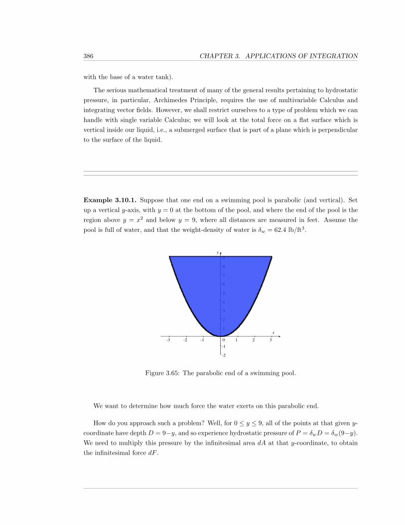
386 CHAPTER 3. APPLICATIONS OF INTEGRATION
with the base of a water tank).
The serious mathematical treatment of many of the general results pertaining to hydrostaticpressure, in particular, Archimedes Principle, requires the use of multivariable Calculus andintegrating vector fields. However, we shall restrict ourselves to a type of problem which we canhandle with single variable Calculus; we will look at the total force on a flat surface which isvertical inside our liquid, i.e., a submerged surface that is part of a plane which is perpendicularto the surface of the liquid.
Example 3.10.1. Suppose that one end on a swimming pool is parabolic (and vertical). Setup a vertical y-axis, with y = 0 at the bottom of the pool, and where the end of the pool is theregion above y = x2 and below y = 9, where all distances are measured in feet. Assume thepool is full of water, and that the weight-density of water is δw = 62.4 lb/ft3.
-3 -2 -1 0 1 2 3
-2
-1
1
2
3
4
5
6
7
8
9
Figure 3.65: The parabolic end of a swimming pool.
We want to determine how much force the water exerts on this parabolic end.
How do you approach such a problem? Well, for 0 ≤ y ≤ 9, all of the points at that given y-coordinate have depth D = 9−y, and so experience hydrostatic pressure of P = δwD = δw(9−y).We need to multiply this pressure by the infinitesimal area dA at that y-coordinate, to obtainthe infinitesimal force dF .
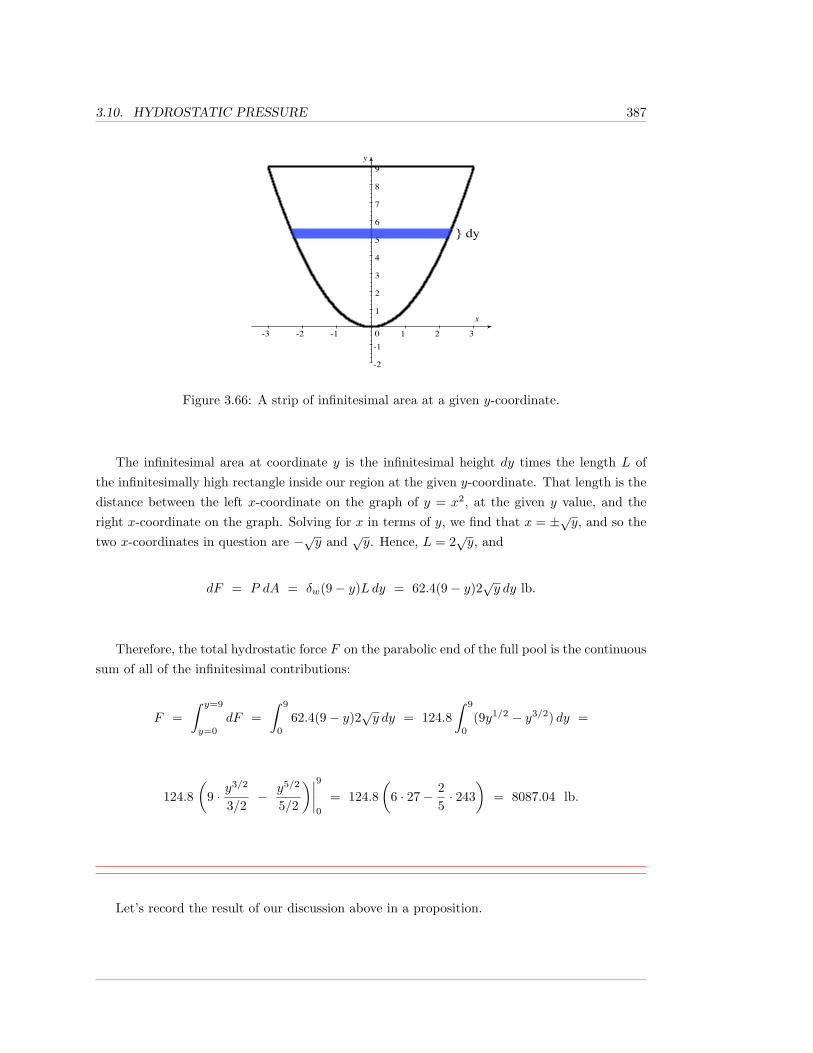
3.10. HYDROSTATIC PRESSURE 387
-3 -2 -1 0 1 2 3
-2
-1
1
2
3
4
5
6
7
8
9
} dy
Figure 3.66: A strip of infinitesimal area at a given y-coordinate.
The infinitesimal area at coordinate y is the infinitesimal height dy times the length L ofthe infinitesimally high rectangle inside our region at the given y-coordinate. That length is thedistance between the left x-coordinate on the graph of y = x2, at the given y value, and theright x-coordinate on the graph. Solving for x in terms of y, we find that x = ±√y, and so thetwo x-coordinates in question are −√y and
√y. Hence, L = 2
√y, and
dF = P dA = δw(9− y)Ldy = 62.4(9− y)2√y dy lb.
Therefore, the total hydrostatic force F on the parabolic end of the full pool is the continuoussum of all of the infinitesimal contributions:
F =∫ y=9
y=0
dF =∫ 9
0
62.4(9− y)2√y dy = 124.8
∫ 9
0
(9y1/2 − y3/2) dy =
124.8(
9 · y3/2
3/2− y5/2
5/2
)∣∣∣∣90
= 124.8(
6 · 27− 25· 243
)= 8087.04 lb.
Let’s record the result of our discussion above in a proposition.
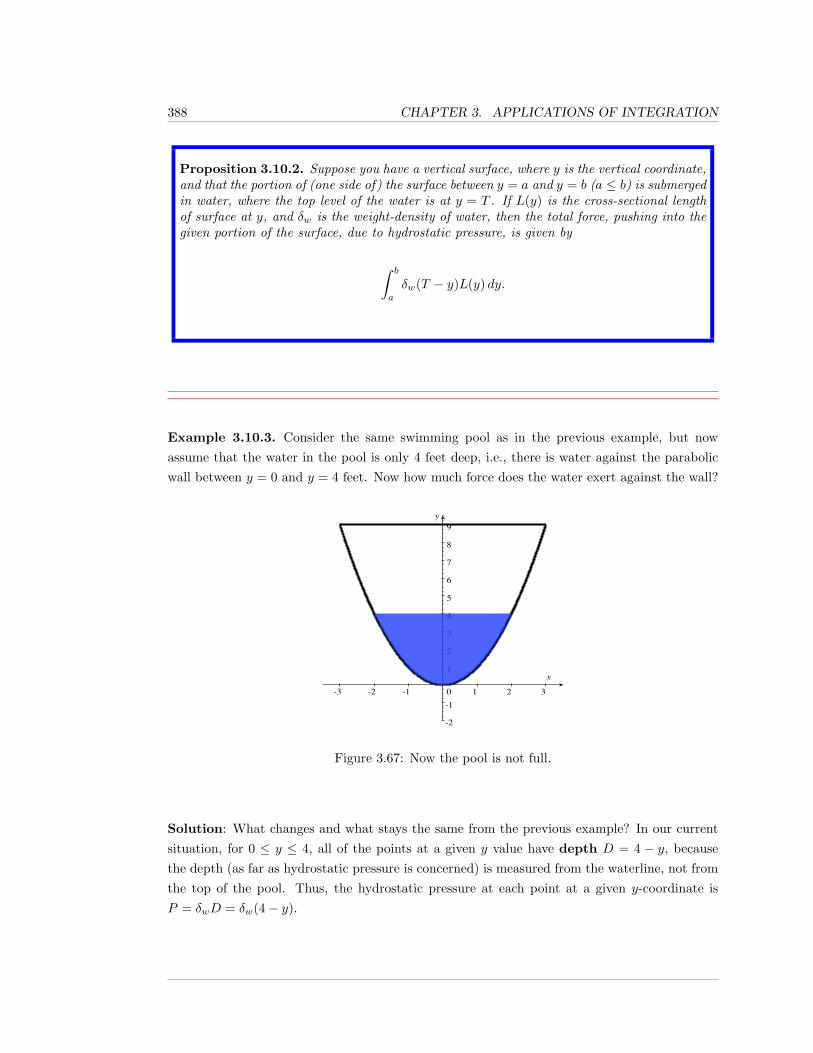
388 CHAPTER 3. APPLICATIONS OF INTEGRATION
Proposition 3.10.2. Suppose you have a vertical surface, where y is the vertical coordinate,and that the portion of (one side of) the surface between y = a and y = b (a ≤ b) is submergedin water, where the top level of the water is at y = T . If L(y) is the cross-sectional lengthof surface at y, and δw is the weight-density of water, then the total force, pushing into thegiven portion of the surface, due to hydrostatic pressure, is given by
∫ b
a
δw(T − y)L(y) dy.
Example 3.10.3. Consider the same swimming pool as in the previous example, but nowassume that the water in the pool is only 4 feet deep, i.e., there is water against the parabolicwall between y = 0 and y = 4 feet. Now how much force does the water exert against the wall?
-3 -2 -1 0 1 2 3
-2
-1
1
2
3
4
5
6
7
8
9
Figure 3.67: Now the pool is not full.
Solution: What changes and what stays the same from the previous example? In our currentsituation, for 0 ≤ y ≤ 4, all of the points at a given y value have depth D = 4 − y, becausethe depth (as far as hydrostatic pressure is concerned) is measured from the waterline, not fromthe top of the pool. Thus, the hydrostatic pressure at each point at a given y-coordinate isP = δwD = δw(4− y).
3.10. HYDROSTATIC PRESSURE 389
The infinitesimal area at coordinate y is still the infinitesimal height dy times the length L
of the infinitesimally high rectangle inside our region at the given y-coordinate. That length isstill L = 2
√y, and so
dF = P dA = δw(4− y)Ldy = 62.4(4− y)2√y dy lb.
The total hydrostatic force F on the parabolic end of the full pool is the continuous sumof all of the infinitesimal contributions, but now there are contributions only for 0 ≤ y ≤ 4.Therefore,
F =∫ y=4
y=0
dF =∫ 4
0
62.4(4− y)2√y dy = 124.8
∫ 4
0
(4y1/2 − y3/2) dy =
124.8(
4 · y3/2
3/2− y5/2
5/2
)∣∣∣∣40
= 124.8(
83· 8− 2
5· 32)
= 1064.96 lb,
which is far less force than we found in the previous example in which the pool was full.
3.10.1 Exercises
Throughout these exercises assume that the weight-density of water is 62.4 lb/ft3 or 9800 N/m3.
1. Suppose that one side of a swimming pool is a flat, vertical rectangular wall of length 12feet and height 10 feet, and the pool is full, i.e., the water is 10 feet deep. Find the totalhydrostatic force on the given wall.
2. Consider the previous exercise.
a. How much force is exerted on the lower half (half, by height) of the wall?
b. How much force is exerted on the upper half of the wall?
c. Explain why one of these values should obviously be larger than the other.
3. Suppose that one side of a swimming pool is a wall which is a flat, vertical isoscelestrapezoid, with height 10 meters, and that the upper parallel side has length 12 meters,and the lower parallel side has length 8 meters. Suppose that the pool is full, i.e., thewater is 10 meters deep. Find the total hydrostatic force on the given wall.
390 CHAPTER 3. APPLICATIONS OF INTEGRATION
4. Consider the previous exercise.
a. How much force is exerted on the lower half (half, by height) of the wall?
b. How much is exerted on the upper half of the wall?
c. Explain why, this time, unlike in Exercise 2, it is not so obvious that one of thesevalues should obviously be larger than the other.
5. Suppose that one side of a tank is a flat, vertical semi-circular wall of radius 6 feet, withthe “big end” up, i.e., the diameter of the semi-circle is at the top of the tank. Supposethat the water is 4 feet deep (that is, the top of the water is 4 feet above the bottom ofthe semicircle).
a. Set this up with y = 0 at the top of the wall. Show that the total hydrostatic forceis given by ∫ −2
−6
62.4(−y)2√
36− y2 dy lb.
b. Evaluate the integral from part a.
6. Suppose now that the semi-circular wall, of radius 6 feet, from the previous problem isupside-down, i.e., the diameter of the semi-circle is at the bottom of the tank. If the waterin the tank is still 4 feet deep, determine the hydrostatic force on the wall.
7. Suppose that one side of a tank is a wall which is a flat, vertical isosceles triangle, with theequal angles at the top, and a vertex at the bottom. Let H be the height of the triangle,and let W be the width at the top of the triangle. Suppose that the tank is full, i.e., thewater is H meters deep. Find the total hydrostatic force on the given wall.
8. Consider the previous exercise.
a. How much force is exerted on the lower half (half, by height) of the wall?
b. How much is exerted on the upper half of the wall?
c. What do you observe about your answers in parts (b) and (c)?
9. Let’s generalize what you should have observed in the previous exercise. Suppose that oneside of a tank is a wall which is flat and vertical. Let y = 0 correspond to the bottom ofthe wall, and y = b correspond to the top. Suppose that the cross-sectional length of thewall is given by L(y) = ky, for some constant k > 0. Suppose the tank is full, so that thetop of the water is also at y = b.
Show that the hydrostatic force on the lower half (half, by height) of the wall is equal tothe hydrostatic force on the upper half.
3.10. HYDROSTATIC PRESSURE 391
10. Consider a vertical end of a swimming pool, as in Example 3.10.1 and Example 3.10.3.Let A be the area of the region R of the vertical end that’s covered with water. Set up avertical y-axis. Then, show that the total hydrostatic force acting on the swimming poolend is equal to δwAD, where δw is the weight-density of water and D is the depth (belowthe waterline) of the y-coordinate of the centroid of R (see Section 3.8).

392 CHAPTER 3. APPLICATIONS OF INTEGRATION
Chapter 4
Understanding Functions viaPolynomials and Power Series
Fundamentally, the question that we address in this chapter is: what does it mean to “knowwhat a function is”?
Do you really know what a function f(x) is if you can’t calculate the value of f , to somedesired accuracy, for each x in the domain of f? Or, another way to look at this is: does yourcalculator know what functions are better than you do? It can calculate values, to the accuracyof the display, of functions like ex, lnx, sinx, and tan−1 x. Can we do the same thing?
However, knowing what a function is goes beyond what your calculator can easily handle.We’d also like to know when one interesting combination of functions is equal to another inter-esting combination of functions, as functions, not just for specific values of the independentvariable; in other words, we’d like to produce identities between functions, and/or recognizewhen we have them.
As we shall see, you can often approximate functions to any desired accuracy by using poly-nomials, and many functions that we use often are equal to power series, basically polynomialswith an infinite number of terms.
Because polynomial functions are so easy to evaluate and manipulate, approximating viapolynomials, and/or representing a function as some sort of never-ending polynomial, is ex-tremely valuable. As you may recall, in Worldwide Differential Calculus, [2], we actually definedthe exponential function exp(x) = ex by using a power series, which made it very easy to derivethe important properties of exp(x), and allowed us to approximate the value of e = exp(1) toany desired accuracy.
Most of the technical details of this chapter are theorems that will appear in the next
393

394 CHAPTER 4. POLYNOMIALS AND POWER SERIES
chapter. Most textbooks place the study of these theorems before the results on polynomialapproximation and power series. Sadly, this seems to lead to many students missing the mostimportant and useful aspects of the theory.
4.1. APPROXIMATING POLYNOMIALS 395
4.1 Approximating Polynomials
In this section, we will discuss approximating polynomials by using just some of their terms/summands.This will also require us to rewrite polynomials, where, instead of using powers of x, we usepowers of (x − a), where a is some fixed value, e.g., powers of (x − 2). As we shall see, thisrewriting is important for approximating well for values of x near a.
Throughout this section, m and n will both denote integers which are greater than, or equalto, zero.
Of course, you know that a polynomial function is a function p(x) defined by a polynomial,e.g.,
p(x) = 4− 2x+ 5x2 + 9x5.
Note that the term polynomial actually refers to the algebraic expression, while polynomialfunction means the function defined by the algebraic expression; this distinction will nevercause us a problem, for we will always be very explicit about the algebraic ways in which wewish to rewrite polynomials, even though the original and rewritten polynomials will, of course,both define the same function.
Using our sigma/summation notation (from Definition 2.1.1), we can write a general poly-nomial, in powers of x, as
p(x) = c0 + c1x+ c2x2 + c3x
3 + · · ·+ cdxd =
d∑k=0
ckxk,
where d is the degree of the polynomial, provided that cd 6= 0. Note that, in the above, formula,we have assumed that x0 = 1, even if x = 0. This is very notational convenient.
We shall adopt the convention that the expression x0 is equal to 1, even when x = 0.
We do this despite the fact that 00 is, in general, undefined. This convention simply savesus from having to write a lot of extra words about what we mean in various formulas, in thespecial case where x = 0.
Much of this section is based on the simple observation:
396 CHAPTER 4. POLYNOMIALS AND POWER SERIES
Proposition 4.1.1. When x is close to 0, higher powers of x are closer to 0. More precisely,if 1 ≤ m < n, and 0 < |x| < 1, then |xn| < |xm|, and limp→∞ |xp| = 0.
So? What does this do for us? It gives us the (imprecise) general principle:
When x is close to 0, a polynomial function p(x) can be approximated “well” by leaving offterms of the form xn, where n is “large”.
We shall make the above general principle more precise in Section 4.3.
Let’s look at an example.
Example 4.1.2. Consider the polynomial function
p(x) = 4− 2x+ 5x2 + 9x5.
You may be used to thinking of the highest-power term 9x5 as the most important term ofthe polynomial and, if x is large in absolute value, then that’s certainly correct. But, when x
is close to 0, x5 will be very small, even after multiplying by 9. The point is: when x is closeto 0, the 0-th degree term, 4, is the most important, −2x is the second most important term,and 5x2 is third most important; the 9x5 term is the least important if x is close enough to 0.
How close does x need to be to 0 to make the lower-degree terms larger in absolute valuethan the higher-degree terms? That depends on the precise coefficients in p(x), and we willaddress such questions in a more general context in Section 4.3. For now, we’re going to plugin some numbers and look at the approximations that we obtain when we omit the terms of“large” degree.
However, before we start plugging in numbers, let’s adopt the notation that pn(x) means thesum of all of the terms of p(x), from the constant term up to the xn term (even if that term ismissing, i.e., has a zero coefficient).
Hence,
p0(x) = 4, p1(x) = 4− 2x, p2(x) = 4− 2x+ 5x2, p3(x) = 4− 2x+ 5x2,
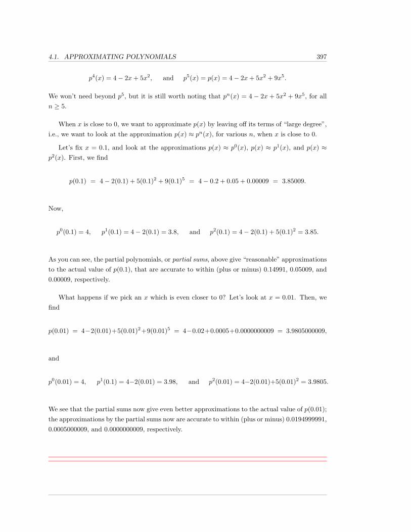
4.1. APPROXIMATING POLYNOMIALS 397
p4(x) = 4− 2x+ 5x2, and p5(x) = p(x) = 4− 2x+ 5x2 + 9x5.
We won’t need beyond p5, but it is still worth noting that pn(x) = 4 − 2x + 5x2 + 9x5, for alln ≥ 5.
When x is close to 0, we want to approximate p(x) by leaving off its terms of “large degree”,i.e., we want to look at the approximation p(x) ≈ pn(x), for various n, when x is close to 0.
Let’s fix x = 0.1, and look at the approximations p(x) ≈ p0(x), p(x) ≈ p1(x), and p(x) ≈p2(x). First, we find
p(0.1) = 4− 2(0.1) + 5(0.1)2 + 9(0.1)5 = 4− 0.2 + 0.05 + 0.00009 = 3.85009.
Now,
p0(0.1) = 4, p1(0.1) = 4− 2(0.1) = 3.8, and p2(0.1) = 4− 2(0.1) + 5(0.1)2 = 3.85.
As you can see, the partial polynomials, or partial sums, above give “reasonable” approximationsto the actual value of p(0.1), that are accurate to within (plus or minus) 0.14991, 0.05009, and0.00009, respectively.
What happens if we pick an x which is even closer to 0? Let’s look at x = 0.01. Then, wefind
p(0.01) = 4−2(0.01)+5(0.01)2+9(0.01)5 = 4−0.02+0.0005+0.0000000009 = 3.9805000009,
and
p0(0.01) = 4, p1(0.1) = 4−2(0.01) = 3.98, and p2(0.01) = 4−2(0.01)+5(0.01)2 = 3.9805.
We see that the partial sums now give even better approximations to the actual value of p(0.01);the approximations by the partial sums now are accurate to within (plus or minus) 0.0194999991,0.0005000009, and 0.0000000009, respectively.
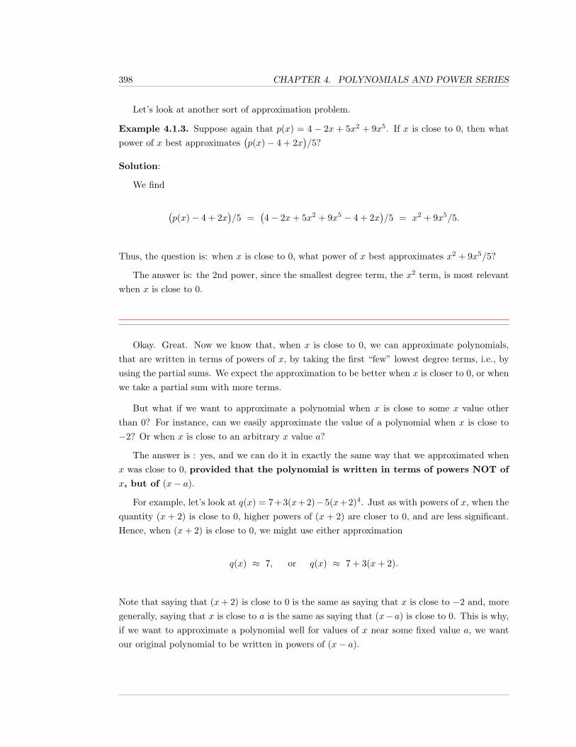
398 CHAPTER 4. POLYNOMIALS AND POWER SERIES
Let’s look at another sort of approximation problem.
Example 4.1.3. Suppose again that p(x) = 4 − 2x + 5x2 + 9x5. If x is close to 0, then whatpower of x best approximates
(p(x)− 4 + 2x
)/5?
Solution:
We find
(p(x)− 4 + 2x
)/5 =
(4− 2x+ 5x2 + 9x5 − 4 + 2x
)/5 = x2 + 9x5/5.
Thus, the question is: when x is close to 0, what power of x best approximates x2 + 9x5/5?
The answer is: the 2nd power, since the smallest degree term, the x2 term, is most relevantwhen x is close to 0.
Okay. Great. Now we know that, when x is close to 0, we can approximate polynomials,that are written in terms of powers of x, by taking the first “few” lowest degree terms, i.e., byusing the partial sums. We expect the approximation to be better when x is closer to 0, or whenwe take a partial sum with more terms.
But what if we want to approximate a polynomial when x is close to some x value otherthan 0? For instance, can we easily approximate the value of a polynomial when x is close to−2? Or when x is close to an arbitrary x value a?
The answer is : yes, and we can do it in exactly the same way that we approximated whenx was close to 0, provided that the polynomial is written in terms of powers NOT of
x, but of (x− a).
For example, let’s look at q(x) = 7+3(x+2)−5(x+2)4. Just as with powers of x, when thequantity (x + 2) is close to 0, higher powers of (x + 2) are closer to 0, and are less significant.Hence, when (x+ 2) is close to 0, we might use either approximation
q(x) ≈ 7, or q(x) ≈ 7 + 3(x+ 2).
Note that saying that (x+ 2) is close to 0 is the same as saying that x is close to −2 and, moregenerally, saying that x is close to a is the same as saying that (x− a) is close to 0. This is why,if we want to approximate a polynomial well for values of x near some fixed value a, we wantour original polynomial to be written in powers of (x− a).
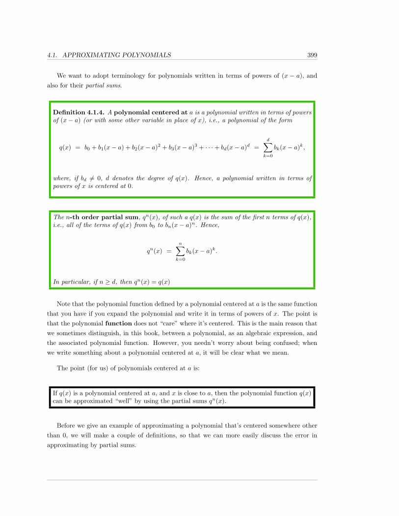
4.1. APPROXIMATING POLYNOMIALS 399
We want to adopt terminology for polynomials written in terms of powers of (x − a), andalso for their partial sums.
Definition 4.1.4. A polynomial centered at a is a polynomial written in terms of powersof (x− a) (or with some other variable in place of x), i.e., a polynomial of the form
q(x) = b0 + b1(x− a) + b2(x− a)2 + b3(x− a)3 + · · ·+ bd(x− a)d =d∑k=0
bk(x− a)k,
where, if bd 6= 0, d denotes the degree of q(x). Hence, a polynomial written in terms ofpowers of x is centered at 0.
The n-th order partial sum, qn(x), of such a q(x) is the sum of the first n terms of q(x),i.e., all of the terms of q(x) from b0 to bn(x− a)n. Hence,
qn(x) =n∑k=0
bk(x− a)k.
In particular, if n ≥ d, then qn(x) = q(x)
Note that the polynomial function defined by a polynomial centered at a is the same functionthat you have if you expand the polynomial and write it in terms of powers of x. The point isthat the polynomial function does not “care” where it’s centered. This is the main reason thatwe sometimes distinguish, in this book, between a polynomial, as an algebraic expression, andthe associated polynomial function. However, you needn’t worry about being confused; whenwe write something about a polynomial centered at a, it will be clear what we mean.
The point (for us) of polynomials centered at a is:
If q(x) is a polynomial centered at a, and x is close to a, then the polynomial function q(x)can be approximated “well” by using the partial sums qn(x).
Before we give an example of approximating a polynomial that’s centered somewhere otherthan 0, we will make a couple of definitions, so that we can more easily discuss the error inapproximating by partial sums.
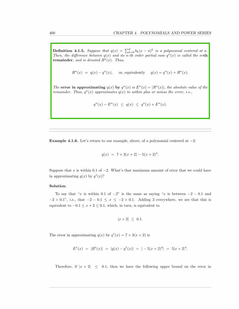
400 CHAPTER 4. POLYNOMIALS AND POWER SERIES
Definition 4.1.5. Suppose that q(x) =∑dk=0 bk(x − a)k is a polynomial centered at a.
Then, the difference between q(x) and its n-th order partial sum qn(x) is called the n-thremainder, and is denoted Rn(x). Thus,
Rn(x) = q(x)− qn(x), or, equivalently q(x) = qn(x) +Rn(x).
The error in approximating q(x) by qn(x) is En(x) = |Rn(x)|, the absolute value of theremainder. Thus, qn(x) approximates q(x) to within plus or minus the error, i.e.,
qn(x)− En(x) ≤ q(x) ≤ qn(x) + En(x).
Example 4.1.6. Let’s return to our example, above, of a polynomial centered at −2:
q(x) = 7 + 3(x+ 2)− 5(x+ 2)4.
Suppose that x is within 0.1 of −2. What’s that maximum amount of error that we could havein approximating q(x) by q1(x)?
Solution:
To say that “x is within 0.1 of −2” is the same as saying “x is between −2 − 0.1 and−2 + 0.1”, i.e., that −2 − 0.1 ≤ x ≤ −2 + 0.1. Adding 2 everywhere, we see that this isequivalent to −0.1 ≤ x+ 2 ≤ 0.1, which, in turn, is equivalent to
|x+ 2| ≤ 0.1.
The error in approximating q(x) by q1(x) = 7 + 3(x+ 2) is
E1(x) = |R1(x)| = |q(x)− q1(x)| = | − 5(x+ 2)4| = 5|x+ 2|4.
Therefore, if |x + 2| ≤ 0.1, then we have the following upper bound on the error in
4.1. APPROXIMATING POLYNOMIALS 401
approximating q(x) by q1(x):
E1(x) = 5|x+ 2|4 ≤ 5(0.1)4 = 0.0005.
It is important to note that this is an upper bound on the error in the approximation,given that all that we know about x is that |x + 2| ≤ 0.1. Of course, if we know that someparticular x is even closer to −2, then the error E1(x) will be smaller than 0.0005.
At this point, we know that, when x is close to a, we can approximate a polynomial q(x),which is in terms of powers of (x−a), by using the partial sums qn(x). But what do we do if weare given a polynomial centered at one point, say, centered at 0, and we want to approximatethe values of the polynomial function when x is near some other point a 6= 0?
What we need to be able to do is start with a polynomial function p(x), of degree d, andfigure out how to rewrite p(x) as a polynomial q(x) centered at any point a that we desire. Thatis, given p(x) and a, we need to be able to produce the coefficients bk so that
p(x) = b0 + b1(x− a) + b2(x− a)2 + b3(x− a)3 + · · ·+ bd(x− a)d =d∑k=0
bk(x− a)k.
Before we describe what happens generally, let’s look at an example.
Example 4.1.7. Suppose that, once again, p(x) = 4− 2x+ 5x2 + 9x5, and we want to approx-imate p(x) by some lower-degree polynomial, so that the approximation is good when x is closeto 1.
What we need to do is rewrite p(x) as a polynomial q(x), which is centered at 1, and thenuse the partial sums of q(x) for our approximations. Thus, we want to find b0, b1, b2, b3, b4,and b5 so that
b0 + b1(x− 1) + b2(x− 1)2 + b3(x− 1)3 + b4(x− 1)4 + b5(x− 1)5 = p(x). (4.1)
We could (but won’t) approach this in a purely algebraic fashion: you expand all of the terms
402 CHAPTER 4. POLYNOMIALS AND POWER SERIES
on the left, collect the terms with the same powers of x, and match the coefficient of each xk onthe left with the coefficient of xk in p(x). The coefficients on the left will involve all of the bk,and you will end up with 6 (linear) equations and 6 unknowns. These equations will actuallybe easy to solve: you first find b5, then b4 is easy to determine after that, then b3, and so on.
However, Calculus gives us a much easier, faster way to determine the bk. First, plug inx = 1 on both sides of Formula 4.1, and note that all of the powers (x − 1)k, where k ≥ 1,become 0. Therefore, we obtain quickly that
b0 = p(1).
Now, differentiate each side of Formula 4.1 to obtain
b1 + 2b2(x− 1) + 3b3(x− 1)2 + 4b4(x− 1)3 + 5b5(x− 1)4 = p′(x) (4.2)
and, once again, plug x = 1 into both sides of the equation; all of the powers of (x − 1) are 0,and we find
b1 = p′(1).
You may guess at this point that bk always equals p(k)(1), the k-th derivative of p at 1. This isnot correct.
Differentiate again (differentiate Formula 4.2), to obtain
2b2 + 2 · 3b3(x− 1) + 3 · 4b4(x− 1)2 + 4 · 5b5(x− 1)3 = p′′(x) (4.3)
and plug in x = 1 to find
b2 =p′′(1)
2.
Hmmmm...what is the pattern here? Let’s differentiate more times, and always plug in x = 1.You’ll see what happens. We find:
2 · 3b3 + 2 · 3 · 4b4(x− 1) + 3 · 4 · 5b5(x− 1)2 = p′′′(x),
2 · 3 · 4b4 + 2 · 3 · 4 · 5b5(x− 1) = p(4)(x),
4.1. APPROXIMATING POLYNOMIALS 403
2 · 3 · 4 · 5b5 = p(5)(x),
and so
b3 =p′′′(1)
3!, b4 =
p(4)(1)4!
, and b5 =p(5)(1)
5!,
where, for n ≥ 1, p(n) denotes the n-th derivative of p, and n! = 1 · 2 · 3 · · · ·n is n factorial.For n = 0, there are special definitions; p(0) is the 0-th derivative of p, and so is just p itself (pdifferentiated zero times), while 0! is defined to be 1.
With these notations, what we have seen is that, for all k, we have the general formula
bk =p(k)(1)k!
.
For our particular p(x) = 4− 2x+ 5x2 + 9x5, we find
p′(x) = −2 + 10x+ 5 · 9x4, p′′(x) = 10 + 4 · 5 · 9x3, p(3)(x) = 3 · 4 · 5 · 9x2,
p(4)(x) = 2 · 3 · 4 · 5 · 9x, and p(5)(x) = 2 · 3 · 4 · 5 · 9.
Therefore,
b0 = p(1) = 16, b1 = p′(1) = 53, b2 =p′′(1)
2= 95, b3 =
p′′′(1)2 · 3
= 90,
b4 =p(4)(1)2 · 3 · 4
= 45, and b5 =p(5)(1)
2 · 3 · 4 · 5= 9.
Finally, we findp(x) = 4− 2x+ 5x2 + 9x5 =
16 + 53(x− 1) + 95(x− 1)2 + 90(x− 1)3 + 45(x− 1)4 + 9(x− 1)5.
So, how do you produce a reasonable approximation of p(x), when x is close to 1? Use thepartial sums of the polynomial centered at 1, e.g.,
16 + 53(x− 1) or 16 + 53(x− 1) + 95(x− 1)2
would provide reasonable lower-degree approximations of p(x), when x is close to 1.
404 CHAPTER 4. POLYNOMIALS AND POWER SERIES
The process that we went through in the above example works in general. We conclude:
Proposition 4.1.8. Suppose that p(x) is a polynomial function of degree d, and that a isa fixed number. Then, there is a unique polynomial, of degree d,
q(x) =d∑k=0
bk(x− a)k,
centered at a, such that there is an equality of functions p(x) = q(x); that polynomial is theone which has coefficients given by
bk =p(k)(a)k!
.
Example 4.1.9. Rewrite the polynomial p(x) = (x− 2)3 as a polynomial centered at −1, anduse the 2nd partial sum of this new polynomial to approximate p(−0.9).
Solution:
In order to use Proposition 4.1.8, we need to calculate the derivatives of p at −1. We find
p′(x) = 3(x− 2)2, p′′(x) = 6(x− 2), and p′′′(x) = 6,
and sop(−1) = −27, p′(−1) = 27, p′′(−1) = −18, and p′′′(−1) = 6.
Therefore, Proposition 4.1.8 tells us that
(x− 2)3 = −27 + 27(x+ 1) +−18
2(x+ 1)2 +
66
(x+ 1)3 =
−27 + 27(x+ 1)− 9(x+ 1)2 + (x+ 1)3.
4.1. APPROXIMATING POLYNOMIALS 405
The approximation
(x− 2)3 ≈ −27 + 27(x+ 1)− 9(x+ 1)2,
applied to x = −0.9 yields
p(−0.9) = (−2.9)3 ≈ −27 + 27(0.1)− 9(0.1)2 = −24.39.
The actual value of (−2.9)3 is −24.389; so our approximation is pretty good.
4.1.1 Exercises
In Exercises 1 through 6, you are given a polynomial p(x), centered at some a, and
values x0 near, or equal to, the center. For each x0, determine p(x0), and the values
of the 1st and 2nd order partial sums of p(x), evaluated at x0. In each case, find the
error in approximating p(x0) by the 1st and 2nd partial sums.
1. p(x) = 4− 3x+ 5x2 − 9x3 + 100x4; x0 = 0, 0.1, 0.01, −0.001.
2. p(x) = 4− 3(x+ 2) + 5(x+ 2)2− 9(x+ 2)3 + 100(x+ 2)4; x0 = −2, −1.9, −1.99, −2.001.
3. p(x) = 7 + (x− 1) + 12(x− 1)2 − 15(x− 1)6; x0 = 1, 1.1, 1.01, 0.999.
4. p(x) = 7 + x+ 12x2 − 15x6; x0 = 0, 0.1, 0.01, −0.001.
5. p(x) = 1 + x+ x2 + x3 + x4 + x5; x0 = 0, −0.01, 0.001.
6. p(x) = 1 + (x−π) + (x−π)2 + (x−π)3 + (x−π)4 + (x−π)5; x0 = π, π−0.01, π+ 0.001.
7. Let p(x) = 4 − 3x + 5x2 − 9x3 + 100x4. When x is close to 0, what power of x bestapproximates
15(p(x)− 4 + 3x
)?
8. Let p(x) = 4− 3(x+ 2) + 5(x+ 2)2− 9(x+ 2)3 + 100(x+ 2)4. When x is close to −2, whatpower of (x+ 2) best approximates
15(p(x)− 4 + 3(x+ 2)
)?
406 CHAPTER 4. POLYNOMIALS AND POWER SERIES
9. Let p(x) = 7 + (x− 1) + 12(x− 1)2 − 15(x− 1)6. When x is close to 1, what polynomialof the form c(x− 1)n best approximates p(x)− 7− (x− 1)?
10. Let p(x) = 7 + (x− 1) + 12(x− 1)2 − 15(x− 1)6. When x is close to 1, what polynomialof the form c(x− 1)n best approximates the derivative
[p(x)− 7− (x− 1)
]′?In each of Exercises 11 through 15, rewrite the polynomial q(x) as a polynomial
centered at the given a.
11. q(x) = x2 + 5x+ 6, a = −2.
12. q(x) = (x+ 2)3 − (x+ 2) + 1, a = 2.
13. q(x) = x3 + 15x2 + 75x+ 125, a = 5.
14. q(x) = 1 + x+ 2x2 + 3x3 + 4x4, a = 1.
15. q(x) = 1− x+ 2x2 − 3x3 + 4x4, a = 1.
In each of Exercises 16 through 20, use the (re-centered) 1st order partial sum from
your answers to Exercises 11 through 15 to approximate q(x) at the given value.
16. Approximate q(x) = x2 + 5x+ 6 at x = −2.1.
17. Approximate q(x) = (x+ 2)3 − (x+ 2) + 1 at x = 2.05.
18. Approximate q(x) = x3 + 15x2 + 75x+ 125 at x = 4.99.
19. Approximate q(x) = 1 + x+ 2x2 + 3x3 + 4x4 at x = 1.1.
20. Approximate q(x) = 1− x+ 2x2 − 3x3 + 4x4 at x = 1.1.
In Exercises 21 through 25, use the method from Example 4.1.6 to calculate an
upper bound on the error in approximating q(x) by qd−1(x), where d is the degree
of q, for x values within the given amount of the center.
21. q(x) = 3 + 4(x+ 2)− 6(x+ 2)2, x is within 0.2 of −2.
22. q(x) = 4x4 + 3x3 + 2x2 + x+ 1, x is within 0.1 of 0.
23. q(x) = 5(x− 3)5 − 7(x− 3), x is within 0.01 of 3.
24. q(x) = 6(x− 1)3 − 5(x− 1) + 7, x is within 0.05 0f 1.
4.1. APPROXIMATING POLYNOMIALS 407
25. q(x) = 12(x+ 4)4 + (x+ 4)3 − (x+ 4)2 + (x+ 4), x is within 0.3 of −4.
26. a. Let p(x) be a polynomial (centered at 0) which contains only even powers of x.Suppose b0, ..., bd are the coefficients of p(x) centered at a and that c0, ..., cd are thecoefficients of p(x) centered at −a. Prove that bi = ci when i is even, and bi = −ciwhen i is odd.
b. State and prove a similar conclusion when p(x) contains only odd powers of x.
408 CHAPTER 4. POLYNOMIALS AND POWER SERIES
4.2 Approximation of Functions by Polynomials
In the previous section, we discussed approximating polynomials p(x), centered at some point a,for values of x close to a, by using the first few lowest-degree terms, i.e., by using partial sums.
In this section, our goal is to investigate approximating a non-polynomial function f(x), byusing a polynomial function p(x) and, if we want the approximation to be good for x near a, thenwe will use a polynomial which is centered at a. Why do this? Because polynomials are our
friends; we can easily evaluate polynomials by hand (if we have to), because all that’s involvedis raising to powers, multiplying by constants, and adding (or subtracting). We understandpolynomials, and if we can use them to accurately approximate other functions, then we cansay, in some serious sense, that we understand the functions being approximated.
In this section, we will give the intuitive idea, and look at examples. In the next section, wewill investigate how you can place some rigorous bounds on how good/bad the approximationmay be.
Suppose that we have two functions f(x) and p(x), which are both n times differentiable,for some integer n ≥ 0. We’re thinking of f(x) as a non-polynomial function, and of p(x) as apolynomial centered at a, but, for now, they could be any two functions which are differentiableenough.
If we want p(x) to provide a good approximation of f(x), when x is close to a, what shouldwe want to be true? Well, first of all, we can require that at a, f and g have the same value,i.e., require that f(a) = p(a); to make this fit in with what we will see later, we also say that fand p have the same 0-th derivative at a. This is equivalent to saying that the graphs of f andp intersect at the point (a, f(a)) = (a, p(a)). As f and g are differentiable, they’re continuous,and so, requiring them to be equal at a forces them to not be too far apart if x is close to a.But can we do better?
How about if we continue to require f(a) = p(a), and also require that f and p are changingat the same rate at x = a? This certainly seems like it should force f and p to be close toeach other for x near a. This new condition is simply that f ′(a) = p′(a), and, combined withrequiring that f(a) = p(a), means that the graphs of y = f(x) and y = p(x) have the sametangent lines at the point (a, f(a)) = (a, p(a)).
But two graphs which intersect at a point, and have the same tangent line there, may nothave the same concavity. Wouldn’t requiring that the two graphs have the same tangent lineand concavity at the point (a, f(a)) = (a, p(a)) force the values of the two functions to be even
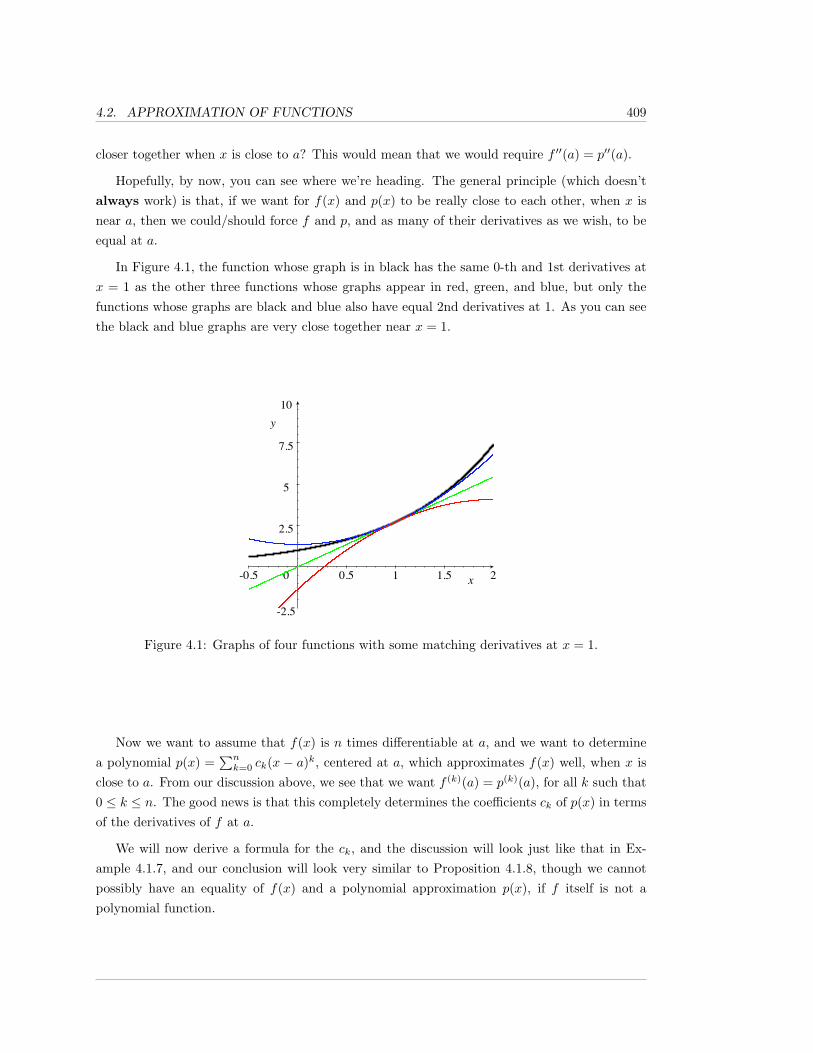
4.2. APPROXIMATION OF FUNCTIONS 409
closer together when x is close to a? This would mean that we would require f ′′(a) = p′′(a).
Hopefully, by now, you can see where we’re heading. The general principle (which doesn’talways work) is that, if we want for f(x) and p(x) to be really close to each other, when x isnear a, then we could/should force f and p, and as many of their derivatives as we wish, to beequal at a.
In Figure 4.1, the function whose graph is in black has the same 0-th and 1st derivatives atx = 1 as the other three functions whose graphs appear in red, green, and blue, but only thefunctions whose graphs are black and blue also have equal 2nd derivatives at 1. As you can seethe black and blue graphs are very close together near x = 1.
-0.5 0 0.5 1 1.5 2
-2.5
2.5
5
7.5
10
Figure 4.1: Graphs of four functions with some matching derivatives at x = 1.
Now we want to assume that f(x) is n times differentiable at a, and we want to determinea polynomial p(x) =
∑nk=0 ck(x − a)k, centered at a, which approximates f(x) well, when x is
close to a. From our discussion above, we see that we want f (k)(a) = p(k)(a), for all k such that0 ≤ k ≤ n. The good news is that this completely determines the coefficients ck of p(x) in termsof the derivatives of f at a.
We will now derive a formula for the ck, and the discussion will look just like that in Ex-ample 4.1.7, and our conclusion will look very similar to Proposition 4.1.8, though we cannotpossibly have an equality of f(x) and a polynomial approximation p(x), if f itself is not apolynomial function.
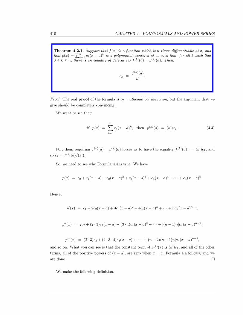
410 CHAPTER 4. POLYNOMIALS AND POWER SERIES
Theorem 4.2.1. Suppose that f(x) is a function which is n times differentiable at a, andthat p(x) =
∑nk=0 ck(x − a)k is a polynomial, centered at a, such that, for all k such that
0 ≤ k ≤ n, there is an equality of derivatives f (k)(a) = p(k)(a). Then,
ck =f (k)(a)k!
.
Proof. The real proof of the formula is by mathematical induction, but the argument that wegive should be completely convincing.
We want to see that:
if p(x) =n∑k=0
ck(x− a)k, then p(k)(a) = (k!)ck. (4.4)
For, then, requiring f (k)(a) = p(k)(a) forces us to have the equality f (k)(a) = (k!)ck, andso ck = f (k)(a)/(k!).
So, we need to see why Formula 4.4 is true. We have
p(x) = c0 + c1(x− a) + c2(x− a)2 + c3(x− a)3 + c4(x− a)4 + · · ·+ cn(x− a)n.
Hence,
p′(x) = c1 + 2c2(x− a) + 3c3(x− a)2 + 4c4(x− a)3 + · · ·+ ncn(x− a)n−1,
p′′(x) = 2c2 + (2 · 3)c3(x− a) + (3 · 4)c4(x− a)2 + · · ·+ [(n− 1)n]cn(x− a)n−2,
p′′′(x) = (2 · 3)c3 + (2 · 3 · 4)c4(x− a) + · · ·+ [(n− 2)(n− 1)n]cn(x− a)n−3,
and so on. What you can see is that the constant term of p(k)(x) is (k!)ck, and all of the otherterms, all of the positive powers of (x − a), are zero when x = a. Formula 4.4 follows, and weare done.
We make the following definition.
4.2. APPROXIMATION OF FUNCTIONS 411
Definition 4.2.2. Suppose that f(x) is a function which is n times differentiable at a.Then, the polynomial
Tnf (x; a) =n∑k=0
f (k)(a)k!
(x− a)k =
f(a) + f ′(a)(x− a) +f ′′(a)
2!(x− a)2 +
f ′′′(a)3!
(x− a)3 + · · ·+ f (n)(a)n!
(x− a)n
is called the n-th order Taylor polynomial of f , centered at a.
When a = 0, we write simply Tnf (x) in place of Tnf (x; 0), and refer to the polynomial
Tnf (x) =n∑k=0
f (k)(0)k!
xk =
f(0) + f ′(0)x+f ′′(0)
2!x2 +
f ′′′(0)3!
x3 + · · ·+ f (n)(0)n!
xn
as the n-th order Maclaurin polynomial of f .
Remark 4.2.3. We want to emphasize that, for all n, Tnf (a; a) = f(a); that is, the Taylorpolynomials always give the actual value of f at x = a.
Note that the n-th order Taylor polynomial will have degree n, provided that f (n)(a) 6= 0; forthis reason, the n-th order Taylor polynomial is sometimes referred to as the degree n Taylor
polynomial, without worrying about whether or not f (n)(a) is zero.
The point of our discussion up to this point is that:
We expect that, for n big enough, Tnf (x; a) approximates f(x) well, when x is near a.
Note that our previous discussion does not prove that for n big enough, Tnf (x; a) approxi-mates f(x) well, for x near a; we will discuss bounds on the error in the approximation in the
412 CHAPTER 4. POLYNOMIALS AND POWER SERIES
next section. In the remainder of this section, we will calculate some specific Taylor/Maclaurinpolynomials, and compare the approximations that we get from them with the “actual values”of f(x) that we get from calculators. This is somewhat circular, since modern computers andscientific calculators, with floating point units, use polynomial approximation to give you highlyaccurate results.
Remark 4.2.4. Note that the 1st order Taylor polynomial T 1f (x; a) = f(a) + f ′(a)(x − a),
centered at a, is precisely the linearization of f at a, Lf (x; a), which we discussed in [2]. Hence,the approximation
f(x) ≈ T 1f (x; a)
is the linear approximation of f(x), when x is close to a.
As we shall see, using Taylor polynomials of order higher than 1 typically yields a betterapproximation than you obtain by using merely the linearization.
Example 4.2.5. Suppose that f(x) = ex. Let’s find Tnf (x), the n-th order Maclaurin poly-nomial of f , and use the 1st and 3rd order Maclaurin polynomials to approximate e0.1. we’llcompare these approximations with the calculator value of e0.1.
The coefficient ck of the xk term in Tnf (x) is ck = f (k)(0)/(k!). So, we need all of thederivatives of f(x) at 0. But all of the derivatives of ex are ex, which has value 1 when x = 0.Therefore, ck = 1/(k!), and the n-th order Maclaurin polynomial of ex is
Tnf (x) =n∑k=0
xk
k!= 1 + x+
x2
2!+x3
3!+ · · ·+ xn
n!.
In a way, this should be very unsurprising; in [2], we defined exp(x) = ex to be the limitof the polynomials
Tnf (x) = 1 + x+x2
2!+x3
3!+ · · ·+ xn
n!.
This leads to a general question which we will address in later sections: when is a function f(x)the limit, as n→∞, of its Taylor polynomials Tnf (x)?
For now, however, we just want to investigate how well T 1f (0.1) and T 3
f (0.1) approximatee0.1 (where, in this section, we are going to rely on our calculators for highly accurate values).
4.2. APPROXIMATION OF FUNCTIONS 413
We shall use an equality sign in quotes to denote “equal, according to the full precision of (our)calculators”.
Your calculator should tell you that
e0.1 “ = ” 1.10517091808,
and we find that
T 1f (0.1) = 1 + 0.1 = 1.1,
while
T 3f (0.1) = 1 + 0.1 +
(0.1)2
2!+
(0.1)3
3!= 1.1051666.
As you can see, the approximation by T 1f is fairly good, but the approximation by T 3
f ismuch better.
Before we go on, it will be convenient to adopt some new notation. Rather than write then-th order Taylor polynomial for arbitrary n, it’s nice to use some notation which implies thatthere is no particular n at which we need to stop. Thus, for example, when f(x) = ex, ratherthan writing that, for all n,
Tnf (x) =n∑k=0
xk
k!= 1 + x+
x2
2!+x3
3!+ · · ·+ xn
n!,
we instead write
Tf (x) = T∞f (x) =∞∑k=0
xk
k!= 1 + x+
x2
2!+x3
3!+ · · · .
We use the notations Tf (x) and T∞f (x) interchangeably. We are not claiming (yet!) thatthis infinite sum defines a function. For now, it is formal notation that simply indicates, forarbitrarily large n, what Tnf (x) is.
More generally, we make the definition:
414 CHAPTER 4. POLYNOMIALS AND POWER SERIES
Definition 4.2.6. A power series, centered at a, is a formal algebraic expression
∞∑k=0
ck(x− a)k = c0 + c1(x− a) + c2(x− a)2 + c3(x− a)3 + · · · ,
where the ck are constants.
Suppose that f(x) is a function which is infinitely differentiable at a, i.e., such that then-th derivative f (n)(a) exists for all n. Then, the power series Tf (x; a) = T∞f (x; a), centeredat a, given by
Tf (x; a) = T∞f (x; a) =∞∑k=0
f (k)(a)k!
(x− a)k =
f(a) + f ′(a)(x− a) +f ′′(a)
2!(x− a)2 +
f ′′′(a)3!
(x− a)3 + · · ·
is the Taylor series of f , centered at a; when a = 0, this is also referred to as theMaclaurin series of f .
Remark 4.2.7. Once we have the notion of a Taylor series, it is natural to think of the n-th
order Taylor polynomial as the n-th order partial sum of the Taylor series.
We also want to state again that, at this point, we have not defined power series functions.Just as there is a difference between a polynomial as an algebraic object and as a polynomialfunction, there is a difference between a power series as an algebraic object and as a function(assuming that we can even make sense of the infinite sum as a function).
Example 4.2.8. Find the Taylor series for f(x) = sinx, centered at π/2, and use the firsttwo non-zero terms to estimate sin(1.5). Compare your estimate with the calculator value ofsin(1.5).
Solution: First, it is important that all angles are in radians, as is always the case in a Calculuscourse, unless you are explicitly told otherwise.
4.2. APPROXIMATION OF FUNCTIONS 415
The Taylor series for f(x), centered at π/2 is the power series
Tf
(x;π
2
)=
∞∑k=0
ck
(x− π
2
)k= c0 + c1
(x− π
2
)+ c2
(x− π
2
)2
+ c3
(x− π
2
)3
+ · · · ,
where ck =f (k)(π2 )k!
.
Thus, as is always the case when finding Taylor series, the problem boils down to calculatingf (k)(a), which here is f (k)(π2 ), for all k.
The derivatives of sine repeat every four times you take a derivative:
f(x) = sinx, f ′(x) = cosx, f ′′(x) = − sinx, f ′′′(x) = − cosx, f (4)(x) = sinx,
and, now that we’re back at sinx, the derivatives just keep cycling. Therefore, the derivatives(including the 0-th), evaluated at a = π/2, are
1, 0, −1, 0, 1, 0, −1, 0, 1, 0, −1, 0, . . .
and so, the Taylor series, centered at π/2 is
Tf
(x;π
2
)=
1 + 0(x− π
2
)− 1
2!
(x− π
2
)2
+ 0(x− π
2
)3
+14!
(x− π
2
)4
+ 0(x− π
2
)5
− 16!
(x− π
2
)6
+ · · · =
1− 12!
(x− π
2
)2
+14!
(x− π
2
)4
− 16!
(x− π
2
)6
+18!
(x− π
2
)8
− 110!
(x− π
2
)10
+ · · · .
Hopefully, you can see the pattern here. We have only the even powers of(x− π
2
)and, for
each term, we divide by a factorial that matches the exponent, and the sign alternates between+ and −.
For many purposes, the formula above for Tf(x; π2
), in which the pattern is clear, is good
416 CHAPTER 4. POLYNOMIALS AND POWER SERIES
enough. However, frequently, we want to write a formula for ck, regardless of what k is, so thatwe can write one “nice-looking” summation formula for the power series. But, in some cases,like our current one, we don’t need to produce a formula for every ck; we really only need aformula for the coefficients of the non-zero terms. In this example, the non-zero terms are theeven-powered terms, and we would like a formula for c2k, where k can be any integer ≥ 0, andthen we will use a summation that runs through only the even powers of
(x− π
2
)in the first
place:
Tf
(x;π
2
)=
∞∑k=0
c2k
(x− π
2
)2k
=
c0 + c2
(x− π
2
)2
+ c4
(x− π
2
)4
+ c6
(x− π
2
)6
+ c8
(x− π
2
)8
+ c10
(x− π
2
)10
+ · · · .
So, now the question is: can we write a nice formula for c2k? Let’s see, we have
c2·0 = c0 = 1, c2·1 = c2 = − 12!, c2·2 = c4 =
14!
c2·3 = c6 = − 16!, c2·4 = c8 =
18!, . . . .
We can see that the pattern is that
c2k = ± 1(2k)!
,
where the sign alternates from one even-subscripted coefficient to the next, but can we writean algebraic formula for this alternating sign? Yes. The standard “trick” for this is to look at(−1)k or (−1)k+1 = (−1)k−1; for (−1)k equals 1 when k is even, and −1 when k is odd, while,on the other hand, (−1)k+1 equals 1 when k is odd, and −1 when k is even.
Therefore, looking at our coefficients, we see that we want
c2k = (−1)k1
(2k)!,
so that
Tf
(x;π
2
)=
∞∑k=0
(−1)k1
(2k)!
(x− π
2
)2k
=
1− 12!
(x− π
2
)2
+14!
(x− π
2
)4
− 16!
(x− π
2
)6
+18!
(x− π
2
)8
− 110!
(x− π
2
)10
+ · · · .
We were told to use the first two non-zero terms of the Taylor series to approximate sin(1.5).Before we do this, we should answer the question: why would we expect this approximation to
4.2. APPROXIMATION OF FUNCTIONS 417
be any good? The answer: because 3 is close to π, so that 3/2 = 1.5 is close to π/2. As ourx value, 1.5, is close to the center, we expect that the Taylor polynomials will provide a goodapproximation.
The polynomial that we get from the first two non-zero terms of the Taylor series is
T 2f
(x;π
2
)= 1− 1
2!
(x− π
2
)2
,
which is the same as T 3f
(x; π2
), since the cubed term is missing (i.e., has a coefficient of 0).
A calculator tells us that
T 2f
(1.5;
π
2
)= 1− 1
2!
(1.5− π
2
)2
“ = ” 0.997493940056.
Comparing this with the calculator value of
sin(1.5) “ = ” 0.997494986604,
we see that the approximation by the 2nd order Taylor polynomial, centered at π/2 is accurate(according to our calculators) to within 0.000001046548. Pretty good!
Let’s look at sinx again, but center now at 0.
Example 4.2.9. Find the Maclaurin series for f(x) = sinx, and use the first two non-zeroterms to estimate sin(0.1) and sin(1.5). Compare your estimates with the calculator values.
Solution:
There is no question what we need to do; if f(x) = sinx, then
Tf (x) =n∑k=0
f (k)(0)k!
xk,
and our problem is to find f (k)(0) and, ideally, to find a nice formula for at least the non-zeroderivative at 0.
418 CHAPTER 4. POLYNOMIALS AND POWER SERIES
We saw in the previous example that the derivatives of sine repeat:
f(x) = sinx, f ′(x) = cosx, f ′′(x) = − sinx, f ′′′(x) = − cosx, f (4)(x) = sinx,
and so, the derivatives (including the 0-th), evaluated at a = 0, are
0, 1, 0, −1, 0, 1, 0, −1, 0, 1, 0, −1, . . .
and so, the Maclaurin series for sinx is
Tf (x) = 0 + 1 · x + 0 · x2 − 13!x3 + 0 · x4 +
15!x5 + 0 · x6 − 1
7!x7 + · · · =
x − x3
3!+
x5
5!− x7
7!+
x9
9!− x11
11!+ · · · .
We should remark that the fact that sine is an odd function and that the Maclaurin seriesfor sinx has only odd-powered (non-zero) terms is not a coincidence; it is an exercise for you toshow that, evaluated at 0, the even derivatives of odd functions are zero, and the odd derivativesof even functions are zero.
Though we shall not need it, we leave it to you to verify that
Tf (x) =∞∑k=0
(−1)kx2k+1
(2k + 1)!.
The first two non-zero terms of Tf (x) correspond to the 3rd order Maclaurin polynomial,T 3f (x), which, in fact, is the same as T 4
f (x).
Hence, we were told to use the approximation
sinx ≈ x− x3
3!,
when x = 0.1 and when x = 1.5.
4.2. APPROXIMATION OF FUNCTIONS 419
When x = 0.1, we find that
T 3f (0.1) = 0.1− (0.1)3
6= 0.0998333, and sin(0.1) “ = ” 0.099833416647,
which is a very close approximation.
On the other hand, when x = 1.5, we have
T 3f (1.5) = 1.5− (1.5)3
6= 0.9375, and sin(1.5) “ = ” 0.997494986604,
which is not a particularly close approximation.
It should not be surprising that the approximation when x = 1.5 is not as good here, or thatthe approximation when x = 1.5 in the previous example, where we were centered at π/2, wasmuch better. The value x = 0.1 is relatively close to 0.1, while 1.5 is not. On the other hand,1.5 is very close to π/2.
Example 4.2.10. If x is close to 0, then 6(x− sinx) is best approximated by what power of x?
Solution:
In fact, we cannot really justify our answer to this until we have some bound on the errorin the Taylor approximation, which we won’t look at until the next section.
However, we expect that, when x is close to 0, f(x) = sinx is close to its Maclaurin poly-nomials, which we can read off of the Maclaurin series from the previous example. Hence, weexpect that
sinx ≈ x − x3
3!+
x5
5!− x7
7!+ . . . + (−1)n+1 x2n−1
(2n− 1)!.
Then, performing some easy algebra, we expect that
x− sinx ≈ x3
3!− x5
5!+
x7
7!− . . . + (−1)n
x2n−1
(2n− 1)!
and6(x− sinx) ≈ x3 − 6x5
5!+
6x7
7!− . . . + (−1)n
6x2n−1
(2n− 1)!.
420 CHAPTER 4. POLYNOMIALS AND POWER SERIES
When x is close to 0, we know that the x3 term on the right is the most important; the otherterms will be extremely close to 0.
Therefore, when x is close to 0, we expect that 6(x− sinx) is best approximated by x3.
We conclude this section by listing a few important Maclaurin series, some of which we’vederived, and some of which we leave as exercises.
Theorem 4.2.11. If f(x) = ex, then
Tf (x) =∞∑k=0
xk
k!= 1 + x+
x2
2!+x3
3!+x4
4!+ · · · .
If f(x) = sinx, then
Tf (x) =∞∑k=0
(−1)kx2k+1
(2k + 1)!= x − x3
3!+
x5
5!− x7
7!+
x9
9!− x11
11!+ · · · .
If f(x) = cosx, then
Tf (x) =∞∑k=0
(−1)kx2k
(2k)!= 1 − x2
2!+
x4
4!− x6
6!+
x8
8!− x10
10!+ · · · .
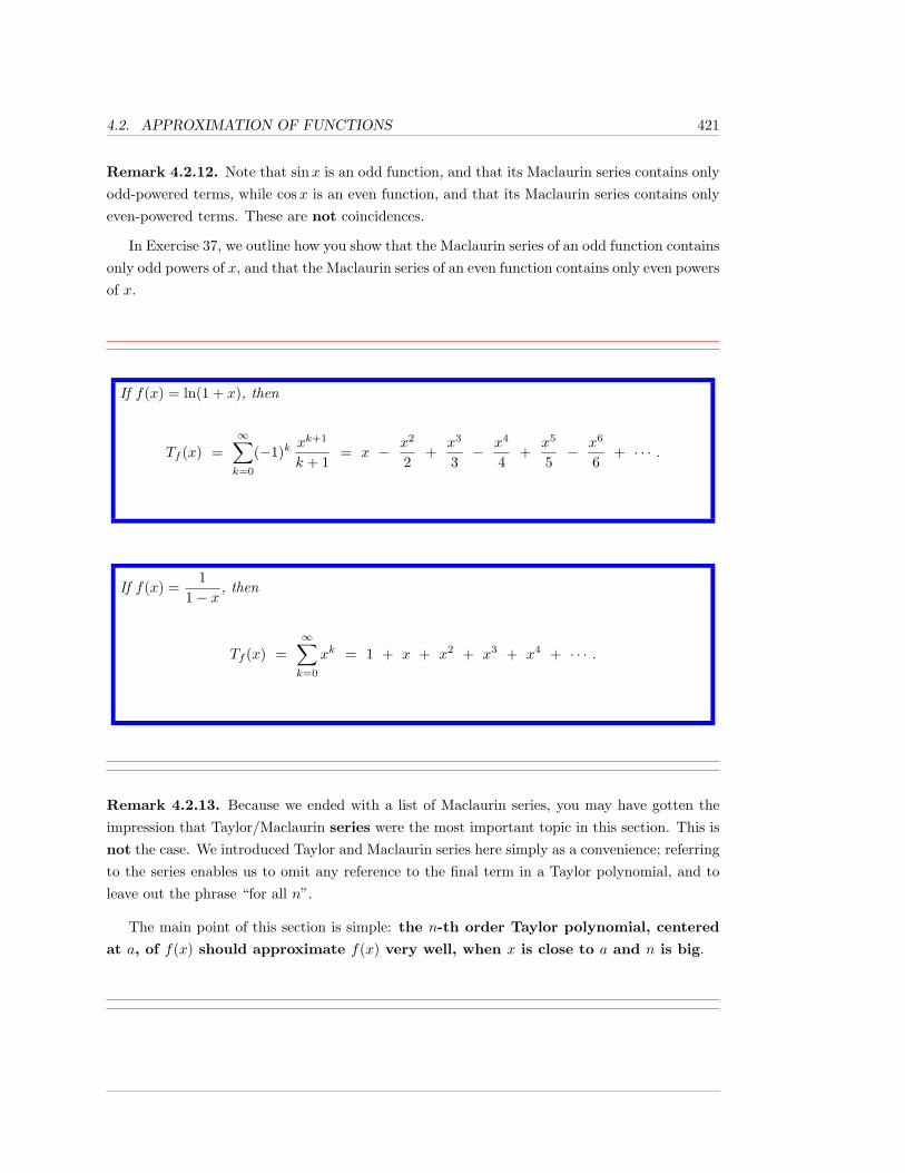
4.2. APPROXIMATION OF FUNCTIONS 421
Remark 4.2.12. Note that sinx is an odd function, and that its Maclaurin series contains onlyodd-powered terms, while cosx is an even function, and that its Maclaurin series contains onlyeven-powered terms. These are not coincidences.
In Exercise 37, we outline how you show that the Maclaurin series of an odd function containsonly odd powers of x, and that the Maclaurin series of an even function contains only even powersof x.
If f(x) = ln(1 + x), then
Tf (x) =∞∑k=0
(−1)kxk+1
k + 1= x − x2
2+
x3
3− x4
4+
x5
5− x6
6+ · · · .
If f(x) =1
1− x, then
Tf (x) =∞∑k=0
xk = 1 + x + x2 + x3 + x4 + · · · .
Remark 4.2.13. Because we ended with a list of Maclaurin series, you may have gotten theimpression that Taylor/Maclaurin series were the most important topic in this section. This isnot the case. We introduced Taylor and Maclaurin series here simply as a convenience; referringto the series enables us to omit any reference to the final term in a Taylor polynomial, and toleave out the phrase “for all n”.
The main point of this section is simple: the n-th order Taylor polynomial, centered
at a, of f(x) should approximate f(x) very well, when x is close to a and n is big.
422 CHAPTER 4. POLYNOMIALS AND POWER SERIES
4.2.1 Exercises
In Exercises 1 through 5, (a) use the five Maclaurin series given in Theorem 4.2.11 to
determine the 1st, 2nd, and 3rd order Maclaurin polynomials of the given function
f , (b) using a calculator, compare the values of f(2) with the values of T 1f (2), T 2
f (2),and T 3
f (2), and explain why your results are not surprising, and (c) using a calculator,
compare the values of f(0.001) with the values of T 1f (0.001), T 2
f (0.001), and T 3f (0.001),
and explain why your results are not surprising.
1. f(x) = ex.
2. f(x) = sinx.
3. f(x) = cosx.
4. f(x) = ln(1 + x).
5. f(x) =1
1− x.
In each of Exercises 6 through 10, (a) determine the 2nd order Taylor polynomial,
centered at the given a, for the given function, (b) using a graphing calculator or
computer graphing program, graph, in a single window, the original function and
T 2f (x; a), for values of x “close” to a.
6. p(x) = (x− 1)3 + (x− 1)2 + (x− 1), a = 0.
7. g(x) = sinhx, a = 0.
8. h(x) = coshx, a = 0.
9. f(x) = e−x, a = 1.
10. r(x) = (1 + x)4, a = 3.
In each of Exercises 11 through 13, find the 3rd order Taylor polynomial, T 3f (x; a),
for the given f and the given a.
11. f(x) = 3√x, a = 1.
12. f(x) =√
1 + x2, a = 0.
13. f(x) = ln(x2), a = 1.
4.2. APPROXIMATION OF FUNCTIONS 423
In Exercises 14 through 18, (a) calculate the specified Tnf (x; a) and (b) the error
between the Taylor approximation and the value given by your calculator.
14. f(x) = sinx.
a. T 3f
(4.7;
3π2
)b.∣∣∣∣sin(4.7)− T 3
f
(4.7;
3π2
)∣∣∣∣15. g(x) = sinhx.
a. T 3g (0.1; 0)
b. | sinh(0.1)− T 3g (0.1; 0)|
16. h(x) = lnx.
a. T 2h (0.9; 1)
b. | ln(0.9)− T 2h (0.9; 1)|
17. v(x) = secx.
a. T 2v (−0.1; 0)
b. | sec(−0.1)− T 2v (−0.1; 0)|
18. w(x) = cosx.
a. T 2w
(1.6;
π
2
)b.∣∣∣cos(1.6)− T 2
w
(1.6;
π
2
)∣∣∣19. What power of x do you expect to approximate sinx well, when x is near 0? That is, if
you want to approximate sinx by a function xn, for x values close to 0, what should n be?
20. What power of x do you expect to approximate 6(x− sinx) well, when x is near 0? Thatis, if you want to approximate 6(x− sinx) by a function xn, for x values close to 0, whatshould n be?
21. If you want to approximate 1− cosx well, by a function of the form cxn, when x is closeto 0, what should you pick for the constant c and the positive integer n?
22. Using a graphing calculator or graphing software, graph f(x) = 1− cosx and g(x) = cxn,using your c and n values from the previous exercise. Graph the functions in the samewindow, with −1 ≤ x ≤ 1 and −0.5 ≤ y ≤ 0.5.
424 CHAPTER 4. POLYNOMIALS AND POWER SERIES
In each of Exercises 23 through 33, determine the Taylor series for the given func-
tion, centered at the given a. Give the Taylor series using summation notation, or
by giving the first 5 non-zero terms, followed by dots.
23. s(x) = e3x, a = −1.
24. u(t) = sin t+ cos t, a = π/2.
25. k(t) = cos(2t), a = π/4.
26. s(t) = 5t, a = 0.
27. k(x) = cosh(2x), a = 0.
28. r(t) = sinh(2t), a = 0.
29. f(t) = ln(1 + 3t), a = 3.
30. m(x) = x, a = 1.
31. n(x) = x2, a = −1.
32. j(x) = lnx, a = 1.
33. s(x) =1
1 + x, a = 1.
34. Describe in a paragraph or two the idea behind why the Taylor polynomials of f , centeredat a, “should” approximate f(x) well for values of x close to a.
35. What is Tnf (x; a) − T (n−1)f (x; a)? Assume f is infinitely differentiable in a neighborhood
of x = a.
36. The approximation sinx ≈ x, when x is close 0, is used often in physics and engineering.Where does this come from?
If you wanted a better approximation of sinx, when x is close to 0, and were willing touse a polynomial with two non-zero terms (instead of one), what polynomial would youuse? Why?
37. In this exercise, we give the steps which show that the Maclaurin series of an even or oddfunction contain only even or, respectively, odd powers of x.
a. Suppose that f is an odd function, which is defined at 0. Show that f(0) = 0.
b. Show that the derivative of an even function is odd, and that the derivative of an oddfunction is even. Conclude that, for infinitely differentiable functions, even-numberedderivatives of odd functions are odd, and odd-numbered derivatives of even functionsare odd.

4.2. APPROXIMATION OF FUNCTIONS 425
c. Show that, if f is infinitely differentiable and defined at 0, then the only (possible)non-zero terms in the Maclaurin series of f are the even-powered terms if f is even,and the odd-powered terms if f is odd.
38. Derive the Maclaurin series for cosx given in Theorem 4.2.11.
39. Derive the Maclaurin series for ln(1 + x) given in Theorem 4.2.11.
40. Derive the Maclaurin series for 1/(1− x) given in Theorem 4.2.11.
426 CHAPTER 4. POLYNOMIALS AND POWER SERIES
4.3 Error in Approximation by Polynomials
In the previous section, we introduced Taylor polynomials, centered at a, of a function f(x).We tried to convince you, on an intuitive level, that the n-th order Taylor polynomial should
approximate the original function well for values of x near the center when n is large, becausewe forced n derivatives of f and the Taylor polynomial to match at a. In this section, we willactually give a result on the error involved, and show how to apply it.
As in Section 4.1, we wish to give names and notations for the remainder and error whenapproximating a function by its Taylor polynomials.
Definition 4.3.1. Suppose that f is n times differentiable at a.Then, we let
Rnf (x; a) = f(x) − Tnf (x; a)
and refer to it as the n-th order Taylor remainder for f , centered at a.
We let Enf (x; a) = |Rnf (x; a)|, and refer to it as the n-th order Taylor error for f ,centered at a.
If a = 0, we naturally refer to these as the n-th order Maclaurin remainder andMaclaurin error for f .
Remark 4.3.2. As Tnf (a; a) = f(a) for all n, the n-th order Taylor remainder and error areboth zero at x = a, i.e., Enf (a; a) = |Rnf (a; a)| = 0.
We now state and prove the one result that we shall use to establish upper bounds on theerror in approximating a function by its Taylor polynomials: the Taylor-Lagrange Theorem.The theorem is a generalization of the Mean Value Theorem for derivatives. Various forms ofthis result are known simply as Taylor’s Theorem. The result that we give is actually Taylor’sTheorem with Lagrange’s form of the remainder, and so we refer to the theorem as the Taylor-Lagrange Theorem.
4.3. ERROR IN APPROXIMATION 427
The condition in the Taylor-Lagrange Theorem that x 6= a is present because the theoremrefers to a number c that’s in the open interval between x and a. This does not mean that wedon’t know what happens when x = a; remember: when x = a, we have already seen that all ofthe Taylor remainders are 0.
Theorem 4.3.3. (Taylor-Lagrange Theorem) Suppose that n is a non-negative integer,and that the (n+ 1)-st derivative of f exists on an open interval I around a point a.
Then, for all x 6= a in I, there exists a c in the open interval between x and a (i.e., in(x, a) if x < a, or in (a, x) if a < x) such that
Rnf (x; a) =f (n+1)(c)(n+ 1)!
(x− a)n+1.
In particular, for all x in I (even if x = a), there exists c in the closed interval betweenx and a such that
Rnf (x; a) =f (n+1)(c)(n+ 1)!
(x− a)n+1.
Proof. This proof is technical. However, as this result is the entire point of this section, we willgive the proof here, rather than relegating it to an appendix.
Assume that x 6= a. Define the function g(t), with domain I, by
g(t) = f(x)−Rnf (x; a)(x− t)n+1
(x− a)n+1−
n∑k=0
f (k)(t)k!
(x− t)k.
Since f is (n + 1)-differentiable on I, g is differentiable on I, and so is certainly continuous onthe closed interval between x and a. One easily sees that g(x) = g(a) = 0. By Rolle’s Theorem(see [2]), there exists c in the open interval between x and a such that g′(c) = 0.
We claim that this shows that Rnf (x; a) =f (n+1)(c)(n+ 1)!
(x − a)n+1, as desired, but we need to
calculate g′(t) in order to see this.
We find, using the Product Rule inside the summation,
g′(t) =
428 CHAPTER 4. POLYNOMIALS AND POWER SERIES
−Rnf (x; a)(n+ 1)(x− t)n(−1)
(x− a)n+1−
n∑k=0
1k!·[f (k+1)(t)(x− t)k + f (k)(t)k(x− t)k−1(−1)
]=
(n+ 1)Rnf (x; a)(x− t)n
(x− a)n+1−
n∑k=0
f (k+1)(t)k!
(x− t)k +n∑k=1
f (k)(t)(k − 1)!
(x− t)k−1.
Let j = k − 1, so that k = j + 1, and use j to re-index the last summation above. We obtain
g′(t) = (n+ 1)Rnf (x; a)(x− t)n
(x− a)n+1−
n∑k=0
f (k+1)(t)k!
(x− t)k +n−1∑j=1
f (j+1)(t)j!
(x− t)j .
Now, in these two summations above, one with a plus sign, one with a minus sign, all of theterms cancel out, except for one: −f (n+1)(t)(x− t)n/(n!).
Therefore, we find that
g′(t) =(n+ 1)(x− t)n
(x− a)n+1·[Rnf (x; a)− f (n+1)(t)
(n+ 1)!(x− a)n+1
].
Since g′(c) = 0 and c is in the open interval between x and a, we know that x− c 6= 0 and so,we conclude that
Rnf (x; a)− f (n+1)(c)(n+ 1)!
(x− a)n+1 = 0,
which is what we needed to show.
Remark 4.3.4. It shouldn’t be too difficult to remember the conclusion of the Taylor-LagrangeTheorem; the n-th remainder
Rnf (x; a) =f (n+1)(c)(n+ 1)!
(x− a)n+1
looks exactly like the (n+ 1)-st order term in the Taylor series for f , except that there is thisunknown c stuck into the (n+ 1)-st derivative instead of the center a.
As we shall see, to use this form of the remainder, we always need to determine an upperbound on the absolute value of f (n+1)(c), an upper bound that does not contain a reference tothe mysterious c.
4.3. ERROR IN APPROXIMATION 429
You should note that the value of c can and, probably, will change when n changes and, forthis reason, we could denote c by the more careful notation cn. However, as our goal is alwaysto place an upper bound on f (n+1)(c) which doesn’t have the c in it, there is no practical needto write cn in place of c.
Example 4.3.5. In Example 4.2.5, we looked at Maclaurin polynomials for f(x) = ex. We sawthat T 1
f (0.1) = 1.1 and T 3f (0.1) = 1.1051666, and we decided to trust our calculators, which told
us that e0.1 “ = ” 1.10517091808.
What if we don’t want to rely on our calculator? Can we use the Taylor-Lagrange The-orem to obtain upper bounds on the error if we approximate e0.1 by the 1st and 3rd orderMaclaurin polynomials? We could also ask what order Maclaurin polynomial we would need touse, according to the Taylor-Lagrange Theorem, to obtain the 11 decimal place accuracy of ourcalculators.
Certainly ex is infinitely differentiable on the entire real line, so the hypothesis of the Taylor-Lagrange Theorem about being differentiable (n+1) times on an open interval I around a holdsfor all a and for I = (−∞,∞).
Therefore, the error in approximating e0.1 by the n-th order Maclaurin polynomial Tnf (x) isgiven by
Enf (0.1) =∣∣Rnf (0.1)
∣∣ =∣∣∣∣f (n+1)(c)
(n+ 1)!(0.1)n+1
∣∣∣∣ =(0.1)n+1
(n+ 1)!
∣∣f (n+1)(c)∣∣,
for some c in the closed interval [0, 0.1]. Of course, all of the derivatives of ex are just ex. Now,f (n+1)(c) = ec, which is always positive, and so we have
Enf (0.1) =(0.1)n+1 ec
(n+ 1)!,
for some c in the closed interval [0, 0.1]. But what do we do with this ec factor, when we don’tknow what c is?
The quick answer: we say that the ec factor is less than or equal to something which has noc in it. This means that we won’t know the exact error, but will be able to say that the erroris no more than a certain amount, which is what we really need in most applications.
430 CHAPTER 4. POLYNOMIALS AND POWER SERIES
Since c is in the closed interval [0, 0.1], and f(x) = ex is an increasing function (since it’sderivative ex is always positive), regardless of what c is, we know that ec ≤ e0.1. Thus, we know
Enf (0.1) ≤ (0.1)n+1 e0.1
(n+ 1)!.
At this point, your reaction may be something like “But...but...our whole goal was to find a goodapproximation of e0.1, and now our upper bound on the error contains e0.1. Isn’t this circular?”
No – because we can now use some fairly awful upper bound, that doesn’t have to bevery accurate, for e0.1, and then conclude how big n needs to be so that our gross upper boundguarantees that Enf (0.1) is really small. So, no, our argument will not be “circular”, but will seemclose to it; we will use a gross upper bound for e0.1 to obtain arbitrarily good approximationsof e0.1. Cool, huh?
How does this work? We will use that e0.1 ≤ 2. Why is this true? Because certainly e ≤ 210!So, now we have that
Enf (0.1) ≤ (0.1)n+1 e0.1
(n+ 1)!≤ (0.1)n+1 · 2
(n+ 1)!. (4.5)
Note that our upper bound on the error decreases as n increases, so that using higher-orderMaclaurin polynomials gives a smaller upper bound on the error in the approximation. This iswhat we want and expect.
Now we’re ready to answer the questions that we asked at the beginning of this section.
When n = 1, Formula 4.5 tells us that
E1f (0.1) ≤ (0.1)1+1 · 2
(1 + 1)!= 0.01.
In fact, what we really found before, trusting our calculators, is that
E1f (0.1) =
∣∣e0.1 − T 1f (0.1)
∣∣ “ = ” |1.10517091808− 1.1| = 0.00517091808.
Thus, the actual error is roughly half of what we produced for an upper bound, but what’simportant is that the error is less than or equal to our upper bound of 0.01, as it had tobe. It is not terribly surprising that our upper bound is “far” from the actual error; we used arough upper bound for ec, and then we used that e ≤ 210.
The point is that it is more important to end up with a manageable upper bound
4.3. ERROR IN APPROXIMATION 431
than to end up with a more accurate, but unmanageable, upper bound.
When n = 3, Formula 4.5 tells us that
E3f (0.1) ≤ (0.1)3+1 · 2
(3 + 1)!=
0.000224
= 0.000008333.
Of course, once again trusting our calculators, you should check that the “actual” error is roughlyhalf of this.
Finally, if we were the ones setting up your calculator with a Maclaurin polynomial to ap-proximate e0.1 to within 11 decimal places, what order Maclaurin polynomial would Formula 4.5tell us is good enough? That is, what’s the smallest n such that our upper bound on the errorEnf (0.1) is less than 5(10)−12, so that the digit in the 12th decimal place is less than 5, androunding will give the “correct” answer?
We want the smallest n such that
(0.1)n+1 · 2(n+ 1)!
≤ 5(10)−12.
The bad news is that there are no algebraic rules that will let you solve for such an n. Thegood news is that if n is 11, (0.1)n+1 = (10)−12 and 2/(12!) is much less than 1, so n = 11 isdefinitely big enough, but how do we find the smallest such n? The easy way – just check theother n values less than 11, either by hand or with a calculator. You can start at n = 0 and goup, or start at n = 11 and go down.
We leave it as an exercise for you to show that the answer is n = 7. Hence, the 7th orderMaclaurin polynomial for ex can be used to approximate e0.1 to 11 decimal place accuracy.
It is worth noting that n = 7 is good enough, and it’s the smallest n that makes our upperbound less than 5(10)−12, but, since our upper bound is not, itself, the actual error (probably),it is possible that some more difficult, or different, argument would tell us a smaller n so thatEnf (0.1) is less than 5(10)−12. But we’re happy with knowing that n = 7 forces our relativelyeasy upper bound on the error to be less than 5(10)−12, which, in turn, forces the error itself tobe less than 5(10)−12.
Example 4.3.6. Suppose that x is within±0.2 of π/2. If we use the 4th order Taylor polynomial
432 CHAPTER 4. POLYNOMIALS AND POWER SERIES
of f(x) = sinx, centered at π/2, to approximate sinx, how accurate can we be certain that ourapproximation is?
Solution:
As in the last example, we will find a gross upper bound on the error Enf (x;π/2), and thensee how big this upper bound is. We shall first look at the situation for general n, and thendiscuss what happens when n = 4; there is something special which happens in this example,something which did not occur in the previous example.
The Taylor-Lagrange Theorem tells us that the error Enf (x) in approximating sinx byTnf (x;π/2) is given by
Enf (x;π/2) =∣∣∣Rnf (x;
π
2
)∣∣∣ =∣∣∣∣f (n+1)(c)
(n+ 1)!
(x− π
2
)n+1∣∣∣∣ =
∣∣∣x− π
2
∣∣∣n+1
(n+ 1)!·∣∣f (n+1)(c)
∣∣,where c is between x and π/2, and so is also within ±0.2 of π/2.
We were told that x is within ±0.2 of π/2; this means precisely that |x− π/2| ≤ 0.2. Thus,we know that
Enf (x;π/2) ≤ (0.2)n+1
(n+ 1)!·∣∣f (n+1)(c)
∣∣.As in all such problems, we need to find an upper bound on
∣∣f (n+1)(c)∣∣. How do we do this?
The manner by which you produce such an upper bound varies from function to function, but,this time, is particularly easy.
All of the derivatives of sine are equal to plus or minus sine or cosine, i.e., f (n+1)(c) is oneof ± sin c or ± cos c. As the values of sine and cosine are always between −1 and 1, the absolutevalues of plus or minus sine or cosine are all less than or equal to 1. Hence,
∣∣f (n+1)(c)∣∣ ≤ 1, and
Enf (x;π/2) ≤ (0.2)n+1
(n+ 1)!·∣∣f (n+1)(c)
∣∣ ≤ (0.2)n+1
(n+ 1)!· 1.
When n = 4, we find
E4f (x;π/2) ≤ (0.2)4+1
(4 + 1)!= 0.000002666.
4.3. ERROR IN APPROXIMATION 433
Recall that we found the Taylor series for sinx, centered at π/2, in Example 4.2.8; we found
T∞f
(x;π
2
)= 1− 1
2!
(x− π
2
)2
+14!
(x− π
2
)4
− 16!
(x− π
2
)6
+ · · · . (4.6)
It’s 4th order partial sum, the 4th order Taylor polynomial is
T 4f
(x;π
2
)= 1− 1
2!
(x− π
2
)2
+14!
(x− π
2
)4
,
which has only three non-zero terms. It’s pretty amazing that these three non-zero polynomialterms let us approximate sinx to within ±0.000002666, provided that we know that x is within±0.2 of π/2.
However, by being slightly tricky, we can actually conclude that the error is substantiallysmaller. Since all of the odd-powered terms are missing/zero in Formula 4.6, T 4
f (x;π/2) =T 5f (x;π/2), which implies that E4
f (x;π/2) = E5f (x;π/2). Now, our upper bound on Enf (x;π/2)
says that
E4f (x;π/2) = E5
f (x;π/2) ≤ (0.2)5+1
(5 + 1)!= 0.0000000888.
So, T 4f (x;π/2) yields a stunningly accurate approximation for x in the given range. For
instance, when x = 0.1 + π/2, a calculator tells us that
sin(
0.1 +π
2
)“ = ” 0.995004165278,
while
T 4f
(0.1 +
π
2;π
2
)= 1− 1
2!(0.1)2 +
14!
(0.1)4 = 0.995004166666.
Example 4.3.7. Let f(x) = cos(3x).
a. Suppose that |x| ≤ 0.1. Find a “reasonable” upper-bound on the error in approximatingf(x) by T 3
f (x; 0).
b. Suppose that |x| ≤ 0.1. By using “reasonable” bounds, find the smallest n such that youcan prove that the error in approximating f(x) by Tnf (x; 0) is less than or equal to 0.0001.
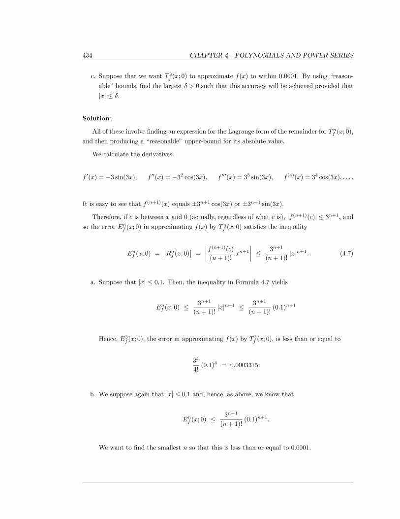
434 CHAPTER 4. POLYNOMIALS AND POWER SERIES
c. Suppose that we want T 3f (x; 0) to approximate f(x) to within 0.0001. By using “reason-
able” bounds, find the largest δ > 0 such that this accuracy will be achieved provided that|x| ≤ δ.
Solution:
All of these involve finding an expression for the Lagrange form of the remainder for Tnf (x; 0),and then producing a “reasonable” upper-bound for its absolute value.
We calculate the derivatives:
f ′(x) = −3 sin(3x), f ′′(x) = −32 cos(3x), f ′′′(x) = 33 sin(3x), f (4)(x) = 34 cos(3x), . . . .
It is easy to see that f (n+1)(x) equals ±3n+1 cos(3x) or ±3n+1 sin(3x).
Therefore, if c is between x and 0 (actually, regardless of what c is), |f (n+1)(c)| ≤ 3n+1, andso the error Enf (x; 0) in approximating f(x) by Tnf (x; 0) satisfies the inequality
Enf (x; 0) =∣∣Rnf (x; 0)
∣∣ =∣∣∣∣f (n+1)(c)
(n+ 1)!xn+1
∣∣∣∣ ≤ 3n+1
(n+ 1)!|x|n+1. (4.7)
a. Suppose that |x| ≤ 0.1. Then, the inequality in Formula 4.7 yields
Enf (x; 0) ≤ 3n+1
(n+ 1)!|x|n+1 ≤ 3n+1
(n+ 1)!(0.1)n+1
Hence, E3f (x; 0), the error in approximating f(x) by T 3
f (x; 0), is less than or equal to
34
4!(0.1)4 = 0.0003375.
b. We suppose again that |x| ≤ 0.1 and, hence, as above, we know that
Enf (x; 0) ≤ 3n+1
(n+ 1)!(0.1)n+1.
We want to find the smallest n so that this is less than or equal to 0.0001.
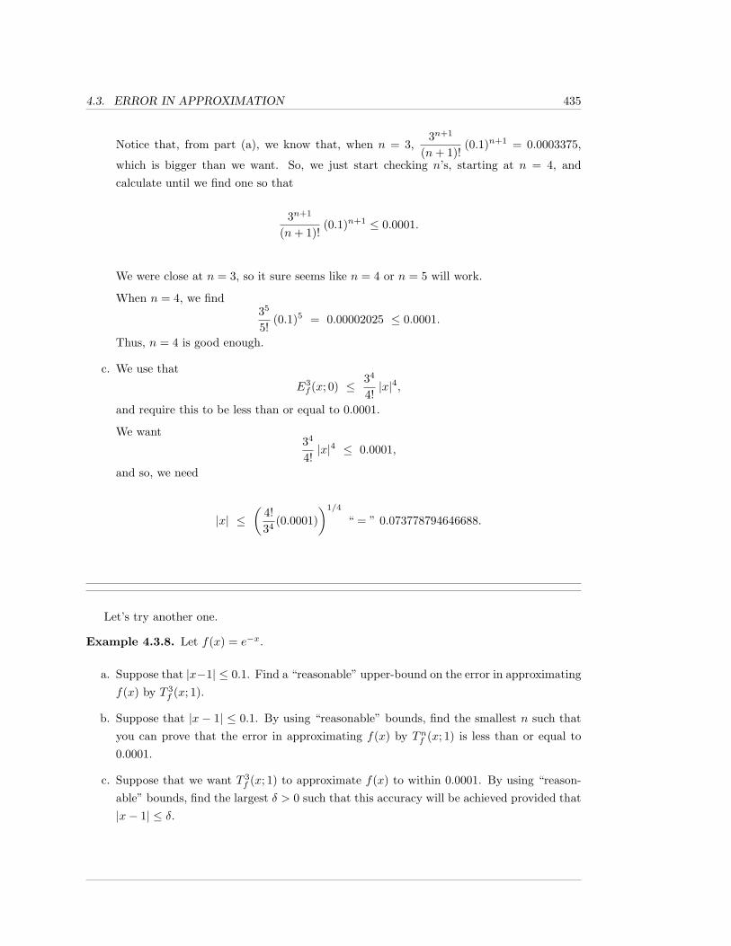
4.3. ERROR IN APPROXIMATION 435
Notice that, from part (a), we know that, when n = 3,3n+1
(n+ 1)!(0.1)n+1 = 0.0003375,
which is bigger than we want. So, we just start checking n’s, starting at n = 4, andcalculate until we find one so that
3n+1
(n+ 1)!(0.1)n+1 ≤ 0.0001.
We were close at n = 3, so it sure seems like n = 4 or n = 5 will work.
When n = 4, we find35
5!(0.1)5 = 0.00002025 ≤ 0.0001.
Thus, n = 4 is good enough.
c. We use thatE3f (x; 0) ≤ 34
4!|x|4,
and require this to be less than or equal to 0.0001.
We want34
4!|x|4 ≤ 0.0001,
and so, we need
|x| ≤(
4!34
(0.0001))1/4
“ = ” 0.073778794646688.
Let’s try another one.
Example 4.3.8. Let f(x) = e−x.
a. Suppose that |x−1| ≤ 0.1. Find a “reasonable” upper-bound on the error in approximatingf(x) by T 3
f (x; 1).
b. Suppose that |x − 1| ≤ 0.1. By using “reasonable” bounds, find the smallest n such thatyou can prove that the error in approximating f(x) by Tnf (x; 1) is less than or equal to0.0001.
c. Suppose that we want T 3f (x; 1) to approximate f(x) to within 0.0001. By using “reason-
able” bounds, find the largest δ > 0 such that this accuracy will be achieved provided that|x− 1| ≤ δ.
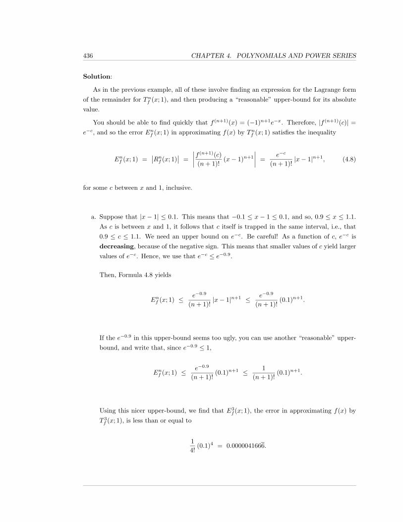
436 CHAPTER 4. POLYNOMIALS AND POWER SERIES
Solution:
As in the previous example, all of these involve finding an expression for the Lagrange formof the remainder for Tnf (x; 1), and then producing a “reasonable” upper-bound for its absolutevalue.
You should be able to find quickly that f (n+1)(x) = (−1)n+1e−x. Therefore, |f (n+1)(c)| =e−c, and so the error Enf (x; 1) in approximating f(x) by Tnf (x; 1) satisfies the inequality
Enf (x; 1) =∣∣Rnf (x; 1)
∣∣ =∣∣∣∣f (n+1)(c)
(n+ 1)!(x− 1)n+1
∣∣∣∣ =e−c
(n+ 1)!|x− 1|n+1, (4.8)
for some c between x and 1, inclusive.
a. Suppose that |x − 1| ≤ 0.1. This means that −0.1 ≤ x − 1 ≤ 0.1, and so, 0.9 ≤ x ≤ 1.1.As c is between x and 1, it follows that c itself is trapped in the same interval, i.e., that0.9 ≤ c ≤ 1.1. We need an upper bound on e−c. Be careful! As a function of c, e−c isdecreasing, because of the negative sign. This means that smaller values of c yield largervalues of e−c. Hence, we use that e−c ≤ e−0.9.
Then, Formula 4.8 yields
Enf (x; 1) ≤ e−0.9
(n+ 1)!|x− 1|n+1 ≤ e−0.9
(n+ 1)!(0.1)n+1.
If the e−0.9 in this upper-bound seems too ugly, you can use another “reasonable” upper-bound, and write that, since e−0.9 ≤ 1,
Enf (x; 1) ≤ e−0.9
(n+ 1)!(0.1)n+1 ≤ 1
(n+ 1)!(0.1)n+1.
Using this nicer upper-bound, we find that E3f (x; 1), the error in approximating f(x) by
T 3f (x; 1), is less than or equal to
14!
(0.1)4 = 0.0000041666.
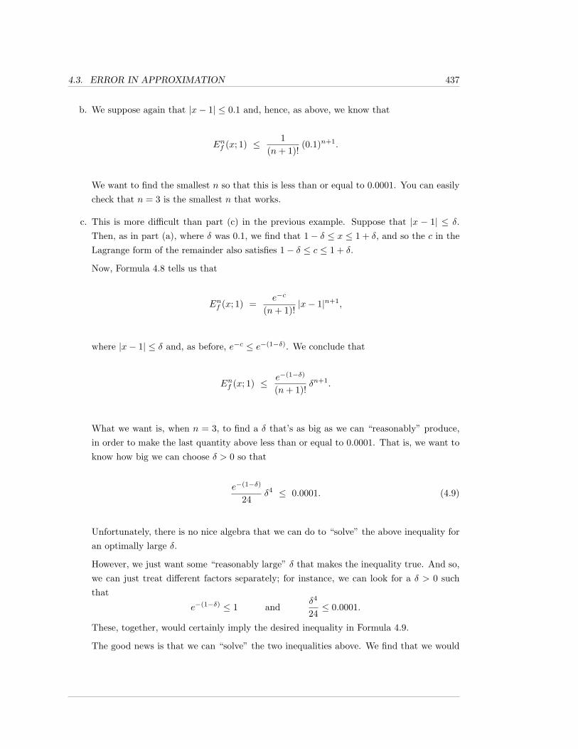
4.3. ERROR IN APPROXIMATION 437
b. We suppose again that |x− 1| ≤ 0.1 and, hence, as above, we know that
Enf (x; 1) ≤ 1(n+ 1)!
(0.1)n+1.
We want to find the smallest n so that this is less than or equal to 0.0001. You can easilycheck that n = 3 is the smallest n that works.
c. This is more difficult than part (c) in the previous example. Suppose that |x − 1| ≤ δ.Then, as in part (a), where δ was 0.1, we find that 1− δ ≤ x ≤ 1 + δ, and so the c in theLagrange form of the remainder also satisfies 1− δ ≤ c ≤ 1 + δ.
Now, Formula 4.8 tells us that
Enf (x; 1) =e−c
(n+ 1)!|x− 1|n+1,
where |x− 1| ≤ δ and, as before, e−c ≤ e−(1−δ). We conclude that
Enf (x; 1) ≤ e−(1−δ)
(n+ 1)!δn+1.
What we want is, when n = 3, to find a δ that’s as big as we can “reasonably” produce,in order to make the last quantity above less than or equal to 0.0001. That is, we want toknow how big we can choose δ > 0 so that
e−(1−δ)
24δ4 ≤ 0.0001. (4.9)
Unfortunately, there is no nice algebra that we can do to “solve” the above inequality foran optimally large δ.
However, we just want some “reasonably large” δ that makes the inequality true. And so,we can just treat different factors separately; for instance, we can look for a δ > 0 suchthat
e−(1−δ) ≤ 1 andδ4
24≤ 0.0001.
These, together, would certainly imply the desired inequality in Formula 4.9.
The good news is that we can “solve” the two inequalities above. We find that we would
438 CHAPTER 4. POLYNOMIALS AND POWER SERIES
like a δ > 0 such that
δ ≤ 1 and δ ≤ 4√
(24)(0.0001) = 0.1 4√
24 ≤ 0.222.
Of course, requiring δ ≤ 0.1 4√
24 already implies that δ ≤ 1. Thus, choosing δ = 0.1 4√
24would be “reasonable”.
4.3.1 Exercises
1. Let f(x) = sin(x
2
).
a. Suppose that |x| ≤ 0.1. Find a “reasonable” upper-bound on the error in approxi-mating f(x) by T 3
f (x; 0).
b. Suppose that |x| ≤ 0.1. By using “reasonable” bounds, find the smallest n such thatyou can prove that the error in approximating f(x) by Tnf (x; 0) is less than or equalto 0.0001.
c. Suppose that we want T 3f (x; 0) to approximate f(x) to within 0.0001. By using
“reasonable” bounds, find the largest δ > 0 such that this accuracy will be achievedprovided that |x| ≤ δ.
2. Let f(x) = e3x.
a. Suppose that |x| ≤ 0.1. Find a “reasonable” upper-bound on the error in approxi-mating f(x) by T 3
f (x; 0).
b. Suppose that |x| ≤ 0.1. By using “reasonable” bounds, find the smallest n such thatyou can prove that the error in approximating f(x) by Tnf (x; 0) is less than or equalto 0.0001.
c. Suppose that we want T 3f (x; 0) to approximate f(x) to within 0.0001. By using
“reasonable” bounds, find the largest δ > 0 such that this accuracy will be achievedprovided that |x| ≤ δ.
3. Let f(x) = sin(5x).
a. Suppose that |x−1| ≤ 0.1. Find a “reasonable” upper-bound on the error in approx-imating f(x) by T 3
f (x; 1).
4.3. ERROR IN APPROXIMATION 439
b. Suppose that |x − 1| ≤ 0.1. By using “reasonable” bounds, find the smallest n suchthat you can prove that the error in approximating f(x) by Tnf (x; 1) is less than orequal to 0.0001.
c. Suppose that we want T 3f (x; 1) to approximate f(x) to within 0.0001. By using
“reasonable” bounds, find the largest δ > 0 such that this accuracy will be achievedprovided that |x− 1| ≤ δ.
4. Let f(x) = e7x.
a. Suppose that |x−1| ≤ 0.1. Find a “reasonable” upper-bound on the error in approx-imating f(x) by T 3
f (x; 1).
b. Suppose that |x − 1| ≤ 0.1. By using “reasonable” bounds, find the smallest n suchthat you can prove that the error in approximating f(x) by Tnf (x; 1) is less than orequal to 0.0001.
c. Suppose that we want T 3f (x; 1) to approximate f(x) to within 0.0001. By using
“reasonable” bounds, find the largest δ > 0 such that this accuracy will be achievedprovided that |x− 1| ≤ δ.
5. Let f(x) = lnx.
a. Suppose that |x−1| ≤ 0.1. Find a “reasonable” upper-bound on the error in approx-imating f(x) by T 3
f (x; 1).
b. Suppose that |x − 1| ≤ 0.1. By using “reasonable” bounds, find the smallest n suchthat you can prove that the error in approximating f(x) by Tnf (x; 1) is less than orequal to 0.0001.
c. Suppose that we want T 3f (x; 1) to approximate f(x) to within 0.0001. By using
“reasonable” bounds, find the largest δ > 0 such that this accuracy will be achievedprovided that |x− 1| ≤ δ.
6. Let f(x) = cos(x
3
).
a. Suppose that |x−1| ≤ 0.1. Find a “reasonable” upper-bound on the error in approx-imating f(x) by T 3
f (x; 1).
b. Suppose that |x − 1| ≤ 0.1. By using “reasonable” bounds, find the smallest n suchthat you can prove that the error in approximating f(x) by Tnf (x; 1) is less than orequal to 0.0001.
c. Suppose that we want T 3f (x; 1) to approximate f(x) to within 0.0001. By using
“reasonable” bounds, find the largest δ > 0 such that this accuracy will be achievedprovided that |x− 1| ≤ δ.
440 CHAPTER 4. POLYNOMIALS AND POWER SERIES
7. Let f(x) = x5.
a. Suppose that |x+ 1| ≤ 0.1. Find a “reasonable” upper-bound on the error in approx-imating f(x) by T 3
f (x;−1).
b. Suppose that |x + 1| ≤ 0.1. By using “reasonable” bounds, find the smallest n suchthat you can prove that the error in approximating f(x) by Tnf (x;−1) is less than orequal to 0.0001.
c. Suppose that we want T 3f (x;−1) to approximate f(x) to within 0.0001. By using
“reasonable” bounds, find the largest δ > 0 such that this accuracy will be achievedprovided that |x| ≤ δ.
8. Let f(x) = x7.
a. Suppose that |x+ 1| ≤ 0.1. Find a “reasonable” upper-bound on the error in approx-imating f(x) by T 3
f (x;−1).
b. Suppose that |x + 1| ≤ 0.1. By using “reasonable” bounds, find the smallest n suchthat you can prove that the error in approximating f(x) by Tnf (x;−1) is less than orequal to 0.0001.
c. Suppose that we want T 3f (x;−1) to approximate f(x) to within 0.0001. By using
“reasonable” bounds, find the largest δ > 0 such that this accuracy will be achievedprovided that |x| ≤ δ.
9. Let f(x) = x− sinx.
a. What is T 5f (x; 0)?
b. Suppose that |x| ≤ 1. Find a “reasonable” upper-bound on the error in approximatingf(x) by T 5
f (x; 0).
10. Let f(x) = 1− cosx.
a. What is T 5f (x; 0)?
b. Suppose that |x| ≤ 1. Find a “reasonable” upper-bound on the error in approximatingf(x) by T 5
f (x; 0).
Recall that the Extreme Value Theorem (see [2]) tells us that a continuous function
defined on a closed interval is bounded. Combining this with the Taylor-Lagrange
Theorem, it follows that, if f (n+1) is continuous on the closed interval [a − δ, a + δ],
then there exists a constant M such that |Rnf (x; a)| ≤ M
(n+ 1)!|x− a|n+1.
Use this result in Exercises 11 through 16 to find an upper bound on Enf (x; 0) =|Rnf (x; 0)| where x is within ±δ of zero; this amounts to finding the maximum of
|f (n+1)(c)| for c in the interval [−δ, δ].
4.3. ERROR IN APPROXIMATION 441
11. f(x) = ex, δ = 1.
12. f(x) = cosx, δ = 0.3.
13. f(x) = sinx, δ = 0.3.
14. f(x) = ln(1 + x), δ = 0.1.
15. f(x) = coshx, δ = 1.
16. f(x) = sinhx, δ = 1.
17. If f is an infinitely differentiable function, what is Enf (a; a)?
18. Explain why the Mean Value Theorem is a special case of the Taylor-Lagrange Theorem.
19. Prove that if f (k+1) is continuous at x = a, then limx→a
∣∣∣∣∣Rkf (x; a)(x− a)k
∣∣∣∣∣ = 0.
20. a. Suppose that k ≥ 0, and that f (k+1)(a) exists. Use the actual definition of theremainder (and the derivative), and iterate l’Hopital’s Rule (see [2]) to prove that
limx→a
Rkf (x; a)(x− a)k+1
=1
(k + 1)!f (k+1)(a).
(Hint: To apply l’Hopital’s Rule, you will need to use that the existence of f (k+1)(a)implies that all lower-order derivatives of f exist for all x in an open interval arounda.)
b. Prove a stronger (and harder) result than that in the previous exercise; prove that,
if f (k+1)(a) exists, then limx→a
∣∣∣∣∣Rkf (x; a)(x− a)k
∣∣∣∣∣ = 0.
21. In this exercise, you will reprove the Second Derivative Test (see [2]). Suppose thatf ′(a) = 0 and that f ′′(a) exists.
a. Use the results of the previous exercise to show that limx→af(x)− f(a)
(x− a)2=
12f ′′(a).
b. Suppose that f ′′(a) > 0. Conclude that f attains a local minimum value at x = a.
c. Suppose that f ′′(a) < 0. Conclude that f attains a local maximum value at x = a.
22. Use the approach in the previous problem to prove the following Third Derivative Test.If f (3)(a) exists and is non-zero, f ′(a) = 0, and f ′′(a) = 0, then f attains neither a localmaximum nor a local minimum value at x = a.
442 CHAPTER 4. POLYNOMIALS AND POWER SERIES
23. Prove that, if k is even and f ′(a) = f ′′(a) = ... = f (k−1)(a) = 0, but f (k)(a) 6= 0,then f attains a local minimum (respectively, maximum) value at x = a if f (k)(a) > 0(respectively, f (k)(a) < 0).
24. Prove that, given the same hypotheses as the previous problem except that k is odd, fattains neither a local maximum nor a local minimum value at x = a.
25. Let f(x) = ex. For part (a), use the fact, proved in [2], that e < 3.
a. Show that 0 < |Rkf (1; 0)| < 3(k + 1)!
.
b. Estimate the value of e to within 0.001 of the correct value.
26. In this problem, we will prove that e is irrational. We will do this by contradiction; so,assume that e is rational and is equal to p/q, where p and q are both positive integers. Wewish to derive a contradiction from this assumption. Let f(x) = ex.
a. Use part (b) of the previous problem to argue that q ≥ 2.
b. Show that, since we’re assuming that e = p/q, it follows that
p
q= 1 + 1 +
12!
+ ...+1q!
+Rqf (1; 0),
where 0 < Rqf (1; 0) <3
(q + 1)!by the previous exercise.
c. Multiply both sides of the equation in part (b) by q!. Reach a contradiction byrearranging the resulting equation and arguing that one side is an integer and theother side is not.
In the next exercise, you’ll prove a different version of Taylor’s Theorem; you will
prove Taylor’s Theorem with Integral Remainder.
27. Suppose that f is continuously differentiable. Then, the Fundamental Theorem of Calcu-
lus, Theorem 2.4.10, tells us that∫ x
a
f ′(t) dt = f(x) − f(a). Also, recall the formula for
integration by parts, Theorem 1.1.19, in the context of definite integration :
∫ b
a
h(y)g′(y) dy = h(b)g(b)− h(a)g(a)−∫ b
a
h′(y)g′(y) dy.
4.3. ERROR IN APPROXIMATION 443
a. Apply integration by parts to∫ x
a
f ′(t) dt with h(t) = f ′(t) and g(t) = t−x to obtain
the formulaf(x) = f(a) + f ′(a)(x− a) +
∫ x
a
(x− t)f ′′(t) dt,
provided that f possesses a continuous second derivative.
b. Apply integration by parts a second time to obtain the formula
f(x) = f(a) + f ′(a)(x− a) +12
(x− a)2 +12
∫ x
a
(x− t)2f ′′′(t) dt,
provided that f possesses a continuous third derivative.
c. Argue inductively that
f(x) = f(a)+f ′(a)(x−a)+12f ′′(a)(x−a)2+...+
f (n)(a)n!
(x−a)n+1n!
∫ x
a
(x−t)nf (n+1)(t) dt,
provided that f possesses a continuous (n + 1)-th derivative. Thus, if f possesses acontinuous (n+ 1)-th derivative,
Rnf (x; a) =1n!
∫ x
a
(x− t)nf (n+1)(t) dt.
This is Taylor’s Theorem with Integral Remainder.
28. Suppose that f (n+1) exists and is continuous. Fix an a and an x.
a. Explain why there exists M ≥ 0 such that |f (n+1)(t)| ≤ M for all t in the closedinterval between a and x.
b. Use the M from part (a) and Taylor’s Theorem with Integral Remainder to show
that |Rnf (x; a)| ≤ M
(n+ 1)!|x − a|n+1. Note that we obtained this same bound prior
to Exercise 11, by using Lagrange’s form of the remainder.
444 CHAPTER 4. POLYNOMIALS AND POWER SERIES
4.4 Functions as Power Series
In the previous two sections, we first looked informally at approximating functions by their Tay-lor polynomials, and then we got formal and used the Taylor-Lagrange Theorem to put boundson the error in the Taylor approximations. Along the way, as a convenient notational device,we introduced Taylor series; these are formal algebraic objects, which are like polynomials,centered at a, except they don’t (necessarily) stop. We did not say, in those earlier sections,that Taylor series define functions.
In this section, we will discuss when a Taylor series T∞f (x; a) defines a function which isequal to the original function f(x), for, at least, some values of x close to the center a. It iscommon to say that the original function can be represented by its Taylor series. We will thengive examples/theorems involving familiar functions.
Note that this section deals with when the Taylor series T∞f (x; a) of a given function f
defines a function in its own right, and when the function T∞f (x; a) equals the original functionf . This section can be viewed as an introduction to using power series as functions. Results onfunctions that are initially defined as power series, or manipulations of power series functions,are dealt with in Section 4.5 and Section 4.6.
Suppose that f(x) is infinitely differentiable at a point a. Then, for all n, we have definedthe n-th order Taylor polynomial
Tnf (x; a) =n∑k=0
f (k)(a)k!
(x− a)k.
Of course, the Taylor polynomials also give us Taylor polynomial functions and, in the previoussections, we looked at the error Enf (x; a) in approximating f(x) by using the functions Tnf (x; a).
We also defined the formal algebraic Taylor series:
T∞f (x; a) =∞∑k=0
f (k)(a)k!
(x− a)k =
f(a) + f ′(a)(x− a) +f ′′(a)
2!(x− a)2 +
f ′′′(a)3!
(x− a)3 + · · · ,
4.4. FUNCTIONS AS POWER SERIES 445
which was really just a way of indicating that we weren’t thinking of looking at just one Taylorpolynomial, but rather were interested in looking at what happens as we take arbitrarily high-order Taylor polynomials.
Our question now is: can we somehow think of the infinite sum in the Taylor series
as defining a function, and can we say when such a Taylor series function is equal
to the original function f(x)?
Since this is a Calculus book, limits may/should come to mind; we can define the infiniteTaylor sum to be the limit, as n approaches infinity, of the n-th order partial sums, i.e., of then-th order Taylor polynomials. (Note that, here, the limit uses only integer values for n; thus,it is the limit of a sequence, as defined in [2], and as we shall see again in Definition 4.5.1.)
Of course, we can make this definition; the question is: does such a definition give usanything useful? As we shall see, the answer is “yes”, and so we make a definition.
Definition 4.4.1. Suppose that f is infinitely differentiable at a.Then, the value, at a point x0, of the Taylor series of f , centered at a, is
T∞f (x0; a) = limn→∞
Tnf (x0; a) =
limn→∞
[f(a) + f ′(a)(x0 − a) +
f ′′(a)2!
(x0 − a)2 +f ′′′(a)
3!(x0 − a)3 + · · ·+ f (n)(a)
n!(x0 − a)n
],
provided that this limit exists; in this case, we say that the Taylor series T∞f (x; a) of f ,centered at a, converges at x0.
If the limit fails to exist, we say that T∞f (x; a) diverges at x0.
The Taylor series function of f , centered at a, is the function whose domain is the setof x0 at which T∞f (x; a) converges, and its value at any x0 in its domain is T∞f (x0; a), asdefined above. The codomain is taken to be all real numbers. The notation for this functionis the same as that of the algebraic Taylor series: Tf (x; a) = T∞f (x; a).
Usually, the Taylor series function is referred to simply as the Taylor series, and the contextmakes it clear whether we mean as a formal algebraic object or as a function; this is why thereis not separate notation for the algebraic Taylor series and the Taylor series function.
446 CHAPTER 4. POLYNOMIALS AND POWER SERIES
Since we expect the Taylor polynomials of f to approximate f well, near the center, andfor the approximation to get better as we take higher-order Taylor polynomials, what wehope/expect is that, if a Taylor series converges at some x0, then what it converges to isf(x0), i.e., we expect that f(x0) = T∞f (x0; a). In other words, we expect, as functions ofx, that f(x) = T∞f (x; a), at least for x values near a. Surprisingly, this is not always true (seeExample 4.4.11).
However, something that’s not surprising is the following theorem, which tells us that it’s alla question of whether the remainder approaches 0 or not.
Theorem 4.4.2. Suppose that f is infinitely differentiable at a. Then, for a given x,limn→∞Enf (x; a) = 0 if and only if T∞f (x; a) converges to f(x), i.e., if and only if
f(x) = T∞f (x; a).
Proof. As Enf (x; a) =∣∣Rnf (x; a)
∣∣, the equality limn→∞Enf (x; a) = 0 is equivalent to limn→∞Rnf (x; a) =0, which means precisely that
limn→∞
[f(x)− Tnf (x; a)
]= 0,
i.e.,
f(x) = limn→∞
Tnf (x; a) = T∞f (x; a).
Remark 4.4.3. We should make three comments.
First, we usually omit the explicit assumption in Theorem 4.4.2 that f is infinitely differen-tiable at a; this omission causes no confusion since, when we give a statement involving T∞f (x; a),it is clear that we are, in fact, assuming that the formal algebraic series T∞f (x; a) exists, i.e.,that f is infinitely differentiable at a.
4.4. FUNCTIONS AS POWER SERIES 447
Second, the way in which we usually show that Enf (x; a) → 0 is to find some upper boundUnf (x; a) on Enf (x; a), and then show that Unf (x; a)→ 0 as n→∞. This implies that Enf (x; a)→0, since
0 ≤ Enf (x; a) ≤ Unf (x; a),
and Enf (x; a) gets pinched to 0 as Unf (x; a)→ 0.
Finally, it is, of course, always true that T∞f (x; a) converges to f(x) at the single point x = a,for then all of the (x− a)’s are 0. What’s interesting is not when T∞f (x; a) converges to f(x) atjust x = a, but rather when T∞f (x; a) converges to f(x) for all x near a.
Before we look at some examples, we will state an easy lemma, which is useful, in variousproblems, in showing that limn→∞Enf (x; a) = 0.
Lemma 4.4.4. Suppose that x is a fixed real number.
1. Suppose that |x| < 1. Then, limn→∞ |x|n = 0.
2. Regardless of the size of |x|,
limn→∞
|x|n
n!= 0.
Proof. Item 1 is easy. If |x| = 0, there is nothing to show. So, suppose 0 < |x| < 1. Let ε > 0. Ifε ≥ 1, then, for all n, |x|n < ε. If 0 < ε < 1, then ln |x| and ln ε are both negative, and selectingn > (ln ε)/(ln |x|) implie that |x|n < ε. This proves the limit statement in Item 1.
To show Item 2, suppose that n0 is the first natural number greater than |x|. Then, for alln > n0,
0 ≤ |x|n
n!=|x|n0−1
(n0 − 1)!· |x|n0· |x|n0 + 1
· |x|n0 + 2
· · · |x|n
<|x|n0−1
(n0 − 1)!·(|x|n0
)n−n0+1
,
where |x|/n0 < 1. By Item 1, this last factor on the right approaches 0 as n approaches infinityand, hence, so does |x|n/(n!), since it gets pinched between 0 and 0.
448 CHAPTER 4. POLYNOMIALS AND POWER SERIES
Now we are ready to look at our first example of using Theorem 4.4.2. All of our examplesin this section are important enough to state as theorems.
The following result is actually circular; if you look back in [2], you’ll see that we definedex = exp(x) using what we now call its Maclaurin series. Nonetheless, it is a good warm-upexercise for us.
Theorem 4.4.5. For all x, the function ex is equal to its Maclaurin series function, i.e.,there is an equality of functions
ex = T∞f (x) =∞∑k=0
xk
k!= 1 + x+
x2
2!+x3
3!+x4
4!+ · · · .
Proof. Let f(x) = ex. We will use the Lagrange form of the remainder, together with Theo-rem 4.4.2.
Fix a particular value x0 of x. We have that
0 ≤ Enf (x0) =∣∣∣∣f (n+1)(c)xn+1
0
(n+ 1)!
∣∣∣∣ =∣∣f (n+1)(c)
∣∣ · |x0|n+1
(n+ 1)!
for some c between 0 and x0. As n goes to∞, n+1 goes to∞, and so Lemma 4.4.4 tells us thatthe factor on the right, above, |x0|n+1/(n+ 1)!, approaches 0 as n approaches∞. We would liketo know that the entire term ∣∣f (n+1)(c)
∣∣ · |x0|n+1
(n+ 1)!approaches 0, for then the non-negative quantity Enf (x0) would be pinched to 0. The questionis: what do we do about the
∣∣f (n+1)(c)∣∣ factor?
Since f(x) = ex, f (n+1)(x) = ex, and so f (n+1)(c) = ec. As ex is an increasing function, ifx0 ≤ 0, so that x0 ≤ c ≤ 0, then ec ≤ e0 = 1, and if x0 ≥ 0, so that 0 ≤ c ≤ x0, then ec ≤ ex0 .
In either case, ec is less than or equal to a fixed value, 1 or ex0 , and so, since |x0|n+1/(n+1)!→0, the non-negative quantity ∣∣f (n+1)(c)
∣∣ · |x0|n+1
(n+ 1)!→ 0
as n→∞, and we are finished.
4.4. FUNCTIONS AS POWER SERIES 449
Remark 4.4.6. Understand the difference between the result of Theorem 4.4.5 and the resultof Theorem 4.2.11: if f(x) = ex, then, in Theorem 4.2.11, we stated that the formal Maclaurinseries was
Tf (x) =∞∑k=0
xk
k!= 1 + x+
x2
2!+x3
3!+x4
4!+ · · · .
There was no claim, at that time, that the Maclaurin series defined a function, or that, evenif it did define a function, that that function had to be ex; these two conclusions are what weproved in Theorem 4.4.5 .
We also discussed, back in [2], that sine and cosine are equal to their Maclaurin series(though we didn’t phrase it that way). It is important here that sinx and cosx mean that xis interpreted as being in radians. In a way, these series help explain why radians are “morenatural”, mathematically, than degrees; these series are not correct if the x to which you applysine and cosine is measured in degrees.
Theorem 4.4.7. For all x, the functions sinx and cosx are equal to their Maclaurin series,i.e., there are equalities of functions
sinx =∞∑k=0
(−1)kx2k+1
(2k + 1)!= x− x3
3!+x5
5!− x7
7!+ · · · ,
and
cosx =∞∑k=0
(−1)kx2k
(2k)!= 1− x2
2!+x4
4!− x6
6!+ · · · .
Proof. We can actually prove both of these at once. Suppose that f(x) is equal to sinx or cosx.Then, for all n, f (n+1)(x) is equal to ± sinx or ± cosx. As sinx and cosx are always between−1 and 1, in any case, for all c, |f (n+1)(c)| ≤ 1.
Therefore, for each fixed value of x,
0 ≤ Enf (x) = |f (n+1)(c)| ·∣∣∣∣ xn+1
(n+ 1)!
∣∣∣∣ ≤ 1 · |x|n+1
(n+ 1)!,
and, by Lemma 4.4.4, the last term on the right above approaches 0 as n approaches ∞.
450 CHAPTER 4. POLYNOMIALS AND POWER SERIES
As we pointed out when we gave the Maclaurin series for sinx and cosx back in Theo-rem 4.2.11, it is helpful to remember that sinx is an odd function, and its Maclaurin seriestherefore contains only odd-powered terms, and that cosx is even, and so its Maclaurin seriescontains only even-powered terms, including a constant x0 term.
Remark 4.4.8. You may be wondering why we use the Maclaurin series for ex, sinx, and cosxin the theorems above, instead of using Taylor series centered somewhere other than at 0. Wasit really important for us to center our Taylor series at 0? The answer is: it wasn’t really
important, but we can only remember/memorize so many things.
It was unimportant for us to use Taylor series centered at 0 because, in fact, if f(x) equalsex, sinx, or cosx, and a is any center whatsoever, then the proofs that we gave when a = 0would also show that f(x) is equal, as a function, to its Taylor series function T∞f (x; a).
It’s true that our Taylor error would now have a factor of |x − a|n+1/(n + 1)! in placeof |x|n+1/(n + 1)!, and that the c in the f (n+1)(c) could now be between a and x, insteadof between 0 and x, but these things don’t matter; it’s still true that, for a given x and a,limn→∞ |x− a|n+1/(n+ 1)! = 0, and that we have fixed upper bounds on |f (n+1)(c)|.
So, for instance, we conclude from our discussion and Example 4.2.8 that there is an equalityof functions
sinx =∞∑k=0
(−1)k1
(2k)!
(x− π
2
)2k
=
1− 12!
(x− π
2
)2
+14!
(x− π
2
)4
− 16!
(x− π
2
)6
+18!
(x− π
2
)8
− 110!
(x− π
2
)10
+ · · · .
Should you memorize this??? Absolutely not. Memorize the Maclaurin series; they aresimpler, and they’re what get used in applications 99% of the time. If you need other Taylorseries, you calculate them on-the-fly.
Example 4.4.9. In fact, by manipulating known Maclaurin series, you can find new powerseries representations of functions. For instance, we know that, for all x,
cosx =∞∑k=0
(−1)kx2k
(2k)!= 1− x2
2!+x4
4!− x6
6!+ · · · . (4.10)
4.4. FUNCTIONS AS POWER SERIES 451
But, if x is a number, thenπ
2− x is just some number, and we can replace every x in
Formula 4.10 withπ
2− x. Thus, we conclude that, for all x,
cos(π
2− x)
=∞∑k=0
(−1)k(π2 − x
)2k(2k)!
= 1−(π2 − x
)22!
+
(π2 − x
)44!
−(π2 − x
)66!
+ · · · .
Now, as there is an identity sinx = cos(π2 − x
), and as raising
(π2 − x
)to an even power is the
same as raising(x− π
2
)to that even power, we conclude that
sinx = 1− 12!
(x− π
2
)2
+14!
(x− π
2
)4
− 16!
(x− π
2
)6
+ · · · , (4.11)
which, of course, is exactly what we concluded in the previous remark. The point here is thatthe previous remark used our earlier calculation of the Taylor series of sinx, centered at π/2,and considered bounds on the error; in this example, we simply messed with the Maclaurinseries of cosx to obtain the result very quickly.
There is, however, a subtle point here. While our work in this example really does prove theequality in Formula 4.11, it requires a new result, which we won’t get to until Corollary 4.6.8, toknow that the equality in Formula 4.11 actually tells us that the given power series is, in fact,the Taylor series for sinx, centered at π/2. Right now, we don’t know that, if a function f
equals a powers series centered at a (on some open interval around a), then that power serieshas to be the Taylor series of f centered at a. It’s true; we just haven’t proved it yet.
Theorem 4.4.10. (Geometric Series Theorem) Suppose that a is a constant. Then,for all x such that |x| < 1, the function a/(1−x) is equal to its Maclaurin series, i.e., thereis an equality of functions
a
1− x=
∞∑k=0
axk = a + ax + ax2 + ax3 + ax4 + · · · .
In addition, if a 6= 0, then the infinite series∑∞k=0 ax
k diverges if |x| ≥ 1.This series is called a (or sometimes the) geometric series.
452 CHAPTER 4. POLYNOMIALS AND POWER SERIES
Proof. Note that a/(1 − x) exists as long as x 6= 1, but that we are saying that, if a 6= 0, theinfinite sum does not exist if x ≥ 1 or x ≤ −1. You may have guessed, correctly, that this meansthat our proof does not look like our proofs that ex, sinx, and cosx equal their Maclaurin series.
Let f(x) = a/(1 − x). Then, it is easy to see (or prove by induction) that f (k)(x) =k!a(1− x)−(k+1). Hence, f (k)(0) = k!a, and so the n-th order Maclaurin polynomial of f is
Tnf (x) = a + ax + ax2 + ax3 + ax4 + · · · + axn =n∑k=0
axk.
Recall Corollary 2.1.11, Item c. Replacing b with x in that formula, we have that, if x 6= 1, then
Tnf (x) =n∑k=0
axk = a · xn+1 − 1x− 1
=a− axn+1
1− x,
and so
Enf (x) =∣∣f(x)− Tnf (x)
∣∣ =∣∣∣∣ a
1− x− a− axn+1
1− x
∣∣∣∣ = |a| · |x|n+1
|1− x|.
When |x| < 1, this last quantity approaches 0, as n approaches ∞, by Lemma 4.4.4.
We leave the divergence claim as an exercise.
As we mentioned earlier, it is possible for a Taylor series of f to converge and, yet, notconverge to the value of f .
Example 4.4.11. Consider the function given by
f(x) =
{e−1/x2
, if x 6= 0;0, if x = 0.
Clearly, f is differentiable for x 6= 0; we claim that f is also differentiable at x = 0. To seethis, consider
limh→0
f(h)− f(0)h
= limh→0
e−1/h2 − 0h
.
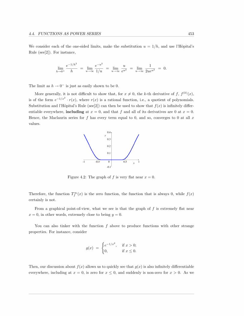
4.4. FUNCTIONS AS POWER SERIES 453
We consider each of the one-sided limits, make the substitution u = 1/h, and use l’Hopital’sRule (see[2]). For instance,
limh→0+
e−1/h2
h= lim
u→∞
e−u2
1/u= lim
u→∞
u
eu2 = limu→∞
12ueu2 = 0.
The limit as h→ 0− is just as easily shown to be 0.
More generally, it is not difficult to show that, for x 6= 0, the k-th derivative of f , f (k)(x),is of the form e−1/x2 · r(x), where r(x) is a rational function, i.e., a quotient of polynomials.Substitution and l’Hopital’s Rule (see[2]) can then be used to show that f(x) is infinitely differ-entiable everywhere, including at x = 0, and that f and all of its derivatives are 0 at x = 0.Hence, the Maclaurin series for f has every term equal to 0, and so, converges to 0 at all xvalues.
-1 -0.5 0 0.5 1
-0.1
0.1
0.2
0.3
0.4
Figure 4.2: The graph of f is very flat near x = 0.
Therefore, the function T∞f (x) is the zero function, the function that is always 0, while f(x)certainly is not.
From a graphical point-of-view, what we see is that the graph of f is extremely flat nearx = 0, in other words, extremely close to being y = 0.
You can also tinker with the function f above to produce functions with other strangeproperties. For instance, consider
g(x) =
{e−1/x2
, if x > 0;0, if x ≤ 0.
Then, our discussion about f(x) allows us to quickly see that g(x) is also infinitely differentiableeverywhere, including at x = 0, is zero for x ≤ 0, and suddenly is non-zero for x > 0. As we
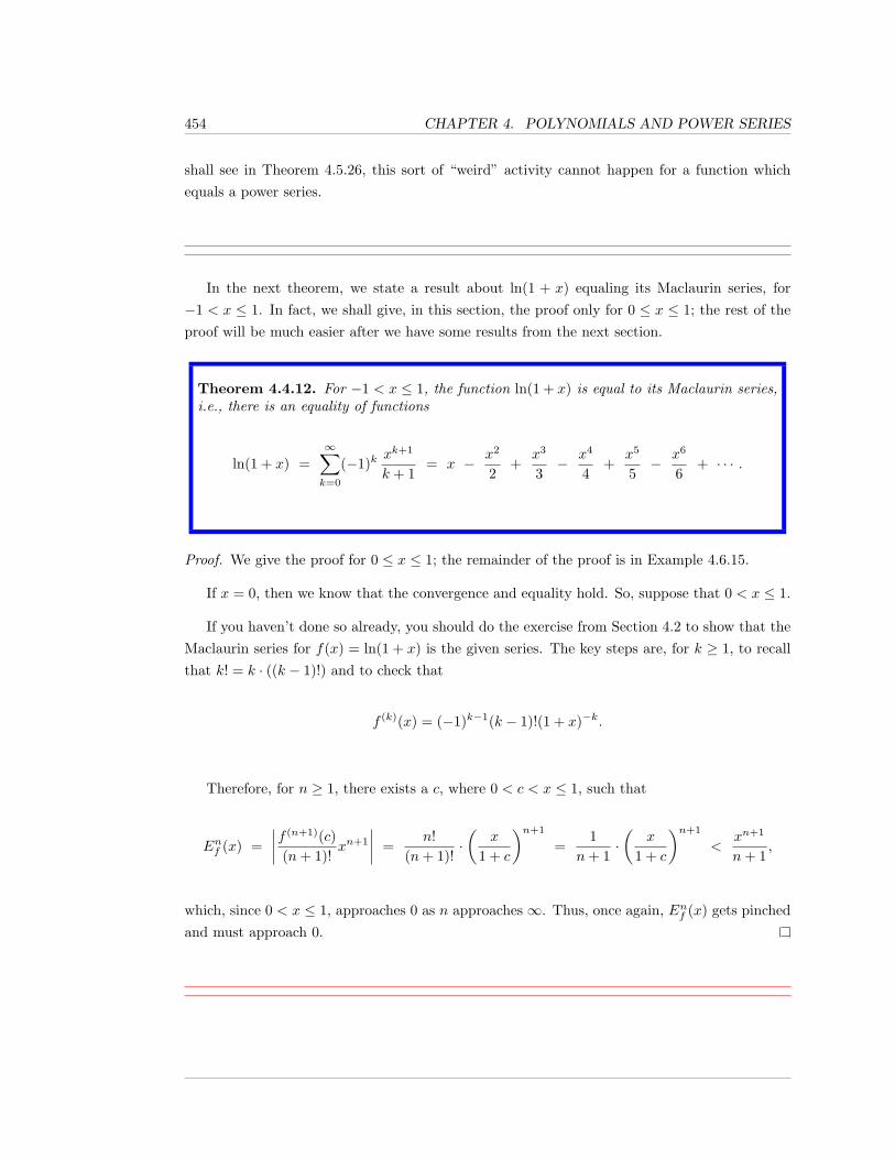
454 CHAPTER 4. POLYNOMIALS AND POWER SERIES
shall see in Theorem 4.5.26, this sort of “weird” activity cannot happen for a function whichequals a power series.
In the next theorem, we state a result about ln(1 + x) equaling its Maclaurin series, for−1 < x ≤ 1. In fact, we shall give, in this section, the proof only for 0 ≤ x ≤ 1; the rest of theproof will be much easier after we have some results from the next section.
Theorem 4.4.12. For −1 < x ≤ 1, the function ln(1 + x) is equal to its Maclaurin series,i.e., there is an equality of functions
ln(1 + x) =∞∑k=0
(−1)kxk+1
k + 1= x − x2
2+
x3
3− x4
4+
x5
5− x6
6+ · · · .
Proof. We give the proof for 0 ≤ x ≤ 1; the remainder of the proof is in Example 4.6.15.
If x = 0, then we know that the convergence and equality hold. So, suppose that 0 < x ≤ 1.
If you haven’t done so already, you should do the exercise from Section 4.2 to show that theMaclaurin series for f(x) = ln(1 + x) is the given series. The key steps are, for k ≥ 1, to recallthat k! = k · ((k − 1)!) and to check that
f (k)(x) = (−1)k−1(k − 1)!(1 + x)−k.
Therefore, for n ≥ 1, there exists a c, where 0 < c < x ≤ 1, such that
Enf (x) =∣∣∣∣f (n+1)(c)
(n+ 1)!xn+1
∣∣∣∣ =n!
(n+ 1)!·(
x
1 + c
)n+1
=1
n+ 1·(
x
1 + c
)n+1
<xn+1
n+ 1,
which, since 0 < x ≤ 1, approaches 0 as n approaches ∞. Thus, once again, Enf (x) gets pinchedand must approach 0.
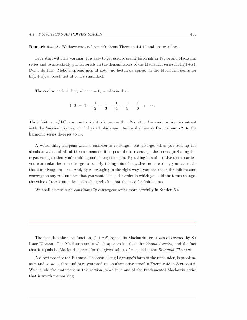
4.4. FUNCTIONS AS POWER SERIES 455
Remark 4.4.13. We have one cool remark about Theorem 4.4.12 and one warning.
Let’s start with the warning. It is easy to get used to seeing factorials in Taylor and Maclaurinseries and to mistakenly put factorials on the denominators of the Maclaurin series for ln(1+x).Don’t do this! Make a special mental note: no factorials appear in the Maclaurin series forln(1 + x), at least, not after it’s simplified.
The cool remark is that, when x = 1, we obtain that
ln 2 = 1 − 12
+13− 1
4+
15− 1
6+ · · · .
The infinite sum/difference on the right is known as the alternating harmonic series, in contrastwith the harmonic series, which has all plus signs. As we shall see in Proposition 5.2.16, theharmonic series diverges to ∞.
A weird thing happens when a sum/series converges, but diverges when you add up theabsolute values of all of the summands: it is possible to rearrange the terms (including thenegative signs) that you’re adding and change the sum. By taking lots of positive terms earlier,you can make the sum diverge to ∞. By taking lots of negative terms earlier, you can makethe sum diverge to −∞. And, by rearranging in the right ways, you can make the infinite sumconverge to any real number that you want. Thus, the order in which you add the terms changesthe value of the summation, something which is not the case for finite sums.
We shall discuss such conditionally convergent series more carefully in Section 5.4.
The fact that the next function, (1 + x)p, equals its Maclaurin series was discovered by SirIsaac Newton. The Maclaurin series which appears is called the binomial series, and the factthat it equals its Maclaurin series, for the given values of x, is called the Binomial Theorem.
A direct proof of the Binomial Theorem, using Lagrange’s form of the remainder, is problem-atic, and so we outline and have you produce an alternative proof in Exercise 43 in Section 4.6.We include the statement in this section, since it is one of the fundamental Maclaurin seriesthat is worth memorizing.
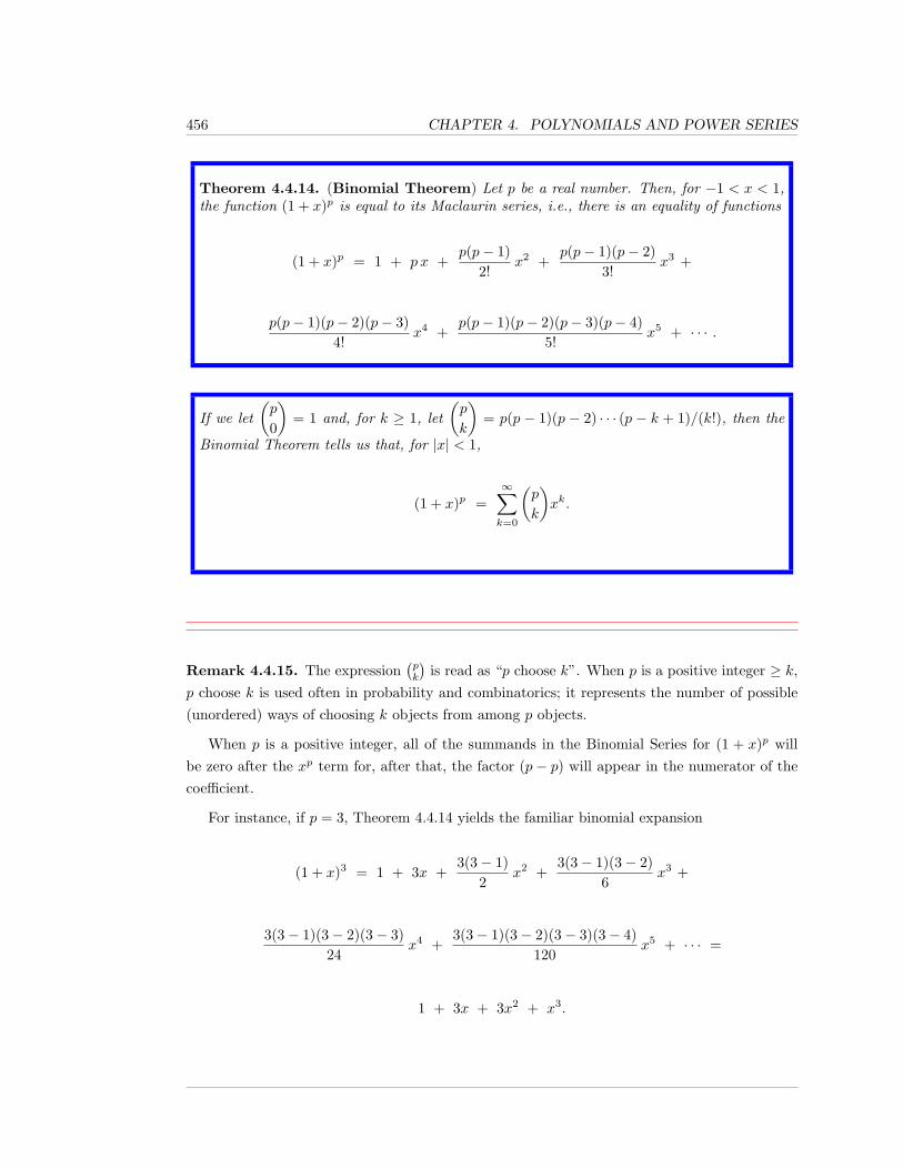
456 CHAPTER 4. POLYNOMIALS AND POWER SERIES
Theorem 4.4.14. (Binomial Theorem) Let p be a real number. Then, for −1 < x < 1,the function (1 + x)p is equal to its Maclaurin series, i.e., there is an equality of functions
(1 + x)p = 1 + p x +p(p− 1)
2!x2 +
p(p− 1)(p− 2)3!
x3 +
p(p− 1)(p− 2)(p− 3)4!
x4 +p(p− 1)(p− 2)(p− 3)(p− 4)
5!x5 + · · · .
If we let(p
0
)= 1 and, for k ≥ 1, let
(p
k
)= p(p − 1)(p − 2) · · · (p − k + 1)/(k!), then the
Binomial Theorem tells us that, for |x| < 1,
(1 + x)p =∞∑k=0
(p
k
)xk.
Remark 4.4.15. The expression(pk
)is read as “p choose k”. When p is a positive integer ≥ k,
p choose k is used often in probability and combinatorics; it represents the number of possible(unordered) ways of choosing k objects from among p objects.
When p is a positive integer, all of the summands in the Binomial Series for (1 + x)p willbe zero after the xp term for, after that, the factor (p− p) will appear in the numerator of thecoefficient.
For instance, if p = 3, Theorem 4.4.14 yields the familiar binomial expansion
(1 + x)3 = 1 + 3x +3(3− 1)
2x2 +
3(3− 1)(3− 2)6
x3 +
3(3− 1)(3− 2)(3− 3)24
x4 +3(3− 1)(3− 2)(3− 3)(3− 4)
120x5 + · · · =
1 + 3x + 3x2 + x3.
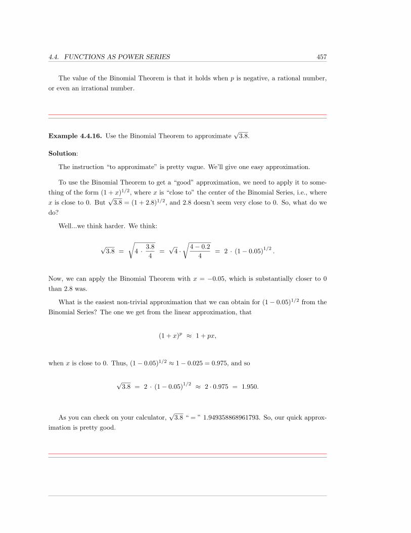
4.4. FUNCTIONS AS POWER SERIES 457
The value of the Binomial Theorem is that it holds when p is negative, a rational number,or even an irrational number.
Example 4.4.16. Use the Binomial Theorem to approximate√
3.8.
Solution:
The instruction “to approximate” is pretty vague. We’ll give one easy approximation.
To use the Binomial Theorem to get a “good” approximation, we need to apply it to some-thing of the form (1 + x)1/2, where x is “close to” the center of the Binomial Series, i.e., wherex is close to 0. But
√3.8 = (1 + 2.8)1/2, and 2.8 doesn’t seem very close to 0. So, what do we
do?
Well...we think harder. We think:
√3.8 =
√4 · 3.8
4=√
4 ·√
4− 0.24
= 2 · (1− 0.05)1/2.
Now, we can apply the Binomial Theorem with x = −0.05, which is substantially closer to 0than 2.8 was.
What is the easiest non-trivial approximation that we can obtain for (1− 0.05)1/2 from theBinomial Series? The one we get from the linear approximation, that
(1 + x)p ≈ 1 + px,
when x is close to 0. Thus, (1− 0.05)1/2 ≈ 1− 0.025 = 0.975, and so
√3.8 = 2 · (1− 0.05)1/2 ≈ 2 · 0.975 = 1.950.
As you can check on your calculator,√
3.8 “ = ” 1.949358868961793. So, our quick approx-imation is pretty good.
458 CHAPTER 4. POLYNOMIALS AND POWER SERIES
4.4.1 Exercises
1. Recall that
ln 2 = 1 − 12
+13− 1
4+
15− 1
6+
17− 1
8+
19− 1
10+ · · · .
Approximate ln 2 by using the partial sum containing the first 4 terms in the infinite series.Compare this with the calculator value of 0.693147180560 for ln 2. Would you say thatyour approximation is “good”? Does the approximation get better if you use the first 10terms?
2. a. Using that
ex = 1 + x+x2
2!+x3
3!+x4
4!+ · · · ,
we see that 6(ex − 1− x− x2
2
)is best approximated by what power of x when x is
close to 0?
b. Use your approximation from part (a) to estimate the value of
v = 6(e0.1 − 1− 0.1− (0.1)2
2
).
Compare your estimate with the value of v from your calculator.
3. a. Using that
sinx = x− x3
3!+x5
5!− x7
7!+ · · · ,
we see that x− sinx is best approximated by what function of the form cxn when x
is close to 0?
b. Use your approximation from part (a) to estimate the value of v = 0.1 − sin(0.1).Compare your estimate with the value of v from your calculator. (Make certain that
your calculator is set to use radians in trig functions.)
4. a. Using that
cosx = 1− x2
2!+x4
4!− x6
6!+ · · · ,
we see that 2(1− cosx) is best approximated by what power of x when x is close to0?
4.4. FUNCTIONS AS POWER SERIES 459
b. Use your approximation from part (a) to estimate the value of v = 2(1− cos(0.01)).Compare your estimate with the value of v from your calculator. (Make certain thatyour calculator is set to use radians in trig functions.)
5. a. Using that
ln(1 + x) = x − x2
2+
x3
3− x4
4+
x5
5− x6
6+ · · · .
we see that−x+ ln(1 + x)
x2is best approximated by what constant when x is close
to 0?
b. Without using l’Hopital’s Rule, calculate
limx→0
−x+ ln(1 + x)x2
.
6. a. We know that, for |x| < 1,
11− x
= 1 + x + x2 + x3 + x4 + · · · .
So, when x is close to zero, 1/(1− x) is best approximated by what quadratic poly-nomial?
b. Use your approximation in part (a) to estimate1
1.01. Compare this with the calcu-
lator value of 1/1.01.
7. The Binomial Theorem, Theorem 4.4.14, with p =13
, tells us that
(1 + x)1/3 = 1 +13x +
(13
) (− 2
3
)2!
x2 + · · · .
Use the first three terms of this series to estimate (1.09)1/3. Compare this with thecalculator value of (1.09)1/3.
460 CHAPTER 4. POLYNOMIALS AND POWER SERIES
8. Use the first two terms of the binomial series to approximate 5√
31, and compare this withthe value from your calculator.
9. Explain how the Binomial Theorem, Theorem 4.4.14, yields the Geometric Series Theorem,Theorem 4.4.10, in the case where a = 1.
10. a. Find the Taylor series for ex, centered at 5. Either use summation notation, or writeout the first 5 non-zero terms, followed by dots.
b. Determine the x values for which your Taylor series in part (a) equals the functionex
11. a. Find the Taylor series for cosx, centered at π/4. Either use summation notation, orwrite out the first 5 non-zero terms, followed by dots.
b. Determine the x values for which your Taylor series in part (a) equals the functioncosx
12. a. Find the Taylor series for sinx, centered at π/4. Either use summation notation, orwrite out the first 5 non-zero terms, followed by dots.
b. Determine the x values for which your Taylor series in part (a) equals the function
sinx.
13. a. Find the Taylor series for ln(1 + x), centered at 2. Either use summation notation,or write out the first 5 non-zero terms, followed by dots. Hint: You may wish to usethe formula for the k-th derivative from the proof of Theorem 4.4.12.
b. Can you determine any x values, other than 2, for which your Taylor series in part(a) equals the function ln(1 + x)?
14. a. Find the Taylor series for 1/(1 − x), centered at 2. Either use summation notation,or write out the first 5 non-zero terms, followed by dots.
b. Can you determine any x values, other than 2, for which your Taylor series in part(a) equals the function 1/(1− x)?
15. Let f(x) = xex.
a. Show that the k-th derivative of f , f (k)(x), is equal to (x+ k)ex.
b. Find the Maclaurin series for f(x), using the definition of Maclaurin series.
c. Why is your answer to part (b) unsurprising?
d. Show that f(x) is equal to its Maclaurin series for all x.
16. Suppose that f(x) is infinitely differentiable at 0. Then, g(x) = xf(x) is also infinitelydifferentiable at 0.
4.4. FUNCTIONS AS POWER SERIES 461
a. Show that, for k ≥ 1, g(k)(x) = xf (k)(x) + kf (k−1)(x).
b. Show that, if the Maclaurin series for f(x) is∑∞i=0 cix
i, then the Maclaurin series forg(x) is
∑∞i=0 cix
i+1.
c. Suppose that f(x) equals its Maclaurin series for all x in some set I. Show that g(x)equals its Maclaurin series for all x in I. (Hint: Do not use the Lagrange form of theremainder; use the definition of the Taylor remainder and the properties of limits.)
462 CHAPTER 4. POLYNOMIALS AND POWER SERIES
4.5 Power Series as Functions I:Definitions & the Ratio Test
In the previous section, we began with a function f(x) and discussed when it was equal to itsTaylor or Maclaurin series or, as people frequently say, when a given function can be representedby its Taylor series. We saw that f(x) = T∞f (x; a) if and only if the error Enf (x; a) approaches0 as n→∞.
Showing that the error approaches 0 actually implies two essentially separate things at once;it implies that T∞f (x, a) converges to something, and that the something that it converges tois precisely f(x).
But, what if you start with just a power series∑∞k=0 ck(x− a)k, instead of some pre-defined
function f(x)? Can we say when the power series, as a formal algebraic object, can be used todefine a function? And, even if we can use a power series to define a function, is there anypoint to doing so???
The answer to both of these questions is: YES. Power series define functions wherever theyconverge and, to a large extent, as far as algebraic operations, differentiation, and integrationare concerned, functions which are defined by power series can be treated just like polynomials,polynomials which never end.
In this section, we will begin our general investigation of using power series to define functions;though, actually, we introduced you to this idea in [2], when we defined the exponential functionexp(x) using limits of polynomials.
We shall give fundamental definitions and results on convergence, and the domain of apower series function. In particular, we will state and use the Ratio Test to find the radius ofconvergence, a fundamental notion related to the domains of power series functions. We shallalso define and discuss real analytic functions; these are functions which are locally equal topower series, but the center of the power series is allowed to move.
We will not prove the Ratio Test, or even state other convergence tests, until Chapter 5.However, before going into such an extensive discussion of convergence, we will, in the nextsection, Section 4.6, look at manipulations of convergent power series, in order to show why it’sso nice to have functions defined, or represented by, power series.
We discussed partial sums and convergence of Taylor series earlier (recall that the n-th orderpartial sum of a Taylor series is just the n-th order Taylor polynomial). These are special cases
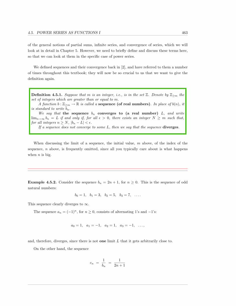
4.5. POWER SERIES AS FUNCTIONS I 463
of the general notions of partial sums, infinite series, and convergence of series, which we willlook at in detail in Chapter 5. However, we need to briefly define and discuss these terms here,so that we can look at them in the specific case of power series.
We defined sequences and their convergence back in [2], and have referred to them a numberof times throughout this textbook; they will now be so crucial to us that we want to give thedefinition again.
Definition 4.5.1. Suppose that m is an integer, i.e., is in the set Z. Denote by Z≥m theset of integers which are greater than or equal to m.
A function b : Z≥m → R is called a sequence (of real numbers). In place of b(n), itis standard to write bn.
We say that the sequence bn converges to (a real number) L, and writelimn→∞ bn = L if and only if, for all ε > 0, there exists an integer N ≥ m such that,for all integers n ≥ N , |bn − L| < ε.
If a sequence does not converge to some L, then we say that the sequence diverges.
When discussing the limit of a sequence, the initial value, m above, of the index of thesequence, n above, is frequently omitted, since all you typically care about is what happenswhen n is big.
Example 4.5.2. Consider the sequence bn = 2n + 1, for n ≥ 0. This is the sequence of oddnatural numbers:
b0 = 1, b1 = 3, b2 = 5, b3 = 7, . . . .
This sequence clearly diverges to ∞.
The sequence an = (−1)n, for n ≥ 0, consists of alternating 1’s and −1’s:
a0 = 1, a1 = −1, a2 = 1, a3 = −1, . . . ,
and, therefore, diverges, since there is not one limit L that it gets arbitrarily close to.
On the other hand, the sequence
cn =1bn
=1
2n+ 1
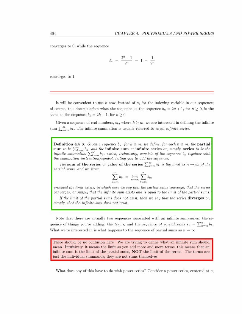
464 CHAPTER 4. POLYNOMIALS AND POWER SERIES
converges to 0, while the sequence
dn =2n − 1
2n= 1 − 1
2n
converges to 1.
It will be convenient to use k now, instead of n, for the indexing variable in our sequence;of course, this doesn’t affect what the sequence is; the sequence bn = 2n + 1, for n ≥ 0, is thesame as the sequence bk = 2k + 1, for k ≥ 0.
Given a sequence of real numbers, bk, where k ≥ m, we are interested in defining the infinitesum
∑∞k=m bk. The infinite summation is usually referred to as an infinite series.
Definition 4.5.3. Given a sequence bk, for k ≥ m, we define, for each n ≥ m, the partialsum to be
∑nk=m bk, and the infinite sum or infinite series or, simply, series to be the
infinite summation∑∞k=m bk, which, technically, consists of the sequence bk together with
the summation instruction/symbol, telling you to add the sequence.The sum of the series or value of the series
∑∞k=m bk is the limit as n→∞ of the
partial sums, and we write∞∑k=m
bk = limn→∞
n∑k=m
bk,
provided the limit exists, in which case we say that the partial sums converge, that the seriesconverges, or simply that the infinite sum exists and is equal to the limit of the partial sums.
If the limit of the partial sums does not exist, then we say that the series diverges or,simply, that the infinite sum does not exist.
Note that there are actually two sequences associated with an infinite sum/series: the se-quence of things you’re adding, the terms, and the sequence of partial sums sn =
∑nk=m bk.
What we’re interested in is what happens to the sequence of partial sums as n→∞.
There should be no confusion here. We are trying to define what an infinite sum shouldmean. Intuitively, it means the limit as you add more and more terms; this means that aninfinite sum is the limit of the partial sums, NOT the limit of the terms. The terms arejust the individual summands; they are not sums themselves.
What does any of this have to do with power series? Consider a power series, centered at a,
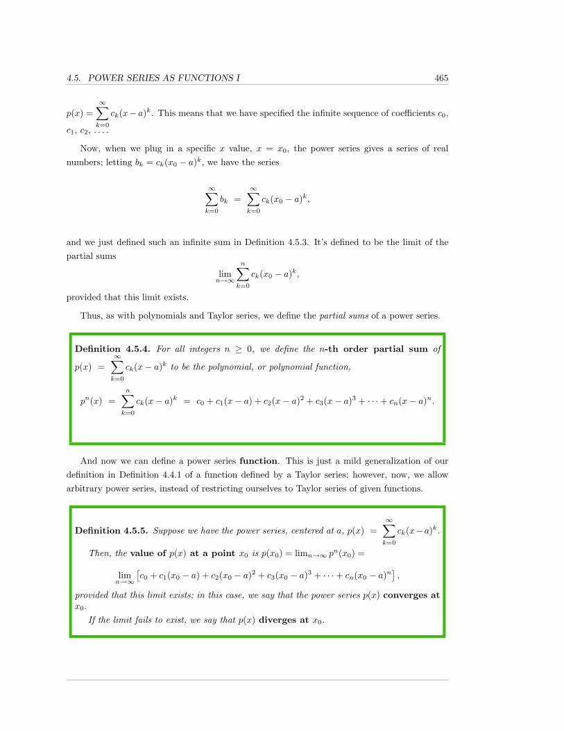
4.5. POWER SERIES AS FUNCTIONS I 465
p(x) =∞∑k=0
ck(x− a)k. This means that we have specified the infinite sequence of coefficients c0,
c1, c2, . . . .
Now, when we plug in a specific x value, x = x0, the power series gives a series of realnumbers; letting bk = ck(x0 − a)k, we have the series
∞∑k=0
bk =∞∑k=0
ck(x0 − a)k,
and we just defined such an infinite sum in Definition 4.5.3. It’s defined to be the limit of thepartial sums
limn→∞
n∑k=0
ck(x0 − a)k,
provided that this limit exists.
Thus, as with polynomials and Taylor series, we define the partial sums of a power series.
Definition 4.5.4. For all integers n ≥ 0, we define the n-th order partial sum of
p(x) =∞∑k=0
ck(x− a)k to be the polynomial, or polynomial function,
pn(x) =n∑k=0
ck(x− a)k = c0 + c1(x− a) + c2(x− a)2 + c3(x− a)3 + · · ·+ cn(x− a)n.
And now we can define a power series function. This is just a mild generalization of ourdefinition in Definition 4.4.1 of a function defined by a Taylor series; however, now, we allowarbitrary power series, instead of restricting ourselves to Taylor series of given functions.
Definition 4.5.5. Suppose we have the power series, centered at a, p(x) =∞∑k=0
ck(x−a)k.
Then, the value of p(x) at a point x0 is p(x0) = limn→∞ pn(x0) =
limn→∞
[c0 + c1(x0 − a) + c2(x0 − a)2 + c3(x0 − a)3 + · · ·+ cn(x0 − a)n
],
provided that this limit exists; in this case, we say that the power series p(x) converges atx0.
If the limit fails to exist, we say that p(x) diverges at x0.
466 CHAPTER 4. POLYNOMIALS AND POWER SERIES
The power series function p(x) is the function whose domain is the set of x0 at which p(x)converges, and its value at any x0 in its domain is p(x0), as defined above. The codomainof a power series function is taken to be all real numbers. The notation for this function isthe same as that of the algebraic power series, p(x), and we frequently use the term “powerseries” to mean either the formal algebraic series or the function, letting the context makethe distinction clear.
Remark 4.5.6. It is trivial, but important, that every power series, centered at a, convergesat x = a; for there, the value of every term, other than the constant term, is zero, and so everypartial sum is simply the constant term c0. Thus,
p(a) = limn→∞
pn(a) = limn→∞
c0 = c0.
The real question is: where else, besides the center, does the power series converge?
Example 4.5.7. Recall from Section 4.4 that the Maclaurin series for ex, sinx, and cosx are,respectively,
∞∑k=0
xk
k!,
∞∑k=0
(−1)kx2k+1
(2k + 1)!, and
∞∑k=0
(−1)kx2k
(2k)!.
In fact, in Section 4.4, we did not consider the separate question of which x values make theseseries converge; we looked only at the question of which x values make the series converge and
make what they converge to equal to the value of the original function.
However, the three power series above converge and equal the original function for all x andso, in particular the domain of each of the three power series functions above is the entire realline (−∞,∞).
In Section 4.4, we also saw that the domain of the Maclaurin series (function) of a/(1−x), fora 6= 0, is precisely (−1, 1), for, in Theorem 4.4.10, we included the statement that the Maclaurinseries diverges outside of the interval (−1, 1).
On the other hand, you have to be somewhat careful when looking back at Section 4.4 forthe domains of the Maclaurin series of ln(1 + x) and (1 + x)p. In Section 4.4, we gave intervals
4.5. POWER SERIES AS FUNCTIONS I 467
on which the Maclaurin series of these two functions are equal to the functions themselves, butthere was no claim that the Maclaurin series diverged outside of those intervals; in theory, thesets of points on which the Maclaurin series converge could be larger than the intervals on whichthe Maclaurin series agree with the original functions.
As we shall see later, the domain of the Maclaurin series function of ln(1 + x) is preciselythe interval on which the series converges to ln(1 + x), namely, the interval (−1, 1].
However, the domain of the Maclaurin series function of (1+x)p, the binomial series, dependson p, and can be any one of three possible intervals: (−1, 1), (−1, 1], or [−1, 1]. While it is beyondthe scope of this textbook, it can be shown that the binomial series for (1 + x)p converges atx = −1 if and only if p ≥ 0, and converges at x = 1 if and only if p > −1. Thus, for instance,when p = −1/2, the interval on which the Maclaurin series of 1/
√1 + x converges is (−1, 1].
Of course, we haven’t given an example of a power series that’s not the Maclaurin series ofsome “nice” function. What can we say about the domain of the power series function
∞∑k=1
(x− 5)k
3kk2=
13
(x− 5) +1
32 · 22(x− 5)2 +
133 · 32
(x− 5)3 +1
34 · 42(x− 5)4 + . . .?
Below, we give a general result that tells us that the domain of this, or any, power seriesfunction must be an interval, and, in fact, that interval must have, as its center, the center ofthe power series, which is 5 for the series above. We will then state the Ratio Test, which tellsyou, in many cases, how to find the radius (half the length) of the interval on which the seriesconverges.
Recall now that an extended real number is a real number or ±∞. We need one moredefinition before we can begin with the results and examples.
Definition 4.5.8. Suppose that R ≥ 0 is an extended real number, i.e., a non-negative realnumber or ∞.
Then, an interval centered at a is an interval which contains a and which has end-points a − R and a + R, where the interval may or may not include one or both of theendpoints.
Note that, if R = ∞, then the interval is (−∞,∞), and if R = 0, then the interval(which was required to contain a) must be the closed interval which contains only a, i.e.,must be [a, a].
The extended real number R is called the radius of the interval.
468 CHAPTER 4. POLYNOMIALS AND POWER SERIES
As we mentioned, back in Example 4.5.7, there is the following result.
Theorem 4.5.9. The set of points at which a power series,∑∞k=0 ck(x − a)k, centered at
a, converges is an interval centered at a.In addition, at points x in the interior of this interval (if there are any), the series∑∞k=0 |ck| · |x− a|k, whose terms are the absolute values of the original series, converges.
Proof. This result is beyond the scope of this textbook. See Theorem 4.5.2 of [4].
In light of this, we make another definition.
Definition 4.5.10. The interval of points at which a power series converges, that is, thedomain of the power series function, is called the interval of convergence of the powerseries, and the radius of that interval is called the radius of convergence of the powerseries.
Thus, for a power series∑∞k=0 ck(x− a)k centered at a, the radius of convergence is the
unique extended real number R ≥ 0 such that, if |x− a| < R, then the series converges, andif |x− a| > R, then the series diverges.
Remark 4.5.11. The second paragraph of Theorem 4.5.9 means that, when R > 0, at pointswhere |x − a| < R, i.e., at points x in the open interval (a − R, a + R) (meaning the openinterval (−∞,∞), when R =∞), the power series converges in a fairly strong way; it convergesabsolutely, which we won’t discuss any further until Section 5.4.
Example 4.5.12. In Example 4.5.7, using our current terminology, what we saw is that theintervals of convergence of the Maclaurin series for ex, sinx, and cosx are all (−∞,∞) and,hence, the radii of convergence for all of those series are ∞.
We also discussed in Example 4.5.7 that, for a 6= 0, the Maclaurin series for a/(1−x), i.e., thegeometric series, has (−1, 1) as its interval of convergence, and so, has radius of convergence 1.Furthermore, the Maclaurin series for ln(1+x) and (1+x)p also have radii of convergence equalto 1, with corresponding intervals of convergence (−1, 1] and, depending on p, one of (−1, 1),(−1, 1], and [−1, 1].

4.5. POWER SERIES AS FUNCTIONS I 469
However, we have yet to explain any method whatsoever for determining the radius or intervalof convergence of essentially arbitrary series, like
∑∞k=1
(x−5)k
3kk2 from Example 4.5.7. For this, weuse the Ratio Test, below.
There are many theorems related to the convergence of power series; by far the most impor-tant of these is the Ratio Test. We shall discuss the Ratio Test in this section, and defer theother convergence tests until Chapter 5. The Ratio Test is a theorem about series of constants,but which, when applied to many power series, yields the radii of convergence. However, theRatio Test, in its usual form, can never tell you about convergence/divergence at the endpointsof the interval of convergence.
As we shall see in Theorem 5.3.23, the proof of the Ratio Test just amounts to comparingwith what happens for geometric series (recall Theorem 4.4.10).
Theorem 4.5.13. (The Ratio Test) Consider the series∞∑k=m
bk.
1. If there exists r < 1 (and, necessarily, > 0) and an integer M ≥ m such that, for allk ≥M ,
bk 6= 0 and∣∣∣∣bk+1
bk
∣∣∣∣ ≤ r,then the given series converges.
2. If there exists an integer M ≥ m such that, for all k ≥M ,
bk 6= 0 and∣∣∣∣bk+1
bk
∣∣∣∣ ≥ 1,
then the given series diverges.
In particular, suppose that limk→∞
∣∣∣∣bk+1
bk
∣∣∣∣ exists, as an extended real number; call its value L.
Then,
a. if L < 1, the given series converges;
b. if L > 1, including L =∞, the given series diverges;
c. if L = 1, the given series may converge or diverge.
470 CHAPTER 4. POLYNOMIALS AND POWER SERIES
Remark 4.5.14. You usually try to calculate the limit L in the Ratio Test first, and hope thatit exists and is unequal to 1. If L fails to exist or equals 1, then you consider cases 1) and 2).
Be aware, however, that, if L exists and L = 1, then there cannot possibly exist an r as incase 1) of the Ratio Test, and so you will not be able to use the Ratio Test to conclude that theseries converges. On the other hand, even if L = 1, you may be able to use case 2) to concludethat the series diverges.
Also, if the limit L fails to exist, cases 1) and 2) may enable you to conclude convergence ordivergence of a given infinite series.
Remark 4.5.15. Due to the nature of the Ratio Test and because factorials frequently appearin series, it is worth recalling how factorials work, before we look at examples.
From the definition, for k ≥ 0,
(k + 1)! = (k + 1)k(k − 1)(k − 2) · · · (3)(2)(1)
and(2k + 2)! = (2k + 2)(2k + 1)(2k)(2k − 1)(2k − 2) · · · (3)(2)(1).
Hence,(k + 1)! = (k + 1)(k!) and [2(k + 1)]! = (2k + 2)(2k + 1)[(2k)!],
and so(k + 1)!k!
= k + 1 and[2(k + 1)]!
(2k)!= (2k + 2)(2k + 1).
The point of this is not that you should memorize these specific formulas for quotients involvingfactorials, but rather that, if you just think about what factorial means, such formulas becomequick and easy to derive.
Example 4.5.16. Let’s consider six different series of constants, series whose terms, for k ≥ 1,are given by
ak =13k, bk = 3k, ck =
3k
k!, dk = (−1)kk, ek =
1k, and fk =
(−1)k+1
k.
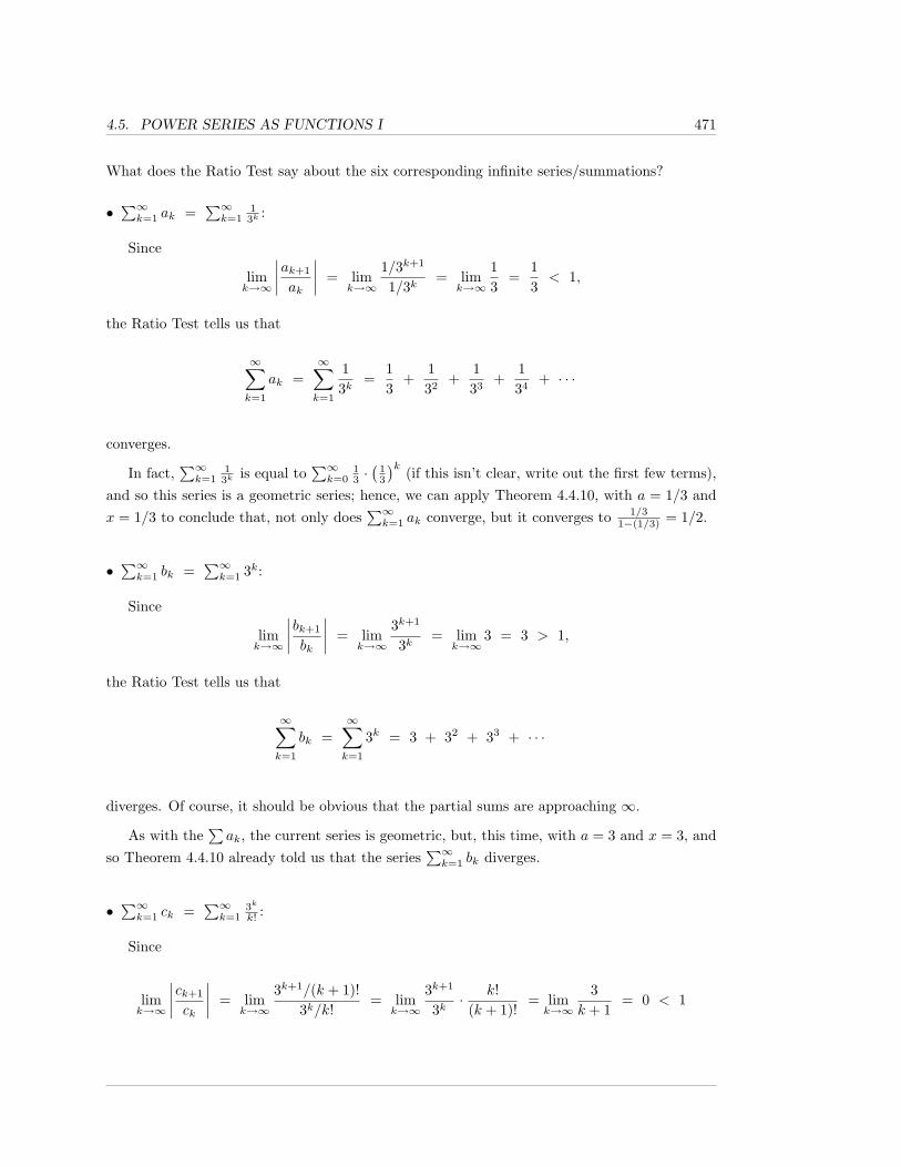
4.5. POWER SERIES AS FUNCTIONS I 471
What does the Ratio Test say about the six corresponding infinite series/summations?
•∑∞k=1 ak =
∑∞k=1
13k
:
Since
limk→∞
∣∣∣∣ak+1
ak
∣∣∣∣ = limk→∞
1/3k+1
1/3k= lim
k→∞
13
=13< 1,
the Ratio Test tells us that
∞∑k=1
ak =∞∑k=1
13k
=13
+132
+133
+134
+ · · ·
converges.
In fact,∑∞k=1
13k
is equal to∑∞k=0
13 ·(
13
)k (if this isn’t clear, write out the first few terms),and so this series is a geometric series; hence, we can apply Theorem 4.4.10, with a = 1/3 andx = 1/3 to conclude that, not only does
∑∞k=1 ak converge, but it converges to 1/3
1−(1/3) = 1/2.
•∑∞k=1 bk =
∑∞k=1 3k:
Since
limk→∞
∣∣∣∣bk+1
bk
∣∣∣∣ = limk→∞
3k+1
3k= lim
k→∞3 = 3 > 1,
the Ratio Test tells us that
∞∑k=1
bk =∞∑k=1
3k = 3 + 32 + 33 + · · ·
diverges. Of course, it should be obvious that the partial sums are approaching ∞.
As with the∑ak, the current series is geometric, but, this time, with a = 3 and x = 3, and
so Theorem 4.4.10 already told us that the series∑∞k=1 bk diverges.
•∑∞k=1 ck =
∑∞k=1
3k
k! :
Since
limk→∞
∣∣∣∣ck+1
ck
∣∣∣∣ = limk→∞
3k+1/(k + 1)!3k/k!
= limk→∞
3k+1
3k· k!
(k + 1)!= limk→∞
3k + 1
= 0 < 1
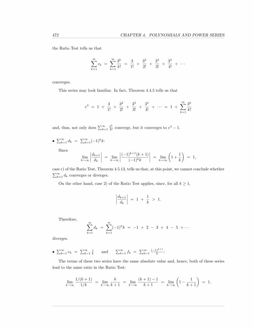
472 CHAPTER 4. POLYNOMIALS AND POWER SERIES
the Ratio Test tells us that
∞∑k=1
ck =∞∑k=1
3k
k!=
31!
+32
2!+
33
3!+
34
4!+ · · ·
converges.
This series may look familiar. In fact, Theorem 4.4.5 tells us that
e3 = 1 +31!
+32
2!+
33
3!+
34
4!+ · · · = 1 +
∞∑k=1
3k
k!
and, thus, not only does∑∞k=1
3k
k! converge, but it converges to e3 − 1.
•∑∞k=1 dk =
∑∞k=1(−1)kk:
Since
limk→∞
∣∣∣∣dk+1
dk
∣∣∣∣ = limk→∞
∣∣∣∣ (−1)k+1(k + 1)(−1)kk
∣∣∣∣ = limk→∞
(1 +
1k
)= 1,
case c) of the Ratio Test, Theorem 4.5.13, tells us that, at this point, we cannot conclude whether∑∞k=1 dk converges or diverges.
On the other hand, case 2) of the Ratio Test applies, since, for all k ≥ 1,
∣∣∣∣dk+1
dk
∣∣∣∣ = 1 +1k> 1.
Therefore,∞∑k=1
dk =∞∑k=1
(−1)kk = −1 + 2 − 3 + 4 − 5 + · · ·
diverges.
•∑∞k=1 ek =
∑∞k=1
1k and
∑∞k=1 fk =
∑∞k=1
(−1)k+1
k :
The terms of these two series have the same absolute value and, hence, both of these serieslead to the same ratio in the Ratio Test:
limk→∞
1/(k + 1)1/k
= limk→∞
k
k + 1= lim
k→∞
(k + 1)− 1k + 1
= limk→∞
(1− 1
k + 1
)= 1.
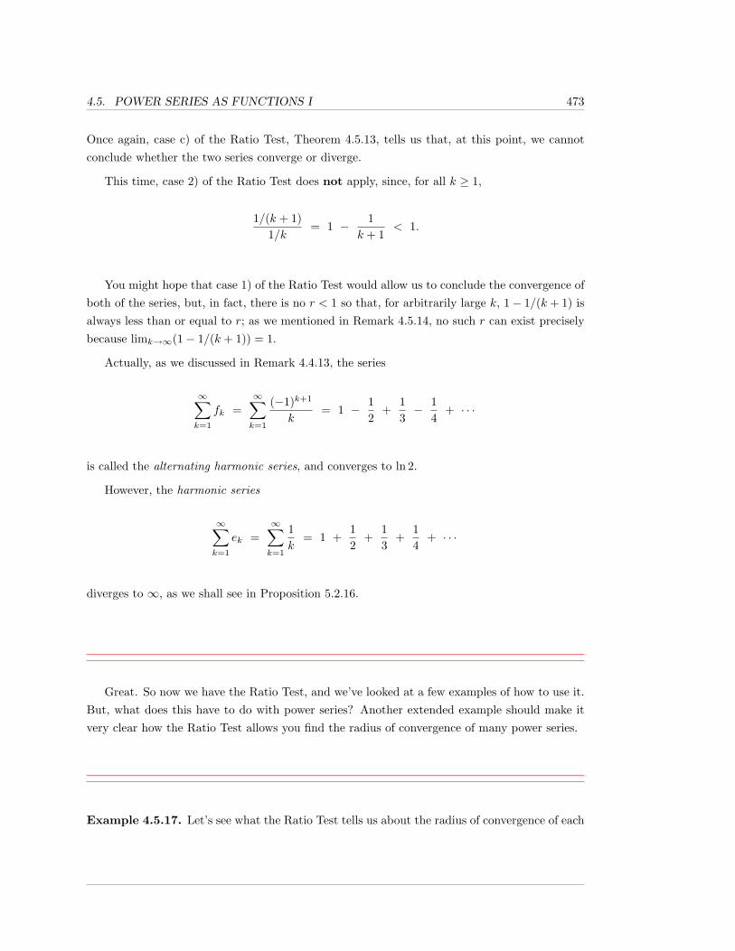
4.5. POWER SERIES AS FUNCTIONS I 473
Once again, case c) of the Ratio Test, Theorem 4.5.13, tells us that, at this point, we cannotconclude whether the two series converge or diverge.
This time, case 2) of the Ratio Test does not apply, since, for all k ≥ 1,
1/(k + 1)1/k
= 1 − 1k + 1
< 1.
You might hope that case 1) of the Ratio Test would allow us to conclude the convergence ofboth of the series, but, in fact, there is no r < 1 so that, for arbitrarily large k, 1− 1/(k + 1) isalways less than or equal to r; as we mentioned in Remark 4.5.14, no such r can exist preciselybecause limk→∞(1− 1/(k + 1)) = 1.
Actually, as we discussed in Remark 4.4.13, the series
∞∑k=1
fk =∞∑k=1
(−1)k+1
k= 1 − 1
2+
13− 1
4+ · · ·
is called the alternating harmonic series, and converges to ln 2.
However, the harmonic series
∞∑k=1
ek =∞∑k=1
1k
= 1 +12
+13
+14
+ · · ·
diverges to ∞, as we shall see in Proposition 5.2.16.
Great. So now we have the Ratio Test, and we’ve looked at a few examples of how to use it.But, what does this have to do with power series? Another extended example should make itvery clear how the Ratio Test allows you find the radius of convergence of many power series.
Example 4.5.17. Let’s see what the Ratio Test tells us about the radius of convergence of each
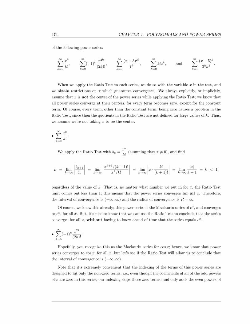
474 CHAPTER 4. POLYNOMIALS AND POWER SERIES
of the following power series:
∞∑k=0
xk
k!,
∞∑k=0
(−1)kx2k
(2k)!,
∞∑k=0
(x+ 3)2k
7k,
∞∑k=0
k!xk, and∞∑k=1
(x− 5)k
3kk2.
When we apply the Ratio Test to each series, we do so with the variable x in the test, andwe obtain restrictions on x which guarantee convergence. We always explicitly, or implicitly,assume that x is not the center of the power series while applying the Ratio Test; we know thatall power series converge at their centers, for every term becomes zero, except for the constantterm. Of course, every term, other than the constant term, being zero causes a problem in theRatio Test, since then the quotients in the Ratio Test are not defined for large values of k. Thus,we assume we’re not taking x to be the center.
•∞∑k=0
xk
k!:
We apply the Ratio Test with bk =xk
k!(assuming that x 6= 0), and find
L = limk→∞
∣∣∣∣bk+1
bk
∣∣∣∣ = limk→∞
∣∣∣∣xk+1/(k + 1)!xk/k!
∣∣∣∣ = limk→∞
∣∣∣∣x · k!(k + 1)!
∣∣∣∣ = limk→∞
|x|k + 1
= 0 < 1,
regardless of the value of x. That is, no matter what number we put in for x, the Ratio Testlimit comes out less than 1; this means that the power series converges for all x. Therefore,the interval of convergence is (−∞,∞) and the radius of convergence is R =∞.
Of course, we knew this already; this power series is the Maclaurin series of ex, and convergesto ex, for all x. But, it’s nice to know that we can use the Ratio Test to conclude that the seriesconverges for all x, without having to know ahead of time that the series equals ex.
•∞∑k=0
(−1)kx2k
(2k)!:
Hopefully, you recognize this as the Maclaurin series for cosx; hence, we know that powerseries converges to cosx, for all x, but let’s see if the Ratio Test will allow us to conclude thatthe interval of convergence is (−∞,∞).
Note that it’s extremely convenient that the indexing of the terms of this power series aredesigned to hit only the non-zero terms, i.e., even though the coefficients of all of the odd powersof x are zero in this series, our indexing skips those zero terms, and only adds the even powers of
4.5. POWER SERIES AS FUNCTIONS I 475
x. Missing the non-zero terms makes the ratios in the Ratio Test defined, since we don’t divideby zero.
We apply the Ratio Test and calculate
L = limk→∞
∣∣∣∣x2(k+1)/[2(k + 1)]!x2k/(2k)!
∣∣∣∣ = limk→∞
(x2 · (2k)!
(2k + 2)!
)= lim
k→∞
x2
(2k + 2)(2k + 1)= 0 < 1,
regardless of the value of x. So, yes, once again the Ratio Test allows us to conclude that theinterval of convergence is the entire real line (−∞,∞), and so the radius of convergence is ∞.
•∞∑k=0
(x+ 3
7
)k=
∞∑k=0
17k
(x+ 3)k:
We apply the Ratio Test and calculate
L = limk→∞
∣∣∣∣ (x+ 3)k+1/7k+1
(x+ 3)k/7k
∣∣∣∣ = limk→∞
|x+ 3|7
=|x+ 3|
7.
Now, the Ratio Test tells us that the series converges if |x+ 3|/7 < 1 and diverges if |x+ 3| > 1.Multiplying by 7, we find that the series, which is centered at −3, converges if |x − (−3)| < 7and diverges if |x − (−3)| > 7; looking back at Definition 4.5.10, you can see that this tells usthat the radius of convergence of the series is 7.
Thus, the largest open interval on which the series converges is the interval (−3−7,−3+7) =(−10, 4), but this easy use of the Ratio Test does not tell you what happens at the endpoints ofthis interval, for the endpoints are exactly where the limit in the Ratio Test comes out to equal1. This specific example shows you what happens in general: when you apply the Ratio Test,Theorem 4.5.13, simply calculating the limit L in cases a), b), and c) can never tell you aboutconvergence/divergence at the endpoints of the interval of convergence.
However, in this particular example, case 2) of Ratio Test allows us to conclude that theseries diverges at both endpoints of the interval of convergence. This isn’t terribly surprising;the proof of the Ratio Test uses that we know exactly what happens for geometric series and,while it’s slightly disguised, the series
∑∞k=0
(x+3
7
)k is, in fact, geometric.
How do you see this? Well...the most basic geometric series, when a = 1 in Theorem 4.4.10,is
11− x
=∞∑k=0
xk,
where the equality holds for |x| < 1, and the series diverges for |x| ≥ 1. Replacing the x
476 CHAPTER 4. POLYNOMIALS AND POWER SERIES
everywhere with the quantity (x+ 3)/7, we find that
11− x+3
7
=∞∑k=0
(x+ 3
7
)k,
where the equality holds for∣∣x+3
7
∣∣ < 1, and the series diverges for∣∣x+3
7
∣∣ ≥ 1. Note that theconvergence/divergence is exactly what we found by using the Ratio Test.
•∞∑k=0
k!xk:
We calculate the limit L from the Ratio Test:
L = limk→∞
∣∣∣∣ (k + 1)!xk+1
k!xk
∣∣∣∣ = limk→∞
(k + 1)|x|.
If x 6= 0, this limit is ∞, which is greater than 1, regardless of the value of x. Thus, the RatioTest tells us that this series converges only at the center x = 0 or, equivalently, that the radiusof convergence is 0.
•∞∑k=1
(x− 5)k
3kk2:
We calculate the limit L from the Ratio Test:
L = limk→∞
∣∣∣∣∣∣(x−5)k+1
3k+1(k+1)2
(x−5)k
3kk2
∣∣∣∣∣∣ = limk→∞
∣∣∣∣ (x− 5)k+1
(x− 5)k· 3k
3k+1· k2
(k + 1)2
∣∣∣∣ =|x− 5|
3limk→∞
(k
k + 1
)2
.
Dividing by k in the numerator and denominator inside the parentheses, we find
L =|x− 5|
3limk→∞
(1
1 + 1k
)2
=|x− 5|
3.
Therefore, the series converges when |x−5|/3 < 1 and diverges when |x−5|/3 > 1, i.e., convergeswhen |x− 5| < 3 and diverges when |x− 5| > 3. Hence, the radius of convergence is 3, and thelargest open interval on which the series converges is the interval (5− 3, 5 + 3) = (2, 8).
4.5. POWER SERIES AS FUNCTIONS I 477
We leave it as an exercise for you to show that even the more-complicated parts of the RatioTest do not allow you to conclude anything about convergence/divergence when x = 2 andx = 8.
One final note on applying the Ratio Test to this last series: as we saw, it can be veryhelpful to split up the quotient that appears in the Ratio Test into a product of quotients ofsimilar-looking terms. The calculation of the limits frequently works out nicely when you dothis.
Remark 4.5.18. You may have figured out from the above examples how to calculate theradius of convergence the “easy way”; the Ratio Test implies that, if you have the infinite series∑∞k=0 ck(x− a)k, and
limk→∞
∣∣∣∣ ckck+1
∣∣∣∣ = R,
where R is an extended real number, then R is the radius of convergence of the power series.
Example 4.5.19. Consider the last series from Example 4.5.17:∞∑k=1
(x− 5)k
3kk2.
We calculate
R = limk→∞
∣∣∣∣∣ 1/(3kk2
)1/ (3k+1(k + 1)2)
∣∣∣∣∣ = limk→∞
3k+1
3k· (k + 1)2
k2= 3,
as we found in Example 4.5.17.
It’s important when using the method of Remark 4.5.18 that the limit limk→∞
∣∣∣∣ ckck+1
∣∣∣∣ exists,
at least as an extended real number, and that ck is the coefficient of (x − a)k, i.e., that you’relooking at all of the powers of (x− a).
Consider, for instance, the series
∞∑k=0
(x+ 7)2k
9k= 1 +
(x+ 7)2
9+
(x+ 7)4
92+
(x+ 7)6
93+ · · · .
478 CHAPTER 4. POLYNOMIALS AND POWER SERIES
Note that the odd terms are missing. It might be tempting to think that the radius of convergencecan be calculated from the coefficients of the non-zero terms, and look at
limk→∞
∣∣∣∣ 1/9k
1/9k+1
∣∣∣∣ = 9.
However, the radius of convergence is not 9. Why not?
You can apply the Ratio Test to the series and determine that the series converges when|x+ 7|2
9< 1 and diverges when
|x+ 7|2
9> 1. Therefore, the radius of convergence is
√9 = 3.
In general, it is not particularly interesting to have functions defined by power series thatconverge only at their centers; such a function has a single point in its domain and, at thatsingle point, the function equals the constant term in the series. Not too useful.
Therefore, our interest is really in functions which equal power series on a non-empty openinterval around the center a of the series. As we shall see in the next section, this necessarilymeans that the function equals its Taylor series, centered at a. We give a name to such functions.
Definition 4.5.20. Suppose that f is an infinitely differentiable function on an open subsetU of R. Let V be an open subset of U , and let a be a point in U .
Then, f(x) is real analytic at a provided that, for all x in some open interval arounda, T∞f (x; a) converges to f(x). This is equivalent to saying that f(x) is equal to some(convergent) power series, centered at a, on an open interval containing a.
The function f is said to be real analytic on V provided that f is real analytic at x,for all x in V. A function which is real analytic on its whole domain is simply called a realanalytic function.
Example 4.5.21. Suppose that we have a power series p(x) =∑∞k=0 ck(x− a)k, centered at a,
with a positive radius of convergence R > 0. Then, the function defined by p(x), on the intervalof convergence of p(x), is, by definition, real analytic at a, since p(x) equals the convergentpower series
∑∞k=0 ck(x− a)k on (at least) the non-empty open interval (a−R, a+R).
4.5. POWER SERIES AS FUNCTIONS I 479
Remark 4.5.22. There is a subtle, but extremely important, point in the definition of a functionbeing real analytic on an open subset or, more specifically, on an open interval.
Suppose that f is real analytic at a. This means that there exists an open interval I, arounda, such that, for all x in I, f(x) = T∞f (x; a) or, equivalently, that there is some power series∑∞k=0 ck(x− a)k such that f(x) =
∑∞k=0 ck(x− a)k on a non-empty open interval I around a.
The question is: does this mean that f is real analytic on I, i.e., if b is in I, must it be truethat f is real analytic at b?
Your tendency might be to say “Sure – f equals its Taylor series for all x in I, and b is in I,so f equals its Taylor series at b”.
The problem here is that what we mean by “its Taylor series” should not be the same bothtimes in the sentence above. The first time that we wrote “its Taylor series”, we meant “itsTaylor series centered at a”. However, f being real analytic at b means that the Taylor seriesof f , centered at b, converges to f(x) for all x in an open interval around b. In other words,being real analytic at different points requires you to switch the center of your Taylor/powerseries to match the point under consideration, and then you need that the Taylor series T∞f (x; b)around this (possibly) new center b also converges to f(x) on some open interval around b; thisinterval around b need not be the same open interval I on which T∞f (x; a) converged.
Fortunately, there is a theorem, Theorem 8.4 of [3], which tells us that, in fact, we don’treally have to worry about the subtle point discussed above.
Theorem 4.5.23. Let R be a positive extended real number. Suppose that T∞f (x; a) con-verges to f(x) for all x in the open interval I defined by |x− a| < R. Then, for all b in I,T∞f (x; b) converges to f(x) for all x such that |x− b| < R− |b− a|, that is, for all x in thelargest open interval, centered at b, which is contained in I.
As a special case, if T∞f (x; a) converges to f(x) for all real numbers x, then so doesT∞f (x; b), for every real number b.
In particular, if T∞f (x; a), or any power series∑∞k=0 ck(x − a)k, converges to f(x) for
all x in an open interval I, centered at a, then f is real analytic on I.
Example 4.5.24. We know that ex, sinx, and cosx are equal to their Maclaurin series, for allx. Theorem 4.5.23 tells us that being equal to their Maclaurin series on the interval (−∞,∞) in
480 CHAPTER 4. POLYNOMIALS AND POWER SERIES
fact implies that, on the entire real line, these functions are equal to their Taylor series centered
anywhere. Of course, we could have determined this by showing that the Taylor error, withan arbitrary center, approaches zero, but Theorem 4.5.23 gives it to us without any additionalwork.
Example 4.5.25. Let’s look at a function which has a Maclaurin series with a positive, finiteradius of convergence. Consider the function f(x) = ln(1 + x), for all x > −1. Is this functionreal analytic on the entire interval (−1,∞)?
Your immediate reaction may be to say “no; ln(1+x) equals its Maclaurin series only on theinterval (−1, 1] ”. This is true, but, somewhat surprisingly, irrelevant. The question of beingreal analytic on the interval (−1,∞) is: for all a > −1, is it true that ln(1 +x) equals its Taylorseries centered at a on some open interval around a? That is, we allow the center of the seriesunder consideration to change. Being real analytic does not require being equal to a single
power series everywhere. Yes - being equal to a single power series on an open interval impliesbeing real analytic; this follows from Theorem 4.5.23. But a function can be real analytic on aninterval and “require” you to use Taylor series with different centers to represent the functionand see the real analyticity.
If we take as given (even though we haven’t proved it yet) that ln(1 + x) is real analytic onthe open interval (−1, 1), then, if we show that, for all a > 0, ln(1 + x) is real analytic at a, wewill have shown that ln(1 + x) is real analytic on the interval (−1,∞). Let’s do this.
Suppose that a > 0, and let f(x) = ln(1 + x). As we saw earlier, in the proof of Theo-rem 4.4.12, for k ≥ 1, f (k)(x) = (−1)k−1(k − 1)!(1 + x)−k.
Therefore, if x 6= a, for n ≥ 1, there exists a c, strictly between x and a, such that the Taylorerror satisfies the following equality:
Enf (x) =∣∣∣∣f (n+1)(c)
(n+ 1)!(x− a)n+1
∣∣∣∣ =n!
(n+ 1)!·∣∣∣∣x− a1 + c
∣∣∣∣n+1
=1
n+ 1·∣∣∣∣x− a1 + c
∣∣∣∣n+1
.
What we want to do is produce an R > 0 (not necessarily the radius of convergence) such that,if |x− a| < R, then |x− a|/|1 + c| < 1, for then the limit limn→∞Enf (x) will be 0, which wouldshow that ln(1 + x) equals its Taylor series at a on the non-empty open interval (a−R, a+R).
But this is easy; let R be the minimum of the two values 1 and a, i.e., R = min{a, 1}. ThenR ≤ a and R ≤ 1. Suppose now that |x− a| < R, i.e., suppose that a−R < x < a+R. Then,certainly, |x − a| < 1. In addition, since R ≤ a, a − R ≥ 0 and we must have x > 0, which,
4.5. POWER SERIES AS FUNCTIONS I 481
together with a > 0, implies that c > 0, so that 0 < 1/(1 + c) < 1. Therefore, |x−a|/|1 + c| < 1,and so the Taylor error approaches 0.
Thus, we have shown that ln(1 + x) is real analytic on the interval (0,∞), which, whencombined with the real analyticity on (−1, 1), shows that ln(1 + x) is real analytic on the entireinterval (−1,∞).
The following theorem tells us that, if a real analytic function on an open interval can beextended, a.k.a., continued, to a real analytic function on a larger open interval, then there’s onlyone way to do it. The analog of this theorem in the setting of complex numbers is well-known,but it is difficult to find many references for this fact in the real numbers; we prove the resultin Theorem 4.A.1.
Theorem 4.5.26. (Real Analytic Continuation) Suppose that f and g are real analyticfunctions on an open interval I, and that f(x) = g(x) for all x in an open interval J , whichis contained in I. Then, f and g are equal on I.
Remark 4.5.27. You may think that Theorem 4.5.26 is obvious, and must surely be true forany “nice” functions, like infinitely differentiable functions; surely we don’t really need realanalytic functions. Actually...we do.
Recall, from Example 4.4.11, that the following function is infinitely differentiable on theentire real line:
g(x) =
{e−1/x2
, if x > 0;0, if x ≤ 0.
Certainly the function f(x) = 0 is infinitely differentiable on the entire real line, and f(x) = g(x)on the open interval (−∞, 0). Nonetheless, f(x) and g(x) are not equal at all points in theinterval (−∞,∞).
This does not contradict Theorem 4.5.26, since, as we saw in Example 4.4.11, the functiong(x) is not real analytic; more specifically, g(x) is not real analytic at x = 0.
482 CHAPTER 4. POLYNOMIALS AND POWER SERIES
4.5.1 Exercises
In each of Exercises 1 through 6, determine whether the given sequence converges
or diverges. Note that, as we are interested in what happens as n → ∞, we don’t
bother specifying a starting value of the index. Assume that the indexing begins
at a high enough value so that all of the terms are defined.
1. bn =5n2 + 3n
7n2.
2. an =5n2 + 3(−1)n
7n2.
3. cn =3(−1)nn2 + 4
7n2.
4. bn =n2
n!.
5. an = cos(nπ/4).
6. cn =n2
1000n+ 1.
In each of Exercises 7 through 12, determine the convergence or divergence of the
given series.
7.∞∑k=1
10005k
8.∞∑k=1
k
5k
9.∞∑k=1
3k
k100
10.∞∑k=1
(−1)kk2 + 1k!
11.∞∑k=1
k!(2k)!
12.∞∑k=1
(−1)k (Hint: Do not use the Ratio Test.)
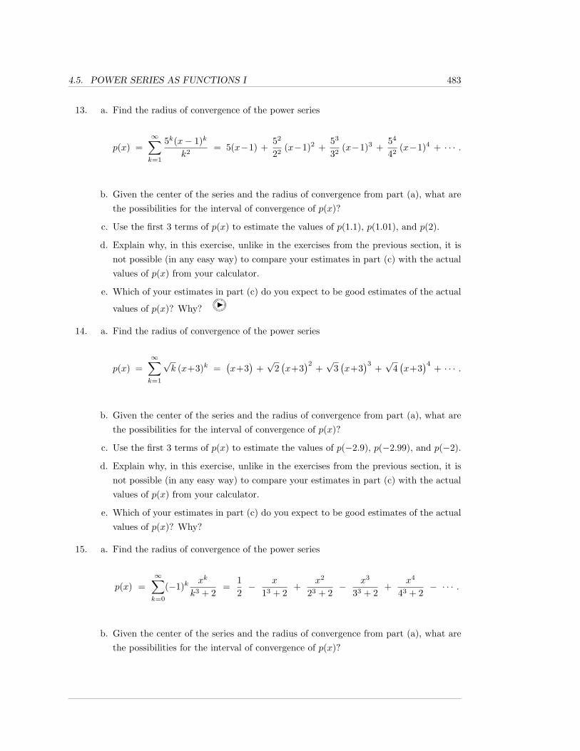
4.5. POWER SERIES AS FUNCTIONS I 483
13. a. Find the radius of convergence of the power series
p(x) =∞∑k=1
5k(x− 1)k
k2= 5(x−1) +
52
22(x−1)2 +
53
32(x−1)3 +
54
42(x−1)4 + · · · .
b. Given the center of the series and the radius of convergence from part (a), what arethe possibilities for the interval of convergence of p(x)?
c. Use the first 3 terms of p(x) to estimate the values of p(1.1), p(1.01), and p(2).
d. Explain why, in this exercise, unlike in the exercises from the previous section, it isnot possible (in any easy way) to compare your estimates in part (c) with the actualvalues of p(x) from your calculator.
e. Which of your estimates in part (c) do you expect to be good estimates of the actual
values of p(x)? Why?
14. a. Find the radius of convergence of the power series
p(x) =∞∑k=1
√k (x+3)k =
(x+3
)+√
2(x+3
)2 +√
3(x+3
)3 +√
4(x+3
)4 + · · · .
b. Given the center of the series and the radius of convergence from part (a), what arethe possibilities for the interval of convergence of p(x)?
c. Use the first 3 terms of p(x) to estimate the values of p(−2.9), p(−2.99), and p(−2).
d. Explain why, in this exercise, unlike in the exercises from the previous section, it isnot possible (in any easy way) to compare your estimates in part (c) with the actualvalues of p(x) from your calculator.
e. Which of your estimates in part (c) do you expect to be good estimates of the actualvalues of p(x)? Why?
15. a. Find the radius of convergence of the power series
p(x) =∞∑k=0
(−1)kxk
k3 + 2=
12− x
13 + 2+
x2
23 + 2− x3
33 + 2+
x4
43 + 2− · · · .
b. Given the center of the series and the radius of convergence from part (a), what arethe possibilities for the interval of convergence of p(x)?
484 CHAPTER 4. POLYNOMIALS AND POWER SERIES
c. Use the first 3 terms of p(x) to estimate the values of p(0.1), p(0.01), and p(1).
d. Explain why, in this exercise, unlike in the exercises from the previous section, it isnot possible (in any easy way) to compare your estimates in part (c) with the actualvalues of p(x) from your calculator.
e. Which of your estimates in part (c) do you expect to be good estimates of the actual
values of p(x)? Why?
16. a. Find the radius of convergence of the power series
p(x) =∞∑k=0
k!(x− 4)k
7k+1.
b. Given the center of the series and the radius of convergence from part (a), what arethe possibilities for the interval of convergence of p(x)?
c. Use the first 3 terms of p(x) to estimate the values of p(4.1), p(4.01), and p(5).
d. Explain why, in this exercise, unlike in the exercises from the previous section, it isnot possible (in any easy way) to compare your estimates in part (c) with the actualvalues of p(x) from your calculator.
e. Which of your estimates in part (c) do you expect to be good estimates of the actualvalues of p(x)? Why?
17. a. Find the radius of convergence of the power series
p(x) =∞∑k=0
(x− 4)k
7k+1.
b. Given the center of the series and the radius of convergence from part (a), what arethe possibilities for the interval of convergence of p(x)?
c. Use the first 3 terms of p(x) to estimate the values of p(4.1), p(4.01), and p(5).
d. Explain why, in this exercise, unlike in the exercises from the previous section, it isnot possible (in any easy way) to compare your estimates in part (c) with the actualvalues of p(x) from your calculator.
e. Which of your estimates in part (c) do you expect to be good estimates of the actualvalues of p(x)? Why?
4.5. POWER SERIES AS FUNCTIONS I 485
18. a. Find the radius of convergence of the power series
p(x) =∞∑k=1
(x− 4)k
7k+1k.
b. Given the center of the series and the radius of convergence from part (a), what arethe possibilities for the interval of convergence of p(x)?
c. Use the first 3 terms of p(x) to estimate the values of p(4.1), p(4.01), and p(5).
d. Explain why, in this exercise, unlike in the exercises from the previous section, it isnot possible (in any easy way) to compare your estimates in part (c) with the actualvalues of p(x) from your calculator.
e. Which of your estimates in part (c) do you expect to be good estimates of the actualvalues of p(x)? Why?
19. a. Find the radius of convergence of the power series
p(x) =∞∑k=1
(−1)k+1 (x+ 7)k
kk.
b. Given the center of the series and the radius of convergence from part (a), what arethe possibilities for the interval of convergence of p(x)?
c. Use the first 3 terms of p(x) to estimate the values of p(−6.9), p(−6.99), and p(−6).
d. Explain why, in this exercise, unlike in the exercises from the previous section, it isnot possible (in any easy way) to compare your estimates in part (c) with the actualvalues of p(x) from your calculator.
e. Which of your estimates in part (c) do you expect to be good estimates of the actualvalues of p(x)? Why?
20. a. Find the radius of convergence of the power series
p(x) =∞∑k=1
(−1)k+1 k!(x+ 7)k
kk.
b. Given the center of the series and the radius of convergence from part (a), what arethe possibilities for the interval of convergence of p(x)?
486 CHAPTER 4. POLYNOMIALS AND POWER SERIES
c. Use the first 3 terms of p(x) to estimate the values of p(−6.9), p(−6.99), and p(−6).
d. Explain why, in this exercise, unlike in the exercises from the previous section, it isnot possible (in any easy way) to compare your estimates in part (c) with the actualvalues of p(x) from your calculator.
e. Which of your estimates in part (c) do you expect to be good estimates of the actualvalues of p(x)? Why?
21. a. Find the radius of convergence of the power series
p(x) =∞∑k=1
(−1)k+1 xk
3√k.
b. Given the center of the series and the radius of convergence from part (a), what arethe possibilities for the interval of convergence of p(x)?
c. Use the first 3 terms of p(x) to estimate the values of p(0.1), p(0.01), and p(1).
d. Explain why, in this exercise, unlike in the exercises from the previous section, it isnot possible (in any easy way) to compare your estimates in part (c) with the actualvalues of p(x) from your calculator.
e. Which of your estimates in part (c) do you expect to be good estimates of the actualvalues of p(x)? Why?
22. Suppose that a power series p(x) converges at x = 1 and at x = 3, but diverges at x = −2and x = 5. What can you say about the center of the power series and the radius ofconvergence?
23. Suppose that someone tells you that they have a power series which converges at x = 1and at x = 3, but diverges at x = 2. What can you conclude?
24. In this exercise, you will show that f(x) =1
1− xis real analytic at all points a, except for
a = 1, i.e., f is real analytic on the union of open intervals (−∞, 1) ∪ (1,∞).
a. Find a formula for the k-th derivative, f (k)(x).
b. Give Lagrange’s form of the error for Ekf (x; a), where a 6= 1.
c. For each a 6= 1, find an r > 0 such that, for all x in the open interval (a − r, a + r),the limit of your error from part (b) is zero, i.e., such that 1/(1− x) = T∞f (x; a) forall x in (a− r, a+ r). (Hint: Choose r < |1− a|/2.)
d. Explain why 1/(1−x) being real analytic everywhere, except at 1, doesn’t contradictthe fact that the Maclaurin series for 1/(1− x) converges if and only if |x| < 1.
4.6. POWER SERIES AS FUNCTIONS II 487
4.6 Power Series as Functions II:Operations on Power Series
In the previous section, we discussed what it means for a power series to define a function.We looked at the interval and radius of convergence, we stated the Ratio Test, and looked atexamples of using the Ratio Test to determine radii of convergence or, in some cases, intervalsof convergence. We also discuss real analytic functions, functions which are locally equal, onopen intervals, to their Taylor series at each point.
In this section, we will look at why power series functions are so nice to deal with. We willsee that, as far as differentiation, integration, and algebraic operations are concerned, powerseries can be treated like polynomials, polynomials that just don’t ever end.
For a number of technical proofs in this section, we refer you to the excellent real analysisbook of Trench, [4].
We will begin with the following basic theorem on continuity, due to Abel.
Theorem 4.6.1. Power series functions are continuous, i.e., continuous on their intervalsof convergence, including at possible endpoints that are included in the intervals of conver-gence.
Proof. See [4], Theorem 4.5.12.
Remark 4.6.2. As we shall see below, power series functions are differentiable on the interiorof the interval of convergence, i.e., on the open interval (a − R, a + R), where a is the centerand R is the radius of convergence. As differentiable functions are continuous, the main pointof Theorem 4.6.1, for us, is that, if a power series p(x) converges at one or both of the endpointsof the interval of convergence, then the one-sided limits of p(x) as you approach the endpointequal the value of p(x) at the endpoint.
Why is this important? Suppose, for instance, that we have a function f(x) which we knowis continuous on the interval (−1, 1] and we have a power series p(x) which we know converges onthe same half-open interval (−1, 1]. Suppose, further, that we know that, on the open interval
488 CHAPTER 4. POLYNOMIALS AND POWER SERIES
(−1, 1), f(x) = p(x). Then, we can immediately conclude that, in fact, f(x) = p(x) on theentire half-open interval (−1, 1]. Why? Because Abel’s theorem, Theorem 4.6.1, tells us thatp(x) is also continuous on the interval (−1, 1], and so
f(1) = limx→1−
f(x) = limx→1−
p(x) = p(1),
where the middle inequality follows from the fact that f(x) = p(x) on the interval (−1, 1).
For example, below, we shall use integration of power series to show that, for all x in theopen interval (−1, 1),
ln(1 + x) =∞∑k=0
(−1)kxk+1
k + 1= x − x2
2+
x3
3− x4
4+
x5
5− x6
6+ · · · . (4.12)
Looking ahead to results in Chapter 5, we find that the series on the right, above, convergeswhen x = 1 and diverges when x = −1. As ln(1 + x) is continuous, and Abel’s theorem tells usthat the power series is also continuous, we conclude that
ln 2 = limx→1−
ln(1 + x) = limx→1−
[x − x2
2+
x3
3− x4
4+
x5
5− x6
6+ · · ·
]=
1 − 12
+13− 1
4+
15− 1
6+ · · · .
In other words, the equality given in Formula 4.12, which was for −1 < x < 1, also holdswhen x = 1. This provides an alternative way of showing that the alternating harmonic seriesconverges to ln 2; something we saw back in Theorem 4.4.12 and Remark 4.4.13, using Taylorerrors.
In the remainder of this section, we will sometimes assume that we have an interval I onwhich a power series converges. This does not necessarily mean that I is the entire interval ofconvergence; I could, in fact, be a smaller interval inside the interval of convergence.
We want to look now at substituting into power series. Not all substitutions lead to newpower series, but they give some infinite summation whose convergence or divergence can bediscussed.
4.6. POWER SERIES AS FUNCTIONS II 489
Example 4.6.3. Recall from Theorem 4.4.5 that we have the following equality
ex =∞∑k=0
xk
k!= 1 + x+
x2
2!+x3
3!+x4
4!+ · · · , (4.13)
for all x. Now, if x is some number, then 5(x− 1)3 is just some number, and we can stick it intoFormula 4.13 and obtain
e(5(x−1)3) = 1 + 5(x− 1)3 +
(5(x− 1)3
)22!
+
(5(x− 1)3
)33!
+
(5(x− 1)3
)44!
+ · · · =
1 + 5(x− 1)3 +25(x− 1)6
2!+
125(x− 1)9
3!+
625(x− 1)12
4!+ · · ·
Hence, we obtain a power series, centered at 1, which converges to e(5(x−1)3), for all x.
Is this series necessarily equal to the Taylor series, centered at 1, for e(5(x−1)3)? Yes, thoughwe won’t really “know” this until we have Corollary 4.6.8.
Generalizing the above example, we have:
Theorem 4.6.4. Suppose that p(x) =∑∞k=0 ck(x− a)k converges on an interval I, and we
have a second function f(x).Then, for all x such that f(x) is in I, we have the following equality
p(f(x)) =∞∑k=0
ck(f(x)− a)k,
in which the infinite sum converges.
490 CHAPTER 4. POLYNOMIALS AND POWER SERIES
In particular, if f(x) = r(x− b)m + a, where r and b are constants and m ≥ 0 is an integer,then, for all x such that r(x− b)m + a is in I, we have the following equality
p(r(x− b)m + a
)=
∞∑k=0
(ckrk)(x− b)mk,
in which the sum on the right is a convergent power series. In addition, the new interval ofconvergence consists precisely of those x values such that r(x− b)m + a is in I.
Example 4.6.5. Consider the geometric series from Theorem 4.4.10, with a = 1:
11− x
=∞∑k=0
xk = 1 + x + x2 + x3 + x4 + · · · ,
where the interval of convergence of the series, and the interval on which the equality holds, isthe open interval (−1, 1).
By substituting −3(x+ 2) in for x, we immediately obtain that
11 + 3(x+ 2)
=∞∑k=0
(− 3(x+ 2)
)k =∞∑k=0
(−1)k3k(x+ 2)k =
1 − 3(x+ 2) + +9(x+ 2)2 − 27(x+ 2)3 + 81(x+ 2)4 + · · · ,
where the equality holds, and the series converges, on precisely the interval of those x’s suchthat −3(x + 2) is in the interval (−1, 1). To determine this interval in a more standard form,you need to manipulate the inequalities
−1 < −3(x+ 2) < 1.
Divide through by −3, reversing the inequalities, to obtain
−13< x+ 2 <
13.
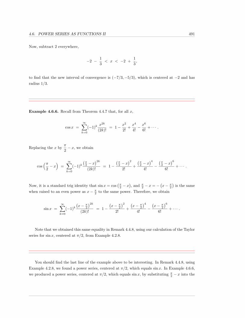
4.6. POWER SERIES AS FUNCTIONS II 491
Now, subtract 2 everywhere,
−2 − 13< x < −2 +
13,
to find that the new interval of convergence is (−7/3,−5/3), which is centered at −2 and hasradius 1/3.
Example 4.6.6. Recall from Theorem 4.4.7 that, for all x,
cosx =∞∑k=0
(−1)kx2k
(2k)!= 1− x2
2!+x4
4!− x6
6!+ · · · .
Replacing the x byπ
2− x, we obtain
cos(π
2− x)
=∞∑k=0
(−1)k(π2 − x
)2k(2k)!
= 1−(π2 − x
)22!
+
(π2 − x
)44!
−(π2 − x
)66!
+ · · · .
Now, it is a standard trig identity that sinx = cos(π2 − x
), and π
2 − x = −(x− π
2
)is the same
when raised to an even power as x− π2 to the same power. Therefore, we obtain
sinx =∞∑k=0
(−1)k(x− π
2
)2k(2k)!
= 1−(x− π
2
)22!
+
(x− π
2
)44!
−(x− π
2
)66!
+ · · · .
Note that we obtained this same equality in Remark 4.4.8, using our calculation of the Taylorseries for sinx, centered at π/2, from Example 4.2.8.
You should find the last line of the example above to be interesting. In Remark 4.4.8, usingExample 4.2.8, we found a power series, centered at π/2, which equals sinx. In Example 4.6.6,we produced a power series, centered at π/2, which equals sinx, by substituting π
2 − x into the
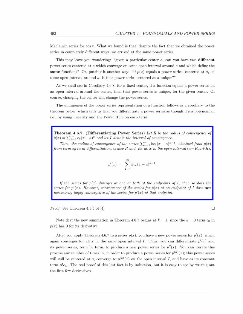
492 CHAPTER 4. POLYNOMIALS AND POWER SERIES
Maclaurin series for cosx. What we found is that, despite the fact that we obtained the powerseries in completely different ways, we arrived at the same power series.
This may leave you wondering: “given a particular center a, can you have two different
power series centered at a which converge on some open interval around a and which define thesame function?” Or, putting it another way: “if p(x) equals a power series, centered at a, onsome open interval around a, is that power series centered at a unique?”
As we shall see in Corollary 4.6.8, for a fixed center, if a function equals a power series onan open interval around the center, then that power series is unique, for the given center. Ofcourse, changing the center will change the power series.
The uniqueness of the power series representation of a function follows as a corollary to thetheorem below, which tells us that you differentiate a power series as though it’s a polynomial,i.e., by using linearity and the Power Rule on each term.
Theorem 4.6.7. (Differentiating Power Series) Let R be the radius of convergence ofp(x) =
∑∞k=0 ck(x− a)k and let I denote the interval of convergence.
Then, the radius of convergence of the series∑∞k=1 kck(x − a)k−1, obtained from p(x)
from term by term differentiation, is also R and, for all x in the open interval (a−R, a+R),
p′(x) =∞∑k=1
kck(x− a)k−1.
If the series for p(x) diverges at one or both of the endpoints of I, then so does theseries for p′(x). However, convergence of the series for p(x) at an endpoint of I does notnecessarily imply convergence of the series for p′(x) at that endpoint.
Proof. See Theorem 4.5.5 of [4].
Note that the new summation in Theorem 4.6.7 begins at k = 1, since the k = 0 term c0 inp(x) has 0 for its derivative.
After you apply Theorem 4.6.7 to a series p(x), you have a new power series for p′(x), whichagain converges for all x in the same open interval I. Thus, you can differentiate p′(x) andits power series, term by term, to produce a new power series for p′′(x). You can iterate thisprocess any number of times, n, in order to produce a power series for p(n)(x); this power serieswill still be centered at a, converge to p(n)(x) on the open interval I, and have as its constantterm n!cn. The real proof of this last fact is by induction, but it is easy to see by writing outthe first few derivatives.
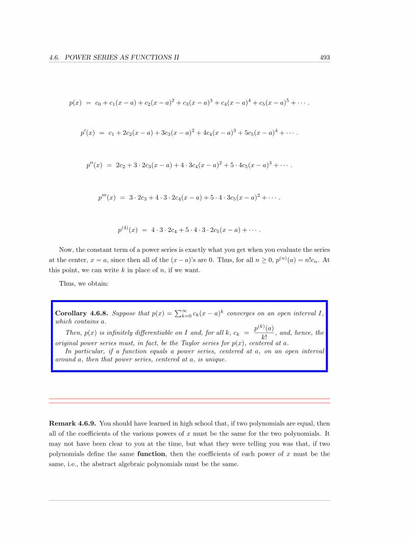
4.6. POWER SERIES AS FUNCTIONS II 493
p(x) = c0 + c1(x− a) + c2(x− a)2 + c3(x− a)3 + c4(x− a)4 + c5(x− a)5 + · · · .
p′(x) = c1 + 2c2(x− a) + 3c3(x− a)2 + 4c4(x− a)3 + 5c5(x− a)4 + · · · .
p′′(x) = 2c2 + 3 · 2c3(x− a) + 4 · 3c4(x− a)2 + 5 · 4c5(x− a)3 + · · · .
p′′′(x) = 3 · 2c3 + 4 · 3 · 2c4(x− a) + 5 · 4 · 3c5(x− a)2 + · · · .
p(4)(x) = 4 · 3 · 2c4 + 5 · 4 · 3 · 2c5(x− a) + · · · .
Now, the constant term of a power series is exactly what you get when you evaluate the seriesat the center, x = a, since then all of the (x− a)’s are 0. Thus, for all n ≥ 0, p(n)(a) = n!cn. Atthis point, we can write k in place of n, if we want.
Thus, we obtain:
Corollary 4.6.8. Suppose that p(x) =∑∞k=0 ck(x − a)k converges on an open interval I,
which contains a.
Then, p(x) is infinitely differentiable on I and, for all k, ck =p(k)(a)k!
, and, hence, the
original power series must, in fact, be the Taylor series for p(x), centered at a.In particular, if a function equals a power series, centered at a, on an open interval
around a, then that power series, centered at a, is unique.
Remark 4.6.9. You should have learned in high school that, if two polynomials are equal, thenall of the coefficients of the various powers of x must be the same for the two polynomials. Itmay not have been clear to you at the time, but what they were telling you was that, if twopolynomials define the same function, then the coefficients of each power of x must be thesame, i.e., the abstract algebraic polynomials must be the same.
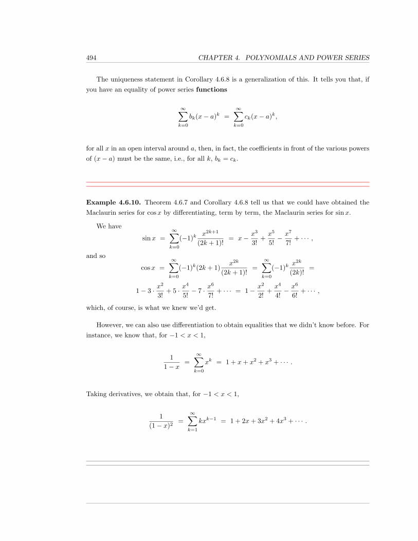
494 CHAPTER 4. POLYNOMIALS AND POWER SERIES
The uniqueness statement in Corollary 4.6.8 is a generalization of this. It tells you that, ifyou have an equality of power series functions
∞∑k=0
bk(x− a)k =∞∑k=0
ck(x− a)k,
for all x in an open interval around a, then, in fact, the coefficients in front of the various powersof (x− a) must be the same, i.e., for all k, bk = ck.
Example 4.6.10. Theorem 4.6.7 and Corollary 4.6.8 tell us that we could have obtained theMaclaurin series for cosx by differentiating, term by term, the Maclaurin series for sinx.
We have
sinx =∞∑k=0
(−1)kx2k+1
(2k + 1)!= x− x3
3!+x5
5!− x7
7!+ · · · ,
and so
cosx =∞∑k=0
(−1)k(2k + 1)x2k
(2k + 1)!=
∞∑k=0
(−1)kx2k
(2k)!=
1− 3 · x2
3!+ 5 · x
4
5!− 7 · x
6
7!+ · · · = 1− x2
2!+x4
4!− x6
6!+ · · · ,
which, of course, is what we knew we’d get.
However, we can also use differentiation to obtain equalities that we didn’t know before. Forinstance, we know that, for −1 < x < 1,
11− x
=∞∑k=0
xk = 1 + x+ x2 + x3 + · · · .
Taking derivatives, we obtain that, for −1 < x < 1,
1(1− x)2
=∞∑k=1
kxk−1 = 1 + 2x+ 3x2 + 4x3 + · · · .
4.6. POWER SERIES AS FUNCTIONS II 495
Remark 4.6.11. This is a good time to remind you of Remark 4.2.12. Suppose that f isinfinitely differentiable and defined at 0. If f is an even function, then only even-powered termsappear in the Maclaurin series of f . If f is an odd function, then only odd-powered terms appearin the Maclaurin series of f . This is true whether or not f is actually equal to its Maclaurinseries on an open interval containing 0. The proof of this was outlined for you in Exercise 37 ofSection 4.2.
You can make a stronger statement for power series functions. A power series function p(x),centered at 0, with a non-zero radius of convergence, is even (respectively, odd) if and only ifthe only terms which appear (with non-zero coefficients) in p(x) are the terms whose power iseven (respectively, odd). You are asked to show this in Exercise 39.
One slightly subtle point is that, for a function to be even or odd, for every x in the domain,it is required that −x is also in the domain. For a power series function, centered at 0, thismeans that if one endpoint of the interval of convergence I is included in I, then the otherendpoint must also be included in I. That is, for power series, centered at 0, containing onlyeven, or only odd terms, the interval of convergence is either of the form (−R,R) or [−R,R].
Example 4.6.12. Given a fixed center, the fact that power series representations of functionsare unique, and must be the Taylor series, can save you a lot of work.
Consider the function f(x) = e(x2) = ex2.
Suppose that you want to calculate the Maclaurin series of f barehandedly, i.e., from thedefinition of Maclaurin/Taylor series. To do this, you need f (k)(0), for all k, but the higher-orderderivatives of f get pretty ugly pretty fast.
f ′(x) = 2xex2,
f ′′(x) = 2(x · 2xex2
+ ex2) = 2(2x2 + 1)ex
2,
f ′′′(x) = 2[(2x2 + 1)2xex
2+ 4xex
2]= 4x(2x2 + 3)ex
2,
and so on.
However, Corollary 4.6.8 tells us that, if we can produce by any means an equality betweenex
2and a power series, centered at 0, on an open interval, then that series must be the Maclaurin
series of ex2.
496 CHAPTER 4. POLYNOMIALS AND POWER SERIES
That certainly makes things easier. By substituting x2 in for x in the Maclaurin seriesequality for ex, Theorem 4.4.5, we obtain, for all x,
ex2
=∞∑k=0
(x2)k
k!= 1 + x2 +
x4
2!+x6
3!+x8
4!+ · · · ,
for all x. Hence, this series must the Maclaurin series for ex2. Nice, huh?
Using Theorem 4.6.7 in reverse tells us how to anti-differentiate a power series functionp(x), provided that we know that the series obtained from term-by-term anti-differentiation ofthe series P (x) actually converges. Once we know how to anti-differentiate, then, since powerseries functions are continuous by Theorem 4.6.1, we can apply the Fundamental Theorem,Theorem 2.4.10, and calculate the definite integral between two points x0 and x1 in the intervalof convergence of p(x) by evaluating P (x1)− P (x0).
Theorem 4.6.13. (Integrating Power Series) Let R be the radius of convergence ofp(x) =
∑∞k=0 ck(x− a)k and let I denote the interval of convergence.
Then, for every constant C, the radius of convergence of the power series P (x) =C+
∑∞k=0
ckk+1 (x−a)k+1, obtained from p(x) from term-by-term anti-differentiation, is also
R, and, for all x in the open interval (a−R, a+R),
∫p(x) dx = C +
∞∑k=0
ckk + 1
(x− a)k+1.
If p(x) converges at one or both of the endpoints of I, then so does P (x); hence, P (x)exists and is continuous on I, making P (x) an anti-derivative of p(x) on I (Definition 2.4.5).However, divergence of p(x) at an endpoint of I does not necessarily imply divergence ofP (x) at that endpoint.
Proof. See Theorem 4.5.8 of [4].
4.6. POWER SERIES AS FUNCTIONS II 497
Remark 4.6.14. Note that, while differentiation may destroy convergence at the endpoints ofthe interval of convergence, integration can lead to convergence at the endpoints, even when theoriginal series diverged at the endpoints of the interval of convergence.
Example 4.6.15. Let’s look again at our old friend, the basic geometric series: For −1 < x < 1,
11− x
=∞∑k=0
xk = 1 + x+ x2 + x3 + · · · .
We’ll first make a substitution; we’ll replace all of the x’s with −x’s, including the x in theinequality. We obtain:
for −1 < −x < 1,
11 + x
=∞∑k=0
(−x)k =∞∑k=0
(−1)kxk = 1− x+ x2 − x3 + x4 − x5 + · · · .
Multiplying the inequality throughout by −1, and reversing the inequalities, we see that theinequality still amounts to −1 < x < 1, and so the equalities above hold on this interval.
Now, we anti-differentiate both sides of the equality to obtain that, for −1 < x < 1,
ln(1 + x) = C +∞∑k=0
(−1)kxk+1
k + 1= C + x− x2
2+x3
3− x4
4+x5
5− x6
6+ · · · ,
for some constant C.
How do you determine C? Plug in the only x value where the series is easy to evaluate: thecenter, x = 0. We find
ln(1 + 0) = C + 0 + 0 + 0 + · · · .
Therefore, C = 0, and we have, for −1 < x < 1,
ln(1 + x) =∞∑k=0
(−1)kxk+1
k + 1= x− x2
2+x3
3− x4
4+x5
5− x6
6+ · · · .
498 CHAPTER 4. POLYNOMIALS AND POWER SERIES
This is the proof of this equality for −1 < x < 0, which we stated, but didn’t prove, backin Theorem 4.4.12. Note that this proof does not instantly give you that the equality alsoholds when x = 1, though our Taylor error proof in Theorem 4.4.12 did give us the equalityat x = 1. If we ignore our earlier proof of the convergence of the alternating harmonic seriesand, instead, use another result (like the Alternating Series Test, Theorem 5.4.17 to show thatthe alternating harmonic series converges, we can obtain the x = 1 equality by using Abel’stheorem on continuity, as we discussed in Remark 4.6.2.
Note that integration changed divergence at x = 1 in the original series into convergence atx = 1 for the integrated series. Of course, this means that term-by-term differentiation of theMaclaurin series for ln(1 + x) destroys convergence at x = 1.
Example 4.6.16. Let’s start from one of our series equalities from the last example:
for −1 < x < 1,
11 + x
=∞∑k=0
(−1)kxk = 1− x+ x2 − x3 + x4 − x5 + · · · .
This time, we substitute x2 in for x to obtain:
for −1 < x2 < 1,
11 + x2
=∞∑k=0
(−1)kx2k = 1− x2 + x4 − x6 + x8 − x10 + · · · . (4.14)
The condition that −1 < x2 < 1 once again is equivalent to −1 < x < 1, and so we have theabove equalities for all x in the open interval (−1, 1).
Now, recalling that (tan−1 x)′ = 1/(1 + x2), let’s anti-differentiate the equality in For-mula 4.14 to obtain
tan−1 x = C +∞∑k=0
(−1)kx2k+1
2k + 1= C + x− x3
3+x5
5− x7
7+x9
9− x11
11+ · · · .
Once again, plug in the x value of the center of the series to determine C. We find that
4.6. POWER SERIES AS FUNCTIONS II 499
C = tan−1(0) = 0, and so, we arrive at
tan−1 x =∞∑k=0
(−1)kx2k+1
2k + 1= x− x3
3+x5
5− x7
7+x9
9− x11
11+ · · · , (4.15)
for −1 < x < 1.
Of course, tan−1 x is continuous, and so, using Abel’s theorem again, we can conclude thatthis last equality holds at x = ±1, provided that we know that the series actually convergesat x = ±1. In fact, the same Alternating Series Test, Theorem 5.4.17, that tells us thatthe alternating harmonic series converges also tells us quickly that the series in Formula 4.15converges at both x = ±1, and so the equality in Formula 4.15 holds for all x in the closedinterval [−1, 1].
One cool “application” of this is that it implies that
π
4= tan−1(1) =
∞∑k=0
(−1)k1
2k + 1= 1− 1
3+
15− 1
7+
19− 1
11+ · · · .
Hence,
π = 4(
1− 13
+15− 1
7+
19− 1
11+ · · ·
),
and we could use this to approximate π by using partial sums to estimate the infinite sum. Thisis actually not a very efficient method for approximating π. For instance, we find
π ≈ 4(
1− 13
+15− 1
7+
19− 1
11+
113− 1
15+
117− 1
19
)“ = ” 3.041839618929,
which is not very close to 3.141592653590. To get reasonable accuracy, you would have to use apartial sum with many, many terms.
We now need to discuss algebraic operations with power series. What we shall see is that youadd, subtract, multiply, and divide power series as though they are never-ending polynomials.However, the precise manner in which you deal with multiplication and division requires somediscussion.
500 CHAPTER 4. POLYNOMIALS AND POWER SERIES
Theorem 4.6.17. Suppose that p(x) =∑∞k=0 ck(x − a)k and q(x) =
∑∞k=0 dk(x − a)k
converge on an interval I.Then, for all x in I, we have the following equality of functions:
p(x) + q(x) =∞∑k=0
(ck + dk)(x− a)k,
where, in particular, we mean that the series converges for all x in I.
In words, we say that summations of two power series with the same center is performed“term-wise”.
Proof. This follows at once from the analogous theorem for series of constants, Theorem 5.2.17,which is left to you as an easy exercise in Section 5.2.
The following theorem basically says that multiplication distributes over addition, even ifthe addition is of an infinite number of things. It follows at once from distributing in the partialsums, and using basic limit properties.
Theorem 4.6.18. Suppose that p(x) =∑∞k=0 ck(x − a)k converges on an interval I, and
that f(x) is a function defined on I.Then, for all x in I,
∑∞k=0 f(x)ck(x− a)k converges, and
f(x)p(x) =∞∑k=0
f(x)ck(x− a)k.
In particular, if f(x) = r(x− a)m, where r is a constant and m ≥ 0 is an integer, then we
obtain that r(x− a)mp(x) equals the power series∞∑k=0
rck(x− a)k+m.
4.6. POWER SERIES AS FUNCTIONS II 501
Example 4.6.19. Of course, you can combine Theorem 4.6.17 and Theorem 4.6.18 to findpower series representations of various combinations of known series. For instance, for all x,
5 sinx+ 3x cosx = 5∞∑k=0
x2k+1
(2k + 1)!+ 3x
∞∑k=0
x2k
(2k)!=
∞∑k=0
[5
(2k + 1)!+
3(2k)!
]x2k+1 =
8x +(
53!
+32!
)x3 +
(55!
+34!
)x5 +
(57!
+36!
)x7 + · · · .
Note that, as we discussed in Remark 4.6.11, the odd function 5 sinx+3x cosx has a Maclau-rin series contained only odd-powered terms.
Example 4.6.20. Power series manipulations can help you calculate limits.
For instance, for all x 6= 0,
ex − 1− xx2
=1x2·[(−1− x) + 1 + x+
x2
2!+x3
3!+x4
4!+ · · ·
]=
1x2·[x2
2!+x3
3!+x4
4!· · ·]
=12!
+x
3!+x2
4!+ · · ·
Therefore, as power series are continuous, we find that
limx→0
ex − 1− xx2
= limx→0
(12!
+x
3!+x2
4!+ · · ·
)=
12!
+ 0 + 0 + · · · =12.
Example 4.6.21. In this example, we “cheat” and must use that Calculus and the theory ofinfinite series work perfectly well when you use complex numbers in place of real numbers. Thismeans that, in this example, we want to allow numbers of the form a + bi, where a and b arereal numbers, and i is a square root of −1, i.e., i2 = −1.
Note that, when you look at positive integral powers of i, what you get repeats every foursteps:
i1 = i, i2 = −1, i3 = i2 · i = −i, i4 = (−1)i2 = (−1)(−1) = 1,
502 CHAPTER 4. POLYNOMIALS AND POWER SERIES
i5 = i · i4 = i · 1 = i, i6 = i2 · i4 = i2 · 1 = i2 = −1, etc.
Now, let’s replace the x in
ex = 1 + x+x2
2!+x3
3!+x4
4!+x5
5!+x6
6!+x7
7!+ · · ·
by iθ, where we’re thinking of θ being a real number (but it doesn’t have to be). In fact, we’rethinking of θ as an angle (hence, the use of variable θ); we shall see why in minute. Using whatwe wrote about how the powers of i work, we obtain
eiθ = 1 + iθ +i2θ2
2!+i3θ3
3!+i4θ4
4!+i5θ5
5!+i6θ6
6!+i7θ7
7!+ · · · =
1 + iθ − θ2
2!− i θ
3
3!+θ4
4!+ i
θ5
5!− θ6
6!− i θ
7
7!+ · · · =
(1− θ2
2!+θ4
4!− θ6
6!+ · · ·
)+ i
(θ − θ3
3!+θ5
5!− θ7
7!+ · · ·
)=
cos θ + i sin θ.
This fundamental result, that
eiθ = cos θ + i sin θ (4.16)
is of great importance in many areas of mathematics, physics, and electrical engineering; thisequality is known as Euler’s Formula.
As a quick example of the usefulness of Euler’s Formula, let’s see how easily it lets youderive the angle addition formulas for sine and cosine. We will use that, if a, b, c and d are realnumbers, then a+ bi = c+ di if and only if a = c and b = d.
Suppose that α and β are real numbers. Euler’s Formula tells us that
eiα = cosα + i sinα and eiβ = cosβ + i sinβ.
4.6. POWER SERIES AS FUNCTIONS II 503
Multiplying, we obtain
eiα · eiβ = cosα cosβ + i2 sinα sinβ + i cosβ sinα+ i cosα sinβ,
and soei(α+β) =
(cosα cosβ − sinα sinβ
)+ i(
cosβ sinα+ cosα sinβ).
Applying Euler’s Formula one more time to ei(α+β), we find that
cos(α+ β) + i sin(α+ β) =(
cosα cosβ − sinα sinβ)
+ i(
cosβ sinα+ cosα sinβ)
and, therefore, matching the parts without the i’s (the real parts) and the parts with the i’s (theimaginary parts), we obtain the well-known angle addition formulas:
cos(α+ β) = cosα cosβ − sinα sinβ
andsin(α+ β) = cosβ sinα+ cosα sinβ.
So cool.
Example 4.6.22. Now that we have Euler’s Formula, we can also give the close relationshipbetween hyperbolic sine and cosine, from Definition 1.4.1, and the usual, circular, sine andcosine.
Euler’s Formula tells us that eiθ = cos θ+ i sin θ. Replacing θ with −θ, and using that cosineis an even function and sine is an odd function, we find that e−iθ = cos θ − i sin θ.
Therefore, we obtain
cosh(iθ) =eiθ + e−iθ
2=
cos θ + i sin θ + cos θ − i sin θ2
= cos θ
and
sinh(iθ) =eiθ − e−iθ
2=
cos θ + i sin θ − cos θ + i sin θ2
= i sin θ.
504 CHAPTER 4. POLYNOMIALS AND POWER SERIES
Or, replacing θ with −iθ, and using i2 = −1 and the even- and odd-ness of cosine and sine,we have
cosh θ = cos(iθ) and sinh θ = −i sin(iθ).
There are still three important operations with power series that we want to look at: multi-plying two power series with the same center, dividing two power series with the same center,and composing power series, which, in fact, is best discussed in terms of real analytic functions(Definition 4.5.20).
Example 4.6.23. Consider the two polynomials, centered at a:
p(x) = b0 +b1(x−a)+b2(x−a)2 +b3(x−a)3 and q(x) = c0 +c1(x−a)+c2(x−a)2 +c3(x−a)3.
Multiplying p(x) times q(x), and collecting powers of (x− a), you find
p(x) · q(x) = b0c0 + (b0c1 + b1c0)(x− a) + (b0c2 + b1c1 + b2c0)(x− a)2 +
(b0c3 + b1c2 + b2c1 + b3c0)(x− a)3 + higher-degree terms
You shouldn’t memorize this, but hopefully you see the pattern: the coefficient in front of the(x− a)n term in the product is a sum of the products of coefficients of the two individual powerseries, and the indices of the coefficients from p(x) and q(x) always add up to n, the exponentof (x − a)n. It is not hard to understand why this is true: to obtain an (x − a)n term in theproduct, you can take any term from p(x) of degree k, where 0 ≤ k ≤ n, and multiply it bya term from q(x) of degree n − k, i.e., take bk(x − a)j · cn−k(x − a)n−k = bkcn−k(x − a)n. Ofcourse, you get a summand of this form for each k such that 0 ≤ k ≤ n.
This pattern actually continues where we have written “higher-degree terms”; it’s just thatmany of the coefficients involved in the terms of degree ≥ 4 are zero, since those terms are zero(i.e., don’t appear) in p(x) and q(x).
The same process that we used in the above example applies to infinite series.
4.6. POWER SERIES AS FUNCTIONS II 505
Theorem 4.6.24. Suppose that p(x) =∑∞k=0 bk(x − a)k and q(x) =
∑∞k=0 ck(x − a)k
converge on an open interval I.Then, for all x in I, we have the following equality of functions:
p(x) · q(x) =∞∑n=0
(n∑k=0
bkcn−k
)(x− a)n,
where, in particular, we mean that the series converges for all x in I.
Proof. This follows from Theorem 5.4.11, combined with the fact that power series convergeabsolutely on the interior of the interval of convergence; see Theorem 4.5.9.
Example 4.6.25. Find the 5th order Maclaurin polynomial of ex sinx, and use it to approxi-mate e0.1 sin(0.1).
Solution:
We could do this “simply” by calculating the 5th order Maclaurin polynomial from thedefinition, Definition 4.2.2. However, instead, we will use Theorem 4.6.24 and just do themultiplication out to the degree 5 term.
We haveex = 1 + x+
x2
2!+x3
3!+x4
4!+x5
5!+ · · ·
andsinx = x− x3
3!+x5
5!− · · · .
Don’t get confused by the missing terms in the sinx series; if it helps, explicitly insert zerotimes each of the even powers of x. However, you shouldn’t really have to write those terms in –just keep in mind that they’re there or, equivalently, that when a term is missing, you don’t getthe corresponding product. Think: How do you get a degree 0 term in the product? You haveto multiply a degree 0 term from ex times a degree 0 term from sinx; but there is no degree0 term in the sinx series, so you don’t get a degree 0 term in the product. How do you get adegree 1 term in the product? By multiplying a degree 0 term from ex times a degree 1 termfrom sinx – yielding 1 ·x – and/or by multiplying a degree 1 term from ex times a degree 0 termfrom sinx – but this portion doesn’t appear since there is no degree 0 term from sinx. Justcontinue in this manner.
506 CHAPTER 4. POLYNOMIALS AND POWER SERIES
What you should find is (we’ve included the 0’s, in case you thought of it like that):
ex sinx = 0 + (1 + 0)x+ (0 + 1 + 0)x2 +(− 1
3!+ 0 +
12!
+ 0)x3 +
(0− 1
3!+ 0 +
13!
+ 0)x4+
(15!
+ 0− 12!· 1
3!+ 0 +
14!
+ 0)x5 + · · · .
Simplifying, we find that the 5th order Maclaurin polynomial of ex sinx is
x+ x2 +13x3 − 1
30x5.
As 0.1 is reasonably close to the center 0, we expect that a decent approximation of e0.1 sin(0.1)is given by
0.1 + (0.1)2 +13
(0.1)3 − 130
(0.1)5 = 0.110333.
The calculator value of e0.1 sin(0.1) is 0.110332988730, so our approximation looks very good.
Now let’s look at division.
Example 4.6.26. Knowing the Maclaurin series for ex, sinx, and cosx, can we determineMaclaurin series or, at least, the 4th order Maclaurin polynomials, for ex/ sinx and ex/ cosx inan algebraic manner, rather than by taking lots of fairly ugly derivatives?
For ex/ sinx, the answer is certainly no; you can’t have a Maclaurin series for this functionbecause the function itself is undefined at x = 0. More generally, if you have two power seriescentered at a, p(x) and q(x), and you want a power series centered at a which equals p(x)/q(x),you at least need q(a) 6= 0, i.e., if q(x) =
∑∞k=0 ck(x− a)k, you need c0 6= 0.
So, what about ex/ cosx? Can we long divide one series into another to find
1 + x+x2
2!+x3
3!+x4
4!+x5
5!+ · · ·
1− x2
2!+x4
4!− x6
6!+ · · ·
= d0 + d1x+ d2x2 + d3x
3 + d4x4 + · · · ?
The answer is that, yes, we could describe long division, but it’s actually nicer to work backwardsfrom the multiplication. That is, we’re going to solve for the coefficients dk that make the
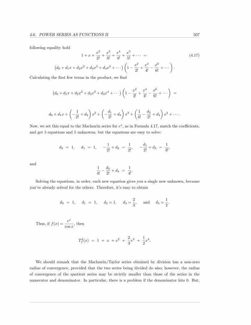
4.6. POWER SERIES AS FUNCTIONS II 507
following equality hold
1 + x+x2
2!+x3
3!+x4
4!+x5
5!+ · · · = (4.17)
(d0 + d1x+ d2x
2 + d3x3 + d4x
4 + · · ·)(
1− x2
2!+x4
4!− x6
6!+ · · ·
).
Calculating the first few terms in the product, we find
(d0 + d1x+ d2x
2 + d3x3 + d4x
4 + · · ·)(
1− x2
2!+x4
4!− x6
6!+ · · ·
)=
d0 + d1x+(− 1
2!+ d2
)x2 +
(−d1
2!+ d3
)x3 +
(14!− d2
2!+ d4
)x4 + · · · .
Now, we set this equal to the Maclaurin series for ex, as in Formula 4.17, match the coefficients,and get 5 equations and 5 unknowns, but the equations are easy to solve:
d0 = 1, d1 = 1, − 12!
+ d2 =12!, −d1
2!+ d3 =
13!,
and14!− d2
2!+ d4 =
14!.
Solving the equations, in order, each new equation gives you a single new unknown, becauseyou’ve already solved for the others. Therefore, it’s easy to obtain
d0 = 1, d1 = 1, d2 = 1, d3 =23, and d4 =
12.
Thus, if f(x) =ex
cosx, then
T 4f (x) = 1 + x + x2 +
23x3 +
12x4.
We should remark that the Maclaurin/Taylor series obtained by division has a non-zeroradius of convergence, provided that the two series being divided do also; however, the radiusof convergence of the quotient series may be strictly smaller than those of the series in thenumerator and denominator. In particular, there is a problem if the denominator hits 0. But,
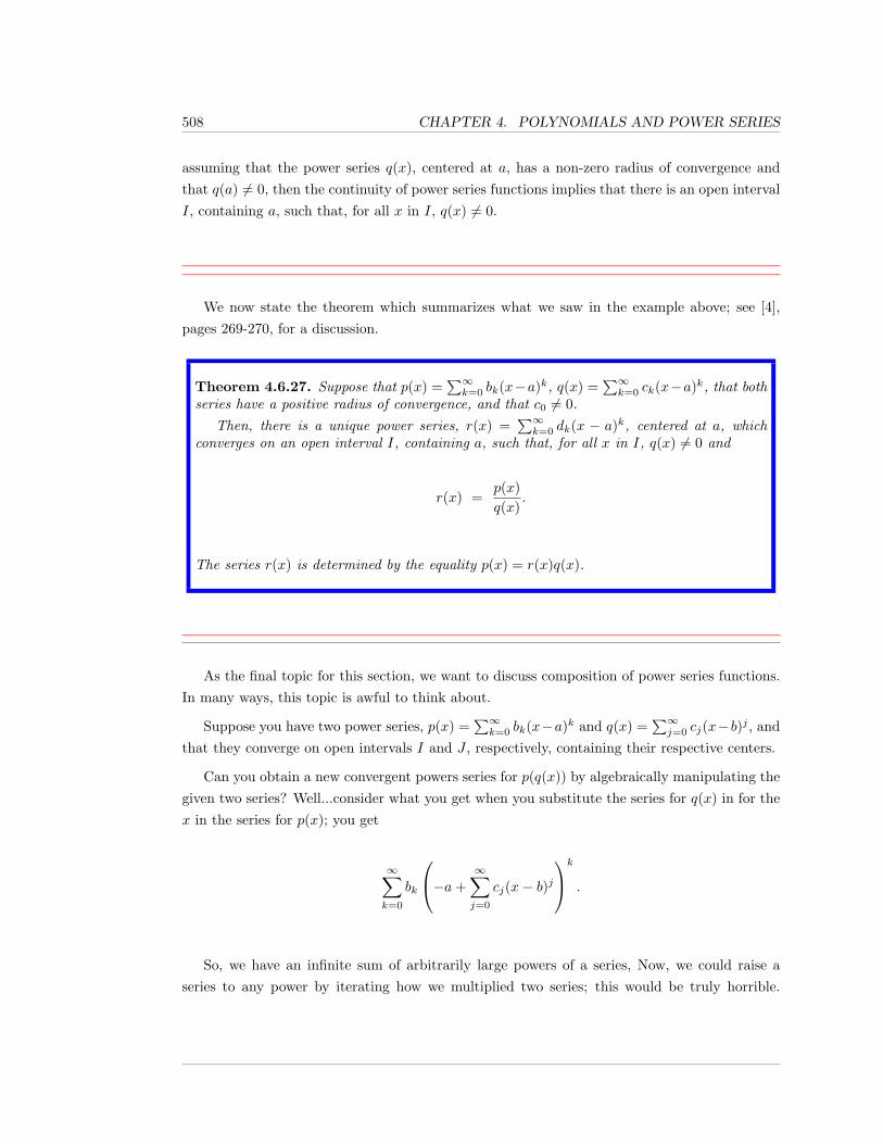
508 CHAPTER 4. POLYNOMIALS AND POWER SERIES
assuming that the power series q(x), centered at a, has a non-zero radius of convergence andthat q(a) 6= 0, then the continuity of power series functions implies that there is an open intervalI, containing a, such that, for all x in I, q(x) 6= 0.
We now state the theorem which summarizes what we saw in the example above; see [4],pages 269-270, for a discussion.
Theorem 4.6.27. Suppose that p(x) =∑∞k=0 bk(x−a)k, q(x) =
∑∞k=0 ck(x−a)k, that both
series have a positive radius of convergence, and that c0 6= 0.Then, there is a unique power series, r(x) =
∑∞k=0 dk(x − a)k, centered at a, which
converges on an open interval I, containing a, such that, for all x in I, q(x) 6= 0 and
r(x) =p(x)q(x)
.
The series r(x) is determined by the equality p(x) = r(x)q(x).
As the final topic for this section, we want to discuss composition of power series functions.In many ways, this topic is awful to think about.
Suppose you have two power series, p(x) =∑∞k=0 bk(x−a)k and q(x) =
∑∞j=0 cj(x−b)j , and
that they converge on open intervals I and J , respectively, containing their respective centers.
Can you obtain a new convergent powers series for p(q(x)) by algebraically manipulating thegiven two series? Well...consider what you get when you substitute the series for q(x) in for thex in the series for p(x); you get
∞∑k=0
bk
−a+∞∑j=0
cj(x− b)jk
.
So, we have an infinite sum of arbitrarily large powers of a series, Now, we could raise aseries to any power by iterating how we multiplied two series; this would be truly horrible.
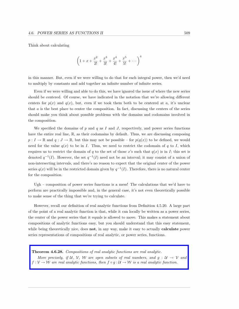
4.6. POWER SERIES AS FUNCTIONS II 509
Think about calculating
(1 + x+
x2
2!+x3
3!+x4
4!+x5
5!+ · · ·
)4
in this manner. But, even if we were willing to do that for each integral power, then we’d needto multiply by constants and add together an infinite number of infinite series.
Even if we were willing and able to do this, we have ignored the issue of where the new seriesshould be centered. Of course, we have indicated in the notation that we’re allowing differentcenters for p(x) and q(x), but, even if we took them both to be centered at a, it’s unclearthat a is the best place to center the composition. In fact, discussing the centers of the seriesshould make you think about possible problems with the domains and codomains involved inthe composition.
We specified the domains of p and q as I and J , respectively, and power series functionshave the entire real line, R, as their codomains by default. Thus, we are discussing composingp : I → R and q : J → R, but this may not be possible – for p(q(x)) to be defined, we wouldneed for the value q(x) to be in I. Thus, we need to restrict the codomain of q to I, whichrequires us to restrict the domain of q to the set of those x’s such that q(x) is in I; this set isdenoted q−1(I). However, the set q−1(I) need not be an interval; it may consist of a union ofnon-intersecting intervals, and there’s no reason to expect that the original center of the powerseries q(x) will be in the restricted domain given by q−1(I). Therefore, there is no natural centerfor the composition.
Ugh – composition of power series functions is a mess! The calculations that we’d have toperform are practically impossible and, in the general case, it’s not even theoretically possibleto make sense of the thing that we’re trying to calculate.
However, recall our definition of real analytic functions from Definition 4.5.20. A large partof the point of a real analytic function is that, while it can locally be written as a power series,the center of the power series that it equals is allowed to move. This makes a statement aboutcompositions of analytic functions easy, but you should understand that this easy statement,while being theoretically nice, does not, in any way, make it easy to actually calculate powerseries representations of compositions of real analytic, or power series, functions.
Theorem 4.6.28. Compositions of real analytic functions are real analytic.More precisely, if U , V, W are open subsets of real numbers, and g : U → V and
f : V → W are real analytic functions, then f ◦ g : U → W is a real analytic function.
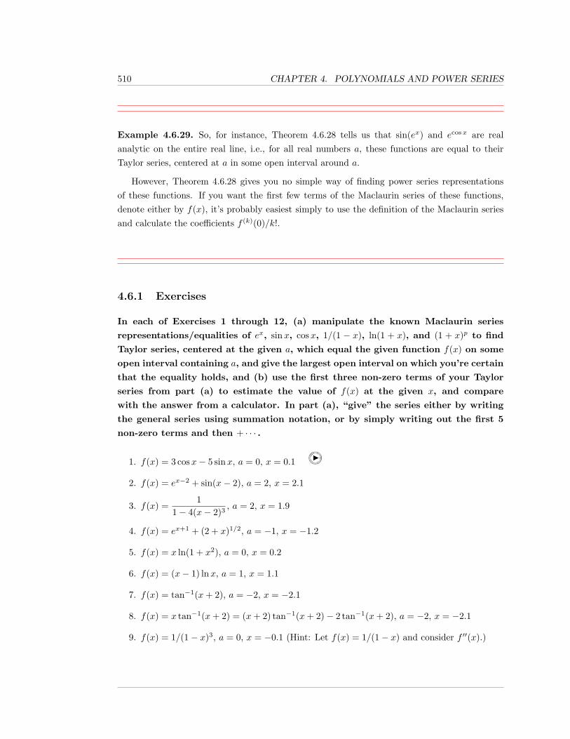
510 CHAPTER 4. POLYNOMIALS AND POWER SERIES
Example 4.6.29. So, for instance, Theorem 4.6.28 tells us that sin(ex) and ecos x are realanalytic on the entire real line, i.e., for all real numbers a, these functions are equal to theirTaylor series, centered at a in some open interval around a.
However, Theorem 4.6.28 gives you no simple way of finding power series representationsof these functions. If you want the first few terms of the Maclaurin series of these functions,denote either by f(x), it’s probably easiest simply to use the definition of the Maclaurin seriesand calculate the coefficients f (k)(0)/k!.
4.6.1 Exercises
In each of Exercises 1 through 12, (a) manipulate the known Maclaurin series
representations/equalities of ex, sinx, cosx, 1/(1 − x), ln(1 + x), and (1 + x)p to find
Taylor series, centered at the given a, which equal the given function f(x) on some
open interval containing a, and give the largest open interval on which you’re certain
that the equality holds, and (b) use the first three non-zero terms of your Taylor
series from part (a) to estimate the value of f(x) at the given x, and compare
with the answer from a calculator. In part (a), “give” the series either by writing
the general series using summation notation, or by simply writing out the first 5
non-zero terms and then + · · · .
1. f(x) = 3 cosx− 5 sinx, a = 0, x = 0.1
2. f(x) = ex−2 + sin(x− 2), a = 2, x = 2.1
3. f(x) =1
1− 4(x− 2)3, a = 2, x = 1.9
4. f(x) = ex+1 + (2 + x)1/2, a = −1, x = −1.2
5. f(x) = x ln(1 + x2), a = 0, x = 0.2
6. f(x) = (x− 1) lnx, a = 1, x = 1.1
7. f(x) = tan−1(x+ 2), a = −2, x = −2.1
8. f(x) = x tan−1(x+ 2) = (x+ 2) tan−1(x+ 2)− 2 tan−1(x+ 2), a = −2, x = −2.1
9. f(x) = 1/(1− x)3, a = 0, x = −0.1 (Hint: Let f(x) = 1/(1− x) and consider f ′′(x).)
4.6. POWER SERIES AS FUNCTIONS II 511
10. f(x) = 3√
8 + x3, a = 0, x = 0.1
11. f(x) = cos(√x− 4), a = 4, x = 4.01
12. f(x) =∫ x
0
t2√1 + t2
dt, a = 0, x = 0.1
In each of Exercises 13 through 21, differentiate and anti-differentiate the given
series, giving the result in summation notation (preceded by a big C+ for the anti-
derivative) and writing out the first 5 (not counting the C+) non-zero terms of the
summations. Give the center and radius of convergence of the original series, and
of the derivative and anti-derivative series; note that the given series are those from
Exercises 13 through 21 of Section 4.5.
13. p(x) =∞∑k=1
5k(x− 1)k
k2= 5(x− 1) +
52
22(x− 1)2 +
53
32(x− 1)3 +
54
42(x− 1)4 + · · · .
14. p(x) =∞∑k=1
√k (x+ 3)k =
(x+ 3
)+√
2(x+ 3
)2 +√
3(x+ 3
)3 +√
4(x+ 3
)4 + · · · .
15. p(x) =∞∑k=0
(−1)kxk
k3 + 2=
12− x
13 + 2+
x2
23 + 2− x3
33 + 2+
x4
43 + 2− · · · .
16. p(x) =∞∑k=0
k!(x− 4)k
7k+1.
17. p(x) =∞∑k=0
(x− 4)k
7k+1.
18. p(x) =∞∑k=1
(x− 4)k
7k+1k.
19. p(x) =∞∑k=1
(−1)k+1 (x+ 7)k
kk.
20. p(x) =∞∑k=1
(−1)k+1 k!(x+ 7)k
kk.
21. p(x) =∞∑k=1
(−1)k+1 xk
3√k.
In each of Exercises 21 through 26, write out the first 5 non-zero terms of the
product of the two given series, using the same (common) center as the given
series.
512 CHAPTER 4. POLYNOMIALS AND POWER SERIES
22. p(x) =∞∑k=0
2k(x− 1)k
k!and q(x) =
∞∑k=0
(−1)k(x− 1)k
k!
23. p(x) =∞∑k=0
(−1)kxk+1
k + 1and q(x) =
∞∑k=0
xk
24. p(x) =∞∑k=0
(−1)kx2k+1
(2k + 1)!and q(x) =
∞∑k=0
xk
25. p(x) =∞∑k=0
(−1)kx2k
(2k)!and q(x) =
∞∑k=0
xk
26. p(x) =∞∑k=1
(−1)k+1 (x− 3)k√k
and q(x) = p(x) =∞∑k=1
(−1)k+1 (x− 3)k√k
27. p(x) =∞∑k=1
(−1)k+1 (x− 3)k√k
and q(x) =∞∑k=0
(x− 3)k
k!
28. Multiply the Maclaurin series for sinx and cosx together, and write out the first 5 non-zero terms. You should get the Maclaurin series for a sin(bx), for some constants a and b.What are a and b?
In each of Exercises 27 through 32, write out the first 4 non-zero terms of p(x)/q(x),using the same (common) center as the given series.
29. p(x) =∞∑k=0
2k(x− 1)k
k!and q(x) =
∞∑k=0
(−1)k(x− 1)k
k!
30. p(x) =∞∑k=0
(−1)kxk+1
k + 1and q(x) =
∞∑k=0
xk
31. p(x) =∞∑k=0
(−1)kx2k+1
(2k + 1)!and q(x) =
∞∑k=0
xk
32. p(x) =∞∑k=0
(−1)kx2k
(2k)!and q(x) =
∞∑k=0
xk
33. p(x) = 1 +∞∑k=1
(−1)k+1 (x− 3)k√k
and q(x) = p(x) = 1 +∞∑k=1
(−1)k+1 (x− 3)k√k
34. p(x) =∞∑k=1
(−1)k+1 (x− 3)k√k
and q(x) =∞∑k=0
(x− 3)k
k!
4.6. POWER SERIES AS FUNCTIONS II 513
35. What quadratic polynomial best approximates cos(√x), when x is close to 0?
36. What cubic polynomial best approximates tan−1(x+ 5), when x is close to −5?
37. What polynomial of degree 5 best approximates x ln(1 +x2), when x is close to 0?
38. What polynomial of degree 4 best approximates e(x−1)2 , when x is close to 1?
39. In this exercise, you are asked to prove the statements made in Remark 4.6.11
a. Suppose that a power series, centered at 0, with radius of convergence R, has onlyeven-powered terms or only odd-powered terms. Prove that the interval of conver-gence is either (−R,R) or [−R,R].
b. Prove that a power series function p(x), centered at 0, with a non-zero radius ofconvergence, is even (respectively, odd) if and only if the only terms which appear(with non-zero coefficients) in p(x) are the terms whose power is even (respectively,odd).
40. Recall Remark 1.1.23: the function f(x) = e−x2
has no elementary anti-derivative. How-ever, elementary functions involve finite combinations of certain basic functions, andpower series are infinite sums.
a. Find a power series anti-derivative of e−x2.
b. Use the 3rd order Maclaurin polynomial from your answer in part a) to approximate∫ 1
0e−x
2dx.
41. The function f(x) = cos(x2) has no elementary anti-derivative, but we can find a powerseries anti-derivative.
a. Find a power series anti-derivative of cos(x2).
b. Use the 3rd order Maclaurin polynomial from your answer in part a) to approximate∫ 1
0cos(x2) dx.
42. The function f(x) = sin(x2) has no elementary anti-derivative, but we can find a power
series anti-derivative.
a. Find a power series anti-derivative of sin(x2).
b. Use the 3rd order Maclaurin polynomial from your answer in part a) to approximate∫ 1
0sin(x2) dx.
43. In this exercise, we lead you through the steps of proving the Binomial Theorem, Theo-
rem 4.4.14. Recall that(p
0
)= 1 and, for k ≥ 1,
(p
k
)= p(p− 1)(p− 2) · · · (p−k+ 1)/(k!).
514 CHAPTER 4. POLYNOMIALS AND POWER SERIES
a. Let
f(x) =∞∑k=0
(p
k
)xk.
Use the Ratio Test to show that f(x) converges (absolutely) for |x| < 1.
b. Calculate the Maclaurin series for f ′(x).
c. Show that, for |x| < 1,(1 + x)f ′(x) = p f(x).
d. Solve the separable differential equation in the last part, and use the initial data thatf(0) = 1, to show that, for |x| < 1, f(x) = (1 + x)p.
44. Square both sides of Euler’s Formula, Formula 4.16, eiθ = cos θ + i sin θ. What well-known identities, using only real numbers, do you obtain for sin(2θ) and cos(2θ)?
45. Cube both sides of Euler’s Formula, Formula 4.16, eiθ = cos θ + i sin θ. What not-so-well-known identities, using only real numbers, do you obtain for sin(3θ) and cos(3θ)?
4.7. POWER SERIES SOLUTIONS 515
4.7 Power Series Solutionsof Differential Equations
One important application of power series functions is using them to find solutions to differentialequations and/or initial value problems (IVP’s). We discussed differential equations and IVP’sat length in the final chapter of [2], before we had power series at our disposal.
How do power series help you solve differential equations and/or IVP’s? You assume thatthere is a power series solution to the differential equation, centered at the x-coordinate of theinitial data in the case of an IVP. You then plug in a power series with unknown coefficients,and this frequently leads to a manageable, but infinite, set of simultaneous equations to solve,or from which to derive a general formula for the coefficients. Your solution is then the powerseries that you end up with, or an approximate solution is given by using the first few non-zeroterms.
Sometimes, you may recognize your power series solution as being equal to some combinationof standard functions, i.e., you may recognize it as an elementary function when you’re finished,but this is not something to be expected in general.
Example 4.7.1. Let’s begin with a separable differential equation, one that we can solveexplicitly, so that we can compare with the power series solution.
Consider the IVP:dy
dx= xy; y(0) = 5.
The differential equation is separable. We find
∫1ydy =
∫x dx.
Thus, ln |y| = x2/2 + C and, after some algebra, we find y = Aex2/2, for some constant A.
Plugging in the initial data, we find that A = 5, so that the unique solution to the IVP is
y = 5ex2/2.
Okay. So, how does the power series approach go?
516 CHAPTER 4. POLYNOMIALS AND POWER SERIES
We look for a power series solution to the IVP. Since the x value of the initial data is 0, welook for a power series centered at 0. Thus, we want to find the coefficients b0, b1, b2, . . . sothat
y = y(x) =∞∑k=0
bkxk = b0 + b1x+ b2x
2 + b3x3 + · · ·
is a solution to the IVP.
First of all, we immediately know that we need b0 = 5, because we have
5 = y(0) = b0 + 0 + 0 + 0 + · · · = b0.
To find the rest of the bk, we take our power series expression for y, and the differentialequation
y′ = xy
becomes an equality of power series functions, centered at 0. As power series functions areunique, by Corollary 4.6.8, and as we discussed in Remark 4.6.9, we can match coefficients onboth sides of the equation, and solve for the bk’s. The only slight difficulty is in re-indexing thesummations, but we’ll get to that in a minute.
Since
y(x) =∞∑k=0
bkxk,
we use the Power Rule, term-by term, and find
y′ =∞∑k=1
kbkxk−1.
If we want our index to be the power of x (as usual), then, as an intermediate step, let j = k−1,so that k = j + 1. As k goes from 1 to ∞, j will go from 0 to ∞, and so
y′ =∞∑k=1
kbkxk−1 =
∞∑j=0
(j + 1)bj+1xj . (4.18)
Now,
xy = x ·∞∑k=0
bkxk =
∞∑k=0
bkxk+1,
4.7. POWER SERIES SOLUTIONS 517
and, once again, if we want to index by the power of x, we let j = k+ 1, so that k = j − 1, andthis time we find
xy =∞∑j=1
bj−1xj .
Combining this last equation with Formula 4.18, we find that our differential equation givesus
∞∑j=0
(j + 1)bj+1xj =
∞∑j=1
bj−1xj .
We would like to say, at this point, that we now match the coefficients of the powers of x onboth sides of the equation. However, one summation starts at j = 0 and the other starts atj = 1. But this is no real problem; we simply split off the j = 0 term, and write
b1 +∞∑j=1
(j + 1)bj+1xj =
∞∑j=1
bj−1xj .
Now we can match coefficients. The constant term on the left is b1 and there is no constantterm on the right; hence, b1 = 0. For j ≥ 1, the coefficient of xj in the summation on the leftmust equal the coefficient of the xj term of the summation on the right; thus, for j ≥ 1, we have
(j + 1)bj+1 = bj−1 or, equivalently, bj+1 =bj−1
j + 1, (4.19)
and we already know that b0 = 5 and b1 = 0.
Equations like that in Formula 4.19 are frequently referred to as iteration equations and,when you have some of the initial bk values, hopefully, the iteration equation is enough to giveyou the rest.
How does this work? Well...a real proof would be by using mathematical induction once ortwice, but it’s really not hard to see what’s going on by looking at the first few coefficients.
Let’s look at the odd-numbered coefficients first. We have b1 = 0. Now, Formula 4.19, withj = 2, tells us that
b3 = b2+1 =b2−1
2 + 1=
b13
= 0.
Putting j = 4 into the iteration formula gives us that b5 = b3/5, but we know that b3 = 0. So,b5 = 0. And so on. It’s easy to see that the odd-numbered coefficients are all 0.
518 CHAPTER 4. POLYNOMIALS AND POWER SERIES
What about the even-numbered ones? We find, from the iteration formula,
b2 =b02
=52,
b4 =b24
=5
2 · 4=
522 · 1 · 2
,
b6 =b46
=5
2 · 4 · 6=
523 · 1 · 2 · 3
,
andb8 =
b68
=5
2 · 4 · 6 · 8=
524 · 1 · 2 · 3 · 4
.
Hopefully, you see the pattern here; letting n equal half of the even j value, we have, for n ≥ 0,
b2n =5
2nn!.
Thus, our power series solution to the IVP is
y = 5 +5
211!x2 +
5222!
x4 +5
233!x6 +
5244!
x8 + · · · =∞∑n=0
52nn!
x2n.
If we had to leave our answer like this we would, but it’s true that, even without lookingback at our separable solution, you might notice that
y = 5 ·∞∑n=0
(x2
2
)nn!
= 5ex2/2,
as we found by separating the variables. When finding power series solutions to arbitrarydifferential equations, you should not expect to be able to easily (or, even with difficulty)recognize that your solution has a “closed form”, i.e., has a form which clearly shows that thesolution is an elementary function.
As you can see in this example, had we started with more general initial data y(0) = y0,then y0 would appear every place that we have a 5, i.e., y0 would equal b0, and we would havefound that y = y0e
x2/2.
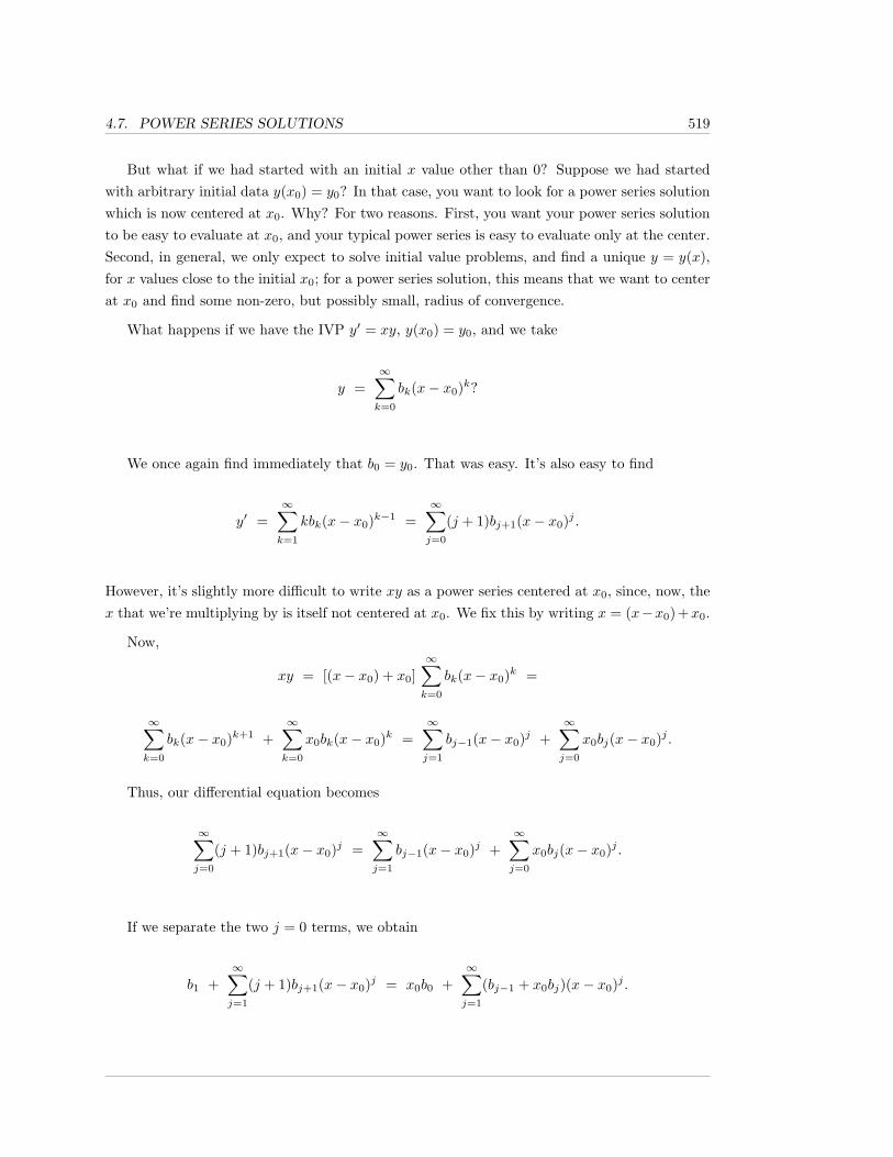
4.7. POWER SERIES SOLUTIONS 519
But what if we had started with an initial x value other than 0? Suppose we had startedwith arbitrary initial data y(x0) = y0? In that case, you want to look for a power series solutionwhich is now centered at x0. Why? For two reasons. First, you want your power series solutionto be easy to evaluate at x0, and your typical power series is easy to evaluate only at the center.Second, in general, we only expect to solve initial value problems, and find a unique y = y(x),for x values close to the initial x0; for a power series solution, this means that we want to centerat x0 and find some non-zero, but possibly small, radius of convergence.
What happens if we have the IVP y′ = xy, y(x0) = y0, and we take
y =∞∑k=0
bk(x− x0)k?
We once again find immediately that b0 = y0. That was easy. It’s also easy to find
y′ =∞∑k=1
kbk(x− x0)k−1 =∞∑j=0
(j + 1)bj+1(x− x0)j .
However, it’s slightly more difficult to write xy as a power series centered at x0, since, now, thex that we’re multiplying by is itself not centered at x0. We fix this by writing x = (x−x0) +x0.
Now,
xy = [(x− x0) + x0]∞∑k=0
bk(x− x0)k =
∞∑k=0
bk(x− x0)k+1 +∞∑k=0
x0bk(x− x0)k =∞∑j=1
bj−1(x− x0)j +∞∑j=0
x0bj(x− x0)j .
Thus, our differential equation becomes
∞∑j=0
(j + 1)bj+1(x− x0)j =∞∑j=1
bj−1(x− x0)j +∞∑j=0
x0bj(x− x0)j .
If we separate the two j = 0 terms, we obtain
b1 +∞∑j=1
(j + 1)bj+1(x− x0)j = x0b0 +∞∑j=1
(bj−1 + x0bj)(x− x0)j .
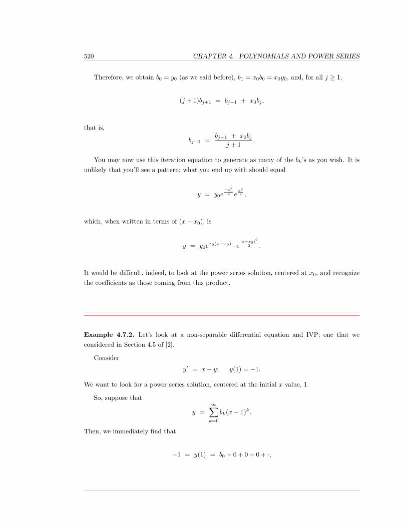
520 CHAPTER 4. POLYNOMIALS AND POWER SERIES
Therefore, we obtain b0 = y0 (as we said before), b1 = x0b0 = x0y0, and, for all j ≥ 1,
(j + 1)bj+1 = bj−1 + x0bj ,
that is,
bj+1 =bj−1 + x0bj
j + 1.
You may now use this iteration equation to generate as many of the bk’s as you wish. It isunlikely that you’ll see a pattern; what you end up with should equal
y = y0e−x20
2 ex22 ,
which, when written in terms of (x− x0), is
y = y0ex0(x−x0) · e
(x−x0)2
2 .
It would be difficult, indeed, to look at the power series solution, centered at x0, and recognizethe coefficients as those coming from this product.
Example 4.7.2. Let’s look at a non-separable differential equation and IVP; one that weconsidered in Section 4.5 of [2].
Consider
y′ = x− y; y(1) = −1.
We want to look for a power series solution, centered at the initial x value, 1.
So, suppose that
y =∞∑k=0
bk(x− 1)k.
Then, we immediately find that
−1 = y(1) = b0 + 0 + 0 + 0 + ·,
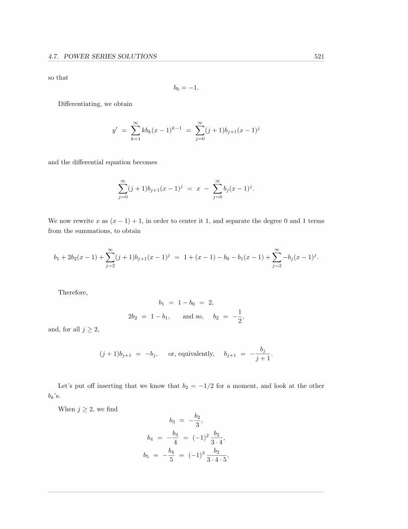
4.7. POWER SERIES SOLUTIONS 521
so thatb0 = −1.
Differentiating, we obtain
y′ =∞∑k=1
kbk(x− 1)k−1 =∞∑j=0
(j + 1)bj+1(x− 1)j
and the differential equation becomes
∞∑j=0
(j + 1)bj+1(x− 1)j = x −∞∑j=0
bj(x− 1)j .
We now rewrite x as (x− 1) + 1, in order to center it 1, and separate the degree 0 and 1 termsfrom the summations, to obtain
b1 + 2b2(x− 1) +∞∑j=2
(j + 1)bj+1(x− 1)j = 1 + (x− 1)− b0 − b1(x− 1) +∞∑j=2
−bj(x− 1)j .
Therefore,b1 = 1− b0 = 2,
2b2 = 1− b1, and so, b2 = −12,
and, for all j ≥ 2,
(j + 1)bj+1 = −bj , or, equivalently, bj+1 = − bjj + 1
.
Let’s put off inserting that we know that b2 = −1/2 for a moment, and look at the otherbk’s.
When j ≥ 2, we find
b3 = −b23,
b4 = −b34
= (−1)2 b23 · 4
,
b5 = −b45
= (−1)3 b23 · 4 · 5
,
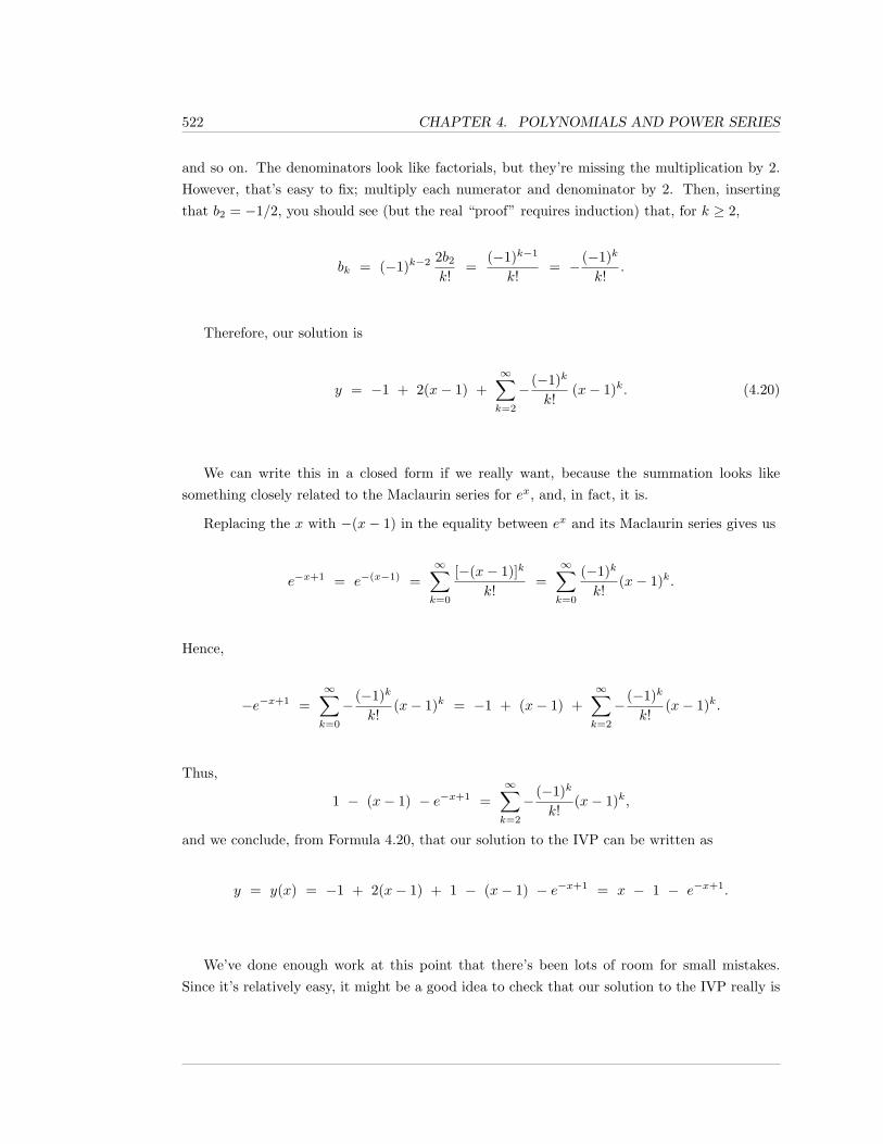
522 CHAPTER 4. POLYNOMIALS AND POWER SERIES
and so on. The denominators look like factorials, but they’re missing the multiplication by 2.However, that’s easy to fix; multiply each numerator and denominator by 2. Then, insertingthat b2 = −1/2, you should see (but the real “proof” requires induction) that, for k ≥ 2,
bk = (−1)k−2 2b2k!
=(−1)k−1
k!= − (−1)k
k!.
Therefore, our solution is
y = −1 + 2(x− 1) +∞∑k=2
− (−1)k
k!(x− 1)k. (4.20)
We can write this in a closed form if we really want, because the summation looks likesomething closely related to the Maclaurin series for ex, and, in fact, it is.
Replacing the x with −(x− 1) in the equality between ex and its Maclaurin series gives us
e−x+1 = e−(x−1) =∞∑k=0
[−(x− 1)]k
k!=
∞∑k=0
(−1)k
k!(x− 1)k.
Hence,
−e−x+1 =∞∑k=0
− (−1)k
k!(x− 1)k = −1 + (x− 1) +
∞∑k=2
− (−1)k
k!(x− 1)k.
Thus,
1 − (x− 1) − e−x+1 =∞∑k=2
− (−1)k
k!(x− 1)k,
and we conclude, from Formula 4.20, that our solution to the IVP can be written as
y = y(x) = −1 + 2(x− 1) + 1 − (x− 1) − e−x+1 = x − 1 − e−x+1.
We’ve done enough work at this point that there’s been lots of room for small mistakes.Since it’s relatively easy, it might be a good idea to check that our solution to the IVP really is
4.7. POWER SERIES SOLUTIONS 523
a solution.
We find
y(1) = 1− 1− e−1+1 = 0− 1 = −1,
which means that the initial data condition is satisfied. Also, if y = x − 1 − e−x+1, theny′ = 1 + e−x+1, and it is easy to verify that y′ = x− y.
Thus, we have indeed found a solution to the given initial value problem. In fact, we foundthe unique solution and, in this particular example, uniqueness is not difficult to establish.However, in more general IVP’s, showing that the solution is unique is not so easy, and we willnot go into the matter here.
What we have shown is that the unique real analytic solution at, or near, x = 1, is
y = x− 1− e−x+1.
Example 4.7.3. As our final example of this section, let’s look at a simple 2nd order differentialequation, with no initial conditions.
Consider
y′′ = −4y,
and we’ll look for a power series solution centered at 0.
So, suppose that y =∑∞k=0 bkx
k is a solution to our differential equation. We quickly find
y′ =∞∑k=1
kbkxk−1,
and
y′′ =∞∑k=2
k(k − 1)bkxk−2 =∞∑j=0
(j + 2)(j + 1)bj+2xj .
Therefore, we need∞∑j=0
(j + 2)(j + 1)bj+2xj =
∞∑j=0
−4bjxj .
524 CHAPTER 4. POLYNOMIALS AND POWER SERIES
It follows that y =∑∞k=0 bkx
k will be a solution to y′′ = −4y if and only if, for all j ≥ 0,
(j + 2)(j + 1)bj+2 = −4bj , or, equivalently, bj+2 = − 4bj(j + 2)(j + 1)
.
As the iteration formula above refers to an index which is 2 bigger on the left than the only bterm on the right, there will be one formula for the odd-indexed coefficients and another formulafor the even-indexed coefficients. In addition, b0 and b1 can each be anything at all.
Looking at the even coefficients first, we find
b2 = − 4b02 · 1
,
b4 = − 4b24 · 3
= (−1)2 42b04 · 3 · 2 · 1
,
b6 = − b46 · 5
= (−1)3 43b06 · 5 · 4 · 3 · 2 · 1
,
and, generally, for n ≥ 0,
b2n = (−1)n4nb0(2n)!
= b0 · (−1)n22n
(2n)!
A similar calculation shows that, for n ≥ 0,
b2n+1 = (−1)n4nb1
(2n+ 1)!= b1 · (−1)n
22n
(2n+ 1)!=
b12· (−1)n
22n+1
(2n+ 1)!
Therefore,
y =∞∑k=0
bkxk =
∑k even
bkxk +
∑k odd
bkxk =
∞∑n=0
b2nx2n +
∞∑n=0
b2n+1x2n+1 =
∞∑n=0
b0 · (−1)n22n
(2n)!x2n +
∞∑n=0
b12· (−1)n
22n+1
(2n+ 1)!x2n+1 =
4.7. POWER SERIES SOLUTIONS 525
b0 ·∞∑n=0
(−1)n(2x)2n
(2n)!+
b12·∞∑n=0
(−1)n(2x)2n+1
(2n+ 1)!.
If you look back at the equalities between cosx, sinx, and their Maclaurin series, you shouldsee that we just found that
y = b0 cos(2x) +b12
sin(2x),
which means that y(0) = b0 and y′(0) = b1, which would be determined by initial data.
We should remark that, above, when we split our summation into the even degree partsand the odd degree parts, we implicitly assumed that rearranging the order of the summationdid not affect the sum; in general, this requires that the series converges absolutely, as we shalldiscuss in Section 5.4.
Before we leave this section, we want to point out that the examples that we gave wereactually simple ones, though they may not have seemed so simple.
Consider, for instance, the problem of finding a power series solution to the differentialequation
y′ = y2 + x.
You can look for a power series solution, centered at 0, y =∑∞k=0 bkx
k, but what do you dowith the y2 part??? Well...you square your series, that is, you multiply it times itself, and usethe product series. Yes, it’s ugly, but it’s not ridiculously difficult to find at least the first fewterms of the solution.
What about solving
y′ = (sinx)y + x?
Again, what you have to do is fairly unpleasant; you let y =∑∞k=0 bkx
k and multiply this bythe Maclaurin series for sinx to deal with the (sinx)y part of the problem.
The point is: while solving differential equations via power series may be time-consuming andtedious, what you need to do, and actually doing it, is frequently/usually very straightforward.
526 CHAPTER 4. POLYNOMIALS AND POWER SERIES
4.7.1 Exercises
In each of Exercises 1 through 10, you are given an initial value problem, in which
the initial data is specified at a particular value x = x0. Assume that the initial
value problem has a unique power series solution, y =∑∞k=0 bk(x − x0)k (at least,
for x values near x0). (a) Determine iterative formulas for the bk. (b) Calculate b0
through b8 explicitly. (c) Approximate the value of your solution at x = x0 + 0.1 by
using the first 4 non-zero terms in your power series.
1. y′ = 5y + x; y(0) = 2
2. y′ = 5y + x; y(1) = 2
3. y′ = 5y + ex; y(0) = 2
4. y′ = 5y + xex; y(0) = 2
5. y′ = 5y + x2ex + 1; y(0) = 2
6. y′ = 5y + sinx; y(0) = 2
7. y′ = (x− 3)2y + 1; y(3) = −1
8. y′′ = 4y; y(0) = 1, y′(0) = 0
9. y′′ = 4y + 2ex; y(0) = 1, y′(0) = 0
10. y′′ = (x− 2)y + 1; y(2) = 1, y′(2) = 0
In each of Exercises 11 through 18, you are given an initial value problem, with
initial data specified at x = x0. Find a power series solution, centered at x0, and, by
manipulating known Maclaurin series, rewrite your solution in a “closed” form.
11. y′ = 5y + x; y(0) = 2
12. y′ = 5y + x; y(1) = 2
13. y′ = (x+ 2)2y; y(−2) = 7
14. y′ = 5y + ex−1; y(1) = 2
15. y′ = ay + bx; y(0) = 0, where a and b are constants, a 6= 0.
16. y′′ = 5y′; y(−2) = 7, y′(−2) = 0
17. y′′ = 4y; y(0) = 1, y′(0) = 0
4.7. POWER SERIES SOLUTIONS 527
18. y′′ = −k2y; y(0) = 1, y′(0) = 0, where k is a constant.
19. Find the 3rd order Maclaurin polynomial of the solution y = y(x) to the initial valueproblem
y′ = y2 + x; y(0) = 1.
20. Find the 3rd order Maclaurin polynomial of the solution y = y(x) to the initial valueproblem
y′ = y sinx + x; y(0) = 1.
528 CHAPTER 4. POLYNOMIALS AND POWER SERIES
Appendix 4.A Technical Matters
Theorem 4.A.1. Suppose that f and g are real analytic functions on an open interval I, andthat f(x) = g(x) for all x in an open interval J , which is contained in I. Then, f and g areequal on I.
Proof. By considering f − g, we are reduced to showing:
Suppose f is real analytic on an open interval I, and is 0 on an open subinterval J ⊆ I.Then, f is 0 on all of I.
We will use here that intervals are connected, i.e., that an interval is not the disjoint unionof two non-empty open sets.
We say that the germ of f is 0 at x if and only if there exists an open interval around x onwhich f is everywhere equal to 0; we write [f ]x = 0.
By definition, A = {x ∈ I | [f ]x = 0} is an open subset of I. By our assumption that f is 0on J , A is non-empty. We claim that the set B = {x ∈ I | [f ]x 6= 0}, which is the complementof A in I, is also open. As I is connected, it will follow that B is empty, i.e., that f is zero onall of I.
Suppose that b ∈ B. We wish to show that there is an open interval K around b such thatK ⊆ B. Suppose not. Then, by picking smaller and smaller open intervals around b, we canproduce a sequence of points ai ∈ A such that limi→∞ ai = b. As f is real analytic at eachai and is zero on an open interval around ai, all of the coefficients of the Taylor series of fat each ai must be 0, i.e., for all i, for all k, f (k)(ai) = 0. As the derivatives are continuous,f (k)(b) = limi→∞ f (k)(ai) = 0. As all of the derivatives f (k)(b) are 0, and f is real analytic atb, it follows that f is 0 in an open interval around b, i.e., b 6∈ B. This contradiction shows thatB would have to be open and, hence, empty.
Chapter 5
Theorems on Sequences andSeries
As we have discussed in prior chapters, with various levels of formalism, a sequence of realnumbers is essentially just an infinite list of real numbers, that is, for all integers n, greaterthan or equal to some initial integer m, we have a real number bn. A sequence converges if andonly if limn→∞ bn exists, where n is allowed to take on only integer values ≥ m. Convergenceof certain kinds of sequences is a fundamental property of the real numbers, which we shall notattempt to derive.
An infinite series is what you get when you add an infinite sequence of terms; it’s a limit ofpartial sums. We will discuss many tests for deciding when such limits of partial sums exist.
Unfortunately, while it is extremely important to distinguish between sequences and series,confusion between these two terms is common – perhaps stemming from the fact that bothwords start with “se” or, perhaps, because the partial sums themselves form a second sequence,in addition to the sequence of terms. Throughout this chapter, you need to keep in mind that,in an infinite series, you are trying to make sense of an infinite sum; this is the limit of thepartial sums, not the limit of the individual summands (the terms).
529
530 CHAPTER 5. THEOREMS ON SEQUENCES AND SERIES
5.1 Theorems on Sequences
In our discussion and use of power series, and several other times throughout this textbook, wehave used infinite sequences, “lists” of real numbers that never stop. In this section, we willstate, prove, and look at examples of some fundamental definitions and results on sequences.
Informally, a sequence of real numbers is a list of real numbers, the terms, such that there’s afirst number, a second number, a third number, and so on – in general, there’s an n-th numberin the list, for every natural number n.
For instance, we sometimes list a few numbers in the list, with some obvious pattern, andthen, once the pattern is clear, we indicate the remainder of the list with dots, e.g.,
1,12,
13,
14, . . . ,
where the n-th term is bn = 1/n.
It is convenient in some cases to start the subscript, the index, at some number other than1; for instance, we might consider the sequence given by
an =1
(n− 1)(n− 2), for n ≥ 3.
This causes some mild confusion when speaking of the terms of the sequence, because it’s thentrue that the first term of this sequence is a3, the second term is a4, and so on. The problem is:if you said “the n-th term”, when using n for the indexing variable, it might be unclear whetheryou meant an or an+2. For this reason, it’s best to talk about an, which is very clear, ratherthan to use common English phrasing. Typically, we care about the limit of a sequence, as theindex approaches ∞, so confusing an and an+2 is unlikely to cause a problem.
The notion of a sequence as a list is informal. Really, a sequence is a function; you pickan integer (greater than or equal to some starting integer m), and you get back a real number.We gave the rigorous definitions of a sequence and its convergence/divergence in [2], and inDefinition 4.5.1; however, we will give those definitions again here.
5.1. THEOREMS ON SEQUENCES 531
Definition 5.1.1. Suppose that m is an integer, i.e., is in the set Z. Denote by Z≥m theset of integers which are greater than or equal to m.
A function b : Z≥m → R is called a sequence (of real numbers). In place of b(n), itis standard to write bn.
We say that the sequence bn converges to (a real number) L, and writelimn→∞ bn = L if and only if, for all ε > 0, there exists an integer N ≥ m such that,for all integers n ≥ N , |bn − L| < ε.
If a sequence does not converge to some real number L, then we say that the sequencediverges.
The sequence bn diverges to ∞, and we write limn→∞ bn = ∞, if and only if, for allreal numbers A, there exists N ≥ m such that, for all n ≥ N , bn > A.
The sequence bn diverges to −∞, and we write limn→∞ bn = −∞, if and only if, forall real numbers A, there exists N ≥ m such that, for all n ≥ N , bn < A.
It is important that a sequence can have only one limit.
Theorem 5.1.2. If a sequence bn converges to L1 and converges to L2, then L1 = L2, i.e.,if a sequence converges to some limit, then that limit is the unique limit.
Proof. This proof is identical to the proof of uniqueness of limits of functions of a real variable,except that you allow only integers for the value of the variable. We refer you to the proof in[2].
Remark 5.1.3. Because the same notation is used for limits over the integers and limits overthe real numbers, some confusion can arise.
Think about limn→∞ sin(nπ). Do we mean the limit of the sequence an = sin(nπ), so thatn takes on only integer values (with an unspecified starting value)? Or do we mean that n canbe any real number? It makes a difference.
If we mean that n varies over the real numbers, then limn→∞ sin(nπ) does not exist, becausethe sine function continues to oscillate between −1 and 1 as n increases through the real numbers.
On the other hand, if n is an integer, then sin(nπ) = 0, and so the limit limn→∞ sin(nπ) of
the sequence sin(nπ) is just limn→∞ 0 = 0.
532 CHAPTER 5. THEOREMS ON SEQUENCES AND SERIES
How do we avoid this confusion? There are several ways. One is to explicitly state that weare taking the limit of a sequence. Another is to refer to n’s that take on only integer values asdiscrete variables, and n’s that can take on arbitrary real values as continuous variables. Finally,it is common to use the letters i, j, k, l, m, and n as discrete variables, and the letters r, s t, u,v, w, x, y, and z as continuous variables. One of these ways should always make it clear whichtype of limit is intended.
For instance, many people would write simply
limn→∞
sin(nπ) = limn→∞
0 = 0,
whilelimx→∞
sin(xπ) does not exist,
automatically assuming that n denotes a discrete variable and x denotes a continuous variable.
In the above remark, we saw that, if we take the function f(x) = sin(xπ), whose domainis the set of real numbers, then limx→∞ f(x) does not exist, but if we restrict the domain off to the integers, then limn→∞ f(n) does exist. However, the theorem below tells us that, iflimx→∞ f(x) exists, and equals L, then limn→∞ f(n) also exists and equals L.
Theorem 5.1.4. Suppose that M is real number and that f(x) is defined for all real x ≥M .If limx→∞ f(x) exists as an extended real number, and equals L, then the limit
limn→∞ f(n) of the restriction of f to the integers ≥ M exists as an extended real numberand equals L.
Proof. We shall prove the case in which L is a real number, and leave the cases where L = ±∞as an exercise.
Suppose that limx→∞ f(x) equals a real number L, and let ε > 0. Then, there exists a realnumber N ≥M such that, if x is a real number and x > N , then |f(x)− L| < ε. However, thisis true for all real numbers > N ; in particular, it’s true for the integers > N .
This is precisely what it means for the sequence f(n) to converge to L.
5.1. THEOREMS ON SEQUENCES 533
Example 5.1.5. Theorem 5.1.4 is very useful when trying to calculate limits of sequences whicharise from restricting functions of a continuous variable.
An easy example is to consider g(x) = 1/x. Then, we know that limx→∞ g(x) = 0. It followsthat
limn→∞
1n
= 0,
where, in this latter limit, we mean the limit of the sequence.
Example 5.1.6. Let’s look at something a bit more complicated. Consider the limit of thesequence n/en.
We’d like to use l’Hopital’s Rule (see [2]), but l’Hopital’s Rule requires us to take derivativesof the numerator and denominator. If n really takes on only integer vales, then we can’t takederivatives.
However, consider, instead, the function of a continuous variable f(x) = x/ex. Then,l’Hopital’s Rule tells us
limx→∞
x
ex= lim
x→∞
x′
(ex)′= lim
x→∞
1ex
= 0,
and now Theorem 5.1.4 tells us that, because the “continuous limit” above is 0, we also havethe discrete limit equaling the same thing, i.e.,
limn→∞
n
en= 0.
Understanding that the existence of the continuous variable limit implies the existence (andequality) of the discrete variable limit, it is fairly standard to be a bit sloppy, and never writeanything explicit about the continuous variable function, but rather simply apply l’Hopital’sRule to the function containing the discrete variable n. That is, it’s pretty standard to write
limn→∞
n
en= lim
n→∞
n′
(en)′= lim
n→∞
1en
= 0.
Just remember: there’s really a theorem at work here.
534 CHAPTER 5. THEOREMS ON SEQUENCES AND SERIES
Many of the results that we proved for limits limx→∞ f(x) have analogs for sequences, whichcan be proved simply by replacing the continuous variable x by the discrete variable n; suchresults include arithmetic with limits, the Pinching Theorem, and composition with continuousfunctions, all of which we state below.
Theorem 5.1.7. (Arithmetic of Convergent Sequences) Suppose that the sequencesan and bn converge, and that c is a constant. Then,
1. limn→∞ c = c;
2. limn→∞(an + bn) = limn→∞ an + limn→∞ bn;
3. limn→∞ can = c · limn→∞ an;
4. limn→∞(an · bn) = limn→∞ an · limn→∞ bn;
5. limn→∞
anbn
=limn→∞ anlimn→∞ bn
, provided that limn→∞ bn 6= 0.
In particular, the sequences an + bn, can, an · bn, and an/bn converge.
Example 5.1.8. Since we know that
limn→∞
1n
= 0,
multiplying this limit times itself two and three times gives us that
limn→∞
1n2
= 0 and limn→∞
1n3
= 0.
Combining these with Properties 1-4 in Theorem 5.1.7 tells us that
limn→∞
[(5 − 7
n2
)(3 +
4n3
)]= (5− 7 · 0)(3 + 4 · 0) = 15.
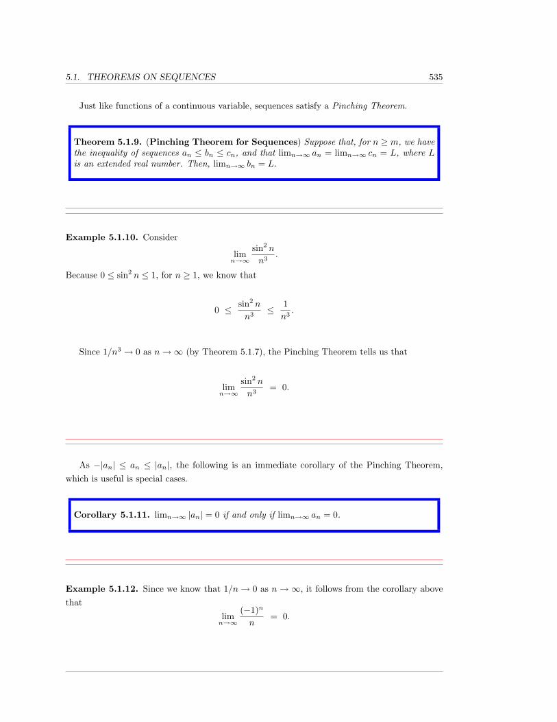
5.1. THEOREMS ON SEQUENCES 535
Just like functions of a continuous variable, sequences satisfy a Pinching Theorem.
Theorem 5.1.9. (Pinching Theorem for Sequences) Suppose that, for n ≥ m, we havethe inequality of sequences an ≤ bn ≤ cn, and that limn→∞ an = limn→∞ cn = L, where Lis an extended real number. Then, limn→∞ bn = L.
Example 5.1.10. Consider
limn→∞
sin2 n
n3.
Because 0 ≤ sin2 n ≤ 1, for n ≥ 1, we know that
0 ≤ sin2 n
n3≤ 1
n3.
Since 1/n3 → 0 as n→∞ (by Theorem 5.1.7), the Pinching Theorem tells us that
limn→∞
sin2 n
n3= 0.
As −|an| ≤ an ≤ |an|, the following is an immediate corollary of the Pinching Theorem,which is useful is special cases.
Corollary 5.1.11. limn→∞ |an| = 0 if and only if limn→∞ an = 0.
Example 5.1.12. Since we know that 1/n→ 0 as n→∞, it follows from the corollary abovethat
limn→∞
(−1)n
n= 0.
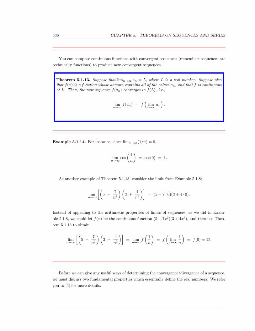
536 CHAPTER 5. THEOREMS ON SEQUENCES AND SERIES
You can compose continuous functions with convergent sequences (remember: sequences aretechnically functions) to produce new convergent sequences.
Theorem 5.1.13. Suppose that limn→∞ an = L, where L is a real number. Suppose alsothat f(x) is a function whose domain contains all of the values an, and that f is continuousat L. Then, the new sequence f(an) converges to f(L), i.e.,
limn→∞
f(an) = f(
limn→∞
an
).
Example 5.1.14. For instance, since limn→∞(1/n) = 0,
limn→∞
cos(
1n
)= cos(0) = 1.
As another example of Theorem 5.1.13, consider the limit from Example 5.1.8:
limn→∞
[(5 − 7
n2
)(3 +
4n3
)]= (5− 7 · 0)(3 + 4 · 0).
Instead of appealing to the arithmetic properties of limits of sequences, as we did in Exam-ple 5.1.8, we could let f(x) be the continuous function (5− 7x2)(3 + 4x3), and then use Theo-rem 5.1.13 to obtain
limn→∞
[(5 − 7
n2
)(3 +
4n3
)]= lim
n→∞f
(1n
)= f
(limn→∞
1n
)= f(0) = 15.
Before we can give any useful ways of determining the convergence/divergence of a sequence,we must discuss two fundamental properties which essentially define the real numbers. We referyou to [3] for more details.
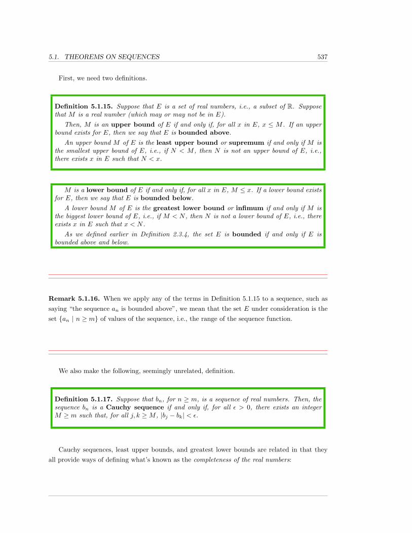
5.1. THEOREMS ON SEQUENCES 537
First, we need two definitions.
Definition 5.1.15. Suppose that E is a set of real numbers, i.e., a subset of R. Supposethat M is a real number (which may or may not be in E).
Then, M is an upper bound of E if and only if, for all x in E, x ≤ M . If an upperbound exists for E, then we say that E is bounded above.
An upper bound M of E is the least upper bound or supremum if and only if M isthe smallest upper bound of E, i.e., if N < M , then N is not an upper bound of E, i.e.,there exists x in E such that N < x.
M is a lower bound of E if and only if, for all x in E, M ≤ x. If a lower bound existsfor E, then we say that E is bounded below.
A lower bound M of E is the greatest lower bound or infimum if and only if M isthe biggest lower bound of E, i.e., if M < N , then N is not a lower bound of E, i.e., thereexists x in E such that x < N .
As we defined earlier in Definition 2.3.4, the set E is bounded if and only if E isbounded above and below.
Remark 5.1.16. When we apply any of the terms in Definition 5.1.15 to a sequence, such assaying “the sequence an is bounded above”, we mean that the set E under consideration is theset {an | n ≥ m} of values of the sequence, i.e., the range of the sequence function.
We also make the following, seemingly unrelated, definition.
Definition 5.1.17. Suppose that bn, for n ≥ m, is a sequence of real numbers. Then, thesequence bn is a Cauchy sequence if and only if, for all ε > 0, there exists an integerM ≥ m such that, for all j, k ≥M , |bj − bk| < ε.
Cauchy sequences, least upper bounds, and greatest lower bounds are related in that theyall provide ways of defining what’s known as the completeness of the real numbers:
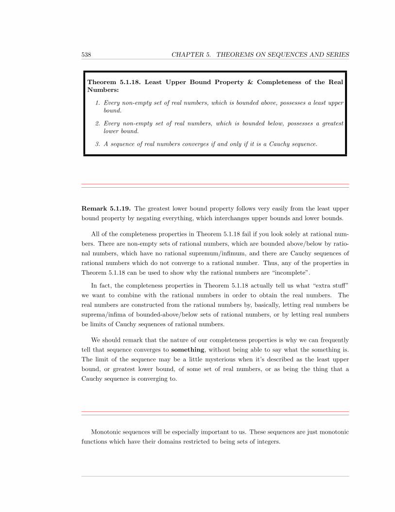
538 CHAPTER 5. THEOREMS ON SEQUENCES AND SERIES
Theorem 5.1.18. Least Upper Bound Property & Completeness of the RealNumbers:
1. Every non-empty set of real numbers, which is bounded above, possesses a least upperbound.
2. Every non-empty set of real numbers, which is bounded below, possesses a greatestlower bound.
3. A sequence of real numbers converges if and only if it is a Cauchy sequence.
Remark 5.1.19. The greatest lower bound property follows very easily from the least upperbound property by negating everything, which interchanges upper bounds and lower bounds.
All of the completeness properties in Theorem 5.1.18 fail if you look solely at rational num-bers. There are non-empty sets of rational numbers, which are bounded above/below by ratio-nal numbers, which have no rational supremum/infimum, and there are Cauchy sequences ofrational numbers which do not converge to a rational number. Thus, any of the properties inTheorem 5.1.18 can be used to show why the rational numbers are “incomplete”.
In fact, the completeness properties in Theorem 5.1.18 actually tell us what “extra stuff”we want to combine with the rational numbers in order to obtain the real numbers. Thereal numbers are constructed from the rational numbers by, basically, letting real numbers besuprema/infima of bounded-above/below sets of rational numbers, or by letting real numbersbe limits of Cauchy sequences of rational numbers.
We should remark that the nature of our completeness properties is why we can frequentlytell that sequence converges to something, without being able to say what the something is.The limit of the sequence may be a little mysterious when it’s described as the least upperbound, or greatest lower bound, of some set of real numbers, or as being the thing that aCauchy sequence is converging to.
Monotonic sequences will be especially important to us. These sequences are just monotonicfunctions which have their domains restricted to being sets of integers.
5.1. THEOREMS ON SEQUENCES 539
Definition 5.1.20. Suppose that bn, for n ≥ m, is a sequence of real numbers.
• bn is increasing if and only if, for all integers k and l such that k ≥ l ≥ m, bk ≥ bl.
• bn is decreasing if and only if, for all integers k and l such that k ≥ l ≥ m, bk ≤ bl.
• bn is monotonic if and only if it is increasing or decreasing.
Remark 5.1.21. Note that increasing sequences are automatically bounded below by the initialterm of the sequence, and decreasing sequences are automatically bounded above by the initialterm of the sequence.
Therefore, the assumption that an increasing sequence is bounded is equivalent to the as-sumption that it’s bounded above, and the assumption that a decreasing sequence is boundedis equivalent to the assumption that it’s bounded below.
When you’re interested in whether or not a sequence converges, you can ignore any finitenumber of initial terms in the sequence. Hence, the following terminology is frequently conve-nient to use.
Definition 5.1.22. We say that a sequence an, for n ≥ m, eventually has a certainproperty if there exists an integer M ≥ m such that the new sequence an, for n ≥ M , hasthe property.
Thus, for instance, a sequence is eventually increasing if it is always increasing after somepoint.
The following theorem gives one of the most basic ways in which one concludes that a seriesconverges.
540 CHAPTER 5. THEOREMS ON SEQUENCES AND SERIES
Theorem 5.1.23. Suppose that a sequence bn, for n ≥ m, is eventually monotone. Then,bn converges if and only if it is bounded.
More specifically,
1. if bn is increasing for n ≥ m,
a. if limn→∞ bn = L, then, for all n ≥ m, bm ≤ bn ≤ L, and
b. if, for all n ≥ m, bn ≤ B, then limn→∞ bn exists and is ≤ B.
2. if bn is decreasing for n ≥ m,
a. if limn→∞ bn = L, then, for all n ≥ m, L ≤ bn ≤ bm, and
b. if, for all n ≥ m, B ≤ bn, then limn→∞ bn exists and is ≥ B.
In particular, the only way for an eventually increasing sequence to diverge is to diverge to∞, and the only way for an eventually decreasing sequence to diverge is to diverge to −∞.This means that, for every eventually monotone sequence bn, we can write limn→∞ bn = L,where L is an extended real number, i.e., a real number or ±∞.
Proof. Assume that the sequence is increasing for all n ≥M . The decreasing case is completelyanalogous.
Suppose that bn converges to L. We will show that, for all n ≥ M , bn ≤ L. Since thesequence is increasing for n ≥ M , this will show that the sequence bn is bounded below by theminimum value in the set {bn | m ≤ n ≤M} and above by the maximum of L and the maximumvalue in the set {bn | m ≤ n ≤M − 1}.
Suppose, to the contrary, that there exists n0 ≥M such that bn0 > L. Let ε = bn0 − L > 0.As bn is increasing for n ≥M , for all n ≥ n0,
bn − L ≥ bn0 − L ≥ ε.
This contradicts that L is the limit of the sequence, and this contradiction establishes thatsequence bn is bounded.
We need now to show the other direction in the proof. So, suppose that the sequence bn,n ≥ m is bounded. Then, the set E = {bn | n ≥M} is bounded; let B be an upper bound of E.By Theorem 5.1.18, E has a least upper bound; call it L, which is necessarily ≤ B. We claimthat limn→∞ bn = L.
Note, first, that, since L is an upper bound for E, for all n ≥ M , bn ≤ L, i.e., L − bn ≥ 0.Now, let ε > 0. Then, L− ε, which is less than L is not an upper bound of E, i.e., there exists
5.1. THEOREMS ON SEQUENCES 541
n0 ≥M such that bn0 > L− ε. This means that L− bn0 < ε. As bn is increasing for n ≥M , itfollows that, for all n ≥ n0, L− bn < ε. As L− bn ≥ 0, this establishes what we wanted: for alln ≥ n0, |L− bn| < ε.
We still need to make an argument to justify the last statement in the theorem. Supposenow only that bn is increasing for all n ≥M . Then, as we saw above, bn is bounded below by theminimum value in the set {bn | m ≤ n ≤M}. As we also saw above, if the sequence bn diverges,then it’s unbounded; thus, it must not be bounded above. Pick some real number A, and let A0
be the maximum of A and 1 plus the maximum value in the set {bn | m ≤ n ≤ M − 1}. As bnis not bounded above, there exists n0 ≥M such that bn0 ≥ A0. As bn, for n ≥M , is increasing,it follows that, for all n ≥ n0, bn ≥ bn0 ≥ A0 ≥ A, which shows that bn diverges to ∞.
Corollary 5.1.24. (Comparison of Monotonic Sequences)
1. Suppose that, for n ≥ m, an and bn are increasing, and an ≤ bn. Then, if bn converges,so does an and, in this case, limn→∞ an ≤ limn→∞ bn; in particular, if an diverges,then so does bn.
2. Suppose that, for n ≥ m, an and bn are decreasing, and an ≤ bn. Then, if anconverges, so does bn and, in this case, limn→∞ an ≤ limn→∞ bn; in particular, if bndiverges, then so does an.
Proof. This is immediate from Theorem 5.1.23.
Example 5.1.25. Let’s look at an example which is relevant to the next section, where we lookat infinite series.
For n ≥ 0, define sequences
an =n∑k=0
12k + 1
and bn =n∑k=0
12k.
As we are adding something non-negative to get from one term of an to the next, and somethingnon-negative to get from one term of bn to the next, the sequences an and bn are both increasing.Moreover, clearly, we have an ≤ bn (in fact, an < bn). We also know from Theorem 4.4.10 thatthe sequence bn converges to 2.
It follows from Corollary 5.1.24 that the sequence an converges to something ≤ 2, but wehave no idea what that something is – though the something must also be greater than or equal
542 CHAPTER 5. THEOREMS ON SEQUENCES AND SERIES
to every an. In fact, the limit of the sequence an is precisely the smallest number that is greaterthan or equal to all of the an’s, i.e., the least upper bound of the sequence.
Consider now the sequence 1/n, for n ≥ 1; this the harmonic sequence:
11,
12,
13,
14,
15,
16,
17,
18
. . . .
Suppose that we look at just the terms in the harmonic sequence that have even denominators:
12,
14,
16,
18,
110,
112,
114,
116
. . . .
This is the sequence 1/(2n), for n ≥ 1. Notice that each of the terms in this even harmonicsequence appear in the harmonic sequence, and they appear in the same order, i.e., the evenharmonic sequence is obtained from deleting terms from the harmonic series, without rearrangingthe remaining terms.
Sequences obtained in this manner are call subsequences.
Definition 5.1.26. Suppose that we have a sequence an, for n ≥ m. A subsequence ofthe sequence an is a sequence formed by taking some (or all) of the terms of an in order.Rigorously, this means that a subsequence of an, for n ≥ m, is a sequence ank , where nk,for k ≥ 1, is a sequence of integers such that n1 ≥ m and, for i < j, ni < nj, i.e., theindices in the subsequence are a strictly increasing sequence of some of the indices from thesequence an.
There is a theorem and a corollary about subsequences that will be of interest to us.
Theorem 5.1.27. If limn→∞ an = L, where L is an extended real number, then the limitof every subsequence of an is also L.
In particular, if a sequence an has two (or more) subsequences which have different limits,then an diverges.
Proof. While we could write this in full mathematical detail, that would obscure what’s reallygoing on, which is very elementary.
5.1. THEOREMS ON SEQUENCES 543
Suppose that limn→∞ an = L. This means that you can make an as close to L as you want(or, in the cases where L = ±∞, you can make L as big or as negative as you want) by pickingthe index n to be big enough. But, this is true for every an as long as the index is big enough;in particular, it would be true for the indices (which are big enough) of the a’s appearing in anysubsequence.
Recall from Theorem 5.1.23 that a monotone sequence always approaches a limit L, if weallow extended real numbers L. Combining this with the theorem above, we immediately obtain:
Corollary 5.1.28. If a sequence an is monotonic, and a subsequence of an has an extendedreal number L as its limit, then limn→∞ an = L.
Example 5.1.29. Consider the sequence an, for n ≥ 1, an =1n
+ (−1)n.
If we look at the subsequence where n is even, i.e., where n = 2k, k ≥ 1, we find that
a2k =12k
+ (−1)2k =12k
+ 1,
which clearly approaches 1 as k →∞.
On the other hand, if we look at the subsequence where n is odd, i.e., where n = 2k − 1,k ≥ 1, we find that
a2k−1 =1
2k − 1+ (−1)2k−1 =
12k − 1
− 1,
which clearly approaches −1 as k →∞.
As there are two sequences of an which approach different limits, the (entire) sequence andiverges, by Theorem 5.1.27.
544 CHAPTER 5. THEOREMS ON SEQUENCES AND SERIES
5.1.1 Exercises
In each of Exercises 1 through 15, determine whether the given sequence converges
or diverges. If the sequence converges, find its limit. As we are interested in what
happens as n→∞, we do not specify an initial n value; assume that n is big enough
so that all of the given terms are defined.
1. 1 +5n
2.5 + 3nn
3.n2
n2 + 1
4.2n + n2
2n
5.2n cos
(nπ4
)n2 + 1
6.n
10 lnn
7. ln(2n)− ln(n+ 1)
8.2n√n2 + 3
9.(
7 +1n
)1/n
10.(
1 +3n
)n11.
(5 + n)n
nn
12.en
n!
13.100n
n!
14. tan−1 n
15. n−√n2 + 7
In each of Exercises 16 through 19, use the Pinching Theorem, Theorem 5.1.9, to show that thegiven sequence converges.
5.1. THEOREMS ON SEQUENCES 545
16.2 + (−1)n
n
17.5 sinn+ 7
n2
18.3 sinn− 2 cosn√
n+ 1
19.4n+ 3(−1)n
n
In each of Exercises 20-24, find two subsequences of the given sequence which converge todifferent limits. Conclude that each sequence diverges.
20. 2 + (−1)n
21. sin(nπ4
)22.
2n cos(nπ4
)n+ 1
23. 12 , − 1
2 , 23 , − 2
3 , 34 , − 3
4 , 45 , − 4
5 , . . .
24. 21 , 0, 0, 3
2 , 0, 0, 0, 43 , 0, 0, 0, 0, 5
4 , 0, 0, 0, 0, 0, 65 , . . .
25. Suppose that a sequence an, n ≥ m, has the property that, for all n ≥ m, an ≤ 7.
a. Is it true that the sequence must converge to a number that’s ≤ 7? Prove it or givea counterexample.
b. Is it true that, if the sequence converges to L, then L ≤ 7? Prove it or give acounterexample.
c. Is it true that, if an is increasing, then it converges to a number that’s ≤ 7? Prove itor give a counterexample.
26. Suppose that a sequence an, n ≥ m, has the property that, for all n ≥ m, 3 ≤ an ≤ 7.
a. Is it true that the sequence must converge to a number L such that 3 ≤ L ≤ 7? Proveit or give a counterexample.
b. Is it true that, if the sequence converges to L, then 3 ≤ L ≤ 7? Prove it or give acounterexample.
c. Is it true that, if an is monotonic, then it converges to a number L such that 3 ≤L ≤ 7? Prove it or give a counterexample.
546 CHAPTER 5. THEOREMS ON SEQUENCES AND SERIES
27. Suppose that the sequence an converges, and that the sequence bn diverges. Prove thatthe sequence an + bn diverges.
28. Give an example of a sequence an which diverges, and a sequence bn which diverges suchthat the sequence an + bn converges.
29. Suppose that the sequence an converges to a non-zero limit, and that the sequence bn
diverges. Prove that the sequence bn/an diverges.
30. Perhaps the most famous sequence of all time is the Fibonacci sequence, Fn, n ≥ 0, givenby:
0, 1, 1, 2, 3, 5, 8, 13, 21, . . . ,
where the sequence is given iteratively by specifying that F0 = 0, F1 = 1, and, for alln ≥ 2,
Fn = Fn−1 + Fn−2.
That is, after the first two terms, each term is the sum of the two terms before it. In thisexercise, we will look at a closed (non-iterative) formula for Fn.
a. Suppose that a and b are constants. Consider the sequence cn, n ≥ 0, given by
cn = a
(1 +√
52
)n+ b
(1−√
52
)n.
Determine a and b so that c0 = 0 and c1 = 1.
b. Show that
(1 +√
52
)2
=3 +√
52
and
(1−√
52
)2
=3−√
52
.
c. Using the constants a and b that you found in part (a), show that that the sequencecn in part (a) is, in fact, the Fibonacci sequence Fn. Since you know that c0 = 0,and c1 = 1, to show that cn = Fn, you need to show that cn satisfies the Fibonacciiteration formula, i.e., you need to show that,for n ≥ 2,
cn = cn−1 + cn−2.
5.1. THEOREMS ON SEQUENCES 547
d. Calculatelimn→∞
Fn+1
Fn.
The value that you obtain for this limit is known as the Golden Ratio.
While they may appear to be simply interesting mathematical curiosities, the Fibonaccisequence and the Golden Ratio surprisingly appear frequently in nature, for example, inthe arrangements of leaves on a plant and in the spiral shell of a nautilus.
548 CHAPTER 5. THEOREMS ON SEQUENCES AND SERIES
5.2 Theorems on Series I:Basic Properties
In the last few sections of the previous chapter, we looked at infinite sums in the guise of powerseries. For a power series function p(x) =
∑∞k=0 ck(x− a)k, we are interested in convergence of
the series for different x values. But, for any fixed value of x, a power series simply becomes asummation
∑bk of a sequence of numbers bk, and we can forget that the sequence of number
that we’re adding are of the form bk = ck(x−a)k; that is, we can forget that the sequence comesfrom the terms of a power series. Such a summation of fixed numbers is simply called a series oran infinite series; to emphasize that the terms are not changing as a function of some variablex, the terminology series of constants is often used.
When we discussed series earlier, we put off any discussion of general convergence theorems,other than the Ratio Test, Theorem 4.5.13, though we did also look at the convergence of a fewspecific series; in these latter cases, we established convergence by showing that certain functionsequal their Taylors series in Section 4.4.
In this section, we will state, but (usually) not prove a large number of results on convergenceand divergence of series of constants. Starting with an infinite sequence bk, for k ≥ m, we addmore and more terms of the sequence together in the partial sums, and see if these partial sumsapproach anything; if they do, then that thing is, by definition, the sum of the series
∑∞k=m bk,
and we say that the series converges to, or equals, this limit. This means that a series is, infact, the limit of a sequence, but it’s the limit of the sequence of partial sums, not the sequenceof terms.
The theorems that we shall state are usually referred to as tests for convergence or divergence.
Even though we gave following definition before in Definition 4.5.3, it is appropriate to giveit again here. After the definition, we also repeat some of the comments that we made earlier,because these comments are vitally important to understanding infinite series.
Definition 5.2.1. Given a sequence bk, for k ≥ m, we define, for each n ≥ m, the partialsum to be
∑nk=m bk, and the infinite sum or infinite series or, simply, series to be
the infinite summation∑∞k=m bk, which, technically, consists of the sequence bk together
with the summation instruction/symbol, telling you to add the sequence. The terms of thesequence being added are also referred to as the terms of the series.
5.2. BASIC THEOREMS ON SERIES 549
The sum of the series or value of the series∑∞k=m bk is the limit as n → ∞ of the
partial sums, and we write∞∑k=m
bk = limn→∞
n∑k=m
bk,
provided the limit exists, in which case we say that the partial sums converge, that theseries converges, or simply that the infinite sum exists and is equal to the limit of thepartial sums.
If the limit of the partial sums does not exist, then we say that the series diverges or,simply, that the infinite sum does not exist.
Note that there are actually two sequences associated with an infinite sum/series: the se-quence of things you’re adding, the terms, and the sequence of partial sums sn =
∑nk=m bk.
What we’re interested in is what happens to the sequence of partial sums as n→∞.
As with approximating Taylor series by Taylor polynomials, the partial sums of any infiniteseries are frequently used as approximations of the infinite summation, assuming that the infinitesum exists, i.e., assuming that the series converges.
We are trying to define what an infinite sum should mean. Intuitively, it means the limitas you add more and more terms; this means that an infinite sum is the limit of the partialsums, NOT the limit of the terms. The terms are just the individual summands; they arenot sums themselves.
Remark 5.2.2. You may wonder about the difference between a series and its value or sum.Technically, a series is actually the sequence, together with the summation sign(s), indicatingthat you want to add the given sequence, and the value or sum is what you get when you actuallydo the summation, i.e., the limit of the partial sums.
What’s the point? Well...even though∑∞k=1
12k
= 1 (look back at Theorem 4.4.10 and usea = 1/2 and x = 1/2), you shouldn’t talk about the series that consists of just the number 1.The series means the sum written out as a sum of the terms; its value is just a number (providedthe series converges).
Fortunately, this distinction seems to cause no problem; when people discuss infinite series,there is always a clear sequence being summed.
One last point, which may be obvious. When we write something like∑∞k=1
12k
= 1, thereis no need to assert separately that the series
∑∞k=1
12k
converges; we’ve already stated what itconverges to.
550 CHAPTER 5. THEOREMS ON SEQUENCES AND SERIES
Okay. So, given an infinite series of constants, how do you find the sum? You might say“that’s easy – just take the limit of the partial sums”. The problem, and it’s a big one, is thatthere are very few series, or types of series, for which we can write nice, manageable expressionsfor the partial sums. In fact, basically, there are only two kinds of series for which formulas forthe partial sums are easy to obtain: geometric series and telescoping series.
Using different terminology, we derived the formula for the partial sums of geometric seriesway back in Corollary 2.1.11, and we looked at geometric series themselves in Theorem 4.4.10.However, we wish to restate these results now, using a different letter r for the base.
Theorem 5.2.3. Consider the geometric series∑∞k=0 ar
k and the sequence of partial sumssn =
∑nk=0 ar
k, for n ≥ 0.
1. If r 6= 1, then,
sn = a · 1− rn+1
1− r.
2. If |r| < 1, then the series converges to a/(1− r), that is
∞∑k=0
ark =a
1− r.
3. If |r| ≥ 1 and a 6= 0, then the series diverges.
Example 5.2.4. A classic social problem arises when a number of people are at dinner, andthere’s one piece of bread left. No one wants to take the entire remaining piece, and so eachperson rips off part of the bread and takes that piece, leaving some behind.
Let’s suppose that we start with one piece of bread, and that each person who takes somebread takes 1/3 of the remaining bread. What do we get if we keep track of the total bread taken(as fractions of the initial 1 piece) and the total bread remaining, assuming that this thirding-process goes on forever (ignoring that this is physically impossible and/or that we would at somepoint split atoms and blow up everything).
The first person takes 1/3, leaving behind 2/3. The second person takes 1/3 of the remaining2/3, so (1/3)(2/3) of the original one piece, leaving behind (2/3)(2/3) = (2/3)2. The third persontakes (1/3)(2/3)2, leaving behind (2/3)(2/3)2 = (2/3)3, and so on.
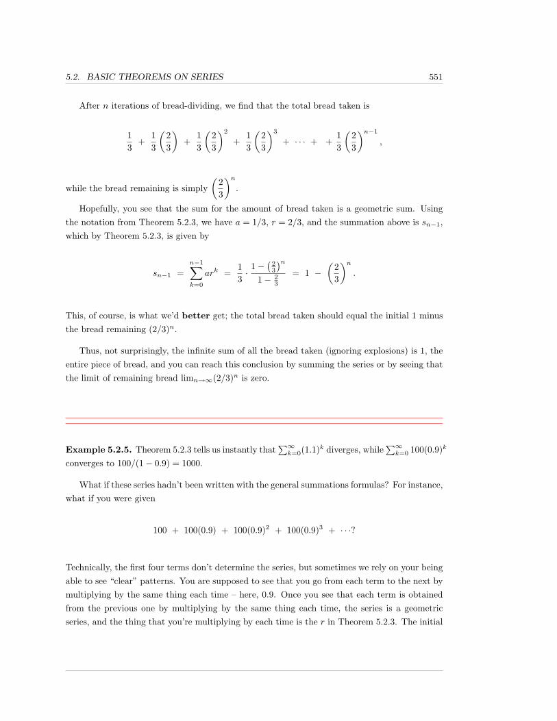
5.2. BASIC THEOREMS ON SERIES 551
After n iterations of bread-dividing, we find that the total bread taken is
13
+13
(23
)+
13
(23
)2
+13
(23
)3
+ · · · + +13
(23
)n−1
,
while the bread remaining is simply(
23
)n.
Hopefully, you see that the sum for the amount of bread taken is a geometric sum. Usingthe notation from Theorem 5.2.3, we have a = 1/3, r = 2/3, and the summation above is sn−1,which by Theorem 5.2.3, is given by
sn−1 =n−1∑k=0
ark =13·
1−(
23
)n1− 2
3
= 1 −(
23
)n.
This, of course, is what we’d better get; the total bread taken should equal the initial 1 minusthe bread remaining (2/3)n.
Thus, not surprisingly, the infinite sum of all the bread taken (ignoring explosions) is 1, theentire piece of bread, and you can reach this conclusion by summing the series or by seeing thatthe limit of remaining bread limn→∞(2/3)n is zero.
Example 5.2.5. Theorem 5.2.3 tells us instantly that∑∞k=0(1.1)k diverges, while
∑∞k=0 100(0.9)k
converges to 100/(1− 0.9) = 1000.
What if these series hadn’t been written with the general summations formulas? For instance,what if you were given
100 + 100(0.9) + 100(0.9)2 + 100(0.9)3 + · · ·?
Technically, the first four terms don’t determine the series, but sometimes we rely on your beingable to see “clear” patterns. You are supposed to see that you go from each term to the next bymultiplying by the same thing each time – here, 0.9. Once you see that each term is obtainedfrom the previous one by multiplying by the same thing each time, the series is a geometricseries, and the thing that you’re multiplying by each time is the r in Theorem 5.2.3. The initial
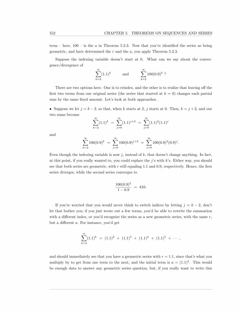
552 CHAPTER 5. THEOREMS ON SEQUENCES AND SERIES
term – here, 100 – is the a in Theorem 5.2.3. Now that you’ve identified the series as beinggeometric, and have determined the r and the a, you apply Theorem 5.2.3.
Suppose the indexing variable doesn’t start at 0. What can we say about the conver-gence/divergence of
∞∑k=2
(1.1)k and∞∑k=2
100(0.9)k ?
There are two options here. One is to reindex, and the other is to realize that leaving off thefirst two terms from our original series (the series that started at k = 0) changes each partialsum by the same fixed amount. Let’s look at both approaches.
• Suppose we let j = k− 2, so that, when k starts at 2, j starts at 0. Then, k = j + 2, and ourtwo sums become
∞∑k=2
(1.1)k =∞∑j=0
(1.1)j+2 =∞∑j=0
(1.1)2(1.1)j
and∞∑k=2
100(0.9)k =∞∑j=0
100(0.9)j+2 =∞∑j=0
100(0.9)2(0.9)j .
Even though the indexing variable is now j, instead of k, that doesn’t change anything. In fact,at this point, if you really wanted to, you could replace the j’s with k’s. Either way, you shouldsee that both series are geometric, with r still equaling 1.1 and 0.9, respectively. Hence, the firstseries diverges, while the second series converges to
100(0.9)2
1− 0.9= 810.
If you’re worried that you would never think to switch indices by letting j = k − 2, don’tlet that bother you; if you just wrote out a few terms, you’d be able to rewrite the summationwith a different index, or you’d recognize the series as a new geometric series, with the same r,but a different a. For instance, you’d get
∞∑k=2
(1.1)k = (1.1)2 + (1.1)3 + (1.1)4 + (1.1)5 + · · · ,
and should immediately see that you have a geometric series with r = 1.1, since that’s what youmultiply by to get from one term to the next, and the initial term is a = (1.1)2. This wouldbe enough data to answer any geometric series question, but, if you really want to write this
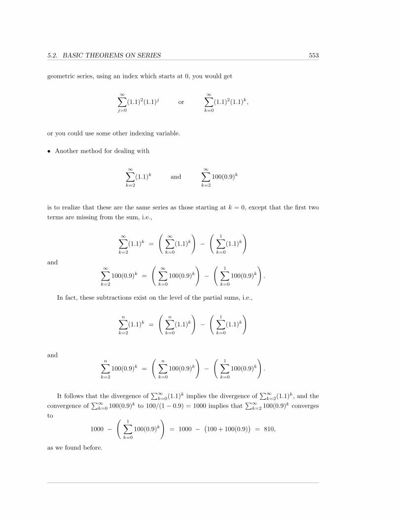
5.2. BASIC THEOREMS ON SERIES 553
geometric series, using an index which starts at 0, you would get
∞∑j=0
(1.1)2(1.1)j or∞∑k=0
(1.1)2(1.1)k,
or you could use some other indexing variable.
• Another method for dealing with
∞∑k=2
(1.1)k and∞∑k=2
100(0.9)k
is to realize that these are the same series as those starting at k = 0, except that the first twoterms are missing from the sum, i.e.,
∞∑k=2
(1.1)k =
( ∞∑k=0
(1.1)k)−
(1∑k=0
(1.1)k)
and∞∑k=2
100(0.9)k =
( ∞∑k=0
100(0.9)k)−
(1∑k=0
100(0.9)k).
In fact, these subtractions exist on the level of the partial sums, i.e.,
n∑k=2
(1.1)k =
(n∑k=0
(1.1)k)−
(1∑k=0
(1.1)k)
andn∑k=2
100(0.9)k =
(n∑k=0
100(0.9)k)−
(1∑k=0
100(0.9)k).
It follows that the divergence of∑∞k=0(1.1)k implies the divergence of
∑∞k=2(1.1)k, and the
convergence of∑∞k=0 100(0.9)k to 100/(1 − 0.9) = 1000 implies that
∑∞k=2 100(0.9)k converges
to
1000 −
(1∑k=0
100(0.9)k)
= 1000 −(100 + 100(0.9)
)= 810,
as we found before.
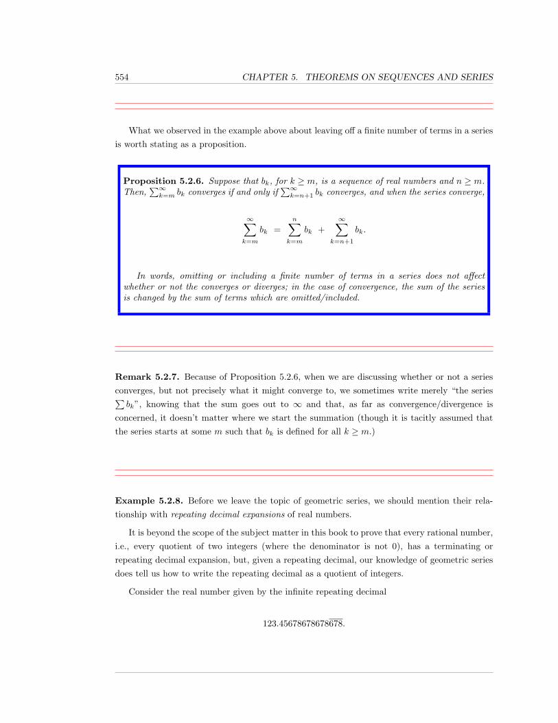
554 CHAPTER 5. THEOREMS ON SEQUENCES AND SERIES
What we observed in the example above about leaving off a finite number of terms in a seriesis worth stating as a proposition.
Proposition 5.2.6. Suppose that bk, for k ≥ m, is a sequence of real numbers and n ≥ m.Then,
∑∞k=m bk converges if and only if
∑∞k=n+1 bk converges, and when the series converge,
∞∑k=m
bk =n∑
k=m
bk +∞∑
k=n+1
bk.
In words, omitting or including a finite number of terms in a series does not affectwhether or not the converges or diverges; in the case of convergence, the sum of the seriesis changed by the sum of terms which are omitted/included.
Remark 5.2.7. Because of Proposition 5.2.6, when we are discussing whether or not a seriesconverges, but not precisely what it might converge to, we sometimes write merely “the series∑bk”, knowing that the sum goes out to ∞ and that, as far as convergence/divergence is
concerned, it doesn’t matter where we start the summation (though it is tacitly assumed thatthe series starts at some m such that bk is defined for all k ≥ m.)
Example 5.2.8. Before we leave the topic of geometric series, we should mention their rela-tionship with repeating decimal expansions of real numbers.
It is beyond the scope of the subject matter in this book to prove that every rational number,i.e., every quotient of two integers (where the denominator is not 0), has a terminating orrepeating decimal expansion, but, given a repeating decimal, our knowledge of geometric seriesdoes tell us how to write the repeating decimal as a quotient of integers.
Consider the real number given by the infinite repeating decimal
123.45678678678678.
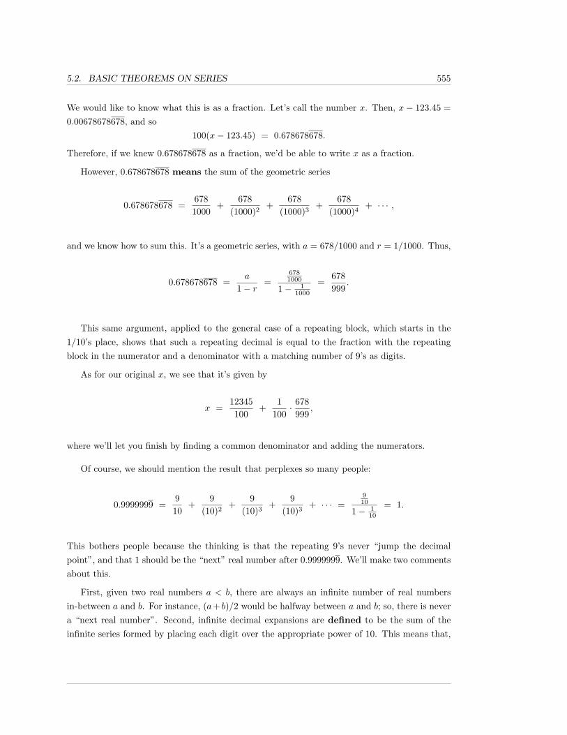
5.2. BASIC THEOREMS ON SERIES 555
We would like to know what this is as a fraction. Let’s call the number x. Then, x− 123.45 =0.00678678678, and so
100(x− 123.45) = 0.678678678.
Therefore, if we knew 0.678678678 as a fraction, we’d be able to write x as a fraction.
However, 0.678678678 means the sum of the geometric series
0.678678678 =6781000
+678
(1000)2+
678(1000)3
+678
(1000)4+ · · · ,
and we know how to sum this. It’s a geometric series, with a = 678/1000 and r = 1/1000. Thus,
0.678678678 =a
1− r=
6781000
1− 11000
=678999
.
This same argument, applied to the general case of a repeating block, which starts in the1/10’s place, shows that such a repeating decimal is equal to the fraction with the repeatingblock in the numerator and a denominator with a matching number of 9’s as digits.
As for our original x, we see that it’s given by
x =12345100
+1
100· 678
999,
where we’ll let you finish by finding a common denominator and adding the numerators.
Of course, we should mention the result that perplexes so many people:
0.9999999 =910
+9
(10)2+
9(10)3
+9
(10)3+ · · · =
910
1− 110
= 1.
This bothers people because the thinking is that the repeating 9’s never “jump the decimalpoint”, and that 1 should be the “next” real number after 0.9999999. We’ll make two commentsabout this.
First, given two real numbers a < b, there are always an infinite number of real numbersin-between a and b. For instance, (a+ b)/2 would be halfway between a and b; so, there is nevera “next real number”. Second, infinite decimal expansions are defined to be the sum of theinfinite series formed by placing each digit over the appropriate power of 10. This means that,
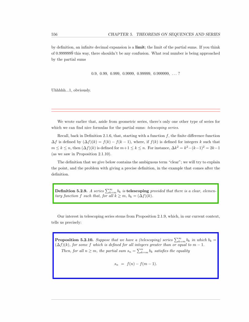
556 CHAPTER 5. THEOREMS ON SEQUENCES AND SERIES
by definition, an infinite decimal expansion is a limit; the limit of the partial sums. If you thinkof 0.9999999 this way, there shouldn’t be any confusion. What real number is being approachedby the partial sums
0.9, 0.99, 0.999, 0.9999, 0.99999, 0.999999, . . . ?
Uhhhhh...1, obviously.
We wrote earlier that, aside from geometric series, there’s only one other type of series forwhich we can find nice formulas for the partial sums: telescoping series.
Recall, back in Definition 2.1.6, that, starting with a function f , the finite difference function∆f is defined by (∆f)(k) = f(k) − f(k − 1), where, if f(k) is defined for integers k such thatm ≤ k ≤ n, then (∆f)(k) is defined for m+1 ≤ k ≤ n. For instance, ∆k2 = k2−(k−1)2 = 2k−1(as we saw in Proposition 2.1.10).
The definition that we give below contains the ambiguous term “clear”; we will try to explainthe point, and the problem with giving a precise definition, in the example that comes after thedefinition.
Definition 5.2.9. A series∑∞k=m bk is telescoping provided that there is a clear, elemen-
tary function f such that, for all k ≥ m, bk = (∆f)(k).
Our interest in telescoping series stems from Proposition 2.1.9, which, in our current context,tells us precisely:
Proposition 5.2.10. Suppose that we have a (telescoping) series∑∞k=m bk in which bk =
(∆f)(k), for some f which is defined for all integers greater than or equal to m− 1.Then, for all n ≥ m, the partial sum sn =
∑nk=m bk satisfies the equality
sn = f(n)− f(m− 1).
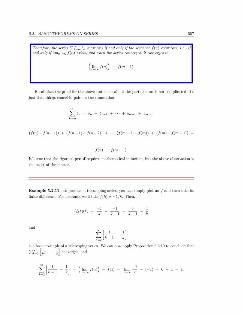
5.2. BASIC THEOREMS ON SERIES 557
Therefore, the series∑∞k=m bk converges if and only if the sequence f(n) converges, i.e., if
and only if limn→∞ f(n) exists, and when the series converges, it converges to
(limn→∞
f(n))− f(m− 1).
Recall that the proof for the above statement about the partial sums is not complicated; it’sjust that things cancel in pairs in the summation:
n∑k=m
bk = bn + bn−1 + · · · + bm+1 + bm =
(f(n)− f(n− 1)
)+(f(n− 1)− f(n− 2)
)+ · · ·
(f(m+ 1)− f(m)
)+(f(m)− f(m− 1)
)=
f(n) − f(m− 1).
It’s true that the rigorous proof requires mathematical induction, but the above observation isthe heart of the matter.
Example 5.2.11. To produce a telescoping series, you can simply pick an f and then take itsfinite difference. For instance, we’ll take f(k) = −1/k. Then,
(∆f)(k) =−1k− −1
k − 1=
1k − 1
− 1k
and∞∑k=2
[1
k − 1− 1
k
]is a basic example of a telescoping series. We can now apply Proposition 5.2.10 to conclude that∑∞k=2
[1
k−1 −1k
]converges, and
∞∑k=2
[1
k − 1− 1
k
]=(
limn→∞
f(n))− f(1) = lim
n→∞
−1n− (−1) = 0 + 1 = 1.
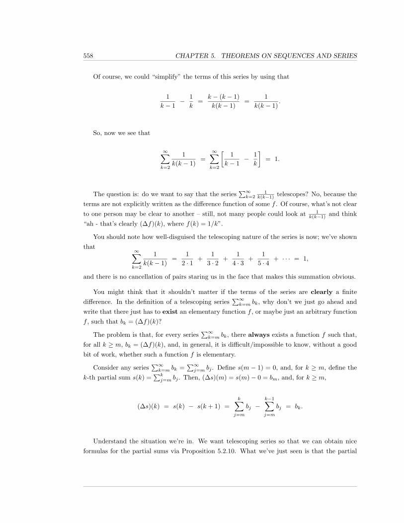
558 CHAPTER 5. THEOREMS ON SEQUENCES AND SERIES
Of course, we could “simplify” the terms of this series by using that
1k − 1
− 1k
=k − (k − 1)k(k − 1)
=1
k(k − 1).
So, now we see that
∞∑k=2
1k(k − 1)
=∞∑k=2
[1
k − 1− 1
k
]= 1.
The question is: do we want to say that the series∑∞k=2
1k(k−1) telescopes? No, because the
terms are not explicitly written as the difference function of some f . Of course, what’s not clearto one person may be clear to another – still, not many people could look at 1
k(k−1) and think“ah - that’s clearly (∆f)(k), where f(k) = 1/k”.
You should note how well-disguised the telescoping nature of the series is now; we’ve shownthat
∞∑k=2
1k(k − 1)
=1
2 · 1+
13 · 2
+1
4 · 3+
15 · 4
+ · · · = 1,
and there is no cancellation of pairs staring us in the face that makes this summation obvious.
You might think that it shouldn’t matter if the terms of the series are clearly a finitedifference. In the definition of a telescoping series
∑∞k=m bk, why don’t we just go ahead and
write that there just has to exist an elementary function f , or maybe just an arbitrary functionf , such that bk = (∆f)(k)?
The problem is that, for every series∑∞k=m bk, there always exists a function f such that,
for all k ≥ m, bk = (∆f)(k), and, in general, it is difficult/impossible to know, without a goodbit of work, whether such a function f is elementary.
Consider any series∑∞k=m bk =
∑∞j=m bj . Define s(m − 1) = 0, and, for k ≥ m, define the
k-th partial sum s(k) =∑kj=m bj . Then, (∆s)(m) = s(m)− 0 = bm, and, for k ≥ m,
(∆s)(k) = s(k) − s(k + 1) =k∑
j=m
bj −k−1∑j=m
bj = bk.
Understand the situation we’re in. We want telescoping series so that we can obtain niceformulas for the partial sums via Proposition 5.2.10. What we’ve just seen is that the partial
5.2. BASIC THEOREMS ON SERIES 559
sums yield a function which tells us that any series telescopes, but, if we use the partial sumfunction for the telescoping, we arrive at the useless result that knowing the partial sums wouldenable us to determine the partial sums. Hence, we need to put some restrictions on the type,or clarity, of the function f that we’re allowed to choose such that bk = (∆f)(k).
The point is, in order for Proposition 5.2.10 to be useful, the function f needs to be man-ageable, i.e., elementary, and it needs to be easily discernible.
One of the things that we just saw in the previous example leads us to an interesting result,a result that can tell us that there’s an easy way to see that some series diverge.
Suppose that have a series∑∞k=m bk, and it converges to L. If we let sn be the partial
sum sn =∑nk=m bk, then, as we saw in the example above, bn = sn − sn−1. However, as the
series converges to L, the partial sums converge to L, and so limn→∞ sn = limn→∞ sn−1 = L.Therefore,
limn→∞
bn = limn→∞
(sn − sn−1) = limn→∞
sn − limn→∞
sn−1 = L− L = 0.
Thus, if a series converges, then the terms must approach 0. This is usually used in the logicallyequivalent, contrapositive, form, which we state first.
Theorem 5.2.12. (Term Test for Divergence)
1. If the terms of a series do not approach 0, then the series diverges.
2. Equivalently, if a series converges, then the terms must approach 0.
3. If the terms of a series approach 0, the series may either converge or diverge, i.e., youcan conclude nothing merely from the fact that the terms approach 0.
Item 2 of the Term Test tells us that any convergent series must have its terms approach 0;so that every convergent series that we’ve discussed so far, like the alternating harmonic seriesor geometric series with |r| < 1, are examples of convergent series for which the terms approach0. However, we have mentioned before the harmonic series,
∞∑k=1
1k
= 1 +12
+13
+14
+ · · · ,
560 CHAPTER 5. THEOREMS ON SEQUENCES AND SERIES
which is a fundamental example of a series in which the terms approach 0, and yet the seriesstill diverges. We will show that the harmonic series diverges in Proposition 5.2.16, after wegive some easy examples of using the Term Test for Divergence. But what’s going on? How cana series diverge if the terms approach 0?
The point of the harmonic series example is to show that it’s not enough for the terms
of a series to approach 0 in order to conclude convergence of the series; the terms
need to approach 0 fast enough to make up for the fact that we’re adding more and
more of them together.
The reason that the Term Test is called the Term Test for Divergence is that the test tellsyou that some series diverge, but it can NEVER tell you, by itself, that a series converges.
Example 5.2.13. Consider the series
∞∑k=1
(14
+7k
).
As k →∞, the terms14
+7k
approach14
, not 0. Therefore, the series diverges by the Term Testfor Divergence, Theorem 5.2.12.
Understand what’s going on here: the sequence of terms converges, and what the termsconverge to is 1/4, but the value of the series is what you get when you add together an infinitenumber of terms, so, basically, in the series, it’s as though you’re adding together an infinite
number of 1/4’s; not surprisingly, this adds up to ∞, and so the series diverges to ∞.
It is a fundamental error to confuse the limit of the terms with the sum of the series. Thesum of the series is absolutely not the limit of the terms. The terms are what are beingadded in the series. The sum of the series is the limit of the partial sums, which is thuswhat is approached as you add more and more terms.
Example 5.2.14. What does the Term Test for Divergence tell us about the convergence ordivergence of
∞∑k=1
7k
?
5.2. BASIC THEOREMS ON SERIES 561
It is tempting to say “ah – now the terms approach 0, so the series must converge, by the TermTest for Divergence”.
But remember Item 3 of the Term Test of Divergence; you can conclude nothing about theconvergence or divergence of the series when the terms approach 0.
In fact, the series∑∞k=1
7k is, term-wise, 7 times the harmonic series, and so, like the harmonic
series, it diverges.
Example 5.2.15. What about the series∞∑k=0
(−1)k?
Here, the limit of the terms does not exist, since, as k gets bigger, (−1)k continues to alternatebetween −1 and 1. Does the Term Test for Divergence tell us anything about this series?
Yes - if the limit of the terms fails to exist, then it is true that “the terms of the series do notapproach 0”; in fact, the terms don’t approach anything, so, in particular, they don’t approach0. Hence, the series
∑∞k=0(−1)k diverges by the Term Test for Divergence.
We have put it off long enough. We are going to show that the harmonic series diverges. Infact, this will follow, as a special case of our p-series Test, Corollary 5.3.15, but we give a morebasic argument here because it is instructive.
Proposition 5.2.16. The harmonic series
∞∑k=1
1k
= 1 +12
+13
+14
+ · · · (5.1)
diverges to ∞.
Proof. We want to show that, as n→∞, the sequence of partial sums
Sn =n∑k=1
1k
562 CHAPTER 5. THEOREMS ON SEQUENCES AND SERIES
goes to ∞.
Note that, as each partial sum is obtained from earlier partial sums by adding positive terms,the sequence of partial sums Sn is increasing. Therefore, by Theorem 5.1.23, the sequence Sndiverges if and only if the sequence is unbounded.
We shall find a lower bound on some of the partial sums, the partial sums of the form S2p ,and show that this lower bound approaches ∞, which forces the harmonic series to diverge.Technically, we should use mathematical induction, but we’ll make the idea clear.
The “trick” is to group together collections of terms in such a way that each group clearlyadds up to something greater than 1/2. We will indicate the groups with parentheses:
(1)+(
12
)+(
13
+14
)+(
15
+16
+17
+18
)+(
19
+110
+111
+112
+113
+114
+115
+116
)+· · · .
You always end a group at 1 over a power of 2, and start the group at 1 over the next numberafter the last power of 2. Notice that, in each group, all of the summands are greater than orequal to the last one in that group. So that, what we’ve written above is clearly greater thanor equal to
1 +12
+ 2 · 14
+ 4 · 18
+ 8 · 116
+ · · · = 1 +12
+12
+12
+12
+ · · · .
Thus, what we find is that, for each p ≥ 1,
S2p ≥ 1 +p
2.
As p → ∞, 1 + p2 → ∞, and thus S2p → ∞. Therefore, the increasing sequence of partial
sums is unbounded and approaches ∞.
The harmonic series should be an example that you always keep in mind. It’s the most basicexample of a series in which the terms approach 0, and yet the series nonetheless diverges.This shows that you cannot conclude convergence of a series simply because the termsapproach 0.
5.2. BASIC THEOREMS ON SERIES 563
Multiplying a series by a constant, and adding two series works as you’d expect. The proofsusing limits of partial sums are straightforward; we leave them for you as an exercise.
Theorem 5.2.17. Suppose that we have infinite series∑∞k=m ak and
∑∞k=m bk.
1. Assume that c 6= 0. Then, the series∑∞k=m ak converges if and only if the series∑∞
k=m cak converges and, when the series converge,
∞∑k=m
cak = c ·∞∑k=m
ak.
2. Suppose that∑∞k=m ak converges. Then,
∑∞k=m bk converges if and only if
∑∞k=m(ak+
bk) converges and, when the series converge,
∞∑k=m
(ak + bk) =∞∑k=m
ak +∞∑k=m
bk.
By letting c = −1 in Item 1 above, and combining with Item 2, you can, naturally, obtainan analogous result about subtracting one series from another.
Example 5.2.18. By Theorem 5.2.3, the series∑∞k=2
(13
)k converges and, by Remark 4.4.13and Proposition 5.2.6, the series
∑∞k=2(−1)k−1
(1k
)also converges (it’s the alternating harmonic
series, except that the first term is missing). In fact, we know what these series converge to:
∞∑k=2
(13
)k=
[ ∞∑k=0
(13
)k]− 1− 1
3=
11− 1
3
− 43
=16,
and∞∑k=2
(−1)k−1
(1k
)=
[ ∞∑k=1
(−1)k−1
(1k
)]− 1 = (ln 2)− 1.
564 CHAPTER 5. THEOREMS ON SEQUENCES AND SERIES
Thus, Theorem 5.2.17 tells us that
∞∑k=2
[6(
13
)k+ (−1)k
(1k
)]=
∞∑k=2
[6(
13
)k− (−1)k−1
(1k
)]=
6 ·∞∑k=2
(13
)k−
∞∑k=2
(−1)k−1
(1k
)= 6 · 1
6−((ln 2)− 1
)= 2− ln 2.
Example 5.2.19. You need to be careful not to try to apply Theorem 5.2.17 to sums of twodivergent series. The term-by-term sum of two divergent series may diverge or converge.
For instance, the harmonic series∑∞k=1
1k diverges. If you take the harmonic series, and add
it to itself term-wise, you get∞∑k=1
(1k
+1k
)=
∞∑k=1
2k,
which diverges by Item 1 of Theorem 5.2.17, since it’s 2 times the harmonic series (in the term-wise sense). What this shows is that the term-by-term sum of two divergent series may againbe divergent.
On the other hand, using Item 1 of Theorem 5.2.17 with c = −1, we conclude that∑∞k=1
(− 1k
)diverges. But the term-wise sum of
∑∞k=1
1k and
∑∞k=1
(− 1k
)is
∞∑k=1
[1k− 1k
]=
∞∑k=1
0 = 0,
so that the term-wise sum of these two divergent series converges to 0.
The point is that the term-by-term sum of two divergent series may converge or may diverge.There is no theorem that quickly tells you what happens.
However, you may correctly suspect that the above example of two divergent series beingadded, term-wise, and producing a convergent series can happen only because of cancellation.If all of the terms of both series had been ≥ 0, or all of the terms of both series had been ≤ 0,then the term-by-term sum of two divergent series would again be divergent. We will see thisin the next section.
5.2. BASIC THEOREMS ON SERIES 565
In the example above, we saw that standard algebraic operations may not work so well whendealing with divergent series. Actually, things may be worse than you suspect.
Suppose that we have a series
∞∑k=m
ak = am + am+1 + am+2 + am+3 + am+4 + am+5 + · · · .
Since addition is associative, you might suspect that we can throw in parentheses anywhere thatwe want and not change the sum. However, if the series diverges, it is not true that groupingthe terms necessarily leads to a series that continues to diverge.
Example 5.2.20. Consider the series
1 − 1 + 1 − 1 + 1 − 1 + · · · .
We write this summation without any parentheses, because we assume that it’s obvious thatwe mean the series
∑∞k=1(−1)k−1. This series diverges by the Term Test for Divergence, Theo-
rem 5.2.12; the terms do not approach 0. However, you’re so used to the associativity of additionthat you might believe that this series is the same as
(1 − 1) + (1 − 1) + (1 − 1) + · · ·
or
1 + (− 1 + 1) + (− 1 + 1) + (− 1 + 1) + · · · ,
but these latter two series converge to 0 and 1, respectively, assuming that the groupings indicatethe terms of the series. Thus, it is possible to start with a divergent series and, by groupingsome terms together to form a new series, arrive at convergent series, and it’s possible to getconvergent series which converge to different numbers.
However, for convergent series, “associativity” works as you would expect.
566 CHAPTER 5. THEOREMS ON SEQUENCES AND SERIES
Theorem 5.2.21. Suppose that the terms of a series∑∞j=n bj are formed from a convergent
series∑∞k=m ak by grouping disjoint finite sums of the ak without changing the order, i.e.,
suppose that the series∑∞j=n bj is formed by “adding some parentheses” to the convergent
series∑∞k=m ak.
Then,∑∞j=n bj converges, and
∞∑j=n
bj =∞∑k=m
ak.
Proof. The partial sums of∑∞j=n bj are sums of the ak’s, in order, and so form a subsequence
of the sequence of partial sums of∑∞k=m ak, which we are assuming is a convergent sequence.
Theorem 5.1.27 immediately yields the theorem.
As we shall see in the next section, if all of the terms in a series are non-negative, it is not
possible to group a divergent series in such a way that you get a convergent series; that is, theweird thing that happened in Example 5.2.20 can’t happen if all of the terms in the series arenon-negative.
5.2.1 Exercises
In each of Exercises 1 through 10, list the first 5 terms of the series, and the first
5 partial sums. Give the partial sums written out as summations, and (possibly
using a calculator), also give each partial sum as a single number.
1.11
+14
+17
+110
+113
+116
+119
+ · · ·
2.11− 1
5+
110− 1
15+
120− 1
25+
130
+ · · ·
3.∞∑k=0
(−2)k
4.∞∑k=0
(−1
2
)k
5.∞∑k=1
[1k2− 1
(k + 1)2
]
5.2. BASIC THEOREMS ON SERIES 567
6.∞∑j=1
j
j3 + 1
7.∞∑
p=−3
p2
8.∞∑
p=−3
(−1)pp2
9.∞∑n=4
2n− 3
10.∞∑
k=−2
2k + 3
In each of Exercises 11 through 20, you are given m and a formula for the partial
sum sn =∑ni=m bi of an infinite series
∑∞i=m bi. (a) Give the terms bm, . . . , bm+4, (b)
give a formula for the general term bi, and (c) determine whether the series∑∞i=m bi
converges or diverges; if it converges, determine what it converges to.
11. sn =1n
, m = 1
12. sn = 1− 1n
, m = 1
13. sn = (−1)n, m = 0
14. sn = 1, m = 0
15. sn = 2 +n
en, m = 0
16. sn =5√n
, m = 1
17. sn =1
(n− 2)(n− 1), m = 3
18. sn = ln(5n2)− ln(n2 + 1), m = 1
19. sn =2n+ 3n
, m = 1
20. sn =2n
n!, m = 1
568 CHAPTER 5. THEOREMS ON SEQUENCES AND SERIES
In each of Exercises 21 through 30, you are given a series which is geometric,
telescopic, or diverges by the Term Test for Divergence, Theorem 5.2.12. Determine
if the series converges or diverges; if it converges, determine what it converges to.
21.∞∑k=1
[1 +
1k
]
22.∞∑k=1
[1
k + 1− 1k
]
23.∞∑k=1
(1 +
1k
)k
24.∞∑j=0
75j
25.∞∑j=0
(75
)j
26.∞∑j=0
(57
)j
27.∞∑j=0
(−5
7
)j
28.∞∑p=1
[(p+ 1)2 − p2
]
29.∞∑q=1
[tan−1(q)− tan−1(q + 1)
]
30.∞∑q=1
tan−1(q)
In each of Exercise 31 through 40, determine if the given series converges or di-
verges. If it converges, determine what it converges to.
31.∞∑k=1
[(1k− 1k + 1
)+
5(−1)k
3k
]
32.∞∑p=1
110p
5.2. BASIC THEOREMS ON SERIES 569
33.∞∑p=1
(−1)p
10p
34.∞∑j=1
[1j
+5(−1)j
3j
]
35.∞∑r=0
[27r
+5(−1)r
3r
]
36.∞∑r=0
[r
7+
5(−1)r
3r
]
37.∞∑k=1
[k − 1k
+32k
]
38.∞∑k=1
[32k
+ 5(
sin(
1k
)− sin
(1
k + 1
))]
39.∞∑k=1
[−74k
+ 5((k + 1)2 − k2
)]
40.∞∑k=0
[3
2k7+
13k100
]
In each of Exercise 41 through 44, write the repeating decimal as a quotient of
positive integers.
41. 0.2301230123012301
42. 0.141572727272
43. 2.71828182818281
44. 123.123123123
45. Suppose that∑∞k=1 ak = 7 and
∑∞k=1 bk = −2. What can you conclude about the series∑∞
k=1(2ak − 3bk)?
46. Suppose that∑∞k=1 ak = 3 and
∑∞k=1 bk = −3. What can you conclude about the series∑∞
k=1(2ak − 3bk)?
47. Suppose that∑∞k=1 ak = 7 and
∑∞k=1 bk diverges. What can you conclude about the series∑∞
k=1(2ak − 3bk)?
570 CHAPTER 5. THEOREMS ON SEQUENCES AND SERIES
48. Suppose that∑∞k=1 ak diverges and
∑∞k=1 bk diverges. What can you conclude about the
series∑∞k=1(2ak − 3bk)?
49. Consider the series
∞∑k=0
ak =32− 1 +
54− 1 +
98− 1 +
1716− 1 + · · · ,
in which, for all n ≥ 0, a2n = (2n+1 + 1)/2n+1 and a2n+1 = −1.
a. Show that the series diverges.
b. By grouping terms together, i.e., by inserting parentheses into the summation, showthat you can obtain a convergent series.
50. Consider the series∞∑k=1
[(−1)k +
1k2
].
a. Show that the series diverges.
b. By grouping terms together, i.e., by inserting parentheses into the summation, showthat you can obtain a convergent series.
51. Explain why the harmonic series is an important example, i.e., what it is an importantexample of.
52. Prove that the “even harmonic series”∞∑k=1
12k
diverges.
53. Prove that the “odd harmonic series”∞∑k=0
12k + 1
diverges.
54. Prove Theorem 5.2.17, on multiplying series by constants and adding two series.
55. A man is jogging home, accompanied by his dog. The man is a mile from home, and jogsat a constant speed of 5 miles per hour. His dog runs in front of him at a constant speedof 10 miles per hour and, when the dog gets home, he turns around and runs, at 10 mph,back to the man. When the dog reaches the man, the dog turns around and runs homeagain, at 10 mph. The dog continues running home and returning the man, at 10 mph,for the entire time it takes for the man to jog home. Assume that the time it takes thedog to turn around is negligible, so that the dog is really running at 10 mph for the wholetrip.
a. Write an infinite series for the total distance traveled by the dog. Your series shouldhave as terms the distance traveled by the dog during each leg of his trip.

5.2. BASIC THEOREMS ON SERIES 571
b. Sum the series from part (a).
c. Use a simple distance/speed/time argument to obtain the same answer that youobtained in part (b).
572 CHAPTER 5. THEOREMS ON SEQUENCES AND SERIES
5.3 Theorems on Series II:Non-negative Series
Series in which all of the terms are greater than or equal to zero, non-negative series, or inwhich all of the terms are less than or equal to zero, non-positive series, are easier to dealwith than series that contain both positive and negative terms. However, all of the results onconvergence/divergence for non-positive series can be obtained by negating, term-by-term, toobtain non-negative series, and then looking at the results for non-negative series. Consequently,it is customary to state the results, the convergence and divergence tests, for non-negative seriesonly, leaving the results for non-positive series as quick corollaries.
Non-negative series are more manageable than series with both positive and negative termsbecause, for a non-negative series, the sequence of partial sums is increasing, and Theorem 5.1.23then tells us that the sequence of partial sums converges, i.e., the series converges, if and onlyif the sequence of partial sums is bounded above.
This will allow us to derive three useful tests for convergence of non-negative series: theIntegral Test, the Comparison test, and the Limit Comparison Test.
Definition 5.3.1. A series∑∞k=m bk is non-negative provided that, for all k ≥ m, bk ≥ 0.
Example 5.3.2. A geometric series∑∞k=0 ar
k is non-negative if and only if a ≥ 0 and r ≥ 0.
The harmonic series∑∞k=1
1k is non-negative, while the alternating harmonic series
∑∞k=1(−1)k−1 1
k
is not non-negative (nor is it non-positive).
The series
∞∑k=1
(1 + sin
(kπ
2
))(1k
)= 2 · 1 + 1 · 1
2+ 0 · 1
3+ 1 · 1
4+ 2 · 1
5+ 1 · 1
6+ 0 · 1
7+ · · ·
is non-negative, even though there are an infinite number of terms which equal 0.
5.3. NON-NEGATIVE SERIES 573
From the definition of a non-negative series, the sequence of partial sums of a non-negativeseries is increasing and so, from Theorem 5.1.23, we immediately conclude:
Theorem 5.3.3. The partial sums of a non-negative series are an increasing sequence and,consequently, a non-negative series converges if and only if the partial sums are boundedabove; if the partial sums are bounded above by M , then the sum of the convergent series is≤M . A non-negative series diverges if and only if it diverges to ∞.
Recall the definition of a subsequence in Definition 5.1.26. If we have a series∑∞n=m an
(non-negative or not), and form a new series by using as terms a subsequence of the an, we referto this new series as a subseries.
Now, if we have a non-negative series∑∞n=m an, then the partial sums of any subseries are
less than or equal to partial sums from∑∞n=m an itself. Therefore, Theorem 5.3.3 immediately
yields the following corollary.
Corollary 5.3.4. Suppose that∑∞n=m an is a non-negative series which converges. Then,
every subseries of∑∞n=m an converges.
In other words, if a subseries of a non-negative series diverges (necessarily to ∞), thenthe original series also diverges to ∞.
Example 5.3.5. Consider the last non-negative series from Example 5.3.2:
∞∑k=1
(1 + sin
(kπ
2
))(1k
)= 2 · 1 + 1 · 1
2+ 0 · 1
3+ 1 · 1
4+ 2 · 1
5+ 1 · 1
6+ 0 · 1
7+ · · · .
If we consider the subseries using those terms where k is even, we obtain
1 · 12
+ 1 · 14
+ 1 · 16
+ + 1 · 18
+ · · · =∞∑j=1
12· 1j,
which is, term-wise, 1/2 of the harmonic series. Thus, by Theorem 5.2.17,∑∞j=1
12 ·
1j diverges
and by Corollary 5.3.4, so does the original series∑∞k=1
(1 + sin
(kπ2
)) (1k
).
574 CHAPTER 5. THEOREMS ON SEQUENCES AND SERIES
Example 5.3.6. The conclusion of Corollary 5.3.4 is not true (in general) if we omit thecondition that the series is non-negative. Consider the alternating harmonic series,
1 − 12
+13− 1
4+
15− 1
6+ · · · ,
which, as we discussed in Remark 4.4.13, converges to ln 2. However, if you just add up allof the negative terms, the terms with even denominators, you get, term-wise, −1/2 times theharmonic series, which diverges.
Thus, series that contain both positive and negative terms may converge, even though sub-series may diverge.
Recall that Theorem 5.2.21 told us that grouping together sums in a convergent series hasno effect on the convergence. In Example 5.2.20, we saw a divergent series that contains bothpositive and negative terms, for which it is possible to group the terms to form new series thatconverge. As another corollary to Theorem 5.3.3, we will now show that you cannot group thesummations in a divergent non-negative series in order to produce a convergent series.
Corollary 5.3.7. Suppose that the terms of a series∑∞j=n bj are formed from a divergent
non-negative series∑∞k=m ak by grouping disjoint finite sums of the ak without changing the
order, i.e., by “adding some parentheses” to the divergent series∑∞k=m ak.
Then,∑∞j=n bj also diverges.
Proof. Each partial sum of∑∞j=n bj is also a partial sum of
∑∞k=m ak, and the partial sums of∑∞
k=m ak diverge to ∞. Therefore, the partial sums of∑∞j=n bj also diverge to ∞.
Now that we know, from Theorem 5.2.21 and Corollary 5.3.7, that grouping terms (i.e.,inserting parentheses around finite numbers of terms) does not affect the convergence or diver-gence of a non-negative series, we would like to know that changing the order of the summation,i.e., rearranging the order in which the terms are added, also does not affect non-negative series.
For instance, we know that
112
+122
+132
+142
+152
+162
+ · · ·
5.3. NON-NEGATIVE SERIES 575
converges and, in fact, we stated that it converges to π2/6. Does it follow that the series formedby switching pairs of terms,
122
+112
+142
+132
+162
+152
+ · · · , (5.2)
converges, and converges to π2/6? You might think “sure - a sum doesn’t care what order youadd things in”, and that’s true for finite sums, but, as we shall see in the next section, it is false,in general, for series containing both positive and negative terms. However, non-negative seriesare well-behaved with respect to such rearrangements.
First, we need to give the technical definition of a rearrangement. Note that the only thingthat we really need to rearrange is the order of the indices of the sequence of terms. For instance,if we let ak = 1/k2, then the series in Formula 5.2 is
a2 + a1 + a4 + a3 + a6 + a5 + · · · .
Suppose that, for all integers j ≥ 1, we define r(j) = j + 1 if j is odd, and r(j) = j − 1 if j iseven. Then,
r(1) = 2, r(2) = 1, r(3) = 4, r(4) = 3, r(5) = 6, r(6) = 5, · · · .
Then, the series in Formula 5.2 is simply∑∞k=1 br(k). All that we used here to reorder, or
rearrange, our series was the one-to-one correspondence (the bijection) r between the originalindices and the newly ordered indices.
Definition 5.3.8. Consider a (not necessarily non-negative) series∑∞k=m bk.
A permutation of the indices of the series is a one-to-one correspondence, a bijection,r : Z≥m → Z≥m.
A rearrangement of the series∑∞k=m bk is a series
∑∞k=m br(k), where r is a permu-
tation of the indices.

576 CHAPTER 5. THEOREMS ON SEQUENCES AND SERIES
Theorem 5.3.9. Consider a non-negative series∑∞k=m bk.
1. If∑∞k=m bk converges to L, then every rearrangement of
∑∞k=m bk converges to L.
2. If∑∞k=m bk diverges, then every rearrangement of
∑∞k=m bk diverges.
Proof. First, note that Item 2 follows from Item 1, since the original series is a rearrangementof any rearrangement of itself; so, if a rearrangement converges, Item 1 implies that the originalseries converges.
Hence, we need to prove Item 1. Suppose that∑∞k=m bk converges to L and that we have
a rearrangement∑∞k=m br(k). Let Sn =
∑nk=m bk denote the partial sums of
∑∞k=m bk, and let
Rn =∑nk=m br(k) denote the partial sums of
∑∞k=m br(k).
For each n, all of the terms in Sn eventually appear in some partial sum of∑∞k=m br(k); let
Rα(n) be such a partial sum. Note that α(n) ≥ n (since the R partial sum has to contain at leasteach term of the S partial sum). Note also that, since
∑bk
is non-negative, any extra terms inthe R partial sum are non-negative and, hence, Sn ≤ Rα(n).
Similarly, for each p, all of the terms in Rp eventually appear in some partial sum of∑∞k=m bk;
let Sβ(p) be such a partial sum. Then, β(p) ≥ p, and Rp ≤ Sβ(p).
Combining our inequalities, and letting p = α(n), we conclude that, for all n ≥ m, n ≤α(n) ≤ β(α(n)) and
Sn ≤ Rα(n) ≤ Sβ(α(n)).
As n→∞, both α(n) and β(α(n)) approach∞, and so, by the Pinching Theorem for Sequences,Theorem 5.1.9, the sequence of partial sums Rα(n) converges to L, i.e.,
∑∞k=m br(k) converges to
L.
Remark 5.3.10. You should understand the point of Theorem 5.2.21, Corollary 5.3.7, andTheorem 5.3.9. Together, they tells us that, for non-negative series, the sum of a series,which is the limit of its partial sums, behaves like a true sum of the collection of terms: theorder in which we take the terms and/or how we group them does not affect the sum.
We want to emphasize again that these things are not true, in general, for series withboth positive and negative terms. Such a series can diverge, and yet, some groupings of theterms can lead to convergent series (Example 5.2.20). Moreover, rearrangements of generalconvergent series can lead to series that converge to different values or even diverge to ±∞; seeTheorem 5.4.20.
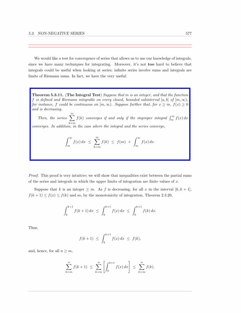
5.3. NON-NEGATIVE SERIES 577
We would like a test for convergence of series that allows us to use our knowledge of integrals,since we have many techniques for integrating. Moreover, it’s not too hard to believe thatintegrals could be useful when looking at series; infinite series involve sums and integrals arelimits of Riemann sums. In fact, we have the very useful:
Theorem 5.3.11. (The Integral Test) Suppose that m is an integer, and that the functionf is defined and Riemann integrable on every closed, bounded subinterval [a, b] of [m,∞),for instance, f could be continuous on [m,∞). Suppose further that, for x ≥ m, f(x) ≥ 0and is decreasing.
Then, the series∞∑k=m
f(k) converges if and only if the improper integral∫∞mf(x) dx
converges. In addition, in the case where the integral and the series converge,
∫ ∞m
f(x) dx ≤∞∑k=m
f(k) ≤ f(m) +∫ ∞m
f(x) dx.
Proof. This proof is very intuitive; we will show that inequalities exist between the partial sumsof the series and integrals in which the upper limits of integration are finite values of x.
Suppose that k is an integer ≥ m. As f is decreasing, for all x in the interval [k, k + 1],f(k + 1) ≤ f(x) ≤ f(k) and so, by the monotonicity of integration, Theorem 2.3.20,
∫ k+1
k
f(k + 1) dx ≤∫ k+1
k
f(x) dx ≤∫ k+1
k
f(k) dx.
Thus,
f(k + 1) ≤∫ k+1
k
f(x) dx ≤ f(k),
and, hence, for all n ≥ m,
n∑k=m
f(k + 1) ≤n∑
k=m
[∫ k+1
k
f(x) dx
]≤
n∑k=m
f(k).
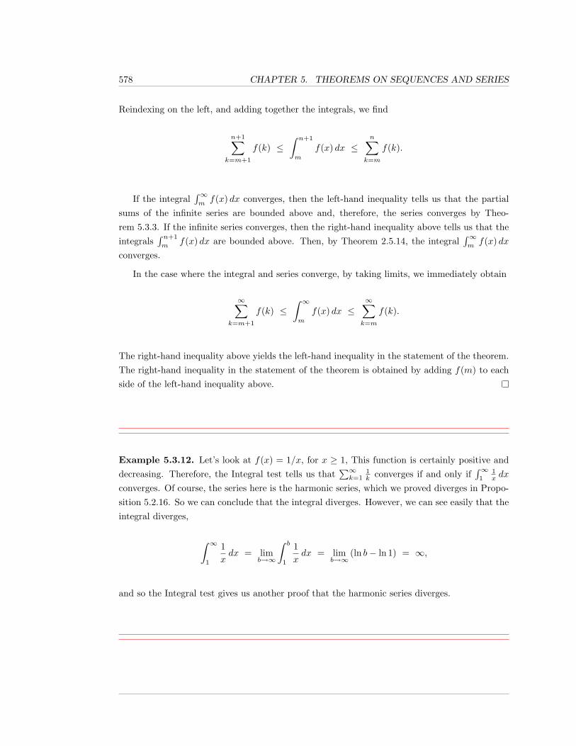
578 CHAPTER 5. THEOREMS ON SEQUENCES AND SERIES
Reindexing on the left, and adding together the integrals, we find
n+1∑k=m+1
f(k) ≤∫ n+1
m
f(x) dx ≤n∑
k=m
f(k).
If the integral∫∞mf(x) dx converges, then the left-hand inequality tells us that the partial
sums of the infinite series are bounded above and, therefore, the series converges by Theo-rem 5.3.3. If the infinite series converges, then the right-hand inequality above tells us that theintegrals
∫ n+1
mf(x) dx are bounded above. Then, by Theorem 2.5.14, the integral
∫∞mf(x) dx
converges.
In the case where the integral and series converge, by taking limits, we immediately obtain
∞∑k=m+1
f(k) ≤∫ ∞m
f(x) dx ≤∞∑k=m
f(k).
The right-hand inequality above yields the left-hand inequality in the statement of the theorem.The right-hand inequality in the statement of the theorem is obtained by adding f(m) to eachside of the left-hand inequality above.
Example 5.3.12. Let’s look at f(x) = 1/x, for x ≥ 1, This function is certainly positive anddecreasing. Therefore, the Integral test tells us that
∑∞k=1
1k converges if and only if
∫∞1
1x dx
converges. Of course, the series here is the harmonic series, which we proved diverges in Propo-sition 5.2.16. So we can conclude that the integral diverges. However, we can see easily that theintegral diverges,
∫ ∞1
1xdx = lim
b→∞
∫ b
1
1xdx = lim
b→∞(ln b− ln 1) = ∞,
and so the Integral test gives us another proof that the harmonic series diverges.
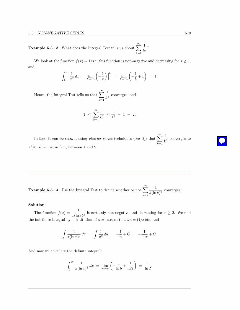
5.3. NON-NEGATIVE SERIES 579
Example 5.3.13. What does the Integral Test tells us about∞∑k=1
1k2
?
We look at the function f(x) = 1/x2; this function is non-negative and decreasing for x ≥ 1,and ∫ ∞
1
1x2
dx = limb→∞
(− 1x
) ∣∣∣b1
= limb→∞
(−1b
+ 1)
= 1.
Hence, the Integral Test tells us that∞∑k=1
1k2
converges, and
1 ≤∞∑k=1
1k2≤ 1
12+ 1 = 2.
In fact, it can be shown, using Fourier series techniques (see [3]) that∞∑k=1
1k2
converges to
π2/6, which is, in fact, between 1 and 2.
Example 5.3.14. Use the Integral Test to decide whether or not∞∑k=2
1k(ln k)2
converges.
Solution:
The function f(x) =1
x(lnx)2is certainly non-negative and decreasing for x ≥ 2. We find
the indefinite integral by substitution of u = lnx, so that du = (1/x)dx, and
∫1
x(lnx)2dx =
∫1u2
du = − 1u
+ C = − 1lnx
+ C.
And now we calculate the definite integral:
∫ ∞2
1x(lnx)2
dx = limb→∞
(− 1
ln b+
1ln 2
)=
1ln 2
.
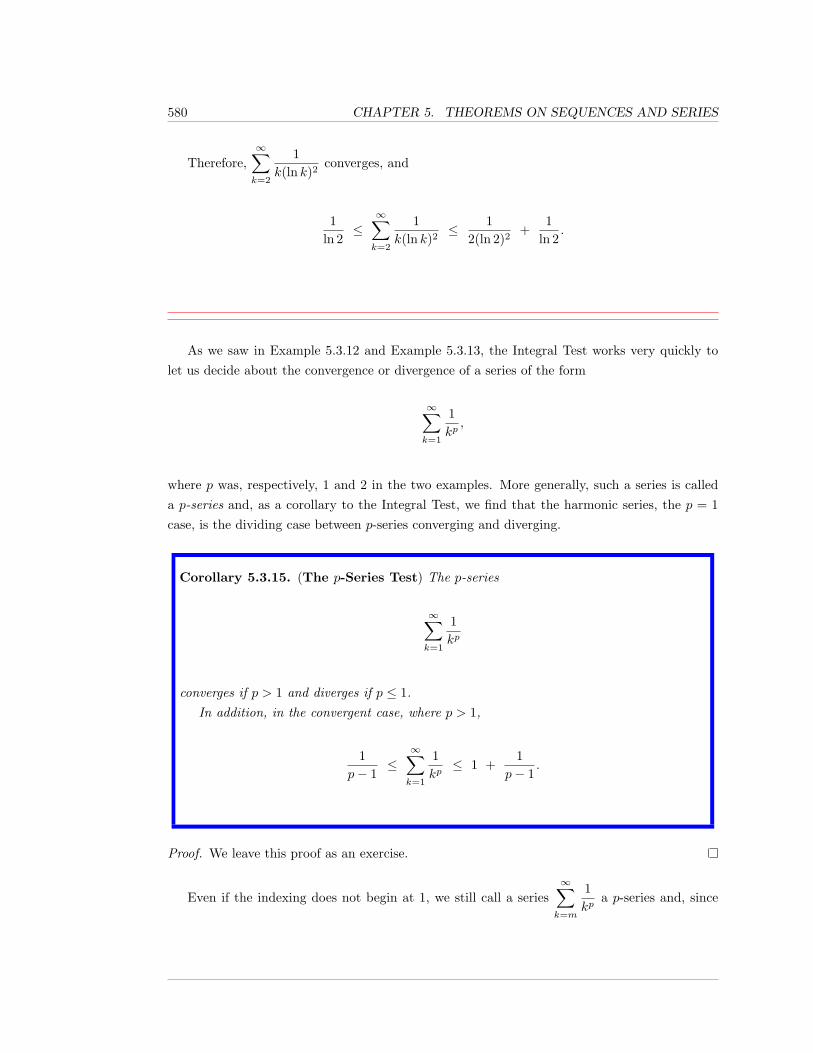
580 CHAPTER 5. THEOREMS ON SEQUENCES AND SERIES
Therefore,∞∑k=2
1k(ln k)2
converges, and
1ln 2
≤∞∑k=2
1k(ln k)2
≤ 12(ln 2)2
+1
ln 2.
As we saw in Example 5.3.12 and Example 5.3.13, the Integral Test works very quickly tolet us decide about the convergence or divergence of a series of the form
∞∑k=1
1kp,
where p was, respectively, 1 and 2 in the two examples. More generally, such a series is calleda p-series and, as a corollary to the Integral Test, we find that the harmonic series, the p = 1case, is the dividing case between p-series converging and diverging.
Corollary 5.3.15. (The p-Series Test) The p-series
∞∑k=1
1kp
converges if p > 1 and diverges if p ≤ 1.In addition, in the convergent case, where p > 1,
1p− 1
≤∞∑k=1
1kp≤ 1 +
1p− 1
.
Proof. We leave this proof as an exercise.
Even if the indexing does not begin at 1, we still call a series∞∑k=m
1kp
a p-series and, since
5.3. NON-NEGATIVE SERIES 581
omitting a finite number of terms does not affect convergence/divergence, such a p-series stillconverges if and only if p > 1.
Example 5.3.16. The p-Series Test tells us immediately that∞∑k=1
1k0.999
diverges, while∞∑k=1
1k1.001
converges to some value v such that 1000 ≤ v ≤ 1001.
It is important not to confuse p-series with geometric series, even though they look verysimilar.
∞∑k=1
12k
is geometric, while∞∑k=1
1k2
is a p-series.
Geometric series have a fixed base and variable exponent, while p-series have a variable baseand a fixed exponent.
Our next convergence test is easy to see. Suppose that we have two sequences of terms,where one is always less than or equal to the other, i.e., for k ≥ m, we have 0 ≤ ak ≤ bk. Then,all of the partial sums satisfy the analogous inequality
n∑k=m
ak ≤n∑
k=m
bk.
Recalling from Theorem 5.3.3 that the only way for a non-negative series to diverge is for itto diverge to ∞, we immediately conclude:
582 CHAPTER 5. THEOREMS ON SEQUENCES AND SERIES
Theorem 5.3.17. (The Comparison Test) Suppose that, for all k ≥ m, we have theinequalities 0 ≤ ak ≤ bk.
1. If∑∞k=m bk converges, then so does
∑∞k=m ak, and
∞∑k=m
ak ≤∞∑k=m
bk.
2. If∑∞k=m ak diverges (necessarily to ∞), then so does
∑∞k=m bk.
Remark 5.3.18. The conclusions of the Comparison Test should not be hard to remember,provided that you keep in mind that the only way for a non-negative series to diverge is for itto diverge to ∞. If you remember this, the Comparison Test basically says that a series beingless than or equal to than something that’s < ∞ implies the series is < ∞, and a series beinggreater than or equal to something that’s ∞ implies that the series is ∞.
If you think about it, it’s also not hard to see what the Comparison Test does not say. Ifthe bigger series diverges, it diverges to ∞, and all you know about the smaller series is that itadds up to something ≤ ∞; but that means that the smaller series could converge to somethingfinite or diverge to ∞, so you conclude nothing. If the smaller series converges, then the biggerseries adds up to something larger, but that something could be finite or ∞, so once again youconclude nothing.
You need for the bigger non-negative series to converge, or the smaller non-negative seriesto diverge in order to conclude anything from the Comparison Test.
Example 5.3.19. Consider the series∞∑k=1
1k2 + 3
and∞∑k=1
1k − 0.5
.
As1
k2 + 3≤ 1k2
, and we know from the p-Series Test that∞∑k=1
1k2
converges, the Comparison
Test tells us that∞∑k=1
1k2 + 3
also converges.
5.3. NON-NEGATIVE SERIES 583
As1
k − 0.5≥ 1
k, for k ≥ 1, and we know that the harmonic series
∞∑k=1
1k
diverges, the
Comparison Test tells us that∞∑k=1
1k − 0.5
also diverges.
Note that the facts that1k2≤ 1k2 − 0.5
and that∞∑k=1
1k2
converges do not allow us to conclude
from the Comparison Test anything about the convergence or divergence of∞∑k=1
1k2 − 0.5
.
What we saw at the end of the example above, that comparing∞∑k=1
1k2
and∞∑k=1
1k2 − 0.5
tells
us nothing about the convergence/divergence of∞∑k=1
1k2 − 0.5
, is somewhat frustrating. Yeah -
it’s true that1k2≤ 1k2 − 0.5
, and yet you may have the feeling that, when k is really big, the
−0.5 just shouldn’t matter – it’s negligible – and the series∞∑k=1
1k2 − 0.5
should do whatever the
series∞∑k=1
1k2
does.
The following theorem says that this line of thinking is valid.
Theorem 5.3.20. (The Limit Comparison Test) Suppose that, for k ≥ m, ak ≥ 0 andbk ≥ 0. Suppose also that
limk→∞
akbk
= L,
where L may be infinity (so, the limit exists as an extended real number).
1. If L 6= 0 and L 6= ∞, then the two series∑∞k=m ak and
∑∞k=m bk do the same thing,
i.e., either both converge or both diverge.
2. If L = 0, and∑∞k=m bk converges, then
∑∞k=m ak converges.
3. If L =∞, and∑∞k=m bk diverges, then
∑∞k=m ak diverges.
Proof. We give the proof in Case 1, and leave the other two cases as an exercise.
So, suppose that
limk→∞
akbk
= L,
584 CHAPTER 5. THEOREMS ON SEQUENCES AND SERIES
where L > 0 is a real number. Note, first, that this means that there has to exist m0 such that,for all k ≥ m0, bk 6= 0, for, otherwise, the fraction doesn’t even exist for arbitrarily large k.
Let ε = L/2 > 0. Then, by definition of the limit of a sequence, there exists an integerN ≥ m0 such that, for all integers n ≥ N ,
∣∣∣∣anbn − L
∣∣∣∣ ≤ ε =L
2.
Thus, for n ≥ N ,
−L2≤ an
bn− L ≤ L
2,
and, hence, (L
2
)bn ≤ an ≤
(3L2
)bn, (5.3)
where we used that bn > 0 for n ≥ N .
Now, suppose that∑∞n=m bn converges. Then, by Proposition 5.2.6,
∑∞n=N bn converges,
and by Theorem 5.2.17,∑∞n=N
(3L2
)bn converges. Hence, using the inequality on the right-
hand side of Formula 5.3 and the Comparison Test, Theorem 5.3.17, we conclude that∑∞n=N an
converges. Applying Proposition 5.2.6 again allows us to conclude that∑∞n=m an converges.
The other conclusion is entirely similar. Suppose that∑∞n=m an converges. Then, by
Proposition 5.2.6,∑∞n=N an converges. Using the inequality on the left-hand side of Formula 5.3
and the Comparison Test, we conclude that∑∞n=N
(L2
)bn converges. By Theorem 5.2.17,∑∞
n=N bn converges. Applying Proposition 5.2.6 again allows us to conclude that∑∞n=m bn
converges.
Example 5.3.21. So, suppose you want to decide whether or not
∞∑k=1
1k2 − 0.5
converges. How do you think about such a problem?
You think the way we discussed before proving the Limit Comparison Test. You think:“when k is big, the 0.5 (added or subtracted) is negligible, and this series should do whatever
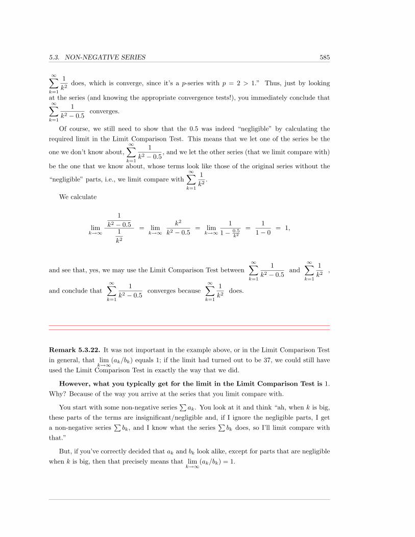
5.3. NON-NEGATIVE SERIES 585
∞∑k=1
1k2
does, which is converge, since it’s a p-series with p = 2 > 1.” Thus, just by looking
at the series (and knowing the appropriate convergence tests!), you immediately conclude that∞∑k=1
1k2 − 0.5
converges.
Of course, we still need to show that the 0.5 was indeed “negligible” by calculating therequired limit in the Limit Comparison Test. This means that we let one of the series be the
one we don’t know about,∞∑k=1
1k2 − 0.5
, and we let the other series (that we limit compare with)
be the one that we know about, whose terms look like those of the original series without the
“negligible” parts, i.e., we limit compare with∞∑k=1
1k2
.
We calculate
limk→∞
1k2 − 0.5
1k2
= limk→∞
k2
k2 − 0.5= lim
k→∞
11− 0.5
k2
=1
1− 0= 1,
and see that, yes, we may use the Limit Comparison Test between∞∑k=1
1k2 − 0.5
and∞∑k=1
1k2
,
and conclude that∞∑k=1
1k2 − 0.5
converges because∞∑k=1
1k2
does.
Remark 5.3.22. It was not important in the example above, or in the Limit Comparison Testin general, that lim
k→∞(ak/bk) equals 1; if the limit had turned out to be 37, we could still have
used the Limit Comparison Test in exactly the way that we did.
However, what you typically get for the limit in the Limit Comparison Test is 1.Why? Because of the way you arrive at the series that you limit compare with.
You start with some non-negative series∑ak. You look at it and think “ah, when k is big,
these parts of the terms are insignificant/negligible and, if I ignore the negligible parts, I geta non-negative series
∑bk, and I know what the series
∑bk does, so I’ll limit compare with
that.”
But, if you’ve correctly decided that ak and bk look alike, except for parts that are negligiblewhen k is big, then that precisely means that lim
k→∞(ak/bk) = 1.
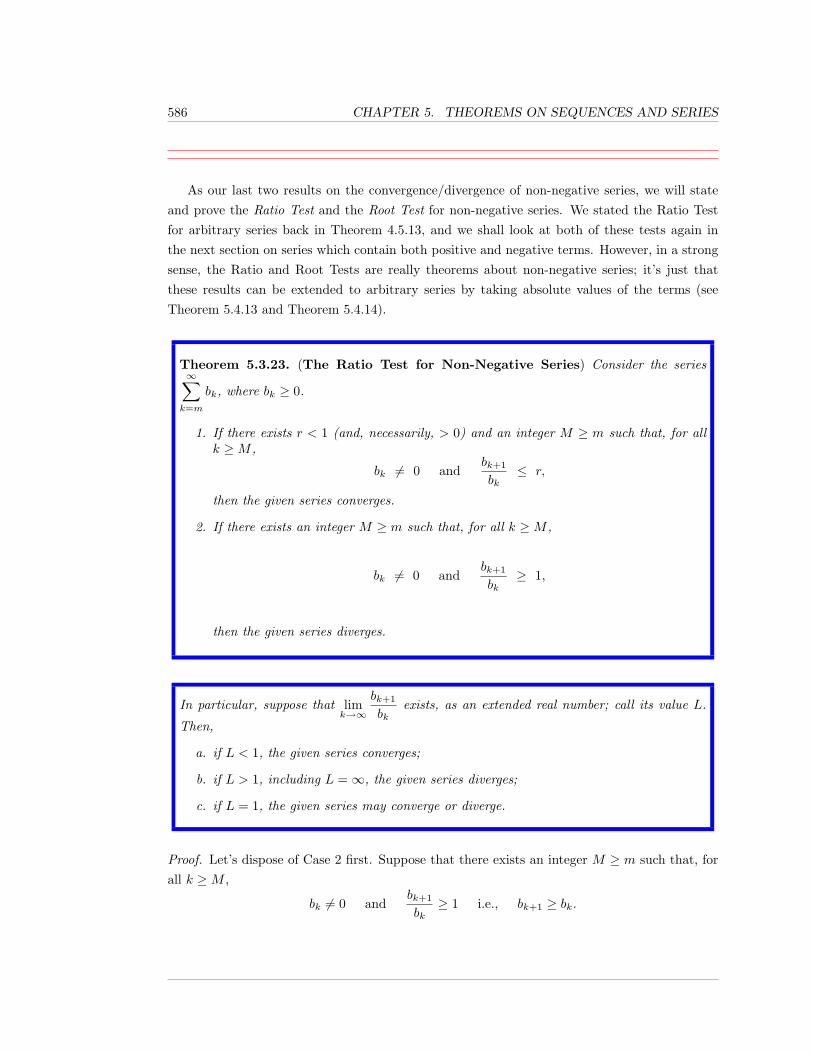
586 CHAPTER 5. THEOREMS ON SEQUENCES AND SERIES
As our last two results on the convergence/divergence of non-negative series, we will stateand prove the Ratio Test and the Root Test for non-negative series. We stated the Ratio Testfor arbitrary series back in Theorem 4.5.13, and we shall look at both of these tests again inthe next section on series which contain both positive and negative terms. However, in a strongsense, the Ratio and Root Tests are really theorems about non-negative series; it’s just thatthese results can be extended to arbitrary series by taking absolute values of the terms (seeTheorem 5.4.13 and Theorem 5.4.14).
Theorem 5.3.23. (The Ratio Test for Non-Negative Series) Consider the series∞∑k=m
bk, where bk ≥ 0.
1. If there exists r < 1 (and, necessarily, > 0) and an integer M ≥ m such that, for allk ≥M ,
bk 6= 0 andbk+1
bk≤ r,
then the given series converges.
2. If there exists an integer M ≥ m such that, for all k ≥M ,
bk 6= 0 andbk+1
bk≥ 1,
then the given series diverges.
In particular, suppose that limk→∞
bk+1
bkexists, as an extended real number; call its value L.
Then,
a. if L < 1, the given series converges;
b. if L > 1, including L =∞, the given series diverges;
c. if L = 1, the given series may converge or diverge.
Proof. Let’s dispose of Case 2 first. Suppose that there exists an integer M ≥ m such that, forall k ≥M ,
bk 6= 0 andbk+1
bk≥ 1 i.e., bk+1 ≥ bk.
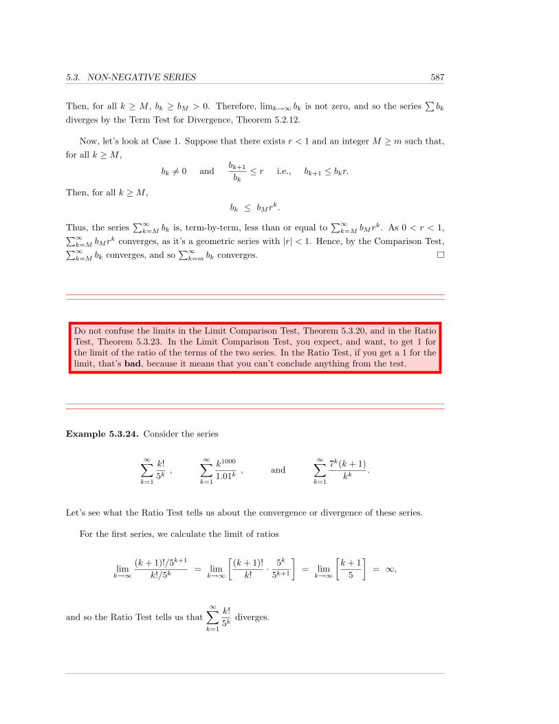
5.3. NON-NEGATIVE SERIES 587
Then, for all k ≥ M , bk ≥ bM > 0. Therefore, limk→∞ bk is not zero, and so the series∑bk
diverges by the Term Test for Divergence, Theorem 5.2.12.
Now, let’s look at Case 1. Suppose that there exists r < 1 and an integer M ≥ m such that,for all k ≥M ,
bk 6= 0 andbk+1
bk≤ r i.e., bk+1 ≤ bkr.
Then, for all k ≥M ,
bk ≤ bMrk.
Thus, the series∑∞k=M bk is, term-by-term, less than or equal to
∑∞k=M bMr
k. As 0 < r < 1,∑∞k=M bMr
k converges, as it’s a geometric series with |r| < 1. Hence, by the Comparison Test,∑∞k=M bk converges, and so
∑∞k=m bk converges.
Do not confuse the limits in the Limit Comparison Test, Theorem 5.3.20, and in the RatioTest, Theorem 5.3.23. In the Limit Comparison Test, you expect, and want, to get 1 forthe limit of the ratio of the terms of the two series. In the Ratio Test, if you get a 1 for thelimit, that’s bad, because it means that you can’t conclude anything from the test.
Example 5.3.24. Consider the series
∞∑k=1
k!5k
,
∞∑k=1
k1000
1.01k, and
∞∑k=1
7k(k + 1)kk
.
Let’s see what the Ratio Test tells us about the convergence or divergence of these series.
For the first series, we calculate the limit of ratios
limk→∞
(k + 1)!/5k+1
k!/5k= lim
k→∞
[(k + 1)!k!
· 5k
5k+1
]= lim
k→∞
[k + 1
5
]= ∞,
and so the Ratio Test tells us that∞∑k=1
k!5k
diverges.
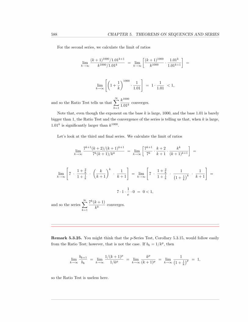
588 CHAPTER 5. THEOREMS ON SEQUENCES AND SERIES
For the second series, we calculate the limit of ratios
limk→∞
(k + 1)1000/1.01k+1
k1000/1.01k= lim
k→∞
[(k + 1)1000
k1000· 1.01k
1.01k+1
]=
limk→∞
[(1 +
1k
)1000
· 11.01
]= 1 · 1
1.01< 1,
and so the Ratio Test tells us that∞∑k=1
k1000
1.01kconverges.
Note that, even though the exponent on the base k is large, 1000, and the base 1.01 is barelybigger than 1, the Ratio Test and the convergence of the series is telling us that, when k is large,1.01k is significantly larger than k1000.
Let’s look at the third and final series. We calculate the limit of ratios
limk→∞
7k+1(k + 2)/(k + 1)k+1
7k(k + 1)/kk= lim
k→∞
[7k+1
7k· k + 2k + 1
· kk
(k + 1)k+1
]=
limk→∞
[7 ·
1 + 2k
1 + 1k
·(
k
k + 1
)k· 1k + 1
]= lim
k→∞
[7 ·
1 + 2k
1 + 1k
· 1(1 + 1
k
)k · 1k + 1
]=
7 · 1 · 1e· 0 = 0 < 1,
and so the series∞∑k=1
7k(k + 1)kk
converges.
Remark 5.3.25. You might think that the p-Series Test, Corollary 5.3.15, would follow easilyfrom the Ratio Test; however, that is not the case. If bk = 1/kp, then
limk→∞
bk+1
bk= lim
k→∞
1/(k + 1)p
1/kp= lim
k→∞
kp
(k + 1)p= lim
k→∞
1(1 + 1
k
)p = 1,
so the Ratio Test is useless here.
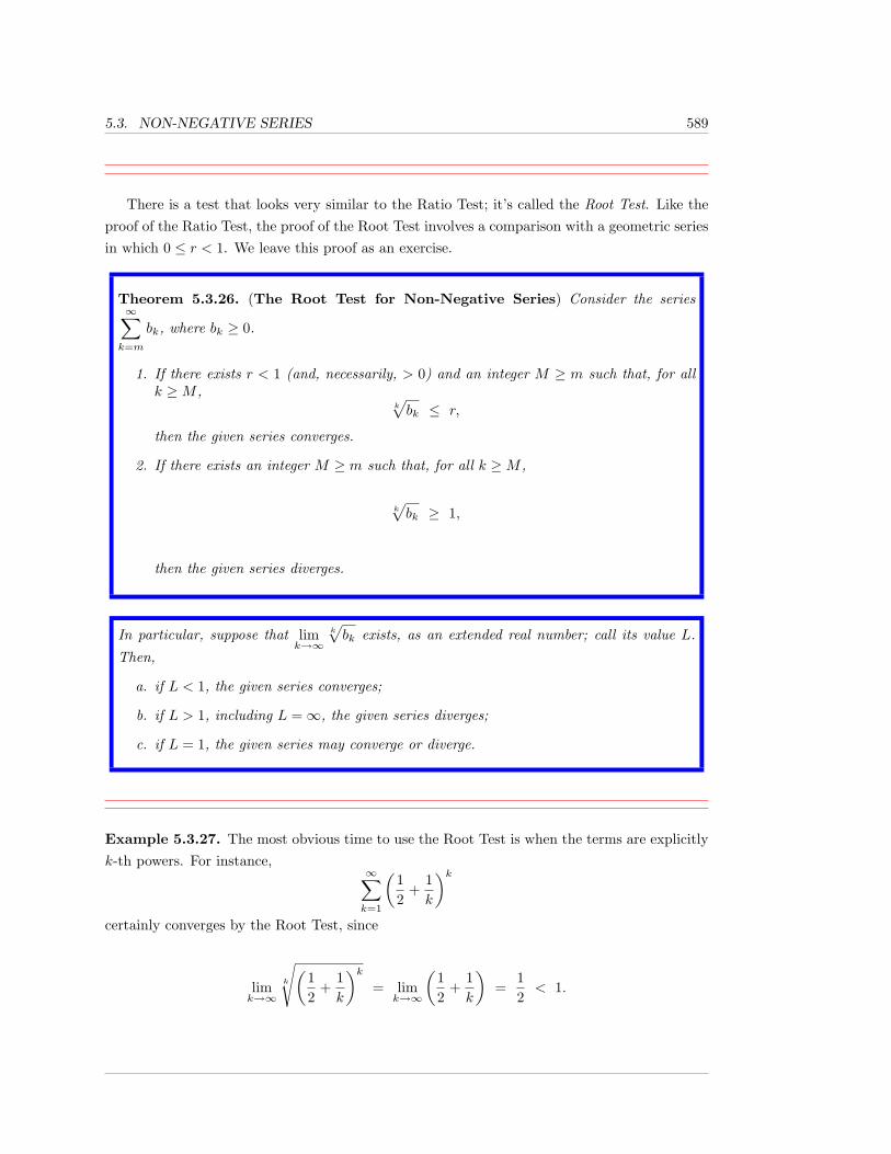
5.3. NON-NEGATIVE SERIES 589
There is a test that looks very similar to the Ratio Test; it’s called the Root Test. Like theproof of the Ratio Test, the proof of the Root Test involves a comparison with a geometric seriesin which 0 ≤ r < 1. We leave this proof as an exercise.
Theorem 5.3.26. (The Root Test for Non-Negative Series) Consider the series∞∑k=m
bk, where bk ≥ 0.
1. If there exists r < 1 (and, necessarily, > 0) and an integer M ≥ m such that, for allk ≥M ,
k√bk ≤ r,
then the given series converges.
2. If there exists an integer M ≥ m such that, for all k ≥M ,
k√bk ≥ 1,
then the given series diverges.
In particular, suppose that limk→∞
k√bk exists, as an extended real number; call its value L.
Then,
a. if L < 1, the given series converges;
b. if L > 1, including L =∞, the given series diverges;
c. if L = 1, the given series may converge or diverge.
Example 5.3.27. The most obvious time to use the Root Test is when the terms are explicitlyk-th powers. For instance,
∞∑k=1
(12
+1k
)kcertainly converges by the Root Test, since
limk→∞
k
√(12
+1k
)k= lim
k→∞
(12
+1k
)=
12< 1.
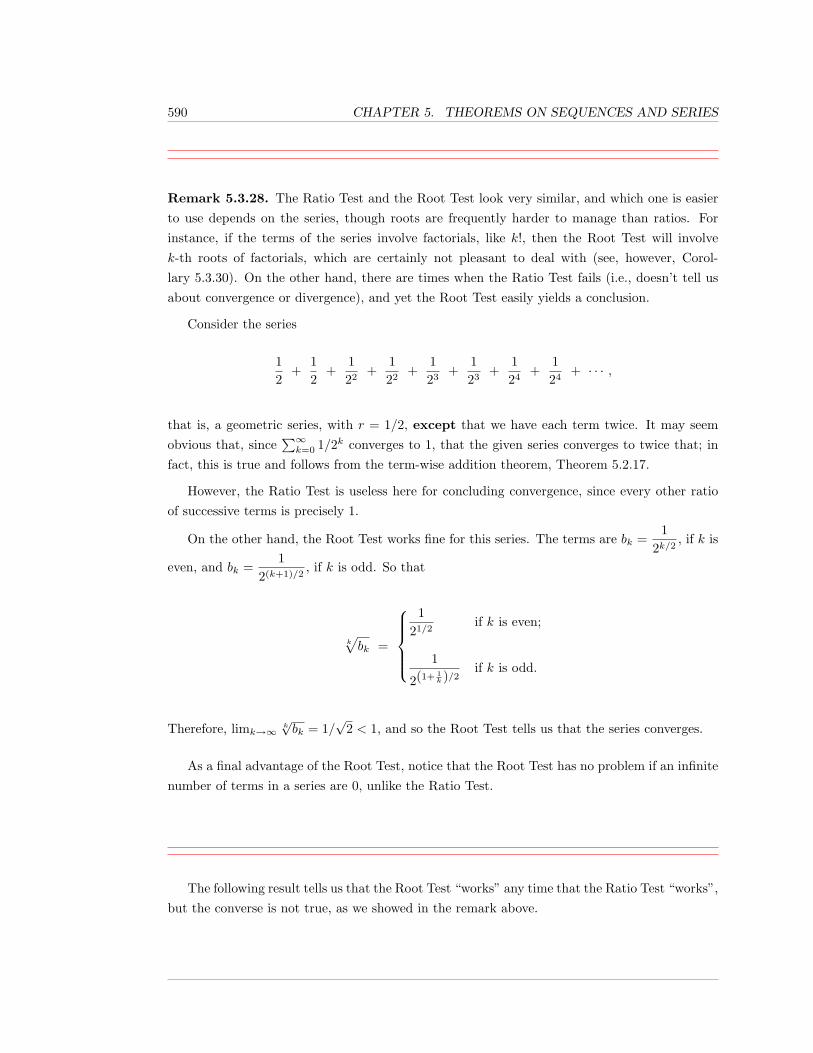
590 CHAPTER 5. THEOREMS ON SEQUENCES AND SERIES
Remark 5.3.28. The Ratio Test and the Root Test look very similar, and which one is easierto use depends on the series, though roots are frequently harder to manage than ratios. Forinstance, if the terms of the series involve factorials, like k!, then the Root Test will involvek-th roots of factorials, which are certainly not pleasant to deal with (see, however, Corol-lary 5.3.30). On the other hand, there are times when the Ratio Test fails (i.e., doesn’t tell usabout convergence or divergence), and yet the Root Test easily yields a conclusion.
Consider the series
12
+12
+122
+122
+123
+123
+124
+124
+ · · · ,
that is, a geometric series, with r = 1/2, except that we have each term twice. It may seemobvious that, since
∑∞k=0 1/2k converges to 1, that the given series converges to twice that; in
fact, this is true and follows from the term-wise addition theorem, Theorem 5.2.17.
However, the Ratio Test is useless here for concluding convergence, since every other ratioof successive terms is precisely 1.
On the other hand, the Root Test works fine for this series. The terms are bk =1
2k/2, if k is
even, and bk =1
2(k+1)/2, if k is odd. So that
k√bk =
1
21/2if k is even;
1
2(1+ 1k )/2
if k is odd.
Therefore, limk→∞k√bk = 1/
√2 < 1, and so the Root Test tells us that the series converges.
As a final advantage of the Root Test, notice that the Root Test has no problem if an infinitenumber of terms in a series are 0, unlike the Ratio Test.
The following result tells us that the Root Test “works” any time that the Ratio Test “works”,but the converse is not true, as we showed in the remark above.
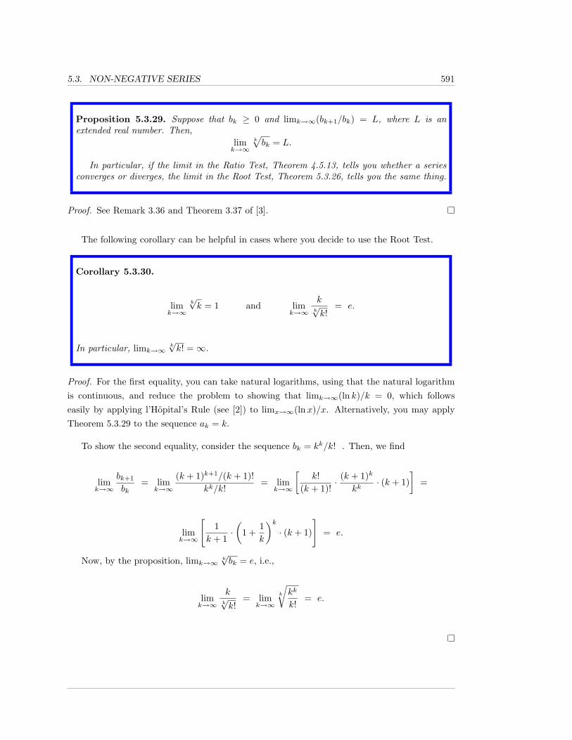
5.3. NON-NEGATIVE SERIES 591
Proposition 5.3.29. Suppose that bk ≥ 0 and limk→∞(bk+1/bk) = L, where L is anextended real number. Then,
limk→∞
k√bk = L.
In particular, if the limit in the Ratio Test, Theorem 4.5.13, tells you whether a seriesconverges or diverges, the limit in the Root Test, Theorem 5.3.26, tells you the same thing.
Proof. See Remark 3.36 and Theorem 3.37 of [3].
The following corollary can be helpful in cases where you decide to use the Root Test.
Corollary 5.3.30.
limk→∞
k√k = 1 and lim
k→∞
kk√k!
= e.
In particular, limk→∞k√k! =∞.
Proof. For the first equality, you can take natural logarithms, using that the natural logarithmis continuous, and reduce the problem to showing that limk→∞(ln k)/k = 0, which followseasily by applying l’Hopital’s Rule (see [2]) to limx→∞(lnx)/x. Alternatively, you may applyTheorem 5.3.29 to the sequence ak = k.
To show the second equality, consider the sequence bk = kk/k! . Then, we find
limk→∞
bk+1
bk= lim
k→∞
(k + 1)k+1/(k + 1)!kk/k!
= limk→∞
[k!
(k + 1)!· (k + 1)k
kk· (k + 1)
]=
limk→∞
[1
k + 1·(
1 +1k
)k· (k + 1)
]= e.
Now, by the proposition, limk→∞k√bk = e, i.e.,
limk→∞
kk√k!
= limk→∞
k
√kk
k!= e.
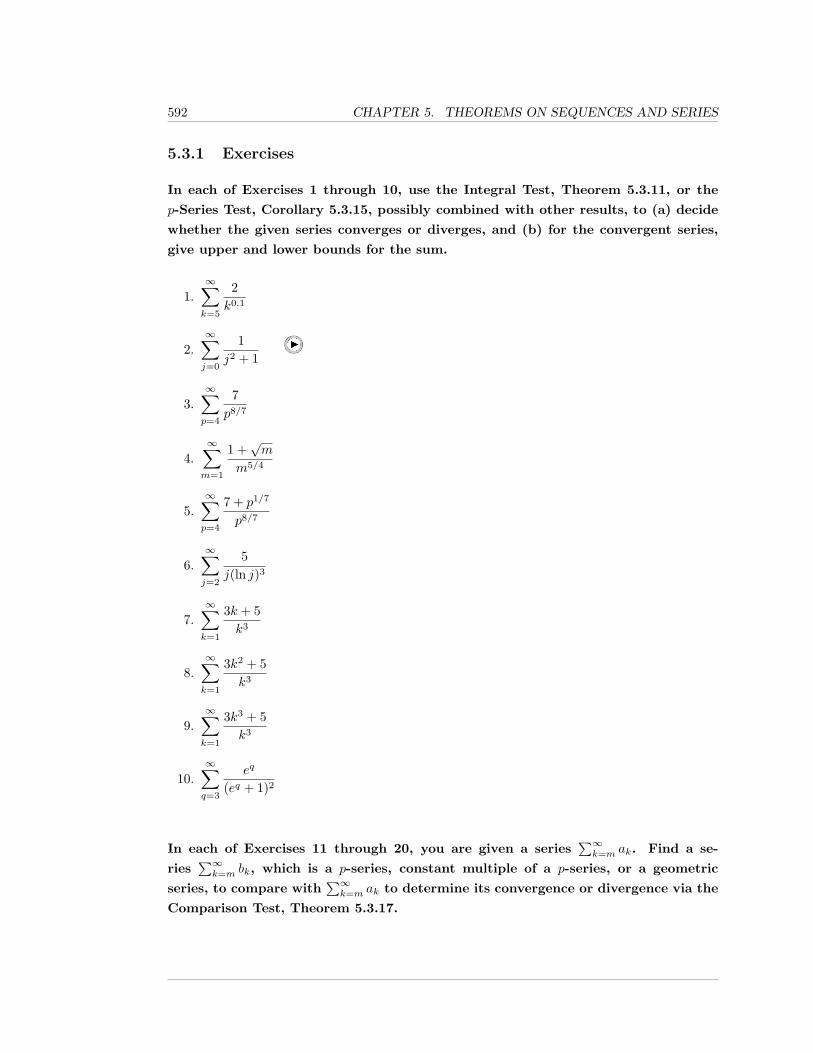
592 CHAPTER 5. THEOREMS ON SEQUENCES AND SERIES
5.3.1 Exercises
In each of Exercises 1 through 10, use the Integral Test, Theorem 5.3.11, or the
p-Series Test, Corollary 5.3.15, possibly combined with other results, to (a) decide
whether the given series converges or diverges, and (b) for the convergent series,
give upper and lower bounds for the sum.
1.∞∑k=5
2k0.1
2.∞∑j=0
1j2 + 1
3.∞∑p=4
7p8/7
4.∞∑m=1
1 +√m
m5/4
5.∞∑p=4
7 + p1/7
p8/7
6.∞∑j=2
5j(ln j)3
7.∞∑k=1
3k + 5k3
8.∞∑k=1
3k2 + 5k3
9.∞∑k=1
3k3 + 5k3
10.∞∑q=3
eq
(eq + 1)2
In each of Exercises 11 through 20, you are given a series∑∞k=m ak. Find a se-
ries∑∞k=m bk, which is a p-series, constant multiple of a p-series, or a geometric
series, to compare with∑∞k=m ak to determine its convergence or divergence via the
Comparison Test, Theorem 5.3.17.
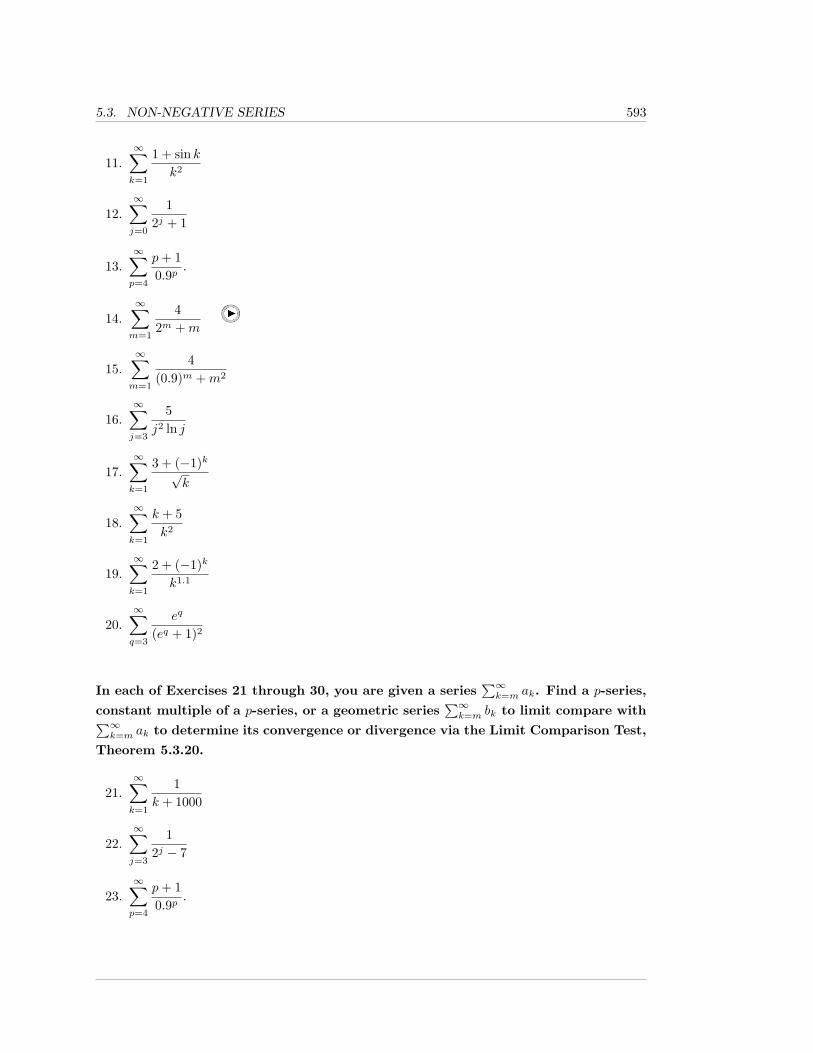
5.3. NON-NEGATIVE SERIES 593
11.∞∑k=1
1 + sin kk2
12.∞∑j=0
12j + 1
13.∞∑p=4
p+ 10.9p
.
14.∞∑m=1
42m +m
15.∞∑m=1
4(0.9)m +m2
16.∞∑j=3
5j2 ln j
17.∞∑k=1
3 + (−1)k√k
18.∞∑k=1
k + 5k2
19.∞∑k=1
2 + (−1)k
k1.1
20.∞∑q=3
eq
(eq + 1)2
In each of Exercises 21 through 30, you are given a series∑∞k=m ak. Find a p-series,
constant multiple of a p-series, or a geometric series∑∞k=m bk to limit compare with∑∞
k=m ak to determine its convergence or divergence via the Limit Comparison Test,
Theorem 5.3.20.
21.∞∑k=1
1k + 1000
22.∞∑j=3
12j − 7
23.∞∑p=4
p+ 10.9p
.
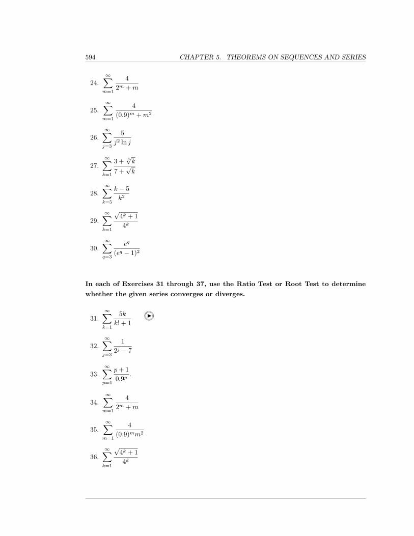
594 CHAPTER 5. THEOREMS ON SEQUENCES AND SERIES
24.∞∑m=1
42m +m
25.∞∑m=1
4(0.9)m +m2
26.∞∑j=3
5j2 ln j
27.∞∑k=1
3 + 3√k
7 +√k
28.∞∑k=5
k − 5k2
29.∞∑k=1
√4k + 14k
30.∞∑q=3
eq
(eq − 1)2
In each of Exercises 31 through 37, use the Ratio Test or Root Test to determine
whether the given series converges or diverges.
31.∞∑k=1
5kk! + 1
32.∞∑j=3
12j − 7
33.∞∑p=4
p+ 10.9p
.
34.∞∑m=1
42m +m
35.∞∑m=1
4(0.9)mm2
36.∞∑k=1
√4k + 14k
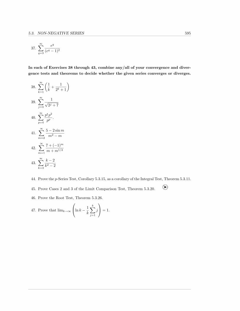
5.3. NON-NEGATIVE SERIES 595
37.∞∑q=3
eq
(eq − 1)2
In each of Exercises 38 through 43, combine any/all of your convergence and diver-
gence tests and theorems to decide whether the given series converges or diverges.
38.∞∑k=1
(1k
+1
2k + 1
)
39.∞∑j=3
1√2j + 7
40.∞∑p=4
p! p2
pp.
41.∞∑m=2
5− 2 sinmm2 −m
42.∞∑m=1
7 + (−1)m
m+m1/2
43.∞∑k=3
k − 2k2 − 2
44. Prove the p-Series Test, Corollary 5.3.15, as a corollary of the Integral Test, Theorem 5.3.11.
45. Prove Cases 2 and 3 of the Limit Comparison Test, Theorem 5.3.20.
46. Prove the Root Test, Theorem 5.3.26.
47. Prove that limk→∞
ln k − 1k
k∑j=1
j
= 1.
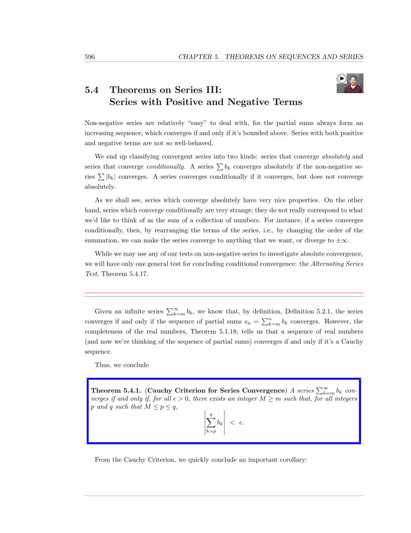
596 CHAPTER 5. THEOREMS ON SEQUENCES AND SERIES
5.4 Theorems on Series III:Series with Positive and Negative Terms
Non-negative series are relatively “easy” to deal with, for the partial sums always form anincreasing sequence, which converges if and only if it’s bounded above. Series with both positiveand negative terms are not so well-behaved.
We end up classifying convergent series into two kinds: series that converge absolutely andseries that converge conditionally. A series
∑bk converges absolutely if the non-negative se-
ries∑|bk| converges. A series converges conditionally if it converges, but does not converge
absolutely.
As we shall see, series which converge absolutely have very nice properties. On the otherhand, series which converge conditionally are very strange; they do not really correspond to whatwe’d like to think of as the sum of a collection of numbers. For instance, if a series convergesconditionally, then, by rearranging the terms of the series, i.e., by changing the order of thesummation, we can make the series converge to anything that we want, or diverge to ±∞.
While we may use any of our tests on non-negative series to investigate absolute convergence,we will have only one general test for concluding conditional convergence: the Alternating SeriesTest, Theorem 5.4.17.
Given an infinite series∑∞k=m bk, we know that, by definition, Definition 5.2.1, the series
converges if and only if the sequence of partial sums sn =∑nk=m bk converges. However, the
completeness of the real numbers, Theorem 5.1.18, tells us that a sequence of real numbers(and now we’re thinking of the sequence of partial sums) converges if and only if it’s a Cauchysequence.
Thus, we conclude
Theorem 5.4.1. (Cauchy Criterion for Series Convergence) A series∑∞k=m bk con-
verges if and only if, for all ε > 0, there exists an integer M ≥ m such that, for all integersp and q such that M ≤ p ≤ q, ∣∣∣∣∣∣
q∑k=p
bk
∣∣∣∣∣∣ < ε.
From the Cauchy Criterion, we quickly conclude an important corollary:
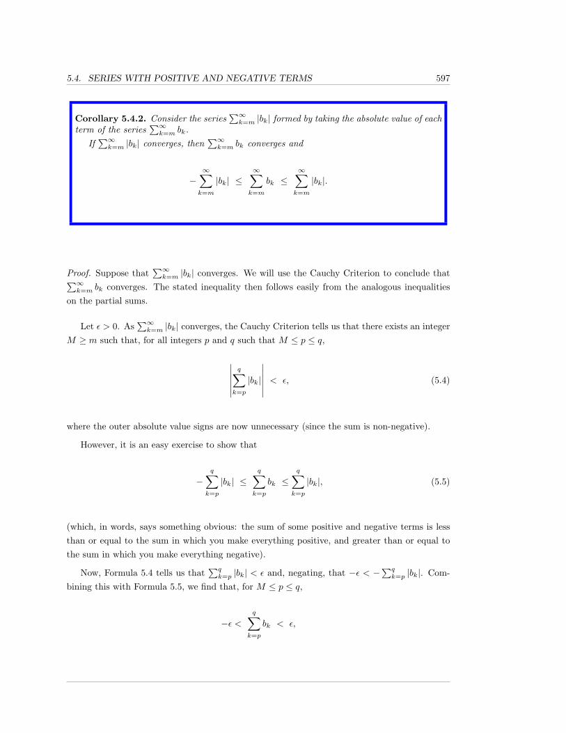
5.4. SERIES WITH POSITIVE AND NEGATIVE TERMS 597
Corollary 5.4.2. Consider the series∑∞k=m |bk| formed by taking the absolute value of each
term of the series∑∞k=m bk.
If∑∞k=m |bk| converges, then
∑∞k=m bk converges and
−∞∑k=m
|bk| ≤∞∑k=m
bk ≤∞∑k=m
|bk|.
Proof. Suppose that∑∞k=m |bk| converges. We will use the Cauchy Criterion to conclude that∑∞
k=m bk converges. The stated inequality then follows easily from the analogous inequalitieson the partial sums.
Let ε > 0. As∑∞k=m |bk| converges, the Cauchy Criterion tells us that there exists an integer
M ≥ m such that, for all integers p and q such that M ≤ p ≤ q,
∣∣∣∣∣∣q∑
k=p
|bk|
∣∣∣∣∣∣ < ε, (5.4)
where the outer absolute value signs are now unnecessary (since the sum is non-negative).
However, it is an easy exercise to show that
−q∑
k=p
|bk| ≤q∑
k=p
bk ≤q∑
k=p
|bk|, (5.5)
(which, in words, says something obvious: the sum of some positive and negative terms is lessthan or equal to the sum in which you make everything positive, and greater than or equal tothe sum in which you make everything negative).
Now, Formula 5.4 tells us that∑qk=p |bk| < ε and, negating, that −ε < −
∑qk=p |bk|. Com-
bining this with Formula 5.5, we find that, for M ≤ p ≤ q,
−ε <q∑
k=p
bk < ε,
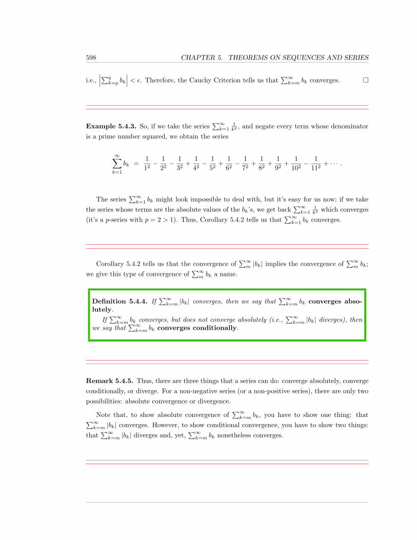
598 CHAPTER 5. THEOREMS ON SEQUENCES AND SERIES
i.e.,∣∣∣∑q
k=p bk
∣∣∣ < ε. Therefore, the Cauchy Criterion tells us that∑∞k=m bk converges.
Example 5.4.3. So, if we take the series∑∞k=1
1k2 , and negate every term whose denominator
is a prime number squared, we obtain the series
∞∑k=1
bk =112− 1
22− 1
32+
142− 1
52+
162− 1
72+
182
+192
+1
102− 1
112+ · · · .
The series∑∞k=1 bk might look impossible to deal with, but it’s easy for us now; if we take
the series whose terms are the absolute values of the bk’s, we get back∑∞k=1
1k2 which converges
(it’s a p-series with p = 2 > 1). Thus, Corollary 5.4.2 tells us that∑∞k=1 bk converges.
Corollary 5.4.2 tells us that the convergence of∑∞m |bk| implies the convergence of
∑∞m bk;
we give this type of convergence of∑∞m bk a name.
Definition 5.4.4. If∑∞k=m |bk| converges, then we say that
∑∞k=m bk converges abso-
lutely.If∑∞k=m bk converges, but does not converge absolutely (i.e.,
∑∞k=m |bk| diverges), then
we say that∑∞k=m bk converges conditionally.
Remark 5.4.5. Thus, there are three things that a series can do: converge absolutely, convergeconditionally, or diverge. For a non-negative series (or a non-positive series), there are only twopossibilities: absolute convergence or divergence.
Note that, to show absolute convergence of∑∞k=m bk, you have to show one thing: that∑∞
k=m |bk| converges. However, to show conditional convergence, you have to show two things:that
∑∞k=m |bk| diverges and, yet,
∑∞k=m bk nonetheless converges.
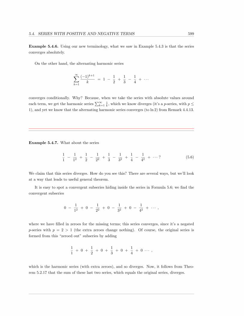
5.4. SERIES WITH POSITIVE AND NEGATIVE TERMS 599
Example 5.4.6. Using our new terminology, what we saw in Example 5.4.3 is that the seriesconverges absolutely.
On the other hand, the alternating harmonic series
∞∑k=1
(−1)k+1
k= 1 − 1
2+
13− 1
4+ · · ·
converges conditionally. Why? Because, when we take the series with absolute values aroundeach term, we get the harmonic series
∑∞k=1
1k , which we know diverges (it’s a p-series, with p ≤
1), and yet we know that the alternating harmonic series converges (to ln 2) from Remark 4.4.13.
Example 5.4.7. What about the series
11− 1
12+
12− 1
22+
13− 1
32+
14− 1
42+ · · · ? (5.6)
We claim that this series diverges. How do you see this? There are several ways, but we’ll lookat a way that leads to useful general theorem.
It is easy to spot a convergent subseries hiding inside the series in Formula 5.6; we find theconvergent subseries
0 − 112
+ 0 − 122
+ 0 − 132
+ 0 − 142
+ · · · ,
where we have filled in zeroes for the missing terms; this series converges, since it’s a negatedp-series with p = 2 > 1 (the extra zeroes change nothing). Of course, the original series isformed from this “zeroed out” subseries by adding
11
+ 0 +12
+ 0 +13
+ 0 +14
+ 0 · · · ,
which is the harmonic series (with extra zeroes), and so diverges. Now, it follows from Theo-rem 5.2.17 that the sum of these last two series, which equals the original series, diverges.
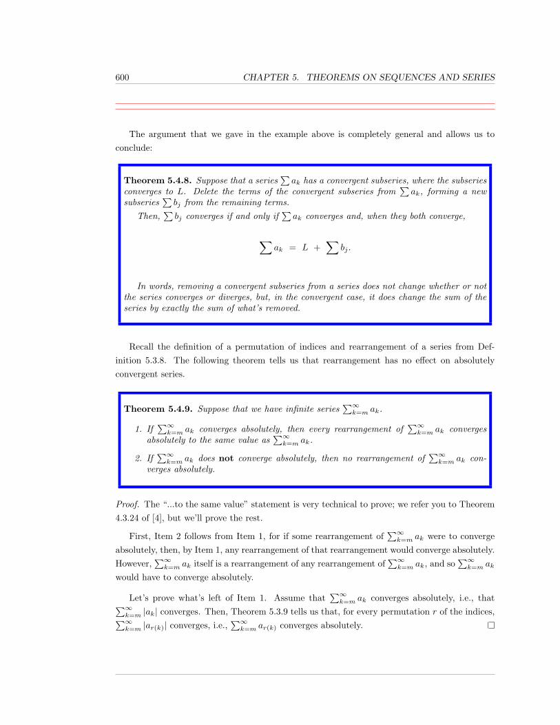
600 CHAPTER 5. THEOREMS ON SEQUENCES AND SERIES
The argument that we gave in the example above is completely general and allows us toconclude:
Theorem 5.4.8. Suppose that a series∑ak has a convergent subseries, where the subseries
converges to L. Delete the terms of the convergent subseries from∑ak, forming a new
subseries∑bj from the remaining terms.
Then,∑bj converges if and only if
∑ak converges and, when they both converge,
∑ak = L +
∑bj .
In words, removing a convergent subseries from a series does not change whether or notthe series converges or diverges, but, in the convergent case, it does change the sum of theseries by exactly the sum of what’s removed.
Recall the definition of a permutation of indices and rearrangement of a series from Def-inition 5.3.8. The following theorem tells us that rearrangement has no effect on absolutelyconvergent series.
Theorem 5.4.9. Suppose that we have infinite series∑∞k=m ak.
1. If∑∞k=m ak converges absolutely, then every rearrangement of
∑∞k=m ak converges
absolutely to the same value as∑∞k=m ak.
2. If∑∞k=m ak does not converge absolutely, then no rearrangement of
∑∞k=m ak con-
verges absolutely.
Proof. The “...to the same value” statement is very technical to prove; we refer you to Theorem4.3.24 of [4], but we’ll prove the rest.
First, Item 2 follows from Item 1, for if some rearrangement of∑∞k=m ak were to converge
absolutely, then, by Item 1, any rearrangement of that rearrangement would converge absolutely.However,
∑∞k=m ak itself is a rearrangement of any rearrangement of
∑∞k=m ak, and so
∑∞k=m ak
would have to converge absolutely.
Let’s prove what’s left of Item 1. Assume that∑∞k=m ak converges absolutely, i.e., that∑∞
k=m |ak| converges. Then, Theorem 5.3.9 tells us that, for every permutation r of the indices,∑∞k=m |ar(k)| converges, i.e.,
∑∞k=m ar(k) converges absolutely.
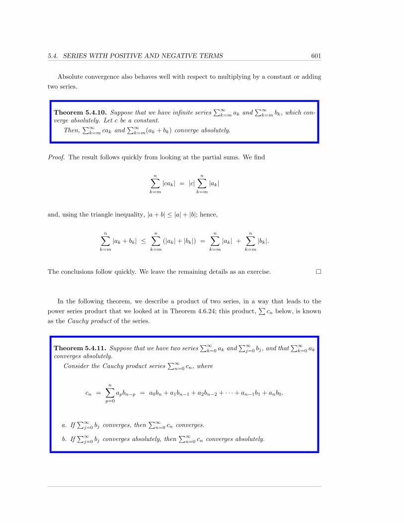
5.4. SERIES WITH POSITIVE AND NEGATIVE TERMS 601
Absolute convergence also behaves well with respect to multiplying by a constant or addingtwo series.
Theorem 5.4.10. Suppose that we have infinite series∑∞k=m ak and
∑∞k=m bk, which con-
verge absolutely. Let c be a constant.Then,
∑∞k=m cak and
∑∞k=m(ak + bk) converge absolutely.
Proof. The result follows quickly from looking at the partial sums. We find
n∑k=m
|cak| = |c|n∑
k=m
|ak|
and, using the triangle inequality, |a+ b| ≤ |a|+ |b|; hence,
n∑k=m
|ak + bk| ≤n∑
k=m
(|ak|+ |bk|) =n∑
k=m
|ak| +n∑
k=m
|bk|.
The conclusions follow quickly. We leave the remaining details as an exercise.
In the following theorem, we describe a product of two series, in a way that leads to thepower series product that we looked at in Theorem 4.6.24; this product,
∑cn below, is known
as the Cauchy product of the series.
Theorem 5.4.11. Suppose that we have two series∑∞k=0 ak and
∑∞j=0 bj, and that
∑∞k=0 ak
converges absolutely.Consider the Cauchy product series
∑∞n=0 cn, where
cn =n∑p=0
apbn−p = a0bn + a1bn−1 + a2bn−2 + · · ·+ an−1b1 + anb0.
a. If∑∞j=0 bj converges, then
∑∞n=0 cn converges.
b. If∑∞j=0 bj converges absolutely, then
∑∞n=0 cn converges absolutely.
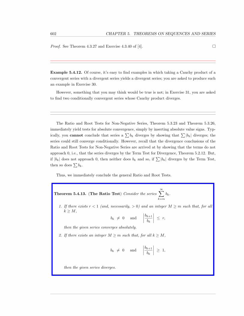
602 CHAPTER 5. THEOREMS ON SEQUENCES AND SERIES
Proof. See Theorem 4.3.27 and Exercise 4.3.40 of [4].
Example 5.4.12. Of course, it’s easy to find examples in which taking a Cauchy product of aconvergent series with a divergent series yields a divergent series; you are asked to produce suchan example in Exercise 30.
However, something that you may think would be true is not; in Exercise 31, you are askedto find two conditionally convergent series whose Cauchy product diverges.
The Ratio and Root Tests for Non-Negative Series, Theorem 5.3.23 and Theorem 5.3.26,immediately yield tests for absolute convergence, simply by inserting absolute value signs. Typ-ically, you cannot conclude that series a
∑bk diverges by showing that
∑|bk| diverges; the
series could still converge conditionally. However, recall that the divergence conclusions of theRatio and Root Tests for Non-Negative Series are arrived at by showing that the terms do notapproach 0, i.e., that the series diverges by the Term Test for Divergence, Theorem 5.2.12. But,if |bk| does not approach 0, then neither does bk and so, if
∑|bk| diverges by the Term Test,
then so does∑bk.
Thus, we immediately conclude the general Ratio and Root Tests.
Theorem 5.4.13. (The Ratio Test) Consider the series∞∑k=m
bk.
1. If there exists r < 1 (and, necessarily, > 0) and an integer M ≥ m such that, for allk ≥M ,
bk 6= 0 and∣∣∣∣bk+1
bk
∣∣∣∣ ≤ r,
then the given series converges absolutely.
2. If there exists an integer M ≥ m such that, for all k ≥M ,
bk 6= 0 and∣∣∣∣bk+1
bk
∣∣∣∣ ≥ 1,
then the given series diverges.
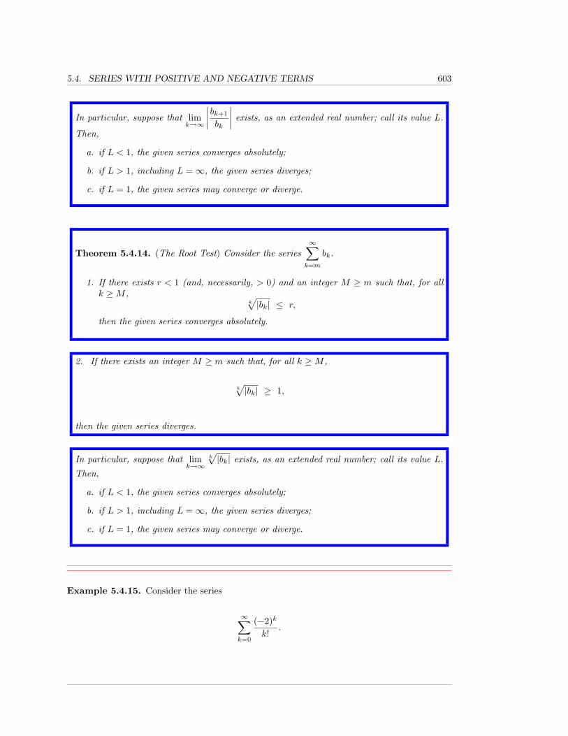
5.4. SERIES WITH POSITIVE AND NEGATIVE TERMS 603
In particular, suppose that limk→∞
∣∣∣∣bk+1
bk
∣∣∣∣ exists, as an extended real number; call its value L.
Then,
a. if L < 1, the given series converges absolutely;
b. if L > 1, including L =∞, the given series diverges;
c. if L = 1, the given series may converge or diverge.
Theorem 5.4.14. (The Root Test) Consider the series∞∑k=m
bk.
1. If there exists r < 1 (and, necessarily, > 0) and an integer M ≥ m such that, for allk ≥M ,
k√|bk| ≤ r,
then the given series converges absolutely.
2. If there exists an integer M ≥ m such that, for all k ≥M ,
k√|bk| ≥ 1,
then the given series diverges.
In particular, suppose that limk→∞
k√|bk| exists, as an extended real number; call its value L.
Then,
a. if L < 1, the given series converges absolutely;
b. if L > 1, including L =∞, the given series diverges;
c. if L = 1, the given series may converge or diverge.
Example 5.4.15. Consider the series
∞∑k=0
(−2)k
k!.
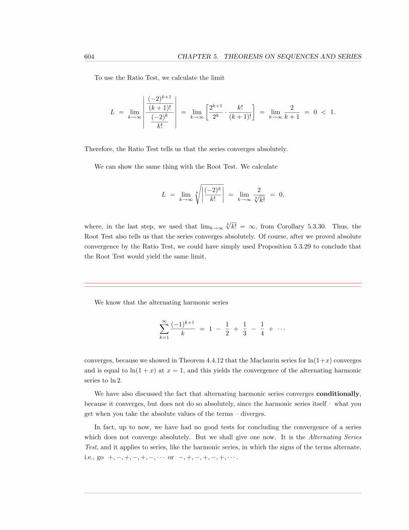
604 CHAPTER 5. THEOREMS ON SEQUENCES AND SERIES
To use the Ratio Test, we calculate the limit
L = limk→∞
∣∣∣∣∣∣∣∣(−2)k+1
(k + 1)!(−2)k
k!
∣∣∣∣∣∣∣∣ = limk→∞
[2k+1
2k· k!
(k + 1)!
]= lim
k→∞
2k + 1
= 0 < 1.
Therefore, the Ratio Test tells us that the series converges absolutely.
We can show the same thing with the Root Test. We calculate
L = limk→∞
k
√∣∣∣∣ (−2)k
k!
∣∣∣∣ = limk→∞
2k√k!
= 0,
where, in the last step, we used that limk→∞k√k! = ∞, from Corollary 5.3.30. Thus, the
Root Test also tells us that the series converges absolutely. Of course, after we proved absoluteconvergence by the Ratio Test, we could have simply used Proposition 5.3.29 to conclude thatthe Root Test would yield the same limit.
We know that the alternating harmonic series
∞∑k=1
(−1)k+1
k= 1 − 1
2+
13− 1
4+ · · ·
converges, because we showed in Theorem 4.4.12 that the Maclaurin series for ln(1+x) convergesand is equal to ln(1 + x) at x = 1, and this yields the convergence of the alternating harmonicseries to ln 2.
We have also discussed the fact that alternating harmonic series converges conditionally,because it converges, but does not do so absolutely, since the harmonic series itself – what youget when you take the absolute values of the terms – diverges.
In fact, up to now, we have had no good tests for concluding the convergence of a serieswhich does not converge absolutely. But we shall give one now. It is the Alternating SeriesTest, and it applies to series, like the harmonic series, in which the signs of the terms alternate,i.e., go +,−,+,−,+,−, · · · or −,+,−,+,−,+, · · · .
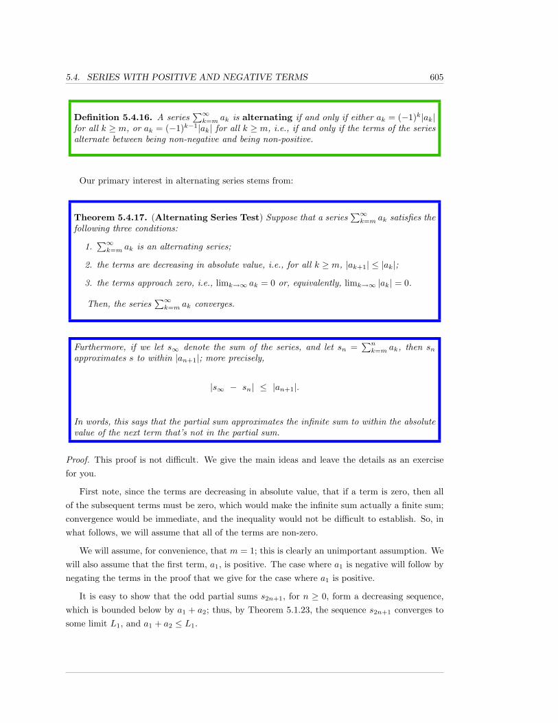
5.4. SERIES WITH POSITIVE AND NEGATIVE TERMS 605
Definition 5.4.16. A series∑∞k=m ak is alternating if and only if either ak = (−1)k|ak|
for all k ≥ m, or ak = (−1)k−1|ak| for all k ≥ m, i.e., if and only if the terms of the seriesalternate between being non-negative and being non-positive.
Our primary interest in alternating series stems from:
Theorem 5.4.17. (Alternating Series Test) Suppose that a series∑∞k=m ak satisfies the
following three conditions:
1.∑∞k=m ak is an alternating series;
2. the terms are decreasing in absolute value, i.e., for all k ≥ m, |ak+1| ≤ |ak|;
3. the terms approach zero, i.e., limk→∞ ak = 0 or, equivalently, limk→∞ |ak| = 0.
Then, the series∑∞k=m ak converges.
Furthermore, if we let s∞ denote the sum of the series, and let sn =∑nk=m ak, then sn
approximates s to within |an+1|; more precisely,
|s∞ − sn| ≤ |an+1|.
In words, this says that the partial sum approximates the infinite sum to within the absolutevalue of the next term that’s not in the partial sum.
Proof. This proof is not difficult. We give the main ideas and leave the details as an exercisefor you.
First note, since the terms are decreasing in absolute value, that if a term is zero, then allof the subsequent terms must be zero, which would make the infinite sum actually a finite sum;convergence would be immediate, and the inequality would not be difficult to establish. So, inwhat follows, we will assume that all of the terms are non-zero.
We will assume, for convenience, that m = 1; this is clearly an unimportant assumption. Wewill also assume that the first term, a1, is positive. The case where a1 is negative will follow bynegating the terms in the proof that we give for the case where a1 is positive.
It is easy to show that the odd partial sums s2n+1, for n ≥ 0, form a decreasing sequence,which is bounded below by a1 + a2; thus, by Theorem 5.1.23, the sequence s2n+1 converges tosome limit L1, and a1 + a2 ≤ L1.
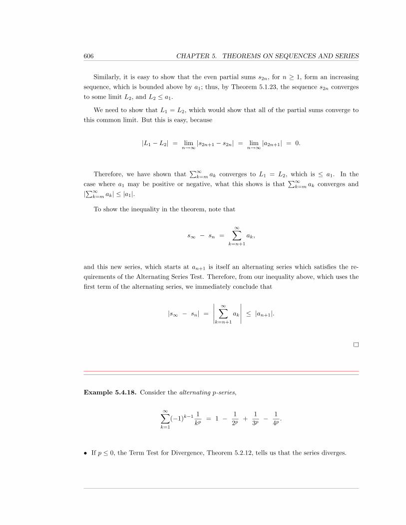
606 CHAPTER 5. THEOREMS ON SEQUENCES AND SERIES
Similarly, it is easy to show that the even partial sums s2n, for n ≥ 1, form an increasingsequence, which is bounded above by a1; thus, by Theorem 5.1.23, the sequence s2n convergesto some limit L2, and L2 ≤ a1.
We need to show that L1 = L2, which would show that all of the partial sums converge tothis common limit. But this is easy, because
|L1 − L2| = limn→∞
|s2n+1 − s2n| = limn→∞
|a2n+1| = 0.
Therefore, we have shown that∑∞k=m ak converges to L1 = L2, which is ≤ a1. In the
case where a1 may be positive or negative, what this shows is that∑∞k=m ak converges and
|∑∞k=m ak| ≤ |a1|.
To show the inequality in the theorem, note that
s∞ − sn =∞∑
k=n+1
ak,
and this new series, which starts at an+1 is itself an alternating series which satisfies the re-quirements of the Alternating Series Test. Therefore, from our inequality above, which uses thefirst term of the alternating series, we immediately conclude that
|s∞ − sn| =
∣∣∣∣∣∞∑
k=n+1
ak
∣∣∣∣∣ ≤ |an+1|.
Example 5.4.18. Consider the alternating p-series,
∞∑k=1
(−1)k−1 1kp
= 1 − 12p
+13p− 1
4p.
• If p ≤ 0, the Term Test for Divergence, Theorem 5.2.12, tells us that the series diverges.
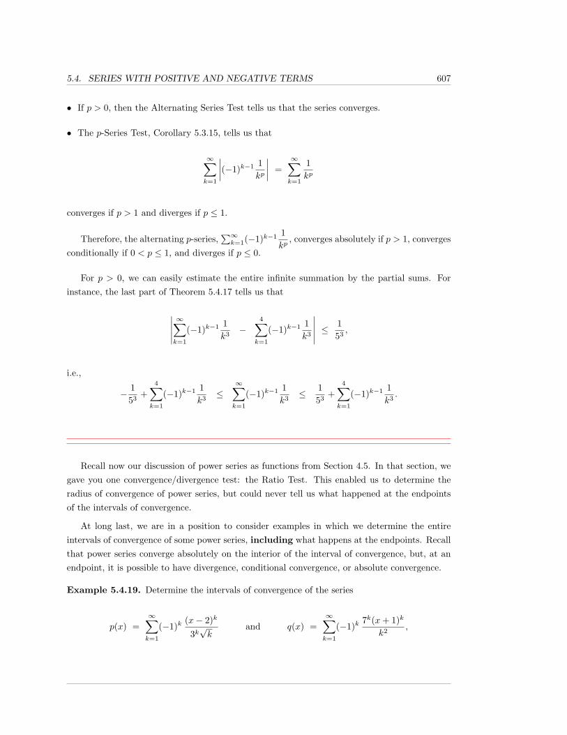
5.4. SERIES WITH POSITIVE AND NEGATIVE TERMS 607
• If p > 0, then the Alternating Series Test tells us that the series converges.
• The p-Series Test, Corollary 5.3.15, tells us that
∞∑k=1
∣∣∣∣(−1)k−1 1kp
∣∣∣∣ =∞∑k=1
1kp
converges if p > 1 and diverges if p ≤ 1.
Therefore, the alternating p-series,∑∞k=1(−1)k−1 1
kp, converges absolutely if p > 1, converges
conditionally if 0 < p ≤ 1, and diverges if p ≤ 0.
For p > 0, we can easily estimate the entire infinite summation by the partial sums. Forinstance, the last part of Theorem 5.4.17 tells us that
∣∣∣∣∣∞∑k=1
(−1)k−1 1k3
−4∑k=1
(−1)k−1 1k3
∣∣∣∣∣ ≤ 153,
i.e.,
− 153
+4∑k=1
(−1)k−1 1k3
≤∞∑k=1
(−1)k−1 1k3
≤ 153
+4∑k=1
(−1)k−1 1k3.
Recall now our discussion of power series as functions from Section 4.5. In that section, wegave you one convergence/divergence test: the Ratio Test. This enabled us to determine theradius of convergence of power series, but could never tell us what happened at the endpointsof the intervals of convergence.
At long last, we are in a position to consider examples in which we determine the entireintervals of convergence of some power series, including what happens at the endpoints. Recallthat power series converge absolutely on the interior of the interval of convergence, but, at anendpoint, it is possible to have divergence, conditional convergence, or absolute convergence.
Example 5.4.19. Determine the intervals of convergence of the series
p(x) =∞∑k=1
(−1)k(x− 2)k
3k√k
and q(x) =∞∑k=1
(−1)k7k(x+ 1)k
k2,
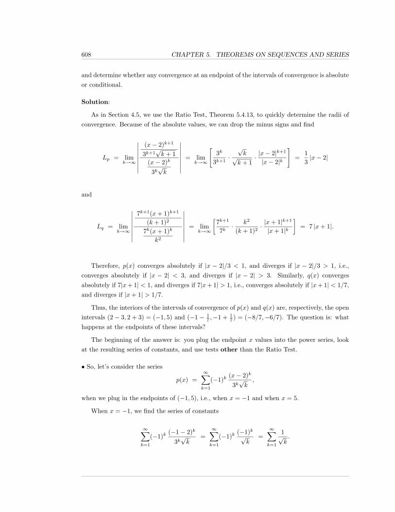
608 CHAPTER 5. THEOREMS ON SEQUENCES AND SERIES
and determine whether any convergence at an endpoint of the intervals of convergence is absoluteor conditional.
Solution:
As in Section 4.5, we use the Ratio Test, Theorem 5.4.13, to quickly determine the radii ofconvergence. Because of the absolute values, we can drop the minus signs and find
Lp = limk→∞
∣∣∣∣∣∣∣∣(x− 2)k+1
3k+1√k + 1
(x− 2)k
3k√k
∣∣∣∣∣∣∣∣ = limk→∞
[3k
3k+1·√k√
k + 1· |x− 2|k+1
|x− 2|k
]=
13|x− 2|
and
Lq = limk→∞
∣∣∣∣∣∣∣∣7k+1(x+ 1)k+1
(k + 1)2
7k(x+ 1)k
k2
∣∣∣∣∣∣∣∣ = limk→∞
[7k+1
7k· k2
(k + 1)2· |x+ 1|k+1
|x+ 1|k
]= 7 |x+ 1|.
Therefore, p(x) converges absolutely if |x − 2|/3 < 1, and diverges if |x − 2|/3 > 1, i.e.,converges absolutely if |x − 2| < 3, and diverges if |x − 2| > 3. Similarly, q(x) convergesabsolutely if 7|x+ 1| < 1, and diverges if 7|x+ 1| > 1, i.e., converges absolutely if |x+ 1| < 1/7,and diverges if |x+ 1| > 1/7.
Thus, the interiors of the intervals of convergence of p(x) and q(x) are, respectively, the openintervals (2− 3, 2 + 3) = (−1, 5) and (−1− 1
7 ,−1 + 17 ) = (−8/7,−6/7). The question is: what
happens at the endpoints of these intervals?
The beginning of the answer is: you plug the endpoint x values into the power series, lookat the resulting series of constants, and use tests other than the Ratio Test.
• So, let’s consider the series
p(x) =∞∑k=1
(−1)k(x− 2)k
3k√k,
when we plug in the endpoints of (−1, 5), i.e., when x = −1 and when x = 5.
When x = −1, we find the series of constants
∞∑k=1
(−1)k(−1− 2)k
3k√k
=∞∑k=1
(−1)k(−1)k√
k=
∞∑k=1
1√k.
5.4. SERIES WITH POSITIVE AND NEGATIVE TERMS 609
This is a p-series, with p = 1/2, and so it diverges by the p-series Test, Corollary 5.3.15.
When x = 5, we find the series of constants
∞∑k=1
(−1)k3k
3k√k
=∞∑k=1
(−1)k1√k.
This is an alternating series, which converges by Theorem 5.4.17; note that the series does notconverge absolutely, as taking the absolute values of the terms would yield the previous divergentp-series with p = 1/2.
Hence, we find that the interval of convergence of p(x) is the interval (−1, 5], and the con-vergence is conditional at x = 5.
• Now, let’s consider the series
q(x) =∞∑k=1
(−1)k7k(x+ 1)k
k2,
when we plug in the endpoints of (−8/7,−6/7), i.e., when x = −8/7 and when x = −6/7.
You can quickly see that, when we plug in these endpoints, we get∑∞k=1
1k2 and
∑∞k=1
(−1)k
k2 ,respectively. These both converge absolutely, by the p-series Test, Corollary 5.3.15, with p = 2.
Hence, we find that the interval of convergence is the closed interval [−8/7,−6/7], and thatq(x) converges absolutely everywhere in the interval.
As the final result of this section, we wish to state, and give an idea of the proof of, a resultthat tells us that the summation in a conditionally convergent series does not correspond towhat we normally think of as adding together a collection of numbers; the theorem tells us thatthe order in which we add the terms in a conditionally convergent series can have a dramatic
effect on the summation. This is not the case for absolutely convergent series, as we saw inTheorem 5.4.9.
610 CHAPTER 5. THEOREMS ON SEQUENCES AND SERIES
Theorem 5.4.20. Suppose that we have infinite series∑∞k=m ak, which converges condi-
tionally. Let L be any extended real number.Then, there exists a rearrangement of the series
∑∞k=m ar(k) such that
∞∑k=m
ar(k) = L.
In words, a conditionally convergent series can be rearranged to converge to anythingwhatsoever, or diverge to ±∞.
Proof. The details of the proof can be found in Theorem 4.3.26 of [4], but will try here toindicate how such a thing is possible.
Let P denote the sum of the positive terms of∑∞k=m ak, taken in order, and let N denote
the sum of the negative terms of∑∞k=m ak, taken in order.
P and N are defined by non-negative and non-positive subseries, respectively, and we mayassume that we have inserted zeroes for each “missing” term of each subseries. This enables usto write P =
∑∞k=m bk and N =
∑∞k=m ck, where bk ≥ 0, ck ≤ 0, and ak = bk + ck.
We claim that P = ∞ and N = −∞. Why is this true? As∑bk and
∑ck are non-
negative and non-positive, respectively, the only choice other than equaling ±∞ is that theseries converge. But, if either one of these series converges, then, since
∑∞k=m ak converges,
Theorem 5.4.8 tells us that the other series must also converge. However, as∑bk and
∑ck are
non-negative and non-positive, the only way for them to converge is absolutely, which wouldimply, by Theorem 5.4.10, that their sum
∑ak converges absolutely. This would contradict
that∑ak converges conditionally.
Therefore, the sum of the positive terms of∑ak is ∞, and the sum of the negative terms is
−∞.
What does this have to do with anything? Well...intuitively, things are fairly easy now. Ifyou want to produce a rearrangement of
∑ak that diverges to ∞, then you simply put lots of
(sizable) positive terms first, then a negative term, then lots of positive terms, then a negativeterm; the point being that by adding together lots of positive terms early, you can overwhelmthe sporadic negative terms. You have to have every negative term in the series somewhere,but they can come after big chunks of positive terms that add up to arbitrarily large positivenumbers.
Similarly, to produce a rearrangement that diverges to −∞ just take lots of (sizable) negativeterms early, then a positive term, and keep going.
5.4. SERIES WITH POSITIVE AND NEGATIVE TERMS 611
Once you believe that there are rearrangements that yield ∞ and −∞, it’s easy to believe,if you were very careful with picking your rearrangement, that you could make it add up toanything between −∞ and ∞, i.e., make the rearrangement add up to any real number what-soever.
5.4.1 Exercises
In each of Exercises 1 through 15, determine whether the given series converges
absolutely, converges conditionally, or diverges. We omit the starting and final
values for the index on the summation; assume the starting index is big enough so
that all of the terms are defined and the final value is ∞.
1.∑ sin k
k2
2.∑ −2 + sin k
k
3.∑ −2 + sin k
k3
4.∑
(−1)k1√k + 4
5.∑
(−1)k√
1 +4k
6.∑(
5k3/2
+ (−1)k−1 13k + 4
)
7.∑(
(−1)k−1 5k3/2
+1
3k + 4
)
8.∑ (−1)k
3(k!) + 4
9.∑ (−1)k√
3(k!) + 4
10.∑ (−1)k
k ln k
11.∑(
3 +(−1)k
k ln k
)
612 CHAPTER 5. THEOREMS ON SEQUENCES AND SERIES
12.∑ cos(kπ/2)
k5 ln k
13.∑ cos(kπ/2)√
k
14.∑
(−1)k−1
√k3 + 1√k5 + 1
15.∑
(−1)k−1
√k3 + 1√k6 + 1
In each of Exercises 16 through 19, find the first 5 terms of the Cauchy product
of the two given series; see Theorem 5.4.11. Also prove that each Cauchy product
converges.
16.∞∑k=0
(−1)k1
(k + 1)2and
∞∑j=0
(−1)j1
j + 1
17.∞∑k=0
1(k + 1)2
and∞∑j=0
(−1)j1
j + 1
18.∞∑k=0
1k!
and∞∑j=0
(−1)j1√j + 1
19.∞∑k=0
(−1)k1k!
and∞∑j=0
1j!
In each of Exercises 20 through 23, show that the alternating series converges, and
give a partial sum which estimates the entire sum of the infinite series to within
0.01.
20.∞∑k=1
(−1)k−1 1k
21.∞∑k=1
(−1)k−1 1√k
22.∞∑k=1
(−1)k−1 1k2
23.∞∑k=1
(−1)k−1 1√k2 + 1
5.4. SERIES WITH POSITIVE AND NEGATIVE TERMS 613
24. If∑an converges absolutely and
∑bn converges absolutely, what can you say about∑
(an + bn)?
25. If∑an converges absolutely and
∑bn converges conditionally, what can you say about∑
(an + bn)?
26. If∑an converges conditionally and
∑bn converges conditionally, what can you say about∑
(an + bn)?
27. If∑an converges absolutely and
∑bn diverges, what can you say about
∑(an + bn)?
28. If∑an converges conditionally and
∑bn diverges, what can you say about
∑(an + bn)?
29. Complete the proof of Theorem 5.4.10.
30. Give an example of an absolutely convergent series and a divergent series such that theCauchy product (see Theorem 5.4.11) of the two series diverges.
31. Find two conditionally convergent series whose Cauchy product diverges.
32. Fill in the details of the proof of the Alternating Series Test, Theorem 5.4.17.
33. Write a brief essay, in which you discuss the ways in which conditionally convergent seriesdo not behave like “normal” sums of numbers.
34. Suppose you have a power series p(x) =∑∞k=0 ck(x − a)k, with radius of convergence R.
Prove that, if p(x) converges absolutely at one end of the interval of convergence, thenit converges absolutely at the other end. Is the same statement true if “absolutely” isreplaced both times with “conditionally”?
In each of Exercises 35 through 42, you are given a power series from the Exercises
in Section 4.5, for which you may have already found the radius of convergence.
Finish finding the precise interval of convergence by determining what happens at
the endpoints of the interval, i.e., if the power series has radius of convergence R,
where 0 < R ≤ ∞, and is centered at a, determine whether the series converges
absolutely, converges conditionally, or diverges at x = a−R and x = a+R.
35.
p(x) =∞∑k=1
5k(x− 1)k
k2= 5(x− 1) +
52
22(x− 1)2 +
53
32(x− 1)3 +
54
42(x− 1)4 + · · · .
614 CHAPTER 5. THEOREMS ON SEQUENCES AND SERIES
36.
p(x) =∞∑k=1
√k (x+ 3)k =
(x+ 3
)+√
2(x+ 3
)2 +√
3(x+ 3
)3 +√
4(x+ 3
)4 + · · · .
37.
p(x) =∞∑k=0
(−1)kxk
k3 + 2=
12− x
13 + 2+
x2
23 + 2− x3
33 + 2+
x4
43 + 2− · · · .
38. p(x) =∞∑k=0
(x− 4)k
7k+1.
39. p(x) =∞∑k=1
(x− 4)k
7k+1k.
40. p(x) =∞∑k=1
(−1)k+1 (x+ 7)k
kk.
41. p(x) =∞∑k=1
(−1)k+1 k!(x+ 7)k
kk.
42. p(x) =∞∑k=1
(−1)k+1 xk
3√k.
Appendix A
An Introduction to Vectors andMotion
A brief introduction to vectors in 2 and 3 dimensions
A vector is frequently described in physics and engineering classes as something which hasa magnitude and a direction. Typical physical vector quantities in the plane are things such as“move north 3 miles”, “travel west at 5 meters per second”, and “a force of 10 pounds pushingsouth”.
A vector in the real line, R, the xy-plane, R2, or xyz-space, R3, is usually represented byan arrow, which points in the direction of the vector and has length equal to the magnitude ofthe vector (even if vector itself does not have length units). However, the arrow representing agiven vector has no fixed starting and ending point; parallel arrows which have the same lengthand which have their tails and heads at corresponding ends (i.e., point in the same direction)represent the same vector.
A vector in the real line is simply a real number r. The magnitude of r is the absolute value|r|. There are two possible “directions” for a vector in the real line; if r > 0, then r has thepositive direction and, if r < 0, then r has the negative direction. The zero vector r = 0 is saidto have every direction (in this case, both directions); this is convenient in statements of someresults, and makes sense, in that, moving 0 feet in the positive direction is the same as moving0 feet in the negative direction.
We shall now discuss vectors in R2. The analogous statements and definitions for vectors inR3 should be clear, and we will explicitly state many of them after our discussion about vectorsin the plane.
We denote the arrow from the point (a, b) to the point (c, d) by−−−−−−−→(a, b)(c, d). Two arrows
615
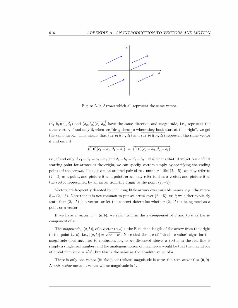
616 APPENDIX A. AN INTRODUCTION TO VECTORS AND MOTION
Figure A.1: Arrows which all represent the same vector.
−−−−−−−−−−→(a1, b1)(c1, d1) and
−−−−−−−−−−→(a2, b2)(c2, d2) have the same direction and magnitude, i.e., represent the
same vector, if and only if, when we “drag them to where they both start at the origin”, we getthe same arrow. This means that
−−−−−−−−−−→(a1, b1)(c1, d1) and
−−−−−−−−−−→(a2, b2)(c2, d2) represent the same vector
if and only if−−−−−−−−−−−−−−−−→(0, 0)(c1 − a1, d1 − b1) =
−−−−−−−−−−−−−−−−→(0, 0)(c2 − a2, d2 − b2),
i.e., if and only if c1− a1 = c2− a2 and d1− b1 = d2− b2. This means that, if we set our defaultstarting point for arrows as the origin, we can specify vectors simply by specifying the endingpoints of the arrows. Thus, given an ordered pair of real numbers, like (2,−5), we may refer to(2,−5) as a point, and picture it as a point, or we may refer to it as a vector, and picture it asthe vector represented by an arrow from the origin to the point (2,−5).
Vectors are frequently denoted by including little arrows over variable names, e.g., the vector~v = (2,−5). Note that it is not common to put an arrow over (2,−5) itself; we either explicitlystate that (2,−5) is a vector, or let the context determine whether (2,−5) is being used as apoint or a vector.
If we have a vector ~v = (a, b), we refer to a as the x-component of ~v and to b as the y-component of ~v.
The magnitude, |(a, b)|, of a vector (a, b) is the Euclidean length of the arrow from the originto the point (a, b), i.e., |(a, b)| =
√a2 + b2. Note that the use of “absolute value” signs for the
magnitude does not lead to confusion, for, as we discussed above, a vector in the real line issimply a single real number, and the analogous notion of magnitude would be that the magnitudeof a real number a is
√a2, but this is the same as the absolute value of a.
There is only one vector (in the plane) whose magnitude is zero: the zero vector ~0 = (0, 0).A unit vector means a vector whose magnitude is 1.
617
We define two other operations on vectors, vector addition and scalar multiplication. Thesum of two vectors (a, b) and (c, d) is defined by adding the corresponding components:
(a, b) + (c, d) = (a+ c, b+ d).
The fact that we are adding the ordered pairs means that we are using them as vectors, notpoints. The scalar multiplication r(a, b) of the vector (a, b) by a real number (a scalar) r isdefined by
r(a, b) = (ra, rb).
If r 6= 0, then(
1r
)~v is frequently written as
~v
r.
From the definition of scalar multiplication, it follows quickly that |r(a, b)| = |r| · |(a, b)|.Multiplying by a positive scalar leaves the direction of the vector unchanged, but “scales” themagnitude because, if r > 0, then |r(a, b)| = |r| · |(a, b)| = r|(a, b)|. Multiplying by a negativescalar produces a vector which points in the opposite direction from the original vector, but themagnitude is scaled by the absolute value of the scalar; thus, −2~v has twice the magnitude of~v, but points in the opposite direction.
The negation, −~v, of a vector ~v is equal to −1~v. Subtraction of vectors ~v = (a, b) and~w = (c, d) is defined component-wise, so that ~v − ~w = (a− c, b− d). This is written in terms ofvector addition and scalar multiplication as
~v − ~w = ~v + (−1~w).
Note that the distance between two points (a, b) and (c, d) is simply the magnitude of the vector(a, b)− (c, d) (or (c, d)− (a, b)).
If ~v 6= ~0, then there is a unique unit vector in the direction of ~v, namely,~v
|~v|. In fact,
since most directions in the plane, using your intuitive notion of “direction”, do not have some
predetermined name, the direction of a non-zero vector ~v is defined to be the unit vector~v
|~v|.
As in the case of “vectors” in the real line, we say that the zero vector ~0 has every direction.
The dot product of two vectors ~v = (a, b) and ~w = (c, d) is defined by
(a, b) · (c, d) = ac+ bd,
i.e., you multiply corresponding components and add. Note that the dot product of two vectors
618 APPENDIX A. AN INTRODUCTION TO VECTORS AND MOTION
is not a vector; it is a real number (a scalar). The dot product has a number of nice properties:for all vectors ~u, ~v, and ~w, and scalars a and b,
1. (commutativity) ~v · ~w = ~w · ~v;
2. (distributivity/linearity) ~u · (a~v + b~w) = a(~u · ~v) + b(~u · ~w); and
3. ~v · ~v = |~v|2.
However, the reason that the dot product is of great interest is because it has the followinggeometric interpretation
~v · ~w = |~v| |~w| cos θ,
where θ is the angle between the vectors ~v and ~w. In particular this means that ~v and ~w areperpendicular if and only if ~v · ~w = 0; note that our convention that the zero vector has every
direction makes this statement true even if ~v or ~w is the zero vector.
Vectors in R3 work just like vectors in R2, except that you now have three components,instead of two. We also frequently refer to R2 as being contained in R3 by thinking of the pointor vector (a, b, 0) as being the same as the point or vector (a, b), i.e., it is standard to think ofthe xy-plane as being the same as the plane where z = 0 inside xyz-space.
Given an ordered triple of real numbers, like (2,−5, 3), we may refer to (2,−5, 3) as a point,and picture it as a point, or we may refer to it as a vector, and picture it as the vector representedby an arrow from the origin to the point (2,−5, 3).
If we have a vector ~v = (a, b, c), we refer to a as the x-component of ~v, to b as the y-componentof ~v, and to c as the z-component.
The magnitude, |(a, b, c)|, of a vector (a, b, c) is the Euclidean length of the arrow from theorigin to the point (a, b, c), i.e., |(a, b)| =
√a2 + b2 + c2.
There is only one vector in R3 whose magnitude is zero: the zero vector ~0 = (0, 0, 0). A unitvector means a vector whose magnitude is 1.
We define vector addition and scalar multiplication as you would expect: the sum of twovectors (a, b, c) and (d, e, f) is defined by adding the corresponding components:
(a, b, c) + (d, e, f) = (a+ d, b+ e, c+ f).
The scalar multiplication r(a, b, c) of the vector (a, b, c) by a real number (a scalar) r is definedby
r(a, b, c) = (ra, rb, rc).
619
If ~v 6= ~0, then there is a unique unit vector in the direction of ~v, namely,~v
|~v|. As in the case
of “vectors” in R and R2, we say that the zero vector ~0 has every direction.
The dot product of two vectors ~v = (a, b, c) and ~w = (d, e, f) is defined by
(a, b, c) · (d, e, f) = ad+ be+ cf,
i.e., you multiply corresponding components and add. The dot product in R3 has the same niceproperties as it did in R2: for all vectors ~u, ~v, and ~w, and scalars a and b,
1. (commutativity) ~v · ~w = ~w · ~v;
2. (distributivity/linearity) ~u · (a~v + b~w) = a(~u · ~v) + b(~u · ~w); and
3. ~v · ~v = |~v|2.
In addition, it is still true in R3 that
~v · ~w = |~v| |~w| cos θ,
where θ is the angle between the vectors ~v and ~w.
Vector-valued functions
Suppose we have a function ~p(t) = (x(t), y(t)) or ~p(t) = (x(t), y(t), z(t)), whose domain is asubset of the real numbers and whose codomain is a subset of either R2 or R3; this is a vector-valued function. The functions x(t), y(t), and z(t) are the component functions of ~p(t). Sucha function ~p(t) is continuous if and only if each of its component functions is continuous; sucha function is differentiable if and only if each of its component functions is differentiable and,
when this is the case, the derivatived~p
dt= ~p ′(t) is defined by
~p ′(t) = limh→0
~p(t+ h)− ~p(t)h
= (x′(t), y′(t)) or (x′(t), y′(t), z′(t)).
Differentiation of vector-valued functions is linear: if ~p(t) and ~q(t) are differentiable vector-valued functions, both in Rn for the same n, and a and b are constants (scalars), then a ~p(t)+b ~q(t)is differentiable and (
a ~p(t) + b ~q(t))′ = a ~p ′(t) + b ~q ′(t).
620 APPENDIX A. AN INTRODUCTION TO VECTORS AND MOTION
More surprising is that there is a product rule for the dot product: if ~p(t) and ~q(t) are dif-ferentiable vector-valued functions, both in Rn for the same n, then ~p(t) · ~q(t) is differentiableand
(~p(t) · ~q(t)
)′ = ~p(t) · ~q ′(t) + ~p ′(t) · ~q(t).
An immediate consequence of this is that, if ~p(t) is differentiable and always has magnitude 1(i.e., is always a unit vector), then 1 = ~p(t) · ~p(t) for all t; therefore, differentiating with respectto t and applying the Product Rule, we find
0 = 2 ~p(t) · ~p ′(t),
so that ~p(t) is always perpendicular to ~p ′(t).
Motion in the plane and in space
We will now discuss motion in the plane and in space. Throughout our discussion, we shalluse notation for the case of motion in R3. The case of motion in R2 is analogous; simply ignorethe z-component in what we write, or take the z-component to be zero.
Suppose that an object is moving in R3. Then, at each time t, the object has an x-coordinate,x(t), a y-coordinate, y(t), and a z-coordinate, z(t). The functions x(t), y(t), and z(t) are saidto describe a parameterized curve in space. The position vector (or, simply position), ~p(t), ofthe object, at time t, is simply the vector (x(t), y(t), z(t)). In place of x(t), y(t), and z(t), it iscommon to write px(t), py(t), and pz(t), respectively, for the x-, y-, and z-components of ~p(t).
If the position function ~p(t) is differentiable, the velocity vector (or, simply, velocity), ~v(t),of the object, at time t, is the derivative of the position vector, i.e.,
~v(t) =d
dt~p(t) = ~p ′(t).
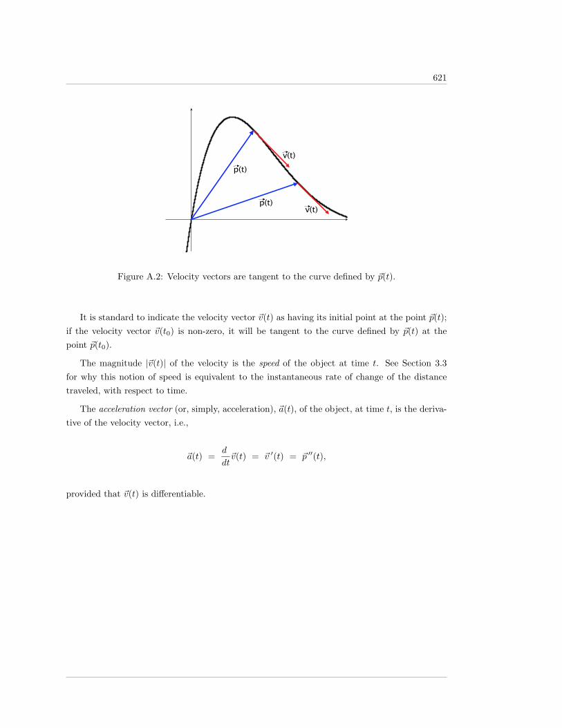
621
p(t)
p(t)
v(t)
v(t)
Figure A.2: Velocity vectors are tangent to the curve defined by ~p(t).
It is standard to indicate the velocity vector ~v(t) as having its initial point at the point ~p(t);if the velocity vector ~v(t0) is non-zero, it will be tangent to the curve defined by ~p(t) at thepoint ~p(t0).
The magnitude |~v(t)| of the velocity is the speed of the object at time t. See Section 3.3for why this notion of speed is equivalent to the instantaneous rate of change of the distancetraveled, with respect to time.
The acceleration vector (or, simply, acceleration), ~a(t), of the object, at time t, is the deriva-tive of the velocity vector, i.e.,
~a(t) =d
dt~v(t) = ~v ′(t) = ~p ′′(t),
provided that ~v(t) is differentiable.

622 APPENDIX A. AN INTRODUCTION TO VECTORS AND MOTION
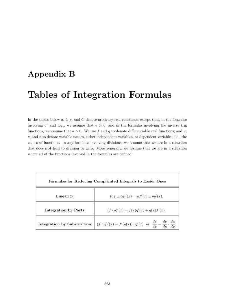
Appendix B
Tables of Integration Formulas
In the tables below a, b, p, and C denote arbitrary real constants, except that, in the formulasinvolving bx and logb, we assume that b > 0, and in the formulas involving the inverse trigfunctions, we assume that a > 0. We use f and g to denote differentiable real functions, and u,v, and x to denote variable names, either independent variables, or dependent variables, i.e., thevalues of functions. In any formulas involving divisions, we assume that we are in a situationthat does not lead to division by zero. More generally, we assume that we are in a situationwhere all of the functions involved in the formulas are defined.
Formulas for Reducing Complicated Integrals to Easier Ones
Linearity: (af ± bg)′(x) = af ′(x)± bg′(x).
Integration by Parts: (f · g)′(x) = f(x)g′(x) + g(x)f ′(x).
Integration by Substitution: (f ◦ g)′(x) = f ′(g(x)) · g′(x) ordv
dx=dv
du· dudx
.
623
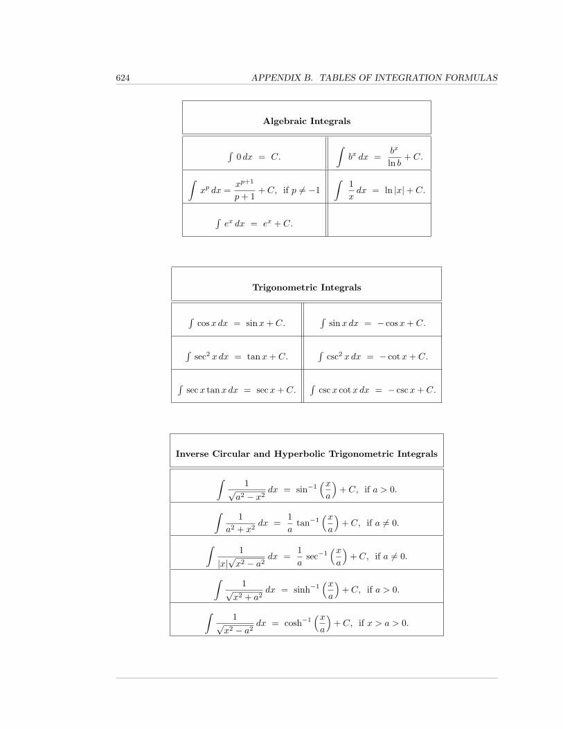
624 APPENDIX B. TABLES OF INTEGRATION FORMULAS
Algebraic Integrals
∫0 dx = C.
∫bx dx =
bx
ln b+ C.
∫xp dx =
xp+1
p+ 1+ C, if p 6= −1
∫1xdx = ln |x|+ C.
∫ex dx = ex + C.
Trigonometric Integrals
∫cosx dx = sinx+ C.
∫sinx dx = − cosx+ C.
∫sec2 x dx = tanx+ C.
∫csc2 x dx = − cotx+ C.
∫secx tanx dx = secx+ C.
∫cscx cotx dx = − cscx+ C.
Inverse Circular and Hyperbolic Trigonometric Integrals
∫1√
a2 − x2dx = sin−1
(xa
)+ C, if a > 0.
∫1
a2 + x2dx =
1a
tan−1(xa
)+ C, if a 6= 0.
∫1
|x|√x2 − a2
dx =1a
sec−1(xa
)+ C, if a 6= 0.
∫1√
x2 + a2dx = sinh−1
(xa
)+ C, if a > 0.
∫1√
x2 − a2dx = cosh−1
(xa
)+ C, if x > a > 0.
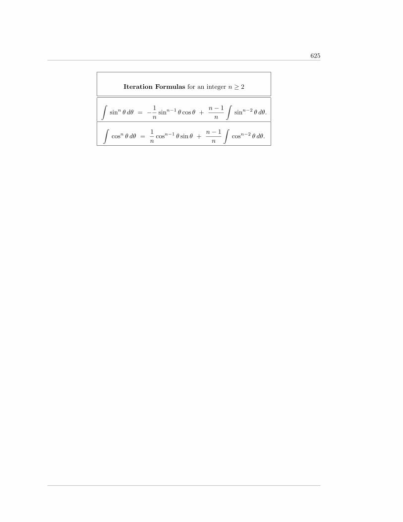
625
Iteration Formulas for an integer n ≥ 2
∫sinn θ dθ = − 1
nsinn−1 θ cos θ +
n− 1n
∫sinn−2 θ dθ.
∫cosn θ dθ =
1n
cosn−1 θ sin θ +n− 1n
∫cosn−2 θ dθ.

626 APPENDIX B. TABLES OF INTEGRATION FORMULAS
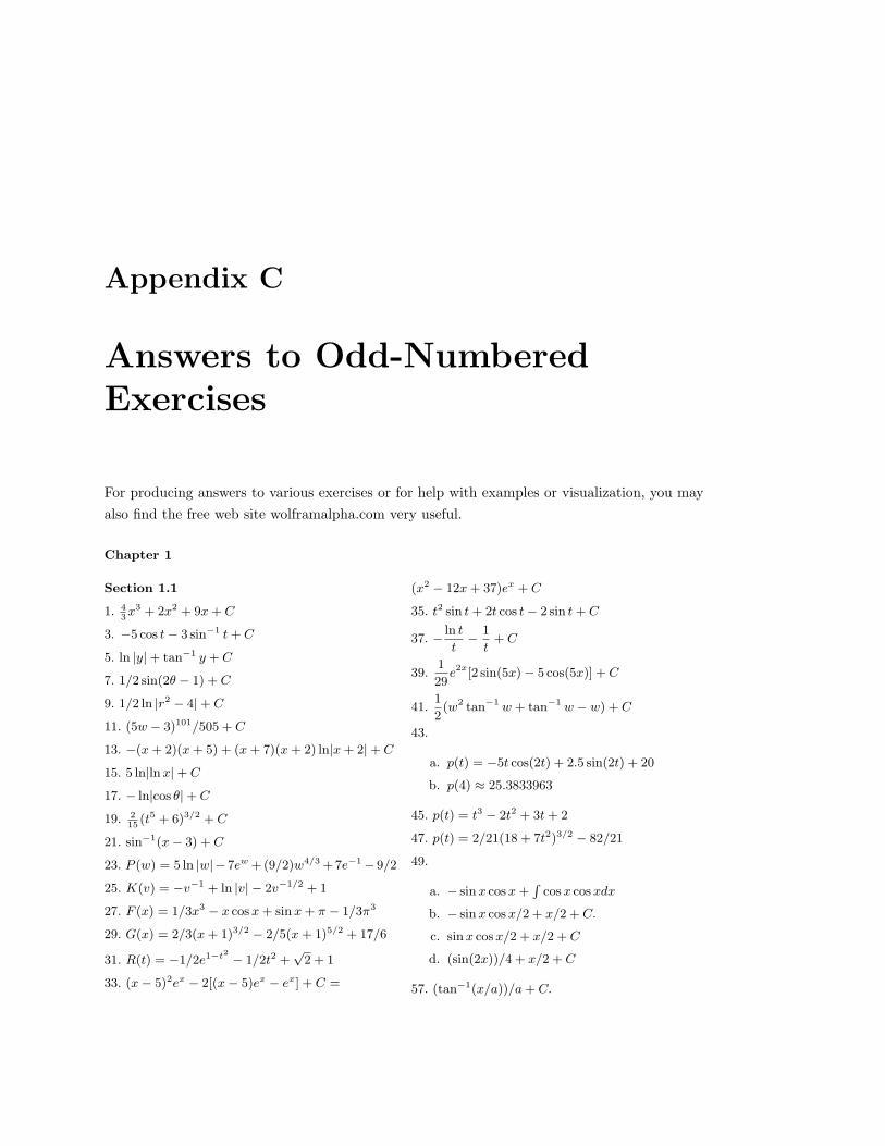
Appendix C
Answers to Odd-NumberedExercises
For producing answers to various exercises or for help with examples or visualization, you mayalso find the free web site wolframalpha.com very useful.
Chapter 1
Section 1.1
1. 43x3 + 2x2 + 9x+ C
3. −5 cos t− 3 sin−1 t+ C
5. ln |y|+ tan−1 y + C
7. 1/2 sin(2θ − 1) + C
9. 1/2 ln |r2 − 4|+ C
11. (5w − 3)101/505 + C
13. −(x+ 2)(x+ 5) + (x+ 7)(x+ 2) ln|x+ 2|+ C
15. 5 ln|lnx|+ C
17. − ln|cos θ|+ C
19. 215
(t5 + 6)3/2 + C
21. sin−1(x− 3) + C
23. P (w) = 5 ln |w|− 7ew + (9/2)w4/3 + 7e−1− 9/2
25. K(v) = −v−1 + ln |v| − 2v−1/2 + 1
27. F (x) = 1/3x3 − x cosx+ sinx+ π − 1/3π3
29. G(x) = 2/3(x+ 1)3/2 − 2/5(x+ 1)5/2 + 17/6
31. R(t) = −1/2e1−t2− 1/2t2 +
√2 + 1
33. (x− 5)2ex − 2[(x− 5)ex − ex] + C =
(x2 − 12x+ 37)ex + C
35. t2 sin t+ 2t cos t− 2 sin t+ C
37. − ln t
t− 1
t+ C
39.1
29e2x[2 sin(5x)− 5 cos(5x)] + C
41.1
2(w2 tan−1 w + tan−1 w − w) + C
43.
a. p(t) = −5t cos(2t) + 2.5 sin(2t) + 20
b. p(4) ≈ 25.3833963
45. p(t) = t3 − 2t2 + 3t+ 2
47. p(t) = 2/21(18 + 7t2)3/2 − 82/21
49.
a. − sinx cosx+R
cosx cosxdx
b. − sinx cosx/2 + x/2 + C.
c. sinx cosx/2 + x/2 + C
d. (sin(2x))/4 + x/2 + C
57. (tan−1(x/a))/a+ C.
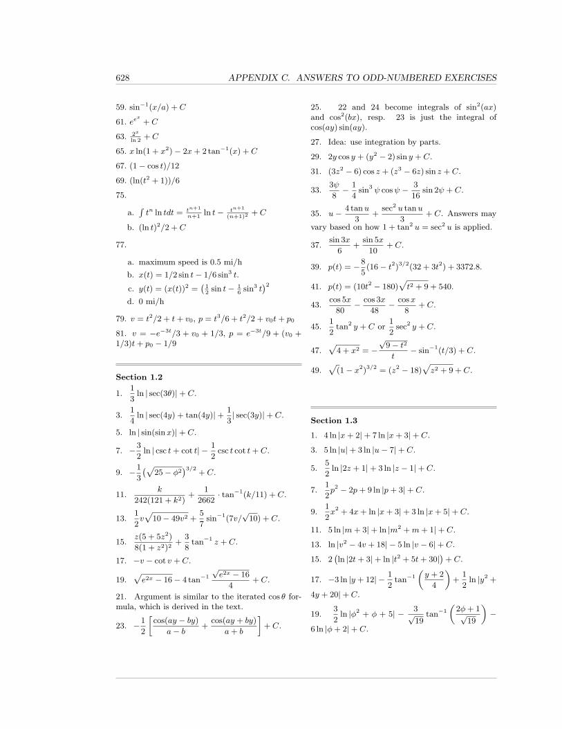
628 APPENDIX C. ANSWERS TO ODD-NUMBERED EXERCISES
59. sin−1(x/a) + C
61. eex
+ C
63. 2x
ln 2+ C
65. x ln(1 + x2)− 2x+ 2 tan−1(x) + C
67. (1− cos t)/12
69. (ln(t2 + 1))/6
75.
a.Rtn ln tdt = tn+1
n+1ln t− tn+1
(n+1)2+ C
b. (ln t)2/2 + C
77.
a. maximum speed is 0.5 mi/h
b. x(t) = 1/2 sin t− 1/6 sin3 t.
c. y(t) = (x(t))2 =`
12
sin t− 16
sin3 t´2
d. 0 mi/h
79. v = t2/2 + t+ v0, p = t3/6 + t2/2 + v0t+ p0
81. v = −e−3t/3 + v0 + 1/3, p = e−3t/9 + (v0 +1/3)t+ p0 − 1/9
Section 1.2
1.1
3ln | sec(3θ)|+ C.
3.1
4ln | sec(4y) + tan(4y)|+ 1
3| sec(3y)|+ C.
5. ln | sin(sinx)|+ C.
7. −3
2ln | csc t+ cot t| − 1
2csc t cot t+ C.
9. −1
3
`p25− φ2
´3/2+ C.
11.k
242(121 + k2)+
1
2662· tan−1(k/11) + C.
13.1
2vp
10− 49v2 +5
7sin−1(7v/
√10) + C.
15.z(5 + 5z2)
8(1 + z2)2+
3
8tan−1 z + C.
17. −v − cot v + C.
19.pe2x − 16− 4 tan−1
√e2x − 16
4+ C.
21. Argument is similar to the iterated cos θ for-mula, which is derived in the text.
23. −1
2
»cos(ay − by)
a− b +cos(ay + by)
a+ b
–+ C.
25. 22 and 24 become integrals of sin2(ax)and cos2(bx), resp. 23 is just the integral ofcos(ay) sin(ay).
27. Idea: use integration by parts.
29. 2y cos y + (y2 − 2) sin y + C.
31. (3z2 − 6) cos z + (z3 − 6z) sin z + C.
33.3ψ
8− 1
4sin3 ψ cosψ − 3
16sin 2ψ + C.
35. u− 4 tanu
3+
sec2 u tanu
3+ C. Answers may
vary based on how 1 + tan2 u = sec2 u is applied.
37.sin 3x
6+
sin 5x
10+ C.
39. p(t) = −8
5(16− t2)3/2(32 + 3t2) + 3372.8.
41. p(t) = (10t2 − 180)pt2 + 9 + 540.
43.cos 5x
80− cos 3x
48− cosx
8+ C.
45.1
2tan2 y + C or
1
2sec2 y + C.
47.p
4 + x2 = −√
9− t2t
− sin−1(t/3) + C.
49.p
(1− x2)3/2 = (z2 − 18)pz2 + 9 + C.
Section 1.3
1. 4 ln |x+ 2|+ 7 ln |x+ 3|+ C.
3. 5 ln |u|+ 3 ln |u− 7|+ C.
5.5
2ln |2z + 1|+ 3 ln |z − 1|+ C.
7.1
2p2 − 2p+ 9 ln |p+ 3|+ C.
9.1
2x2 + 4x+ ln |x+ 3|+ 3 ln |x+ 5|+ C.
11. 5 ln |m+ 3|+ ln |m2 +m+ 1|+ C.
13. ln |v2 − 4v + 18| − 5 ln |v − 6|+ C.
15. 2`ln |2t+ 3|+ ln |t2 + 5t+ 30|
´+ C.
17. −3 ln |y + 12| − 1
2tan−1
„y + 2
4
«+
1
2ln |y2 +
4y + 20|+ C.
19.3
2ln |φ2 + φ + 5| − 3√
19tan−1
„2φ+ 1√
19
«−
6 ln |φ+ 2|+ C.
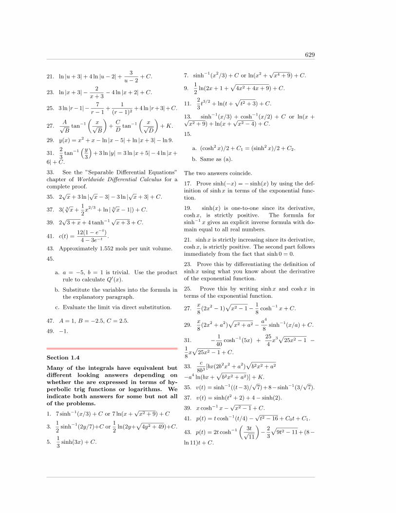
629
21. ln |u+ 3|+ 4 ln |u− 2|+ 3
u− 2+ C.
23. ln |x+ 3| − 2
x+ 3− 4 ln |x+ 2|+ C.
25. 3 ln |r−1|− 7
r − 1+
1
(r − 1)2+4 ln |r+3|+C.
27.A√B
tan−1
„x√B
«+C
Dtan−1
„x√D
«+K.
29. y(x) = x2 + x− ln |x− 5|+ ln |x+ 3| − ln 9.
31.2
3tan−1
“y3
”+ 3 ln |y| = 3 ln |x+ 5| − 4 ln |x+
6|+ C.
33. See the ”Separable Differential Equations”chapter of Worldwide Differential Calculus for acomplete proof.
35. 2√x+ 3 ln |
√x− 3| − 3 ln |
√x+ 3|+ C.
37. 3( 3√x+
1
2x2/3 + ln | 3
√x− 1|) + C.
39. 2√
3 + x+ 4 tanh−1√x+ 3 + C.
41. c(t) =12(1− e−t)
4− 3e−t.
43. Approximately 1.552 mols per unit volume.
45.
a. a = −5, b = 1 is trivial. Use the productrule to calculate Q′(x).
b. Substitute the variables into the formula inthe explanatory paragraph.
c. Evaluate the limit via direct substitution.
47. A = 1, B = −2.5, C = 2.5.
49. −1.
Section 1.4
Many of the integrals have equivalent butdifferent looking answers depending onwhether the are expressed in terms of hy-perbolic trig functions or logarithms. Weindicate both answers for some but not allof the problems.
1. 7 sinh−1(x/3) + C or 7 ln(x+√x2 + 9) + C
3.1
2sinh−1(2y/7)+C or
1
2ln(2y+
p4y2 + 49)+C.
5.1
3sinh(3x) + C.
7. sinh−1(x2/3) + C or ln(x2 +√x4 + 9) + C.
9.1
2ln(2x+ 1 +
p4x2 + 4x+ 9) + C.
11.2
3t3/2 + ln(t+
pt2 + 3) + C.
13. sinh−1(x/3) + cosh−1(x/2) + C or ln(x +√x2 + 9) + ln(x+
√x2 − 4) + C.
15.
a. (cosh2 x)/2 + C1 = (sinh2 x)/2 + C2.
b. Same as (a).
The two answers coincide.
17. Prove sinh(−x) = − sinh(x) by using the def-inition of sinhx in terms of the exponential func-tion.
19. sinh(x) is one-to-one since its derivative,coshx, is strictly positive. The formula forsinh−1 x gives an explicit inverse formula with do-main equal to all real numbers.
21. sinhx is strictly increasing since its derivative,coshx, is strictly positive. The second part followsimmediately from the fact that sinh 0 = 0.
23. Prove this by differentiating the definition ofsinhx using what you know about the derivativeof the exponential function.
25. Prove this by writing sinhx and coshx interms of the exponential function.
27.x
8(2x2 − 1)
px2 − 1− 1
8cosh−1 x+ C.
29.x
8(2x2 + a2)
px2 + a2 − a4
8sinh−1(x/a) + C.
31. − 1
40cosh−1(5x) +
25
4x3p
25x2 − 1 −1
8xp
25x2 − 1 + C.
33.c
8b3[bx(2b2x2 + a2)
pb2x2 + a2
−a4 ln(bx+pb2x2 + a2)] +K.
35. v(t) = sinh−1((t−3)/√
7)+8− sinh−1(3/√
7).
37. v(t) = sinh(t2 + 2) + 4− sinh(2).
39. x cosh−1 x−√x2 − 1 + C.
41. p(t) = t cosh−1(t/4)−√t2 − 16 + C0t+ C1.
43. p(t) = 2t cosh−1
„3t√11
«− 2
3
p9t2 − 11 + (8−
ln 11)t+ C.
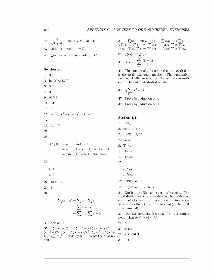
630 APPENDIX C. ANSWERS TO ODD-NUMBERED EXERCISES
45.x√
1 + x2= ln(t+
pt2 − 3) + C.
47. sinh−1 x− cosh−1 t = C.
49.1
2(sinx coshx+ cosx sinhx) + C.
Section 2.1
1. 85.
3. ln 120 ≈ 4.787.
5. 30.
7. 0.
9. 63/32.
11. 63.
13. 0.
15. ∆k2 = k2 − (k − 1)2 = 2k − 1.
17. 5.
19. 6k − 7.
21. 0.
23.
(∆f)(x) = sinx− sin(x− 1)
= sinx− (sinx cos 1− sin 1 cosx)
= (sinx)(1− cos 1) + sin 1 cosx.
25.
a. 1.
b. 0.
27. 100/101.
29. 1.
31. X(x− x) =
Xx−
Xx
=X
x− nx
=X
x−X
x = 0.
33. s ≈ 4.444.
35.P
(xi − x)2 =Px2i − 2x
Pxi +
Px2 =P
x2i − (2/n)
PxiPxi + (n/n2)(
Px)2 =
Px2i −
(1/n)(Pxi)
2. Divide by n − 1 to get the final re-sult.
37.P
(xi − x)(yi − y) =Pxiyi − x
Pyi =
yPxi +
Pxy =
Pxiyi − (2/n)
PxiPyi +
(n/n2)PxiPyi = (
Pxiyi)− (1/n)
PxiPyi.
39. f(m) =Pmi=1 i.
41. F (m) =
mXi=1
i(i+ 1)
2.
43. The number of gifts received on the m-th dayis the m-th triangular number. The cumulativenumber of gifts received by the end of the m-thday is the m-th tetrahedral number.
45.1
2
nXk=1
(u4 + 1).
47. Prove by induction on n.
49. Prove by induction on n.
Section 2.2
1. m(P) = 3.
3. m(P) = 1/4.
5. m(P) = 1/2n.
7. False.
9. True.
11. False.
13. False.
15.
a. Yes.
b. Yes.
17. 3250 meters.
19. 13/12 miles per hour.
21. Outline: the Riemann sum is telescoping. Thetotal displacement of a particle moving with con-stant velocity over an interval is equal to the ve-locity times the width of the interval (= the totaltime traveled).
23. Follows from the fact that if si is a samplepoint, then m ≤ f(si) ≤M .
25. 3.
27. 0.285.
29. ≈ 0.27683.
31. −π.
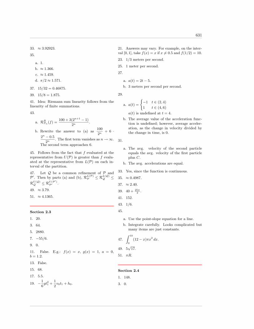
631
33. ≈ 3.92923.
35.
a. 1.
b. ≈ 1.366.
c. ≈ 1.459.
d. π/2 ≈ 1.571.
37. 15/32 = 0.46875.
39. 15/8 = 1.875.
41. Idea: Riemann sum linearity follows from thelinearity of finite summations.
43.
a. RRPn(f) =100 + 3(2n+1 − 1)
2n.
b. Rewrite the answer to (a) as100
2n+ 6 ·
2n − 0.5
2n. The first term vanishes as n→∞.
The second term approaches 6.
45. Follows from the fact that f evaluated at therepresentative from U(P) is greater than f evalu-ated at the representative from L(P) on each in-terval of the partition.
47. Let Q be a common refinement of P andP ′. Then by parts (a) and (b), RL(P)
P ≤ RL(Q)Q ≤
RU(Q)Q ≤ RU(P′)
P′ .
49. ≈ 3.79.
51. ≈ 4.1365.
Section 2.3
1. 20.
3. 64.
5. 2880.
7. −55/6.
9. 0.
11. False. E.g.: f(x) = x, g(x) = 1, a = 0,b = 1.2.
13. False.
15. 68.
17. 5.5.
19. −1
6gt21 +
1
2v0t1 + h0.
21. Answers may vary. For example, on the inter-val [0, 1], take f(x) = x if x 6= 0.5 and f(1/2) = 10.
23. 1/3 meters per second.
25. 1 meter per second.
27.
a. a(t) = 2t− 5.
b. 3 meters per second per second.
29.
a. a(t) =
(−1 t ∈ (2, 4)
1 t ∈ (4, 6)
a(t) is undefined at t = 4.
b. The average value of the acceleration func-tion is undefined; however, average acceler-ation, as the change in velocity divided bythe change in time, is 0.
31.
a. The avg. velocity of the second particleequals the avg. velocity of the first particleplus C.
b. The avg. accelerations are equal.
33. Yes, since the function is continuous.
35. ≈ 0.4987.
37. ≈ 2.40.
39. 40 + 25π2
.
41. 152.
43. 1/6.
45.
a. Use the point-slope equation for a line.
b. Integrate carefully. Looks complicated butmany items are just constants.
47.
Z 10
0
(12− x)πx2 dx.
49. 5√
17.
51. πR.
Section 2.4
1. 148.
3. 0.
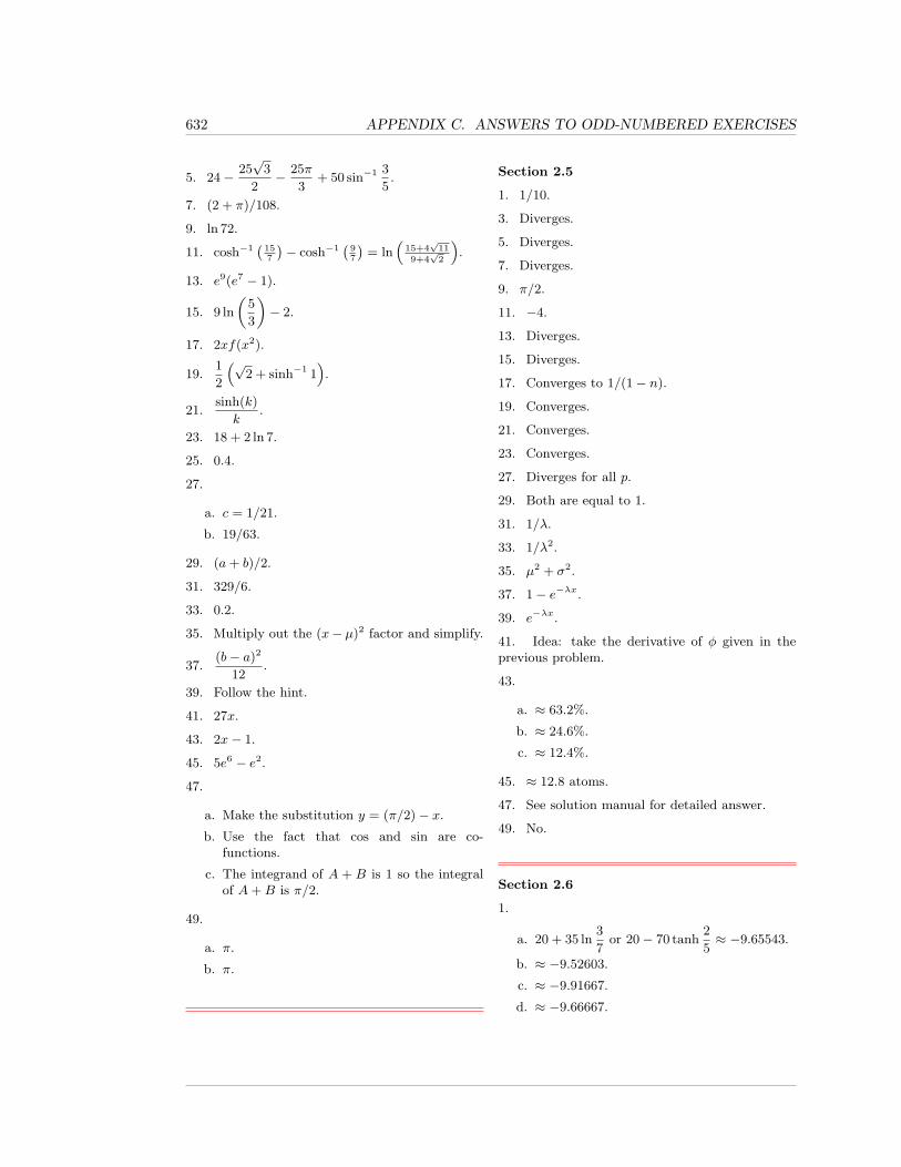
632 APPENDIX C. ANSWERS TO ODD-NUMBERED EXERCISES
5. 24− 25√
3
2− 25π
3+ 50 sin−1 3
5.
7. (2 + π)/108.
9. ln 72.
11. cosh−1`
157
´− cosh−1
`97
´= ln
“15+4
√11
9+4√
2
”.
13. e9(e7 − 1).
15. 9 ln
„5
3
«− 2.
17. 2xf(x2).
19.1
2
“√2 + sinh−1 1
”.
21.sinh(k)
k.
23. 18 + 2 ln 7.
25. 0.4.
27.
a. c = 1/21.
b. 19/63.
29. (a+ b)/2.
31. 329/6.
33. 0.2.
35. Multiply out the (x− µ)2 factor and simplify.
37.(b− a)2
12.
39. Follow the hint.
41. 27x.
43. 2x− 1.
45. 5e6 − e2.
47.
a. Make the substitution y = (π/2)− x.
b. Use the fact that cos and sin are co-functions.
c. The integrand of A + B is 1 so the integralof A+B is π/2.
49.
a. π.
b. π.
Section 2.5
1. 1/10.
3. Diverges.
5. Diverges.
7. Diverges.
9. π/2.
11. −4.
13. Diverges.
15. Diverges.
17. Converges to 1/(1− n).
19. Converges.
21. Converges.
23. Converges.
27. Diverges for all p.
29. Both are equal to 1.
31. 1/λ.
33. 1/λ2.
35. µ2 + σ2.
37. 1− e−λx.
39. e−λx.
41. Idea: take the derivative of φ given in theprevious problem.
43.
a. ≈ 63.2%.
b. ≈ 24.6%.
c. ≈ 12.4%.
45. ≈ 12.8 atoms.
47. See solution manual for detailed answer.
49. No.
Section 2.6
1.
a. 20 + 35 ln3
7or 20− 70 tanh
2
5≈ −9.65543.
b. ≈ −9.52603.
c. ≈ −9.91667.
d. ≈ −9.66667.
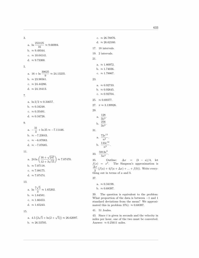
633
3.
a. ln253125
16≈ 9.66904.
b. ≈ 9.49344.
c. ≈ 10.04141.
d. ≈ 9.73300.
5.
a. 16 + ln30625
9≈ 24.13235.
b. ≈ 23.98561.
c. ≈ 24.44286.
d. ≈ 24.18413.
7.
a. ln 2/2 ≈ 0.34657.
b. ≈ 0.34248.
c. ≈ 0.35491.
d. ≈ 0.34726.
9.
a. −31
3+ ln 25 ≈ −7.11446.
b. ≈ −7.23043.
c. ≈ −6.87083.
d. ≈ −7.07685.
11.
a. 24 ln
„16 +
√247
12 + 3√
15
«≈ 7.07470.
b. ≈ 7.07118.
c. ≈ 7.08175.
d. ≈ 7.07474.
13.
a. ln7√
5
3≈ 1.65202.
b. ≈ 1.64581.
c. ≈ 1.66453.
d. ≈ 1.65243.
15.
a. 4.5`2√
5 + ln(2 +√
5)´≈ 26.62097.
b. ≈ 26.53705.
c. ≈ 26.78876.
d. ≈ 26.62160.
17. 18 intervals.
19. 2 intervals.
21.
a. ≈ 1.80972.
b. ≈ 1.74036.
c. ≈ 1.78867.
23.
a. ≈ 0.92733.
b. ≈ 0.92645.
c. ≈ 0.92704.
25. ≈ 0.69377.
27. π ≈ 3.139926.
29.
a.128
3n2.
b.256
3n2.
31.
a.72e12
n2.
b.144e12
n2.
33.5913e9
5n4.
35. Outline: ∆x = (b − a)/4, letf(x) = x2. The Simpson’s approximation is∆x
3(f(a) + 4f(a+ ∆x) + ...+ f(b)). Write every-
thing out in terms of a and b.
37.
a. ≈ 0.34198.
b. ≈ 0.68397.
39. The question is equivalent to the problem:What proportion of the data is between −1 and 1standard deviations from the mean? We approxi-mated this in problem 37b): ≈ 0.68397.
41. 51 Joules.
43. Since t is given in seconds and the velocity inmiles per hour, one of the two must be converted.Answer: ≈ 0.25611 miles.
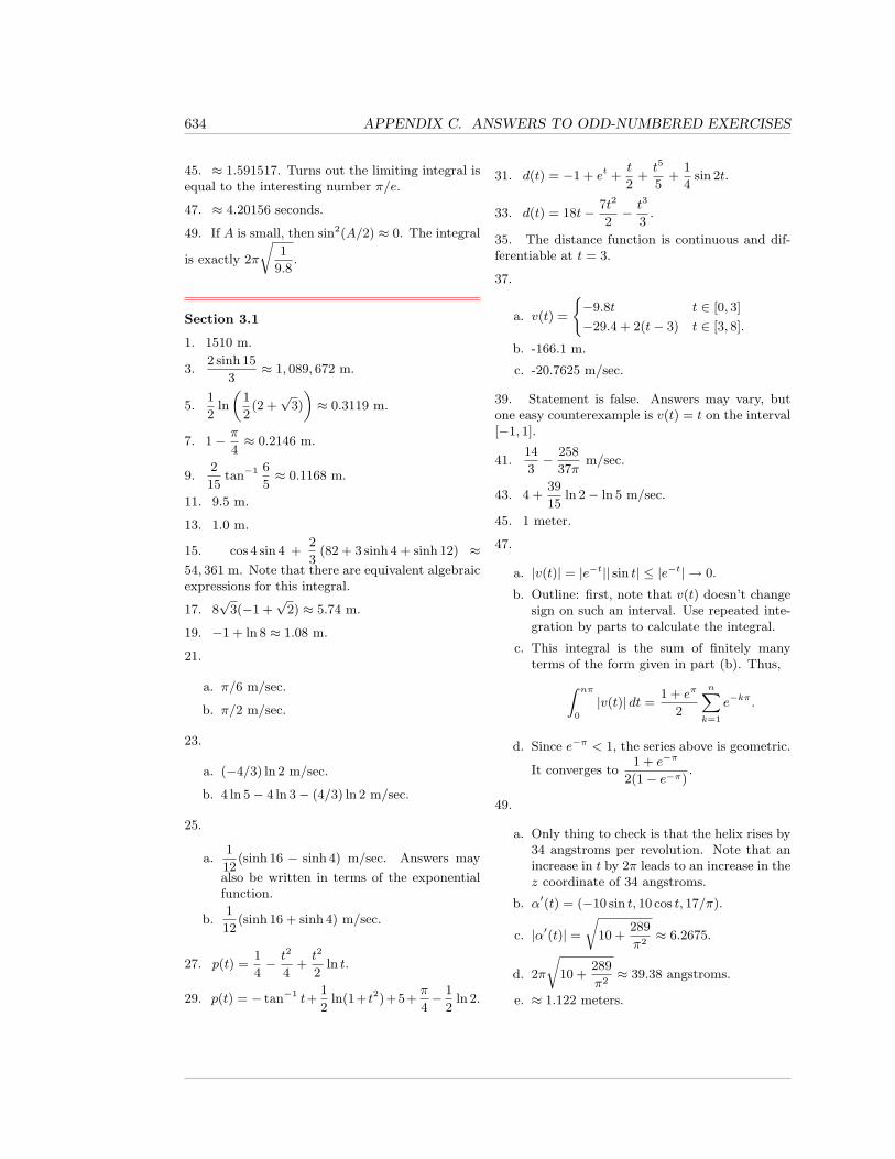
634 APPENDIX C. ANSWERS TO ODD-NUMBERED EXERCISES
45. ≈ 1.591517. Turns out the limiting integral isequal to the interesting number π/e.
47. ≈ 4.20156 seconds.
49. If A is small, then sin2(A/2) ≈ 0. The integral
is exactly 2π
r1
9.8.
Section 3.1
1. 1510 m.
3.2 sinh 15
3≈ 1, 089, 672 m.
5.1
2ln
„1
2(2 +
√3)
«≈ 0.3119 m.
7. 1− π
4≈ 0.2146 m.
9.2
15tan−1 6
5≈ 0.1168 m.
11. 9.5 m.
13. 1.0 m.
15. cos 4 sin 4 +2
3(82 + 3 sinh 4 + sinh 12) ≈
54, 361 m. Note that there are equivalent algebraicexpressions for this integral.
17. 8√
3(−1 +√
2) ≈ 5.74 m.
19. −1 + ln 8 ≈ 1.08 m.
21.
a. π/6 m/sec.
b. π/2 m/sec.
23.
a. (−4/3) ln 2 m/sec.
b. 4 ln 5− 4 ln 3− (4/3) ln 2 m/sec.
25.
a.1
12(sinh 16 − sinh 4) m/sec. Answers may
also be written in terms of the exponentialfunction.
b.1
12(sinh 16 + sinh 4) m/sec.
27. p(t) =1
4− t2
4+t2
2ln t.
29. p(t) = − tan−1 t+1
2ln(1+ t2)+5+
π
4− 1
2ln 2.
31. d(t) = −1 + et +t
2+t5
5+
1
4sin 2t.
33. d(t) = 18t− 7t2
2− t3
3.
35. The distance function is continuous and dif-ferentiable at t = 3.
37.
a. v(t) =
(−9.8t t ∈ [0, 3]
−29.4 + 2(t− 3) t ∈ [3, 8].
b. -166.1 m.
c. -20.7625 m/sec.
39. Statement is false. Answers may vary, butone easy counterexample is v(t) = t on the interval[−1, 1].
41.14
3− 258
37πm/sec.
43. 4 +39
15ln 2− ln 5 m/sec.
45. 1 meter.
47.
a. |v(t)| = |e−t|| sin t| ≤ |e−t| → 0.
b. Outline: first, note that v(t) doesn’t changesign on such an interval. Use repeated inte-gration by parts to calculate the integral.
c. This integral is the sum of finitely manyterms of the form given in part (b). Thus,Z nπ
0
|v(t)| dt =1 + eπ
2
nXk=1
e−kπ.
d. Since e−π < 1, the series above is geometric.
It converges to1 + e−π
2(1− e−π).
49.
a. Only thing to check is that the helix rises by34 angstroms per revolution. Note that anincrease in t by 2π leads to an increase in thez coordinate of 34 angstroms.
b. α′(t) = (−10 sin t, 10 cos t, 17/π).
c. |α′(t)| =r
10 +289
π2≈ 6.2675.
d. 2π
r10 +
289
π2≈ 39.38 angstroms.
e. ≈ 1.122 meters.
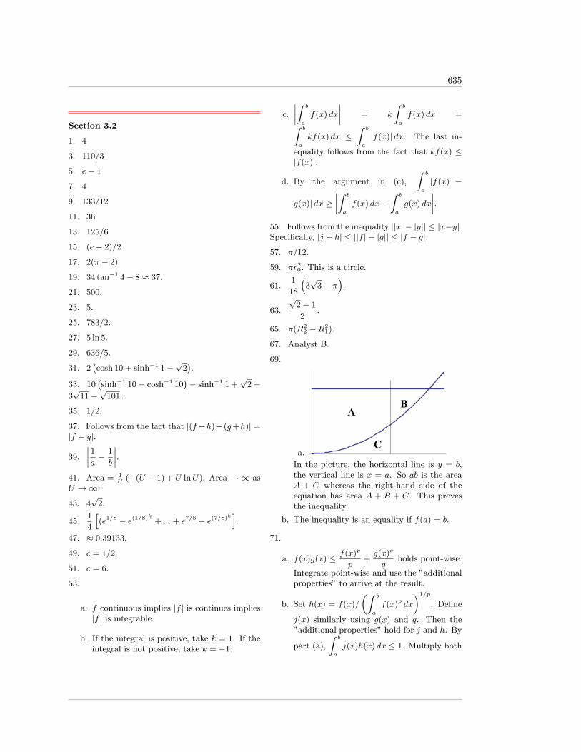
635
Section 3.2
1. 4
3. 110/3
5. e− 1
7. 4
9. 133/12
11. 36
13. 125/6
15. (e− 2)/2
17. 2(π − 2)
19. 34 tan−1 4− 8 ≈ 37.
21. 500.
23. 5.
25. 783/2.
27. 5 ln 5.
29. 636/5.
31. 2`cosh 10 + sinh−1 1−
√2´.
33. 10`sinh−1 10− cosh−1 10
´− sinh−1 1 +
√2 +
3√
11−√
101.
35. 1/2.
37. Follows from the fact that |(f+h)−(g+h)| =|f − g|.
39.
˛1
a− 1
b
˛.
41. Area = 1U
(−(U − 1) + U lnU). Area →∞ asU →∞.
43. 4√
2.
45.1
4
h(e1/8 − e(1/8)
k
+ ...+ e7/8 − e(7/8)ki.
47. ≈ 0.39133.
49. c = 1/2.
51. c = 6.
53.
a. f continuous implies |f | is continues implies|f | is integrable.
b. If the integral is positive, take k = 1. If theintegral is not positive, take k = −1.
c.
˛Z b
a
f(x) dx
˛= k
Z b
a
f(x) dx =Z b
a
kf(x) dx ≤Z b
a
|f(x)| dx. The last in-
equality follows from the fact that kf(x) ≤|f(x)|.
d. By the argument in (c),
Z b
a
|f(x) −
g(x)| dx ≥˛Z b
a
f(x) dx−Z b
a
g(x) dx
˛.
55. Follows from the inequality ||x| − |y|| ≤ |x−y|.Specifically, |j − h| ≤ ||f | − |g|| ≤ |f − g|.
57. π/12.
59. πr20. This is a circle.
61.1
18
“3√
3− π”
.
63.
√2− 1
2.
65. π(R22 −R2
1).
67. Analyst B.
69.
a.
B
C
A
In the picture, the horizontal line is y = b,the vertical line is x = a. So ab is the areaA + C whereas the right-hand side of theequation has area A + B + C. This provesthe inequality.
b. The inequality is an equality if f(a) = b.
71.
a. f(x)g(x) ≤ f(x)p
p+g(x)q
qholds point-wise.
Integrate point-wise and use the ”additionalproperties” to arrive at the result.
b. Set h(x) = f(x)/
„Z b
a
f(x)p dx
«1/p
. Define
j(x) similarly using g(x) and q. Then the”additional properties” hold for j and h. By
part (a),
Z b
a
j(x)h(x) dx ≤ 1. Multiply both
636 APPENDIX C. ANSWERS TO ODD-NUMBERED EXERCISES
sides of the equation by the denominators ofh and j to arrive at the inequality.
Section 3.3
1. (0, 0, 8).
3. (110,−90, 220).
5. (9, 9, 9).
7. No, the derivative is the zero vector when t = 0.
9. Yes. The map avoids the cusp at t = −2.
11. No, the derivative is the zero vector whent = 0.
13. ~w(s) = (3 +6s√62, 2− 5s√
62, 7 +
s√62
).
15. Follows from the fact that
˛˛d~φds
˛˛ = 1 for all
s ∈ [a, b].
17.π√
2
4.
19. 2(−1 + (1 + π)3/2).
21. ln(1 +√
2).
23. 5√
2−√
26 + 5 ln5 +√
26
1 +√
2.
25.7
6√a
+
√a
4.
27. ~p(s) = (a cos sa2+b2
, a sin sa2+b2
,,b cos s
a2+b2, b sin s
a2+b2).
29. It is not regular as it fails to be differentiableat t = 0. It is not rectifiable since it is not one-to-one on any open interval containing zero.
31.
a. Let ~p(t) = R(sin t, 0, cos t) for t ∈ [0, π/2],R(cos(t − π
2), sin(t − π
2, 0) for t ∈ [π/2, π]
and R(0,− cos t,− sin t) for t ∈ [π, 3π2
].
b. 3πR/2.
33.
a. Apply the chain rule to φ(t) = ψ(f(t)).
b. Use part (a) and the Substitution Rule.Also, since φ(a) = ψ(c), and all the functions
are one-to-one, it must be that |dudt| > 0.
35. 8r.
37. ~p ′(ψ) = r2(r1+r2)r1
·“cos r2ψ
r1− cos (r1+r2)ψ
r1,− sin r2ψ
r1+ sin (r1+r2)ψ
r1
”.
39. Idea: cusps occur whenever ψ = 2nπ, n an in-teger. The cusps therefore occur, in terms of θ, atθ = (r2/r1)(2nπ). When r2/r1 is irrational, cuspswill start repeating themselves at a frequency con-trolled by r1. However, if r2/r1 is irrational, thenfor an arbitrary θ we can find an n such (r2/r1)2nπis arbitrarily close to θ.
41. x′(θ) = (r2−r1) sin θ+(r2−r1) sin(r1 − r2)θ
r2.
y′(θ) = (r1 − r2) cos θ + (r2 − r1) cos(r1 − r2)θ
r2.
43.
a. Let f(t) = ~c(t) · ~v. Then f ′(t) = ~c ′ · ~v. Usethis fact and Fundamental Theorem of Cal-culus to obtain the result.
b. Use the hint and the fact that ~v is a unitvector. I.e., |~v| = 1.
c.
Z b
a
|~c ′(t)| dt ≥Z b
a
~c ′ · ~v dt =
(p− q) · (p− q)|p− q| = |p− q|.
45.
a.dx
dθ= r′(θ) cos θ − r(θ) sin θ,
dy
dθ=
r′(θ) sin θ + r(θ) cos θ.
b. Follows from the fact that x′(θ)2 + y′(θ)2 =r(θ)2 + r′(θ)2.
47. 2πC. This is a circle.
49. πp
1 + 4π2 +1
2sinh−1 2π.
Section 3.4
1.
a. 4/3.
b. y = x2.
3.
a. 1/5.
b. x2 = y3.
5.
637
a. (1/2)(−8 + 23 + ln 27).
b. x = ln y.
7. 3π/2.
9. 33π.
11. 6π.
13.3√
3
4+π
4.
15. 5/2.
Section 3.5
1. 58.
3. 1/4.
5. 800/3.
7.1
3
„a3
h− b4a
h
«.
9. π/8.
11. 1574π/15.
13. π/5.
15.π
2n+ 1.
17.π(16− π)
2.
19. 6929π/16.
21.3√
3π
16.
23. ≈ 6.45.
25. ≈ 1.1063.
27. ≈ 22.4981.
29. 2π
„1
n+ 2− 1
m+ 2
«.
31. B/3.
33. The integral is finite by comparison withGabriel’s Horn.
35. ≈ 5.23016.
37. 2π2Rr2.
39. 2π2.
41. 4750π/3 cm3.
43. ≈ 27.672 cm.
45. 2π(1− a). The integral converges to 2π.
47. Vc =3c(16/3)
10.
49. π2(R2 − r2)/3.
51. π.
53.
a. π.
b. The integral converges to 2π.
c. The integral converges to 2π.
55. The volumes of a right circular cone, hemi-sphere, cylinder and sphere are πr2h/3, 2πr2h/3,πr2h, and 4πr2h/3 respectively.
Section 3.6
1. 152π√
10.
3. π(eπp
1 + e2π −√
2 + sinh−1 eπ − sinh−1 1).
5.π
6
“37√
37− 1”
.
7. 33π√
5.
9.5π
27
“29√
145− 2√
10”
.
11. 2π (4 sinh 4− cosh 4 + 1).
13. 16π√
10.
15.π
6
“1 +√
5 + 3 sinh−1 2”
.
17. π|m|√
1 +m2.
19. ≈ 8496.
21. ≈ 150.8.
23. ≈ 3.395.
25. A =
Z b
a
2π (f(x)− y0)
q1 + [f ′(x)]2 dx.
27. A =
Z b
a
2π (x− x0))
q1 + [f ′(x)]2 dx.
29.πa
6
h(a2 + 4b+ 4)3/2 − (a2 + 4b)3/2
i.
31.
a. S(m) =
(πa√
1 +m2 m 6= 0
0 m = 0.
b. S is neither continuous nor differentiable atm = 0.
33.
a. 3π.
638 APPENDIX C. ANSWERS TO ODD-NUMBERED EXERCISES
b. Annulus.
35. One way to do this is to write the equationperpendicular to y = mx passing through (x1, y1).Find where the two lines intersect and use the dis-tance formula.
37. A =
Z c
a
2π|f(x)−mx− b|√
1 +m2
p1 + f ′(x)2 dx.
39.
a. A =R ca
2πf(x)p
1 + f ′(x)2 dx. Here we as-sume f(x) > 0.
b. A =
√2
2
Z c
a
2π(f(x) − x)p
1 + f ′(x)2 dx.
We assume f(x) > x, or that f lies aboutthe line y = x.
c. A =
Z c
a
2πxp
1 + f ′(x)2 dx. We assume
x > 0.
41. 16π.
43. 16π.
45.
Z 5
2
2πex − 3x√
10·p
1 + e2x dx.
47.2π√
5
Z 4
2
„2x− x+ 2
x+ 1
«s1 +
1
(1 + x)4dx.
49.2π
17
Z 8
3
(4x−√x+ 1)
r1 +
1
4 + 4xdx.
Section 3.7
1. 18 sinh 5.
3. 720π.
5. 83, 592π/5.
7. 3456π/35.
9.
Z y0/m
0
δ(x)2πx(y0 −mx) dx.
11. 2πh
Z b
0
xδ(x) dx.
13. 2π(49 ln 49− 25 ln 25− 24).
15.
a. 36.
b. x = −7 +√
85.
17.
a. 1.
b. x = π/3.
19.
a. 2 sinh 1.
b. x = 0.
21. x = ln
„1
2(e10 − 1) + 1
«.
23.108 + 9π
4.
25. 45/2.
27. ≈ 14.689 kg.
29. c = 6/5.
31. 22.5 kg/m3.
33. Numerator follows from comments in thischapter. Denominator follows from the shell vol-ume formula.
35. 103.4 kg/m3.
37.
a. 117π/t.
b. −117π/t2.
39. π(t − 1)2 (16 + 9 ln 9(ln 9− 2)) +3πt(ln 9)2 ln 81.
41. 2π(5 + ln 6).
43. rπe4(e32 − 1).
45. 783/2.
47.1
2(e6 − 1)(e5 − 1).
49. 844/3.
Section 3.8
1. (4/19, 10/19).
3. (3, 3).
5. (2/27,−1/9,−2/9).
7.
a. 25225/12.
b. 1009/192.
9.
a.2
27(660 + 7 ln(17/5)).
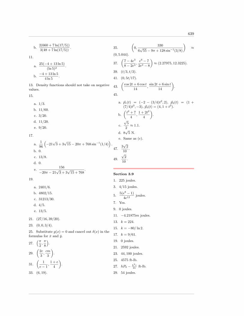
639
b.2(660 + 7 ln(17/5))
3(48 + 7 ln(17/5)).
11.
a.25(−4 + 13 ln 5)
(ln 5)2.
b.−4 + 13 ln 5
4 ln 5.
13. Density functions should not take on negativevalues.
15.
a. 1/3.
b. 11/60.
c. 3/20.
d. 11/20.
e. 9/20.
17.
a.1
96
“−21√
3 + 3√
15− 20π + 768 sin−1(1/4)”.
b. 0.
c. 13/8.
d. 0.
e.156
−20π − 21√
3 + 3√
15 + 768.
19.
a. 2401/6.
b. 4802/15.
c. 31213/30.
d. 4/5.
e. 13/5.
21. (27/16, 39/20).
23. (0, 0, 3/4).
25. Substitute g(x) = 0 and cancel out δ(x) in theformulas for x and y.
27.“π
2,π
8
”.
29.
„2c
3,cm
3
«.
31.
„1
e− 1,
1 + e
4
«.
33. (6, 19).
35.
„0,
330
6√
55− 9π + 128 sin−1(3/8)
«≈
(0, 5.044).
37.
„7− 4e3
8− 2e3,e6 − 7
2e3 − 8
«≈ (2.27975, 12.3225).
39. (t/3, t/3).
41. (0, 5t/17).
43.
„cos 2t+ 6 cos t
14,
sin 2t+ 6 sin t
14
«.
45.
a. ~p1(t) = (−2 − (3/4)t2, 2), ~p2(t) = (1 +(7/4)t2,−3), ~p3(t) = (4, 1 + t2).
b.
„t2 + 7
4,
1 + 2t2
4
«.
c.
√5
2≈ 1.1.
d. 8√
5 N.
e. Same as (c).
47.3√
2
10.
49.
√2
10.
Section 3.9
1. 225 joules.
3. 4/15 joules.
5.5(e8 − 1)
4e12joules.
7. Yes.
9. 0 joules.
11. −4.21875m joules.
13. k = 224.
15. k = −80/ ln 2.
17. k = 9/61.
19. 0 joules.
21. 2592 joules.
23. 44, 100 joules.
25. 4575 ft-lb.
27. hP0 − h2r2v
ft-lb.
29. 54 joules.
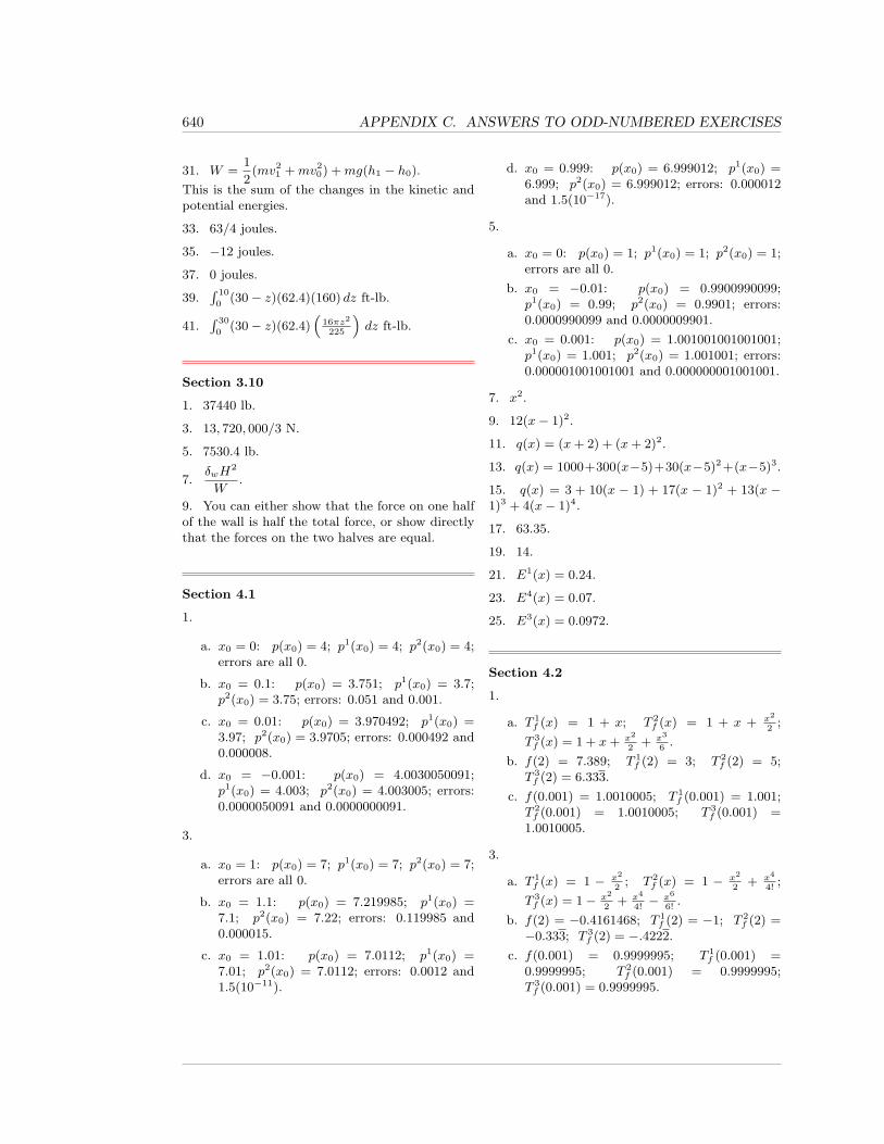
640 APPENDIX C. ANSWERS TO ODD-NUMBERED EXERCISES
31. W =1
2(mv2
1 +mv20) +mg(h1 − h0).
This is the sum of the changes in the kinetic andpotential energies.
33. 63/4 joules.
35. −12 joules.
37. 0 joules.
39.R 10
0(30− z)(62.4)(160) dz ft-lb.
41.R 30
0(30− z)(62.4)
“16πz2
225
”dz ft-lb.
Section 3.10
1. 37440 lb.
3. 13, 720, 000/3 N.
5. 7530.4 lb.
7.δwH
2
W.
9. You can either show that the force on one halfof the wall is half the total force, or show directlythat the forces on the two halves are equal.
Section 4.1
1.
a. x0 = 0: p(x0) = 4; p1(x0) = 4; p2(x0) = 4;errors are all 0.
b. x0 = 0.1: p(x0) = 3.751; p1(x0) = 3.7;p2(x0) = 3.75; errors: 0.051 and 0.001.
c. x0 = 0.01: p(x0) = 3.970492; p1(x0) =3.97; p2(x0) = 3.9705; errors: 0.000492 and0.000008.
d. x0 = −0.001: p(x0) = 4.0030050091;p1(x0) = 4.003; p2(x0) = 4.003005; errors:0.0000050091 and 0.0000000091.
3.
a. x0 = 1: p(x0) = 7; p1(x0) = 7; p2(x0) = 7;errors are all 0.
b. x0 = 1.1: p(x0) = 7.219985; p1(x0) =7.1; p2(x0) = 7.22; errors: 0.119985 and0.000015.
c. x0 = 1.01: p(x0) = 7.0112; p1(x0) =7.01; p2(x0) = 7.0112; errors: 0.0012 and1.5(10−11).
d. x0 = 0.999: p(x0) = 6.999012; p1(x0) =6.999; p2(x0) = 6.999012; errors: 0.000012and 1.5(10−17).
5.
a. x0 = 0: p(x0) = 1; p1(x0) = 1; p2(x0) = 1;errors are all 0.
b. x0 = −0.01: p(x0) = 0.9900990099;p1(x0) = 0.99; p2(x0) = 0.9901; errors:0.0000990099 and 0.0000009901.
c. x0 = 0.001: p(x0) = 1.001001001001001;p1(x0) = 1.001; p2(x0) = 1.001001; errors:0.000001001001001 and 0.000000001001001.
7. x2.
9. 12(x− 1)2.
11. q(x) = (x+ 2) + (x+ 2)2.
13. q(x) = 1000+300(x−5)+30(x−5)2+(x−5)3.
15. q(x) = 3 + 10(x − 1) + 17(x − 1)2 + 13(x −1)3 + 4(x− 1)4.
17. 63.35.
19. 14.
21. E1(x) = 0.24.
23. E4(x) = 0.07.
25. E3(x) = 0.0972.
Section 4.2
1.
a. T 1f (x) = 1 + x; T 2
f (x) = 1 + x + x2
2;
T 3f (x) = 1 + x+ x2
2+ x3
6.
b. f(2) = 7.389; T 1f (2) = 3; T 2
f (2) = 5;T 3f (2) = 6.333.
c. f(0.001) = 1.0010005; T 1f (0.001) = 1.001;
T 2f (0.001) = 1.0010005; T 3
f (0.001) =1.0010005.
3.
a. T 1f (x) = 1 − x2
2; T 2
f (x) = 1 − x2
2+ x4
4!;
T 3f (x) = 1− x2
2+ x4
4!− x6
6!.
b. f(2) = −0.4161468; T 1f (2) = −1; T 2
f (2) =−0.333; T 3
f (2) = −.4222.
c. f(0.001) = 0.9999995; T 1f (0.001) =
0.9999995; T 2f (0.001) = 0.9999995;
T 3f (0.001) = 0.9999995.
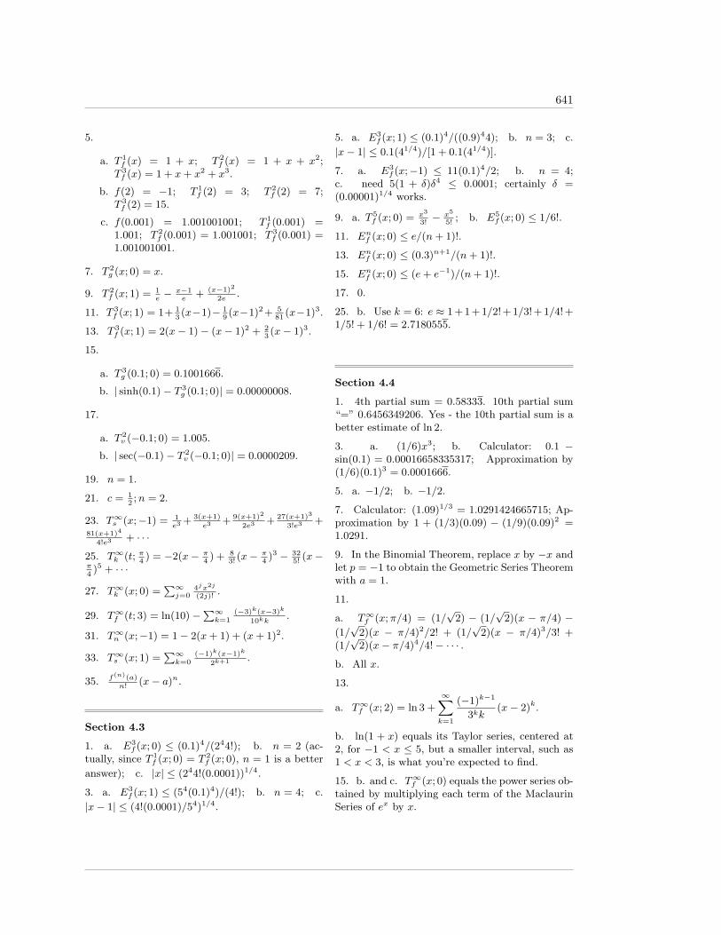
641
5.
a. T 1f (x) = 1 + x; T 2
f (x) = 1 + x + x2;T 3f (x) = 1 + x+ x2 + x3.
b. f(2) = −1; T 1f (2) = 3; T 2
f (2) = 7;T 3f (2) = 15.
c. f(0.001) = 1.001001001; T 1f (0.001) =
1.001; T 2f (0.001) = 1.001001; T 3
f (0.001) =1.001001001.
7. T 2g (x; 0) = x.
9. T 2f (x; 1) = 1
e− x−1
e+ (x−1)2
2e.
11. T 3f (x; 1) = 1+ 1
3(x−1)− 1
9(x−1)2+ 5
81(x−1)3.
13. T 3f (x; 1) = 2(x− 1)− (x− 1)2 + 2
3(x− 1)3.
15.
a. T 3g (0.1; 0) = 0.1001666.
b. | sinh(0.1)− T 3g (0.1; 0)| = 0.00000008.
17.
a. T 2v (−0.1; 0) = 1.005.
b. | sec(−0.1)− T 2v (−0.1; 0)| = 0.0000209.
19. n = 1.
21. c = 12;n = 2.
23. T∞s (x;−1) = 1e3
+ 3(x+1)
e3+ 9(x+1)2
2e3+ 27(x+1)3
3!e3+
81(x+1)4
4!e3+ · · ·
25. T∞k (t; π4
) = −2(x− π4
) + 83!
(x− π4
)3 − 325!
(x−π4
)5 + · · ·
27. T∞k (x; 0) =P∞j=0
4jx2j
(2j)!.
29. T∞f (t; 3) = ln(10)−P∞k=1
(−3)k(x−3)k
10kk.
31. T∞n (x;−1) = 1− 2(x+ 1) + (x+ 1)2.
33. T∞s (x; 1) =P∞k=0
(−1)k(x−1)k
2k+1 .
35. f(n)(a)n!
(x− a)n.
Section 4.3
1. a. E3f (x; 0) ≤ (0.1)4/(244!); b. n = 2 (ac-
tually, since T 1f (x; 0) = T 2
f (x; 0), n = 1 is a better
answer); c. |x| ≤ (244!(0.0001))1/4.
3. a. E3f (x; 1) ≤ (54(0.1)4)/(4!); b. n = 4; c.
|x− 1| ≤ (4!(0.0001)/54)1/4.
5. a. E3f (x; 1) ≤ (0.1)4/((0.9)44); b. n = 3; c.
|x− 1| ≤ 0.1(41/4)/[1 + 0.1(41/4)].
7. a. E3f (x;−1) ≤ 11(0.1)4/2; b. n = 4;
c. need 5(1 + δ)δ4 ≤ 0.0001; certainly δ =(0.00001)1/4 works.
9. a. T 5f (x; 0) = x3
3!− x5
5!; b. E5
f (x; 0) ≤ 1/6!.
11. Enf (x; 0) ≤ e/(n+ 1)!.
13. Enf (x; 0) ≤ (0.3)n+1/(n+ 1)!.
15. Enf (x; 0) ≤ (e+ e−1)/(n+ 1)!.
17. 0.
25. b. Use k = 6: e ≈ 1 + 1 + 1/2! + 1/3! + 1/4! +1/5! + 1/6! = 2.7180555.
Section 4.4
1. 4th partial sum = 0.58333. 10th partial sum“=” 0.6456349206. Yes - the 10th partial sum is abetter estimate of ln 2.
3. a. (1/6)x3; b. Calculator: 0.1 −sin(0.1) = 0.00016658335317; Approximation by(1/6)(0.1)3 = 0.0001666.
5. a. −1/2; b. −1/2.
7. Calculator: (1.09)1/3 = 1.0291424665715; Ap-proximation by 1 + (1/3)(0.09) − (1/9)(0.09)2 =1.0291.
9. In the Binomial Theorem, replace x by −x andlet p = −1 to obtain the Geometric Series Theoremwith a = 1.
11.
a. T∞f (x;π/4) = (1/√
2) − (1/√
2)(x − π/4) −(1/√
2)(x − π/4)2/2! + (1/√
2)(x − π/4)3/3! +(1/√
2)(x− π/4)4/4!− · · · .
b. All x.
13.
a. T∞f (x; 2) = ln 3 +
∞Xk=1
(−1)k−1
3kk(x− 2)k.
b. ln(1 + x) equals its Taylor series, centered at2, for −1 < x ≤ 5, but a smaller interval, such as1 < x < 3, is what you’re expected to find.
15. b. and c. T∞f (x; 0) equals the power series ob-tained by multiplying each term of the MaclaurinSeries of ex by x.
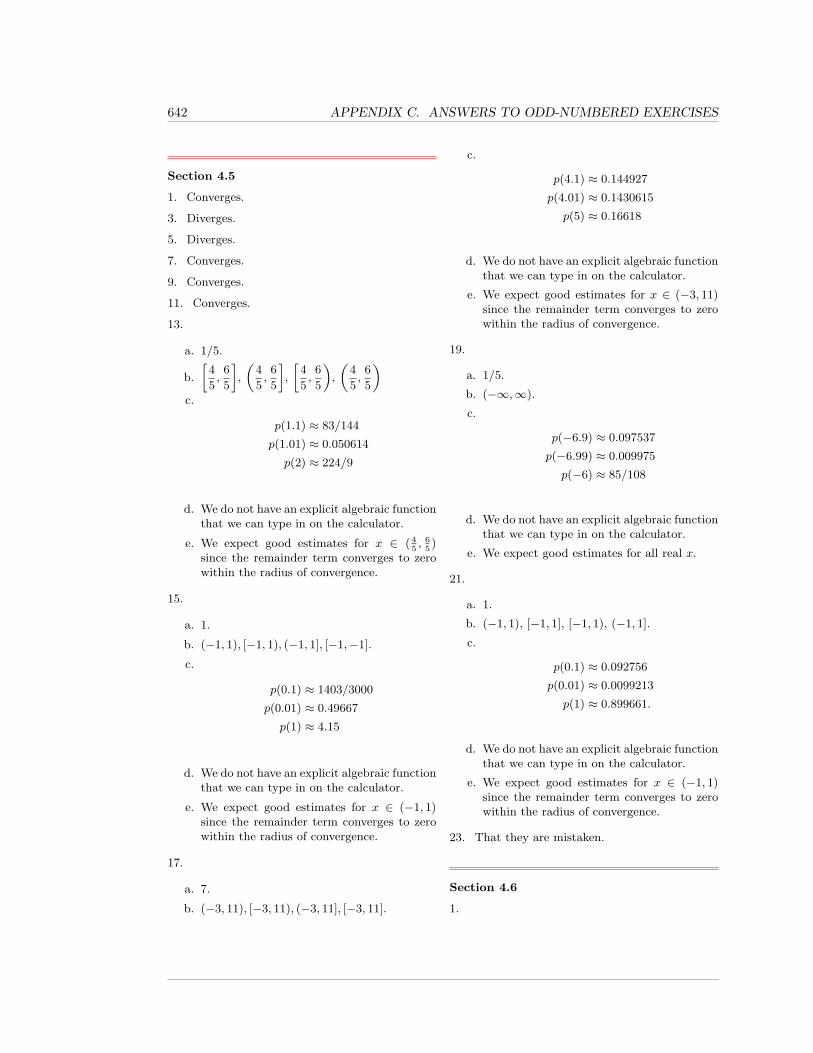
642 APPENDIX C. ANSWERS TO ODD-NUMBERED EXERCISES
Section 4.5
1. Converges.
3. Diverges.
5. Diverges.
7. Converges.
9. Converges.
11. Converges.
13.
a. 1/5.
b.
»4
5,
6
5
–,
„4
5,
6
5
–,
»4
5,
6
5
«,
„4
5,
6
5
«c.
p(1.1) ≈ 83/144
p(1.01) ≈ 0.050614
p(2) ≈ 224/9
d. We do not have an explicit algebraic functionthat we can type in on the calculator.
e. We expect good estimates for x ∈ ( 45, 6
5)
since the remainder term converges to zerowithin the radius of convergence.
15.
a. 1.
b. (−1, 1), [−1, 1), (−1, 1], [−1,−1].
c.
p(0.1) ≈ 1403/3000
p(0.01) ≈ 0.49667
p(1) ≈ 4.15
d. We do not have an explicit algebraic functionthat we can type in on the calculator.
e. We expect good estimates for x ∈ (−1, 1)since the remainder term converges to zerowithin the radius of convergence.
17.
a. 7.
b. (−3, 11), [−3, 11), (−3, 11], [−3, 11].
c.
p(4.1) ≈ 0.144927
p(4.01) ≈ 0.1430615
p(5) ≈ 0.16618
d. We do not have an explicit algebraic functionthat we can type in on the calculator.
e. We expect good estimates for x ∈ (−3, 11)since the remainder term converges to zerowithin the radius of convergence.
19.
a. 1/5.
b. (−∞,∞).
c.
p(−6.9) ≈ 0.097537
p(−6.99) ≈ 0.009975
p(−6) ≈ 85/108
d. We do not have an explicit algebraic functionthat we can type in on the calculator.
e. We expect good estimates for all real x.
21.
a. 1.
b. (−1, 1), [−1, 1], [−1, 1), (−1, 1].
c.
p(0.1) ≈ 0.092756
p(0.01) ≈ 0.0099213
p(1) ≈ 0.899661.
d. We do not have an explicit algebraic functionthat we can type in on the calculator.
e. We expect good estimates for x ∈ (−1, 1)since the remainder term converges to zerowithin the radius of convergence.
23. That they are mistaken.
Section 4.6
1.
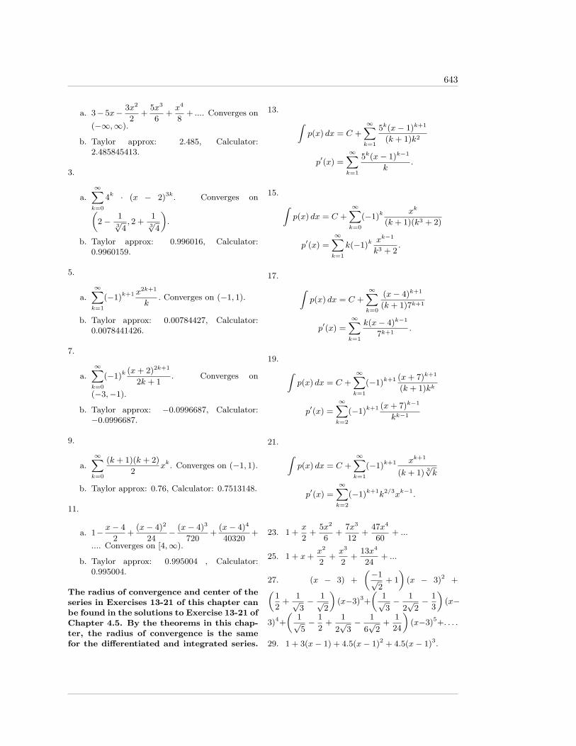
643
a. 3− 5x− 3x2
2+
5x3
6+x4
8+ .... Converges on
(−∞,∞).
b. Taylor approx: 2.485, Calculator:2.485845413.
3.
a.
∞Xk=0
4k · (x − 2)3k. Converges on„2− 1
3√
4, 2 +
13√
4
«.
b. Taylor approx: 0.996016, Calculator:0.9960159.
5.
a.
∞Xk=1
(−1)k+1 x2k+1
k. Converges on (−1, 1).
b. Taylor approx: 0.00784427, Calculator:0.0078441426.
7.
a.
∞Xk=0
(−1)k(x+ 2)2k+1
2k + 1. Converges on
(−3,−1).
b. Taylor approx: −0.0996687, Calculator:−0.0996687.
9.
a.
∞Xk=0
(k + 1)(k + 2)
2xk. Converges on (−1, 1).
b. Taylor approx: 0.76, Calculator: 0.7513148.
11.
a. 1− x− 4
2+
(x− 4)2
24− (x− 4)3
720+
(x− 4)4
40320+
.... Converges on [4,∞).
b. Taylor approx: 0.995004 , Calculator:0.995004.
The radius of convergence and center of theseries in Exercises 13-21 of this chapter canbe found in the solutions to Exercise 13-21 ofChapter 4.5. By the theorems in this chap-ter, the radius of convergence is the samefor the differentiated and integrated series.
13. Zp(x) dx = C +
∞Xk=1
5k(x− 1)k+1
(k + 1)k2
p′(x) =
∞Xk=1
5k(x− 1)k−1
k.
15. Zp(x) dx = C +
∞Xk=0
(−1)kxk
(k + 1)(k3 + 2)
p′(x) =
∞Xk=1
k(−1)kxk−1
k3 + 2.
17. Zp(x) dx = C +
∞Xk=0
(x− 4)k+1
(k + 1)7k+1
p′(x) =
∞Xk=1
k(x− 4)k−1
7k+1.
19. Zp(x) dx = C +
∞Xk=1
(−1)k+1 (x+ 7)k+1
(k + 1)kk
p′(x) =
∞Xk=2
(−1)k+1 (x+ 7)k−1
kk−1
21. Zp(x) dx = C +
∞Xk=1
(−1)k+1 xk+1
(k + 1) 3√k
p′(x) =
∞Xk=2
(−1)k+1k2/3xk−1.
23. 1 +x
2+
5x2
6+
7x3
12+
47x4
60+ ...
25. 1 + x+x2
2+x3
2+
13x4
24+ ...
27. (x − 3) +
„−1√
2+ 1
«(x − 3)2 +„
1
2+
1√3− 1√
2
«(x−3)3+
„1√3− 1
2√
2− 1
3
«(x−
3)4+
„1√5− 1
2+
1
2√
3− 1
6√
2+
1
24
«(x−3)5+. . . .
29. 1 + 3(x− 1) + 4.5(x− 1)2 + 4.5(x− 1)3.
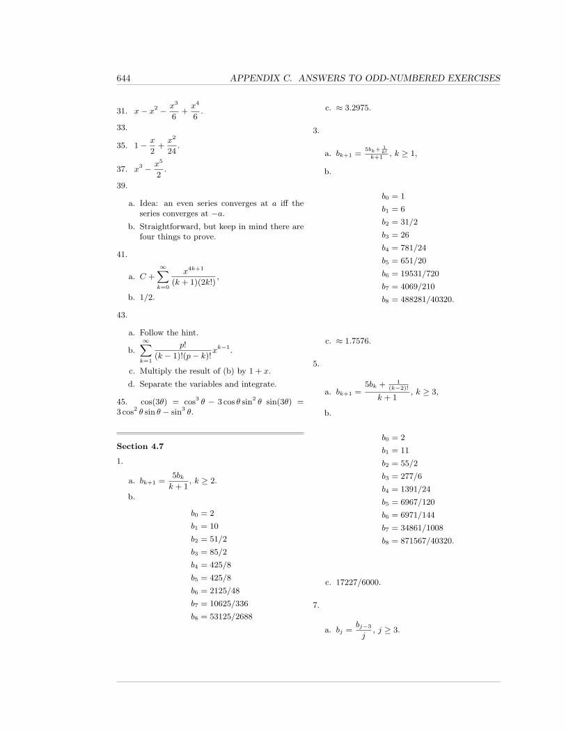
644 APPENDIX C. ANSWERS TO ODD-NUMBERED EXERCISES
31. x− x2 − x3
6+x4
6.
33.
35. 1− x
2+x2
24.
37. x3 − x5
2.
39.
a. Idea: an even series converges at a iff theseries converges at −a.
b. Straightforward, but keep in mind there arefour things to prove.
41.
a. C +
∞Xk=0
x4k+1
(k + 1)(2k!),
b. 1/2.
43.
a. Follow the hint.
b.
∞Xk=1
p!
(k − 1)!(p− k)!xk−1.
c. Multiply the result of (b) by 1 + x.
d. Separate the variables and integrate.
45. cos(3θ) = cos3 θ − 3 cos θ sin2 θ sin(3θ) =3 cos2 θ sin θ − sin3 θ.
Section 4.7
1.
a. bk+1 =5bkk + 1
, k ≥ 2.
b.
b0 = 2
b1 = 10
b2 = 51/2
b3 = 85/2
b4 = 425/8
b5 = 425/8
b6 = 2125/48
b7 = 10625/336
b8 = 53125/2688
c. ≈ 3.2975.
3.
a. bk+1 =5bk+ 1
k!k+1
, k ≥ 1,
b.
b0 = 1
b1 = 6
b2 = 31/2
b3 = 26
b4 = 781/24
b5 = 651/20
b6 = 19531/720
b7 = 4069/210
b8 = 488281/40320.
c. ≈ 1.7576.
5.
a. bk+1 =5bk + 1
(k−2)!
k + 1, k ≥ 3,
b.
b0 = 2
b1 = 11
b2 = 55/2
b3 = 277/6
b4 = 1391/24
b5 = 6967/120
b6 = 6971/144
b7 = 34861/1008
b8 = 871567/40320.
c. 17227/6000.
7.
a. bj =bj−3
j, j ≥ 3.
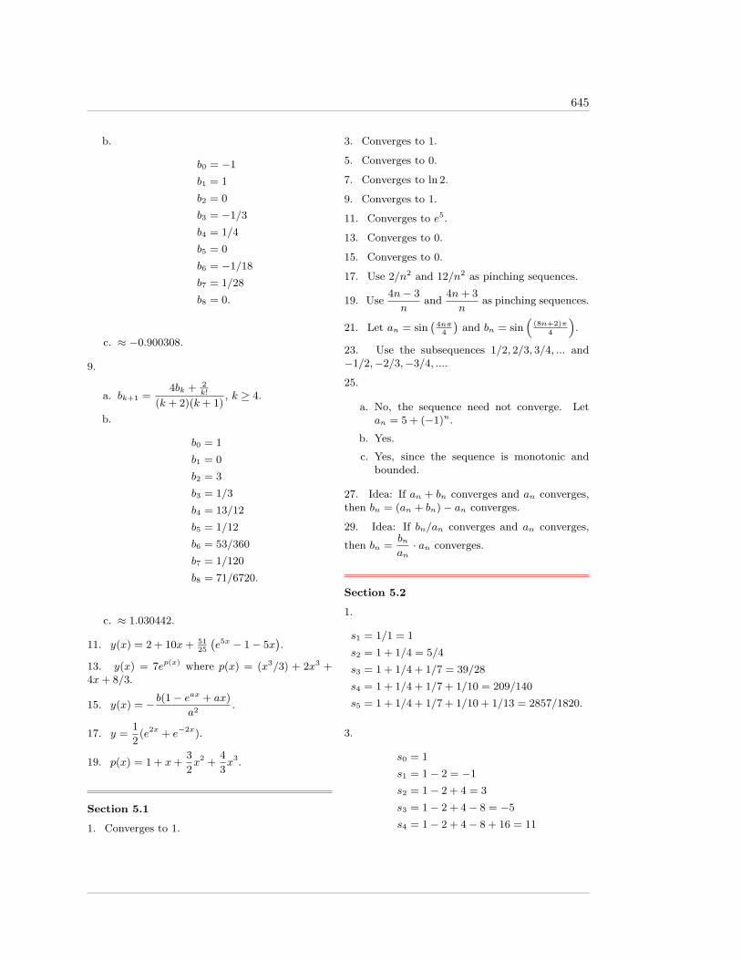
645
b.
b0 = −1
b1 = 1
b2 = 0
b3 = −1/3
b4 = 1/4
b5 = 0
b6 = −1/18
b7 = 1/28
b8 = 0.
c. ≈ −0.900308.
9.
a. bk+1 =4bk + 2
k!
(k + 2)(k + 1), k ≥ 4.
b.
b0 = 1
b1 = 0
b2 = 3
b3 = 1/3
b4 = 13/12
b5 = 1/12
b6 = 53/360
b7 = 1/120
b8 = 71/6720.
c. ≈ 1.030442.
11. y(x) = 2 + 10x+ 5125
`e5x − 1− 5x
´.
13. y(x) = 7ep(x) where p(x) = (x3/3) + 2x3 +4x+ 8/3.
15. y(x) = − b(1− eax + ax)
a2.
17. y =1
2(e2x + e−2x).
19. p(x) = 1 + x+3
2x2 +
4
3x3.
Section 5.1
1. Converges to 1.
3. Converges to 1.
5. Converges to 0.
7. Converges to ln 2.
9. Converges to 1.
11. Converges to e5.
13. Converges to 0.
15. Converges to 0.
17. Use 2/n2 and 12/n2 as pinching sequences.
19. Use4n− 3
nand
4n+ 3
nas pinching sequences.
21. Let an = sin`
4nπ4
´and bn = sin
“(8n+2)π
4
”.
23. Use the subsequences 1/2, 2/3, 3/4, ... and−1/2,−2/3,−3/4, ....
25.
a. No, the sequence need not converge. Letan = 5 + (−1)n.
b. Yes.
c. Yes, since the sequence is monotonic andbounded.
27. Idea: If an + bn converges and an converges,then bn = (an + bn)− an converges.
29. Idea: If bn/an converges and an converges,
then bn =bnan· an converges.
Section 5.2
1.
s1 = 1/1 = 1
s2 = 1 + 1/4 = 5/4
s3 = 1 + 1/4 + 1/7 = 39/28
s4 = 1 + 1/4 + 1/7 + 1/10 = 209/140
s5 = 1 + 1/4 + 1/7 + 1/10 + 1/13 = 2857/1820.
3.
s0 = 1
s1 = 1− 2 = −1
s2 = 1− 2 + 4 = 3
s3 = 1− 2 + 4− 8 = −5
s4 = 1− 2 + 4− 8 + 16 = 11
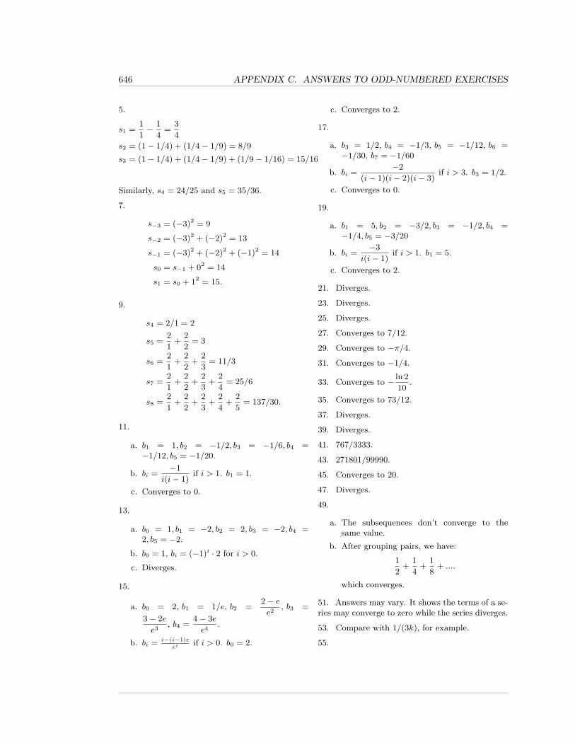
646 APPENDIX C. ANSWERS TO ODD-NUMBERED EXERCISES
5.
s1 =1
1− 1
4=
3
4
s2 = (1− 1/4) + (1/4− 1/9) = 8/9
s3 = (1− 1/4) + (1/4− 1/9) + (1/9− 1/16) = 15/16
Similarly, s4 = 24/25 and s5 = 35/36.
7.
s−3 = (−3)2 = 9
s−2 = (−3)2 + (−2)2 = 13
s−1 = (−3)2 + (−2)2 + (−1)2 = 14
s0 = s−1 + 02 = 14
s1 = s0 + 12 = 15.
9.
s4 = 2/1 = 2
s5 =2
1+
2
2= 3
s6 =2
1+
2
2+
2
3= 11/3
s7 =2
1+
2
2+
2
3+
2
4= 25/6
s8 =2
1+
2
2+
2
3+
2
4+
2
5= 137/30.
11.
a. b1 = 1, b2 = −1/2, b3 = −1/6, b4 =−1/12, b5 = −1/20.
b. bi =−1
i(i− 1)if i > 1. b1 = 1.
c. Converges to 0.
13.
a. b0 = 1, b1 = −2, b2 = 2, b3 = −2, b4 =2, b5 = −2.
b. b0 = 1, bi = (−1)i · 2 for i > 0.
c. Diverges.
15.
a. b0 = 2, b1 = 1/e, b2 =2− ee2
, b3 =
3− 2e
e3, b4 =
4− 3e
e4.
b. bi = i−(i−1)e
eiif i > 0. b0 = 2.
c. Converges to 2.
17.
a. b3 = 1/2, b4 = −1/3, b5 = −1/12, b6 =−1/30, b7 = −1/60
b. bi =−2
(i− 1)(i− 2)(i− 3)if i > 3. b3 = 1/2.
c. Converges to 0.
19.
a. b1 = 5, b2 = −3/2, b3 = −1/2, b4 =−1/4, b5 = −3/20
b. bi =−3
i(i− 1)if i > 1. b1 = 5.
c. Converges to 2.
21. Diverges.
23. Diverges.
25. Diverges.
27. Converges to 7/12.
29. Converges to −π/4.
31. Converges to −1/4.
33. Converges to − ln 2
10.
35. Converges to 73/12.
37. Diverges.
39. Diverges.
41. 767/3333.
43. 271801/99990.
45. Converges to 20.
47. Diverges.
49.
a. The subsequences don’t converge to thesame value.
b. After grouping pairs, we have:
1
2+
1
4+
1
8+ ....
which converges.
51. Answers may vary. It shows the terms of a se-ries may converge to zero while the series diverges.
53. Compare with 1/(3k), for example.
55.
647
a. 1 +
∞Xk=1
2
3k.
b. 2.
c. The dog runs twice as fast as the man, andso covers twice the distance.
Section 5.3
1. Diverges by the p-Series Test.
3.
a. Converges by the p-Series Test.
b. Using inequalities from p-Series Test, be-
tween 49 − 7“
1 + 2−8/7 + 3−8/7”
and 56 −
7“
1 + 2−8/7 + 3−8/7”
.
5. Diverges.
7.
a. Converges by the p-Series Test.
b. Between 5.5 and 13.5.
9. Diverges.
11. Compare with the convergent seriesX 2
k2.
13. Compare with the divergent seriesX p+ 1
1p.
15. Compare with the convergent seriesX 4
m2.
17. Compare with the divergent seriesX 2
k1/2.
19. Compare with the convergent seriesX 3
k1.1.
21. Diverges. Limit compare withX 1
k.
23. Diverges. Limit compare withX
(p+ 1).
25. Converges. Limit compare withX 1
m2.
27. Diverges. Limit compare withX 1
k1/6=X k1/3
k1/2.
29. Converges. Limit compare withX 1
2k=X √
4k
4k.
31. Converges.
33. Diverges.
35. Diverges.
37. Converges.
39. Converges.
41. Converges.
43. Diverges.
45. Hint: one can use an argument similar to theproof of the ratio test.
47. Apply the natural logarithm to the secondformula in Corollary 5.3.30.
Section 5.4
1. Converges absolutely.
3. Converges absolutely.
5. Diverges.
7. Diverges.
9. Converges absolutely.
11. Diverges.
13. Converges conditionally.
15. Converges absolutely.
17. Converges by Theorem 5.4.11. c0 = 1, c1 =−1/4, c2 = 23/72, c4 ≈ 0.183287, c5 = 139/2000.
19. Converges by Theorem 5.4.11. c0 = 1, c1 = 0,c2 = 0, c3 = 0, c4 = 0, c5 = 0.
21.
9999Xk=1
(−1)k−1 1√k.
23.
99Xk=1
(−1)k−1 1√k2 + 1
.
25. Converges conditionally.
27. Diverges.
29. The final step of both parts of the theoremfollow by the Cauchy criterion and the fact thatthe series an and bn converge absolutely.
31. Let an = bn = (−1)n√n+1
.
33. Unlike finite sums, infinite sums are not, ingeneral, commutative. The order in which termsare summed matters.
648 APPENDIX C. ANSWERS TO ODD-NUMBERED EXERCISES
35. Converges on [0.8, 1.2] and absolutely at bothendpoints.
37. Converges on [−1, 1] and absolutely at bothendpoints.
39. Converges on [−3, 11). Converges condition-ally at x = −3.
41. Converges on (−7 − e,−7 + e). Diverges atboth endpoints by the Term Test for Divergence.

Bibliography
[1] Feynman, R., Leighton, R., and Sands, M. The Feynman Lectures on Physics. Addison-Wesley, 1963.
[2] Massey, D. Worldwide Differential Calculus. Worldwide Center of Math., 1st edition, 2009.
[3] Rudin, W. Principles of Mathematical Analysis. International Series in Pure and AppliedMathematics. McGraw-Hill, 1953.
[4] Trench, William F. Introduction to Real Analysis. Prentice Hall, 2003.
649

650 BIBLIOGRAPHY
Index
i-th subinterval of a partition, 87p-Series Test, 580p-series, 580p-series, alternating, 606
Abel, Niels Henrik, 313, 487absolute convergence, 598absolute error, 181acceleration, 8acceleration vector, 621alternating p-series, 606alternating harmonic series, 455, 473, 488, 599alternating series, 605Alternating Series Test, 499, 605analytic continuation, real, 481analytic function, real, 462angle addition formulas, 502annulus, 300anti-derivative, 2anti-derivative on an interval, 142anti-differentiation, 1arc length, 258, 261, 268arc length function, 266Archimedes Principle, 385area between graphs, 228, 232, 241area function, cross-sectional, 294area in polar coordinates, 285area inside a circle, 149area swept out, 277, 279associativity for convergent series, 566average density, 345average value, 132
axis of revolution, 300
base of a cone, 298between, 83between, strictly, 83bijection, 575binomial expansion, 456binomial series, 455Binomial Theorem, 455, 456, 513bounded above, 537bounded below, 537bounded function, 110bounded set, 110, 537buoyancy force, 385
cardioid, 283Cauchy Criterion for Series Convergence, 596Cauchy product of series, 601Cauchy sequence, 537center of mass, 348, 350centered at a, 399centroid, 348choose, 456circular trigonometric functions, 58collision, inelastic, 379collision, totally inelastic, 379Comparison Test, 582completeness of the real numbers, 538completing the square, 41complex numbers, 57component functions, 619components of a vector, 616, 618
651

652 INDEX
conditional convergence, 455, 598cone, 298, 359Conservation of Energy, 366, 379Conservation of Mass-Energy, 366continuous, 619continuous summation, 116continuous variable, 532continuous, piecewise, 112continuous, uniformly, 203convergence of a sequence, 463convergence of a series, 464, 548convergent integral, 165convergent series, 464, 549converges, 445, 463–465, 531, 549converges absolutely, 468, 525, 596, 598converges conditionally, 596, 598CORDIC, 393curve, parametric, 276curve, rectifiable, 268curve, rectifiable, piecewise-regular, 268curve, simple regular, 260cylindrical shells, 307, 309
decreasing sequence, 539definite integral, 1, 83density, 334density, area-, 338, 340density, average, 345density, length-, 338, 339difference operator, 68differentiable, 619differentiable, infinitely, 414differentiating power series, 492Dirac delta function, 256Dirac, Paul, 256direction of a vector, 617discrete variable, 532disk, 300displacement, 83, 216, 251
distance traveled, 219, 253distance traveled function, 254divergent integral, 165diverges, 445, 463–465, 531, 549dot product, 617, 619dummy variable, 68, 109
eccentricity, 292Einstein, Albert, 366element of arc length, 253elementary function, 21, 513energy, kinetic, 368energy, potential, 370, 371equilibrium position, 374error, 400error in approximation, 181error, absolute, 181error, Taylor, 426Euler’s Formula, 57, 502Euler, Leonhard, 502evaluation notation, 139eventually, for a sequence, 539exceptional values method, 43extended real number, 467extension of a function, 159
factorial, 403Feynman, Richard, 349Fibonacci sequence, 82, 546finite difference, 72finite difference function, 556force field, conservative, 372Fourier series, 579Fourier, Jean Baptiste Joseph, 579Fundamental Theorem of Calculus, 21, 140Fundamental Theorem of Calculus, Part 1, 143,
208Fundamental Theorem of Calculus, Part 2, 145
Gabriel’s horn, 313, 326
INDEX 653
gamma distributed, 177gamma function, 175, 179geometric series, 451, 550geometric sum, 76germ of f , 528Golden ratio, 547greatest lower bound, 202, 537
harmonic sequence, 542harmonic series, 455, 473, 559, 561harmonic series, alternating, 488height of a cone, 298heliocentric coordinates, 292Hooke’s Law, 374hydrostatic pressure, 388hyperbolic cosine, 57, 503hyperbolic sine, 57, 503
improper integral, 165increasing sequence, 539indefinite integral, 1index of summation, 68induction, mathematical, 410infimum, 202, 537infinite series, 464infinitely differentiable, 414infinitesimal contribution, 116integer interval, 68integrable, 165, 170integrable, Riemann, 108integral function, 140integral on E, 170Integral Test, 577integral, convergent, 170integral, definite, 83, 108integral, divergent, 170integral, indefinite, 1, 2integrand, 4, 108integrating power series, 496
integration by parts, 16integration by substitution, 12integration by trigonometric substitution, 29,
32interior of an interval, 142interval centered at a, 467interval of convergence, 468, 613inverse hyperbolic trigonometric functions, 59iteration equation, 517
joule, 366
Kepler’s 2nd Law of Planetary Motion, 292Kepler, Johannes, 292Kirchoff’s Law, 27
Lagrange, Joseph-Louis, 426lamina, 338Laplace transform, 178Laplace, Pierre-Simon, 178least upper bound, 202, 537least upper bound property, 171, 538left Riemann sum, 90Leibniz, Gottfried Wilhelm, ix, 4length of a curve, 261, 268limacon, 290Limit Comparison Test, 583limits of integration, 108linear combination, 7linearity of anti-differentiation, 6linearity of differences, 73linearity of improper integrals, 171linearity of integration, 122, 206linearity of summation, 70linearization, 412Liouville, Joseph, 21long division of polynomials, 12lower bound, 537lower sum, 202
654 INDEX
Maclaurin polynomial, 411Maclaurin series, 414Maclaurin, Colin, 411magnitude, 615, 616, 618mass, 334, 339, 341mass midpoint, 339matching coefficients, 43mean value, 132Mean Value Theorem for Integration, 132measure zero, 112mesh, 86, 87Midpoint Approximation, 182midpoint Riemann sum, 91, 98moment, 350monotonic sequence, 539
Newton’s 2nd Law of Motion, 255, 349, 368,370, 372, 378
Newton, Sir Isaac, ix, 455non-negative series, 572
parameterization by arc length, 267parameterization with unit speed, 268parameterization, rectifiable, 268parameterization, simple regular, 260parameterized curve, 620parameterizes, 260partial fractions decomposition, 39, 50partial sum, 397, 399, 414, 445, 464, 465, 548partial sum of a series, 464, 549partition of an interval, 86, 87permutation of indices, 575piecewise-continuous, 112piecewise-simple regular curve, 265Pinching Theorem for Sequences, 535point-mass, 348polar coordinates, 281polynomial function, 395polynomial, centered, 399
position, 8, 249position function, 249position vector, 249, 620Power Rule for Integration, 4power series, 393, 414power series function, 465pressure vector, 385pressure, hydrostatic, 385product of series, 601Product Rule for the dot product, 620
radial vector, 349radius of convergence, 462, 468radius of interval, 467range of the index of summation, 68Ratio Test, 469, 586, 591, 602rational function, 39real analytic continuation, 481real analytic function, 462, 478, 509rearrangement, 600, 610rearrangement of a series, 575rectifiable, 268refinement of a partition, 88refinement of a sampled partition, 88remainder, 400remainder, Taylor, 426repeated linear factor, 47repeating decimal, 554represented by a power series, 444Riemann sum, 83, 88Riemann sum, left, 90right Riemann sum, 91Root Test, 589, 591, 603rose, 3-leaved, 286
sample point, 86, 87sampled partition, 87scalar, 279, 617, 618scalar multiplication, 617, 618
INDEX 655
Second Derivative Test, 441separation, totally inelastic, 379sequence, 92, 445, 463, 531sequence, Cauchy, 537sequence, decreasing, 539sequence, harmonic, 542sequence, increasing, 539series of constants, 548series, infinite, 464series, non-negative, 572shells, cylindrical, 307, 309shifting indices, 70sigma notation, 68Simpson’s Rule, 180, 187slug, 336solid of revolution, 300specific weight, 375speed, 219, 254, 621splitting summations, 69spring, 374spring constant, 375subsequence, 542subseries, 573subset, 88substitution in definite integrals, 151sum of a series, 464, 548summation, 68supremum, 202, 537surface of revolution, 321
tautological initial data, 9Taylor polynomial, 411Taylor series, 414Taylor series function, 445Taylor’s Theorem, 426Taylor’s Theorem with Integral Remainder, 442,
443Taylor, Brook, 411Taylor-Lagrange Theorem, 211, 427
telescoping series, 550, 556telescoping sum, 73Term Test for Divergence, 559terms of a series, 464, 548, 549Third Derivative Test, 441Trapezoidal Rule, 180, 184triangle inequality, 601trifolium, 288
unbounded, 110uniformly continuous, 203unit vector, 616–619universal gravitational constant, 348upper bound, 537upper sum, 202
variance, 157vector, 615vector addition, 617, 618vector-valued function, 619velocity, 9, 250velocity vector, 620vertex of a cone, 298volume, 295volume inside a sphere, 299
washer, 300work, 103, 366work done against, 370
zero vector, 615, 616, 618

656 INDEX

About the Author:
David B. Massey was born in Jacksonville, Florida in1959. He attended Duke University as an undergraduatemathematics major from 1977 to 1981, graduating summacum laude. He remained at Duke as a graduate student from1981 to 1986. He received his Ph.D. in mathematics in 1986for his results in the area of complex analytic singularities.
Professor Massey taught for two years at Duke as a grad-uate student, and then for two years, 1986-1988, as a VisitingAssistant Professor at the University of Notre Dame. In 1988, he was awarded a National ScienceFoundation Postdoctoral Research Fellowship, and went to conduct research on singularities atNortheastern University. In 1991, he assumed a regular faculty position in the MathematicsDepartment at Northeastern. He has remained at Northeastern University ever since, where heis now a Full Professor.
Professor Massey has won awards for his teaching, both as a graduate student and as afaculty member at Northeastern. He has published 32 research papers, and two research-levelbooks. In addition, he was a chapter author of the national award-winning book on teaching:“Dear Jonas: What can I say?, Chalk Talk: E-advice from Jonas Chalk, Legendary CollegeTeacher”, edited by D. Qualters and M. Diamond, New Forums Press, (2004).
Professor Massey founded the Worldwide Center of Mathematics, LLC, in the fall of 2008, inorder to give back to the mathematical community, by providing free or very low-cost materialsand resources for students and researchers.
657