Who Trades at the Close?

Implications for Price Discovery, Liquidity, and Disagreement∗

Vincent BogousslavskyCarroll School of Management

Boston Collegevincent.bogousslavsky@bc.edu

Dmitriy MuravyevEli Broad College of BusinessMichigan State University

muravyev@msu.edu

December 3, 2020

Abstract

We document the growing importance of the closing auction in the U.S. equity market andstudy its causes and implications. The closing auction accounts for a striking 7.5% of dailyvolume in 2018, up from 3.1% in 2010. The growth of indexing and ETFs shifts trading towardsthe close and distorts closing prices: they often deviate from closing quote midpoints, but thedeviations revert by half shortly after the close and fully overnight. As volume migrates towardsthe close, liquidity at the open deteriorates. Finally, we introduce a novel measure of investordisagreement, the ratio of auction-to-total volume, and show that higher disagreement positivelypredicts future stock returns.

Keywords: Closing auction, passive investing, price pressure, liquidity, investor disagreement

∗We greatly appreciate comments from Snehal Banerjee, Hank Bessembinder, Douglas Cumming (discussant),Terry Hendershott, Edwin Hu (discussant), Slava Fos, Marc Lipson, Charles Martineau, Michael Pagano (discussant),Neil Pearson, Jeff Pontiff, Chris Reilly, Andriy Shkilko, Paul Whelan, and Haoxiang Zhu and seminar participants atthe 7th Annual Conference on Financial Market Regulation, Boston College, Chapman University, Copenhagen Busi-ness School, European Finance Association Annual Meeting, FMA Annual Meeting, the Microstructure Exchange,and the University of Cincinnati. This paper was previously circulated under the title “Should We Use ClosingPrices? Institutional Price Pressure at the Close.” We are responsible for all errors.

1

1 Introduction

U.S. equities closing prices are determined in a special call auction held at the listing exchange a

few seconds after regular trading hours. The auction clears submitted orders to maximize executed

volume in a single trade. Auction closing prices are used to price mutual fund shares and derivatives,

report performance by institutional investors, compute margin and settlement payments as well as

asset value for exchange-traded funds (ETFs) and stock indices.1

While the introduction of closing auctions in the late 1990s and early 2000s has been studied (for

example, Pagano and Schwartz (2003)), little trading occurred at the auction during that period.

Recently, however, the auction has received a lot of attention from the financial press: numerous

stories suggest that trading volume is shifting towards the end of day and raise concerns about

this trend.2 Did closing volume indeed drastically increase? The growth of indexing and ETFs is

another recent trend. Are the trends in closing volume and ETF ownership related? Does the high

auction volume distort closing prices? Does the shift in trading towards the close worsen intraday

liquidity? What are the broader implications of trading at the close? To our knowledge, we are

the first to comprehensively examine the properties of end-of-day trading and especially the closing

auction under the “new regime” of enormous volume at the close.

We first show that the closing auction has become a major trading mechanism that is increas-

ingly important. In 2018, 15.2 billion dollars are traded in the closing auction across US stocks on

a typical day, which hypothetically makes it the fifth largest equity market in the world by trading

volume.3 Aggregate auction volume accounts for 7.48% of aggregate daily dollar volume in 2018,

up from 3.11% in 2010. In contrast, Smith (2006) shows that auction volume was only 0.49% of

daily total after Nasdaq introduced a closing auction in 2004. Volume during 3:30-to-3:55pm as a

share of total volume declined between 2010 and 2018. Thus, trading volume migrates not just to

the end of the trading day but to the last five minutes and especially the auction.

Who trades at the close? Passive institutional investors are benchmarked against closing prices

1We describe the NYSE and Nasdaq auctions in Appendix A. Appendix B lists quotes from corporate executives,market participants, and members of the U.S. congress on how important a proper closing price is. Closing prices inCRSP and other databases are generally determined in these closing auctions.

2For example, “The 30 minutes that have an outsized role in US stock trading. An increasing concentration ofvolumes from 3.30pm to 4pm is causing concern.”Financial Times, April 24, 2018; “NYSE Arca Suffers Glitch DuringClosing Auction.”Wall Street Journal, March 20, 2017.

3The 2018 World Federation of Exchanges report shows that average daily volume is $130B in the U.S., $62B inChina, $23B in Japan, $19B in India, $13B in Korea, $10B in U.K., $9B in Hong Kong, and $8B at Euronext.

2

for indices they track and thus seek to transact at the auction price to minimize tracking error.

Indeed, a survey by Greenwich Associates (2017) shows that investors trade in the closing auction

for two main reasons: execution at the official auction price and efficient price discovery. Using a

difference-in-difference approach, we show that ETF and passive ownership are major determinants

of auction volume. ETF and passive mutual fund ownership, but not active mutual ownership, are

strongly associated with auction volume. But ETF, active, and passive ownership have similar

and much weaker relation to volume right before the auction. Auction volume spikes on index

rebalancing days and end-of-month days, confirming that indexing and institutional rebalancing

contribute to trading at the close. Hedges are also rebalanced at the close. Auction volume spikes

on option expiration days because option market makers drop their stock delta-hedges at the close

after options expire. In contrast, auction volume is lower on and around earnings announcements,

major recurrent informational events, whereas pre-close volume is higher. Overall, passive and

other uninformed investors seem to be the primary users of the closing auction.4

We find that the closing price often substantially deviates from the closing quote midpoint

measured at the 4pm market close (and other pre-close benchmarks). Although the median time

between the end of regular trading and the auction is only seven seconds, closing price deviations

are much larger than typical seven-second price changes. The average (absolute) deviation is 8.1

basis points, and for 1% of stock-days the closing price deviates by more than 0.63%. An average

deviation corresponds to 6 million dollars in market capitalization and accounts for 5% of intraday

volatility. Higher auction volume, which likely corresponds to a larger order imbalance, leads to

larger auction deviations. Closing price deviations are highly correlated across stocks and thus

affect diversified portfolios.

Auction volume moves prices, but does it make them more or less efficient? Models such as

that of Admati and Pfleiderer (1988) predict that concentrated trading at specific times of the

day should lower costs and make prices more efficient. Prices can also deviate from fair values if

risk-averse liquidity providers absorb large order imbalances (Grossman and Miller (1988)). Hence,

more trading at the close may lead to uninformative prices. Price impact remains permanent after

4Investors can also trade at the close to avoid holding positions overnight, to avoid the complexity of executinglarge orders intraday, and to synchronize multi-leg trades. Although we cannot rule out that some of the tradingat the close aims to manipulate the closing price, it is unlikely to account for a significant fraction of total auctionvolume.

3

informed order flow, whereas prices fully revert after (uninformed) price pressure. Consistent with

price pressure being mostly uninformed, the closing price deviation mostly reverses overnight for

small stocks. The reversal is complete for large stocks. Even when adjusted for the half-spread,

auction deviations still entirely reverse. For comparison, the overnight reversal is five times smaller

for the last five minutes of trading despite similar price deviations. Variance ratio and weighted

price contribution tests further confirm that little price discovery occurs at the auction.5

Why are price distortions so large? First, for stocks with sufficient after-hours liquidity, we

find that one-third to one-half of the reversal occurs within the first half hour after the close.

Quick reversal is consistent with imperfect liquidity provision in the auction. Exchanges have

an effective monopoly over the closing auctions for their listed securities and charge high fees to

both sides of auction trades. High fees and execution uncertainty make it more costly for external

liquidity providers to participate in the auction. The rest of the reversal can compensate liquidity

providers for bearing overnight risk. Second, differences in auction design further shed light on

how imperfect competition can distort prices at the auction. NYSE floor brokers, and thus their

clients, have an exclusive right to submit so-called D-quote orders. These widely-used orders can

bypass most restrictions of standard market- and limit-on-close orders. Consistent with imperfect

competition, price deviations are consistently larger for NYSE than for Nasdaq auctions but are

similar pre-auction. Also, auction price deviations increase for firms that switch from the Nasdaq

to the NYSE.

We find that closing volume is growing and mostly uninformed. Does this shift of uninformed

volume to the close worsen liquidity during the rest of the day? Theory predicts that intraday

liquidity may deteriorate because traders optimally cluster their trades at times of higher liquidity;

i.e., “liquidity begets liquidity” (for example, Foster and Viswanathan (1990)). Our results are

consistent with this prediction. Turnover in the first 15 minutes of trading decreases by 22% for

S&P 500 stocks over our sample period. Liquidity worsens: effective spread increases by 10 basis

points, and depth at the best quotes declines by 63%. These large changes highlight a potential

side effect of the rise in passive investing. As investors cluster at the end of the day, liquidity may

5Price discovery linked to auction volume can occur when auction imbalance information starts being disseminatedshortly before the auction. We estimate a difference-in-difference regression that exploits the timing difference in thedissemination of auction imbalance information between the NYSE and Nasdaq. We find evidence consistent withauction imbalance information contributing to price discovery for small stocks but only weak evidence for large stocks.

4

dry up during the rest of the day. This trend is concerning as the opening period is crucial for

pricing in overnight news. Indeed, traders voice concerns about the lack of intraday liquidity.6

We next show how auction volume can help measure investor disagreement. Investors trade

for two broad reasons: they rebalance portfolios, and they disagree with each other (Harris and

Raviv (1993)). Although trading volume is regarded as the most direct manifestation of investor

disagreement, the rebalancing and disagreement components are difficult to separate. We intro-

duce a novel measure of disagreement – (minus) the ratio of closing auction volume to total daily

volume. As we show, auction volume is driven primarily by institutional rebalancing and indexing

rather than disagreement, while intraday volume is driven by both rebalancing and disagreement.

Thus, disagreement is high when intraday volume is high relative to auction volume. The disagree-

ment ratio is positively correlated with analyst and social media disagreements, but our measure

is available for all public stocks daily and relies on public data. Consistent with predictions of

disagreement theories, disagreement is persistent, is positively related to volatility and volume, and

is higher around earnings announcements. Finally, we study how disagreement affects asset prices.

Consistent with Banerjee and Kremer (2010), increased disagreement is associated with higher ex-

pected returns next week and month with little subsequent reversal. Decile portfolio sorts yield a

4.2% annualized alpha, while most other return predictors are not significant in our sample. The

predictability is robust to excluding hard-to-borrow, attention-grabbing, volatile, or illiquid stocks.

Our tests imply that the last midquote, which is available in CRSP, is more informationally

efficient than the official closing price. Replacing the CRSP price with the midquote matters for

two applications that we consider.7 First, using detailed daily data on the SPDR S&P 500 ETF

(SPY) and its constituents, we find that the average ETF mispricing decreases by 59% once we

use the closing midquotes for the ETF and its constituents. Thus, ETF mispricing in daily data

may largely be due to closing price deviations. Second, many violations of the put-call parity

disappear if the parity is computed with stock midquotes instead of closing prices because daily

option prices are as of 4pm, but the closing stock price is from the auction shortly after 4pm.

6“Stock-Market Traders Pile In at the Close”, Wall Street Journal, May 27, 2015. Also, The unusual marketvolatility at the open on August 24, 2015 illustrates the potential fragility of the opening period (SEC (2015)).

7Blume and Stambaugh (1983); Asparouhova, Bessembinder, and Kalcheva (2010, 2013) show that noise in closingprices can affect asset pricing tests. Hendershott and Menkveld (2014) highlight how shocks to the inventory ofliquidity providers cause temporary price deviations. We highlight a specific channel: how the large auction volumeintroduces noise into closing prices.

5

This price mis-synchronization and the fact that closing price deviations fully revert overnight

also explain why parity violations predict next-day stock return.8 The two put-call parity puzzles

are often interpreted as evidence that option prices contain superior information (Cremers and

Weinbaum (2010)); we suggest an alternative explanation.

This paper contributes to several literatures. Prior literature on equity auctions mostly focuses

on the introduction of closing auctions. Bacidore and Lipson (2001) find that closing auctions pro-

vide little benefits for firms that switch listing from the NYSE to the Nasdaq. In contrast, Pagano

and Schwartz (2003), Comerton-Forde, Lau, and McInish (2007), Chelley-Steeley (2008), Kandel,

Rindi, and Bosetti (2012), and Pagano, Peng, and Schwartz (2013) find that market quality mostly

improved when a closing auction is introduced on the Nasdaq and international exchanges in late

1990s early 2000s. Barclay, Hendershott, and Jones (2008) find that the consolidation of order

flow in the opening auction improves price discovery. Recently, Hu and Murphy (2020) show that

auction order imbalances disseminated by the NYSE ahead of the auction are less accurate than for

the Nasdaq, which can make the NYSE auctions less efficient. They highlight that floor brokers’

market power may come not only from exclusive access to D-quote orders but also through their

access to better order imbalance information. Wu and Jegadeesh (2020) argue that reversal strate-

gies based on market-on-close order imbalances are profitable.9 We contribute to this literature

by comprehensively examining the closing auction – the economic mechanisms for closing volume,

price deviations, and their implications – in the new regime with high volume at the close.

Our results do not imply that the closing auction is problematic. It might be the best trading

mechanism to produce reliable closing prices and accommodate closing volume. In fact, Nasdaq

introduced the closing cross following demand for more robust closing prices (Pagano et al. (2013)).

We also contribute to the literature that studies how the growth of passive investing, especially

ETFs, affects financial markets.10 We show that this growth contributes to the migration of trading

volume towards the close, which distorts closing prices and worsens liquidity at the beginning of

8Battalio and Schultz (2006) emphasize the importance of synchronizing stock and option prices. We show thatthe closing auction leads to mis-synchronized prices (a new mechanism) and relate it to future returns.

9Stoll and Whaley (1990),Madhavan and Panchapagesan (2000), Comerton-Forde and Rydge (2006), Mayhew,McCormick, and Spatt (2009), and Chakraborty, Pagano, and Schwartz (2012) study the role that specialists andinformation disclosure plays for opening and closing auctions.

10Cushing and Madhavan (2000) find that stock volatility is disproportionately higher in the last five minutes oftrading and partially attribute it to institutional trading. Ben-David, Franzoni, and Moussawi (2018) find that ETFownership is associated with increased volatility and reversal for the underlying constituents. Baltussen, van Bekkum,and Da (2019) associate a decline in index return autocorrelation across countries with increased passive investing.

6

the day. Our results provide a starting point to estimate aggregate costs of trading around the

close and infer indexing costs.

We contribute to the literature on investor disagreement by introducing a novel disagreement

measure that relies on auction volume to separate disagreement and portfolio rebalancing compo-

nents of volume. Existing studies mostly rely on measures of disagreement such as the dispersion in

analysts’ forecasts (Diether, Malloy, and Scherbina (2002)) or differences in opinions expressed on

social media (Cookson and Niessner (2020)) that are available for a limited sample. In contrast, our

measure is easy to compute for all publicly traded stocks at a daily frequency. We also contribute

to the active debate about the effect of disagreement on asset prices.

The paper is organized as follows. Section 2 describes the data. Section 3 explores auction

volume and price deviations at the close and their reversal. Section 4 studies the implications of

our findings for intraday liquidity and investor disagreement. Section 5 concludes. The appendix

shows that closing price distortions matter for ETF mispricing and put-call parity violations.

2 Data

We study common stocks listed on the NYSE and Nasdaq with a price greater than $5 and a market

capitalization greater than $100 million at the beginning of a month. Observations with a missing

CRSP return are excluded. We obtain auction price and volume data from the Trade and Quote

dataset (TAQ) over January 2010 to December 2018. Auction trades are reported with a special

condition by the NYSE and Nasdaq. The procedure to identify auction trades and the relevant

filters are detailed in Appendix C. End-of-day quote midpoint and spread are obtained from CRSP.

The results are similar if we use the end-of-day quote midpoint from TAQ. We exclude observations

with a crossed quote. Intraday returns and trading volumes are obtained from TAQ.

We compare the auction price to both the CRSP daily price and midquote and exclude obser-

vations for which the absolute difference between the CRSP price/midquote and the auction price

is greater than 10% of the price/midquote. This filter excludes 76 observations, which appear to be

data errors. We also exclude days with early closures from the sample. Our final sample contains

5,720,876 stock-day observations allocated across 1,887 NYSE-listed stocks (47.59% of all observa-

tions) and 2,946 Nasdaq-listed stocks (52.41% of all observations). Among NYSE- (Nasdaq-)listed

7

stocks, 99.18% (96.01%) of stock-day observations have a valid auction price.

In our empirical tests, we use the CRSP closing price to compute the price deviation at the

close. We use the CRSP closing price instead of the TAQ auction price because CRSP is much

more widely used. The two prices match in 98.95% of observations. The differences are small and

concentrated in 2010-2013 and part of 2014. The match rate is greater than 99.99% after 2014.

Our results are quantitatively similar if we use the TAQ auction price instead of the CRSP closing

price and robust to using only the second half of the sample (2015-2018).

We use the end-of-day midquote reported by CRSP, which matches with the 4pm midquote

from TAQ for 95.80% stock-days. Again, the differences are small and our results are quantitatively

similar whether we use the CRSP or TAQ midquote. We prefer the CRSP midquote because it

is easy to substitute for the closing price for researchers who already have access to CRSP. The

noisier the CRSP midquote is, the more it pushes us against finding an improvement when using

it instead of the closing price.

We retrieve institutional ownership data from the 13F filings reported in the Thomson Reuters

database and compute active and passive mutual fund ownership. A mutual fund is classified as

passive if the R2 of a regression of the fund’s holdings-implied returns on the Fama-French three

factors is greater than 95%.11 ETF ownership is obtained from the CRSP mutual fund database

for 2010 and 2011, and from ETF Global from 2012 to 2018. Option and ETF data used in two

applications are described further in the corresponding sections.

3 Volume and price deviations at the close

We first study the properties of closing auction volume and closing price. Our results suggest

that auction volume is significantly less informative than pre-close and intraday volumes. Auction

volume is strongly associated with proxies for uninformed trading. Price deviations in the auction

reverse quickly and almost entirely.

11We thank Jiacui Li for sharing data on fund activeness.

8

3.1 Auction volume

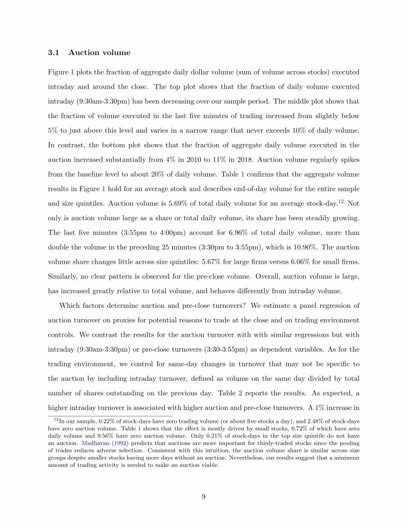
Figure 1 plots the fraction of aggregate daily dollar volume (sum of volume across stocks) executed

intraday and around the close. The top plot shows that the fraction of daily volume executed

intraday (9:30am-3:30pm) has been decreasing over our sample period. The middle plot shows that

the fraction of volume executed in the last five minutes of trading increased from slightly below

5% to just above this level and varies in a narrow range that never exceeds 10% of daily volume.

In contrast, the bottom plot shows that the fraction of aggregate daily volume executed in the

auction increased substantially from 4% in 2010 to 11% in 2018. Auction volume regularly spikes

from the baseline level to about 20% of daily volume. Table 1 confirms that the aggregate volume

results in Figure 1 hold for an average stock and describes end-of-day volume for the entire sample

and size quintiles. Auction volume is 5.69% of total daily volume for an average stock-day.12 Not

only is auction volume large as a share or total daily volume, its share has been steadily growing.

The last five minutes (3:55pm to 4:00pm) account for 6.96% of total daily volume, more than

double the volume in the preceding 25 minutes (3:30pm to 3:55pm), which is 10.90%. The auction

volume share changes little across size quintiles: 5.67% for large firms versus 6.06% for small firms.

Similarly, no clear pattern is observed for the pre-close volume. Overall, auction volume is large,

has increased greatly relative to total volume, and behaves differently from intraday volume.

Which factors determine auction and pre-close turnovers? We estimate a panel regression of

auction turnover on proxies for potential reasons to trade at the close and on trading environment

controls. We contrast the results for the auction turnover with with similar regressions but with

intraday (9:30am-3:30pm) or pre-close turnovers (3:30-3:55pm) as dependent variables. As for the

trading environment, we control for same-day changes in turnover that may not be specific to

the auction by including intraday turnover, defined as volume on the same day divided by total

number of shares outstanding on the previous day. Table 2 reports the results. As expected, a

higher intraday turnover is associated with higher auction and pre-close turnovers. A 1% increase in

12In our sample, 0.22% of stock-days have zero trading volume (or about five stocks a day), and 2.48% of stock-dayshave zero auction volume. Table 1 shows that the effect is mostly driven by small stocks, 0.72% of which have zerodaily volume and 9.56% have zero auction volume. Only 0.21% of stock-days in the top size quintile do not havean auction. Madhavan (1992) predicts that auctions are more important for thinly-traded stocks since the poolingof trades reduces adverse selection. Consistent with this intuition, the auction volume share is similar across sizegroups despite smaller stocks having more days without an auction. Nevertheless, our results suggest that a minimumamount of trading activity is needed to make an auction viable.

9

intraday turnover is associated with a 0.33% increase in auction turnover. We control for volatility

(the average absolute return over the past five days including the current day), lagged return, market

capitalization, and month-of-the-year and day-of-the-week seasonalities. Linear and quadratic trend

variables are measured in years and imply that auction turnover has been increasing by about

11.6% per year, pre-close volume turnover has a trend of 6.4% per year, and intraday turnover

stays unchanged. Stock fixed effects control for time-invariant stock-specific factors. To facilitate

interpretation, we use the logarithm of each variable except for the lagged return, trend variables,

and indicator variables. We also estimated these regressions including the lag of the dependent

variable with similar results.

Why do investors trade at the close? Passive investors strive to minimize tracking error by

trading at the auction because closing auction prices often set their benchmarks. We proxy for

indexing by ETF and passive mutual fund ownership and contrast them with active mutual fund

ownership. We control for market capitalization to distinguish the effect of institutional ownership

from size. Russell index rebalancing days (Friday in late June) provide further insights on how

passive investors trade as approximately $9 trillion in assets under management are benchmarked to

the Russell U.S. Indices. Other variables that proxy for institutional rebalancing include indicators

for beginning- and end- of-the-month, last day of the quarter, option expiration (typically third

Friday of each month). We contrast them with indicators for the day before, the day of, and the

day after an earnings announcement that proxy for periods with high informed trading.

We find that investors extensively use the closing auction for stocks with high ETF ownership.

ETF ownership is highly significant for auction turnover, but its effect on pre-close turnover is

only half as large (see Table 2). Similarly, passive mutual fund ownership is strongly associated

with auction turnover but only marginally so with pre-close and intraday turnover: a coefficient

of 0.037 versus 0.006 and 0.010. In contrast, active mutual fund ownership is positively associated

with intraday and pre-close turnover even after controlling for size, but it does not affect auction

turnover, if anything the point estimate is negative. These results are consistent with auction

volume being primarily uninformed.

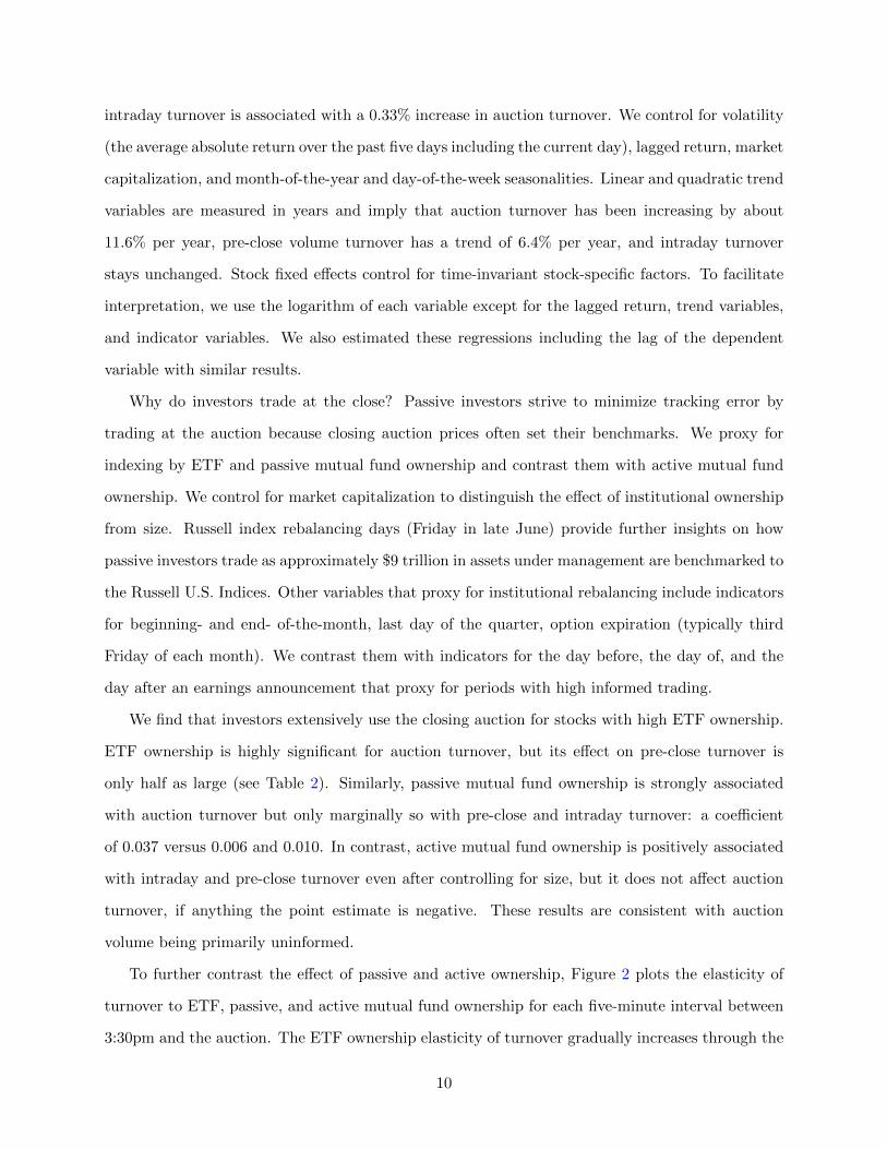
To further contrast the effect of passive and active ownership, Figure 2 plots the elasticity of

turnover to ETF, passive, and active mutual fund ownership for each five-minute interval between

3:30pm and the auction. The ETF ownership elasticity of turnover gradually increases through the

10

end of trading and spikes at the close. It is five times greater for auction turnover than for turnover

between 3:30pm and 3:35pm. The pattern for passive ownership is even more remarkable: the

volume elasticity remains roughly flat and close to zero before spiking in the auction. In contrast,

active mutual fund ownership elasticity increases gradually but drops at the auction. These results

have a difference-in-difference interpretation; the first difference compares the auction with the

pre-close; the second difference compares ETF and passive ownership with active ownership.

More formally, we estimate a two-step difference-in-difference specification. In the first step,

turnover elasticity relative to active mutual fund, passive mutual fund, and ETF ownership is es-

timated for each stock over the sample period. The elasticity is estimated separately for auction

turnover and turnover in every five-minute interval from 3:30pm until 4pm with the same set of

control variables as in Table 2. In the second step, the elasticities are regressed on indicators for

time-of-day, ownership type, and interactions between time-of-day and ownership type. Table 3 re-

ports the results. In the first column, the coefficient Auction*ETF measures the difference between

the turnover elasticities of ETF ownership and active mutual fund ownership in the auction rela-

tive to their difference in the five-minute intervals from 3:30pm to 4pm. Consistent with Figure 2,

we find that ETF and passive mutual fund elasticities are significantly larger than active mutual

fund ownership in the auction relative to the intervals before. This holds true when we only com-

pare 3:55-4:00pm with the auction, or when we focus separately on small and large stocks. This

difference-in-difference analysis helps alleviate some of the endogeneity concerns and alternative

explanations of the impact of passive ownership on closing volume.13

Since ETFs do not trade once a day at their NAVs, the benchmarking motive is not as obvious

as for passive mutual funds. Several strategies can, however, contribute to the strong link between

ETF ownership and auction turnover. First, leveraged ETFs must rebalance daily at the close to

maintain their leverage ratio. Though they often use derivatives, their counterparties hedge with

the underlying securities (Cheng and Madhavan (2009)). Second, ETFs are often traded to hedge

market risk intraday, and these hedges are closed at the end of the day. The arbitrage activity then

translates to extra volume in the underlying stocks. Finally, some ETF arbitrageurs may use the

13We also estimate an extension of the panel regression in Table 2 in which we regress auction and pre-auctionturnover on interval-stock fixed effects, and control variables and their interactions with auction/pre-auction indi-cators. This specification maps directly to the coefficients in Figure 2 except that we can formally test for thedifference-in-difference. The results are similar.

11

closing auction to complete arbitrage trades that were initiated earlier during the day.

Russell index rebalancing days provide a quasi-exogenous shock to indexing that let us confirm

its effect on closing turnover. Auction and pre-close (3:55-4:00) turnovers are 230% and 78%

higher, whereas intraday (3:30-3:55) turnover is only 7.8% higher on index rebalancing days. Index

funds rebalance in the last five minutes of trading and especially at the auction, because they

want to minimize the tracking error. Other calendar effects confirm that institutional rebalancing

contributes to closing volume. Auction and pre-close turnovers are 87% and 33% higher on the

last day of the month, while intraday turnover is unchanged. Institutional investors report their

portfolio and are benchmarked with month-end prices, which encourages them to trade at the close

to minimize tracking error. Etula et al. (2020) show that many institutional investors accommodate

inflows in the first days of the month. Indeed, turnover tends to be higher in all periods on the

first day of the month but especially so at the auction. Auction turnover is 60% higher on option

expiration days, while pre-close and intraday turnovers increase mildly (12% and 16%). Option

market-makers and other option investors, who hedge their positions in the underlying, unwind the

delta-hedge right after options expire at the close. Auction turnover is between 5% and 10% higher

in months marking a quarter-end, but there is no significant increase in auction turnover on the last

day of the quarter beyond the last day of the month increase. These results can further alleviate

endogeneity concerns as these calendar indicators are largely exogenous to the trading process.

Auction volume appears uninformed and liquidity-driven around earnings announcements. It

is well-known that informed trading is more likely around these announcements. Indeed, intraday

turnover is 22% higher on pre-announcement day, the last day before the market learns about the

news. Controlling for intraday turnover, pre-close turnover is 23% higher. In contrast, auction

turnover is virtually unchanged, a mere 1.6% increase beyond what would be predicted by higher

intraday turnover. Similarly, intraday turnover is 96% and 49% higher on the announcement and

post-announcement days, while auction turnover is about 2% lower.

Overall, auction volume appears special relative to volume at other times of the day. Auction

volume is strongly associated with proxies of uninformed and liquidity-driven trading unlike pre-

close and intraday volumes. Passive investors (index rebalancing days), other institutional investors

(month-ends), option market-makers (expiration days) extensively use the closing auction, while

informed investors (earnings announcements) do not appear to, or at least not in a substantial

12

way. Supporting this view, auction turnover depends differently on active and passive mutual

fund ownership. Why informed investors do not migrate to the auction if it is mostly composed

of uninformed volume, as predicted by models such as Admati and Pfleiderer (1988) and Collin-

Dufresne and Fos (2016)? First, the amount of uninformed trading at the close could be large

enough to dwarf informed trading. Second, trading at the close is risky because of price and

execution uncertainty on top of higher exchange fees, which we discuss further below. Ultimately,

more informed trading should lead to improved price discovery, which we investigate next.

3.2 Price deviations at the close

To study how prices deviate at the close, we define the absolute percentage deviation as

deviation% = | log(pauc/p4:00)|, (1)

where pauc is the auction price and p4:00 is the quote midpoint at 4pm.

Table 4 Panel (a) reports the distribution of closing price deviations for the entire sample and

across size quintiles. Auction price deviations are 8.12 bps on average and range from 20.6 bps

for small stocks to 2.66 bps for large stocks. To put these numbers into perspective, 8.12 bps

corresponds to 5% of daily volatility and 6 million dollars in market capitalization for an average

stock. The distribution has positive skewness: the closing price is usually close to the midquote but

occasionally deviates by a sizable amount. In 5%, 1%, and 0.1% of stock-days closing prices deviate

by more than 0.26%, 0.63%, and 1.95%, respectively. That is, prices for about 30 stocks deviate

by more than 0.63% on a typical day.14 In dollar terms, the numbers in Table 4 are economically

large given the large volume traded in the auction.

Auction price deviations contribute to daily volatility. To estimate the auction’s contribution,

we consider the volatility ratio, defined as the 20-day average of absolute deviation at the auction

divided by the 20-day average of absolute midquote return between 9:45am and 3:45pm. Table 4

Panel (b) reports the distribution for this ratio. The jump from midquote to auction price that

occurs in a few seconds (the median time between close and auction is seven seconds) accounts for

14Price deviations are also large for alternative benchmarks such as VWAP between 3:55 and 4:00pm instead of4pm midquote. We also study price deviations for large ETFs (SPY, QQQ, and S&P sectors) and find that theybehave similar to large stocks with average deviation of 3.63 bps, and 99th percentile of 16.32 bps (see Section D.2).

13

5% of daily price variation and for more than 23% for the top 1% of the sample. Even for large

stocks, average and first percentile are 3% and 12% of daily volatility. The volatility ratio decreases

monotonically with size from 9% for small stocks to 3% for large stocks. We will examine two

explanations for these results below. First, the auction may improve price discovery more for less

actively-traded stocks (Madhavan (1992)). Second, transitory liquidity shocks may have a larger

impact for smaller stocks due to limited market making capacity.15

Auction trades are rarely executed at the quote midpoint. Hence, we decompose the (absolute)

deviation into spread and price impact components: |deviation| = half-spread% + price impact%.

The (realized) half-spread is defined as log(pask/p4:00) if pauc ≥ p4:00 and log(p4:00/pbid) otherwise.

Similarly, price impact is log(pauc/pask) if pauc ≥ p4:00 and log(pbid/pauc) otherwise. Price impact

can be negative if the auction price is less than half the spread away from the closing midpoint.

Table IA.1 in the Internet Appendix reports the distribution of the half-spread and price impact

components. If the auction is like a regular small trade, then the price deviation from the midquote

will only reflect half the bid-ask spread. Larger trades will walk the limit order book creating price

impact. Indeed, the average half spread is 7.56 bps, while price impact is 0.55 bps. Thus, the price

deviation equals the half spread for most auctions similar to the bid-ask bounce. For large stocks,

the half-spread and price impact are about equal: 1.47 and 1.19 bps. Nevertheless, price impact

can be much larger than the half spread, for example, when closing volume is large.

We use panel regressions to study the determinants of closing price deviations and report the

results in Table 5.16 Higher auction turnover leads to larger price deviations: 0.88 bps higher

deviation for a 1% increase in turnover, and the impact is larger for smaller stocks. Intraday

turnover is negatively related to auction deviations perhaps because auction volume has a larger

impact on low volume days due to low liquidity. As expected, when the spread or volatility are high,

price deviations are larger. Auction volume proxies for order imbalance by liquidity seekers, which

is not directly observable in TAQ. The coefficients are quantitatively close whether we examine

15Also, for stocks of above-median size, the closing price is above the midquote more often than below. For instance,for the top-size quintile, 650,633 (597,586) deviations are above (below) the midpoint with a mean of 2.88 (2.70) basispoints. Thus, positive imbalances are more frequent than negative imbalances.

16We include auction turnover (volume normalized by shares outstanding), intraday volume excluding auction,realized volatility during the last hour and the rest of the day (computed from five-minute midquote returns), bid-askspread, stock price, (all the variables listed so far are in logs) linear and quadratic trends, and NYSE listing indicator.The main specification in Panel (a) includes stock fixed effects to focus on time-series variation. Deviation and spreadvariables are winsorized at 0.05%.

14

the absolute price deviation or price impact as reported in the Internet Appendix. Finally, NYSE

auctions have much larger deviations than Nasdaq auctions. We discuss this point in detail below.

Table 5 Panel (b) focuses on cross-stock variation by including date fixed effects instead of stock

fixed effects.

Do price deviations affect diversified portfolios? Passive investors trade baskets of securities.

This simultaneous buying or selling translates into correlated order imbalances across stocks, which

may produce correlated price deviations at the auction. To compute the aggregate price deviation,

we first aggregate signed price deviations across individual stocks for each day proportional to their

capitalization and then take the absolute value. That is, the aggregate deviation will be close to

zero if half of the stocks have a positive deviation and the other half a negative one. Aggregate

price deviation is 0.93 bps on average, or about three billion dollars per day in aggregate. The

aggregate deviation is about one third of average individual deviations for large stocks (2.66 bps

in Table 4). Figure 3 shows that the time series of aggregate price deviation and the VIX index

are highly correlated. Prices are more likely to deviate at the close when aggregate risk is high.

For instance, the largest aggregate deviation was 12 bps on August 11, 2011, when the market

rebounded after S&P downgraded U.S. sovereign debt for the fist time. These results are robust to

using only the price impact component of the aggregate price deviation and thus are not driven by a

commonality in spreads. Table IA.3 in the appendix confirms that auction volume drives aggregate

closing deviation as they both spikes on the same days, such as institutional rebalancing days. In

the time series regression of aggregate deviation on calendar indicator variables, the deviation is

27% higher on the first day of a month and on option expiration days, 60% higher on month-end,

and 159% higher on Russell rebalancing days. Thus, as price deviations are highly correlated across

stocks, they matter not only for individual stocks but also at the aggregate level.

3.3 Do closing price deviations reflect information or noise?

Auction prices deviate frequently and sometimes substantially from the 4pm midquote. Do auction

prices deviate because information is incorporated through trading or do they deviate because of

price pressure? The information hypothesis predicts that the deviation should be permanent while

deviations caused by price pressure should be reversed shortly. We test this prediction with a

15

simple model that studies how log overnight return depends on log auction deviation:

log(p9:45,t+1/pauc,t) = a+ b log(pauc,t/p4:00,t) + et, (2)

where p9:45,t+1 is the midquote price on the following day at 9:45am, pauc,t is the auction price,

and and p4:00,t is the midquote price at 4:00pm. The next-day price is adjusted for share splits and

dividends. Since quotes can be noisy and unreliable over the first couple minutes of trading, we use

the midquote 15 minutes after the open. We control for the last five-minute return (from 3:55pm

to 4pm) in some specifications.

The coefficient for price reversal b should be close to zero if auction price deviations are fully

efficient and close to -1 if they are entirely due to price pressure. Table 6 shows that the coefficient

is -0.85, or 85% of the deviation is reversed by the next morning. For large and small stocks,

110% and 85% of the price deviation is reversed. The reversal coefficient approaches -1 (complete

reversal) if we control for the 3:55-4:00 price change. Thus, price deviations are mainly due to price

pressure and not new information. In contrast, only 19% of the last five-minute return is reversed

the next morning, i.e., the 4pm midquote change is mostly efficient. Similarly, the return between

the 3:55pm midquote and the volume-weighted average price (VWAP) in the last five minutes shows

only weak reversal. In Section 3.1, we show that auction volume differs from pre-close volume. This

difference translates into prices: auction price stands out relative to pre-close price.

As the auction price reflects half the spread, we check how much of the reversal is driven by a

mechanical bounce effect. We adjust the reported auction price by adding (subtracting) half the

spread for trades made below (above) the 4pm midpoint and then estimate (2) using this spread-

adjusted auction price. The reversal coefficient becomes closer to -1 after this adjustment, -0.97

and -0.98 for large and small stocks. Overall, most of the auction deviation reverses overnight and

is uncorrelated with the bid-ask bounce.

Variance ratios are another approach to evaluate price efficiency. For each stock we compute

the ratio between daily return variance from auction prices and compare it with the variance from

quote midpoints. Table IA.4 in the appendix reports descriptive statistics for the variance ratios of

daily returns. The average ratio of 1.014 is statistically significantly different from one at the 1%

level and means that the closing price adds 1.4% of non-informative variance. The average ratio

16

for large small stocks is even larger: 4.5%.

We also compute another well-known price discovery measure – the weighted price contribution

(e.g., Barclay and Hendershott (2003)). We divide the 3:30pm-9:45am period into five-minute

intervals and measure how much each interval’s return contributes to the total return over 3:30pm-

9:45am. For each day, the weighted price contribution (WPC) for interval k is defined as

WPCk =

N∑i=1

(|ri,3:30−9:45|∑Nj=1 |rj,3:30−9:45|

)(ri,k

ri,3:30−9:45

), (3)

where ri,3:30−9:45 is the (log) return of stock i from 3:30pm to 9:45am on the next day, ri,k is the

return over interval k (for instance, between 3:50 and 3:55pm), and N the number of stocks in

the sample on that day. A stock is included, if it has an auction price on a given day and a valid

midquote at 9:45am on the next day. All returns are winsorized at 0.005%. The auction represents

only one trade, but matches a large volume. As shown in Table 1, the median auction turnover

is comparable to the 3:55-4:00 turnover and exceeds turnover in other five-minute intervals. Thus,

in volume time (i.e., the contribution per volume traded), the auction should have a similar price

contribution as other intervals, and this is why we picked a five-minute time step.

Panel (a) of Figure 4 plots WPC estimates computed across stocks in the bottom and top size

quintiles. The closing auction contributes little to price discovery as its price contribution is about

ten times lower than what other periods with similar volume contribute. The results are similar

for all size categories with the auction having slightly higher WPC for smaller stocks. (Table IA.5

in the Appendix reports WPC estimates for all size quintiles and the full sample.) If we use the

auction price adjusted for the spread, the auction’s contribution of the WPC drops to zero (reported

in Table IA.5). Thus, the auction price only conveys information to the extent that it takes place

at the ask or at the bid. These alternative price discovery measures confirm that auction price

deviations contribute little to price discovery.

An uninformative auction deviation does not imply that auction volume is uninformative since

exchanges release information about order imbalance ahead of the auction (Mayhew et al. (2009)).

As the market learns about these imbalances, prices move to reflect this information. The NYSE

(Nasdaq) starts releasing imbalance information at 3:45pm (3:50pm) over most of our sample pe-

17

riod.17 If the imbalance is informative, weighted price contributions should increase at 3:45pm

(3:50pm) for NYSE (Nasdaq) stocks to reflect the increased information flow.

We perform a simple difference-in-difference regression. WPCs for every five-minute interval

between 3:30pm and 4:00pm and the auction price deviation are averaged each day separately for

NYSE and Nasdaq stocks in a given market capitalization quintile. These WPCs are regressed

on an intercept, a NYSE indicator, indicators for each interval after 3:35pm, and NYSE-interval

interaction indicators. These last indicators allow us to test for changes in WPC while controlling

for fixed differences in WPC between different five-minute intervals at the end of the day and for

fixed differences in WPC between NYSE and Nasdaq stocks. For instance, the NYSE and 3:45pm-

3:50pm interaction coefficient allows us to test whether NYSE stocks experience a change between

their 3:45-50pm WPC and their 3:30-35pm WPC in excess of the change in WPC of Nasdaq stocks

between the same intervals.

Panel (b) of Figure 4 shows that auction volume indeed contains some information. WPC

increases for NYSE stocks when the NYSE starts to disseminate imbalance information at 3:45pm,

and this increase is not explained by a concurrent increase in the WPC of Nasdaq stocks. The

opposite holds true at 3:50pm when the Nasdaq starts to disseminate imbalance information. (The

full results are reported in Table IA.6 in the Appendix.) Though auction volume is informative,

the economic magnitudes are small. First, Panel (a) of Figure 4 shows that WPCs are stable over

3:30-4:00pm for large stocks, which is inconsistent with order dissemination playing a major role

for price informativeness. Second, Panel (b) of Figure 4 suggests that a rough estimate of auction

volume price contribution is 1% (0.5%) for small (large) stocks.18 Even taking this effect into

account, auction price contribution remains less than half of the price contribution between 3:30pm

and 3:35pm. We conclude that auction volume contributes to price discovery but is less informative

than volume over other intervals, and that this contribution is quite limited for large stocks.

17For this test, we stop our sample at the end of September 2018 since Nasdaq switched its dissemination time to3:55pm in October 2018.

18One potential concern is spillover effects if market participants learn about imbalances for Nasdaq from observedimbalances for NYSE stocks. We cannot rule out this concern, but a comparison of raw NYSE and Nasdaq WPCsuggests that this channel, if it exists, is economically small.

18

3.4 Why do closing prices reverse?

Price reversal is consistent with increased market segmentation at the auction. Exchanges have an

effective monopoly over the closing auctions for their listed securities. A closing auction for Coca

Cola’s stock organized on the Nasdaq does not set the official daily closing price for Coca Cola

since it is listed on the NYSE. Price reversal is also consistent with liquidity provision ahead of the

overnight period. Risk-averse liquidity providers likely require compensation to hold inventories in

the overnight period due to its low liquidity and high price jump risk.

To disentangle among the two explanations, we examine after-hours trades. Market segmenta-

tion predicts that some reversal should start right after the auction, whereas overnight risk predicts

that the reversal should occur mostly overnight. To compute after-hour returns, we compute

volume-weighted average prices between 4:10-4:20pm, 4:20-4:30pm, and 4:30-4:40pm.19 We start

at 4:10pm to avoid guaranteed close orders and to make sure that the auction has already taken

place and estimate

rauc-τ = a+ br4:00−auc + e, (4)

where τ is 4:20pm, 4:30pm, and 4:40pm (with stock fixed effects). Because after-hours trading is

illiquid, only large stocks that traded within this period are included, or about one third of all large

stocks for the first twenty-minute window. Table 7 shows that the price reverts half-way to the

pre-close midquote in just twenty minutes after the close. If the after-close window is expanded to

forty minutes, half of large stocks trade in this window, and the reversal coefficient is still close to

one-half. We confirm that the results are not affected by the bid-ask bounce. This fast reversal

supports the segmentation hypothesis.

Segmentation at the auction can arise for several reasons. First, exchange fees are charged on

both sides of an auction trade, whereas a rebate is issued to a trader who places a liquidity-providing

order during regular trading. Second, trading in the auction is subject to more uncertainty than

during regular hours. For example, Kim and Trepanier (2019) argue that liquidity providers face

queuing uncertainty, which makes them less willing to absorb imbalances in the closing auction. A

failed execution in the auction likely entails carrying a suboptimal inventory overnight. Thus, the

19We keep only regular trades with indicators: @ TI, @ T, @FTI, @FT for Nasdaq and T, TI, FTI, FT for NYSE.

19

reward for providing liquidity should be higher during the auction than during regular trading.

We compare auction price deviations for the NYSE with the Nasdaq to further examine market

segmentation. Although the two auctions are designed similarly as explained in Appendix A, they

differ in one important way: NYSE offers a unique order type, so-called “D-Quote.” Unlike regular

market- or limit-on-close (MOC/LOC) order types, which must be submitted prior to 3:45pm

unless offsetting a regulatory imbalance, D-Quotes can be submitted or modified until 3:59:50pm,

regardless of the current imbalance. Thus, they can exacerbate auction order imbalance and lead

to larger price deviations. D-Quotes are fully electronic orders and effectively allow traders to

circumvent the standard auction rules. D-Quotes orders are officially accessible only to NYSE floor

brokers (and thus their clients) and are only included in the NYSE order imbalance dissemination

feed at 3:55pm. Hence, the NYSE closing auction arguably subjects external liquidity providers to

significantly more uncertainty than the Nasdaq closing auction.

The segmentation hypothesis predicts that price deviations should be higher on the NYSE

than on the Nasdaq. To benchmark the NYSE closing auction deviation, we estimate a panel

regression for end-of-day absolute five-minute log returns and the auction absolute price deviation.

The regression includes a NYSE indicator and control for date fixed effects, volume, volatility,

spread, and price. We focus on large stocks to avoid issues related to thin trading but find similar

results for other size groups. Figure 5 plots the coefficient and confidence interval for the NYSE

indicator. For the 3:30-35pm, 3:35-40pm, 3:40-45pm intervals, NYSE and Nasdaq deviations are

not statistically different. Thus, our specification controls well for differences across stocks. At

3:45pm, the NYSE coefficient becomes positive and significant, as the NYSE starts to disseminate

auction order imbalance. The opposite takes place at 3:50pm, when the Nasdaq starts to release the

information. At 3:55pm, there is no significant difference despite the diffusion of D-Quotes order

imbalance on the NYSE. At the auction, the NYSE indicator is strongly positive and statistically

significant. Importantly, this excess deviation does not translate to a higher price discovery for

NYSE stocks since Panel (b) of Figure 4 shows no difference in price discovery between NYSE and

Nasdaq stocks at the auction for large stocks. We find similar evidence from panel regression with

stock fixed effects, where identification come from stocks switching exchanges. For large stocks,

the excess NYSE price deviation represents more than a third of the average price deviation in

20

Table 4.20

Hu and Murphy (2020) comprehensively study the quality of auction order imbalance infor-

mation. They argue that order imbalance information is less precise on the NYSE than on the

Nasdaq because the NYSE does not include accumulated D-Quotes to compute order imbalance

until 3:55pm. They find that auction quality is substantially worse for NYSE stocks than Nasdaq

stocks, in line with our above findings.

4 Implications

In this section, we develop several implications from our findings. First, the shift of uninformed

trading towards the end of the day that we document affects liquidity at the open. Second, auction

volume stands out relative to intraday volume since our results suggest it is primarily associated

to liquidity trading. We use this property to introduce a novel measure of investor disagreement,

validate it, and study how it affects stock prices. Finally, we show how closing price distortions

matter for ETF mispricing and put-call parity violations.

4.1 Intraday liquidity

The results so far imply that liquidity is likely to worsen during the rest of the day. We show in

Section 3.1 that closing volume is associated with proxies for passive investment strategies. As

more capital flows into these strategies, uninformed trading increases at the close. A “liquidity

begets liquidity” effect pushes other traders to also shift their trades to the close.

In models such as Admati and Pfleiderer (1988) and Foster and Viswanathan (1990), discre-

tionary liquidity traders optimally cluster their trades in the same period to lower adverse selection.

Consider an economy with two periods – open and close – and the same amount of liquidity trading

in both periods. In Admati and Pfleiderer (1988), an increase in liquidity trading at the close causes

an increase in volume and liquidity at the close, whereas liquidity and volume decrease at the open.

In Foster and Viswanathan (1990), an increase in adverse selection at the open pushes discretionary

liquidity traders to delay their trades to the close, resulting in the same prediction. The first model

20The Nasdaq closing cross is fully automated whereas the NYSE auction relies on floor brokers. As expected, themedian duration between 4pm and the auction is usually higher on the NYSE than on the Nasdaq (122 seconds vs0.2 seconds). This does not explain our results: the difference in price deviation between NYSE and Nasdaq stocksis mostly unchanged when we control for the time elapsed until the auction.

21

predicts higher volatility at the close since informed traders also migrate to the close. The second

model does not predict such a change since informed traders’ short-lived information precludes

them from moving to the close.

Intraday liquidity should deteriorate as more uninformed volume migrates to the close. To test

this prediction, we focus on another key intraday period – the open – and examine volume, liquidity,

and volatility in the first 15 and 30 minutes of trading. We restrict the sample to large stocks that

are traded over the full sample to make the stocks comparable. The sample includes 333 stocks,

with 92% of the observations belonging to S&P 500 stocks. We estimate panel regression of (log)

turnover, dollar-weighted percentage effective spread, and (log) time-weighted depth on stock fixed

effects, day and month indicators, calendar year indicators, and control variables such as stock

price and market capitalization. We focus on calendar year indicators that capture the trend in

the dependent variable: turnover, spread, and depth.

Panel (a) of Figure 6 reports the change in (log) turnover at the open and at the auction

over the sample period. Auction turnover increases, but turnover at the open decreases. Unlike

Figure 1, the plots show raw turnover, not turnover as a fraction of daily volume. The effect is

large: turnover at the open declined by around 21% (≈ e−0.24 − 1) over the sample period. This

evidence is consistent with the “liquidity begets liquidity” effect. A decrease in raw turnover is

hard to explain with alternative theories.

Also consistent with our hypothesis, liquidity deteriorates at the open over the sample period,

as shown in Panel (b). Effective spread increases and (log) depth decreases significantly, an un-

ambiguous decline in liquidity at the NBBO. Effective spread increases by around 10 bps, which

is large for S&P 500 stocks in our sample. Depth at the best quotes declines by around 63%

(≈ e−1 − 1).

Does volatility change at the open? Controlling for intraday realized volatility, realized volatility

at the open tends to increase over the sample period (see Figure IA.1 in the Internet Appendix).

This result is consistent with informed traders who act on short-lived information based on overnight

news. The release of public information over the day or competition with other informed traders

prevent these traders from delaying their trades to later during the day. Overall, as uninformed

volume migrates from the open to the close, adverse selection and volatility increase at the open.

The trading decisions of investors connect liquidity at different times of the day, and thus

22

variations in liquidity over the day ought to be examined jointly. The above results support this

idea and highlight a potential side effect of the increase in passive investing: as investors cluster at

the end of the day, liquidity may dry up during the rest of the day. Indeed, stock market traders

are concerned about the lack of intraday liquidity (see Footnote 6). The decrease in liquidity at

the open may also increase market fragility at that time. This could exacerbate events such as

the August 24, 2015, flash crash at the open, where abnormal volatility led to delayed openings

for many securities (SEC (2015)). Upson and Van Ness (2017) report that spreads do not follow

a U-Shape over the trading day anymore, with a lower spread at the close. Jiang and Yao (2020)

associate this change with trends in passive investing. These papers do not examine variations in

liquidity at the open, though their results support the “liquidity begets liquidity” effect. We believe

more work is needed in this direction given the importance of establishing a proper price after the

overnight period.

4.2 Closing volume and investor disagreement

In this section, we introduce and validate a novel measure of investor disagreement and study

how it affects asset prices. Cochrane (2011) demands that “we must answer why people trade so

much.” Harris and Raviv (1993) argue that investors are heterogeneous and trade for two broad

reasons: portfolio rebalancing and disagreement. They further clarify that “disagreements can

arise either because speculators have different private information or because they simply interpret

commonly known data differently.” Thus, informed trading can be viewed as a special type of

investor disagreement even though the two concepts are usually modeled differently. Investors

can also rebalance their portfolios in response to private liquidity shocks or changes in investment

opportunities among other reasons. Investors of course do not report why they trade; and according

to Wang (1994), a “challenge is how to identify empirically the nature of heterogeneity across

investors.” We take up this challenge.

How can we separate portfolio rebalancing and disagreement? As we show, closing volume

is mainly driven by indexing and institutional rebalancing and behaves differently from intraday

volume. We rely on these results to introduce a novel measure of disagreement – (minus) a ratio

23

of closing auction volume to total daily volume.21

Disagreementi,t = −Auction volumei,tTotal volumei,t

. (5)

The disagreement ratio is high when the daily volume is high relative to the closing volume. As-

suming the closing volume is indicative about daily rebalancing while the intraday volume contains

significant disagreement-driven trading, the ratio of the two volumes is informative about investor

disagreement. For example, if disagreement and rebalancing are split 70/30 intraday and 30/70

at the close, then the ratio of auction to intraday volume is related to the ratio of rebalancing to

disagreement (assuming intraday and auction rebalancing are correlated).

We compute a weekly average of daily disagreement ratios to facilitate the comparison with

other disagreement measures that are observed at lower frequency. Thus, the unit of observation

is stock-by-week, while the paper’s other results are at the stock-by-day level.

We first validate the disagreement ratio. Theories of disagreement such as Harris and Raviv

(1993) and Kandel and Pearson (1995) predict that it should positively relate to trading volume

and price volatility. Investors agree on how to interpret information most of the time, and periods

of high disagreement are often associated with high volume and volatility. Consistent with the

theoretical prediction, the disagreement ratio has a correlation of 28% with idiosyncratic volatility

and 24% with log daily volume in Table 8. Also, the ratio predicts volatility next month (t-stat

= 3.0) controlling for last-month volatility in a panel regression with stock and week fixed effects.

Similarly, the ratio strongly predicts total daily volume for several months in the future; a t-statistic

of 30.0 for the next-week log volume that slowly decays over time. Standard errors in all the panel

regressions in this section are clustered by stock and by week unless noted otherwise.

Most theories predict that disagreement should be persistent: if investors disagree this week,

they will likely continue to disagree next week. Consistent with this prediction, the disagreement

ratio is persistent. In a panel regression with stock and week fixed effects, the current-week ratio

predicts next-week ratio with a coefficient of 0.41, which declines to 0.31 for predicting the ratio

in four weeks. The persistence is highly statistically significant and is robust to including controls.

21The minus sign is required because prior studies focus on investor disagreement rather than agreement. Weexplore two alternative definitions – a ratio of total to auction volume and a log difference between total and auctionvolume – with similar results.

24

Kandel and Pearson (1995) make another prediction: disagreement should be higher around earn-

ings announcements. The disagreement ratio is indeed consistently higher during earnings weeks

in Table 8 (Panel (b)) even after controlling for idiosyncratic volatility, market capitalization, and

week (or stock) fixed effects.

The disagreement ratio is positively correlated with popular disagreement measures including

the analyst dispersion by Diether et al. (2002) and the social media sentiment by Cookson and Niess-

ner (2020).22 Panel (b) of Table 8 goes beyond raw correlations and shows that the disagreement

ratio positively and significantly depends on concurrent analyst and social media disagreements

and idiosyncratic volatility after controlling for log market capitalization, stock price, and weekly

fixed effects in a joint panel regression (with standard errors clustered by stock and week). Thus,

we find a robust relation between the disagreement measures. The social media and analyst dis-

agreements are only available for half of the sample, and the sample size drops four-fold if both are

included, but the results remain robust for these four samples. In contrast, the disagreement ratio

is available for any listed stock at a daily frequency, including securities without analyst coverage

such as ETFs.

After validating the disagreement ratio, we study how differences of opinion affect stock prices.

We estimate a panel regression of next-week and next-month stock returns on the change in dis-

agreement, week fixed effects (to account for the commonality of stock returns), and standard

return predictors as control variables. Stock returns are computed from daily returns in CRSP

and adjusted for stock delistings as in Shumway (1997). We skip a day between predictors and

returns to avoid confounding effects as today’s closing price is an input to tomorrow’s return. The

change in disagreement is computed as the difference between its value this week and last month.

Other predictors include idiosyncratic volatility (computed from abnormal daily returns from the

Fama-FrenchCarhart four-factor model over the prior month), momentum (stock returns from six

months to one month prior to the date), monthly reversal (previous month return), log market

capitalization, CAPM beta, Amihud (2002) illiquidity measure, and a visibility indicator, which

Gervais, Kaniel, and Mingelgrin (2001) set to one (-1) if current volume is greater (lower) than 90%

(10%) over the prior 49 days. Predictors are winsorized at a 0.05% level to avoid outliers. The

22We thank Tony Cookson for providing the social media disagreement measure on his website. It is based onmessages posted on https://stocktwits.com/ between 2010 and 2018. Following Diether et al. (2002), analyst forecastdispersion in prior month is scaled by absolute mean forecast. Analyst forecasts are from the I/B/E/S database.

25

standard stock price and market capitalization filters are already applied to the auction sample.

(Table IA.7 in the Internet Appendix reports summary statistics for the main variables.) Standard

errors are clustered by stock and week to account for overlapping returns and cross-stock depen-

dencies. The main results remain robust if a Fama-MacBeth regression is estimated instead of a

panel regression or if alternative specifications are used (for example, if current-week variables such

as return and turnover are included).

The model of Banerjee and Kremer (2010) implies that increased disagreement should be asso-

ciated with higher expected returns. Disagreement shocks are persistent (similar to ARCH effects

for volatility). Higher anticipated disagreement in the future leads to more uncertainty in payoffs

today, and this increase in risk leads investors to require a higher expected return. Consistent with

this theoretical prediction, we find that increased disagreement is associated with higher expected

returns next week and month. Table 9 reports that the change in disagreement has t-statistics of

3.1 and 4.7 for predicting weekly and monthly returns. In contrast, idiosyncratic volatility is the

only other robust predictor of monthly returns; it is well-known that many anomalies became much

weaker post-2009 which coincides with our sample period. Few variables consistently predict re-

turns, we identify a new return predictor. Consistent with a risk premium explanation, we observe

no significant return reversal if we predict second month returns with the disagreement change. We

find strong return predictability for the change in disagreement but not for its level.

We supplement panel regressions with portfolio analysis. Table 10 reports returns and alphas

from the Fama-FrenchCarhart six-factor model for equally-weighted portfolios sorted on the dis-

agreement change. The return difference between the top and bottom decile portfolios is 12 bps

for weekly returns and 34 bps for monthly returns, or 4.2% annualized, with the corresponding

t-statistics of 3.3 and 4.9. The portfolio returns increase roughly monotonically across portfolios,

and the long leg produces most of the abnormal return, thus short-sale constraints are less likely

to affect this predictability. Alphas and average returns match for the top-minus-bottom portfolio,

and factor loadings for Fama-French risk adjustment are not significantly different across top and

bottom decile portfolios. Models with fewer than six factors produce similar results.

We study increased disagreement around earnings announcements (e.g., Kandel and Pearson

(1995)) with our measure to confirm its robustness and to identify the underlying mechanism.

Banerjee and Kremer (2010) suggest that earnings announcements are likely associated with large

26

jumps in disagreement that are followed by more positive returns. Consistent with this prediction,

the disagreement ratio predicts returns more strongly around earnings announcements. We set

an earnings indicator to one if an announcement is within ten days of the current date (before

or after) and then interact this indicator with the disagreement ratio change. As reported in

Table 9, the return predictability increases two-fold around earnings announcements: a coefficient

for the disagreement ratio of 0.055 (t-stat = 5.0) versus 0.023 (t-stat = 2.7) during non-earnings

period, and this difference between the two periods is statistically significant. This application also

highlights the advantage of having a high-frequency measure of disagreement, which contrasts with

analyst forecasts that are updated less frequently.

The predictability remains unaffected when we explore important subsamples as reported in

Table IA.8 in the Internet Appendix. The results are unchanged if we exclude stocks with a non-

zero visibility indicator. Gervais et al. (2001) argue that a positive volume shock can attract new

investors, who push the stock price higher (and the reverse for negative volume shocks). Our results

are robust to excluding such stocks with visibility shocks. In untabulated results, we also confirm

that the disagreement surprise remains significant after we control for the surprise in log daily

volume (the disagreement coefficient decreases slightly from 0.033 to 0.028). Thus, benchmarking

daily volume to the auction volume (as compared to its historical average) in the disagreement

ratio makes a difference. Excluding the decile of most illiquid stocks for each week has the biggest

effect on predictability; the coefficient for disagreement decreases from 0.033 to 0.025 but remains

significant with a t-statistic of 3.4. The results are robust to excluding hard-to-borrow stocks, i.e.,

10% of stocks each week with the highest utilization or borrowing fee. The remaining 90% of stocks

are easy to borrow and have a borrowing fee of less than 1% per year. Many stock anomalies are

concentrated in illiquid or hard-to-borrow stocks, but the disagreement ratio continues to predict

returns even if such stocks are excluded. Thus, this result favors the risk premium explanation

rather than market inefficiency. The predictability decreases only slightly if we exclude the decile

of most volatile stocks. The return predictability is the same in the first and second parts of our

sample (pre and post 2014). Finally, the predictability is stronger for smaller firms: the coefficient

for disagreement is 0.038 for the quintile of smallest firms versus 0.023 for the quintile of largest

firms, both are significant. This is consistent with higher disagreement for small stocks.

The auction volume helps us separate disagreement from rebalancing and thus identify investor

27

disagreement. But the pre-close volume, especially outside the last five minutes of trading, is

only weakly associated with ETF ownership and institutional rebalancing. Thus, the disagreement

ratio computed from pre-close volume should be a weaker proxy for disagreement and thus a

weaker return predictor. Indeed, if the auction volume in the disagreement ratio is replaced with

the 3:55-4:00pm or 3:30-3:55pm volumes, the disagreement change loses most of its predictive

power for future returns, even though these two periods are adjacent to the auction and have

comparable volume. The last two columns in Table 9 show that for monthly returns, the auction-

based disagreement remains unaffected by adding the pre-close “disagreements:” the 3:55-4:00pm

disagreement is barely significant, and the 3:30-3:55pm disagreement does not predict returns. The

3:55-4:00 pm or 3:30-3:55pm disagreement ratios do not predict weekly returns. Thus, consistent

with the earlier ETF sensitivity results, the closing volume is indeed special relative to the pre-close

volume and can proxy for the rebalancing component of volume.

We contribute to the debate on the relation between disagreement and future stock returns.

We find that the disagreement level is not significantly related to future returns, while the change

in disagreement positively predicts returns. Diether et al. (2002) show that the level of analyst

disagreement is negatively related to future returns. They explain the predictability by arguing

that prices reflect a more optimistic valuation if pessimistic investors are kept out of the market by

high short-sale costs (Miller (1977)). Cen, Wei, and Yang (2017) argue that the analyst forecast

dispersion measure captures not only disagreement but also other return-predictive information

contained in the normalization scalars of the measure. Indeed, we find that analyst disagreement

negatively predict returns in our sample even for the subsample of easy-to-borrow stocks. Banerjee

and Kremer (2010) measure changes in disagreement with abnormal daily turnover and find that

an increase in disagreement is followed by positive returns in the next ten days on average. They

assume that volume shocks are entirely due to disagreement, while we show that rebalancing volume

varies over time and helps separate the two components. Overall, our results are consistent with a

positive risk premium for changes in disagreement.

4.3 Do closing price deviations matter?

Closing prices frequently deviate from closing midquotes, and these deviations are fully reversed,

but does using the midquote instead of the CRSP price make a difference? We show that it does for

28

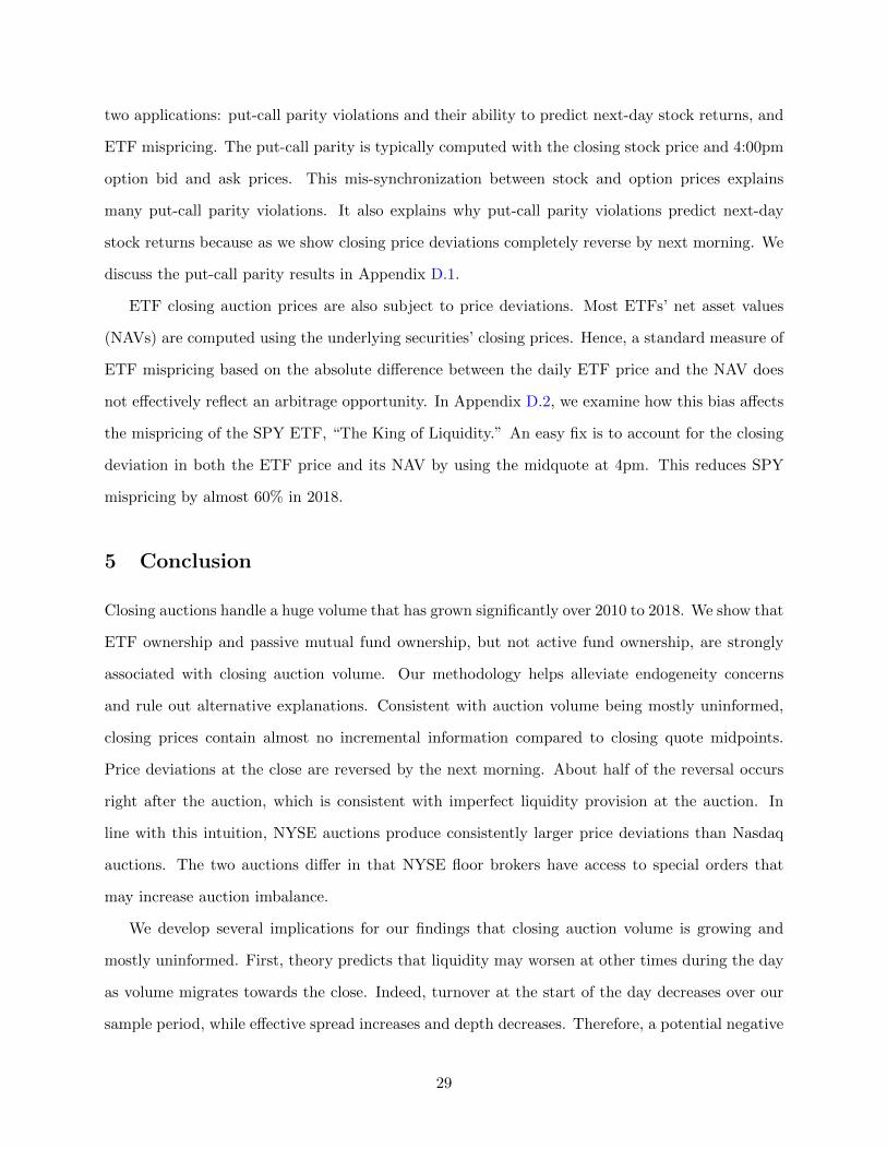
two applications: put-call parity violations and their ability to predict next-day stock returns, and

ETF mispricing. The put-call parity is typically computed with the closing stock price and 4:00pm

option bid and ask prices. This mis-synchronization between stock and option prices explains

many put-call parity violations. It also explains why put-call parity violations predict next-day

stock returns because as we show closing price deviations completely reverse by next morning. We

discuss the put-call parity results in Appendix D.1.

ETF closing auction prices are also subject to price deviations. Most ETFs’ net asset values

(NAVs) are computed using the underlying securities’ closing prices. Hence, a standard measure of

ETF mispricing based on the absolute difference between the daily ETF price and the NAV does

not effectively reflect an arbitrage opportunity. In Appendix D.2, we examine how this bias affects

the mispricing of the SPY ETF, “The King of Liquidity.” An easy fix is to account for the closing

deviation in both the ETF price and its NAV by using the midquote at 4pm. This reduces SPY

mispricing by almost 60% in 2018.

5 Conclusion

Closing auctions handle a huge volume that has grown significantly over 2010 to 2018. We show that

ETF ownership and passive mutual fund ownership, but not active fund ownership, are strongly

associated with closing auction volume. Our methodology helps alleviate endogeneity concerns

and rule out alternative explanations. Consistent with auction volume being mostly uninformed,

closing prices contain almost no incremental information compared to closing quote midpoints.

Price deviations at the close are reversed by the next morning. About half of the reversal occurs

right after the auction, which is consistent with imperfect liquidity provision at the auction. In

line with this intuition, NYSE auctions produce consistently larger price deviations than Nasdaq

auctions. The two auctions differ in that NYSE floor brokers have access to special orders that

may increase auction imbalance.

We develop several implications for our findings that closing auction volume is growing and

mostly uninformed. First, theory predicts that liquidity may worsen at other times during the day

as volume migrates towards the close. Indeed, turnover at the start of the day decreases over our

sample period, while effective spread increases and depth decreases. Therefore, a potential negative

29

externality of the rise of passive investing is that liquidity may dry up during the day. Second, we

introduce a novel measure of investor disagreement, which correlates with other disagreement mea-

sures, but is available for all public stocks daily. Future stock returns are higher after disagreement

increases. Finally, replacing the closing price with the 4pm quote midpoint, which is available in

CRSP, greatly reduces apparent ETF mispricing and the number of put-call parity violations.

Our results highlight several policy relevant issues. Auction participants pay high exchange

fees and can incur indirect costs of subsequent price reversal. Since auction deviations are highly

correlated across stocks, this suggests that institutions trading in the same direction (e.g., for

benchmarking reasons) are likely to bear this “cost of indexing” for trading in the auction. Still,

a closing call auction may be the best trading mechanism in light of existing institutional incen-

tives. The ongoing shift towards passive investing may lead to a further concentration of trading

volume around the close and make our analysis even more relevant. We leave for future research

to investigate how alternative auction designs interact with institutional benchmarks.

30

References

Admati, A. R. and P. Pfleiderer (1988). A Theory of Intraday Patterns: Volume and Price Variability.Review of Financial Studies 1 (1), 3–40.

Amihud, Y. (2002). Illiquidity and Stock Returns: Cross-Section and Time-Series Effects. Journal ofFinancial Markets 5 (1), 31–56.

Asparouhova, E., H. Bessembinder, and I. Kalcheva (2010). Liquidity biases in asset pricing tests. Journalof Financial Economics 96 (2), 215–237.

Asparouhova, E., H. Bessembinder, and I. Kalcheva (2013). Noisy Prices and Inference Regarding Returns.Journal of Finance 68 (2), 665–714.

Bacidore, J. M. and M. L. Lipson (2001). The effects of opening and closing procedures on the nyse andnasdaq. In AFA 2001 New Orleans Meetings.

Baltussen, G., S. van Bekkum, and Z. Da (2019). Indexing and stock market serial dependence around theworld. Journal of Financial Economics 132 (1), 26–48.

Banerjee, S. and I. Kremer (2010). Disagreement and learning: Dynamic patterns of trade. Journal ofFinance 65 (4), 1269–1302.

Barclay, M. J. and T. Hendershott (2003). Price discovery and trading after hours. Review of FinancialStudies 16 (4), 1041–1073.

Barclay, M. J., T. Hendershott, and C. M. Jones (2008). Order consolidation, price efficiency, and extremeliquidity shocks. Journal of Financial and Quantitative Analysis 43 (1), 93–121.

Battalio, R. and P. Schultz (2006). Options and the bubble. Journal of Finance 61 (5), 2071–2102.

Ben-David, I., F. Franzoni, and R. Moussawi (2018). Do ETFs increase volatility? Journal of Finance 73 (6),2471–2535.

Blume, L. and R. F. Stambaugh (1983). Biases in Computed Returns. Journal of Financial Economics 12 (3),387–404.

Broman, M. S. (2016). Liquidity, style investing and excess comovement of exchange-traded fund returns.Journal of Financial Markets 30, 27–53.

Cen, L., K. J. Wei, and L. Yang (2017). Disagreement, underreaction, and stock returns. ManagementScience 63 (4), 1214–1231.

Chakraborty, A., M. S. Pagano, and R. A. Schwartz (2012). Order revelation at market openings. Journalof Financial Markets 15 (2), 127–150.

Chelley-Steeley, P. L. (2008). Market quality changes in the london stock market. Journal of Banking &Finance 32 (10), 2248 – 2253.

Cheng, M. and A. Madhavan (2009). The dynamics of leveraged and inverse exchange-traded funds. Journalof Investment Management 16 (4), 43.

Cochrane, J. H. (2011). Presidential address: Discount rates. Journal of Finance 66 (4), 1047–1108.

Collin-Dufresne, P. and V. Fos (2016). Insider Trading, Stochastic Liquidity and Equilibrium Prices. Econo-metrica 84 (4), 1441–1475.

Comerton-Forde, C., S. T. Lau, and T. McInish (2007). Opening and closing behavior following the intro-duction of call auctions in singapore. Pacific-Basin Finance Journal 15 (1), 18 – 35.

Comerton-Forde, C. and J. Rydge (2006). The influence of call auction algorithm rules on market efficiency.Journal of Financial Markets 9 (2), 199–222.

Cookson, J. A. and M. Niessner (2020). Why don’t we agree? evidence from a social network of investors.Journal of Finance 75 (1), 173–228.

31

Cremers, M. and D. Weinbaum (2010). Deviations from put-call parity and stock return predictability.Journal of Financial and Quantitative Analysis 45 (2), 335–367.

Cushing, D. and A. Madhavan (2000). Stock returns and trading at the close. Journal of Financial Mar-kets 3 (1), 45–67.

Diether, K. B., C. J. Malloy, and A. Scherbina (2002). Differences of opinion and the cross section of stockreturns. Journal of Finance 57 (5), 2113–2141.

Etula, E., K. Rinne, M. Suominen, and L. Vaittinen (2020). Dash for cash: Monthly market impact ofinstitutional liquidity needs. Review of Financial Studies 33 (1), 75–111.

Foster, F. D. and S. Viswanathan (1990). A Theory of the Interday Variations in Volume, Variance, andTrading Costs in Securities Markets. Review of Financial Studies 3 (4), 593–624.

Gervais, S., R. Kaniel, and D. H. Mingelgrin (2001). The high-volume return premium. Journal of Fi-nance 56 (3), 877–919.

Goncalves-Pinto, L., B. D. Grundy, A. Hameed, T. van der Heijden, and Y. Zhu (2019). Why do optionprices predict stock returns? the role of price pressure in the stock market. FIRN Research Paper 2695145.

Grossman, S. J. and M. H. Miller (1988). Liquidity and Market Structure. Journal of Finance 43 (3),617–633.

Harris, M. and A. Raviv (1993). Differences of opinion make a horse race. Review of Financial Studies 6 (3),473–506.

Hasbrouck, J., G. Sofianos, and D. Sosebee (1993). New york stock exchange systems and trading procedures.NYSE Working Paper 93-01.

Hendershott, T. and A. J. Menkveld (2014). Price pressures. Journal of Financial Economics 114 (3),405–423.

Hu, E. and D. Murphy (2020). Vestigial tails: Floor brokers at the close in modern electronic markets.working paper.

Jiang, W. and C. Yao (2020). U disappeared: Indexing and the shift of diurnal patterns. working paper.

Kamara, A. and T. W. Miller (1995). Daily and intradaily tests of european put-call parity. Journal ofFinancial and Quantitative Analysis 30 (4), 519–539.

Kandel, E. and N. D. Pearson (1995). Differential interpretation of public signals and trade in speculativemarkets. Journal of Political Economy 103 (4), 831–872.

Kandel, E., B. Rindi, and L. Bosetti (2012). The effect of a closing call auction on market quality andtrading strategies. Journal of Financial Intermediation 21 (1), 23–49.

Kim, S. and D. Trepanier (2019). Violations of price-time priority and implications for market quality.working paper.

Klemkosky, R. C. and B. G. Resnick (1979). Put-call parity and market efficiency. Journal of Finance 34 (5),1141–1155.

Lamoureux, C. G. and J. W. Wansley (1989). The pricing of when-issued securities. Financial Review 24 (2),183–198.

Madhavan, A. (1992). Trading Mechanisms in Securities Markets. Journal of Finance 47 (2), 607–641.

Madhavan, A. and V. Panchapagesan (2000). Price discovery in auction markets: A look inside the blackbox. Review of Financial Studies 13 (3), 627–658.

Mayhew, S., T. McCormick, and C. Spatt (2009). The information content of market-on-close imbalances,the specialist and nyse equity prices. Work. Pap. 1364178.

Miller, E. M. (1977). Risk, uncertainty, and divergence of opinion. Journal of Finance 32 (4), 1151–1168.

32

Muravyev, D., N. D. Pearson, and J. M. Pollet (2018). Understanding returns to short selling using option-implied stock borrowing fees. Available at SSRN 2851560 .

Ofek, E., M. Richardson, and R. F. Whitelaw (2004). Limited arbitrage and short sales restrictions: Evidencefrom the options markets. Journal of Financial Economics 74 (2), 305–342.

Pagano, M. S., L. Peng, and R. A. Schwartz (2013). A call auction’s impact on price formation and orderrouting: Evidence from the nasdaq stock market. Journal of Financial Markets 16 (2), 331–361.

Pagano, M. S. and R. A. Schwartz (2003). A closing call’s impact on market quality at euronext paris.Journal of Financial Economics 68 (3), 439–484.

Petajisto, A. (2017). Inefficiencies in the pricing of exchange-traded funds. Financial Analysts Journal 73 (1),24–54.

Phillips, S. M. and C. W. Smith Jr (1980). Trading costs for listed options: The implications for marketefficiency. Journal of Financial Economics 8 (2), 179–201.

SEC (2015). Research Note: Equity Market Volatility on August 24, 2015. Staff of the U.S. Securities andExchange Commission.

Shumway, T. (1997). The delisting bias in crsp data. Journal of Finance 52 (1), 327–340.

Smith, J. W. (2006). Nasdaq’s electronic closing cross: An empirical analysis. Journal of Trading 1 (3),47–64.

Stoll, H. R. (1969). The relationship between put and call option prices. Journal of Finance 24 (5), 801–824.

Stoll, H. R. and R. E. Whaley (1990). Stock Market Structure and Volatility. Review of Financial Stud-ies 3 (1), 37–71.

Upson, J. and R. A. Van Ness (2017). Multiple markets, algorithmic trading, and market liquidity. Journalof Financial Markets 32, 49–68.

Wang, J. (1994). A model of competitive stock trading volume. Journal of political Economy 102 (1),127–168.

Wu, Y. and N. Jegadeesh (2020). Closing auctions: Information content and timeliness of price reaction.Working paper Emory University.

33

Figure 1. Fraction of aggregate daily dollar volume executed intraday and around the close. Dailydollar volume is summed across stocks over a given interval and then divided by the total dailydollar volume across stocks over the day. The sample consists of NYSE and Nasdaq common stocksfrom January 2010 to December 2018. To be included in a given month, a stock must have a pricegreater than $5 and a market capitalization larger than 100 million at the beginning of the month.

2010 11 12 13 14 15 16 17 180.4

0.6

0.8

Fra

ctio

nof

aggre

gate

volu

me

Intraday (9:30am-3:30pm)

2010 11 12 13 14 15 16 17 180

0.1

0.2

0.3

Fra

ctio

nof

aggre

gate

volu

me

Last five minutes (3:55pm-4:00pm)

2010 11 12 13 14 15 16 17 180

0.1

0.2

0.3

Year

Fra

ctio

nof

aggre

gate

volu

me

Auction

34

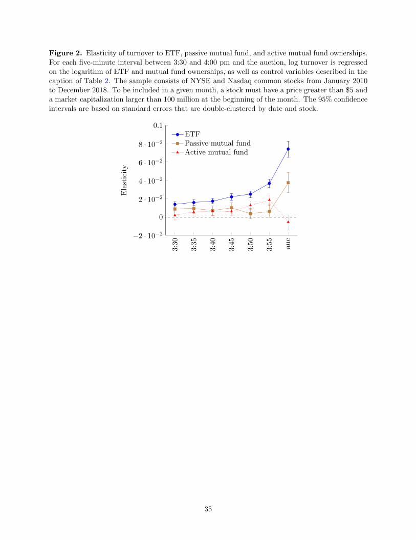
Figure 2. Elasticity of turnover to ETF, passive mutual fund, and active mutual fund ownerships.For each five-minute interval between 3:30 and 4:00 pm and the auction, log turnover is regressedon the logarithm of ETF and mutual fund ownerships, as well as control variables described in thecaption of Table 2. The sample consists of NYSE and Nasdaq common stocks from January 2010to December 2018. To be included in a given month, a stock must have a price greater than $5 anda market capitalization larger than 100 million at the beginning of the month. The 95% confidenceintervals are based on standard errors that are double-clustered by date and stock.

3:30

3:35

3:40

3:45

3:50

3:55

auc−2 · 10−2

0

2 · 10−2

4 · 10−2

6 · 10−2

8 · 10−2

0.1E

last

icit

y

ETFPassive mutual fundActive mutual fund

35

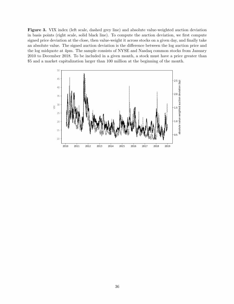
Figure 3. VIX index (left scale, dashed grey line) and absolute value-weighted auction deviationin basis points (right scale, solid black line). To compute the auction deviation, we first computesigned price deviation at the close, then value-weight it across stocks on a given day, and finally takean absolute value. The signed auction deviation is the difference between the log auction price andthe log midquote at 4pm. The sample consists of NYSE and Nasdaq common stocks from January2010 to December 2018. To be included in a given month, a stock must have a price greater than$5 and a market capitalization larger than 100 million at the beginning of the month.

36

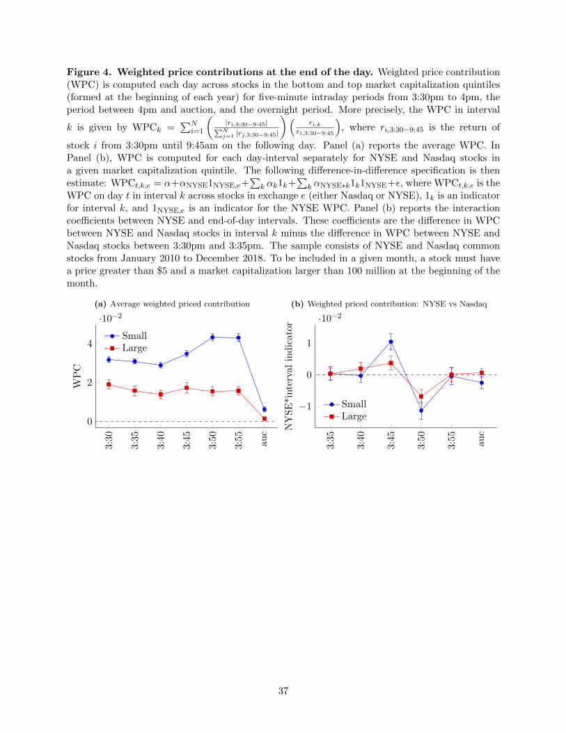
Figure 4. Weighted price contributions at the end of the day. Weighted price contribution(WPC) is computed each day across stocks in the bottom and top market capitalization quintiles(formed at the beginning of each year) for five-minute intraday periods from 3:30pm to 4pm, theperiod between 4pm and auction, and the overnight period. More precisely, the WPC in interval

k is given by WPCk =∑N

i=1

(|ri,3:30−9:45|∑Nj=1 |rj,3:30−9:45|

)(ri,k

ri,3:30−9:45

), where ri,3:30−9:45 is the return of

stock i from 3:30pm until 9:45am on the following day. Panel (a) reports the average WPC. InPanel (b), WPC is computed for each day-interval separately for NYSE and Nasdaq stocks ina given market capitalization quintile. The following difference-in-difference specification is thenestimate: WPCt,k,e = α+αNYSE1NYSE,e+

∑k αk1k+

∑k αNYSE∗k1k1NYSE+ε, where WPCt,k,e is the

WPC on day t in interval k across stocks in exchange e (either Nasdaq or NYSE), 1k is an indicatorfor interval k, and 1NYSE,e is an indicator for the NYSE WPC. Panel (b) reports the interactioncoefficients between NYSE and end-of-day intervals. These coefficients are the difference in WPCbetween NYSE and Nasdaq stocks in interval k minus the difference in WPC between NYSE andNasdaq stocks between 3:30pm and 3:35pm. The sample consists of NYSE and Nasdaq commonstocks from January 2010 to December 2018. To be included in a given month, a stock must havea price greater than $5 and a market capitalization larger than 100 million at the beginning of themonth.

(a) Average weighted priced contribution

3:30

3:35

3:40

3:45

3:50

3:55

auc

0

2

4

·10−2

WP

C

SmallLarge

(b) Weighted priced contribution: NYSE vs Nasdaq

3:35

3:40

3:45

3:50

3:55

auc

−1

0

1

·10−2

NY

SE

*inte

rval

ind

icat

or

SmallLarge

37

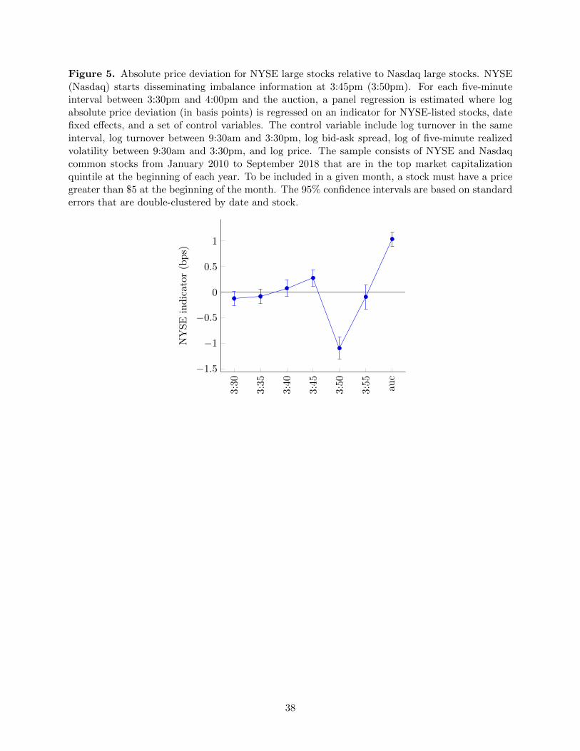
Figure 5. Absolute price deviation for NYSE large stocks relative to Nasdaq large stocks. NYSE(Nasdaq) starts disseminating imbalance information at 3:45pm (3:50pm). For each five-minuteinterval between 3:30pm and 4:00pm and the auction, a panel regression is estimated where logabsolute price deviation (in basis points) is regressed on an indicator for NYSE-listed stocks, datefixed effects, and a set of control variables. The control variable include log turnover in the sameinterval, log turnover between 9:30am and 3:30pm, log bid-ask spread, log of five-minute realizedvolatility between 9:30am and 3:30pm, and log price. The sample consists of NYSE and Nasdaqcommon stocks from January 2010 to September 2018 that are in the top market capitalizationquintile at the beginning of each year. To be included in a given month, a stock must have a pricegreater than $5 at the beginning of the month. The 95% confidence intervals are based on standarderrors that are double-clustered by date and stock.

3:30

3:35

3:40

3:45

3:50

3:55

auc

−1.5

−1

−0.5

0

0.5

1

NY

SE

ind

icat

or

(bp

s)

38

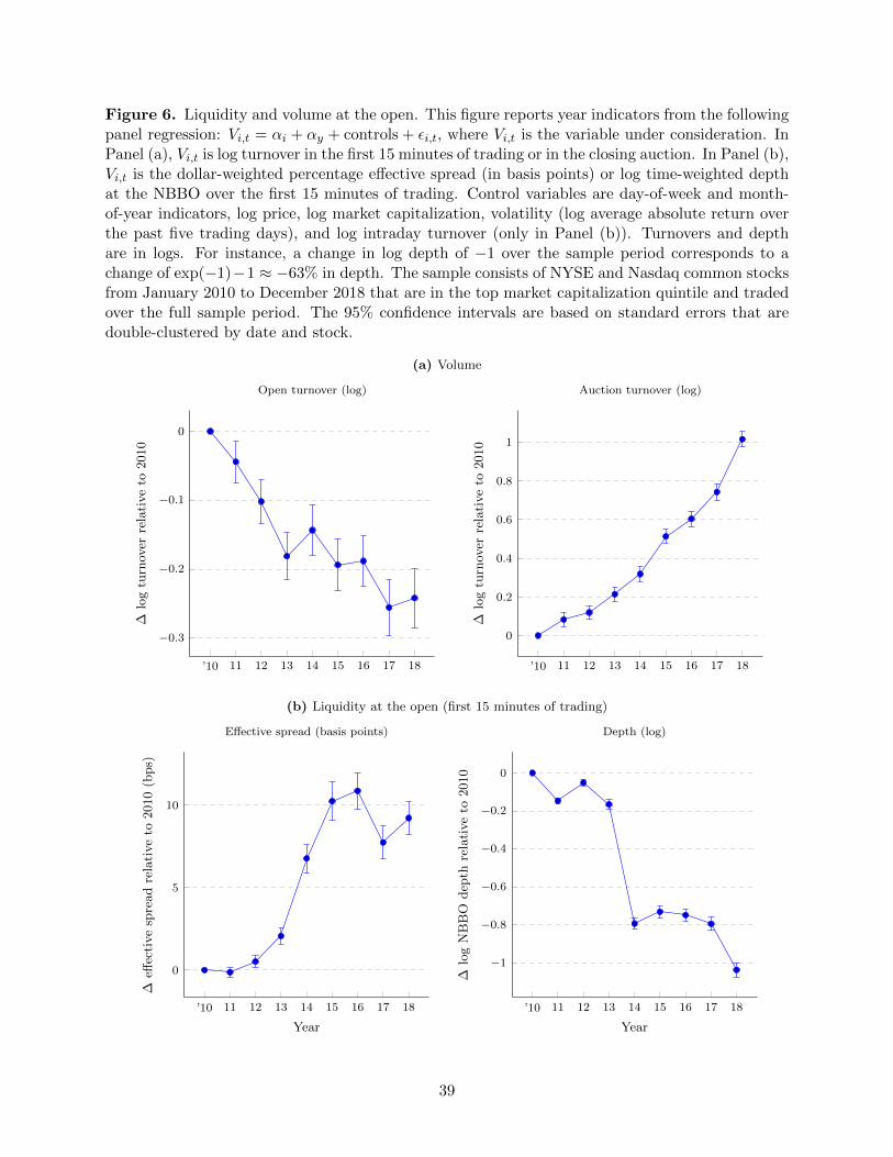
Figure 6. Liquidity and volume at the open. This figure reports year indicators from the followingpanel regression: Vi,t = αi + αy + controls + εi,t, where Vi,t is the variable under consideration. InPanel (a), Vi,t is log turnover in the first 15 minutes of trading or in the closing auction. In Panel (b),Vi,t is the dollar-weighted percentage effective spread (in basis points) or log time-weighted depthat the NBBO over the first 15 minutes of trading. Control variables are day-of-week and month-of-year indicators, log price, log market capitalization, volatility (log average absolute return overthe past five trading days), and log intraday turnover (only in Panel (b)). Turnovers and depthare in logs. For instance, a change in log depth of −1 over the sample period corresponds to achange of exp(−1)−1 ≈ −63% in depth. The sample consists of NYSE and Nasdaq common stocksfrom January 2010 to December 2018 that are in the top market capitalization quintile and tradedover the full sample period. The 95% confidence intervals are based on standard errors that aredouble-clustered by date and stock.

(a) Volume

’10 11 12 13 14 15 16 17 18

−0.3

−0.2

−0.1

0

∆lo

gtu

rnov

erre

lati

ve

to2010

Open turnover (log)

’10 11 12 13 14 15 16 17 18

0

0.2

0.4

0.6

0.8

1

∆lo

gtu

rnov

erre

lati

ve

to2010

Auction turnover (log)

(b) Liquidity at the open (first 15 minutes of trading)

’10 11 12 13 14 15 16 17 18

0

5

10

Year

∆eff

ecti

ve

spre

ad

rela

tive

to2010

(bps)

Effective spread (basis points)

’10 11 12 13 14 15 16 17 18

−1

−0.8

−0.6

−0.4

−0.2

0

Year

∆lo

gN

BB

Odep

thre

lati

ve

to2010

Depth (log)

39

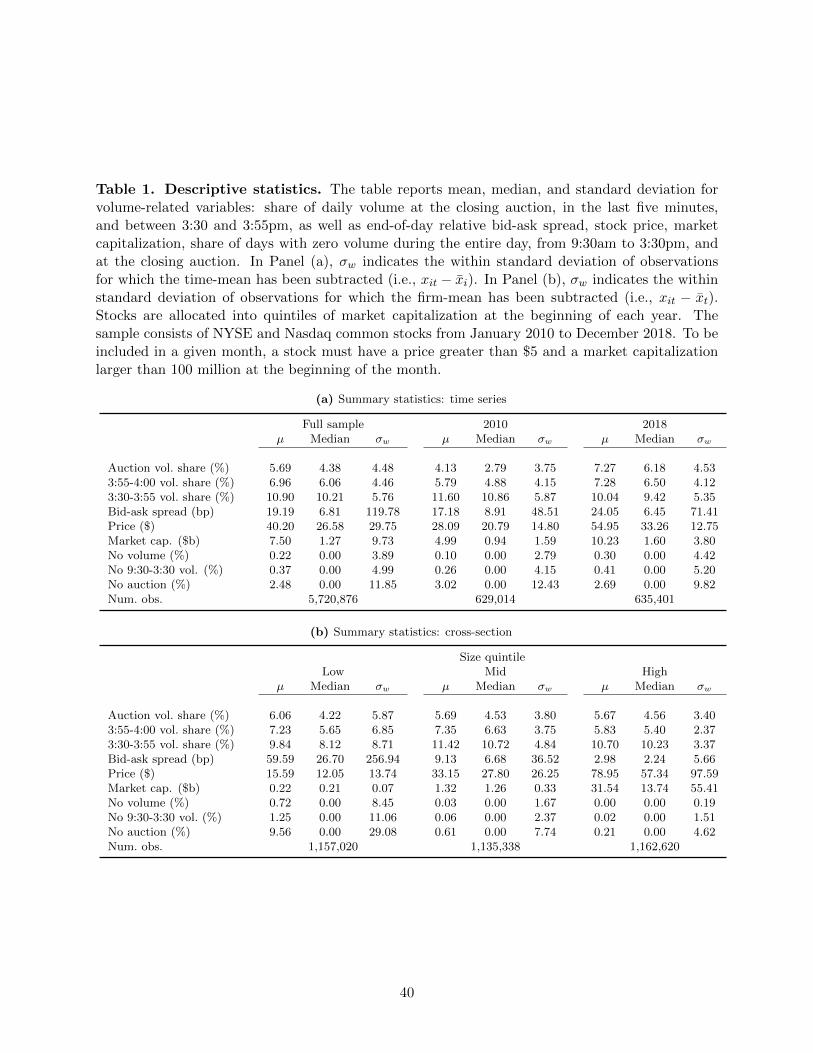
Table 1. Descriptive statistics. The table reports mean, median, and standard deviation forvolume-related variables: share of daily volume at the closing auction, in the last five minutes,and between 3:30 and 3:55pm, as well as end-of-day relative bid-ask spread, stock price, marketcapitalization, share of days with zero volume during the entire day, from 9:30am to 3:30pm, andat the closing auction. In Panel (a), σw indicates the within standard deviation of observationsfor which the time-mean has been subtracted (i.e., xit − x̄i). In Panel (b), σw indicates the withinstandard deviation of observations for which the firm-mean has been subtracted (i.e., xit − x̄t).Stocks are allocated into quintiles of market capitalization at the beginning of each year. Thesample consists of NYSE and Nasdaq common stocks from January 2010 to December 2018. To beincluded in a given month, a stock must have a price greater than $5 and a market capitalizationlarger than 100 million at the beginning of the month.

(a) Summary statistics: time series

Full sample 2010 2018µ Median σw µ Median σw µ Median σw

Auction vol. share (%) 5.69 4.38 4.48 4.13 2.79 3.75 7.27 6.18 4.533:55-4:00 vol. share (%) 6.96 6.06 4.46 5.79 4.88 4.15 7.28 6.50 4.123:30-3:55 vol. share (%) 10.90 10.21 5.76 11.60 10.86 5.87 10.04 9.42 5.35Bid-ask spread (bp) 19.19 6.81 119.78 17.18 8.91 48.51 24.05 6.45 71.41Price ($) 40.20 26.58 29.75 28.09 20.79 14.80 54.95 33.26 12.75Market cap. ($b) 7.50 1.27 9.73 4.99 0.94 1.59 10.23 1.60 3.80No volume (%) 0.22 0.00 3.89 0.10 0.00 2.79 0.30 0.00 4.42No 9:30-3:30 vol. (%) 0.37 0.00 4.99 0.26 0.00 4.15 0.41 0.00 5.20No auction (%) 2.48 0.00 11.85 3.02 0.00 12.43 2.69 0.00 9.82Num. obs. 5,720,876 629,014 635,401

(b) Summary statistics: cross-section

Size quintileLow Mid High

µ Median σw µ Median σw µ Median σw

Auction vol. share (%) 6.06 4.22 5.87 5.69 4.53 3.80 5.67 4.56 3.403:55-4:00 vol. share (%) 7.23 5.65 6.85 7.35 6.63 3.75 5.83 5.40 2.373:30-3:55 vol. share (%) 9.84 8.12 8.71 11.42 10.72 4.84 10.70 10.23 3.37Bid-ask spread (bp) 59.59 26.70 256.94 9.13 6.68 36.52 2.98 2.24 5.66Price ($) 15.59 12.05 13.74 33.15 27.80 26.25 78.95 57.34 97.59Market cap. ($b) 0.22 0.21 0.07 1.32 1.26 0.33 31.54 13.74 55.41No volume (%) 0.72 0.00 8.45 0.03 0.00 1.67 0.00 0.00 0.19No 9:30-3:30 vol. (%) 1.25 0.00 11.06 0.06 0.00 2.37 0.02 0.00 1.51No auction (%) 9.56 0.00 29.08 0.61 0.00 7.74 0.21 0.00 4.62Num. obs. 1,157,020 1,135,338 1,162,620

40

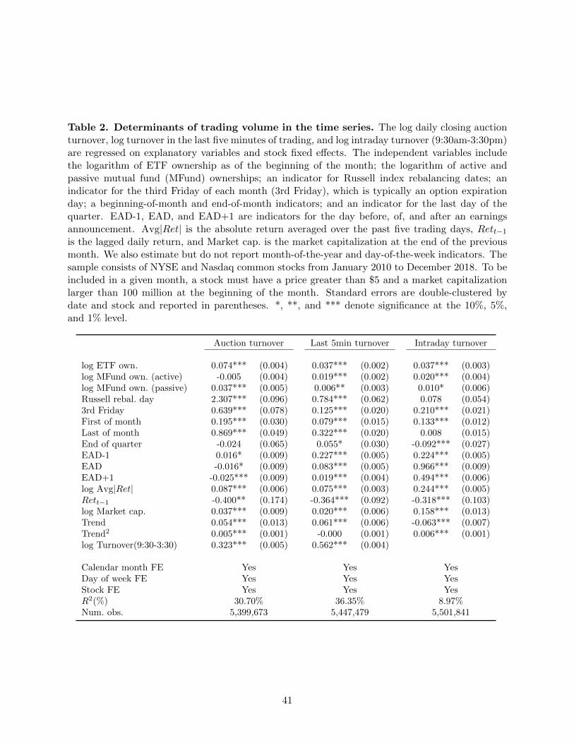
Table 2. Determinants of trading volume in the time series. The log daily closing auctionturnover, log turnover in the last five minutes of trading, and log intraday turnover (9:30am-3:30pm)are regressed on explanatory variables and stock fixed effects. The independent variables includethe logarithm of ETF ownership as of the beginning of the month; the logarithm of active andpassive mutual fund (MFund) ownerships; an indicator for Russell index rebalancing dates; anindicator for the third Friday of each month (3rd Friday), which is typically an option expirationday; a beginning-of-month and end-of-month indicators; and an indicator for the last day of thequarter. EAD-1, EAD, and EAD+1 are indicators for the day before, of, and after an earningsannouncement. Avg|Ret| is the absolute return averaged over the past five trading days, Rett−1

is the lagged daily return, and Market cap. is the market capitalization at the end of the previousmonth. We also estimate but do not report month-of-the-year and day-of-the-week indicators. Thesample consists of NYSE and Nasdaq common stocks from January 2010 to December 2018. To beincluded in a given month, a stock must have a price greater than $5 and a market capitalizationlarger than 100 million at the beginning of the month. Standard errors are double-clustered bydate and stock and reported in parentheses. *, **, and *** denote significance at the 10%, 5%,and 1% level.

Auction turnover Last 5min turnover Intraday turnover

log ETF own. 0.074*** (0.004) 0.037*** (0.002) 0.037*** (0.003)log MFund own. (active) -0.005 (0.004) 0.019*** (0.002) 0.020*** (0.004)log MFund own. (passive) 0.037*** (0.005) 0.006** (0.003) 0.010* (0.006)Russell rebal. day 2.307*** (0.096) 0.784*** (0.062) 0.078 (0.054)3rd Friday 0.639*** (0.078) 0.125*** (0.020) 0.210*** (0.021)First of month 0.195*** (0.030) 0.079*** (0.015) 0.133*** (0.012)Last of month 0.869*** (0.049) 0.322*** (0.020) 0.008 (0.015)End of quarter -0.024 (0.065) 0.055* (0.030) -0.092*** (0.027)EAD-1 0.016* (0.009) 0.227*** (0.005) 0.224*** (0.005)EAD -0.016* (0.009) 0.083*** (0.005) 0.966*** (0.009)EAD+1 -0.025*** (0.009) 0.019*** (0.004) 0.494*** (0.006)log Avg|Ret| 0.087*** (0.006) 0.075*** (0.003) 0.244*** (0.005)Rett−1 -0.400** (0.174) -0.364*** (0.092) -0.318*** (0.103)log Market cap. 0.037*** (0.009) 0.020*** (0.006) 0.158*** (0.013)Trend 0.054*** (0.013) 0.061*** (0.006) -0.063*** (0.007)Trend2 0.005*** (0.001) -0.000 (0.001) 0.006*** (0.001)log Turnover(9:30-3:30) 0.323*** (0.005) 0.562*** (0.004)

Calendar month FE Yes Yes YesDay of week FE Yes Yes YesStock FE Yes Yes YesR2(%) 30.70% 36.35% 8.97%Num. obs. 5,399,673 5,447,479 5,501,841

41

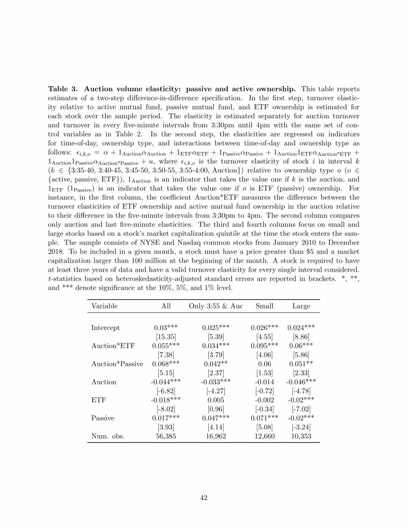
Table 3. Auction volume elasticity: passive and active ownership. This table reportsestimates of a two-step difference-in-difference specification. In the first step, turnover elastic-ity relative to active mutual fund, passive mutual fund, and ETF ownership is estimated foreach stock over the sample period. The elasticity is estimated separately for auction turnoverand turnover in every five-minute intervals from 3:30pm until 4pm with the same set of con-trol variables as in Table 2. In the second step, the elasticities are regressed on indicatorsfor time-of-day, ownership type, and interactions between time-of-day and ownership type asfollows: εi,k,o = α + 1AuctionαAuction + 1ETFαETF + 1PassiveαPassive + 1Auction1ETFαAuction*ETF +1Auction1PassiveαAuction*Passive + u, where εi,k,o is the turnover elasticity of stock i in interval k(k ∈ {3:35-40, 3:40-45, 3:45-50, 3:50-55, 3:55-4:00, Auction}) relative to ownership type o (o ∈{active, passive, ETF}), 1Auction is an indicator that takes the value one if k is the auction, and1ETF (1Passive) is an indicator that takes the value one if o is ETF (passive) ownership. Forinstance, in the first column, the coefficient Auction*ETF measures the difference between theturnover elasticities of ETF ownership and active mutual fund ownership in the auction relativeto their difference in the five-minute intervals from 3:30pm to 4pm. The second column comparesonly auction and last five-minute elasticities. The third and fourth columns focus on small andlarge stocks based on a stock’s market capitalization quintile at the time the stock enters the sam-ple. The sample consists of NYSE and Nasdaq common stocks from January 2010 to December2018. To be included in a given month, a stock must have a price greater than $5 and a marketcapitalization larger than 100 million at the beginning of the month. A stock is required to haveat least three years of data and have a valid turnover elasticity for every single interval considered.t-statistics based on heteroskedasticity-adjusted standard errors are reported in brackets. *, **,and *** denote significance at the 10%, 5%, and 1% level.

Variable All Only 3:55 & Auc Small Large

Intercept 0.03*** 0.025*** 0.026*** 0.024***[15.35] [5.39] [4.55] [8.86]

Auction*ETF 0.055*** 0.034*** 0.095*** 0.06***[7.38] [3.79] [4.06] [5.86]

Auction*Passive 0.068*** 0.042** 0.06 0.051**[5.15] [2.37] [1.53] [2.33]

Auction -0.044*** -0.033*** -0.014 -0.046***[-6.82] [-4.27] [-0.72] [-4.78]

ETF -0.018*** 0.005 -0.002 -0.02***[-8.02] [0.96] [-0.34] [-7.02]

Passive 0.017*** 0.047*** 0.071*** -0.02***[3.93] [4.14] [5.08] [-3.24]

Num. obs. 56,385 16,962 12,660 10,353

42

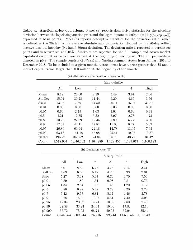
Table 4. Auction price deviations. Panel (a) reports descriptive statistics for the absolutedeviation between the log closing auction price and the log midquote at 4:00pm (= | log(pauc/p4:00)|)expressed in basis points. Panel (b) reports descriptive statistics for the deviation ratio, whichis defined as the 20-day rolling average absolute auction deviation divided by the 20-day rollingaverage absolute intraday (9:45am-3:30pm) deviation. The deviation ratio is reported in percentagepoints and is winsorized at 0.05%. Statistics are reported for the full sample and across marketcapitalization quintiles, which are formed at the beginning of each year. The xth percentile isdenoted as p0.x. The sample consists of NYSE and Nasdaq common stocks from January 2010 toDecember 2018. To be included in a given month, a stock must have a price greater than $5 and amarket capitalization larger than 100 million at the beginning of the month.

(a) Absolute auction deviation (basis points)

Size quintile

All Low 2 3 4 High

Mean 8.12 20.60 8.99 5.49 3.97 2.66StdDev 15.91 30.28 11.44 6.20 4.65 3.56Skew 13.06 7.69 14.50 20.11 16.97 33.87p0.01 0.00 0.00 0.00 0.00 0.00 0.00p0.05 0.66 2.79 1.63 1.03 0.69 0.45p0.5 4.21 12.35 6.32 3.97 2.73 1.73p0.8 10.25 27.69 12.45 7.80 5.74 3.90p0.9 17.37 42.11 17.81 11.03 8.27 5.69p0.95 26.80 60.94 24.18 14.78 11.05 7.65p0.99 63.13 141.18 45.98 25.41 19.95 13.37p0.999 195.22 356.52 124.84 56.70 43.79 31.42Count 5,578,901 1,046,362 1,104,289 1,128,456 1,139,671 1,160,123

(b) Deviation ratio (%)

Size quintile

All Low 2 3 4 High

Mean 5.01 8.68 6.25 4.75 4.14 3.41StdDev 4.69 6.60 5.12 4.26 3.93 2.81Skew 5.27 3.38 5.07 6.76 6.70 7.53p0.01 0.89 1.80 1.31 0.98 0.81 0.76p0.05 1.34 2.64 1.95 1.45 1.20 1.12p0.5 3.80 6.92 5.02 3.79 3.20 2.78p0.7 5.42 9.57 6.81 5.17 4.46 3.78p0.9 9.28 15.91 11.02 8.31 7.42 5.95p0.95 12.34 20.37 14.24 10.68 9.60 7.45p0.99 22.58 33.24 24.64 19.36 17.82 12.10p0.999 56.72 75.03 68.74 59.95 52.04 35.44Count 4,544,253 509,243 875,216 999,243 1,055,056 1,105,495

43

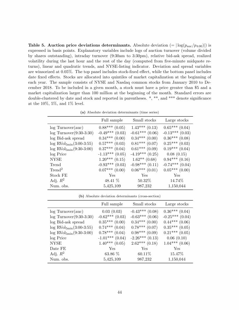
Table 5. Auction price deviations determinants. Absolute deviation (= | log(pauc/p4:00)|) isexpressed in basis points. Explanatory variables include logs of auction turnover (volume dividedby shares outstanding), intraday turnover (9:30am to 3:30pm), relative bid-ask spread, realizedvolatility during the last hour and the rest of the day (computed from five-minute midquote re-turns), linear and quadratic trends, and NYSE-listing indicator. Deviation and spread variablesare winsorized at 0.05%. The top panel includes stock-fixed effect, while the bottom panel includesdate fixed effects. Stocks are allocated into quintiles of market capitalization at the beginning ofeach year. The sample consists of NYSE and Nasdaq common stocks from January 2010 to De-cember 2018. To be included in a given month, a stock must have a price greater than $5 and amarket capitalization larger than 100 million at the beginning of the month. Standard errors aredouble-clustered by date and stock and reported in parentheses. *, **, and *** denote significanceat the 10%, 5%, and 1% level.

(a) Absolute deviation determinants (time series)

Full sample Small stocks Large stocks

log Turnover(auc) 0.88*** (0.05) 1.43*** (0.13) 0.65*** (0.04)log Turnover(9:30-3:30) -0.49*** (0.03) -0.61*** (0.06) -0.13*** (0.03)log Bid-ask spread 0.34*** (0.00) 0.34*** (0.00) 0.36*** (0.08)log RVol5min(3:00-3:55) 0.57*** (0.03) 0.81*** (0.07) 0.25*** (0.03)log RVol5min(9:30-3:00) 0.37*** (0.04) 0.61*** (0.09) 0.19*** (0.04)log Price -1.13*** (0.05) -4.19*** (0.25) 0.08 (0.15)NYSE 1.20*** (0.15) 1.62** (0.68) 0.94*** (0.16)Trend -0.93*** (0.03) -0.98*** (0.11) -0.74*** (0.04)Trend2 0.07*** (0.00) 0.06*** (0.01) 0.05*** (0.00)Stock FE Yes Yes YesAdj. R2 48.41 % 50.32% 14.74%Num. obs. 5,425,109 987,232 1,150,044

(b) Absolute deviation determinants (cross-section)

Full sample Small stocks Large stocks

log Turnover(auc) 0.03 (0.03) -0.43*** (0.08) 0.36*** (0.04)log Turnover(9:30-3:30) -0.62*** (0.03) -0.63*** (0.06) -0.25*** (0.04)log Bid-ask spread 0.35*** (0.00) 0.34*** (0.00) 0.44*** (0.06)log RVol5min(3:00-3:55) 0.74*** (0.04) 0.78*** (0.07) 0.35*** (0.05)log RVol5min(9:30-3:00) 0.78*** (0.04) 0.98*** (0.09) 0.21*** (0.05)log Price -1.01*** (0.04) -2.26*** (0.13) 0.06 (0.10)NYSE 1.40*** (0.05) 2.62*** (0.18) 1.04*** (0.06)Date FE Yes Yes YesAdj. R2 63.86 % 60.11% 15.47%Num. obs. 5,425,109 987,232 1,150,044

44

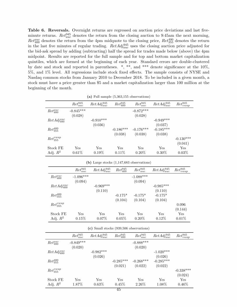
Table 6. Reversals. Overnight returns are regressed on auction price deviations and last five-minute returns. Ret945

auc denotes the return from the closing auction to 9:45am the next morning,Retauc400 denotes the return from the 4pm midquote to the closing price, Ret400

355 denotes the returnin the last five minutes of regular trading. RetAdj945

auc uses the closing auction price adjusted forthe bid-ask spread by adding (subtracting) half the spread for trades made below (above) the 4pmmidpoint. Results are reported for the full sample and for top and bottom market capitalizationquintiles, which are formed at the beginning of each year. Standard errors are double-clusteredby date and stock and reported in parentheses. *, **, and *** denote significance at the 10%,5%, and 1% level. All regressions include stock fixed effects. The sample consists of NYSE andNasdaq common stocks from January 2010 to December 2018. To be included in a given month, astock must have a price greater than $5 and a market capitalization larger than 100 million at thebeginning of the month.

(a) Full sample (5,363,155 observations)

Ret945auc RetAdj945auc Ret945400 Ret945auc RetAdj945auc Ret945vwap

Retauc400 -0.845*** -0.872***(0.028) (0.028)

RetAdjauc400 -0.910*** -0.949***(0.036) (0.037)

Ret400355 -0.186*** -0.176*** -0.185***(0.038) (0.038) (0.038)

Retvwap355 -0.130***

(0.041)Stock FE Yes Yes Yes Yes Yes YesAdj. R2 0.61% 0.19% 0.11% 0.20% 0.30% 0.03%

(b) Large stocks (1,147,683 observations)

Ret945auc RetAdj945auc Ret945400 Ret945auc RetAdj945auc Ret945vwap

Retauc400 -1.096*** -1.088***(0.094) (0.094)

RetAdjauc400 -0.969*** -0.985***(0.110) (0.110)

Ret400355 -0.175* -0.175* -0.175*(0.104) (0.104) (0.104)

Retvwap355 0.096

(0.144)Stock FE Yes Yes Yes Yes Yes YesAdj. R2 0.15% 0.07% 0.05% 0.20% 0.12% 0.01%

(c) Small stocks (939,506 observations)

Ret945auc RetAdj945auc Ret945400 Ret945auc RetAdj945auc Ret945vwap

Retauc400 -0.849*** -0.888***(0.020) (0.020)

RetAdjauc400 -0.982*** -1.020***(0.026) (0.026)

Ret400355 -0.285*** -0.268*** -0.285***(0.021) (0.022) (0.022)

Retvwap355 -0.338***

(0.024)Stock FE Yes Yes Yes Yes Yes YesAdj. R2 1.87% 0.63% 0.45% 2.26% 1.08% 0.46%

45

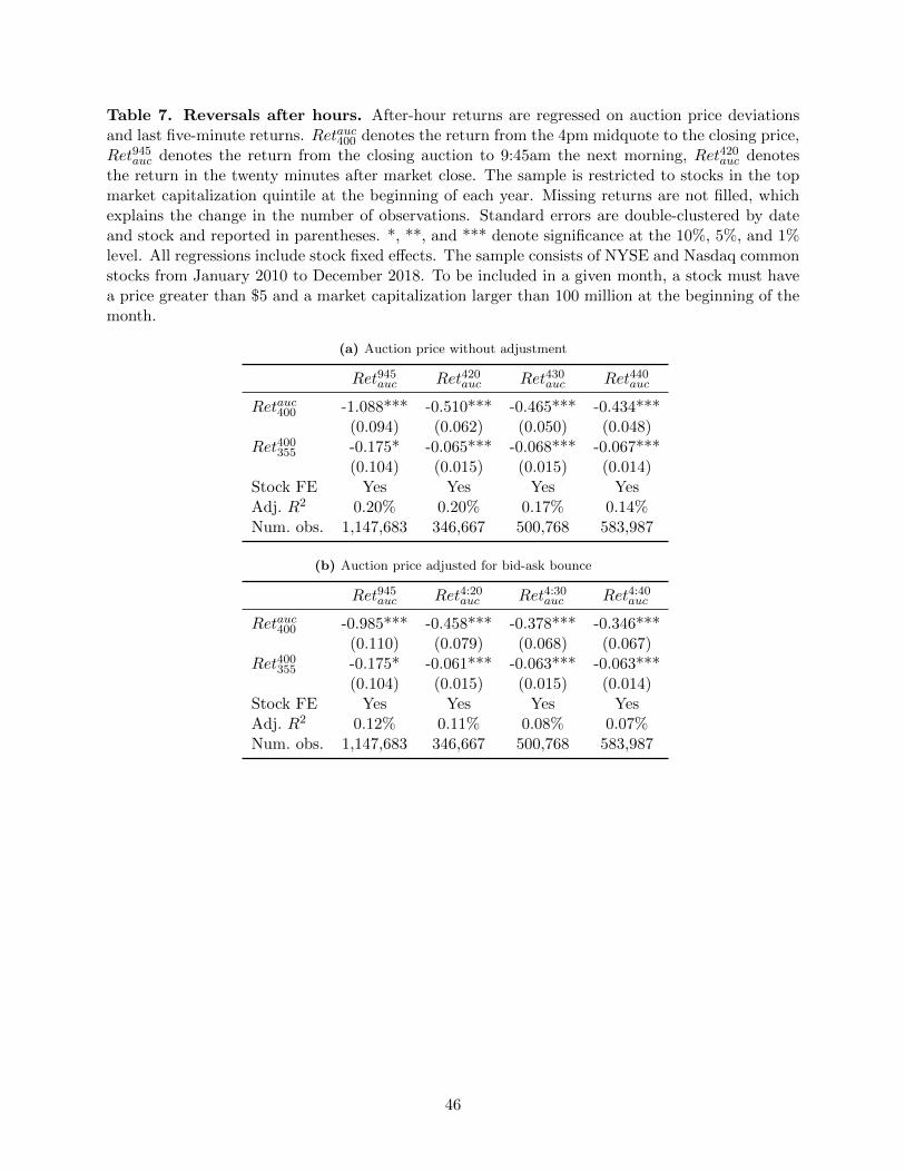
Table 7. Reversals after hours. After-hour returns are regressed on auction price deviationsand last five-minute returns. Retauc400 denotes the return from the 4pm midquote to the closing price,Ret945

auc denotes the return from the closing auction to 9:45am the next morning, Ret420auc denotes

the return in the twenty minutes after market close. The sample is restricted to stocks in the topmarket capitalization quintile at the beginning of each year. Missing returns are not filled, whichexplains the change in the number of observations. Standard errors are double-clustered by dateand stock and reported in parentheses. *, **, and *** denote significance at the 10%, 5%, and 1%level. All regressions include stock fixed effects. The sample consists of NYSE and Nasdaq commonstocks from January 2010 to December 2018. To be included in a given month, a stock must havea price greater than $5 and a market capitalization larger than 100 million at the beginning of themonth.

(a) Auction price without adjustment

Ret945auc Ret420

auc Ret430auc Ret440

auc

Retauc400 -1.088*** -0.510*** -0.465*** -0.434***(0.094) (0.062) (0.050) (0.048)

Ret400355 -0.175* -0.065*** -0.068*** -0.067***

(0.104) (0.015) (0.015) (0.014)Stock FE Yes Yes Yes YesAdj. R2 0.20% 0.20% 0.17% 0.14%Num. obs. 1,147,683 346,667 500,768 583,987

(b) Auction price adjusted for bid-ask bounce

Ret945auc Ret4:20

auc Ret4:30auc Ret4:40

auc

Retauc400 -0.985*** -0.458*** -0.378*** -0.346***(0.110) (0.079) (0.068) (0.067)

Ret400355 -0.175* -0.061*** -0.063*** -0.063***

(0.104) (0.015) (0.015) (0.014)Stock FE Yes Yes Yes YesAdj. R2 0.12% 0.11% 0.08% 0.07%Num. obs. 1,147,683 346,667 500,768 583,987

46

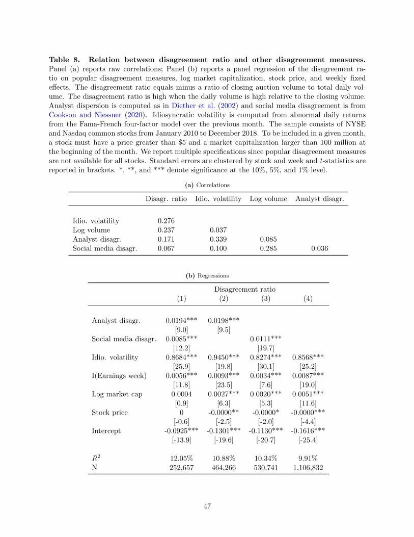
Table 8. Relation between disagreement ratio and other disagreement measures.Panel (a) reports raw correlations; Panel (b) reports a panel regression of the disagreement ra-tio on popular disagreement measures, log market capitalization, stock price, and weekly fixedeffects. The disagreement ratio equals minus a ratio of closing auction volume to total daily vol-ume. The disagreement ratio is high when the daily volume is high relative to the closing volume.Analyst dispersion is computed as in Diether et al. (2002) and social media disagreement is fromCookson and Niessner (2020). Idiosyncratic volatility is computed from abnormal daily returnsfrom the Fama-French four-factor model over the previous month. The sample consists of NYSEand Nasdaq common stocks from January 2010 to December 2018. To be included in a given month,a stock must have a price greater than $5 and a market capitalization larger than 100 million atthe beginning of the month. We report multiple specifications since popular disagreement measuresare not available for all stocks. Standard errors are clustered by stock and week and t-statistics arereported in brackets. *, **, and *** denote significance at the 10%, 5%, and 1% level.

(a) Correlations

Disagr. ratio Idio. volatility Log volume Analyst disagr.

Idio. volatility 0.276Log volume 0.237 0.037Analyst disagr. 0.171 0.339 0.085Social media disagr. 0.067 0.100 0.285 0.036

(b) Regressions

Disagreement ratio(1) (2) (3) (4)

Analyst disagr. 0.0194*** 0.0198***[9.0] [9.5]

Social media disagr. 0.0085*** 0.0111***[12.2] [19.7]

Idio. volatility 0.8684*** 0.9450*** 0.8274*** 0.8568***[25.9] [19.8] [30.1] [25.2]

I(Earnings week) 0.0056*** 0.0093*** 0.0034*** 0.0087***[11.8] [23.5] [7.6] [19.0]

Log market cap 0.0004 0.0027*** 0.0020*** 0.0051***[0.9] [6.3] [5.3] [11.6]

Stock price 0 -0.0000** -0.0000* -0.0000***[-0.6] [-2.5] [-2.0] [-4.4]

Intercept -0.0925*** -0.1301*** -0.1130*** -0.1616***[-13.9] [-19.6] [-20.7] [-25.4]

R2 12.05% 10.88% 10.34% 9.91%N 252,657 464,266 530,741 1,106,832

47

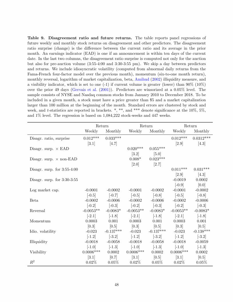
Table 9. Disagreement ratio and future returns. The table reports panel regressions offuture weekly and monthly stock returns on disagreement and other predictors. The disagreementratio surprise (change) is the difference between the current ratio and its average in the priormonth. An earnings indicator (EAD) is one if an announcement is within ten days of the currentdate. In the last two columns, the disagreement ratio surprise is computed not only for the auctionbut also for pre-auction volume (3:55-4:00 and 3:30-3:55 pm). We skip a day between predictorsand returns. We include idiosyncratic volatility (computed from abnormal daily returns from theFama-French four-factor model over the previous month), momentum (six-to-one month return),monthly reversal, logarithm of market capitalization, beta, Amihud (2002) illiquidity measure, anda visibility indicator, which is set to one (-1) if current volume is greater (lower) than 90% (10%)over the prior 49 days (Gervais et al. (2001)). Predictors are winsorized at a 0.05% level. Thesample consists of NYSE and Nasdaq common stocks from January 2010 to December 2018. To beincluded in a given month, a stock must have a price greater than $5 and a market capitalizationlarger than 100 million at the beginning of the month. Standard errors are clustered by stock andweek, and t-statistics are reported in brackets. *, **, and *** denote significance at the 10%, 5%,and 1% level. The regression is based on 1,084,222 stock-weeks and 447 weeks.

Return Return ReturnWeekly Monthly Weekly Monthly Weekly Monthly

Disagr. ratio, surprise 0.012*** 0.033*** 0.012*** 0.0312***[3.1] [4.7] [2.9] [4.3]

Disagr. surp. × EAD 0.020*** 0.055***[3.2] [5.0]

Disagr. surp. × non-EAD 0.008* 0.023***[2.0] [2.7]

Disagr. surp. for 3:55-4:00 0.011*** 0.031***[2.9] [4.3]

Disagr. surp. for 3:30-3:55 -0.0019 0.0002[-0.9] [0.0]

Log market cap. -0.0001 -0.0002 -0.0001 -0.0002 -0.0001 -0.0002[-0.5] [-0.7] [-0.5] [-0.8] [-0.5] [-0.8]

Beta -0.0002 -0.0006 -0.0002 -0.0006 -0.0002 -0.0006[-0.2] [-0.3] [-0.2] [-0.3] [-0.2] [-0.3]

Reversal -0.0053** -0.0083* -0.0053** -0.0083* -0.0053** -0.0083*[-2.1] [-1.8] [-2.1] [-1.8] [-2.1] [-1.8]

Momentum 0.0003 0.001 0.0003 0.001 0.0003 0.001[0.3] [0.5] [0.3] [0.5] [0.3] [0.5]

Idio. volatility -0.023 -0.137*** -0.023 -0.137*** -0.023 -0.138***[-1.2] [-3.2] [-1.2] [-3.2] [-1.2] [-3.2]

Illiquidity -0.0018 -0.0058 -0.0018 -0.0058 -0.0018 -0.0059[-1.0] [-1.3] [-1.0] [-1.3] [-1.0] [-1.3]

Visibility 0.0006*** 0.0002 0.0006*** 0.0002 0.0006*** 0.0002[3.1] [0.7] [3.1] [0.5] [3.1] [0.5]

R2 0.02% 0.05% 0.02% 0.05% 0.02% 0.05%

48

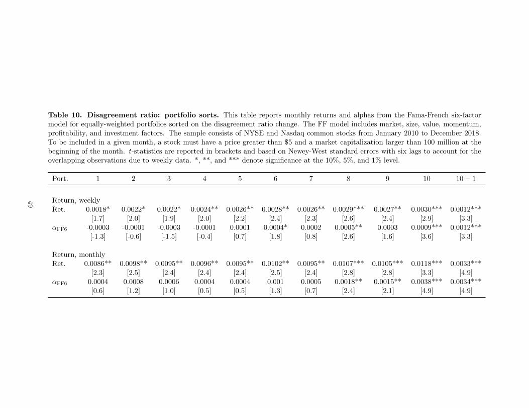
Table 10. Disagreement ratio: portfolio sorts. This table reports monthly returns and alphas from the Fama-French six-factormodel for equally-weighted portfolios sorted on the disagreement ratio change. The FF model includes market, size, value, momentum,profitability, and investment factors. The sample consists of NYSE and Nasdaq common stocks from January 2010 to December 2018.To be included in a given month, a stock must have a price greater than $5 and a market capitalization larger than 100 million at thebeginning of the month. t-statistics are reported in brackets and based on Newey-West standard errors with six lags to account for theoverlapping observations due to weekly data. *, **, and *** denote significance at the 10%, 5%, and 1% level.

Port. 1 2 3 4 5 6 7 8 9 10 10− 1

Return, weeklyRet. 0.0018* 0.0022* 0.0022* 0.0024** 0.0026** 0.0028** 0.0026** 0.0029*** 0.0027** 0.0030*** 0.0012***

[1.7] [2.0] [1.9] [2.0] [2.2] [2.4] [2.3] [2.6] [2.4] [2.9] [3.3]αFF6 -0.0003 -0.0001 -0.0003 -0.0001 0.0001 0.0004* 0.0002 0.0005** 0.0003 0.0009*** 0.0012***

[-1.3] [-0.6] [-1.5] [-0.4] [0.7] [1.8] [0.8] [2.6] [1.6] [3.6] [3.3]

Return, monthlyRet. 0.0086** 0.0098** 0.0095** 0.0096** 0.0095** 0.0102** 0.0095** 0.0107*** 0.0105*** 0.0118*** 0.0033***

[2.3] [2.5] [2.4] [2.4] [2.4] [2.5] [2.4] [2.8] [2.8] [3.3] [4.9]αFF6 0.0004 0.0008 0.0006 0.0004 0.0004 0.001 0.0005 0.0018** 0.0015** 0.0038*** 0.0034***

[0.6] [1.2] [1.0] [0.5] [0.5] [1.3] [0.7] [2.4] [2.1] [4.9] [4.9]

49

A Appendix: institutional details of closing auctions

In this section, we describe the inner workings of the closing auctions conducted by the NYSE and Nasdaq.The Nasdaq closing call auction was introduced in 2004. The NYSE also adopted a closing auction processin 2004. A matching procedure of market-on-close orders had been in effect on the NYSE since 1990 at aprice set by the prevailing ask or bid, or last trade price in case of no imbalance (Hasbrouck, Sofianos, andSosebee (1993)).

Both exchanges feature opening and closing auctions in addition to continuous trading. These are singleprice auctions where buy and sell orders are matched at a price that maximizes executed volume. Duringmost of the continuous trading session, market-on-close and limit-on-close orders can be submitted to beexecuted in the auction. After a cutoff time, such orders cannot be submitted and existing orders cannot becanceled. It is possible, however, to submit orders after the cutoff time if they are on the opposite side ofan order imbalance—meaning, if there are more sell orders than buy orders in a particular name, then it ispossible to submit a buy order after the cutoff time to help balance the book. Orders standing in the limitorder book at the end of the day also participate in the auction but with a lower priority. At the cutoff time,the exchange starts disseminating information about the auction, including the current order imbalance andthe indicative price. Figure A.1 illustrates the main features of the auction process.

Figure A.1. Conceptual trading timeline.

Open (9:30am) Close (4pm) Auction

Auction information starts being disseminatedCutoff time for market/limit on close orders

Continuous trading

Imbalance/special orders allowed

Mediantime: 7s

A.1 Nasdaq closing auction

The Nasdaq auction is simpler, so we describe it first. The Nasdaq closing cross is a call auction that crossorders at a single price. It was launched on March 29, 2004 and changed little since then, except when theclosing cross cutoff was extended from 3:50pm to 3:55pm in October 2018.

Nasdaq starts accepting market-on-close (MOC), limit-on-close (LOC) and imbalance-only (IO) ordersat 4am. A MOC order has size and direction but is entered without a price. A LOC order is executed onlyif its limit price is equal or worse than the auction price. IO orders are limit orders that provide liquidity tooffset on-close orders during the cross. An IO order to buy (or sell) is essentially converted into a limit orderat the 4pm Nasdaq best bid (ask). That is, it is re-priced to the best bid/ask on the Nasdaq book prior tothe execution of the closing cross.

Orders can be easily canceled or modified prior to 3:50pm (3:55pm since October 2018). At this time,Nasdaq stops accepting entry, cancellation, or modification of MOC orders. LOC orders received after 3:50pmare accepted only if there is a First Reference Price. Since October 2018, LOC orders may be entered until3:58pm but may not be canceled or modified. IO orders may be entered but not updated or canceled until4:00pm. Dissemination of closing information begins at 3:50pm (changed to 3:55pm in October 2018). Theclosing process begins at 4:00pm.

From 3:50pm to 4:00pm (3:55pm to 4:00pm since October 2018), Nasdaq disseminates information aboutcurrent auction order imbalance and an indicative closing price every five seconds via Nasdaq TotalViewITCH and the Nasdaq Workstation (changed to every second since October 2018). Thus, investors haveto subscribe to a special exchange data feed to observe the auction. The following information is included:current reference price within the Nasdaq Inside at which paired shares are maximized, the imbalance isminimized, and the distance from the bid-ask midpoint is minimized, in that order; near indicative clearing

50

price that will maximize the number of shares matched based on on-close orders (MOC, LOC, IO) andcontinuous market orders (effectively, this is the price at which the closing cross would occur at that momentin time); far indicative clearing price that will maximize the number of shares matched based on closinginterest only (MOC, LOC, IO), this calculation excludes continuous market orders; the number of pairedshares that can be paired off at the current reference price; imbalance quantity seeking additional liquidityat the current reference price; and imbalance side.

The closing cross occurs at 4:00pm. Nasdaq calculates the price that will maximize the number of sharesmatched based on on-close orders (MOC, LOC, IO) and continuous market orders and execute the cross ata single price called the Nasdaq Official Close Price (NOCP). Only interest on the Nasdaq book is eligibleto participate in the cross. Closing cross execution priority is as follows. MOC orders in time priority. IOorders and displayed interest of limit orders/quotes in price/time priority. Reserve size for the above executeslast at each price level before moving on to the next price level. LOC orders in price/time priority. Priorityfor IO orders will be applied after the limit prices of IO orders have been adjusted to reflect the Nasdaqinside quote at the time of the closing cross. The price is then disseminated and executions are sent to theconsolidated tape. Short selling is permitted subject to applicable short sale rules.

A.2 NYSE closing auction

The NYSE auction has the same features as the Nasdaq auction (time cutoffs and order times), but floorbrokers are given privileges adding complexity to the auction. MOC/LOC orders can be entered starting at6:30am. Imbalance information is published to Floor Broker at 2pm. The cutoff for MOC and LOC orderentry, modification, and cancellation (except for legitimate error) is 3:45pm over our sample period and waschanged to 3:50pm in January 2019. Thereafter, only offsetting MOC/LOC and closing offset (CO) ordersallowed. The cutoff for canceling a MOC/LOC for legitimate error is at 3:58pm. Cutoff for Closing D Orderentry, modification, and cancellation is at 3:59:25pm. The auction is initiated at 4pm.

The NYSE disseminates the following information: beginning at 3:45pm (changed to 3:50pm in January2019), NYSE disseminates closing auction order imbalance information; at 3:55pm, the NYSE includesClosing D Orders at their discretionary price range in the closing auction order imbalance information. Thisprovides the market with information about the level of buyers and sellers in a particular security, andaims to give investors the opportunity to decide whether to participate in the last trade of the day. Theinformation is published every five seconds until 4:00pm. Key data points include: imbalance side, referenceprice used to calculate continuous book clearing price (generally last sale), paired quantity matched at thecontinuous book clearing price, and continuous book clearing price where all better-priced orders on the sideof the imbalance could be traded.

The most important distinction between the NYSE and Nasdaq auctions is the D-Quotes order typeunique to the NYSE. D-Quotes (or Discretionary E-quotes) are available only to floor brokers. They differfrom standard on-close orders in that they can be: a) transmitted until 3:59:25pm (nearly 15 minutes laterthan MOC/LOC orders); b) entered on either side of the market regardless of the published imbalance; c)modified and/or canceled at any time up to 3:59:25pm. D-Quote orders are hidden from the imbalance feeduntil 3:55pm. D-Quotes effectively allow the trader to circumvent the standard auction rules. Although theyare accessible only to NYSE floor brokers, they are fully electronic orders. Today nearly all brokers haverelationships with floor brokers in order to access D-Quotes, and trading algorithms are able to route ordersdirectly via FIX.

B Appendix: citations about the closing auction

“While there have been many debates about U.S. equity market structure and whether there are ways toimprove it, centralizing auction functions with a primary listing exchange has not been brought into question.Rather, the current auction processes of the primary listing exchanges represent the best aspect of U.S. equitymarket structure.” Elizabeth K. King, NYSE.23

“While there have been many debates about U.S. equity market structure and whether there are ways toimprove it, centralizing auction functions with a primary listing exchange has not been brought into question.

23Source: https://www.sec.gov/comments/sr-batsbzx-2017-34/batsbzx201734-1801145-153699.pdf

51

Rather, the current auction processes of the primary listing exchanges represent the best aspect of U.S. equitymarket structure.”

“The Nasdaq Closing Cross is one of these key functions in which Nasdaq has invested significantly toensure that the close of the market is effective, robust, and resilient. The close of the market is a uniquemoment in the trading day that is of paramount importance. The Nasdaq Closing Cross generates a valueused throughout the world as a reference price for indices, funds, investment decisions, measures of economicwell-being and much more.” Edward S. Knight, Nasdaq.24

“One aspect of the market we believe to be particularly healthy and robust is the closing auction. Wehave confidence in the ability of our Designated Market Maker to properly assess supply and demand andensure a fair, transparent, and stable price discovery process.” Mickey Foster, Fedex.25

“We believe that the integrity of NASDAQ’s closing process is integral to the role it serves for listedcompanies like PayPal, and that NASDAQ’s market maker model helps to ensure that investors have a deepand liquid market to purchase stock at the most reliable price.” Gabrielle Rabinovitch, PayPal.26

A number of public companies “are concerned it will disrupt what these companies view as a criticalaspect of listing on a particular listing exchange, namely that one has access to a centralized closing processthat the company knows and understands.” Sean P. Duffy and Gregory W. Meeks, Members of Congress.27

“The closing auctions are one of the critical features of listing on an exchange. Issuers want a centralizedclosing process for their shares because of the integrity of the closing price derived by the centralized auctions.If we take away this most basic and fundamental feature of our equity market structure, issuers will haveyet one more reason to forgo going public and listing on an exchange. This would be disastrous for the U.S.capital markets and for its investors.” Ari M. Rubenstein, Co-Founder & CEO, GTS.28

“The primary market close has gained in parallel importance with the growth of passive investment.These auctions, which attract and aggregate the overwhelming proportion of share volume, function as thecentral liquidity pool and price discovery mechanism for listed securities. Equity fund managers- both activeand passive in nature - seek to transact at prices at or as close as possible to the auction marks to ensurethat their funds are accurately measured against appropriate benchmarks. In short, the close is a criticaldaily price point.” Alexander J. Matturri, CEO, S&P Dow Jones Indices.29

“If the primary listing exchange, whether it be the NYSE or Nasdaq, cant run the closing auction, allhell breaks loose.” Greg Tusar, former global head of electronic trading at Goldman Sachs Group.30

“The amount of total volume in closing auctions is not increasing, but the percentage of total volumehas increased dramatically. This shift has been driven by passive exchange traded funds (ETFs) and indextracking volumes aiming to benchmark at the close. These funds just need to achieve the closing price forvaluation purposes with creations and redemptions. It is not unusual for stocks to spike in the closing auctionthen reopen the next day at the previous level last seen in continuous trading. This isn’t healthy, as it isn’ta reflection of where valuations have been throughout the trading day.” Daniel Nicholls, Hermes InvestmentManagement.31

C Appendix: data description

C.1 Closing auction data

This appendix describes how we obtain the closing auction data.

24Source: https://www.sec.gov/comments/sr-batsbzx-2017-34/batsbzx201734-1797187-153614.pdf25Source: https://www.sec.gov/comments/sr-batsbzx-2017-34/batsbzx201734-1856933-156193.pdf26Source: https://www.sec.gov/comments/sr-batsbzx-2017-34/batsbzx201734-2445187-161064.pdf27Source: https://www.sec.gov/comments/sr-batsbzx-2017-34/batsbzx201734-2218270-160673.pdf28Source: https://www.sec.gov/comments/sr-batsbzx-2017-34/batsbzx201734-2227619-160772.pdf29Source: https://www.sec.gov/comments/sr-batsbzx-2017-34/batsbzx201734-2020594-156840.pdf30Source: “Whats the Biggest Trade on the New York Stock Exchange? The Last One.” Wall Street Journal,

March 14, 2018 (link).31Source: “Passive strategies continue to overwhelm asset managers as market hits $11 trillion.” The Trade,

January 13, 2020 (link).

52

Over the period 2010 to 2013 (included), we use the Monthly TAQ database. Nasdaq closing cross tradesare reported with a specific condition number (COND = @6). Similarly, NYSE auction trades are indicatedby COND = 6 (market center closing trade). We focus on the closing auction trade executed on the listingexchange. In general, this trade has a much larger volume than other closing trades (if any).

Over the period 2014 to 2018 (included), we use the Daily TAQ database. Nasdaq closing cross tradesare reported with a specific condition number (TR SCOND = @6 X). Entries are often duplicated with thecondition @ M. We focus on the former because it is the closing cross according to Nasdaq documentation.32

Similarly, NYSE auction trades are indicated by TR SCOND = 6. We focus on the closing auction tradeexecuted on the listing exchange. In general, this trade has a much larger volume than other closing trades(if any).

C.2 Volume data

This appendix describes how we obtain the volume data from TAQ.Over the period 2010 to 2013 (included), we use the Monthly TAQ database. We exclude trades for

which CORR is not equal to 0 and trades with a negative price. In addition, we remove duplicated openingauction trades (COND = Q) and duplicated closing auction trades (COND = M) for Nasdaq-listed stocks.

Over the period 2014 to 2018 (included), we use the Daily TAQ database. We exclude trades for whichTR COND is not equal to 00 and trades with a negative price. In addition, we remove duplicated openingauction trades (TR SCOND = Q or @ Q) and duplicated closing auction trades (TR SCOND = M orTR SCOND = @ M) for Nasdaq-listed stocks.

C.3 ETF data

We obtain ETF auction and intraday volume data as described in the two above appendices. Most ETFsare listed on the NYSE Arca exchange, for which auction identifiers are similar to that of the NYSE. Anadded caveat is that before July 4, 2014, auction trades do not appear to be aggregated on NYSE Arca.That is, multiple small trades are reported with closing identifiers for an ETF on the same day at the sameprice. We sum these trades to obtain the auction volume. We verify that the aggregated series’ magnitudeand volatility are comparable to that of the auction volume series starting from July 4.

D Appendix: do closing price deviations matter?

This appendix details two applications for which replacing closing price with the midquote makes a difference:ETF mispricing and put-call parity violations.33

D.1 Put-call parity violations

Closing price deviations from pre-close midquote help explain put-call parity violations. Stock prices impliedfrom option prices by put-call parity often significantly deviate from actual stock prices, presenting apparentarbitrage opportunities. An extensive literature started by Stoll (1969) and Klemkosky and Resnick (1979)studies these violations, mostly with daily data. Parity violations are particularly puzzling because in modernmarkets, option market-makers, who quote almost all option bid and ask prices, are fully automated, instantlyobserve changes in the underlying price, and can respond by adjusting option prices within milliseconds. Arelated puzzle is that the put-call violations predict next-day stock return (Cremers and Weinbaum (2010)).That is, the future stock return is lower if the option-implied stock price is lower than the actual stock price.This result is often interpreted as evidence of option prices containing superior private information.

32https://www.nasdaqtrader.com/content/technicalsupport/specifications/dataproducts/

NQLastSalespec.pdf33Blume and Stambaugh (1983); Lamoureux and Wansley (1989); Asparouhova et al. (2010, 2013) show that noise

in closing prices can affect asset pricing tests. We complement their results by emphasizing a specific source of pricenoise.

53

We show that the price deviations at the closing auction partially resolve these two puzzles. In particular,even if the two markets are perfectly synchronized, put-call parity violations can occur because the optionmarket closes before the closing auction in the underlying. Indeed, the equity option market closes at 4pmEST, which coincides with the end of the regular trading session in the underlying. However, the closingauction that determines underlying closing price takes place a few seconds later. Thus, if the closing pricedeviates from the 4pm midquote reflected in option prices, this price deviation can cause a parity violation.According to this explanation, put-call parity violations predict returns not because of informed optiontrading but because they reflect the closing midquote and the closing price temporarily deviates from themidquote.

We first explain how put-call parity violations are computed and then discuss the results. Daily optionprices are from OptionMetrics. The data currently end in 2017, and thus our sample period is from 2010to 2017. Dividends are from CRSP. We apply mild filters and keep options with (i) bid price greater thanten cents, (ii) well-defined option delta and implied volatility, (iii) option maturity between 15 and 90 days.To avoid early exercise issues, we focus on at-the-money options with call delta between 0.4 and 0.6. Wecompute implied stock price using the standard put-call parity:

ISi = Ci − Pi +Ki exp(−rTi) + PV (D), (6)

Implied stock price (ISi) is computed for a given put-call pair (Ci,Pi) with the same strike (Ki) and annu-alized time-to-expiration (Ti). The risk-free rate (r) equals the maturity-matched LIBOR rate. Implied bid(ask) price is computed using equation (1) with call bid and put ask (call ask and put bid). For every stockand day, we compute a median (to avoid outliers) over all implied bid and ask prices across all availableoption contracts. True violations must be transitory, yet some violations persist for many days because itis difficult to properly account for American exercise features (Kamara and Miller (1995)), shorting costs(Ofek, Richardson, and Whitelaw (2004) and Muravyev, Pearson, and Pollet (2018)), dividends, and risk-freerate. To account for persistent violations, we adjust the implied prices using an average violation betweenimplied midquote and actual closing price in the last ten trading days. If the moving average cannot becomputed, this adjustment is set to zero. That is, we subtract the average violation in the last ten days fromthe current violation: (ISi,t − Si,t)−MAt−1:t−10(ISi,t − Si,t).

Phillips and Smith Jr (1980) and others argue that accounting for large option bid-ask spreads is crucial,which we do by counting a deviation as a violation only if the stock price is outside the implied bid and askprice range:

IV iolat = [ISbid > S]OR [ISask < S]. (7)

We compute this violation indicator separately using the closing auction price and the closing midquote.Table IA.9 presents the frequency of parity violations relative to these two prices. Out of 2,500,777 stock-days, 4.69% or 117,245 violate the parity relative to the closing price. Violations are surprisingly frequentand are likely caused by multiple reasons. For example, the implied price can be wrong due to noise in optionprices or due to limitations of put-call parity discussed above. We study one particular explanation, mis-synchronization between option and stock prices due to the closing auction. If parity violations are computedwith respect to closing quote midpoint instead of closing price, the number of violations drops from 117,245to 107,041, or 10,204 fever violations. Thus, even though the auction is conducted only few seconds afterthe close, and the closing price is usually close to the closing midquote. This mis-synchronization explainsat least 9% of all violations, which is statistically and economically significant.

The closing price is usually close to the closing midquote, and thus the difference between implied andactual prices is almost identical in those cases. To highlight the role of the closing auction, we focus on thesubsample where auction price deviates significantly (by more than 10 bps) from the closing midquote or10.5% of the total sample. Closing price triggers 8,489 violations, while midquote triggers 6,499, or 23%fewer violations. In untabulated results, we show that the midquote at 15:55, five minutes before close,produces about the same number of parity violations as the closing price. That is, auction price is as “bad”as price, which is stale by several minutes.

Noise in closing prices not only triggers put-call parity violations but also systematically biases impliedvolatility, which is a function of the closing price. For example, implied volatility for puts is systematically

54

higher than for calls when auction stock price deviates above the closing midquote. Numerous studies relyon the implied volatility surface that OptionMetrics computes with closing stock prices. The results in someof these studies could be sensitive to the implied volatility bias induced by closing auctions.

While mis-synchronization explains a large number of violations, it is even more important for explain-ing why parity violations predict stock returns. The predictability is concentrated on the day followingthe violation. Currently, this next-day predictability is attributed to informed option trading and by insti-tutional price pressure. Cremers and Weinbaum (2010) argue that informed investors push option pricescreating parity violations because the equity market is slow to react to their trading. E.g., investors withnegative information about the stock buy put options making puts expensive relative to calls. Alternatively,Goncalves-Pinto et al. (2019) argue that the option implied price is more efficient than the stock price be-cause uninformed price pressure is higher in the underlying than in options, making the implied price closerto “fundamental value.” Thus, both theories argue that option prices are more efficient than the underlyingprice, and that violations are short-lived.34 All of these papers use stock returns computed from closingauction prices, despite Battalio and Schultz (2006), who showed that synchronized intraday data should bepreferred to closing prices when computing put-call parity relations.

We argue that violations predict next-day stock return because option prices reflect the closing midquote,while the closing price temporarily deviates from the midquote. To test this hypothesis, we decompose next-

day stock return into the overnight part from closing auction to 9:35am next morning Retopen(t+1)auc(t) , and from

next morning till closing auction Retopen(t+1)open(t+1), as auction mispricing is corrected right after market open.

The last panel of table IA.9 shows that parity violations based on closing price strongly predict overnightreturns with a t-statistic of 9.0, but the predictability disappears immediately after open. However, parityviolations based on midquote fail to predict overnight or intraday returns. The results remain unchangedif we control for intraday returns during the current day (9:35 to 15:55 and 15:55 to 16:00 returns). Also,we obtain similar results if permanent violations are included in the analysis (i.e., if ten-day average is notsubtracted from the current violation to focus on temporary violations).

What do these results mean? We previously showed that the auction price sometimes deviates fromthe closing midquote, which triggers a put-call parity violation. Since the closing price reverts to themidquote the next morning, closing price parity violations predict overnight returns. There is no returnpredictability in all other cases, including when parity violations are properly computed using synchronizedoption and stock prices at 4pm. That is, our results are consistent with option prices perfectly reflectingthe concurrent underlying price except that the options market is closed as during the closing auction. Thismis-synchronization leads to put-call parity violations and stock return predictability. This explanationcomplements the existing literature that argues option prices are more informationally efficient than theunderlying stock price. Overall, price deviations at the closing auction explain a significant share of put-callparity violations and fully explain the next-day stock return predictability.

D.2 ETF mispricing

An Exchange-Traded Fund (ETF) derives its value from a basket of underlying securities. ETF pricesmay, however, deviate substantially from their net asset values (NAVs) despite the existence of authorizedparticipants. In particular, many papers examine ETF mispricing using daily ETF prices and NAVs (e.g.,Broman (2016); Ben-David et al. (2018)). Similar to stocks, the daily reported ETF price is in generalthe one derived from the closing auction. Furthermore, for most ETFs the NAV is computed using theunderlying securities’ closing prices. As a result, price pressure at the close can generate mispricing thatdoes not effectively reflect an arbitrage opportunity.

To shed light on this question, we first examine price deviations around the close for a range of well-knownETFs. We focus on our analysis on the SPY ETF (which tracks the S&P 500 index), QQQ ETF (whichtracks the Nasdaq-100 index), and the sector SPDR ETFs: XLB, XLV, XLP, XLY, XLE, XLF, XLI, XLK,and XLU. ETF shares outstanding and end-of-day prices and quotes are obtained from CRSP. Panel (a) ofTable IA.10 describes the absolute price deviation at the close and decomposes it into half spread and price

34Also, Muravyev et al. (2018) argue that persistent put-call parity violations are proxy for shorting fees thatare known to predict stock returns. We complement their results by focusing on only short-term violations as thepersistent lending fee is eliminated in our measure since we measure violations relative to its ten-day moving average.

55

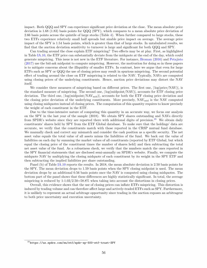
impact. Both QQQ and SPY can experience significant price deviation at the close. The mean absolute pricedeviation is 1.68 (1.83) basis points for QQQ (SPY), which compares to a mean absolute price deviation of2.66 basis points across the quintile of large stocks (Table 4). When further compared to large stocks, thesetwo ETFs experience relatively small half spreads but sizable price impact on average. The average priceimpact of the SPY is 1.54 basis points, which is greater than that of large stocks. In untabulated results, wefind that the auction deviation sensitivity to turnover is large and significant for both QQQ and SPY.

Can trading around the close explain ETF mispricing? Two effects may be at play. First, as highlightedin Table IA.10, the ETF price can substantially deviate from the midquote at the end of the day, which couldgenerate mispricing. This issue is not new in the ETF literature. For instance, Broman (2016) and Petajisto(2017) use the bid-ask midpoint to compute mispricing. However, the motivation for doing so in these papersis to mitigate concerns about the illiquidity of smaller ETFs. In contrast, here we argue that even for largeETFs such as SPY or QQQ the use of closing prices may result in spurious mispricing. The second potentialeffect of trading around the close on ETF mispricing is related to the NAV. Typically, NAVs are computedusing closing prices of the underlying constituents. Hence, auction price deviations may distort the NAVitself.

We consider three measures of mispricing based on different prices. The first one, | log(price/NAV)|, isthe standard measure of mispricing. The second one, | log(midpoint/NAV)|, accounts for ETF closing pricedeviation. The third one, | log(midpoint/NAVmid)|, accounts for both the ETF closing price deviation andthe closing price deviation of the underlying constituents. More precisely, NAVmid is the NAV computedusing closing midquotes instead of closing prices. The computation of this quantity requires to know preciselythe weight of each constituent in the ETF.

Due to the time-intensive nature of computing this quantity in an accurate way, we focus our analysison the SPY in the last year of the sample (2018). We obtain SPY shares outstanding and NAVs directlyfrom SPDR’s website since they are reported there with additional digits of precision.35 We obtain dailyconstituents’ shares held by SPY from the ETF Global database. To make sure that the holdings’ data areaccurate, we verify that the constituents match with those reported in the CRSP mutual fund database.We manually check and correct any mismatch and consider the cash position as a specific security. The netasset value equals the total value of all assets minus the liabilities of the fund. We back out the value ofliabilities on each day by summing the market values of all constituents (reported by ETF Global, but whichequal the closing price of the constituent times the number of shares held) and then subtracting the totalnet asset value of the fund. As a robustness check, we verify that the numbers match the ones reported inthe SPY financial statements that are disclosed semi-annually on SPDR’s website. Finally, we compute themidquote NAV by multiplying the closing midquote of each constituent by its weight in the SPY ETF andthen subtracting the implied liabilities per share outstanding.

Panel (b) of Table IA.10 reports the results. In 2018, the mean absolute deviation is 2.50 basis points forthe SPY. The mean deviation drops to 1.59 basis points when the SPY closing midpoint is used. The meandeviation drops by an additional 0.56 basis points once the NAV is computed using closing midquotes. Thebottom part of the panel shows that these differences are highly statistically significant. In total, the averagemispricing is reduced by 1-1.03/2.50=58.8% when taking into account the distortions in closing prices.

Overall, this evidence shows that the use of closing prices can inflate ETFs mispricing. This distortion isinduced by trading volume and can therefore affect large and actively-traded ETFs such as SPY. Furthermore,it is unlikely to represent an actual arbitrage opportunity since trading in the auction exposes an arbitrageurto both price uncertainty and execution uncertainty.

35https://us.spdrs.com/en/etf/spdr-sp-500-etf-trust-SPY

56

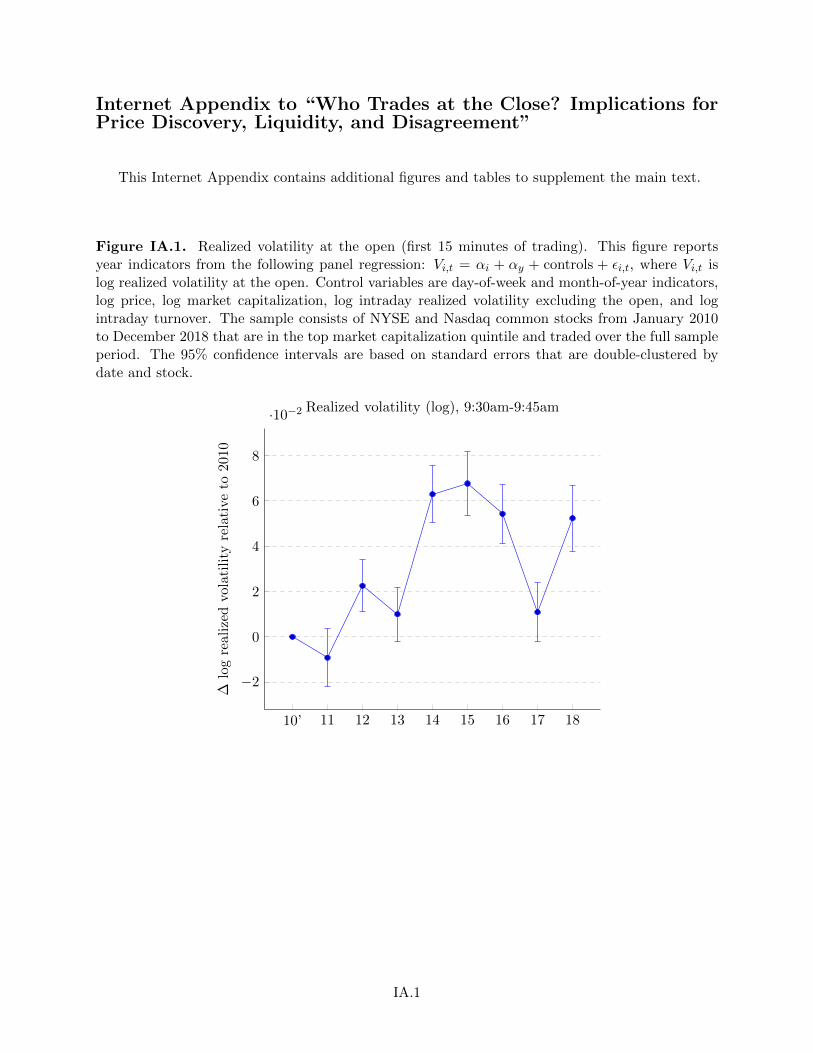
Internet Appendix to “Who Trades at the Close? Implications forPrice Discovery, Liquidity, and Disagreement”

This Internet Appendix contains additional figures and tables to supplement the main text.

Figure IA.1. Realized volatility at the open (first 15 minutes of trading). This figure reportsyear indicators from the following panel regression: Vi,t = αi + αy + controls + εi,t, where Vi,t islog realized volatility at the open. Control variables are day-of-week and month-of-year indicators,log price, log market capitalization, log intraday realized volatility excluding the open, and logintraday turnover. The sample consists of NYSE and Nasdaq common stocks from January 2010to December 2018 that are in the top market capitalization quintile and traded over the full sampleperiod. The 95% confidence intervals are based on standard errors that are double-clustered bydate and stock.

10’ 11 12 13 14 15 16 17 18

−2

0

2

4

6

8

·10−2

∆lo

gre

aliz

edvo

lati

lity

rela

tive

to201

0

Realized volatility (log), 9:30am-9:45am

IA.1

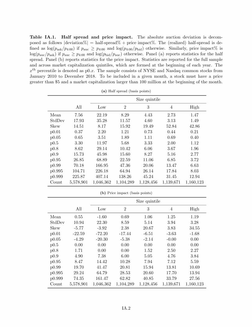
Table IA.1. Half spread and price impact. The absolute auction deviation is decom-posed as follows |deviation%| = half-spread% + price impact%. The (realized) half-spread is de-fined as log(pask/p4:00) if pauc ≥ p4:00 and log(p4:00/pbid) otherwise. Similarly, price impact% islog(pauc/pask) if pauc ≥ p4:00 and log(pbid/pauc) otherwise. Panel (a) reports statistics for the halfspread. Panel (b) reports statistics for the price impact. Statistics are reported for the full sampleand across market capitalization quintiles, which are formed at the beginning of each year. Thexth percentile is denoted as p0.x. The sample consists of NYSE and Nasdaq common stocks fromJanuary 2010 to December 2018. To be included in a given month, a stock must have a pricegreater than $5 and a market capitalization larger than 100 million at the beginning of the month.

(a) Half spread (basis points)

Size quintile

All Low 2 3 4 High

Mean 7.56 22.19 8.29 4.43 2.73 1.47StdDev 17.93 35.28 11.57 4.60 3.13 1.49Skew 14.51 8.17 15.92 19.49 52.84 42.86p0.01 0.37 2.20 1.21 0.73 0.44 0.21p0.05 0.65 3.51 1.89 1.11 0.69 0.40p0.5 3.30 11.97 5.68 3.33 2.00 1.12p0.8 8.62 29.14 10.42 6.06 3.67 1.96p0.9 15.73 45.98 15.60 8.27 5.16 2.77p0.95 26.85 68.89 22.59 11.06 6.85 3.72p0.99 70.18 166.95 47.36 20.06 13.47 6.63p0.995 104.71 226.18 64.94 26.14 17.84 8.03p0.999 225.87 407.14 138.26 45.24 31.45 12.94Count 5,578,901 1,046,362 1,104,289 1,128,456 1,139,671 1,160,123

(b) Price impact (basis points)

Size quintile

All Low 2 3 4 High

Mean 0.55 -1.60 0.69 1.06 1.25 1.19StdDev 10.94 22.30 8.59 5.14 3.94 3.28Skew -5.77 -3.92 2.38 20.67 3.83 34.55p0.01 -22.59 -72.20 -17.44 -6.51 -3.63 -1.68p0.05 -4.29 -20.30 -5.38 -2.14 -0.00 0.00p0.5 0.00 0.00 0.00 0.00 0.00 0.00p0.8 1.71 0.00 0.00 1.52 2.50 2.27p0.9 4.90 7.38 6.00 5.05 4.76 3.84p0.95 8.47 14.42 10.28 7.94 7.12 5.59p0.99 19.70 41.47 20.81 15.94 13.81 10.69p0.995 29.24 64.79 28.53 20.60 17.70 13.94p0.999 74.35 161.47 62.82 40.85 33.79 27.56Count 5,578,901 1,046,362 1,104,289 1,128,456 1,139,671 1,160,123

IA.2

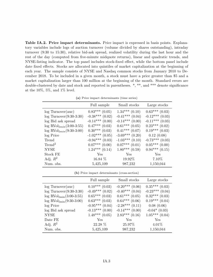
Table IA.2. Price impact determinants. Price impact is expressed in basis points. Explana-tory variables include logs of auction turnover (volume divided by shares outstanding), intradayturnover (9:30 to 15:30), relative bid-ask spread, realized volatility during the last hour and therest of the day (computed from five-minute midquote returns), linear and quadratic trends, andNYSE-listing indicator. The top panel includes stock-fixed effect, while the bottom panel includedate fixed effects. Stocks are allocated into quintiles of market capitalization at the beginning ofeach year. The sample consists of NYSE and Nasdaq common stocks from January 2010 to De-cember 2018. To be included in a given month, a stock must have a price greater than $5 and amarket capitalization larger than 100 million at the beginning of the month. Standard errors aredouble-clustered by date and stock and reported in parentheses. *, **, and *** denote significanceat the 10%, 5%, and 1% level.

(a) Price impact determinants (time series)

Full sample Small stocks Large stocks

log Turnover(auc) 0.83*** (0.05) 1.34*** (0.10) 0.63*** (0.03)log Turnover(9:30-3:30) -0.38*** (0.02) -0.41*** (0.04) -0.12*** (0.03)log Bid ask spread -0.14*** (0.00) -0.14*** (0.00) -0.11*** (0.03)log RVol5min(3:00-3:55) 0.47*** (0.03) 0.61*** (0.05) 0.23*** (0.02)log RVol5min(9:30-3:00) 0.30*** (0.03) 0.41*** (0.07) 0.19*** (0.03)log Price -1.02*** (0.05) -3.69*** (0.20) 0.12 (0.08)Trend -0.94*** (0.03) -1.03*** (0.10) -0.73*** (0.03)Trend2 0.07*** (0.00) 0.07*** (0.01) 0.05*** (0.00)NYSE 1.24*** (0.14) 1.80*** (0.59) 0.94*** (0.15)Stock FE Yes Yes YesAdj. R2 16.84 % 19.92% 7.10%Num. obs. 5,425,109 987,232 1,150,044

(b) Price impact determinants (cross-section)

Full sample Small stocks Large stocks

log Turnover(auc) 0.10*** (0.03) -0.20*** (0.06) 0.35*** (0.03)log Turnover(9:30-3:30) -0.49*** (0.02) -0.40*** (0.04) -0.23*** (0.04)log RVol5min(3:00-3:55) 0.65*** (0.03) 0.61*** (0.05) 0.32*** (0.03)log RVol5min(9:30-3:00) 0.63*** (0.03) 0.64*** (0.06) 0.19*** (0.04)log Price -0.95*** (0.04) -2.28*** (0.11) 0.08 (0.06)log Bid ask spread -0.13*** (0.00) -0.14*** (0.00) -0.04* (0.03)NYSE 1.48*** (0.05) 2.83*** (0.16) 1.05*** (0.04)Date FE Yes Yes YesAdj. R2 22.28 % 25.97% 4.01%Num. obs. 5,425,109 987,232 1,150,044

IA.3

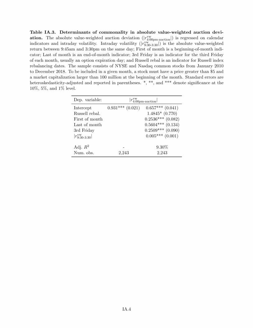
Table IA.3. Determinants of commonality in absolute value-weighted auction devi-ation. The absolute value-weighted auction deviation (|rvw

4:00pm-auction|) is regressed on calendarindicators and intraday volatility. Intraday volatility (|rvw

9:30-3:30|) is the absolute value-weightedreturn between 9:45am and 3:30pm on the same day; First of month is a beginning-of-month indi-cator; Last of month is an end-of-month indicator; 3rd Friday is an indicator for the third Fridayof each month, usually an option expiration day; and Russell rebal is an indicator for Russell indexrebalancing dates. The sample consists of NYSE and Nasdaq common stocks from January 2010to December 2018. To be included in a given month, a stock must have a price greater than $5 anda market capitalization larger than 100 million at the beginning of the month. Standard errors areheteroskedasticity-adjusted and reported in parentheses. *, **, and *** denote significance at the10%, 5%, and 1% level.

Dep. variable: |rvw4:00pm-auction|

Intercept 0.931*** (0.021) 0.657*** (0.041)Russell rebal. 1.4845* (0.770)First of month 0.2536*** (0.082)Last of month 0.5604*** (0.134)3rd Friday 0.2509*** (0.090)|rvw

9:30-3:30| 0.005*** (0.001)

Adj. R2 - 9.30%Num. obs. 2,243 2,243

IA.4

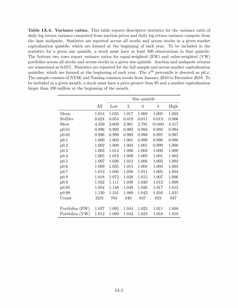
Table IA.4. Variance ratios. This table reports descriptive statistics for the variance ratio ofdaily log return variance computed from auction prices and daily log return variance compute fromthe 4pm midquote. Statistics are reported across all stocks and across stocks in a given marketcapitalization quintile, which are formed at the beginning of each year. To be included in thestatistics for a given size quintile, a stock must have at least 500 observations in that quintile.The bottom two rows report variance ratios for equal-weighted (EW) and value-weighted (VW)portfolios across all stocks and across stocks in a given size quintile. Auction and midquote returnsare winsorized at 0.05%. Statistics are reported for the full sample and across market capitalizationquintiles, which are formed at the beginning of each year. The xth percentile is denoted as p0.x.The sample consists of NYSE and Nasdaq common stocks from January 2010 to December 2018. Tobe included in a given month, a stock must have a price greater than $5 and a market capitalizationlarger than 100 million at the beginning of the month.

Size quintile

All Low 2 3 4 High

Mean 1.014 1.045 1.017 1.008 1.005 1.003StdDev 0.024 0.054 0.019 0.011 0.013 0.006Skew 4.359 2.609 2.961 2.785 10.694 4.517p0.01 0.996 0.992 0.992 0.994 0.993 0.994p0.05 0.998 0.999 0.999 0.998 0.997 0.997p0.1 1.000 1.003 1.001 0.999 0.998 0.998p0.2 1.002 1.009 1.003 1.001 0.999 1.000p0.3 1.003 1.014 1.006 1.003 1.000 1.000p0.4 1.005 1.019 1.009 1.005 1.001 1.002p0.5 1.007 1.026 1.012 1.006 1.002 1.002p0.6 1.009 1.035 1.015 1.008 1.004 1.003p0.7 1.013 1.050 1.020 1.011 1.005 1.004p0.8 1.018 1.072 1.026 1.015 1.007 1.006p0.9 1.032 1.111 1.039 1.020 1.012 1.009p0.95 1.054 1.148 1.049 1.026 1.017 1.012p0.99 1.130 1.241 1.089 1.042 1.034 1.021Count 2231 704 840 847 823 647

Portfolios (EW) 1.037 1.095 1.044 1.025 1.011 1.008Portfolios (VW) 1.012 1.089 1.042 1.024 1.010 1.010

IA.5

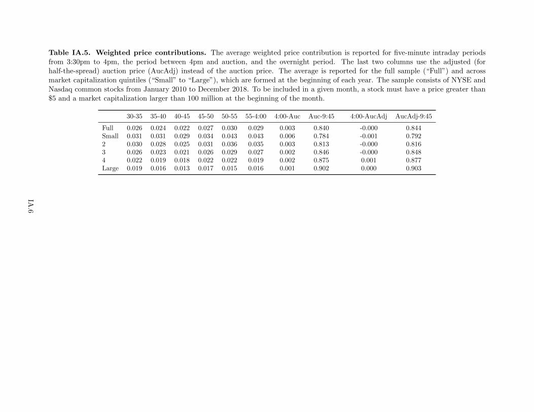
Table IA.5. Weighted price contributions. The average weighted price contribution is reported for five-minute intraday periodsfrom 3:30pm to 4pm, the period between 4pm and auction, and the overnight period. The last two columns use the adjusted (forhalf-the-spread) auction price (AucAdj) instead of the auction price. The average is reported for the full sample (“Full”) and acrossmarket capitalization quintiles (“Small” to “Large”), which are formed at the beginning of each year. The sample consists of NYSE andNasdaq common stocks from January 2010 to December 2018. To be included in a given month, a stock must have a price greater than$5 and a market capitalization larger than 100 million at the beginning of the month.

30-35 35-40 40-45 45-50 50-55 55-4:00 4:00-Auc Auc-9:45 4:00-AucAdj AucAdj-9:45

Full 0.026 0.024 0.022 0.027 0.030 0.029 0.003 0.840 -0.000 0.844Small 0.031 0.031 0.029 0.034 0.043 0.043 0.006 0.784 -0.001 0.7922 0.030 0.028 0.025 0.031 0.036 0.035 0.003 0.813 -0.000 0.8163 0.026 0.023 0.021 0.026 0.029 0.027 0.002 0.846 -0.000 0.8484 0.022 0.019 0.018 0.022 0.022 0.019 0.002 0.875 0.001 0.877Large 0.019 0.016 0.013 0.017 0.015 0.016 0.001 0.902 0.000 0.903

IA.6

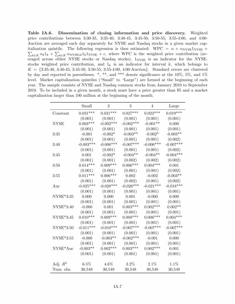
Table IA.6. Dissemination of closing information and price discovery. Weightedprice contributions between 3:30-35, 3:35-40, 3:40-45, 3:45-50, 3:50-55, 3:55-4:00, and 4:00-Auction are averaged each day separately for NYSE and Nasdaq stocks in a given market cap-italization quintile. The following regression is then estimated: WPC = α + αNYSE1NYSE +∑

k∈K αk1k +∑

k∈K αNYSE∗k1k1NYSE + ε, where WPC is the weighted price contribution (av-eraged across either NYSE stocks or Nasdaq stocks), 1NYSE is an indicator for the NYSE-stocks weighted price contribution, and 1k is an indicator for interval k, which belongs toK = {3:35-40, 3:40-45, 3:45-50, 3:50-55, 3:55-4:00, 4:00-Auction}. Standard errors are clusteredby day and reported in parentheses. *, **, and *** denote significance at the 10%, 5%, and 1%level. Market capitalization quintiles (“Small” to “Large”) are formed at the beginning of eachyear. The sample consists of NYSE and Nasdaq common stocks from January 2010 to September2018. To be included in a given month, a stock must have a price greater than $5 and a marketcapitalization larger than 100 million at the beginning of the month.

Small 2 3 4 Large

Constant 0.031*** 0.031*** 0.027*** 0.023*** 0.019***(0.001) (0.001) (0.001) (0.001) (0.001)

NYSE 0.003*** -0.002*** -0.002*** -0.001** 0.000(0.001) (0.001) (0.001) (0.001) (0.001)

3:35 -0.001 -0.002* -0.003** -0.002* -0.003**(0.001) (0.001) (0.001) (0.001) (0.002)

3:40 -0.003*** -0.006*** -0.007*** -0.006*** -0.007***(0.001) (0.001) (0.001) (0.001) (0.002)

3:45 0.001 -0.002* -0.004** -0.004** -0.004***(0.001) (0.001) (0.002) (0.002) (0.002)

3:50 0.014*** 0.009*** 0.006*** 0.004*** 0.001(0.001) (0.001) (0.001) (0.001) (0.002)

3:55 0.011*** 0.006*** 0.002 -0.002 -0.003**(0.001) (0.001) (0.002) (0.001) (0.002)

Auc -0.025*** -0.028*** -0.026*** -0.021*** -0.018***(0.001) (0.001) (0.001) (0.001) (0.001)

NYSE*3:35 0.000 0.000 0.001 -0.000 0.000(0.001) (0.001) (0.001) (0.001) (0.001)

NYSE*3:40 -0.000 0.001 0.003*** 0.002*** 0.002**(0.001) (0.001) (0.001) (0.001) (0.001)

NYSE*3:45 0.010*** 0.009*** 0.008*** 0.006*** 0.004***(0.001) (0.001) (0.001) (0.001) (0.001)

NYSE*3:50 -0.011*** -0.010*** -0.007*** -0.007*** -0.007***(0.001) (0.001) (0.001) (0.001) (0.001)

NYSE*3:55 -0.000 -0.003** -0.002*** -0.001 0.000(0.001) (0.001) (0.001) (0.001) (0.001)

NYSE*Auc -0.003** 0.002*** 0.003*** 0.002*** 0.001(0.001) (0.001) (0.001) (0.001) (0.001)

Adj. R2 6.5% 4.6% 3.2% 2.1% 1.1%Num. obs. 30,548 30,548 30,548 30,548 30,548

IA.7

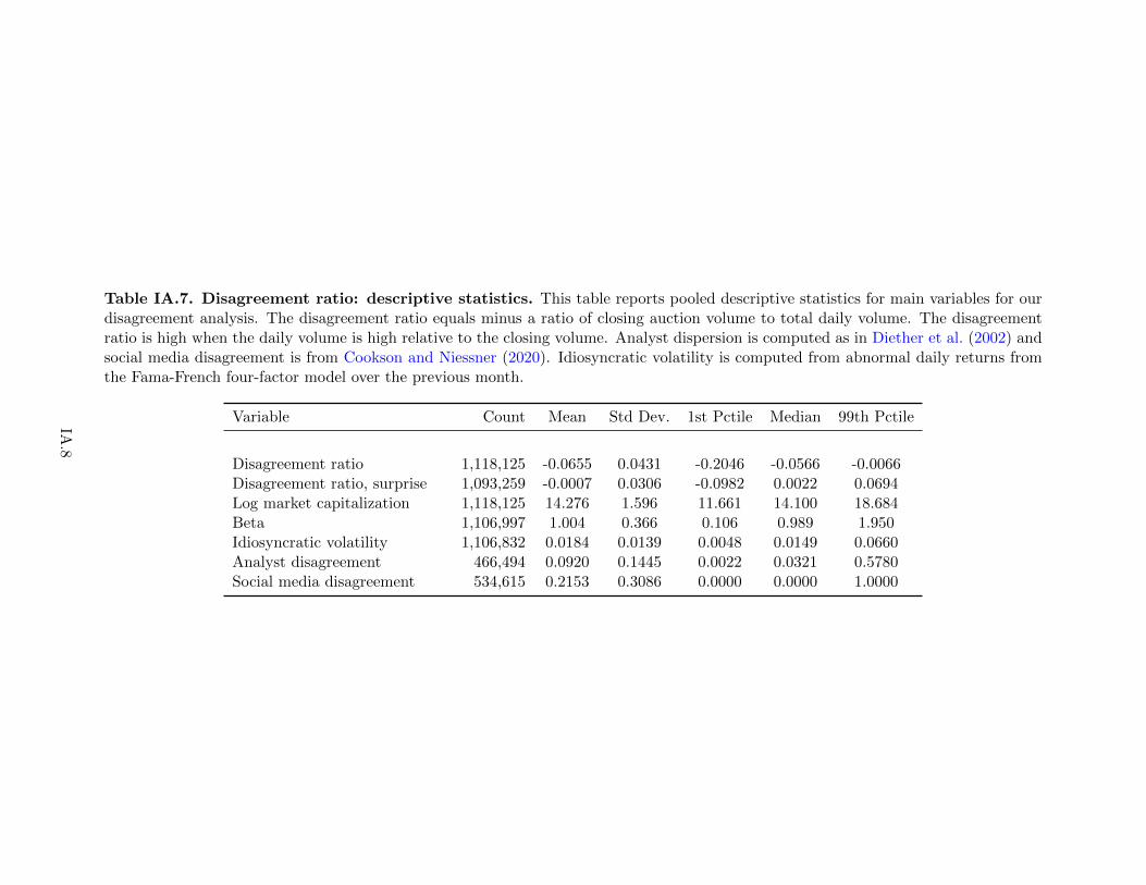
Table IA.7. Disagreement ratio: descriptive statistics. This table reports pooled descriptive statistics for main variables for ourdisagreement analysis. The disagreement ratio equals minus a ratio of closing auction volume to total daily volume. The disagreementratio is high when the daily volume is high relative to the closing volume. Analyst dispersion is computed as in Diether et al. (2002) andsocial media disagreement is from Cookson and Niessner (2020). Idiosyncratic volatility is computed from abnormal daily returns fromthe Fama-French four-factor model over the previous month.

Variable Count Mean Std Dev. 1st Pctile Median 99th Pctile

Disagreement ratio 1,118,125 -0.0655 0.0431 -0.2046 -0.0566 -0.0066Disagreement ratio, surprise 1,093,259 -0.0007 0.0306 -0.0982 0.0022 0.0694Log market capitalization 1,118,125 14.276 1.596 11.661 14.100 18.684Beta 1,106,997 1.004 0.366 0.106 0.989 1.950Idiosyncratic volatility 1,106,832 0.0184 0.0139 0.0048 0.0149 0.0660Analyst disagreement 466,494 0.0920 0.1445 0.0022 0.0321 0.5780Social media disagreement 534,615 0.2153 0.3086 0.0000 0.0000 1.0000

IA.8

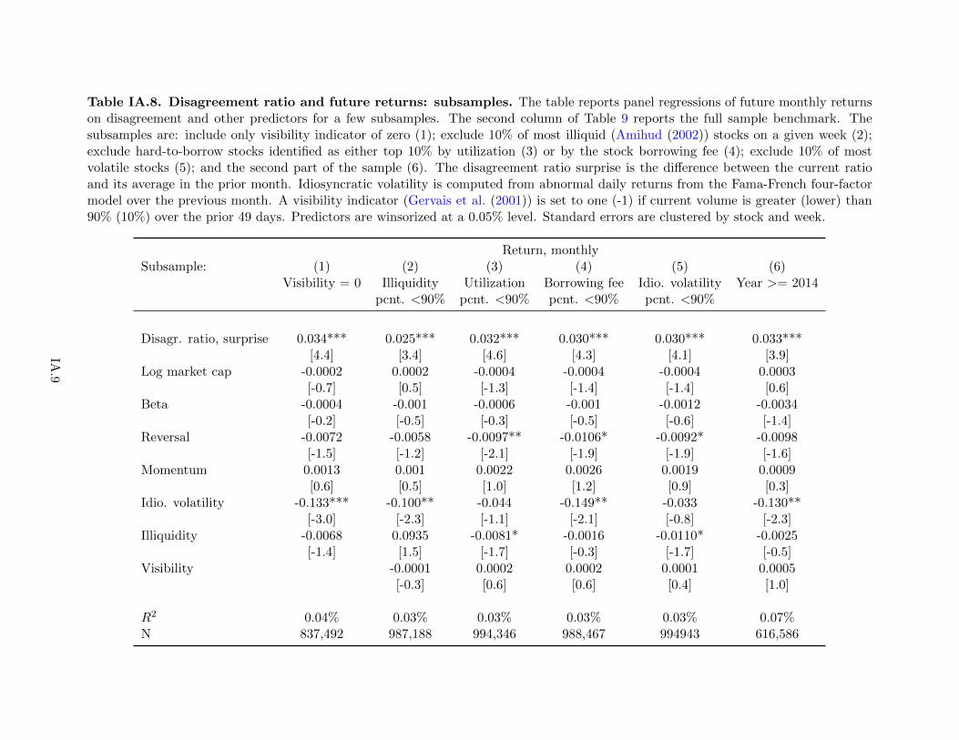
Table IA.8. Disagreement ratio and future returns: subsamples. The table reports panel regressions of future monthly returnson disagreement and other predictors for a few subsamples. The second column of Table 9 reports the full sample benchmark. Thesubsamples are: include only visibility indicator of zero (1); exclude 10% of most illiquid (Amihud (2002)) stocks on a given week (2);exclude hard-to-borrow stocks identified as either top 10% by utilization (3) or by the stock borrowing fee (4); exclude 10% of mostvolatile stocks (5); and the second part of the sample (6). The disagreement ratio surprise is the difference between the current ratioand its average in the prior month. Idiosyncratic volatility is computed from abnormal daily returns from the Fama-French four-factormodel over the previous month. A visibility indicator (Gervais et al. (2001)) is set to one (-1) if current volume is greater (lower) than90% (10%) over the prior 49 days. Predictors are winsorized at a 0.05% level. Standard errors are clustered by stock and week.

Return, monthlySubsample: (1) (2) (3) (4) (5) (6)

Visibility = 0 Illiquidity Utilization Borrowing fee Idio. volatility Year >= 2014pcnt. <90% pcnt. <90% pcnt. <90% pcnt. <90%

Disagr. ratio, surprise 0.034*** 0.025*** 0.032*** 0.030*** 0.030*** 0.033***[4.4] [3.4] [4.6] [4.3] [4.1] [3.9]

Log market cap -0.0002 0.0002 -0.0004 -0.0004 -0.0004 0.0003[-0.7] [0.5] [-1.3] [-1.4] [-1.4] [0.6]

Beta -0.0004 -0.001 -0.0006 -0.001 -0.0012 -0.0034[-0.2] [-0.5] [-0.3] [-0.5] [-0.6] [-1.4]

Reversal -0.0072 -0.0058 -0.0097** -0.0106* -0.0092* -0.0098[-1.5] [-1.2] [-2.1] [-1.9] [-1.9] [-1.6]

Momentum 0.0013 0.001 0.0022 0.0026 0.0019 0.0009[0.6] [0.5] [1.0] [1.2] [0.9] [0.3]

Idio. volatility -0.133*** -0.100** -0.044 -0.149** -0.033 -0.130**[-3.0] [-2.3] [-1.1] [-2.1] [-0.8] [-2.3]

Illiquidity -0.0068 0.0935 -0.0081* -0.0016 -0.0110* -0.0025[-1.4] [1.5] [-1.7] [-0.3] [-1.7] [-0.5]

Visibility -0.0001 0.0002 0.0002 0.0001 0.0005[-0.3] [0.6] [0.6] [0.4] [1.0]

R2 0.04% 0.03% 0.03% 0.03% 0.03% 0.07%N 837,492 987,188 994,346 988,467 994943 616,586

IA.9

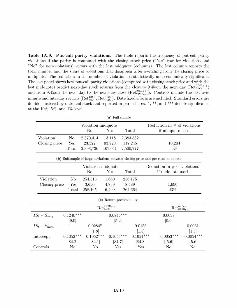
Table IA.9. Put-call parity violations. The table reports the frequency of put-call parityviolations if the parity is computed with the closing stock price (”Yes” row for violations and”No” for non-violations) versus with the last midquote (columns). The last column reports thetotal number and the share of violations that disappear after switching from the closing price tomidquote. The reduction in the number of violations is statistically and economically significant.The last panel shows how put-call parity violations (computed with closing stock price and with thelast midquote) predict next-day stock returns from the close to 9:45am the next day (Ret

opent+1auct )

and from 9:45am the next day to the next-day close (Retauct+1opent+1

). Controls include the last five-

minute and intraday returns (Ret4:00t3:55t

, Ret3:55t9:35t

). Date fixed effects are included. Standard errors aredouble-clustered by date and stock and reported in parentheses. *, **, and *** denote significanceat the 10%, 5%, and 1% level.

(a) Full sample

Violation midquote Reduction in # of violationsNo Yes Total if midquote used

Violation No 2,370,414 13,118 2,383,532Closing price Yes 23,322 93,923 117,245 10,204

Total 2,393,736 107,041 2,500,777 9%

(b) Subsample of large deviations between closing price and pre-close midquote

Violation midquote Reduction in # of violationsNo Yes Total if midquote used

Violation No 254,515 1,660 256,175Closing price Yes 3,650 4,839 8,489 1,990

Total 258,165 6,499 264,664 23%

(c) Return predictability

Retopent+1auct Ret

auct+1opent+1

ISt − Sauct 0.1240*** 0.0845*** 0.0098[9.0] [5.2] [0.9]

ISt − Smidt 0.0284* 0.0156 0.0061[1.8] [1.5] [1.5]

Intercept 0.1052*** 0.1052*** 0.1054*** 0.1054*** -0.0053*** -0.0054***[84.2] [84.1] [84.7] [84.8] [-5.6] [-5.6]

Controls No No Yes Yes No No

IA.10

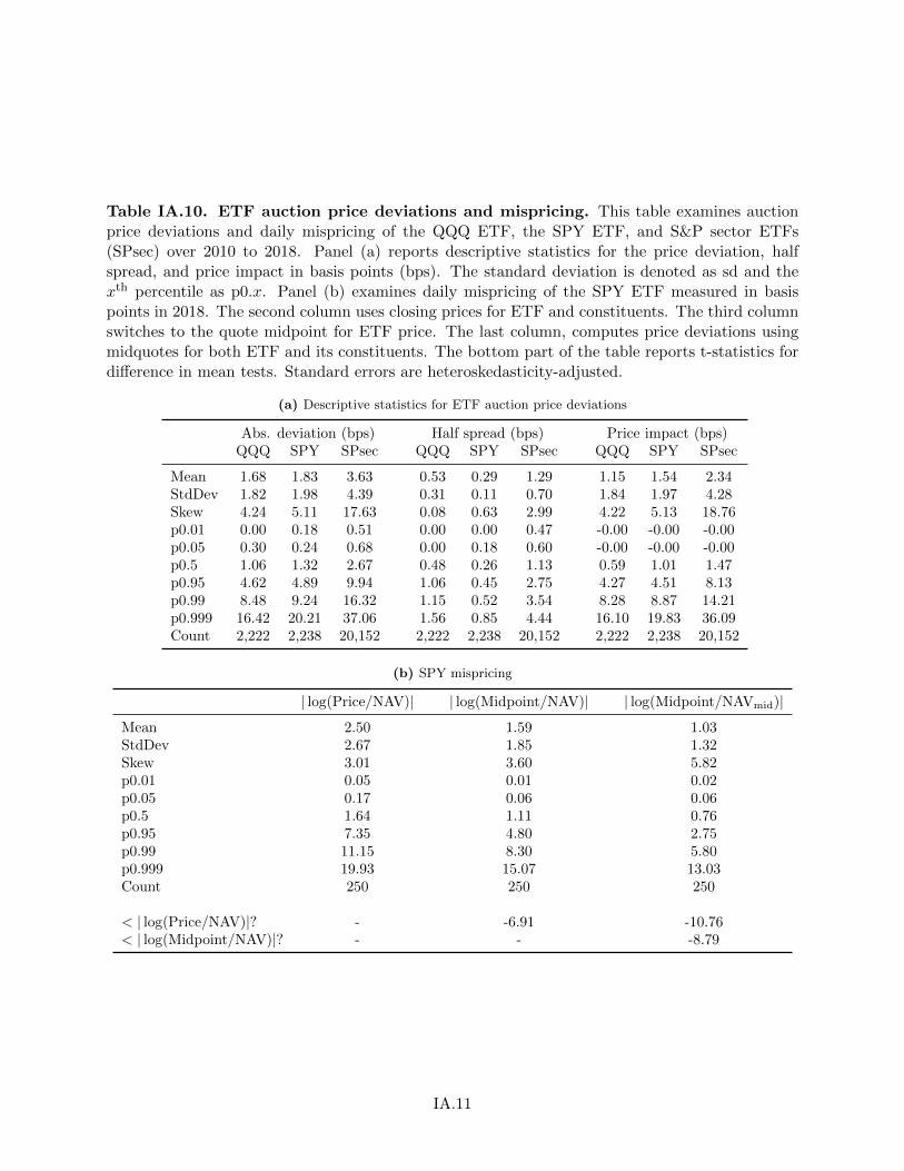
Table IA.10. ETF auction price deviations and mispricing. This table examines auctionprice deviations and daily mispricing of the QQQ ETF, the SPY ETF, and S&P sector ETFs(SPsec) over 2010 to 2018. Panel (a) reports descriptive statistics for the price deviation, halfspread, and price impact in basis points (bps). The standard deviation is denoted as sd and thexth percentile as p0.x. Panel (b) examines daily mispricing of the SPY ETF measured in basispoints in 2018. The second column uses closing prices for ETF and constituents. The third columnswitches to the quote midpoint for ETF price. The last column, computes price deviations usingmidquotes for both ETF and its constituents. The bottom part of the table reports t-statistics fordifference in mean tests. Standard errors are heteroskedasticity-adjusted.

(a) Descriptive statistics for ETF auction price deviations

Abs. deviation (bps) Half spread (bps) Price impact (bps)QQQ SPY SPsec QQQ SPY SPsec QQQ SPY SPsec

Mean 1.68 1.83 3.63 0.53 0.29 1.29 1.15 1.54 2.34StdDev 1.82 1.98 4.39 0.31 0.11 0.70 1.84 1.97 4.28Skew 4.24 5.11 17.63 0.08 0.63 2.99 4.22 5.13 18.76p0.01 0.00 0.18 0.51 0.00 0.00 0.47 -0.00 -0.00 -0.00p0.05 0.30 0.24 0.68 0.00 0.18 0.60 -0.00 -0.00 -0.00p0.5 1.06 1.32 2.67 0.48 0.26 1.13 0.59 1.01 1.47p0.95 4.62 4.89 9.94 1.06 0.45 2.75 4.27 4.51 8.13p0.99 8.48 9.24 16.32 1.15 0.52 3.54 8.28 8.87 14.21p0.999 16.42 20.21 37.06 1.56 0.85 4.44 16.10 19.83 36.09Count 2,222 2,238 20,152 2,222 2,238 20,152 2,222 2,238 20,152

(b) SPY mispricing

| log(Price/NAV)| | log(Midpoint/NAV)| | log(Midpoint/NAVmid)|

Mean 2.50 1.59 1.03StdDev 2.67 1.85 1.32Skew 3.01 3.60 5.82p0.01 0.05 0.01 0.02p0.05 0.17 0.06 0.06p0.5 1.64 1.11 0.76p0.95 7.35 4.80 2.75p0.99 11.15 8.30 5.80p0.999 19.93 15.07 13.03Count 250 250 250

< | log(Price/NAV)|? - -6.91 -10.76< | log(Midpoint/NAV)|? - - -8.79

IA.11