Wharton-SMU Research Center A MARKOV CHAINS IN PREDICTIVE MODELS OF CURRENCY CRISES - WITH APPLICATIONS TO SOUTHEAST ASIA

Wharton-SMU Research Center

A MARKOV CHAINS IN PREDICTIVE MODELS OF CURRENCY CRISES – WITH

APPLICATIONS TO SOUTHEAST ASIA

Roberto S. Mariano, Abdul G. Abiad, Bulent Gultekin,

Tayyeb Shabbir and Augustine H. H. Tan

(May 2002)

This project is funded by the Wharton-SMU Research Center of Singapore Management University

MARKOV CHAINS IN PREDICTIVE MODELS OF CURRENCY CRISES – WITH APPLICATIONS TO SOUTHEAST ASIA

Roberto S. Mariano*, Abdul G. Abiad***, Bulent Gultekin*, Tayyeb Shabbir* and Augustine H. H. Tan**

May 2002

This research has been supported in part by a grant from the Wharton-Singapore Management University Research Center. The authors gratefully acknowledge the research assistance provided by Sean Campbell and Melissa Tartari. *University of Pennsylvania **Singapore Management University *** International Monetary Fund

1

MARKOV CHAINS IN PREDICTIVE MODELS OF CURRENCY CRISES – WITH APPLICATIONS TO SOUTHEAST ASIA

Roberto S. Mariano, Abdul G. Abiad, Bulent Gultekin, Tayyeb Shabbir and Augustine Tan

May 2002

INTRODUCTION AND SUMMARY The decade of the 1990s was marked by an unusual number of financial and economic crises such as the attack on the European Monetary System in 1992-93, the Mexican peso crisis in 1994-95, the Asian crisis in 1997, the Russian default in 1998 and its spillover to Latin America. The Turkish currency and banking crisis in 2001 and the recent difficulties in Argentina indicate that financial crises are still part of the current economic events. In the wake of such developments, there has been a resurgence of interest in early warning systems that can anticipate the likely occurrence of such crises. There is an extensive literature on the Asian financial crisis and early warning systems – with numerous surveys including Goldstein (1998), Montes (1998), McLeod and Garnaut (1998), Kaminsky and Reinhart (1998), Tan (1998, 1999), Mariano, Gultekin, Ozmucur and Shabbir (1999), Goldstein, Kaminsky and Reinhart (2000), Richterr (2000), and Abiad (2002). Along these lines, this paper explores the issue of constructing a monthly economic predictive model of currency crises in Southeast Asia through an alternative econometric methodology that addresses drawbacks in existing approaches. Our methodology entails estimating a Markov regime switching model of exchange rate movements, with time-varying transition probabilities. In this paper, we discuss the technical details involved in this approach and apply it to Indonesia, Malaysia, the Philippines and Thailand. Our approach is designed to avoid the potential misclassification in the construction of crisis dummy variables which other approaches (such as probit/logit and signalling) require. Our methodology also addresses the serial correlations and sudden behavior inherent in crisis occurrence, identifies a set of reliable and observable indicators of impending currency difficulties, delivers forecast probabilities of future crises over multi-period forecasting horizons, and offers an empirical framework for analyzing contagion effects of a crisis and for improving short-run forecasts of key macroeconomic variables. The preliminary results reported in the paper are based on estimated univariate two-state Markov switching models of monthly percentage changes in nominal exchange rates. Transition probabilities in the Markov chains are affected by deviations of the real effective exchange rate from trend, percentage changes in the ratio of money supply to international reserves, and percentage changes in real domestic credit. Our results indicate that the basic Markov switching model is moderately successful at identifying currency crisis episodes - with some success in predicting the recent crisis in Thailand and Malaysia. For all countries studied, exchange rate behavior can be characterized into two regimes - one with zero mean and low volatility in exchange rate percentage changes; and another with positive mean (currency depreciation) and high volatility. Real exchange rate overvaluation (relative to trend) is an important explanatory variable for predicting a switch from a low volatility to a high volatility period; it is correctly signed for all four countries and is statistically significant in the case of Malaysia and Thailand. The two other early warning indicators explored in our analysis - growth in real domestic credit and in money supply relative to reserves - showed only moderate importance, entering into the final specifications only in selected countries. The models proved moderately successful at sending warning signals but the results are not uniform across countries. For some depreciation episodes, like those in 1981 and 1984 for Thailand as well as the 1997 crisis for both Malaysia and Thailand, the model provides strong signals, in some cases, several months in advance. But for other episodes, such as the 1997 crisis episodes for Indonesia and the Philippines, the model provides at best only weak warning signals.

2

These initial results point to future research work in various directions:

• A more extensive search for macroeconomic indicators in the transition probabilities and use of sector indicators such as non-performing loans in the banking sector and short-term flows in financial markets,

• Technical enhancement of the model with more states in the Markov chain (distinguishing

conditions leading to a strong currency) and duration dependence in the transition probabilities,

• Modeling exchange rate movements jointly with interest rates and reserves through a Markov

regime switching VAR model,

• Including key macroeconomic variables, such as inflation and output, in the individual country VAR models - to improve short-term forecasting , not only of a currency crisis, but also inflation and output,

• A Markov switching VAR model combining countries into one inter-related model to analyze

the contagion effects of a currency crisis,

• Formal statistical procedures to assess the forecasting performance of the Markov switching model, and

• Alternative econometric models such as ARCH and latent common factor dynamic models.

CURRENCY CRISIS THEORY The theoretical literature on currency crises can be broken up loosely into three “generations”, delineated by the underlying mechanism that brings about the crisis. The first generation focuses on “fundamentals,” and emphasizes the role of unsustainable government policies that are incompatible with a pegged exchange rate, and which eventually lead to its collapse. The canonical model here was presented in Krugman (1979) , based on a government that is financing persistent budget deficits through monetization. This simplest of models suggests that in the period leading up to a speculative attack, one should notice a gradual decline in reserves. It also suggests that budget deficits and growth in domestic credit may be potential early warning indicators for speculative attacks. Extensions of the basic model look at the other factors that may force the government to abandon the peg. For example, expansionary policy may lead directly to a worsening of the current account through a rise in import demand; the same result may occur indirectly through a rise in the price of nontradeables and the subsequent overvaluation of the real exchange rate. Thus, the behavior of external variables such as the current account deficit and the real exchange rate may provide some warning regarding the vulnerability of a country to a speculative attack. Second-generation models were motivated by episodes such as the ERM crisis in 1992-93, where some of the countries did not seem to possess the characteristics described in first-generation models. This led researchers such as Obstfeld (1994) to enrich existing theories of currency crises. The key element in second generation models is a recognition that there are both benefits and costs to maintaining a peg, and that market participant’s beliefs over whether a peg will hold or not can affect the government’s cost of defending it. The circularity inherent in second-generation models – that government policy is affected by expectations, and expectations are affected by government policy – leads to the possibility of multiple equilibria and self-fulfilling crises. These second-generation models suggest that anything that affects a government’s decision whether to maintain a peg or not – unemployment, inflation, the amount and composition of debt, financial sector stability, etc. – might contain information on the likelihood of a crisis occurring. The third generation of currency crisis models focuses on the issue of contagion, or why the occurrence of a crisis in one country seems to affect the likelihood of a crisis occurring in other countries. Masson (1998)

3

suggests three possible reasons why crises seem to come in clusters. First, there may actually be common external shocks (e.g. fluctuations in world interest rates) that affect all the countries involved. Second, there may be spillover effects from one country to another due to trade competitiveness effects or portfolio rebalancing effects. Lastly, speculative attacks might spread from country to country merely on the basis of market sentiment or herding behavior. This class of models suggests that early warning systems should include external variables such as LIBOR or the growth rate of trading partners; they also imply that the occurrence of a crisis in a trading partner or in “similar countries” should be taken into account. EARLY WARNING SYSTEMS Recent efforts (Eichengreen and Rose, 1998; Demigurc-Kunt and Detragiache, 1998; Kaminsky and Reinhart, 1996 and 1998; Kaminsky, Lizondo and Reinhart, 1998; and IMF, 1998a and 1998b) towards devising an early warning system for an impending financial crisis have taken two related forms. The first approach estimates a probit or logit model of the occurrence of a crisis with lagged values of early warning indicators as explanatory variables. This approach requires the construction of a crisis dummy variable that serves as the endogenous variable in the probit or logit regression. Classification of each sample time-point as being in crisis or not depends on whether or not a specific index of vulnerability or speculative pressure exceeds a chosen threshold. For currency crises, the index of vulnerability is often based on a weighted average of the following three variables:

• percentage changes in nominal exchange rates • percentage change in gross international reserves • difference in local and foreign short-term interest rates.

Explanatory variables typically come from the real, financial, external and fiscal sectors of the economy. The second method uses a signalling or leading-indicator approach to get a more direct measure of the importance of each candidate explanatory variable. Apart from constructing a crisis dummy variable, the approach also constructs binary variables from each explanatory variable – thus imputing a value of one (a “signal”) or zero (no signal) for each explanatory variable at each point in time in the sample – based on whether each variable exceeds a chosen threshold or not. These signals are classified according to their ability to call a crisis: a signal is a “good signal” if a crisis does ensue within a specified period (usually 24 months), and is a “false signal” otherwise. Thresholds are chosen so as to strike a balance between the risk of having many false signals and the risk of missing many crises. More precisely, a signal-to-noise ratio is computed for each explanatory variable over the sample period – as a quantitative assessment of the value of the variable as a crisis indicator. This is done by classifying each observation of the binary signalling variable into one of the following four categories:

Crisis occurs within 24 months No crisis occurs within 24 months Signal A B No Signal C D

Thresholds are then chosen to maximize the signal-to-noise ratio [A/(A+C)]/[B/(B+D)]. Based on this metric, Kaminsky, Reinhart and Lizondo (1998) find that the best early warning indicators for currency crises include exports, deviations of the real exchange rate from trend, M2/reserves, output, and equity prices. Whether this approach or a probit/logit approach is used, to cover a wider sample for purposes of estimating incidence probabilities for a crisis, many studies have been typically done on a panel of countries – and usually with some homogeneity assumptions about crisis behavior across countries.

4

Drawbacks in Current Approaches Despite the current popularity of these approaches, they have some drawbacks, which include the following (see Abiad (1999) and Mariano (1999) for a more detailed discussion):

• Inadequate treatment of serial correlations inherent in the dynamics of a crisis. Neither the probit/logit approach nor the signalling approach gives us information on dynamics – how long crisis periods tend to last – nor do they give information about what variables affect the likelihood of a crisis period ending.

• Artificial serial correlations may even be introduced inadvertently through the explicit manner

in which the crisis dummy variable is constructed. Many previous studies focus primarily on predicting the onset of a crisis, i.e. the first period where speculative attacks occur. To achieve this in their binary crisis variable, they make use of so-called “exclusion windows” which remove any crisis signals that closely follow previous crisis signals. This procedure can introduce artificial serial correlations; see Abiad (1999).

• Classification errors may result when constructing the crisis dummy variable (either as a false

signal of a crisis, or a missed reading of a crisis). Because the threshold used to delineate crisis periods from tranquil periods is arbitrarily chosen, misclassification of crisis episodes can occur. If the threshold is too high, for example, some periods of vulnerability may not be picked up.

• Inadequate framework for significance testing of the influence of explanatory or indicator

variables (in the signalling approach). Because the signalling approach is not based on an explicit stochastic model, there is no way it can be evaluated using formal statistical tests, and it is difficult to assess its performance vis-à-vis other approaches.

• Possible inconsistencies in the estimation of crisis incidence probabilities because of

heterogeneity across countries. It is possible that the variables which are important in determining crisis likelihoods for one country are unimportant for another country. And even if the same variables affected crisis likelihoods for all countries, the degree to which affects the likelihood of a crisis occuring may differ from one country to the next.

Our Approach We apply a new early warning methodology that addresses these drawbacks. We construct for each individual country a Markov switching autoregressive model that allows intercepts, lag coefficients and error variances to stochastically switch over time according to the value taken by a latent Markov chain describing the vulnerability of the country’s currency to speculative attacks. A related work, Martinez (1999), also applies a Markov-switching model to speculative attacks, but the primary purpose in that paper was to evaluate the ability of the model in dating crisis periods and to see whether market expectations affected crisis probabilities. Here the focus is on the use of the model as an early warning system. Thus our predictive model of a currency crisis consists of two parts:

1. A Markov chain model of the unobservable financial vulnerability of the country, say St. We argue that what we observe are indicators of this latent attribute of the country. Initially, we assume two states:

• normal (St = 0)

• vulnerable (S t = 1).

5

We further assume that this Markov chain is of order 1, with transition probabilities that are time-varying through dependence on observable indicator variables. The preliminary results we report in this paper are based on the following indicator variables:

• deviations of real effective exchange rate from trend • month-to-month percentage changes in the ratio of M2 to international reserves

• month-to-month percentage changes in real domestic credit.

2. A Markov regime-switching time series model of percentage changes in nominal exchange

rates. This model differs from standard ones in the sense that it includes the unobservable state variable St as an additional endogenous variable. With the inclusion of St, we introduce the notion that the exchange rate dynamics behaves in a different fashion depending on whether financial conditions are normal (St = 0) or vulnerable to currency pressures (St = 1). We reflect this in our model by allowing the parameters in our time-series model to change in value over time, as financial conditions become normal or vulnerable.

Our Model in Detail Let St be a two-state Markov chain of order 1 with transition probabilities pt and qt, so that at any given time t, St can take on two values, zero or one, according to the following probability law: Pr(St = 0 St-1 = 0) = pt and Pr(St = 1 St-1 = 1) = qt. Further, let yt = month-to-month percentage changes in nominal exchange rates, xt = the vector of exogenous variables at time t to be used to explain yt, zt = the vector of exogenous variables at time t to be used as indicators of currency vulnerability, which may overlap with xt. We assume also that the transition probabilities vary over time according to values of indicator variables in the following manner:

pt = F(zt’γ) and qt = F(zt’δ),

where F(•) is the standard unit Gaussian cumulative distribution function. The second part of the model consists of a univariate linear model for yt: yt = αSt + xt’βSt + σSt εt. In this model, the model parameters (α, β, σ) are subscripted by St – indicating that their true (unknown) values are shifting between two sets of possible parameter values: (α0, β0, σo) and (α1, β1, σ1) depending on whether financial conditions are normal or vulnerable. The estimation procedure we use is direct maximization of the likelihood, where the likelihood function is calculated using an iterative process, described in detail in Hamilton (1994). Collect all the parameters of

6

the model into a single vector θ = (α0, β0, σ0, α1, β1, σ1, γ’, δ’). Using information available up to time t, Ωt, we can calculate for each time t (using the iteration below) the value of );θtt js Ω=Pr( , the conditional probability that the tth observation was generated by regime j, for j = 1,2,…N, where N is the number of states (in this paper, N=2). We will stack these conditional probabilities into an (Nx1) vector . tt|ξ

Using the same iteration, we can also form forecasts regarding the conditional probability of being in regime j at time t+1, given information up to time t: );Pr( 1 θtt js Ω=+

t

, for j = 1,2,…N. Collect these

forecast probabilities in an (Nx1) vector . Lastly, let tt |1ˆ

+ξ η denote the (Nx1) vector whose jth element is the density of yt conditional on st.

The optimal inference and forecast for each date t can then be found by iterating on the following equations:

)ˆ(

)ˆ(ˆ1|

1||

ttt

ttttt ηξ

ηξξ

o

o

−

−

′=

1

ttttt |1|1ˆˆ ξξ ⋅= ++ P

where Pt is the (NxN) transition probability matrix going from period t-1 to period t (for the 2-state model in this paper, Pt is the 2x2 matrix [pt 1-pt ; 1-qt qt] ), and ° denotes element-by-element multiplication. Given an assumed value for the parameters, θ, and an assumed starting value for (the unconditional

probability of s

0|1ξ

tξt at t=1), we can then iterate on the above equations to obtain values of and for t = 1,2,…T. The log likelihood function L(θ) can be computed from these as

t| tt |1ˆ

+ξ

∑=

−=T

tttt YXyfL

11 );,|(log)( θθ

where )ˆ(1);,|( |1 tttttt YXyf ηξθ o′=− .

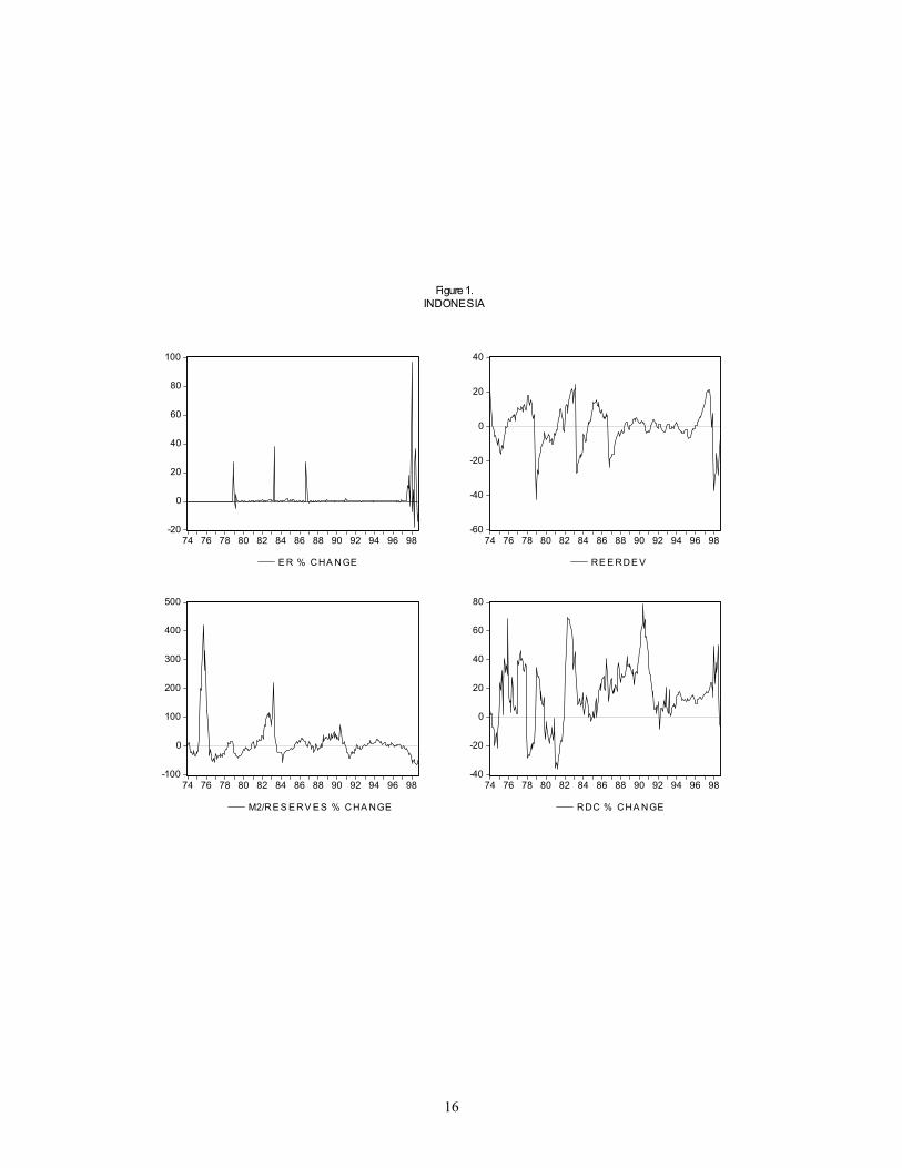
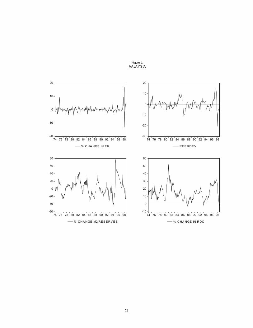
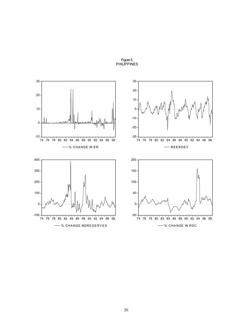
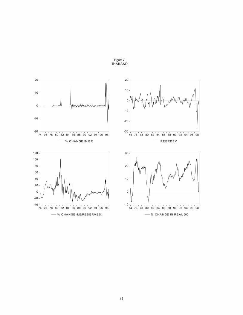
One can then evaluate this at different values of θ to find the maximum likelihood estimate. EMPIRICAL RESULTS Our estimates of univariate Markov switching models for Indonesia, Malaysia, the Philippines, and Thailand, using monthly data from 1974 to 1998, are summarized in the tables in the Appendix. Graphs as well as tabulations of the calculated probabilities of a currency crisis at time t+1 given all information up to time t are obtained from the estimated model and are included as well. Most of the data was sourced from the International Monetary Fund’s International Financial Statistics CD-ROM; real effective exchange rates are from J.P. Morgan. The estimated models are simple mean-switching and variance-switching models of month-to-month percentage changes in nominal exchange rates, with transition probabilities in the Markov chain depending on deviations of real effective exchange rate from trend, year-on-year percentage changes in the ratio of money supply (M2) to gross international reserves, and year-on-year percentage changes in real domestic credit. These are the three variables that the IMF (1998b) found were the best early warning indicators among the dozens of potential candidates. The Hodrick-Prescott filter is used to calculate trends in REER. Graphs of these early warning indicator for the four countries are shown on Figures 1, 3, 5 and 7. The expected signs on the γ coefficients (which determine the probability of staying in state 0) are negative – increases in real overvaluation, growth of real domestic credit and the ratio of M2 to reserves should

7

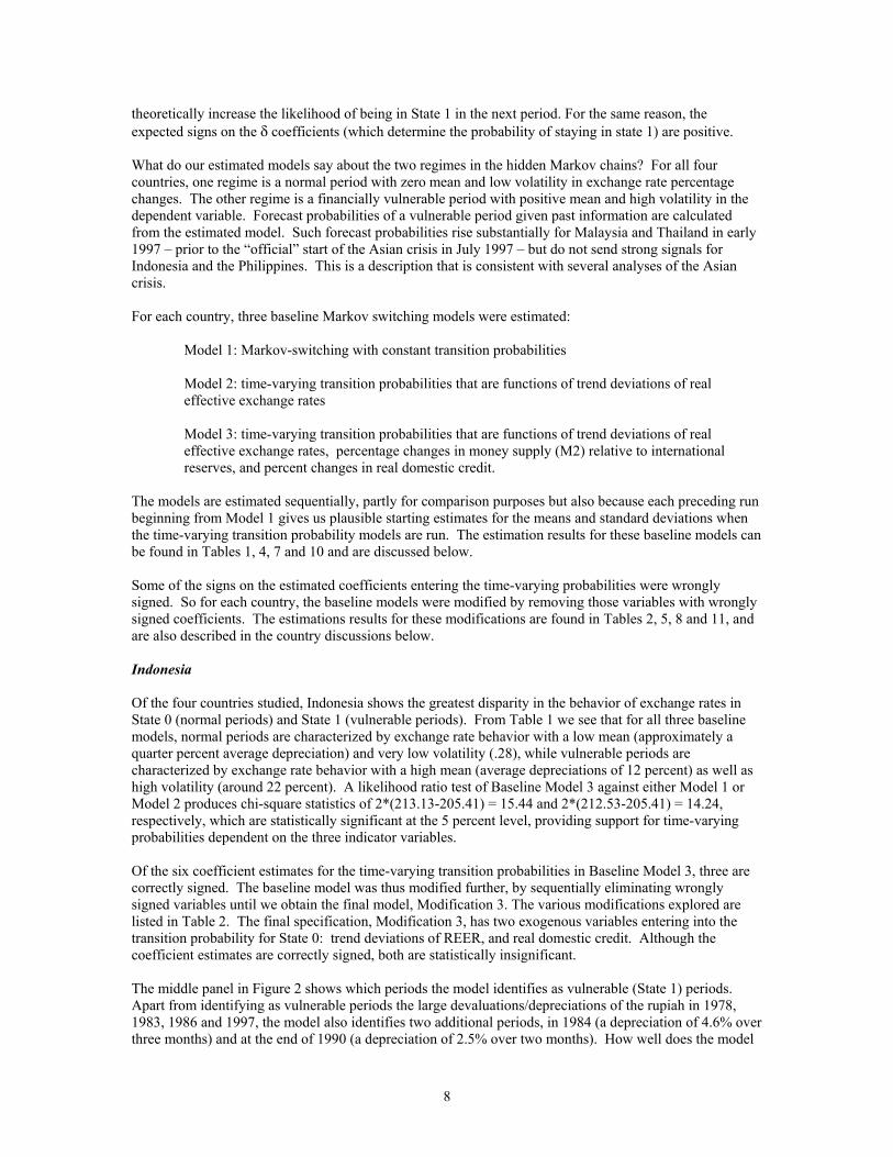
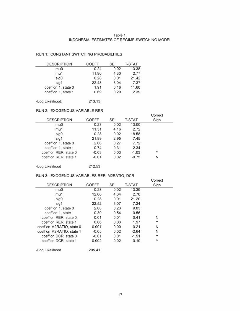
theoretically increase the likelihood of being in State 1 in the next period. For the same reason, the expected signs on the δ coefficients (which determine the probability of staying in state 1) are positive. What do our estimated models say about the two regimes in the hidden Markov chains? For all four countries, one regime is a normal period with zero mean and low volatility in exchange rate percentage changes. The other regime is a financially vulnerable period with positive mean and high volatility in the dependent variable. Forecast probabilities of a vulnerable period given past information are calculated from the estimated model. Such forecast probabilities rise substantially for Malaysia and Thailand in early 1997 – prior to the “official” start of the Asian crisis in July 1997 – but do not send strong signals for Indonesia and the Philippines. This is a description that is consistent with several analyses of the Asian crisis. For each country, three baseline Markov switching models were estimated: Model 1: Markov-switching with constant transition probabilities

Model 2: time-varying transition probabilities that are functions of trend deviations of real effective exchange rates Model 3: time-varying transition probabilities that are functions of trend deviations of real effective exchange rates, percentage changes in money supply (M2) relative to international reserves, and percent changes in real domestic credit.

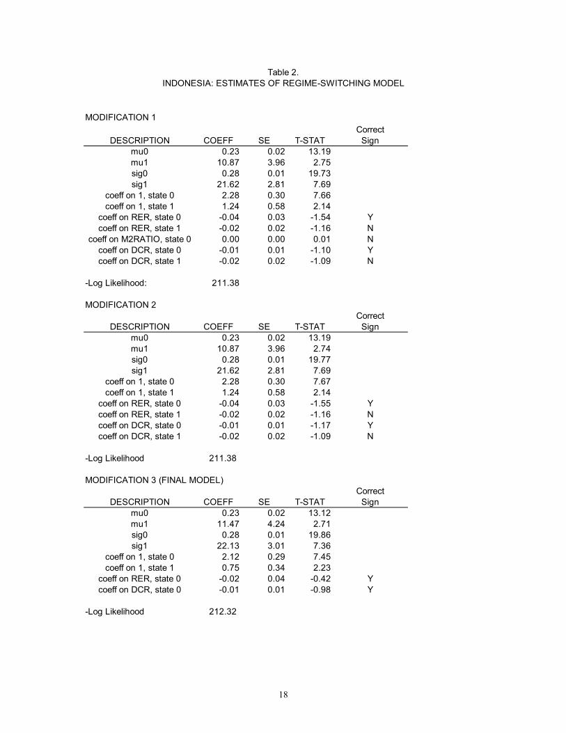
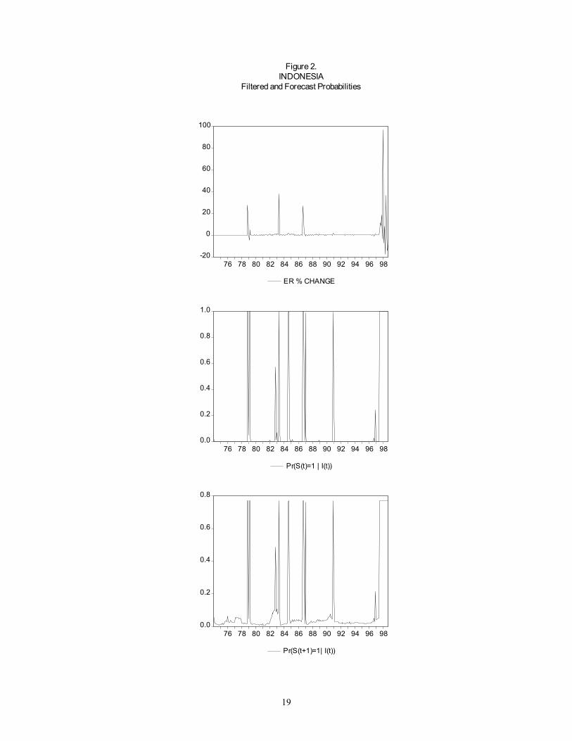
The models are estimated sequentially, partly for comparison purposes but also because each preceding run beginning from Model 1 gives us plausible starting estimates for the means and standard deviations when the time-varying transition probability models are run. The estimation results for these baseline models can be found in Tables 1, 4, 7 and 10 and are discussed below. Some of the signs on the estimated coefficients entering the time-varying probabilities were wrongly signed. So for each country, the baseline models were modified by removing those variables with wrongly signed coefficients. The estimations results for these modifications are found in Tables 2, 5, 8 and 11, and are also described in the country discussions below. Indonesia Of the four countries studied, Indonesia shows the greatest disparity in the behavior of exchange rates in State 0 (normal periods) and State 1 (vulnerable periods). From Table 1 we see that for all three baseline models, normal periods are characterized by exchange rate behavior with a low mean (approximately a quarter percent average depreciation) and very low volatility (.28), while vulnerable periods are characterized by exchange rate behavior with a high mean (average depreciations of 12 percent) as well as high volatility (around 22 percent). A likelihood ratio test of Baseline Model 3 against either Model 1 or Model 2 produces chi-square statistics of 2*(213.13-205.41) = 15.44 and 2*(212.53-205.41) = 14.24, respectively, which are statistically significant at the 5 percent level, providing support for time-varying probabilities dependent on the three indicator variables. Of the six coefficient estimates for the time-varying transition probabilities in Baseline Model 3, three are correctly signed. The baseline model was thus modified further, by sequentially eliminating wrongly signed variables until we obtain the final model, Modification 3. The various modifications explored are listed in Table 2. The final specification, Modification 3, has two exogenous variables entering into the transition probability for State 0: trend deviations of REER, and real domestic credit. Although the coefficient estimates are correctly signed, both are statistically insignificant. The middle panel in Figure 2 shows which periods the model identifies as vulnerable (State 1) periods. Apart from identifying as vulnerable periods the large devaluations/depreciations of the rupiah in 1978, 1983, 1986 and 1997, the model also identifies two additional periods, in 1984 (a depreciation of 4.6% over three months) and at the end of 1990 (a depreciation of 2.5% over two months). How well does the model

8

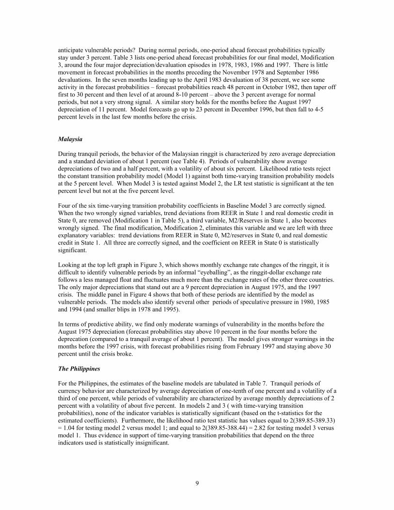
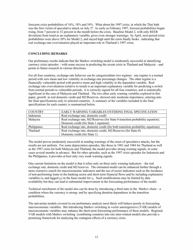
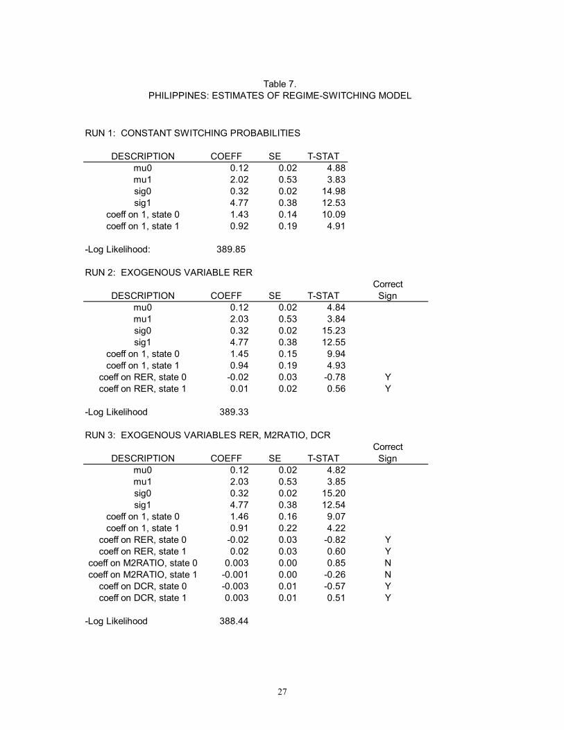
anticipate vulnerable periods? During normal periods, one-period ahead forecast probabilities typically stay under 3 percent. Table 3 lists one-period ahead forecast probabilities for our final model, Modification 3, around the four major depreciation/devaluation episodes in 1978, 1983, 1986 and 1997. There is little movement in forecast probabilities in the months preceding the November 1978 and September 1986 devaluations. In the seven months leading up to the April 1983 devaluation of 38 percent, we see some activity in the forecast probabilities – forecast probabilities reach 48 percent in October 1982, then taper off first to 30 percent and then level of at around 8-10 percent – above the 3 percent average for normal periods, but not a very strong signal. A similar story holds for the months before the August 1997 depreciation of 11 percent. Model forecasts go up to 23 percent in December 1996, but then fall to 4-5 percent levels in the last few months before the crisis. Malaysia During tranquil periods, the behavior of the Malaysian ringgit is characterized by zero average depreciation and a standard deviation of about 1 percent (see Table 4). Periods of vulnerability show average depreciations of two and a half percent, with a volatility of about six percent. Likelihood ratio tests reject the constant transition probability model (Model 1) against both time-varying transition probability models at the 5 percent level. When Model 3 is tested against Model 2, the LR test statistic is significant at the ten percent level but not at the five percent level. Four of the six time-varying transition probability coefficients in Baseline Model 3 are correctly signed. When the two wrongly signed variables, trend deviations from REER in State 1 and real domestic credit in State 0, are removed (Modification 1 in Table 5), a third variable, M2/Reserves in State 1, also becomes wrongly signed. The final modification, Modification 2, eliminates this variable and we are left with three explanatory variables: trend deviations from REER in State 0, M2/reserves in State 0, and real domestic credit in State 1. All three are correctly signed, and the coefficient on REER in State 0 is statistically significant. Looking at the top left graph in Figure 3, which shows monthly exchange rate changes of the ringgit, it is difficult to identify vulnerable periods by an informal “eyeballing”, as the ringgit-dollar exchange rate follows a less managed float and fluctuates much more than the exchange rates of the other three countries. The only major depreciations that stand out are a 9 percent depreciation in August 1975, and the 1997 crisis. The middle panel in Figure 4 shows that both of these periods are identified by the model as vulnerable periods. The models also identify several other periods of speculative pressure in 1980, 1985 and 1994 (and smaller blips in 1978 and 1995). In terms of predictive ability, we find only moderate warnings of vulnerability in the months before the August 1975 depreciation (forecast probabilities stay above 10 percent in the four months before the deprecation (compared to a tranquil average of about 1 percent). The model gives stronger warnings in the months before the 1997 crisis, with forecast probabilities rising from February 1997 and staying above 30 percent until the crisis broke. The Philippines For the Philippines, the estimates of the baseline models are tabulated in Table 7. Tranquil periods of currency behavior are characterized by average depreciation of one-tenth of one percent and a volatility of a third of one percent, while periods of vulnerability are characterized by average monthly depreciations of 2 percent with a volatility of about five percent. In models 2 and 3 ( with time-varying transition probabilities), none of the indicator variables is statistically significant (based on the t-statistics for the estimated coefficients). Furthermore, the likelihood ratio test statistic has values equal to 2(389.85-389.33) = 1.04 for testing model 2 versus model 1; and equal to 2(389.85-388.44) = 2.82 for testing model 3 versus model 1. Thus evidence in support of time-varying transition probabilities that depend on the three indicators used is statistically insignificant.

9

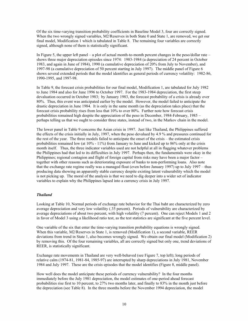
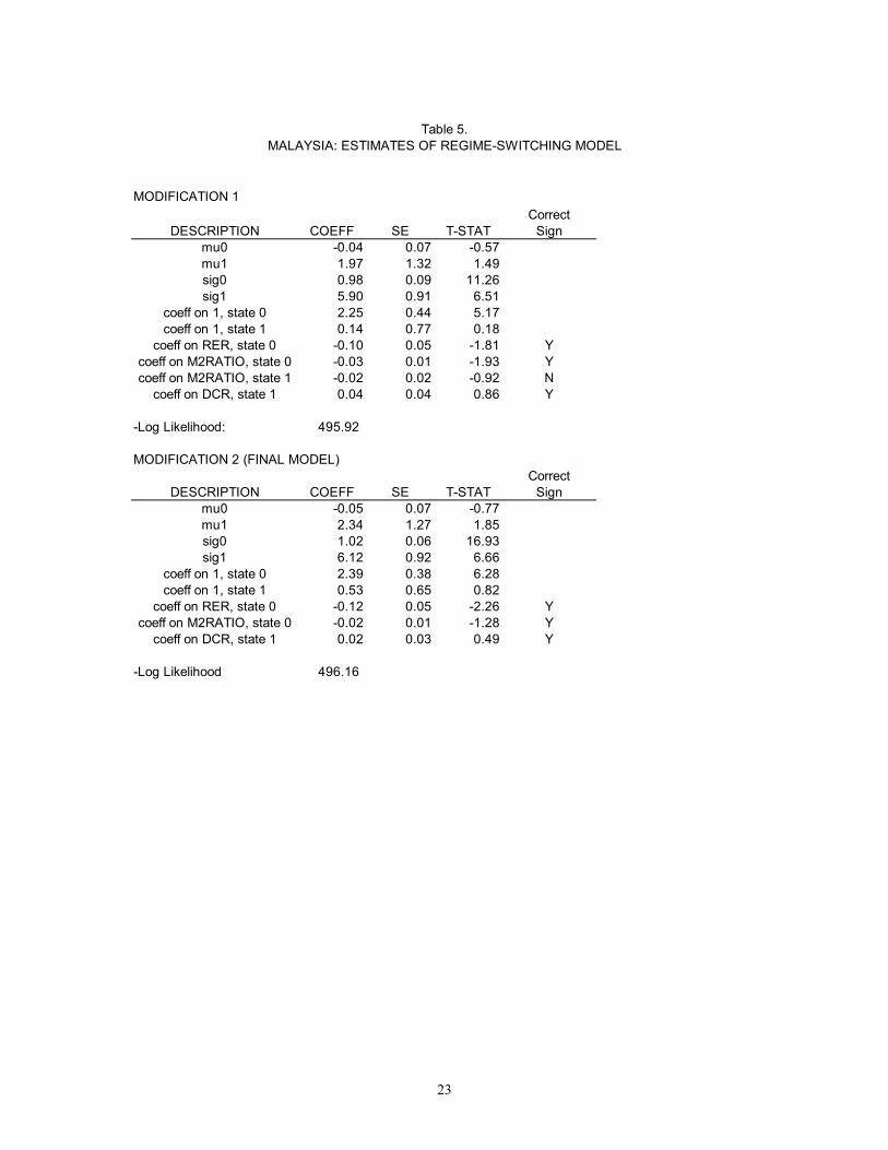
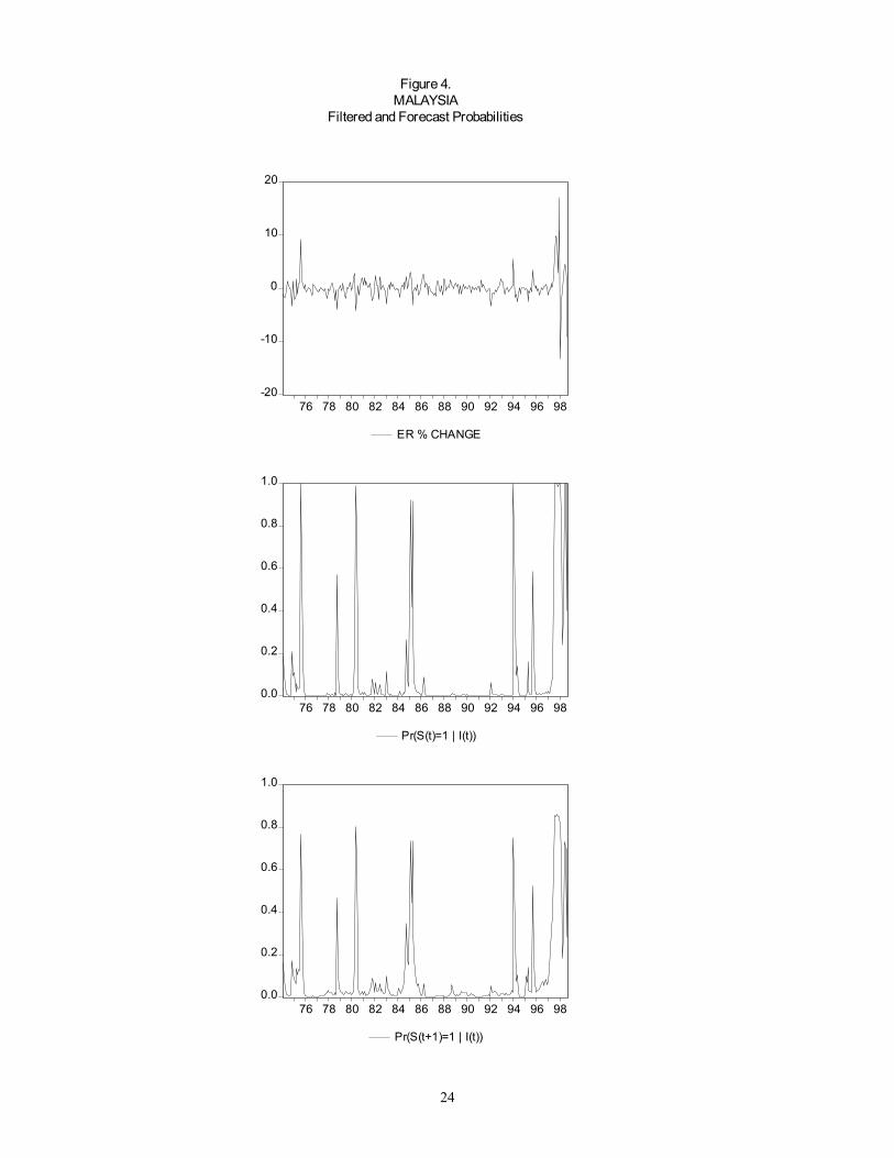
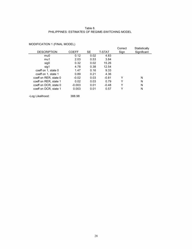
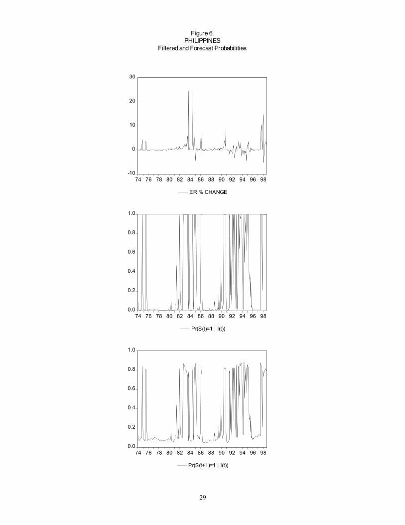
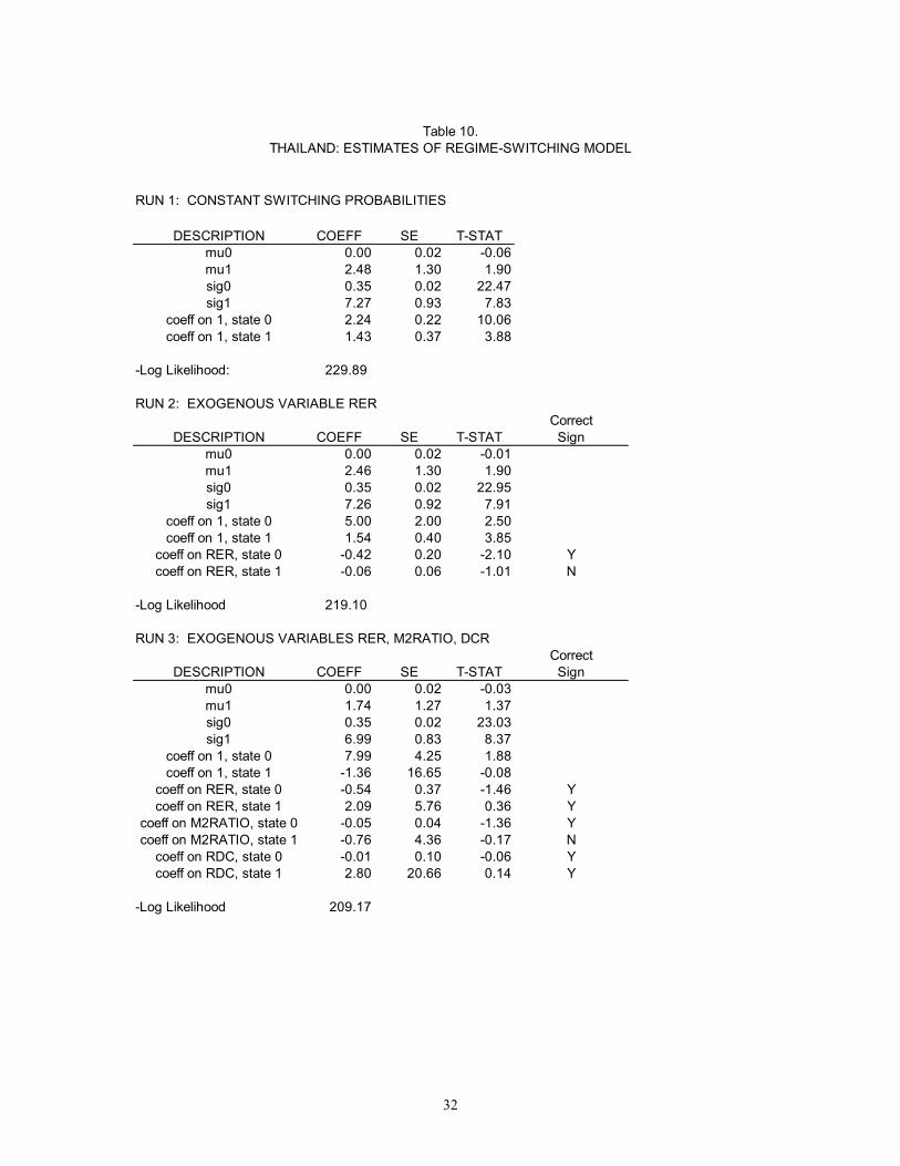
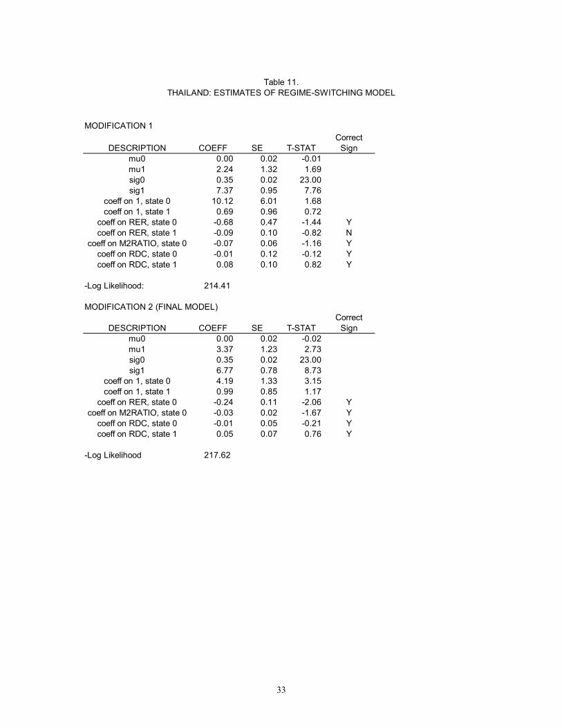
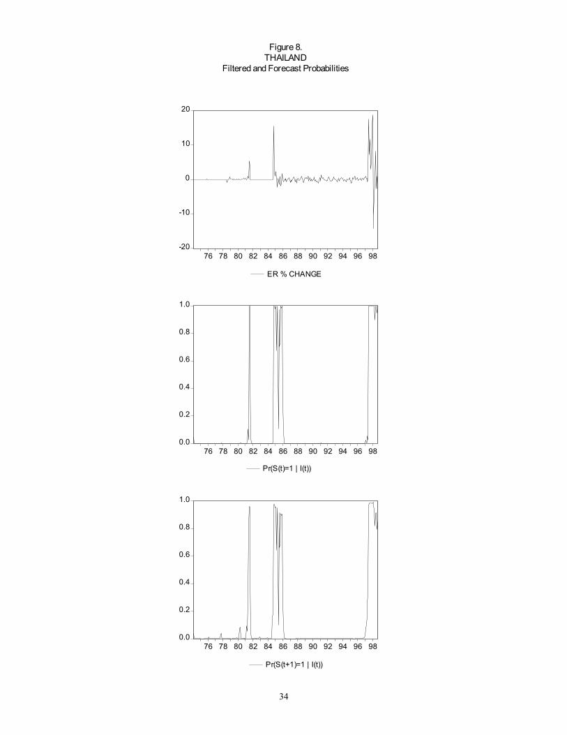
Of the six time-varying transition probability coefficients in Baseline Model 3, four are correctly signed. When the two wrongly signed variables, M2/Reserves in both State 0 and State 1, are removed, we get our final model, Modification 1 which is tabulated in Table 8. The remaining four variables are correctly signed, although none of them is statistically significant. In Figure 5, the upper left panel – a plot of actual month-to-month percent changes in the peso/dollar rate – shows three major depreciation episodes since 1974: 1983-1984 (a depreciation of 24 percent in October 1983, and again in June of 1984), 1990 (a cumulative depreciation of 20% from July to November), and 1997-98 (a cumulative depreciation of 50 percent starting in July 1997). The middle panel of Figure 6 shows several extended periods that the model identifies as general periods of currency volatility: 1982-86, 1990-1995, and 1997-98. In Table 9, the forecast crisis probabilities for our final model, Modification 1, are tabulated for July 1982 to June 1984 and also for June 1996 to October 1997. For the 1983-1984 depreciation, the first steep devaluation occurred in October 1983; by January 1983, the forecast probability of a crisis is already over 80%. Thus, this event was anticipated earlier by the model. However, the model failed to anticipate the drastic depreciation in June 1984. It is only in the same month (as the depreciation takes place) that the forecast crisis probability rises from less that 10% to over 80%. Further note how forecast crisis probabilities remained high despite the appreciation of the peso in December, 1984-February, 1985 – perhaps telling us that we ought to consider three states, instead of two, in the Markov chain in the model. The lower panel in Table 9 concerns the Asian crisis in 1997. Just like Thailand, the Philippines suffered the effects of the crisis initially in July, 1997, when the peso devalued by 4.9 % and pressures continued for the rest of the year. The three models failed to anticipate the onset of the crisis – the estimated crisis probabilities remained low (at 10% - 11%) from January to June and kicked up to 86% only at the crisis month itself. Thus, the three indicator variables used are not helpful at all in flagging whatever problems the Philippines had that led to its difficulties in July 1997. Perhaps then, the fundamentals were okay in the Philippines; regional contagion and flight of foreign capital from risks may have been a major factor – together with other reasons such as deteriorating exposure of banks to non-performing loans. Also note that the exchange rate regime really was a managed float (even before January 1997) up to July 1997 – thus producing data showing an apparently stable currency despite existing latent vulnerability which the model is not picking up. The moral of the analysis is that we need to dig deeper into a wider set of indicator variables to explain why the Philippines lapsed into a currency crisis in July 1997. Thailand Looking at Table 10, Normal periods of exchange rate behavior for the Thai baht are characterized by zero average depreciation and very low volatility (.35 percent). Periods of vulnerability are characterized by average depreciations of about two percent, with high volatility (7 percent). One can reject Models 1 and 2 in favor of Model 3 using a likelihood ratio test, as the test statistics are significant at the five percent level. One variable of the six that enter the time-varying transition probability equations is wrongly signed. When this variable, M2/Reserves in State 1, is removed (Modification 1), a second variable, REER deviations from trend in State 1, also becomes wrongly signed. We obtain our final model (Modification 2) by removing this. Of the four remaining variables, all are correctly signed but only one, trend deviations of REER, is statistically significant. Exchange rate movements in Thailand are very well-behaved (see Figure 7, top left); long periods of relative calm (1974-81, 1981-84, 1985-97) are interrupted by sharp depreciations in July 1981, November 1984 and July 1997. These are the crisis episodes that the model identifies (Figure 8, middle panel). How well does the model anticipate these periods of currency vulnerability? In the four months immediately before the July 1981 depreciation, the model estimates of one-period ahead forecast probabilities rise first to 10 percent, to 27% two months later, and finally to 83% in the month just before the depreciation (see Table 8). In the three months before the November 1994 depreciation, the model

10

forecasts crisis probabilities of 16%, 18% and 54%. What about the 1997 crisis, in which the Thai baht was the first victim of speculative attack on July 2? As early as February 1997, forecast probabilities began rising, from 7 percent to 32 percent in the month before the crisis. Baseline Model 2, with only REER deviations from trend as an explanatory variable, gives even stronger warnings; by April, next-period crisis probabilities were above 50% for Model 2, and stayed high until the crisis finally broke. indicating that real exchange rate overvaluation played an important role in Thailand’s 1997 crisis. CONCLUDING REMARKS Our preliminary results indicate that the Markov switching model is moderately successful at identifying currency crisis episodes – with some success in predicting the recent crisis in Thailand and Malaysia – and points to future research in various directions. For all four countries, exchange rate behavior can be categorizedinto two regimes: one regime is a normal period with zero mean and low volatility in exchange rate percentage changes. The other regime is a financially vulnerable period with positive mean and high volatility in the dependent variable. Real exchange rate overvaluation (relative to trend) is an important explanatory variable for predicting a switch from normal periods to vulnerable periods; it is correctly signed for all four countries, and is statistically significant in the case of Malaysia and Thailand. The two other early warning variables explored in this paper, growth in real domestic credit and M2/Reserves, showed only moderate importance, entering into the final specifications only in selected countries. A summary of the variables included in the final specifications for each country is summarized below. COUNTRY EARLY WARNING VARIABLES ENTERING FINAL SPECIFICATION Indonesia Real exchange rate, domestic credit Malaysia Real exchange rate, M2/Reserves (for State 0 transition probability equation);

Domestic credit (for State 1 equation) Philippines Real exchange rate, domestic credit (for both transition probability equations) Thailand Real exchange rate, domestic credit, M2/Reserves (for State 0)

Domestic credit (for State 1) The model proves moderately successful at sending warnings of the onset of speculative attacks, but the results are not uniform. For some depreciation episodes, like those in 1981 and 1984 for Thailand as well as the 1997 crisis for both Malaysia and Thailand, the model provides strong warning signals, in some cases several months in advance. But for other episodes, such as the 1997 crisis episodes for Indonesia and the Philippines, it provides at best only very weak warning signals. One current limitation on the model is that it relies only on three early warning indicators – the real exchange rate, domestic credit and M2/reserves. The estimated model can be enhanced further through a more extensive search for macroeconomic indicators and the use of sector indicators such as the incidence of non-performing loans in the banking sector and short-term financial flows and by including explanatory variables (xt and lagged yt) in the basic model for yt. Such modifications may be limited by data availability but they can lead to substantial improvement in the forecasting performance of the model. Technical enrichment of the model also can be done by introducing a third state in the Markov chain – a condition where the currency is strong- and by specifying duration dependence in the transition probabilities. The univariate models covered in our preliminary analysis most likely will behave poorly in forecasting macroeconomic variables. But introducing Markov switching in vector autoregressive (VAR) models of macroeconomic variables may enhance the short-term forecasting performance of these models. Regional VAR models with Markov switching (combining countries into one inter-related model) also provide a promising framework for analyzing the contagion effects of a currency crisis.

11

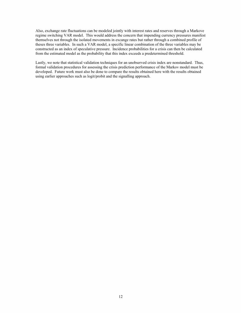
Also, exchange rate fluctuations can be modeled jointly with interest rates and reserves through a Markove regime switching VAR model. This would address the concern that impending currency pressures manifest themselves not through the isolated movements in excange rates but rather through a combined profile of theses three variables. In such a VAR model, a specific linear combination of the three variables may be constructed as an index of speculative pressure. Incidence probabilities for a crisis can then be calculated from the estimated model as the probability that this index exceeds a predetermined threshold. Lastly, we note that statistical validation techniques for an unobserved crisis index are nonstandard. Thus, formal validation procedures for assessing the crisis prediction performance of the Markov model must be developed. Future work must also be done to compare the results obtained here with the results obtained using earlier approaches such as logit/probit and the signalling approach.

12

REFERENCES Abiad, A. G. (2002). Early Warning Systems for Currency Crises: A Markov Switching Approach with Applications to Southeast Asia. Ph.D. dissertation – Department of Economics, University of Pennsylvania. Cerra, V. and Saxena, S. (2000). "Contagion, Monsoons, and Domestic Turmoil in Indonesia: A Case Study in the Asian Currency Crisis" IMF Working Paper, May 2000. Demirguc-Kunt, A. & Detragiache, E. (1998) “The Determinants of Banking Crises in Developing and Developed Countries” IMF Staff Papers, Vol. 45 No. 1, 81-109. Dewachter, H. (2001). "Can Markov Switching Models replicate Chartist Profits in the Foreign Exchnage Market?" Journal of International Money and Finance 20, 25-41. Eichengreen, B. and Rose, A. (1998) “Staying Afloat When the Wind Shifts: External Factors and Emerging-Market Banking Crises” NBER Working Paper No. 6370. Cambridge, Massachusetts. Glick, R. and Moreno, R. (1999). "Money and Credit, Competitiveness, and Currency Crises in Asia and Latin America" Federal Reserve Bank of San Francisco Working Paper PB99-01, March 1999. Gochoco-Bautista, S. M. (2000) "Periods of Currency Pressure: Stylized Facts and Leading Indicators" Journal of Macroeconomics 22. Goldstein, M. G. (1998). The Asian Financial Crisis: Causes, Cures, and Systemic Implications. Institute for International Economics, Washington, D.C. Goldstein, M. G., Kaminsky, G., and Reinhart, C. (2000) Assessing Financial Vulnerability: An Early Warning System for Emerging Markets. Washington, D.C., Institute for International Economics. Gong, F. & Mariano, R. S. (1997) Testing Under Non-standard Conditions in Frequency Domain: With Applications to Markov Regime Switching Models of Exchange Rates and the Federal Funds Rate. Federal Reserve Bank of New York Technical Staff Report. IMF (1998a) International Financial Markets. Washington, D.C. IMF (1998b) World Economic Outlook. Washington, D.C. Kahler, M. (1998, ed). Capital Flows and Financial Crises. Cornell University Press, Ithaca. Kaminsky, G.and Reinhart, C. (1998) “Financial Crises in Asia and Latin America: Then and Now.” American Economic Review 88, 444-448 Kaminsky, G. and Reinhart, C. (1999a) “On crises, contagion, and confusion” Journal of International Economics 51, 145-168. Kaminsky, G. and Reinhart, C. (1999b) “The Twin Crises: The Causes of Banking and Balance of Payments Problems” American Economic Review 89, 473-500. Kaminsky, G., Lizondo, S., and Reinhart, C. (1998) “Leading Indicators of Currency Crises.” IMF Staff Papers. Vol. 45 (1). 1-48. March 1998. Kim, C. J. and C. Nelson (1999) State-Space Models with Regime Switching. MIT Press.

13

Krugman, P. (1979). “A Model of Balance of Payments Crises.” Journal of Money, Credit and Banking, 11, 311-325. Mariano, R. S., Gultekin, B. N., Ozmucur, S. and Shabbir, T. (1999). Predictive Models of Economic Financial Crises (Interim Report). Report submitted to the Economic Research Forum (ERF) for the Arab countries, Iran and Turkey for ERF Research Project ERF99-US-4004. Department of Economics, University of Pennsylvania. Martinez-Peria, M. S.(1999). “A Regime Switching Approach to Studying Speculative Attacks: A Focus on European Monetary System Crises.” World Bank Development Research Group Working Paper 2132, June 1999. Masson, P. (1998). “Contagion: Monsoonal Effects, Spillovers and Jumps between Multiple Equilibria.” IMF Working Paper 98/142. McLeod R. and Garnaut, R. (1998, eds.). East Asia in Crisis. Routledge, New York. Montes, M. (1998). The Currency Crisis in Southeast Asia. Singapore: Institute of Southeast Asian Studies, 1998. Moreno, R. (1995). "Macroeconomic Behavior During Periods of Speculative Pressure or Realignment: Evidence from Pacific-Basin Economies" Federal Reserve Bank of San Francisco Economic Review, 3-16. Obstfeld, M. (1994). “The Logic of Currency Crises.” Cahiers Economiques et Monetaires, 43, 189-213. Richter, F. (2000, ed) The East Asian development Model: Economic Growth, Institutional Failure and the Aftermath of the Crisis. St. Martin's Press, New York. Tan, A. H. H. (1999). "The Asian Economic Crisis: The Way Ahead for Singapore" May, 1999. Tan, A. H. H. (2000). "Sources of the Asian Currency Crisis: Internal & External" ASEAN University Network & The Korean Association of Southeast Asian Studies, 306-316, December, 2000.

14

15

-20

0

20

40

60

80

100

74 76 78 80 82 84 86 88 90 92 94 96 98

E R % CHA NGE

-60

-40

-20

0

20

40

74 76 78 80 82 84 86 88 90 92 94 96 98

RE E RDE V

-100

0

100

200

300

400

500

74 76 78 80 82 84 86 88 90 92 94 96 98

M2/RE S E RV E S % CHA NGE

-40

-20

0

20

40

60

80

74 76 78 80 82 84 86 88 90 92 94 96 98

RDC % CHA NGE

Figure 1.INDONESIA

16

RUN 1: CONSTANT SWITCHING PROBABILITIES

DESCRIPTION COEFF SE T-STATmu0 0.24 0.02 13.38mu1 11.90 4.30 2.77sig0 0.28 0.01 21.42sig1 22.43 3.04 7.37

coeff on 1, state 0 1.91 0.16 11.60coeff on 1, state 1 0.69 0.29 2.39

-Log Likelihood: 213.13

RUN 2: EXOGENOUS VARIABLE RERCorrect

DESCRIPTION COEFF SE T-STAT Signmu0 0.23 0.02 13.00mu1 11.31 4.16 2.72sig0 0.28 0.02 18.58sig1 21.99 2.95 7.45


coeff on RER, state 0 -0.03 0.03 -1.03 Ycoeff on RER, state 1 -0.01 0.02 -0.75 N

-Log Likelihood 212.53

RUN 3: EXOGENOUS VARIABLES RER, M2RATIO, DCRCorrect



coeff on RER, state 0 0.01 0.01 0.41 Ncoeff on RER, state 1 0.06 0.03 1.97 Y

coeff on M2RATIO, state 0 0.001 0.00 0.21 Ncoeff on M2RATIO, state 1 -0.05 0.02 -2.64 N

coeff on DCR, state 0 -0.01 0.01 -1.51 Ycoeff on DCR, state 1 0.002 0.02 0.10 Y


INDONESIA: ESTIMATES OF REGIME-SWITCHING MODELTable 1.

17

MODIFICATION 1Correct




coeff on M2RATIO, state 0 0.00 0.00 0.01 Ncoeff on DCR, state 0 -0.01 0.01 -1.10 Ycoeff on DCR, state 1 -0.02 0.02 -1.09 N





coeff on RER, state 0 -0.04 0.03 -1.55 Ycoeff on RER, state 1 -0.02 0.02 -1.16 Ncoeff on DCR, state 0 -0.01 0.01 -1.17 Ycoeff on DCR, state 1 -0.02 0.02 -1.09 N


MODIFICATION 3 (FINAL MODEL)Correct



coeff on RER, state 0 -0.02 0.04 -0.42 Ycoeff on DCR, state 0 -0.01 0.01 -0.98 Y


Table 2.INDONESIA: ESTIMATES OF REGIME-SWITCHING MODEL

18

-20

0

20

40

60

80

100

76 78 80 82 84 86 88 90 92 94 96 98

ER % CHANGE

0.0

0.2

0.4

0.6

0.8

1.0

76 78 80 82 84 86 88 90 92 94 96 98

Pr(S(t)=1 | I(t))

0.0

0.2

0.4

0.6

0.8

76 78 80 82 84 86 88 90 92 94 96 98

Pr(S(t+1)=1| I(t))

Figure 2.INDONESIA

Filtered and Forecast Probabilities

19

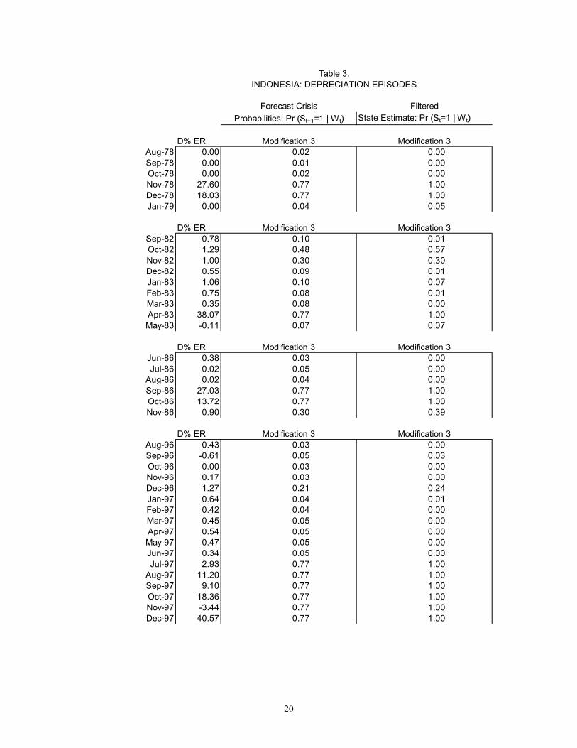
Table 3.INDONESIA: DEPRECIATION EPISODES

Filtered State Estimate: Pr (St=1 | Wt)

D% ER Modification 3 Modification 3Aug-78 0.00 0.02 0.00Sep-78 0.00 0.01 0.00Oct-78 0.00 0.02 0.00Nov-78 27.60 0.77 1.00Dec-78 18.03 0.77 1.00Jan-79 0.00 0.04 0.05

D% ER Modification 3 Modification 3Sep-82 0.78 0.10 0.01Oct-82 1.29 0.48 0.57Nov-82 1.00 0.30 0.30Dec-82 0.55 0.09 0.01Jan-83 1.06 0.10 0.07Feb-83 0.75 0.08 0.01Mar-83 0.35 0.08 0.00Apr-83 38.07 0.77 1.00May-83 -0.11 0.07 0.07

D% ER Modification 3 Modification 3Jun-86 0.38 0.03 0.00Jul-86 0.02 0.05 0.00

Aug-86 0.02 0.04 0.00Sep-86 27.03 0.77 1.00Oct-86 13.72 0.77 1.00Nov-86 0.90 0.30 0.39

D% ER Modification 3 Modification 3Aug-96 0.43 0.03 0.00Sep-96 -0.61 0.05 0.03Oct-96 0.00 0.03 0.00Nov-96 0.17 0.03 0.00Dec-96 1.27 0.21 0.24Jan-97 0.64 0.04 0.01Feb-97 0.42 0.04 0.00Mar-97 0.45 0.05 0.00Apr-97 0.54 0.05 0.00May-97 0.47 0.05 0.00Jun-97 0.34 0.05 0.00Jul-97 2.93 0.77 1.00

Aug-97 11.20 0.77 1.00Sep-97 9.10 0.77 1.00Oct-97 18.36 0.77 1.00Nov-97 -3.44 0.77 1.00Dec-97 40.57 0.77 1.00

Forecast CrisisProbabilities: Pr (St+1=1 | Wt)

20

-20

-10

0

10

20

74 76 78 80 82 84 86 88 90 92 94 96 98

% CHA NGE IN E R

-30

-20

-10

0

10

20

74 76 78 80 82 84 86 88 90 92 94 96 98

RE E RDE V

-60

-40

-20

0

20

40

60

80

74 76 78 80 82 84 86 88 90 92 94 96 98

% CHA NGE M2/RE S E RV E S

-10

0

10

20

30

40

50

60

74 76 78 80 82 84 86 88 90 92 94 96 98

% CHA NGE IN RDC

Figure 3.MALAYSIA

21


DESCRIPTION COEFF SE T-STATmu0 -0.04 0.07 -0.54mu1 1.83 1.24 1.48sig0 0.96 0.10 9.56sig1 5.80 0.98 5.91




DESCRIPTION COEFF SE T-STAT Signmu0 -0.05 0.07 -0.75mu1 2.46 1.30 1.89sig0 1.03 0.05 18.87sig1 6.23 0.95 6.54








coeff on M2RATIO, state 0 -0.03 0.02 -1.73 Ycoeff on M2RATIO, state 1 0.03 0.04 0.70 Y

coeff on DCR, state 0 0.07 0.05 1.32 Ncoeff on DCR, state 1 0.02 0.05 0.39 Y


MALAYSIA: ESTIMATES OF REGIME-SWITCHING MODELTable 4.

22




coeff on RER, state 0 -0.10 0.05 -1.81 Ycoeff on M2RATIO, state 0 -0.03 0.01 -1.93 Ycoeff on M2RATIO, state 1 -0.02 0.02 -0.92 N

coeff on DCR, state 1 0.04 0.04 0.86 Y





coeff on RER, state 0 -0.12 0.05 -2.26 Ycoeff on M2RATIO, state 0 -0.02 0.01 -1.28 Y

coeff on DCR, state 1 0.02 0.03 0.49 Y


MALAYSIA: ESTIMATES OF REGIME-SWITCHING MODELTable 5.

23

-20

-10

0

10

20

76 78 80 82 84 86 88 90 92 94 96 98

ER % CHANGE

0.0

0.2

0.4

0.6

0.8

1.0

76 78 80 82 84 86 88 90 92 94 96 98

Pr(S(t)=1 | I(t))

0.0

0.2

0.4

0.6

0.8

1.0

76 78 80 82 84 86 88 90 92 94 96 98

Pr(S(t+1)=1 | I(t))

Figure 4.MALAYSIA


24

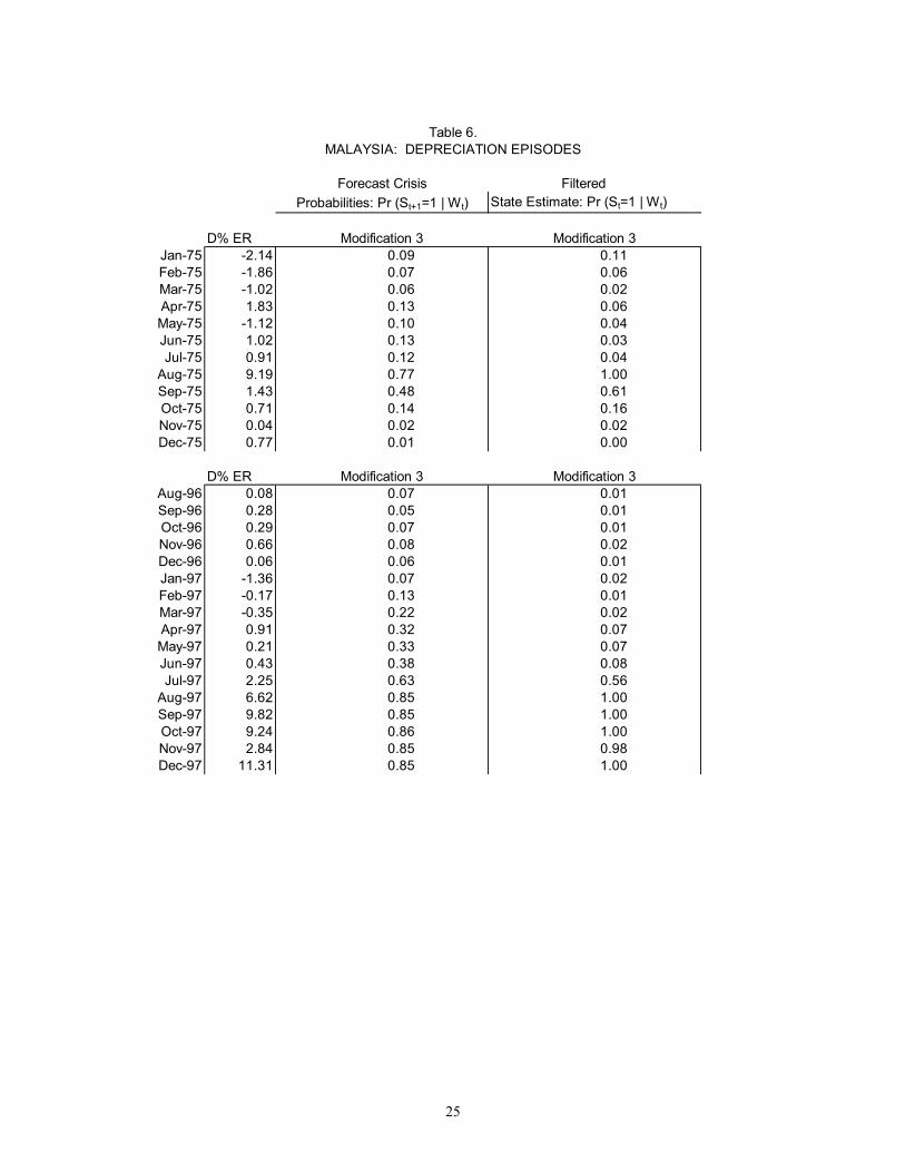
Table 6.MALAYSIA: DEPRECIATION EPISODES


D% ER Modification 3 Modification 3Jan-75 -2.14 0.09 0.11Feb-75 -1.86 0.07 0.06Mar-75 -1.02 0.06 0.02Apr-75 1.83 0.13 0.06May-75 -1.12 0.10 0.04Jun-75 1.02 0.13 0.03Jul-75 0.91 0.12 0.04

Aug-75 9.19 0.77 1.00Sep-75 1.43 0.48 0.61Oct-75 0.71 0.14 0.16Nov-75 0.04 0.02 0.02Dec-75 0.77 0.01 0.00

D% ER Modification 3 Modification 3Aug-96 0.08 0.07 0.01Sep-96 0.28 0.05 0.01Oct-96 0.29 0.07 0.01Nov-96 0.66 0.08 0.02Dec-96 0.06 0.06 0.01Jan-97 -1.36 0.07 0.02Feb-97 -0.17 0.13 0.01Mar-97 -0.35 0.22 0.02Apr-97 0.91 0.32 0.07May-97 0.21 0.33 0.07Jun-97 0.43 0.38 0.08Jul-97 2.25 0.63 0.56


Forecast CrisisProbabilities: Pr (St+1=1 | Wt)

25

-10

0

10

20

30

74 76 78 80 82 84 86 88 90 92 94 96 98

% CHA NGE IN E R

-30

-20

-10

0

10

20

30

74 76 78 80 82 84 86 88 90 92 94 96 98

RE E RDE V

-100

0

100

200

300

400

74 76 78 80 82 84 86 88 90 92 94 96 98

% CHA NGE M2/RE S E RV E S

-50

0

50

100

150

200

74 76 78 80 82 84 86 88 90 92 94 96 98

% CHA NGE IN RDC

Figure 5.PHILIPPINES

26


DESCRIPTION COEFF SE T-STATmu0 0.12 0.02 4.88mu1 2.02 0.53 3.83sig0 0.32 0.02 14.98sig1 4.77 0.38 12.53






coeff on RER, state 0 -0.02 0.03 -0.78 Ycoeff on RER, state 1 0.01 0.02 0.56 Y






coeff on M2RATIO, state 0 0.003 0.00 0.85 Ncoeff on M2RATIO, state 1 -0.001 0.00 -0.26 N

coeff on DCR, state 0 -0.003 0.01 -0.57 Ycoeff on DCR, state 1 0.003 0.01 0.51 Y


Table 7.PHILIPPINES: ESTIMATES OF REGIME-SWITCHING MODEL

27

MODIFICATION 1 (FINAL MODEL)Correct Statistically

DESCRIPTION COEFF SE T-STAT Sign Significantmu0 0.12 0.02 4.83mu1 2.03 0.53 3.84sig0 0.32 0.02 15.26sig1 4.78 0.38 12.54


coeff on RER, state 0 -0.02 0.03 -0.81 Y Ncoeff on RER, state 1 0.02 0.03 0.79 Y Ncoeff on DCR, state 0 -0.003 0.01 -0.48 Y Ncoeff on DCR, state 1 0.003 0.01 0.57 Y N


Table 8.PHILIPPINES: ESTIMATES OF REGIME-SWITCHING MODEL

28

-10

0

10

20

30

74 76 78 80 82 84 86 88 90 92 94 96 98

ER % CHANGE

0.0

0.2

0.4

0.6

0.8

1.0

74 76 78 80 82 84 86 88 90 92 94 96 98

Pr(S(t)=1 | I(t))

0.0

0.2

0.4

0.6

0.8

1.0

74 76 78 80 82 84 86 88 90 92 94 96 98

Pr(S(t+1)=1 | I(t))

Figure 6.PHILIPPINES


29

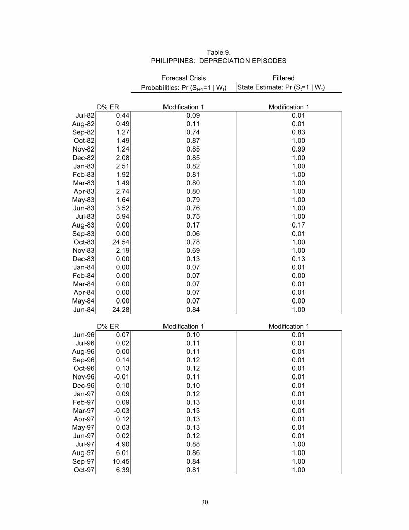
Table 9.PHILIPPINES: DEPRECIATION EPISODES


D% ER Modification 1 Modification 1Jul-82 0.44 0.09 0.01

Aug-82 0.49 0.11 0.01Sep-82 1.27 0.74 0.83Oct-82 1.49 0.87 1.00Nov-82 1.24 0.85 0.99Dec-82 2.08 0.85 1.00Jan-83 2.51 0.82 1.00Feb-83 1.92 0.81 1.00Mar-83 1.49 0.80 1.00Apr-83 2.74 0.80 1.00May-83 1.64 0.79 1.00Jun-83 3.52 0.76 1.00Jul-83 5.94 0.75 1.00

Aug-83 0.00 0.17 0.17Sep-83 0.00 0.06 0.01Oct-83 24.54 0.78 1.00Nov-83 2.19 0.69 1.00Dec-83 0.00 0.13 0.13Jan-84 0.00 0.07 0.01Feb-84 0.00 0.07 0.00Mar-84 0.00 0.07 0.01Apr-84 0.00 0.07 0.01May-84 0.00 0.07 0.00Jun-84 24.28 0.84 1.00

D% ER Modification 1 Modification 1Jun-96 0.07 0.10 0.01Jul-96 0.02 0.11 0.01

Aug-96 0.00 0.11 0.01Sep-96 0.14 0.12 0.01Oct-96 0.13 0.12 0.01Nov-96 -0.01 0.11 0.01Dec-96 0.10 0.10 0.01Jan-97 0.09 0.12 0.01Feb-97 0.09 0.13 0.01Mar-97 -0.03 0.13 0.01Apr-97 0.12 0.13 0.01May-97 0.03 0.13 0.01Jun-97 0.02 0.12 0.01Jul-97 4.90 0.88 1.00

Aug-97 6.01 0.86 1.00Sep-97 10.45 0.84 1.00Oct-97 6.39 0.81 1.00

Probabilities: Pr (St+1=1 | Wt)Forecast Crisis

30

0

-20

-10

10

20

74 76 78 80 82 84 86 88 90 92 94 96 98

% CHA NGE IN E R

-30

-20

-10

0

10

20

74 76 78 80 82 84 86 88 90 92 94 96 98

RE E RDE V

-40

-20

0

20

40

60

80

100

120

74 76 78 80 82 84 86 88 90 92 94 96 98

% CHA NGE (M2/RE S E RV E S )

-10

0

10

20

30

74 76 78 80 82 84 86 88 90 92 94 96 98

% CHA NGE IN RE A L DC

Figure 7.THAILAND

31


DESCRIPTION COEFF SE T-STATmu0 0.00 0.02 -0.06mu1 2.48 1.30 1.90sig0 0.35 0.02 22.47sig1 7.27 0.93 7.83




DESCRIPTION COEFF SE T-STAT Signmu0 0.00 0.02 -0.01mu1 2.46 1.30 1.90sig0 0.35 0.02 22.95sig1 7.26 0.92 7.91






coeff on 1, state 0 7.99 4.25 1.88coeff on 1, state 1 -1.36 16.65 -0.08


coeff on M2RATIO, state 0 -0.05 0.04 -1.36 Ycoeff on M2RATIO, state 1 -0.76 4.36 -0.17 N

coeff on RDC, state 0 -0.01 0.10 -0.06 Ycoeff on RDC, state 1 2.80 20.66 0.14 Y


THAILAND: ESTIMATES OF REGIME-SWITCHING MODELTable 10.

32





coeff on M2RATIO, state 0 -0.07 0.06 -1.16 Ycoeff on RDC, state 0 -0.01 0.12 -0.12 Ycoeff on RDC, state 1 0.08 0.10 0.82 Y





coeff on RER, state 0 -0.24 0.11 -2.06 Ycoeff on M2RATIO, state 0 -0.03 0.02 -1.67 Y

coeff on RDC, state 0 -0.01 0.05 -0.21 Ycoeff on RDC, state 1 0.05 0.07 0.76 Y


THAILAND: ESTIMATES OF REGIME-SWITCHING MODELTable 11.

33

-20

-10

0

10

20

76 78 80 82 84 86 88 90 92 94 96 98

ER % CHANGE

0.0

0.2

0.4

0.6

0.8

1.0

76 78 80 82 84 86 88 90 92 94 96 98

Pr(S(t)=1 | I(t))

0.0

0.2

0.4

0.6

0.8

1.0

76 78 80 82 84 86 88 90 92 94 96 98

Pr(S(t+1)=1 | I(t))

Figure 8.THAILAND


34

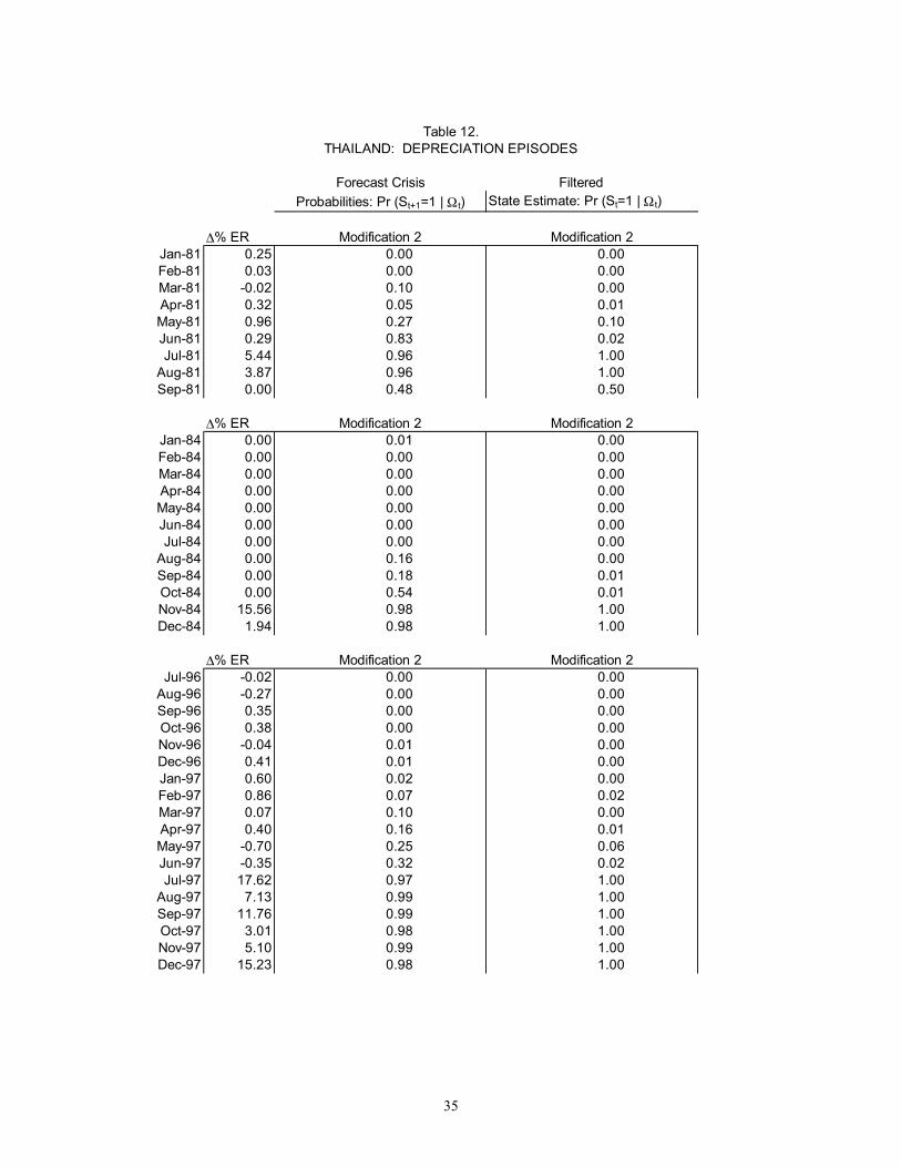
Table 12.THAILAND: DEPRECIATION EPISODES

Filtered State Estimate: Pr (St=1 | Ωt)

∆% ER Modification 2 Modification 2Jan-81 0.25 0.00 0.00Feb-81 0.03 0.00 0.00Mar-81 -0.02 0.10 0.00Apr-81 0.32 0.05 0.01May-81 0.96 0.27 0.10Jun-81 0.29 0.83 0.02Jul-81 5.44 0.96 1.00

Aug-81 3.87 0.96 1.00Sep-81 0.00 0.48 0.50

∆% ER Modification 2 Modification 2Jan-84 0.00 0.01 0.00Feb-84 0.00 0.00 0.00Mar-84 0.00 0.00 0.00Apr-84 0.00 0.00 0.00May-84 0.00 0.00 0.00Jun-84 0.00 0.00 0.00Jul-84 0.00 0.00 0.00


∆% ER Modification 2 Modification 2Jul-96 -0.02 0.00 0.00

Aug-96 -0.27 0.00 0.00Sep-96 0.35 0.00 0.00Oct-96 0.38 0.00 0.00Nov-96 -0.04 0.01 0.00Dec-96 0.41 0.01 0.00Jan-97 0.60 0.02 0.00Feb-97 0.86 0.07 0.02Mar-97 0.07 0.10 0.00Apr-97 0.40 0.16 0.01May-97 -0.70 0.25 0.06Jun-97 -0.35 0.32 0.02Jul-97 17.62 0.97 1.00


Probabilities: Pr (St+1=1 | Ωt)Forecast Crisis

35

Documents

Wharton-SMU Research Center A MARKOV CHAINS IN PREDICTIVE MODELS OF CURRENCY CRISES - WITH APPLICATIONS TO SOUTHEAST ASIA