Embed Size (px)
Citation preview

1 United States Environmental Protection Agency
Office of Water Office of Science and Technology Washington, DC 20460
EPA-823-B-05-003 December 2006 www.epa.gov
2 3 4 5
Draft Nutrient Criteria 6
Technical Guidance Manual7 8 9
10
Wetlands 11 12
13
For assistance in accessing this document pleasesend an email to [email protected]
DRAFT
ii
DISCLAIMER 15 16 17
This manual provides technical guidance to States authorized Tribes, and other authorized 18 jurisdictions to establish water quality criteria and standards under the Clean Water Act (CWA), 19 in order to protect aquatic life from acute and chronic effects of nutrient overenrichment. Under 20 the CWA, States and authorized Tribes are directed to establish water quality criteria to protect 21 designated uses. States and authorized Tribes may use approaches for establishing water quality 22 criteria that differ from the approaches recommended in this guidance. This manual constitutes 23 EPA’s scientific recommendations regarding the development of numeric criteria reflecting 24 ambient concentrations of nutrients that protect aquatic life. However, it does not substitute for 25 the CWA or EPA’s regulations; nor is it a regulation itself. Thus, it cannot impose legally 26 binding requirements on EPA, States, Authorized Tribes, or the regulated community, and might 27 not apply to a particular situation or circumstance. Further, States and Authorized Tribes may 28 choose to develop different types of nutrient criteria for wetlands that are scientifically 29 defensible and protective of the designated use, including narrative criteria. EPA may change 30 this guidance in the future. 31
DRAFT

iii
32 33 34 35 36 37 38 39 40 41 42 43
THIS PAGE INTENTIONALLY 44 LEFT BLANK45
DRAFT

December 2006 DRAFT
iv
TABLE OF CONTENTS 46 47
CONTRIBUTORS.................................................................................................................................................... vii 48 ACKNOWLEDGMENTS....................................................................................................................................... viii 49 LIST OF FIGURES ....................................................................................................................................................ix 50 LIST OF TABLES .......................................................................................................................................................x 51 LIST OF INTERNET LINKS/REFERENCES ........................................................................................................xi 52 EXECUTIVE SUMMARY .........................................................................................................................................1 53 Chapter 1 Introduction .........................................................................................................................................5 54
1.1 INTRODUCTION .........................................................................................................................................5 55 1.2 WATER QUALITY STANDARDS AND CRITERIA ..............................................................................6 56 1.3 NUTRIENT ENRICHMENT PROBLEMS ...............................................................................................8 57 1.4 OVERVIEW OF THE CRITERIA DEVELOPMENT PROCESS........................................................11 58 1.5 ROADMAP TO THE DOCUMENT .........................................................................................................12 59
Chapter 2 Overview of Wetland Science ...........................................................................................................16 60 2.1 INTRODUCTION .......................................................................................................................................16 61 2.2 COMPONENTS OF WETLANDS ............................................................................................................17 62 2.3 WETLAND NUTRIENT COMPONENTS...............................................................................................22 63
Chapter 3 Classification of Wetlands.................................................................................................................30 64 3.1 INTRODUCTION .......................................................................................................................................30 65 3.2 EXISTING WETLAND CLASSIFICATION SCHEMES ......................................................................31 66 3.3 SOURCES OF INFORMATION FOR MAPPING WETLAND CLASSES .........................................42 67 3.4 DIFFERENCES IN NUTRIENT REFERENCE CONDITION OR SENSITIVITY TO NUTRIENTS 68 AMONG WETLAND CLASSES .........................................................................................................................45 69 3.5 RECOMMENDATIONS ............................................................................................................................46 70
Chapter 4 Sampling Design for Wetland Monitoring ......................................................................................50 71 4.1 INTRODUCTION .......................................................................................................................................50 72 4.2 CONSIDERATIONS FOR SAMPLING DESIGN ..................................................................................52 73 4.3 SAMPLING PROTOCOL .........................................................................................................................57 74 4.4 SUMMARY....................................................................................................................................................63 75
Chapter 5 Candidate Variables for Establishing Nutrient Criteria................................................................65 76 5.1 OVERVIEW OF CANDIDATE VARIABLES ........................................................................................65 77 5.2 SUPPORTING VARIABLES ....................................................................................................................67 78 5.3 CAUSAL VARIABLES ..............................................................................................................................70 79 5.4 RESPONSE VARIABLES .........................................................................................................................76 80
Chapter 6 Database Development and New Data Collection...........................................................................82 81 6.1 INTRODUCTION .......................................................................................................................................82 82 6.2 DATABASES AND DATABASE MANAGEMENT ...............................................................................82 83 6.3 QUALITY OF HISTORICAL AND COLLECTED DATA ...................................................................86 84 6.4 COLLECTING NEW DATA .....................................................................................................................88 85 6.5 QUALITY ASSURANCE / QUALITY CONTROL (QA/QC) ...............................................................91 86
Chapter 7 Data Analysis......................................................................................................................................92 87 7.1 INTRODUCTION .......................................................................................................................................92 88 7.2 FACTORS AFFECTING ANALYSIS APPROACH ..............................................................................92 89 7.3 DISTRIBUTION-BASED APPROACHES ..............................................................................................94 90 7.4 RESPONSE-BASED APPROACHES.......................................................................................................95 91 7.5 PARTITIONING EFFECTS AMONG MULTIPLE STRESSORS.......................................................97 92 7.6 STATISTICAL TECHNIQUES....................................................................................................................98 93 7.7 LINKING NUTRIENT AVAILABILITY TO PRIMARY PRODUCER RESPONSE......................101 94
Chapter 8 Criteria Development ......................................................................................................................104 95
DRAFT

December 2006 DRAFT
v
8.1 INTRODUCTION .....................................................................................................................................104 96 8.2 METHODS FOR DEVELOPING NUTRIENT CRITERIA ................................................................105 97 8.4 INTERPRETING AND APPLYING CRITERIA..................................................................................112 98 8.5 SAMPLING FOR COMPARISON TO CRITERIA .............................................................................112 99 8.6 CRITERIA MODIFICATIONS ..............................................................................................................113 100
REFERENCES ........................................................................................................................................................114 101 APPENDIX A. ACRONYM LIST AND GLOSSARY.......................................................................................139 102
ACRONYMS .......................................................................................................................................................139 103 GLOSSARY .........................................................................................................................................................141 104
APPENDIX B. CASE STUDY 1: DERIVING A PHOSPHORUS CRITERION FOR THE FLORIDA 105 EVERGLADES........................................................................................................................................................145 106 APPENDIX B. CASE STUDY 2: THE BENEFICIAL USE OF NUTRIENTS FROM TREATED 107 WASTEWATER EFFLUENT IN LOUISIANA WETLANDS: A REVIEW, ..................................................170 108
DRAFT

vi
109 110 111 112 113 114 115 116 117 118
THIS PAGE INTENTIONALLY 119 LEFT BLANK120
121
DRAFT

December 2006 DRAFT
vii
122 123
CONTRIBUTORS 124 125 126
Nancy Andrews (U.S. Environmental Protection Agency) 127 Mark Clark (University of Florida) 128 Christopher Craft (University of Indiana) 129 William Crumpton (Iowa State University) 130 Ifeyinwa Davis (U.S. Environmental Protection Agency) 131 Naomi Detenbeck (U.S. Environmental Protection Agency) 132 Paul McCormick (U.S. Geological Survey) 133 Amanda Parker (U.S. Environmental Protection Agency)* 134 Kristine Pintado (Louisiana Department of Environmental Quality) 135 Steve Potts (U.S. Environmental Protection Agency) 136 Todd Rasmussen (University of Georgia) 137 Ramesh Reddy (University of Florida) 138 R. Jan Stevenson (Michigan State University) 139 Arnold van der Valk (Iowa State University) 140 141 142 *Principal Author 143
DRAFT
December 2006 DRAFT
viii
144 145
ACKNOWLEDGMENTS 146 147
148 The authors wish to acknowledge the efforts and input of several individuals. These include 149 members of our EPA National Nutrient Team: Jim Carleton, Lisa Larimer and Sharon Frey; 150 members of the EPA Wetlands Division: Kathy Hurld, Chris Faulkner and Donna Downing; and 151 members of the Office of General Counsel: Leslie Darman and Paul Bangser. We also want to 152 thank Kristine Pintado (DEQ, Louisiana) for her contributions and her careful review and 153 comments. 154 155 This document was peer reviewed by a panel of expert scientists. The peer review charge 156 focused on evaluating the scientific validity of the processes and techniques for developing 157 nutrient criteria described in the guidance. The peer review panel comprised Dr. Russel B. 158 Frydenborg, Dr. Robert H. Kadlec, Dr. Lawrence Richards Pomeroy, Dr. Eliska Rejmankova and 159 Dr. Li Zhang. Edits and suggestions made by the peer review panel were incorporated into the 160 final version of the guidance. 161
DRAFT

December 2006 DRAFT
ix
162 LIST OF FIGURES 163
164 Figure 1.1 Flowchart providing the steps of the process to develop wetland nutrient 165 criteria 166 Figure 2.1 Schematic of nutrient transfer among potential system sources and sinks. 167 Figure 2.2 Relationship between water source and wetland vegetation. Modified from 168
Brinson (1993) 169 Figure 2.3 Schematic showing basic nutrient cycles in soil-water column of a wetland 170 Figure 2.4 Range of redox potentials in wetland soils 171 Figure 2.5 Schematic of the nitrogen cycle in wetlands 172 Figure 2.6 Schematic of the phosphorus cycle in wetlands 173 Figure 3.1 Map of Omernik aquatic ecoregions 174 Figure 3.2 Map of Bailey ecoregions with coastal and estuarine provinces 175 Figure 3.3 Examples of first four hierarchical levels of Ecological Units 176 Figure 3.4 Dominant water sources to wetlands, from Brinson 1993 177 Figure 3.5 Dominant hydrodynamic regimes for wetlands based on flow pattern 178 Figure 3.6 Interaction with break in slope with groundwater inputs to slope wetlands 179 Figure 3.7 (Top) Cowardin hierarchy of habitat types for estuarine systems 180 (Bottom) Palustrine systems, from Cowardin et al. 1979 181 Figure 5.1 Conceptual model of causal pathway between human activities and ecological 182
attributes. 183 Figure 7.1 Biological condition gradient model describing biotic community condition as 184
levels of stressors increase. 185 Figure 8.1 Use of undisturbed wetlands as a reference for establishing criteria versus an 186 effects based approach. 187 Figure 8.2 Tiered aquatic life use model used in Maine. 188 Figure 8.3 Percent calcareous algal mat cover in relation to distance from the P source 189 showing the loss of the calcareous algal mat in those sites closer to the source 190 DRAFT

December 2006 DRAFT
x
191 LIST OF TABLES 192
193 Table 1 Observed consequences of cultural eutrophication in freshwater wetlands 194 195 Table 2 Comparison of landscape and wetland classification schemes 196 197 Table 3 Features of the major hydrogeomorphic classes of wetlands that may 198 influence background nutrient concentrations, sensitivity to nutrient loading, 199 nutrient storage forms and assimilative capacity, designated use and choice 200 of endpoints 201 202 Table 4 Comparison of Stratified Probabilistic, Targeted, and BACI Sampling Designs 203
DRAFT

December 2006 DRAFT
xi
204 LIST OF INTERNET LINKS/REFERENCES 205
206 Chapter 1 http://www.epa.gov/waterscience/criteria/nutrient/guidance/index.html 207
http://www.epa.gov/owow/wetlands 208 http://www.epa.gov/waterscience/criteria/nutrient/strategy.html. 209 http://www.epa.gov/owow/wetlands/initiative 210 211 Chapter 2 http://www.arl.noaa.gov/research/programs/airmon.html 212 http://nadp.sws.uiuc.edu/ 213 214 Chapter 3 http://www.epa.gov/emap/remap/index.html 215 http://www.epa.gov/bioindicators/ 216 http://www.epa.gov/waterscience/standards/nutrient.html 217 http://el.erdc.usace.army.mil/wetlands/pdfs/wrpde9.pdf 218 http://water.usgs.gov/GIS/metadata/usgswrd/XML/ecoregion.xml 219 http://www.nwi.fws.gov 220 http://www.wes.army.mil/el/wetlands 221 http://www.epa.gov/waterscience/criteria/wetlands/7Classification.pdf 222 http://www.epa.gov/waterscience/criteria/wetlands/17LandUse.pdf 223 224 Chapter 4 http://www.epa.gov/waterscience/criteria/wetlands/index.html 225 http://www.epa.gov/owow/wetlands/bawwg/case/me.html 226 http://www.epa.gov/owow/wetlands/bawwg/case/mtdev.html 227 http://www.epa.gov/owow/wetlands/bawwg/case/wa.html 228
http://www.epa.gov/owow/wetlands/bawwg/case/fl1.html 229 http://www.epa.gov/owow/wetlands/bawwg/case/fl2.html 230 http://www.epa.gov/owow/wetlands/bawwg/case/oh1.html 231 http://www.epa.gov/owow/wetlands/bawwg/case/mn1.html 232 http://www.epa.gov/owow/wetlands/bawwg/case/or.html 233 http://www.epa.gov/owow/wetlands/bawwg/case/wi1.html 234
235 Chapter 5 http://www.epa.gov/waterscience/criteria/wetlands/10Vegetation.pdf 236 http://www.epa.gov/waterscience/criteria/wetlands/11Algae.pdf 237 http://www.epa.gov/waterscience/criteria/wetlands/9Invertebrate.pdf 238 http://www.epa.gov/waterscience/criteria/wetlands/16Indicators.pdf 239 240 Chapter 6 http://www.nps.ars.usda.gov/programs/nrsas.htm 241 http://www.fs.fed.us/research/ 242 http://www.usbr.gov 243 244 Chapter 7 http://el.erdc.usace.army.mil/wrap/wrap.html 245
http://firehole.humboldt.edu/wetland/twdb.html 246
DRAFT

December 2006 DRAFT
xii
http://www.socialresearchmethods.net/ 247 http://www.math.yorku.ca/SCS/ 248 http://calculators.stat.ucla.edu/powercalc/ 249 http://www.surveysystem.com/sscalc.htm 250 http://www.health.ucalgary.ca/~rollin/stats/ssize/index.html 251 http://www.stat.ohio-state.edu/~jch/ssinput.html 252 http://www.stat.uiowa.edu 253 http://www.epa.gov/waterscience/criteria/wetlands 254 255
Chapter 8 http://www.epa.gov/waterscience/biocriteria/modules/wet101-05-alus-256 monitoring.pdf 257
http://www.epa.gov/owow 258 http://www.wetlandbiogeochemistry.lsu.edu/ 259 http://data.lca.gov/Ivan6/app/app_c_ch9.pdf 260
DRAFT

December 2006 DRAFT Executive Summary
1
261 262
EXECUTIVE SUMMARY 263 264
The purpose of this document is to provide scientifically defensible guidance to assist States, 265 Tribes, and Territories in assessing the nutrient status of their wetlands, and to provide technical 266 assistance for developing regionally-based numeric nutrient criteria for wetland systems. The 267 development of nutrient criteria is part of an initiative by the US Environmental Protection 268 Agency (USEPA) to address the problem of cultural eutrophication, i.e., excess nutrients caused 269 by human activities (USEPA 1998a). Cultural eutrophication is not new; however, traditional 270 efforts at nutrient control have been only moderately successful. Specifically, efforts to control 271 nutrients in water bodies that have multiple nutrient sources (point and nonpoint sources) have 272 been less effective in providing satisfactory, timely remedies for enrichment-related problems. 273 The development of numeric criteria should aid control efforts by providing clear numeric goals 274 for nutrient concentrations. Furthermore, numeric nutrient criteria provide specific water quality 275 goals that will assist researchers in designing improved best management practices. 276 277
In 1998, the USEPA published a report entitled National Strategy for the Development of 278 Regional Nutrient Criteria (USEPA 1998a). This report outlines a framework for development 279 of waterbody-specific technical guidance that can be used to assess nutrient status and develop 280 region-specific numeric nutrient criteria. The document presented here is the wetland-specific 281 technical guidance for developing numeric nutrient criteria. The Nutrient Criteria Technical 282 Guidance Manuals for Rivers and Streams (USEPA, 2000b), Lakes and Reservoirs (USEPA, 283 2000a) and Estuarine and Coastal Marine Waters (USEPA, 2001) have been completed and are 284 available at: http://www.epa.gov/waterscience/criteria/nutrient/guidance/index.html. 285
Section 303(c) of the Clean Water Act directs states to adopt water quality standards for 286 interstate and intrastate waters that are “waters of the United States”. Wetlands are 287 included in the definition of “waters of the United States” (40 C.F.R. 230.2(s)). States 288 should therefore have water quality criteria to protect the designated uses of wetlands that 289 are waters of the U.S. in addition to other surface water types (lakes, streams, estuaries) 290 that have traditionally been monitored and regulated for water quality. This guidance is to 291 assist states in developing numeric nutrient criteria for wetlands, should the State or 292 Autorized Tribe choose to do so. Further, States and Authorized Tribes may choose to 293 develop different types of criteria for wetlands protection, including narrative criteria. 294 295 In this document, the term waterbody is used generically to encompass a wide range of aquatic 296 habitats, from lentic and lotic systems with permanent standing water to wetland systems that 297 have saturated sediments but no standing water, or which are flooded only temporarily. EPA 298 recommends that States, Territories and Tribes' include wetlands in the water quality standards 299 definition of "State waters" by adopting a regulatory definition of "State waters" at least as 300 inclusive as the Federal definition of "waters of the U.S.", and adopting an appropriate definition 301 for “wetlands”. 302
DRAFT

December 2006 DRAFT Executive Summary
2
303 CLASSIFICATION OF WETLANDS 304 305 Classification strategies for nutrient criteria development include: 306
physiographic regions 307
hydrogeomorphic class 308
water depth and duration 309
vegetation type or zone 310
Choosing a specific classification scheme will likely depend on practical considerations, such as: 311 whether a classification scheme is available in mapped digital form or can be readily derived 312 from existing map layers; whether a hydrogeomorphic or other classification scheme has been 313 refined for a particular region and wetland type; and whether classification schemes are already 314 in use for monitoring and assessment of other waterbody types in a state or region. 315 316 SAMPLING DESIGN 317 318 Three sampling designs for new wetland monitoring programs are described: 319
probabilistic sampling 320
targeted/tiered approach 321
BACI (Before/After, Control/Impact) 322
These approaches are designed to obtain a significant amount of information for statistical 323 analyses with relatively minimal effort. Sampling efforts should be designed to collect 324 information that will answer management questions in a way that will allow robust statistical 325 analysis. In addition, site selection, characterization of reference sites or systems, and 326 identification of appropriate index periods are all of particular concern when selecting an 327 appropriate sampling design. Careful selection of sampling design will allow the best use of 328 financial resources and will result in the collection of high quality data for evaluation of the 329 wetland resources of a State or Tribe. 330 331 CANDIDATE VARIABLES FOR ESTABLISHING NUTRIENT CRITERIA 332 333 Candidate variables to use in determining nutrient condition of wetlands and to help identify 334 appropriate nutrient criteria for wetlands consist of supporting variables, causal variables, and 335 response variables. Supporting variables provide information useful in normalizing causal and 336 response variables and categorizing wetlands. Causal variables are intended to characterize 337 nutrient availability (or assimilation) in wetlands and could include nutrient loading rates and 338 soil nutrient concentrations. Response variables are intended to characterize biotic response and 339
DRAFT
December 2006 DRAFT Executive Summary
3
could include community structure and composition of macrophytes and algae. Recommended 340 variables for wetland nutrient criteria development described in this chapter are: 341
1. Causal variables - nutrient loading rates, land use, extractable and total soil nitrogen (N) and 342 phosphorus (P), water column N and P; 343
2. Response variables - nutrient content of wetland vegetation (algal and/or higher plants), 344 aboveground biomass and stem height, macrophyte, algal, and macroinvertebrate community 345 structure and composition; 346
3. Supporting variables - hydrologic condition/balance, conductivity, soil pH, soil bulk density, 347 particle size distribution, soil organic matter content. 348
DATABASE DEVELOPMENT AND NEW DATA COLLECTION 349
A database of relevant water quality information can be an invaluable tool to States and Tribes as 350 they develop nutrient criteria. In some cases existing data are available and can provide 351 additional information that is specific to the region where criteria are to be set. However, little or 352 no data are available for most regions or parameters, and creating a database of newly gathered 353 data is strongly recommended. In the case of existing data, the data should be geolocated, and 354 their suitability (type and quality and sufficient associated metadata) ascertained. 355
DATA ANALYSIS 356
Data analysis is critical to nutrient criteria development. Proper analysis and interpretation of 357 data determine the scientific defensibility and effectiveness of the criteria. Therefore, it is 358 important to evaluate short and long-term goals for wetlands of a given class within the region of 359 concern. The purpose of this chapter is to explore methods for analyzing data that can be used to 360 develop nutrient criteria consistent with these goals. Techniques discussed in this chapter 361 include: 362
Distribution based approaches that examine distributions of primary and supporting 363 variables (i.e., the percentile approach); 364
Response based approaches that develop relationships between measurements of nutrient 365 exposure and ecological responses (i.e., tiered aquatic life uses); 366
Partitioning effects of multiple stressors; 367
Statistical techniques; 368
Multi-metric indices; 369
Linking nutrient availability to primary producer response. 370
371 CRITERIA DEVELOPMENT 372
DRAFT

December 2006 DRAFT Executive Summary
4
373 Several methods can be used to develop numeric nutrient criteria for wetlands; they include, but 374 are not limited to, criteria development methods that are detailed in this document: 375 376
Comparing conditions in known reference systems for each established 377 wetland type and class based on using best professional judgment (BPJ) or 378 identifying reference conditions using frequency distributions of empirical 379 data and identifying criteria using percentile selections of data plotted as 380 frequency distributions. 381
Refining classification systems, using models, and/or examining system 382 biological attributes in comparison to known reference conditions to 383 assess the relationships among nutrients, vegetation or algae, soil, and 384 other variables and identifying criteria based on thresholds where those 385 response relationships change. 386
Using or modifying published nutrient and vegetation, algal, and soil 387 relationships and values to identify appropriate criteria. 388
389 A weight of evidence approach with multiple attributes that combine one or more of the 390 development approaches will produce criteria of greater scientific validity. 391 392 Once criteria are developed, they should be implemented into state water quality programs to be 393 effective. The implementation procedures, particularly for wetland systems, may be complex and 394 will likely vary greatly from state to state. The purpose of this document is to provide guidance 395 on developing numeric nutrient criteria in a scientifically valid manner, and is not intended to 396 address the multiple, complex issues surrounding implementation of water quality criteria and 397 standards. Implementation will be addressed in a different process and additional implementation 398 assistance will also be provided through other technical assistance projects provided by EPA. 399 For issues specific to constructed wetlands, States and Tribes should refer to 400 http://www.epa.gov/owow/wetlands/watersheds/cwetlands.html.401 DRAFT
December 2006 DRAFT Chapter 1. Introduction
5
Chapter 1 Introduction 402 403 1.1 INTRODUCTION 404
405 PURPOSE 406 407 The purpose of this document is to provide technical guidance to assist States and Tribes in 408 assessing the nutrient status of their wetlands by considering water, vegetation and soil 409 conditions, and to provide technical assistance for developing regionally-based, scientifically 410 defensible, numeric nutrient criteria for wetland systems. 411 412 EPA’s development of recommended nutrient criteria is part of an initiative by the US 413 Environmental Protection Agency (USEPA) to address the problem of cultural eutrophication. In 414 1998, the EPA published a report entitled National Strategy for the Development of Regional 415 Nutrient Criteria (USEPA 1998a). The report outlines a framework for development of 416 waterbody-specific technical guidance that can be used to assess nutrient status and develop 417 region-specific numeric nutrient criteria. This document is the technical guidance for developing 418 numeric nutrient criteria for wetlands. Additional more specific information on sampling 419 wetlands is available at: http://www.epa.gov/waterscience/criteria/nutrient/guidance/. 420 421 422 AUTHORITY 423 424 Section 303(c) of the Clean Water Act directs states to adopt water quality standards for 425 interstate and intrastate waters that are “waters of the United States”. Wetlands are 426 included in the definition of “waters of the United States” (40 C.F.R. 230.2(s)). 427 428 In this document, the term waterbody is used generically to encompass a wide range of aquatic 429 habitats, from lentic and lotic systems with permanent standing water to wetland systems that 430 have saturated sediments but no standing water, or which are flooded only temporarily. Wetlands 431 must be legally included in the scope of States’ and Tribes' water quality standards programs for 432 water quality standards to be applicable to wetlands. EPA recommends that States and Tribes 433 include wetlands in the water quality standards definition of "State waters" by adopting a 434 regulatory definition of "State waters" at least as inclusive as the Federal definition of "waters of 435 the U.S.", and adopting an appropriate definition for "wetlands". Examples of different state 436 approaches can be found at: http://www.epa.gov/owow/wetlands/initiatives/. 437 438 Discussions about water quality in this document refer to wetland systems as waters of the US 439 under the authority given to the USEPA in the CWA. EPA recognizes that wetland systems are 440 different from the other waters of the US in that they frequently do not have standing or flowing 441 water, and that the soils and vegetation components are more dominant in these systems than in 442 the other waterbody types (lakes, streams, estuaries). 443
DRAFT
December 2006 DRAFT Chapter 1. Introduction
6
444 BACKGROUND 445 446 Cultural eutrophication (human-caused inputs of excess nutrients in waterbodies) is one of the 447 primary factors resulting in impairment of surface waters in the US (USEPA 1998a). Both point 448 and nonpoint sources of nutrients contribute to impairment of water quality. Point source 449 discharges of nutrients are relatively constant and are controlled by the National Pollutant 450 Discharge Elimination System (NPDES) permitting program. Nonpoint pollutant inputs have 451 increased in recent decades resulting in degraded water quality in many aquatic systems. 452 Nonpoint sources of nutrients are most commonly intermittent and are usually linked to runoff, 453 atmospheric deposition, seasonal agricultural activity, and other irregularly occurring events 454 such as silvicultural activities. Control of nonpoint source pollutants typically focuses on land 455 management activities and regulation of pollutants released to the atmosphere. 456 457 The term eutrophication was coined in reference to lake systems. The use of the term for other 458 waterbody types can be problematic due to the confounding nature of hydrodynamics, light, and 459 other waterbody type differences on the responses of algae and vegetation. Eutrophication in this 460 document refers to human-caused inputs of excess nutrients and is not intended to indicate the 461 same scale or responses to eutrophication found in lake systems and codified in the trophic state 462 index for lakes (Carlson 1977). This manual is intended to provide guidance for identifying 463 deviance from natural conditions with respect to cultural eutrophication in wetland systems. 464 Hydrologic alteration and pollutants other than excess nutrients may amplify or reduce the 465 effects of nutrient pollution, making specific responses to nutrient pollution difficult to quantify. 466 EPA recognizes these issues, and presents recommendations for analyzing wetland systems with 467 respect to nutrient condition for development of nutrient criteria in spite of these confounding 468 factors. 469 470 Cultural eutrophication is not new; however, traditional efforts at nutrient control have been only 471 moderately successful. Specifically, efforts to control nutrients in waterbodies that have multiple 472 nutrient sources (point and nonpoint sources) have been less effective in providing satisfactory, 473 timely remedies for enrichment-related problems. The development of numeric criteria should 474 aid control efforts by providing clear numeric goals for nutrient concentrations. Furthermore, 475 numeric nutrient criteria provide specific water quality goals that will assist researchers in 476 designing improved best management practices. 477 478 479 1.2 WATER QUALITY STANDARDS AND CRITERIA 480
481 States, Territories, and authorized Tribes are responsible for setting water quality standards to 482 protect the physical, biological, and chemical integrity of their waters. “Water quality standards 483 (WQS) are provisions of State or Federal law which consist of a designated use or uses for the 484 waters of the United States and water quality criteria for such waters to protect such uses. Water 485
DRAFT
December 2006 DRAFT Chapter 1. Introduction
7
quality standards are to protect public health or welfare, enhance the quality of the water, and 486 serve the purposes of the Act (40 CFR 131.3)” (USEPA 1994). A water quality standard defines 487 the goals for a waterbody by: 1) designating its specific uses, 2) setting criteria to protect those 488 uses, and 3) establishing an antidegradation policy to protect existing water quality. 489 490 Water quality criteria may be expressed as numeric or narrative criteria. Most of the Nation’s 491 waterbodies do not have numeric nutrient criteria, but instead rely on narrative criteria that 492 describe the desired condition. Narrative criteria are descriptions of conditions necessary for the 493 waterbody to attain its designated. An example of a narrative criterion from Florida is shown 494 below: 495 496 In no case shall nutrient concentrations of a body of water be altered so as to cause 497
an imbalance in natural populations of aquatic flora or fauna. 498 499 Numeric criteria, on the other hand, identify specific values designed to protect specified 500 designated uses such as an aquatic life use. Numeric criteria are values assigned to measurable 501 components of water quality, such as the concentration of a specific constituent that is present in 502 the water column. An example of a numeric criterion is shown below: 503 504
The three month or greater geometric mean of water column total phosphorus [TP] 505 in the Everglades shall not exceed 10 μg/L. 506
507 In addition to narrative and numeric criteria, some States and Tribes use numeric translator 508 mechanisms—mechanisms that translate narrative (qualitative) standards into numeric 509 (quantitative) values for use in evaluating water quality data--as an intermediate step between 510 numeric criteria and water quality standards that are not written into State or Tribal laws but are 511 used internally by the State or Tribal agency as goals and assessment levels for management 512 purposes. 513 514 Numeric criteria provide distinct interpretations of acceptable and unacceptable conditions, form 515 the foundation for measurement of environmental quality, and reduce ambiguity for management 516 and enforcement decisions. The lack of numeric nutrient criteria for most of the Nation’s 517 waterbodies makes it difficult to assess the condition of waters of the US, and to develop 518 protective water quality standards, thus hampering the water quality manager’s ability to protect 519 and improve water quality. 520 521 Many States, Tribes, and Territories have adopted some form of nutrient criteria for surface 522 waters related to maintaining natural conditions and avoiding nutrient enrichment. Most States 523 and Tribes with nutrient criteria in their water quality standards have broad narrative criteria for 524 most waterbodies and may also have site-specific numeric criteria for certain waters of the State. 525 Established criteria most commonly pertain to P concentrations in lakes. Nitrogen criteria, where 526 they have been established, are usually protective of human health effects or relate to toxic 527 effects of ammonia and nitrates. In general, levels of nitrate (10 ppm [mg/L] for drinking water) 528
DRAFT

December 2006 DRAFT Chapter 1. Introduction
8
and ammonia high enough to be problematic for human health or toxic to aquatic life (1.24 mg 529 N/L at pH = 8 and 25°C) will also cause problems of enhanced algal growth (USEPA 1986). 530 531 Numeric nutrient criteria can provide a variety of benefits and may be used in conjunction with 532 State/Tribal and Federal biological assessments, Nonpoint Source Programs, Watershed 533 Implementation Plans, and in development of Total Maximum Daily Loads (TMDLs) to improve 534 resource management and support watershed protection activities at local, State, Tribal, and 535 national levels. Information obtained from compiling existing data and conducting new surveys 536 can provide water quality managers and the public a better perspective on the condition of State, 537 Territorial, and Tribal waters. The compiled waterbody information can be used to most 538 effectively budget personnel and financial resources for the protection and restoration of State 539 waters. In a similar manner, data collected in the criteria development and implementation 540 process can be compared before, during, and after specific management actions. Analyses of 541 these data can determine the response of the waterbody and the effectiveness of management 542 endeavors. 543 544 545 1.3 NUTRIENT ENRICHMENT PROBLEMS 546
547 Water quality can be affected when watersheds are modified by alterations in vegetation, 548 sediment transport, fertilizer use, industrialization, urbanization, or conversion of native forests 549 and grasslands to agriculture and silviculture (Turner and Rabalais 1991; Vitousek et al. 1997; 550 Carpenter et al. 1998). Cultural eutrophication, one of the primary factors resulting in 551 impairment of U. S. surface waters (USEPA 1998a) results from point and nonpoint nutrient 552 sources. Nonpoint pollutant inputs have increased in recent decades and have degraded water 553 quality in many aquatic systems (Carpenter et al. 1998). Control of nonpoint source pollutants 554 focuses on land management activities and regulation of pollutants released to the atmosphere 555 (Carpenter et al. 1998). 556 557 Nutrient enrichment frequently ranks as one of the top causes of water resource impairment. The 558 USEPA reported to Congress that of the waterbodies surveyed and reported impaired, 20 percent 559 of rivers and 50 percent of lakes were listed with nutrients as the primary cause of impairment 560 (USEPA 2000c). Few States or Tribes currently include wetland monitoring in their routine 561 water quality monitoring programs (only eleven States and Tribes reported attainment of 562 designated uses for wetlands in the National Water Quality Inventory 1998 Report to Congress 563 (USEPA 1998b) and only three states used monitoring data as a basis for determining attainment 564 of water quality standards for wetlands); thus, the extent of nutrient enrichment and impairment 565 of wetland systems is largely undocumented. Increased wetland monitoring by States and Tribes 566 will help define the extent of nutrient enrichment problems in wetland systems. 567 568 The best-documented case of cultural eutrophication in wetlands is the Everglades ecosystem. 569 The Everglades ecosystem is a wetland mosaic that is primarily of oligotrophic freshwater 570
DRAFT
December 2006 DRAFT Chapter 1. Introduction
9
marsh. Historically, the greater Everglades ecosystem included vast acreage of freshwater marsh, 571 stands of custard apple, and some cattail south of Lake Okeechobee and Big Cypress Swamp, 572 that eventually drained into Florida Bay. Lake Okeechobee was diked to reduce flooding. The 573 area directly south of Lake Okeechobee was then converted into agricultural lands for cattle 574 grazing and row crop production. The cultivation and use of commercial fertilizers in the area 575 now known as the “Everglades Agricultural Area” has resulted in release of nutrient-rich waters 576 into the Everglades for more than thirty years. The effects of the nutrient-rich water, combined 577 with coastal development and channeling water to supply water to communities on the southern 578 Florida coast have resulted in significant increases in soil and water column phosphorus levels in 579 naturally oligotrophic areas. In particular, nutrient enrichment of the freshwater marsh has 580 resulted in an imbalance in the native vegetation. Cattail is now encroaching in areas that were 581 historically primarily sawgrass; calcareous algal mats are being replaced by non-calcareous 582 algae, changing the balance of native flora that is needed to support vast quantities of wildlife. 583 Nutrient enriched water is also reaching Florida Bay, suffocating the native turtle grass as 584 periphyton covers the blades (Davis and Ogden 1994; Everglades Interim Report 1999, 2003; 585 Everglades Consolidated Report 2003). Current efforts to restore the Everglades are focusing on 586 nutrient reduction and better hydrologic management (Everglades Consolidated Report 2003). 587 588 Monitoring to establish trends in nutrient levels and associated changes in biology has been 589 infrequent for most wetland types as compared to studies in the Everglades or examination of 590 other surface waters such as lakes. Noe et al. (2001) have argued that phosphorus 591 biogeochemistry and the extreme oligotrophy observed in the Everglades in the absence of 592 anthropogenic inputs represents a unique case. Effects of cultural eutrophication, however, have 593 been documented in a range of different wetland types. Existing studies are available to 594 document potential impacts of anthropogenic nutrient additions to a wide variety of wetland 595 types, including bogs, fens, Great Lakes coastal emergent marshes, and cypress swamps. The 596 evidence of nutrient effects in wetlands ranges from controlled experimental manipulations, to 597 trend or empirical gradient analysis, to anecdotal observations. Consequences of cultural 598 eutrophication have been observed at both community and ecosystem-level scales (Table 1). 599 Deleterious effects of nutrient additions on wetland vegetation composition have been 600 demonstrated in bogs (Kadlec and Bevis 1990), fens (Guesewell et al. 1998, Bollens and 601 Ramseier 2001, Pauli et al. 2002), wet meadows (Finlayson et al. 1986), marshes (Bedford et al. 602 1999) and cypress domes (Ewel 1976). Specific effects on higher trophic levels in marshes seem 603 to depend on trophic structure (e.g., presence/absence of minnows, benthivores, and/or 604 piscivores, Jude and Pappas 1992, Angeler et al. 2003) and timing/frequency of nutrient 605 additions (pulse vs. press; Gabor et al. 1994, Murkin et al. 1994, Hann and Goldsborough 1997, 606 Sandilands et al. 2000, Hann et al. 2001, Zrum and Hann 2002). 607 608 The cycling of nitrogen (N) and phosphorus (P) in aquatic systems should be considered when 609 managing nutrient enrichment. The hydroperiod of wetland systems significantly affects nutrient 610 transformations, availability, transport, and loss of gaseous forms to the atmosphere 611
DRAFT
December 2006 DRAFT Chapter 1. Introduction
10
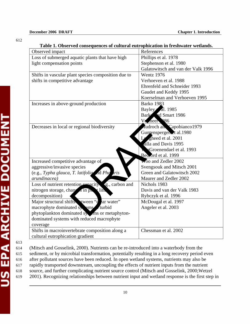
612 Table 1. Observed consequences of cultural eutrophication in freshwater wetlands.
Observed impact References Loss of submerged aquatic plants that have high light compensation points
Phillips et al. 1978 Stephenson et al. 1980 Galatowitsch and van der Valk 1996
Shifts in vascular plant species composition due to shifts in competitive advantage
Wentz 1976 Verhoeven et al. 1988 Ehrenfeld and Schneider 1993 Gaudet and Keddy 1995 Koerselman and Verhoeven 1995
Increases in above-ground production Barko 1983 Bayley et al. 1985 Barko and Smart 1986 Vermeer 1986
Decreases in local or regional biodiversity Mudroch and Capobianco1979 Guntenspergen et al.1980 Lougheed et al. 2001 Balla and Davis 1995 VanGroenendael et al. 1993 Bedford et al. 1999
Increased competitive advantage of aggressive/invasive species (e.g., Typha glauca, T. latifolia and Phalaris arundinacea)
Woo and Zedler 2002 Svengsouk and Mitsch 2001 Green and Galatowitsch 2002 Maurer and Zedler 2002
Loss of nutrient retention capacity (e.g., carbon and nitrogen storage, changes in plant litter decomposition)
Nichols 1983 Davis and van der Valk 1983 Rybczyk et al. 1996
Major structural shifts between “clear water” macrophyte dominated systems to turbid phytoplankton dominated systems or metaphyton-dominated systems with reduced macrophyte coverage
McDougal et al. 1997 Angeler et al. 2003
Shifts in macroinvertebrate composition along a cultural eutrophication gradient
Chessman et al. 2002
613 (Mitsch and Gosselink, 2000). Nutrients can be re-introduced into a waterbody from the 614 sediment, or by microbial transformation, potentially resulting in a long recovery period even 615 after pollutant sources have been reduced. In open wetland systems, nutrients may also be 616 rapidly transported downstream, uncoupling the effects of nutrient inputs from the nutrient 617 source, and further complicating nutrient source control (Mitsch and Gosselink, 2000;Wetzel 618 2001). Recognizing relationships between nutrient input and wetland response is the first step in 619
DRAFT

December 2006 DRAFT Chapter 1. Introduction
11
mitigating the effects of cultural eutrophication. Once relationships are established, nutrient 620 criteria can be developed to manage nutrient pollution and protect wetlands from eutrophication. 621 622 623 1.4 OVERVIEW OF THE CRITERIA DEVELOPMENT PROCESS 624
625 This section describes the five general elements of nutrient criteria development outlined in the 626 National Strategy (USEPA 1998a). A prescriptive, one-size-fits-all approach is not appropriate 627 due to regional differences that exist and the scientific community’s limited technical 628 understanding of the relationship between nutrients, algal and macrophyte growth, and other 629 factors (e.g., flow, light, substrata). The approach chosen for criteria development therefore may 630 be tailored to meet the specific needs of each State or Tribe. 631 632 The USEPA is utilizing the following principal elements from the National Strategy for the 633 Development of Regional Nutrient Criteria (1998a). This document can be downloaded in PDF 634 format at the following website: http://www.epa.gov/waterscience/criteria/nutrient/strategy.html. 635 636 1. EPA will develop Ecoregional recommended nutrient criteria to account for the natural 637
variation existing across various parts of the country. Different waterbody processes and 638 responses dictate that nutrient criteria be specific to the waterbody type. No single 639 criterion is sufficient for each (or all) waterbody types; therefore, we anticipate system 640 classification within each waterbody type for appropriate criteria derivation. 641 642
643 2. EPA guidance documents for nutrient criteria will provide methodologies for developing 644
nutrient criteria for primary variables by ecoregion and waterbody type. 645 646 3. Regional Nutrient Coordinators will lead State/Tribal technical and financial support 647
operations used to compile data and conduct environmental investigations. Regional 648 technical assistance groups (RTAGs) with broad participation from regional and national 649 experts on nutrients and nutrient cycling will provide technical assistance and support. A 650 team of agency specialists from USEPA Headquarters will provide additional technical 651 and financial support to the Regions, and will establish and maintain communications 652 between the Regions and Headquarters. 653
654 4. Numeric nutrient criteria, developed at the national level from existing databases and 655
additional environmental investigations, will be used by EPA to derive specific 656 recommended criterion values. 657
658 5. Nationally developed ecoregional recommended nutrient criteria may be used by States 659
and Tribes as a point of departure for the development of more refined locally and 660 regionally appropriate criteria. 661 662
DRAFT

December 2006 DRAFT Chapter 1. Introduction
12
6. Nutrient criteria will serve as benchmarks for evaluating the relative success of any 663 nutrient management effort, whether protection or remediation is involved. EPA’s 664 recommended criteria will be re-evaluated periodically to assess whether refinements or 665 other improvements are needed. 666
667 The U. S. EPA Strategy envisions a process by which State/Tribal waters are initially monitored, 668 reference conditions are established, individual waterbodies are compared to known reference 669 waterbodies, and appropriate management measures are implemented. These measurements can 670 be used to document change and monitor the progress of nutrient reduction activities. 671 672 The National Nutrient Program represents an effort and approach to criteria development that, in 673 conjunction with efforts made by State and Tribal water quality managers, will ultimately result 674 in a heightened understanding of nutrient-response relationships. As the proposed process is put 675 into use to set criteria, program success will be gauged over time through evaluation of 676 management and monitoring efforts. A more comprehensive knowledge-base pertaining to 677 nutrient, and vegetation and /or algal relationships will be expanded as new information is 678 gained and obstacles overcome, justifying potential refinements to the criteria development 679 process described here. 680 681 The overarching goal of developing nutrient criteria is to ensure the quality of our national 682 waters. Ensuring water quality may include restoration of impaired systems, conservation of high 683 quality waters, and protection of systems at high risk for future impairment. The specific goals of 684 a State or Tribal water quality program may be defined differently based on the needs of each 685 State or Tribe, but should, at a minimum, be established to protect the designated uses for the 686 waterbodies within State or Tribal lands. In addition, as numeric nutrient criteria are developed 687 for the nation’s waters, States, Tribes and Territories should revisit their goals for water quality 688 and adapt their water quality standards as needed. 689 690 691 1.5 ROADMAP TO THE DOCUMENT 692
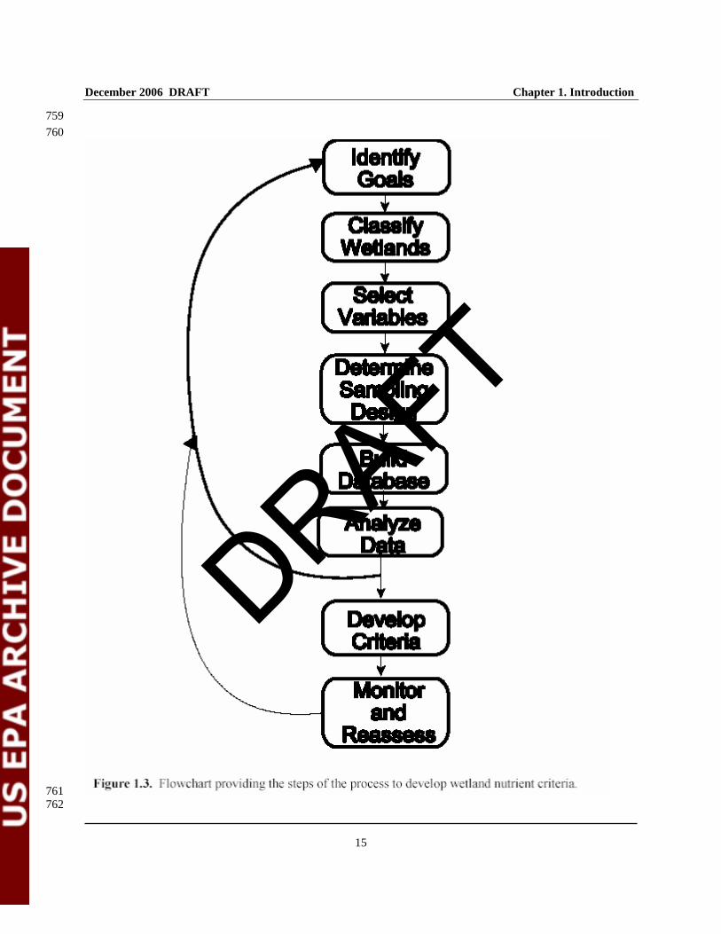
693 As set out in Figure 1.1, the process of developing numeric nutrient criteria begins with defining 694 the goals of criteria development and standards adoption. Those goals are pertinent to the 695 classification of systems, the development of a monitoring program, and the application of 696 numeric nutrient criteria to permit limits and water quality protection. These goals therefore 697 should be determined with the intent of revising and adapting them as new information is 698 obtained and the paths to achieving those goals are clarified. Defining the goals for criteria 699 development is the first step in the process. The summaries below describe each chapter in this 700 document. The document is written to provide a stepwise procedure for criteria development. 701 Some chapters contain information that is not needed by some readers; the descriptions below 702 should serve as a guide to the most relevant information for each reader. 703 704
DRAFT

December 2006 DRAFT Chapter 1. Introduction
13
Chapter Two describes many of the functions of wetland systems and their role in the landscape 705 with respect to nutrients. This chapter is intended to familiarize the reader with some basic 706 scientific information about wetlands that will provide a better understanding of how nutrients 707 move within a wetland and the importance of wetland systems in the landscape. 708 709 Chapter Three discusses wetland classification and presents the reader with options for 710 classifying wetlands based on system characteristics. This chapter introduces the scientific 711 rationale for classifying wetlands, reviews some common classification schemes, and discusses 712 their role in establishing nutrient criteria for wetlands. The classification of these systems is 713 important to identifying their nutrient status and their condition in relation to similar wetlands. 714 715 Chapter Four provides technical guidance on designing effective sampling programs for State 716 and Tribal wetland water quality monitoring programs. Most States and Tribes should begin 717 wetland monitoring programs to collect water quality and biological data in order to develop 718 nutrient criteria protective of wetland systems. The best monitoring programs are designed to 719 assess wetland condition with statistical rigor and maximize effective use of available resources. 720 The sampling protocol selected, therefore, should be determined based on the goals of the 721 monitoring program, and the resources available. 722 723 Chapter Five gives an overview of candidate variables that could be used to establish nutrient 724 criteria for wetlands. Primary variables are expected to be most broadly useful in characterizing 725 wetland conditions with respect to nutrients and include nutrient loading rates, soil nutrient 726 concentrations, and nutrient content of wetland vegetation. Supporting variables provide 727 information useful for normalizing causal and response variables. The candidate variables 728 suggested here are not the only parameters that can be used to determine wetland nutrient 729 condition, but rather identify those variables that are thought to be most likely to identify the 730 current nutrient condition and will be most useful in determining a change in nutrient status. 731 732 A database of relevant water quality information can be an invaluable tool to States and Tribes as 733 they develop nutrient criteria. If little or no data are available for most regions or parameters, it 734 may be necessary for States and Tribes to create a database of newly gathered data. Chapter Six 735 provides the basic information on how to develop a database of nutrient information for 736 wetlands, and supplies links to ongoing database development efforts at the state and national 737 levels. 738 739 The purpose of Chapter Seven is to explore methods for analyzing data that can be used to 740 develop nutrient criteria. Proper analysis and interpretation of data determine the scientific 741 defensibility and effectiveness of the criteria. This chapter describes recommended approaches to 742 data analysis for developing numeric nutrient criteria for wetlands. Included are techniques to 743 evaluate metrics, to examine or compare distributions of nutrient exposure or response variables, 744 and to examine nutrient exposure-response relationships. 745 746
DRAFT

December 2006 DRAFT Chapter 1. Introduction
14
Chapter Eight describes the details of setting scientifically defensible criteria in wetlands. 747 Several approaches are presented that water quality managers can use to derive numeric criteria 748 for wetland systems in their State/Tribal waters. They include: (1) the use of the reference 749 conditions concept to characterize natural or minimally impaired wetland systems with respect to 750 causal and response variables, (2) applying predictive relationships to select nutrient 751 concentrations that will protect wetland function, and (3) developing criteria from established 752 nutrient exposure-response relationships (as in the peer-reviewed published literature). This 753 chapter provides information on how to determine the appropriate numeric criterion based on the 754 data collected and analyzed. 755 756 The appendices include a glossary of terms and acronyms, and case study examples of wetland 757 nutrient enrichment and management. 758
DRAFT
December 2006 DRAFT Chapter 1. Introduction
15
759 760
761 762
DRAFT
December 2006- DRAFT Chapter 2. Overview of Wetland Science
16
Chapter 2 Overview of Wetland Science 763 764 765 2.1 INTRODUCTION 766
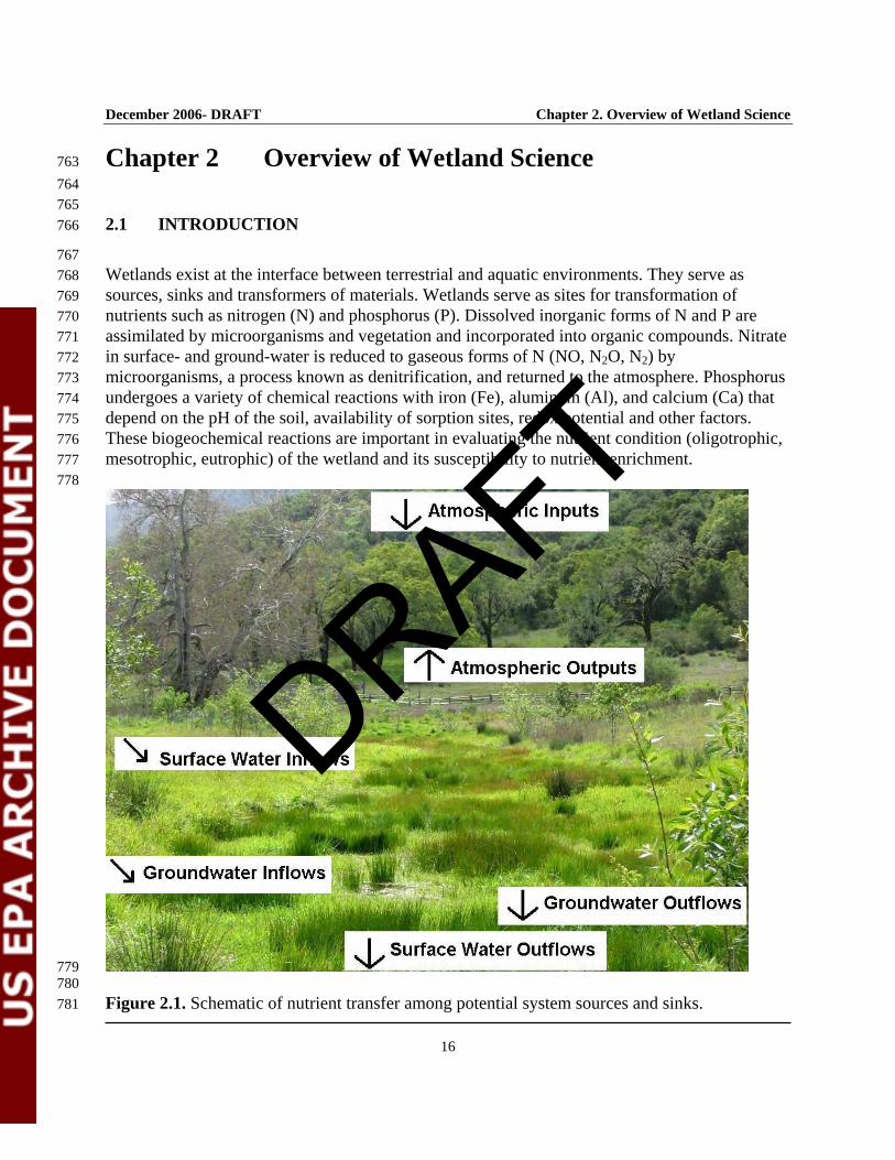
767 Wetlands exist at the interface between terrestrial and aquatic environments. They serve as 768 sources, sinks and transformers of materials. Wetlands serve as sites for transformation of 769 nutrients such as nitrogen (N) and phosphorus (P). Dissolved inorganic forms of N and P are 770 assimilated by microorganisms and vegetation and incorporated into organic compounds. Nitrate 771 in surface- and ground-water is reduced to gaseous forms of N (NO, N2O, N2) by 772 microorganisms, a process known as denitrification, and returned to the atmosphere. Phosphorus 773 undergoes a variety of chemical reactions with iron (Fe), aluminum (Al), and calcium (Ca) that 774 depend on the pH of the soil, availability of sorption sites, redox potential and other factors. 775 These biogeochemical reactions are important in evaluating the nutrient condition (oligotrophic, 776 mesotrophic, eutrophic) of the wetland and its susceptibility to nutrient enrichment. 777 778
779 780 Figure 2.1. Schematic of nutrient transfer among potential system sources and sinks. 781
DRAFT
December 2006- DRAFT Chapter 2. Overview of Wetland Science
17
782 Wetlands also generally are sinks for sediment, and wetlands that are connected to adjacent 783 aquatic ecosystems (e.g., rivers, estuaries) trap more sediment as compared to wetlands that lack 784 such connectivity. Wetlands also may be sources of organic carbon (C) and N to aquatic 785 ecosystems. Production of plant biomass (leaves, wood, roots) from riparian, alluvial and 786 floodplain forests and from fringe wetlands such as tidal marshes and mangroves provide organic 787 matter to support heterotrophic foodwebs of streams, rivers, estuaries and nearshore waters. 788 789 790 2.2 COMPONENTS OF WETLANDS 791
792 Wetlands are distinguished by three primary components: hydrology, soils and vegetation. 793 Wetland hydrology is the driving force that determines soil development, the assemblage of 794 plants and animals that inhabit the site, and the type and intensity of biochemical processes. 795 Wetland soils may be either organic or mineral, but share the characteristic that they are 796 saturated or flooded at least some of the time during the growing season. Wetland vegetation 797 consists of many species of algae, rooted plants that may be herbaceous and emergent, such as 798 cattail (Typha sp.) and arrowhead (Saggitaria sp.), or submergent, such as pondweeds 799 (Potamogeton sp.), or may be woody such as bald cypress (Taxodium distichum) and tupelo 800 (Nyssa aquatica). Depending on the duration, depth and frequency of inundation or saturation, 801 wetland plants may be either obligate (i.e., species found almost exclusively in wetlands) or 802 facultative (i.e., species found in wetlands but which also may be found in upland habitats). The 803 discussion that follows provides an overview of wetland hydrology, soils and vegetation, as well 804 as aspects of biogeochemical cycling in these systems. 805 806 HYDROLOGY 807 808 Hydrology is characterized by water source, hydroperiod (depth, duration and frequency of 809 inundation or soil saturation), and hydrodynamics (direction and velocity of water movement). 810 The hydrology of wetlands differs from that of terrestrial ecosystems in that wetlands are 811 inundated or saturated long enough during the growing season to produce soils that are at least 812 periodically deficient in oxygen. Wetlands differ from other aquatic ecosystems by their shallow 813 depth of inundation that enables rooted vegetation to become established, in contrast to deep 814 water aquatic ecosystems, where the depth and duration of inundation can be too great to support 815 emergent vegetation. Anaerobic soils promote colonization by vegetation adapted to low 816 concentrations of oxygen in the soil. 817 818 Wetlands can receive water from three sources: precipitation, surface flow and groundwater 819 (Figure 2.2). The relative proportion of these hydrologic inputs influences the plant communities 820 that develop, the type of soils that form, and the predominant biogeochemical processes. 821 Wetlands that receive mostly precipitation tend to be “closed” systems with little exchange of 822 materials with adjacent terrestrial or aquatic ecosystems. Examples of precipitation-driven 823
DRAFT

December 2006- DRAFT Chapter 2. Overview of Wetland Science
18
GRO
UND WATE
R PRECIPITATION
SURFACE FLOW
Riverine, Fringe, Tidal
Bogs, Pocosins
Fens, Seeps
0%
0%0%
33%
33%
33%
67%
67%
67%
100%
100%100%
Figure 2. Relationship between water source and wetland vegetation. Modified from Brinson (1993).
wetlands include “ombrotrophic” bogs and depressional wetlands such as cypress domes and 824 vernal pools. Wetlands that receive water mostly from surface flow tend to be “open” systems 825 with large exchanges of water 826 827 829 831 833 835 837 839 841 843 845 847 849 851 853 855 857 859 861 863 865 867 869 871 and 873
materials between the wetland and adjacent non-wetland ecosystems. Examples include 877 floodplain forests and fringe wetlands such as lakeshore marshes, tidal marshes and mangroves. 878 Wetlands that receive primarily groundwater inputs tend to have more stable hydroperiods than 879 precipitation- and surface water-driven wetlands and, depending on the underlying bedrock or 880 parent material, high concentrations of dissolved inorganic constituents such as calcium (Ca) and 881 magnesium (Mg). Fen wetlands and seeps are examples of groundwater-fed wetlands. 882 883 Hydroperiod is highly variable depending on the type of wetland. Some wetlands that receive 884 most of their water from precipitation (e.g.,vernal pools) have very short duration hydroperiods. 885 Wetlands that receive most of their water from surface flooding (e.g.,floodplain swamps) often 886 are flooded longer and to a greater depth than precipitation-driven wetlands. Fringe wetlands 887 such as tidal marshes and mangroves are frequently flooded (up to twice daily) by astronomical 888
DRAFT
December 2006- DRAFT Chapter 2. Overview of Wetland Science
19
tides but the duration of inundation is relatively short. In groundwater-fed wetlands, hydroperiod 889 is more stable and water levels are relatively constant as compared to precipitation- and surface 890 water-driven wetlands, because groundwater provides a near-constant input of water throughout 891 the year. 892 893 Hydrodynamics is especially important in the exchange of materials between wetlands and 894 adjacent terrestrial and aquatic ecosystems. In fact, the role of wetlands as sources, sinks and 895 transformers of material depends, in large part, on hydrodynamics. For example, many wetlands 896 are characterized by lateral flow of surface- or ground-water. Flow of water can be unidirectional 897 or bidirectional. An example of a wetland with unidirectional flow is a floodplain forest where 898 surface water spills over the river bank, travels through the floodplain and re-enters the river 899 channel some distance downstream. In fringe wetlands such as lakeshore marshes, tidal marshes 900 and mangroves, flow is bidirectional as wind-driven or astronomical tides transport water into, 901 then out of the wetland. These wetlands have the ability to intercept sediment and dissolved 902 inorganic and organic materials from adjacent systems as water passes through the wetland. In 903 precipitation-driven wetlands, flow may occur more in the vertical direction as rainfall percolates 904 through the (unsaturated) surface soil down to the water table. Wetlands with lateral surface flow 905 may be important in maintaining water quality of adjacent aquatic systems by trapping sediment 906 and other pollutants. Surface flow wetlands also may be an important source of organic C to 907 aquatic ecosystems as detritus, particulate C and dissolved organic C are transported out of the 908 wetland into rivers and streams down gradient or to adjacent lakes, estuaries and nearshore 909 waters. 910 911 SOILS 912 913 Wetland soils, also known as hydric soils, are defined as “soils that formed under conditions of 914 saturation, flooding or ponding long enough during the growing season to develop anaerobic 915 conditions in the upper part” (NRCS 1998). Anaerobic conditions result because the rate of 916 oxygen diffusion through water is approximately 10,000 times less than in air. Wetland soils 917 may be composed mostly of mineral constituents (sand, silt, clay) or they may contain large 918 amounts of organic matter. Because anaerobic conditions slow or inhibit decomposition of 919 organic matter, wetland soils typically contain more organic matter than terrestrial soils of the 920 same region or climatic conditions. Under conditions of near continuous inundation or 921 saturation, organic soils (histosols) may develop. Histosols are characterized by high organic 922 matter content, 20-30% (12-18% organic C depending on clay content) with a thickness of at 923 least 40 cm (USDA 1999). Because of their high organic matter content, Histosols possess 924 physical and chemical properties that are much different from mineral wetland soils. For 925 example, organic soils generally have lower bulk densities, higher porosity, greater water 926 holding capacity, lower nutrient availability, and greater cation exchange capacity than many 927 mineral soils. 928 929
DRAFT

December 2006- DRAFT Chapter 2. Overview of Wetland Science
20
Mineral wetland soils, in addition to containing greater amounts of sand, silt and clay than 930 histosols, are distinguished by changes in soil color that occur when elements such as Fe and 931 manganese (Mn) are reduced by microorganisms under anaerobic conditions. Reduction of Fe 932 leads to the development of grey or “gleyed” soil color as oxidized forms of Fe (ferric Fe, Fe3+) 933 are converted to reduced forms (ferrous Fe, Fe+2). In sandy soils, development of a dark-colored 934 organic-rich surface layer is used to distinguish hydric soil from non-hydric (terrestrial) soil. An 935 organic-rich surface layer, indicative of periodic inundation or saturation, is not sufficiently thick 936 (<40 cm) to qualify as a histosol which forms under near-continuous inundation. 937 938 Wetland soils serve as sites for many biogeochemical transformations. They also provide long 939 and short term storage of nutrients for wetland plants. Wetland soils are typically anaerobic 940 within a few millimeters of the soil-water interface. Water column oxygen concentrations are 941 often depressed due to the slow rate of oxygen diffusion through water. However, even when 942 water column oxygen concentrations are supported by advective currents, high rates of oxygen 943 consumption lead to the formation of a very thin oxidized layer at the soil-water interface. 944 Similar oxidized layers can also be found surrounding roots of wetland plants. Many wetland 945 plants are known to transport oxygen into the root zone, thus creating aerobic zones in 946 predominantly anaerobic soil. The presence of these aerobic (oxidizing) zones within the 947 reducing environment in saturated soils allows for the occurrence of oxidative and reductive 948 transformations to occur in close proximity to each other. For example, ammonia is oxidized to 949 nitrate within the aerobic zone surrounding plant roots in a process called nitrification. Nitrate 950 then readily diffuses into adjacent anaerobic soil, where it is reduced to molecular nitrogen via 951 denitrification or may be reduced to ammonium in certain conditions through dissimilatory 952 nitrate reduction (Mitsch and Gosselink 2000; Ruckauf et al., 2004; Reddy and Delaune, 2005). 953 The anaerobic environment hosts the transformations of N, P, sulfur (S), Fe, Mn, and C. Most of 954 these transformations are microbially mediated. The oxidized soil surface layer also is important 955 to the transport and translocation of transformed constituents, providing a barrier to translocation 956 of some reduced constituents. These transformations will be discussed in more detail below in 957 Biogeochemical Cycling. 958 959 VEGETATION 960 961 Wetland plants consist of macrophytes and microphytes. Macrophytes include free-floating, 962 submersed, floating-leaved and rooted emergent plants. Microphytes are algae that may be free 963 floating or attached to macrophyte stems and other surfaces. Plants require oxygen to meet 964 respiration demands for growth, metabolism and reproduction. In macrophytes, much (about 965 50%) of the respiration occurs below ground in the roots. Wetland macrophytes, however, live in 966 periodically to continuously-inundated and saturated soils and, so, use specialized adaptations to 967 grow in anaerobic soils. Adaptations consist of morphological/anatomical adaptations that result 968 in anoxia avoidance and metabolic adaptations that result in true tolerance to anoxia. 969 Morphological/anatomic adaptations include shallow roots systems, aerenchyma, buttressed 970 trunks, pneumatophores (e.g., cypress “knees”) and lenticles on the stem. These adaptations 971
DRAFT

December 2006- DRAFT Chapter 2. Overview of Wetland Science
21
facilitate oxygen transport from the shoots to the roots where most respiration occurs. Many 972 wetland plants also possess metabolic adaptations, such as anaerobic pathways of respiration, 973 that produce non-toxic metabolites such as malate to mitigate the adverse effects of oxygen 974 deprivation, instead of toxic compounds like ethanol (Mendelssohn and Burdick 1988). 975 976 Species best adapted to anaerobic conditions are typically found in areas inundated for long 977 periods, whereas species less tolerant of anaerobic conditions are found in areas where 978 hydroperiod is shorter. For example, in southern forested wetlands, areas such as abandoned 979 river channels (oxbows) are dominated by obligate species such as bald cypress (Taxodium 980 distichum) and tupelo gum (Nyssa aquatica) (Wharton et al. 1982). Areas inundated less 981 frequently are dominated by hardwoods such as black gum (Nyssa sylvatica), green ash 982 (Fraxinus pennsylvanicus) and red maple (Acer rubrum) and the highest, driest wetland areas are 983 dominated by facultative species such as sweet gum (Liquidambar styraciflua) and sycamore 984 (Platanus occidentalis) (Wharton et al. 1982). Herbaceous-dominated wetlands also exhibit 985 patterns of zonation controlled by hydroperiod (Mitsch and Gosselink 2000). 986 987 In estuarine wetlands such as salt- and brackish-water marshes and mangroves, salinity and 988 sulfides also adversely affect growth and reproduction of vegetation. Inundation with seawater 989 brings dissolved salts (NaCl) and sulfate. Salt creates an osmotic imbalance in vegetation, 990 leading to dessication of plant tissues. However, many plant species that live in estuarine 991 wetlands possess adaptations to deal with salinity (Whipple et al., 1981; Zheng et al. 2004). 992 These adaptations include salt exclusion at the root surface, salt secreting glands on leaves, 993 schlerophyllous (thick, waxy) leaves, low transpiration rates and other adaptations to reduce 994 uptake of water and associated salt. Sulfate carried in by the tides undergoes sulfate reduction in 995 anaerobic soils to produce hydrogen sulfide (H2S) that, at high concentrations, is toxic to 996 vegetation. At sub-lethal concentrations, H2S inhibits nutrient uptake and impairs plant growth. 997 998 SOURCES OF NUTRIENTS 999 1000 Point Sources 1001 Point source discharges of nutrients to wetlands may come from municipal or industrial 1002 discharges, including stormwater runoff from municipalities or industries, or in some cases from 1003 large animal feeding operations. Nutrients from point source discharges may be controlled 1004 through the National Pollutant Discharge Elimination System (NPDES) permits, most of which 1005 are administered by states authorized to issue such permits. In general, point source discharges 1006 that are not stormwater related are fairly constant with respect to loadings. 1007 1008 Nonpoint Sources 1009 Nonpoint sources of nutrients are commonly discontinuous and can be linked to seasonal 1010 agricultural activity or other irregularly occurring events such as silviculture, non-regulated 1011 construction, and storm events. Nonpoint nutrient pollution from agriculture is most commonly 1012 associated with row crop agriculture, and livestock production that tend to be highly associated 1013
DRAFT
December 2006- DRAFT Chapter 2. Overview of Wetland Science
22
with rain events and seasonal land use activities. Nonpoint nutrient pollution from urban and 1014 suburban areas is most often associated with climatological events (rain, snow, and snowmelt) 1015 when pollutants are most likely to be transported to aquatic resources. 1016 1017 Runoff from agricultural and urban is generally thought to be the largest source of nonpoint 1018 source pollution; however growing evidence suggests that atmospheric deposition may have a 1019 significant influence on nutrient enrichment, particularly from nitrogen (Jaworski et al. 1997). 1020 Gases released through fossil fuel combustion and agricultural practices are two major sources of 1021 atmospheric N that may be deposited in waterbodies (Carpenter et al. 1998). Nitrogen and 1022 nitrogen compounds formed in the atmosphere return to the earth as acid rain or snow, gas, or 1023 dry particles. Atmospheric deposition, like other forms of pollution, may be determined at 1024 different scales of resolution. More information on national atmospheric deposition can be found 1025 at: http://www.arl.noaa.gov/research/programs/airmon.html; http://nadp.sws.uiuc.edu/. These 1026 national maps may provide the user with information about regional areas where atmospheric 1027 deposition, particularly of nitrogen, may be of concern. However, these maps are generally low 1028 resolution when considered at the local and site-specific scale and may not reflect areas of high 1029 local atmospheric deposition, such as local areas in a downwind plume from an animal feedlot 1030 operation. 1031 1032 Other nonpoint sources of nutrient pollution may include certain silviculture and mining 1033 operations; these activities generally constitute a smaller fraction of the national problem, but 1034 may be locally significant nutrient sources. Control of nonpoint source pollutants focuses on land 1035 management activities and regulation of pollutants released to the atmosphere (Carpenter et al. 1036 1998). 1037 1038 1039 2.3 WETLAND NUTRIENT COMPONENTS 1040
1041 NUTRIENT BUDGETS 1042 1043 Wetland nutrient inputs mirror wetland hydrologic inputs (e.g., precipitation, surface water, and 1044 ground water), with additional loading associated with atmospheric dry deposition and 1045 nitrification (Figures 2.5 and 2.6). Total atmospheric deposition (wet and dry) may be the 1046 dominant input for precipitation-dominated wetlands, while surface- or ground-water inputs may 1047 dominate other wetland systems. 1048 1049 The total annual nutrient load (mg-nutrients/yr) into a wetland is the sum of the dissolved and 1050 particulate loads. The dissolved load (mg-nutrients/s) can be estimated by multiplying the 1051 instantaneous inflow (L/s) by the nutrient concentration (mg-nutrients/L). EPA recommends 1052 calculating the annual load by the summation of this function over the year – greater loads may 1053 found during periods of increased flow so EPA recommends monitoring during these intervals. 1054 Where continuous data are unavailable, average flows and concentrations may be used if a bias 1055
DRAFT

December 2006- DRAFT Chapter 2. Overview of Wetland Science
23
factor (Cohn et al., 1989) is included to account for unmeasured loads during high flows. 1056 Particulate loads (kg-sediments/yr) can be estimated using the product of suspended and bedload 1057 inputs (kg-sediments/yr) and the mass concentrations (mg-nutrients/kg-sediment). 1058 1059 Surface-water nutrient inputs are associated with flows from influent streams, as well as diffuse 1060 sources from overland flow through the littoral zone. Ground-water inputs can also be 1061 concentrated at points (e.g., springs), or diffuse (such as seeps). The influence of allochthonous 1062 sources is likely to be greatest in those zones closest to the source. 1063 1064 Because wetlands generally tend to be low-velocity, depositional environments, they often 1065 sequester sediments and their associated nutrients. These sediment inputs generally accumulate 1066 at or near the point of entry into the wetland, forming deltas or levees near tributaries, or along 1067 the shoreline for littoral inputs. Coarser fractions (e.g., gravels and sands) tend to settle first, 1068 with the finer fractions (silts, clays, and organic matter) tend to settle further from the inlet point. 1069 Particulate input from ground-water sources can usually be neglected, while particulate inputs 1070 from atmospheric sources may be important if local or regional sources are present. 1071 1072 Wetland nutrient outputs again mirror hydrologic outputs (e.g., surface- and ground-water), and 1073 loads are again estimated as the product of the flow and the concentration of nutrients in the 1074 flow. While evaporation losses from wetlands may be significant, there are no nutrient losses 1075 associated with this loss. Instead, loss of nutrients to the atmosphere may occur as a result of 1076 ammonia volatilization, N2O losses from nitrification, as well as losses from incomplete 1077 denitrification. Because sediment outputs from wetlands may be minor, nutrient exports by this 1078 mechanism may not be important. 1079 1080 Nutrient accumulation in wetlands occurs when nutrient inputs exceed outputs. Net nutrient 1081 loads can be estimated as the difference between these inputs and outputs. It is important, 1082 therefore, to have some estimate of net accumulation by taking the difference between upstream 1083 and downstream loads. Sampling ground-water nutrient concentrations in wells located upstream 1084 and downstream of the wetland can provide some sense of net nutrient sequestration, while 1085 sampling wetland nutrient inflows and outflows is needed for determining the additional 1086 sequestration for this pathway. 1087 1088 BIOGEOCHEMICAL CYCLING 1089 1090 Biogeochemical cycling of nutrients in wetlands is governed by physical, chemical and 1091 biological processes in the soil and water column. Biogeochemical cycling of nutrients is not 1092 unique to wetlands, but the aerobic and anaerobic interface generally found in saturated soils of 1093 wetlands creates unique conditions that allow both aerobic and anaerobic processes to operate 1094 simultaneously. The hydrology and geomorphology of wetlands (Johnston et al. 2001) influences 1095 biogeochemical processes and constituent transport and transformation within the systems (e.g., 1096 water-sediment exchange, plant uptake, and export of organic matter). Interrelationships among 1097
DRAFT
December 2006- DRAFT Chapter 2. Overview of Wetland Science
24
hydrology, biogeochemistry, and the response of wetland biota vary among wetland types 1098 (Mitsch and Gosselink, 2000; Reddy and Delaune, 2005). 1099 1100 Biogeochemical processes in the soil and water column are key drivers of several ecosystem 1101 functions associated with wetland values (e.g., water quality improvement through 1102 denitrification, long-term nutrient storage in the organic matter) (Figure 2.3). The hub for 1103 biogeochemistry is organic matter and its cycling in the soil and water column. Nutrients such as 1104 N, P, and S are primary components of soil organic matter, and cycling of these nutrients is 1105 always coupled to C cycling. Many processes occur within the carbon, nitrogen, phosphorus and 1106 sulfur (C, N, P, or S) cycles; microbial communities mediate the rate and extent of these 1107 reactions in soil and the water column. 1108 1109 Aerobic-anaerobic interfaces are more common in wetlands than in upland landscapes and may 1110 occur at the soil-water interface, in the root zones of aquatic macrophytes, and at surfaces of 1111 detrital tissue and benthic periphyton mats. The juxtaposition of aerobic and anaerobic zones in 1112 wetlands supports a wide range of microbial populations and associated metabolic activities, 1113 with oxygen reduction occurring in the aerobic interface of the substrate, and reduction of 1114 alternate electron acceptors occurring in the anaerobic zone (D’Angelo and Reddy, 1994a or b). 1115 Under continuously saturated soil conditions, vertical layering of different metabolic activities 1116 can be present, with oxygen reduction occurring at and just below the soil-floodwater interface. 1117 Substantial aerobic decomposition of plant detritus occurs in the water column; however, the 1118 supply of oxygen may be insufficient to meet demands and drive certain microbial groups to 1119 utilize alternate electron acceptors (e.g., nitrate, oxidized forms of iron (Fe) and manganese 1120 (Mn), sulfate and bicarbonate (HCO3)). 1121 1122
DRAFT
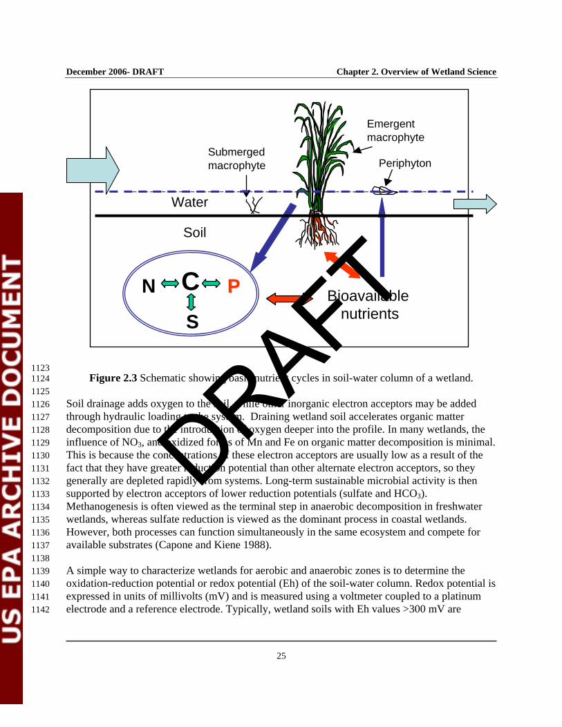
December 2006- DRAFT Chapter 2. Overview of Wetland Science
25
1123 Figure 2.3 Schematic showing basic nutrient cycles in soil-water column of a wetland. 1124
1125 Soil drainage adds oxygen to the soil, while other inorganic electron acceptors may be added 1126 through hydraulic loading to the system. Draining wetland soil accelerates organic matter 1127 decomposition due to the introduction of oxygen deeper into the profile. In many wetlands, the 1128 influence of NO3, and oxidized forms of Mn and Fe on organic matter decomposition is minimal. 1129 This is because the concentrations of these electron acceptors are usually low as a result of the 1130 fact that they have greater reduction potential than other alternate electron acceptors, so they 1131 generally are depleted rapidly from systems. Long-term sustainable microbial activity is then 1132 supported by electron acceptors of lower reduction potentials (sulfate and HCO3). 1133 Methanogenesis is often viewed as the terminal step in anaerobic decomposition in freshwater 1134 wetlands, whereas sulfate reduction is viewed as the dominant process in coastal wetlands. 1135 However, both processes can function simultaneously in the same ecosystem and compete for 1136 available substrates (Capone and Kiene 1988). 1137 1138 A simple way to characterize wetlands for aerobic and anaerobic zones is to determine the 1139 oxidation-reduction potential or redox potential (Eh) of the soil-water column. Redox potential is 1140 expressed in units of millivolts (mV) and is measured using a voltmeter coupled to a platinum 1141 electrode and a reference electrode. Typically, wetland soils with Eh values >300 mV are 1142
Water Soil
CN
S
PP Bioavailable nutrients
Periphyton
Emergent macrophyte
Submerged macrophyte
DRAFT
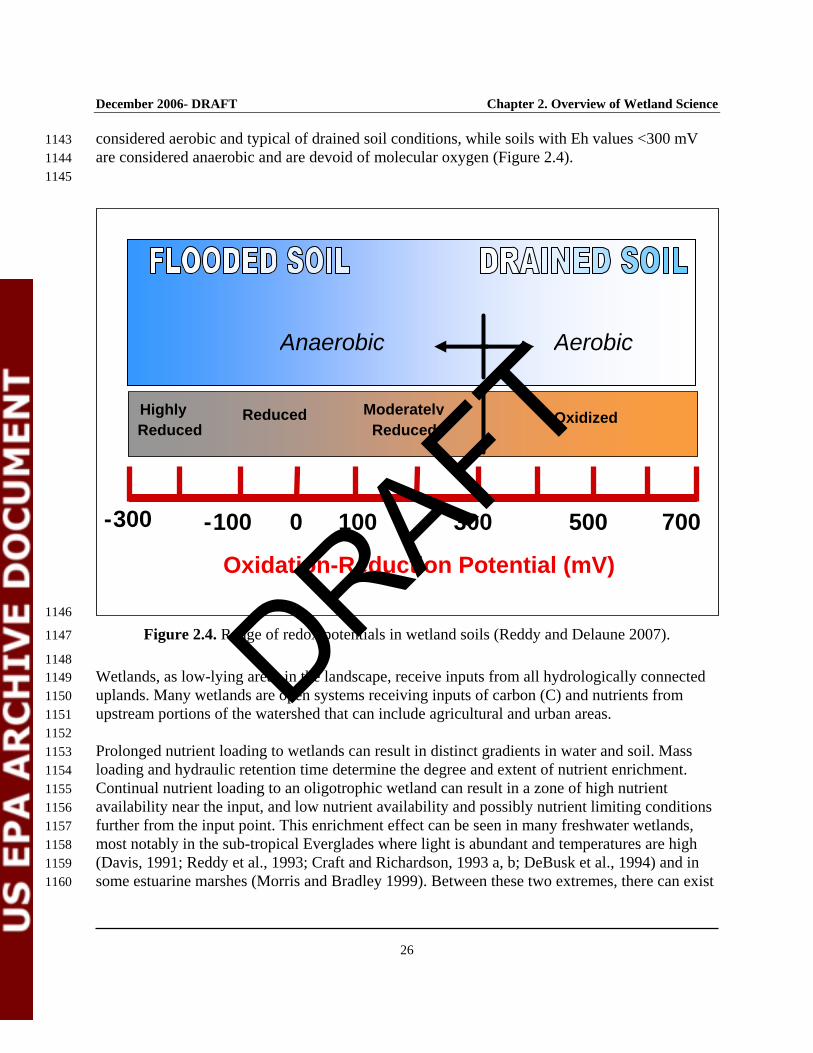
December 2006- DRAFT Chapter 2. Overview of Wetland Science
26
considered aerobic and typical of drained soil conditions, while soils with Eh values <300 mV 1143 are considered anaerobic and are devoid of molecular oxygen (Figure 2.4). 1144 1145
1146
Figure 2.4. Range of redox potentials in wetland soils (Reddy and Delaune 2007). 1147
1148 Wetlands, as low-lying areas in the landscape, receive inputs from all hydrologically connected 1149 uplands. Many wetlands are open systems receiving inputs of carbon (C) and nutrients from 1150 upstream portions of the watershed that can include agricultural and urban areas. 1151 1152 Prolonged nutrient loading to wetlands can result in distinct gradients in water and soil. Mass 1153 loading and hydraulic retention time determine the degree and extent of nutrient enrichment. 1154 Continual nutrient loading to an oligotrophic wetland can result in a zone of high nutrient 1155 availability near the input, and low nutrient availability and possibly nutrient limiting conditions 1156 further from the input point. This enrichment effect can be seen in many freshwater wetlands, 1157 most notably in the sub-tropical Everglades where light is abundant and temperatures are high 1158 (Davis, 1991; Reddy et al., 1993; Craft and Richardson, 1993 a, b; DeBusk et al., 1994) and in 1159 some estuarine marshes (Morris and Bradley 1999). Between these two extremes, there can exist 1160
- 300 700 0 300 500 100 -100
Highly Reduced
Reduced ModeratelyReduced
Oxidized
Anaerobic Aerobic
Oxidation-Reduction Potential (mV)
DRAFT
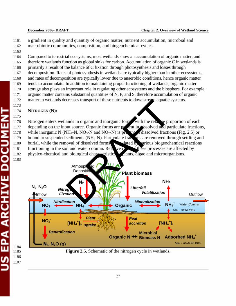
December 2006- DRAFT Chapter 2. Overview of Wetland Science
27
a gradient in quality and quantity of organic matter, nutrient accumulation, microbial and 1161 macrobiotic communities, composition, and biogeochemical cycles. 1162 1163 Compared to terrestrial ecosystems, most wetlands show an accumulation of organic matter, and 1164 therefore wetlands function as global sinks for carbon. Accumulation of organic C in wetlands is 1165 primarily a result of the balance of C fixation through photosynthesis and losses through 1166 decomposition. Rates of photosynthesis in wetlands are typically higher than in other ecosystems, 1167 and rates of decomposition are typically lower due to anaerobic conditions, hence organic matter 1168 tends to accumulate. In addition to maintaining proper functioning of wetlands, organic matter 1169 storage also plays an important role in regulating other ecosystems and the biosphere. For example, 1170 organic matter contains substantial quantities of N, P, and S, therefore accumulation of organic 1171 matter in wetlands decreases transport of these nutrients to downstream aquatic systems. 1172 1173 NITROGEN (N): 1174 1175 Nitrogen enters wetlands in organic and inorganic forms, with the relative proportion of each 1176 depending on the input source. Organic forms are present in dissolved and particulate fractions, 1177 while inorganic N (NH4-N, NO3-N and NO2-N) is present in dissolved fractions (Fig. 2.5) or 1178 bound to suspended sediments (NH4-N). Particulate fractions are removed through settling and 1179 burial, while the removal of dissolved forms is regulated by various biogeochemical reactions 1180 functioning in the soil and water column. Relative rates of these processes are affected by 1181 physico-chemical and biological characteristics of plants, algae and microorganisms. 1182 1183
1184 Figure 2.5. Schematic of the nitrogen cycle in wetlands. 1185
1186 1187
Organic
Plant
uptake
Adsorbed NH4+
NO3-
Litterfall
Denitrification
Peataccretion
Organic N
Nitrification Mineralization
Plant biomass
[NH4+]s
NH4+
[NH4+]s
NH4NO3
NN2, N2O (g)
N2 N2O
Microbial Biomass N
NH3
Volatilization
N2 Nitrogen Fixation
Atmospheric Deposition
OutflowInflow
Water Column
Soil - ANAEROBIC
Soil - AEROBIC DRAFT
December 2006- DRAFT Chapter 2. Overview of Wetland Science
28
Nitrogen reactions in wetlands effectively process inorganic N through nitrification and 1188 denitrification, ammonia volatilization and plant uptake. These processes aid in lowering levels 1189 of inorganic N in the water column. A significant portion of dissolved organic N assimilated by 1190 plants is returned to the water column during breakdown of detrital tissue or soil organic matter, 1191 and the majority of this dissolved organic N is resistant to decomposition. Under these 1192 conditions, water leaving wetlands may contain elevated levels of N in organic form. Exchange 1193 of dissolved nitrogen species between soil and water column support several nitrogen reactions. 1194 For example, nitrification in the aerobic soil layer is supported by ammonium flux from the 1195 anaerobic soil layer. Similarly, denitrification in the anaerobic soil layer is supported by nitrate 1196 flux from the aerobic soil layer and water column. Relative rates of these reactions will, 1197 however, depend on the environmental conditions present in the soil and water column (Reddy 1198 and Delaune 2007). 1199 1200 PHOSPHORUS (P): 1201 1202 Phosphorus retention by wetlands is regulated by physical (sedimentation and entrainment), 1203 chemical (precipitation and flocculation), and biological mechanisms (uptake and release by 1204 vegetation, periphyton and microorganisms). Phosphorus in the influent water is found in 1205 soluble and particulate fractions, with both fractions containing a certain proportion of inorganic 1206 and organic forms. Relative proportions of these pools depend on the input source. For example, 1207 municipal wastewater may contain a large proportion (>75%) as inorganic P in soluble forms, as 1208 compared to effluents from agricultural watersheds where a greater percentage of P loading may 1209 be in the particulate fraction. 1210 1211 Phosphorus forms that enter a wetland are grouped into: (i) dissolved inorganic P (DIP), (ii) 1212 dissolved organic P (DOP), (iii) particulate inorganic P (PIP), and (iv) particulate organic P 1213 (POP) (Figure 2.6). The particulate and soluble organic fractions may be further separated into 1214 labile and refractory components. Dissolved inorganic P is generally bioavailable, whereas 1215 organic and particulate P forms generally must be transformed into inorganic forms before 1216 becoming bioavailable. Both biotic and abiotic mechanisms regulate relative pool sizes and 1217 transformations of P compounds within the water column and soil. Alterations in these fractions 1218 can occur during flow through wetlands and depend on the physical, chemical, and biological 1219 characteristics of the systems. Thus, both biotic and abiotic processes should be considered when 1220 evaluating P retention capacities of wetlands. Biotic processes include; assimilation by 1221 vegetation, plankton, periphyton and microorganisms. Abiotic processes include sedimentation, 1222 adsorption by soils, precipitation, and exchange processes between soil and the overlying water 1223 column (Reddy et al. 1999; 2005; Reddy and Delaune, 2007). The processes affecting 1224 phosphorus exchange at the soil/sediment water interface include: (i) diffusion and advection due 1225 to wind-driven currents, (ii) diffusion and advection due to flow and bioturbation, (iii) processes 1226 within the water column (mineralization, sorption by particulate matter, and biotic uptake and 1227 release), (iv) diagenetic processes (mineralization, sorption and precipitation dissolution) in 1228
DRAFT
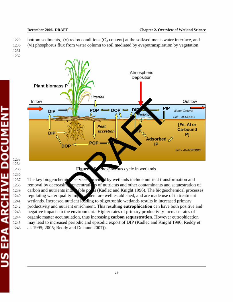
December 2006- DRAFT Chapter 2. Overview of Wetland Science
29
bottom sediments, (v) redox conditions (O2 content) at the soil/sediment -water interface, and 1229 (vi) phosphorus flux from water column to soil mediated by evapotranspiration by vegetation. 1230 1231 1232
1233 1234
Figure 2.6. Phosphorous cycle in wetlands. 1235 1236 The key biogeochemical services provided by wetlands include nutrient transformation and 1237 removal by decreasing concentrations of nutrients and other contaminants and sequestration of 1238 carbon and nutrients into stable pools (Kadlec and Knight 1996). The biogeochemical processes 1239 regulating water quality improvement are well established, and are made use of in treatment 1240 wetlands. Increased nutrient loading to oligotrophic wetlands results in increased primary 1241 productivity and nutrient enrichment. This resulting eutrophication can have both positive and 1242 negative impacts to the environment. Higher rates of primary productivity increase rates of 1243 organic matter accumulation, thus increasing carbon sequestration. However eutrophication 1244 may lead to increased periodic and episodic export of DIP (Kadlec and Knight 1996; Reddy et 1245 al. 1995; 2005; Reddy and Delaune 2007)). 1246
Water Column
Soil - ANAEROBIC
Peataccretion
[Fe, Al or Ca-bound
P] Adsorbed
IP
Litterfall
DOP
Plant biomass P
DIP PIP POP
DIP
POP DOPDOP
DIP
DIP
Outflow
Periphyton
Atmospheric Deposition
Inflow
Soil - AEROBIC
DRAFT
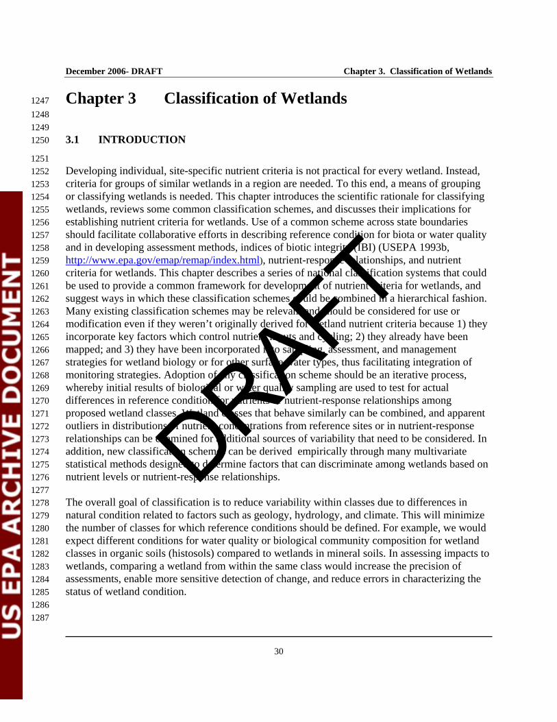
December 2006- DRAFT Chapter 3. Classification of Wetlands
30
Chapter 3 Classification of Wetlands 1247 1248 1249 3.1 INTRODUCTION 1250
1251 Developing individual, site-specific nutrient criteria is not practical for every wetland. Instead, 1252 criteria for groups of similar wetlands in a region are needed. To this end, a means of grouping 1253 or classifying wetlands is needed. This chapter introduces the scientific rationale for classifying 1254 wetlands, reviews some common classification schemes, and discusses their implications for 1255 establishing nutrient criteria for wetlands. Use of a common scheme across state boundaries 1256 should facilitate collaborative efforts in describing reference condition for biota or water quality 1257 and in developing assessment methods, indices of biotic integrity (IBI) (USEPA 1993b, 1258 http://www.epa.gov/emap/remap/index.html), nutrient-response relationships, and nutrient 1259 criteria for wetlands. This chapter describes a series of national classification systems that could 1260 be used to provide a common framework for development of nutrient criteria for wetlands, and 1261 suggest ways in which these classification schemes could be combined in a hierarchical fashion. 1262 Many existing classification schemes may be relevant and should be considered for use or 1263 modification even if they weren’t originally derived for wetland nutrient criteria because 1) they 1264 incorporate key factors which control nutrient inputs and cycling; 2) they already have been 1265 mapped; and 3) they have been incorporated into sampling, assessment, and management 1266 strategies for wetland biology or for other surface water types, thus facilitating integration of 1267 monitoring strategies. Adoption of any classification scheme should be an iterative process, 1268 whereby initial results of biological or water quality sampling are used to test for actual 1269 differences in reference condition for nutrients or nutrient-response relationships among 1270 proposed wetland classes. Wetland classes that behave similarly can be combined, and apparent 1271 outliers in distributions of nutrient concentrations from reference sites or in nutrient-response 1272 relationships can be examined for additional sources of variability that need to be considered. In 1273 addition, new classification schemes can be derived empirically through many multivariate 1274 statistical methods designed to determine factors that can discriminate among wetlands based on 1275 nutrient levels or nutrient-response relationships. 1276 1277 The overall goal of classification is to reduce variability within classes due to differences in 1278 natural condition related to factors such as geology, hydrology, and climate. This will minimize 1279 the number of classes for which reference conditions should be defined. For example, we would 1280 expect different conditions for water quality or biological community composition for wetland 1281 classes in organic soils (histosols) compared to wetlands in mineral soils. In assessing impacts to 1282 wetlands, comparing a wetland from within the same class would increase the precision of 1283 assessments, enable more sensitive detection of change, and reduce errors in characterizing the 1284 status of wetland condition. 1285 1286 1287
DRAFT
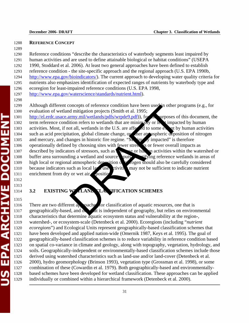
December 2006- DRAFT Chapter 3. Classification of Wetlands
31
REFERENCE CONCEPT 1288 1289 Reference conditions “describe the characteristics of waterbody segments least impaired by 1290 human activities and are used to define attainable biological or habitat conditions” (USEPA 1291 1990, Stoddard et al. 2006). At least two general approaches have been defined to establish 1292 reference condition - the site-specific approach and the regional approach (U.S. EPA 1990b, 1293 http://www.epa.gov/bioindicators/). The current approach to developing water quality criteria for 1294 nutrients also emphasizes identification of expected ranges of nutrients by waterbody type and 1295 ecoregion for least-impaired reference conditions (U.S. EPA 1998, 1296 http://www.epa.gov/waterscience/standards/nutrient.html). 1297 1298 Although different concepts of reference condition have been used in other programs (e.g., for 1299 evaluation of wetland mitigation projects (Smith et al. 1995; 1300 http://el.erdc.usace.army.mil/wetlands/pdfs/wrpde9.pdf)), for the purposes of this document, the 1301 term reference condition refers to wetlands that are minimally or least impacted by human 1302 activities. Most, if not all, wetlands in the U.S. are affected to some extent by human activities 1303 such as acid precipitation, global climate change, or other atmospheric deposition of nitrogen 1304 and mercury, and changes in historic fire regime. “Minimally impacted” is therefore 1305 operationally defined by choosing sites with fewer stressors or fewer overall impacts as 1306 described by indicators of stressors, such as land-use or human activities within the watershed or 1307 buffer area surrounding a wetland and source inputs. Identifying reference wetlands in areas of 1308 high local or regional atmospheric deposition of nitrogen should also be carefully considered 1309 because indicators such as local land use activities may not be sufficient to indicate nutrient 1310 enrichment from dry or wet air deposition. 1311 1312 1313 3.2 EXISTING WETLAND CLASSIFICATION SCHEMES 1314
1315 There are two different approaches for classification of aquatic resources, one that is 1316 geographically-based, and one that is independent of geography, but relies on environmental 1317 characteristics that determine aquatic ecosystem status and vulnerability at the region-, 1318 watershed-, or ecosystem-scale (Detenbeck et al. 2000). Ecoregions (including “nutrient 1319 ecoregions”) and Ecological Units represent geographically-based classification schemes that 1320 have been developed and applied nation-wide (Omernik 1987, Keys et al. 1995). The goal of 1321 geographically-based classification schemes is to reduce variability in reference condition based 1322 on spatial co-variance in climate and geology, along with topography, vegetation, hydrology, and 1323 soils. Geographically-independent or environmentally-based classification schemes include those 1324 derived using watershed characteristics such as land-use and/or land-cover (Detenbeck et al. 1325 2000), hydro geomorphology (Brinson 1993), vegetation type (Grossman et al. 1998), or some 1326 combination of these (Cowardin et al. 1979). Both geographically-based and environmentally-1327 based schemes have been developed for wetland classification. These approaches can be applied 1328 individually or combined within a hierarchical framework (Detenbeck et al. 2000). 1329
DRAFT
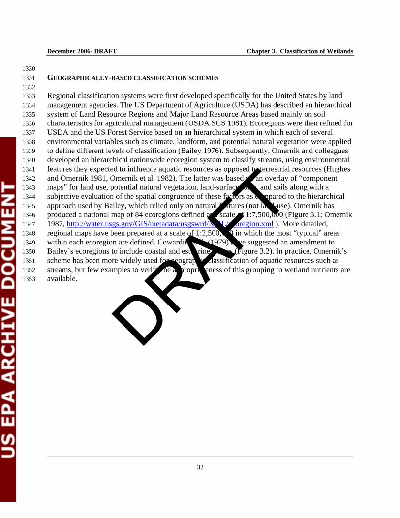
December 2006- DRAFT Chapter 3. Classification of Wetlands
32
1330 GEOGRAPHICALLY-BASED CLASSIFICATION SCHEMES 1331 1332 Regional classification systems were first developed specifically for the United States by land 1333 management agencies. The US Department of Agriculture (USDA) has described an hierarchical 1334 system of Land Resource Regions and Major Land Resource Areas based mainly on soil 1335 characteristics for agricultural management (USDA SCS 1981). Ecoregions were then refined for 1336 USDA and the US Forest Service based on an hierarchical system in which each of several 1337 environmental variables such as climate, landform, and potential natural vegetation were applied 1338 to define different levels of classification (Bailey 1976). Subsequently, Omernik and colleagues 1339 developed an hierarchical nationwide ecoregion system to classify streams, using environmental 1340 features they expected to influence aquatic resources as opposed to terrestrial resources (Hughes 1341 and Omernik 1981, Omernik et al. 1982). The latter was based on an overlay of “component 1342 maps” for land use, potential natural vegetation, land-surface form, and soils along with a 1343 subjective evaluation of the spatial congruence of these factors as compared to the hierarchical 1344 approach used by Bailey, which relied only on natural features (not land-use). Omernik has 1345 produced a national map of 84 ecoregions defined at a scale of 1:7,500,000 (Figure 3.1; Omernik 1346 1987, http://water.usgs.gov/GIS/metadata/usgswrd/XML/ecoregion.xml ). More detailed, 1347 regional maps have been prepared at a scale of 1:2,500,000 in which the most “typical” areas 1348 within each ecoregion are defined. Cowardin et al. (1979) have suggested an amendment to 1349 Bailey’s ecoregions to include coastal and estuarine waters (Figure 3.2). In practice, Omernik’s 1350 scheme has been more widely used for geographic classification of aquatic resources such as 1351 streams, but few examples to verify the appropriateness of this grouping to wetland nutrients are 1352 available. 1353
DRAFT
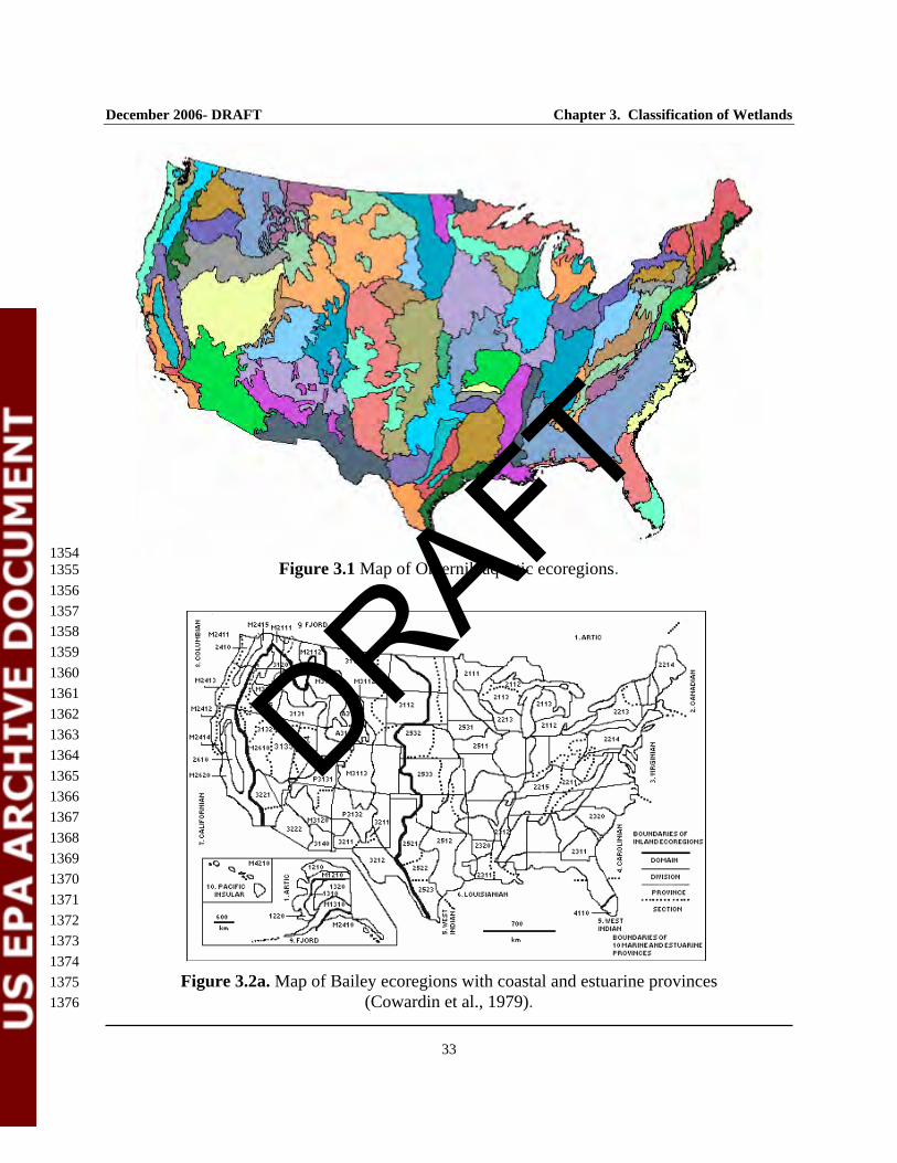
December 2006- DRAFT Chapter 3. Classification of Wetlands
33
1354 Figure 3.1 Map of Omernik aquatic ecoregions. 1355
1356 1357 1358 1359 1360 1361 1362 1363 1364 1365 1366 1367 1368 1369 1370 1371 1372 1373 1374
Figure 3.2a. Map of Bailey ecoregions with coastal and estuarine provinces 1375 (Cowardin et al., 1979). 1376
DRAFT

December 2006- DRAFT Chapter 3. Classification of Wetlands
34
Figure 3.2b. Legend 1377
1378
DRAFT
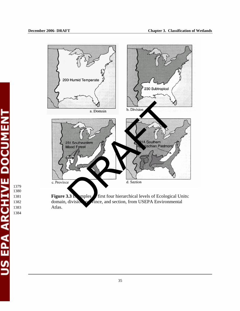
December 2006- DRAFT Chapter 3. Classification of Wetlands
35
1379 1380
Figure 3.3 Examples of first four hierarchical levels of Ecological Units: 1381 domain, division, province, and section, from USEPA Environmental 1382 Atlas. 1383
1384 DRAFT
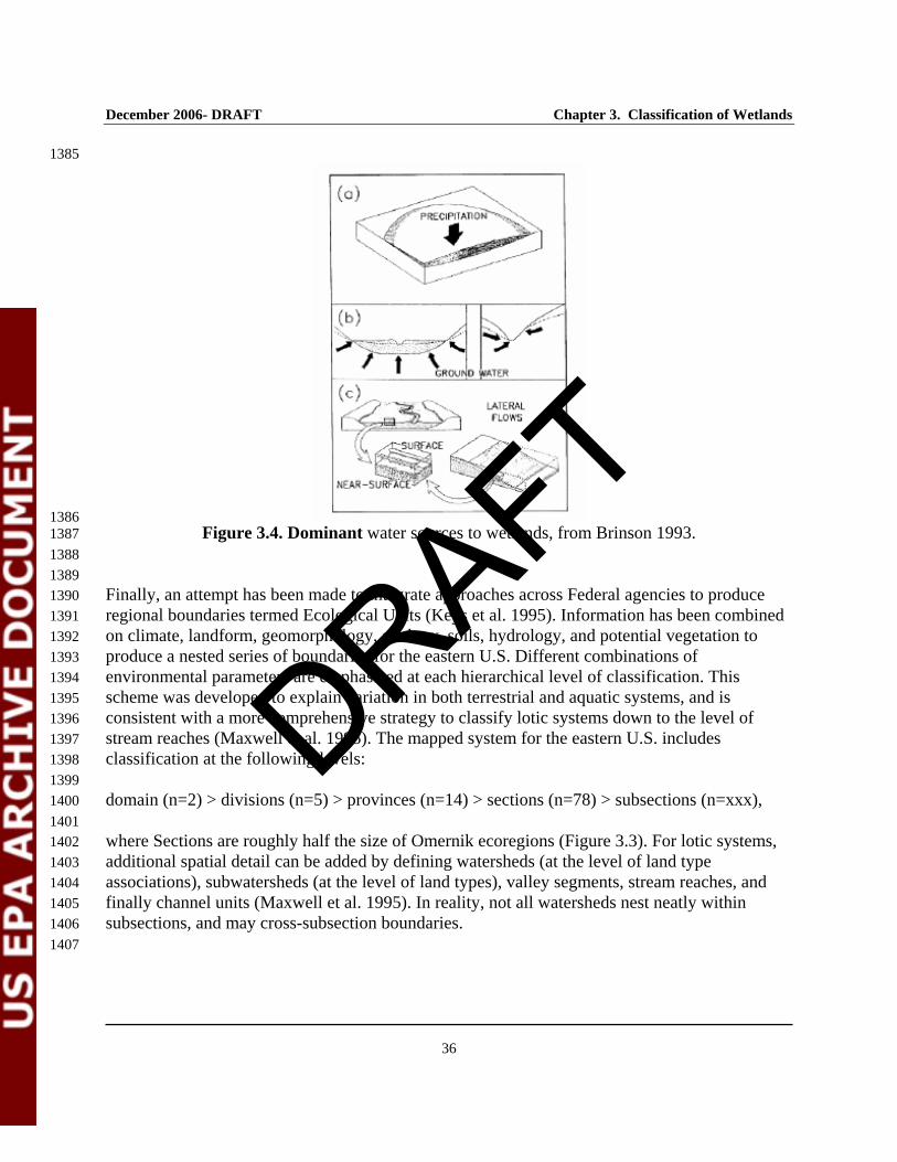
December 2006- DRAFT Chapter 3. Classification of Wetlands
36
1385
1386 Figure 3.4. Dominant water sources to wetlands, from Brinson 1993. 1387
1388 1389 Finally, an attempt has been made to integrate approaches across Federal agencies to produce 1390 regional boundaries termed Ecological Units (Keys et al. 1995). Information has been combined 1391 on climate, landform, geomorphology, geology, soils, hydrology, and potential vegetation to 1392 produce a nested series of boundaries for the eastern U.S. Different combinations of 1393 environmental parameters are emphasized at each hierarchical level of classification. This 1394 scheme was developed to explain variation in both terrestrial and aquatic systems, and is 1395 consistent with a more comprehensive strategy to classify lotic systems down to the level of 1396 stream reaches (Maxwell et al. 1995). The mapped system for the eastern U.S. includes 1397 classification at the following levels: 1398 1399 domain (n=2) > divisions (n=5) > provinces (n=14) > sections (n=78) > subsections (n=xxx), 1400 1401 where Sections are roughly half the size of Omernik ecoregions (Figure 3.3). For lotic systems, 1402 additional spatial detail can be added by defining watersheds (at the level of land type 1403 associations), subwatersheds (at the level of land types), valley segments, stream reaches, and 1404 finally channel units (Maxwell et al. 1995). In reality, not all watersheds nest neatly within 1405 subsections, and may cross-subsection boundaries. 1406 1407
DRAFT
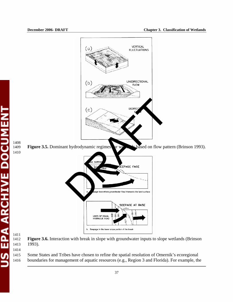
December 2006- DRAFT Chapter 3. Classification of Wetlands
37
1408 Figure 3.5. Dominant hydrodynamic regimes for wetlands based on flow pattern (Brinson 1993). 1409 1410
1411 Figure 3.6. Interaction with break in slope with groundwater inputs to slope wetlands (Brinson 1412 1993). 1413
1414 Some States and Tribes have chosen to refine the spatial resolution of Omernik’s ecoregional 1415 boundaries for management of aquatic resources (e.g., Region 3 and Florida). For example, the 1416
DRAFT
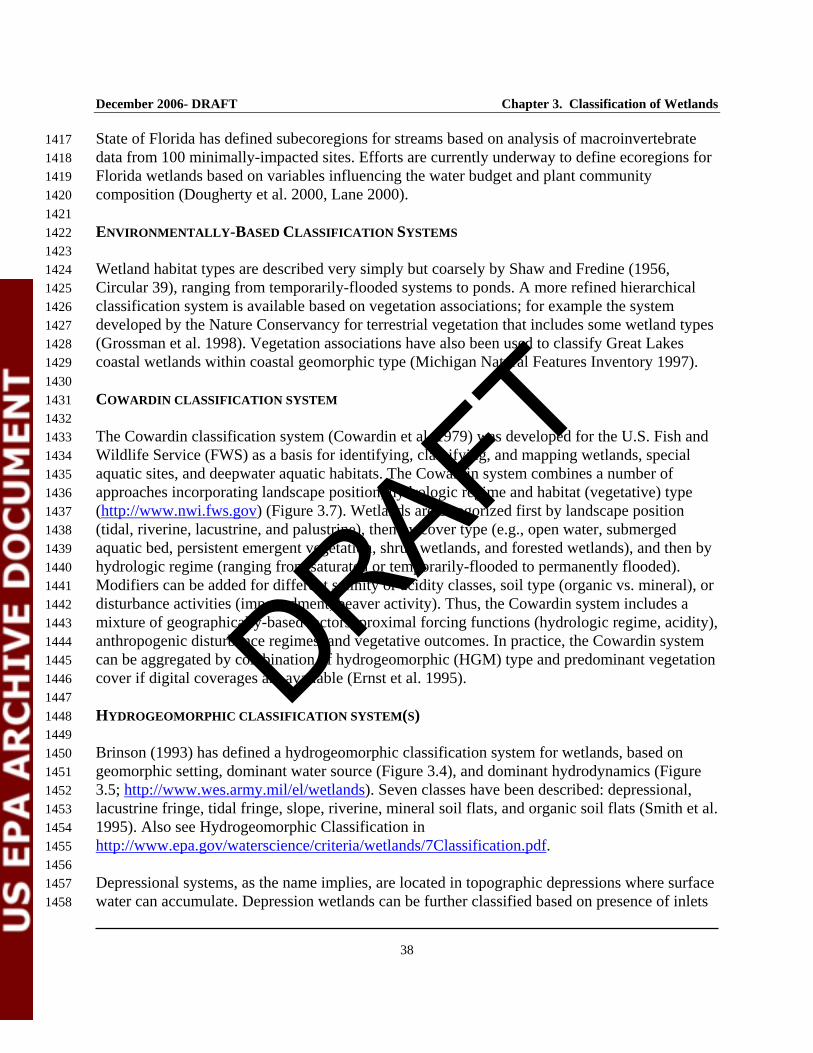
December 2006- DRAFT Chapter 3. Classification of Wetlands
38
State of Florida has defined subecoregions for streams based on analysis of macroinvertebrate 1417 data from 100 minimally-impacted sites. Efforts are currently underway to define ecoregions for 1418 Florida wetlands based on variables influencing the water budget and plant community 1419 composition (Dougherty et al. 2000, Lane 2000). 1420 1421 ENVIRONMENTALLY-BASED CLASSIFICATION SYSTEMS 1422 1423 Wetland habitat types are described very simply but coarsely by Shaw and Fredine (1956, 1424 Circular 39), ranging from temporarily-flooded systems to ponds. A more refined hierarchical 1425 classification system is available based on vegetation associations; for example the system 1426 developed by the Nature Conservancy for terrestrial vegetation that includes some wetland types 1427 (Grossman et al. 1998). Vegetation associations have also been used to classify Great Lakes 1428 coastal wetlands within coastal geomorphic type (Michigan Natural Features Inventory 1997). 1429 1430 COWARDIN CLASSIFICATION SYSTEM 1431 1432 The Cowardin classification system (Cowardin et al. 1979) was developed for the U.S. Fish and 1433 Wildlife Service (FWS) as a basis for identifying, classifying, and mapping wetlands, special 1434 aquatic sites, and deepwater aquatic habitats. The Cowardin system combines a number of 1435 approaches incorporating landscape position, hydrologic regime and habitat (vegetative) type 1436 (http://www.nwi.fws.gov) (Figure 3.7). Wetlands are categorized first by landscape position 1437 (tidal, riverine, lacustrine, and palustrine), then by cover type (e.g., open water, submerged 1438 aquatic bed, persistent emergent vegetation, shrub wetlands, and forested wetlands), and then by 1439 hydrologic regime (ranging from saturated or temporarily-flooded to permanently flooded). 1440 Modifiers can be added for different salinity or acidity classes, soil type (organic vs. mineral), or 1441 disturbance activities (impoundment, beaver activity). Thus, the Cowardin system includes a 1442 mixture of geographically-based factors, proximal forcing functions (hydrologic regime, acidity), 1443 anthropogenic disturbance regimes, and vegetative outcomes. In practice, the Cowardin system 1444 can be aggregated by combination of hydrogeomorphic (HGM) type and predominant vegetation 1445 cover if digital coverages are available (Ernst et al. 1995). 1446 1447 HYDROGEOMORPHIC CLASSIFICATION SYSTEM(S) 1448 1449 Brinson (1993) has defined a hydrogeomorphic classification system for wetlands, based on 1450 geomorphic setting, dominant water source (Figure 3.4), and dominant hydrodynamics (Figure 1451 3.5; http://www.wes.army.mil/el/wetlands). Seven classes have been described: depressional, 1452 lacustrine fringe, tidal fringe, slope, riverine, mineral soil flats, and organic soil flats (Smith et al. 1453 1995). Also see Hydrogeomorphic Classification in 1454 http://www.epa.gov/waterscience/criteria/wetlands/7Classification.pdf. 1455 1456 Depressional systems, as the name implies, are located in topographic depressions where surface 1457 water can accumulate. Depression wetlands can be further classified based on presence of inlets 1458
DRAFT
December 2006- DRAFT Chapter 3. Classification of Wetlands
39
or outlets and primary water source as closed, open/groundwater, or open/surface water 1459 subclasses. 1460 1461 Lacustrine fringe wetlands are located along lake shores where the water elevation of the lake 1462 determines the water table of the adjacent wetland. Great Lakes coastal wetlands represent one 1463 important region of lacustrine fringe wetlands. These coastal systems are strongly influenced by 1464 coastal forming processes, and, as such, have been further classified by geomorphic type through 1465 various schemes (Jaworski and Raphael 1979, and others summarized in Michigan Natural 1466 Features Inventory 1997). These geomorphic coastal positions will further influence the 1467 predominant source of water and the degree and type of energy regime (riverine vs. seiche and 1468 wave activity). Tidal fringe wetlands occupy a similar position relative to marine coasts and 1469 estuaries, where water level is influenced by sea level. Tidal fringe wetlands can be broken down 1470 further based on salinity into euhaline vs. mixohaline subclasses. Slope wetlands occur on slopes 1471 where groundwater discharges to the land surface but typically do not have the capacity for 1472 surface water storage (Figure 3.6). Riverine wetlands are found in floodplains and riparian zones 1473 associated with stream channels. Riverine systems can be broken down based on watershed 1474 position (and thus hydrologic regime) into tidal, lower perennial, upper perennial, and 1475 nonperennial subclasses. Mineral soil flats are in areas of low topographic relief (e.g., 1476 interfluves, relic lake bottoms, and large floodplain terraces) with precipitation as the main 1477 source of water. The topography of organic soil flats (e.g., peatlands), in contrast, is controlled 1478 by the vertical accretion of organic matter. 1479 1480 The HGM classification system is being further refined to the subclass level for different regions 1481 or states and classes (Cole et al. 1997, http://www.wes.army.mil/el/wetlands). In addition to the 1482 classification factors described above, Clairain (2002) suggests using parameters such as the 1483 degree of connection between the wetland and other surface waters (depressional wetlands), 1484 salinity gradients (tidal), degree of slope or channel gradient (slope and riverine wetlands), 1485 position in the landscape (riverine, slope), and a scaling factor (stream order, watershed size or 1486 floodplain width for riverine subclasses). In some cases, existing regional schemes have been 1487 used as the basis for subclass definition (e.g., Stewart and Kantrud 1971, Golet and Larson 1974, 1488 Wharton et al. 1982, Weakley and Schafale 1991, Keough et al. 1999). 1489 1490 The HGM classification system has been applied primarily to assess wetland functions related to 1491 hydrology, biological productivity, biogeochemical cycling, and habitat (Smith et al. 1995, 1492 http://www.wes.army.mil/el/wetlands/pdfs/wrpde9.pdf ). The same environmental parameters 1493 that influence wetland functions also determine hydrologic characteristics and background water 1494 quality, which in turn drive wetland habitat structure and community composition, and the 1495 timing of biotic events. Thus, the HGM classification system can serve as a basis for partitioning 1496 variability in reference trophic status and biological condition, as well as defining temporal 1497 strategies for sampling. 1498 1499 1500
DRAFT
December 2006- DRAFT Chapter 3. Classification of Wetlands
40
COMPARISON OF ENVIRONMENTALLY-BASED CLASSIFICATION SYSTEMS 1501 1502 If an integrated assessment of aquatic resources within a watershed or region is desired, it may 1503 be useful to consider intercomparability of classification schemes for wetlands, lakes, and 1504 riverine systems to promote cost-effective sampling and ease of interpretation. The HGM 1505 approach could integrate readily with a finer level of classification for lake type because lentic 1506 systems are separated out as lacustrine fringe or depressional wetlands based on lake or pond 1507 size and influence of water level on the adjacent wetland. Lacustrine classification systems for 1508 water quality have included geography (climate + bedrock characteristics, Gorham et al. 1983) 1509 or hydrologic setting (Winter 1977, Eilers et al. 1983) as factors for categorization. McKee et al. 1510 (1992) suggest a modification of Cowardin’s system, for Great Lakes coastal wetlands 1511 incorporating landscape position (system), depth zone (littoral vs. limnetic subsystems), 1512 vegetative or substrate cover (class and subclass), and modifiers of ecoregions, water level 1513 regimes, fish community structure, geomorphic structure, and human modification. In contrast, 1514 the Michigan Natural Features Inventory (1997) categorizes Great Lakes coastal wetlands by 1515 Great Lake, then nine unique geomorphic types within lakes, then vegetative association. 1516 1517 For lotic systems, Brinson et al. (1995) describes an approach to further classify riverine classes 1518 into subclasses based on watershed position and stream size/permanence. This strategy is 1519 consistent with current monitoring efforts to develop stream IBIs (Indices of Biotic Integrity), 1520 which typically use stream order as a surrogate for watershed size in explaining additional 1521 background variation in IBI scores (USEPA 1996). A more detailed classification of stream 1522 reach types, based on hydrogeomorphic character, is described by Rosgen (1996). This 1523 classification scheme has been predominantly applied to assessments of channel stability and 1524 restoration options, and not to development of criteria. Gephardt et al. (1990) described a cross-1525 walk between riparian and wetland classification and description procedures. 1526 1527 DRAFT

December 2006- DRAFT Chapter 3. Classification of Wetlands
41
1528 Figure 3.7. (Top) Cowardin hierarchy of habitat types for estuarine systems; 1529
(Bottom) Palustrine systems, from Cowardin et al. 1979. 1530 1531
DRAFT
December 2006- DRAFT Chapter 3. Classification of Wetlands
42
COMBINATIONS OF GEOGRAPHIC AND ENVIRONMENTALLY-BASED APPROACHES 1532 1533 It is possible to combine geographically-based classification with hydrogeomorphic and/or 1534 habitat-based approaches. For example, a scheme could be defined that nests Cowardin 1535 (Cowardin et al. 1979) vegetative cover class within HGM class within ecoregion. Maxwell et al. 1536 (1995) have defined a scheme for linking geographically-based units based on geoclimatic 1537 setting (domains => divisions => provinces => sections => subsections) to watersheds and 1538 subwatersheds , and thus to riverine systems composed of valley segments, stream reaches, and 1539 channel units, or to lacustrine systems composed of lakes, lake depth zones, and lake 1540 sites/habitat types. 1541 1542 Maxwell et al. (1995) also define a series of fundamental hydrogeomorphic criteria for 1543 classifying wetlands based on Brinson (1993) and Winter (1992), including physiography 1544 (landscape position), water source, hydrodynamics, and climate. The first three of these are 1545 similar to the HGM classification system, whereas moisture regimes and soil temperature 1546 regimes are generally consistent at the province level (see summary tables in Keys et al. 1995). 1547 Finer scale variation in landforms is captured at the level of sections and below, which in turn 1548 will determine the dominance of different hydrogeomorphic classes of wetlands and associated 1549 surface waters (lakes and rivers). Characteristics and relative advantages and disadvantages of 1550 different classification systems are summarized in Table 2. 1551 1552 1553 3.3 SOURCES OF INFORMATION FOR MAPPING WETLAND CLASSES 1554
1555 In order to select wetlands for sampling in a random- or random-stratified design (described in 1556 Chapter 4), it is important to have a record of wetland locations to choose from, preferably 1557 categorized by the classification system of interest. For some, but not all portions of the country, 1558 wetlands have been mapped from aerial photography through the National Wetlands Inventory 1559 (NWI) maintained by the U.S. Fish and Wildlife Service (http://www.fws.gov/nwi/; Dahl 2005). 1560 In other cases, individual states have developed inventories, or researchers have developed lists 1561 for specific types of wetlands within a given region, e.g., Great Lakes coastal wetlands 1562 (Herdendorf et al. 1981). In order to sample these mapped wetland areas in a random fashion, it 1563 is important to have a list of each wetland that occurs within each class and its associated area. A 1564 geographic information system (GIS) allows one to automatically produce a list of all wetland 1565 polygons by type within a specified geographic region. Sources of digital information for 1566 mapping and/or classifying wetlands in a GIS are presented in the Land-Use Characterization for 1567 Nutrient and Sediment Risk Assessment Module 1568 (http://www.epa.gov/waterscience/criteria/wetlands/17LandUse.pdf). In areas for which digital 1569 NWI maps do not yet exist, potential wetland areas can be mapped using GIS tools 1570
DRAFT

December 2006- DRAFT Chapter 3. Classification of Wetlands
43
1571
Table 2. Comparison of landscape and wetland classification schemes.
Classification scheme
Scale Hierarchical? Levels of strata Advantages Disadvantages Potential links with other schemes
Bailey’s ecoregions Nationwide Yes Domains Divisions Provinces Sections
Only natural attributes included
Digital maps
Terrestrial basis Untested for wetlands No hydrology
Could form first strata for any of the schemes below ecological units
Omernik ecoregions Nationwide No Ecoregions Subecoregions
Digital maps Combines land-use with natural attributes
Untested for most wetlands
No hydrology
Could form first strata for any of the schemes below ecological units
Ecological units (Maxwell et al. 1995)
Nationwide Yes Domain Divisions Provinces Sections Subsections
Digital maps Greater number of strata and units than for ecoregions
Untested for wetlands
Could form first strata for any of the schemes below ecological units
Ties to classification schemes already defined within hydrogeomorphic types
US ACE Hydrogeomorphic Classes
Nationwide at class level; regionalized at subclass level
Yes - limited Class Subclass
Specific for wetlands
Subclasses not comparable across different regions
Intermediate strata between geographic and habitat-scale
Rosgen channel types
Nationwide Yes Level I Level II
Captures differences in hydrologic regime for riverine wetlands
More focused on instream channel form than riparian characteristics
Riverine only Not mapped
Intermediate strata between hydro-geomorphic type and habitat-scale
DRAFT

December 2006- DRAFT Chapter 3. Classification of Wetlands
44
Table 2. Comparison of landscape and wetland classification schemes.
Classification scheme
Scale Hierarchical? Levels of strata Advantages Disadvantages Potential links with other schemes
Anderson land-cover classes
Nationwide Yes Level I Level II Level III
Common basis for land-use/land-cover mapping
Not functionally based Cross-walk w NWI system possible
Circular 39 classes Nationwide No Class Popular recognition
Mixture of criteria used to distinguish classes
Not mapped
Strata below geographic but contains mixture of hydrogeomorphic type and habitat type
National Wetland Inventory
Nationwide Yes System Subsystem Class Subclass Hydrologic modifier Other modifiers
Digital maps available for much of nation (but smallest wetlands omitted)
Inconsistencies in mapping water quality modifiers
Limited consideration of hydrogeomorphic type
Strata below geographic Hydrogeomorphic class could be
improved by link w HGM system
Vegetation associations
International Yes System Formation class Formation subclass Formation group Formation subgroup Formation alliance Association
Consistency across terrestrial and aquatic systems
Not functionally based No digital maps Taxa specific
Could be used as lowest level within other schemes
1572 DRAFT

December 2006- DRAFT Chapter 3. Classification of Wetlands
45
to predict relative wetness (e.g., Phillips 1990) or soil survey maps with hydric soil series can be 1573 used. It should be noted that in areas in which hydrology has been significantly altered 1574 (e.g.,through ditching, tiling, or construction of urban stormwater systems), areas of potential 1575 wetlands could have been removed already. Similarly, although there are no current maps of 1576 wetlands by hydrogeomorphic class, these could be derived through GIS techniques using a 1577 combination of wetland coverages, hydrography (adjacency to large lakes and rivers), and digital 1578 elevation models to derive landforms (mineral and organic soil flats) and/or landscape position 1579 (slope and depressional wetlands). 1580 1581 1582 3.4 DIFFERENCES IN NUTRIENT REFERENCE CONDITION OR SENSITIVITY 1583
TO NUTRIENTS AMONG WETLAND CLASSES 1584
1585 Very few studies to verify classification systems for wetland nutrient monitoring have been 1586 completed, although a number of monitoring strategies have been implemented based on pre-1587 selected strata. Monitoring efforts to develop or assess biological criteria generally have used a 1588 combination of geographic region and hydrogeomorphic class or subclass (e.g.,Cole et al. 1997, 1589 Bennett 1999, Apfelbeck 1999, Michigan Natural Features Inventory 1997). Analysis of plant 1590 associations has been used to derive empirical classifications based on factors such as landscape 1591 position, water source, climate, bedrock, and sediment hydraulic conductivity (Weakley and 1592 Schafale 1991, Nicholson 1995, Halsey et al. 1997, Michigan Natural Features Inventory 1997). 1593 Only one case of classification based on wetland macroinvertebrate composition was found. For 1594 Australian wetlands, wetland classes grouped by macroinvertebrate communities were 1595 distinguished by water chemistry extremes (low pH, high salinity), degree of nutrient 1596 enrichment, and water color (Growns et al. 1992). 1597 1598 In some cases (e.g., northern peatlands) classification criteria derived on the basis of plant 1599 associations are less powerful in discriminating among nutrient regimes (e.g.,Nicholson 1995); 1600 this may be particularly true where variation in vegetation type is related to differences in major 1601 ion chemistry and pH rather than nutrients. The same is true in southern pocosins, where short 1602 and tall pocosins differ in seasonal hydrology but not soil chemistry. However, when contrasting 1603 pocosins and swamp forests, soil nutrients differed strongly (Bridgham and Richardson 1993). 1604 For some potential indicators of nutrient status such as vegetation N:P ratios, indicator 1605 thresholds will be consistent across species (Koerselman and Meuleman 1996), while response 1606 thresholds for other indicators of plant nutrient status vary across functional plant groupings with 1607 different life history strategies. These differences may indicate potential differences in sensitivity 1608 to excess nutrient loading (McJannet et al. 1995). Thus, vegetation community types are not 1609 always a good predictor of background nutrient concentrations (reference condition) or 1610 sensitivity to nutrient loading. 1611 1612 Sensitivity to nutrient loading (as evidenced by differences in nutrient cycling and availability) 1613 may also be related to differences in hydroperiod among wetlands. Wetland mesocosms exposed 1614
DRAFT
December 2006- DRAFT Chapter 3. Classification of Wetlands
46
to pulse discharges had higher nutrient loss from the water column than those exposed to 1615 continuous flow regimes (Busnardo et al. 1992). Depending on the predominant mechanism for 1616 nutrient loss (e.g., plant uptake versus denitrification), nutrient-controlled primary production 1617 could be either stimulated or reduced. Mineralization rates of carbon, nitrogen, and phosphorus 1618 differ significantly among soils from northern Minnesota wetlands, related to an ombrotrophic to 1619 minerotrophic gradient (i.e., degree of groundwater influence) and aeration status (Bridgham et 1620 al. 1998). 1621 1622 In general, very few definitive tests of alternative classification schemes for wetlands are 1623 available with respect to describing reference condition for either nutrient criteria or biocriteria. 1624 However, evidence from the literature suggests that in many cases, both geographic factors (e.g., 1625 climate, geologic setting) and landscape setting (hydrogeomorphic type) are expected to affect 1626 both water quality and biotic communities. 1627 1628 1629 3.5 RECOMMENDATIONS 1630
1631 Classification strategies for nutrient criteria development should incorporate factors affecting 1632 background nutrient levels and wetland sensitivity to nutrient loading at several spatial scales. 1633 1634
• Classification of physiographic regions eliminates background variation in lithology and 1635 soil texture (affecting background nutrient levels and sorption capacity), in climate 1636 (affecting seasonality, productivity, decomposition and peat formation), and in 1637 landforms, which determines the predominance of different hydrogeomorphic classes. 1638
1639 • Classification by hydrogeomorphic class reduces background variation in predominant 1640
water and nutrient sources, water depth and dynamics, hydraulic retention time, 1641 assimilative capacity, and interactions with other surface water types (Table 3). 1642
1643 • Classification by water depth and duration (which may or may not be incorporated into 1644
hydrogeomorphic classes) helps to explain variation in internal nutrient cycling, 1645 dissolved oxygen level and variation, and the ability of wetlands to support some higher 1646 trophic levels such as fish and amphibians. 1647
1648 • Classification by vegetation type or zone, whether to inform site selection or to determine 1649
sampling strata within a site helps to explain background variation in predominant 1650 primary producer form (which will affect endpoint selection), as well as turnover rate and 1651 growth rates (which will affect rapidity of response to nutrient loadings). 1652
1653 In general, the choice of specific alternatives among the classification schemes listed above 1654 depends both on their intrinsic value as well as practical considerations, e.g., whether a 1655 classification scheme is available in mapped digital form or can be readily derived from 1656
DRAFT

December 2006- DRAFT Chapter 3. Classification of Wetlands
47
existing map layers, whether a hydrogeomorphic or other classification scheme has been 1657 refined for a particular region and wetland type, and whether classification schemes are 1658 already in use for monitoring and assessment of other waterbody types in a state or region. 1659
DRAFT

December 2006- DRAFT Chapter 3. Classification of Wetlands
48
Table 3. Features of the major hydrogeomorphic classes of wetlands that may influence background nutrient concentrations, sensitivity to nutrient loading, nutrient storage forms and assimilative capacity, designated use and choice of endpoints.
HGM Class Organic Flats Mineral Flats Depressional Riverine Fringe Slope
Predominant Nutrient Source(S)
Atmospheric Deposition
Atmospheric Deposition, Groundwater
Runoff (Particulate And Dissolved), Surface And Groundwater
Runoff (Particulate), Overbank Flooding (Particulate, Dissolved)
Adjacent Lake, Possible Stream Or Riverine Source, Groundwater
Groundwater
Landscape Position
Adjacent To Rivers Adjacent To Lakes Slope, Toe Of Slope
Hydrologic Regime Saturated, Little Standing Water
Saturated, Little Standing Water
Depth And Duration Vary From Saturated To Temporary To Seasonal To Semi-Permanent To Permanent Inundation
Depth, Duration Vary W River Flooding Regime
Standing Water In Emergent And Submerged Aquatic Zones, Short-Term Fluctuation Related To Seiche Activity, Long-Term To Wet-Dry Cycles
Saturated
Hydraulic Retention Time
Decades Decades Varies With Inflows/Outflows, Landscape Position
<Day To Few Days
< Day < Day
Nutrient Assimilation Capacity
Low High Sorption Capacity
High Sorption, Plant Uptake, (Limited) Sediment Storage
High Sorption, Sediment Trapping, Plant Uptake In Floodplain
Some Sediment Trapping Nutrient Transformer
High Sorption Capacity
DRAFT

December 2006- DRAFT Chapter 3. Classification of Wetlands
49
Table 3. Features of the major hydrogeomorphic classes of wetlands that may influence background nutrient concentrations, sensitivity to nutrient loading, nutrient storage forms and assimilative capacity, designated use and choice of endpoints.
HGM Class Organic Flats Mineral Flats Depressional Riverine Fringe Slope
Predominant Vegetation Growth Form
Mosses Sedges
Sedges Varies With Zone And Duration Of Flooding: Wooded Grass/Sedge Emergents Submerged Aquatics*
Wooded, Emergent Vegetation Submerged Aquatics*
Varies With Zone: Grass/Sedge Emergents Submerged Aquatics*
Wooded Grasses Sedges
Top Trophic Level Mammals Birds Amphibians Invertebrates
Mammals Birds Amphibians Invertebrates
Mammals Birds Mudminnows Amphibians Invertebrates
Fish Birds Mammals
Fish Birds Mammals
Mammals Birds Amphibians Invertebrates
Commercially-Important Fish/Wildlife
Waterfowl Fish* Waterfowl Fish*
Recreational Use Likely
Yes Yes Yes
Drinking Water Source Downstream
Possible Likely Possible
1660
Table 3 cont’d
DRAFT

December 2006- DRAFT Chapter 4. Sampling Design of Wetland Monitoring
50
Chapter 4 Sampling Design for Wetland Monitoring 1661
1662 4.1 INTRODUCTION 1663
1664 This chapter provides technical guidance on designing effective sampling programs for State and 1665 Tribal wetland water quality monitoring programs. EPA recommends that States and Tribes 1666 begin wetland monitoring programs to collect water quality and biological data in order to 1667 characterize the condition of existing wetlands as they develop nutrient criteria that protect their 1668 wetlands. The best monitoring programs are designed to assess wetland conditions with 1669 statistical rigor while maximizing available resources. 1670 1671 At the broadest level, monitoring data should: 1672 1673 1. Detect and characterize the condition of existing wetlands. 1674 1675 2. Describe whether wetland conditions are improving, degrading, or staying the same. 1676 1677 3. Define seasonal patterns, impairments, deviations in status in wetland conditions. 1678 1679 Water quality monitoring programs should collect a sufficient number of samples over time and 1680 space to identify changes in system condition or estimate average conditions with statistical 1681 rigor. Three approaches to study design for assessing water quality, biological and ecological 1682 condition, as well as identifying degradation in wetlands, are described in this chapter. Specific 1683 issues to consider in designing monitoring programs for wetland systems are also discussed in 1684 this chapter. The study designs presented here can be tailored to fit the goals of specific 1685 monitoring programs. 1686 1687 The three approaches described below (Section 4.3) (probabilistic sampling, targeted/tiered, and 1688 Before/After - Control/Impact [BACI]), present study designs that allow one to obtain a 1689 significant amount of information with relatively minimal effort. Probabilistic sampling begins 1690 with a large-scale random monitoring design that is reduced as the wetland system conditions are 1691 characterized. This approach is used to find the average condition of each wetland class in a 1692 specific region. Probabilistic sampling design is frequently used for new large scale monitoring 1693 programs at the State and Federal level (e.g., Environmental Monitoring and Assessment 1694 Program (EMAP), Regional Environmental Monitoring and Assessment Program (REMAP), 1695 State programs [e.g., Maine, Montana, Wisconsin]). The tiered or targeted approach to 1696 monitoring begins with coarse screening and proceeds to more detailed monitoring protocols as 1697 impaired and high-risk systems are identified and targeted for further investigation. Targeted 1698 sampling design provides a triage approach to more thoroughly assess condition and diagnose 1699 stressors in wetland systems in need of restoration, protection and intensive management. 1700 Several State pilot projects use this method or a modification of this method for wetland 1701
DRAFT

December 2006- DRAFT Chapter 4. Sampling Design of Wetland Monitoring
51
assessment (e.g., Florida, Ohio, Oregon, Minnesota). The synoptic approach described in 1702 Kentula et al. (1993) uses a modified targeted sampling design. The BACI design and its 1703 modifications are frequently used to assess the success of restoration efforts or other 1704 management experiments such as those describe in Case Study 2 in Appendix B2. BACI design 1705 allows for comparisons in similar systems over time to determine the rate of change in relation to 1706 the management activity, e.g., to assess the success of a wetland hydrologic restoration. 1707 Detenbeck et al. (1996) used BACI design for monitoring water quality of wetlands in the 1708 Minneapolis/St. Paul, Minnesota metro area. 1709 1710 Monitoring programs should be designed to describe what the current conditions are and to 1711 answer under what conditions impairment may occur. A well-designed monitoring program can 1712 contribute to determining those conditions. 1713 1714 Sampling design is dependent on the management question being asked. Sampling efforts 1715 should be designed to collect information that will answer the management question. For 1716 example, probabilistic sampling might be good for ambient (synoptic) monitoring programs, 1717 BACI for evaluating management actions such as restoration, and targeted sampling/stratified 1718 and random sampling for developing index of biotic integrity (IBIs) or nutrient criteria 1719 thresholds. In practice, some state programs likely will need to use a combination of approaches. 1720 1721 1722
DRAFT

December 2006- DRAFT Chapter 4. Sampling Design of Wetland Monitoring
52
4.2 CONSIDERATIONS FOR SAMPLING DESIGN 1723
1724 DESCRIBING THE MANAGEMENT QUESTION 1725 1726 Clearly defining the question being asked (identifying the hypothesis) encourages the use of 1727 appropriate statistical analyses, reduces the occurrence of Type I (false positive) errors, and 1728 increases the efficient use of management resources (Suter 1993; Leibowitz et al., 1992; Kentula 1729 et al., 1993). Beginning a study or monitoring program with carefully defined questions and 1730 objectives helps to identify the statistical analyses most appropriate for the study, and reduces 1731 the chance that statistical assumptions will be violated. Management resources are optimized 1732 because resources are directed at monitoring that which is most likely to answer management 1733 questions. In addition, defining the specific hypotheses to be tested, carefully selecting reference 1734 sites, and identifying the most useful sampling interval can help reduce the uncertainty 1735 associated with the results of any sampling design, and further conserve management resources 1736 (Kentula et al., 1993). Protecting or improving the quality of a wetland system often depends on 1737 the ability of the monitoring program to identify cause-response relationships, for example, the 1738 relationship of nutrient concentration (causal variable) to nutrient content of vegetation or 1739 vegetation biomass (response variable). Cause-response relationships can be identified using 1740 large sample sizes, and systems that span the gradient (low to high) of wetland quality. All 1741 ranges of response should be observed along the causal gradient from minimally disturbed to 1742 high levels of human disturbance. 1743 1744 Monitoring efforts often are prioritized to best utilize limited resources. For example, the Oregon 1745 case study chose not to monitor depressional wetlands due to funding constraints. They further 1746 tested the degree of independence of selected sites (and thus the need to monitor all of those 1747 sites) using cluster analysis and other statistical tests 1748 (http://www.epa.gov/owow/wetlands/bawwg/case/or.html). Frequency of monitoring should be 1749 determined by the management question being asked, and the intensity of monitoring necessary 1750 to collect enough information to answer the question. In addition, monitoring should identify the 1751 watershed level activities that are likely to result in ecological degradation of wetland systems 1752 (Suter et al. 1993). 1753 1754 SITE SELECTION 1755 1756 Site selection is one of many important tasks in developing a monitoring program (Kentula et al. 1757 1993). Site selection for a monitoring program is based on the need to sample a sufficiently large 1758 number of wetlands to establish the range of wetland quality in a specific regional setting. 1759 Wetland monitoring frequently includes an analysis of both watershed/landscape characteristics 1760 and wetland specific characteristics (Kentula et al.,1993; Leibowitz et al., 1992). Therefore, 1761 wetland sampling sites should be selected based on land use in the region so that watersheds 1762 range from minimally impaired with few expected stressors to high levels of development (e.g., 1763 agriculture, forestry, or urban) with multiple expected stressors (see the Land-Use 1764
DRAFT

December 2006- DRAFT Chapter 4. Sampling Design of Wetland Monitoring
53
Characterization for Nutrient and Sediment Risk Assessment, Wetland module #17). There is 1765 often a lag in time between the causal stress and the response in the wetland system. This time 1766 lag between stress and response and the duration of this lag depends on many factors including 1767 the type of stressor, climate, and system hydrology; these factors should be considered when 1768 selecting sites to establish the range of wetland quality within a region. 1769 1770 LANDSCAPE CHARACTERIZATION 1771 1772 The synoptic approach described in Liebowitz et al. (1992) provides a method of rapid 1773 assessment of wetlands at the regional and watershed level that can help identify the range of 1774 wetland quality within a region. Liebowitz et al. (1992) recommend an initial assessment for site 1775 selection based on current knowledge of watershed and landscape level features; modification of 1776 such an assessment can be made as more data are collected. Assessing watershed characteristics 1777 through aerial photography and the use of geographical information systems (GIS) linked to 1778 natural resource and land-use databases, can aid in identifying reference and degraded systems 1779 (see the Land-Use Characterization for Nutrient and Sediment Risk Assessment, Wetland 1780 module #17); Johnston et al., 1988, 1990; Gwin et al., 1999; Palik et al., 2000; Brown and Vivas 1781 2004). Some examples of watershed characteristics which can be evaluated using GIS and aerial 1782 photography include land use, land cover (including riparian vegetation), soils, bedrock, 1783 hydrography, and infrastructure (e.g., roads or railroads). Changes in point sources can be 1784 monitored through the NPDES permit program (USEPA 2000). Changes in nonpoint sources can 1785 be evaluated through the identification and tracking of wetland loss and/or degradation, 1786 increased residential development, urbanization, increased tree harvesting, shifts to more 1787 intensive agriculture with greater fertilizer use or increases in livestock numbers, and other land 1788 use changes. Local planning agencies should be informed of the risk of increased anthropogenic 1789 stress and encouraged to guide development accordingly. 1790 1791 IDENTIFYING AND CHARACTERIZING REFERENCE WETLANDS 1792 1793 The term “reference” in this document refers to those systems that are least impaired by 1794 anthropogenic effects. The use of the term reference is confusing because of the different 1795 meanings that are currently in use in different classification methods, particularly its use in 1796 hydrogeomorphic [HGM] wetland classification. A discussion of the term reference and its 1797 multiple meanings is provided in Chapter 3. 1798 1799 Watersheds with little or no development that receive minimal anthropogenic inputs could 1800 potentially contain wetlands that may serve as minimally impaired reference sites. Watersheds 1801 with a high percentage of the drainage basin occupied by urban areas, agricultural land, and 1802 altered hydrology are likely to contain wetlands that are impaired or could potentially be 1803 considered “at risk” for developing problems. Wetland loss in the landscape also should be 1804 considered when assessing watershed characteristics for reference wetland identification. 1805 Biodiversity can become impoverished due to wetland fragmentation or decreases in regional 1806
DRAFT
December 2006- DRAFT Chapter 4. Sampling Design of Wetland Monitoring
54
wetland density even in the absence of site-specific land-use activities. Reference wetlands may 1807 be more difficult to locate if fragmentation of wetland habitats is significant, and may no longer 1808 represent the biodiversity of minimally disturbed wetlands in the region. The continued high rate 1809 of wetland loss in most States and Tribal lands dictates that multiple reference sites be selected 1810 to insure some consistency in reference sites for multiple year sampling programs (Liebowitz et 1811 al., 1992; Kentula et al., 1993). Once the watershed level has been considered, a more site-1812 specific investigation can be initiated to better assess wetland condition. 1813 1814 The ideal reference site will have similar soils, vegetation, hydrologic regime and landscape 1815 setting to other wetlands in the region (Adamus 1992; Liebowitz et al., 1992; Kentula et al., 1816 1993; Detenbeck et al., 1996). Classification of wetlands, as discussed in Chapter 3, may aid in 1817 identifying appropriate reference wetlands for specific regions and wetland types. Wetland 1818 classification should be supplemented with information on wetland hydroperiod to assure that 1819 the selected reference wetlands are truly representative of wetlands in the region, class or 1820 subclass of interest. Reference wetlands may not be available for all wetland classes. In this case, 1821 data from systems that are as close as possible to the assumed unimpaired state of wetlands in the 1822 wetland class of interest should be sought from States or Tribes within the same geologic 1823 province. Development of a conceptual reference may be important, if appropriate reference sites 1824 cannot be found in the local region or geologic province. Techniques for defining a conceptual 1825 reference are discussed at some length in Harris et al. (1995), Trexler (1995), and Toth et al. 1826 (1995). 1827 1828 Reference wetlands should be selected based on low levels of human alteration in their 1829 watersheds (Liebowitz et al. 1992; Kentula et al. 1993; USEPA 2000). Selecting reference 1830 wetlands usually involves assessment of land-use within watersheds, and visits to individual 1831 wetland systems to ground-truth expected land-use and check for unsuspected impacts. Ground-1832 truthing visits to reference wetlands are crucial for identification of ecological impairment that 1833 may not be apparent from land-use and local habitat conditions. Again, sufficient sample size is 1834 important to characterize the range of conditions that can be expected in the least impacted 1835 systems of the region (Detenbeck et al. 1996). Reference wetlands should be identified for each 1836 ecoregion or geological province in the State or Tribal lands and then characterized with respect 1837 to ecological integrity. A minimum of three low impact reference systems is recommended for 1838 each wetland class for statistical analyses. However, power analysis can be performed to 1839 determine the degree of replication necessary to detect an impact to the systems being 1840 investigated (Detenbeck et al. 1996; Urquhart et al. 1998). Highest priority should be given to 1841 identifying reference systems for those wetland types considered to be at the greatest risk from 1842 anthropogenic stress. 1843 1844 WHEN TO SAMPLE 1845 1846 Sampling may be targeted to the periods when effects are most likely to be detected – the index 1847 period. The appropriate index period should be defined by what the investigator is trying to 1848
DRAFT

December 2006- DRAFT Chapter 4. Sampling Design of Wetland Monitoring
55
investigate, and what taxonomic assemblage or parameters are being used for that investigation 1849 (Barbour et al. 1999). For example, increased nutrient concentrations and sedimentation from 1850 non-point sources may occur following periods of high runoff during spring and fall, while point 1851 sources of nutrient pollutants may cause plankton blooms and/or increased water and soil 1852 nutrient concentrations in wetland pools during times of low rainfall. Hence, different index 1853 periods may be needed to detect effects from point source and non-point source nutrients, 1854 respectively. Each taxonomic assemblage studied also should have an appropriate index period – 1855 usually in the growing season (see assemblage methods in the Maine case study: 1856 http://www.epa.gov/waterscience/criteria/wetlands/index.html). 1857 1858 The index period window may be early in the growing season for amphibians and algae. Other 1859 assemblages, such as vegetation and birds, may benefit from a different sampling window for the 1860 index period; see the assemblage specific modules for recommendations. Once wetland 1861 condition has been characterized, one-time annual sampling during the appropriate index period 1862 may be adequate for multiple year monitoring of indicators of nutrient status, designated use, and 1863 biotic integrity. However, criteria and ecological indicator development may benefit from more 1864 frequent sampling to define conditions that relate to the stressor or perturbor of interest (Karr and 1865 Chu 1999; Stevenson 1996; Stevenson 1997). Regardless of the frequency of sampling, selection 1866 of index periods and critical review of the data gathered and analyzed should be done to 1867 scientifically validate the site characterization and index periods for data collection. 1868 1869 Ideally, water quality monitoring programs produce long-term data sets compiled over multiple 1870 years, to capture the natural, seasonal and year-to-year variations in biological communities and 1871 waterbody constituent concentrations (e.g., Tate 1990; Dodds et al. 1997; McCormick et al. 1872 1999; Craft 2001; Craft et al., 2003; Zheng et al., 2004). Multiple-year data sets can be analyzed 1873 with statistical rigor to identify the effects of seasonality and variable hydrology. Once the 1874 pattern of natural variation has been described, the data can be analyzed to determine the 1875 ecological state of the waterbody. Long-term data sets have also been important in influencing 1876 management decisions about wetlands, most notably in the Everglades, where long-term data 1877 sets have induced Federal, State, and Tribal actions for conservation and restoration of the 1878 largest wetland system in the US (see Davis and Ogden 1994; Everglades Interim Report, South 1879 Florida Water Management District [SFWMD, 1999]; Everglades Consolidated Report 1880 [SFWMD, 2000, 2001]; 1994 Everglades Forever Act, Florida Statute § 373.4592). 1881 1882 In spite of the documented value of long-term data sets, there is a tendency to intensively study a 1883 waterbody for one year before and one year after treatment. A more cost-effective approach may 1884 be to measure only the indices most directly related to the stressor of interest (i.e., those 1885 parameters or indicators that provide the best information to answer the specific management 1886 question), but to double or triple the monitoring period. Multiple years (two or more) of data are 1887 often needed to identify the effects of years with extreme climatic or hydrologic conditions. 1888 Comparisons over time between reference and at risk or degraded systems can help describe 1889 biological response and annual patterns in the presence of changing climatic conditions. Multi-1890
DRAFT

December 2006- DRAFT Chapter 4. Sampling Design of Wetland Monitoring
56
year data sets also can help describe regional trends. Flooding or drought may significantly 1891 affect wetland biological communities and the concentrations of water column and soil 1892 constituents. Effects of uncommon climatic events can be characterized to discern the overall 1893 effect of management actions (e.g., nutrient reduction, water diversion), if several years of data 1894 are available to identify the long-term trends. 1895 1896 At the very minimum, two years of data before and after specific management actions, but 1897 preferably three or more each, are recommended to evaluate the cost-effectiveness of 1898 management actions with some degree of certainty (USEPA 2000). If funds are limited, 1899 restricting sampling frequency and/or numbers of indices analyzed should be considered to 1900 preserve a longer-term data set. Reducing sampling frequency or numbers of parameters 1901 measured will allow for effectiveness of management approaches to be assessed against the high 1902 annual variability that is common in most wetland systems. Wetlands with high hydrological 1903 variation from year to year may benefit from more years of sampling both before and after 1904 specific management activities to identify the effects of the natural hydrologic variability 1905 (Kadlec and Knight 1996). 1906 1907 CHARACTERIZING PRECISION OF ESTIMATES 1908 1909 Estimates of cause-response relationships, nutrient and biological conditions in reference 1910 systems and wetland conditions in a region are based on sampling, hence precision should be 1911 assessed. Precision is defined as the “measure of the degree of agreement among the replicate 1912 analyses of a sample, usually expressed as the standard deviation” (APHA 1999). Determining 1913 precision of measurements for one-time assessments from single samples in a wetland is often 1914 important. The variation associated with one-time assessments from single samples can be 1915 determined by re-sampling a specific number of wetlands during the survey. Measurement 1916 variation among replicate samples then can be used to establish the expected variation for one-1917 time assessment of single samples. Re-sampling does not establish the precision of the 1918 assessment process, but rather identifies the precision of an individual measurement (Kentula et 1919 al. 1993). 1920 1921 Re-sampling frequency is often conducted for one wetland site in every block of ten sites. 1922 However, investigators should adhere to the objectives of re-sampling (often considered an 1923 essential element of QA/QC) to establish an assessment of the variation in a one-time/sample 1924 assessment. Often, more than one in ten samples should be replicated in monitoring programs to 1925 provide a reliable estimate of measurement precision (Barbour et al. 1999). The reader should 1926 understand that this is a very brief description of the concerns about precision, and that any 1927 monitoring program or study involving monitoring should include consultation with a 1928 professional statistician before the program begins and regularly during course of the monitoring 1929 program to assure statistical rigor. 1930 1931 1932
DRAFT
December 2006- DRAFT Chapter 4. Sampling Design of Wetland Monitoring
57
4.3 SAMPLING PROTOCOL 1933
1934 APPROACHES TO SAMPLING DESIGN 1935 1936 The following sections discuss three different approaches to sampling design, probabilistic, 1937 targeted, and BACI. These approaches have advantages and disadvantages that under different 1938 circumstances warrant the choice of one approach over the other (Table 4). The decision as to 1939 the best approach for sample design in a new monitoring program should be made by the water 1940 quality resource manager or management team after carefully considering different approaches. 1941 For example, justification of a dose-response relationship is confounded by lack of 1942 randomization and replication, and should be considered in choosing a sampling design for a 1943 monitoring program. 1944 1945 PROBABILISTIC SAMPLING DESIGN FOR ASSESSING CONDITION 1946 1947 Probabilistic sampling – a sampling process wherein randomness is requisite (Hayek 1994) – can 1948 be used to characterize the status of water quality conditions and biotic integrity in a region’s 1949 wetland system. This type of sampling design is used to describe the average conditions of a 1950 wetland population, identify the variability among sampled wetlands, and to help determine the 1951 range of wetland system conditions in a region. Data collected from a probabilistic random 1952 sample design generally will be characteristic of the dominant class or type of wetland in the 1953 region, but rare wetlands may be under-represented or absent from the probabilistically sampled 1954 wetlands. Additional sampling sites may need to be added to precisely characterize the complete 1955 range of wetland conditions and types in the region. 1956 1957 Probabilistic designs are often modified by stratification (such as classification). Stratified 1958 random sampling is a type of probabilistic sampling where a target population is divided into 1959 relatively homogenous groups or classes (strata) prior to sampling based on factors that influence 1960 variability in that population (Hayek 1994). Stratification by wetland size and class or types 1961 ensures more complete information about different types of wetlands within a region. Sample 1962 statistics from random selection alone would be most characteristic of the dominant wetland type 1963 in a region if the population of wetlands is not stratified. 1964 1965 Many state 305(b) and watershed monitoring programs utilize stratified random sampling 1966 designs and we will further discuss this type of probabilistic sampling. Maine, Montana and 1967 Wisconsin pilot projects all use stratified random sampling design. Details of these monitoring 1968 designs can be found in the Case Studies module #14 [APPENDIX B] and can be found on the 1969 web at http://www.epa.gov/waterscience/criteria/wetlands/index.html. 1970 1971 Stratification is based on identifying wetland systems in a region (or watershed) and then 1972 selecting an appropriate sample of systems from the defined population. The determination of an 1973 appropriate sample population usually is dependent on the management questions being asked. A 1974
DRAFT
December 2006- DRAFT Chapter 4. Sampling Design of Wetland Monitoring
58
sample population of isolated depressional wetlands could be identified as a single stratum, but 1975 investigations of these wetlands would not provide any information on riparian wetlands in the 1976 same region. If the goal of the monitoring program is to identify wetland condition for all 1977 wetland classes within a region, then a sample population of wetlands should be randomly 1978 selected from all wetlands within each class. In practice, most State and Tribal programs stratify 1979 random populations by size, wetland class (see chapter 3), and landscape characteristics or 1980 location (see http://www.epa.gov/waterscience/criteria/wetlands/index.html, module #14). 1981 1982 Once the wetlands for each stratum have been identified, the sample population can be stratified 1983 spatially to ensure even spatial coverage of the assessment and indirectly increase the types of 1984 wetlands sampled (assuming classes of wetlands vary spatially). For example, EMAP limits 1985 redundant collection efforts by applying the Generalized Random Tessellation Stratified (GRTS) 1986 design to a map of the area. Sampling sites are chosen by randomly selecting grid cells, and 1987 randomly sampling wetland resources within the chosen grid cells (Paulsen et al. 1991). 1988 Estimates of ecological conditions from these kinds of modified probabilistic sampling designs 1989 can be used to characterize the water quality conditions and biological integrity of wetland 1990 systems in a region, and over time, to distinguish trends in ecological condition within a region. 1991 (See http://www.epa.gov/owow/wetlands/bawwg/case/mtdev.html, and 1992 http://www.epa.gov/owow/wetlands/bawwg/case/fl1.html). 1993 1994 1995 TARGETED DESIGN 1996 1997 A targeted approach to sampling design may be more appropriate when resources are limited. 1998 Targeted sampling is a specialized case of random stratified sampling. The approach described 1999 here involves defining a gradient of impairment. Once the gradient has been defined and systems 2000 have been placed in categories of impairment, investigators focus the greatest efforts on 2001 identifying and characterizing wetland systems or sites likely to be impacted by anthropogenic 2002 stressors, and on relatively undisturbed wetland systems or sites (see Identifying and 2003 Characterizing Reference Systems, Chapter 3), that can serve as regional, sub-regional, or 2004 watershed examples of natural biological integrity. Florida Department of Environmental 2005 Protection (FL DEP) uses a targeted sampling design for developing thresholds of impairment 2006 with macroinvertebrates (http://www.epa.gov/owow/wetlands/bawwg/case/fl2.html). Choosing 2007 sampling stations that best allow comparison of ecological integrity at reference wetland sites of 2008 known condition can conserve financial resources. A sampling design that tests specific 2009 hypotheses (e.g., the FL DEP study tested the effect of elevated water column phosphorus on 2010 macroinvertebrate species richness) generally can be analyzed with statistical rigor and can 2011 conserve resources by answering specific questions. Furthermore, identification of systems with 2012 problems and reference conditions eliminates the need for selecting a random sample of the 2013 population for monitoring. 2014 2015
DRAFT

December 2006- DRAFT Chapter 4. Sampling Design of Wetland Monitoring
59
Targeted sampling assumes some knowledge of the systems sampled. Systems based on 2016 independent variables with evidence of degradation are compared to reference systems that are 2017 similar in their physical structure (i.e., in the same class of wetlands). For targeted sampling, 2018 wetlands should be characterized by a degree of impairment. Wetland systems should be viewed 2019 along a continuum from reference to degraded. An impaired or degraded wetland is a system in 2020 which anthropogenic impacts exceed acceptable levels, or interfere with beneficial uses. 2021 Comparison of the monitoring data to data collected from reference wetlands will allow 2022 characterization of the sampled systems. Wetlands identified as “at risk” should be evaluated 2023 through a sampling program to characterize the degree of degradation. Once characterized, the 2024 wetlands should be placed in one of the following categories: 2025 2026 2027 1. Degraded wetlands –wetlands in which the level of anthropogenic perturbance interferes 2028
with designated uses. 2029 2030 2. High-risk wetlands –wetlands where anthropogenic stress is high but does not 2031
significantly impair designated uses. In high-risk systems impairment is prevented by one 2032 or a few factors that could be changed by human actions, though characteristics of 2033 ecological integrity are already marginal. 2034
2035 3. Low-risk wetlands –wetlands where many factors prevent impairment, stressors are 2036
maintained below problem levels, and/or no development is contemplated that would 2037 change these conditions. 2038
2039 4. Reference wetlands –wetlands where the ecological characteristics most closely represent 2040
the pristine or minimally impaired condition. 2041 2042 Once wetland systems have been classified based on their physical structure (see chapter 3) and 2043 placed into the above categories, specific wetlands need to be selected for monitoring. At this 2044 point, randomness is introduced; wetlands should be randomly selected within each class and 2045 risk category for monitoring. An excellent example of categorizing wetlands in this manner is 2046 given in the Ohio Environmental Protection Agency’s (OH EPA) case study [APPENDIX B], 2047 also available at: http://www.epa.gov/owow/wetlands/bawwg/case/oh1.html. They used the Ohio 2048 Rapid Assessment Method to categorize wetlands by degree of impairment. The Minnesota 2049 Pollution Control Agency (MPCA) also used a targeted design for monitoring wetlands 2050 (http://www.epa.gov/owow/wetlands/bawwg/case/mn1.html). They used the best professional 2051 judgment of local resource managers to identify reference sites and those with known 2052 impairment from identified stressors (agriculture and stormwater runoff). 2053 2054 Targeted sampling design involves monitoring identified degraded systems and comparable 2055 reference systems most intensively. Low risk systems are monitored less frequently (after initial 2056 identification), unless changes in the watershed indicate an increased risk of degradation. 2057 2058
DRAFT
December 2006- DRAFT Chapter 4. Sampling Design for Wetland Monitoring
60
Activities surrounding impaired wetland systems may be used to help identify which actions 2059 negatively affect wetlands, and therefore may initiate more intensive monitoring of at-risk 2060 wetlands. Monitoring should focus on factors likely to identify ecological degradation and 2061 anthropogenic stress and on any actions that might alter those factors. State/Tribal water quality 2062 agencies should encourage adoption of local watershed protection plans to minimize ecological 2063 degradation of natural wetland systems. Development plans in the watershed should be evaluated 2064 to identify potential future stressors. Ecological degradation often gradually increases due to 2065 many growing sources of anthropogenic stress. Hence, frequent monitoring may be warranted 2066 for high-risk wetlands if sufficient resources remain after meeting the needs of degraded 2067 wetlands. Whenever development plans appear likely to alter factors that maintain ecological 2068 integrity in a high-risk wetland (e.g., vegetated buffer zones), monitoring should be initiated at a 2069 higher sampling frequency in order to enhance the understanding of baseline conditions (USEPA 2070 2000). 2071 2072 BEFORE/AFTER, CONTROL/IMPACT (BACI) DESIGN 2073 2074 An ideal before/after impact survey has several features: 1) the type of impact, time of impact, 2075 and place of occurrence should be known in advance; 2) the impact should not have occurred 2076 yet; and 3) control areas should be available (Green 1979). The first feature allows the surveys to 2077 be efficiently planned to account for the probable change in the environment. The second feature 2078 allows a baseline study to be established and to be extended as needed. The last feature allows 2079 the surveyor to distinguish between temporal effects unrelated to the impact and changes related 2080 to the impact. In practice however, advance knowledge of specific impacts is rare, and the ideal 2081 impact survey is rarely conducted. BACI designs modified to monitor impacts during or after 2082 their occurrence still can provide information, but there is an increase in the uncertainty 2083 associated with the results, and the likelihood of finding a statistically significant change due to 2084 the impact is less probable. In addition, other aspects of survey design are dependent on the 2085 study objectives, e.g., the sampling interval, the length of time the survey is conducted (i.e., 2086 sampling for acute versus chronic effects), and the statistical analyses appropriate for analyzing 2087 the data (Suter 1993). 2088 2089 The best interval for sampling is determined by the objectives of the study (Kentula et al. 1993). 2090 If the objective is to detect changes in trends (e.g., regular monitoring for detection of changes in 2091 water quality or biotic integrity), regularly spaced intervals are preferred because the analysis is 2092 easier. On the other hand, if the objective is to assess differences before and after impact, then 2093 samples at random time points are advantageous. Random sample intervals reduce the likelihood 2094 that cyclic differences unforeseen by the sampler will influence the size of the difference before 2095 and after the impact. For example, surveys taken every summer for a number of years before and 2096 after a clear-cut may show little difference in system quality; however, differences may exist that 2097 can only be detected in the winter and therefore may go undetected if sampling occurs only 2098 during summer. 2099 2100
DRAFT
December 2006- DRAFT Chapter 4. Sampling Design for Wetland Monitoring
61
The simplest impact survey design involves taking a single survey before and after the impact 2101 event (Green 1979). This type of design has the obvious pitfall that there may be no relationship 2102 between the observed event and the changes in the response variable– the change may be 2103 entirely coincidental. This pitfall is addressed in BACI design by comparing before and after 2104 impact data to data collected from a similar control system nearby. Data are collected before and 2105 after a potential disturbance in two areas (treatment and a control) with measurements on 2106 biological and environmental variables in all combinations of time and area (Green 1979). We 2107 will use a clear-cut adjacent to a wetland as an example to illustrate the BACI design. The 2108 sampling design is developed to identify the effects of clear-cutting on adjacent wetland systems. 2109 In the simplest BACI design, two wetlands would be sampled. One wetland would be adjacent to 2110 the clear-cut (the treatment wetland); the second wetland would be adjacent to a control site that 2111 is not clear-cut. The control site should have characteristics (soil, vegetation, structure, 2112 functions) similar to the treatment wetland, and is exposed to climate and weather similar to the 2113 first wetland. Both wetlands are sampled at the same time points before the clear-cut occurs and 2114 at the same time point after the clear-cut takes place. This design is technically known as an 2115 area-by-time factorial design. Evidence of an impact is found by comparing the control site 2116 samples (before and after) with the treatment site before and after samples. Area-by-time 2117 factorial design allows for both natural wetland-to-wetland variation and coincidental time 2118 effects. If there is no effect of the clear-cut, then change in system quality between the two time 2119 points should be the same. If there is an effect of the clear-cut, the change in system quality 2120 between the two time points should be different. 2121 2122 CONSIDERATIONS FOR BACI DESIGN 2123 2124 There are some potential problems with BACI design. First, because the control and impact sites 2125 are not randomly assigned, observed differences between sites may be related solely to some 2126 other factor that differs between the two sites. One could argue that it is unfair to ascribe the 2127 effect to the impact (Hurlbert 1984; Underwood 1991). However, as pointed out by Stewart-2128 Oaten et al. (1986), the survey is concerned about a particular impact in a particular place, not in 2129 the average of the impact when replicated in many different locations. Consequently, it may be 2130 possible to detect a difference between these two specific sites. However, if there are no 2131 randomized replicate treatments, the results of the study cannot be generalized to similar events 2132 at different wetlands. However, the likelihood that the differences between sites are due to 2133 factors other than the impact can be reduced by monitoring several control sites (Underwood 2134 1991) because multiple control sites provide some information about potential effects of other 2135 factors. 2136 2137 The second and more serious concern with the simple Before-After design with a single 2138 sampling point before and after the impact, is that it fails to recognize that there may be natural 2139 fluctuations in the characteristic of interest that are unrelated to any impact (Hurlbert 1984; 2140 Stewart-Oaten 1986). Single samples before and after impact would be sufficient to detect the 2141 effects of the impact, if there were no natural fluctuations over time. However, if the population 2142
DRAFT

December 2006- DRAFT Chapter 4. Sampling Design for Wetland Monitoring
62
also has natural fluctuations over and above the long-term average, then it is impossible to 2143 distinguish between cases where there is no effect from cases where there is an impact. 2144 Consequently, measured differences in system quality may be artifacts of the sampling dates and 2145 natural fluctuations may obscure differences or lead one to believe differences are present when 2146 they are not. 2147 2148 The simple BACI design was extended by Stewart-Oaten et al. (1986) by pairing surveys at 2149 several selected time points before and after the impact to help resolve the issue of 2150 psuedoreplication (Hulbert 1984). This modification of the BACI design is referred to as BACI-2151 PS (Before-After, Control-Impact Paired Series design). The selected sites are measured at the 2152 same time points. The rationale behind this paired design is that repeated sampling before the 2153 impact gives an indication of the pattern of differences of potential change between the two sites. 2154 BACI-PS study design provides information both on the mean difference in the wetland system 2155 quality before and after impact, and on the natural variability of the system quality 2156 measurements. The resource manager has detected an effect if the changes in the mean 2157 difference are large relative to natural variability. Considerations for sampling at either random 2158 or regularly spaced intervals also apply here. Replication of samples should also be included if 2159 resources allow to improve certainty of analytical results. 2160 2161 Violation of the BACI assumptions may invalidate conclusions drawn from the data. Enough 2162 data should be collected before the impact to identify the trends in the communities of each 2163 sampling site if the BACI assumptions are to be met. Clearly defining the objectives of the study 2164 and identifying a statistically testable model of the relationships the investigator is studying can 2165 help resolve these issues (Suter 1993). 2166 2167 The designs described above are suitable for detecting longer-term chronic effects in the mean 2168 level of the variable of interest. However, the impact may have an acute effect (i.e., effects only 2169 last for a short while), or may change the variability in response (e.g., seasonal changes become 2170 more pronounced) in some cases. The sampling schedule can be modified so that it occurs at two 2171 temporal scales (enhanced BACI -PS design) that encompass both acute and chronic effects 2172 (Underwood 1991). The modified temporal design introduces randomization by randomly 2173 choosing sampling occasions in two periods (Before and After) in the control or impacted sites. 2174 The two temporal scales (sampling periods vs. sampling occasions) allow the detection of a 2175 change in mean and of a change in variability after impact. For example, groups of surveys could 2176 be conducted every year with five 2177 surveys one week apart randomly located within each group. The analysis of such a design is 2178 presented in Underwood (1991). Again, multiple control sites should be used to counter the 2179 argument that detected differences are specific to the sampled site. The September 2000 issue of 2180 the Journal of Agricultural, Biological, and Environmental Statistics discusses many of the 2181 advantages and disadvantages of the BACI design, and provides several examples of appropriate 2182 statistical analyses for evaluation of BACI studies. 2183 2184
DRAFT

December 2006- DRAFT Chapter 4. Sampling Design for Wetland Monitoring
63
2185 4.4 SUMMARY 2186
2187 State and Tribal monitoring programs should be designed to assess wetland condition with 2188 statistical rigor while maximizing available management resources. The three approaches 2189 described in this module, probabilistic sampling, targeted/tiered approach, and BACI 2190 (Before/After, Control/Impact), present study designs that allow one to obtain a significant 2191 amount of information for statistical analyses. The sampling design selected for a monitoring 2192 program should depend on the management question being asked. Sampling efforts should be 2193 designed to collect information that will answer management questions in a way that will allow 2194 robust statistical analysis. In addition, site selection, characterization of reference sites or 2195 systems, and identification of appropriate index periods are all of particular concern when 2196 selecting an appropriate sampling design. Careful selection of sampling design will allow the 2197 best use of financial resources and will result in the collection of high quality data for evaluation 2198 of the wetland resources of a State or Tribe. Examples of different sampling designs currently in 2199 use for State and Tribal wetland monitoring are described in the Case Study module #14 on the 2200 website: 2201 http://www.epa.gov/waterscience/criteria/wetlands/. 2202
DRAFT

December 2006- DRAFT Chapter 4. Sampling Design for Wetland Monitoring
64
Table 4. Comparison of Probabilistic, Targeted, and BACI Sampling Designs Probabilistic Targeted BACI
Random selection of wetland systems from entire population within a region. This design requires minimal prior knowledge of wetlands within the sample population for stratification. This design may use more resources (time and money) to randomly sample wetland classes, because more wetlands may need to be sampled. System characterization for a class of wetlands is more statistically robust. Rare wetlands may be under- represented or absent from the sampled wetlands. This design is potentially best for regional characterization of wetland classes, especially water quality conditions are not known.
Targeted selection of wetlands based on problematic (wetland systems known to have problems) and reference wetlands. This design requires there to be prior knowledge of wetlands within the sample population. This design utilizes fewer resources because only targeted systems are sampled. System characterization for a class of wetlands is less statistically robust, although characterization of a targeted wetland may be statistically robust. This design may miss important wetland systems if they are not selected for the targeted investigation. This design is potentially best for site-specific and watershed-specific criteria development when water quality conditions for the wetland of interest are known.
Selection of wetlands based on a known impact. This design requires knowledge of a specific impact to be analyzed. This design may use fewer resources because only wetlands with known impacts and associated control systems are sampled. Characterization of the investigated systems is statistically robust. The information gained in this type of investigation is not transferable to wetland systems not included in the study. This design is potentially best for monitoring restoration or creation of wetlands and systems that have specific known stressors.
DRAFT

December 2006- DRAFT Chapter 5. Candidate Variables for Establishing Nutrient Criteria
65
Chapter 5 Candidate Variables for Establishing Nutrient 2203
Criteria 2204 2205 5.1 OVERVIEW OF CANDIDATE VARIABLES 2206
2207 This chapter provides an overview of candidate variables that could be used to establish nutrient 2208 criteria for wetlands. A good place to start with selecting candidate variables is by developing a 2209 conceptual model of how human activities affect nutrients and wetlands. These conceptual 2210 models may vary from complex to very simple models, such as relating nitrogen concentrations 2211 in sediments and plant biomass or species composition. Conceptual models establish the detail 2212 and scope of the project and the most important variables to select. In addition, they define the 2213 cause-effect relationships that should be documented to determine whether a problem occurs and 2214 what is causing the problem. 2215 2216 In general, for the purposes of numeric nutrient criteria development, it is helpful to develop an 2217 understanding of the relationships among human activities, nutrients and habitat alterations, and 2218 attributes of ecosystem structure and function, to establish a simple causal pathway among three 2219 basic elements in a conceptual model. These three basic groups of variables are important to 2220 distinguish because we use them differently in environmental management (Stevenson et al. 2221 2004a). A fourth group of variables is important in order to account for variation in expected 2222 condition of wetlands due to natural variation in landscape setting. 2223 2224 The overview of candidate variables in this chapter follows the outline provided in the 2225 conceptual model in Figure 5.1. Historically, variables in conceptual models have been grouped 2226 many ways with a variety of group names (Paulsen et al. 1991; USEPA 1996; 1998a; Stevenson 2227 1998; Stevenson 2004a, b). In this document, three groups and group names are used to 2228 emphasize cause-effect relationships, simplify their presentation and discussion for a diversity of 2229 audiences, and maintain some continuity between their use in the past and their use here. The 2230 three groups are supporting variables, causal variables, and response variables. 2231 2232 Supporting variables provide information useful in normalizing causal and response variables 2233 and categorizing wetlands. (These are in addition to characteristics used to define wetland 2234 classes as described in Chapter 3.) Causal variables characterize pollution or habitat 2235 alterations. Causal variables are intended to characterize nutrient availability in wetlands and 2236 could include nutrient loading rates and soil nutrient concentrations. Response variables are 2237 direct measures or indicators of ecological properties. Response variables are intended to 2238 characterize biotic response and could include community structure and composition of 2239 vegetation and algae. The actual grouping of variables is much less important than 2240 understanding relationships among variables. 2241 2242
DRAFT

December 2006- DRAFT Chapter 5. Candidate Variables for Establishing Nutrient Criteria
66
It is important to recognize the complex temporal and spatial structure of wetlands when 2243 measuring or interpreting causal and response variables with respect to nutrient condition. The 2244 complex interaction of climate, geomorphology, soils and internal interactions has led to a 2245 diverse array of wetland types, ranging from infrequently flooded, isolated depressional wetlands 2246 such as seasonal prairie potholes and playa lakes to very large complex systems such as the 2247 Everglades and the Okefenokee Swamp. In addition, most wetlands are complex temporal and 2248 spatial mosaics of habitats with distinct structural and functional characteristics, illustrated most 2249 visibly by patterns in vegetation structure. 2250 2251 Horizontal zonation is a common feature of wetland ecosystems, and in most wetlands, relatively 2252 distinct bands of vegetation develop in relation to water depth. Bottomland hardwood forests and 2253 prairie pothole wetlands provide excellent illustrations of zonation in two very divergent wetland 2254 types. However, vegetation zones are not static. Seasonal and long-term changes in vegetation 2255 structure are a common characteristic of most wetland ecosystems. Wetlands may exhibit 2256 dramatic shifts in vegetation patterns in response to changes in hydrology, with entire wetlands 2257 shifting between predominantly emergent vegetation to completely open water within only a 2258 year or two. Such temporal patterns in fact are important features of many wetlands and should 2259 be considered in interpreting any causal or response variable. For example, seasonal cycles are 2260 an essential feature of floodplain forests, which are typically flooded during high spring flows 2261 but dry by mid to late summer. Longer-term cycles are similarly essential features of prairie 2262 pothole wetlands, which exhibit striking shifts in vegetation in response to water level 2263 fluctuations over periods of a few years in smaller wetlands to decades in larger, more permanent 2264 wetlands (van der Valk 2000). Vegetation patterns are likely to control major aspects of wetland 2265 biogeochemistry, and trophic dynamics can significantly affect the physical and chemical 2266 characteristics of sediments and overlying waters (Rose and Crumpton 1996). 2267 2268 The complex temporal and spatial structure of wetlands should influence the selection of 2269 variables to measure and methods for measuring them. Most wetlands are characterized by 2270 extremely variable hydrologic and nutrient loading rates and close coupling of soil and water 2271 column processes. As a result, estimates of nutrient loading may prove more useful than direct 2272 measurements of water column nutrient concentrations as causal variables for establishing the 2273 nutrient condition of wetlands. In addition, soil nutrients that integrate a wetland’s variable 2274 nutrient history over a period of years may provide the most useful metric against which to 2275 evaluate wetland response. 2276
DRAFT
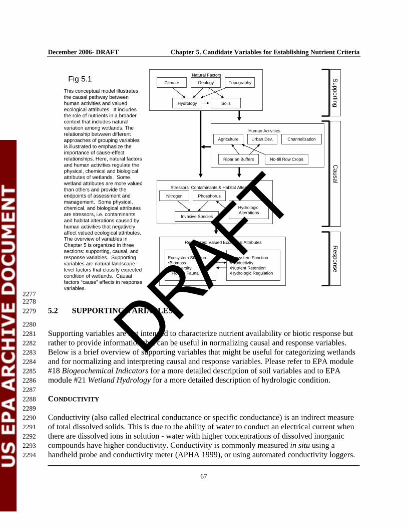
December 2006- DRAFT Chapter 5. Candidate Variables for Establishing Nutrient Criteria
67
Fig 5.1 Climate Geology
Soils
Topography
Hydrology
Agriculture Urban Dev.
No-till Row Crops
Channelization
Riparian Buffers
Nitrogen Phosphorus
Invasive Species
Hydrologic Alterations
Ecosystem Structure•Biomass•Biodiversity
Flora & Fauna
Ecosystem Function•Productivity•Nutrient Retention•Hydrologic Regulation
Human Activities
Natural Factors
Stressors: Contaminants & Habitat Alterations
Responses: Valued Ecological Attributes
Supporting
Causal
Response
This conceptual model illustrates the causal pathway between human activities and valued ecological attributes. It includes the role of nutrients in a broader context that includes natural variation among wetlands. The relationship between different approaches of grouping variables is illustrated to emphasize the importance of cause-effect relationships. Here, natural factors and human activities regulate the physical, chemical and biological attributes of wetlands. Some wetland attributes are more valued than others and provide the endpoints of assessment and management. Some physical, chemical, and biological attributes are stressors, i.e. contaminants and habitat alterations caused by human activities that negatively affect valued ecological attributes. The overview of variables in Chapter 5 is organized in three sections: supporting, causal, and response variables. Supporting variables are natural landscape-level factors that classify expected condition of wetlands. Causal factors “cause” effects in response variables.
2277 2278 5.2 SUPPORTING VARIABLES 2279
2280 Supporting variables are not intended to characterize nutrient availability or biotic response but 2281 rather to provide information that can be useful in normalizing causal and response variables. 2282 Below is a brief overview of supporting variables that might be useful for categorizing wetlands 2283 and for normalizing and interpreting causal and response variables. Please refer to EPA module 2284 #18 Biogeochemical Indicators for a more detailed description of soil variables and to EPA 2285 module #21 Wetland Hydrology for a more detailed description of hydrologic condition. 2286 2287 CONDUCTIVITY 2288 2289 Conductivity (also called electrical conductance or specific conductance) is an indirect measure 2290 of total dissolved solids. This is due to the ability of water to conduct an electrical current when 2291 there are dissolved ions in solution - water with higher concentrations of dissolved inorganic 2292 compounds have higher conductivity. Conductivity is commonly measured in situ using a 2293 handheld probe and conductivity meter (APHA 1999), or using automated conductivity loggers. 2294
DRAFT

December 2006- DRAFT Chapter 5. Candidate Variables for Establishing Nutrient Criteria
68
Because the conductivity changes with temperature, the raw measurement should be adjusted to 2295 a reference temperature of 25°C. A multiplier of 0.7 is commonly applied to estimate the total 2296 dissolved solids concentration (mg/L) in fresh water when the conductivity is measured in units 2297 of microSiemens per centimeter (μS/cm), although this multiplier varies with the types of 2298 dissolved ions and should be adjusted for local chemical conditions. 2299 2300 Conductivity is a useful tool for characterizing wetland inputs and interpreting nutrient condition 2301 because of its sensitivity to changes in these inputs. Rainfall tends to have lower conductivity 2302 than surface water, with ground water often having higher values due to the longer residence 2303 time of water in the subsurface. Coastal and marine waters – as well as water in terminal lakes 2304 and wetlands - have even higher conductivity due to the influence of salinity. Municipal and 2305 industrial discharges often have higher conductivity than their intake waters due to the addition 2306 of soluble wastes. Wetland hydrologic inputs can be identified by comparing the measured input 2307 conductivity with the conductivity of potential local sources. 2308 2309 SOIL PH 2310 2311 Soil pH can be important for categorizing wetland soils and interpreting soil nutrient variables. 2312 The pH of wetland soils and water varies over a wide range of values. Many ombrotrophic 2313 organic wetland soils (histosols) such as bogs, non-limestone based wetlands are often acidic and 2314 mineral wetland soils are frequently neutral or alkaline. Flooding a soil results in consumption of 2315 electrons and protons. In general, flooding acidic soils results in an increase in pH, and flooding 2316 alkaline soils decreases pH (Mitsch and Gosselink, 1993). The increase in pH of low pH (acidic) 2317 wetland soils is largely due to the reduction of iron and manganese oxides. However, the initial 2318 decrease in pH of alkaline wetland soils is due to rapid decomposition of soil organic matter and 2319 accumulation of CO2. The decrease in pH that generally occurs when alkaline soils are flooded 2320 results from the buildup of CO2 and carbonic acid. In addition, the pH of alkaline soils is highly 2321 sensitive to changes in the partial pressure of CO2. Carbonates of iron and manganese also can 2322 buffer the pH of soil to neutrality. Soil pH determinations should be made on wet soil samples. 2323 Once the soils are air-dried, oxidation of various reduced compounds results in decrease in pH 2324 and the values may not represent ambient conditions. 2325 2326 Soil pH is measured using commercially available combination electrodes on soil slurries. If air 2327 dry or moist soil is used, a 1:1 soil to water ratio should be used. For details on methodology, the 2328 reader is referred to Thomas (1996). 2329 2330 Soil pH can explain the availability and retention capacity of phosphorus. For example, 2331 phosphorus bioavailability is highest at soil pH near neutral conditions. For mineral soils, 2332 phosphorus adsorption capacity has been directly linked to extractable iron and aluminum. For 2333 details the reader is referred to Module-18 on Biogeochemical Indicators. 2334 2335
DRAFT
December 2006- DRAFT Chapter 5. Candidate Variables for Establishing Nutrient Criteria
69
SOIL BULK DENSITY 2336 2337 Soil bulk density is the mass of dry solids per unit volume of soil, which includes the volume of 2338 solids plus air- and water-filled pore space. Bulk density is a useful parameter for expressing the 2339 concentration of nutrients on a volume basis rather than mass basis. For example, concentration 2340 of nutrients in organic wetland soils can be high when expressed on a mass basis (mg/kg or μg/g 2341 of dry soil), as compared to mineral wetland soils. However, the difference in concentration may 2342 not be as high when expressed on a volume (cm3) basis, which is calculated as the product of 2343 bulk density and nutrient concentration per gram of soil. Expressing soil nutrient concentrations 2344 on a volume basis is especially relevant to uptake by vegetation since plant roots explore a 2345 specific volume, not mass, of soil. Expressing nutrients on a volume basis also helps in 2346 calculating total nutrient storage in a defined soil layer. 2347 2348 Bulk density is measured by collecting an intact soil core of known volume at specific depths in 2349 the soil (Blake and Hartge, 1986). Cores are oven-dried at 70oC and weighed. Bulk density is 2350 calculated as follows: 2351 2352 Bulk density (dry) (g/cm3) = mass dry weight (grams)/volume (cm3) 2353 2354 Bulk densities of wetland organic soils range from 0.1 to 0.5 g/cm3, whereas bulk densities of 2355 mineral wetland soils range from 0.5 to 1.5 g/cm3. Soil bulk densities are directly related to soil 2356 organic matter content, as bulk densities decrease with increase in soil organic matter content. 2357 2358 SOIL ORGANIC MATTER CONTENT 2359 2360 Soil organic matter can be important for categorizing wetland soils and interpreting soil nutrient 2361 variables. Wetland soils often are characterized by the accumulation of organic matter because 2362 rates of primary production often exceed rates of decomposition. Some wetlands accumulate 2363 thick layers of organic matter that, over time, form peat soil. Organic matter provides nutrient 2364 storage and supply, increases the cation exchange capacity of soils, enhances adsorption or 2365 deactivation of organic chemicals and trace metals, and improves overall soil structure, which 2366 results in improved air and water movement. A number of methods are now routinely used to 2367 estimate soil organic matter content expressed as total organic carbon or loss on ignition (APHA, 2368 1999; Nelson and Sommers, 1996). 2369 2370 Soil organic matter content represents the soil organic carbon content of soils. Typically, soil 2371 organic matter content is approximately 1.7 to 1.8 times that of total organic carbon. The carbon 2372 to nitrogen and carbon to phosphorus ratios of soils can provide an indication of nutrient 2373 availability in soils. 2374
DRAFT

December 2006- DRAFT Chapter 5. Candidate Variables for Establishing Nutrient Criteria
70
2375 HYDROLOGIC CONDITION 2376 2377 Wetland hydrologic condition is important for characterizing wetlands and for normalizing many 2378 causal and response variables. Hydrologic conditions can directly affect the chemical and 2379 physical processes governing nutrient and suspended solids dynamics within wetlands (Mitsch 2380 and Gosselink, 2000). Detailed, site-specific hydrologic information available is best, but at a 2381 minimum, some estimate of water level fluctuation should be made. A defining characteristic of 2382 wetlands is oxygen deficiency in the soil caused by flooding or soil saturation. These conditions 2383 influence vegetation dynamics through differential growth and survival of plant species and also 2384 exert significant control over biogeochemical processes involved in carbon flow and nutrient 2385 cycling within wetlands. Spatial and temporal patterns in hydrology can create complex patterns 2386 in soil and water column oxygen availability including alternating aerobic and anaerobic 2387 conditions in wetland soils, with obvious implications for plant response and biogeochemical 2388 process dynamics. Water levels in wetlands can be determined using a staff gauge when surface 2389 water is present. A staff gauge measures the depth of surface flooding relative to a reference 2390 point such as the soil surface. While surface flooding may be rare or absent in many wetlands, 2391 high water tables may still cause soil saturation in the rooting zone. In wetlands where soils are 2392 saturated, water level can be measured with a small diameter perforated tube installed in the soil 2393 to a specified depth (Amoozegar and Warrick 1986). Automated water level recorders using 2394 floats, capacitance probes, or pressure transducers are suitable for measuring water levels both 2395 above- and below-ground. 2396 2397 2398 5.3 CAUSAL VARIABLES 2399
Causal variables are intended to characterize nutrient availability in wetlands. Most wetlands are 2400 characterized by extremely variable nutrient loading rates and close coupling of soil and water 2401 column processes. As a result, estimates of nutrient loading and measurements of soil nutrients 2402 may prove more useful than direct measurements of water column nutrient concentrations as 2403 causal variables for establishing the nutrient condition of wetlands. Nutrient loading history and 2404 soil nutrient measures can integrate a wetland’s variable nutrient history over a period of years 2405 and may provide especially useful metrics against which to evaluate nutrient condition. Wetlands 2406 exhibit a high degree of spatial heterogeneity in chemical composition of soil layers, and areas 2407 impacted by nutrients may exhibit more variability than unimpacted areas of the same wetland. 2408 Thus, sampling protocols should capture this spatial variability. Developing nutrient criteria and 2409 monitoring the success of nutrient management programs involves important considerations for 2410 sampling designed to capture spatial and temporal patterns. (See Study Design Module and the 2411 Biogeochemical Indicators Module.) 2412 2413 Below is a brief overview of the use of nutrient loading and soil and water column nutrient 2414 measures for estimating nutrient condition of wetlands. Please refer to the EPA module #19 2415 Nutrient Loading Models for a detailed description of nutrient load estimation and to EPA 2416
DRAFT
December 2006- DRAFT Chapter 5. Candidate Variables for Establishing Nutrient Criteria
71
module #18 Biogeochemical Indicators for a more detailed description of soil and water column 2417 nutrient measures. 2418 2419 NUTRIENT LOADING 2420 2421 External nutrient loads to wetlands are determined primarily by surface and subsurface transport 2422 from the contributing landscape, and vary significantly as a function of weather and landscape 2423 characteristics such as soils, topography, and land use. Most wetlands are characterized by 2424 extremely variable hydrologic and nutrient loading rates, which present considerable obstacles to 2425 obtaining adequate direct measurement of nutrient inputs. Adequate measurement of loads may 2426 require automated samplers capable of providing flow-weighted samples when loading rates are 2427 highly variable. In many cases, non-point source loads simply may not be adequately sampled. 2428 The more detailed the loading measurements the better, but it is not reasonable to expect 2429 adequate direct measurement of loads for most wetlands. In the absence of sufficient, direct 2430 measurements, it may be possible to estimate nutrient loading using an appropriate loading 2431 model or at least to provide a relative ranking of wetlands based on expected nutrient load. One 2432 advantage of loading models is that nutrient loading can be integrated over the appropriate time 2433 scale for characterizing wetland nutrient condition and, in some cases, historical loading patterns 2434 can be reconstructed. Loading models also can provide hydrologic loading rates to calculate 2435 critical supporting variables such as hydroperiod and residence times. 2436 2437 Loading function models are based on empirical or semi-empirical relationships that provide 2438 estimates of pollutant loads on the basis of long-term measurements of flow and contaminant 2439 concentration. Generally, loading function models contain procedures for estimating pollutant 2440 load based on empirical relationships between landscape physiographic characteristics and 2441 phenomena that control pollutant export. McElroy et al. (1976) and Mills (1985) described 2442 loading functions employed in screening models developed by the USEPA to facilitate 2443 estimation of nutrient loads from point and nonpoint sources. The models contain simple 2444 empirical expressions that relate the magnitude of nonpoint pollutant load to readily available or 2445 measurable input parameters such as soils, land use and land cover, land management practices, 2446 and topography. Preston and Brakebill (1999) described a spatial regression model that relates 2447 the water quality conditions within a watershed to sources of nutrients and to those factors that 2448 influence transport of the nutrients. The regression model, Spatially-Referenced Regressions on 2449 Watersheds (SPARROW) involves a statistical technique that utilizes spatially referenced 2450 information and data to provide estimates of nutrient load (Smith et al., 1997; Smith et al., 2003; 2451 http://water.usgs.gov/nawqa/sparrow/). 2452 2453 In general, the SPARROW methodology was designed to provide statistically based 2454 relationships between stream water quality and anthropogenic factors such as contaminant 2455 sources within the contributing watersheds, land surface characteristics that influence the 2456 delivery of pollutants to the stream, and in-stream contaminant losses via chemical and 2457 biological process pathways. The Generalized Watershed Loading Functions (GWLF) model 2458
DRAFT

December 2006- DRAFT Chapter 5. Candidate Variables for Establishing Nutrient Criteria
72
(Haith and Shoemaker, 1987; Haith et al., 1992) uses daily time steps, and to some extent, both 2459 can be used to examine seasonal variability and the response to landscape characteristics of 2460 specific watersheds. The GWLF model was developed to evaluate the point and non-point 2461 loading of nitrogen and phosphorus in urban and rural watersheds. The model enhances 2462 assessment of effectiveness of certain land use management practices and makes extensive use of 2463 readily available watershed data. The GWLF also provides an analytical tool to identify and rank 2464 critical areas of a watershed and to evaluate alternative land management programs. 2465 2466 Process-oriented simulation models attempt to explicitly represent biological, chemical, and 2467 physical processes controlling hydrology and pollutant transport. These models are at least partly 2468 mechanistic in nature and are built from equations that contain directly definable, observable 2469 parameters. Examples of process-oriented simulation models that have been used to predict 2470 watershed hydrology and water quality include the Agricultural Nonpoint Source model 2471 (AGNPS), the Hydrologic Simulation Program-Fortran (HSPF), and the Soil and Water 2472 Assessment Tool (SWAT). AGNPS (Young et al.1987) is a distributed parameter, event-based 2473 and continuous simulation model that predicts the behavior of runoff, sediment, nutrients and 2474 pesticide transport from watersheds that have agriculture as the primary land use. Because of its 2475 simplicity and ease of use, AGNPS is probably one of the most widely used hydrologic and 2476 water quality models of watershed assessment. HSPF (Johansen et al., 1984; Bicknell et al., 2477 1993; Donigian et al., 1995a) is a lumped parameter, continuous simulation model developed 2478 during the mid-1970’s to predict watershed hydrology and water quality for both conventional 2479 and toxic organic pollutants. HSPF is one of the most comprehensive models available for 2480 simulating non-point source nutrient loading. The capability, strengths, and weaknesses of HSPF 2481 have been demonstrated by its application to many urban and rural watersheds and basins (e.g., 2482 Donigian et al., 1990; Moore et al., 1992; and Ball et al., 1993). SWAT (Arnold et al., 1995) is a 2483 lumped parameter, continuous simulation model developed by the USDA-Agricultural Research 2484 Services that provides long-term simulation of impact of land management practices on water, 2485 sediment, and agricultural chemical yields in large complex watersheds. Because of its lumped 2486 parameter nature, coupled with its extensive climatic, soil, and management databases, the 2487 SWAT model is one of the most widely used hydrologic and water quality models for large 2488 watersheds and basins, and the model has found widespread application in many modeling 2489 studies that involve systemic evaluation of impact of agricultural management on water quality. 2490 2491 These loading models address only gross, external nutrient inputs. It is important to consider the 2492 overall mass balance for the receiving wetland in developing measures of nutrient loading 2493 against which to evaluate wetland nutrient condition. This requires some estimate of nutrient 2494 export, storage, and transformation. In the absence of sufficient, direct measurements from 2495 which to calculate nutrient mass balance, it may be possible to estimate nutrient mass balances 2496 using an appropriate wetland model. Strictly empirical, regression models can be used to 2497 estimate nutrient retention and export in wetlands but these regressions are of little value outside 2498 the data domain in which they are developed. When developed for a diverse set of systems, the 2499 scatter in these regressions can be quite large. In contrast to strictly empirical regressions, mass 2500
DRAFT
December 2006- DRAFT Chapter 5. Candidate Variables for Establishing Nutrient Criteria
73
balance models incorporate principles of mass conservation. These models integrate external 2501 loading to the wetland, nutrient transformation and retention within the wetland, and nutrient 2502 export from the wetland. Mass balance models allow time varying hydrologic and nutrient inputs 2503 and can provide estimates of spatial nutrient distribution with the wetland. The most difficult 2504 problem is developing removal rate equations which adequately represent nutrient 2505 transformation and retention across the range of conditions for which estimates are needed. 2506 2507 LAND USE 2508 2509 Identifying land uses in regions surrounding wetlands are important for characterizing reference 2510 condition, identifying reference wetlands, and providing indicators of nutrient loading rates for 2511 criteria development. Most simply, the percentage of natural area, or the percentage of 2512 agricultural and urban lands can be used to characterize land uses around wetlands. More 2513 detailed quantitative data can be gathered from GIS analyses which provides higher resolution 2514 identification of land use types, such as pastures, row crops, and confined animal feeding 2515 operations for agriculture. Ideally these characterizations should be done for the entire 2516 sourceshed, including both air and water, in the regions around wetlands. Air-sheds should 2517 incorporate potential atmospheric sources of nutrients, and watersheds should incorporate 2518 potential aquatic sources. However, in practice, land use around wetlands is typically used for 2519 defining reference wetlands and is used in most nutrient loading models to characterize 2520 groundwater and surface water sources. Land use in buffer zones, one kilometer zones around 2521 wetlands and wetland watersheds (delineated by elevation) have been used to characterize 2522 human activities that could be affecting wetlands. 2523 2524 EXTRACTABLE SOIL NITROGEN AND PHOSPHORUS 2525 2526 Ammonium is the dominant form of inorganic N in wetland soils, and unlike total soil N (Craft 2527 et al. 1995, Chiang et al. 2000), soil extractable NH4-N increases in response to N loadings. 2528 Enrichment leads to enhanced cycling of N between wetland biota (Valiela and Teal 1974, 2529 Broome et al. 1975, Chalmers 1979, Shaver et al. 1998), greater activity of denitrifying bacteria 2530 (Johnston 1991, Groffman 1994, White and Reddy 1999) and accelerated organic matter and N 2531 accumulation in soil (Reddy et al. 1993, Craft and Richardson 1998). In most cases, extractable 2532 soil N should be measured in the surface soil where roots and biological activity are 2533 concentrated. 2534 2535 Extractable N is measured by extraction of inorganic (NH4-N) N with 2 M KCl (Mulvaney 2536 1996). Ten to twenty grams of field moist soil is equilibrated with 100 ml of 2 M KCl for one 2537 hour on a reciprocating shaker followed by filtration through Whatman No. 42 filter paper. 2538 Ammonium-N in soil extracts is determined colorimetrically using the phenate or salicylate 2539 method (APHA 1999, Method 350.2, USEPA, 1993a). 2540 2541
DRAFT
December 2006- DRAFT Chapter 5. Candidate Variables for Establishing Nutrient Criteria
74
Extractable P often is a reliable indicator of the P enrichment of soils, and in wetlands, 2542 extractable P is strongly correlated with surface water P concentration and P enrichment from 2543 external sources (Reddy et al. 1995, 1998). Selected methods used to extract P are described 2544 below (Kuo 1996). Many soil testing laboratories perform these analyses on a routine basis. 2545 Historically, these methods have been used to determine nutrient needs of agronomic crops, but 2546 the methods have been used more recently to estimate P impacts in upland and wetland soils 2547 (Sharpley et al. 1992; Nair et al. 1995; Reddy et al. 1995; 1998). 2548 2549 The Mehlich I method is typically used in Southeast and Mid-Atlantic region on mineral soils 2550 with pH of < 7.0 (Kuo 1996). The extractant consists of dilute concentrations of strong acids. 2551 Many plant nutrients such as P, K, Ca, Mg, Fe, Zn, and Cu extracted with Mehlich I methods 2552 have been calibrated for production of crops in agricultural ecosystems. This solvent extracts 2553 some Fe and Al- bound P, and some Ca-bound P. Soil (dry) to extractant ratio is set at 1: 4, for 2554 mineral soils, while wider ratios are used for organic soils. Soil solutions are equilibrated for 2555 period of 5 minutes on a mechanical shaker and filtered through Whatman No. 42 filter. Filtered 2556 solutions are analyzed for P and other nutrients using standard methods (Method 365. 1, USEPA, 2557 1993a). 2558 2559 The Bray P-1 method has been widely used as an index of available P in soils (Kuo 1996). The 2560 combination of dilute concentration of strong acid (HCl at 0.025 M) and ammonium fluoride 2561 (NH4F at 0.03 M) is designed to remove easily acid extractable soluble P forms such as Ca-2562 bound P, and some Fe and Al-bound P. Soil (dry) to extractant ratio is set at 1: 7 for mineral soils 2563 with wider ratios used for highly organic soils, then shaken for 5 minutes and filtered through 2564 Whatman No. 42 filter. Filtered solutions are analyzed for P and other nutrients using the same 2565 methods used for the Mehlich I extraction (Method 365. 1, USEPA 1993a). 2566 2567 Bicarbonate Extractable P is a suitable method for calcareous soils. Soil P is extracted from the 2568 soil with 0.5 M NaHCO3, at nearly a constant pH of 8.5 (Kuo 1996). In calcareous, alkaline, or 2569 neutral soils containing Ca-bound P, this extractant decreases the concentration of Ca in solution 2570 by causing precipitation of Ca as CaCO3 ; and as result P concentration in soil solution increases. 2571 Soil (dry) to extraction ratio is set at 1: 20 for mineral soils and 1:100 for highly organic soils. 2572 Soil solutions are equilibrated for period of 30 minutes on a shaker and filtered through 2573 Whatman No. 42 filter paper and analyzed for P using standard methods (Method 365. 1, 2574 USEPA, 1993a). 2575 2576 TOTAL SOIL NITROGEN AND PHOSPHORUS 2577 2578 Nutrient enrichment leads to enrichment of total soil P (Craft and Richardson 1993, Reddy et al. 2579 1993, Bridgham et al., 2001). In contrast, soil total N usually does not increase in response to 2580 nutrient enrichment (Craft et al. 1995, Chiang et al. 2000). Rather, enrichment leads to enhanced 2581 cycling of N between wetland biota that is reflected in greater N uptake and net primary 2582 production (NPP) of wetland vegetation (Valiela and Teal 1974, Broome et al. 1975, Chalmers 2583
DRAFT

December 2006- DRAFT Chapter 5. Candidate Variables for Establishing Nutrient Criteria
75
1979, Shaver et al. 1998), greater activity of denitrifying bacteria (Johnston 1991, Groffman 2584 1994, White and Reddy 1999) and accelerated organic matter and N accumulation in soil (Reddy 2585 et al. 1993, Craft and Richardson 1998). In most cases, total N and P should be measured in at 2586 least the surface soil where most roots and biological activity are concentrated. 2587 2588 Since ammonium N is the dominant form of inorganic nitrogen in saturated wetland soils with 2589 very little nitrate (NO3) present, total Kjeldahl nitrogen (TKN) can generally be taken as a 2590 measure of total N in such soils. The difference between TKN and ammonium N provides 2591 information on soil organic N. The soil organic carbon to soil organic nitrogen ratio of soils can 2592 provide an indication soils capacity to mineralize organic N and provide ammonium N to 2593 vegetation. TKN in soils is determined by converting organic forms of N to NH4-N by digestion 2594 with concentrated H2SO4 at temperatures of 300-350 o C (Bremner 1996). The NH4-N in digested 2595 samples is analyzed using colorimetric (e.g., phenate, salicylate) methods (APHA 1999, 2596 Mulvaney 1996). 2597 2598 Total P in soils is determined by oxidation of organic forms of P and acid (nitric-perchloric acid) 2599 dissolution of minerals at temperatures of <300oC (Kuo 1996). Digested solutions are analyzed 2600 for P using colorimetric methods (e.g., ascorbic acid-molybdate) (APHA 1999, Kuo 1996). 2601 Many laboratories may not have access to perchloric acid fume-hoods. Alternatively, soil total 2602 phosphorus can be determined using ashing method (Anderson, 1976). Results obtained from 2603 this method are reliable and comparable to total phosphorus measurements made using 2604 perchloric acid digestion method. 2605 2606 WATER COLUMN NITROGEN AND PHOSPHOROUS 2607 2608 Nutrient inputs to wetlands are highly variable across space and time, however, so that single 2609 measurements of water column N and P represent only a “snap-shot” of nutrient condition, and 2610 may or may not reflect the long-term pattern of nutrient inputs that alter biogeochemical cycles 2611 and affect wetland biota. The best use of water column N and P concentrations for nutrient 2612 criteria development will be based on frequent monitoring of nutrient concentrations over time 2613 (e.g., weekly or monthly measurements). Of course, in wetlands that are seldom flooded, 2614 measurements of water column N and P may not be practical or even relevant for assessing 2615 impacts. Whenever, water samples are obtained, it is important the water depth is recorded, as 2616 nutrient concentration is related to water depth. In the case of tidal estuarine or freshwater 2617 wetlands, it is also important to record flow and the point in the tidal cycle that the samples were 2618 collected. 2619 2620 Methodologies to monitor N in surface waters are well developed for other ecosystems and can 2621 be readily adopted for wetlands. The most commonly monitored N species are total Kjeldahl 2622 nitrogen (TKN), ammonium N, and nitrate plus nitrite N (APHA 1999). The TKN analysis 2623 includes both organic and ammonium N, but does not include nitrate plus nitrite N. Organic N is 2624 determined as the difference between TKN and NH4-N. Forms of N in surface water are 2625
DRAFT
December 2006- DRAFT Chapter 5. Candidate Variables for Establishing Nutrient Criteria
76
measured by standard methods, including phenol-hypochlorite for ammonium N, cadmium 2626 reduction of nitrate to nitrite for nitrate N and Kjeldahl digestion of total N to ammonium for 2627 analysis of total N (APHA 1999). Dissolved organic N is primarily used by heterotrophic 2628 microbes whereas plants and various microorganisms take up inorganic forms of N (ammonium 2629 N and nitrate N) to support metabolism and new growth. 2630 2631 Methodologies to monitor P in surface waters are well developed for aquatic ecosystems and can 2632 be readily adopted for wetlands (APHA 1999). The most commonly measured forms of P in 2633 surface water are total P, dissolved inorganic P (i.e., PO4-P), and total dissolved P. To trace the 2634 transport and transformations of P in wetlands, it might be useful to distinguish four forms of P: 2635 (i) dissolved inorganic P (DIP, also referred to as dissolved reactive P (DRP) or soluble reactive 2636 phosphorous (SRP)); (ii) dissolved organic P (DOP); (iii) particulate inorganic P (PIP), and (iv) 2637 particulate organic P (POP). Dissolved inorganic P (PO4-P) is considered bioavailable (e.g., 2638 available for uptake and use by microorganisms, algae and vegetation) whereas organic and 2639 particulate P forms generally must be transformed into inorganic forms before being considered 2640 bioavailable. In P limited wetlands, a significant fraction of DOP can be hydrolyzed by 2641 phosphatases and utilized by both bacteria, algae, and macrophytes. 2642 2643 2644 5.4 RESPONSE VARIABLES 2645
2646 Biotic measures that can integrate a wetland’s variable nutrient history over a period of months 2647 to years may provide the most useful measures of wetland response to nutrient enrichment. 2648 Microorganisms, algae and macrophytes respond to nutrient enrichment by (1) increasing the 2649 concentration of nutrients (P, N) in their tissues, (2) increasing growth and biomass production 2650 and (3) shifts in species composition. The biotic response to nutrient enrichment generally occurs 2651 in a sequential manner as nutrient uptake occurs first, followed by increased biomass production 2652 followed by a shift in species composition as some species disappear and other species replace 2653 them. Macroinvertebrates respond to nutrient enrichment indirectly as a result of changes in food 2654 sources, habitat structure, and dissolved oxygen. Because of their short life cycle, 2655 microorganisms and algae respond more quickly to nutrient enrichment than macrophytes. 2656 However, biotic measures that can integrate a wetland’s variable nutrient history over a period of 2657 months to years may provide the most useful measures of wetland response. 2658 2659 Below is a brief overview of the use of macrophytes, algae, and macroinvertebrates to assess 2660 nutrient condition of wetlands. Please refer to the relevant modules in the EPA series “Methods 2661 for Evaluating Wetland Condition” for details on using vegetation 2662 (http://www.epa.gov/waterscience/criteria/wetlands/16Indicators.pdf ; 2663
DRAFT
December 2006- DRAFT Chapter 5. Candidate Variables for Establishing Nutrient Criteria
77
http://www.epa.gov/waterscience/criteria/wetlands/10Vegetation.pdf), algae 2664 (http://www.epa.gov/waterscience/criteria/wetlands/11Algae.pdf), and macroinvertebrates 2665 (http://www.epa.gov/waterscience/criteria/wetlands/9Invertebrate.pdf). to assess wetland 2666 condition., including nutrients. 2667 2668 MACROPHYTE NITROGEN AND PHOSPHORUS 2669 2670 Wetland macrophytes respond to nutrient enrichment by increasing uptake and storage of N and 2671 P (Verhoeven and Schmitz 1991, Shaver et al. 1998, Chiang et al. 2000). In wetlands where P is 2672 the primary limiting nutrient, the P content of vegetation increases almost immediately (within a 2673 few months) in response to nutrient enrichment (Craft et al. 1995). Increased P uptake by plants 2674 is known as “luxury uptake” because P is stored in vacuoles and used later (Davis 1991). Like P, 2675 leaf tissue N may increase in response to N enrichment (Brinson et al. 1984, Shaver et al. 1998). 2676 However, most N is directly used to support new plant growth so that luxury uptake of N is not 2677 usually observed (Verhoeven and Schmitz 1991). Tidal marsh grasses, however do appear to 2678 store nitrogen in both living and dead tissues that can be accessed by living plant tissue. A 2679 discussion of conservation and translocation of N in saltwater tidal marshes can be found in 2680 Hopkinson and Schubauer 1980, and in Thomas and Christian 2001. 2681 2682 Nutrient content of macrophyte tissue holds promise as a means to assess nutrient enrichment of 2683 wetlands. However, several caveats should be kept in mind when using this diagnostic tool 2684 (Gerloff 1969, Gerloff and Krombholz 1966, EPA 2002c). 2685 2686 1. The most appropriate plant parts to sample and analyze should be determined. It is 2687
generally recognized that the plant or plant parts should be of the same physiological age. 2688 2689 2. Samples from the same species should be collected and analyzed. Different species 2690
assimilate and concentrate nutrients to different levels. 2691 2692 3. Tissue nutrient concentrations vary with (leaf) position, plant part and age. It is important 2693
to sample and analyze leaves from the same position and age (e.g., third leaf from the 2694 terminal bud on the plant) to ensure comparability of results from sampling of different 2695 wetlands. 2696
2697 4. Tissue P may be a more reliable indicator of nutrient condition than N. This is because N 2698
is used to increase production of aboveground biomass whereas excess P is stored via 2699 luxury uptake. 2700
2701 Another promising macrophyte-based tool is the measurement of nutrient resorption of N and P 2702 prior to leaf senescence and dieback. Nutrient resorption is an important strategy used by 2703 macrophytes to conserve nutrients (Hopkinson and Schubauer 1984; Shaver and Melillo 1984). 2704 In nutrient-poor environments, macrophytes resorb N and P from green leaves prior to 2705
DRAFT
December 2006- DRAFT Chapter 5. Candidate Variables for Establishing Nutrient Criteria
78
senescence, leading to low concentrations of N and P in senesced leaves. In nutrient-rich 2706 environments, resorption becomes less important so that senesced leaves retain much of the N 2707 and P that was present when the leaves were green. 2708 2709 Nitrogen and phosphorus should be measured in green leaves of the same approximate age 2710 collected from the dominant wetland plant species. Samples also should be collected throughout 2711 the wetland to account for spatial variability. If an environmental gradient is known or suspected 2712 to exist within the wetland, then sites along this gradient should be sampled separately. At each 2713 sampling location, approximately five green leaves are collected from each of dominant plant 2714 species. Leaves are collected from the middle portion of the stem, avoiding very young leaves at 2715 the top of the stem and very old leaves at the bottom of the stem. At each location, leaf samples, 2716 by species, are combined for analysis, oven-dried at 70oC and ground. 2717 2718 Nitrogen is measured by dry combustion using a CHN analyzer. Phosphorus is measured 2719 colorimetrically after digestion in strong acid (H2SO4-H2O2) (Allen et al. 1986). Many land-grant 2720 universities, state agricultural testing laboratories, and environmental consulting laboratories 2721 perform these analyses. Contact your local U.S. Department of Agriculture office or land-grant 2722 agricultural extension office for information on laboratories that perform plant tissue nutrient 2723 analyses. 2724 2725 Please see the EPA module 16, Vegetation-based Indicators of Wetland Nutrient Enrichment 2726 (http://www.epa.gov/waterscience/criteria/wetlands/16Indicators.pdf) for a detailed description 2727 of indicators derived from to N and P content of macrophytes. 2728 2729 ABOVEGROUND BIOMASS AND STEM HEIGHT 2730 2731 Wetland macrophytes also respond to nutrient enrichment by increased net primary production 2732 (NPP) and growth if other factors such as light are not limiting growth (Chiang et al. 2000). Net 2733 primary production is the amount of carbon fixed during photosynthesis that is incorporated into 2734 new leaves, stems and roots. Most techniques to measure NPP focus on aboveground biomass 2735 and discount root production because it is difficult to measure even though root production may 2736 account for 50% of NPP. The simplest way to measure aboveground biomass is by harvesting all 2737 of the standing material (biomass) at the end of the growing season (Broome et al., 1986). The 2738 harvest method is useful for measuring NPP of herbaceous emergent vegetation, especially in 2739 temperate climates where there is a distinct growing season. If root production desired, it can be 2740 determined by sequentially harvesting roots at monthly intervals during the year (Valiela et. al, 2741 1976). 2742 2743 Enhanced NPP often is reflected by increased height and, sometimes, stem density of herbaceous 2744 emergent vegetation (Broome et al 1983). Increased stem density, however, may reflect other 2745 factors like vigorous clonal growth so it is not recommended as an indicator of nutrient 2746 enrichment. 2747
DRAFT
December 2006- DRAFT Chapter 5. Candidate Variables for Establishing Nutrient Criteria
79
2748 Aboveground biomass of herbaceous vegetation may be determined by end-of-season harvest of 2749 aboveground plant material in small 0.25 m2 quadrats stratified by macrophyte species or 2750 inundation zone (Broome et al. 1986). Stem height of individuals of dominant species is 2751 measured in each plot. Height of the 5 to 10 tallest stems in each plot has been shown to be a 2752 reliable indicator of NPP (Broome et al. 1986) that saves time as compared to height 2753 measurements of all stems in the plot. Aboveground biomass is clipped at the end of the growing 2754 season, in late summer or fall. Clipped material is separated into live (biomass) versus dead 2755 material then dried at 70oC to a constant weight. For stem height and biomass sampling, 5 to 10 2756 plots per vegetation zone are collected. In forested sites, biomass production is defined as the 2757 sum of the leaf and fruit fall and aboveground wood production (Newbould, 1967). Please see 2758 the EPA module Vegetation-based Indicators of Wetland Nutrient Enrichment 2759 (http://www.epa.gov/waterscience/criteria/wetlands/16Indicators.pdf ) for a detailed description 2760 for sampling aboveground biomass in wetlands. 2761 2762 ALGAL NITROGEN & PHOSPHORUS 2763 2764 In some cases, measurements of algal N and P can provide a useful complement to vegetation 2765 and soil nutrient analyses that integrate nutrient history over a period of months in the case of 2766 vegetation (Craft et al. 1995) to years in the case of soils (Craft and Richardson 1998, Chiang et 2767 al. 2000). Nutrient concentrations in algae can integrate variation in water column N and P 2768 bioavailability over a time scale of weeks, potentially providing an indication of the recent 2769 nutrient status of a wetland (Fong et al., 1990; Stevenson et al. 2001; ). Caution is warranted for 2770 this method because it is not useful in all wetlands, for example in wetlands where surface 2771 inundation occurs intermittently or for short periods of time, where the water surface is severely 2772 shaded as in some forested wetlands, or under other circumstances where unrelated 2773 environmental factors exert primary control over algal growth. 2774 2775 Algae should be sampled by collecting grab samples from different locations in the wetland to 2776 account for spatial variability in the wetland. If an environmental gradient is known or suspected 2777 (i.e., decreasing canopy or impacted land uses), or exists within the wetland as a result of 2778 specific source discharges, then sites along this gradient should be sampled separately. 2779 Comparisons among wetlands or locations within a wetland should be done on a habitat-specific 2780 basis (e.g.,phytoplankton versus periphyton). Samples are processed in the same manner as 2781 wetland plants to determine N and P content. Nitrogen is determined using a CHN analyzer 2782 whereas P is measured colorimetrically after acid digestion. 2783 2784 Please see the EPA module Using Algae to Assess Environmental Conditions in Wetlands 2785 (http://www.epa.gov/waterscience/criteria/wetlands/11Algae.pdf) for a detailed description of 2786 indicators derived from to N and P content of algae. 2787 2788 MACROPHYTE COMMUNITY STRUCTURE AND COMPOSITION 2789
DRAFT
December 2006- DRAFT Chapter 5. Candidate Variables for Establishing Nutrient Criteria
80
2790 The composition of the plant community and the changes that result from human activities can 2791 be used as sensitive indicators of the biological integrity of wetland ecosystems. In particular, 2792 aggressive, fast-growing species such as cattail (Typha spp.), giant reed (Phragmites communis) 2793 reed canarygrass (Phalaris arundincea) and other clonal species invade and may eventually 2794 come to dominate the macrophyte community. Data collection methods and analyses for using 2795 macrophyte community structure and composition as an indicator of nutrient enrichment and 2796 ecosystem integrity for wetlands are described in Vegetation-based Indicators of Wetland 2797 Nutrient Enrichment (http://www.epa.gov/waterscience/criteria/wetlands/16Indicators.pdf ) and 2798 Using Vegetation to Assess Environmental Conditions in Wetlands 2799 (http://www.epa.gov/waterscience/criteria/wetlands/10Vegetation.pdf), respectively. 2800 2801 ALGAL COMMUNITY STRUCTURE AND COMPOSITION 2802 2803 Algae can be used as a valuable indicator of biological and ecological condition of wetlands. 2804 Structural and functional attributes of algae can be measured including diversity, biomass, 2805 chemical composition, productivity, and other metabolic functions. Species composition of 2806 algae, particularly of the diatoms, is commonly used as an indicator of biological integrity and 2807 physical and chemical conditions of wetlands. Discussions of sampling, data analyses, and 2808 interpretation are included in Using Algae to Assess Environmental Conditions in Wetlands 2809 (http://www.epa.gov/waterscience/criteria/wetlands/11Algae.pdf). 2810 2811 INVERTEBRATE COMMUNITY STRUCTURE AND COMPOSITION 2812 2813 Aquatic invertebrates can be used to assess the biological and ecological condition of wetlands. 2814 The approach for developing an Index of Biological Integrity (IBI) for wetlands based on aquatic 2815 invertebrates is described in Developing an Invertebrate Index of Biological Integrity for 2816 Wetlands (http://www.epa.gov/waterscience/criteria/wetlands/9Invertebrate.pdf). 2817 2818 SUMMARY 2819 2820 Candidate variables to use in determining nutrient condition of wetlands and to help identify 2821 appropriate nutrient criteria for wetlands consist of supporting variables, causal variables, and 2822 response variables. Supporting variables provide information useful in normalizing causal and 2823 response variables and categorizing wetlands. Causal variables are intended to characterize 2824 nutrient availability (or assimilation) in wetlands and could include nutrient loading rates and 2825 soil nutrient concentrations. Response variables are intended to characterize biotic response and 2826 could include community structure and composition of macrophytes and algae. 2827 2828 The complex temporal and spatial structure of wetlands will influence the selection of variables 2829 to measure and methods for measuring them. The information contained in this chapter is a brief 2830 summary of suggested analyses that can be used to determine wetland condition with respect to 2831
DRAFT

December 2006- DRAFT Chapter 5. Candidate Variables for Establishing Nutrient Criteria
81
nutrient status. The authors recognize that the candidate variables and analytical methods 2832 described here will generally be the most useful to identifying wetland nutrient condition, other 2833 methods and analyses may be more appropriate in certain systems. 2834 2835
DRAFT

December 2006 – DRAFT Chapter 6. Database Development and New Data Collection
82
Chapter 6 Database Development and New Data 2836
Collection 2837
2838 6.1 INTRODUCTION 2839
2840 A database of relevant water quality information can be an invaluable tool to States and Tribes as 2841 they develop nutrient criteria. In some cases existing data are available and can provide 2842 additional information that is specific to the region where criteria are to be set. However, little or 2843 no data are available for most regions or parameters, and creating a database of newly gathered 2844 data is strongly recommended. In the case of existing data, the data should be located, and their 2845 suitability (type and quality and sufficient associated metadata) ascertained. It is also important 2846 to determine how the data were collected to ensure that future monitoring efforts are compatible 2847 with earlier approaches. 2848 2849 Databases operate much like spreadsheet applications, but have greater capabilities. Databases 2850 store and manage large quantities of data and allow viewing and exporting of data sorted in a 2851 variety of ways, while spreadsheets analyze and graphically display small quantities of data. 2852 Databases can be used to organize existing information, store newly gathered monitoring data, 2853 and manipulate data for water quality criteria development. Databases can sort data for export 2854 into statistical analyses programs, spreadsheets, and graphics programs. This chapter will discuss 2855 the role of databases in nutrient criteria development, and provide a brief review of existing 2856 sources of nutrient-related water quality information for wetlands. 2857 2858 2859 6.2 DATABASES AND DATABASE MANAGEMENT 2860
A database is a collection of information related to a particular subject or purpose. Databases are 2861 arranged so that individual values are kept separate, yet can be linked to other values based on 2862 some common denominator (such as association of time or location). Geographic Information 2863 Systems (GIS) are geo-referenced relational databases that have a geographical component (i.e., 2864 spatial platform) in the user interface. Spatial platforms associated with a database allow 2865 geographical display of sets of sorted data. GIS platforms such as ArcView™, ArcInfo™, and 2866 MapInfo™ are frequently used to integrate spatial data with monitoring data for watershed 2867 analysis. Data stored in simple tables, relational database or geo-reference databases can also be 2868 located, retrieved and manipulated using queries. A query allows the user to find and retrieve 2869 only the data that meets user-specified conditions. Queries can also be used to update or delete 2870 multiple records simultaneously and to perform built-in or custom calculations of data. Data in 2871 tables can be analyzed and printed in specific layouts using reports. Data can be analyzed or 2872 presented in a specific way in print by creating a report. The most effective use of these tools 2873 requires a certain amount of training, expertise, and software support, especially when using geo-2874 referenced data. 2875
DRAFT

December 2006 – DRAFT Chapter 6. Database Development and New Data Collection
83
2876 To facilitate data storage, manipulation and calculations, it is highly recommended that historical 2877 and present-day data be transferred to a relational database (i.e., Access™). Relational 2878 databases store data in tables as sets of rows and columns, and are powerful tools for data 2879 manipulation and initial data reduction. They allow selection of data by specific, multiple 2880 criteria, and definition and redefinition of linkages among data components. Data queries can 2881 also be exported to GIS provided data is related to some geo-referenced coordinate system. 2882 2883 POTENTIAL DATA SOURCES 2884 2885 EPA Water Quality Data 2886 2887 STORET 2888 EPA has many programs of national scope that focus on collection and analysis of water quality 2889 data. The following presents information on several of the databases and national programs that 2890 may be useful to water quality managers as they compile data for criteria development. 2891 STORET STOrage and RETrieval system (STORET) is EPA’s national database for water 2892 quality and biological data. 2893 2894 Environmental Monitoring and Assessment Program (EMAP) 2895 The Environmental Monitoring and Assessment Program is an EPA research program designed 2896 to develop the tools necessary to monitor and assess the status and trends of national ecological 2897 resources (see EMAP Research Strategy on the EMAP website: www.epa.gov/emap). EMAP's 2898 goal is to develop the scientific understanding for translating environmental monitoring data 2899 from multiple spatial and temporal scales into assessments of ecological condition and forecasts 2900 of future risks to the sustainability of the Nation’s natural resources. Data from the EMAP 2901 program can be downloaded directly from the EMAP website (www.epa.gov/emap/). The EMAP 2902 Data Directory contains information on available data sets including data and metadata 2903 (language that describes the nature and content of data). Current status of the data directory as 2904 well as composite data and metadata files are available on this website. 2905 2906 USGS (U.S. Geological Survey) Water Data 2907 2908 The USGS has national and distributed databases on water quantity and quality for waterbodies 2909 across the nation. Much of the data for rivers and streams are available through the National 2910 Water Information System (NWIS). These data are organized by state, Hydrologic Unit Codes 2911 (HUCs), latitude and longitude, and other descriptive attributes. Most water quality chemical 2912 analyses are associated with an instantaneous streamflow at the time of sampling and can be 2913 linked to continuous streamflow to compute constituent loads or yields. The most convenient 2914 method of accessing the local data bases is through the USGS State representative. Every State 2915 office can be reached through the USGS home page at: http://www.usgs.gov. 2916 2917
DRAFT

December 2006 – DRAFT Chapter 6. Database Development and New Data Collection
84
HBN and NASQAN 2918 USGS data from several national water quality programs covering large regions offer highly 2919 controlled and consistently collected data that may be particularly useful for nutrient criteria 2920 analysis. Two programs, the Hydrologic Benchmark Network (HBN) and the National Stream 2921 Quality Accounting Network (NASQAN) include routine monitoring of rivers and streams 2922 during the past 30 years. The HBN consisted of 63 relatively small, minimally disturbed 2923 watersheds. HBN data were collected to investigate naturally-induced changes in streamflow and 2924 water quality and the effects of airborne substances on water quality. The NASQAN program 2925 consists of 618 larger, more culturally influenced watersheds. NASQAN data provides 2926 information for tracking water-quality conditions in major U.S. rivers and streams. The 2927 watersheds in both networks include a diverse set of climatic, physiographic, and cultural 2928 characteristics. Data from the networks have been used to describe geographic variations in 2929 water-quality concentrations, quantify water-quality trends, estimate rates of chemical flux from 2930 watersheds, and investigate relations of water quality to the natural environment and 2931 anthropogenic contaminant sources. 2932 2933 WEBB 2934 The Water, Energy, and Biogeochemical Budgets (WEBB) program was developed by USGS to 2935 study water, energy, and biogeochemical processes in a variety of climatic/regional scenarios. 2936 Five ecologically diverse watersheds, each with an established data history, were chosen. This 2937 program may prove to be a rich data source for ecoregions in which the five watersheds are 2938 located. Many publications on the WEBB project are available. See the USGS website for more 2939 details (http://water.usgs.gov/nrp/webb/about.html). 2940 2941 US Department of Agriculture (USDA) 2942 Agricultural Research Service (ARS) 2943 2944 The USDA ARS houses the Natural Resources and Sustainable Agricultural Systems Scientific 2945 Directory (http://hydrolab.arsusda.gov/arssci.html), which has seven national programs to 2946 examine the effect of agriculture on the environment. The program on Water Quality and 2947 Management addresses the role of agriculture in nonpoint source pollution through research on 2948 Agricultural Watershed Management and Landscape Features, Irrigation and Drainage 2949 Management Systems, and Water Quality Protection and Management Systems. Research is 2950 conducted across the country and several models and databases have been developed. 2951 Information on research and program contacts is listed on the website 2952 (http://www.nps.ars.usda.gov/programs/nrsas.htm). 2953 2954 Forest Service 2955 2956 The Forest Service has designated research sites across the country, many of which are Long 2957 Term Ecological Research (LTER) sites. Many of the data from these experiments are available 2958 in the USFS databases located on the website (http://www.fs.fed.us/research/). Most of the data 2959
DRAFT

December 2006 – DRAFT Chapter 6. Database Development and New Data Collection
85
are forest-related, but may be of use for determining land uses and questions on silviculture 2960 runoff. 2961 2962 National Science Foundation (NSF) 2963 2964 The National Science Foundation (NSF) funds projects for the Long Term Ecological Research 2965 (LTER) Network. The Network is a collaboration of over 1,100 researchers investigating a wide 2966 range of ecological topics at 24 different sites nationwide. The LTER research programs are not 2967 only an extremely rich data source, but also a source of data available to anyone through the 2968 Network Information System (NIS), the NSF data source for LTER sites. Data sets from sites are 2969 highly comparable due to standardization of methods and equipment. 2970 2971 U.S. Army Corps of Engineers (COE) 2972 2973 The U.S. Army Corps of Engineers (COE) is responsible for many federal wetland jurisdiction 2974 issues. Although a specific network of water quality monitoring data does not exist, specific 2975 studies on wetlands by the COE may provide suitable data. The COE focuses more on water 2976 quantity issues than on water quality issues. As a result, much of the wetland system data 2977 collected by the COE does not include nutrient data. Nonetheless, the COE does have a large 2978 water sampling network and supports USGS and EPA monitoring efforts in many programs. A 2979 list of the water quality programs that the COE actively participates in can be found at 2980 http://www.usace.army.mil/public.html. 2981 2982 U.S. Department of the Interior, Bureau of Reclamation (BuRec) 2983 2984 The Bureau of Reclamation of the US Department of the Interior manages many irrigation and 2985 water supply reservoirs in the West, some of which may have wetland applicable data available. 2986 These data focus on water supply information and limited water quality data. However, real time 2987 flow data are collected for rivers supplying water to BuRec, which may be useful if a flow 2988 component of criteria development is chosen. These data can be gathered on a site-specific basis 2989 from the BuRec website: http://www.usbr.gov. 2990 2991 State/Tribal Monitoring Programs 2992 2993 Some states may have wetland water quality data as part of a research study, use attainability 2994 analysis (UAA), or to assess mitigation or nutrient related impacts. Most of this data is collected 2995 by State natural resources or environmental protection agencies, or by regional water 2996 management authorities. Data collected by State/Tribal water quality monitoring programs can 2997 be used for nutrient criteria development and may provide pertinent data sources although they 2998 may be regionally limited. These data should be available from the agencies responsible for 2999 monitoring. 3000 3001
DRAFT

December 2006 – DRAFT Chapter 6. Database Development and New Data Collection
86
Volunteer Monitoring Programs 3002 3003 State and local agencies may use volunteer data to screen for water quality problems, establish 3004 trends in waters that would otherwise be unmonitored, and make planning decisions. Volunteers 3005 benefit from learning more about their local water resources and identifying what conditions or 3006 activities might contribute to pollution problems. As a result, volunteers frequently work with 3007 clubs, environmental groups, and State/Tribal or local governments to address problem areas. 3008 The EPA supports volunteer monitoring and local involvement in protecting our water resources. 3009 3010 Academic and Literature Sources 3011 3012 Most of the data available on water and soil quality in wetlands is the result of research studies 3013 conducted by academic institutions. Much of the research conducted by the academic 3014 community, however, was not conducted for the purpose of spatial or long-term biogeochemical 3015 characterization of the nation’s wetlands; instead water quality information was often collected 3016 to characterize the environmental conditions under which a particular study or experiment was 3017 conducted. Infrequently spatial studies of limited spatial extent or duration were conducted. Data 3018 collected from these sources therefore, may not be sufficiently representative of the population 3019 of wetlands within an ecoregion. However, this limited data may be the only information 3020 available and therefore could be useful for identifying reference conditions or where to begin a 3021 more comprehensive survey to support development of nutrient criteria. Academic research data 3022 is available from researchers and the scientific literature. 3023 3024 3025 6.3 QUALITY OF HISTORICAL AND COLLECTED DATA 3026
3027 The value of older historical data is a recurrent problem because data quality is often unknown. 3028 Knowledge of data quality is also problematic for long-term data repositories such as STORET 3029 and long-term State databases, where objectives, methods, and investigators may have changed 3030 many times over the years. The most reliable data tend to be those collected by a single agency 3031 using the same protocol. Supporting documentation should be examined to determine the 3032 consistency of sampling and analytical protocols. The suitability of data in large, heterogeneous 3033 data repositories for establishing nutrient criteria are described below. These same factors need 3034 to be taken into account when developing a new database such that future investigators will have 3035 sufficient information necessary to evaluate the quality of the database. 3036 3037 LOCATION 3038 3039 Geo-referenced data is extremely valuable in that it allows for aggregating and summarizing data 3040 according to any GIS coverage desired, whether the data was historically related to a particular 3041 coverage theme or not. However, many studies conducted prior to the availability and accuracy 3042 of hand held Global Positioning System (GPS) units relied on narrative and less definitive 3043
DRAFT
December 2006 – DRAFT Chapter 6. Database Development and New Data Collection
87
descriptions of location such as proximity to transportation corridor, county or nearest municipal 3044 center. This can make comparison of data, depending upon desired spatial resolution, difficult. 3045 Knowledge of the rationale and methods of site selection from the original investigators may 3046 supply valuable information to determine whether inclusion of the site or study in the database is 3047 appropriate based on potential bias relative to overall wetland data sources. STORET and USGS 3048 data associated with the National Hydrography Dataset (NHD) are geo-referenced with latitude, 3049 longitude, and Reach File 3 (RF3) codes (http://nhd.usgs.gov/). In addition, STORET often 3050 contains a site description to supplement location information. Metadata of this type, when 3051 known, is frequently stored within large long-term databases. 3052 3053 VARIABLES AND ANALYTICAL METHODS 3054 3055 Each separate analytical method yields a unique variable. For example, five ways of measuring 3056 TP results in five unique variables. Data generated using different analytical methods should not 3057 be combined in data analyses because methods differ in accuracy, precision, and detection limits. 3058 Data generated from one method may be too limited, making it important to select the most 3059 frequently used analytical methods in the database. Data that were generated using the same 3060 analytical methods may not always be obvious because of synonymous names or analytical 3061 methods. Consistency in taxonomic conventions and indicator measurements is likewise 3062 important for biological variables and multimetric indices comparisons. Review of recorded data 3063 and analytical methods by knowledgeable personnel is important to ensure that there are no 3064 problems with datasets developed from a particular database. 3065 3066 LABORATORY QUALITY CONTROL (QC) 3067 3068 Data generated by agencies or laboratories with known quality control/quality assurance 3069 protocols are most reliable. Laboratory QC data (blanks, spikes, replicates, known standards) are 3070 infrequently reported in larger data repositories. Records of general laboratory quality control 3071 protocols and specific quality control procedures associated with specific datasets are valuable in 3072 evaluating data quality. However, premature elimination of lower quality data can be 3073 counterproductive, because the increase in variance caused by analytical laboratory error may be 3074 negligible compared to natural variability or sampling error, especially for nutrients and related 3075 water quality parameters. However, data of uncertain and undocumented quality should not be 3076 accepted. 3077 3078 Water column nutrient data can be reported in different units, e.g.,ppm, mg/L, mmoles. 3079 Reporting of nutrient data from other strata such as soils, litter and vegetation can further expand 3080 the list of reporting units (e.g.,mg/kg, g/kg, %, mg/cm3). In many instances conversion of units is 3081 possible, however, in other instances unit conversion is not possible or is lacking support 3082 information for conversion. Consistency in reporting units and the need to provide conversion 3083 tables cannot be overemphasized. 3084 3085
DRAFT

December 2006 – DRAFT Chapter 6. Database Development and New Data Collection
88
DATA COLLECTING AGENCIES 3086 3087 Selecting data from particular agencies with known, consistent sampling and analytical methods 3088 and known quality will reduce variability due to unknown quality problems. Requesting data 3089 review for quality assurance from the collecting agency will reduce uncertainty about data 3090 quality. 3091 3092 TIME PERIOD 3093 3094 Long-term records are critically important for establishing trends. Determining if trends exist in 3095 the time series database is also important for characterizing reference conditions for nutrient 3096 criteria. Length of time series data needed for analyzing nutrient data trends is discussed in 3097 Chapter 7. 3098 3099 INDEX PERIOD 3100 3101 An index period–the time period most appropriate for sampling–for estimating average 3102 concentrations can be established if nutrient and water quality variables were measured through 3103 seasonal cycles. The index period may be the entire year or the summer growing season. The 3104 best index period is determined by considering wetland characteristics for the region, the quality 3105 and quantity of data available, and estimates of temporal variability (if available). Consideration 3106 of the data available relative to longer-term oscillations in environmental conditions, e.g., dry 3107 years, wet years, should also be taken into account such that the data is representative and 3108 appropriate. Additional information and considerations for establishing an index period are 3109 discussed in Chapter 7. 3110 3111 REPRESENTATIVENESS 3112 3113 Data may have been collected for specific purposes. Data collected for toxicity analyses, effluent 3114 limit determinations, or other pollution problems may not be useful for developing nutrient 3115 criteria. Further, data collected for specific purposes may not be representative of the region or 3116 wetland classes of interest. The investigator should determine if all wetlands or a subset of the 3117 wetlands in the database are representative of the population of wetlands to be characterized. If a 3118 sufficient sample of representative wetlands cannot be found, then a new survey is strongly 3119 recommended. 3120 3121 3122 6.4 COLLECTING NEW DATA 3123
3124 New data should be collected when no data presently exist or the data available are not suitable, 3125 and should be gathered following the sampling design protocols discussed in Chapter 4. New 3126 data collection activities for developing nutrient criteria should focus on filling in gaps in the 3127
DRAFT

December 2006 – DRAFT Chapter 6. Database Development and New Data Collection
89
database and collecting spatially representative regional monitoring data. In many cases this may 3128 mean starting from scratch because no data presently exists or that the data available are not 3129 suitable. Data gathered under new monitoring programs should be imported into databases or 3130 spreadsheets and, if comparable, merged with existing data for criteria development. It is best to 3131 archive the data with as much data-unique information (meta-data) as possible. It is always 3132 possible to aggregate at a later time, but impossible to separate lumped data without having the 3133 parameter needed to partition the dataset. Redundancy may also be a problem, but can more 3134 easily be avoided when common variables or parameters are kept in each database (i.e., dates 3135 may be very important). The limitations and qualifications of each data set should be known, and 3136 data ‘tagged’ if possible, before combining them. The following five factors should be 3137 considered when collecting new data and before combining new data with existing data sets: 3138 representativeness, completeness, comparability, accuracy and precision. 3139 3140 REPRESENTATIVENESS 3141 3142 Sampling program design (when, where, and how you sample) should produce samples that are 3143 representative or typical of the regional area being described and the classes of wetlands present. 3144 Sampling designs for developing nutrient criteria are addressed in Chapter 4. Databases 3145 populated by data from the literature or historical studies will not likely provide sufficient spatial 3146 or class representation of a region. Data interpretation should recognize these gaps and should be 3147 limited until gaps are filled using additional survey information. 3148 3149 COMPLETENESS 3150 3151 A QA/QC plan should describe how to complete the data set in order to answer questions posed 3152 (with a statistical test of given power and confidence) and the precautions being taken to ensure 3153 that completeness. Data collection procedures should document the extent to which these 3154 conditions have been met. Incomplete data sets may not invalidate the collected data, but may 3155 reduce the rigor of statistical analyses. Precautions to ensure completeness may include 3156 collecting extra samples, having back-up equipment in the field, copying field notebooks after 3157 each trip, and/or maintaining duplicate sets of data in two locations. 3158 3159 COMPARABILITY 3160 3161 In order to compare data collected under different sampling programs or by different agencies, 3162 sampling protocols and analytical methods should demonstrate comparable data. The most 3163 efficient way to produce comparable data is to use sampling designs and analytical methods that 3164 are widely used and accepted, and examined for compatibility with other monitoring programs 3165 prior to initiation of a survey. Comparability should be assessed for field sample collection, 3166 sample preservation, sample preparation and analysis, and among laboratories used for sample 3167 analyses. 3168 3169
DRAFT

December 2006 – DRAFT Chapter 6. Database Development and New Data Collection
90
ACCURACY 3170 3171 To assess the accuracy of field instruments and analytical equipment, a standard (a sample with a 3172 known value) should be analyzed and the measurement error or bias determined. Internal 3173 standards should periodically be checked with external standards provided by acknowledged 3174 sources. At Federal, State, Tribal, and local government levels, the National Institute of 3175 Standards and Technology (NIST) provides advisory and research services to all agencies by 3176 developing, producing, and distributing standard reference materials for vegetation, soils, and 3177 sediments. Standards and methods of calibration are typically included with turbidity meters, pH 3178 meters DO meters, and DO testing kits. The USEPA, USGS, and some private companies 3179 provide reference standards or QC samples for nutrients. 3180 3181 VARIABILITY 3182 3183 The variability in field measurements and analytical methods should be demonstrated and 3184 documented to identify the source and magnitude of variability when possible. EPA QA/QC 3185 guidance provides an explanation and protocols for measuring sampling variability (USEPA 3186 1998c). 3187 3188 DATA REDUCTION 3189 3190 For data reduction, it is important to have a clear idea of the analysis that will be performed and 3191 a clear definition of the sample unit for analysis. For example, a sample unit might be defined as 3192 “a wetland during July- August”. For each variable measured, a mean value would then be 3193 estimated for each wetland during the July-August index period on record. Analyses are then 3194 conducted on the observations (estimated means) for each sample unit, not with the raw data. 3195 Steps recommended for reducing the data include: 3196 3197 1. Selecting the long-term time period for analysis; 3198 3199 2. Selecting an index period; 3200 3201 3. Selecting relevant variables of interest; 3202 3203 4. Identifying the quality of analytical methods; 3204 3205 5. Identifying the quality of the data recorded; and 3206 3207 6. Estimating values for analysis (mean, median, minimum, maximum) based on the 3208
reduction selected. 3209 3210 3211
DRAFT

December 2006 – DRAFT Chapter 6. Database Development and New Data Collection
91
6.5 QUALITY ASSURANCE / QUALITY CONTROL (QA/QC) 3212
3213 The validity and usefulness of data depend on the care with which they were collected, analyzed 3214 and documented. EPA provides guidance on data quality assurance (QA) and quality control 3215 (QC) (USEPA 1998c) to assure the quality of data. Factors that should be addressed in a QA/QC 3216 plan are elaborated below. The QA/QC plan should state specific goals for each factor and 3217 should describe the methods and protocols used to achieve the goals. 3218
3219 1. Who will use the data? 3220 2. What the project’s goals/objectives/questions or issues are? 3221 3. What decision(s) will be made from the information obtained? 3222 4. How, when, and where project information will be acquired or generated? 3223 5. What possible problems may arise and what actions can be taken to mitigate their impact 3224
on the project? 3225 6. What type, quantity, and quality of data are specified? 3226 7. How “good” those data have to be to support the decision to be made? 3227 8. How the data will be analyzed, assessed, and reported? 3228
3229 3230 3231 3232
DRAFT

December 2006 - DRAFT Chapter 7. Data Analysis: Experiments, Observational Data, and Modeling
92
Chapter 7 Data Analysis 3233 3234 3235 7.1 INTRODUCTION 3236
3237 Data analysis is critical to nutrient criteria development. Proper analysis and interpretation of 3238 data determine the scientific defensibility and effectiveness of the criteria. Therefore, it is 3239 important to evaluate short and long-term goals for wetlands of a given class within the region of 3240 concern. These goals should be addressed when analyzing and interpreting nutrient and response 3241 data. Specific objectives to be accomplished through use of nutrient criteria should be identified 3242 and revisited regularly to ensure that goals are being met. The purpose of this chapter is to 3243 explore methods for analyzing data that can be used to develop nutrient criteria consistent with 3244 these goals. Included are techniques to evaluate metrics, to examine or compare distributions of 3245 nutrient exposure or response variables, and to examine nutrient exposure-response 3246 relationships. 3247 3248 Statistical analyses are used to interpret monitoring data for criteria development. Statistical 3249 methods are data-driven, and range from very simple descriptive statistics to more complex 3250 statistical analyses. Generally, the type of statistical analysis used for criteria development is 3251 determined by the source, quality, and quantity of data available. 3252 3253 3254 7.2 FACTORS AFFECTING ANALYSIS APPROACH 3255
Wetland systems should be appropriately classified a priori for nutrient criteria development to 3256 minimize natural background variation (see Chapter 3). This section discusses some of the 3257 factors that should be considered when classifying wetland systems, and in determining the 3258 choice of predictor (causal) and response variables to include in the analysis. 3259 3260 Wetland hydrogeomorphic type http://el.erdc.usace.army.mil/wrap/wrap.html may determine the 3261 sensitivity of wetlands to nutrient inputs, as well as the interaction of nutrients with other driving 3262 factors in producing an ecological response. Hydrogeomorphic types differ in landscape 3263 position, predominant water source, and hydrologic exchanges with adjacent water bodies 3264 (Brinson 1993). These factors in turn influence water residence time, hydrologic regime, and 3265 disturbance regime. In general, isolated depressional wetlands will have greater residence times 3266 than fringe wetlands, which in turn will have greater residence times than riverine wetlands. 3267 Systems with long residence times are likely to behave more like lakes than flow-through 3268 systems, and may show a greater response to cumulative loadings. Thus, nutrient loading rates or 3269 indicators thereof are likely to be a more sensitive predictor of ecological effects for depressional 3270 wetlands, while nutrient water column or sediment concentrations are likely to be a more 3271 sensitive predictor of responses for riverine wetlands. Water column concentrations will 3272 influence the response of algal communities, while macrophytes derive nutrients from both the 3273
DRAFT
December 2006 - DRAFT Chapter 7. Data Analysis: Experiments, Observational Data, and Modeling
93
water column and sediments. Fringe wetlands are likely to be influenced both by concentration 3274 of nutrients in the adjacent lake or estuary as well as the accumulation of nutrients within these 3275 systems from groundwater inflow and, in some cases, riverine inputs. The relative influence of 3276 these two sources will depend on the exchange rate with the adjacent lake, e.g., through seiche 3277 activity (Keough et al., 1999; Trebitz et al., 2002). In practice, it is difficult to measure loadings 3278 from multiple sources including groundwater and exchange with adjacent water bodies. If 3279 sediment concentrations are shown to be a good indicator of recent loading rates, then sediment 3280 concentrations might be the best predictor to use across systems. 3281 3282 It may be important to control for ancillary factors when teasing out the relationship between 3283 nutrients and vegetation community response, particularly if those factors interact with nutrients 3284 in eliciting responses. For example, riverine and fringe wetlands differ from basin wetlands in 3285 the frequency and intensity of disturbance from flooding events or ice. Day et. al. (1988) 3286 describe a fertility-disturbance gradient model for riverine wetlands describing how the relative 3287 dominance of plant guilds with different growth forms and life history strategies depends on the 3288 interactive effects of productivity, fertility, disturbance, and water level. In depressional 3289 wetlands, the model could be simplified to include only the interaction of fertility with the 3290 hydrologic regime. Disturbance regimes and water level could be incorporated into analysis of 3291 cause-effect relationships either as categorical factors or as covariates. 3292 3293 The selection of assessment and measurement of response attributes for determining ecological 3294 response to nutrient loadings should depend, in part, on designated uses assigned to wetlands as 3295 part of standards development. Designated uses such as recreation (aesthetics and contact) or 3296 drinking water are not typically assigned to wetlands; thus defining nuisance algal blooms in 3297 terms of taste or odor problems or aesthetic considerations may not be appropriate for wetlands. 3298 Guidance for the definition of aquatic life use is currently being refined to describe six stages of 3299 impact along a human disturbance gradient, from pristine reference condition to heavily 3300 degraded sites (Figure 7, Stevenson and Hauer 2002, Davies and Jackson 2006). The relative 3301 abundance of sensitive native taxa is expected to shift with relatively minor impacts, while 3302 organism condition or functional attributes are relatively robust to altered loadings. However, if 3303 maintenance of ecological integrity of sensitive downstream systems is of concern, then it may 3304 be important to measure some functional attributes related to nutrient retention. Stevenson and 3305 Hauer (2002) have suggested a series of “resource condition tiers” analogous to those defined for 3306 biological condition, but related to ecosystem functions. Tier 1 requirements are proposed as: 3307 “Native structure and function of the hydrologic and geomorphic regimes and processes are in 3308 the natural 3309 3310
DRAFT
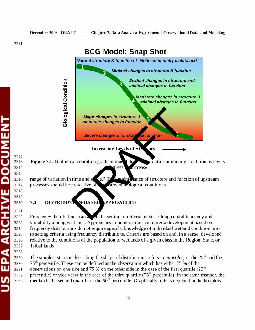
December 2006 - DRAFT Chapter 7. Data Analysis: Experiments, Observational Data, and Modeling
94
3311
Bi o
logi
c al C
ondi
t ion
BCG Model: Snap Shot
Increasing Levels of Stressors
Natural structure & function of biotic community maintained
Minimal changes in structure & function
Evident changes in structure and minimal changes in function
Moderate changes in structure & minimal changes in function
Major changes in structure & moderate changes in function
Severe changes in structure & function
1122
33
44
55
66
3312 Figure 7.1. Biological condition gradient model describing biotic community condition as levels 3313
of stressors increase. 3314 3315 range of variation in time and space.” Thus maintenance of structure and function of upstream 3316 processes should be protective of downstream biological conditions. 3317 3318 3319 7.3 DISTRIBUTION-BASED APPROACHES 3320
3321 Frequency distributions can aid in the setting of criteria by describing central tendency and 3322 variability among wetlands. Approaches to numeric nutrient criteria development based on 3323 frequency distributions do not require specific knowledge of individual wetland condition prior 3324 to setting criteria using frequency distributions. Criteria are based on and, in a sense, developed 3325 relative to the conditions of the population of wetlands of a given class in the Region, State, or 3326 Tribal lands. 3327 3328 The simplest statistic describing the shape of distributions refers to quartiles, or the 25th and the 3329 75th percentile. These can be defined as the observation which has either 25 % of the 3330 observations on one side and 75 % on the other side in the case of the first quartile (25th 3331 percentile) or vice versa in the case of the third quartile (75th percentile). In the same manner, the 3332 median is the second quartile or the 50th percentile. Graphically, this is depicted in the boxplots 3333
DRAFT

December 2006 - DRAFT Chapter 7. Data Analysis: Experiments, Observational Data, and Modeling
95
as the box length, the lower extreme represents the first quartile, the upper extreme represents 3334 the third quartile, the area inside the box encompassing 50 % of the data. 3335 3336 Distributions of nutrient exposure metrics or response variables can be developed to represent 3337 either an entire population of wetlands, or only a subset of these considered to be minimally 3338 impacted. In either case, a population of wetlands should be defined narrowly enough through 3339 classification so that the range in attributes due to natural variability does not equal or exceed the 3340 range in attributes related to anthropogenic effects. The effects of natural variability can be 3341 minimized by classifying wetlands by type and/or region. Nutrient ecoregions define one 3342 potential regional classification system (USEPA 2000). Alternatively, thresholds in landscape or 3343 watershed attributes defining natural breakpoints in nutrient concentrations can be determined 3344 objectively through procedures such as classification and regression tree (CART) analysis 3345 (Robertson et. al., 2001). 3346 3347 3348 7.4 RESPONSE-BASED APPROACHES 3349
3350 Indicators characterized as "response" or "condition" metrics should be distinguished from 3351 "stressor" or "causal" indicators, such as nutrient concentrations (Paulsen et al., 1991; USEPA 3352 1998a; Stevenson 2004a). While both "response" and "causal" indicators could be used in a 3353 single multimetric index, it is recommended that separate multimetric indices be used for 3354 "response" and "causal" assessment. Distinguishing between "response" and "causal" indices can 3355 be accomplished utilizing a risk assessment approach with separate hazard and exposure 3356 assessments that are linked to response-stressor relationships (USEPA 1996; 1998a; Stevenson 3357 1998; Stevenson et al., 2004a, b). A multimetric index that specifically characterizes "responses" 3358 can be used to clarify goals of management (maintenance or restoration of ecological attributes) 3359 and to measure whether goals have been attained with nutrient management strategies. 3360 Response-based multimetric indices can also be used more directly for natural resource damage 3361 assessments than multimetric indices with response and causal variables. 3362 3363 Factors that should be considered in selecting indicators include conceptual relevance (relevance 3364 to the assessment and to ecological function), feasibility of implementation (data collection 3365 logistics, information management, quality assurance, cost), response variability (measurement 3366 error, seasonal variability, interannual variability, spatial variability, discriminatory ability), and 3367 interpretation and utility (data quality objectives, assessment thresholds, link to management 3368 actions) (Jackson et al., 2000). Of these factors, cost, response variability, and ability to meet 3369 data quality objectives can be assessed through quantitative methods. An analytical 3370 understanding of the factors that affect wetlands the most will also help States and Tribes 3371 develop the most effective monitoring and assessment strategies 3372 3373 Designated uses such as contact recreation and drinking water may not be applicable to 3374 wetlands, hence, it may not be readily apparent what the relative significance of changes in 3375
DRAFT

December 2006 - DRAFT Chapter 7. Data Analysis: Experiments, Observational Data, and Modeling
96
different primary producers is for organisms at higher trophic levels. Wetland food webs have 3376 traditionally been considered to be detritus-based (Odum and de la Cruz 1967; Mann 1972, 3377 1988). However, more recent research on wetland food webs utilizing stable isotope analysis 3378 have identified the importance of phytoplankton, periphyton, or benthic algae as the base of the 3379 food chain for higher trophic levels (Fry 1984, Kitting et al., 1984, Sullivan and Moncreiff 1990, 3380 Hamilton et al., 1992, Newell et al., 1995, Keough et al., 1996); in these cases, it would be 3381 particularly important to monitor shifts in algal producers. 3382 3383 Empirical relationships can be derived directly between water quality parameters such as total P 3384 or transparency and wetland biological responses. Unlike lakes or streams, the level of algal 3385 biomass corresponding to aesthetic problems or ecological degradation in wetlands is not readily 3386 defined, so that defining a TP-chlorophyll a relationship based on water column measurements is 3387 not likely to be useful. However, in some wetlands such as coastal Great Lakes, the loss of 3388 submerged aquatic vegetation biomass and/or diversity with increased eutrophication provides 3389 an ecologically significant endpoint (Lougheed et al., 2001). Reductions in submerged plant 3390 species diversity was associated with increases in turbidity, total P, total N, and chlorophyll a, 3391 suggesting that a trophic state index incorporating multiple parameters might be a better 3392 predictor than a single variable such as total P (Carlson 1977). 3393 3394 Models describing empirical relationships can include linear or nonlinear univariate forms with a 3395 single response metric, multivariate with multiple response metrics, a series of linked 3396 relationships, and simulation models. The simplest forms of linear univariate approaches are 3397 correlation and regression analyses; these approaches have the advantage that they are simple to 3398 perform and transparent to the general public. When assessment thresholds can be determined 3399 based on severity of effect or difference from reference conditions, such that associated exposure 3400 criteria can be derived, linear forms should be adequate. In the case of nonlinear relationships, 3401 data can generally be transformed to linearize the relationship. However, if it is desired to 3402 identify the inflection point in a curvilinear relationship as an indicator of rapid ecological 3403 change, alternative data analysis methods are available, including changepoint analysis 3404 (Richardson and Qian 1999) and piecewise iterative regression techniques (Wilkinson 1999). 3405 3406 Multivariate models are useful for relating nutrient exposure metrics to community-level 3407 responses. Both parametric and nonparametric (nonmetric dimensional scaling or NMDS) 3408 ordination procedures can be used to define axes or gradients of variation in community 3409 composition based on relative density, relative abundance, or simple presence-absence measures 3410 (Gauch 1982, Beals 1984, Heikkila 1987, Growns et al., 1992). Ordination scores then can be 3411 regressed against nutrient exposure metrics, as an indicator of a composite response (McCormick 3412 et al., 1996). Direct gradient analysis techniques such as canonical correspondence analysis can 3413 be used to determine which combination of nutrient exposure variables predict a combination of 3414 nutrient response variables as a first step in deriving multimetric exposure and response variables 3415 (Cooper et al., 1999). Indicator analysis can be used to determine which subset of species best 3416 discriminate between reference sites with low nutrient loadings versus potentially impacted sites 3417
DRAFT
December 2006 - DRAFT Chapter 7. Data Analysis: Experiments, Observational Data, and Modeling
97
with high loadings, or weighted averaging techniques can be used to infer nutrient levels from 3418 species composition (McCormick et al., 1996, Cooper et al., 1999, Jensen et al., 1999). In the 3419 latter case, paleoecological records can be examined to infer historic changes in total P levels 3420 from macrophyte pollen or diatom frustrules, which will be particularly valuable in the absence 3421 of sites representing reference condition (Cooper et al., 1999, Jensen et al.,1999). 3422 3423 Some ecohydrological models have been derived that incorporate the effect of multiple stressors 3424 (hydrology, eutrophication, acidity) on wetland vegetation, thus providing a link between 3425 process-based models and community level response (see Olde Venterink and Wassen 1997 for 3426 review). These models are based on 1) a combination of expert opinion to estimate species 3427 sensitivities, supplemented by multivariate classification of vegetation and environmental data to 3428 determine boundaries of species guilds, or 2) field measurements used to derive logistic models 3429 to quantify dose-response. These approaches could be used to derive wetland nutrient criteria for 3430 the US, provided that models could be calibrated using species and response curves developed 3431 using data for the US. Most multiple-stressor models for wetland vegetation have been calibrated 3432 using data from western Europe (Olde Venterink and Wassen 1997). Latour and colleagues 3433 (Latour and Reiling 1993, Latour et al., 1994) have suggested a mechanism for setting nutrient 3434 standards using the occurrence probability of species along a trophic gradient to extrapolate 3435 maximum tolerable concentrations that protect 95% of species. 3436 3437 A series of linked empirical relationships for wetlands may be most effective for developing 3438 nutrient criteria. Linked empirical relationships may be most useful in cases where integrative 3439 exposure measurements such as sediment nutrient concentrations are more sensitive predictors of 3440 shifts in community composition, or algal P limitation, or other ecological responses 3441 (phosphatase enzyme assays; Qian et al., 2003) than are spatially and temporally heterogeneous 3442 water column nutrient concentrations. In these cases, it may be important to develop one set of 3443 relationships between nutrient loading and exposure indicators for a subset of sites at which 3444 intensive monitoring is done, and another set of relationships between nutrient exposure and 3445 ecological response indicators for a larger sample population (Qian et al., 2003). 3446 3447 3448 7.5 PARTITIONING EFFECTS AMONG MULTIPLE STRESSORS 3449
3450 Changes in nutrient concentrations within or loadings to wetlands often co-occur with other 3451 potential stressors such as changes in hydrologic regime and sediment loading. In a few cases, 3452 researchers have been able to separate the simple effects of nutrient addition through 3453 manipulations of mesocosms (Busnardo et al., 1992, Gabor et al. 1994, Murkin et al., 1994, 3454 McDougal et al., 1997, Hann and Goldsborough 1997), segments of natural systems (Richardson 3455 and Qian 1999, Thormann and Bayley 1997), or whole wetlands (Spieles and Mitsch 2000). In 3456 other cases, both simple and interactive effects have been examined experimentally, e.g., to 3457 separate effects of hydrologic regime from nutrient loading (Neill 1990a, b; Neill 1992, Bayley 3458 et al., 1985). If nutrient effects are examined by comparing condition of natural wetlands along a 3459
DRAFT
December 2006 - DRAFT Chapter 7. Data Analysis: Experiments, Observational Data, and Modeling
98
loading or concentration gradient, effects of other driving factors can be minimized by making 3460 comparisons among wetlands of similar hydrogeomorphic type and climatic regime within a 3461 well-defined sampling window. In addition, multivariate techniques for partitioning effects 3462 among multiple factors can be used, such as partial CCA or partial redundancy analysis (Cooper 3463 et al., 1999, Jensen et al., 1999). 3464 3465 3466 7.6 STATISTICAL TECHNIQUES 3467
3468 Quantitative methods can be used to assess metric cost, evaluation, response variability, and 3469 ability to meet data quality objectives. The most appropriate method varies with respect to the 3470 indicator or variable being considered. In general, statistical techniques are aimed at making 3471 conjectures or inferences about a population’s values or relationships between variables in a 3472 sample randomly taken from the population of interest. In these terms, population is defined as 3473 all possible values that a certain parameter may take. For example, in the case of total 3474 phosphorus levels present in marsh sediments in nutrient ecoregion VII, the total population 3475 would be determined if all the marshes in that ecoregion were sampled, which would negate the 3476 need for data analysis. Practically, a sample is taken from the population and the characteristics 3477 associated with that sample (mean, standard deviation) are “transferred” to the entire population. 3478 Many of the basic statistical techniques are designed to quantify the reliability of this transferred 3479 estimate by placing a confidence interval over the sample-derived parameter. More complex 3480 forms of data analysis involve comparisons of these parameters from different populations (for 3481 example, comparison between sites) or the establishment of complex data models that are 3482 thought to better describe the original population structure (for example, regression). They are 3483 still basic inference techniques that utilize sample characteristics to make conjectures about the 3484 original population. 3485 3486 A basic and typical issue facing any type of sampling design is the number of samples that 3487 should be taken to be confident in the translation from samples to population. The degree of 3488 confidence required should be defined as data quality objectives by the end-user and should 3489 identify the expected statistical rigor for those objectives to be met. There are extensive texts on 3490 types and manners of sampling schemes; these will not be discussed here. This section is geared 3491 to determining the minimum data set recommended to work with subsequent sections of the data 3492 analysis chapter. In interpreting the results of various forms of data analysis, an acceptable level 3493 of statistical error is formulated, this is called type I error, or alpha (α). Type I error can be 3494 defined as the probability of rejecting the null hypothesis (H0) when this is actually true. In 3495 setting the type I error rate, the type II error rate is also specified. The type II error rate, or beta 3496 (β), is defined as failing to reject the null hypothesis when it is actually false, i.e., declaring that 3497 no significant effect exists when in reality this is the case. In setting the type I error rate, an 3498 acceptable level of risk is recommended, the risk of concluding that a significance exists when 3499 this is not the case in reality, i.e., the risk of a “false positive”(type I error) or “false negative” 3500 (type II error). The concepts of Type I and Type II errors are introduced in Chapter 4 with 3501
DRAFT

December 2006 - DRAFT Chapter 7. Data Analysis: Experiments, Observational Data, and Modeling
99
reference to sampling design and monitoring, and more fully discussed in Chapter 8 with 3502 reference to criteria development. 3503 3504 In experimental or sampling design, of greater interest is a statistic associated with beta (β) , 3505 specifically 1 – β, which is the power of a statistical tests. Power is the ability of the statistical 3506 test to indicate significance based on the probability that it will reject a false null hypothesis. 3507 Statistical power depends on the level of acceptable statistical significance (usually expressed as 3508 a probability 0.05 – 0.001 (5% -1%) and termed the α level); the level of power dictates the 3509 probability of “success”, or identifying the effect. Statistical power is a function of three factors; 3510 effect size, alpha (α ) and sample size, the relationship between the three factors being relatively 3511 complex. 3512 3513 3514 1. Effect size is defined as the actual magnitude of the effect of interest. This could be the 3515
difference between two means, or the actual correlation between the variables. The 3516 relationship between the effect size and power is intuitive; if the effect size is large (for 3517 example, a large difference between means) this results in a concomitantly large power. 3518
3519 2. Alpha is related to power; to achieve a higher level of significance, power decreases if 3520
other factors are kept constant. 3521 3522 3. Sample size. Generally, this is the easiest factor to control. If the two preceding factors 3523
are set, increased sample sizes will always result in a greater power. 3524 3525 As indicated before, the relationship between these three factors is complex and depends on the 3526 nature of the intended statistical analysis. An online guide for selecting appropriate statistical 3527 procedures is available at: http://www.socialresearchmethods.net/ . Software packages for 3528 performing power analysis have been reviewed by Thomas and Krebs (1997). Online power 3529 calculations have been made available by several statistical faculty, and are available at these 3530 websites: http://www.math.yorku.ca/SCS/, http://calculators.stat.ucla.edu/powercalc/, 3531 http://www.surveysystem.com/sscalc.htm, 3532 http://www.health.ucalgary.ca/~rollin/stats/ssize/index.html, http://www.stat.ohio-3533 state.edu/~jch/ssinput.html, http://www.stat.uiowa.edu. Additional websites are also listed in 3534 Chapter 4 that emphasize designs for monitoring with statistical rigor. 3535 3536 Metric response variability can be evaluated by examining the signal to noise ratio (signal:noise) 3537 along a gradient of nutrient concentrations or loading rates (Reddy et al. 1999). The power of 3538 regression analyses can be determined using the power function for a t-test. Optimization of the 3539 design, such as the spacing, number of levels of observations, and replication at each level, 3540 depend on the purpose of the regression analysis (Neter et al. 1983). 3541 3542 MULTIMETRIC INDICIES 3543 3544
DRAFT

December 2006 - DRAFT Chapter 7. Data Analysis: Experiments, Observational Data, and Modeling
100
Multimetric indices are valuable for summarizing and communicating results of environmental 3545 assessments and is one approach in developing criteria. Furthermore, preservation of the biotic 3546 integrity of algal assemblages, as well as fish and macroinvertebrate assemblages, may be an 3547 objective for establishing nutrient criteria. Multimetric indices for stream macroinvertebrates and 3548 fish are common (e.g., Kerans and Karr 1994, Barbour et al. 1999), and multimetric indices with 3549 benthic algae have recently been developed and tested on a relatively limited basis (Kentucky 3550 Division of Water 1993; Hill et al. 2000). Efforts are underway to develop multi-metric indices 3551 of biotic integrity for wetlands, and methods modules are available for characterizing wetland 3552 algal, plant, macroinvertebrate, amphibian, and bird communities 3553 (http://www.epa.gov/waterscience/criteria/wetlands/ ). Methods for multi-metric indices are 3554 well developed for streams, and these methods are readily transferable to wetlands. However, 3555 higher trophic levels do not often directly respond to nutrients, and therefore may not be as 3556 sensitive to relatively small changes in nutrient concentrations as algal assemblages. It is 3557 recommended that relations between biotic integrity of algal or vegetation assemblages and 3558 nutrients be defined and then related to biotic integrity of macroinvertebrate and fish 3559 assemblages in a stepwise, mechanistic fashion. The practitioner should realize however, that 3560 wetlands with a history of high nutrient loadings have often lost the most sensitive species and in 3561 these cases higher trophic level species may prove to be the best indicators of current nutrient 3562 loadings and wetland nutrient condition. 3563 3564 This section provides an overview for developing a multimetric index that will indicate shifts in 3565 primary producers that are associated with trophic status in wetlands. The first step in developing 3566 a multimetric index of trophic status is to select a set of ecological attributes that respond to 3567 human changes in nutrient concentrations or loading. Attributes that respond to an increase in 3568 human disturbance are referred to as metrics. Six to ten metrics should be selected for the index 3569 based on their sensitivity to human activities that increase nutrient availability (loading and 3570 concentrations), their precision, and their transferability among regions and habitat types. 3571 Selected metrics also should respond to the breadth of biological responses to nutrient conditions 3572 (see discussion of metric properties in McCormick and Cairns 1994). 3573 3574 Effects of nutrients on primary producers and effects of primary producers on the biotic integrity 3575 of macroinvertebrates and fish should be characterized to aid in developing nutrient criteria that 3576 will protect designated uses related to aquatic life (e.g., Miltner and Rankin 1998, King and 3577 Richardson 2002). 3578 3579 Another approach for characterizing biotic integrity of assemblages as a function of trophic 3580 status is to calculate the deviation in species composition or growth forms at assessed sites from 3581 composition in the reference condition. Similarity or dissimilarity indices can be used for the 3582 determining the differences in biotic integrity of a wetland in comparison to the reference 3583 condition. Multivariate similarity or dissimilarity indices need to be calculated for multivariate 3584 attributes such as taxonomic composition (Stevenson 1984; Raschke 1993) as defined by relative 3585
DRAFT
December 2006 - DRAFT Chapter 7. Data Analysis: Experiments, Observational Data, and Modeling
101
abundance of different growth forms or species, or species presence/absence. One standard form 3586 of these indices is percent community similarity (PSc, Whittaker 1952): 3587 3588
PSc =Σi=1,s min(ai,bi) 3589 3590
Here ai is the percentage of the ith species in sample a, and bi is the percentage of the same ith 3591 species in a subsequent sample, sample b. 3592 3593 A second common community similarity measurement is based on a distance measurement 3594 (which is actually a dissimilarity measurement, rather than similarity measurement, because the 3595 index increases with greater dissimilarity, Stevenson 1984; Pielou 1984). Euclidean distance 3596 (ED) is a standard distance dissimilarity index, where: 3597 3598
ED = √( Σi=1(ai-bi)2) 3599 3600
Log-transformation of species relative abundances in these calculations can increase precision of 3601 metrics by reducing variability in the most abundant taxa. However, the practitioner should also 3602 be aware that transformation, while reducing variability, often decreases sensitivity and the 3603 ability to distinguish true fine scale changes in community and species composition. 3604 Theoretically and empirically, we expect to find that multivariate attributes based on taxonomic 3605 composition more precisely and sensitively respond to nutrient conditions than do univariate 3606 attributes, for instance multimetric algal assemblages (see discussions in Stevenson and Pan 3607 (1999)). 3608 3609 To develop the multimetric index, metrics should be selected and their values normalized to a 3610 standard range such that they all increase with trophic status. Criteria for selecting metrics can be 3611 found in McCormick and Cairns (1994) or many other references. Basically, sensitive and 3612 precise metrics should be selected for the multimetric index and selected metrics should 3613 represent a broad range of impacts and perhaps, designated uses. Values can be normalized to a 3614 standard range using many techniques. For example, if 10 metrics are used and the maximum 3615 value of the multimetric index is defined as 100, all ten metrics should be normalized to the 3616 range of 10 so that the sum of all metrics would range between 0 and 100. The multimetric index 3617 is calculated as the sum of all metrics measured in a system. A high value of this multimetric 3618 index of trophic status would indicate high impacts of nutrients and should be a robust (certain 3619 and transferable) and moderately sensitive indicator of nutrient impacts in a stream. A 1-3-5 3620 scaling technique is commonly used with aquatic invertebrates (Barbour et al. 1999; Karr and 3621 Chu 1999) and could be used with a multimetric index of trophic status as well. 3622 3623 3624 7.7 LINKING NUTRIENT AVAILABILITY TO PRIMARY PRODUCER RESPONSE 3625
3626
DRAFT
December 2006 - DRAFT Chapter 7. Data Analysis: Experiments, Observational Data, and Modeling
102
When evaluating the relationships between nutrients and primary producer response within 3627 wetland systems, it is important to first understand which nutrient is limiting. Once the limiting 3628 nutrient is defined, critical nutrient concentrations can be specified and nutrient-response 3629 relationships developed. 3630 3631 DEFINING THE LIMITING NUTRIENT 3632 3633 The first step in identifying nutrient-producer relationships should be to define the limiting 3634 nutrient. Limiting nutrients will control biomass and productivity within a system. However, 3635 non-limiting nutrients may have other impacts, e.g., toxicological effects related to ammonia 3636 concentrations in sediments or effects on competitive interactions which determine vegetation 3637 community composition (Guesewell et al. 2003). A review of fertilization studies indicated that 3638 vegetation N:P mass ratios are a good predictor of the nature of nutrient limitation in wetlands, 3639 with N:P ratios > 16 indicating P limitation at a community level, and N:P ratios < 14 indicative 3640 of N limitation (Koerselman and Meuleman 1996). Guesewell et al. (2003) found that vegetation 3641 N:P ratios were a good predictor of community-level biomass response to fertilization by N or P, 3642 but for individual species, were only predictive of P-limitation and could not distinguish between 3643 N-limitation, co-limitation, or no limitation. Likewise, N, P, and K levels in wet meadow and fen 3644 vegetation were found to be correlated with estimated supply rates or extractable fractions in 3645 soils (Odle Venterink et al. 2002). A survey of literature values of vegetation and soil total N:P 3646 ratios by Bedford et al. (1999) indicated that many temperate North American wetlands are 3647 either P-limited or co-limited by N and P, especially those with organic soils. Only marshes have 3648 N:P ratios in both soils and plants indicative of N limitation, while soils data suggest that most 3649 swamps are also N-limited. 3650 3651 Many experimental procedures are used to determine which nutrient (N, P, or carbon) limits 3652 algal growth. Algal growth potential (AGP) bioassays are very useful for determining the 3653 limiting nutrient (USEPA 1971). Yet, results from such assays usually agree with what would 3654 have been predicted from N:P biomass ratios, and in some cases N:P ratios in the water. Limiting 3655 nutrient-potential biomass relationships from AGP bottle tests are useful in projecting maximum 3656 potential biomass in standing or slow-moving water bodies. However, they are not as useful in 3657 fast-flowing, and/or gravel or cobble bed environments. Also, the AGP bioassay utilizes a single 3658 species which may not be representative of the response of the natural species assemblage. 3659 3660 Limitation may be detected by other means, such as alkaline-phosphatase activity, to determine 3661 if phosphorus is limiting. Alkaline phosphatase is an extracellular enzyme excreted by some 3662 algal species and from roots in some macrophytes in response to P limitation. This enzyme 3663 hydrolyzes phosphate ester bonds, releasing orthophosphate (PO4) from organic phosphorus 3664 compounds (Mullholland et al. 1991). Therefore, the concentration of alkaline phosphatase in the 3665 water can be used to assess the degree of P limitation. Alkaline phosphatase activity, monitored 3666 over time in a waterbody, can be used to assess the influence of P loads on the growth limitation 3667 of algae (Richardson and Qian 1999). 3668
DRAFT
December 2006 - DRAFT Chapter 7. Data Analysis: Experiments, Observational Data, and Modeling
103
3669 There have been no empirical relationships published relating nutrient concentrations or inputs 3670 to wetland chlorophyll a or productivity levels as there have been for streams and lakes. This is 3671 likely due to the large number of factors interacting with nutrients that determine net ecological 3672 effects in wetlands. For example, eutrophication of Great Lakes coastal wetlands and increases 3673 in agricultural area in upstream watersheds have been correlated with decreases in diversity of 3674 submerged aquatic vegetation, yet researchers were unable to uncouple the effects of nutrients 3675 from those of turbidity (Lougheed et al. 2001). Even in experimentally controlled settings, where 3676 it is possible to separate increased suspended solids loadings from nutrient loadings, effects of 3677 nutrients depend heavily on other factors such as periodicity of nutrient additions (pulse vs. press 3678 loadings; Gabor et al. 1994, Murkin et al., 1994, Hann and Goldsborough 1997, McDougal et al. 3679 1997), water regime (Neill 1990a, b; Thormann and Bayley 1997), food web structure 3680 (Goldsborough and Robinson 1996) and time lags (Neill 1990a, b). It is important in 3681 experimental settings to utilize adequate controls for water additions that may accompany 3682 nutrients (Bayley et al. 1985); in empirical comparisons from field data, it may be difficult if not 3683 impossible to separate out these effects. Day et al. (1988) propose a general conceptual model 3684 describing responses of different wetland plant guilds in riverine wetlands based on a 3685 combination of disturbance regime, hydrologic regime, and nutrients. In the latter case, proper 3686 classification of sites based on disturbance and hydrologic regime prior to describing reference 3687 condition, help to adequately separate out nutrient-related effects and to explain differences in 3688 response. 3689 3690 The significance of food web structure in determining nutrient effects does not preclude deriving 3691 predictive nutrient-primary producer relationships, or minimize the importance of describing 3692 significant impacts. However, it does highlight the importance of adequately characterizing the 3693 trophic structure of wetlands prior to comparison, especially the number of trophic levels (e.g., 3694 presence or absence of planktivorous fish) and examining interactive effects on multiple classes 3695 of primary producers: phytoplankton, epipelon, epiphytic algae, metaphyton, and macrophytes 3696 (Goldsborough and Robinson 1996, McDougal et al., 1997). In some cases, addition of nutrients 3697 may have little or no effect on some components such as benthic algae, but can create significant 3698 shifts in primary productivity among others, such as a loss of macrophytes and associated 3699 epiphytes with an increase in inedible filamentous metaphyton and shading of the water column 3700 (McDougal et al., 1997). 3701
DRAFT

December 2006 DRAFT Chapter 8. Criteria Development
104
Chapter 8 Criteria Development 3702 3703 3704 8.1 INTRODUCTION 3705
3706 This chapter describes recommendations for setting scientifically defensible criteria for nutrients 3707 in wetlands by using data that address causal and biotic response variables. Causal variables 3708 (external nutrient loading, soil extractable P, soil extractable N, total soil N and P, and water 3709 column N and P), and biotic response variables (vegetation N and P, biomass, species 3710 composition, and algal N and P) and the supporting variables (hydrologic condition, 3711 conductivity, soil pH, soil bulk density, particle size distribution, and soil organic matter), as 3712 described in Chapter 5, provide an overview of environmental conditions and nutrient status of 3713 the wetland; these parameters are considered critical to nutrient assessment in wetlands. (See 3714 also Chapter 5). Several recommended approaches that water quality managers can use to derive 3715 numeric criteria in combination with other biological response variables are presented. These 3716 recommended approaches can be used alone, in combination, or may be modified for use by 3717 State/Tribal water quality managers to derive criteria for wetland systems in their State/Tribal 3718 waters. Recommended approaches for numeric nutrient criteria development presented here 3719 include: 3720 3721
• the use of reference conditions to characterize natural or minimally impaired wetland 3722 systems with respect to causal and exposure indicator variables, 3723
• applying predictive relationships to select nutrient concentrations that will protect 3724 wetland structure and/or function, and 3725
• developing criteria from established nutrient exposure-response relationships (as in the 3726 peer-reviewed published literature). 3727
3728 The first approach is based on the assumption that maintaining nutrient levels within the range of 3729 values measured for reference systems will maintain the biological integrity of wetlands. This 3730 presumes that a sufficient number of reference systems can be identified. The second two 3731 approaches are response-based, hence the level of nutrients associated with biological 3732 impairment should be used to identify criteria. Ideally, both kinds of information (background 3733 variability and exposure-response relationships) will be available for criteria development. 3734 Recommendations are also presented for deriving criteria based on the potential for effects to 3735 downstream receiving waters (i.e., the lake, reservoir, stream, or estuary influenced by 3736 wetlands). The chapter concludes with a recommended process for evaluating proposed criteria, 3737 suggestions of how to interpret and apply criteria, considerations for sampling for comparison to 3738 criteria, potential modifications to established criteria, and final implementation of criteria into 3739 water quality standards. 3740 3741
DRAFT
December 2006 DRAFT Chapter 8. Criteria Development
105
The RTAG is composed of State, Tribal, and Regional specialists that will help the Agency and 3742 States/Tribes establish nutrient criteria for adoption into their water quality standards. Expert 3743 evaluations are important throughout the criteria development process. The data upon which 3744 criteria are based and the analyses performed to arrive at criteria should be assessed for veracity 3745 and applicability. 3746 3747 8.2 METHODS FOR DEVELOPING NUTRIENT CRITERIA 3748
3749 The following discussions focus on three general methods that can be used in developing 3750 nutrient criteria. First, identification of reference or control systems for each established wetland 3751 type and class should be based on either best professional judgment (BPJ) or percentile 3752 selections of data plotted as frequency distributions. The second method uses refinement of 3753 classification systems, models, and/or examination of system biological attributes to assess the 3754 relationships among nutrients, vegetation or algae, soil, and other variables. Finally, the third 3755 method identifies published nutrient and vegetation, algal, and soil relationships and values that 3756 may be used (or modified for use) as criteria. A weight of evidence approach with multiple 3757 attributes that combines one or more of these three approaches should produce criteria of 3758 greater scientific validity. 3759 3760 USING REFERENCE CONDITION TO ESTABLISH CRITERIA 3761 3762 One approach to consider in setting criteria is the concept of reference condition. This approach 3763 involves using relatively undisturbed wetlands as reference systems to serve as examples for the 3764 natural or least disturbed ecological conditions of a region. Three recommended ways of using 3765 reference condition to establish criteria are: 3766 3767 1. Characterize reference systems for each class within a region using best professional 3768
judgment and use these reference conditions to define criteria. 3769 3770 2. Identify the 75th to 95th percentile of the frequency distribution for a class of reference 3771
wetlands as defined in Chapter 3 and use this percentile to define the criteria. 3772 3773 3. Calculate a 5th to 25th percentile of the frequency distribution of the general population of 3774
a class of wetlands and use the selected percentile to define the criteria. 3775 3776 Defining the nutrient condition of wetlands within classes will allow the manager to identify 3777 protective criteria and determine which systems may benefit from management action. Criteria 3778 that are identified using reference condition approaches may require comparisons to similar 3779 systems in other States or Tribes that share the ecoregion so that criteria can be validated. The 3780 comparison process should also be developed and documented. 3781 3782
DRAFT

December 2006 DRAFT Chapter 8. Criteria Development
106
Reference wetlands should be identified for each class of wetland within a state or tribal 3783 ecoregion and then characterized with respect to external nutrient loading, water column N and 3784 P, biotic response variables (macrophytes, algae, soils) and supporting environmental conditions. 3785 Wetlands classified as reference quality should be verified by comparing the data from the 3786 reference systems to general population data for each wetland class. Reference systems should 3787 be minimally disturbed and should have biotic response values that reflect this condition. 3788 3789 Conditions at reference sites may be characterized using either of two frequency distribution 3790 approaches ( see 2 and 3 above). In both approaches, an optimal reference condition value is 3791 selected from the distribution of an available set of wetland data for a given wetland class. This 3792 approach may be of limited value at this time, because few States or Tribes currently collect 3793 wetland monitoring data. However, as more wetlands are monitored and more data become 3794 available, this approach may become more viable. 3795 3796 In the first frequency distribution approach, a percentile (75th – 95th is recommended) is selected 3797 from the distribution of causal and biotic response variables of reference systems selected a 3798 priori based on very specific criteria (i.e., highest quality or least impacted wetlands for that 3799 wetland class within a region). The values for variables at the selected quartile are used as the 3800 basis for nutrient criteria. 3801 3802 If reference wetlands of a given class are rare within a given region, or if inadequate information 3803 is available to assign wetlands with historic nutrient data as “reference” versus “impacted” 3804 wetlands, another approach may be necessary. The second frequency distribution approach 3805 involves selecting a percentile of (1) all wetland data in the class (reference and non-reference) 3806 or (2) a random sample distribution of all wetland data within a particular class. Due to the 3807 random selection process, a lower percentile should be selected because the sample distribution 3808 is expected to contain some degraded systems. This option is most useful in regions where the 3809 number of legitimate “natural” reference wetlands is usually very small, such as in highly 3810 developed land use areas (e.g., the agricultural lands of the Midwest and the urbanized east or 3811 west coasts). EPA’s recommendation in this case is the 5th to 25th percentile depending upon the 3812 number of “natural” reference systems available. If almost all systems are impaired to some 3813 extent, then a lower percentile, generally the 5th percentile is recommended for selection of 3814 reference wetlands. 3815 3816 Both the 75th percentile for the subset of reference systems and the 5th to 25th percentile from a 3817 representative random sample distribution are only recommendations. The actual distribution of 3818 the observations should be the major determinant of the threshold point chosen. For example, a 3819 bi-modal distribution of sediment or water-column nutrients might indicate a natural breakpoint 3820 between reference and enriched systems. To illustrate, Figure 8.1 shows both options and 3821 illustrates the presumption that these two alternative methods should approach a common 3822 reference condition along a continuum of data points. In this illustration, the 75th percentile of 3823
DRAFT
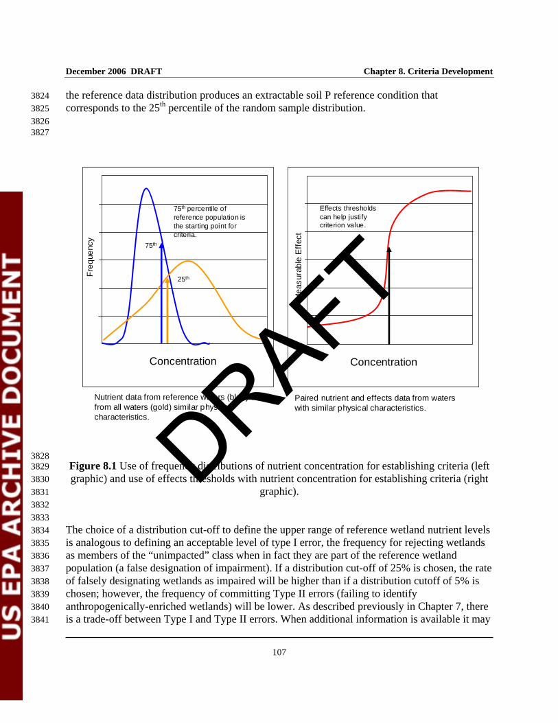
December 2006 DRAFT Chapter 8. Criteria Development
107
the reference data distribution produces an extractable soil P reference condition that 3824 corresponds to the 25th percentile of the random sample distribution. 3825 3826 3827
75th
25th
Freq
uenc
y
Concentration
75th percentile of reference population is the starting point for criteria.
Nutrient data from reference waters (blue) or from all waters (gold) similar physical characteristics.
Mea
sura
ble
Effe
ct
Concentration
Effects thresholds can help justi fy criterion value.
Paired nutrient and effects data from waters with similar physical characteristics.
75th
25th
3828 Figure 8.1 Use of frequency distributions of nutrient concentration for establishing criteria (left 3829 graphic) and use of effects thresholds with nutrient concentration for establishing criteria (right 3830
graphic). 3831 3832 3833 The choice of a distribution cut-off to define the upper range of reference wetland nutrient levels 3834 is analogous to defining an acceptable level of type I error, the frequency for rejecting wetlands 3835 as members of the “unimpacted” class when in fact they are part of the reference wetland 3836 population (a false designation of impairment). If a distribution cut-off of 25% is chosen, the rate 3837 of falsely designating wetlands as impaired will be higher than if a distribution cutoff of 5% is 3838 chosen; however, the frequency of committing Type II errors (failing to identify 3839 anthropogenically-enriched wetlands) will be lower. As described previously in Chapter 7, there 3840 is a trade-off between Type I and Type II errors. When additional information is available it may 3841
DRAFT

December 2006 DRAFT Chapter 8. Criteria Development
108
be possible to justify a range of values that are representative of least-impaired wetlands that 3842 would reduce Type I errors on a system by system basis. 3843 3844 It is important to understand that any line drawn through the data may have certain ramifications; 3845 wetlands in poor condition (on the right) should be dealt with through restoration. The wetlands 3846 to the left of the line have nutrient conditions that are protective of aquatic life and should be 3847 managed to maintain their nutrient condition, i.e. their nutrient concentrations should remain 3848 stable to be protective of aquatic life. These wetlands should be protected according to the 3849 State’s or Tribe’s approved antidegradation policy, and through continued monitoring to assure 3850 that future degradation is prevented. 3851 3852 State or Tribal water quality managers also may consider analyzing wetlands data based on 3853 designated use classifications. Using this approach, frequency distributions for specific 3854 designated uses could be examined and criteria proposed based on maintenance of high quality 3855 systems that are representative of each designated use. For example one criterion could be 3856 derived that protects superior quality wetland habitat (SWLH) and a second criterion could be 3857 identified that maintains good quality wetland habitat (function maintained but some loss of 3858 sensitive species (Figure 8.2); see Office of Water tiered aquatic life use training module: 3859 (http://www.epa.gov/waterscience/biocriteria/modules/wet101-05-alus-monitoring.pdf). This 3860 recommended approach is designated as the Tiered Aquatic Life Use (TALU), and is being 3861 developed by the EPA Office of Water in a more detailed publication. Using this approach, a 3862 criterion range is created and a greater number of wetland systems will likely be considered 3863 protective of the designated use. In this case, emphasis may be shifted from managing wetland 3864 systems based on a central tendency to managing towards more pristine systems associated with 3865 Tiers I and II. This approach also will aid in prioritizing systems for protection and restoration. 3866 Subsequent management efforts using this approach should focus on improving wetland 3867 conditions so that, over time, plots of wetland data shift to the left (i.e., improved nutrient 3868 condition) of their initial position. 3869 3870 In summary, frequency distributions can aid in setting criteria by describing the natural potential 3871 and best attainable conditions (reference conditions). The number of divisions or tiers used has 3872 significant implications with respect to system management. A single criterion may limit the 3873 flexibility to make management decisions about whether wetlands are meeting the applicable 3874 water quality standards, and there may be considerable ramifications resulting from that 3875 decision. If the distribution is divided into three tiers, the majority of wetlands may be protective 3876 of their designated use (assuming that these wetlands do not contribute to downstream 3877 degradation of water quality), which will minimize management requirements. The method that 3878 is used may depend on the goals of the individual State or Tribe. Some may wish to set criteria 3879 that encourage all State/Tribal wetland systems to be preserved or restored to reference 3880 conditions. Other managers may consider additional options, such as developing criteria 3881 specifically to protect the designated uses established for wetlands in their region. 3882 3883
DRAFT
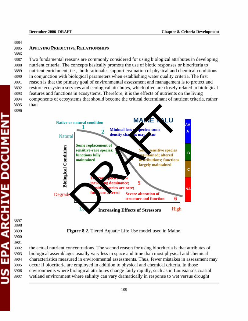
December 2006 DRAFT Chapter 8. Criteria Development
109
3884 APPLYING PREDICTIVE RELATIONSHIPS 3885 3886 Two fundamental reasons are commonly considered for using biological attributes in developing 3887 nutrient criteria. The concepts basically promote the use of biotic responses or biocriteria to 3888 nutrient enrichment, i.e., both rationales support evaluation of physical and chemical conditions 3889 in conjunction with biological parameters when establishing water quality criteria. The first 3890 reason is that the primary goal of environmental assessment and management is to protect and 3891 restore ecosystem services and ecological attributes, which often are closely related to biological 3892 features and functions in ecosystems. Therefore, it is the effects of nutrients on the living 3893 components of ecosystems that should become the critical determinant of nutrient criteria, rather 3894 than 3895 3896
Bio
logi
cal C
ondi
tion
Increasing Effects of StressorsLow High
1Native or natural condition
2 Minimal loss of species; some density changes may occur
3Some replacement of sensitive-rare species; functions fully maintained 4
Some sensitive species maintained; altered distributions; functions largely maintained
5
6
Tolerant species show increasing dominance; sensitive species are rare; functions altered Severe alteration of
structure and function
Natural
DegradedNA
B
C
AA
A
MAINE TALU
3897 3898
Figure 8.2. Tiered Aquatic Life Use model used in Maine. 3899 3900 3901 the actual nutrient concentrations. The second reason for using biocriteria is that attributes of 3902 biological assemblages usually vary less in space and time than most physical and chemical 3903 characteristics measured in environmental assessments. Thus, fewer mistakes in assessment may 3904 occur if biocriteria are employed in addition to physical and chemical criteria. In those 3905 environments where biological attributes change fairly rapidly, such as in Louisiana’s coastal 3906 wetland environment where salinity can vary dramatically in response to wet versus drought 3907
DRAFT

December 2006 DRAFT Chapter 8. Criteria Development
110
years, other techniques will need to be developed. Information on some other techniques can be 3908 found at: Louisiana State University’s School of the Coast and Environment 3909 [http://www.wetlandbiogeochemistry.lsu.edu/ ] and also in interagency efforts through the LA 3910 Dept. of Natural Resources) to assess coastal area ecology. 3911 [http://data.lca.gov/Ivan6/app/app_c_ch9.pdf ] 3912 3913 Multimetric indices are a special form of indicators of biological condition in which several 3914 metrics are used to summarize and communicate in a single number the state of a complex 3915 ecological system. Multimetric indices for macroinvertebrates and fish are used successfully to 3916 establish biocriteria for aquatic systems in many States, and several States are developing 3917 multimetric indices for wetlands (see http://www.epa.gov/owow website). 3918 3919 Another recommended approach is to identify threshold or non-linear biotic responses to nutrient 3920 enrichment. Some biological attributes respond linearly with increasing nutrient concentrations 3921 whereas some attributes change in a non-linear manner. Non-linear changes in metrics indicate 3922 thresholds along environmental gradients where small changes in environmental conditions 3923 cause relatively great changes in a biological attribute. In an example from the Everglades, a 3924 specific level of P concentration and loadings was associated with a dramatic shift in algal 3925 composition and loss of the calcareous algal mats typical of this system (Figure 8.3). Overall, 3926 metrics or indices that change linearly (typically higher-level community attributes such as 3927 diversity or a multimetric index) provide better variables for establishing biocriteria because they 3928 respond to environmental change along the entire gradient of human disturbance. However, 3929 metrics that change in a non-linear manner along environmental gradients are valuable for 3930 determining where along the environmental gradient the physical and chemical criteria should be 3931 set and, correspondingly, how to interpret other biotic response variables of interest (Stevenson 3932 et al. 2004a). 3933 3934 USING DATA PUBLISHED IN THE LITERATURE 3935
3936
Values from the published literature may be used to develop nutrient criteria if a strong rationale 3937 is presented that demonstrates the suitability of these data to the wetland of interest (i.e., the 3938 system of interest should share the same characteristics with the systems used to derive the 3939 published values). Published data, if there is enough of it, could be used to develop criteria for 3940 (1) reference condition, (2) predictive (cause and effect) relationships between nutrients and 3941 biotic response variables, (3) tiered criteria or (4) criteria that exhibit a threshold response to 3942 nutrients. However, published data from similar wetlands should not substitute for collection and 3943 analysis of data from the wetland or wetlands of interest. 3944 3945
DRAFT
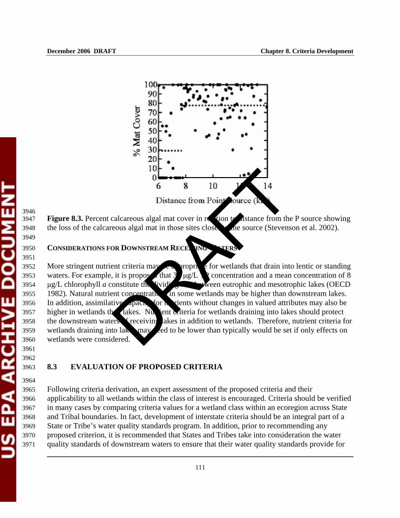
December 2006 DRAFT Chapter 8. Criteria Development
111
3946 Figure 8.3. Percent calcareous algal mat cover in relation to distance from the P source showing 3947 the loss of the calcareous algal mat in those sites closer to the source (Stevenson et al. 2002). 3948 3949
CONSIDERATIONS FOR DOWNSTREAM RECEIVING WATERS 3950 3951 More stringent nutrient criteria may be appropriate for wetlands that drain into lentic or standing 3952 waters. For example, it is proposed that 35 μg/L TP concentration and a mean concentration of 8 3953 μg/L chlorophyll a constitute the dividing line between eutrophic and mesotrophic lakes (OECD 3954 1982). Natural nutrient concentrations in some wetlands may be higher than downstream lakes. 3955 In addition, assimilative capacity for nutrients without changes in valued attributes may also be 3956 higher in wetlands than lakes. Nutrient criteria for wetlands draining into lakes should protect 3957 the downstream waters of receiving lakes in addition to wetlands. Therefore, nutrient criteria for 3958 wetlands draining into lakes may need to be lower than typically would be set if only effects on 3959 wetlands were considered. 3960 3961 3962 8.3 EVALUATION OF PROPOSED CRITERIA 3963
3964 Following criteria derivation, an expert assessment of the proposed criteria and their 3965 applicability to all wetlands within the class of interest is encouraged. Criteria should be verified 3966 in many cases by comparing criteria values for a wetland class within an ecoregion across State 3967 and Tribal boundaries. In fact, development of interstate criteria should be an integral part of a 3968 State or Tribe’s water quality standards program. In addition, prior to recommending any 3969 proposed criterion, it is recommended that States and Tribes take into consideration the water 3970 quality standards of downstream waters to ensure that their water quality standards provide for 3971
DRAFT
December 2006 DRAFT Chapter 8. Criteria Development
112
attainment and maintenance of the water quality standards of downstream waters. (see 40 C.F.R. 3972 131.10(b)). Load estimating models, such as those recommended by EPA (USEPA 1999), can 3973 assist in this determination (see External Nutrient Loading in Chapter 5.3). Water quality 3974 managers responsible for downstream receiving waters also should be consulted. 3975 3976 3977 8.4 INTERPRETING AND APPLYING CRITERIA 3978
3979 After evaluating criteria proposed for each wetland class, determining wetland condition in 3980 comparison with nutrient criteria can be made by following these steps: 3981 3982 1. Calculate duration and frequency of criteria exceedences as well as associated 3983
consequences. This can be done using modeling techniques or correlational analysis of 3984 existing data. 3985
3986 2. Develop and test hypotheses to determine agreement with criteria. Analyze for alpha 3987
(Type I) and beta (Type II) errors (see Chapter 7). 3988 3989 3. Reaffirm appropriateness of criteria for protecting designated uses and meeting water 3990
quality standards (i.e., by effective sampling and monitoring of the wetlands). 3991 3992 The goal is to identify highly protective criteria and standards. Criteria should be based on 3993 ecologically significant changes as well as statistically significant differences in compiled data. 3994 Although criteria are developed exclusively based on scientifically defensible methods, adoption 3995 of water quality standards also allows consideration of social, political, and economic factors. 3996 Thus, it is imperative that some determination is given during the criteria development process to 3997 how criteria can be implemented into standards that are defensible to the public and regulated 3998 communities, and effectively translated into permits, TMDLs, or watershed implementation 3999 plans for nonpoint source nutrient management. 4000 4001 4002 8.5 SAMPLING FOR COMPARISON TO CRITERIA 4003
4004 Sampling to evaluate agreement with the standards implemented from nutrient criteria should be 4005 carefully defined to ensure that state or tribal sampling is compatible with the procedures used to 4006 establish the criteria. If State or Tribal observations are averaged over the year, balanced 4007 sampling is essential and the average should not exceed the criterion. In addition, no more than 4008 ten percent of the observations contributing to that average value should exceed the criterion. 4009 4010
DRAFT

December 2006 DRAFT Chapter 8. Criteria Development
113
It is important to note that, in some regions where nutrient impacts occur seasonally depending 4011 on precipitation and temperature regimes, sampling and assessment should focus on the period 4012 (e.g.,index period) when impacts are most likely to occur. 4013 4014 A load estimating model may be applied to a watershed to back-calculate the criteria 4015 concentration for an individual wetland from its load allocation. This approach to criteria 4016 determination also may be applied on a seasonal basis and should help States/Tribes relate their 4017 wetland criteria with their stream, lake, or estuarine criteria. It also may be particularly important 4018 for criteria developed for wetlands that cross State/Tribal boundaries. 4019 4020 4021 8.6 CRITERIA MODIFICATIONS 4022
4023 There may be specific cases identified by States or Tribes that require modification of 4024 established criteria, either due to unique wetland system characteristics or specific designated 4025 uses approved for a wetland. Two examples of acceptable criteria modifications are presented 4026 below. 4027 4028 SITE SPECIFIC CRITERIA 4029 4030 If a State or Tribe has additional information and data that indicate a different value or set of 4031 values is more appropriate for specific wetland systems than ecoregionally-derived criteria, the 4032 State or Tribe may decide to develop site-specific criteria modifications. This value can be 4033 incorporated into State or Tribal water quality standards and submitted to EPA for approval. 4034 4035 DESIGNATED USE APPROACHES 4036 4037 Once a regional criterion has been established, it should be reviewed and calibrated periodically. 4038 Any State or Tribe in the region with similar classes of wetlands may elect to use the criterion as 4039 the basis for developing its own criteria to protect its designated uses for specific wetland 4040 classes. This is entirely appropriate as EPA expects criteria developed using one of the 4041 approaches recommended here will be protective of aquatic life in wetlands and scientifically 4042 defensible. 4043
DRAFT

December 2006- DRAFT REFERENCES
114
4044 REFERENCES 4045
4046 4047 Adamus P. R. 1992. Choices in Monitoring Wetlands. In: Ecological Indicators. DH McKenzie, 4048
DE Hyatt, VJ McDonald (eds).New York: Elsevier Applied Science, pp. 571-592. 4049 4050 Allen S. E, H. M. Grimshaw, and A. P. Rowland. 1986. Chemical analysis. In: Methods in Plant 4051
Ecology. Moore P. D., S. B. Chapman (eds.).Boston: Blackwell Scientific Publications, 4052 pp. 285-344. 4053
4054 Amoozegar, A. and A. W. Warrick. 1986. Hydraulic conductivity of saturated soils: field 4055
methods. pp. 735-770. In: Methods of Soil Analysis, Part 1, Physical and Mineralogical 4056 Methods. Agronomy monograph No. 9. A. Klute (ed.) American Society of 4057 Agronomy-Soil Science Society of America, Madison WI. 4058
4059 Anderson, J. M. 1976. An ignition method for determination of total phosphorus in lake 4060
sediments. Water Research. 10:329-331. 4061 4062 Angeler, D. G., P. Chow-Fraser, M. A. Hanson, S. Sanchez-Carrille, and K. D. Zimmer. 2003. 4063
Biomanipulation: a useful tool for freshwater wetland mitigation? Freshwater Biology 4064 48:2203-2213. 4065
4066 Apfelbeck, R. S. 1999. Development of biocriteria for wetlands in Montana. Montana Dept. of 4067
Environmental Quality, Helena, MT. 4068 4069 APHA. 1999. Standard Methods for Examination of Water and Wastewater. 21st ed. Eaton, A. 4070
D., L. C. Clesceri, and A. E. Greenberg (eds.). American Public Health Association, 4071 Washington, DC. 4072
4073 Arnold, J. G., J. R. Williams, R. Srinivasan, K. W. King, and R. H. Griggs. 1995. SWAT - Soil 4074
and Water Assessment Tool: Draft Users Manual. USDA-ARS, Temple, TX. 4075 4076 Bailey, R. G. 1976. Ecoregions of the United States (map). Ogden, UT: U.S. Department of 4077
Agriculture, Forest Service. Intermountain Region. Scale 1:7,500,000. 4078 4079 Bailey, S. E; J. Jr. Zoltek, A. J. Hermann, T. J. Dolan, and L. Tortora. 1985. Experimental 4080
manipulation of nutrients and water in a freshwater marsh: Effects on biomass, 4081 decomposition, and nutrient accumulation. Limnology and Oceanography 30: 500-512. 4082
4083 Ball, J. E., M. J. White, G. de R. Innes, and L. Chen. 1993. Application of HSPF on the Upper 4084
Nepean Catchment. In: pp. 343-348. Proceedings of Hydrology and Water Resources 4085 Symposium. Newcastle, New South Wales, Australia. 4086
DRAFT
December 2006- DRAFT REFERENCES
115
4087 Balla, S. A. and J. A. Davis. 1995. Seasonal variation in the macroinvertebrate fauna of wetlands 4088
of differing water regime and nutrient status on the Swan coastal plain, Western 4089 Australia. Hydrobiologia 299:147-161. 4090
4091 Barbour, M. T., J. Gerritsen, B. D. Snyder, and J. B. Stribling. 1999. Rapid Bioassessment 4092
Protocols for Use in Wadeable Streams and Rivers: Periphyton, Benthic 4093 Macroinvertebrates, and Fish 2nd ed. U.S. Environmental Protection Agency, Office of 4094 Water, Washington, DC. EPA 841-B-99-002. 4095
4096 Barko, J. W. 1983. The growth of Myriophyllum spicatum in relation to selected characteristics 4097
of sediment and solution. Aquatic Botany 15:91-103. 4098 4099 Barko, J. W. and R. M. Smart. 1986. Sediment-related Mechanisms of Growth Limitation in 4100
Submersed Macrophytes. J. Ecol. 67(5):1340. 4101 4102 Bayley, S. E. 1985. Effect of Natural Hydroperiod Fluctuations on Freshwater Wetlands 4103
Receiving Added Nutrients. In: Ecological Considerations in Wetlands Treatment of 4104 Municipal Wastewaters. Van Nostrand Reinhold Company New York. pp. 180-9 4105
4106 Bayley, S. E., J. Zoltek, Jr., A. J. Hermann, T. J. Dolan, and L. Tortora. 1985. Experimental 4107
manipulation of nutrients and water in a freshwater marsh: Effects on biomass, 4108 decomposition, and nutrient accumulation. Limnology and Oceanography 30:500-512. 4109
4110 Beals, E. W. 1984. Bray-Curtis ordination: an effective strategy for analysis of multivariate 4111
ecological data. Advances in Ecological Research 14:1-55. 4112 4113 Bedford, B. L., M. R. Walbridge, and A. Aldous. 1999. Patterns in nutrient availability and plant 4114
diversity of temperate North American wetlands. Ecology 80:2151-69. 4115 4116 Bennett, R. J. 1999. Examination of macroinvertebrate communities and development of an 4117
invertebrate community index (ICI) for central Pennsylvania wetlands. (M.S. thesis, 4118 Pennsylvania State University). 4119 4120
Bicknell, B. R., J. C. Imhoff, J. L. Kittle, A. S. Donigian, and R. C. Johanson, 1993. 4121 Hydrological Simulation Program - FORTRAN (HSPF): User's manual for release 10.0. 4122 Environmental Research Laboratory, U.S. Environmental Protection Agency, Athens, 4123 GA. PA 600/3-84-066. 4124
4125 Blake, G.R., and K.H. Hartge. 1986. Bulk Density. In: A. Methods of Soil Analysis, Part I. 4126
Physical and Mineralogical Methods: Agronomy Monograph no. 9 (2nd ed.), Klute, ed. 4127 pp. 363-375. 4128
4129
DRAFT
December 2006- DRAFT REFERENCES
116
Bollens, U. and D. Ramseier. 2001. Shifts in abundance of fen-meadow species along a nutrient 4130 gradient in a field experiment. Bulletin of the Geobotanical Institute 67:57-71. 4131
4132 Boyer, K. E. and P. Fong. 2005. Macroalgal-mediated transfers of water column nitrogen to 4133
intertidal sediments and salt marsh plants. Journal of Experimental Marine Biology and 4134 Ecology 321(1):59-69. 4135
4136 Bremner, J. M. 1996. Nitrogen- Total. In: Methods of Soil Analysis. Part 3, Chemical Methods B 4137
SSSA Book Series No. 5. D. L. Sparks et al. (eds.). Soil Science Society of America Inc., 4138 pp. 1085-1121. 4139
4140 Bridgham S. D., and C. J. Richardson. 1993. Hydrology and nutrient gradients in North Carolina 4141
peatlands. Wetlands 13:207-218. 4142 4143 Bridgham, S. D., K. Updegraff, and J. Pastor. 1998. Carbon, nitrogen, and phosphorus 4144
mineralization in northern wetlands. Ecology 79: 1545-1561. 4145 4146 Brinson, M. M. 1993. A Hydrogeomorphic Classification for Wetlands. U.S. Army Corps of 4147
Engineers, Waterways Experiment Station. Washington, DC. Wetlands Research 4148 Program Technical Report WRP-DE-4. 4149
4150 Brinson M. M., H. D. Bradshaw, E. S. Kane 1984. Nutrient assimilative capacity of an alluvial 4151
floodplain swamp. J Appl. Ecol. 21:1041-1057. 4152 4153 Brinson, M. M., R. D. Rheinhardt, F. R. Hauer, L. C. Lee, W. L. Nutter, R. D. Smith, and D. 4154
Whigham. 1995. A guidebook for application of hydrogeomorphic asessments to riverine 4155 wetlands. U.S. Army Corps of Engineers, Washington, DC. Wetlands Research Program 4156 Technical Report WRP-DE-11. 4157
4158 Broome S. W., E. D. Seneca, and W. W. Jr. Woodhouse. 1983. The effects of source, rate and 4159
placement of nitrogen and phosphorus fertilizers on growth of Spartina alterniflora 4160 transplants in North Carolina. Estuaries 6:212-226. 4161
4162 Broome S. W., E. D. Seneca, and W. W., Jr. Woodhouse. 1986. Long-term growth and 4163
development of transplants of the salt-marsh grass Spartina alterniflora. Estuaries 4164 9:63-74. 4165
4166 Brown, M, University of Florida, Center for Wetlands, personal communication. 4167 4168 Brown, M. T. and M. B. Vivas. 2004. A landscape development intensity index. Environmental 4169
Monitoring and Assessment 101: 289-309. 4170 4171
DRAFT
December 2006- DRAFT REFERENCES
117
Busnardo, M. J., R. M. Gersberg, R. Langis, T. L. Sinicrope, and J. B. Zedler. 1992. Nitrogen 4172 and phosphorus removal by wetland mesocosms subjected to different hydroperiods. 4173 Ecological Engineering 1: 287-307. 4174
4175 Carlson R. E. 1977. A tropic state index for lakes. Limn. Oceanogr. 22:361-369. 4176 4177 Carpenter, S.R., N.F. Caraco, D.L. Correll, R.W. Howarth, A.N. Sharpley and V.H. Smith. 1998. 4178
Nonpoint pollution of surface waters with phosphorus and nitrogen. Ecol Appl 8:559-4179 568. 4180
4181 Chalmers A. G. 1979. The effects of fertilization on nitrogen distribution in a Spartina 4182
alterniflora salt marsh. Estuarine Coastal Marine Sci. 8:327-337. 4183 4184 Chessman, B. C., K. M. Trayler, and J. A. Davis. 2002. Family- and species-level biotic indices 4185
for macroinvertebrates of wetlands on the Swan Coastal Plain, Australia. Marine and 4186 Freshwater Research 53:919-30. 4187
4188 Chiang C., C. B. Craft, D. W. Rogers, and C. J. Richardson. 2000. Effects of four years of 4189
nitrogen and phosphorus additions on Everglades plant communities. Aqua Bot 68:61-78. 4190 4191 Clairain, E.J. (2002). "Hydrogeomorphic Approach to Assessing Wetland Functions: Guidelines 4192
for Developing Regional Guidebooks; Chapter 1, Introduction and Overview of the 4193 Hydrogeomorphic Approach," ERDC/EL TR-02-3, U.S. Army Engineer Research and 4194 Development Center, Vicksburg, MS. 4195
4196 Cohn, T.A., DeLong, L.L., Gilroy, E.J., Hirsch, R.M., and Wells, D.K., 1989, Estimating 4197
constituent loads: Water Resources Research, v. 25, no. 5, p. 937-942. 4198 4199 Cole, A. C., R. P. Brooks, and D. H. Wardrop. 1997. Wetland hydrology as a function of 4200
hydrogeomorphic (HGM) subclass. Wetlands 17:456-467. 4201 4202
Cooper, S. R., J. Huvane, J. P. Vaithiyanathan, and C. J. Richardson. 1999. Calibration of 4203 diatoms along a nutrient gradient in Florida Everglades Water Conservation Area-2A, 4204 USA. Journal of Paleolimnology 22: 413-437. 4205
4206 Cowardin, L .M., V. Carter, F. C. Golet, and E. T. LaRoe. 1979. Classification of wetlands and 4207
deepwater habitats of the United States. U.S. Fish & Wildlife Service Pub. FWS/OBS-4208 79/31, Washington, D.C. 4209
4210 Craft, C.B. 2001. Soil organic carbon, nitrogen and phosphorus as indicators of recovery in 4211
restored Spartina marshes. Ecological Restoration 19:87-91. 4212 4213
DRAFT
December 2006- DRAFT REFERENCES
118
Craft, C.B., J.P. Megonigal, S.W. Broome, J. Cornell, R. Freese, R.J Stevenson, L. Zheng and J. 4214 Sacco. 2003. The pace of ecosystem development of constructed Spartina alterniflora 4215 marshes. Ecological Applications 13:1317-1432. 4216
4217 Craft C. B. and C. J. Richardson. 1993a. Peat accretion and phosphorus accumulation along a 4218
eutrophication gradient in the Northern Everglades. Biogeochem. 22:133-156. 4219 4220 Craft, C.B. and C.J. Richardson. 1993b. Peat accretion and N, P, and organic C accumulation in 4221
nutrient-enriched and unenriched Everglades peatlands. Ecol. Appl. 3 (3): 446-458. 4222 4223
Craft C. B. and C. J. Richardson. 1998. Recent and long-term organic soil accretion and nutrient 4224 accumulation in the Everglades. Soil Science Society of America Journal 62: 834-843 4225
4226 Craft C. B., Vymazal J., and C. J. Richardson 1995. Response of Everglades plant communities 4227
to nitrogen and phosphorus additions. Wetlands 15:258-271. 4228 4229 D’Angelo, E.M. and K.R. Reddy. 1994a. Diagenesis of organic matter in a wetland receiving 4230
hypereutrophic lake water. I. Distribution of dissolved nutrients in the soil and water-4231 column. Journal of Environmental Quality 23:937-943. 4232
4233 D’Angelo, E.M. and K.R. Reddy. 1994b. Diagenesis of organic matter in a wetland receiving 4234
hypereutrophic lake water. II. Role of inorganic electron acceptors in nutrient release. 4235 Journal of Environmental Quality 23:928-936. 4236
4237 Davies, S. P., and S. K. Jackson. 2006. The biological condition gradient: a descriptive model for 4238
interpreting change in aquatic ecosystems. Ecological Applications 16:1251-1266. 4239 4240 Davis, C. B. and A. G. van der Valk. 1983. Uptake and release of nutrients by living and 4241
decomposing Typha glauca Godr. tissues at Eagle Lake, Iowa. AquaticBotany 16:75-89. 4242 4243 Davis S. M. 1991. Growth, decomposition and nutrient retention of Cladium jamaicense Crantz 4244
and Typha domingensis Pers. in the Florida Everglades. Aqua Bot 40:203-224. 4245 4246
Davis, S. and J. Ogden. 1994. Everglades: The Ecosystem and Its Restoration. St. Lucie Press, 4247 Delray Beach, FL. 848 pp. 4248
4249 Day, R. T., P. A. Keddy, J. McNeill, and T. Carleton. 1988. Fertility and disturbance gradients: 4250
A summary model for riverine marsh vegetation. Ecology 69(4):1044-54. 4251 4252 DeBusk, W. F., K. R. Reddy, M. S. Koch, and Y. Wang. 1994. Spatial distribution of soil 4253
nutrients in a northern Everglades marsh: Water Conservation Area 2A. Soil Sci. Soc. 4254 Am. J. 58:543-552. 4255
DRAFT
December 2006- DRAFT REFERENCES
119
4256 Detenbeck N. E., D. L. Taylor, and A. Lima. 1996. Spatial and temporal variability in wetland 4257
water quality in the Minneapolis/St. Paul, MN, metropolitan area. Environ Monitor 4258 Assess 40:11-40. 4259
4260 Detenbeck, N. E., S. L. Batterman, V. J. Brady, J. C. Brazner, V. M. Snarski, D. L. Taylor, J. A. 4261
Thompson, and J. W. Arthur. 2000. A test of watershed classification systems for 4262 ecological risk assessment. Environmental Toxicology and Chemistry 19(4):1174-81. 4263
4264 Dodds, W. K., V. H. Smith, and B. Zander. 1997. Developing nutrient targets to control benthic 4265
chlorophyll levels in streams: A Case Study of the Clark Fork River. Water Res. 4266 31:1738-1750. 4267
4268 Donigian, A. S., Jr., B. R. Bicknell, L. C. Linker, J. Hannawald, C. Chang, and R. Reynolds. 4269
1990. Chesapeake Bay Program Watershed Model Application to Calculate Bay Nutrient 4270 Loadings: Preliminary Phase I Findings and Recommendations. Prepared by Aqua Terra 4271 Consultants for U.S. EPA Chesapeake Bay Program, Annapolis, MD. 4272
4273 Donigian, A. S. Jr., B. R. Bicknell, and J. C. Imhoff. 1995. Hydrological Simulation Program - 4274
FORTRAN (HSPF). In: Computer Models of Watershed Hydrology, V.P. Singh, ed., 4275 Water Resources Publications, Littleton, CO. pp. 395-442. 4276
4277 Dougherty, S. J, C. R. Lane, and M. T. Brown. 2000. Proposed classification for biological 4278
assessment of Florida inland freshwater wetlands. 33 pp. 4279 4280 Ehrenfeld, J. G. and J. P. Schneider. 1993. Responses of forested wetland vegetation to 4281
perturbations of water chemistry and hydrology. Wetlands 13:122-129. 4282 4283 Eilers, J. M., G. E. Glass, K. E. Webster, and J. A. Rogalla. 1983. Hydrologic control of lake 4284
susceptibility to acidification. Canadian Journal of Fisheries and Aquatic Sciences 4285 40:1896-1904. 4286 4287
ELI (Environmental Law Institute). 1988. Almanac of Enforceable State Laws to Control 4288 Nonpoint Source Water Pollution. Washington, DC. ELI Project #970301. 4289
4290 Ellison, A. M. and B. L. Bedford. 1995. Response of a wetland vascular plant community to 4291
disturbance: A simulation study. Ecological Applications 5: 109-123. 4292 4293
Ernst, T. L., N. C. Leibowitz, D. Roose, S. Stehman, and N. S. Urquhart. 1995. Evaluation of 4294 USEPA Environmental Monitoring and Assessment Program’s (EMAP)-Wetlands 4295 sampling design and classification. Environmental Management 19:99-113. 4296
4297
DRAFT
December 2006- DRAFT REFERENCES
120
Ewel, K. C. 1976. Seasonal changes in the distribution of water fern and duckweed in cypress 4298 domes receiving sewage. Third Annual Report on Cypress Wetlands, Florida University, 4299 Center for Wetlands, pp. 164-70. 4300
4301 Finlayson, M., P. Cullen, D. Mitchell, and A. Chick. 1986. An assessment of a natural wetland 4302
receivig sewage effluent. Australian Journal of Ecology 11:33-47. 4303 4304 Fong, P., Boyer, K. E. and J. B. Zedler. 1990. Developing an indicator of nutrient enrichment in 4305
coastal estuaries and lagoons using tissue nitrogen content of the opportunistic alga, 4306 Enteromorpha intestinalis (L. Link). Journal of Experimental Marine Biology and Ecology 4307 231(1):63-79. 4308
4309 Fry, B. 1984. 13C/12C ratios and the trophic importance of algae in Florida Syringodium filiforme 4310
seagrass meadows. Mar. Biol. 79:11-19. 4311 4312 Gabor, T. S, H. R. Murkin, M. P. Stainton, J. A. Boughen, and R. D. Titman. 1994. Nutrient 4313
additions to wetlands in the Interlake region of Manitoba, Canada: Effects of a single 4314 pulse addition in spring. Hydrobiologia 279-280: 497-510. 4315
4316 Galatowitsch, S. M. and A. G. van der Valk. 1996. The vegetation of restored and natural prairie 4317
wetlands. Ecological Applications 6:102-112. 4318 Gauch, H. G., Jr. 1982. Noise reduction by Eigenvector ordinations. Ecology 63:1643-49. 4319 4320 Gaudet, C. L. and P. A. Keddy. 1995. Competitive performance and species distribution in 4321
shoreline plant communities: a comparative approach. Ecology 76: 280-91. 4322 4323 Gephardt, K., S. Leonard, G. Staidl, and D. Prichard. 1990. Riparian land management: riparian 4324
and wetland classification review. Bureau of Land Management, Lakewood, CO. Tech. 4325 Paper TR-1737-5. 4326
4327 Gerloff, G. C. and P. H. Krombholz. 1966. Tissue analysis as a measure of nutrient availability 4328
for the growth of angiosperm aquatic plants. Limnol. Oceanogr. 11: 529-537. 4329 4330 Goldsborough, L. G. and G. G. C. Robinson. 1996. Pattern in wetlands, Chapter 4. In: Algal 4331
Ecology in Freshwater Benthic Ecosystems. R. J. Stevenson, M. L. Bothwell, R. L. Lowe, 4332 eds., Academic Press, pp. 77-117. 4333
4334 Golet, F. C. and J. S. Larson. 1974. Classification of freshwater wetlands in the glaciated 4335
Northeast. U.S. Fish and Wildlife Service Resources Publ. 116, Washington, D.C. 4336 4337
Gorham, E., W. E. Dean, and J. E. Sager. 1983. The chemical composition of 4338 lakes in the north-central United States. Limnology and Oceanography 4339
DRAFT
December 2006- DRAFT REFERENCES
121
28:287-301. 4340 4341
Green R. H. 1979. Sampling Design and Statistical Methods for Environmental Biologists. New 4342 York: Wiley. 4343
4344 Green, E.K. and S.M. Galatowitsch. 2002. Effects of Phalaris arundinacea and nitrate-N 4345
addition on the establishment of wetland plant communities. Journal of Applied 4346 Ecology 39 (1), 134-144. 4347
4348 Groffman P. M. 1994. Denitrification in freshwater wetlands. Current Topics Wetland 4349
Biogeochem. 1:15-35. 4350 4351 Grossman, D. H., D. Faber-Langendoen, A. S. Weakley, M. Anderson, P. Bourgeron, R. 4352
Crawford, K. Goodin, S. Landaal, K. Metzler, K. Patterson, M. Pyne, M. Reid, and L. 4353 Sneddon. 1998. International Classification of Ecological Communities: Terrestrial 4354 Vegetation of the United States. Volume I. The National Vegetation Classification 4355 System: Development, Status, and Applications. The Nature Conservancy, Arlington, 4356 VA, USA. 4357
4358 Growns, J. E., J. A. Davis, F. Cheal, L. G. Schmidt, R. S. Rosich. 1992. Multivariate Pattern 4359
Analysis of Wetland Invertebrate Communities and Environmental Variables in Western 4360 Australia. Australian Journal of Ecology 17: 275-288. 4361
4362 Guesewell, S., W. Koerselman, and J. T. A. Verhoeven. 1998. The N:P ratio and the nutrient 4363
limitation of wetland plants. Bulletin of the Geobotanical Institute 64:77-90. 4364 4365 Guesewell, S., W. Koerselman, and J. T. A. Verhoeven. 2003. N:P ratios as indicators of nutrient 4366
limitation for plant populations in wetlands. Ecological Applications. 13: 372–384. 4367 4368 Guntenspergen, G. R., W. Kappel, and F. Stearns. 1980. Response of a bog to application of 4369
lagoon sewage: The Drummond Project- an operational trial. In: Proceedings of the 6th 4370 International Peat Congress. Duluth, MN, USA. 4371
4372 Gwin S. E., M. E. Kentula, and P. W. Shaffer. 1999. Evaluating the effects of wetland regulation 4373
through hydrogeomorphic classification and landscape profiles. Wetlands 19(3):477-489. 4374 4375 Haith, D. A. and L. L. Shoemaker. 1987. Generalized watershed loading functions for stream 4376
flow nutrients. Water Resources Bulletin 107:121-137. 4377 4378 Haith, D. A., R. Mandel, and R. S. Wu. 1992. GWLF - Generalized Watershed Loading 4379
Functions, Version 2.0 - User's manual. Department of Agricultural Engineering, Cornell 4380 University, Ithaca, NY. 4381
DRAFT
December 2006- DRAFT REFERENCES
122
4382 Halsey L., D. Vitt, and S. Zoltai. 1997. Climatic and physiographic controls on wetland type and 4383
distribution in Manitoba, Canada. Wetlands 17:243-262. 4384 4385 Hamilton, S. K., W. M. Lewis, and S. J. Sippel. 1992. Energy sources for aquatic animals in the 4386
Orinoco River floodplain - evidence from stable isotopes. Oecologia. 89:324-330. 4387 4388 Hann, B. J. and L. G. Goldsborough. 1997. Responses of a prairie wetland to press and pulse 4389
additions of inorganic nitrogen and phosphorus: invertebrate community structure and 4390 interactions. Archiv fuer Hydrobiologie 140:169-94. 4391
4392 Hann, B., C. Mundy, and L. Goldsborough. 2001. Snail-periphyton interactions in a prairie 4393
lacustrine wetland. Hydrobiologia 457:167-75. 4394 4395 Harris S. C., T. H. Martin, and K. W. Cummins. 1995. A model for aquatic invertebrate response 4396
to Kissimmee River restoration. Restoration Ecol 3:181-194. 4397 4398 Hayek L. C. 1994. Research Design for Quantitative Amphibian Studies. In: Measuring and 4399
Monitoring Biological Diversity, Standard Methods for Amphibians. Washington, DC: 4400 Smithsonian Institution Press. 4401
4402 Heikkila, H. 1987. Vegetation and Ecology of Mesotrophic and Eutrophic Fens in Western 4403
Finland. Annales Botanici Fennici 24: 155-175. 4404 4405 Herdendorf, C. E., S. M. Hartley, and M. D. Barnes. 1981. Fish and wildlife resources of the 4406
Great Lakes coastal wetlands. Vol 1: Overview. U.S. Fish and Wildlife Service 4407 FWS/OBS-81/02-V1. pp. 469. 4408 4409
Hill, B. H., A. T. Herlihy, P. R. Kaufmann, R. J. Stevenson, F. H. McCormick, and C. B. 4410 Johnson. 2000. The use of periphyton assemblage data as an index of biotic integrity. J. 4411 N. Amer. Benthol. Soc. 19:50-67. 4412
4413 Hopkinson, C. S. and J. P. Schubauer. 1980. Static and dynamic aspects of nitrogen cycling in 4414
the salt marsh graminoid Spartina alterniflora. Ecology 65 (3), pp. 961-969. 4415 4416 Hughes, R. M. and J. M. Omernik. 1981. A proposed approach to determine regional patterns in 4417
aquatic ecosystems. In: Acquisition and utilization of aquatic habitat inventory 4418 information. Proceedings of a symposium. October 28-30, 1981. pp. 92-102. Portland, 4419 OR: Western Division, American Fisheries Society. 4420
4421
DRAFT

December 2006- DRAFT REFERENCES
123
Hurlbert, S. H. 1984. Pseudoreplication and the design of ecological field experiments. Ecol 4422 Moog 54(2):187-211. 4423
4424 Jackson, L. E., J. C. Kurtz, and W. S. Fisher, eds. 2000. Evaluation Guidelines for Ecological 4425
Indicators. EPA/620/R-99/005. U.S. Environmental Protection Agency, Office of 4426 Research and Development, Research Triangle Park, NC. p. 107. 4427
4428 Jaworski, E. and C. N. Raphael. 1979. Impact of Great Lakes Water Level Changes on Coastal 4429
Wetlands. Institute of Water Research, Michigan State University, East Lansing, MI. 4430 4431 Jaworski, N. A., R. W. Howarth, L. J. Hetling. 1997. Atmospheric deposition of nitrogen oxides 4432
onto the landscape contributes to coastal eutrophication in the Northeast United States. 4433 Environ. Sci. Techno. 31:1995-2004. 4434
4435 Jensen, J. E., S. R. Cooper, and C. J. Richardson. 1999. Calibration of modern pollen along a 4436
nutrient gradient in Everglades Water Conservation Area-2A. Wetlands 19:675-688. 4437 4438 Johansen, R. C., J. C. Imhoff, J. L. Kittle, Jr. and A. S. Donigian, 1984. Hydrological Simulation 4439
Program - FORTRAN (HSPF): Users Manual for Release 8.0, EPA-600/3-84-066, 4440 Environmental Research Laboratory, U.S. EPA, Athens, GA. 30613. 4441
4442 Johnston C. A., N. E Detenbeck, J. P. Bonde, and G. J. Niemi. 1988. Geographic information 4443
systems for cumulative impact assessment. Photogr Engin Remote Sens 54:1609-1615. 4444 4445 Johnston C. A., N. E. Detenbeck, and G. J. Niemi. 1990. The cumulative effect of wetlands on 4446
stream water quality and quantity: A landscape approach. Biogeochemistry 10:105-141. 4447 4448 Johnston C. A. 1991. Sediment and nutrient retention by freshwater wetlands: effects on surface 4449
water quality. Critical Rev Environ Control 21:491-565. 4450 4451 Jude, D. F., and J. Pappas. 1992. Fish utilization of Great Lakes coastal wetlands. Journal of 4452
Great Lakes Research 18: 651-672. 4453 4454 Kadlec, R. H. 1999. The limits of phosphorus removal in wetlands. Wetlands Ecology and 4455
Management 7: 165-175. 4456 4457 Kadlec, R. H. and F. B. Bevis. 1990. Wetlands and wastewater: Kinross, Michigan. Wetlands 4458
10:77-92. 4459 4460 Karr, J. R. and E. W. Chu. 1999. Restoring Life in Running Waters. Island Press, Washington, 4461
DC. 4462 4463
DRAFT

December 2006- DRAFT REFERENCES
124
Kentucky Division of Water. 1993. Methods for Assessing Biological Integrity of Surface 4464 Waters. Kentucky Natural Resources and Environmental Protection Cabinet, Frankfort, 4465 KY. 4466
4467 Kentula, M. E., R. P. Brooks, S. E. Gwin, C. C. Holland, A. D. Sherman, and J. C. Sifneos. 1993. 4468
An Approach to Improving Decision Making in Wetland Restoration and Creation. 4469 Hairston, A.J.,ed. CK Smoley Inc. CRC Press, Inc., Boca Raton, FL. 4470
4471 Keough, J. R., M. Sierszen, and C. A Hagley. 1996. Analysis of a Lake Superior coastal food 4472
web, using stable isotope techniques. Limnol. Oceanogr. 41:136-146. 4473 4474 Keough, J. R., T. Thompson, G. R. Guntenspergen, and D. Wilcox. 1999. Hydrogeomorphic 4475
factors and ecosystem responses in coastal wetlands of the Great Lakes. Wetlands 4476 19:821-834. 4477
4478 Kerans, B. L. and J. R. Karr. 1994. A benthic index of biotic integrity (B-IBI) for rivers of the 4479
Tennessee Valley. Ecol. Appl. 4:768-785. 4480 4481 Keys, J. E., Jr., C. A. Carpenter, S. L. Hooks, F. Koenig, W. H. McNab, W. E. Russell, and M. L. 4482
Smith. 1995. Ecological Units of the Eastern United States: First Approximation. U.S. 4483 Department of Agriculture, Forest Service. 4484
4485 King, R. S. and C. J. Richardson. 2002. Evaluating subsampling approaches and 4486
macroinvertebrate taxonomic resolution for wetland bioassessment. Journal of the North 4487 American Benthological Society 21(1):150-171. 4488
4489 Kitting, C. L., B. Fry, and M. D. Morgan. 1984. Detection of inconspicuous epiphytic algae 4490
supporting food webs in seagrass meadows. Oecologia, 62:145-149. 4491 4492 Koerselman, W. and J. T. A. Verhoeven. 1995. Eutrophication of fen ecosystems: external and 4493
internal nutrient sources and restoration strategies. P.91-112. In: Restoration of 4494 Temperate Wetlands. Wheeler, B.D., S.C. Shaw, W.I. Fojt, and R.A. Robertson (eds.), 4495 John Wiley and Sons, Chichester, England. 4496
4497 Koerselman, W. and A. F. M. Meuleman. 1996. The vegetation N:P ratio: a new tool to detect 4498
the nature of nutrient limitation. Journal of Applied Ecology 33(6):1441-1450. 4499 4500 Kuo, S. 1996. Phosphorus. In: Methods of Soil Analysis. Part 3, Chemical Methods B SSSA Book 4501
Series No. 5. D. L. Sparks et al. (eds.), Soil Science Society of America Inc., pp. 869-919. 4502 4503 Lane, C.R. 2000. Proposed wetland regions for Florida freshwater wetlands. 122 pp. available at: 4504
http://www.dep.state.fl.us/labs/library/index.htm 4505
DRAFT

December 2006- DRAFT REFERENCES
125
4506 Latour, J. B. and R. Reiling. 1993. A multiple stress model for vegetation ('move'): A tool for 4507
scenario studies and standard-setting. Science of the Total Environment, 1993. 4508 4509
Latour, J. B., R. Reiling, and W. Slooff. 1994. Ecological standards for eutrophication and 4510 dessication: Perspectives for a risk assessment. Water, Air, and Soil Pollution 78(3-4511 4):265-77. 4512
4513 Leibowitz SG, Abbruzzese A, Adamus PR, Hughes LE, Irish JT. 1992. A Synoptic Approach to 4514
Cumulative Impact Assessment: A Proposed Methodology. Environmental Research 4515 Laboratory, U.S. Environmental Protection Agency, Corvallis, OR. EPA/600/R-92/167. 4516
4517 Lohman, K., J. R. Jones, and C. Baysinger-Daniel. 1991. Experimental Evidence for Nitrogen 4518
limitation in an Ozark Stream. J. N. Am. Benthol. Soc. 10:13-24. 4519 4520 Lougheed, V. L., B. Crosbie, and P. Chow-Fraser. 2001. Primary determinants of macrophyte 4521
community structure in 62 marshes across the Great Lakes basin: latitude, land use, and 4522 water quality effects. Canadian Journal of Fisheries and Aquatic Sciences 58: 1603-1612. 4523
4524 Mann, K. H. 1972. Macrophyte production and detritus food chains in coastal waters. Mem. Ist. 4525
Ital. Idrobiol. Suppl. 29: 353-383. 4526 4527 Mann, K. H. 1988. Production and use of detritus in various freshwater, estuarine, and coastal 4528
marine ecosystems. Limnol. Oceanogr. 33: 910-930. 4529 4530 Martin, J. F, and K. R. Reddy. 1997. Interaction and spatial distribution of wetland nitrogen 4531
processes. Ecological Modelling 105: 1-21. 4532 4533 Maurer, D. I. and J. B. Zedler. 2002. Differential invasion of a wetland grass explained by tests 4534
of nutrients and light availability on establishment and clonal growth. Oecologia 4535 131:279-88. 4536
4537 Maxwell, J. R., C. J. Edwards, M. E. Jensen, S .J. Paustian, H. Parott, and D. M. Hill. 1995. A 4538
hierarchical framework of aquatic ecological units in North America (Nearctic Zone). 4539 USDA, Forest Service, Technical Report NC-176. 4540 4541
McCormick, P. V., and J. Cairns, Jr. 1994. Algae as indicators of environmental change. J. Appl. 4542 Phycol. 6:509-526. 4543
4544 McCormick, P. V., P. S. Rawlik, K. Lurding, E. P. Smith, F. H. Sklar, 1996. Periphyton-water 4545
quality relationships along a nutrient gradient in the northern Florida Everglades. Journal 4546 of the North American Benthological Society 15: 433-449. 4547
DRAFT
December 2006- DRAFT REFERENCES
126
4548 McCormick P. V., S. Newman, S. Miao, R. Reddy, D. Gawlick, C. Fitz, T. Fontaine, and D. 4549
Marley. 1999. Ecological Needs of the Everglades. In: Redfield G (ed). Everglades 4550 Interim Report. South Florida Water Management District, West Palm Beach, FL. 4551
4552 McDougal, R. L., L. G. Goldsborough, and B. J. Hann. 1997. Responses of a prairie wetland to 4553
press and pulse additions of inorganic nitrogen and phosphorus: production by planktonic 4554 and benthic algae. Archiv fuer Hydrobiologie [Arch. Hydrobiol.].140(2):145-67. 4555
4556 McElroy, A. D., S. W. Chiu, J. W. Nabgen, A. Aleti, and R. W. Bennett. 1976. Loading 4557
functions for assessment of water pollution for non-point sources. EPA 600/2-76/151. 4558 U.S. Environmental Protection Agency, Washington, D.C. 4559
4560 McKee, P. M., T. R. Batterson, T. E. Dahl, V. Glooschenko, E. Jaworski, J. B. Pearce, C. N. 4561
Raphael, T. H. Whillans, and E. T. LaRoe. 1992. Great Lakes aquatic habitat 4562 classification based on wetland classification systems, Ch. 4, In: The Development of an 4563 Aquatic Habitat Classification System for Lakes. W. Dieter, N. Busch, and P. G. Sly 4564 (eds.) CRC Press, Ann Arbor, MI. 4565 4566
McJannet, C. L., P. A. Keddy, and F. R. Pick. 1995. Nitrogen and phosphorus tissue 4567 concentrations in 41 wetland plants: A comparison across habitats and functional groups. 4568 Functional Ecology 9:231-238. 4569
4570 Mendelssohn, I. A. and D. Burdick. 1988. The relationship of soil parameters and root 4571
metabolismto primary production in periodically inundated soils. In: The Ecology and 4572 Management of Wetlands. Volume 1: Ecology of Wetlands, Hook, D.D. et. al. (ed.), 4573 Timber Press, Portland Oregon. pp. 398-428. 4574
4575 Michigan Natural Features Inventory. 1997. Great Lakes coastal wetlands: An overview of 4576
controlling abiotic factors, regional distribution, and species composition. Michigan 4577 Natural Features Inventory, Lansing, MI. USEPA Grant #GL9 95810-02. 4578
4579 Mills, W.B. 1985. Water quality assessment: A screening procedure for toxic and conventional 4580
pollutants in surface and ground water. EPA/600/6-85/002a. Environmental Research 4581 Laboratory, U.S. Environmental Protection Agency, Athens, GA. 4582
4583 Miltner, R. J. and E. T. Rankin. 1998. Primary nutrients and the biotic integrity of rivers and 4584
streams. Freshwater Biol. 40:145-158. 4585 4586 Mitsch W. J., J. G. Gosselink 1993. Wetlands.New York: Van Nostrand Reinhold. 4587 4588 Mitsch, W. J. and J. G. Gosselink. 2000. Wetlands, Van Nostrand Reinhold, New York. 4589
DRAFT

December 2006- DRAFT REFERENCES
127
4590 Mitsch, W. J., and N. Wang. 2000. Large-scale coastal wetland restoration on the Laurentian 4591
Great Lakes: Determining the potential for water quality improvement. Ecological 4592 Engineering 15: 267-28. 4593
4594 Moore, L. W., C. Y. Chew, R. H. Smith, and S. Sahoo. 1992. Modeling of best management 4595
practices on North Reelfoot Creek, Tennessee. Water Environment Research 64: 4596 241-247. 4597
4598 Morris, J. T. and P. M. Bradley. 1999. Effects of nutrient loading on the carbon balance of 4599
coastal wetland sediments. Limnology and Oceanography 44(3): 699-702. 4600 4601 Mudroch, A. and J. A. Capobianco. 1979. Effects of treated effluent on a natural marsh. Journal 4602
of the Water Pollution Control Federation 51:2243-2256. 4603 4604 Mulholland, P. J., A. D. Steinman, A. V. Palumbo, J. W. Elwood, D. B. Kirschtel. 1991. Role of 4605
Nutrient Cycling and Herbivory in Regulating Periphyton Communities in Laboratory 4606 Stream. Ecology 72: 966-982. 4607
4608 Mulvaney, R. L. 1996. Nitrogen - Inorganic forms. In: Methods of Soil Analyis Part 3. Chemical 4609
Methods, J. M. Bigham et al. (eds). Soil Science Society of America, p. 1123. 4610 4611 Murkin, H. R.; J. B. Pollard, M. P. Stainton, J. A. Boughen, and R. D. Titman. 1994. Nutrient 4612
additions to wetlands in the Interlake region of Manitoba, Canada: Effects of periodic 4613 additions throughout the growing season. Hydrobiologia 279-280: 483-495. 4614
4615 Nair, V. D., D. A. Graetz, and K. M. Portier. 1995. Forms of phosphorus in soil profiles from -4616
dairies of south Florida. Soil Sci. Soc. Am. J. 59:1244–1249. 4617 4618 Neill, C. 1990. Effects of nutrients and water levels on species composition in prairie whitetop 4619
(Scolochloa festucacea) marshes. Can. J. Bot. 68: 1015-1020. 4620 4621 Neill, C. 1990. Effects of nutrients and water levels on emergent macrophyte biomass in a prairie 4622
marsh. Can. J. Bot. 68: 1007-1014. 4623 4624 Neill, C. 1992. Life history and population dynamics of whitetop (Scolochloa festucacea) shoots 4625
under different levels of flooding and nitrogen supply. Aquatic Botany 42: 241-252. 4626 4627 Nelson, D. W., and L. E. Sommers, 1996. Total carbon, organic carbon, and organic matter. In: 4628
Methods of Soil Analysis. Part 3, Chemical Methods - SSSA Book Series No. 5. D. L. 4629 Sparks et al. (eds), Soil Science Society of America Inc., pp. 961-1010. 4630
4631
DRAFT

December 2006- DRAFT REFERENCES
128
Neter, J., W. Wasserman, and M. Kutner. 1983. Applied Linear Regression Models, Richard D. 4632 Irwin Inc., Homewood, IL. 4633
4634 Newbould, P. J. 1967. Methods of estimating the primary production of forests. International 4635
Biological Programme handbook no. 2. Oxford and Edinburgh. Blackwell Scientific 4636 Publications. 4637
4638 Newell, R. I. E., N. Marshall, A. Sasekumar, and V. C. Chong. 1995. Relative importance of 4639
benthic microalgae, phytoplankton, and mangroves as sources of nutrition for penaeid 4640 prawns and other coastal invertebrates from Malaysia. Mar. Biol. 123: 595-606. 4641
4642 Nichols, D. S. 1983. Capacity of natural wetlands to remove nutrients from wastewater. Journal 4643
of the Water Pollution Control Federation 55:495-505. 4644 4645 Nicholson, B. J. 1995. The wetlands of Elk Island National Park: Vegetation classification, water 4646
chemistry, and hydrotopographic relationships. Wetlands 15: 119-133. 4647 4648 Nixon, S. 1980. Between coastal marshes and coastal waters - a review of twenty years of 4649
speculation and research on the role of salt marshes in estuarine productivity and water 4650 chemistry. Pages 437-525 in P. Hamilton and K. B. MacDonald, editors. Estuarine and 4651 wetland processes with emphasis on modeling. Plenum Press. 4652
4653 Noe, G.B., D. L. Childers, and R. D. Jones. 2001. Phosphorus biogeochemistry and the impact of 4654
phosphorus enrichment: Why is the Everglades so unique? Ecosystems 4:603-24. 4655 4656 NRCS, 1998. Indicators of Hydric Soils in the United States. 4657 4658 Odum, E. P., and de al A. A. Cruz. 1967. Particulate organic detritus in a Georgia salt marsh-4659
estuarine ecosystem. In: Estuaries. G. H. Lauff, ed. Publ. Am. Assoc. Adv. Sci. 83: 383-4660 388. 4661
4662 OECD. 1982. Eutrophication of Waters: Monitoring Assessment and Control. OECD, Paris. 4663
pp.154 4664 4665 Olde Venterink, H., and M. J. Wassen. 1997. A comparison of six models predicting vegetation 4666
response to hydrological habitat change. Ecological Modelling 101:347-361. 4667 4668 Olde Venterink, H., N. M. Pieterse, J. D. M. Belgers, M. J. Wassen and P. C. DeRuiter. 2002. N, 4669
P, and K budgets along nutrient availability and productivity gradients in wetlands. 4670 Ecological Applications 12:1010-1026. 4671
4672 Omernik, J.M. 1987. Ecoregions of the conterminous United States. Ann Assoc Am Geogr 4673
77:118-125. 4674
DRAFT
December 2006- DRAFT REFERENCES
129
4675 Omernik, J. M., M. A. Shirazi, and R. M. Hughes. 1982. A synoptic approach for regionalizing 4676
aquatic ecosystems. In: In-place resource inventories: principles and practices, 4677 proceedings of a national workshop. August 9-14, 1981. Univ. of Maine, Orono, Maine. 4678 Society of American Foresters. pp. 199-218. 4679 4680
Palik A. J., C. P. Goebel, K. L. Kirkman, and L. West. 2000. Using landscape hierarchies to 4681 guide restoration of disturbed ecosystems. Ecol Appl 10(1):189-202. 4682
4683 Pauli, D., M. Peintinger, and B. Schmid. 2002. Nutrient enrichment in calcareous fens: effects on 4684
plant species and community structure. Basic and Applied Ecology 3:255-66. 4685 4686 Paulsen, S. G., D. P. Larsen, P. R. Kaufmann, T. R. Whittier, J. R. Baker, D. V. Peck, J. McGue, 4687
R. M. Hughes, D. McMullen, D. Stevens, J. L. Stoddard, J. Larzorchak, W. Kinney, A. R. 4688 Selle, and R Hjort. 1991. Environmental Monitoring and Assessment Program (EMAP) 4689 Surface Waters Monitoring and Research Strategy B Fiscal Year 1991. U.S. 4690 Environmental Protection Agency, Office of Research and Development, Washington, 4691 D.C. and Environmental Research Laboratory, Corvallis, Oregon. EPA-600-3-91-002. 4692
4693 Phillips, G. L., D. Eminson, and B. Moss. 1978. A mechanism to account for macrophyte decline 4694
in progressively eutrophicated freshwaters. Aquatic Botany 4:103-26. 4695 4696 Phillips, J. D. 1990. Saturation-based model of relative wetness for wetland identification. Water 4697
Resources Bulletin 26:333-342. 4698 4699
Pielou, E. C. 1984. The Interpretation of Ecological Data: A Primer on Classification and 4700 Ordination. Wiley, New York. 4701
4702 Poiani, K. A., and W. C. Johnson. 1993. A spatial simulation model of hydrology and vegetation 4703
dynamics in semi-permanent prairie wetlands. Ecological Applications [Ecol. Appl.], 4704 3(2): 279-293. 4705
4706 Poiani, K. A., W. C. Johnson, G. A. Swanson, and T. C. Winter. 1996. Climate change and 4707
northern prairie wetlands: Simulations of long-term dynamics. Limnol. Oceanogr. 41: 4708 871-881. 4709
4710 Preston, S. D. and J. W. Brakebill. 1999. Application of Spatially Referenced Regression 4711
Modeling for the Evaluation of Total Nitrogen Loading in the Chesapeake Bay 4712 Watershed (U.S. Geological Survey Water Resources Investigations Report 99-4054, 4713 Baltimore, Maryland). 4714
4715 Qian, S. S., R. S. King, and C. J. Richardson. 2003. Two statistical methods for detecting 4716
environmental thresholds. Ecological Modelling 166: 87-97. 4717 4718
DRAFT
December 2006- DRAFT REFERENCES
130
Raschke, R. 1993. Guidelines for assessing and predicting eutrophication status of small 4719 southeastern piedmont impoundments. EPA Region IV. Environmental Services 4720 Division, Ecological Support Branch, Athens, GA 4721
4722 Reddy, K. R., and R. D. Delaune. 2007. Biogeochemistry of Wetlands: Science and Applications. 4723
CRC Press, Boca Raton, Fl. (in press). 4724 4725 Reddy K. R., R. D. DeLaune, W. F. DeBusk, and M. S. Koch. 1993. Long-term nutrient 4726
accumulation rates in the Everglades. Soil Sci Soc Am J 57:1147-1155. 4727 4728 Reddy, K. R., O. A. Diaz, L. J. Scinto, and M. Agami. 1995. Phosphorus dynamics in selected 4729
wetlands and streams of the Lake Okeechobee Basin. Ecol. Eng. 5:183-208. 4730 4731 Reddy, K. R., Y. Wang, W. F. DeBusk, M. M. Fisher and S. Newman. 1998. Forms of soil 4732
phosphorus in selected hydrologic units of Florida Everglades ecosystems. Soil Sci. Soc. 4733 Am. J. 62:1134-1147. 4734
4735 Reddy, K. R., J. R. White, A. Wright, and T. Chua. 1999. Influence of phosphorus loading on 4736
microbial processes in the soil and water column of wetlands. Chapter 10 In: Phosphorus 4737 Biogeochemistry of Subtropical Ecosystems: Florida as a Case Example. Reddy, K.R, 4738 G.A. O’Connor, and C.L. Schelske (eds.) CRC/Lewis Pub. pp. 249-273. 4739
4740 Richardson, C. J. and S. S. Qian. 1999. Long-term phosphorus assimilative capacity in 4741
freshwater wetlands: A new paradigm for sustaining ecosystem structure and function. 4742 Environmental Science & Technology 33:1545-1551. 4743
4744 Richardson, C. J., S. Qian, C. B. Craft, and R. G. Qualls. 1997. Predictive models for phosphorus 4745
retention in wetlands. Wetlands Ecology and Management 4:159-175. 4746 4747 Robertson, D. M., D. A. Saad, and A. M. Wieben. 2001. An Alternative Regionalization Scheme 4748
for Defining Nutrient Criteria for Rivers and Streams. USGS Water-Resources 4749 Investigations Report 01-4073. USGS, Middleton, WI. 4750
4751 Rose, C. and W. G. Crumpton, 1996. Effects of emergent macrophytes on dissolved oxygen 4752
dynamics in a prairie pothole wetland. Wetlands 16:495-502. 4753 4754 Rosgen, D. 1996. Applied River Morphology. Wildland Hydrology, Pagosa Springs, CO. 380 pp. 4755 4756 Rybczyk, J. M., G. Garson, and J. W. Jr. Day. 1996. Nutrient enrichment and decomposition in 4757
wetland ecosystems: models, analyses and effects. Current Topics Wetland Biogeochem. 4758 2:52-72. 4759
4760
DRAFT

December 2006- DRAFT REFERENCES
131
Sandilands, K. A., B. J. Hann, and L. G. Goldsborough. 2000. The impact of nutrients and 4761 submersed macrophytes on invertebrates in a prairie wetland, Delta Marsh, Manitoba. 4762 Archiv fuer Hydrobiologie 148:441-59. 4763
4764 SFWMD, 1999. Everglades Interim Report, 1999. South Florida Water Management District, 4765
West Palm Beach, FL 4766 4767 SFWMD, 2000. Everglades Consolidated Report, 2000. South Florida Water Management 4768
District, West Palm Beach, FL 4769 4770 SFWMD, 2001. Everglades Consolidated Report, 2001. South Florida Water Management 4771
District, West Palm Beach, FL 4772 4773 Shaver, G. R. and J. M. Melillo. 1984. Nutrient budgets of marsh plants: Efficiency concepts 4774 and relation to availability. Ecology 65:1491-1510. 4775 4776 Shaver G. R., L. C. Johnson, D. H. Cades, G. Murray, J. A. Laundre, E. B. Rastetter, K. J. 4777
Nadelhoffer, and A. E. Giblin. 1998. Biomass and CO2 flux in wet sedge tundras: 4778 responses to nutrients, temperature and light. Ecol. Monogr. 68:75-97. 4779
4780 Shaw, S. P. and C. G. Fredine. 1956. Wetlands of the United States. U.S. Fish and Wildlife 4781
Service, Circ. 39. 4782 4783
Smith, R. D., A. Ammann, C. Bartoldus, and M. M. Brinson. 1995. An approach for assessing 4784 wetland functions using hydrogeomorphic classification, reference wetlands, and 4785 functional indices. U.S. Army Corps of Engineers, Waterways Experiment Station. 4786 Wetlands Research Program Technical Report WRP-DE-9. 4787
4788 Smith, R.A., G.E. Schwarz, and R.B. Alexander, 1997, Regional interpretation of water-quality 4789
monitoring data, Water Resources Research, v. 33, no. 12, pp. 2781-2798 4790 4791 Smith, R. A., R. B Alexander, and Gregory E. Schwarz. 2003. Natural background 4792
concentrations of nutrients in streams and rivers of the conterminous United States. 4793 Environmental Science and Technology v. 37, no. 14, pp. 3039-3047. 4794
4795 Spieles, D. J. and W. J. Mitsch. 2000. Macroinvertebrate community structure in high- and 4796
low-nutrient constructed wetlands. Wetlands 20:716-729. 4797 4798 Stephenson, M., G. Turner, P. Pope, J. Colt, A. Knight, and G. Tchobanoglous. 1980. Appendix 4799
A: The environmental requirements of aquatic plants. In: The Use and Potential of 4800 Aquatic Species for Wastewater Treatment, California State Water Resources Control 4801 Board, Sacramento, CA, USA. 4802
DRAFT

December 2006- DRAFT REFERENCES
132
4803 Stevenson, R. J. 1984. Epilithic and epipelic diatoms in the Sandusky River, with emphasis on 4804
species diversity and water quality. Hydrobiologia 114:161-175. 4805 4806 Stevenson, R .J. 1996. An introduction to algal ecology in freshwater benthic habitats. In: Algal 4807
Ecology: Freshwater Benthic Ecosystems. Stevenson, R.J., M. Bothwell, and R.L. Lowe 4808 (eds.). Academic Press, San Diego, CA. pp. 3-30. 4809
4810 Stevenson, R. J. 1997. Scale dependent determinants and consequences of benthic algal 4811
heterogeneity. J. N. Am. Benthol. Soc. 16(1):248-262. 4812 4813 Stevenson, R. J. 1998. Diatom indicators of stream and wetland stressors in a risk management 4814
framework. Environ. Monitor. Assess. 51:107-118. 4815 4816 Stevenson, R. J. and Y. Pan. 1999. Assessing ecological conditions in rivers and streams with 4817
diatoms. In: The Diatoms: Applications to the Environmental and Earth Sciences. 4818 Stoermer, E. F. and J. P. Smol (eds.). Cambridge University Press, Cambridge, UK. pp. 4819 11-40. 4820
4821 Stevenson, R. J. and F. R. Hauer. 2002. Integrating Hydrogeomorphic and Index of Biotic 4822
Integrity approaches for environmental assessment of wetlands. Journal of the North 4823 American Benthological Society 21:502-513. 4824
4825 Stevenson, R. J. and J. P. Smol. 2003. Use of algae in environmental assessment. In: Freshwater 4826
Algae in North America: Classification and Ecology. Wehr, J. D. and R. G. Sheath (eds.). 4827 pp. 775-804. Academic Press, San Diego, CA. 4828
4829 Stevenson, R. J., P. V. McCormick and R. Frydenborg. 2001. Methods for Evaluating Wetland 4830
Condition: Using Algae to Assess Environmental Conditions in Wetlands. 4831 EPA-843-B-00-002k. U.S. Environmental Protection Agency, Office of Water, 4832 Washington D.C. 4833
4834 Stevenson, R. J., Y. Pan, and P. Vaithiyanathan. 2002. Ecological assessment and indicator 4835
development in wetlands: the case of algae in the Everglades, USA. Verhandlungen 4836 Internationale Vereinigung für Theoretische und Andgewandte Limnologie 28:1248-4837 1252. 4838 4839
Stevenson, R. J., B. C. Bailey, M. C. Harass, C. P. Hawkins, J. Alba-Tercedor, C. Couch, S. 4840 Dyer, F. A. Fulk, J. M. Harrington, C. T. Hunsaker, and R. K. Johnson. 2004a. Designing 4841 data collection for ecological assessments. In: M. T. Barbour, S. B. Norton, H. R. 4842 Preston, and K. W. Thornton, eds. Ecological Assessment of Aquatic Resources: Linking 4843 Science to Decision-Making. Pgs 55-84. Society of Environmental Toxicology and 4844 Chemistry, Pensacola, Florida. ISBN 1-880611-56-2. 4845
DRAFT
December 2006- DRAFT REFERENCES
133
4846 Stevenson, R. J., B. C. Bailey, M. C. Harass, C. P. Hawkins, J. Alba-Tercedor, C. Couch, S. 4847
Dyer, F. A. Fulk, J. M. Harrington, C. T. Hunsaker, and R. K. Johnson. 2004b. 4848 Interpreting results of ecological assessments. In: M. T. Barbour, S. B. Norton, H. R. 4849 Preston, and K. W. Thornton, eds. Ecological Assessment of Aquatic Resources: Linking 4850 Science to Decision-Making. Pgs 85-111. Society of Environmental Toxicology and 4851 Chemistry, Pensacola, Florida. ISBN 1-880611-56-2. 4852
4853 Stewart, R. E. and H. A. Kantrud. 1971. Classification of natural ponds and lakes in the glaciated 4854
prairie region, U.S. Fish and wildlife Service Research Pub. 92. 4855 4856 Stewart-Oaten, A., W. W. Murdoch, and K.R Parker. 1986. Environmental impact assessment: 4857 “Pseudoreplication” in time? Ecology 67:929-940. 4858 4859 Stoddard, J. L., D. P. Larsen, C. P. Hawkins, R. K. Johnson, and R. H. Norris. 2006. Setting 4860
expectations for the ecological condition of streams: the concept of reference condition. 4861 Ecological Applications 16:1267-1276. 4862
4863 Sullivan, M. J., and C. A. Moncreiff. 1990. Edaphic algae are an important component of salt 4864
marsh food-webs: evidence from multiple stable isotope analyses. Mar. Ecol. Progr. Ser. 4865 62: 149-159. 4866
4867 Suter G. W. 1993. Ecological Risk Assessment. Boca Raton, FL: Lewis Publishers. 4868 4869 Svengsouk, L. J. and W. J. Mitsch. 2001. Dynamics of mixtures of Typha latifolia and 4870
Schoenoplectus tabernaemontani in nutrient enrichment wetland experiments. American 4871 Midland Naturalist 145:309-24. 4872
4873 Tate, C. M. 1990. Patterns and controls of nitrogen in tallgrass prairie streams. Ecology 4874
71:20007-2018. 4875 4876 Thomas, G. W. 1996. Soil pH and soil acidity. In: Methods of Soil Analysis. Part 3, Chemical 4877
Methods-SSSA Book Series No. 5. D.L. Sparks et al. (eds.), Soil Science Society of 4878 America Inc., pp. 475-490. 4879
4880 Thomas, C. R. and R. R. Christian. 2001. Comparison of nitrogen cycling in salt marsh zones 4881
related to sea level rise. Marine Ecology - Progress Series 221:1-16. 4882 4883 Thomas, L. and C. J. Krebs. 1997. A review of statistical power analysis software. Bulletin of the 4884
Ecological Society of America 78(2): 126-139. 4885 4886
DRAFT
December 2006- DRAFT REFERENCES
134
Thormann, M. N. and S.E. Bayley. 1997. Response of aboveground net primary plant production 4887 to nitrogen and phosphorus fertilization in peatlands in southern boreal Alberta, Canada. 4888 Wetlands 17:502-512. 4889
4890 Toth L. A., D. A. Arrington, M. A. Brady, and D. A. Muszick. 1995. Conceptual evaluation of 4891
factors potentially affecting restoration of habitat structure within the channelized 4892 Kissimmee River ecosystem. Restoration Ecol 3:160-180. 4893
4894 Trebitz, A. S., J. A. Morrice, A. M. Cotter. 2002. Relative Role of Lake and Tributary in 4895
Hydrology of Lake Superior Coastal Wetlands. Journal of Great Lakes Research 28: 4896 212-227. 4897
4898 Trexler, J. C. 1995. Restoration of the Kissimmee River—A conceptual model of past and 4899
present fish communities and its consequences for evaluating restoration success. 4900 Restoration Ecol 3:195-210. 4901
4902 Turner, R.E. and N. N. Rabalais. 1991. Changes in Mississippi River water quality this century 4903
and implications for coastal food webs. BioScience 41(3): 140-147. 4904 4905 Underwood, A. J. 1991. Beyond BACI: Experimental designs for detecting human 4906
environmental impacts on temporal variations in natural populations. Austral J Marine 4907 Freshw Res 42:569-587. 4908
4909 Urquhart N. S., S. G. Paulsen, and D. P. Larsen. 1998. Monitoring for policy-relevant regional 4910
trends over time. Ecol Appl 8(2):246-257. 4911 4912 USDA SCS. 1981. Land resource regions and major land resource areas of the United States. 4913
Agricultural Handbook 296. U.S. Government Printing Office. Washington, D.C. Map 4914 (scale 1:7,500,000) 156 pp. 4915
4916 USDA. 1999. Soil Taxonomy: A Basic System of Soil Classification for Making and Interpreting 4917
Soil Surveys. Agriculture handbook number 436. U.S. Department of Agriculture, Natural 4918 Resource Conseration Service. Washington, DC. 4919
4920 USEPA. 1971. Algal Assay Procedure: Bottle Test. National Eutrophication Research Program, 4921
U.S. Environmental Protection Agency Corvallis, OR. 4922 4923 USEPA. 1986. Quality Criteria for Water – 1986. Office of Water, U.S. Environmental 4924
Protection Agency, Washington DC. EPA440/5-86-001. 4925 4926 USEPA. 1990a. Agency Operating Guidance, FY 1991: Office of Water. Office of the 4927
Administrator, Washington, DC. 4928 4929
DRAFT

December 2006- DRAFT REFERENCES
135
USEPA 1990b. Biological Criteria: National Program Guidance for Surface Waters. USEPA 4930 Office of Water. Washington, DC. EPA-440/5-90-004. 4931
4932 USEPA. 1993a. Methods for chemical analysis of water and wastes. U.S. Environmental 4933
Protection Agency, Cincinnati, OH. 4934 4935 USEPA. 1993b. Guidance Specifying Management Measures for Sources of Nonpoint Pollution 4936
in Coastal Waters. Office of Water, U.S. Environmental Protection Agency, EPA 840-B-4937 92-002. 4938
4939 USEPA. 1994. Water Quality Standards Handbook. Second Ed. Office of Water, U.S. 4940
Environmental Protection Agency. EPA 823-B-95-005. 4941 4942 USEPA. 1996. Biological Criteria: Technical Guidance for Streams and Small Rivers. Office of 4943
Water, Washington, DC. EPA 822-B-96-001. 4944 4945 USEPA. 1998a. National Strategy for the Development of Regional Nutrient Criteria. Office of 4946
Water, U.S. Environmental Protection Agency. EPA 822-R-98-002. 4947 4948 USEPA. 1998b. National Water Quality Inventory: 1998 Report to Congress. Office of Water, 4949
U.S. Environmental Protection Agency. EPA 841-R-00-001. 4950 4951 USEPA. 1998c. Guidance for Quality Assurance Project Plans. Office of Research and 4952
Development, U.S. Environmental Protection Agency. EPA/600/R-98/018. 4953 4954 USEPA. 1999. Protocol for Developing Nutrient TMDLs. First Ed. November 1999. Watershed 4955
Branch of Assessment and Watershed Protection Division, Office of Water (4503F), U.S. 4956 Environmental Protection Agency. EPA 841-B-99-007. 4957
4958 USEPA. 2000a. Nutrient Criteria Technical Guidance Manual: Lakes and Reservoirs, First 4959
Edition. Office of Water. EPA-822-B-00-001. 4960 4961 USEPA. 2000b. Nutrient Criteria Technical Guidance Manual: Rivers and Streams. Office of 4962
Water, Office of Science and Technology. EPA-822-B-00-002. 4963 4964 USEPA. 2000c. National Water Quality Inventory 2000 Report. Office of Water, U.S. 4965
Environmental Protection Agency. EPA 841-R-02-001. 4966 4967 USEPA. 2001. Nutrient Criteria Technical Guidance Manual: Estuarine and Coastal Marine 4968
Waters. Office of Water, Office of Science and Technology. EPA-822-B-01-003. 4969 4970
DRAFT
December 2006- DRAFT REFERENCES
136
Valiela I. and J. M. Teal. 1974. Nutrient limitation in salt marsh vegetation. In: Ecology of 4971 Halophytes. R. J. Reimold, W. H. Queen, (eds). New York: Academic Press, pp. 4972 547-563. 4973
4974 Valiela, I., J. M. Teal and N. Y. Persson. 1976. Production and dynamics of experimentally 4975
enriched salt marsh vegetation: Belowground biomass. Limnology and Oceanography 29: 4976 245-252. 4977
4978 Van der Peijl, M. J., M. M. P van Oorschot, and J. T. A Verhoeven. 2000. Simulation of the 4979
effects of nutrient enrichment on nutrient and carbon dynamics in a river marginal 4980 wetland. Ecol. Model. 134: 169–184. 4981
4982 van der Valk, A. G. 2000. Vegetation dynamics and models. In Prairie Wetland Ecology: the 4983
Contributions of the Marsh Ecology Research Program. Murkin, H. R., A. G. van der 4984 Valk and W. R. Clark (Eds.), Iowa State University Press, Ames, IA. pp. 125-161. 4985
4986 Van Groenendael, J. M., M. J. M. van Mansfeld, A. J. M. Roozen, and V. Westhoff. 1993. 4987
Vegetation succession in lakes in the coastal fringe of West Connemara, Ireland. Aquatic 4988 Conservation: Marine and Freshwater Ecosystems 3: 25-41. 4989
4990 Verhoeven, J. T. A., and M. B. Schmitz. 1991. Control of plant growth by nitrogen and 4991
phosphorus in mesotrophic fens. Biogeochemistry 12:135-148. 4992 4993 Verhoeven, J. T. A., W. Koerselman, and B. Beltman. 1988. The vegetation of fens in relation to 4994
their hydrology and nutrient dynamics: a case study. In: Vegetation of Inland Waters. 4995 Handbook of Vegetation Science, J. J. Symoens, (ed.). Kluwer Academic Publishing, 4996 Dordrecht, Netherlands. 15:249-282 4997
4998 Vermeer, J. G. 1986. The effect of nutrient addition and lower the water table on the shoot 4999
biomass and species composition of a wet grassland community. Oecologia Plantarum 5000 7:145-155. 5001
5002 Vitousek, P. M., J. D. Aber, R. W. Howarth, G. E. Linkens, P. A. Matson, S. W. Schindler, W. 5003
H. Schlesinger and D. G. Tilman. 1997. Human alteration of the global nitrogen cycle: 5004 Sources and consequences. Ecological Applications 7(3): 737–750. 5005
5006 Voss, E. G. 1972. Michigan Flora. Part I. Gymnosperms and Monocots. Cranbrook Institute of 5007
Science Bulletin 55 and University of Michigan Herbarium. Bloomfield Hills, Michigan. 5008 5009 Wang, N., W. J. Mitsch. 2000. A detailed ecosystem model of phosphorus dynamics in 5010
created riparian wetlands, Ecological Modelling [Ecol. Model.]. 126 (2-3): 101-130. 5011 5012
DRAFT
December 2006- DRAFT REFERENCES
137
Watershed Management Institute, Inc. 1998. Operation, maintenance, and management of 5013 stormwater management systems. Technical report with USEPA. 5014
5015 Weakley, A. S. and M. P. Schafale. 1991. Classification of pocosins of the Carolina coastal 5016
plain. Wetlands 11:355-375. 5017 5018 Wentz, W. A. 1976. The effects of sewage effluent on the growth and productivity of peatland 5019
plants. Ph.D. dissertation. The University of Michigan, Ann Arbor, MI, USA. 5020 5021 Wetzel, R.G. 2001. Fundamental processes within natural and constructed wetland ecosystems: 5022
short-term versus long-term objectives. Water Sci & Tech 44: 1–8. 5023 5024 Wharton, C. H., W. M. Kitchens, E. C. Pendleton. and T. W. Sipe. 1982. The Ecology of 5025
Bottomland Hardwood Swamps of the Southeast: A Community Profile, FWS/OBS-5026 81/37, U.S. Fish and Wildlife Service, Biological Services Program, Washington, DC. 5027
5028 Whipple, S. A., Fleeger, J. W. and L. L. Cook. 1981. The Influence of Tidal Flushing, Light 5029
Exposure and Natant Macrofauna on Edaphic Chlorophyll a in a Louisiana Salt Marsh. 5030 Estuarine, Coastal and Shelf Science 13(6):637-643. 5031
5032 White, J. R and K. R. Reddy. 1999. The influence of nitrate and phosphorus loading on 5033
denitrifying enzyme activity in everglades wetland soils. Soil Sci. Soc. Am. J. 5034 63:1945-1954. 5035
5036 Whittaker, R. H. 1952. A study of summer foliage insect communities in the Great Smoky 5037
Mountains. Ecol. Monogr. 22:1-44. 5038 5039 Wilkinson, L. 1999. Systat 9.0 Statistics I. SPSS Inc. Chicago, IL. 5040 5041 Winter, T. C. 1977. Classification of the hydrogeologic settings of lakes in the north-central 5042
United States. Water Resources Research 13:753-767. 5043 5044
Winter, T. C. 1992. A physiographic and climatic framework for hydrologic studies of wetlands. 5045 In: Aquatic ecosystems in semi-arid regions: Implications for resource management. 5046 R.D. Roberts and M.L. Bothwell (eds.), NHRI Symp. Ser. 7. Saskatoon, Canada: 5047 Environment Canada, pp. 127-148. 5048
5049 Woo, I. and J. B. Zedler. 2002. Can nutrients alone shift a sedge meadow towards dominance by 5050
the invasive Typha x glauca? Wetlands 22:509-21. 5051 5052
DRAFT
December 2006- DRAFT REFERENCES
138
Young, R., C. A. Onstad, D. D. Bosch, and W. P. Anderson.1987. AGNPS: Agricultural 5053 Non-Point Source Pollution Model: A watershed analysis tool. USDA-Agricultural 5054 Research Service. Conservation Research Report 35, 77 pp. 5055
5056 Zheng, L.; Stevenson, R. J. and C. Craft. 2004. Changes In Benthic Algal Attributes During 5057
Salt Marsh Restoration. Wetlands 24: 309-323. 5058 5059 Zrum, L. and B. J. Hann. 2002. Invertebrates associated with submersed macrophytes in a prairie 5060
wetland: Effects of organophosphorus insecticide and inorganic nutrients. Archiv fuer 5061 Hydrobiologie 154:413-45.5062
DRAFT

December 2006- DRAFT APPENDIX A: ACRONYM LIST AND GLOSSARY
139
APPENDIX A. ACRONYM LIST AND GLOSSARY 5063 5064 5065
ACRONYMS 5066 5067 ACOE/ACE/COE - Army Corps of Engineers 5068 AGNPS - Agricultural Nonpoint Source Pollution model 5069 ARS - Agricultural Research Service 5070 BACI - Before/After, Control/Impact 5071 BMP - Best Management Practice 5072 BuRec - Bureau of Reclamation 5073 CCC - Commodity Credit Corporation 5074 CENR - Committee for the Environment and Natural Resources 5075 CGP - Construction General Permit 5076 CHN - Carbon-Hydrogen-Nitrogen 5077 CPGL - Conservation of Private Grazing Land 5078 CPP - Continuing Planning Process 5079 CREP - Conservation Reserve Enhancement Program 5080 CRP - Conservation Reserve Program 5081 CSO - Combined Sewer Overflow 5082 CWA - Clean Water Act 5083 CZARA - Coastal Zone Act Reauthorization Amendment 5084 DIP - Dissolved inorganic phosphorus 5085 DO - Dissolved oxygen 5086 DOP - Dissolved organic phosphorus 5087 DRP - Dissolved reactive phosphorus 5088 ECARP - Environmental Conservation Acreage Reserve Program 5089 EDAS - Ecological Data Application System 5090 Eh - Redox potential 5091 EMAP - Environmental Monitoring and Assessment Program 5092 EQIP - Environmental Quality Incentive Program 5093 FDEP - Florida Department of Environmental Protection 5094 FIP - Forestry Incentive Program 5095 GIS - Geographic Information System 5096 GPS - Geospatial Positioning System 5097 GWLF - Generalized Watershed Loading Function 5098 HEL - Highly erodible land 5099 HGM - Hydrogeomorphic approach 5100 DRAFT

December 2006- DRAFT APPENDIX A: ACRONYM LIST AND GLOSSARY
140
HSPF - Hydrologic Simulation Program - Fortran 5101 MPCA - Minnesota Pollution Control Agency 5102 NAAQS - National Ambient Air Quality Standard 5103 NASQAN - National Stream Quality Assessment Network 5104 NAWQA - National Water Quality Assessment 5105 NIS - Network Information System 5106 NIST - National Institute of Standards and Technology 5107 NOAA - National Oceanic and Atmospheric Administration 5108 NPDES - National Pollution Discharge Elimination System 5109 NPP - Net primary production 5110 NRCS - Natural Resources Conservation Service 5111 NSF - National Science Foundation 5112 NWI - National Wetlands Inventory 5113 OH EPA - Ohio EPA 5114 ONRW - Outstanding Natural Resource Waters 5115 PCB - Polychlorinated biphenyls 5116 PCS - Permit Compliance System 5117 PIP - Particulate inorganic phosphorus 5118 POP - Particulate organic phosphorus 5119 PSA - Particle size analysis 5120 QA/QC - Quality Assurance/Quality Control 5121 QC - Quality Control 5122 REMAP - Regional Environmental Monitoring and Assessment Program 5123 RF3 - Reach File 3 5124 SCS - Soil Conservation Service 5125 SPARROW - Spatially Referenced Regressions on Watersheds 5126 SRP - Soluble reactive phosphorus 5127 STORET - Storage and Retrieval System 5128 SWAT - Soil and Water Assessment Tool 5129 TKN - Total Kjeldahl Nitrogen 5130 TMDL - Total Maximum Daily Load 5131 TP - Total Phosphorus 5132 TWINSPAN - 5133 USDA - United States Department of Agriculture 5134 USEPA - United States Environmental Protection Agency 5135 USFWS - United States Fish and Wildlife Service 5136 USGS - United States Geological Survey 5137 WEBB - Water, Energy, and Biogeochemical Budgets 5138 WHIP - Wildlife Habitat Incentive Program 5139 WLA - Wasteload Allocation 5140 WQBEL - Water Quality Based Effluent Limit 5141 WQS - Water Quality Standard 5142 WRP - Wetlands Reserve Program 5143
DRAFT
December 2006- DRAFT APPENDIX A: ACRONYM LIST AND GLOSSARY
141
GLOSSARY 5144 5145 biocriteria 5146 (biological criteria) Narrative or numeric expressions that describe the desired biological condition of aquatic 5147 communities inhabiting particular types of waterbodies and serve as an index of aquatic community health. (USEPA 5148 1994). 5149 5150 cluster analysis 5151 An exploratory multivariate statistical technique that groups similar entities in an hierarchical structure. 5152 5153 criteria 5154 Elements of State water quality standards, expressed as constituent concentrations, levels, or narrative statements, 5155 representing a quality of water that supports a particular use. When criteria are met, water quality will generally 5156 protect the designated use ( 40 C.F.R. 131.3(b)). 5157 5158 designated use(s) 5159 Uses defined in water quality standards for each waterbody or segment whether or not the use is being attained 5160 (USEPA 1994). 5161 5162 detritus 5163 Unconsolidated sediments comprised of both inorganic and dead and decaying particulate organic matter inhabited 5164 by decomposer microorganisms (Wetzel 1983). 5165 5166 ecological unit 5167 Mapped units that are delineated based on similarity in climate, landform, geomorphology, geology, soils, 5168 hydrology, potential vegetation, and water. 5169 5170 ecoregion 5171 A region defined by similarity of climate, landform, soil, potential natural vegetation, hydrology, and other 5172 ecologically relevant variables. 5173 5174 emergent vegetation 5175 “Erect, rooted herbaceous angiosperms that may be temporarily to permanently flooded at the base but do not 5176 tolerate prolonged inundation of the entire plant; e.g., bulrushes (Scirpus spp.), saltmarsh cordgrass” (Cowardin et 5177 al. 1979). 5178 5179 eutrophic 5180 Abundant in nutrients and having high rates of productivity frequently resulting in oxygen depletion below the 5181 surface layer (Wetzel 1983). 5182 5183 eutrophication 5184 The increase of nutrients in [waterbodies] either naturally or artificially by pollution (Goldman and Horne 1983). 5185 5186 GIS (Geographical Information Systems) 5187 A computerized information system that can input, store, manipulate, analyze, and display geographically 5188 referenced data to support decision-making processes. (NDWP Water Words Dictionary) 5189 5190 HGM, hydrogeomorphic 5191 Land form characterized by a specific origin, geomorphic setting, water source, and hydrodynamic (NDWP Water 5192 Words Dictionary) 5193 5194
DRAFT

December 2006- DRAFT APPENDIX A: ACRONYM LIST AND GLOSSARY
142
index of biotic integrity (IBI)5195 An integrative expression of the biological condition that is composed of multiple metrics. Similar to economic 5196 indexes used for expressing the condition of the economy. 5197 5198 interfluve 5199 An area of relatively unchannelized upland between adjacent streams flowing in approximately the same direction. 5200 5201 lacustrine 5202 “Includes wetlands and deepwater habitats with all of the following characteristics: (1) 5203 situated in a topographic depression or a dammed river channel; (2) lacking trees, persistent emergents, emergent 5204 mosses or lichens with greater than 30% areal coverage; and (3) total area exceeds 8 ha (20 acres). Similar wetland 5205 and deepwater habitats totaling less than 8 ha are also included in the Lacustrine System if an active wave-formed 5206 or bedrock shoreline feature makes up all or part of the boundary, or if the water depth in the deepest part of the 5207 basin exceeds 2 m (6.6 feet) at low water...may be tidal or nontidal, but ocean-derived salinity is always less than 5208 0.5%” (Cowardin et al. 1979). 5209 5210 lentic 5211 Relatively still-water environment (Goldman and Horne 1983). 5212 5213 limnetic 5214 The open water of a body of fresh water. 5215 5216 littoral 5217 Region along the shore of a non-flowing body of water. 5218 5219 lotic 5220 Running-water environment (Goldman and Horne 1983). 5221 5222 macrophyte (also known as SAV-Submerged Aquatic Vegetation) 5223 Larger aquatic plants, as distinct from the microscopic plants, including aquatic mosses, liverworts, angiosperms, 5224 ferns, and larger algae as well as vascular plants; no precise taxonomic meaning (Goldman and Horne 1983). 5225 5226 µg/L 5227 micrograms per liter, 10-6 grams per liter 5228 5229 mg/L 5230 milligrams per liter, 10-3 grams per liter 5231 5232 mineral soil flats 5233 Level wetland landform with predominantly mineral soils 5234 5235 minerotrophic 5236 Receiving water inputs from groundwater, and thus higher in salt content (major ions) and pH than ombrotrophic 5237 systems. 5238 5239 mixohaline 5240 Water with salinity of 0.5 to 30%, due to ocean salts. 5241 5242 M 5243 Molarity, moles of an element as concentration 5244 5245
DRAFT

December 2006- DRAFT APPENDIX A: ACRONYM LIST AND GLOSSARY
143
multivariate 5246 Type of statistics that relates one or more independent (explanatory) variables with multiple dependent (response) 5247 variables. 5248 5249 nutrient ecoregion 5250 Level II ecoregions defined by Omernik according to expected similarity in attributes 5251 affecting nutrient supply ( http://www.epa.gov/OST/standards/ecomap.html ) 5252 5253 oligotrophic 5254 Trophic status of a waterbody characterized by a small supply of nutrients (low nutrient release from sediments), 5255 low production of organic matter, low rates of decomposition, oxidizing hypolimnetic condition (high DO) (Wetzel 5256 1983). 5257 5258 palustrine 5259 “Nontidal wetlands dominated by trees, shrubs, persistent emergents, emergent mosses orlichens, and all such 5260 wetlands that occur in tidal areas where salinity due to ocean-derived salts is below 0.5%. It also includes wetlands 5261 lacking such vegetation, but with all of the following four characteristics: (1) area less than 8 ha (20 acres); (2) 5262 active wave-formed or bedrock shoreline features lacking; (3) water depth in the deepest part of basin less than 2 m 5263 at low water; and (4) salinity due to ocean-derived salts less than 0.5%” (Cowardin et al. 1979). 5264 5265 peatland 5266 “A type of wetland in which organic matter is produced faster than it is decomposed, 5267 resulting in the accumulation of partially decomposed vegetative material called Peat. In some mires peat never 5268 accumulates to the point where plants lose contact with water moving through mineral soil. Such mires, dominated 5269 by grasslike sedges, are called Fens. In other mires peat becomes so thick that the surface vegetation is insulated 5270 from mineral soil. These plants depend on precipitation for both water and nutrients. Such mires, dominated by acid 5271 forming sphagnum moss, are called Bogs.” (NDWP Water Words Dictionary) 5272 5273 periphyton 5274 Associated aquatic organisms attached or clinging to stems and leaves of rooted plants or other surfaces projecting 5275 above the bottom of a waterbody (USEPA 1994). 5276 5277 pocosin 5278 Evergreen shrub bog, found on Atlantic coastal plain. 5279 5280 riverine wetland 5281 A hydrogeomorphic class of wetlands found in floodplains and riparian zones 5282 associated with stream or river channels. 5283 5284 slope wetland 5285 A wetland typically formed at a break in slope where groundwater discharges to 5286 the surface. Typically there is no standing water. 5287 5288 trophic status 5289 Degree of nutrient enrichment of a waterbody. 5290 5291 waters of the US 5292 Waters of the United States include: 5293 a. All waters that are currently used, were used in the past, or may be susceptible to use in interstate or foreign 5294 commerce, including all waters that are subject to the ebb and flow of the tide; 5295 b. All interstate waters, including interstate wetlands; 5296
DRAFT

December 2006- DRAFT APPENDIX A: ACRONYM LIST AND GLOSSARY
144
c. All other waters such as interstate lakes, rivers, streams (including intermittent streams), mudflats, sandflats, 5297 wetlands, sloughs, prairie potholes, wet meadows, playa lakes, or natural ponds the use, degradation, or destruction 5298 of which would affect or could affect interstate or foreign commerce including any such waters: 5299 1 That are or could be used by interstate or foreign travelers for recreational or other 5300 purposes; 5301 2 From which fish or shellfish are or could be taken and sold in interstate or foreign 5302 commerce; or 5303 3 That are used or could be used for industrial purposes by industries in interstate 5304 commerce; 5305 d. All impoundments of waters otherwise defined as waters of the United States under this definition; 5306 e. Tributaries of waters identified in paragraphs (a) through (d) of this definition; 5307 f. The territorial sea; and 5308 g. Wetlands adjacent to waters (other than waters that are themselves wetlands) identified in paragraphs (a) through 5309 (f) of this definition. 5310 5311 wetland(s) 5312 Those areas that are inundated or saturated by surface or groundwater at a frequency and duration sufficient to 5313 support, and that under normal circumstances do support, a prevalence of vegetation typically adapted for life in 5314 saturated soil conditions [EPA, 40 C.F.R.§ 230.3 (t) / USACE,33 C.F.R. § 328.3 (b)]. 5315 5316
DRAFT

December 2006- DRAFT APPENDIX B: CASE STUDIES
145
APPENDIX B. CASE STUDY 1: DERIVING A PHOSPHORUS CRITERION FOR THE 5317 FLORIDA EVERGLADES 5318
5319 INTRODUCTION 5320
5321 The Everglades (Fig. 1) is the largest subtropical wetland in North America and is widely 5322 recognized for its unique ecological character. It has been affected for more than a century by 5323 rapid population growth in south Florida. Roughly half of the ecosystem has been drained and 5324 converted to agricultural and urban uses. Among other changes, the conversion of 500,000 acres 5325 of the northern Everglades to agriculture (the Everglades Agricultural Area or EAA) and the 5326 subsequent diking of the southern rim of Lake Okeechobee eliminated the normal seasonal flow 5327 of water southward from Lake Okeechobee, furthermore, the construction of a complex network 5328 of internal canals and levees disrupted the natural sheetflow of water through the system and 5329 created a series of impounded wetlands known as “Water Conservation Areas” or WCAs. This 5330 conversion from a hydrologically open to a highly managed wetland occurred gradually, 5331 beginning with the excavation of four major canals during the 1900-1910 period and culminating 5332 with the construction of the Central and South Florida Flood Control Project (CSFFCP) during 5333 the 1950s and 60s (Light and Dineen 1994). 5334 5335 The remnant Everglades is managed for multiple and often conflicting uses including water 5336 supply, flood control, and the hydrologic needs of the natural ecosystem. Water management 5337 operations have altered the quantity, quality, timing, and delivery of flows to the Everglades 5338 relative to the pre-disturbance system; some parts of the system have been damaged by 5339 overdrainage, excessive flooding in other areas has stressed native vegetation communities. 5340 Changes to the seasonal pattern of flooding and drying have influenced many ecological 5341 processes, including changes in the dominant micro- and macro-phytic vegetation, declines in 5342 critical species, and the nesting success of wading bird populations that rely on drawdowns 5343 during a narrow window of time to concentrate fish prey. Canal inputs containing runoff from 5344 agricultural and urban lands contribute roughly 50% of flows to the managed system and have 5345 increased loads of nutrients and contaminants. In particular, phosphorus (P) has been identified 5346 as a key limiting nutrient in the Everglades, and increased inputs of this nutrient have been 5347 identified as a significant factor affecting ecological processes and communities. 5348 5349 The primary source of P to the pre-disturbance Everglades was rainfall although seasonal flows 5350 from Lake Okeechobee likely contributed significant P to the northern fringe of the wetland. 5351 Prior to the implementation of P control efforts in the late 1990s, canal flows were estimated to 5352 contribute more than half of the P load to the managed Everglades (SFWMD 1992). Discharge 5353 from the EAA is the main source of water to the Everglades, with approximately 500,000 acre of 5354 farmland draining southward via SFWMD canals, and is the major source of anthropogenic P. 5355 Significant inputs also come from Lake Okeechobee, a naturally mesotrophic lake that has also 5356 been enriched by agricultural runoff. Several other agricultural and urban catchments contribute 5357
5358
DRAFT
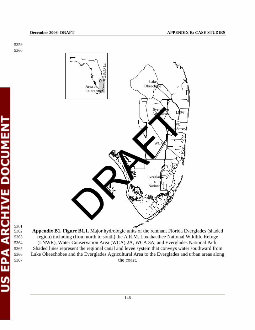
December 2006- DRAFT APPENDIX B: CASE STUDIES
146
5359 5360
5361 Appendix B1. Figure B1.1. Major hydrologic units of the remnant Florida Everglades (shaded 5362
region) including (from north to south) the A.R.M. Loxahacthee National Wildlife Refuge 5363 (LNWR), Water Conservation Area (WCA) 2A, WCA 3A, and Everglades National Park. 5364
Shaded lines represent the regional canal and levee system that conveys water southward from 5365 Lake Okeechobee and the Everglades Agricultural Area to the Everglades and urban areas along 5366
the coast. 5367
Everglades Agricultura
l
LNW
WCA
WCA
Everglades
National
Lake OkeechobeArea of
Enlargemen
FLOR
IDA
DRAFT
December 2006- DRAFT APPENDIX B: CASE STUDIES
147
smaller amounts of P via canal discharges into various parts of the Everglades. However, in 5368 general, canal P concentrations and loads (and associated wetland concentrations) decline from 5369 north to south . 5370 5371 The history of P enrichment and associated ecological impacts is not well documented, but 5372 probably occurred at a limited scale for much of the last century. Early reports by the South 5373 Florida Water Management District (e.g., Gleason et al. 1975, Swift and Nicholas 1987) showed 5374 an expansion of cattail and changes in the periphyton community in portions of the northern 5375 Everglades receiving EAA runoff. The severity and extent of P impacts were more fully 5376 recognized by 1988 when the Federal Government sued the State of Florida for allowing P-5377 enriched discharges and associated impacts to occur in the Everglades. Settlement of this 5378 lawsuit eventually resulted in the enactment of the Everglades Forever Act by the Florida 5379 Legislature in 1994, which required the Florida Department of Environmental Protection (FDEP) 5380 to derive a numeric water quality criterion for P that would “prevent ecological imbalances in 5381 natural populations of flora or fauna” in the Everglades. These legal and legislative events 5382 provided the basis for numerous research and monitoring efforts designed to better understand 5383 the effects of P enrichment and to determine levels of enrichment that produced undesirable 5384 ecosystem changes. 5385
5386 Research and monitoring were initiated by the State of Florida (the Florida Department of 5387 Environmental Protection and the South Florida Water Management District) and other 5388 university research groups (e.g., Duke University, Florida International University, University of 5389 Florida) to better understand ecological responses to anthropogenic P inputs and to identify a P 5390 concentration or range of concentrations that result in unacceptable degradation of the 5391 Everglades ecosystem. This case study reviews research and monitoring conducted by the State 5392 to derive a P criterion for the Everglades. This criterion was proposed by the FDEP in 2001 and 5393 approved in 2003. This process is divided into 3 parts: 5394 5395 1. Defining the reference (i.e., historical) conditions for P and the oligotrophic ecology of 5396
the Everglades; 5397 5398 2. Determine the types of ecological impacts caused by P enrichment; 5399 5400 3. Identify wetland P concentrations that produce these impacts, and determine a 5401
criterion that will protect the resource from those impacts. 5402 5403 5404 DEFINING THE REFERENCE CONDITION 5405 5406 Several sources of information were used to characterize reference conditions across the 5407 Everglades. Sampling in minimally impacted locations (i.e., reference sites) believed to best 5408 reflect historical conditions provided the quantitative basis for establishing reference conditions 5409
DRAFT

December 2006- DRAFT APPENDIX B: CASE STUDIES
148
with respect to P concentrations and associated ecological conditions. Where possible, this 5410 characterization was augmented by historical evidence. Written accounts of surveys conducted 5411 during the 1800s and early 1900s provided useful qualitative data on past ecological conditions. 5412 Early scientific literature contained substantial information on large-scale vegetation patterns 5413 (e.g., Davis 1943, Loveless 1959). Paleoecological assessments, including the dating and 5414 analysis of soil cores with respect to nutrient content and preserved materials such as pollen 5415 provided further information (e.g., Cooper and Goman 2001, Willard et al. 2001). 5416
5417 Predisturbance Everglades exhibited significant spatial and temporal variation, and, while its 5418 conversion to a smaller, more managed wetland resulted in the loss of some of this 5419 heterogeneity, the legacy of past variations in hydrology, chemistry, and biology remain in many 5420 areas. Legislation mandating the development of a P criterion stipulated that natural variation in 5421 P concentrations and ecological conditions within the remnant ecosystem be considered. This 5422 required that sampling efforts encompass the expected range of background variability in the 5423 remnant ecosystem. To ensure that spatial variation in P conditions were considered, sampling 5424 was conducted in all 4 major hydrologic units: The Loxahatchee National Wildlife Refuge 5425 (LNWR), WCA-2A, WCA-3A, and Everglades National Park (see Fig. 1). 5426 5427 Water Column Phosphorus 5428
5429 Nutrient inputs to the Everglades were historically derived primarily from atmospheric 5430 deposition (rainfall and dry fallout), which is typically low in P. Historical loading rates have 5431 been estimated from annual atmospheric P inputs in south Florida and reconstructions of P 5432 accumulation in Everglades soils and probably averaged less than 0.1 g P m-2 y-1 (SFWMD 5433 1992). Atmospheric inputs of P were augmented by inflows from Lake Okeechobee, which was 5434 connected by surface-water flows to the northern Everglades during periods of high water 5435 (Parker et al. 1955). While inflows from this historically eutrophic lake were undoubtedly 5436 enriched in P compared with the Everglades, the influence of these inputs were likely limited to 5437 wetlands along the lake’s southern fringe (Snyder and Davidson 1994) as is demonstrated by the 5438 limited extent of pond apple and other vegetation that require more nutrients for growth than the 5439 sawgrass (Cladium jamaicense) that dominates most of the Everglades. 5440
5441 Interior areas of the Everglades generally retain the oligotrophic characteristics of the 5442 predrainage ecosystem and, thus, provide the best contemporary information on historical P 5443 concentrations. Water chemistry data were available for several interior locations that had been 5444 sampled by the State for many years. Median water-column TP concentrations at these stations 5445 ranged between 4 and 10 µg L-1, with lowest concentrations occurring in southern areas that 5446 have been least affected by anthropogenic P loads (Fig. 3). Phosphorus concentrations >10 µg L-5447 1 were measured periodically at many of these sites. Isolated high P concentrations at reference 5448 stations were attributed to P released as a result of oxidation of exposed soils, increased fire 5449 frequency during droughts, and difficulties in collecting water samples that are not contaminated 5450 by flocculent wetland sediments when water depths are low. Data from reference sites may 5451
DRAFT
December 2006- DRAFT APPENDIX B: CASE STUDIES
149
represent an upper estimate of historical TP concentrations in the Everglades since several 5452 stations are located in areas that either have been overdrained, a condition which promotes soil 5453 oxidation and P release, or so heavily exposed to canal inflows (e.g., WCA 2A) that some P 5454 inputs have likely intruded even into interior areas. However, in the absence of reliable 5455 historical data, these values were deemed as best available for defining reference condition. 5456 5457 Soil Phosphorus 5458 5459 Extensive soil mapping projects across interior portions of the central and northern Everglades 5460 indicate a reference range for soil TP in the surface 0-10 cm of soil of between 200 and 500 mg 5461 kg-1 on a mass basis (DeBusk et al. 1994, Reddy et al. 1994a, Newman et al. 1997, Richardson et 5462 al. 1997a, Newman et al. 1998). Fewer data are available from ENP, but available evidence 5463 indicates background concentrations of < 400 mg kg-1 (Doren et al. 1997). Soil P content also 5464 varies volumetrically as a function of changing soil bulk density. The typical bulk density of 5465 flooded Everglades peat soils is approximately 0.08 g cm-3, whereas soils that have been 5466 subjected to extended dry out and oxidation can have bulk densities greater than 0.2 g cm-3 5467 (Newman et al. 1998). Increases in volumetric nutrient concentrations resulting from increased 5468 bulk density can have a stimulatory effect on plant growth even in the absence of external P 5469 inputs (see Chapter 2). Following correction for the varying bulk densities in the peat soils of 5470 the Everglades, a historical TP concentration of <40 µg cm-3 may be applicable for most regions 5471 (DeBusk et al. 1994, Reddy et al. 1994a, Newman et al. 1997, Newman et al. 1998, Reddy et al. 5472 1998). In the LNWR, most of the interior area has soil TP < 20 µg TP cm-3 (Newman et al. 5473 1997). 5474
DRAFT
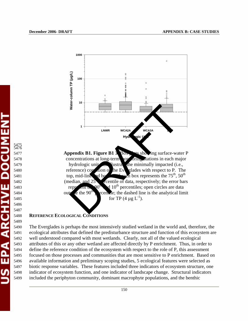
December 2006- DRAFT APPENDIX B: CASE STUDIES
150
Hydrologic Unit
Wat
er-c
olum
n TP
(µg/
L)
1
10
100
1000
LNWR WCA2A WCA3A ENP
5475 5476
Appendix B1. Figure B1 3. Box plots showing surface-water P 5477 concentrations at long-term monitoring stations in each major 5478
hydrologic unit that illustrate the minimally impacted (i.e., 5479 reference) condition of the Everglades with respect to P. The 5480 top, mid-line and bottom of each box represents the 75th, 50th 5481
(median, and 25th percentile of data, respectively; the error bars 5482 represent the 90th and 10th percentiles; open circles are data 5483
outside the 90th percentile; the dashed line is the analytical limit 5484 for TP (4 µg L-1). 5485
5486 5487
REFERENCE ECOLOGICAL CONDITIONS 5488 5489 The Everglades is perhaps the most intensively studied wetland in the world and, therefore, the 5490 ecological attributes that defined the predisturbance structure and function of this ecosystem are 5491 well understood compared with most wetlands. Clearly, not all of the valued ecological 5492 attributes of this or any other wetland are affected directly by P enrichment. Thus, in order to 5493 define the reference condition of the ecosystem with respect to the role of P, this assessment 5494 focused on those processes and communities that are most sensitive to P enrichment. Based on 5495 available information and preliminary scoping studies, 5 ecological features were selected as 5496 biotic response variables. These features included three indicators of ecosystem structure, one 5497 indicator of ecosystem function, and one indicator of landscape change. Structural indicators 5498 included the periphyton community, dominant macrophyte populations, and the benthic 5499
DRAFT
December 2006- DRAFT APPENDIX B: CASE STUDIES
151
macroinvertebrate community. Diel fluctuations in water column DO provided an important 5500 indicator of shifts in aquatic metabolism. The landscape indicator of change was the loss of 5501 open-water slough-wet prairie habitats--areas of high natural diversity and productivity. 5502 5503 Periphyton 5504 5505 Aquatic vegetation and other submerged surfaces in the oligotrophic Everglades interior are 5506 covered with periphyton, a community of algae, bacteria and other microorganisms. Periphyton 5507 accounts for a significant portion of primary productivity in sloughs and wet prairies (Wood and 5508 Maynard 1974, Browder et al. 1982, McCormick et al. 1998), and floating and attached 5509 periphyton mats provide an important habitat and food source for invertebrates and small fish 5510 (Browder et al. 1994, Rader 1994). These mats store large amounts of P (approaching 1 kg TP 5511 m-2 in some locations) and, thus, may play a critical role in maintaining low P concentrations in 5512 reference areas (McCormick et al. 1998, McCormick and Scinto 1999). Periphyton biomass and 5513 productivity peak towards the end of the wet season (August through October) and reach a 5514 minimum during the colder months of the dry season (January through March). Periphyton 5515 biomass in open-water habitats can exceed 1 kg m-2 during the wet season (Wood and Maynard 5516 1974, Browder et al. 1982, McCormick et al. 1998) when floating mats can become so dense as 5517 to cover the entire water surface. Aerobic conditions in slough-wet prairie habitats is maintained 5518 by the high productivity of this community and the capacity of dense algal mats to trap oxygen 5519 released during photosynthesis (McCormick and Laing 2003). 5520 5521 Two types of periphyton communities occur in reference areas of the Everglades. Mineral-rich 5522 waters, such as those found WCA 2A and Taylor Slough (ENP), support a periphyton 5523 assemblage dominated by a few species of calcium-precipitating cyanobacteria and diatoms, 5524 while the soft-water interior of LNWR contain a characteristic assemblage of desmid green algae 5525 and diatoms. Waters across much of the southern Everglades (WCA-3A and portions of ENP) 5526 tend to be intermediate with respect to mineral content and contain some taxa from both 5527 assemblages. 5528 5529 The chemical composition of periphyton in the oligotrophic Everglades is indicative of severe P 5530 limitation. Periphyton samples from reference areas of major hydrologic units within the 5531 Everglades are characterized by an extremely low P content (generally <0.05%) and extremely 5532 high N:P ratios (generally >60:1 w:w). This observational evidence for P limitation is supported 5533 by experimental fertilization studies that have shown that: 1) periphyton responds more strongly 5534 to P enrichment than to enrichment with other commonly limiting nutrients such as nitrogen 5535 (Scheidt et al. 1989, Vymazal et al. 1994); 2) periphyton changes in response to experimental P 5536 enrichment mimic those that occur along field nutrient gradients (McCormick and O’Dell 1996). 5537 Thus, it is well-established that periphyton is strongly P-limited in reference areas of the 5538 Everglades. 5539 5540 Dissolved Oxygen 5541
DRAFT
December 2006- DRAFT APPENDIX B: CASE STUDIES
152
5542 Interior Everglades habitats exhibit characteristic diel fluctuations in water-column dissolved 5543 oxygen (DO), although aerobic conditions are generally maintained throughout much or all of 5544 the diel cycle (Belanger et al. 1989, McCormick et al. 1997, McCormick and Laing 2003). High 5545 daytime concentrations in open-water habitats (i.e., sloughs, wet prairies) are a product of 5546 photosynthesis by periphyton and other submerged vegetation. These habitats may serve as 5547 oxygen sources for adjacent sawgrass stands, where submerged productivity is low (Belanger et 5548 al. 1989). Oxygen concentrations decline rapidly during the night due to periphyton and 5549 sediment microbial respiration and generally fall below the 5 mg L-1 standard for Class III 5550 Florida waters (Criterion 17-302.560(21), F.A.C.). However, these diurnal excursions are 5551 characteristic of reference areas throughout the Everglades (McCormick et al. 1997) and are not 5552 considered a violation of the Class III standard (Nearhoof 1992). 5553
Vegetation 5554 5555 The vegetation communities characteristic of the pristine Everglades are dominated by species 5556 adapted to low P, seasonal patterns of wetting and drying, and periodic natural disturbances such 5557 as fire, drought and occasional freezes (Duever et al. 1994, Davis 1943, Steward and Ornes 5558 1983, Parker 1974). Major aquatic vegetation habitats in oligotrophic areas include sawgrass 5559 wetlands, wet prairies, and sloughs (Loveless 1959, Gunderson 1994). The spatial arrangement 5560 of these habitats is dynamic and controlled by environmental factors such as fire, water depth, 5561 nutrient availability and local topography (Loveless 1959). 5562 5563 Sawgrass (Cladium jamaicense) is the dominant macrophyte in the Everglades, and stands of this 5564 species compromise approximately 65 to 70% of the total vegetation cover of the Everglades 5565 (Loveless 1959). Wet prairies include a collection of low-stature, graminoid communities 5566 occurring on both peat and marl soils (Gunderson 1994). Dominant macrophyte taxa in these 5567 habitats include Rhynchospora, Panicum and Eleocharis (Loveless 1959, Craighead 1971). 5568 Sloughs are deeper water habitats that remain wet most or all of the year and are characterized 5569 by floating macrophytes such as fragrant white water lily (Nymphaea odorata), floating hearts 5570 (Nymphoides Aquaticum) and spatterdock (Nuphar advena) (Loveless 1959, Gunderson 1994). 5571 Submerged aquatic plants, primarily bladderworts (Utricularia foliosa and U. purpurea in 5572 particular), also can be abundant in these habitats and, in the case of U. purpurea, provide a 5573 substrate for the formation of dense periphyton mats. 5574 5575
DRAFT
December 2006- DRAFT APPENDIX B: CASE STUDIES
153
Several studies have concluded that macrophyte communities in the Everglades are P-limited. 5576 Sawgrass is adapted to the low-P conditions indicative of the pristine Everglades (Steward and 5577 Ornes 1975b, Steward and Ornes 1983). During field and greenhouse manipulations, sawgrass 5578 responded to P enrichment either by increasing the rate of growth or P uptake (Steward and 5579 Ornes 1975a, Steward and Ornes 1983, Craft et al. 1995, Miao et al. 1997, Daoust and Childers 5580 1999). Furthermore, additions of N alone had no effect on sawgrass or cattail growth under low-5581 P conditions (Steward and Ornes 1983, Craft et al. 1995). Recent experimental evidence in the 5582 Everglades National Park (Daoust and Childers 1999) has shown that other native vegetation 5583 associations such as wet prairie communities are also limited by P. 5584 5585 Historically, cattail (Typha spp.) was one of several minor macrophyte species native to the 5586 Everglades (Davis 1943, Loveless 1959). In particular, cattail is believed to have been 5587 associated largely with areas of disturbance such as alligator holes and recent burns (Davis 5588 1994). Analyses of Everglades peat deposits reveal no evidence of cattail peat although the 5589 presence of cattail pollen indicates its presence historically in some areas (Gleason and Stone 5590 1994, Davis et al. 1994, Bartow et al. 1996). Findings such as these confirm the historical 5591 presence of cattail in the Everglades but provide no evidence for the existence of dense cattail 5592 stands covering large areas (Wood and Tanner 1990) as now occurs in the northern Everglades. 5593 In contrast, sawgrass and water lily peats have been major freshwater Everglades soils for 5594 approximately 4,000 years (McDowell et al. 1969). 5595
Macroinvertebrates 5596 5597 Aquatic invertebrates (e.g., insects, snails, and crayfish) represent a key intermediate position in 5598 energy flow through the Everglades food web as these taxa are the direct consumers of primary 5599 production and, in turn, are consumed by vertebrate predators. Invertebrates occupy several 5600 functional niches within the Everglades food web; however, most taxa are direct consumers of 5601 periphyton and/or plant detritus (e.g., Rader and Richardson 1994, McCormick et al. 2004). 5602 Rader (1994) sampled both periphyton and macrophyte habitats in this same area and, based on 5603 the proportional abundance of different functional groups, suggested that grazer (periphyton) and 5604 detrital (plant) pathways contributed equally to energy flow in low-nutrient areas of the 5605 Everglades. 5606 5607 The macroinvertebrate fauna of the Everglades is fairly diverse (approximately 200 taxa 5608 identified) and is dominated by Diptera (49 taxa), Coleoptera (48 taxa), Gastropoda (17 taxa) 5609 Odonata (14 taxa), and Oligochaeta (11 taxa) (Rader 1999). Most studies have focused on a few 5610 conspicuous species (e.g., crayfish and apple snails) considered to be of special importance to 5611 vertebrate predators, and relatively little is known about the distribution and environmental 5612 tolerances of most taxa. An assemblage of benthic microinvertebrates (meiofauna) dominated by 5613 Copepoda and Cladocera is also present in the Everglades (Loftus et al. 1986), but even less is 5614 known about the distribution and ecology of these organisms. 5615 5616
DRAFT
December 2006- DRAFT APPENDIX B: CASE STUDIES
154
Invertebrates are not distributed evenly among Everglades habitats but, instead, tend to be 5617 concentrated in periphyton-rich habitats such as sloughs. In an early study, Reark (1961) noted 5618 that invertebrate densities in ENP were higher in periphyton habitats compared with sawgrass 5619 stands. Rader (1994) reported similar findings in the northern Everglades and found mean 5620 annual invertebrate densities to be more than six-fold higher in sloughs than in sawgrass stands. 5621 Invertebrate assemblages in sloughs were more species-rich and contained considerably higher 5622 densities of most dominant invertebrate groups. Functionally, slough invertebrate assemblages 5623 contained similar densities of periphyton grazers and detritivores, compared with a detritivore-5624 dominated assemblage in sawgrass stands. Higher invertebrate densities in sloughs were 5625 attributed primarily to abundant growths of periphyton and submerged vegetation, which provide 5626 oxygen and a source of high- quality food. 5627 5628 5629 QUANTIFYING P IMPACTS 5630 5631 A targeted design (see Chapter 4 of this document) was used to quantify changes in key 5632 ecological attributes in response to P enrichment Discharges of canal waters through fixed 5633 water-control structures are the primary source of anthropogenic P for the Everglades and 5634 produce P gradients that extend several kilometers into the wetland in several locations. These 5635 gradients have existed for several decades and provided the clearest example of the long-term 5636 ecological impacts associated with P enrichment. Monitoring was conducted along gradients in 5637 different parts of the Everglades to assess ecological responses to P enrichment. Fixed sampling 5638 stations were located along the full extent of each gradient to document ecological conditions 5639 associated with increasing levels of P enrichment. Intensive monitoring was performed along 5640 gradients in two northern Everglades wetlands, WCA 2A and the LNWR. WCA 2A is a 5641 mineral-rich, slightly basic peatland and contains the most pronounced and well studied P 5642 gradient in the Everglades, whereas LNWR is a soft-water, slightly acidic peatland. These two 5643 wetlands represent the most extreme natural water chemistry conditions in the Everglades and 5644 support distinct periphyton assemblages and macrophyte populations while sharing dominant 5645 species such as sawgrass and water lily. Less intensive sampling along gradients in other parts 5646 of the Everglades (WCA 3A and ENP) to confirm that P relationships were consistent across the 5647 wetland. 5648 5649 Chemical and biological conditions were measured at each sampling station along the two 5650 intensively sampled gradients. Repeated sampling, sometimes over several years was performed 5651 to ensure that temporal variation in each metric was considered in the final data analysis. 5652 Monthly surface-water sampling and less frequent soil sampling were performed to quantify P 5653 gradients in each area. Diel DO regimes, periphyton, and benthic macroinvertebrates were 5654 sampled quarterly when surface water was present. Macrophyte sampling included ground-5655 based methods to document shifts in species composition and remote sensing to determine 5656 changes in landscape patterns. The hydrology of each site was characterized to determine 5657
DRAFT
December 2006- DRAFT APPENDIX B: CASE STUDIES
155
whether P gradients were confounded with hydrologic gradients, which can also exert a strong 5658 influence on ecological patterns. 5659
5660 Numerous field experiments have been conducted to quantify ecological responses to P 5661 enrichment and to better understand how interactions between P enrichment and other factors 5662 such as hydrology may affect these responses. The design of these experiments varied in 5663 complexity with respect to size and dosing regime depending on the specific objective of each 5664 study and has included enclosed fertilizer plots (e.g., Craft et al. 1995), semi-permeable 5665 mesocosms receiving periodic P additions to achieve fixed loading rates in the form of periodic 5666 additions (e.g., McCormick and O’Dell 1996), flumes receiving semi-continuous enrichment at a 5667 fixed rate (Pan et al. 2000), and flumes receiving flow-adjusted dosing to achieve constant 5668 inflow concentrations (Childers et al. 2002). These experiments were useful in establishing the 5669 causal nature of responses to P enrichment documented along the P gradients described above. 5670 5671 5672
GRADIENT P CONCENTRATIONS 5673
Strong gradients in P concentrations were documented downstream of canal discharges into most 5674 Everglades wetlands (Fig. 4). Inflow TP concentrations in from 1996-1999 have averaged as 5675 high as 100 µg L-1 as compared with reference and pre-disturbance concentrations < 10 µg L-1 . 5676 The degree and spatial extent of P enrichment varies among areas depending on the source and 5677 magnitude of inflows. The most extensive enrichment has occurred in the northern Everglades 5678 near EAA inflows, while southern areas (e.g., ENP) have been relatively less affected. The most 5679 extensive enrichment has occurred in WCA-2A, which, unlike other areas, receives most of its 5680 water from canal discharges. Soil TP was strongly correlated with surface-water concentrations 5681 and exceeded 1500 mg kg-1 at the most enriched locations as compared with concentrations < 5682 500 mg kg-1 in reference areas. In general, this enrichment effect is limited to the surface 30 cm 5683 of soil depth (Reddy et al. 1998). 5684 DRAFT
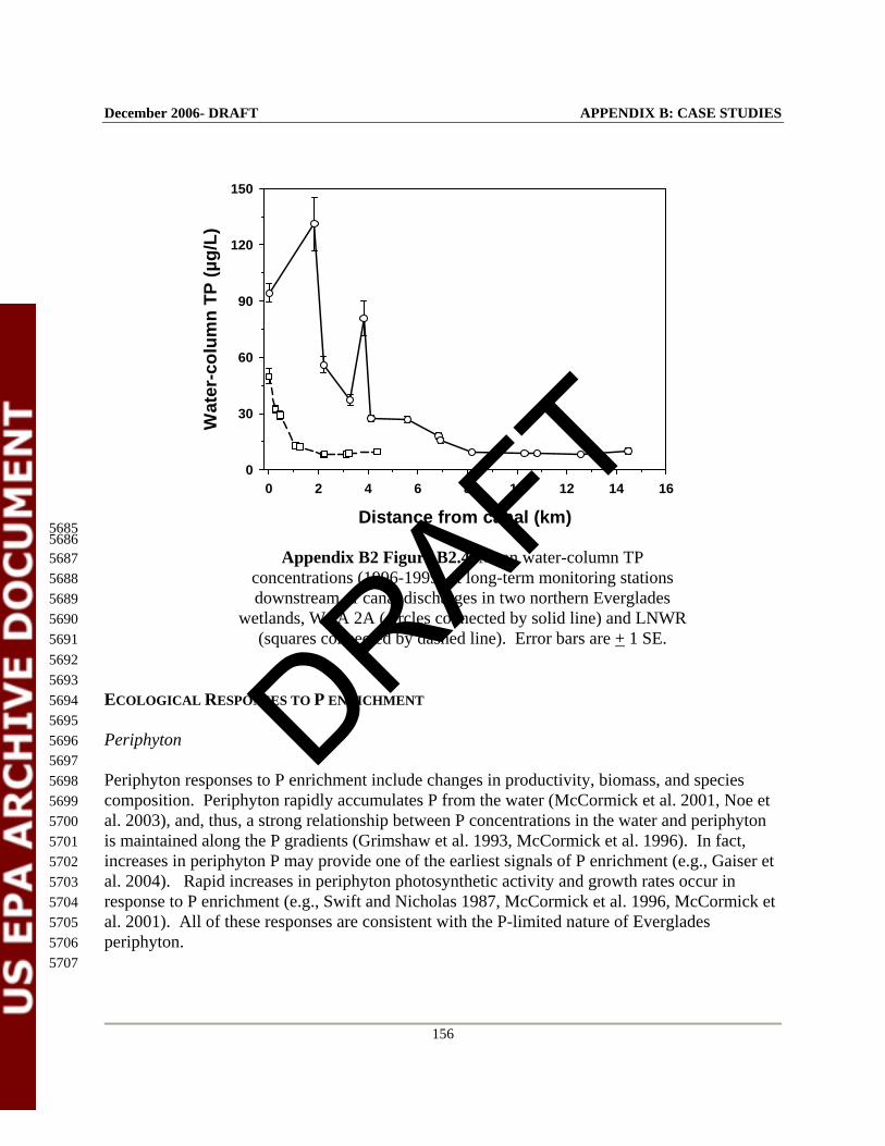
December 2006- DRAFT APPENDIX B: CASE STUDIES
156
Distance from canal (km)0 2 4 6 8 10 12 14 16
Wat
er-c
olum
n TP
(µg/
L)
0
30
60
90
120
150
5685 5686
Appendix B2 Figure B2.4. Mean water-column TP 5687 concentrations (1996-1999) at long-term monitoring stations 5688 downstream of canal discharges in two northern Everglades 5689
wetlands, WCA 2A (circles connected by solid line) and LNWR 5690 (squares connected by dashed line). Error bars are + 1 SE. 5691
5692 5693 ECOLOGICAL RESPONSES TO P ENRICHMENT 5694 5695 Periphyton 5696 5697 Periphyton responses to P enrichment include changes in productivity, biomass, and species 5698 composition. Periphyton rapidly accumulates P from the water (McCormick et al. 2001, Noe et 5699 al. 2003), and, thus, a strong relationship between P concentrations in the water and periphyton 5700 is maintained along the P gradients (Grimshaw et al. 1993, McCormick et al. 1996). In fact, 5701 increases in periphyton P may provide one of the earliest signals of P enrichment (e.g., Gaiser et 5702 al. 2004). Rapid increases in periphyton photosynthetic activity and growth rates occur in 5703 response to P enrichment (e.g., Swift and Nicholas 1987, McCormick et al. 1996, McCormick et 5704 al. 2001). All of these responses are consistent with the P-limited nature of Everglades 5705 periphyton. 5706 5707
DRAFT
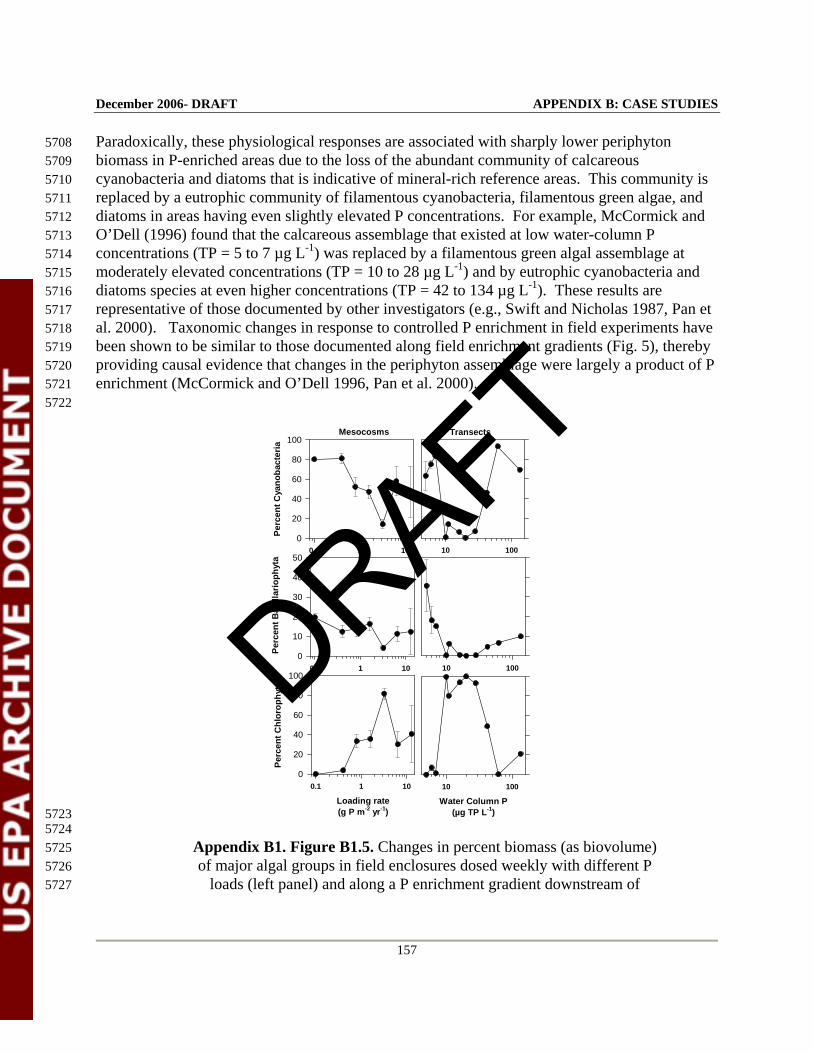
December 2006- DRAFT APPENDIX B: CASE STUDIES
157
Paradoxically, these physiological responses are associated with sharply lower periphyton 5708 biomass in P-enriched areas due to the loss of the abundant community of calcareous 5709 cyanobacteria and diatoms that is indicative of mineral-rich reference areas. This community is 5710 replaced by a eutrophic community of filamentous cyanobacteria, filamentous green algae, and 5711 diatoms in areas having even slightly elevated P concentrations. For example, McCormick and 5712 O’Dell (1996) found that the calcareous assemblage that existed at low water-column P 5713 concentrations (TP = 5 to 7 µg L-1) was replaced by a filamentous green algal assemblage at 5714 moderately elevated concentrations (TP = 10 to 28 µg L-1) and by eutrophic cyanobacteria and 5715 diatoms species at even higher concentrations (TP = 42 to 134 µg L-1). These results are 5716 representative of those documented by other investigators (e.g., Swift and Nicholas 1987, Pan et 5717 al. 2000). Taxonomic changes in response to controlled P enrichment in field experiments have 5718 been shown to be similar to those documented along field enrichment gradients (Fig. 5), thereby 5719 providing causal evidence that changes in the periphyton assemblage were largely a product of P 5720 enrichment (McCormick and O’Dell 1996, Pan et al. 2000). 5721 5722
Loading rate(g P m-2 yr-1)
0.1 1 10
Perc
ent C
hlor
ophy
ta
0
20
40
60
80
100
Water Column P(µg TP L-1)
10 100
TransectsMesocosms
0.1 1 10
Perc
ent C
yano
bact
eria
0
20
40
60
80
100
10 100
0.1 1 10
Perc
ent B
acill
ario
phyt
a
0
10
20
30
40
50
10 100
5723 5724
Appendix B1. Figure B1.5. Changes in percent biomass (as biovolume) 5725 of major algal groups in field enclosures dosed weekly with different P 5726
loads (left panel) and along a P enrichment gradient downstream of 5727
DRAFT
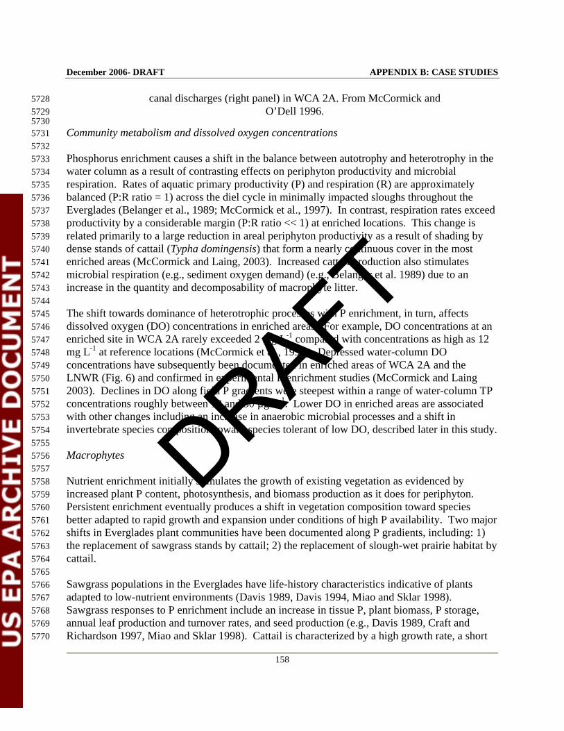
December 2006- DRAFT APPENDIX B: CASE STUDIES
158
canal discharges (right panel) in WCA 2A. From McCormick and 5728 O’Dell 1996. 5729
5730 Community metabolism and dissolved oxygen concentrations 5731 5732 Phosphorus enrichment causes a shift in the balance between autotrophy and heterotrophy in the 5733 water column as a result of contrasting effects on periphyton productivity and microbial 5734 respiration. Rates of aquatic primary productivity (P) and respiration (R) are approximately 5735 balanced (P:R ratio = 1) across the diel cycle in minimally impacted sloughs throughout the 5736 Everglades (Belanger et al., 1989; McCormick et al., 1997). In contrast, respiration rates exceed 5737 productivity by a considerable margin (P:R ratio << 1) at enriched locations. This change is 5738 related primarily to a large reduction in areal periphyton productivity as a result of shading by 5739 dense stands of cattail (Typha domingensis) that form a nearly continuous cover in the most 5740 enriched areas (McCormick and Laing, 2003). Increased cattail production also stimulates 5741 microbial respiration (e.g., sediment oxygen demand) (e.g., Belanger et al. 1989) due to an 5742 increase in the quantity and decomposability of macrophyte litter. 5743 5744 The shift towards dominance of heterotrophic processes with P enrichment, in turn, affects 5745 dissolved oxygen (DO) concentrations in enriched areas. For example, DO concentrations at an 5746 enriched site in WCA 2A rarely exceeded 2 mg L-1 compared with concentrations as high as 12 5747 mg L-1 at reference locations (McCormick et al., 1997). Depressed water-column DO 5748 concentrations have subsequently been documented in enriched areas of WCA 2A and the 5749 LNWR (Fig. 6) and confirmed in experimental P-enrichment studies (McCormick and Laing 5750 2003). Declines in DO along field P gradients were steepest within a range of water-column TP 5751 concentrations roughly between 10 and 30 µg L-1. Lower DO in enriched areas are associated 5752 with other changes including an increase in anaerobic microbial processes and a shift in 5753 invertebrate species composition toward species tolerant of low DO, described later in this study. 5754 5755 Macrophytes 5756 5757 Nutrient enrichment initially stimulates the growth of existing vegetation as evidenced by 5758 increased plant P content, photosynthesis, and biomass production as it does for periphyton. 5759 Persistent enrichment eventually produces a shift in vegetation composition toward species 5760 better adapted to rapid growth and expansion under conditions of high P availability. Two major 5761 shifts in Everglades plant communities have been documented along P gradients, including: 1) 5762 the replacement of sawgrass stands by cattail; 2) the replacement of slough-wet prairie habitat by 5763 cattail. 5764
5765 Sawgrass populations in the Everglades have life-history characteristics indicative of plants 5766 adapted to low-nutrient environments (Davis 1989, Davis 1994, Miao and Sklar 1998). 5767 Sawgrass responses to P enrichment include an increase in tissue P, plant biomass, P storage, 5768 annual leaf production and turnover rates, and seed production (e.g., Davis 1989, Craft and 5769 Richardson 1997, Miao and Sklar 1998). Cattail is characterized by a high growth rate, a short 5770
DRAFT
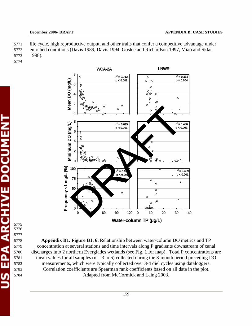
December 2006- DRAFT APPENDIX B: CASE STUDIES
159
life cycle, high reproductive output, and other traits that confer a competitive advantage under 5771 enriched conditions (Davis 1989, Davis 1994, Goslee and Richardson 1997, Miao and Sklar 5772 1998). 5773 5774
WCA-2AM
ean
DO
(mg/
L)
0
2
4
6
8
0 10 20 30 40
r2 = 0.489p < 0.001
Water-column TP (µg/L)0 30 60 90 120
Freq
uenc
y <1
mg/
L (%
)
0
25
50
75
100r2 = 0.692p < 0.001
r2 = 0.436p < 0.001
LNWR
r2 = 0.314p = 0.004
r2 = 0.712p < 0.001
Min
imum
DO
(mg/
L)
0
2
4
6
8r2 = 0.615p < 0.001
5775 5776
5777 Appendix B1. Figure B1. 6. Relationship between water-column DO metrics and TP 5778
concentration at several stations and time intervals along P gradients downstream of canal 5779 discharges into 2 northern Everglades wetlands (see Fig. 1 for map). Total P concentrations are 5780
mean values for all samples (n = 3 to 6) collected during the 3-month period preceding DO 5781 measurements, which were typically collected over 3-4 diel cycles using dataloggers. 5782 Correlation coefficients are Spearman rank coefficients based on all data in the plot. 5783
Adapted from McCormick and Laing 2003. 5784
DRAFT
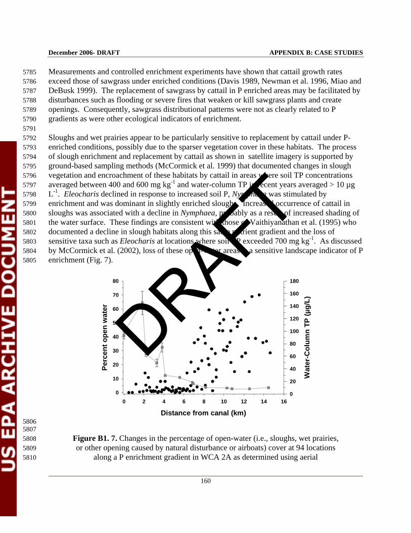
December 2006- DRAFT APPENDIX B: CASE STUDIES
160
Measurements and controlled enrichment experiments have shown that cattail growth rates 5785 exceed those of sawgrass under enriched conditions (Davis 1989, Newman et al. 1996, Miao and 5786 DeBusk 1999). The replacement of sawgrass by cattail in P enriched areas may be facilitated by 5787 disturbances such as flooding or severe fires that weaken or kill sawgrass plants and create 5788 openings. Consequently, sawgrass distributional patterns were not as clearly related to P 5789 gradients as were other ecological indicators of enrichment. 5790
5791 Sloughs and wet prairies appear to be particularly sensitive to replacement by cattail under P-5792 enriched conditions, possibly due to the sparser vegetation cover in these habitats. The process 5793 of slough enrichment and replacement by cattail as shown in satellite imagery is supported by 5794 ground-based sampling methods (McCormick et al. 1999) that documented changes in slough 5795 vegetation and encroachment of these habitats by cattail in areas where soil TP concentrations 5796 averaged between 400 and 600 mg kg-1 and water-column TP in recent years averaged > 10 µg 5797 L-1. Eleocharis declined in response to increased soil P, Nymphaea was stimulated by 5798 enrichment and was dominant in slightly enriched sloughs. Increased occurrence of cattail in 5799 sloughs was associated with a decline in Nymphaea, probably as a result of increased shading of 5800 the water surface. These findings are consistent with those of Vaithiyanathan et al. (1995) who 5801 documented a decline in slough habitats along this same nutrient gradient and the loss of 5802 sensitive taxa such as Eleocharis at locations where soil TP exceeded 700 mg kg-1. As discussed 5803 by McCormick et al. (2002), loss of these open-water areas is a sensitive landscape indicator of P 5804 enrichment (Fig. 7). 5805
Distance from canal (km)0 2 4 6 8 10 12 14 16
Perc
ent o
pen
wat
er
0
10
20
30
40
50
60
70
80
Wat
er-C
olum
n TP
(µg/
L)
0
20
40
60
80
100
120
140
160
180
5806 5807
Figure B1. 7. Changes in the percentage of open-water (i.e., sloughs, wet prairies, 5808 or other opening caused by natural disturbance or airboats) cover at 94 locations 5809
along a P enrichment gradient in WCA 2A as determined using aerial 5810
DRAFT
December 2006- DRAFT APPENDIX B: CASE STUDIES
161
photography. Gray line shows the mean (+ 1 SE) water-column TP concentration 5811 (1996-1999) at 15 long-term monitoring stations along the gradient. 5812
5813 Benthic Macroinvertebrates 5814
5815 Macroinvertebrates are the most widely used biological indicator of water quality impacts, and 5816 several changes that occur in this community along P enrichment gradients in the Everglades are 5817 similar to those documented in response to eutrophication in other aquatic ecosystems. Several 5818 studies have documented an overall increase in macroinvertebrate abundance with increasing P 5819 enrichment (Rader and Richardson 1994, Trexler and Turner et al. 1999, McCormick et al. 5820 2004). However, differences in sampling methodology have apparently produced conflicting 5821 results with respect to changes in species richness and diversity. For example, Rader and 5822 Richardson (1994) documented an increase in both macroinvertebrate species richness and 5823 diversity with P enrichment in open-water (i.e., low emergent macrophyte cover) habitats and 5824 concluded that enrichment had not impacted this community. McCormick et al. (2004) however, 5825 using a landscape approach that involved habitat-weighted sampling, found little change in either 5826 species richness or diversity in response to enrichment. This latter study accounted for the 5827 decline in the cover of habitats such as sloughs and wet prairies, which contain the most diverse 5828 and abundant macroinvertebrate communities (Rader 1994). McCormick et al. (2004) also 5829 documented a pronounced shift in community composition with increasing P enrichment as taxa 5830 characteristic of the oligotrophic interior of the wetland are replaced by common pollution-5831 tolerant taxa of oligochaetes and chironomids. These changes were indicative of habitat 5832 degradation as determined using biotic indices derived by the Florida DEP to assess stream 5833 condition based on macroinvertebrate composition (results available at 5834 http://www.epa.gov/owow/wetlands/bawwg/case/fl2.html). 5835
5836 As for many other P-induced biological changes, the greatest change in the macroinvertebrate 5837 community occurred in response to relatively small increases in P concentration. Along field 5838 enrichment gradients, community shifts were associated with increases in water-column TP 5839 above approximately 10 ug L-1 (McCormick et al. 2004). Similarly, Qian et al. (2004) 5840 documented several shifts in community structure and function in response to long-term 5841 experimental dosing at average concentrations of approximately 10-15 ug L-1. 5842 5843 ESTABLISHING A P CRITERION 5844 5845 The FDEP was charged with reviewing and analyzing available P and ecological data collected 5846 throughout the Everglades to establish a numeric P criterion. A brief summary of this process is 5847 provided here and more detailed can be found in Payne et al (2002, 2003; both available at 5848 http://www.sfwmd.gov/sfer/previous_ecr.html). 5849 5850 The narrative nutrient standard for Class III Florida waters such as the Everglades states that “in 5851 no case shall nutrient concentrations of a body of water be altered so as to cause an imbalance in 5852 natural populations of aquatic flora and fauna.” The FDEP approach to detecting violations of 5853
DRAFT
December 2006- DRAFT APPENDIX B: CASE STUDIES
162
this standard with respect to surface-water P concentrations in the Everglades was to test for 5854 statistically significant departures in ecological conditions from those at reference sites, i.e., 5855 interior sampling locations with background P concentrations. Biological and chemical data 5856 collected along anthropogenic P gradients throughout the Everglades were analyzed to determine 5857 P concentrations associated with such departures. Results showed that sampling sites with 5858 average (geometric mean) surface-water TP concentrations significantly greater than 10 ppb 5859 consistently exhibited significant departures in ecological condition from that of reference sites. 5860 A key finding supporting this concentration as the standard was the fact that multiple changes in 5861 each of the major indicator groups – periphyton, dissolved oxygen, macrophytes, and 5862 macroinvertebrates – all occurred at or near this same concentration (e.g., Payne et al. 2001). 5863 5864 Data from field and laboratory experiments conducted by various research groups provided 5865 valuable supporting information for understanding responses to P enrichment. While such 5866 experiments were not used directly to derive the P criterion, they established cause-effect 5867 relationships between P enrichment and ecological change that supported correlative 5868 relationships documented along field P gradients. For example, McCormick and O’Dell (1996) 5869 and Pan et al. (2000) showed that major shifts in periphyton species composition documented 5870 along field P gradients matched those elicited by controlled P dosing in field enrichment 5871 experiments. McCormick and Laing (2003) confirmed that controlled P enrichment produced 5872 declines in water-column DO similar to those measured along the gradients. Macroinvertebrate 5873 community changes were documented experimentally Qian et al. (2004). 5874 5875 While the criterion established a surface-water concentration of 10 ug L-1 TP as protective of 5876 native flora and fauna, the methodology used to measure compliance with the criterion needed to 5877 normalize background fluctuations in concentration. Additional analyses of P data collected 5878 over several years at reference sites was used to set both a longer-term average concentration and 5879 a shorter-term maximum concentration for each site. Based on these analyses, the FDEP 5880 concluded that annual maximum concentrations at a given sampling location should not exceed 5881 15 ug L-1 TP while long-term while 5-year average concentrations should not exceed 10 ug L-1 5882 TP. These limits would be applied to reference areas to ensure no further degradation and to 5883 areas already impacted by P enrichment to gauge the rate and extent of recovery in response to a 5884 suite of P control measures including agricultural BMPs and the construction of treatment 5885 wetlands to remove P from surface runoff prior to being discharged into the Everglades. 5886 5887
DRAFT
December 2006- DRAFT APPENDIX B: CASE STUDIES
163
LITERATURE CITED 5888 5889 Bartow, S. M., Craft, C. B., and Richardson, C. J., Reconstructing historical changes in 5890
Everglades plant community composition using pollen distributions in peat, Journal of 5891 Lake and Reservoir Management, 12, 313, 1996. 5892
5893 Belanger, T. V., Scheidt, D. J., and Platko, J. R. II., Effects of nutrient enrichment on the Florida 5894
Everglades, Lake and Reservoir Management, 5, 101, 1989. 5895 5896 Browder, J.A., Cottrell, D., Brown, M., Newman, M., Edwards, R., Yuska, J., Browder, M., and 5897
Krakoski, J., Biomass and Primary Production of Microphytes and Macrophytes in 5898 Periphyton Habitats of the Southern Everglades, Report T-662, South Florida Research 5899 Center, Homestead, FL., 1982. 5900
5901 Browder, J. A., Gleason, P. J., and Swift, D. R., Periphyton in the Everglades: spatial variation, 5902
environmental correlates, and ecological implications, in Everglades: The Ecosystem and 5903 It’s Restoration, Davis, S. M. and Ogden, J. C., Eds., St. Lucie Press, Delray Beach, 5904 Florida, 1994, 379. 5905
5906 Childers, D.L., R.D. Jones, J.C. Trexler, C. Buzzelli, S. Dailey, A.L. Edwards, E.E. Gaiser, K. 5907
Jayachandaran, A. Kenne, D. Lee, J.F. Meeder, J.H.K. Pechman, A. Renshaw, J. 5908 Richards, M. Rugge, L.J. Scinto, P. Sterling, and W. Van Gelder, 2002. Quantifying the 5909 effects of low level phosphorus enrichment on unimpacted Everglades wetlands with in 5910 situ flumes and phosphorus dosing. In Porter, J. and Porter, K. (eds). The Everglades, 5911 Florida Bay and Coral Reefs of the Florida Keys: An Ecosystem Sourcebook. CRC 5912 Press. Boca Raton, FL. Pages 127-152. 5913
5914 Cooper, S. R., and Goman, M., Historical changes in water quality and vegetation in WCA-2A 5915
as determined by paleoecological analyses, in An Integrated Approach to Wetland 5916 Ecosystem Science: The Everglades Experiments, Richardson, C. J., Ed., Springer-5917 Verlag, New York, 2001, in press. 5918
5919 Craft, C. B., Vymazal, J., and Richardson, C. J., Response of Everglades plant communities to 5920
nitrogen and phosphorus additions, Wetlands, 15, 258, 1995. 5921 5922 Craft, C. B., and Richardson, C. J., Relationships between soil nutrients and plant species 5923
composition in Everglades peatlands, Journal of Environmental Quality, 26, 224, 1997. 5924 5925 Craighead, F. C., The Trees of South Florida Vol I: The Natural Environments and Their 5926
Succession, University of Miami Press, Coral Gables, Florida, 1971. 5927 5928
DRAFT

December 2006- DRAFT APPENDIX B: CASE STUDIES
164
Daoust, R. J., and Childers, D. L., Controls on emergent macrophyte composition, abundance, 5929 and productivity in freshwater Everglades wetland communities, Wetlands, 19, 262, 5930 1999. 5931
5932 Davis, J. H., Jr., The Natural Features of South Florida, Especially the Vegetation, and the 5933
Everglades, Bulletin No. 25, Florida Geological Survey, 1943. 5934 5935 Davis, S. M., Sawgrass and cattail production in relation to nutrient supply in the Everglades, in 5936
Freshwater Wetlands and Wildlife, Sharitz, R. R., and Gibbons, J. W., Eds., USDOE 5937 Office of Scientific and Technical Information, Oak Ridge, Tennessee, 1989, 325. 5938
5939 Davis, S. M., Gunderson, L. H., Park, W. A., Richardson, J., and Mattson, J., Landscape 5940
dimension, composition, and function in a changing Everglades ecosystem, in 5941 Everglades: The Ecosystem and It’s Restoration, Davis, S. M., and Ogden, J. C., Eds., St. 5942 Lucie Press, Delray Beach, Florida, 1994, 419. 5943
5944 DeBusk, W. F., Reddy, K. R., Koch, M. S., and Wang, Y., Spatial distribution of soil nutrients in 5945
a northern Everglades marsh - Water Conservation Area 2A, Soil Science Society of 5946 America Journal, 58, 543, 1994. 5947
5948 Doren, R. F., Armentano, T. V., Whiteaker, L. D., and Jones, R. D., Marsh vegetation patterns 5949
and soil phosphorus gradients in the Everglades ecosystem. Aquatic Botany, 56, 145, 5950 1997. 5951
5952 Duever, M. J., Meeder, J. F., Meeder, L. C., and McCollom, J. M., The climate of south Florida 5953
and its role in shaping the Everglades ecosystem, in Everglades: The Ecosystem and It’s 5954 Restoration, Davis, S. M. and Ogden, J. C., Eds., St. Lucie Press, Delray Beach, Florida, 5955 1994, 225. 5956
5957 Gaiser, E.E., L.J. Scinto, J.H. Richards, K. Jayachandran, D.L. Childers, J.C. Trexler, and R.D. 5958
Jones. 2004. Phosphorus in periphyton mats provides the best metric for detecting low-5959 level P enrichment in an oligotrophic wetland. Water Research 38:507-516. 5960
5961 Gleason, P. J., Stone, P. A., Age, origin, and evolution of the Everglades peatland, in 5962
Everglades: The Ecosystem and It’s Restoration, Davis, S. M. and Ogden, J. C., Eds., St. 5963 Lucie Press, Delray Beach, Florida, 1994, 149. 5964
5965 Gleason, P. J., Stone, P. A., Hallett, D., and Rosen, M., Preliminary report on the effect of 5966
agricultural runoff on the periphytic algae of Conservation Area 1, Unpublished report, 5967 Central and Southern Flood Control District, West Palm Beach, FL, 1975. 5968
5969
DRAFT
December 2006- DRAFT APPENDIX B: CASE STUDIES
165
Goslee, S. C., and Richardson, C. J., Establishment and seedling growth of sawgrass and cattail 5970 from the Everglades, in Effects of Phosphorus and Hydroperiod Alterations on 5971 Ecosystem Structure and Function in the Everglades, Richardson, C. J., Craft, C. B., 5972 Qualls, R. G., Stevenson, R. J., Vaithiyanathan, P., Bush, M., and Zahina, J., Duke 5973 Wetland Center publication # 97-05, Report to the Everglades Agricultural Area 5974 Environmental Protection District, 1997, chap. 13. 5975
5976 Grimshaw, H. J., Wetzel, R. G., Brandenburg, M., Segerblom, M., Wenkert, L. J., Marsh, G. A., 5977
Charnetzky, W., Haky, J. E., and Carraher, C., Shading of periphyton communities by 5978 wetland emergent macrophytes: decoupling of algal photosynthesis from microbial 5979 nutrient retention, Archive für Hydrobiologie, 139, 17, 1997. 5980
5981 Gunderson, L. H., Vegetation of the Everglades: determinants of community composition, in 5982
Everglades: The Ecosystem and It’s Restoration, Davis, S. M., and Ogden, J. C., Eds., St. 5983 Lucie Press, Delray Beach, Florida, 1994, 323. 5984
5985 Light, S.S., and J.W. Dineen. 1994. Water control in the Everglades: an historical perspective. 5986
Pages 47-84 in S.M. Davis and J.C. Ogden (eds.), Everglades: the ecosystem and its 5987 restoration. St Lucie Press, Delray Beach, FL. 5988
5989 Loftus, W. F., Chapman, J. D., and Conrow, R., Hydroperiod effects on Everglades marsh food 5990
webs, with relation to marsh restoration efforts, in Fisheries and Coastal Wetlands 5991 Research, Larson, G., and Soukup, M., Eds., Volume 6 of the Proceedings of the 1986 5992 Conference on Science in National Parks, US NPS and The George Wright Society, Ft. 5993 Collins, CO, 1986, 1. 5994
5995 Loveless, C. M., A study of the vegetation of the Florida Everglades, Ecology, 40, 1, 1959. 5996 5997 LOTAC 1972 5998 5999 McCormick, P. V., Chimney, M. J., and Swift, D. R., Diel oxygen profiles and water column 6000
community metabolism in the Florida Everglades, U.S.A., Archive für Hydrobiologie 6001 140, 117, 1997. 6002
6003 McCormick, P. V., and Laing, J., Effects of increased phosphorus loading on dissolved oxygen 6004
in a subtropical wetland, the Florida Everglades. Wetlands Ecology and Management, 6005 2003. 6006
6007 McCormick, P.V., Newman, S., Miao, S. L., Reddy, K. R., Gawlik, D., Fitz, C., Fontaine, T. D., 6008
and Marley, D., Ecological needs of the Everglades, in Everglades Interim Report, South 6009 Florida Water Management District, West Palm Beach, FL, 1999, chap 3. 6010
6011
DRAFT
December 2006- DRAFT APPENDIX B: CASE STUDIES
166
McCormick, P. V., and O'Dell, M. B., Quantifying periphyton responses to phosphorus 6012 enrichment in the Florida Everglades: a synoptic-experimental approach, Journal of the 6013 North American Benthological Society, 15, 450, 1996. 6014
6015 McCormick, P. V., Rawlik, P. S., Lurding, K., Smith, E. P., and Sklar, F. H., Periphyton-water 6016
quality relationships along a nutrient gradient in the northern Everglades, Journal of the 6017 North American Benthological Society, 15, 433, 1996. 6018
6019 McCormick, P. V., and Scinto, L. J., Influence of phosphorus loading on wetlands periphyton 6020
assemblages: a case study from the Everglades, in Phosphorus Biogeochemistry of 6021 Subtropical Ecosystems, Reddy, K. R., O'Connor, G. A., and Schelske, C. L., Eds., 6022 CRC/Lewis Publishers, Boca Raton, FL, 1999, 301. 6023
6024 McCormick, P. V., Shuford, R. B. E. III, Backus, J. B., and Kennedy, W. C., Spatial and 6025
seasonal patterns of periphyton biomass and productivity in the northern Everglades, 6026 Florida, USA, Hydrobiologia, 362, 185, 1998. 6027
6028 McCormick, P. V., Shuford, R. B. E. III, and Rawlik, P. S., 2004, Changes in macroinvertebrate 6029
community structure and function along a phosphorus gradient in the Florida Everglades. 6030 Hydrobiologia 529:113-132. 6031
6032 McCormick, P.V., O'Dell, M.B., Shuford III, R.B.E., Backus, J.B. and Kennedy, W.C. 2001. 6033
Periphyton responses to experimental phosphorus enrichment in a subtropical wetland. 6034 Aquatic Botany 71:119-139. 6035
6036 McDowell, L. L., Stephens, J. C., and Stewart, E. H., Radiocarbon chronology of the Florida 6037
Everglades peat, Soil Science Society of America Proceedings, 33, 743, 1969. 6038 6039 Miao, S. L., Borer, R. E., and Sklar, F. H., Sawgrass seedling responses to transplanting and 6040
nutrient additions, Restoration Ecology, 5, 162, 1997. 6041 6042 Miao, S.L., and DeBusk, W. F., Effects of phosphorus enrichment on structure and function of 6043
sawgrass and cattail communities in Florida wetlands, in Phosphorus Biogeochemistry of 6044 Subtropical Ecosystems, Reddy, K. R., O'Connor, G. A., and Schelske, C. L., Eds., 6045 CRC/Lewis Publishers, Boca Raton, FL, 1999, 275. 6046
6047 Miao, S. L., and Sklar, F. H., Biomass and nutrient allocation of sawgrass and cattail along a 6048
nutrient gradient in the Florida Everglades, Wetlands Ecology and Management, 5, 245, 6049 1998. 6050
6051
DRAFT
December 2006- DRAFT APPENDIX B: CASE STUDIES
167
Nearhoof, F., Nutrient-induced impacts and water quality violations in the Florida Everglades. 6052 Water Quality Technical Series 3(24), Bureau of Water Facilities Planning and 6053 Regulation, Department of Environmental Regulation, Tallahassee, FL, 1992. 6054
6055 Newman, S., Grace, J. B., and Koebel, J. W., Effects of nutrients and hydroperiod on Typha, 6056
Cladium, and Eleocharis: implications for Everglades restoration, Ecological 6057 Applications, 6, 774, 1996. 6058
6059 Newman, S., Reddy, K. R., DeBusk, W. F., Wang, Y., Shih, G., and Fisher, M. M., Spatial 6060
distribution of soil nutrients in a northern Everglades marsh: Water Conservation Area 1, 6061 Soil Science Society of America Journal, 61, 1275, 1997. 6062
6063 Newman, S., Schuette, J., Grace, J. B., Rutchey, K., Fontaine, T., Reddy, K. R., and Pietrucha, 6064
M., Factors influencing cattail abundance in the northern Everglades, Aquatic Botany, 60, 6065 265, 1998. 6066
6067 Noe, G.B., Scinto, L.J., Taylor, J., Childers, D.L., Jones, R.D., 2003. Phosphorus cycling and 6068
partitioning in an oligotrophic Everglades wetland ecosystem: a radioisotope tracing 6069 study. Freshwater Biology 48, 1993-2008. 6070
6071 Pan, Y., Stevenson, R. J., Vaithiyanathan, P., Slate, J., and Richardson, C. J. 2000. Changes in 6072
algal assemblages along observed and experimental phosphorus gradients in a subtropical 6073 wetland, USA. Freshwater Biology 339-353. 6074
6075 Parker, G. G., Hydrology of the pre-drainage system of the Everglades in southern Florida, in 6076
Environments of South Florida: Past and Present, Gleason, P. J., Ed., Memoir No. 2., 6077 Miami Geological Society, Coral Gables, Florida, 1974, 18. 6078
6079 Parker, G. G., Ferguson, G. E., and Love, S. K., Water Resources of Southeastern Florida with 6080
Special Reference to the Geology and Groundwater of the Miami Area, Water Supply 6081 Paper 1255, United States Geological Survey, US Government Printing Office, 6082 Washington, D.C., 1955. 6083
6084 Payne, G., T. Bennett, and K. Weaver. 2001. Development of a Numeric Phosphorus Criterion 6085
for the Everglades Protection Area. Chapter 3 in the 2001 Everglades Consolidated 6086 Report. South Florida Water Management District, West Palm Beach, FL. 6087
6088 Payne, G., T. Bennett, and K. Weaver. 2002. Development of a Numeric Phosphorus Criterion 6089
for the Everglades Protection Area. Chapter 5 in the 2002 Everglades Consolidated 6090 Report. South Florida Water Management District, West Palm Beach, FL. 6091
6092
DRAFT
December 2006- DRAFT APPENDIX B: CASE STUDIES
168
Payne, G., K. Weaver, and T. Bennett. 2003. Development of a Numeric Phosphorus Criterion 6093 for the Everglades Protection Area. Chapter 5 in the 2003 Everglades Consolidated 6094 Report. South Florida Water Management District, West Palm Beach, FL. 6095
6096 Qian, S.S., R.S. King, and C.J. Richardson. 2003. Two statistical methods for the detection of 6097
environmental thresholds. Ecological Modeling 166:87-97. 6098 6099 Rader, R. B., Macroinvertebrates of the northern Everglades: species composition and trophic 6100
structure, Florida Scientist, 57, 22, 1994. 6101 6102 Rader, R. B., The Florida Everglades: Natural Variability, Invertebrate Diversity, and Foodweb 6103
Stability, in Freshwater Wetlands of North America: Ecology and Management, Batzer, 6104 D. P., Rader, R. B., and Wissinger, S. A., Eds., John Wiley and Sons, Inc. New York, 6105 1999, 25. 6106
6107 Rader, R. B., and Richardson, C. J., Response of macroinvertebrates and small fish to nutrient 6108
enrichment in the northern Everglades, Wetlands, 14, 134, 1994. 6109 6110 Reark, J. B., Ecological investigations in the Everglades, 2nd annual report to the Superintendent 6111
of Everglades National Park, University of Miami, Coral Gables, Florida, 1961. 6112 6113 Reddy, K. R., Wang, Y., DeBusk, W. F., and Newman, S., Physico-chemical properties of soils 6114
in the water conservation area 3 (WCA-3) of the Everglades, Report to South Florida 6115 Water Management District, University of Florida, Gainesville, FL, 1994. 6116
6117 Reddy, K. R., Wang, Y., DeBusk, W. F., Fisher, M. M., and Newman, S., Forms of soils 6118
phosphorus in selected hydrologic units of Florida Everglades ecosystems, Soil Science 6119 Society of America Journal, 62, 1134, 1998. 6120
6121 Richardson, C. J., Craft, C. B., Qualls, R. G., Stevenson, J., Vaithiyanathan, P., Bush, M., and 6122
Zahina, J., Effects of Phosphorus and Hydroperiod Alterations on Ecosystem Structure 6123 and Function in the Everglades, Duke Wetland Center publication # 97-05, report to the 6124 Everglades Agricultural Area Environmental Protection District, 1997a. 6125
6126 Scheidt, D. J, Flora, M. D., and Walker, D. R., Water quality management for Everglades 6127
National Park, American Water Resources Association, September Issue, 377, 1989. 6128 6129 SFWMD, Draft Surface Water Improvement and Management Plan for the Everglades, 6130
Supporting Information Document, South Florida Water Management District, West 6131 Palm Beach, FL, 1992. 6132
6133
DRAFT
December 2006- DRAFT APPENDIX B: CASE STUDIES
169
Snyder, G. H., and Davidson, J. M., Everglades agriculture - past, present, and future, in 6134 Everglades: The Ecosystem and its Restoration, Davis, S. M., and Ogden, J. C., Eds., St. 6135 Lucie Press, Delray Beach, Florida, 1994, 85. 6136
6137 Steward, K. K., and Ornes. W. H., Assessing a marsh environment for wastewater renovation, 6138
Journal of the Water Pollution Control Federation, 47, 1880, 1975a. 6139 6140 Steward, K. K., and Ornes, W. H., The autecology of sawgrass in the Florida Everglades, 6141
Ecology, 56, 162, 1975b. 6142 6143 Steward, K. K., and Ornes, W. H., Mineral nutrition of sawgrass (Cladium jamaicense Crantz) in 6144
relation to nutrient supply, Aquatic Botany, 16, 349, 1983. 6145 6146 Swift, D. R., and Nicholas, R. B., Periphyton and water quality relationships in the Everglades 6147
Water Conservation Areas, 1978-1982, Technical Publication 87-2, South Florida Water 6148 Management District, West Palm Beach, Florida, 1987. 6149
6150 Turner, A. M., Trexler, J. C., Jordan, C. F., Slack, S. J., Geddes, P., Chick, J. H., and Loftus, W., 6151
Targeting ecosystem features for conservation: standing crops in the Everglades, 6152 Conservation Biology, 13, 898, 1999. 6153
6154 Vaithiyanathan, P., Zahina, J., and Richardson, C. J., Macrophyte species changes along the 6155
phosphorus gradient, in Effects of Phosphorus and Hydroperiod Alterations on 6156 Ecosystem Structure and Function in the Everglades, Richardson, C. J., Craft, C. B., 6157 Qualls, R. G., Stevenson, J., Vaithiyanathan, P., Bush, M., and Zahina, J., Duke Wetland 6158 Center publication # 95-05, report submitted to Everglades Agricultural Area 6159 Environmental Protection District, 1995, 273. 6160
6161 Vymazal, J., Craft, C. B., and Richardson, C. J., Periphyton response to nitrogen and phosphorus 6162
additions in the Florida Everglades, Algological Studies, 73, 75, 1994. 6163 6164 Willard, D. A., Weimer, L. M., and Riegel, W. L., Pollen assemblages as paleoenvironmental 6165
proxies in the Florida Everglades, Review of Palaeobotany and Palynology, 113, 213, 6166 2001. 6167
6168 Wood, E. J. F., and Maynard, N. G., Ecology of the micro-algae of the Florida Everglades, in 6169
Environments of South Florida: Past and Present, Gleason, P. J., Ed., Memoir No. 2. 6170 Miami Geological Society, Coral Gables, Florida, 1974, 123. 6171
6172 Wood, J. M., and Tanner, G. W., Graminoid community composition and structure within four 6173
Everglades management areas, Wetlands, 10, 127, 1990. 6174
DRAFT
December 2006- DRAFT APPENDIX B: CASE STUDIES
170
APPENDIX B. CASE STUDY 2: THE BENEFICIAL USE OF NUTRIENTS FROM 6175 TREATED WASTEWATER EFFLUENT IN LOUISIANA WETLANDS: A REVIEW1,2 6176
Introduction 6177
The ability of wetlands, especially natural wetlands, to perform certain water purification 6178 functions has been well established (Conner et al. 1989; Kadlec and Alvord 1989; Kemp et al. 6179 1985; Khalid et al. 1981 a and b; Knight et al. 1987; Nichols 1983; Richardson and Davis 1987; 6180 Richardson and Nichols 1985; U.S. EPA 1987, Kadlec and Knight 1996, Faulkner and 6181 Richardson 1989). Studies in the southeastern United States have shown that wetlands 6182 chemically, physically, and biologically remove pollutants, sediments and nutrients from water 6183 flowing through them (Wharton 1970; Shih and Hallett 1974; Kitchens et al. 1975; Boyt 1976; 6184 Nessel 1978; Yarbro 1979; Nessel and Bayley 1984; Yarbro et al. 1982; Tuschall et al. 1981; 6185 Kuenzler 1987). Nitrogen, in particular, undergoes numerous chemical transformations in the 6186 wetland environment (Figure 1). 6187
In some parts of the country, questions remain as to the ability of wetlands to serve as long-term 6188 storage nutrient reservoirs, but there are cypress systems in Florida that continue to remove 6189 major amounts of sewage nutrients even after 20-45 years (Boyt et al. 1977; Ewel and Bayley 6190 1978; Lemlich and Ewel 1984; Nessel and Bayley 1984). Recently, Hesse et al. (1998) showed 6191 that cypress trees at the Breaux Bridge wetlands Louisiana, which have received wastewater 6192 effluent for 50 years, had a higher growth rate than nearby trees not receiving effluent. 6193
From an ecological perspective, interest in wetlands to assimilate effluent is based on a belief 6194 that the free energies of the natural system are both capable of and efficient at driving the cycle 6195 of production, use, degradation, and reuse (Odum 1978). The basic principle underlying wetland 6196 wastewater assimilation is that the rate of application must balance the rate of decay or 6197 immobilization. The primary mechanisms by which this balance is achieved are physical settling 6198 and filtration, chemical precipitation and adsorption, and biological metabolic processes 6199 resulting in eventual burial, storage in vegetation, and denitrification (Patrick 1990; Kadlec and 6200 Alvord 1989; Conner et al. 1989). Effluent discharge generally introduces nutrients as a 6201 combination of inorganic (NO3, NH4, PO4) and organic forms. Nitrogen and phosphorus from 6202 wastewater can be 6203
Sources 1 The Hammond Wetland Wastewater Assimilation Use Attainability Analysis (UAA), Revised April 2005. John W. Day, Robert R. Lane, Joel Lindsey, and Jason Day. Comite Resources, Inc. J.W. Day, Jr., Jae-Young Ko, J. Rybczyk, D. Sabins, R. Bean, G. Berthelot, C. Brantley, L. Cardoch, W. Conner, J.N. Day, A.J. Englande, S. Feagley, E. Hyfield, R. Lane, J. Lindsey, J. Mistich, E. Reyes, and R. Twilley. 2004. The use of wetlands in the Mississippi Delta for wastewater assimilation: a review. Ocean and Coastal Management 47: 671-691.
DRAFT
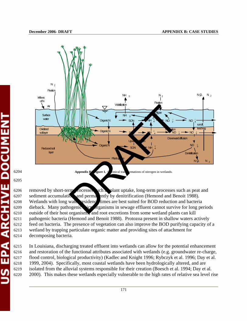
December 2006- DRAFT APPENDIX B: CASE STUDIES
171
Air
Surface water
Oxidizedsoil layer
N
NH
2
3
NO 3
NH 3
Fixation
Organic N
Organic N
Organic N
SON
SON NH 4+
NH 4+
Reduced soillayer
SON NH 4+
Plant uptake
NO 3
NO 3
2N O,2N
2N
2N
2N O,
-
-
NO 2-
NO 2-
Algae
Organic N
Volatilization
Upward diffusion
Denitrification
Downward diffusion
Nitrificationrunoff,leaching
Fixation
Inflows of N
-
Appendix B2 Figure 1. Chemical transformations of nitrogen in wetlands. 6204
6205
removed by short-term processes such as plant uptake, long-term processes such as peat and 6206 sediment accumulation, and permanently by denitrification (Hemond and Benoit 1988). 6207 Wetlands with long water residence times are best suited for BOD reduction and bacteria 6208 dieback. Many pathogenic microorganisms in sewage effluent cannot survive for long periods 6209 outside of their host organisms, and root excretions from some wetland plants can kill 6210 pathogenic bacteria (Hemond and Benoit 1988). Protozoa present in shallow waters actively 6211 feed on bacteria. The presence of vegetation can also improve the BOD purifying capacity of a 6212 wetland by trapping particulate organic matter and providing sites of attachment for 6213 decomposing bacteria. 6214
In Louisiana, discharging treated effluent into wetlands can allow for the potential enhancement 6215 and restoration of the functional attributes associated with wetlands (e.g. groundwater re-charge, 6216 flood control, biological productivity) (Kadlec and Knight 1996; Rybczyk et al. 1996; Day et al. 6217 1999, 2004). Specifically, most coastal wetlands have been hydrologically altered, and are 6218 isolated from the alluvial systems responsible for their creation (Boesch et al. 1994; Day et al. 6219 2000). This makes these wetlands especially vulnerable to the high rates of relative sea level rise 6220
DRAFT
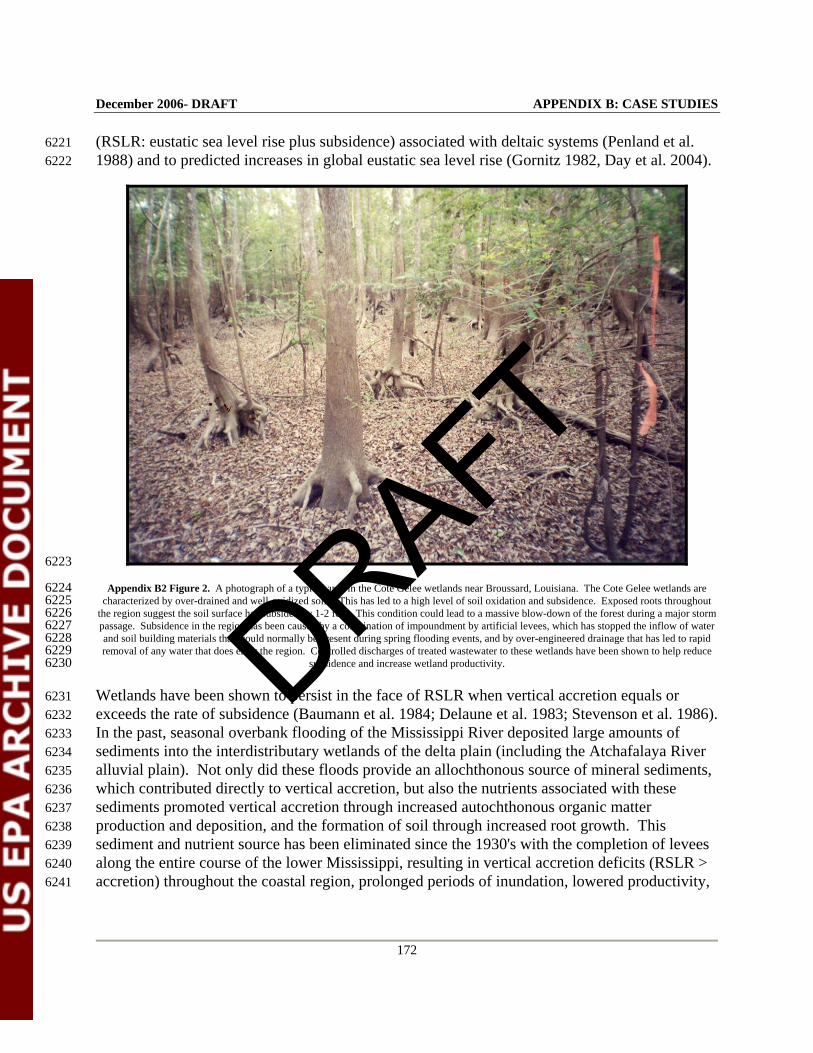
December 2006- DRAFT APPENDIX B: CASE STUDIES
172
(RSLR: eustatic sea level rise plus subsidence) associated with deltaic systems (Penland et al. 6221 1988) and to predicted increases in global eustatic sea level rise (Gornitz 1982, Day et al. 2004). 6222
6223
Appendix B2 Figure 2. A photograph of a typical area in the Cote Gelee wetlands near Broussard, Louisiana. The Cote Gelee wetlands are 6224 characterized by over-drained and well-oxidized soils. This has led to a high level of soil oxidation and subsidence. Exposed roots throughout 6225
the region suggest the soil surface has subsided by 1-2 feet. This condition could lead to a massive blow-down of the forest during a major storm 6226 passage. Subsidence in the region has been caused by a combination of impoundment by artificial levees, which has stopped the inflow of water 6227 and soil building materials that would normally be present during spring flooding events, and by over-engineered drainage that has led to rapid 6228 removal of any water that does enter the region. Controlled discharges of treated wastewater to these wetlands have been shown to help reduce 6229
subsidence and increase wetland productivity. 6230
Wetlands have been shown to persist in the face of RSLR when vertical accretion equals or 6231 exceeds the rate of subsidence (Baumann et al. 1984; Delaune et al. 1983; Stevenson et al. 1986). 6232 In the past, seasonal overbank flooding of the Mississippi River deposited large amounts of 6233 sediments into the interdistributary wetlands of the delta plain (including the Atchafalaya River 6234 alluvial plain). Not only did these floods provide an allochthonous source of mineral sediments, 6235 which contributed directly to vertical accretion, but also the nutrients associated with these 6236 sediments promoted vertical accretion through increased autochthonous organic matter 6237 production and deposition, and the formation of soil through increased root growth. This 6238 sediment and nutrient source has been eliminated since the 1930's with the completion of levees 6239 along the entire course of the lower Mississippi, resulting in vertical accretion deficits (RSLR > 6240 accretion) throughout the coastal region, prolonged periods of inundation, lowered productivity, 6241
DRAFT

December 2006- DRAFT APPENDIX B: CASE STUDIES
173
marsh loss, and a lack of regeneration in forested wetlands. Primarily because of these impacts, 6242 there has been a massive loss of coastal wetlands (Day, et al. 2004; Day, et al. 2000). 6243
Contributing further to the problem of vertical accretion deficits, many wetlands in the 6244 Atchafalaya River alluvial plain have been hydrologically isolated from surrounding marshes, 6245 swamps and bayous due to an exponential increase in the construction of canals and spoil banks 6246 during the past century (Turner and Cordes 1987). In addition to impeding drainage and, in 6247 many cases, physically impounding wetlands, these spoil banks also prevent the overland flow of 6248 sediments and nutrients into cypress/tupelo forests, creating essentially ombrotrophic systems 6249 from what were naturally eutrophic or mesotrophic. 6250
The total acreage of swamp forest in Louisiana has been drastically decreased by 50% from 1956 6251 to 1990 (Barras et al. 1994). Furthermore, it has been predicted that increased rates of eustatic 6252 sea level rise and associated increase in salinity could eliminate most of the remaining forested 6253 wetlands (Delaune et al. 1987). In the wetland forests of southeastern Louisiana, Conner and 6254 Day (1988) estimated vertical accretion deficits ranging from 2.5 to 10.8 mm/yr, which leads 6255 directly to increased flooding duration, frequency and intensity. Productivity decreases observed 6256 in these wetlands may be attributed to either the direct physio-chemical effects of flooding (i.e. 6257 anoxia or toxicity due to the reduced species of S and Fe), flood related nutrient limitations (i.e. 6258 denitrification or the inhibition of mineralization), nutrient limitations due to a reduction in 6259 allocthonous nutrient supplies, lack of regeneration, or most likely, a combination of these 6260 factors (Mitsch and Gosselink 2000). For those wetlands which are not threatened by rising sea 6261 level, there is a high rate of soil subsidence caused by over drainage. 6262
Recent efforts to restore and enhance wetlands in the subsiding delta region have focused on 6263 attempts to decrease vertical accretion deficits by either physically adding sediments to wetlands 6264 or by installing sediment trapping mechanisms (i.e. sediment fences), thus increasing elevation 6265 and relieving the physio-chemical flooding stress (Boesch et al 1994; Day et al. 1992, 1999, 6266 2004). Breaux and Day (1994) proposed an alternate restoration strategy by hypothesizing that 6267 adding nutrient rich secondarily treated wastewater to hydrologically isolated and subsiding 6268 wetlands could promote vertical accretion through increased organic matter production and 6269 deposition. Their work, along with other studies, has shown that treated wastewater does 6270 stimulate productivity and accretion in wetlands (Odum et al. 1975; Mudroch and Copobianco 6271 1979; Bayley et al. 1995; Turner et al. 1976; Knight 1992; Craft and Richardson 1993; Hesse et 6272 al. 1998; Rybczyk 1997). Rybczyk et al. (2002) reported that effluent application at Thibodaux, 6273 Louisiana, increased accretion rates by a factor of three. 6274
The introduction of treated municipal wastewater into the highly perturbed forested wetlands of 6275 Louisiana may be an important step towards their ecological restoration. The nutrient 6276 component of wastewater effluent increases tree productivity (Hesse et al. 1998; Rybczyk 1996), 6277 which helps offset regional subsidence by increasing organic matter deposition enhanced organic 6278 soil formation) on the wetland surface. Increasing productivity results in greater root production 6279 which leads to organic soil formation. This action can enhance the accretion necessary to offset 6280
DRAFT

December 2006- DRAFT APPENDIX B: CASE STUDIES
174
the subsidence that contributes to wetland loss (Day, et al. 2004). The freshwater component of 6281 effluent provides a buffer for saltwater intrusion events, especially during periods of drought, 6282 which are predicted to increase in frequency in the future due to global climate change (Day, et 6283 al. 2004). These ecological benefits to wetlands are in addition to providing candidate 6284 municipalities with an economical means to meet more stringent water quality standards in the 6285 future. 6286 6287 The purpose of the Louisiana Water Control Law is to protect or enhance the quality of public 6288 water, including wetlands. Three components of the water quality standards adopted by 6289 Louisiana and approved by the EPA are; 1) beneficial water uses such as propagation of fish and 6290 wildlife, 2) criteria to protect these beneficial uses, and 3) an antidegradation policy which limits 6291 the lowering of water quality. Municipalities contemplating a discharge to wetlands are required 6292 to conduct a use attainability analysis (UAA) that is submitted to the Louisiana Department of 6293 Environmental Quality as part of the permit process. A UAA describes background ecological 6294 conditions of the candidate site (hydrology, soil and water chemistry, vegetation, animal 6295 populations), analyzes the feasibility of wetland treatment, and provides preliminary engineering 6296 design and cost analyses. A number of UAA studies have been carried out to examine the effect 6297 of wetlands on effluent water quality, sediment accretion, wetland productivity, and economic 6298 savings (e.g. Day, et al. 1994; Day, et al. 1997a; Day, et al. 1997b). Various aspects of these 6299 studies have been published in the scientific literature (Breaux and Day, 1994; Blahnik and Day, 6300 2000; Rybczyk, et al. 1996) and in a number of theses and dissertations (Breaux, 1992; Hesse, 6301 1994; Westphal, 2000). The following sections briefly describe some of the beneficial 6302 environmental effects of treated wastewater discharged to wetlands as documented in case 6303 studies conducted by researchers in Louisiana in cooperation with the Louisiana Department of 6304 Environmental Quality, the US EPA, the US Army Corps of Engineers, the Louisiana Sea Grant 6305 Program, the National Coastal Resources Research and Development Institute, the Louisiana 6306 Department of Natural Resources. Local governments that have participated in these studies 6307 include the towns of Thibodaux, Breaux Bridge, Amelia, Hammond, Mandeville, St. Martinville, 6308 and Broussard; and the parishes of St. Bernard, St. Charles, and Jefferson. Cost benefit and 6309 energy savings are not discussed here, but can be found in the UAA studies and some of the 6310 references listed with this review. 6311 6312 Effects on Effluent Quality – N and P Reductions 6313 6314 Loading rates and percent nutrient reductions for several municipal discharges to wetlands sites 6315 in Louisiana are listed in Table 1 below. Zhang et al. (2000) described the effects of wastewater 6316 effluent on wetland water quality in the Point au Chene wetland for the City of Thibodaux, 6317 Louisiana. In general, the researchers found that within the immediate 231 ha zone of discharge, 6318 N and P concentrations were reduced 100% and 66% respectively from effluent inflow to 6319 outflow. In a related review, Rybczyk et al. (1998) concluded that the effluent processing could 6320 be attributed to: 6321 6322
DRAFT
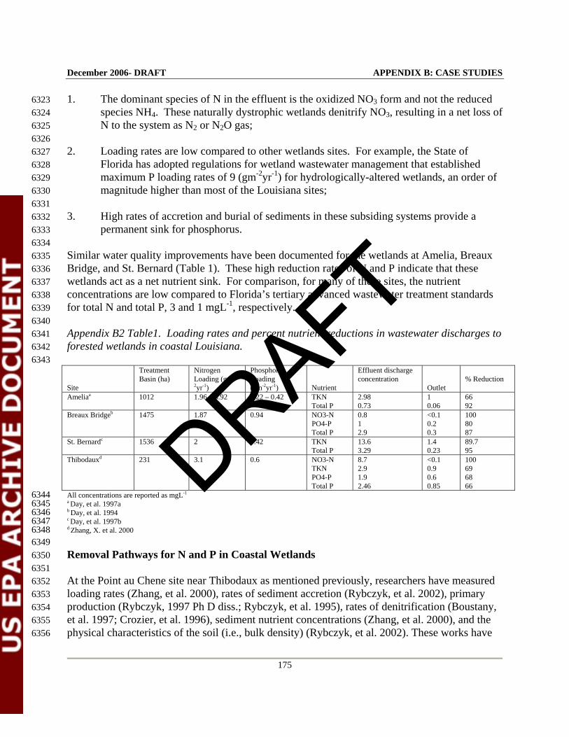
December 2006- DRAFT APPENDIX B: CASE STUDIES
175
1. The dominant species of N in the effluent is the oxidized NO3 form and not the reduced 6323 species NH4. These naturally dystrophic wetlands denitrify NO3, resulting in a net loss of 6324 N to the system as N2 or N2O gas; 6325
6326 2. Loading rates are low compared to other wetlands sites. For example, the State of 6327
Florida has adopted regulations for wetland wastewater management that established 6328 maximum P loading rates of 9 (gm-2yr-1) for hydrologically-altered wetlands, an order of 6329 magnitude higher than most of the Louisiana sites; 6330
6331 3. High rates of accretion and burial of sediments in these subsiding systems provide a 6332
permanent sink for phosphorus. 6333 6334
Similar water quality improvements have been documented for the wetlands at Amelia, Breaux 6335 Bridge, and St. Bernard (Table 1). These high reduction rates of N and P indicate that these 6336 wetlands act as a net nutrient sink. For comparison, for many of these sites, the nutrient 6337 concentrations are low compared to Florida’s tertiary advanced wastewater treatment standards 6338 for total N and total P, 3 and 1 mgL-1, respectively. 6339 6340 Appendix B2 Table1. Loading rates and percent nutrient reductions in wastewater discharges to 6341 forested wetlands in coastal Louisiana. 6342 6343 Site
Treatment Basin (ha)
Nitrogen Loading (gm-
2yr-1)
Phosphorus Loading (gm-2yr-1)
Nutrient
Effluent discharge concentration
Outlet
% Reduction
Ameliaa 1012 1.96 – 3.92 0.22 – 0.42 TKN Total P
2.98 0.73
1 0.06
66 92
Breaux Bridgeb 1475 1.87 0.94 NO3-N PO4-P Total P
0.8 1 2.9
<0.1 0.2 0.3
100 80 87
St. Bernardc 1536 2 0.42 TKN Total P
13.6 3.29
1.4 0.23
89.7 95
Thibodauxd 231 3.1 0.6 NO3-N TKN PO4-P Total P
8.7 2.9 1.9 2.46
<0.1 0.9 0.6 0.85
100 69 68 66
All concentrations are reported as mgL-1 6344 a Day, et al. 1997a 6345 b Day, et al. 1994 6346 c Day, et al. 1997b 6347 d Zhang, X. et al. 2000 6348 6349 Removal Pathways for N and P in Coastal Wetlands 6350 6351 At the Point au Chene site near Thibodaux as mentioned previously, researchers have measured 6352 loading rates (Zhang, et al. 2000), rates of sediment accretion (Rybczyk, et al. 2002), primary 6353 production (Rybczyk, 1997 Ph D diss.; Rybczyk, et al. 1995), rates of denitrification (Boustany, 6354 et al. 1997; Crozier, et al. 1996), sediment nutrient concentrations (Zhang, et al. 2000), and the 6355 physical characteristics of the soil (i.e., bulk density) (Rybczyk, et al. 2002). These works have 6356
DRAFT

December 2006- DRAFT APPENDIX B: CASE STUDIES
176
allowed for the quantification of the loss pathways of N and P at the 231 ha site and are shown in 6357 Table 2 below. 6358 6359 Appendix B2 Table 2. Estimated fate of effluent N and P entering the Point au Chene/Thibodaux 6360 site. 6361 6362 Total N
(g m-2yr-1) Total P (g m-2yr-1)
A. Storage in sediments (burial). Calculated as the mean rate of accretion in the immediate impact zone (1.14 cm/yr) x mean conc. of total N (4.95 mg/g) or P (1.25 mg/g) in the upper 4 cm of soil x mean bulk density (0.13 g/cm3) of soil in the upper 4 cm.
7.3
1.8
B. Storage in woody vegetation. Calculated as mean annual increase in bole wood (285 g m-2yr-1) x mean conc. of N (0.39%) and P (0.11%) in wood.a
1.1
0.03
C. Potential denitrification rates 36 - D. Total 44.6 1.83 E. Loading rate
Calculated as the mean hydraulic loading rate of 6.3 x 10⁶ L-1 day x mean N and P effluent concentrations of 12.6 and 2.46 mg L-1 respectively x basin area (231 ha)
12.5
2.4
All values used to calculate removal and loading rates were derived from data collected at the Thibodaux sites except for estimate of woody tissue 6363 N and P. 6364 a Concentrations of N and P in woody tissue were not measured at the Thibodaux site. Concentrations used here are means from bottomland 6365 hardwood swamps as reported by Johnston, 1991. 6366 6367 Increased Sediment Accretion 6368 6369 As indicated earlier in this review, if coastal wetlands do not accrete vertically at a rate equal to 6370 the RSLR (RSLR: eustatic sea level rise plus subsidence) they can become stressed and can 6371 ultimately disappear (Day, et al. 2004). In coastal regions, especially deltas, naturally high rates 6372 of subsidence can exceed rates of eustatic sea level rise by an order of magnitude (Penland, 6373 1988; Emery and Aubrey, 1991). Accretion deficits (sediment accretion < RSLR) in many 6374 coastal systems are not only the result of high rates of RSLR, but also hydrologic alterations 6375 such as dams, dikes and levees that restrict the natural movement of nutrients and suspended 6376 sediments into wetlands (Day, et al. 2004). In systems affected by high rates of RSLR, 6377 hydrologic alterations, or both, treated effluents can serve as a wetland restoration or 6378 enhancement tool, and can stimulate biomass production and enhance sediment accretion rates 6379 (Rybczyk, et al. 2002; Reddy et al. 1993). Recently, Rybczyk et al. 2002 reported on the effects 6380 of nutrient-rich secondarily treated effluent into the subsiding, forested wetlands at Thibodaux 6381 and found that the effluent promoted vertical accretion through increased organic matter 6382 production and subsequent deposition and allowed accretion to keep pace with rates of RSLR 6383 that approached 1.23 cm yr-1 in comparison to background sediment rates averaging only 0.44 ± 6384 0.04 cm yr-1. 6385 6386 Feldspar horizon marker techniques have been utilized to estimate accretion rate in sites 6387 receiving treated effluent and in adjacent control sites, both before and after wastewater 6388 applications (Cahoon, 1989). No significant difference between pre-effluent and control 6389
DRAFT
December 2006- DRAFT APPENDIX B: CASE STUDIES
177
accretion rates was detected, and after wastewater application began, accretion rates in the 6390 application site (1.1 cm yr-1 ) were significantly higher than accretion rates measured at the 6391 control (0.14 cm yr-1). Analysis of the sediment accretion rates (accretion rate x % organic or % 6392 mineral matter) indicated that only the rates of organic matter accumulation increased 6393 significantly after effluent application began, which the authors attributed to effluent-stimulated 6394 organic matter accretion. It could also be hypothesized that nutrient enrichment would stimulate 6395 the decomposition of organic matter, thus negating any increase in accretion due to increased 6396 organic matter accumulation, and to test this hypothesis in the same study researchers measured 6397 decomposition rates and litter nutrient dynamics in the wetland application site and in the 6398 adjacent control site, both before and after applications began. A before-and-after-control-6399 impact (BACI) statistical analysis revealed that neither leaf-litter decomposition rates nor initial 6400 leaf-litter N and P concentrations were affected by wastewater effluent; similar analysis revealed 6401 that final N and P leaf-litter concentrations did increase in the effluent application site relative to 6402 the control after effluent was applied. Wetland elevation/sediments dynamics modeling 6403 (Rybczyk, 1998) revealed that changes in wetland elevation were much more responsive to 6404 changes in primary production than to changes in rates of decomposition and suggests that 6405 increased organic matter production and accretion would offset any increases in rates of 6406 decomposition. The model also indicated that nutrient addition alone was not sufficient to lead 6407 to long term restoration of the forested wetland and that some mineral sediment input was 6408 necessary. 6409 6410 Carbon Sequestration 6411 6412 Data to date on accretion and burial indicate that addition of nutrient-rich effluents to subsiding 6413 wetlands can substantially enhance the rate of carbon burial and sequestration. For example, in 6414 Thibodaux (Point au Chene) swamp accretion rates increased and calculated carbon burial rates 6415 increased by almost a factor of three. 6416 6417 Increased Productivity 6418 6419 While stimulating vegetative productivity with treated effluent could lead to eutrophication in 6420 some aquatic systems, many wetlands, including those in coastal Louisiana, are naturally 6421 dystrophic (Day, et al. 2004). The long-term effects of effluent discharge to coastal systems can 6422 be assessed by evaluating data from a forested wetland in Breaux Bridge, Louisiana, that has 6423 been receiving wastewater for over 50 years (Blahnik and Day, 2000; Breaux and Day, 1994). 6424 Dendrological studies (Hesse, et al. 1998; Hesse 1994) to determine long-term effects on 6425 aboveground productivity. Stem wood growth rates from 1920 to 1992 was measured at the 6426 application site and control site (no wastewater application) and an annual diameter increment 6427 ratio calculated by comparing stem wood growth from each site. Before wastewater application 6428 began (according to records between 1948 and 1953) there was significantly higher growth in the 6429 control site than at the application site. However, after the onset of effluent application, there 6430 was increased growth in the application site, resulting in statistically significant higher annual 6431
DRAFT

December 2006- DRAFT APPENDIX B: CASE STUDIES
178
diameter increment ratios. Short term studies (during 1994 -1995) at the same site had similar 6432 findings, i.e. where total production was significantly higher in a new application site as 6433 compared to the old application site. This difference was attributed to increases in stem wood 6434 biomass in the new treatment site and not leaf production. Similar results were reported for the 6435 City of Amelia, Ramos wetland site (Day, et al., 1997a; Westphal, 2000) where a year-long 6436 study on primary productivity indicated enhanced litterfall in the application sites. 6437 6438 Studies have also shown that the production of herbaceous vegetation in coastal wetlands, both 6439 emergent and floating, is also stimulated by wastewater effluent, and may contribute to sediment 6440 accretion to a greater extent than does woody vegetation (Rybczyk, 1997). Percent cover is also 6441 influenced by the seasons and warm temperatures, and can affect the type of cover (i.e., 6442 deciduous canopy to floating aquatic vegetation). 6443 6444 Regulatory and policy considerations 6445 6446 In Louisiana, scientists, state and federal regulators, and dischargers have worked closely over 6447 the past 15 years to develop an approach to meet water quality goals in terms of discharges to 6448 subsiding wetlands. The process has allowed scientists and regulators to gain a great amount of 6449 information about characterizing these coastal wetlands and developing the appropriate criteria 6450 within the state’s water quality standards to protect, monitor and assess them. In these cases, a 6451 preliminary or feasibility study (two to four months) is conducted to determine whether a 6452 discharger is a candidate for this process (to discharge to a wetland site). After the feasibility 6453 study and in consultation with state and federal regulators, if it is decided to continue with the 6454 process a year-long UAA is initiated in which: 1) the background ecological conditions of the 6455 site are described (hydrology, wetland classification, soil and water chemistry, vegetation, 6456 animal populations, and toxic materials) and analyzed; and 2) the potential impacts (along with 6457 loading rates) of the wastewater discharge are evaluated. In addition to any ecological benefits, 6458 a cost-benefit analysis is also conducted. At the conclusion of the UAA, the study results are 6459 again reviewed by standards and permit staff in the Louisiana Department of Environmental 6460 Quality. If appropriate, the beneficial Clean Water Act uses and protective criteria are 6461 recommended by the Louisiana Department of Environmental Quality for adoption into the 6462 water quality standards. The UAA then forms part of the permit application process. The permit 6463 designates effluent limits for the discharge (generally at secondary treatment levels in terms of 6464 BOD and TSS parameters) and the design loading rate (and distribution) ensures high nutrient 6465 assimilation. Disinfection is required so pathogens are not discharged to the wetlands and there 6466 should be no significant industrial use of the wastewater treatment system. After the permit is 6467 issued, the discharger constructs the project, starts discharge and initiates monitoring. 6468 Monitoring is required for the life of the permit and with annual monitoring reports. 6469 6470 Wetland monitoring requirements to assess against the recommended wetland criteria are 6471 incorporated as a part of the permit. Monitoring requirements therefore may include, but are not 6472 limited to, water stage monitoring, analysis of sediment, wetland faunal assemblages for fish and 6473
DRAFT
December 2006- DRAFT APPENDIX B: CASE STUDIES
179
macroinvertebrates, and above-ground wetland productivity (tree, grass, and/or marsh grass 6474 productivity). It should be noted that recent review of the past ten years work in the wetland 6475 UAAs indicates that faunal (benthic and nekton communities) show no clear difference between 6476 areas of effluent application and control areas and may not be appropriate as criteria in many 6477 Louisiana wetlands. Examples of wetland criteria that have been promulgated for wetland sites 6478 in Louisiana’s water quality standards (Louisiana Environmental Regulatory Code, Title 33, Part 6479 IX, Subpart 1, Chapter 11, §1123, Table 3) include faunal and/or vegetative species and/or 6480 abundance, naturally occurring litter fall or stem growth, and the dominance index or stem 6481 density of bald cypress. All other general and numerical criteria not specifically revised in the 6482 standards regulations would generally apply (i.e. narratives, numerical criteria for toxics, etc.). 6483
DRAFT
December 2006- DRAFT APPENDIX B: CASE STUDIES
180
References 6484
Barras, J. A., P. E. Bourgeois, and L. R. Handley. 1994. Land Loss in Coastal Louisiana: 1956-6485 90. National Biological Survey, National Wetlands Research Center. Open File Report 6486 94-01. 4pp. 10 color plates. 6487
Baumann, R. H., J. W. Day, and C. Miller. 1984. Mississippi. deltaic wetland survival; 6488 sedimentation versus coastal submergence. Science. 224: 1093-1095. 6489
Bayley, P. B. 1995. “Understanding large river-floodplain ecosystems.” Bioscience 45 (3): 6490 153-158. 6491
Blahnik, T. and J. Day. 2000. The effects of varied hydraulic and nutrient loading rates on water 6492 quality and hydrologic distributions in a natural forested wetland. Wetlands. 20: 48-61. 6493
Boesch, D. F., M. N. Josselyn, A. J. Mehta, J. T. Morris, W. K. Nuttle, C. A. Simenstad, and D. 6494 J. Smith. 1994. Scientific assessment of coastal wetland loss, restoration and 6495 management in Louisiana. Journal of Coastal Research, Special Issue No. 20. 6496
Boustany, R. G., C. R. Crozier, J. M. Rybczyk, and R. R. Twilley. 1997. Denitrification in a 6497 south Louisiana wetland forest receiving treated sewage effluent. Wetland Ecology and 6498 Management 4: 273-283. 6499
Boyt, F.L. 1976. A mixed hardwood swamp as an alternative to tertiary wastewater treatment. 6500 M.S. thesis, University of Florida, Gainesville, FL. 6501
Boyt, F. L., S. E. Bayley, and J. Zoltek, JR. 1977. Removal of nutrients from treated municipal 6502 wastewater by wetland vegetation. J. Water Pollution Control Federation 49:789-799. 6503
Breaux, A. M. 1992. The use of hydrologically altered wetlands to treat wastewater in coastal 6504 Louisiana. Ph D dissertation, Louisiana State University. 6505
Breaux, A. M. and J. W. Day, Jr. 1994. Policy Considerations for Wetland Wastewater 6506 Treatment in the Coastal Zone: A Case Study for Louisiana. Coastal Management. 6507 22:285-307. 6508
Cahoon, D. R. and R. E. Turner. 1989. Accretion and canal impacts in a rapidly subsiding 6509 wetland II. Feldspar marker horizon technique. Estuaries 12(4): 260-268. 6510
Conner, W. H. and J. W. Day, Jr. 1988. The impact of rising water levels on tree growth in 6511 Louisiana. Pages 219-224 in Hook, D. D. et al. (eds.), the Ecology and Management of 6512 Wetlands, Vol. 2: Management, Use and Value of Wetlands. Croom Helm Ltd 6513 Publishers, England. 6514
DRAFT
December 2006- DRAFT APPENDIX B: CASE STUDIES
181
Conner, W.H., J. W. Day, Jr, and J. D. Bergeron. 1989. A use attainability analysis of wetlands 6515 for receiving treated municipal and small industry wastewater: a feasibility study using 6516 baseline data from Thibodaux, LA. Center for Wetland Resources, Louisiana State 6517 University, Baton Rouge, LA. 78 p. 6518
Craft, C. B. and C. J. Richardson. 1993. Peat accretions and phosphorus accumulation along a 6519 eutrophication gradient in the northern Everglades. Biogeochemistry 22:133-156. 6520
Crozier, C. R., J. M. Rybczyk, and W. H. Patrick, Jr. 1996. Spatial gradients of dissolved nitrate 6521 and nitrous oxide in a wetland forest receiving treated sewage effluent. In: Flynn, K. ed. 6522 Proc. of the Southern Forested Wetlands Ecology and Management Conference. South 6523 Carolina: Clemson University. Pp. 78-82. 6524
Day, J. W., A. M. Breaux, I. D. Hesse and J. M. Rybczyk. 1992. Wetland wastewater treatment 6525 in the Louisiana coastal zone. Barataria-Terrebone National Estuary Program: Data 6526 Inventory Workshop Proceedings: Pages 221-238. 6527
Day, J. W., A. M. Breaux, S. Feagley, P. Kemp, and C. Courville. 1994. A use attainability 6528 analysis for long-term wastewater discharge on the Cypriere Perdue Forested Wetland at 6529 Breaux Bridge, Louisiana. Coastal Ecology Institute, Louisiana State University. 6530
Day, J. W., J. M. Rybczyk, R. I. Pratt, A. Westphal, T. Blahnick, G. Garson, and G.P. Kemp. 6531 1997a. A Use Attainability Analysis of long-term wastewater discharge on the Ramos 6532 forested wetland at Amelia, LA. Coastal Ecology Institute Report, prepared for St. Mary 6533 Parish Water and Sewer Commission #1, Town of Amelia, Louisiana. 6534
Day, J. W., Rybczyk, J. M., R. Pratt, M. Sutula, A. Westphal, T. Blahnik, P. Delgado, P. Kemp, 6535 A. J. Englande, C. Y. Hu, G. Jin, H. W. Jeng. 1997b. A Use Attainability Analysis for 6536 longterm wastewater discharge to the Poydras-Verret Wetland in St. Bernard Parish, 6537 Louisiana. Coastal Ecology Institute, Louisiana State University. 6538
Day, J., Jr., J. Rybczyk, W. Conner, P. Delgado, S. Feagley, I. Hessse, R. Pratt, A. Westphal, and 6539 X. Zhang. 1998. The use of swamp forests near Thibodaux, Louisiana for application of 6540 treated municipal wastewater: Monitoring the effects of the discharge 1992-1997. 6541 Coastal Ecology Institute, Louisiana State University, Baton Rouge, Louisiana. 6542
Day, J.W., Jr., J.M. Rybczyk, L. Cardoch, W. Conner, P. Delgado-Sanchez, R. Pratt, A. 6543 Westphal. 1999. A review of recent studies of the ecological and economical aspects of 6544 the application of secondarily treated municipal effluent to wetlands in Southern 6545 Louisiana. pp. 155-166. In: L. Rozas, J. Nyman, C. Proffitt, N. Rabalais, and R. Turner 6546 (eds.) Recent Research in Coastal Louisiana. Louisiana Sea Grant College Program, 6547 Louisiana State University, Baton Rouge. 6548
Day, J., G. Shaffer, L. Britsch, D. Reed, S. Hawes, and D. Cahoon. 2000a. Pattern and process of 6549
DRAFT
December 2006- DRAFT APPENDIX B: CASE STUDIES
182
land loss in the Mississippi delta: A spatial and temporal analysis of wetland habitat 6550 change. Estuaries. 23: 425-438. 6551
6552 Day, J. W., Jae-Young Ko, J. Rybczyk, D. Sabins, R. Bean, G. Berthelot, C. Brantley, L. 6553
Cardoch, W. Conner, J.N. Day, A.J. Englande, S. Feagley, E. Hyfield, R. Lane, J. 6554 Lindsey, J. Mistich, E. Reyes, and R. Twilley. 2004. The use of wetlands in the 6555 Mississippi Delta for wastewater assimilation: a review. Ocean and Coastal 6556 Management 47: 671-691. 6557
6558 DeLaune, R.D., R.H. Baumann, and J.G. Gosselink. 1983. Relationships among vertical 6559
accretion, coastal submergence, and erosion in a Louisiana Gulf Coast marsh. Journal of 6560 Sedimentary Petrology. 53(1):0147-0157. 6561
DeLaune, R. D., C. J. Smith, W. H. Partick, and H. H. Roberts. 1987. Rejuvenated marsh and 6562 bay-bottom accretion on rapidly subsiding coastal plain of U.S. gulf coast: a second-6563 order effect of the emerging Atchafalaya delta. Estuarine, Coastal and Shelf Science. 6564 25:381-389. 6565
Emery, K. O. and D. G. Aubrey. 1991. Sea levels, land levels and tide gauges. New York: 6566 Springer. 6567
Ewel, K. C. and S. E. Bayley. 1978. Cypress strand receiving sewage at Waldo. Pages 750-801 6568 in H.T. Odum and K.C. Ewel, Principal Investigators. Cypress wetlands for water 6569 management, recycling, and conservation. Fourth Annual Report to National Science 6570 Foundation. 6571
Faulkner, S. P. and C. J. Richardson. 1989. Physical and chemical characteristics of freshwater 6572 wetland soils. Pages 41-72 in D.A. Hammer, ed., Constructed Wetlands for Wastewater 6573 Treatment. Lewis Publishers, Michigan. 6574
Gornitz, V., S. Lebedeff, and J. Hansen. 1982. Global sea level trend in the past century. 6575 Science 215: 1611-4. 6576
Hemond, H. F. and J. Benoit. 1988. Cumulative impacts on water quality functions of wetlands. 6577 Environmental Management 12:639-653. 6578
Hesse, I. D., J. Day. 1994. Dendroecological determination of municipal wastewater effects on 6579 Taxodium distichum (L.) rich productivity in a Louisiana swamp. M.S. Thesis, Louisiana 6580 State University. 6581
Hesse, I. D, J. Day, and T. Doyle. 1998. Long-term growth enhancement of Bald cypress 6582 (Taxodium distichum) from municipal wastewater application. Environmental 6583 Management. 22:119-127. 6584
DRAFT
December 2006- DRAFT APPENDIX B: CASE STUDIES
183
Johnston, C. A. 1991. Sediment and nutrient retention by freshwater wetlands: effects on 6585 surface water quality. Critical Reviews in Environmental Control 21: 491-565. 6586
Kadlec, R. H. and H. Alvord, Jr. 1989. Mechanisms of water quality improvement in wetland 6587 treatment systems. Pages 489-498 in D.W. Fisk, ed., Wetlands: Concerns and Successes. 6588 Proceedings sponsored by American Water Resources Association, September 17-22, 6589 1989, Tampa, Florida. 6590
Kadlec, R. H., R. L. Knight. 1996. Treatment Wetlands. Boca Raton. Lewis Publishers. 6591
Kemp, G. P., W. H. Conner, and J. W. Day, Jr. 1985. Effects of flooding on decomposition and 6592 nutrient cycling in a Louisiana swamp forest. Wetlands 5: 35-51. 6593
Khalid, R.A., R.P. Gambrell, W.H. Patrick, Jr. 1981a. An overview of the utilization of 6594 wetlands for wastewater organic carbon removal. Pages 405-423 in Progress in Wetlands 6595 Utilization and Management. Proceedings of a Symposium: 9-12 June 1981. Orlando, 6596 Florida. Sponsored by: Coordinating Council on the Restoration of the Kissimmee River 6597 Valley and Taylor Creek Nubbin Slough Basin. 6598
Khalid, R.A., I.C.R. Holford, M.N. Mixon, and W.H. Patrick. 1981b. Nitrogen and phosphorus 6599 reactions in overland flow of wastewater. U.S. Environmental Protection Agency, EPA-6600 600/S2-81-150. 6601
Kitchens, W. F., Jr., J. M. Dean, L. H. Stevenson, and J. H. Cooper. 1975. The Santee Swamp 6602 as a nutrient sink. Pages 349-366 in F.G. Howell, J.B. Gentry, and M.H. Smith, eds., 6603 Mineral cycling in southeastern ecosystems. Tech. Info. Center, Energy Research and 6604 Development Administration, ERDA Symposium Series 36. Available as CONF-740513 6605 from NTIS, Washington, DC. 6606
Knight, R. L, T. W. McKim, H. R. Kohl. 1987. Performance of a natural wetland treatment 6607 system for wastewater management. Journal of Water Pollution Control Federation, 6608 59(8):746-754. 6609
Knight, R. L. 1992. Natural land treatment with Carolina bays. Water Environment and 6610 Technology 4:13-16. 6611
Kuenzler, E. J. 1987. Impacts of sewage effluent on tree survival, water quality and nutrient 6612 removal in coastal plain swamps. Report No. 235 of the Water Resources Research 6613 Institute of the University of North Carolina, Chapel Hill, NC. 91 p. 6614
6615 Lemlich, S.K. and K.C. Ewel. 1984. Effects of wastewater disposal on growth rates of cypress 6616
trees. J.Environ.Qual., 13(4):602-604. 6617
DRAFT

December 2006- DRAFT APPENDIX B: CASE STUDIES
184
Mitsch, W. J. and J. G. Gosselink. 2000. The value of wetlands: importance of scale and 6618 landscape setting. Ecological Economics 35 (200) 25-33. 6619
Murdroch, J. and J. A. Capobianco. 1979. Effects of Treated Effluent on Natural Marsh. J. of 6620 Water Pollution Control Federation 51: 2243-2256. 6621
Nessel, J. K. 1978. Distribution and dynamics of organic matter and phosphorus in a sewage 6622 enriched cypress swamp. M.S. thesis, University of Florida, Gainesville, FL. 6623
Nessel, J. K. and S. E. Bayley. 1984. Distribution and dynamics of organic matter and 6624 phosphorus in a sewage-enriched cypress swamp. Pages 262-278 in K.C. Ewel and H.T. 6625 Odum, eds. Cypress Swamps, University Presses of Florida, Gainesville, FL. 6626
Nichols, D. S. 1983. Capacity of natural wetlands to remove nutrients from wastewater. 6627 Journal of Water Pollution Control Federation 55(5): 495-505. 6628
Odum, H. T. 1975. Energy quality and carrying capacity of the earth. Tropical Ecology. 16:1-8. 6629
Odum, H. T. 1978. Value of wetlands as domestic ecosystems. Pages 910-930 in H.T. Odum 6630 and K.C. Ewel, eds., Cypress Wetlands for Water Management, Recycling, and 6631 Conservation. Fourth Annual Report to National Science Foundation and the Rockefeller 6632 Foundation. 6633
Patrick, W. H., Jr. 1990. Microbial reactions of nitrogen and phosphorus in wetlands. Pages 6634 52-63 in the Utrecht Plant Ecology News Report, Utrecht, The Netherlands. 6635
Penland, S., K. E. Ramsey, R. A. McBride, J. T. Mestayer, and K. A. Westphal. 1988. Relative 6636 sea level rise and delta plain development in the Terrebonne parish region. Coastal 6637 geology technical report, Baton Rouge, Louisiana: Louisiana Geological Survey. 121 pp. 6638
Reddy, K. R., R. D. DeLaune, W. F. DeBusk, M. S. Koch. 1993. Long-term nutrient 6639 accumulation rates in the everglades. Soil Science Society of America Journal 57: 1147-6640 1155. 6641
Richardson, C. J. and J. A. Davis. 1987. Natural and artificial ecosystems: ecological 6642 opportunities and limitations. Pages 819-854 in K.R. Reddy and W.H. Smith, eds., 6643 Aquatic Plants for Water Treatment and Resource Recovery, Magnolia Publishing, Inc, 6644 Orlando, FL. 6645
Richardson, C. J. and D. S. Nichols. 1985. Ecological analysis of wastewater management 6646 criteria in wetland ecosystems. Pages 351-391 in P.J. Godfrey, E.R. Kaynor, and S. 6647 Pelczarski, eds. Ecological considerations in wetlands treatment of municipal 6648 wastewaters, Van Nostrand Reinhold Company, NY. 6649
DRAFT

December 2006- DRAFT APPENDIX B: CASE STUDIES
185
Rybczyk, J. M., J. W. Day, I. D. Hesse, and P. Delgado-Sanchez. 1995. The impact of 6650 Hurricane Andrew on tree mortality, litterfall, nutrient flux and water quality in a 6651 Louisiana coastal swamp forest. Journal of Coastal Research 21: 340-353. 6652
Rybczyk, J. M., J. W. Day, I. D. Hesse and P. Delgado Sanchez. 1996. An overview of forested 6653 wetland wastewater treatment projects in the Mississippi River delta region. Proceedings 6654 of the Southern Forested Wetlands Ecology and Management Conference. Kathryn Flynn 6655 (Ed.) Clemson University, South Carolina. Pages 78-82. 6656
Rybczyk, J. M. 1997. The use of secondarily treated wastewater effluent for forested wetland 6657 restoration in a subsiding coastal zone. Ph D dissertation. Louisiana State University. 6658
Rybczyk, J. M., J. C. Callaway and J. W. Day, Jr. 1998. A relative elevation model (REM) for a 6659 subsiding coastal forested wetland receiving wastewater effluent. Ecological Modeling 6660 112: 23-44. 6661
Rybczyk, J. M., J. Day, and W. Conner. 2002. The impact of wastewater effluent on accretion 6662 and decomposition in a subsiding forested wetland. Wetlands. 22(1): 18-32. 6663
Shih, S. F. and D. W. Hallett. 1974. Impact of upland marsh on water quality. Internal Report, 6664 Department of Resource Planning, Central and Southern Florida Flood Control District, 6665 West Palm Beach, FL. 6666
Stevenson, J. C., L. G. Ward and M. S. Kearney. 1986. Vertical accretion in marshes with 6667 varying rates of sea level rise, Pages 241-260. In D. Wolf (ed.) Estuarine variability. 6668 Academic Press, New York. 6669
Turner, R.E. et al. 1976. Aspects of Land-Treated Waste Application in Louisiana Wetlands. 6670 In: Proceedings of the National Symposium on Freshwater Wetlands and Sewage 6671 Effluent Disposal. Tilton D.L. editor. Pages 147-167. 6672
Turner, R. and C. Cordes. 1987. Relationship between canal and levee density and coastal land 6673 loss in Louisiana. Biological Report 85(14), U.S. Fish and Wildlife Service, Washington. 6674
Tuschall, J. R., P. L. Brezonik, and K. C. Ewel. 1981. Tertiary treatment of wastewater using 6675 flow-through wetland systems. Proc. 1981 Annual Conference of the American Society 6676 of Civil Engineers, Environmental Division. 6677
U.S. Environmental Protection Agency. 1987. Report on the Use of Wetlands for Municipal 6678 Wastewater Treatment and Disposal. Office of Water, Office of Municipal Pollution 6679 Control. Submitted to: Senator Quentin N. Burdick, Chairman of Committee on 6680 Environmental and Public Works. EPA 430/09-88-005. 6681
DRAFT
December 2006- DRAFT APPENDIX B: CASE STUDIES
186
Wharton, C.H. 1970. The southern river swamp - a multiple use environment. School of 6682 Business Administration, Georgia State University, Atlanta, GA. 6683
Westphal, A. 2000. Effects of municipal effluent on the nutrient dynamics and productivity of a 6684 coastal forested wetland in Louisiana. M. S. thesis, Louisiana State University. 6685
Yarbro, L. A. 1979. Phosphorus cycling in the Creeping Swamp floodplain ecosystem and 6686 exports from the Creeping Swamp watershed. Ph.D. dissertation, University of North 6687 Carolina, Chapel Hill, NC. 231 p. 6688
Yarbro, L.A., E. J. Kuenzler, P.L. Mulholland, and R. P. Sniffen. 1982. The influence of swamp 6689 floodplain on exports of nitrogen and phosphorus from North Carolina coastal plain 6690 watersheds. Pages 225-241 in P.M. McCaffrey, T. Beemer, and S.E. Gatewood, eds. 6691 Proc. of the Symposium, Progress in wetlands utilization and management. Coordinating 6692 Council on Restoration of Kissimee River and Taylor Creek-Nubbin Slough Basin. 6693
Zhang, X., S. Feagley, J. Day, W. Conner, I. Hesse, J. Rybczyk, and W, Hudnall. 2000. A water 6694 chemistry assessment of wastewater remediation in a natural swamp. Journal of 6695 Environmental Quality 29: 1960-1968. 6696
DRAFT