Institute for Research on PovertyDiscussion Paper no. 1041-94

Welfare Effects of Fixed and Percentage-Expressed Child Support Awards

Daniela Del BocaDepartment of Economics

University of Turin

Christopher J. FlinnDepartment of Economics

New York University

August 1994

This research was supported by the Small Grants Program administered by the Institute for Researchon Poverty and the C. N. R. Bilateral Project (Consiglio Nazionale delle Ricerche). We wish to thankUgo Colombino, Pat Brown, Maurice MacDonald, and Daniel Meyer for useful discussions andFrancis Gupta for able research assistance. We are responsible for all opinions expressed as well asfor all errors and omissions.

Abstract

Over the last decade a large number of states have significantly altered their legal statutes

concerning the disposition of divorce cases involving children. In particular, many states have

increasingly employed percentage-expressed orders in which child support obligations in a given

period are determined as a proportion of the contemporaneous income of the noncustodial parent. In

contrast to more traditional systems in which obligations were set in fixed nominal terms at the time of

the divorce settlement and were infrequently (or never) updated, the dynamic system has the

advantages of allowing children (and the custodial parent) an opportunity to share in the general

income gains experienced by the noncustodial parent over the life cycle and of possibly alleviating

some noncompliance problems.

In this paper we conduct a rather extensive theory-based empirical investigation of the effects

of these systems on the income process for divorced fathers and the child support transfer decision.

We estimate a flexible statistical model for the income-generation process for divorced fathers which

encompasses the period both before and after the divorce. We interpret the estimates from this model

to indicate small behavioral effects of the type of order on postdivorce income, but nonrandom

assignment (in terms of the means and variances of predivorce income) into the percentage-expressed-

order state. Our analysis of the effects of the order type on child support transfers is divided into two

parts. In the first, a "reduced form" analysis, we investigate whether or not the divorced father’s

regime—defined as the order type and withholding status—can be considered exogenous vis-á-vis the

transfer decision, and examine the relative effects of the various regimes on the transfer rate. We

further attempt to investigate order-type effects on compliance in the context of a structural model of

the compliance decision. The results of the two analyses are for the most part consistent. Percentage

orders are generally associated with lower compliance rates, though withholding tends to alleviate the

problem. The highest compliance rates are associated with fixed orders coupled with withholding.

Welfare Effects of Fixed and Percentage-Expressed Child Support Awards

1. INTRODUCTION

Child support issues have been actively researched and debated over the past several decades

in response to the substantial decline in the welfare of children living with only one parent.1 Recent

changes in family structure have contributed to an increase in child poverty; nearly all of this increase

can be attributed to the rising proportion of families headed by divorced or never-married mothers.2

The government does not allow noncustodial parents who have been ordered to pay child

support to decide for themselves how much support they will pay; instead, it has authorized the courts

to determine the amount that must be paid. Many custodial parents and children’s advocates have

protested that child support awards are often too low and that courts do not use a preestablished

system to set the amount of payments. Economists and sociologists, therefore, have been searching for

ways to improve the criteria used in setting child support orders.

Research on child support issues can be roughly divided into studies concerned with normative

problems involving the distribution of welfare among divorced parents and their children and studies

assessing the efficiency of various child support policies in achieving certain normative goals. Some

examples of the first type of study include Betson et al. (1992), Garfinkel and Melli (1989), Garfinkel

and Oellerich (1989), Garfinkel et al. (1990), Lazear and Michael (1988), Lerman (1989), Oellerich

and Garfinkel (1983), and Williams (1987). In these analyses, the incomes of the parents before any

child support payments are made are typically taken to be exogenously determined, and policies are

evaluated in terms of their effects on those incomes. Problems of imperfect compliance and

1Good general summaries of the scope of the divorce problem and empirical research on theeffects of custody and child support negotiations and arrangements on the welfare of children anddivorced parents are contained in Weitzman (1985) and Maccoby and Mnookin (1992).

2The proportion of children living with only one parent increased from 14.9 percent in 1970 to 25percent in 1990 (U.S. Bureau of the Census 1991).

2

behavioral responses to child support orders (such as changes in labor supply, job turnover, or

remarriage decisions) are not usually explicitly considered.

The primary focus of the second class of studies is the behavioral response of parents to child

support orders and any income transfers associated with them. For example, Graham and Beller

(1989), Maritato and Robins (1992), and Del Boca (1994) studied the effect of child support income

on the labor supply of custodial mothers; Del Boca and Flinn (1994b) investigated the effect of the

mix of child support and non–child support income of custodial mothers on their expenditures on

"child-specific" goods; and Weiss (1984) studied the effect of divorce on the consumption patterns of

single-parent households. Fewer studies have analyzed the behavioral responses of fathers or both

parents to child support orders; some that have are Garfinkel and Klawitter (1990), Meyer and Bartfeld

(1992), and Del Boca and Flinn (1990), all of which analyze the decision of whether to comply with

child support orders.

The approach taken in the present paper is something of a hybrid, in the sense that the structure

within which the empirical analysis is performed is dictated by theoretical considerations, but the

econometric models utilized are designed for flexibility and ease of interpretation. Only in Section 6

is an explicit behavioral model estimated in order to determine the nature of the effects of order type

on transfers (i.e., child support payments). In all other sections, we have attempted to fit models with

as few restrictions built in as possible, and have concentrated on separating behavioral influences of

order type from spurious relationships induced by systematic selection in the various order regimes.

The plan of the paper is as follows. Section 2 contains an informal description of some of the

behavioral and welfare issues connected with the design of child support orders. In Section 3 we

provide an overview of the data used in the three sections of empirical analysis included here.

(Different subsamples from these data are utilized in the three sections, and the relevant subsample is

described in more detail within each section.) In Section 4 we present the results of the estimation of

3

a "treatment effects" model of order type on the income-generation process. Data on the personal

income of divorced fathers (distinguished by the type of child support order they eventually receive)

both before and after the divorce is used to determine the effects of awards on the mean and variance

of their income processes. Section 5 contains estimates of the relationship between transfers, order

amount, order type, and father’s income in the year following the divorce. We test whether order type

is endogenous in the child support regression function, and generally find evidence that it is not. We

find that order type has large effects on transfers (also loosely interpretable as compliance, given the

regression function specification we use), with fathers with fixed awards and routine withholding

having the highest "compliance rates." Section 6 contains an analysis of the transfer decision within a

behavioral model in which transfers and "compliance" are functions of the mother’s and father’s

incomes and the level of the child support order, as well as preference parameters describing the

weighting of the child’s welfare in the father’s utility function and the cost of noncompliance. We

estimate the structural model for fathers with fixed and percentage-expressed orders separately, to

determine whether fathers under the two regimes have different preferences and/or different costs of

noncompliance. Section 7 offers a brief conclusion.

2. POLICY ISSUES

Until very recently, child support orders had been determined by judges on a case-by-case

basis; thus, the amount of child support a custodial parent was awarded depended on a judge’s

discretion rather than an independent set of rules. The results were that two sets of parents in similar

situations were often treated differently, and orders were often too low. The 1988 Family Support Act

contains provisions that are changing the system as it was; it aims to increase the contribution of

noncustodial parents to custodial parents and create support orders that are more appropriate and

equitable. To meet these goals, the act does two things: it establishes a withholding system whereby

4

child support payments are taken out of a custodial parent’s paycheck (just as income taxes are);3 and

it requires that all states develop a set of rules to apply in all cases when determining the amount of an

award.

One state, Wisconsin, did not wait for the Family Support Act to reform its child support

system. Wisconsin established a percentage-of-income standard in 1983 that some judges began using

the next year. In using this standard judges based the award amount solely on the income of the

noncustodial parent and the number of children to be supported. The rule was to order 17% of the

father’s income if the parents had one child and 25%, 29%, 31%, and 34% respectively for two, three,

four, and five or more children. This standard could have been overridden if the parents and the judge

agreed on some mutually acceptable, privately determined order.

In July 1987 the percentage standard became presumptive in Wisconsin: judges have to use it

unless they state in writing for the record why they are declining to use it. Between 1988 and 1991,

the standard was used in 41.5% of paternity cases and in 58.5% of divorce cases (Meyer, Garfinkel,

Bartfeld, and Brown 1994).

Judges can use the standard in three ways. They can calculate the dollar amount represented

by the appropriate percentage of income (e.g., 17% if the custodial parent has only one child) and

install it as a fixed dollar award. They can express the amount of an award simply as a percentage of

the noncustodial parent’s income, which means that the amount of the award will change with the

noncustodial parent’s income. And judges can create "hybrid" orders in which the monthly award is a

percentage of income or a fixed amount, whichever is greater (Meyer et al. 1993). This type of order

ensures that a custodial parent receives a minimum amount of transfer income even when the income

3Wage withholding of the child support obligation from wages has been used in some states incases with a history of delinquent payments. By July 1987 all counties in Wisconsin were required touse withholding automatically from the time the award was issued.

5

of the noncustodial parent falls to a low level, and it makes it easier to determine if the noncustodial

parent is defaulting on his or her child support obligations.

From the viewpoint of social science theory, it is not difficult to enumerate the differential

effects of percentage-expressed and fixed orders on the behavior of divorced parents. Some of these

issues concern order-type effects on the incomes of both parents (through their choices concerning

their labor supply, their occupations, and their financial and human capital investments) and on

compliance incentives in particular.4

First consider the issue of the labor supply of the noncustodial parent. If we view the earnings

of the noncustodial parent as determined within a standard neoclassical labor supply framework,

percentage orders will be "inefficient" in the sense that they will distort labor supply decisions. Let

noncustodial parents make labor supply decisions according to the ruleh(w,y;s), wherew is the

market wage,y is their nonlabor income, ands is their child support obligation.5 If expressed as a

percentage, the child support obligation in effect becomes a tax on labor earnings, so that the

noncustodial parent’s labor supply decision ish((1-τ)w,y), whereτ is the proportion of the

noncustodial parent’s income transferred to the mother. A percentage-expressed order thus has

associated substitution and income effects, so the net effect of such an order on labor supply is

generally ambiguous.6 A fixed order ofs, on the other hand, affects labor supply by effectively

shifting the level of nonlabor income, so that labor supply will be given byh(w,y-s). (In this case,

4See Lerman (1989, 1990) and Betson et al. (1992) for general discussions and comparisons ofdifferent guidelines.

5For simplicity here we are implicitly describing a case in which the father derives no utility fromthe mother’s expenditures on the child. The same general points made here will hold in a situation inwhich expenditures on the child increase both parents’ welfare.

6Under certain assumptions about preferences, the effect of changes inτ on labor supply can beunambiguously signed. For example, when the noncustodial parent’s preferences are Cobb-Douglas,increases inτ reduce his labor supply and child support transfers (the latter are given byτwh((1-τ)w,y)).

6

labor supply is unambiguously nondecreasing when leisure is a normal good.) Percentage-expressed

orders are inefficient in the sense that to obtain a transfer ofs dollars to the mother, the

percentage-expressed order will yield alower utility value to the father than when the order is fixed.

This inefficiency is an important consideration for policymakers even when the goal of child

support transfers is only to increase the welfare of custodial parents and children. This is the case

since compliance with a percentage-expressed order yielding a transfer ofs produces less utility than

compliance with a fixed order ofs. Therefore noncustodial parents may be less likely to comply with

percentage-expressed orders than with fixed orders, and compliance of course directly affects the

welfare levels actually attained by custodial parents and their children.

Percentage-expressed orders may also encourage noncustodial parents to choose riskier

occupational or financial investments than they would under fixed-order schemes. Consider the choice

between two occupations characterized by average earnings and standard deviation in earnings

assume for the purpose of discussion that earnings in each occupation are normally

distributed so that the first two moments are sufficient to characterize the distribution completely.

Neglecting labor supply considerations, let the father’s contemporaneous utility function be given by

u(c), wherec is his consumption.7 Then his expected utility in occupationj under percentage orders

is while under fixed orders his utility will be given by .

To compare occupational choices, let and compare the results of a percentage orderτ with a

fixed order . Then on average the same amount is transferred under the percentage-expressed

7Again we are neglecting the fact that child support transfers also typically are utility increasing(for the noncustodial parent) when expenditures on the child are a public good. While suchconsiderations mitigate the force of the argument given here, they do not eliminate the relevance of therisk-transference issue in comparing fixed and percentage-expressed orders.

7

and the fixed order. When the noncustodial parent is risk-averse (so thatu is concave), he will

generally choose the "riskier" occupation under the percentage-expressed order, where risk here implies

a larger standard deviation of earnings over time, because the percentage-expressed order will reduce

the variation in posttransfer income. The custodial mother will thus receive the same average transfer

under either regime, but will experience more variability in transfers under the percentage-expressed

orders. If she is risk-averse, this increased variability will be viewed as a "bad."

On a more pragmatic level, noncompliance may be encouraged under percentage-expressed

orders if the noncustodial parent can easily "hide" income from the custodial parent and/or child

support officials. Compliance with a percentage-expressed order can only be determined after

observing the noncustodial parent’s income, so that there is a delay in assessing compliance and

difficulties in accurate determination where the noncustodial parent has an incentive and opportunity to

underreport income.

In terms of behavioral implications, fixed orders apparently have much to recommend them

when compared to percentage-expressed orders. Arguments in favor of percentage-expressed orders

stem mainly from normative and administrative considerations. Percentage-expressed orders offer

indexing, which fixed orders do not. Obviously, the value of a fixed order ofs dollars will be

seriously eroded over a period of high inflation. At least as important as providing a hedge against

inflation, indexing links the welfare of the members of the nonintact family in a direct manner. Since

most divorced fathers are in the early part of their labor market careers, they usually experience

substantial earnings growth following the divorce.8 Percentage-expressed orders provide a

mechanism to contemporaneously transfer the welfare gains attributable to earnings growth to the

noncustodial parent and child.

8Recent research using Wisconsin data documents substantial increases over time in the earnings ofnoncustodial parents (Phillips and Garfinkel 1992). As other research using national data has shown,custodial parents’ incomes decline while noncustodial parents’ incomes improve following divorce.

8

Fixed orders can also be changed over time to reflect substantial changes in the incomes of the

fathers and expenditure requirements for the child; doing so, however, is costly for child support

agencies and for the parents. Changing fixed orders requires court appearances, and in practice

requires the custodial parent to initiate proceedings. Such actions may be costly for the custodial

parent, both in terms of money and time requirements and in the possibility of upsetting the

"equilibrium" of the relationship between the two ex-spouses. The dynamic and mechanical aspects of

percentage-expressed orders are designed to minimize these costs.

In this section, we have provided a framework in which to interpret the empirical analyses that

follow. In Section 4, we will be looking for effects of order type on the mean and variance of

postdivorce earnings. We view the labor supply considerations discussed above as operative in

explaining mean differences, while we think of the risk-transference issue as having the possibility of

accounting for differences in income variability. In Sections 5 and 6 we empirically examine

compliance issues. From the above arguments, and from earlier empirical analyses of the problem

(e.g., Bartfeld and Garfinkel [1992]), we expect percentage-expressed orders to be associated with

lower compliance rates due to enforcement problems. We will want to determine whether this is the

case after allowing for endogeneity in order-type assignment and within a behavioral model in which

the distribution of noncompliance costs can be directly estimated for fathers who must pay fixed orders

and those who must pay percentage-expressed orders.

3. DATA

The data set from which all the samples are extracted is the Wisconsin Court Record Data

(WCRD), which was constructed from randomly selected court records of paternity and divorce cases

in twenty-one counties during the 1980s. The WCRD includes information on the cases themselves

and on the parents, including age, income, and employment. Unfortunately, income information is

9

missing in a substantial number of cases. The WCRD also contains complete information on the

history of child support orders and payments. The data were collected over ten cohorts of individuals.

Since we are interested in comparing fixed and percentage-expressed orders, we restrict our analysis to

cohorts 7 and 8 (the petition dates of these cohorts range from 1986 to 1989), the first cohorts with a

substantial number of cases with percentage-expressed orders.

We also use income data from the state income tax returns of the parents (the returns were

provided by the Wisconsin Department of Revenue). These data are limited in the sense of being

unavailable for individuals who have moved out of state, who have very low incomes, or who for

other reasons were not required to file a state income tax return.

We use divorced cases that entered the courts between 1986–1989 in which there was a child

support order with one parent designated as the payer; we use information on the parents’ situations

(e.g., income, age) at the time the support order was finally issued. Our selection results in 1468

cases, of which approximately one-fourth have percentage-expressed orders. For 151 cases the

percentage order is 17 percent, for 129 it is 25 percent, and for 57 cases it is about 30 percent, which

reflects the distribution of the number of children. Employment information is available for 1352

fathers and 1309 mothers; 89 percent of fathers are employed, as are 72 percent of mothers. A

slightly larger proportion of the unemployed fathers than employed fathers have percentage-expressed

orders (27.3 percent and 23.8 percent respectively). In the case of the mothers, 25 percent of the

employed and 25 percent of the unemployed have percentage-expressed child support awards.

The source of the income data is the Wisconsin Department of Revenue. For the cohorts

whose data we use, state income tax returns are available forat mostthe years 1986 through 1989.

Unfortunately, a large number of fathers and mothers have missing income information. Income data

are more likely to be missing in cases involving percentage-expressed orders.

10

In the overall sample, the use of percentage-expressed orders increased from 1986 to 1989.

About 31 percent of cases were petitioned during 1986, another 50 percent of them in 1987, and the

remaining cases in 1988. The share of percentage-expressed orders rose from 22 percent to 32 percent

over these years.

Analyzing the issue of compliance with percentage-expressed orders is complicated and

requires access to income data in order to impute the dollar amount of orders in a given year. Thus

the presence of income tax data is required for an individual with a percentage-expressed order to be

included in any sample used to study compliance. For individuals with fixed orders, this is not the

case since the order amount is included in the administrative record which contains the amounts

transferred. As did Bartfeld and Garfinkel (1992), in the study of compliance issues we only include

individuals with fixed orders who also have income tax information. This is done to make the criteria

by which we select our sample "symmetric" for the percentage-expressed and fixed-order cases.

Generally speaking, percentage-expressed orders are used more often in the case of younger

noncustodial parents, which suggests that this type of order is used when the father’s income is

expected to increase. However, the most evident variation in order type seems to be at the county

level. This suggests that the preferences of the judge or family court commissioner may strongly

affect the types of orders issued, contributing to the substantial variation across counties. The county

effects may also reflect differences in the administrative costs of determining compliance with

percentage-expressed awards.

Different samples will be used in the empirical analyses reported in Sections 4, 5, and 6. We

utilize all petition years for the analysis of the income-generation process of divorced fathers under the

different regimes (Section 4). In this case, the only information used regarding orders and payments is

order type (fixed or percentage-expressed). We restrict the sample to include fathers filing state

income tax returns from 1986–1989, with the (possible) exception of the year in which the final decree

11

was granted. In the "reduced form" analysis of compliance in Section 5, we include only fathers who

filed a state income tax return in the year following the divorce. In Section 6 we use a sample that

includes those cases in which state income tax returns were availablefor both divorced fathers and

mothers in the year following the divorce.

4. THE INCOME-GENERATION PROCESS OF DIVORCED FATHERS

As was noted in the previous section, there are a number of possible effects of percentage

orders and fixed orders on the income-generation process. Using a simple neoclassical labor supply

model, it is easy to show that percentage orders, which operate as a tax on labor earnings, act to lower

labor supply, earnings, and child support transfers in comparison with "equivalent" fixed orders.9

Therefore, holding constant other individual differences, we would expect to find mean earnings

among fathers with percentage orders to be lower than mean earnings among fathers with fixed orders.

We also argued above that risk-transference aspects of the two types of orders may be

important considerations when comparing the welfare of the parents. The fact that percentage orders

act as a way to transfer consumption risk from fathers to mothers may affect both the mean and

variance of earnings of divorced fathers. It is not possible to precisely predict the nature of the effects

without further assumptions on the occupational earnings distributions and preferences of parents.

In this section we fit a relatively general statistical model to predivorce and postdivorce

income data for divorced fathers under percentage-expressed and fixed orders. The analysis is

designed to shed light on the following issues:

9Equivalent orders are defined in the following way. For any fixed order,F, determine the transfer

wheret* is the equilibrium expenditure in the absence of an order. Now define a percentage. Then the labor supply under the percentage order, which we will denoteh(τw), will

be less thanh(w,F). Therefore the transfer and earnings will be less under the percentage-expressedorder than the "equivalent" fixed orderF.

12

(i) Do the predivorce income processes of fathers differ depending on whether they are

ultimately assigned percentage-expressed or fixed orders? In particular, are there

systematic differences in mean earnings, or in light of the risk-transference issues

discussed above, are there systematic differences in income variation? Agents

responsible for the determination of order type may be more likely to assign

percentage-expressed orders to parents whose incomes vary little over time.

(ii) Do fathers with fixed orders have higher postdivorce mean earnings than fathers with

percentage-expressed orders?

(iii) Does the order type affect the postdivorce variation in earnings of divorced fathers?

In order to describe the differences between the income processes of individuals in the

percentage-expressed (P) and fixed-order (F) groups, we adopt the following relatively flexible

specification of the income processes of fathers in the two groups which cover periodsboth beforeand

after the order is assessed. Of course, these statistical models are restrictive in a number of ways or

identification of the processes would not be possible given the crude data at hand.

The data available consist of income tax returns for (at most) the years 1986–1989. Our

sample consists of fathers who were issued child support orders in the years 1986–1988. In describing

the income-generation process, we always exclude the year of the divorce (i.e., child support order).

Data on income in the year of the divorce is excluded for essentially two reasons. First, since we are

interested in describing the predivorce and postdivorce income processes, income data from the year of

the divorce consists of partial-year observations from the two regimes. Given the data available to us,

there is no way to apportion the income into the two regimes. Second, it seemed likely that income

from the divorce year would not be a "representative" draw from the income-generation process; using

this information may introduce bias into the estimation of the parameters of the statistical model for

"normal" earnings.

13

We will refer to fathers in our sample who received child support orders in yeart as belonging

to the t cohort. Individuals selected into the final sample satisfied the condition that data from state

income tax returns were available for them inall years from 1986–1989 with the possible exception of

the year of the child support order. Then an individual in cohort 1986 who is included in our sample

has valid State of Wisconsin income data for the years 1987, 1988, and 1989. All the income

observations from an individual in this cohort would be postdivorce. An individual from the 1987

cohort would have one observation (1986) on predivorce income and two (1988 and 1989) on

postdivorce income. Finally, an individual from the 1988 cohort contributes two observations (1986

and 1987) on predivorce income and one on postdivorce income (1989). The income variable actually

used in the analysis is the personal income of the individual in the calendar year. While this measure

includes income from personally held assets, it predominately consists of labor earnings for virtually

all individuals in the sample.

We represent the personal income of fatheri in years by

where

is a time-invariant individual fixed effect; the indexω indicates that the distribution of

the individual effects differs in the populations of fathers under fixed and percentage-expressed orders,

is a periods effect common to all individuals,

14

is the effect of order typeω on individual earnings postdivorce,

is an i.i.d. disturbance associated with individuali who received an order of typeω in

year t which follows s,

is an i.i.d. disturbance associated with individuali who received an order of typeω in

year t which precedess.

The following distributional assumptions have been made:

All of the parameters have been discussed with the exception ofβs, which represents period

effects in this model. This parameter captures the effect of variables that vary deterministically over

time (like the ages of the father, mother, and children) and aggregate shocks to the economy (in this

case, economic conditions in the State of Wisconsin). The presence of theβs and obviate the need

for introducing regressors into the model, since all potential regressors available to us either (i) vary

deterministically in time or (ii) are time-invariant and are thus "absorbed" in the term . For the

purposes of this exercise, we are not interested in determining the separate effect of such variables on

the income-generation process, and so we neglect them.

Methods of moments estimators were employed for all estimable functions of the parameters.

These estimators, although less efficient than estimators that exploit more distributional assumptions on

the data-generation process, are in our view preferable in data description exercises where relatively

robust estimation is at a premium. The moment estimators we implement below are all consistent,

15

though the estimators for variance parameters are biased in small samples. We note that our moment

estimators are also inefficient with respect to the class of moment estimators proposed by Hansen

(1982), which he terms "generalized moment estimators." In fact, we make no attempt to compute

standard errors for any of the estimable functions, which is a necessary step in generalized method of

moment estimation.

We now turn to issues of estimability of model parameters. Before proceeding to specific

cases, we note that in generalseveralestimators are typically available for any estimable moment. In

such a case, we usually combine these estimators to produce one estimator. The combination of

estimators we have chosen to produce the "unique" estimator of the parameter is arbitrary, typically

being a function of relative sample sizes. For one case, the multiple estimators available for a

parameter were so different that we decided not to combine them and instead have reported each of

the estimates individually. While the estimates vary markedly, the general inference we draw

concerning the income-generation process seems unaffected by which estimator we choose to focus on.

We first consider estimation of what would traditionally be referred to as the "treatment

effects," theτP andτF. The model proposed here allows for several sorts of treatment effects of

course, in that the distribution of the variances of the i.i.d. shocks after divorce is allowed to differ for

the groupsP andF. Now due to the presence of fixed individual effects and the period effectsβs, the

τω’s are not separately identified. However, thedifferencein the treatment effects is. To illustrate the

methods employed in constructing estimators in this section, we will discuss our construction of this

particular estimator in some detail.10

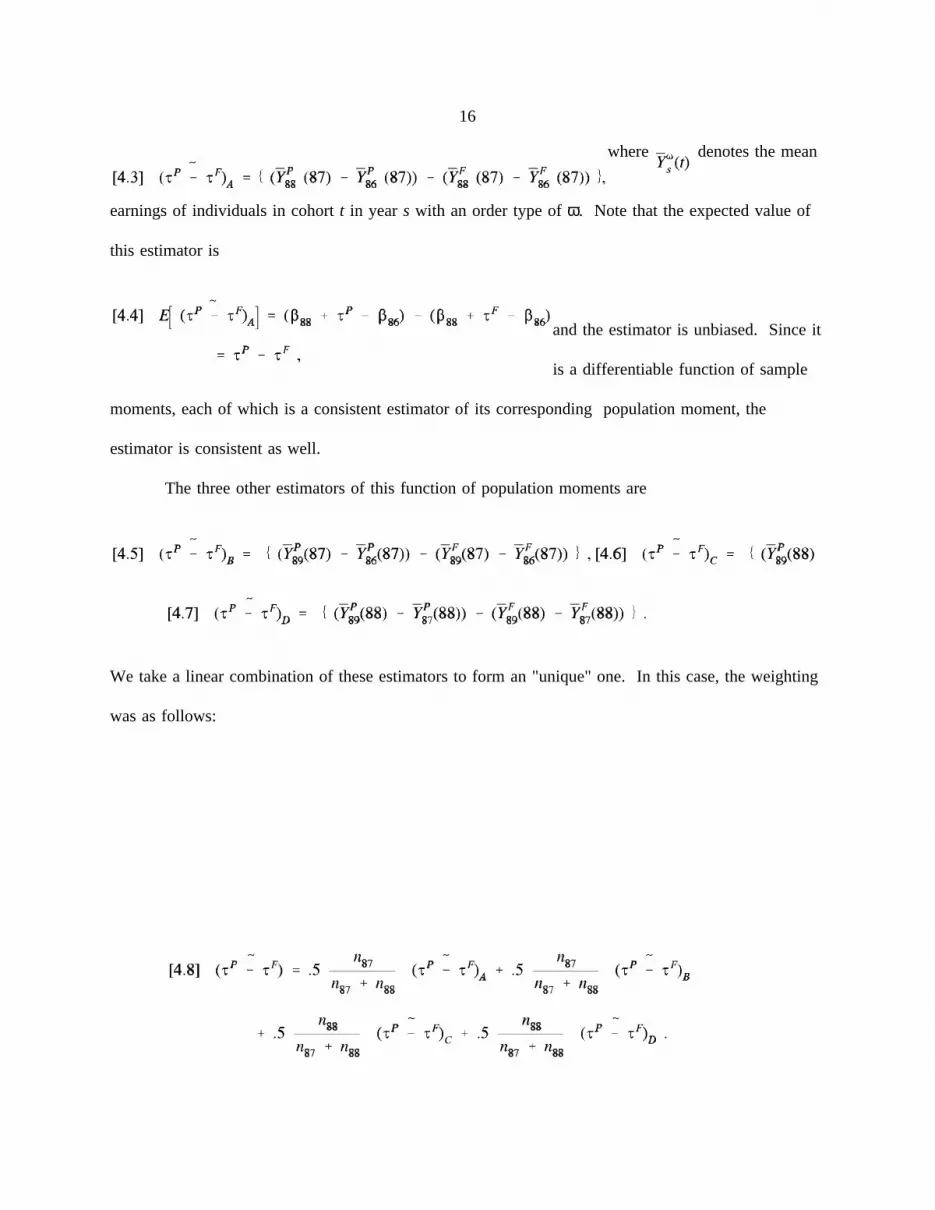
There exist four possible estimators of the function (τP-τF) given our data. One estimator is

10For surveys of issues related to the evaluation of welfare and training policies see Heckman andRobb (1985), Manski and Garfinkel (1992), and Barnow et al. (1980); this literature stressesidentification issues when using quasi-experimental data.

16

where denotes the mean

earnings of individuals in cohortt in years with an order type ofω. Note that the expected value of

this estimator is

and the estimator is unbiased. Since it

is a differentiable function of sample

moments, each of which is a consistent estimator of its corresponding population moment, the

estimator is consistent as well.

The three other estimators of this function of population moments are

We take a linear combination of these estimators to form an "unique" one. In this case, the weighting

was as follows:

17

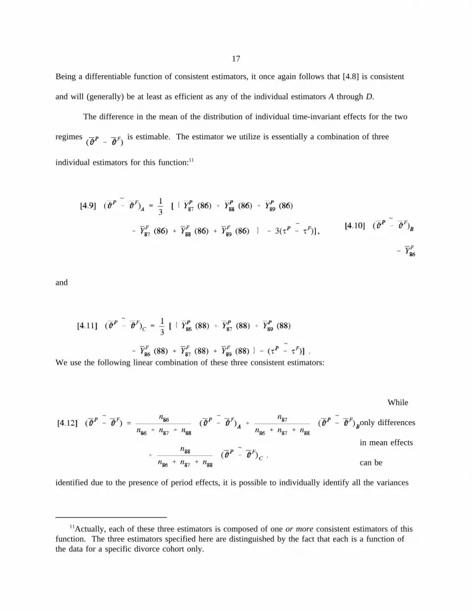
Being a differentiable function of consistent estimators, it once again follows that [4.8] is consistent

and will (generally) be at least as efficient as any of the individual estimatorsA throughD.

The difference in the mean of the distribution of individual time-invariant effects for the two

regimes is estimable. The estimator we utilize is essentially a combination of three

individual estimators for this function:11

and

We use the following linear combination of these three consistent estimators:

While

only differences

in mean effects

can be

identified due to the presence of period effects, it is possible to individually identify all the variances

11Actually, each of these three estimators is composed of oneor moreconsistent estimators of thisfunction. The three estimators specified here are distinguished by the fact that each is a function ofthe data for a specific divorce cohort only.

18

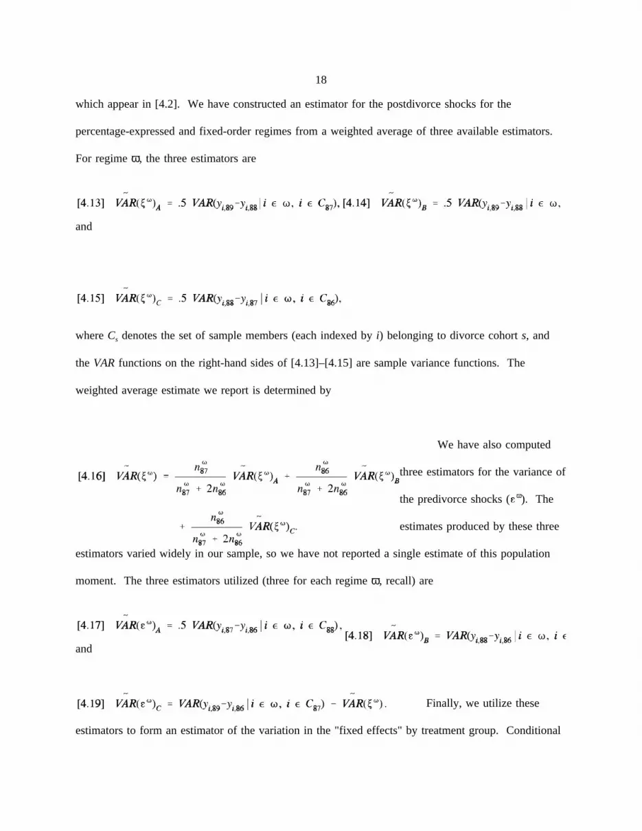
which appear in [4.2]. We have constructed an estimator for the postdivorce shocks for the

percentage-expressed and fixed-order regimes from a weighted average of three available estimators.

For regimeω, the three estimators are

and

whereCs denotes the set of sample members (each indexed byi) belonging to divorce cohorts, and

the VAR functions on the right-hand sides of [4.13]–[4.15] are sample variance functions. The

weighted average estimate we report is determined by

We have also computed

three estimators for the variance of

the predivorce shocks (ω). The

estimates produced by these three

estimators varied widely in our sample, so we have not reported a single estimate of this population

moment. The three estimators utilized (three for each regimeω, recall) are

and

Finally, we utilize these

estimators to form an estimator of the variation in the "fixed effects" by treatment group. Conditional

19

on consistent estimates of the variances of the predivorce and postdivorce shocks by treatment group,

we distinguish three estimators ofVAR(ϑω). They are:

and

The weighted average estimator of the variance of the fixed effect utilized is

Because we have three

estimates for the

predivorce shock

variance and the

estimator in [4.23] is a function of this particular variance estimate, we report three estimates produced

by [4.23], each corresponding to one of the three estimates of that parameter.

The method of moments estimates appear in the second column of Table 4.1, and a number of

interesting patterns in the income processes of divorced fathers emerge. First note that the differences

in the standard mean-shifting "treatment" effects between percentage-expressed and fixed orders is

negligible. The average income (in 1986 dollars) of fathers in the entire sample is approximately

$23,000 dollars, so that the difference in treatment effects of -356 is less than 2 percent of average

income.

21

TABLE 4.1

Methods of Moments Estimates of the Income-Generation Process, by Order Type

Parameter Estimator Defined In Point Estimate

[4.8] -355.799

[4.12] -3333.041

(A) [4.17] 19670.423(B) [4.18] 6222.016(C) [4.19] 5912.994

(A) [4.17] 5036.781(B) [4.18] 8764.308(C) [4.19] 9749.291

[4.16] 4708.506

[4.16] 7667.166

(A) [4.23] 11913.595(B) [4.23] 13450.379(C) [4.23] 13465.975

(A) [4.23] 17898.657(B) [4.23] 17758.606(C) [4.23] 17708.695

22

The fact that no treatment effects exist does not mean that mean earnings in the two treatments

are the same. We find that the difference in the mean fixed effects in the two groups is -3333,

approximately ten times the size of the treatment effect difference. Thus, while individuals with

percentage orders have significantly lower incomes than those with fixed orders postdivorce, the

differential is essentially maintained in the predivorce periods. On the basis of this evidence we

conclude that mean differences in the incomes of these groups are attributable to selection and not to

the order type per se.

The estimates of the standard deviations of the predivorce shocks display marked differences

across the two groups, though there is a large degree of instability of estimates across the three

estimators employed for each group. The estimator which is defined over differences only (estimator

A) produces an estimate of the standard deviation of the shock in the percentage-expressed group

which is roughly four times the size of the corresponding moment in the fixed-order group. However,

the other two estimators examined produce estimates of the standard deviation which are much larger

in the fixed-order group than in the percentage-order group. While we have not developed any

formal basis on which to compare the estimates, we have somewhat more confidence in the estimates

not based on differencing (the estimates obtained from estimatorsB andC). We shall come back to

an interpretation of these results after discussing the other variance estimates.

The standard deviation of the postdivorce shocks is significantly greater in the fixed-order

group than in the percentage-expressed group (7667 versus 4709). If divorced fathers with

percentage-expressed orders had an incentive to choose income-generation processes (jobs and/or

investment activities) with larger variances, we would expect to see the variance of the postdivorce

shock to increase relative to its predivorce level. In fact, the standard deviation of the postdivorce

shock is quite a bit less than its predivorce counterpart for percentage-order cases (from 19670, 6222,

or 5913 down to 4709). Thus there is no evidence that fathers with percentage orders choose riskier

23

income-generation processes, at least in the first few years after the divorce. The reduction in the

standard deviation of the earnings shock also occurs for fathers with fixed orders, at least under the

two estimates of this moment produced by estimatorsB andC.

The estimates of the variance of the individual effects in the two populations of fathers also

display easily noticeable differences. All of the estimates of the standard deviations of theϑP are no

more than 75 percent as large as corresponding estimates of the standard deviations of theϑF. Taken

together, the estimates of all of the standard deviations in the model indicate significantly more

dispersion in all of the random variables describing the dynamic income distribution of fathers with

fixed orders.

As was the case in the interpretation of the differences in means results, our estimates of the

variance components also seem to indicate a significant degree of selection in terms of order-type

assignment, with little behavioral effect of the program itself. The fathers with large amounts of

variability in their earnings processes are more likely to be given fixed orders than are those with more

stable earnings. If institutional actors have limited information about the father’s income history so

that it is impossible for them to disentangleϑ and , this selection mechanism also explains why the

variance in theϑ terms is greater for fathers under fixed orders. Selection-type arguments thus seem

to account for most of the results in Table 4.1, though why the variance of income shocks in the

postdivorce period is so much smaller than in the predivorce period (for both groups) remains

somewhat of a mystery.

5. REDUCED-FORM MODELS OF COMPLIANCE BEHAVIOR

In this section we examine the relationship between the characteristics of the child support

order, which include whether it is percentage expressed or fixed, whether withholding is in effect, the

size of the order, and the amount transferred from the father to the mother. The analysis contained

24

here is based on a simple econometric specification of the relationships between these characteristics

and transfers, and any attempt at explaining the mapping from order type to transfers in a behavioral

manner is postponed until Section 6. Nonetheless, in this empirical model we will examine some

issues relating to the possible endogeneity of the order characteristics in the child support transfer

regression function. The model specified here has the advantages of simplicity of statistical

interpretation of the results and comparability with previous empirical analyses in the literature.

For the moment, assume that all divorced fathers in the sample make positive child support

transfers,t, to the mothers. Denote the income of fathers byyf and the amount ordered bys. Let P

denote the indicator variable which is equal to 1 iff the father has a percentage-expressed order, and let

F ≡ 1-P. Similarly let W denote the indicator variable which is equal to 1 iff withholding is in effect,

and letN ≡ 1-W. We specify the transfer rule by

wherez is a row

vector of observable

covariates,γ is a conformable column vector, andu is a disturbance term which is mean-independent

of all right-hand-side variables with the possible exception of the indicator variables for order type

P,F and withholding status W,N.

Unlike the functions estimated by other researchers, the regression function we use has a few

unusual characteristics. First, note that aside from the indicator variables, the relationship betweent, s,

andyf is linear in the logarithms. From the point of view of examining compliance behavior, such a

specification has a potentially serious defect and one real strength. The defect is that the

transformation of the dependent variable,n(t), is not defined for cases in which the father makes no

transfer. While this would be a serious problem if one were examiningmonthlytransfer amounts, it is

not a serious problem in our data. First, the time unit of analysis is the year, and the proportion of

fathers who make no transfers over the year in the population of divorced fathers with child support

25

orders is relatively small. Second, this proportion is even smaller in the population of Wisconsin

fathers filing state income tax returns in the year following the divorce. From an original sample size

of 489 fathers, only 27 made no transfers over the year and were therefore excluded from the

following analysis.

Specification [5.1] has the advantage that the effects of orders on transfers, represented by the

ψ coefficients, have the interpretation of elasticities. Then the elasticity of transfers with respect to

orders clearly depends on which "regime" a father is in. Thus we can compare elasticities in a

straightforward way across regimes. For example, an increase of 1 percent in child support orders for

a father with percentage-expressed orders and subject to withholding results in an increase in transfers

of ψ1 percent. We will loosely interpret these elasticities as "compliance rates," as seems natural.

Besides being expressed in logarithms, [5.1] differs from other specifications used to

empirically determine the effect of percentage-expressed orders on transfers. For example, Bartfeld

and Garfinkel (1992) specify a regression function relating levels of transfers as a function of regime

and levels of orders, but do not include an interaction term between the two. While misspecification

of the relationship between orders, transfers, and regimes could possibly produce an essentially

"independent" effect of regime type on transfers, the global interpretation of such an effect presents a

problem.12 Clearly, we should expect the regime type to affect the rate of compliance with an order

of size s. In the regression function specification, this implies that an interaction term between the two

is the appropriate specification.

Given specification [5.1], we will be interested in testing for regime effects under the full

model and in two special cases. The special cases correspond to situations in which (1) there are no

interactions between the regime and the order amount (consistent with most previous empirical

12For example, the coefficients reported in Table 8 of Bartfeld and Garfinkel imply that having apercentage-expressed order increases the transfer by 111 dollars forany size order.

26

analyses of this issue) and (2) there are interaction effects with the order amount but no independent

effects of regime on the amount transferred. Since the general specification nests the two special

cases, it will be sufficient to specify the nature of the restrictions tested using [5.1].

We first test whether or not there are percentage-expressed order effects on transfer amounts

given withholding effects. In this case, the restrictions tested are

so there are four in all under the full model, two restrictions (β1 = β3 andβ2 =

β4) when the slope parameterψ is restricted to be the same across regimes, and

two restrictions (ψ1 = ψ3 andψ2 = ψ4) when the constant termβ is restricted to

be the same across regimes. As in all the cases considered in this section, the alternative hypothesis is

no restrictions on the regression parameters.

The restriction of no withholding effects given percentage-expressed-order effects is given by

As was the case above, there are four restrictions under the full model and two

each under the restricted models.

Finally, the null of no regime effects is given by

In this case there are six restrictions in the full model and three each in the

restricted versions.

Prior to estimating the model, testing for regime effects, and comparing

elasticities, it is necessary to consider the potential problem of endogeneity. In what follows we will

always consider the amount of the order to be exogenous with respect to the transfer decision. This

assumption is a practical necessity since this data set has a dearth of potential instrumental variables.

Therefore, we only consider the possibility that the regime may be endogenous. We first will examine

the issue of endogeneity of the order type conditional on the assumption of exogenously determined

withholding status. We then consider the endogeneity of withholding status conditional on the

27

assumption of exogenously determined order type. Finally, we test for endogeneity of order type and

withholding status simultaneously. The reader should bear in mind that the instrumental variable

procedures utilized below are strictly valid only under the assumption that the regime and the amount

of child support ordered are statistically independent.

To construct instruments for the regime type we use a simple index function approach. For

example, consider the case in which the order type is endogenous but withholding status is

exogenously determined. Then let the father be given a percentage-expressed order iff

wherex1 is a row vector of observable characteristics of the father,λ1 is a

conformable column vector of unknown parameters, andv1 is i.i.d. N(0,1). Then the probability that a

father is given a percentage-expressed order is simplyΦ(x1λ1), whereΦ denotes the standard normal

cumulative distribution functions. Maximum likelihood estimates ofλ1 are easily obtained from any

univariate probit procedure.

Next consider the case in which order type is exogenously determined but withholding status

is endogenous in [5.1]. In this case a father is assumed to be subject to withholding iff

wherev2 is i.i.d. N(0,1). The probability of withholding isΦ(x2λ2), and maximum likelihood estimates

of λ2 are straightforward to compute.

Finally consider the case in whichboth order type and withholding status are endogenously

determined. In such a case [5.5] and [5.6] are estimated simultaneously under the assumption that the

error terms are i.i.d. bivariate normal, where

Instruments are included in [5.1] in the following manner.

When only order type is considered endogenous, all occurrences of

the variableP are replaced with andF is replaced with , where is the maximum

28

likelihood estimate of from the univariate probit model. When only withholding status is

considered endogenous, all occurrences ofW are replaced with andN is replaced with

, where is the maximum likelihood estimate ofλ2 from the univariate probit model with

withholding status as the dependent variable. When both order type and withholding status are

considered endogenous, we use the following instruments for regime type:

where is the bivariate standard normal cumulative

distribution function indexed by correlation coefficientρ, and are maximum likelihood

estimates from the bivariate probit model.

It is of both substantive and technical interest to investigate the endogeneity issue even in this

reduced-form model. The endogeneity issue is interesting substantively in that it sheds light on the

nature of the selection mechanism, which in this case involves the behavior of institutional actors and

divorced parents. This particular approach to looking at the selection issue has not been utilized

previously in addressing the question of the effect of order characteristics on transfers and/or

compliance.13 Pragmatically, it is of interest to determine whether it is necessary to use instrumental

variables, since due to the lack of good potential instruments there is likely to be a large loss in

efficiency if they are used in situations where they are not required for purposes of consistency.

13Bartfeld and Garfinkel utilize an inverse Mills ratio approach to correct for selection, though thisapproach is valid under more stringent conditions on the joint distribution of the disturbances in [5.1]and [5.7] than are required under the procedure we utilize. Furthermore, they treat withholding statusas exogenous throughout.

29

To test for endogeneity we use the "omitted variable" method developed by Durbin (1954),

Wu (1973), and Hausman (1978) and nicely described in Godfrey (1988). The endogeneity test

amounts to adding the estimated regime probabilities to specification [5.1] and then performing a test

to determine whether all the coefficients associated with the predicted probabilities are jointly equal to

zero. For example, when we consider the situation in which withholding status is taken to be

exogenous with order type (potentially) endogenous, we estimate

by ordinary least

squares (OLS).

Using the Eicker-White heteroskedasticity-consistent standard errors, we then test whether the OLS

estimates ofα1 andα2 are jointly equal to zero. If there is little evidence to reject this null, we

conclude that it is likely that order type is not endogenous. The reader should bear in mind that the

test is likely to have relatively low power when the quality of the instruments utilized is poor, as is the

case here. Similar specifications are estimated and tests conducted for the withholding-only

endogenous case and the joint endogeneity case.

For the reduced-form compliance estimates, we utilize a sample of divorced fathers who

satisfied the following criteria: (1) received child support orders in 1986, 1987, or 1988; (2) filed a

State of Wisconsin income tax return for the year following the one in which they received their child

support order; (3) had child support order information for the calendar year following the receipt of

the order; (4) had valid child support transfer information for the year following the divorce; and (5)

made positive transfers to the mother during the year following the divorce. Prior to imposing

condition (5) there were 489 valid cases from the WCRD; imposition of (5) resulted in a small loss of

27 cases.

30

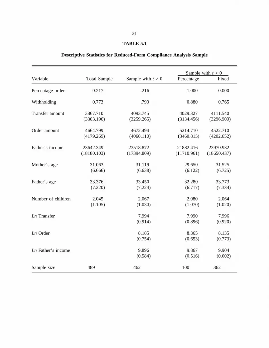
Descriptive statistics for this sample are contained in Table 5.1. First note from a comparison

between columns 1 and 2 of the table that the proportion of percentage-order cases is virtually

identical both before and after cases with zero transfers are excluded. On the other hand, cases with

withholding are slightly overrepresented when we impose the positive transfer requirement, which

seems reasonable. In column 2, we see that approximately 22 percent of the individuals in the sample

have percentage-expressed orders (100 cases). The majority of cases, 79 percent, are subject to

mandatory withholding. The ratio of average transfers to average orders is approximately .88. The

ratio of average orders to average income is about .20. Note that all monetary amounts expressed

throughout the paper are denominated in terms of 1986 dollars.

Columns 3 and 4 of the table give sample statistics for the percentage-expressed and

fixed-order groups. A larger proportion of fathers with percentage-expressed orders are subject to

withholding. For the percentage-expressed cases, average orders are slightly higher while average

incomes are slightly lower (which is known from the estimates in Section 3). In other respects, such

as age and number of children, the fathers in the two regimes are similar. Fathers with

31

TABLE 5.1

Descriptive Statistics for Reduced-Form Compliance Analysis Sample

Sample witht > 0Variable Total Sample Sample witht > 0 Percentage Fixed

Percentage order 0.217 .216 1.000 0.000

Withholding 0.773 .790 0.880 0.765

Transfer amount 3867.710 4093.745 4029.327 4111.540(3303.196) (3259.265) (3134.456) (3296.909)

Order amount 4664.799 4672.494 5214.710 4522.710(4179.269) (4060.110) (3460.815) (4202.652)

Father’s income 23642.349 23518.872 21882.416 23970.932(18180.103) (17394.809) (11710.961) (18650.437)

Mother’s age 31.063 31.119 29.650 31.525(6.666) (6.638) (6.122) (6.725)

Father’s age 33.376 33.450 32.280 33.773(7.220) (7.224) (6.717) (7.334)

Number of children 2.045 2.067 2.080 2.064(1.105) (1.030) (1.070) (1.020)

Ln Transfer 7.994 7.990 7.996(0.914) (0.896) (0.920)

Ln Order 8.185 8.365 8.135(0.754) (0.653) (0.773)

Ln Father’s income 9.896 9.867 9.904(0.584) (0.516) (0.602)

Sample size 489 462 100 362

32

percentage-expressed orders are slightly younger, which may be related to the increasing trend in

percentage-expressed-order awards over this period (1986–1988).

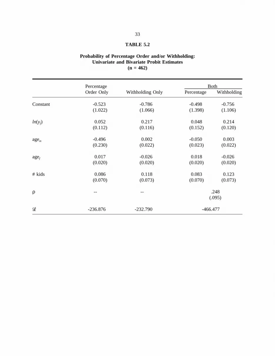
Table 5.2 contains probit estimates of regime probabilities. Column 1 contains univariate

probit estimates of the model in which the dependent variable is the percentage-expressed-order

indicator. The logarithm of the father’s income in the yearfollowing the divorce is used in the

estimation exercise, because this is the only income variable included in this extract. Since Section 4

demonstrated that there is no systematic effect of order type on the mean level of the income process,

this income measure is probably a reasonably good proxy for the father’s income at the time the child

support award was determined. We see that conditional on parental ages and number of children,

there is a positive relationship between income and the probability of a percentage-expressed order,

though the effect is not statistically significant. The only parameter estimate more than twice its

standard error is the age of the mother, which is negatively related to the receipt of a

percentage-expressed order.

Column 2 contains estimates of the univariate probit model in which the withholding indicator

is the dependent variable. Fathers with higher incomes are more likely to be subject to withholding,

quite possibly because they have more stable employment patterns and thus are easier to subject to

withholding in the first place. Fathers with larger numbers of children are also more likely to be

subject to withholding.

Columns 3 and 4 contain estimates from the bivariate probit specification. The pattern of the

coefficient estimates ofλ1 andλ2 is virtually unchanged from the univariate results. The error term in

the latent variable expression for percentage-expressed orders,v1, is positively correlated with the error

term in the latent variable expression for withholding,v2. Furthermore, the correlation coefficient is

statistically different from zero at conventional significance levels. Allowing for a

33

TABLE 5.2

Probability of Percentage Order and/or Withholding:Univariate and Bivariate Probit Estimates

(n = 462)

Percentage BothOrder Only Withholding Only Percentage Withholding

Constant -0.523 -0.786 -0.498 -0.756(1.022) (1.066) (1.398) (1.106)

ln(yf) 0.052 0.217 0.048 0.214(0.112) (0.116) (0.152) (0.120)

agem -0.496 0.002 -0.050 0.003(0.230) (0.022) (0.023) (0.022)

agef 0.017 -0.026 0.018 -0.026(0.020) (0.020) (0.020) (0.020)

# kids 0.086 0.118 0.083 0.123(0.070) (0.073) (0.070) (0.073)

ρ -- -- .248(.095)

-236.876 -232.790 -466.477

34

nonzero correlation between thev’s significantly improves the predictive power of the model, which is

especially important for the construction of good instruments.

As indicated above, we used the probit estimates to construct instruments for the variables that

indicate regime. These instruments were used in conducting endogeneity tests, and the results are

reported in Table 5.3. Generally speaking, we found little evidence of endogeneity in the nine

specification tests run. To interpret the results, consider the entry in column 1, row 3, which

corresponds to the test of percentage-order endogeneitygivenwithholding-status exogeneity when the

full model is estimated. The "full model" corresponds to specification [5.1] in which regimes can

have effects both on the intercept and the slope (with respect ton(s)) in the n(t) function. In this

case [5.9] was estimated, and the null of exogeneity implies two restrictions on this equation. The test

statistic was found to be 2.824, which is distributed as a random variable under the null. The

probability of this value is .244, indicating that percentage orders, given exogenous withholding, are

best considered exogenous in the transfer regression.

Across all six specifications in which regimes can affect constants or slopes but not both (the

first two rows of Table 5.3), there is no evidence of endogeneity. Only when the regime can shift

both the constantand the slope parameter is there any indication of endogeneity. In particular, the test

for joint endogeneity of order type and withholding status in the full model produces a test statistic of

19.576, which has a probability of only .003 under the null of joint exogeneity. Aside from the results

of this particular test, however, there is little evidence of endogeneity of regime type in the transfer

regression. Therefore, we will focus our attention on the interpretation of the estimated version of

[5.1] when instruments are not used.

35

Regression results are reported in Table 5.4. In the first column, OLS estimates of the

restricted model in which regime type only shifts the intercept in then(t) regression function are

presented. Note that the coefficient associated withn(s) is .879, holding constant the father’s

35

TABLE 5.3

Endogeneity Tests of Percentage Order and/or Withholding:Test Statistics with Degrees of Freedom in [ ] and Probability under Exogeneity in ( )

Instrumented Variable(s)Regime Effects Percentage Order Withholding Both

Constants only 2.083 0.013 2.320[1] [1] [3](0.149) (0.910) (0.509)

Slopes only 2.276 0.077 1.170[1] [1] [3](0.131) (0.781) (0.760)

Constants and slopes 2.824 4.709 19.576[2] [2] [6](0.244) (0.095) (0.003)

36

TABLE 5.4OLS Regressions ofLn(t)

(Eicker-White Standard Errors)

1 2 3

Constant -0.978(0.536)

P*W -1.077 -0.268(0.537) (0.740)

P*N -1.349 -2.593(0.569) (1.498)

F*W -0.852 -1.745(0.551) (0.532)

F*N -1.090 0.049(0.532) (0.995)

n(yf) 0.177 0.182 0.210(0.066) (0.065) (0.064)

n(s) 0.879(0.048)

n(s)*P*W 0.861 0.743(0.047) (0.095)

n(s)*P*N 0.830 0.991(0.050) (0.176)

n(s)*F*W 0.890 0.948(0.048) (0.052)

n(s)*F*N 0.858 0.696(0.051) (0.115)

Tests of Regime Effects

No percentage order effect 10.510 11.125 14.325[2] [2] [4](0.005) (0.004) (0.006)

No withholding effect 10.938 11.491 16.565[2] [2] [4](0.004) (.003) (.002)

No percentage order or withholding effect 25.193 27.721 39.421[3] [3] [6](<0.001) (<0.001) (<0.001)

37

income. Under our interpretation, a 1 percent increase in the ordered amount results in an .88 percent

increase in transfers to the mother. Also, for every 1 percent increase in the father’s income the

transfer amount increases by .18 percent, holding constant the order. This is interesting because the

standard order percentage for fathers with one child is 17 percent. One interpretation of this estimate

is that this is the proportion of their income divorced fathers would choose to contribute to the mother

even given ordered amounts.

In column 2 we present the estimates of the restricted model in which the regime only affects

the elasticity of payments with respect to orders, or loosely speaking, the compliance rate. Note that

the highest "compliance rate" (.89) is associated with fixed orders and withholding, while the lowest

(.83) is associated with percentage-expressed orders without withholding. (This latter group comprises

less than 3 percent of this sample.) Percentage orders with withholding and fixed orders without

withholding have approximately the same coefficients.

The regression estimates in column 3 indicate that among the more precisely estimated regime

effects (that is, excluding the regimeP N), the fixed order with withholding regime continues to be

the highest compliance regime. In terms of effects of the regime on the intercept, fixed orders without

withholding have the largest coefficient.

The test statistics for the various regime effects are reported at the bottom of the table. In

general, the tests reveal strong regime effects no matter what the specification of the test. The

characteristics of the order are an important determinant of the amount transferred.

Table 5.5 contains estimation and testing results when the regimes are replaced with

instruments. Because the instruments are relatively poor, all estimates are quite imprecise (that is,

have large associated standard errors). Due to this fact, it is difficult to compare the results in this

table with those in Table 5.4. Since there was little evidence for endogeneity, we believe that the

results in Table 5.4 better reflect the reduced-form relationship between transfers, order regimes,

38

TABLE 5.5OLS Regressions ofLn(t) with Instruments for Regimes

(Eicker-White Standard Errors)

1 2 3

Constant -0.629(0.713)

-1.696 -9.590

(1.131) (11.074)

4.623 -17.369

(6.081) (62.958)

0.153 4.223

(0.975) (3.286)

-2.156 -4.655

(1.047) (8.276)

n(yf) 0.164 0.173 0.172(0.075) (0.076) (0.078)

n(s) 0.841(0.047)

n(s)*P W 0.725 1.714

(0.151) (1.350)

n(s)*P N 1.432 4.175

(0.822) (8.138)

n(s)*F W 0.912 0.355

(0.078) (0.432)

n(s)*F N 0.665 1.082

(0.169) (1.115)

Tests of Regime Effects

No percentage order effect 3.484 1.719 15.780[2] [2] [4](0.175) (0.423) (0.003)

No withholding effect 1.554 0.823 4.726[2] [2] [4](0.460) (.663) (.317)

No percentage order or withholding effect 3.485 1.722 16.559[3] [3] [6](0.323) (0.632) (0.011)

39

order amounts, and father incomes. On the basis of these results, we conclude that the effects of order

regime on the transfers and welfare levels of divorced parents should concern shapers of child support

policy.

6. BEHAVIORAL MODELS OF CHILD SUPPORT TRANSFERS UNDERPERCENTAGE-EXPRESSED AND FIXED ORDERS

The evidence from the reduced-form analysis of the compliance decision generally supported

the idea that there were lower levels of compliance with percentage-expressed orders than fixed orders,

holding the income of the custodial parent and the child support order constant, at least when both

were combined with withholding. We also found that the effect of order type on transfer cannot be

captured solely through intercept terms. In this section we estimate a structural model of child support

transfers with a nontrivial compliance decision. This work extends our earlier research on compliance

(Del Boca and Flinn 1993) to consider the differential effects of order type on the transfer process.

Using this model, in principle we can determine whether fathers with percentage-expressed orders

differ from fathers with fixed orders in terms of their relative preferences for own versus child

consumption and/or in terms of the distribution of costs of noncompliance. The implications of the

previous section’s results appear to be that the preference characteristics of the fathers are not

significantly different in the two order regimes (indicated by the lack of significance of the

endogeneity tests of order type in the transfer regressions), but that the costs of noncompliance vary

by regime. We will be interested in determining whether the structural model estimates are consistent

with this interpretation.

To motivate our analysis, we first present the empirical distributions of child support awards

and payments in the data utilized below. All amounts are expressed in monthly terms and in 1986

dollars. In Figure 6.1 we present the distribution of child support orders in our sample of 282 fathers

40

(222 with fixed orders and 60 with percentage-expressed orders). Figure 6.2 contains the distribution

of actual child support transfers from the noncustodial father to the custodial mother; with respect to

the distribution of orders, it tends to be "compressed" toward the origin. Figure 6.3 contains the

distribution of the ratio of payments to orders. This distribution is interesting in that while the spikes

at 0 and 1 (corresponding to what we will refer to later asexactcompliance) are its predominate

feature, a significant proportion of individuals make positive payments less than the amount ordered

and a smaller proportion make payments greater than the ordered amount. The model we describe and

estimate below will be able to capture these qualitative features of the distribution in a parsimonious

manner.

Figures 6.4 through 6.6 are analogous to 6.1 through 6.3 but refer solely to the subsample of

fathers with percentage-expressed orders. Because this sample is so small, it is difficult to draw many

strong conclusions from these histograms, though it does appear that the distribution of transfers is a

bit more "compressed" toward the origin than was the case for the entire sample. This impression

persists when we compare it with the corresponding histograms for the subsample of fathers with fixed

orders, which are contained in Figures 6.6 through 6.9.

Throughout the analysis, we will assume that the mother is the custodial parent. We begin by

examining the behavior of divorced parents in an environment without child support orders. Though

the divorced parents no longer inhabit the same household and are assumed to have access to two

independent sources of income, denotedym andyf, their welfare is connected after the divorce due to

the presence of the public good, the child. Letcp denote the private consumption of parentp, and letk

denote the consumption of the child. Then the utility function of parentp is assumed to be

Cobb-Douglas, so

41

Figures 6.1 through 6.3 here

42

Figures 6.4 through 6.6 here

43

Figures 6.7 through 6.9

44

A critical assumption concerns the manner in which the consumption level of the child is set. Because

the mother has both physical and legal custody, we assume that all "significant" expenditures on the

child must be made or approved by her. We take the extreme position that the only way in which the

father may augment the consumption level of the child is by transferring money to the mother. Given

the father’s transfer and her own income, the mother freely allocates it on her own consumption and

that of the child.14

Without loss of generality, we will normalize the price of the private consumption goods of

the parents and the child to unity. Given her total income levelym + t, wheret is the transfer from the

father, the mother then chooses a level of expenditure on the child equal to

. The father, taking the mother’s behavior as predetermined,

chooses his transfer to the mother according to:

Due to the functional forms

with which we are

working, it is also easily seen that the optimal transfer of the father to the mother is independent of the

value of the mother’s preference parameter, so for all values ofδm.

The decision rule is characterized by

whereyt = ym + yf is aggregate parental income.

The assumption that only mothers can

directly make expenditures on "child goods" leads to the prediction that we would observe positive

14In a dynamic model, the mother’s choices in any periodt may elicit behavioral responses fromthe father in later periods which she would consider in setting expenditure levels for periodt. In sucha situation, we might observe different choices of expenditure levels on child consumption by custodialmothers with the same levels of total income but different amounts of child support income (see Flinn[1994]). However, in a static model such as the one analyzed here, such feedback is ruled out andmothers have no behavioral or legal reason for treating the two income sources differently in makingexpenditure decisions.

45

transfers from fathers to mothers even in the absence of child support awards. Because the amount of

the child support award appears nowhere in the specification, this model of transfers leads to no

interesting implications regarding compliance behavior. To rectify this situation, we modify the

preferences of the father so as to produce the utility function

wheres is the order, [ζ] is an indicator function

which takes the value 1 when logical expressionζ is true and 0 when it is not, andϑ is a fixed cost

that the father pays if he does not fully comply with the order.15 The penalty may be in the form of

income reductions (due to fines, interest payments on child support owed, and/or the loss of work time

due to incarceration) or in the reduction of time spent with the child.

Let us now examine the utility levels in states of exact compliance and the utility when the

transfert* is made. Whether "exact" compliance occurs or not depends solely on the sign of the

difference between the utility of noncompliance and compliance . We will

examine this difference for five qualitatively distinct cases, distinguished by values of the father’s

preference parameterδf and the noncompliance cost parameterϑ. For reference, we also present a

more formal characterization of these cases in Figure 6.10.

We first consider the case in which the father’s preference parameter is greater than or equal

to his share of total parental income, that is, the case of maximum "selfishness." In this case, if there

were no noncompliance cost, the father would choose to transfer nothing to the mother. Then if the

father does not comply with the order, he will transfer zero. If he chooses to comply (because the

15The addition of this type of random variable to account for differential levels of programparticipation or noncompliance within a homogeneous population is common in the literature (see, e.g.,Moffitt [1983]).

46

FIGURE 6.10

Utilities and Transfers under Different Choices

Father’s Preferences Utility Transfer

s

0

Choice depends on:

______________________________________________________________________

s

0 < t* < s

Choice depends on:

______________________________________________________________________

t* > s

47

noncompliance costϑ is large), he will transfer the minimum amount necessary to avoid the

noncompliance cost, which is the orders. Then for any value ofδf in the interval [yf /yt,1], there exists

a unique value of the noncompliance costD0(δf) such that for any value ofϑ greater thanD0(δf), the

father will transfers; for ϑ ≤D0 (δf), the father will transfer nothing. These are the first two

qualitatively distinct cases.

The next two cases correspond to the situation in which the father’s preference parameter lies

in the interval [(yf -s)/yt, yf /yt]. In this case, even if the noncompliance cost is zero, the father would

choose to transfer a positive amount to the mother,but an amount less than the orders. Once again,

for any value ofδf in this interval, there will exist a unique valueD1(δf) such that ifϑ > D1(δf), the

father will avoid the noncompliance cost and transfer the orders; if ϑ ≤ D1(δf), the father will transfer

a positive amount less than the order. In this latter case, we will say that the father "partially"

complies.

The final case is the simplest to describe. Ifδf ≤ (yf -s)/yt, the father would optimally choose

to transfer at least the amount of the order. Thus the child support order is not a binding constraint

from the point of view of the father, and fathers in this situation will be said to "overcomply."

Figure 6.10 provides a summary of the three cases for a given parental income distribution (ym,

yf) and a given orders. It is clear that if the distribution ofδf in the population has support equal to

[0,1], and if the cost of noncompliance parameterϑ is sufficiently "dispersed" (in a sense to be made

precise below), this model of the transfer decision in principle has the capability to explain the

observed fact of the simultaneous existence of no transfers, partial compliance, exact compliance, and

overcompliance evidenced in the data.

The sample can be thought of as being comprised of four classes of individuals, which are

[C1] those fathers making no payment in the year, ort = 0; [C2] those fathers "partially complying" in

the sense of making a transfer which is positive but less than the stipulated amount, or 0 <t < s; [C3]

48

those fathers making a payment exactly equal to the stipulated amount, ort = s; and [C4] those fathers

"overcomplying" in the sense of making a transfer which is greater than the stipulated amount, ort >

s. The contributions of members of these groups to the sample likelihood function are presented in

Appendix A.

With all the required pieces defined, the sample log likelihood function is given by

whereψG is a

finite-dimensional parameter vector which completely determines the distribution function of the

preference parameterδf in the population of noncustodial fathers, and withψH denoting the

finite-dimensional parameter vector which completely characterizesH.

The model is completely characterized by the parameters which describe the distributions of

the father’s preference parameter and the direct cost of noncompliance. Let Then the

maximum likelihood estimate of the parameter vectorψ is given by , whereΩ is

the parameter space, the characteristics of which are determined by the functional forms of the

distribution functionsG andH.

For the econometric model to be logically consistent, we must restrict our choice ofG, the

distribution of the direct cost of noncompliance, to those parametric distributions which have support

on the positive real line. Similarly, our choice ofH must come from the set of parametric

distributions which have support on the unit interval. Pragmatically, the distributions we choose must

be characterized by a very low dimensional parameter vector if we are to have any hope of precisely

estimating the parameter vectors characterizing the distributions. This is especially true with respect to

the distribution ofϑ, since this random variable is never directly observed. In the case of the random

variableδf, its value is directly imputable for the portion of the sample which partially complies or

49

overcomplies; for this reason, we can expect precise estimation ofψH to be an easier task than forψG

whenψG andψH are similarly dimensioned.

We have estimated the econometric model under the assumption that the distribution of the

father’s preference parameterδf is of the form of a two-parameter beta. A beta distributed random

variable takes values on the interval [0,1], and the distribution is quite "flexible." We assume that the

distribution of the cost of noncomplianceϑ is exponential (and so is characterized by one parameter).

Under these distributional assumptions, the log likelihood function is characterized by three

parameters, and the parameter spaceΩ = . The log likelihood is continuously differentiable over

the interior of the parameter space, and all standard regularity conditions for consistency and

asymptotic normality of the maximum likelihood estimator ofθ will be satisfied provided that the true

parameter vectorψ0 is an interior point ofΩ. While (ψ) is not globally concave overΩ, we found

that the maximum likelihood estimates reported below were attained no matter which point inΩ was

used as a starting value in the optimization algorithm.16

Descriptive statistics for the sample used in this section are presented in Table 6.1.

Characteristics of this sample are broadly consistent with those of the sample used in the reduced-form

compliance analysis. The additional sample selection requirement that the mother also file a state

income tax return has resulted in a sample with a slightly higher mean income (for the fathers) and

slightly higher order amounts.

Because the data on orders and transfers are highly time-aggregated, and because the structural

parameter estimates from this model of compliance tend to be quite sensitive to the proportion of the

sample which "exactly" complies, we estimated the model after defining individuals with transfer/order

16For each of the four sets of model estimates reported below, between five and ten diverse startingvalues were used.

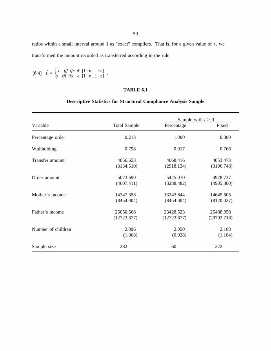
50

ratios within a small interval around 1 as "exact" compliers. That is, for a given value of , we

transformed the amount recorded as transferred according to the rule

TABLE 6.1

Descriptive Statistics for Structural Compliance Analysis Sample

Sample witht > 0Variable Total Sample Percentage Fixed

Percentage order 0.213 1.000 0.000

Withholding 0.798 0.917 0.766

Transfer amount 4056.653 4068.416 4053.473(3134.510) (2918.134) (3196.748)

Order amount 5073.690 5425.010 4978.737(4607.411) (3288.482) (4905.300)

Mother’s income 14347.358 13243.844 14645.605(8454.004) (8454.004) (8120.027)

Father’s income 25050.568 23428.523 25488.958(12723.677) (12723.677) (20702.718)

Number of children 2.096 2.050 2.108(1.068) (0.928) (1.104)

Sample size 282 60 222

51

where is our modified transfer used in the estimation exercise. Varying can of course have large

effects on the estimates obtained.

Prior to applying [6.4] to the raw data, we consider the distribution of the sample in the

interval [1- , 1+ ] for various values of . Table 6.2 reports the numbers and proportion of

individuals according to different ratios of transfers to orders. Only five individuals (under fixed

orders) can be classified as perfect compliers for = 0. When we widen the interval from .95 to 1.05,

we find 18 percent of the percentage-order and 41 percent of the fixed-order cases. When increases

to .25 these percentages increase to 52 and 76 respectively.

Table 6.3 presents the estimates of the structural compliance model, when "exact" compliance

is defined ast/s ε [.95, 1.05]. Four specifications are presented for the estimates of the distributions of

δf andϑ. Under specificationI, separate distributions for the noncompliance cost and preference

parameter distribution are estimated for the fixed-order and percentage-expressed-order groups. The

point estimates indicate that the fathers are not very different in their preference characteristics, but

that noncompliance costs are on average lower in the population of fathers with percentage-expressed

orders.

Under specificationII , the preference distributions are restricted to be the same in the two

populations, while the noncompliance cost distributions are allowed to differ. In specificationIII the

noncompliance cost distribution is restricted to be the same but the preference parameter distributions

are allowed to differ. Finally, inIV all distributions are restricted to be the same. A comparison of

the likelihood values indicates that there is virtually no statistically significant difference in the

preferenceand noncompliance cost distributions for the two groups. This is a negative result from the

perspective of consistency with our earlier findings, but one that was not totally unexpected a priori.

The structural model relies on rather intricate nonlinearities in the data for identification of the

behavioral distributions. With so few observations, sixty in the case of the percentage-expressed-order

52

TABLE 6.2

Numbers and Percentage of Individuals in Structural Estimation Samplewith t/s Ratio in Selected Intervals

t/s Interval Number of Individuals Percentage of Sample

[1.000, 1.000] 5 0.018[0] [0.000](5) (0.023)

[0.975, 1.025] 71 0.252[5] [0.083]

(66) (0.297)

[0.950, 1.050] 102 0.362[11] [0.183](91) (0.410)

[0.900, 1.100] 147 0.521[15] [0.250]

(132) (0.595)

[0.850, 1.150] 172 0.610[23] [0.383]

(149) (0.671)

[0.750, 1.250] 200 0.709[31] [0.517]

(169) (0.761)

Notes: N = 282. Percentage orders are in [ ]; fixed orders are in ( ).

53

TABLE 6.3

Estimates of Structural Compliance Model, with Exact Compliance Defined ast/s ε [.95, 1.05]

SpecificationI II III IV

Parameter P F P F P F

Distribution of the Father’s Cobb-Douglas Utility Parameter (δf)

ψ1 2.717 3.520 3.296 1.392 3.543 3.294(1.251) (0.631) (0.549) (0.417) (0.628) (0.549)

ψ2 1.851 1.672 1.626 2.546 1.690 1.625(1.115) (0.388) (0.353) (1.154) (0.387) (0.353)

E(δf) 0.595 0.678 0.670 0.353 0.677 0.670

SD(δf) 0.208 0.188 0.193 0.215 0.187 0.193

Distribution of the Noncompliance Cost Parameter (ϑ)

ψ3 2.006 1.329 1.634 1.340 1.664 1.375(1.699) (0.425) (1.236) (0.426) (0.975) (0.410)

E(ϑ) 0.499 0.752 0.612 0.746 0.601 0.727

-623.614 -624.833 -623.714 -624.861

Note: Restricted parameters are in boldface.

54

group, lack of statistical significance is not surprising. Our conjecture is that if the sample size were

increased to more reasonable levels, say on the order of 1000, statistically significant differences in the

noncompliance cost distribution, and possibly the preference distribution, would emerge. Since the

statistically insignificant differences here are broadly consistent with results from Section 5, we view

the two exercises as complementary.

Table 6.4 repeats the estimation exercise for the case in which "exact" transference is defined

for all t/s ratios in the interval [.9,1.1]. Since there is more "compliance" by definition in this sample,

it is not surprising to see that the estimates reflect a shift in the noncompliance cost distribution

toward larger values. This occurs for both percentage-expressed and fixed orders. On the other hand,

the preference parameter distribution is relatively unaffected by the change in the definition of

noncompliance. Statistical tests across the four specifications in Table 6.4 yield the same conclusions

as we drew from Table 6.3. Distributional differences are statistically insignificant, but the costs of

noncompliance appear quite a bit higher for fathers with fixed orders.

7. CONCLUSIONS

In this paper we have investigated the effects of fixed and percentage-expressed child support

orders on the income of noncustodial fathers and child support transfer decisions. The results of the

statistical model of the income-generating process of fathers before and after divorce show small

effects of the type of order on postdivorce income, but indicate nonrandom assignment of the type of

order.

The evidence from the reduced-form analysis of the compliance decision generally supported

the idea that there were lower levels of compliance with percentage-expressed orders than fixed orders,

holding the income of the custodial parent and the child support order constant, at least when both

were subject to withholding. We have also used a structural model of child support compliance

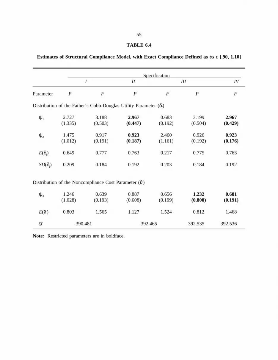
55

TABLE 6.4

Estimates of Structural Compliance Model, with Exact Compliance Defined ast/s ε [.90, 1.10]

SpecificationI II III IV

Parameter P F P F P F

Distribution of the Father’s Cobb-Douglas Utility Parameter (δf)

ψ1 2.727 3.188 2.967 0.683 3.199 2.967(1.335) (0.503) (0.447) (0.192) (0.504) (0.429)

ψ2 1.475 0.917 0.923 2.460 0.926 0.923(1.012) (0.191) (0.187) (1.161) (0.192) (0.176)

E(δf) 0.649 0.777 0.763 0.217 0.775 0.763

SD(δf) 0.209 0.184 0.192 0.203 0.184 0.192

Distribution of the Noncompliance Cost Parameter (ϑ)

ψ3 1.246 0.639 0.887 0.656 1.232 0.681(1.028) (0.193) (0.608) (0.199) (0.808) (0.191)

E(ϑ) 0.803 1.565 1.127 1.524 0.812 1.468

-390.481 -392.465 -392.535 -392.536

Note: Restricted parameters are in boldface.

56

to investigate whether fathers with percentage-expressed orders differ from fathers with fixed orders in

terms of their relative preferences for own versus child consumption and/or in terms of the distribution

of costs of noncompliance. The inferences to be drawn from these results are more or less consistent

with those obtained from the reduced-form estimates.

In the future we hope to develop the behavioral model so as to model the cost of

noncompliance distribution in a more satisfactory manner. With larger samples, and using more

information from the court records associated with these data, we would like to more specifically

define costs of noncompliance (for example, in terms of court appearances and sanctions) so as to

isolate the characteristics of percentage-expressed orders which make them more difficult to enforce

than fixed orders.

57

APPENDIX A

Likelihood Function for the Four Groups of Fathers

C1: No Transfer

Only those fathers with preference parameter would make no transfer if it were not

stipulated. Conditional on and the characteristicsy ands, the probability of

noncompliance is given by

whereψG is a finite-dimensional parameter vector which completely characterizes the distribution

function G, and where WithH

denoting the distribution function of the preference parameterδf in the population of noncustodial

fathers, and withψH denoting the finite-dimensional parameter vector which completely characterizes

H, the probability of zero payment for a father with characteristics (y,s) is

This probability represents the contribution of a member ofC1 to the sample likelihood, which we will

denoteLC1.

C2: Partial Compliance

The probability that such an individual will not comply with the order is given by

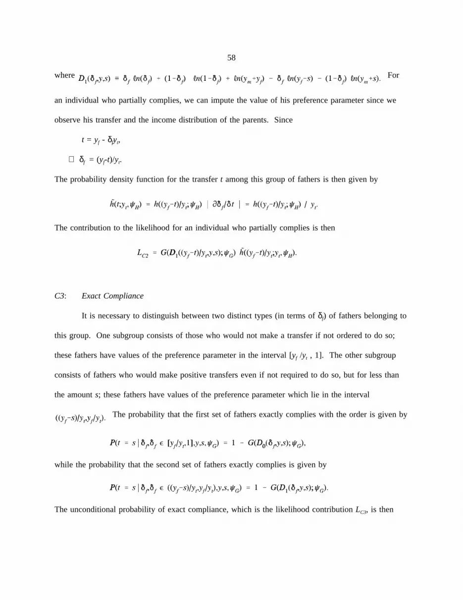
58

where For

an individual who partially complies, we can impute the value of his preference parameter since we

observe his transfer and the income distribution of the parents. Since

t = yf - δfyt,

⇒ δf = (yf-t)/yt.

The probability density function for the transfert among this group of fathers is then given by

The contribution to the likelihood for an individual who partially complies is then

C3: Exact Compliance

It is necessary to distinguish between two distinct types (in terms ofδf) of fathers belonging to

this group. One subgroup consists of those who would not make a transfer if not ordered to do so;

these fathers have values of the preference parameter in the interval [yf /yt , 1]. The other subgroup

consists of fathers who would make positive transfers even if not required to do so, but for less than

the amounts; these fathers have values of the preference parameter which lie in the interval

The probability that the first set of fathers exactly complies with the order is given by

while the probability that the second set of fathers exactly complies is given by

The unconditional probability of exact compliance, which is the likelihood contributionLC3, is then

59

C4: Overcompliance

The likelihood contribution for members of this group is simply

The likelihood function is then

60

References

Barnow, B. S., G. G. Cain, and A. Goldberger. 1980. "Issues in the Analysis of Selectivity Bias." In

Evaluation Studies Annual Review(E. Stromsdorfer and G. Farkas, eds.). New York: Sage

Publications.

Bartfeld, J. and I. Garfinkel. 1992. "Utilization and Effects on Payments of Percentage-Expressed

Child Support Orders." Institute for Research on Poverty, Special Report no. 55, University of

Wisconsin–Madison.

Betson, D., E. Evenhouse, S. Reilly, and E. Smolensky. 1992. "Trade-Offs Implicit in Child Support

Guidelines." Journal of Policy Analysis and Management11: 1–20.

Del Boca, D. 1994. "Post-Divorce Transfers and the Welfare of Mothers and Children in the U.S."

Forthcoming,Labour 8.

Del Boca, D. and C. Flinn. 1990. "The Effect of Child Custody and Support Arrangements on the

Welfare of Children and Parents." R.R. 90-16, C.V. Starr Center for Applied Economics, New

York University.

Del Boca, D. and C. Flinn. 1993. "Rationalizing Child Support Decisions." R.R. 93-16, C.V. Starr

Center for Applied Economics, New York University.

Del Boca, D. and C. Flinn. 1994a. "The Determination of Welfare in Nonintact Families." InThe

Measurement of Household Welfare(R. Blundell, I. Preston, and I. Walker, eds.). Cambridge:

Cambridge University Press.

Del Boca, D. and C. Flinn. 1994b. "Expenditure Decisions of Divorced Mothers and Income

Composition." R.R. 92-40, C.V. Starr Center for Applied Economics, New York University.

Forthcoming,Journal of Human Resources(Summer 1994).

Durbin, J. 1954. "Errors in Variables."Review of the International Statistical Institute22: 23–32.

61

Flinn, C. 1994. "Do Divorced Parents Cooperate? Evidence from ‘Engel Curves’." Mimeo, New

York University, May.

Garfinkel, I. and M. Klawitter. 1990. "The Effect of Routine Income Withholding of Child Support

Collections." Journal of Policy Analysis and Management9: 155–177.

Garfinkel, I. and M. Melli. 1989. "The Use of Normative Standards in Family Law Decisions:

Developing Mathematical Standards for Child Support." Institute for Research on Poverty,

Discussion Paper no. 900-89.

Garfinkel, I. and D. Oellerich. 1989. "Noncustodial Fathers’ Ability to Pay Child Support."

Demography26: 219-233.

Garfinkel, I., P. Robins, P. Wong, and D. Meyer. 1990. "The Wisconsin Child Support Assurance

System." Journal of Human Resources25 (Winter): 1–31.

Godfrey, L. G. 1988.Misspecification Tests in Econometrics. Cambridge: Cambridge University

Press.

Graham, J. and A. Beller. 1989. "The Effect of Child Support Payments on the Labor Supply of

Female Family Heads: An Econometric Analysis."Journal of Human Resources(Fall):

664–685.

Hansen, L. 1982. "Large Sample Properties of Generalized Method of Moments Estimators."

Econometrica50: 1029–1054.

Hausman, J. 1978. "Specification Tests in Econometrics."Econometrica46: 1251–1271.

Heckman, J. and R. Robb. 1985. "Alternative Methods for Evaluating the Impact of Interventions."

In Longitudinal Analysis of Labor Market Data(J. Heckman and B. Singer, eds.). Cambridge:

Cambridge University Press.

Lazear, E. and R. Michael. 1988.Allocation of Income within the Household. Chicago: University

of Chicago Press.

62

Lerman, R. 1989. "Child Support Policies." InWelfare Policy for the 1990s(P. Cottingham and D.

Ellwood, eds.). Cambridge, Mass.: Harvard University Press.

Lerman, R. 1990. "Child Support Policies."Journal of Economic Perspectives7(1): 171–182.

Maccoby, E. and R. Mnookin. 1992.Dividing the Child: Social and Legal Dilemmas of Custody.

Cambridge, Mass.: Harvard University Press.

Maritato, N. and P. K. Robins. 1992. "The Effect of Routine Withholding on the Labor Supply of

Custodial Parents." InChild Support Assurance(I. Garfinkel et al., eds.). Washington, D.C.:

The Urban Institute.

Manski, C. F. and I. Garfinkel, eds. 1992.Evaluating Welfare and Training Programs. Cambridge,

Mass.: Harvard University Press.

Meyer, D. R. and J. Bartfeld. 1992. "The Effects of the Immediate Withholding of Child Support on

Collections over Time." Mimeo, University of Wisconsin–Madison.

Meyer, D. R., J. Bartfeld, and K. Kost. 1993. "Fixed, Percentage-Expressed and Hybrid Child

Support Orders in Wisconsin." Mimeo, University of Wisconsin–Madison.

Meyer, D. R., I. Garfinkel, J. Bartfeld, and P. Brown. 1994. "An Evolving Child Support System."

Focus16 (1): 1–14.

Moffitt, R. 1983. "Economic Analysis of Welfare Stigma."American Economic Review73:

1023–1035.

Munsterman, R. et al. 1990.A Guide to Child Support Guidelines. Washington, D.C.: National

Center for State Courts.

Oellerich, D. and I. Garfinkel. 1983. "Distributional Impacts of Existing and Alternative Child

Support Systems."Policy Studies Journal12 (September): 119–130.

Rothschild, M. and J. Stiglitz. 1970. "Increasing Risk: 1. A Definition."Journal of Economic

Theory2: 225–243.

63

Phillips, E. and I. Garfinkel. 1982. "Changes over Time in the Incomes of Nonresident Fathers in

Wisconsin." Institute for Research on Poverty, Discussion Paper no. 967-92, University of

Wisconsin–Madison.

U.S. Bureau of the Census. 1991. "Marital Status and Living Arrangements." Current Population

Reports Series P-20, number 450. Washington, D.C.: U.S. Government Printing Office.

Weiss, R. 1984. "The Impact of Marital Dissolution on Income and Consumption in Single-Parent

Households."Journal of Marriage and the Family46 (February): 115–127.

Weiss, Y. and R. Willis. 1985. "Children as Collective Goods and Divorce Settlements."Journal of

Labor Economics3 (July): 268–292.

Weiss, Y. and R. Willis. 1989. "An Economic Analysis of Divorce Settlements." NORC Working

Paper 89-5, April.

Weiss, Y. and R. Willis. 1991. "Transfers among Divorced Couples: Evidence and Interpretation."

Economics Research Center (NORC), University of Chicago, July.

Weitzman, L. 1985.The Divorce Revolution: The Unexpected Consequences for Women and

Children in America. New York: The Free Press.

Williams, R. 1987. "Guidelines for Setting Levels of Child Support Orders."Family Law Quarterly

21 (Fall): 281–324.

Wu, D. M. 1973. "Alternative Tests of Independence between Stochastic Regressors and

Disturbances."Econometrica41: 733–750.