Wavelet de-noising for blind source separationin noisy mixtures.

Bertrand Rivet1,2, Christian Jutten

2 and Vincent Vigneron2

1École Normale Supérieure de Cachan, Cachan, FRANCE2Laboratoire des Images et des Signaux, Grenoble, FRANCE

Partially funded by BLISS project (IST-1999-14190)

Abstract

Blind source separation, which supposes that the sources are independent, is a wellknown domain in signal processing. However, in a noisy environment the estimation ofthe criterion is harder due to the noise. In strong noisy mixtures, we propose two newprinciples based on the combination of wavelet de-noising processing and blind sourceseparation. We compare them in the cases of white/correlated Gaussian noise. At last,we apply the methods to the fetal electrocardiogram extraction.

Keywords: wavelets, de-noising processing, blind source separation, ECG.

1 Introduction

Blind source separation (BSS) is a well known domain in signal processing. Introduced by J.Hérault, C. Jutten and B. Ans [1], its goal is to recover unknown source signals of which onlymixtures are observed with only assumptions that the source signals are mutually statisticallyindependent. A lot of BSS models such as instantaneous linear mixtures, convolutive mixturesare presented in recent publications [2, 3, 4]. The success of the BSS is its wide range ofapplications whether it is in telecommunication, speech or medical signal processing. However,the best performances of these methods are obtained for the ideal BSS model and theireffectiveness is definitely decreased with observations corrupted by additive noise.

The aim of this paper is to present how to associate wavelet de-noising processing and BSSin order to improve the estimated sources. This paper is organized as follows. Section 2 givesthe notations in noisy mixtures. Section 3 explains the wavelet de-noising processings consid-ered. In section 4 we propose two new principles to associate wavelet de-noising processingand BSS. Section 5 proposes numerical experiments. In section 6 we apply these methods tothe fetal ECG extraction before conclusion and perspectives in section 7.

1

2 Modelization of the problem

In an instantaneous linear problem of source separation, the unknown source signals and theobserved data are related by:

y(k) = A s(k) + n(k) (1)

where A is an unknown full rank p × q mixing matrix (p ≥ q), s(k) is a column vector of qsource signals assumed mutually statistically independent, y(k) a column vector of p mixturesand n(k) an additive noise. The source signals (cf figure 1) are obtained by estimating anq × p full rank separating matrix B, such as the estimated sources are the components (asindependent as possible) of the output signal vector s(k) defined as:

s(k) = B y(k) = BA s(k) + B n(k) (2)

+

PSfrag replacements

s(k) x(k)

n(k)

y(k) s(k)MixingA

SeparatingB

Figure 1: Blind source separation model in noisy mixtures.

3 Wavelet de-noising

The discret wavelet transform (DWT) is a batch processing, which analyses a finite lengthtime domain signal by breaking up the initial domain in two parts: the detail and approxima-tion information [5]. The approximation domain is successively decomposed into detail andapproximation domains.

We use two properties of the discret wavelet transform (DWT):

• the DWT is scattered1: a few number of large coefficients dominates the representation,

• the coefficients are less correlated.

As a result, we use a nonlinear thresholding function and we treat the coefficients indepen-dently to each other. Practicaly, the wavelet de-noising processing consists in applying theDWT to the original noisy signal, chosing the value of the threshold, thresholding the detailcoefficients, then inversing the DWT.

Denote W(·) and W−1(·) the forward and reverse DWT operators, d(·) the operator whichselects the value of the threshold and T (·, λ) the thresholding operator with the threshold λ.Considering the i−th noisy observed signal yi from (1), the wavelet de-noising processsing isdefined as

wi = W(yi) = θi + bi

λ = d(wi)

θi = T (wi, λ)

xi = W−1(θi)

(3)

1This property is based on the fact that the noise is broad band and is present over all coefficients whiledeterministic signal is narrow band.

2

where xi = (A s)i is the i−th noisy free mixture. θi = W(xi) and bi = W(ni) are respectivelythe DWT coefficients of the noisy free mixture and the noise. Let denote by xi = D(wi) thede-noising processing summarizing the four preceding stages.

We will now present two different wavelet de-noising processings.

3.1 Thresholding a shift invariant wavelet decomposition

One of the major problem of the DWT is its non-invariance by time translation (cf figure 2).This can be shown on the entropy (M{g} = −∑i g(i)2 ln g(i)2) which is different for a signal

10 20 30 40 50 60−0.6

−0.4

−0.2

0

0.2

0.4

0.6

10 20 30 40 50 60

0.1

0.2

0.3

0.4

0.5

10 20 30 40 50 60−0.6

−0.4

−0.2

0

0.2

0.4

0.6

10 20 30 40 50 60

0.1

0.2

0.3

0.4

0.5

PSfrag replacementsa) b)

c) d)

Am

plitu

de

Am

plitu

de

frequency

frequency

timetime

Figure 2: Effect of a temporal shift on the time-frequency representation. a) the signal g(k)(sum of three wavelets) is printed in blue, the signal g(k − 1) is printed in dotted green line,b) the signal g(k − 1) is printed in green, the signal g(k) is printed in dotted blue line, c) thediscret wavelet transform of g(k), d) the discret wavelet transform of g(k − 1).

and its 1-step delayed version:

Temporal base Wavelet baseg(k) 3.55 0g(k − 1) 3.55 3.14

In order to overcome this difficulty, we will introduce a new wavelet decomposition using theCohen’s principle [6]. In the classic wavelet decomposition, the down-sampling keeps only theodd samples. The Cohen’s principle adapts the down-sampling: the kept samples are chosenaccording to an additive cost function.

Denote We,me the best basis of the approximation domain Ae at scale e and Be a basis ofthe detail domain De at scale e. The research algorithm of the best basis is given by

∀e ∈ {0, · · · , L − 1}, We,me = We+1,me+1⊕ Be+1,me+1

(4)

The index me recalls the kept samples, at scale e + 1

me+1 =

me if M(We+1,meg) + M(Be+1,meg) ≤ · · ·· · ·M(We+1,me+2eg) + M(Be+1,me+2eg)

me + 2e otherwise

3

where M{By} is the cost function of the vector y projected in the base B. Indeed, if theodd samples are kept me+1 = me and if the even samples are kept me+1 = me + 2e. Butthis algorithm requires in order to decompose We,me to know me+1 which supposes to knowWe+1,me+1

. That’s why we resort to the following suboptimal algorithm: We,me is approximedby Ce,me,d which is the best base of the approximation domain Ae split up d times

Ce,me,d = Ce+1,me+1,d−1 ⊕ Be+1,me+1(5)

with

me+1 =

me if M(Ce+1,me,d−1g) + M(Be+1,meg) ≤ · · ·· · ·M(Ce+1,me+2e,d−1g) + M(Be+1,me+2eg)

me + 2e otherwise

Practically d is equal to one or two. This algorithm provides a shift invariant wavelet decom-position (cf figure 3). Moreover, this shift invariant wavelet decomposition depicts the signal

10 20 30 40 50 60−0.6

−0.4

−0.2

0

0.2

0.4

0.6

10 20 30 40 50 60

0.1

0.2

0.3

0.4

0.5

10 20 30 40 50 60−0.6

−0.4

−0.2

0

0.2

0.4

0.6

10 20 30 40 50 60

0.1

0.2

0.3

0.4

0.5

PSfrag replacementsa) b)

c) d)

Am

plitu

de

Am

plitu

de

frequency

frequency

timetime

Figure 3: Effect of a temporal shift on the time-frequency representation using the shiftinvariant wavelet decomposition. a) the signal g(k) (sum of three wavelets) is printed in blue,the signal g(k − 1) is printed in dotted green line, b) the signal g(k − 1) is printed in green,the signal g(k) is printed in dotted blue line, c) the discret wavelet transform of g(k), d) thediscret wavelet transform of g(k − 1). The two signals g(k) and g(k − 1) have now the sameshift wavelet transform.

better since its entropy in this basis is smaller

Time base Wavelet baseg(k) 3.55 0g(k − 1) 3.55 0

This best description is used in de-noising processing because it increases the scattered natureof the discret wavelet transform. Let us illustrate this with an academic example (cf figure 4).

A variant of the method is to threshold the stationnary wavelet transform [7] which is alibrary of all the ε-decimated transforms.

4

10 20 30 40 50 60−0.8

−0.6

−0.4

−0.2

0

0.2

0.4

0.6

10 20 30 40 50 600

0.2

0.4

0.6

0.8

10 20 30 40 50 600

0.2

0.4

0.6

0.8

1

PSfrag replacements

a)

b) c)

Figure 4: Academic example: the signal SNR is equal to 6 dB. a) The noisy-free signalg(k − 1) is ploted in red, the blue line is the de-noised signal in the classical wavelet basis(SNR=9.3 dB), the green line is the de-noised signal using the shift invariant wavelet transform(SNR=17.5 dB). b) Wavelet coefficients in the classical basis: the blue line is the noisycoefficients, the red line the de-noised coefficients and the green line the threshold. c) In thisfigure, the color are used as in the figure b) but using the shift invariant wavelet transform.

3.2 Bayesian context

We will now consider a Baysian context using an empirical Bayesian inference from (3)

• the unknown coefficients θ follow a Gaussian prior law: θ ∼ N (0, φ2),

• the prior law of φ2 is defined by the Jeffrey’s law,

• φ2 is estimated by a posterior maximum estimator φ2,

• finally, an estimator θ of θ is given by the posterior mean.

Thus, after computation,

φ2 =

(

w2

3− σ2

)

+

(6)

where (·)+ denotes the positive part of the expression between brackets. This equation meansthat the prior standard deviation of the parameter φ2 is equal to the best posterior standarddeviation w2/3 minus the standard deviation of the noise σ2. So

θ|w =

(

w2 − 3σ2)

+

w(7)

It is also possible to complicate the model using the following prior law

θ|πj, τj ∼ πj N (0, τ2j ) + (1 − πj) δ(0) (8)

where πj is the probability of having a null coefficient and τj the standard deviation of non-zerocoefficients at scale j. Choosing the posterior mean, we obtain

θ|w =1

1 + ηj

w τj

σ2 + τ2j

(9)

5

with

ηj =1 − πj

πj

(

τ2j + σ2

σ2

)1/2

exp

(

−w2 τ2

j

2 σ2(τ2j + σ2)

)

4 BSS in noisy mixtures

As said in section 2, in blind source separation the estimated separating matrix is affected bythe additive noise. Let us illustrate this phenomenon with the figure 5, where are drawn thetwo sources (the two first lines), the two observed noisy mixtures (the two middle lines) andthe two "ideal" sources (see definition 4.1) at the two last lines.

0 1000 2000 3000 4000 5000 6000 7000 8000 9000−2

0

2

0 1000 2000 3000 4000 5000 6000 7000 8000 9000−2

0

2

0 1000 2000 3000 4000 5000 6000 7000 8000 9000−5

0

5

0 1000 2000 3000 4000 5000 6000 7000 8000 9000−5

0

5

0 1000 2000 3000 4000 5000 6000 7000 8000 9000−2

0

2

0 1000 2000 3000 4000 5000 6000 7000 8000 9000−2

0

2

PSfrag replacements

Figure 5: Illustration of the harmful presence of the noise. The two first lines are the sources,the two middle lines are the noisy mixtures and the two last lines are the ideal sources.

DEFINITION 4.1 (Ideal source signal)The ideal source signals sideal(k) are defined as the product of the separating matrix B whichis estimated from the noisy mixtures, by the noisy-free mixtures x(k):

sideal(k) = Bnoisy x(k) (10)

This figure highlights the bad estimate of the separating matrix. Thus, a powerful de-noisingprocessing before separation seems to be a good solution. Now, we will present the methodproposed by Paraschiv-Ionescu et al. [8] and our two new methods.

4.1 P.S. method

The wavelet de-noising Pre-Separating processing (P.S.) [8] consists in introducing a waveletde-noising processing before the separating algorithm (cf figure 6).Thus, the separating matrix B is estimated from de-noised mixtures x(k). The estimatedsources and the noisy mixtures are related by

s = BD(y) x with x = D(y) (11)

where the index D(y) recalls that the separating matrix BD(y) is estimated from the de-noisedmixtures.

6

+

PSfrag replacements

s(k) x(k)

n(k)

y(k) x(k)Mixing

ASeparating

BPre-separating

de-noising

s(k)

Figure 6: Principle of the P.S. method.

4.2 P.S.P. method

However, the P.S. method is definitely not efficient. Indeed, the frequency bands occupied bythe mixtures correspond to the union of those occupied by the sources (cf figure 7) since themixtures are linear combinations of the sources.

1/4 1/2PSfrag replacements

frequency

Figure 7: Scale choose if the sources occupy different frequency bands: here the first source(red one) is over the frequencies [0, 1/8] while the second source (green one) [1/16, 1/4]. Sothe two mixtures are over the frequencies [0, 1/4].

Consequently, we propose the following wavelet Pre-Separating and Post-separating de-noising processing (P.S.P). This method (cf figure 8) allows us to adapt the pre-separating

+

PSfrag replacements

s(k) x(k)

n(k)

y(k) x(k)Mixing

ASeparating

BPre-separating

de-noising

Post-separating

de-noising

s(k) s∗(k)

Figure 8: Principle of the P.S.P. method.

de-noising processing to the mixtures and the post-separating de-noising processing to thesources. However, a classical de-noising processing using the variance of the noise σ2 estimatedfrom the wavelet coefficients at scale 1 couldn’t succeed. Indeed, the de-noising pre-processinghas changed the white nature of the noise. In order to overcome this difficulty, we proposethe following stages:

1. estimate the variance of the noise σ2y = (σ2

y1, · · · , σ2

yq)T which corrupts the observed data

(cf [5] page 447),

2. calculate σ2s = B∗2 σ2

y which is an estimation of the variance of the noise2 present in theestimated sources s(k), since the noise is white and Gaussian,

3. use a de-noising processing on s(k) using σ2y to the value of the threshold.

2Let denote B∗2 the operator which means (B∗2)i,j = (Bi,j)2.

7

Using P.S.P., we have to choose carefully the scale for pre-denoising. If this scale is overesti-mated, it provides a distorsion in the mixtures x = As becomes x = As, where both A 6= Aand s 6= s. Thus both estimation of A, and restitution of s, even perfect, do not lead the goodsolutions.

4.3 D.P.S.P. method

One of the major problems of the previous methods (P.S. or P.S.P.) lies in the pre-separatingde-noising processing: it could remove signal and especially the details (i.e. differences betweenthe used wavelet and the signal). Even if this can provide a good estimate of the separatingmatrix, this may be disastrous for estimating the source signals since the details can containlow power sources (ECG fetal sources in section 6). To overcome this problem we proposethe following principle (cf figure 9): the Distinguished Pre-Separating de-noising and Post-

+

PSfrag replacements

s(k) x(k)

n(k)

y(k) x(k)Mixing

A

Separating

B

Pre-separating

de-noising

Post-separating

de-noising

s(k) s∗(k)

Figure 9: Principle D.P.S.P.

separating de-noising processing. The algorithm consists in

1. de-noising the noisy observed data y(k) = x(k) + b(k) using an ad-hoc principle toobtain estimated mixed signals x(k) = D(y),

2. using these estimated mixed signals x(k) in order to estimate the separating matrixBD(y),

3. estimating noisy source signals defined as s(k) = BD(y) y(k),

4. de-noising the noisy estimated source signal thanks to a post-separating de-noising pro-cessing s∗(k) = D(s).

Thus, noisy estimated source signals and observed data are related by

s(k) = BD(y) y(k) = BD(y) A s(k) + BD(y) b(k) (12)

This principle allows us to distinguish the estimation of the separating matrix B and therestitution of the denoised sources s∗.

5 Simulated experiments

In the following section we consider the case of two source signals mixing by a 2 × 2 matrix.The two sources are

• a heavy sine (cf toolbox wavelet of Matlab),

• a frequency modulated sine wave.

8

0 1000 2000 3000 4000 5000 6000 7000 8000 9000−2

−1

0

1

2

0 1000 2000 3000 4000 5000 6000 7000 8000 9000−1.5

−1

−0.5

0

0.5

1

1.5

PSfrag replacements

Sources

a)

b)

time

0 1000 2000 3000 4000 5000 6000 7000 8000 9000−1

−0.5

0

0.5

1

0 1000 2000 3000 4000 5000 6000 7000 8000 9000−1

−0.5

0

0.5

1

PSfrag replacements

Sources

a)

b)

time

Mixtures

c)

d)time

Figure 10: Sources and mixtures used for the simulations. Figures a) and b) are the twosources. Figures c) and d) are the noisy-free mixtures.

We suppose that the mixed signals are corrupted by an additive noise and we operate thede-noising processing independently of each other.

In order to compare the different principles, we need two new indexes: the performanceindex which quantifies the separation accuracy and the decay index which quantifies theremoved signal by the de-noising processing.

DEFINITION 5.1 (Performance Index)The performance index (PI) [9] which quantifies the separation accuracy is defined as

PI =q∑

i=1

q∑

j=1

|ci,j |2maxl |ci,l|2

− 1

+

q∑

j=1

|cj,i|2maxl |cl,i|2

− 1

(13)

where ci,j is the (i, j)−th element of the global system C = BA.

DEFINITION 5.2 (Remaining signal)The remaining signal sremaining after de-noising processing is defined as the inverse wavelettransform of the coefficients of the noisy-free signal s from index where the noisy coefficientsO(x) are larger than the value of the threshold.

21 3 4 5 6 7 21 3 4 5 6 7

PSfrag replacements

|O(s)| |O(sremaining)||O(x)|

In this example, only two noisy coefficients O(x), from index 2 and 4, are larger than thevalue of the thresohld (red line).

9

DEFINITION 5.3 (Decay Index)The decay index (DI) which quantifies the removed signal by the de-noising processing isdefined as

DI =Poriginal

Premaining(14)

where Poriginal is the power of the noisy-free signal and Premaining the power of the remainingsignal after de-noising processing.

A simulation run was repeated 50 times holding all factors constant except the noise whichwas generated.

5.1 Case of a white Gaussian noise

Let us begin with a white Gaussian noise:

y(k) = A s(k) + b(k) with b(k)iid∼ N (0,Γb) and Γb diagonal (15)

5.1.1 P.S. method

Initially we will be interested by the scale choice and by the different de-noising processingconsidered.

Scale choice Until which scale we have to de-noise the observed data? Indeed, choosing atoo small scale don’t remove enough noise, but choosing a too large scale may remove signaland so damage the estimation of the separating matrix:

Scale 0 1 2 3 4 5 6 7 8 9 10SNRmix 1 (dB) -5,0 -2,0 1,0 4,0 6,7 9,5 10,2 10,1 10,0 10,0 10,1SNRmix 2 (dB) -5,0 -2,0 1,0 3,9 6,8 9,4 10,3 10,1 9,9 9,9 10,0PIJADE (dB) -5 -16 -17 -20 -21 -22 -23 -22 -21 -20 -21

The SNR results can easily be interpreted looking to the wavelet coefficients of the noisy-freemix θ and those of the noisy mix w (cf figure 11). We note that until scale 6, the noise disturbs

1000 2000 3000 4000−2

0

2

1

20 40 60 80 100 120−5

0

5

6

−4 −2 0 2 40

0.2

0.4

10 20 30 40 50 60−5

0

5

7

−5 0 50

0.05

0.1

0.15

2 4 6 8−1

0

1

10

−0.5 0 0.5 10

0.5

1

−2 −1 0 1 20

0.5

1

PSfrag replacements

wavelet coefficients probability density

index

amplitude

Figure 11: Scale choice. The left column shows the wavelet coefficients at scales 1, 6, 7 and10. The right column shows the probability density. The red lines are the noisy-free signaland the blue ones are the noisy-signal.

10

significantly the probability density of the noisy-free coefficients (cf the two first rows). Onthe other hand at scale 7 the noise influence is weaker as shown in the third row. Moreover,at scale 10 the noise influence becomes significant compared to the noisy-free coefficients. Allthese considerations justify the maximun of the signal to noise ratios and the minimum ofthe performance index at scale 6. Thus in order to select the optimal scale to the de-noisingprocessing, it is interesting to compare the probability density of the noisy coefficients andthe noise variance.

Analysis of the de-noising processings We now consider the performance achieved ac-cord to various de-noising processings:

• soft shrinkage with the SURE (Stein’s Unbiased Risk Estimator) principle, denotedSURE,

• soft shrinkage with the SURE principle in the base which minimize the entropy, denotedSIWT,

• hard shrinkage of the stationnary wavelet transform , denoted SWT,

• at last a Bayesian shrinkage, denoted Bayes.

In the table, the scale is equal to 6, and the results are gived in dB. Two separation algorithmsJADE [10] and EASI [11] are used for evaluating the thresholding methods.

RSB -10 -5 0 5 -10 -5 0 5

withoutdenoising

RSB1 -10 -5 0 5 PIJADE 0 -5 -22 -24RSB2 -10 -5 0 5 PIEASI 1 -2 -15 -24

SURERSB1 5,9 9,9 13,8 17,3 PIJADE -18 -22 -24 -24RSB2 5,6 10,1 14,8 18,7 PIEASI -14 -19 -21 -24

SIWTRSB1 5,8 10,0 14,3 18,2 PIJADE -18 -22 -24 -24RSB2 5,4 9,9 14,5 18,6 PIEASI -13 -18 -22 -23

SWTRSB1 8,0 12,3 15,4 18,5 PIJADE -18 -23 -29 -27RSB2 7,6 11,2 15,8 20,3 PIEASI -13 -18 -21 -23

BayesRSB1 5,0 9,5 13,7 17,8 PIJADE -17 -24 -26 -25RSB2 4,8 9,3 14,0 18,4 PIEASI -12 -18 -23 -24

The hard thresholding of the stationnary wavelet transform provides the best results in SNRand PI. Moreover, the algorithm JADE is less sensitive to noise than algorithm EASI (PIsmaller for same SNR). The fact that the Bayesian de-noising processing is less efficient thanthe other de-noising processings comes from the Jeffrey’s prior law (cf equation (7)). Thepreliminary tests with the prior law (8), which gives the estimator (9), seem to be promising.But it requires a pertinent choice of the parameters τj and πj .

5.1.2 P.S.P. method

In the subsection 4.2, we claim that this method is useful to keep intact the signal in themixtures. In order to show this, let us envisage the two following situations:

1. the pre-separating de-noising processing is made at scale 6, the de-noising post-separatingis made at the same scale. This situation is denoted case (6,6).

2. the pre-separating de-noising processing is made at scale 2, the de-noising post-separatingis made at scale 6. This situation is denoted case (2,6).

11

The SNRs of the estimated sources (dB) are then:X

XX

XX

XX

XX

XX

CaseMethod P.S. P.S.P.

SNR1 SNR2 SNR1 SNR2

(6,6) 12.3 11.2 12.7 10.8(2,6) 1.3 1.9 12.4 11.4

We note that the post-separation de-noising is useful if the scale of the pre-separation de-noising is underestimated (case (2,6)). But we obtain a surprising result in the case (6,6): alow SNR on the second estimated source. In order to explain this phenomenon, we use thedecay index (see definition 5.3):

Scale 0 1 2 3 4 5 6 7 8 9 10DI1 (dB) 0 0.001 0.003 0.005 0.011 0.027 0.360 1.182 1.515 1.788 1.795DI2 (dB) 0 0 0.001 0.002 0.004 0.023 0.763 1.541 2.042 2.225 2.244

SNRmix 1 (dB) -5,0 -2,0 1,0 4,0 6,7 9,5 10,2 10,1 10,0 10,0 10,1SNRmix 2 (dB) -5,0 -2,0 1,0 3,9 6,8 9,4 10,3 10,1 9,9 9,9 10,0

0 2000 4000 6000 8000 10000−1

−0.5

0

0.5

1

0 2000 4000 6000 8000 10000−1

−0.5

0

0.5

1

0 2000 4000 6000 8000 10000−1

−0.5

0

0.5

1

0 2000 4000 6000 8000 10000−1

−0.5

0

0.5

1

PSfrag replacements

a) b)

c) d)

Figure 12: Remaining signal versus scale de-noising. Figures a) and b) are related to the scale6 and figures c) and d) to the scale 5. The red lines are the noisy-free mixtures and the bluesones are the remaining signals after de-noising.

Infact, we note that at scale 6, the decay index becomes large 0.763 dB (cf figure 12) whichmight seam stonishing since the de-noising at this scale gives the best SNR 10.3 dB for thesecond mixture. This is due to the fact that the de-noising removes more noise than signal.Thus the large decay due to the pre-separation de-noising doesn’t penalize the estimation ofthe separating matrix, but decrease the source restoration.

So, we must find a trade-off between a good estimation of the separating matrix (large scaleto the de-noising) and a good restoration of the sources (a smaller scale of the de-noising).

5.1.3 D.P.S.P. method

The main idea of this method is to consider separately the estimation of the separating matrixand the source restoration.

In view of the previous results, we choose the hard thresholding of the stationnary wavelettransform which gives the best separating matrix. Let illustrate the property of D.P.S.P.

12

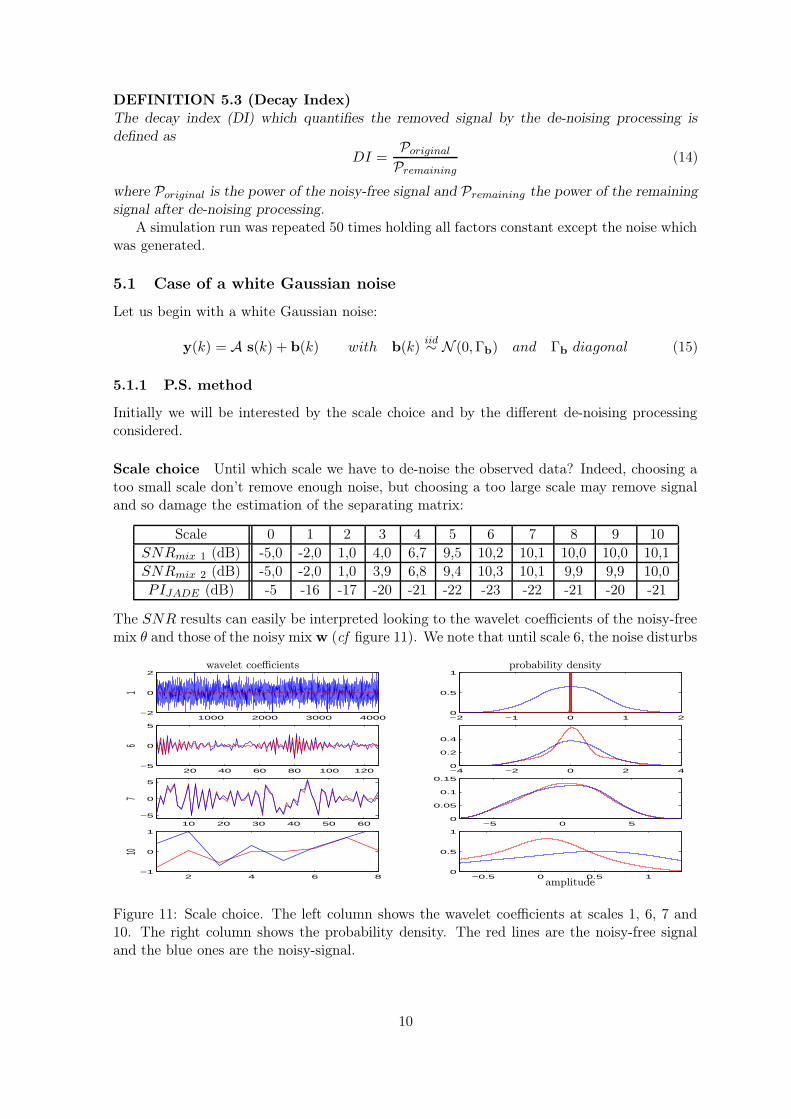
(Figure 13). We note that, after the separation, the remaining signal in the estimated sources

200 400 600 800 1000

−1.5

−1

−0.5

0

0.5

1

1.5

500 1000 1500 2000 2500 3000

−1

−0.5

0

0.5

1

200 400 600 800 1000

−1.5

−1

−0.5

0

0.5

1

1.5

500 1000 1500 2000 2500 3000

−1

−0.5

0

0.5

1

PSfrag replacements

a) b)

c) d)

Figure 13: Remaining signals versus the methods. a) and b) are related to D.P.S.P. and c)and d) are related to P.S. The red lines are the sources and the blue ones the product ofthe remaining signal after the pre-separating de-noising processing by the separating matrixBDmbfy

.

is almost perfect (Fig. 13 a and b). On the other hand, the methods P.S. (Fig. 13 c and d) orP.S.P. don’t give such good results.

5.1.4 Comparison of the methods

Let compare the different methods proposed, using the performance index PI and SNR indB.

SNRe -10 -5 0 5 -10 -5 0 5

without denoisingPIJADE 0 -5 -22 -24 SNR1 -9.2 -5.0 -0.3 4.7PIEASI 1 -2 -15 -24 SNR2 -9.1 -4.5 0.3 5.3

P.S. (6,0)PIJADE -18 -22 -24 -24 SNR1 5.9 9.9 13.8 17.3PIEASI -14 -19 -21 -24 SNR2 5.6 10.1 14.8 19.0

P.S.P. (5,6)PIJADE -17 -21 -23 -24 SNR1 7.4 11.9 15.6 17.8PIEASI -13 -18 -21 -23 SNR2 7.0 11.6 16.6 21.4

D.P.S.P. (6,6 or 5)PIJADE -17 -23 -27 -29 SNR1 8.1 12.5 16.1 18.1PIEASI -14 -18 -22 -24 SNR2 7.8 11.3 16.4 21.4

We note that the P.S.P. and D.P.S.P. improve the performances (cf SNR of the estimatedsources). These two methods have the same behavior if the scale of the pre-separation de-noising is well chosen.

Let us compare those methods when the scale of pre-separation de-noising is over-estimated.The following tabular reports the SNR (dB) and the PI (dB) in the case (9,·).

13

``

``

``

``

``

``

`Method

SNR (dB)-10 dB -5 dB 0 dB 5 dB

without denoisingSNR1 -9,2 -5,0 -0,3 4,7SNR2 -9,1 -4,5 0,3 5,3

PI 0 -5 -22 -24

P.S.P.SNR1 2,7 9,8 14,8 17,5SNR2 2,3 8,3 15,0 21,1

PI 1 -12 -22 -24

D.P.S.P.SNR1 5,5 11,4 15,7 18,0SNR2 4,3 10,8 16,3 21,5

PI 1 -12 -23 -24

We note that D.P.S.P. is less sensitive than P.S.P. Indeed, for D.P.S.P., even if the separatingmatrix is not well estimated, the original signal is used for the post-denoising, while for P.S.P.,if the pre-separation de-noising VERBE too much the signal, it will be impossible to recoverthe sources. D.P.S.P. is then more robust than P.S. or P.S.P.

2000 4000 6000 8000

−1.5

−1

−0.5

0

0.5

1

1.5

2000 4000 6000 8000

−1.5

−1

−0.5

0

0.5

1

1.5

2000 4000 6000 8000

−2

−1

0

1

2

2000 4000 6000 8000

−1.5

−1

−0.5

0

0.5

1

1.5

PSfrag replacements

a) b)

c) d)

Figure 14: Estimated sources in the case (9,·) with SNR mixtures egal to -5dB. The figuresa) and c) are related to P.S.P. and the b) and d) are related to D.P.S.P. The red lines are thesources and the blue ones are the estimated sources.

5.2 Case of a colored Gaussian noise

Until now, we consider a white Gaussian noise, let study the methods with a colored Gaussiannoise. The simulations were performed with short time dependence noise, modeled by an auto-regressive process AR(2):

b(k) = 1.33b(k − 1) − 0.88b(k − 2) + d(k) (16)

with d(k) an iid Gaussian noise. The filtered noise b(k) is no longer iid as shown by the PSDin figure 15b, ie. the noise coefficients are scale-dependent. Thus, we will use a scale-dependentthreshold: σe

√2 lnN , where σ2

e is the variance at scale e estimated using:

σe =1

0, 6745Med(|we|)

14

100 200 300 400 500 600 700 800 900 1000−10

−5

0

5

10

0 0.05 0.1 0.15 0.2 0.25 0.3 0.35 0.4 0.45 0.5

10−2

100

102

PSfrag replacements

samples

frequency

a)

b)

Figure 15: Colored noise: a) the colored noise b(k), b) the power spectral density.

where we are the noisy wavelet coefficients at scale e and Med(|x|) is the median of theabsolute values of the vector x components.

In this case, we only report the PI and the SNR of the estimated sources. Based onthe previous discussion the scale of the pre-separation de-noising is equal to 5, and the scalesof the post-separation de-noising, are equal to 5 and 6 for the first and the second sources,respectively.

The hard threshold of the stationnary wavelet transform is very effective (cf PI).

SNRe -10 -5 0 5 -10 -5 0 5

without denoisingPIJADE 0 -1 -15 -23 SNR1 -9,3 -4,7 -0,3 4,7PIEASI 0 -2 -12 -21 SNR2 -9 -4,4 0,3 5,3

P.S. (SURE)PIJADE -10 -22 -24 -24 SNR1 7,2 11,6 16,0 19,0PIEASI -14 -19 -23 -24 SNR2 7,9 12,8 17,4 21,5

P.S.P. (5,6) and(5,5)

PIJADE -21 -23 -24 -24 SNR1 11,2 14,9 17,6 19,6PIEASI -18 -20 -23 -24 SNR2 10,6 14,8 20,0 25,0

D.P.S.P. (6,6) and(6,5)

PIJADE -22 -24 -24 -25 SNR1 11,8 15,3 17,5 19,7PIEASI -19 -21 -23 -24 SNR2 10,3 14,9 20,0 24,9

This tabular illustrates the interest of a post-separation de-noising. If the scales are wellchoosen, the methods P.S.P. and D.P.S.P. still improve the performance.

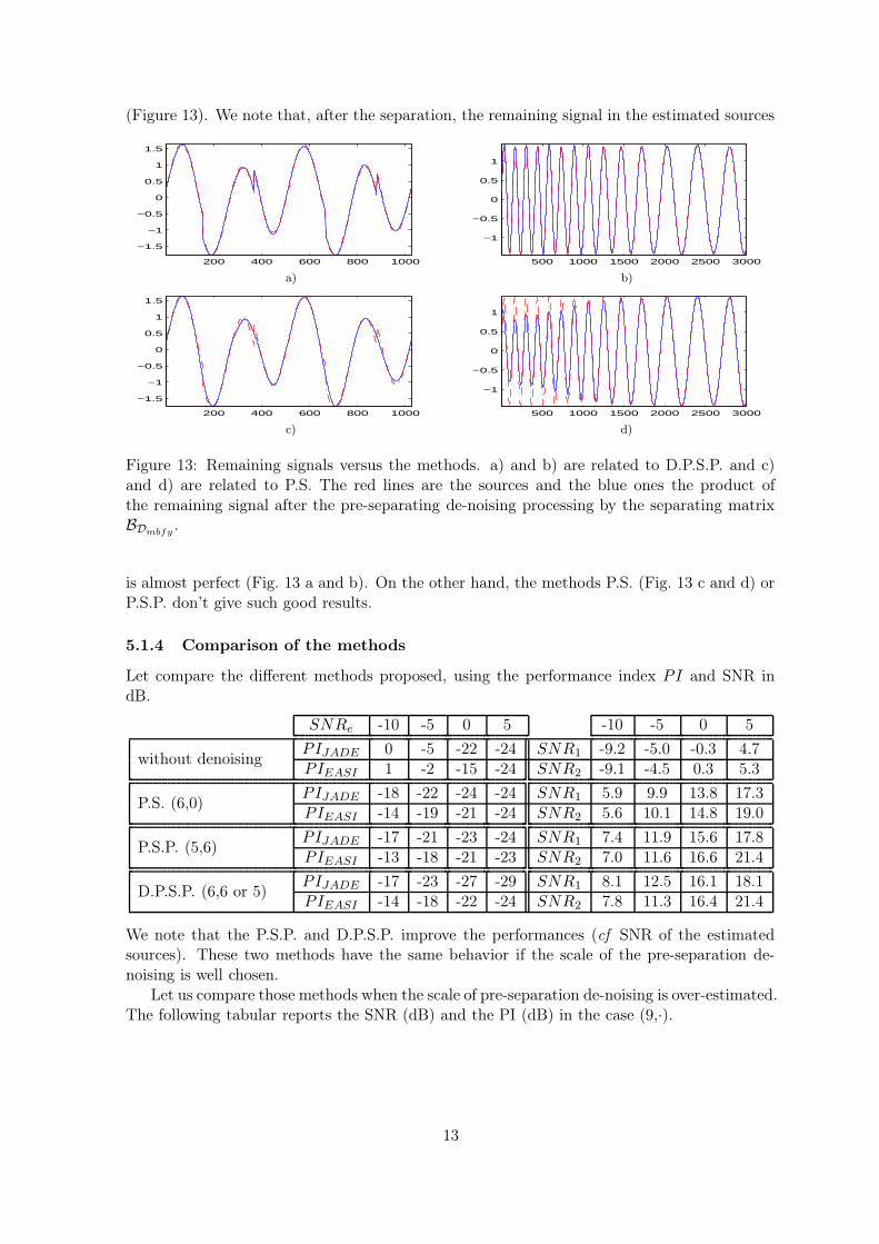
Let study now the results if the scale of the pre-separation de-noising is over-estimated.In the next table, the scale of the pre-separation de-noising is equal to 7 (the separatingalgorithm is JADE).

15

``

``

``

``

``

``

`Method

SNR (dB)-10 dB -5 dB 0 dB 5 dB

without denoisingSNR1 -9,3 -4,7 -0,3 4,7SNR2 -9,0 -4,4 0,3 5,3

PI 0 -1 -15 -23

P.S. (SURE)SNR1 1,2 1,1 2,7 2,9SNR2 2,2 2,1 2,6 2,8

PI 2 1 -8 -14

P.S.P.SNR1 5,1 5,5 5,7 5,8SNR2 2,4 2,6 2,6 2,7

PI -5 -9 -10 -12

D.P.S.P.SNR1 10,7 13,9 15,5 16,2SNR2 9,0 12,8 15,2 16,5

PI -5 -9 -10 -12

We note that the D.P.S.P. is still more robust than the others methods. This can be explainedby the estimation of the variance of the noise. Indeed, σe is estimated by the median, whichsupposes that more half of the coefficients which are higher than the median are due to thenoise. But at large scales, the coefficients due to the signal become large which increasesartificially the threshold. In this case, an over-estimated value of the scale turns out to becatastrophic except for the D.P.S.P.

6 Fetal ECG extraction

In the previous section, we have introduced many solutions for associating wavelet de-noisingand blind source separation. We will now apply these methods to the fetal ECG extraction.

6.1 Observed data

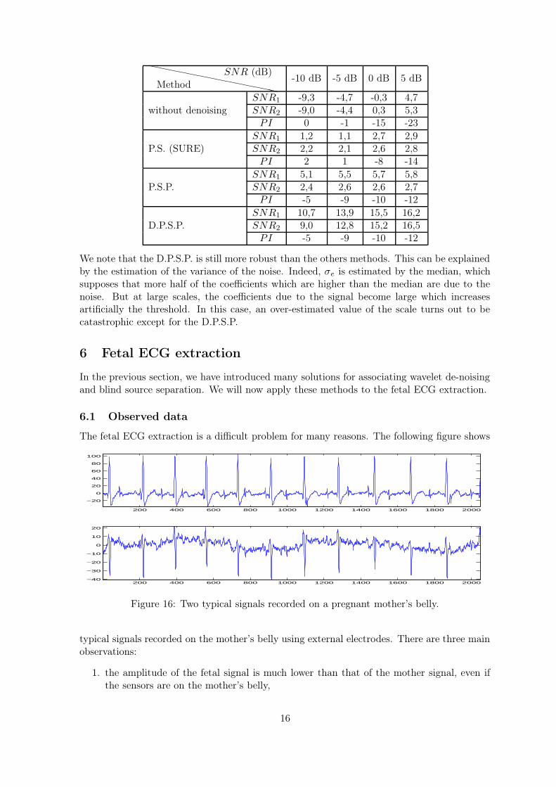
The fetal ECG extraction is a difficult problem for many reasons. The following figure shows

200 400 600 800 1000 1200 1400 1600 1800 2000

−20

0

20

40

60

80

100

200 400 600 800 1000 1200 1400 1600 1800 2000−40

−30

−20

−10

0

10

20

Figure 16: Two typical signals recorded on a pregnant mother’s belly.

typical signals recorded on the mother’s belly using external electrodes. There are three mainobservations:

1. the amplitude of the fetal signal is much lower than that of the mother signal, even ifthe sensors are on the mother’s belly,

16

2. the heartbeat rate of the foetus is about twice faster than the mother’s one, which canbe explained by its smaller size,

3. in the second signal (Fig. 16 bottom), noise and fetal ECG have about the same power.

6.2 Fetal ECG extraction from simulated signals

In the first time, we will test the wavelet de-noising processing and blind source separationon artificial ECGs generated by a simulator. This simulator [12] allows us to adjust theheartbeat rate of the mother ECG as well as the heartbeat rate and amplitude of the fetalECG. We could optionally add other sources as uterus and diaphragm electrical activity. Inour simulations only fetal and mother ECG are present.

6.3 Noisy-free data

The following figure shows artificial noisy-free data and estimated sources. The attribution

0 500 1000 1500−2

−1

0

1

0 500 1000 1500−3

−2

−1

0

1

0 500 1000 1500−6

−4

−2

0

2

0 500 1000 1500−4

−2

0

2

0 500 1000 1500−1

−0.5

0

0.5

1

0 500 1000 1500−2

−1

0

1

PSfrag replacements

a)

d)

b)

e)

c)

f)

0 500 1000 1500−5

0

5

10

0 500 1000 1500−10

−5

0

5

0 500 1000 1500−10

−5

0

5

0 500 1000 1500−10

−5

0

5

0 500 1000 1500−5

0

5

0 500 1000 1500−5

0

5

PSfrag replacements

a) d)

b) e)

c) f)

Figure 17: Estimated sources from artificial noisy-free mixtures. The six left plots are relatedto the six mixtures and the six right plots are related to the estimated sources. a), b) and c)are related to the mother’s heart and d), e) and f) to the fetal heart.

with the mother or the foetus of the sources is done by considerations on the rate of theheartbeat. In this condition, the algorithm JADE separates the different sources.

6.4 Noisy data

Now, the observed data have a SNR equal to 10dB compared to the fetal signal, i.e. SNR =Pfetal/Pnoise = 10dB. In this case, source separation partily fails: the signals of the motherare well estimated but those of the foetus are lost in a large noise (Figures 18 and 19).

In order to understand what happens, we consider the term B n (see equation 2). Then,the output SNR can be very bad, depending of the separating matrix B, ie. of the mixingmatrix A since B = A−1. To show that, we will consider the academic example of two sourcess1 and s2 mixed by the following mixing matrix

A =

(

1 0−1 1

)

17

0 500 1000 1500−2

−1

0

1

0 500 1000 1500−3

−2

−1

0

1

0 500 1000 1500−6

−4

−2

0

2

0 500 1000 1500−4

−2

0

2

0 500 1000 1500−1

−0.5

0

0.5

1

0 500 1000 1500−2

−1

0

1

PSfrag replacements

a)

d)

b)

e)

c)

f)

0 500 1000 1500−5

0

5

10

0 500 1000 1500−5

0

5

10

0 500 1000 1500−10

−5

0

5

0 500 1000 1500−5

0

5

10

0 500 1000 1500−5

0

5

0 500 1000 1500−5

0

5

PSfrag replacementsa) d)

b) e)

c) f)

Figure 18: Estimated sources from artificial noisy mixtures. The six left plots are related tothe six mixtures and the six right plots are related to the estimated sources. a), b) and c) arerelated to the mother’s heart and d), e) and f) to the fetal heart.

0 500 1000 1500−10

−5

0

5

0 500 1000 1500−5

0

5

0 500 1000 1500−10

−5

0

5

0 500 1000 1500−5

0

5

10

0 500 1000 1500−5

0

5

0 500 1000 1500−5

0

5

PSfrag replacements

a) d)

b) e)

c) f)

g)

h)

i)

j)

k)

l)

Figure 19: Noisy data provides noisy estimated sources. The red lines are related to the idealsources and the blue ones are related to the term Bn. a), b) and c) are related to the mother’sheart and d), e) and f) to the fetal heart

The two eigen values are equal to 1, thus the matrix is well conditioned and its inverse isequal to

B =

(

1 01 1

)

Thus, with a Gaussian noise of variance σ2, the SNR of the second source is divided by 2compared with the mixtures SNR. So, in order to obtain a high output SNR it seems to benecessary that there are, on a row of the separating matrix B, only one coefficient of largevalue, which occurs the mixing matrix is almost diagonal.

In other words, in the fetal ECG extraction context, the location of the sensors is veryimportant.

6.5 Pre-processing from real data

When the heart is not stimulated, the theorical ECGs should present a horizontal base line(Figure 20). However, on experimental ECGs, the base line is not iso-electrical due to bad

18

1 2 3 4 5 6 7 8 9

−6

−5

−4

−3

−2

−1

0

1

2

3

4

PSfrag replacements

temps

Figure 20: Example of removing base line. The red line is the blue line without the base lineremoved by the proposede algorithm.

contacts between the sensor and the skin, or to the breathing, etc. In order to remove thisbase line, if its frequency is lower than the rate (which often holds) we propose the followingmethod. The signal is decomposed by wavelets until the scale which fits with the rate of theheartbeat and a new signal is constructed by inverse transformation where the coefficientsof the approximation are enforced to zero (Figure 20). In order to justify the shape of thespectrum of the ECG, we have modelized it (Figure 21): the different waves are estimated

1000 2000 3000 4000 5000

0

1

2

3

4

100 200 300 400

0

1

2

3

4

0 0.01 0.02 0.03 0.04 0.05 0.06 0.07 0.08 0.09 0.10

0.05

0.1

0.15PSfrag replacements

samplessamples

a) b)

c)

frequency

Figure 21: A frequency study of the ECG. a) a serie of heartbeats, b) a single heartbeat andc) the spectrum of respectively (red curve) the single heartbeat and (blue curve) the serie ofheartbeats.

by triangles where Fourrier transform is a square cardinal sine wave which explains the wayof a heartbeat. Let study now the way of a set of heartbeats. In the temporal space, thesignal can be estimated by the convolution of a heartbeat and a Dirac comb (period equal toTRR: interval between two R waves). So the Fourrier transform is the product of the Fourriertransform of a heartbeat and a Dirac comb with a period equal to 1/TRR which explains thediscret spectrum: the spectrum of a serie of hearbeats is a Dirac comb modulated by theheartbeat spectrum.

Moreover, we propose to adapt the sample frequency Fe to the ECG spectrum: to choose

19

a Shannon frequency (Fe/2) equal at twice the maximum frequency Fm in the ECG seems tobe a good compromise between the SNR (which supposes the lowest sample frequency) andthe power of the noise (which supposes a larger sample frequency).

7 Conclusion

The fetal ECG extraction from sensors located on the mother’s skin is a hard problem.Broached with classical methods, the results are bad [13]. The reformulation of the problemas blind source separation problem by De Lathauwer [14] gives promising results. However,the noise strongly limits the performance encouraging us to use wavelet de-noising processing.In this paper, we propose two new principles, P.S.P. and D.P.S.P., which associate waveletde-noising and blind source separation. These principles improve the performances of theseparation. Moreover the D.P.S.P. is more robust to a bad pre-separation de-noising withwhite as well as colored Gaussian noise.

References

[1] J. Hérault, C. Jutten, and B. Ans. Détection de grandeurs primitives dans un messagecomposite par une architecture de calcul neuromimétrique en apprentissage non supervisé.In Gretsi, volume 2, pages 1017–1020, Nice, mai 1985.

[2] C. Jutten and A. Taleb. Source separation: from dusk till dawn. In Independent

compoment analysis 2000, pages 15–26, Helsinki, Finlande, June 2000.

[3] S. Amari and A. Cichocki. Adaptive Blind Signal and Image Processing, Learning

Algorithms and Applications. Wiley, 2002.

[4] A. Hyvärinen, J. Karhunen, and E. Oja. Independent Component Analysis. Wiley,2001.

[5] S. Mallat. A wavelet tour of signal processing. Academic Press, second edition, 1999.

[6] I. Cohen, S. Raz, and D. Mallat. Orthonormal shift-invariant wavelet packet decom-position and representation. Signal Processing, vol. 57(1):pp. 251–270, 1997.

[7] G. P. Nason and B. W. Silverman. The stationary wavelet transform and some statis-tical applications. Technical report, University of Bristol, February 1995.

[8] A. Paraschiv-Ionescu, C. Jutten, K. Aminian, and al. Source separation in strongnoisy mixtures: a study of wavelet de-noising pre-processing. In ICASSP’2002, Orlando,Floride, 2002.

[9] H.H. Yang, S. Amari, and A. Cichocki. Information-theoric approach to blind sepa-ration of sources in non-linear mixture. Signal Processing, 64(3):291–300, February 1998.

[10] J.F. Cardoso. Multidimensional independent component analysis. In Proc. ICASSP’98,pages 1941–1944, 1998.

[11] J.F. Cardoso and B.H. Laheld. Equivariant adaptive source separation. IEEE Trans.

Signal Processing, 44(12):3017–3030, December 1996.

[12] M. Schmidt. Sensor array for fetal ecg signals simulation, sensor selection and sourceseparation. Technical report, Laboratoire des Images et des Signaux, Grenoble, France,2003.

20

[13] Vicente Zarzoso and Asoke K. Nandi. Noninvasive fetal electrocardiogram extrac-tion: blind source separation versus adaptative noise cancellation. IEEE Transactions on

Biomedical Engineering, vol. 48(1):pp. 12–18, January 2001.

[14] L. De Lathauwer, D .Callaerts, B. De Moor, and al. Fetal electrocardiogramextraction by source subspace separation. In Proc. IEEE Workshop on HOS, pages 134–138, Girona, Spain, June 12–14 1995.

21