NN

T:2

018S

AC

LA04

2

Uncertainty quantification and calibrationof a photovoltaic plant model: warranty ofperformance and robust estimation of the

long-term productionThese de doctorat de l’Universite Paris-Saclay

preparee a AgroParisTech (l’Institut des sciences et industries du vivant et del’environnement)

Ecole doctorale n581 Agriculture, Alimentation, Biologie, Environnement,Sante (ABIES)

Specialite de doctorat : Mathematiques appliquees

These presentee et soutenue a Paris, le 21 Decembre 2018, par

MATHIEU CARMASSI

Composition du Jury :

Liliane BelProfesseur, AgroParisTech (MIA Paris) PresidentAmandine MarrelIngenieur-Chercheur, CEA Cadarache (DER/SESI) RapporteurOlivier RoustantProfesseur, Ecole des Mines de Saint-Etienne (LIMOS) RapporteurLuc PronzatoDirecteur de Recherche, CNRS (I3S) ExaminateurEric ParentIGPEF, AgroParisTech (MIA Paris) Directeur de thesePierre BarbillonMaıtre de Conference, AgroParisTech (MIA Paris) Co-directeur de theseMatthieu ChiodettiIngenieur, EDF (TREE) Co-encadrantMerlin KellerIngenieur-Chercheur, EDF (PRISME) Invite

REMERCIEMENTS

Je voudrais avant tout remercier mon directeur de thèse Éric Parent pour m’avoir guidé durant ces trois années dethèse. Ses qualités scientifiques et humaines ont contribué au très bon déroulement de cette thèse. Éric a su trouverun bon équilibre dans l’encadrement, en étant très présent au début lorsque le besoin s’en ressentait et en me laissantune certaine marge de manœuvre par la suite. Je tiens à souligner sa constante bonne humeur et son côté paternelqui m’a soulagé de la pression lorsque celle-ci se faisait trop importante.

Ensuite, je tiens à remercier mon co-directeur de thèse Pierre Barbillon pour m’avoir aiguillé scientifiquementdurant ces trois années. J’ai pu bénéficier de ses grandes qualités scientifiques à n’importe quel moment et leséchanges que nous avons eus se sont toujours révélés très productifs. Son perfectionnisme m’a aussi amené à nerien négliger que ce soit au niveau rédactionnel ou scientifique. J’ai pu apprécier sa personnalité au quotidien, quece soit pendant les soirées à Rochebrune, pendant les réunions de travail ou pendant les pauses-café dans le bureaudes doctorants. Une chose est sûre c’est que les jeux de mots quasi quotidiens vont me manquer.

Je tiens aussi à adresser mes remerciements à Merlin Keller. Il est indéniablement la raison pour laquellej’ai pu en arriver là. Sa constante bonne humeur, sa modestie et ses qualités scientifiques ont été la source d’unecollaboration qui dure depuis mon stage de fin d’année d’école d’ingénieurs. J’ai pu le solliciter autant de fois queje le souhaitais pendant la thèse et même si je ne travaillais pas sur le même site, il a toujours été là pour m’aider. Àchaque réunion que nous avons eue, j’ai pu retrouver chez lui un juste recul sur les problèmes industriels avec unegrande connaissance mathématique.

Je remercie également Amy Lindsay qui m’a encadré avec une grande qualité jusqu’à sa mutation qui estintervenue au bout d’un an de thèse. C’est aussi pour cela que je remercie grandement Matthieu Chiodetti qui s’estretrouvé avec ma thèse sur les bras. Son encadrement a été d’une très grande qualité et il a su m’orienter sur lesbesoins industriels précis d’EDF et son expertise dans le domaine m’a permis de prendre du recul sur les résultatsque l’on pouvait avoir. De manière générale, j’ai pu tisser avec chacun des membres de mon encadrement des liensd’amitié qui se sont retranscrit dans des conférences ou écoles d’été (Rochebrune, ETICS,...) où nous étions parfoisamenés à sortir du cadre professionnel.

J’adresse également mes remerciements à Amandine Marrel et Olivier Roustant pour avoir accepté de rapporterma thèse. Le travail sur les rapports a grandement été apprécié. Je remercie aussi Liliane Bel d’avoir présidé masoutenance de thèse et Luc Pronzato d’avoir accepté de faire partie de mon jury en tant qu’examinateur.

Mes prochains remerciements seront pour mes collègues d’EDF. Même si le site des Renardières se trouvait trèsloin de mon domicile, c’était toujours avec un grand plaisir que je retrouvais tout le groupe. J’ai toujours appréciéles échanges, à table ou pendant les pauses, que nous avons eu. Je remercie tout particulièrement mon laboratoireMIA d’AgroParisTech qui m’a apporté énormément durant cette thèse. Au-delà des compétences mathématiquesdont j’ai pu bénéficier, j’ai pu tisser des liens d’amitiés forts avec d’autres doctorants. Merci Timothée, Marie P,Pierre G (déjà vieux docteur), Félix, Rana, Paul, Anna, Marie C, Loïc d’avoir animé, à un moment ou un autre, lebureau des doctorants. Les afterworks à la Montagne, au Vieux Chêne, ou dans la rue Mouffetard nous ont permisde décompresser avec des journées de travail bien chargées.

3

Je tiens bien entendu à remercier toute ma famille : ma mère Marie-Christine, mon père Patrick, mon frèreGuillaume et ma grand-mère Jeanine. Je pense sincèrement que le cadre familial qu’ils ont établi m’a conduit là oùje suis aujourd’hui et je n’aurais pas pu rêver d’un meilleur équilibre de vie.

Je tiens désormais à remercier tous mes amis qui m’ont épaulé de près ou de loin pendant la thèse. D’abord,je remercie Quentin Huchet qui a été dans la même galère que moi et avec qui j’ai partagé quelques écoles d’étéqui sont devenues mythiques (Porquerolles, Roscoff, ...). Merci de m’avoir permis de rigoler profondément à desmoments où j’en avais besoin, d’avoir tourné en dérision les situations compliquées, d’avoir toujours eu le motmarrant pour dédramatiser le contexte. Merci à Lambert pour les pauses printemps de Bourges ou pour les quelquesweek-ends pétanque, hors du temps, à Paris. Merci à Albin pour les pauses rugby au bar ou les brainstormingsnon fructueux qui se terminaient quasi systématiquement en bières/rugby. Je remercie toute la clique de l’IFMA: Tareck, Pilou, Vely, Alexia, ViVi, MiMi, Norman, Naf, Matthieu, Ludo pour les week-ends de retrouvailles oules réveillons du nouvel an passés ensemble. C’était aussi agréable de se retrouver des soirs aux Lombards, MacBride, Halls Beer, et autres tavernes. Les moments pendant la coupe du monde sur cette petite place pleine à craquerresteront aussi des moments marquants.

La conclusion de ces remerciements ne peut concerner que la personne qui m’a épaulé durant ces trois dernièresannées. Je remercie Camille pour m’avoir soutenu et supporté comme elle l’a fait même dans les moments où jedevenais insupportable. Merci de m’avoir poussé à faire des breaks qui m’ont permis de mieux repartir après. Mercipour ces voyages qui n’appartiennent qu’à nous et qui m’ont permis de m’évader le temps de quelques semaines.Merci de ne m’avoir jamais laissé tomber au fond du trou et de m’avoir poussé à repartir rapidement après. Mercipour ta joie de vivre et ta constante foi en moi qui me redonnait confiance dans les mauvais moments. Merci d’avoirrendu cette thèse plus facile.

4

CONTENTS

Remerciements 3

List of figures 9

Acronyms 11

Résumé 13

1 Introduction 191.1 Economic issue . . . . . . . . . . . . . . . . . . . . . . . . . . . . . . . . . . . . . . . . . . . . 19

1.2 Physical phenomenon . . . . . . . . . . . . . . . . . . . . . . . . . . . . . . . . . . . . . . . . . 21

1.3 Several modeling approaches . . . . . . . . . . . . . . . . . . . . . . . . . . . . . . . . . . . . 22

1.3.1 A first simple model . . . . . . . . . . . . . . . . . . . . . . . . . . . . . . . . . . . . . 22

1.3.2 Advanced electrical models . . . . . . . . . . . . . . . . . . . . . . . . . . . . . . . . . 23

1.4 Numerical codes . . . . . . . . . . . . . . . . . . . . . . . . . . . . . . . . . . . . . . . . . . . 25

1.4.1 General framework . . . . . . . . . . . . . . . . . . . . . . . . . . . . . . . . . . . . . . 25

1.4.2 Sources of uncertainties . . . . . . . . . . . . . . . . . . . . . . . . . . . . . . . . . . . 25

1.4.3 Python code . . . . . . . . . . . . . . . . . . . . . . . . . . . . . . . . . . . . . . . . . . 26

1.4.4 Dymola code . . . . . . . . . . . . . . . . . . . . . . . . . . . . . . . . . . . . . . . . . 27

1.5 Thesis organization . . . . . . . . . . . . . . . . . . . . . . . . . . . . . . . . . . . . . . . . . . 30

2 Statistical tools for numerical code calibration 312.1 Sensitivity analysis . . . . . . . . . . . . . . . . . . . . . . . . . . . . . . . . . . . . . . . . . . 33

2.1.1 Morris method . . . . . . . . . . . . . . . . . . . . . . . . . . . . . . . . . . . . . . . . 33

2.1.2 Sobol indices . . . . . . . . . . . . . . . . . . . . . . . . . . . . . . . . . . . . . . . . . 39

2.2 Kriging / Gaussian processes . . . . . . . . . . . . . . . . . . . . . . . . . . . . . . . . . . . . . 42

2.2.1 General framework . . . . . . . . . . . . . . . . . . . . . . . . . . . . . . . . . . . . . . 42

2.2.2 Parameter estimation . . . . . . . . . . . . . . . . . . . . . . . . . . . . . . . . . . . . . 45

2.2.3 Covariance functions . . . . . . . . . . . . . . . . . . . . . . . . . . . . . . . . . . . . . 47

2.2.4 Gaussian process-based optimization . . . . . . . . . . . . . . . . . . . . . . . . . . . . 48

2.3 Design of experiments . . . . . . . . . . . . . . . . . . . . . . . . . . . . . . . . . . . . . . . . 51

2.3.1 Sampling criteria . . . . . . . . . . . . . . . . . . . . . . . . . . . . . . . . . . . . . . . 51

2.3.2 Distance between the points criteria . . . . . . . . . . . . . . . . . . . . . . . . . . . . . 52

2.4 Principal component analysis (PCA) . . . . . . . . . . . . . . . . . . . . . . . . . . . . . . . . . 54

2.4.1 Distance . . . . . . . . . . . . . . . . . . . . . . . . . . . . . . . . . . . . . . . . . . . . 54

2.4.2 Moments of inertia . . . . . . . . . . . . . . . . . . . . . . . . . . . . . . . . . . . . . . 55

2.4.3 Axis of minimum inertia . . . . . . . . . . . . . . . . . . . . . . . . . . . . . . . . . . . 56

2.4.4 Contribution to the total inertia . . . . . . . . . . . . . . . . . . . . . . . . . . . . . . . . 58

2.4.5 Graphical representations . . . . . . . . . . . . . . . . . . . . . . . . . . . . . . . . . . . 58

2.5 Monte Carlo Markov Chains techniques . . . . . . . . . . . . . . . . . . . . . . . . . . . . . . . 61

2.5.1 Gibbs sampler . . . . . . . . . . . . . . . . . . . . . . . . . . . . . . . . . . . . . . . . 62

5

CONTENTS

2.5.2 Metropolis Hastings . . . . . . . . . . . . . . . . . . . . . . . . . . . . . . . . . . . . . 632.5.3 Metropolis within Gibbs . . . . . . . . . . . . . . . . . . . . . . . . . . . . . . . . . . . 652.5.4 Improvements of the Metropolis Hastings . . . . . . . . . . . . . . . . . . . . . . . . . . 65

3 Review of the main calibration methods 693.1 Numerical code . . . . . . . . . . . . . . . . . . . . . . . . . . . . . . . . . . . . . . . . . . . . 70

3.1.1 Sensitivity analysis . . . . . . . . . . . . . . . . . . . . . . . . . . . . . . . . . . . . . . 703.1.2 Prior propagation of uncertainty . . . . . . . . . . . . . . . . . . . . . . . . . . . . . . . 72

3.2 Calibration through statistical models . . . . . . . . . . . . . . . . . . . . . . . . . . . . . . . . 733.2.1 Presentation of the models . . . . . . . . . . . . . . . . . . . . . . . . . . . . . . . . . . 743.2.2 Likelihood . . . . . . . . . . . . . . . . . . . . . . . . . . . . . . . . . . . . . . . . . . 763.2.3 Estimation . . . . . . . . . . . . . . . . . . . . . . . . . . . . . . . . . . . . . . . . . . 80

3.3 Application to the prediction of power from a photovoltaic (PV) plant . . . . . . . . . . . . . . . 823.3.1 Inference . . . . . . . . . . . . . . . . . . . . . . . . . . . . . . . . . . . . . . . . . . . 823.3.2 Results . . . . . . . . . . . . . . . . . . . . . . . . . . . . . . . . . . . . . . . . . . . . 853.3.3 Comparison . . . . . . . . . . . . . . . . . . . . . . . . . . . . . . . . . . . . . . . . . . 87

3.4 Conclusion and discussion . . . . . . . . . . . . . . . . . . . . . . . . . . . . . . . . . . . . . . 88

4 CaliCo: a R package for Bayesian calibration 914.1 Guidelines for users . . . . . . . . . . . . . . . . . . . . . . . . . . . . . . . . . . . . . . . . . . 924.2 Multidimensional example with CaliCo . . . . . . . . . . . . . . . . . . . . . . . . . . . . . . . 97

4.2.1 The models . . . . . . . . . . . . . . . . . . . . . . . . . . . . . . . . . . . . . . . . . . 984.2.2 Priors . . . . . . . . . . . . . . . . . . . . . . . . . . . . . . . . . . . . . . . . . . . . . 1024.2.3 Calibration . . . . . . . . . . . . . . . . . . . . . . . . . . . . . . . . . . . . . . . . . . 1034.2.4 Additionnal tools . . . . . . . . . . . . . . . . . . . . . . . . . . . . . . . . . . . . . . . 108

4.3 Conclusion . . . . . . . . . . . . . . . . . . . . . . . . . . . . . . . . . . . . . . . . . . . . . . 111

5 Performance monitoring on a large PV plant 1135.1 Sensitivity analysis . . . . . . . . . . . . . . . . . . . . . . . . . . . . . . . . . . . . . . . . . . 1135.2 Prior densities . . . . . . . . . . . . . . . . . . . . . . . . . . . . . . . . . . . . . . . . . . . . . 1175.3 Propagation of uncertainties . . . . . . . . . . . . . . . . . . . . . . . . . . . . . . . . . . . . . 1185.4 Bayesian calibration . . . . . . . . . . . . . . . . . . . . . . . . . . . . . . . . . . . . . . . . . . 118

5.4.1 Statistical models . . . . . . . . . . . . . . . . . . . . . . . . . . . . . . . . . . . . . . . 1185.4.2 Modular estimation and likelihoods . . . . . . . . . . . . . . . . . . . . . . . . . . . . . 1205.4.3 Application to the PV plant . . . . . . . . . . . . . . . . . . . . . . . . . . . . . . . . . 121

6 Conclusion and perspectives 129

Bibliography 136

6

LIST OF FIGURES

1.1 p-n junction and the equivalent electrical component (source: Raffamaiden – CC By SA). . . . . . 21

1.2 n side doping. . . . . . . . . . . . . . . . . . . . . . . . . . . . . . . . . . . . . . . . . . . . . . 21

1.3 p side doping. . . . . . . . . . . . . . . . . . . . . . . . . . . . . . . . . . . . . . . . . . . . . . 21

1.4 Displacement of an electron in the silicon (source: Freshman404 – CC By SA). . . . . . . . . . . 22

1.5 On the left panel, the electrical equivalence with 1 diode where IPV stands for a photo-current thatdepends on the incident sun rays, ID for the saturation current of the ideal diode, RP the shuntresistance, RS the series resistance representing losses proportional to I, I the current and V thevoltage generated by the cell. On the right panel the electrical equivalence with 2 diodes where ID1

and ID2 stands for the saturation current of both ideal diodes. . . . . . . . . . . . . . . . . . . . . 23

1.6 I/V curve of a toy example. . . . . . . . . . . . . . . . . . . . . . . . . . . . . . . . . . . . . . . 24

1.7 The power production by PVzen for August 2014 (on the left) and the power production averagedby hour for August 25th 2014 (on the right). . . . . . . . . . . . . . . . . . . . . . . . . . . . . . 27

1.8 On the top left, the original scaled power production gathered on the the PV plant during the year2015. On the top, right the same data but only on the first week. On the bottom left, the originaldata but averaged by hour. On the bottom right, only the positive power is kept among the origin data. 29

2.1 Major steps in uncertainty treatment for industrial matters (source: Bertrand Iooss – ENBIS-EMSE

2009 Conference). . . . . . . . . . . . . . . . . . . . . . . . . . . . . . . . . . . . . . . . . . . . 32

2.2 Sampling grid on the scaled space. . . . . . . . . . . . . . . . . . . . . . . . . . . . . . . . . . . 34

2.3 On the left panel a result of Morris method on the Morris function and on the right panel 10repetitions of the method. . . . . . . . . . . . . . . . . . . . . . . . . . . . . . . . . . . . . . . . 37

2.4 Scatter plot of the Morris indices given by the 1500 iterations bootstrap. . . . . . . . . . . . . . . 39

2.5 Scatter plots of the Ishigami function where the output is given function of the each parameter. . . 41

2.6 Sobol’s index computed for the Ishigami function and the boxplots representing the variability of1000 bootstrap iterations. . . . . . . . . . . . . . . . . . . . . . . . . . . . . . . . . . . . . . . . 41

2.7 Different Gaussian process emulations for the toy function defined Equation (2.30). On the firstpanel (on the left) the Gaussian process is estimated with σ2 = 1 and ψ = 0.1. On the second panel(on the middled left), σ2 = 5 and ψ = 0.1. On the third panel (on the middle right), σ2 = 1 andψ = 0.2. And, on the fourth panel (on the right), σ2 = 5 and ψ = 0.2. . . . . . . . . . . . . . . . 44

2.8 Different Gaussian process estimation for the toy function Equation (2.30) with σ2 = 5 and ψ = 0.1but with different covariance functions. On the first panel (on the left) the Gaussian process isestimated with Gaussian covariance function. On the second panel (on the middled left), with aMatérn 5/2. On the third panel (on the middle right), with a Matérn 3/2. And, on the fourth panel(on the right), with an exponential. . . . . . . . . . . . . . . . . . . . . . . . . . . . . . . . . . . 47

2.9 Expected improvement computed for the Gaussian process established on the function definedEquation (2.30) with 5 points in the original design of experiments. . . . . . . . . . . . . . . . . . 49

2.10 2 EGO iterations with on top the GP updated based on the previous point found with the EI criterionand on the bottom the EI values corresponding to the GP on top. The point in orange is the EImaximum used to establish the following GP. . . . . . . . . . . . . . . . . . . . . . . . . . . . . 50

7

LIST OF FIGURES

2.11 2 last of the 6 iterations of the EGO algorithm. . . . . . . . . . . . . . . . . . . . . . . . . . . . . 50

2.12 6 points sampled with a LHS for Q = [0,1]2. . . . . . . . . . . . . . . . . . . . . . . . . . . . . 52

2.13 6 points sampled with a LHS for Q = [0,1]2. . . . . . . . . . . . . . . . . . . . . . . . . . . . . 52

2.14 2 6-sized maximin LHS performed with the algorithm of Morris and Mitchell (1995) for 2 parameters. 53

2.15 Graphical representation of the individuals (on the left) and the variables (on the right) of thedecathlon data set. . . . . . . . . . . . . . . . . . . . . . . . . . . . . . . . . . . . . . . . . . . . 60

2.16 Gibbs sampler completed for 10000 iteration with a 1000 burn-in sample. . . . . . . . . . . . . . 63

3.1 On the left panel Morris method at noon the 24th of September 2014 and all the EEs computed ateach time step over the two months of data. . . . . . . . . . . . . . . . . . . . . . . . . . . . . . 70

3.2 Results of the PCA done on the trajectories of the Morris DOE. On the right panel the correlationcircle and on the right panel the eigenvalues. . . . . . . . . . . . . . . . . . . . . . . . . . . . . . 71

3.3 Projection on the PCA axis of the Morris indices. . . . . . . . . . . . . . . . . . . . . . . . . . . 71

3.4 Sobol method completed for each time steps. On the left panel the first order indices and on theright panel the total effects indices. . . . . . . . . . . . . . . . . . . . . . . . . . . . . . . . . . . 72

3.5 π(η), π(µt) and π(ar) prior densities (represented on the left panel) and induced credibility intervalof the instantaneous power (right panel). . . . . . . . . . . . . . . . . . . . . . . . . . . . . . . . 73

3.6 Directed Acyclic Graph (DAG) representation of the different models. . . . . . . . . . . . . . . . 76

3.7 Prior (in blue) and posterior (in red) densities of η , µt , ar and σ2err for each model. On the two first

column the two first models (without and with surrogate) which have only these four parameters toestimate. The two other columns represent the third and the fourth models which have two moreparameters to estimate (see Figure 3.9). . . . . . . . . . . . . . . . . . . . . . . . . . . . . . . . 85

3.8 Correlation representation between the parameters. . . . . . . . . . . . . . . . . . . . . . . . . . 86

3.9 Prior (in blue) and posterior (in red) densities of σ2δ

and ψδ for M3 and M4. . . . . . . . . . . . 86

3.10 Calibration results for M2 and M4 that are using Gaussian processes build on a DOE extended bythe sequential design. . . . . . . . . . . . . . . . . . . . . . . . . . . . . . . . . . . . . . . . . . 88

4.1 Displacement of the oscillator simulated. . . . . . . . . . . . . . . . . . . . . . . . . . . . . . . . 97

4.2 Experimental data displayed when no parameter values are set in the model. . . . . . . . . . . . . 99

4.3 First and second model output for prior belief on parameter values. The left panel illustrates thefirst model and the right panel the second model with the Gaussian process estimated. . . . . . . . 101

4.4 Third and fourth model output for prior belief on parameter values. The left panel illustrates thethird model and the right one, the fourth model with the Gaussian process estimated. Both areencompassing the discrepancy. . . . . . . . . . . . . . . . . . . . . . . . . . . . . . . . . . . . . 102

4.5 M4 displayed for some guessed values with the CI relative to the measurement error on the leftpanel, with the CI relative to the Gaussian process only on the middle panel and both credibilityintervals on the right panel. . . . . . . . . . . . . . . . . . . . . . . . . . . . . . . . . . . . . . . 102

4.6 Prior distributions for each parameter to calibrate in the application case. . . . . . . . . . . . . . . 103

4.7 Series of plot generated by the function plot for calibration on M1. . . . . . . . . . . . . . . . . 105

4.8 prior and posterior distributions for each parameter for calibration on M4. . . . . . . . . . . . . . 107

4.9 Result of calibration on M4 for the quantity of interest with the credibility interval at 95% a posteriori.107

4.10 Series of plot generated by the function plot for the sequential design on M2. . . . . . . . . . . . 111

5.1 The PCA performed on the results given by the Morris method. On the left the correlation circleand on the right the eigenvalues. . . . . . . . . . . . . . . . . . . . . . . . . . . . . . . . . . . . 114

5.2 Morris indices in the new space given by the PCA. On the left all the parameters names appear andon the right only the ones that are not overlapping are displayed. . . . . . . . . . . . . . . . . . . 114

8

LIST OF FIGURES

5.3 On the top left, the impact of different values of shunt resistances on the I/V curve. On the top rightthe impact of different values of shunt resistances on the evolution of the efficiency function ofthe irradiance. On the bottom left, the impact of different values of series resistances on the I/Vcurve. On the bottom right, the impact of different values of series resistances on the evolution ofthe efficiency function of the irradiance. . . . . . . . . . . . . . . . . . . . . . . . . . . . . . . . 116

5.4 Illustration of the inverter performance model and the factors describing the relationship of the ac-output to both dc-power and dc-voltage (source: https://energy.sandia.gov/wp-content/gallery/uploads/Performance-

Model-for-Grid-Connected-Photovoltaic-Inverters.pdf). . . . . . . . . . . . . . . . . . . . . . . . 1165.5 Prior densities for each parameter considered for further calibration. . . . . . . . . . . . . . . . . 1175.6 Propagation of uncertainties based on prior elicitation. On the top experimental data over 10 days

in 2015 are displayed with the credibility interval a priori and on the bottom, to zoom on thephenomenon, only one day has been plotted (28th of January 2015). . . . . . . . . . . . . . . . . 118

5.7 The PCA performed on the outputs gotten from the DOE of 300 points. On the left, the correlationcircle and on the right, the eigenvalues. . . . . . . . . . . . . . . . . . . . . . . . . . . . . . . . . 121

5.8 The irradiation and the correlation of the power recorded with the three first PCA axes for the 27first days. On the top the scaled irradiance, on the middle top the correlation of power recorded withthe first axis given by the PCA. On the middle bottom, the correlation between the recorded powerand the second PCA axis, and on the bottom, the correlation with the third PCA axis. . . . . . . . 123

5.9 Correlation lengths for each component of the parameter vector θ and for the variance of the 5Gaussian processes on each PCA axis. . . . . . . . . . . . . . . . . . . . . . . . . . . . . . . . . 124

5.10 Prior and posterior densities for each parameter in a M ′2 calibration. . . . . . . . . . . . . . . . . 125

5.11 Prior and posterior densities for each parameter in a M ′4 calibration. . . . . . . . . . . . . . . . . 126

9

ACRONYMS

PVEDFLCOECSPCREOPEXCAPEXUTCUQV & VSAHSICOATEETSIiid

LHSLHDEGOGPBLUPEBLUPEIDOEMSTSFDESEPCAMCMCMLEDAGSMLEMAPCVRMSECRAN

PhotovoltaicÉlectricté De FranceLevalized Cost Of EnergyConcentrate Solar PowerEnergy Regulation CommissionOperational ExpendituresCapital ExpendituresUniversal Time CoordinatedUncertainty QuantificationVerification and ValidationSensitivity AnalysisHilbert-Schmidt Independence CriterionOne At a TimeElementary EffectTotal Sensitivity Indexindependent and identically distributedLatin Hyperspace SamplingLatin Hyperspace DesignEfficient Global OptimizationGaussian processBest Linear Unbiased PredictorEmpirical Best Linear Unbiased PredictorExpected ImprovementDesign Of ExperimentsMinimum Spanning TreeSpace Filling DesignEnhanced Stochastic EvolutionaryPrincipal Component AnalysisMonte Carlo Markov ChainMaximum Likelihood EstimatesDirected Acyclic GraphSeparated Maximum of Likelihood EstimationMaximum A Posteriori

Cross ValidationRoot Mean Square ErrorComprehensive R Archive Network

11

RÉSUMÉ

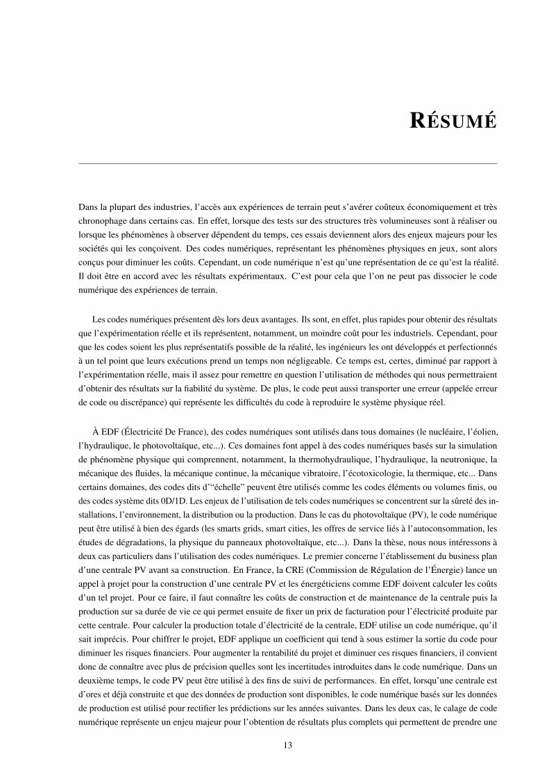
Dans la plupart des industries, l’accès aux expériences de terrain peut s’avérer coûteux économiquement et trèschronophage dans certains cas. En effet, lorsque des tests sur des structures très volumineuses sont à réaliser oulorsque les phénomènes à observer dépendent du temps, ces essais deviennent alors des enjeux majeurs pour lessociétés qui les conçoivent. Des codes numériques, représentant les phénomènes physiques en jeux, sont alorsconçus pour diminuer les coûts. Cependant, un code numérique n’est qu’une représentation de ce qu’est la réalité.Il doit être en accord avec les résultats expérimentaux. C’est pour cela que l’on ne peut pas dissocier le codenumérique des expériences de terrain.

Les codes numériques présentent dès lors deux avantages. Ils sont, en effet, plus rapides pour obtenir des résultatsque l’expérimentation réelle et ils représentent, notamment, un moindre coût pour les industriels. Cependant, pourque les codes soient les plus représentatifs possible de la réalité, les ingénieurs les ont développés et perfectionnésà un tel point que leurs exécutions prend un temps non négligeable. Ce temps est, certes, diminué par rapport àl’expérimentation réelle, mais il assez pour remettre en question l’utilisation de méthodes qui nous permettraientd’obtenir des résultats sur la fiabilité du système. De plus, le code peut aussi transporter une erreur (appelée erreurde code ou discrépance) qui représente les difficultés du code à reproduire le système physique réel.

À EDF (Électricité De France), des codes numériques sont utilisés dans tous domaines (le nucléaire, l’éolien,l’hydraulique, le photovoltaïque, etc...). Ces domaines font appel à des codes numériques basés sur la simulationde phénomène physique qui comprennent, notamment, la thermohydraulique, l’hydraulique, la neutronique, lamécanique des fluides, la mécanique continue, la mécanique vibratoire, l’écotoxicologie, la thermique, etc... Danscertains domaines, des codes dits d’“échelle” peuvent être utilisés comme les codes éléments ou volumes finis, oudes codes système dits 0D/1D. Les enjeux de l’utilisation de tels codes numériques se concentrent sur la sûreté des in-stallations, l’environnement, la distribution ou la production. Dans le cas du photovoltaïque (PV), le code numériquepeut être utilisé à bien des égards (les smarts grids, smart cities, les offres de service liés à l’autoconsommation, lesétudes de dégradations, la physique du panneaux photovoltaïque, etc...). Dans la thèse, nous nous intéressons àdeux cas particuliers dans l’utilisation des codes numériques. Le premier concerne l’établissement du business pland’une centrale PV avant sa construction. En France, la CRE (Commission de Régulation de l’Énergie) lance unappel à projet pour la construction d’une centrale PV et les énergéticiens comme EDF doivent calculer les coûtsd’un tel projet. Pour ce faire, il faut connaître les coûts de construction et de maintenance de la centrale puis laproduction sur sa durée de vie ce qui permet ensuite de fixer un prix de facturation pour l’électricité produite parcette centrale. Pour calculer la production totale d’électricité de la centrale, EDF utilise un code numérique, qu’ilsait imprécis. Pour chiffrer le projet, EDF applique un coefficient qui tend à sous estimer la sortie du code pourdiminuer les risques financiers. Pour augmenter la rentabilité du projet et diminuer ces risques financiers, il convientdonc de connaître avec plus de précision quelles sont les incertitudes introduites dans le code numérique. Dans undeuxième temps, le code PV peut être utilisé à des fins de suivi de performances. En effet, lorsqu’une centrale estd’ores et déjà construite et que des données de production sont disponibles, le code numérique basés sur les donnéesde production est utilisé pour rectifier les prédictions sur les années suivantes. Dans les deux cas, le calage de codenumérique représente un enjeu majeur pour l’obtention de résultats plus complets qui permettent de prendre une

13

décision financière basée sur plus d’informations.

Le calage de code

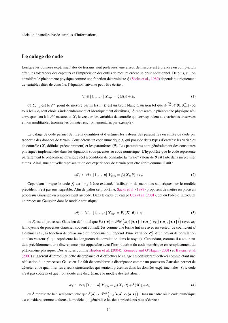
Lorsque les données expérimentales de terrains sont prélevées, une erreur de mesure est à prendre en compte. Eneffet, les tolérances des capteurs et l’imprécision des outils de mesure créent un bruit additionnel. De plus, si l’onconsidère le phénomène physique comme une fonction déterministe ξ (Sacks et al., 1989) dépendant uniquementde variables dites de contrôle, l’équation suivante peut être écrite :

∀i ∈ J1, . . . ,nK Yexpi = ξ (Xi)+ εi, (1)

où Yexpi est le ime point de mesure parmi les n, εi est un bruit blanc Gaussien tel que εiiid∼ N (0,σ2

err) (oùtous les n εi sont choisis indépendamment et identiquement distribués), ξ représente le phénomène physique réelcorrespondant à la ime mesure, etXi le vecteur des variables de contrôle qui correspondent aux variables observéeset non modifiables (comme les données environnementales par exemple).

Le calage de code permet de mieux quantifier et d’estimer les valeurs des paramètres en entrée de code parrapport à des données de terrain. Considérons un code numérique fc qui possède deux types d’entrées: les variablesde contrôle (X , définies précédemment) et les paramètres (θ). Les paramètres sont généralement des constantesphysiques implémentées dans les équations sous-jacentes au code numérique. L’hypothèse que le code représenteparfaitement le phénomène physique réel à condition de connaître la “vraie” valeur de θ est faite dans un premiertemps. Ainsi, une nouvelle représentation des expériences de terrain peut être écrite comme il suit :

M1 : ∀i ∈ J1, . . . ,nK Yexpi = fc(Xi,θ)+ εi. (2)

Cependant lorsque le code fc est long à être exécuté, l’utilisation de méthodes statistiques sur le modèleprécédent n’est pas envisageable. Afin de palier ce problème, Sacks et al. (1989) proposent de mettre en place unprocessus Gaussien en remplacement au code. Dans le cadre du calage Cox et al. (2001), ont eu l’idée d’introduireun processus Gaussien dans le modèle statistique :

M2 : ∀i ∈ J1, . . . ,nK Yexpi = Fc(Xi,θ)+ εi, (3)

où Fc est un processus Gaussien définit tel que Fc(•,•)∼PG(

mS(•,•,•,•),cS(•,•,•,•))

(avec mS

la moyenne du processus Gaussien souvent considérées comme une forme linéaire avec un vecteur de coefficient βà estimer et cS la fonction de covariance du processus qui dépend d’une variance σ2

S , d’un noyau de corrélationet d’un vecteur ψ qui représente les longueurs de corrélation dans le noyau). Cependant, comme il a été intro-duit précédemment une discrépance peut apparaître avec l’introduction du code numérique en remplacement duphénomène physique. Des articles comme Higdon et al. (2004), Kennedy and O’Hagan (2001) et Bayarri et al.(2007) suggèrent d’introduire cette discrépance et d’effectuer le calage en considérant celle-ci comme étant uneréalisation d’un processus Gaussien. Le fait de considérer la discrépance comme un processus Gaussien permet dedétecter et de quantifier les erreurs structurelles qui seraient présentes dans les données expérimentales. Si le coden’est pas coûteux et que l’on ajoute une discrépance le modèle devient alors :

M3 : ∀i ∈ J1, . . . ,nK Yexpi = fc(Xi,θ)+δ (Xi)+ εi, (4)

où δ représente la discrépance telle que δ (•)∼PG(

mδ (•,•),cδ (•,•))

. Dans un cadre où le code numériqueest considéré comme coûteux, le modèle qui généralise les deux précédents peut s’écrire :

14

M4 : ∀i ∈ J1, . . . ,nK Yexpi = Fc(Xi,θ)+δ (Xi)+ εi. (5)

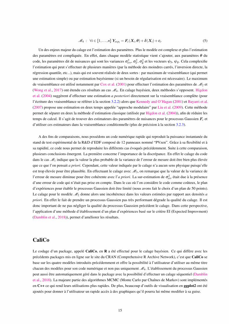
Un des enjeux majeur du calage est l’estimation des paramètres. Plus le modèle est complexe et plus l’estimationdes paramètres est compliquée. En effet, dans chaque modèle statistique vient s’ajouter, aux paramètres θ ducode, les paramètres dit de nuisances qui sont les variances σ2

err, σ2S , σ2

δet les vecteurs ψS, ψδ . Cela complexifie

l’estimation qui peut s’effectuer de plusieurs manières (par la méthode des moindres carrés, l’inversion directe, larégression quantile, etc...), mais qui est souvent réalisée de deux sortes : par maximum de vraisemblance (qui permetune estimation simple) ou par estimation bayésienne (si un besoin de régularisation est nécessaire). Le maximumde vraisemblance est utilisé notamment par Cox et al. (2001) pour effectuer l’estimation des paramètres de M2 et(Wong et al., 2017) ont étendu ces résultats au cas M4. En calage bayésien, deux méthodes s’opposent. Higdonet al. (2004) suggèrent d’effectuer une estimation a posteriori directement sur la vraisemblance complète (pourl’écriture des vraisemblance se référer à la section 3.2.2) alors que Kennedy and O’Hagan (2001) et Bayarri et al.(2007) propose une estimation en deux temps appelée “approche modulaire” par Liu et al. (2009). Cette méthodepermet de séparer en deux la méthode d’estimation classique (utilisée par Higdon et al. (2004)), afin de réduire lestemps de calcul. Il s’agit de trouver des estimateurs des paramètres de nuisances pour le processus Gaussien Fc etd’utiliser ces estimateurs dans la vraisemblance conditionnelle (plus de précision à la section 3.2.3).

A des fins de comparaisons, nous possédons un code numérique rapide qui reproduit la puissance instantanée dustand de test expérimental de la R&D d’EDF composé de 12 panneaux nommé “PVzen”. Grâce à sa flexibilité et àsa rapidité, ce code nous permet de reproduire les différents cas évoqués précédemment. Suite à cette comparaison,plusieurs conclusions émergent. La première concerne l’importance de la discrépance. En effet le calage du codedans le cas M1 indique que la valeur la plus probable de la variance de l’erreur de mesure doit être bien plus élevéeque ce que l’on pensait a priori. Cependant, cette valeur indiquée par le calage n’a aucun sens physique puisqu’elleest trop élevée pour être plausible. En effectuant le calage avec M3, on remarque que la valeur de la variance del’erreur de mesure diminue pour être cohérente avec l’a priori. La sur-estimation de σ2

err était due à la présenced’une erreur de code qui n’était pas prise en compte. Dans le cas où l’on considère le code comme coûteux, le pland’expériences pour établir le processus Gaussien doit être limité (nous avons fait le choix d’un plan de 50 points).Le calage pour le modèle M2 donne alors une incohérence dans les valeurs estimées par rapport aux densités a

priori. En effet le fait de prendre un processus Gaussien pas très performant dégrade la qualité du calage. Il estdonc important de ne pas négliger la qualité du processus Gaussien précédent le calage. Dans cette perspective,l’application d’une méthode d’établissement d’un plan d’expériences basé sur le critère EI (Expected Improvment)(Damblin et al., 2018)), permet d’améliorer les résultats.

CaliCo

Le codage d’un package, appelé CaliCo, en R a été effectué pour le calage bayésien. Ce qui diffère avec lesprécédents packages mis en ligne sur le site du CRAN (Comprehensive R Archive Network), c’est que CaliCo sebase sur les quatre modèles introduits précédemment et offre la possibilité à l’utilisateur d’utiliser au même titrechacun des modèles pour son code numérique et non pas uniquement M4. L’établissement du processus Gaussienpeut aussi être automatiquement géré dans le package avec la possibilité d’effectuer un calage séquentiel (Damblinet al., 2018). La majeure partie des algorithmes MCMC (Monte Carlo par Chaînes de Markov) sont implémentésen C++ ce qui rend leurs utilisations plus rapides. De plus, beaucoup d’outils de visualisation en ggplot2 ont étéajoutés pour donner à l’utilisateur un rapide accès à des graphiques qu’il pourra lui même modifier à sa guise.

15

Suivi de performances

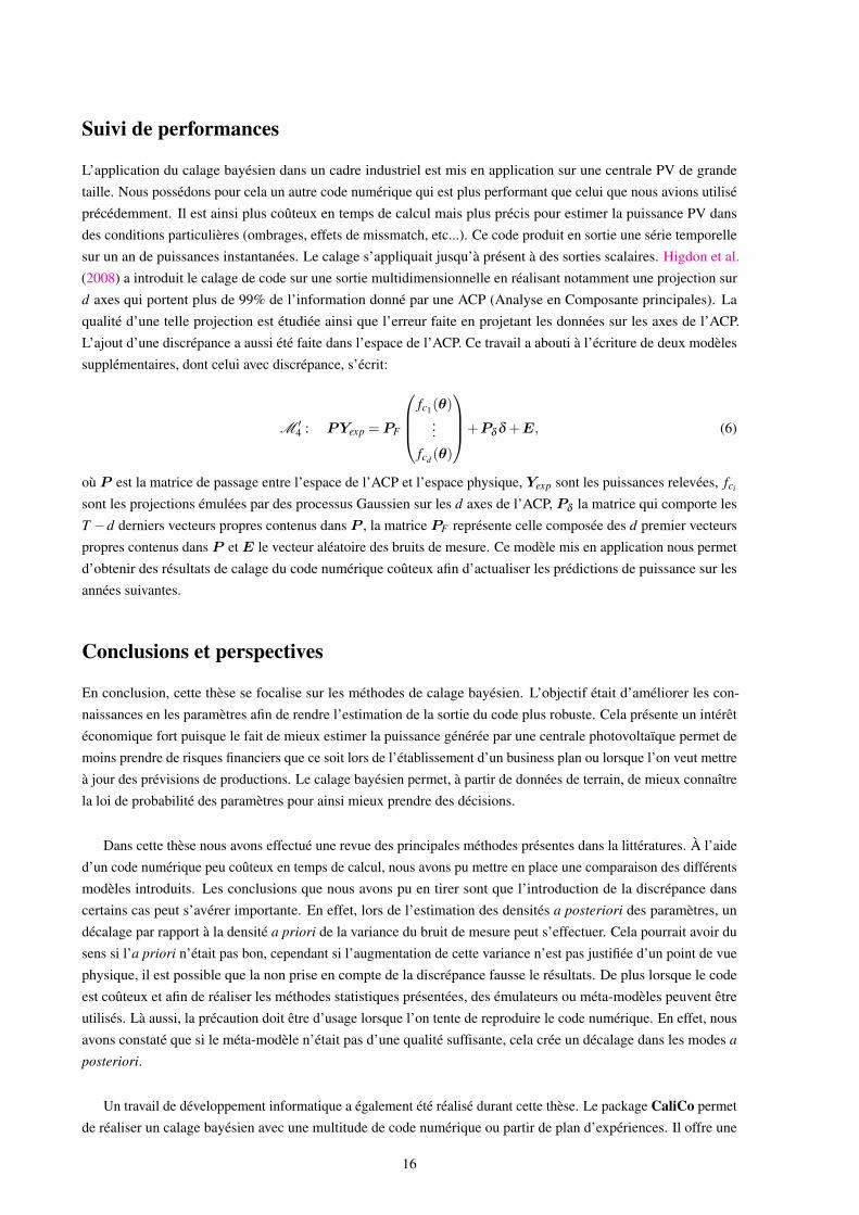
L’application du calage bayésien dans un cadre industriel est mis en application sur une centrale PV de grandetaille. Nous possédons pour cela un autre code numérique qui est plus performant que celui que nous avions utiliséprécédemment. Il est ainsi plus coûteux en temps de calcul mais plus précis pour estimer la puissance PV dansdes conditions particulières (ombrages, effets de missmatch, etc...). Ce code produit en sortie une série temporellesur un an de puissances instantanées. Le calage s’appliquait jusqu’à présent à des sorties scalaires. Higdon et al.(2008) a introduit le calage de code sur une sortie multidimensionnelle en réalisant notamment une projection surd axes qui portent plus de 99% de l’information donné par une ACP (Analyse en Composante principales). Laqualité d’une telle projection est étudiée ainsi que l’erreur faite en projetant les données sur les axes de l’ACP.L’ajout d’une discrépance a aussi été faite dans l’espace de l’ACP. Ce travail a abouti à l’écriture de deux modèlessupplémentaires, dont celui avec discrépance, s’écrit:

M ′4 : PYexp = PF

fc1(θ)

...fcd (θ)

+Pδ δ +E, (6)

où P est la matrice de passage entre l’espace de l’ACP et l’espace physique, Yexp sont les puissances relevées, fci

sont les projections émulées par des processus Gaussien sur les d axes de l’ACP, Pδ la matrice qui comporte lesT −d derniers vecteurs propres contenus dans P , la matrice PF représente celle composée des d premier vecteurspropres contenus dans P et E le vecteur aléatoire des bruits de mesure. Ce modèle mis en application nous permetd’obtenir des résultats de calage du code numérique coûteux afin d’actualiser les prédictions de puissance sur lesannées suivantes.

Conclusions et perspectives

En conclusion, cette thèse se focalise sur les méthodes de calage bayésien. L’objectif était d’améliorer les con-naissances en les paramètres afin de rendre l’estimation de la sortie du code plus robuste. Cela présente un intérêtéconomique fort puisque le fait de mieux estimer la puissance générée par une centrale photovoltaïque permet demoins prendre de risques financiers que ce soit lors de l’établissement d’un business plan ou lorsque l’on veut mettreà jour des prévisions de productions. Le calage bayésien permet, à partir de données de terrain, de mieux connaîtrela loi de probabilité des paramètres pour ainsi mieux prendre des décisions.

Dans cette thèse nous avons effectué une revue des principales méthodes présentes dans la littératures. À l’aided’un code numérique peu coûteux en temps de calcul, nous avons pu mettre en place une comparaison des différentsmodèles introduits. Les conclusions que nous avons pu en tirer sont que l’introduction de la discrépance danscertains cas peut s’avérer importante. En effet, lors de l’estimation des densités a posteriori des paramètres, undécalage par rapport à la densité a priori de la variance du bruit de mesure peut s’effectuer. Cela pourrait avoir dusens si l’a priori n’était pas bon, cependant si l’augmentation de cette variance n’est pas justifiée d’un point de vuephysique, il est possible que la non prise en compte de la discrépance fausse le résultats. De plus lorsque le codeest coûteux et afin de réaliser les méthodes statistiques présentées, des émulateurs ou méta-modèles peuvent êtreutilisés. Là aussi, la précaution doit être d’usage lorsque l’on tente de reproduire le code numérique. En effet, nousavons constaté que si le méta-modèle n’était pas d’une qualité suffisante, cela crée un décalage dans les modes a

posteriori.

Un travail de développement informatique a également été réalisé durant cette thèse. Le package CaliCo permetde réaliser un calage bayésien avec une multitude de code numérique ou partir de plan d’expériences. Il offre une

16

flexibilité du choix du modèle pour l’utilisateur. De plus, un codage des MCMC en C++ permet d’accélérer lesparties d’estimation qui sont chronophages. Des outils de visualisation basés sur ggplot2 permettent aussi de tirerprofit des réalisations du package sans difficultés.

Un dernier cas d’étude, basé sur des données de centrale photovoltaïque de grande capacité de production,a enfin été partiellement traité. Le code numérique utilisé dans ce cas est chronophage car il est basé sur desoptimisations informatiques qui alourdissent le temps de calcul mais qui améliorent ses performances. La sortie dece code est une série temporelle ce qui ne permet pas d’appliquer les différents modèles introduits précédemment.Ce problème a abouti à la formalisation de deux nouveaux modèles qui permettent, à partir d’une ACP, de trouverune sous espace vectoriel orthonormé dans lequel le calage peut être effectué. Cette formalisation a été appliquée aucas d’étude et nous a permis d’estimer les densités a posteriori des paramètres du code mais aussi de la variance deserreurs de mesures ainsi que la variance de la discrépance. La valeur de la variance de l’erreur de mesure se retrouveplus élevée que ce que l’on attendait a piori lorsque l’on utilise le modèle sans discrépance. Ce décalage est rattrapépar l’ajout de la discrépance et nous permet de conclure que l’apport de la discrépance a permis d’expliquer uneerreur qui s’était retrouvée dans la variance de l’erreur de mesure et qui représentait une erreur de code.

Cependant, les aspects prédictifs du modèle utilisant l’ACP reste à être démontré. Une validation croisée auraitpu être effectué sur un mois de données. La nécessité d’ajouter une discrépance est très discutée dans beaucoup depapiers (Kennedy and O’Hagan, 2001; Bayarri et al., 2007; Higdon et al., 2004) et fait l’objet de la validation demodèle statistique basée sur le facteur de Bayes dans Damblin et al. (2016). Une validation statistique à l’aide d’unmodèle de mélange peut aussi être envisagé comme le propose Kamary (2016). La remise en question sur la qualitédu processus Gaussien en tant qu’émulateur de code interroge sur la nécessité de prendre un plan d’expériencesbien fourni. Des travaux comme Damblin et al. (2018) permettent dans ce cas d’améliorer le plan d’expériences envue du calage bayésien. Les méthodes permettant d’utiliser des codes à sorties multidimensionnelles dans le cadredu calage découle d’un article fondateur (Higdon et al., 2008) mais ne restent pas très développés en pratique. Unprocessus Gaussien multi-fidélité pourrait aussi être envisagé en remplacement du code à sortie multidimensionnelleet ainsi être intégré dans le calage de code.

17

Intr

oduc

tion

INTRODUCTION

1.1 Economic issue . . . . . . . . . . . . . . . . . . . . . . . . . . . . . . . . . . . . . . . . . . . . 19

1.2 Physical phenomenon . . . . . . . . . . . . . . . . . . . . . . . . . . . . . . . . . . . . . . . . . 21

1.3 Several modeling approaches . . . . . . . . . . . . . . . . . . . . . . . . . . . . . . . . . . . . 22

1.3.1 A first simple model . . . . . . . . . . . . . . . . . . . . . . . . . . . . . . . . . . . . . 22

1.3.2 Advanced electrical models . . . . . . . . . . . . . . . . . . . . . . . . . . . . . . . . . 23

1.4 Numerical codes . . . . . . . . . . . . . . . . . . . . . . . . . . . . . . . . . . . . . . . . . . . 25

1.4.1 General framework . . . . . . . . . . . . . . . . . . . . . . . . . . . . . . . . . . . . . . 25

1.4.2 Sources of uncertainties . . . . . . . . . . . . . . . . . . . . . . . . . . . . . . . . . . . 25

1.4.3 Python code . . . . . . . . . . . . . . . . . . . . . . . . . . . . . . . . . . . . . . . . . . 26

1.4.4 Dymola code . . . . . . . . . . . . . . . . . . . . . . . . . . . . . . . . . . . . . . . . . 27

1.5 Thesis organization . . . . . . . . . . . . . . . . . . . . . . . . . . . . . . . . . . . . . . . . . . 30

In many industrial fields, numerical experiments have become more and more popular over the last few years.Field experiments are often really expensive and getting results from the real phenomenon is quite long. To limitthis investment, numerical simulations are run as a substitute for field experiments (Santner et al., 2013; Fanget al., 2005). As numerical simulations intend to be as close as possible to the physical system, they have beencontinuously improved. However, the development of computer processors did not catch up with this evolutionand some numerical simulations are still greedy in computational time (Sacks et al., 1989). Moreover, a differencebetween the numerical code and experiments is often observed. If there exists a bias between the code and thereality, what is the uncertainty in using it as a proxy of the physical system? Bayarri et al. (2007) introduce thenotion of validation which consists in comparing the code outputs to the field experiments. Such a task can bedifficult to achieve since it needs expensive field experiments and outputs from a code, often long to run. All alongthis thesis, we will use the word “code” as a proxy for numerical code, sometimes also called numerical model,simulator or computational code and field experiment for real world experiment.

In that respect, EDF (Électricité De France) uses numerical simulations in many fields, in particular to estimatethe power produced by a photovoltaic (PV) plant. This thesis is motivated by the uncertainty quantification andcalibration of a numerical code that intends to estimate the power produced by a PV plant. In this introduction, wewill present the economic context that explains the needs of EDF for such a study. Then, a brief explanation of howa PV panel works is given that is followed by details on the different physical models developed by EDF. Finally,the numerical codes, used as application cases in this thesis, are detailed and presented in the last section.

1.1 Economic issue

Due to global warming, new “fuel-free” technologies are increasingly being developed. EDF focuses its research onsome of them which are, without being exhaustive, the photovolatic, wind turbines or concentrated solar power(CSP). In each field the same economic problems appear especially in the photovoltaic (PV) where more andmore PV plants are built in France and all around the would. The goal for energy suppliers such as EDF is to becompetitive in this new market. In France, the apparition of new plants is regulated by an entity called CRE (EnergyRegulation Commission). The right to build and manage a new plant usually comes by winning a bidding call for

19

Intr

oduc

tion

Chapter 1 – Introduction

project. The business model of such a project is particularly based on a factor called the levelized cost of energyalso named LCOE.

The average minimum cost at which electricity must be sold in order to break-evenover the lifetime of the project.

LCOE

It can be written as:

LCOE =sum o f actualized costs over the li f etime

sum o f electrical energy produced over li f etime=

∑nt=1

It+Mt(1+r)t

∑nt=1

Et(1+r)t

, (1.1)

where It stands for the investment expenditures in the year t, Mt for the operations and maintenance expenditures inthe year t, Et for the electrical energy generated in the year t, r for the discount rate and n for the expected lifetimeof the system or power station.

The costs are relatively well estimated. Based on previous experience, the operational expenditures (also namedOPEX, which encompass the operations and maintenance expenditures) and the capital expenditures (also calledCAPEX, which cover investment expenditures It ) are approximated with a narrow credibility interval. The CAPEXrepresents the invested money for building a photovoltaic plant and are fixed costs, when the OPEX is the moneyspent to build and maintain the photovolatic plant and stands for the variable costs. However, to predict the totalpower generated over the lifetime of the plant, energy suppliers use a homemade or commercial numerical code.For the uncertainty quantification of the code, the actual methodologies used give credibility intervals around ±8%of the output of the code. A compromise is found between the risk and the price based on the estimated uncertainty.This compromise tends to have a LCOE secure for investors but it increases the price of the project. Other energysupplier companies, which could have more accurately predicted the power or have a more aggressive policy on theestablishment of business plans, could win the project. The main stake is to better assess the credibility interval onthe power produced so that even the estimation of the less power produced is better than the final power estimationof the competition.

Once EDF has won the call for project, the PV plant is built in the specific location. When its activationis effective, data of power production are recorded. After some time, EDF engineers can compare the estima-tion made in the business plan to the real power produced. If, as expected, the prediction is lower than realpower gathered on the field, the electricity price based on the business plan is no longer adequate. A new sim-ulation can be run, based on these new data, which better estimates the power produced for the next few years.The business plan can then be updated based on the new estimation. This operation is called performance monitoring.

In France the economical stakes are important because it is the fifth photovoltaic field in Europe. The estimationof the total production capacity is more than 400 GWp. Wp stands for Watt peak which represents the powerdelivered by a photovolatic panel or plant under nominal conditions (1000 W/m2 of enlightening and a temperatureof 25°C). The development deadlines are also shorter in photovolatic (3-4 years) than onshore wind turbine (7-9years). The costs of the electricity produced by the photovoltaic is decreasing (it was more than 200 e/MWh in2012 and it was equal to 55 e/MWh in 2018 for large scaled PV plants). So far, in France only 8,159 MW ofPV capacity is installed. In 2018 EDF has announced a Solar Plan which aims to install 30 GW of photovoltaicpower between 2020 and 2035. A major part of this 30 GW will be constituted of by large PV plants. The resourcesmobilized by the EDF Group are the identification of the land to be mobilized, the mobilization of the subcontractingchain and EDF’s partners, the development of self-consumption offers, the cooperation with public authorities to

20

Intr

oduc

tion

1.2. Physical phenomenon

make large areas available, the development of an industrial model adapted to the challenge, etc... In that contextEDF is looking to better control the uncertainties made by the production estimations to limit financial risks whenestablishing the project.

The aim of this thesis is to quantify the uncertainty of the numerical codes used by EDF. Based on Bayesiancalibration, the main framework will be the performance monitoring, where recorded power data are available. Then,the new predicted power can then be compared to the estimated one in the business plan and quantify plausibleearnings.

1.2 Physical phenomenon

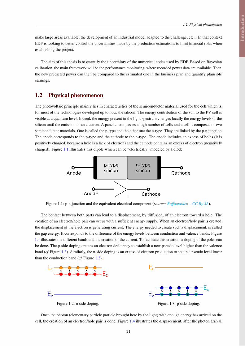
The photovoltaic principle mainly lies in characteristics of the semiconductor material used for the cell which is,for most of the technologies developed up to now, the silicon. The energy contribution of the sun to the PV cell isvisible at a quantum level. Indeed, the energy present in the light spectrum changes locally the energy levels of thesilicon until the emission of an electron. A panel encompasses a high number of cells and a cell is composed of twosemiconductor materials. One is called the p-type and the other one the n-type. They are linked by the p-n junction.The anode corresponds to the p-type and the cathode to the n-type. The anode includes an excess of holes (it ispositively charged, because a hole is a lack of electron) and the cathode contains an excess of electron (negativelycharged). Figure 1.1 illustrates this dipole which can be “electrically” modeled by a diode.

Figure 1.1: p-n junction and the equivalent electrical component (source: Raffamaiden – CC By SA).

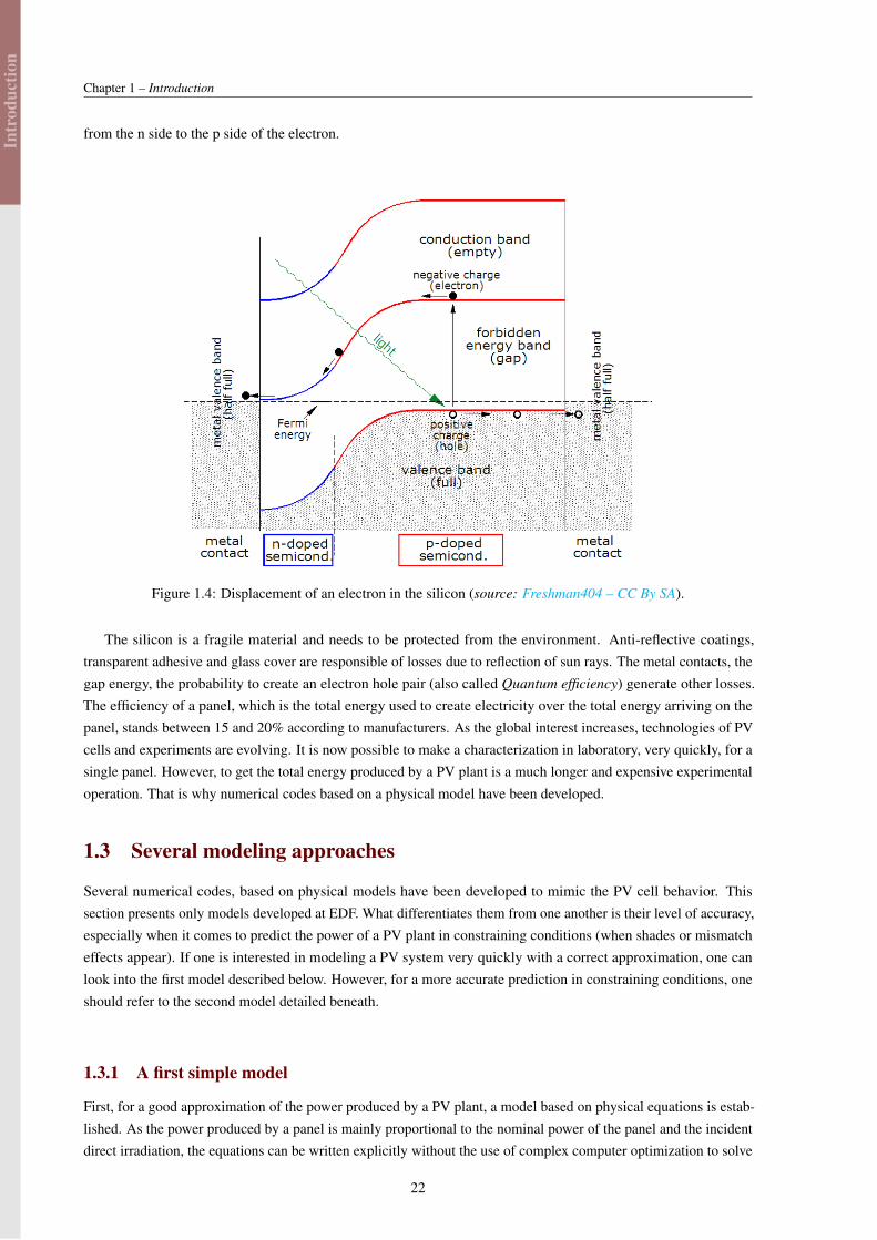
The contact between both parts can lead to a displacement, by diffusion, of an electron toward a hole. Thecreation of an electron/hole pair can occur with a sufficient energy supply. When an electron/hole pair is created,the displacement of the electron is generating current. The energy needed to create such a displacement, is calledthe gap energy. It corresponds to the difference of the energy levels between conduction and valence bands. Figure1.4 illustrates the different bands and the creation of the current. To facilitate this creation, a doping of the poles canbe done. The p-side doping creates an electron deficiency to establish a new pseudo level higher than the valenceband (cf Figure 1.3). Similarly, the n-side doping is an excess of electron production to set up a pseudo level lowerthan the conduction band (cf Figure 1.2).

Figure 1.2: n side doping. Figure 1.3: p side doping.

Once the photon (elementary particle particle brought here by the light) with enough energy has arrived on thecell, the creation of an electron/hole pair is done. Figure 1.4 illustrates the displacement, after the photon arrival,

21

Intr

oduc

tion

Chapter 1 – Introduction

from the n side to the p side of the electron.

Figure 1.4: Displacement of an electron in the silicon (source: Freshman404 – CC By SA).

The silicon is a fragile material and needs to be protected from the environment. Anti-reflective coatings,transparent adhesive and glass cover are responsible of losses due to reflection of sun rays. The metal contacts, thegap energy, the probability to create an electron hole pair (also called Quantum efficiency) generate other losses.The efficiency of a panel, which is the total energy used to create electricity over the total energy arriving on thepanel, stands between 15 and 20% according to manufacturers. As the global interest increases, technologies of PVcells and experiments are evolving. It is now possible to make a characterization in laboratory, very quickly, for asingle panel. However, to get the total energy produced by a PV plant is a much longer and expensive experimentaloperation. That is why numerical codes based on a physical model have been developed.

1.3 Several modeling approaches

Several numerical codes, based on physical models have been developed to mimic the PV cell behavior. Thissection presents only models developed at EDF. What differentiates them from one another is their level of accuracy,especially when it comes to predict the power of a PV plant in constraining conditions (when shades or mismatcheffects appear). If one is interested in modeling a PV system very quickly with a correct approximation, one canlook into the first model described below. However, for a more accurate prediction in constraining conditions, oneshould refer to the second model detailed beneath.

1.3.1 A first simple model

First, for a good approximation of the power produced by a PV plant, a model based on physical equations is estab-lished. As the power produced by a panel is mainly proportional to the nominal power of the panel and the incidentdirect irradiation, the equations can be written explicitly without the use of complex computer optimization to solve

22

Intr

oduc

tion

1.3. Several modeling approaches

eventually challenging equations. To consider the losses described in Section 1.2, parameters are implemented inthe model and can encompass the module photo-conversion efficiency or the module temperature coefficient forexample (more details are given in Section 1.4.3). This model, that does not require any optimization to get theresolution of eventual differential equations, is quick to implement but presents some limitations.

1.3.2 Advanced electrical models

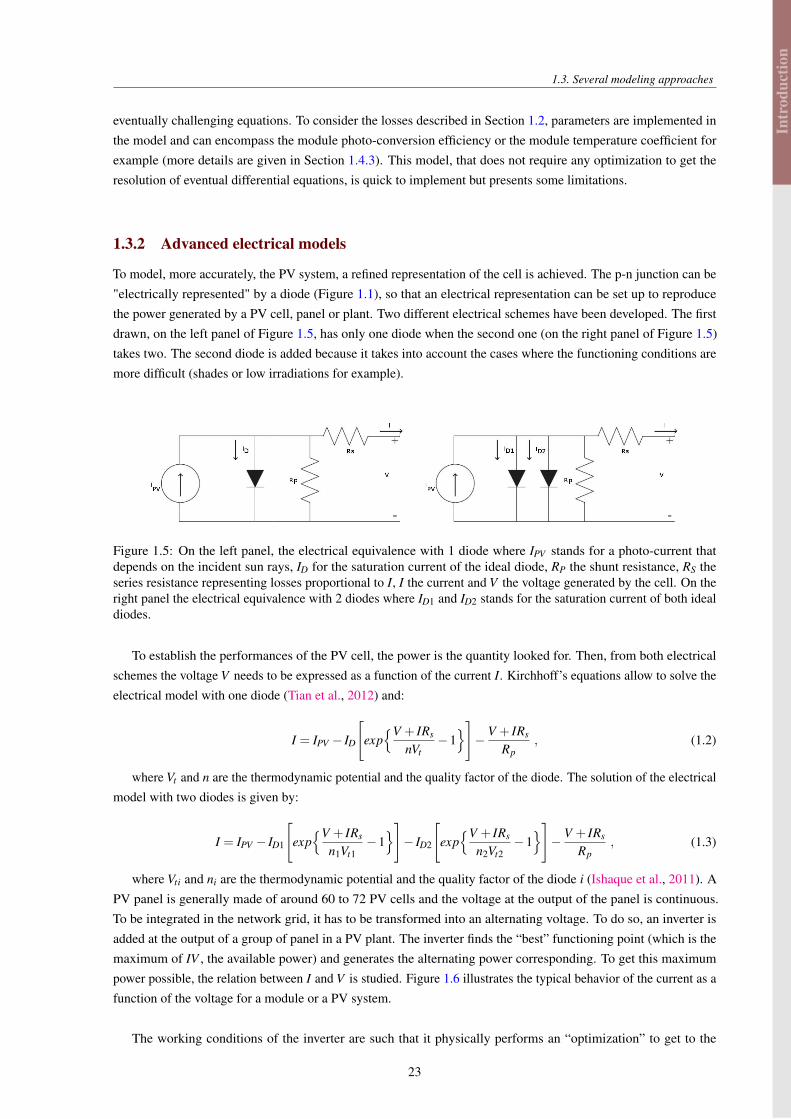
To model, more accurately, the PV system, a refined representation of the cell is achieved. The p-n junction can be"electrically represented" by a diode (Figure 1.1), so that an electrical representation can be set up to reproducethe power generated by a PV cell, panel or plant. Two different electrical schemes have been developed. The firstdrawn, on the left panel of Figure 1.5, has only one diode when the second one (on the right panel of Figure 1.5)takes two. The second diode is added because it takes into account the cases where the functioning conditions aremore difficult (shades or low irradiations for example).

Figure 1.5: On the left panel, the electrical equivalence with 1 diode where IPV stands for a photo-current thatdepends on the incident sun rays, ID for the saturation current of the ideal diode, RP the shunt resistance, RS theseries resistance representing losses proportional to I, I the current and V the voltage generated by the cell. On theright panel the electrical equivalence with 2 diodes where ID1 and ID2 stands for the saturation current of both idealdiodes.

To establish the performances of the PV cell, the power is the quantity looked for. Then, from both electricalschemes the voltage V needs to be expressed as a function of the current I. Kirchhoff’s equations allow to solve theelectrical model with one diode (Tian et al., 2012) and:

I = IPV − ID

[expV + IRs

nVt−1]− V + IRs

Rp, (1.2)

where Vt and n are the thermodynamic potential and the quality factor of the diode. The solution of the electricalmodel with two diodes is given by:

I = IPV − ID1

[expV + IRs

n1Vt1−1]− ID2

[expV + IRs

n2Vt2−1]− V + IRs

Rp, (1.3)

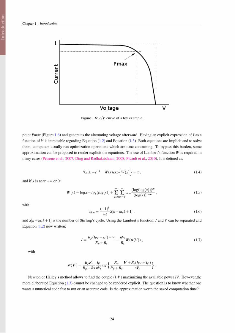
where Vti and ni are the thermodynamic potential and the quality factor of the diode i (Ishaque et al., 2011). APV panel is generally made of around 60 to 72 PV cells and the voltage at the output of the panel is continuous.To be integrated in the network grid, it has to be transformed into an alternating voltage. To do so, an inverter isadded at the output of a group of panel in a PV plant. The inverter finds the “best” functioning point (which is themaximum of IV , the available power) and generates the alternating power corresponding. To get this maximumpower possible, the relation between I and V is studied. Figure 1.6 illustrates the typical behavior of the current as afunction of the voltage for a module or a PV system.

The working conditions of the inverter are such that it physically performs an “optimization” to get to the

23

Intr

oduc

tion

Chapter 1 – Introduction

Figure 1.6: I/V curve of a toy example.

point Pmax (Figure 1.6) and generates the alternating voltage afterward. Having an explicit expression of I as afunction of V is intractable regarding Equation (1.2) and Equation (1.3). Both equations are implicit and to solvethem, computers usually run optimization operations which are time consuming. To bypass this burden, someapproximation can be proposed to render explicit the equations. The use of Lambert’s function W is required inmany cases (Petrone et al., 2007; Ding and Radhakrishnan, 2008; Picault et al., 2010). It is defined as:

∀x≥−e−1 W (x)exp

W (x)= x , (1.4)

and if x is near +∞ or 0:

W (x) = logx− log(log(x))+∞

∑k=0

∞

∑m=1

ckm(log(log(x)))m

(log(x))k+m , (1.5)

with

ckm =(−1)k

m!S[k+m,k+1] , (1.6)

and S[k+m,k+1] is the number of Stirling’s cycle. Using the Lambert’s function, I and V can be separated andEquation (1.2) now written:

I =Rp(IPV + ID)−V

Rp +Rs− nVt

RsW (α(V )) , (1.7)

with

α(V ) =RpRs

Rp +RsID

nVtexp Rp

Rp +Rs

V +Rs(IPV + ID)

nVt

.

Newton or Halley’s method allows to find the couple (I,V ) maximizing the available power IV . However,themore elaborated Equation (1.3) cannot be changed to be rendered explicit. The question is to know whether onewants a numerical code fast to run or an accurate code. Is the approximation worth the saved computation time?

24

Intr

oduc

tion

1.4. Numerical codes

1.4 Numerical codes

In this section, we detail the general framework and notations of the numerical codes used in this thesis and weintroduce the main sources of uncertainties that can be found in this context. Then we present, in details, the twonumerical codes further used in this work.

1.4.1 General framework

A computer code generally depends on two kinds of inputs: variables and parameters. The variables representthe input variables (also called controllable variables in Higdon et al. (2008) or general inputs in Plumlee (2017))which are set during a field experiment and can encompass environmental variables which can be measured in fieldexperiments. In contrast, the parameters are generally interpreted as physical constants defining the mathematicalmodel of the system of interest, but can also contain the so-called tuning parameters, which have no physicalinterpretation. They have to be set by the user to run the code and chosen carefully to make the code mimic the realphysical phenomenon. The code can be mathematically represented by a function fc. Let us note in what followsthat, θ ∈Q ⊂ Rp to represent the parameter vector and x ∈H ⊂ Rd which is the variable vector. The space Q iscalled the input parameter space and H the input variable space. The physical quantity of interest (QOI) is denotedby ζ and only depends on variables in vector x ∈H because the parameter vector θ has no counterpart in fieldexperiments.

A code output is then written as fc(x,θ) (considered as a deterministic code all along the thesis) whereas ζ (x)

denotes the physical phenomenon for the same variable x. This is of course an idealized formalization, in whichwe assume that the code variables x are exhaustive to describe the phenomenon of interest, in the sense that thequantity to be predicted can take a single deterministic value ζ (x) for a given x.

1.4.2 Sources of uncertainties

In general, there are two main kinds of uncertainties considered: the epistemic and the statistical. The statisticaluncertainty represents the random fluctuations of the input variables, and the associated measurement errors andthe epistemic uncertainty comes from the uncertainty on parameters, that one could in principle know but doesnot in practice. The latter can be estimated but can also be reduced as the number of experiments increases. Theuncertainties relative to the numerical code are then epistemic. The code is deterministic so no variability is visiblebetween two launches. In this thesis, we focus only on the epistemic uncertainties that are detailed below.

The numerical code takes two inputs that are uncertain: θ and X . In the calibration framework, only theuncertainty on θ is considered because we do not know the true value of θ and we need to adjust it.

In the PV plant context, θ represents physical constants or manufacturer values that are carrying uncertainty.Indeed, the building process of a PV panel encompasses tolerances at each step of the fabrication. At the end of thechain, the parameter, that characterizes the nominal power of the panel for example, might be altered. The inputvariablesX represent mainly meteorological data. These are also carrying uncertainty because in both, predictionor performance monitoring, contexts, X is averaged from previous data where modification due to global warmingis added.

This thesis focuses only on parametric uncertainties, because the main aim is to calibrate the parameter vector θgiven a data set, the uncertainty of the input variable being out of the scope of this study. EDF experts judge that

25

Intr

oduc

tion

Chapter 1 – Introduction

parameter uncertainty and input variable uncertainty are each responsible for about 4% of the output variability.

1.4.3 Python code

Code

The Python code has been developed based on the first physical model described in Section 1.3.1. It implements thephysical equations that encompass production approximation estimation but also the losses relative to the panel. Asno optimization are needed in this code, it runs very fast (about 36µs each run). The code, that does not take intoaccount the inverter, produces an estimation of the instantaneous power. That means:

fc : H ×Q→ R

(x,θ) 7→ y .(1.8)

The code depends on some parameter vector θ and input variables x detailed as follows: θ =

η

µt

nt

al

ar

ninc

and

x=

t

L

l

Ig

Id

Te

.

The physical meaning of the parameters θ is explained below (Duffie and Beckman, 2013):

• η : module photo-conversion efficiency in nominal test conditions (1000W/m2, 25°C),

• µt : module temperature coefficient (the efficiency decreases when the temperature rises) in %/°C,

• nt : reference temperature for the normal operating conditions of the module in °C,

• al : reflection power of the ground (albedo),

• ar: describes the transmission of the radiation as a function of the incidence angle of solar rays, whichdepends on optical properties and the cleanliness,

• ninc: transmission factor for normal incidence.

The input variables x contain all measurable data:

• t: the UTC time since the beginning of the year in s,

• L: the latitude in °,

• l: the longitude in °,

• Ig: global irradiation (normal incidence of the sun rays to the panel) in W/m2,

• Id : diffuse irradiation (horizontal incidence of the sun rays to the panel) in W/m2,

26

Intr

oduc

tion

1.4. Numerical codes

• Te: ambient temperature in °C.

Note that temporal aspects are taken into account through the input variables. We do not consider any delay inthe PV reaction to the forcing conditions. Time t indicates here a snap shot corresponding to the instant when thepower has to be computed. This code only focuses on a specific time and if the evolution of the power over a day iswhat we look for, a repetition over the specific durations has to be made. This operation has to consider the numberof time steps available. For example, if 300 configurations of x are accessible for one day, the code will have to beexecuted 300 times to have the power evolution over a day. For the rest of this thesis, we will denote the code outputreferring to the ith time step by fc(xi,θ) and by fc(X,θ) the code outputs corresponding to the whole time framecontained in matrix X.

Experimental data

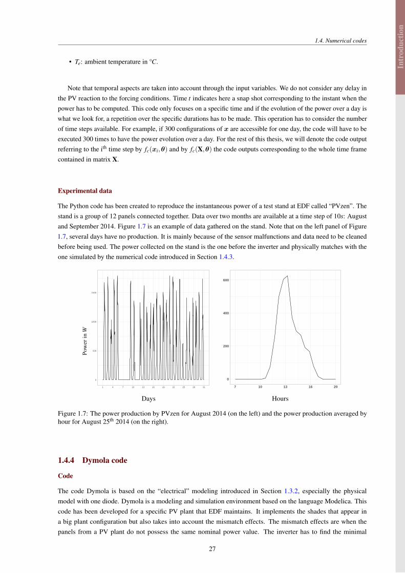
The Python code has been created to reproduce the instantaneous power of a test stand at EDF called “PVzen”. Thestand is a group of 12 panels connected together. Data over two months are available at a time step of 10s: Augustand September 2014. Figure 1.7 is an example of data gathered on the stand. Note that on the left panel of Figure1.7, several days have no production. It is mainly because of the sensor malfunctions and data need to be cleanedbefore being used. The power collected on the stand is the one before the inverter and physically matches with theone simulated by the numerical code introduced in Section 1.4.3.

Pow

erin

W

0

500

1000

1500

1 4 7 10 13 16 19 22 25 28 31

0

200

400

600

7 10 13 16 20

Days Hours

Figure 1.7: The power production by PVzen for August 2014 (on the left) and the power production averaged byhour for August 25th 2014 (on the right).

1.4.4 Dymola code

Code

The code Dymola is based on the “electrical” modeling introduced in Section 1.3.2, especially the physicalmodel with one diode. Dymola is a modeling and simulation environment based on the language Modelica. Thiscode has been developed for a specific PV plant that EDF maintains. It implements the shades that appear ina big plant configuration but also takes into account the mismatch effects. The mismatch effects are when thepanels from a PV plant do not possess the same nominal power value. The inverter has to find the minimal

27

Intr

oduc

tion

Chapter 1 – Introduction

one and not the averaged. Mismatch effects is also a concern when one or several cells are shaded but not thewhole panel. Shunt resistances are then activated so this part of the panel does not affect the panel overall production.

This code is then much longer to run than the previous one (about 20s for each call) but the output is a temporaltrajectory over one year of the instantaneous power with the time step of 900s. This means that, for n points in thetrajectory:

fc : Q→ Rn

θ 7→ y .(1.9)

This numerical code does not take X as input variables because they are implicitly implemented in Dymola.As a matter of fact, X represent the meteorological, the mismatch data and the projected rays files for one yearcorresponding to the n points produced by fc. The mismatch and the projected rays files are input data that give theinformation of the mismatch effects and the shades on the PV plant panels we are focusing on. In these conditions,the output power is more complex to determine. The parameter vector θ takes 26 components that we will not detailhere. The parameter vector encompasses those which have an electrical meaning such as Ipv, Rp or Rs of Figure 1.5(on the left panel) but also those which characterize the inverter. That means the output given by the Dymola codecorresponds to the power after the optimization performed by the inverter.

Experimental data

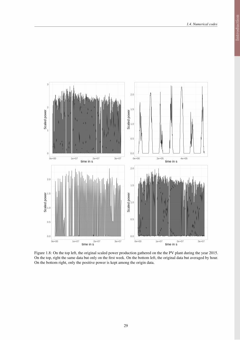
The data available for the Dymola code is the power gathered during one year 2015 (sometimes data are partiallycollected). Data are scaled in Figure (1.8) for confidentiality matters. Identically as in Figure 1.7, there is somedays where the production is null. These issues are common and also correspond to recording errors. Figure 1.8represents the temporal series given by the PV plant for the year 2015.

28

Intr

oduc

tion

1.4. Numerical codes

0

1

2

3

0e+00 1e+07 2e+07 3e+07time in s

Sca

led

pow

er

0.0

0.5

1.0

1.5

2.0

0e+00 2e+05 4e+05time in s

Sca

led

pow

er

0.0

0.5

1.0

1.5

2.0

0e+00 1e+07 2e+07 3e+07time in s

Sca

led

pow

er

0.0

0.5

1.0

1.5

2.0

0e+00 1e+07 2e+07 3e+07time in s

Sca

led

pow

er

Figure 1.8: On the top left, the original scaled power production gathered on the the PV plant during the year 2015.On the top, right the same data but only on the first week. On the bottom left, the original data but averaged by hour.On the bottom right, only the positive power is kept among the origin data.

29

Intr

oduc

tion

Chapter 1 – Introduction

1.5 Thesis organization

This thesis presents the work done on Bayesian calibration especially conditioned by the two different applicationcases detailed above. First, Chapter 2 recalls the main tools in sensitivity analysis, design of experiments, principlecomponent analysis, Monte Carlo Markov chains and Gaussian processes for a good understanding of BayesianCalibration. Chapter 3 gives a state of the art of Bayesian calibration methods. This chapter uses the applicationcase of the Python code to illustrate and compare the different statistical models that are existing. Then, Chapter 4presents a package, called CaliCo, that completes Bayesian calibration in R which has been developed in the frameof this thesis. Chapter 5 illustrates a comprehensive industrial study of calibration using the Dymola code and datafrom a real PV plant. The document then concludes with a discussion and perspectives to be explored.

30

Cha

pter

2

CHAPTER2STATISTICAL TOOLS FOR NUMERICAL

CODE CALIBRATION

2.1 Sensitivity analysis . . . . . . . . . . . . . . . . . . . . . . . . . . . . . . . . . . . . . . . . . . 33

2.1.1 Morris method . . . . . . . . . . . . . . . . . . . . . . . . . . . . . . . . . . . . . . . . 33

2.1.2 Sobol indices . . . . . . . . . . . . . . . . . . . . . . . . . . . . . . . . . . . . . . . . . 39

2.2 Kriging / Gaussian processes . . . . . . . . . . . . . . . . . . . . . . . . . . . . . . . . . . . . . 42

2.2.1 General framework . . . . . . . . . . . . . . . . . . . . . . . . . . . . . . . . . . . . . . 42

2.2.2 Parameter estimation . . . . . . . . . . . . . . . . . . . . . . . . . . . . . . . . . . . . . 45

2.2.3 Covariance functions . . . . . . . . . . . . . . . . . . . . . . . . . . . . . . . . . . . . . 47

2.2.4 Gaussian process-based optimization . . . . . . . . . . . . . . . . . . . . . . . . . . . . 48

2.3 Design of experiments . . . . . . . . . . . . . . . . . . . . . . . . . . . . . . . . . . . . . . . . 51

2.3.1 Sampling criteria . . . . . . . . . . . . . . . . . . . . . . . . . . . . . . . . . . . . . . . 51

2.3.2 Distance between the points criteria . . . . . . . . . . . . . . . . . . . . . . . . . . . . . 52

2.4 Principal component analysis (PCA) . . . . . . . . . . . . . . . . . . . . . . . . . . . . . . . . . 54

2.4.1 Distance . . . . . . . . . . . . . . . . . . . . . . . . . . . . . . . . . . . . . . . . . . . . 54

2.4.2 Moments of inertia . . . . . . . . . . . . . . . . . . . . . . . . . . . . . . . . . . . . . . 55

2.4.3 Axis of minimum inertia . . . . . . . . . . . . . . . . . . . . . . . . . . . . . . . . . . . 56

2.4.4 Contribution to the total inertia . . . . . . . . . . . . . . . . . . . . . . . . . . . . . . . . 58

2.4.5 Graphical representations . . . . . . . . . . . . . . . . . . . . . . . . . . . . . . . . . . . 58

2.5 Monte Carlo Markov Chains techniques . . . . . . . . . . . . . . . . . . . . . . . . . . . . . . . 61

2.5.1 Gibbs sampler . . . . . . . . . . . . . . . . . . . . . . . . . . . . . . . . . . . . . . . . 62

2.5.2 Metropolis Hastings . . . . . . . . . . . . . . . . . . . . . . . . . . . . . . . . . . . . . 63

2.5.3 Metropolis within Gibbs . . . . . . . . . . . . . . . . . . . . . . . . . . . . . . . . . . . 65

2.5.4 Improvements of the Metropolis Hastings . . . . . . . . . . . . . . . . . . . . . . . . . . 65

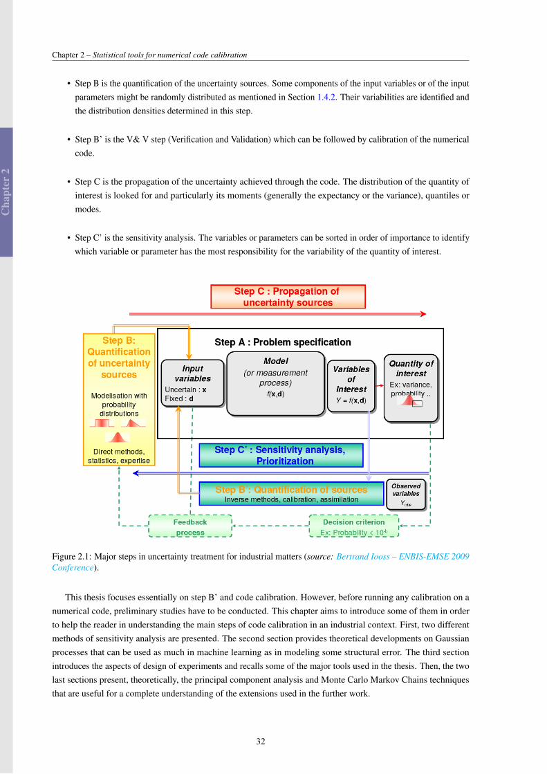
Uncertainty Quantification (UQ) in an industrial context has become important over the last few years. All alongthe process in an industrial cycle, from the research to the in-service and maintenance, UQ has an equivalent impacton business and risk reliability. However, the procedure for establishing the impact of the variability of severalquantities on the output of interest has to be performed in multiple steps. From the identification of which parameteris responsible for the most of the output variation to the propagation of uncertainty, there is several steps that aredetailed in Rocquigny (2009). Figure 2.1 is a graphical representation of the main steps in the UQ in an industrialcontext:

• Step A is the problem specification. An identification of the quantities of interest, input variables, inputparameters, and of the numerical codes have to be done.

31

Cha

pter

2

Chapter 2 – Statistical tools for numerical code calibration

• Step B is the quantification of the uncertainty sources. Some components of the input variables or of the inputparameters might be randomly distributed as mentioned in Section 1.4.2. Their variabilities are identified andthe distribution densities determined in this step.

• Step B’ is the V& V step (Verification and Validation) which can be followed by calibration of the numericalcode.

• Step C is the propagation of the uncertainty achieved through the code. The distribution of the quantity ofinterest is looked for and particularly its moments (generally the expectancy or the variance), quantiles ormodes.

• Step C’ is the sensitivity analysis. The variables or parameters can be sorted in order of importance to identifywhich variable or parameter has the most responsibility for the variability of the quantity of interest.

Figure 2.1: Major steps in uncertainty treatment for industrial matters (source: Bertrand Iooss – ENBIS-EMSE 2009Conference).

This thesis focuses essentially on step B’ and code calibration. However, before running any calibration on anumerical code, preliminary studies have to be conducted. This chapter aims to introduce some of them in orderto help the reader in understanding the main steps of code calibration in an industrial context. First, two differentmethods of sensitivity analysis are presented. The second section provides theoretical developments on Gaussianprocesses that can be used as much in machine learning as in modeling some structural error. The third sectionintroduces the aspects of design of experiments and recalls some of the major tools used in the thesis. Then, the twolast sections present, theoretically, the principal component analysis and Monte Carlo Markov Chains techniquesthat are useful for a complete understanding of the extensions used in the further work.

32

Cha

pter

2

2.1. Sensitivity analysis

2.1 Sensitivity analysis

The quantification of the influence of each input parameter on the output is the task performed by sensitivity analysis.It is interesting to access such an information because if the numerical code is time consuming, it can be helpful tofocus on a reduced number of parameters. In that sense, sensitivity analysis (SA) can be considered as a prerequisitefor model building in any setting (Saltelli et al., 2000). SA has a different meaning in different contexts. For anengineer, it could mean to move each component of the input parameter vector at the same range and comparethe impacts on the quantity of interest. For a statistician, SA is the study of the variation of the distribution of thedensity of the quantity of interest according to the change of specific parameters.

There are two major categories in SA: global and local methods. Local SA tends to quantify the impact ofa parameter around reference values. It is mainly done with partial derivatives. This kind of analysis is usefulwhen one is interested in understanding the behavior of the physical model nearby these values. However, thesemethods do not allow to study the effect of the input parameters on the output when they have an important area ofuncertainty. Contrary to local SA, global SA aims to study the variability of the quantity of interest driven by inputparameters variation on all their area of uncertainty. In this section, we present only global SA methods mainlybecause in this thesis we are interested on the overall impact of the parameters on the variability of the quantity ofinterest.

Global SA can be performed in several different ways. First, screening methods allow to explore quickly thevariability of the output, given by a numerical code, induced by a variation of the, potentially large, input parametervector. The importance criterion in such methods is the amplitude of the variations of the code output obtained fordifferent input parameter values. Screening methods can also be categorized but we only focus on Morris methodSection 2.1.1 (Morris, 1991) because it requires less assumptions about the model compared to the other screeningmethods. These methods only allow to identify the non-influent parameters. If one is interested in classifying byorder of importance the parameter influence, sensibility indices can be used. Sensibility indices are defined as ameasure of the influence of an input parameter on the variability of the output. If the chosen measure of importanceis the variance, then the indices are called Sobol indices (Sobol’, 1990) and are presented in Section 2.1.2. However,these methods require a lot of code calls and if the code is time consuming they become quickly intractable. Toestimate, with a limited computational impact, sensitivity indices, smoothing methods or surrogate of the codefunction have been developed. For example, Sudret (2008) demonstrates that Sobol indices straightforwardly arisefrom the chaos polynomial decomposition. Kriging surrogate also allows to obtain analytically the sensitivityindices formulation as it is shown in Oakley and O’Hagan (2004); Marrel et al. (2009). Da Veiga (2015) alsointroduced global SA methods which use dependence measures as the mutual information, the distance correlationor the Hilbert-Schmidt Independence Criterion (HSIC). Then, De Lozzo and Marrel (2016) have extended this workfor a screening purpose and allow to decrease the computational time burden.

2.1.1 Morris method

Morris method aims to evaluate the influence of each input parameter by considering the impact of its variation onthe output considering the other ones as constant. This way to operate consists in moving each parameter one at atime ("One At a Time" or OAT method). Then, the input parameter space is discretized on a grid.

Sampling space

Since the parameter range values are not all of the same order, the sampling design of the Morris method isstandardized over the interval [0,1]. Thus, for p parameters, the sampling plan will be contained in a hypercubeω = [0,1]p. To generate a comparable variation for each parameters, a step δ is defined. For each parameter, the

33

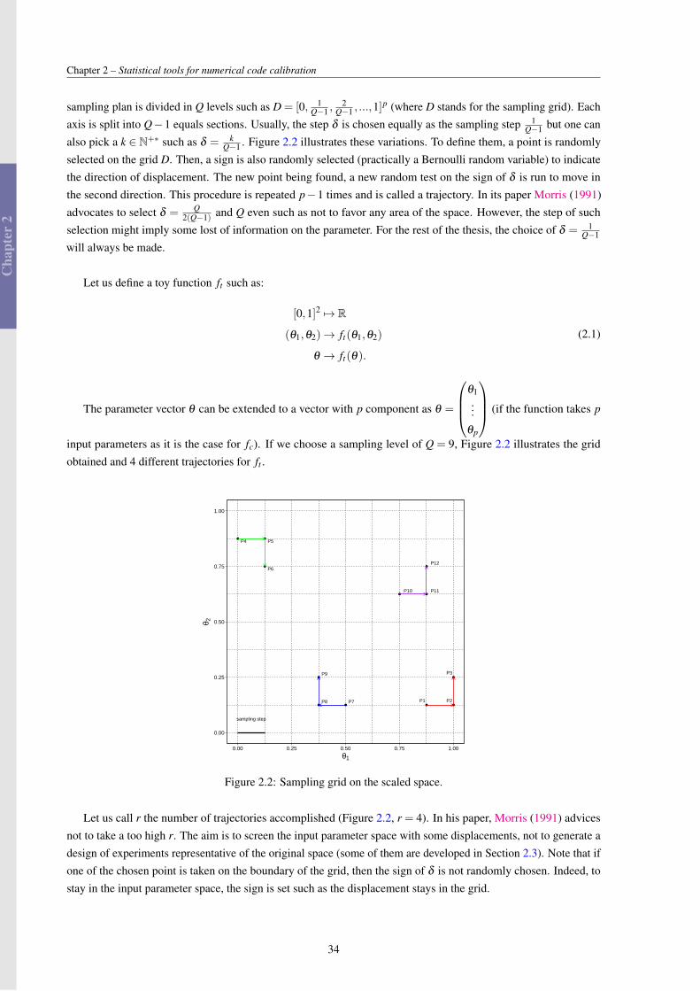
Cha

pter

2

Chapter 2 – Statistical tools for numerical code calibration

sampling plan is divided in Q levels such as D = [0, 1Q−1 ,

2Q−1 , ...,1]

p (where D stands for the sampling grid). Eachaxis is split into Q−1 equals sections. Usually, the step δ is chosen equally as the sampling step 1

Q−1 but one canalso pick a k ∈ N+∗ such as δ = k

Q−1 . Figure 2.2 illustrates these variations. To define them, a point is randomlyselected on the grid D. Then, a sign is also randomly selected (practically a Bernoulli random variable) to indicatethe direction of displacement. The new point being found, a new random test on the sign of δ is run to move inthe second direction. This procedure is repeated p−1 times and is called a trajectory. In its paper Morris (1991)advocates to select δ = Q

2(Q−1) and Q even such as not to favor any area of the space. However, the step of suchselection might imply some lost of information on the parameter. For the rest of the thesis, the choice of δ = 1

Q−1

will always be made.

Let us define a toy function ft such as:

[0,1]2 7→ R

(θ1,θ2)→ ft(θ1,θ2)

θ → ft(θ).

(2.1)

The parameter vector θ can be extended to a vector with p component as θ =

θ1...

θp

(if the function takes p

input parameters as it is the case for fc). If we choose a sampling level of Q = 9, Figure 2.2 illustrates the gridobtained and 4 different trajectories for ft .

P1 P2

P3

P4 P5

P6

P7P8

P9

P10 P11

P12

sampling step

0.00

0.25

0.50

0.75

1.00

0.00 0.25 0.50 0.75 1.00

θ1

θ 2

Figure 2.2: Sampling grid on the scaled space.

Let us call r the number of trajectories accomplished (Figure 2.2, r = 4). In his paper, Morris (1991) advicesnot to take a too high r. The aim is to screen the input parameter space with some displacements, not to generate adesign of experiments representative of the original space (some of them are developed in Section 2.3). Note that ifone of the chosen point is taken on the boundary of the grid, then the sign of δ is not randomly chosen. Indeed, tostay in the input parameter space, the sign is set such as the displacement stays in the grid.

34

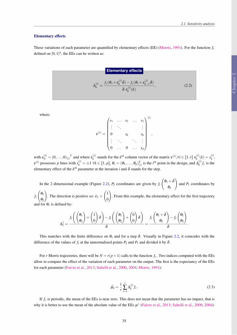
Cha

pter

2

2.1. Sensitivity analysis

Elementary effects

These variations of each parameter are quantified by elementary effects (EE) (Morris, 1991). For the function fc

defined on [0,1]p, the EEs can be written as:

∆(i)k =

fc(θ i + ε(i)k δ )− fc(θ i + ε

(i)k−1δ )

δ ε(i)k (k)

, (2.2)

Elementary effects

where:

ε(i) =

s1 . . . s1 . . . s1...

. . ....

0 sk sk...

. . . . . ....

0 . . . 0 . . . sp

(i)

,

with ε(i)0 = (0, . . . ,0)(i)T and where ε

(i)k stands for the kth column vector of the matrix ε(i),∀i ∈ J1,rK ε

(i)k (k) = s(i)k ,

ε(i) possesses p lines with s(i)k =±1 ∀k ∈ J1, pK, θ i = (θ1, . . . ,θp)T(i) is the ith point in the design, and ∆

(i)k fc is the

elementary effect of the kth parameter at the iteration i and δ stands for the step.

In the 2 dimensional example (Figure 2.2), P2 coordinates are given by ft

(θ1 +δ

θ2

)and P1 coordinates by

ft

(θ1

θ2

). The direction is positive so: ε1 =

(10

). From this example, the elementary effect for the first trajectory

and for θ1 is defined by:

∆11 =

ft

((θ1

θ2

)+

(10

)δ

)− ft

((θ1

θ2

)+

(00

)δ

)δ

=

ft

(θ1 +δ

θ2

)− ft

(θ1

θ2

)δ

.

This matches with the finite difference on θ1 and for a step δ . Visually in Figure 2.2, it coincides with thedifference of the values of ft at the unnormalized points P2 and P1 and divided it by δ .

For r Morris trajectories, there will be N = r(p+1) calls to the function fc. Two indices computed with the EEsallow to compare the effect of the variation of each parameter on the output. The first is the expectancy of the EEsfor each parameter (Faivre et al., 2013; Saltelli et al., 2000, 2004; Morris, 1991):

µk =1r

r

∑i=1

∆(i)k fc. (2.3)

If fc is periodic, the mean of the EEs is near zero. This does not mean that the parameter has no impact, that iswhy it is better to use the mean of the absolute value of the EEs µ∗ (Faivre et al., 2013; Saltelli et al., 2000, 2004):

35

Cha

pter

2

Chapter 2 – Statistical tools for numerical code calibration

µ∗k =1r

r

∑i=1| ∆(i)

k fc | . (2.4)

the estimated expectancy µ∗

The second index is the standard deviation of the EEs (Morris, 1991; Saltelli et al., 2004):

σk =

√1

r−1

r

∑i=1

(∆(i)k fc−µk)2. (2.5)

the estimated standard deviation σk

Indices µk, µ∗k and σ2k are Monte-Carlo estimators of respectively µk = EΘ[∆k fc(θ)], µ∗k = EΘ[

∣∣∆k fc(Θ)∣∣] and

σ2k = Var(∆k fc(Θ)) with Θ ∼Uni f [0, ..., k

Q−1 , ...,1p]. Thus, under regularity conditions of fc and its deriva-

tives, when δ → 0 these estimators converge toward∼µk =

∫[0,1]k

∂ fc∂θk

(θ)dθ ,∼µ∗k =

∫[0,1]k

∣∣ ∂ fc∂θk

∣∣(θ)dθ =∣∣∣∣ ∂ fc

∂θk

∣∣∣∣1 and

∼σ2

k =∫[0,1]k

∂ fc∂θk

2(θ)dθ −

∼µ2

k =∣∣∣∣ ∂ fc

∂θk

∣∣∣∣22−

∼µ2

k .

If the relation between the kth input parameter and the output is linear then the mean of the elementary effect isproportional to the intensity of the relation. The index σk, on the other hand, allows to detect interactions betweeninput parameters and is sensitive to the non-linearity of the output function of the kth input parameter (Faivre et al.,2013). A graph of the elementary effects can be display considering the x-axis as µ∗ and the y-axis as σ . Then,three areas appear:

• for low values of µ∗k and σk, the kth parameter is considered as having a negligible impact on the output,

• for hight values of µ∗k compared to σk, the kth parameter has a strong linear effect on the output,

• for hight values of σk the kth parameter has either a strong non-linear effect on the output and/or includes oneor several interactions with other ones.

One of the limits of this method is that we cannot differentiate parameters that have interaction with other onesfrom those which have a non-linear effect on the output (Faivre et al., 2013). To access this information anotherstudy has to be performed afterward. Computing the Sobol indices on the parameters left can be a solution (seeSection 2.1.2 for further details).

Morris function

In its paper, Morris (1991) introduced a test function of the method that allows to visualize the three areas. Thefunction takes 20 input parameters and is defined as:

Y = β0 +20

∑i=1

βiwi +20

∑i< j

βi, jwiw j +20

∑i< j<l

βi, j,lwiw jwl +20

∑i< j<l<s

βi, j,l,swiw jwlws, (2.6)

where,

wi =

2(1.1 Xi

Xi+0.1 −0.5) for i= 3, 5, 7,

2(Xi−0.5) otherwise.

36

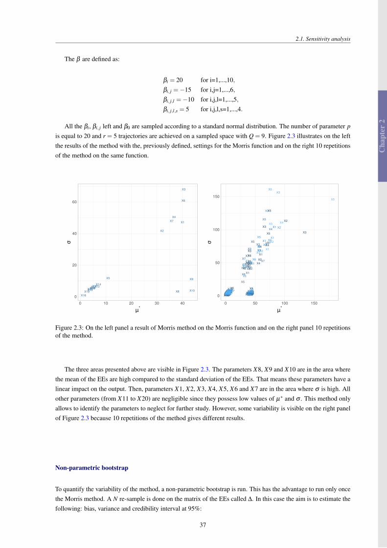
Cha

pter

2

2.1. Sensitivity analysis

The β are defined as:

βi = 20 for i=1,...,10,βi, j =−15 for i,j=1,...,6,βi, j,l =−10 for i,j,l=1,...,5,βi, j,l,s = 5 for i,j,l,s=1,...,4.

All the βi, βi, j left and β0 are sampled according to a standard normal distribution. The number of parameter p

is equal to 20 and r = 5 trajectories are achieved on a sampled space with Q = 9. Figure 2.3 illustrates on the leftthe results of the method with the, previously defined, settings for the Morris function and on the right 10 repetitionsof the method on the same function.

X1

X2

X3

X4

X5

X6

X7

X8

X9

X10X11X12

X13

X14X15

X16

X17X18

X19X20

0

20

40

60

0 10 20 30 40

μ*

σ

X1X2

X3

X4

X5

X6

X7

X8X9X10X11X12X13

X14X15X16

X17X18X19X20

X1X2

X3

X4

X5

X6

X7X8

X9X10X11

X12X13X14X15X16X17X18X19X20

X1

X2

X3

X4

X5

X6

X7

X8X9X10X11X12X13X14X15X16X17X18X19X20

X1

X2

X3

X4

X5

X6

X7X8X9X10

X11X12X13X14X15X16X17X18X19X20

X1

X2

X3

X4

X5

X6

X7

X8X9

X10X11X12X13

X14X15X16X17X18

X19X20

X1

X2X3

X4

X5

X6X7

X8X9X10X11X12

X13X14

X15X16X17X18X19X20

X1X2

X3

X4

X5X6

X7

X8X9X10X11X12X13X14X15X16X17X18X19X20

X1

X2

X3X4

X5

X6

X7

X8X9X10X11X12X13X14X15X16X17

X18X19X20

X1

X2

X3

X4

X5

X6

X7

X8X9X10X11X12X13X14X15X16X17X18X19X20

X1

X2

X3 X4

X5

X6X7

X8X9X10X11X12X13

X14X15X16X17X18X19X20

0

50

100

150

0 50 100 150

μ*

σ

Figure 2.3: On the left panel a result of Morris method on the Morris function and on the right panel 10 repetitionsof the method.

The three areas presented above are visible in Figure 2.3. The parameters X8, X9 and X10 are in the area wherethe mean of the EEs are high compared to the standard deviation of the EEs. That means these parameters have alinear impact on the output. Then, parameters X1, X2, X3, X4, X5, X6 and X7 are in the area where σ is high. Allother parameters (from X11 to X20) are negligible since they possess low values of µ∗ and σ . This method onlyallows to identify the parameters to neglect for further study. However, some variability is visible on the right panelof Figure 2.3 because 10 repetitions of the method gives different results.

Non-parametric bootstrap

To quantify the variability of the method, a non-parametric bootstrap is run. This has the advantage to run only oncethe Morris method. A N re-sample is done on the matrix of the EEs called ∆. In this case the aim is to estimate thefollowing: bias, variance and credibility interval at 95%:

37

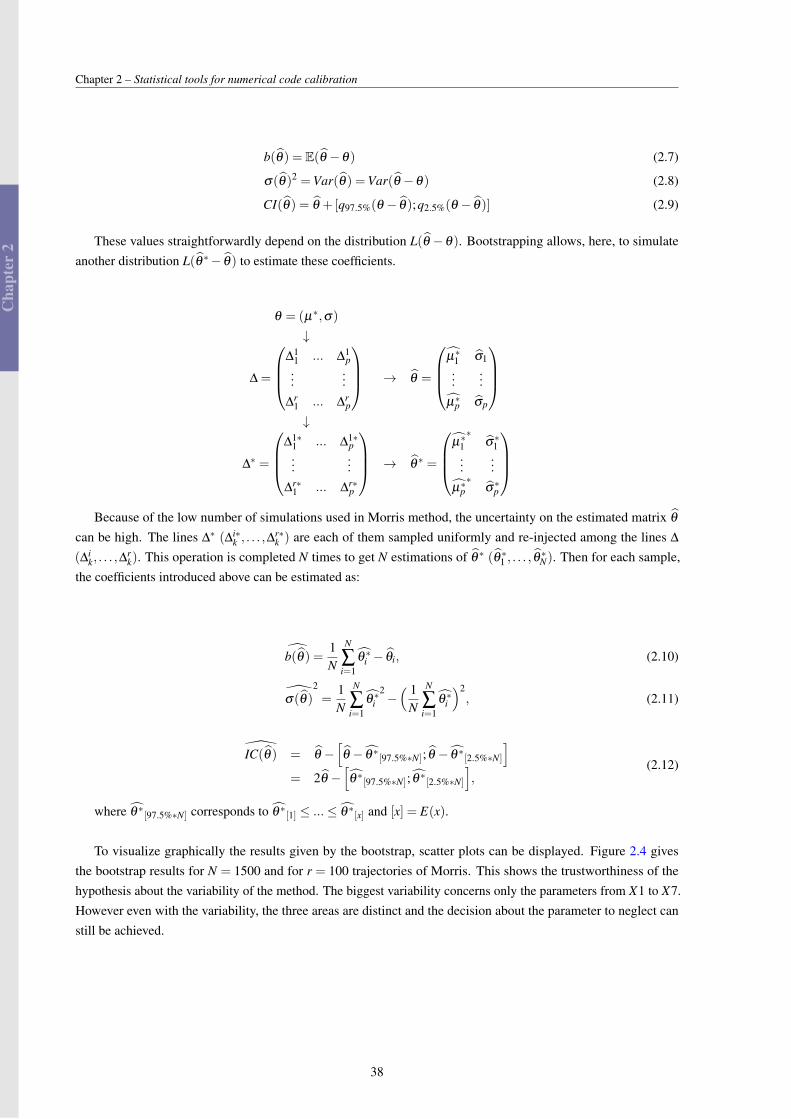
Cha

pter

2

Chapter 2 – Statistical tools for numerical code calibration

b(θ) = E(θ −θ) (2.7)

σ(θ)2 =Var(θ) =Var(θ −θ) (2.8)

CI(θ) = θ +[q97.5%(θ − θ);q2.5%(θ − θ)] (2.9)

These values straightforwardly depend on the distribution L(θ −θ). Bootstrapping allows, here, to simulateanother distribution L(θ ∗− θ) to estimate these coefficients.

θ = (µ∗,σ)

↓

∆ =

∆1

1 ... ∆1p

......

∆r1 ... ∆r

p

→ θ =

µ∗1 σ1...

...µ∗p σp

↓

∆∗ =

∆1∗

1 ... ∆1∗p

......

∆r∗1 ... ∆r∗

p

→ θ ∗ =

µ∗1∗

σ∗1...

...µ∗p∗

σ∗p

Because of the low number of simulations used in Morris method, the uncertainty on the estimated matrix θ

can be high. The lines ∆∗ (∆i∗k , . . . ,∆

r∗k ) are each of them sampled uniformly and re-injected among the lines ∆

(∆ik, . . . ,∆

rk). This operation is completed N times to get N estimations of θ ∗ (θ ∗1 , . . . , θ

∗N). Then for each sample,

the coefficients introduced above can be estimated as:

b(θ) =1N

N

∑i=1

θ ∗i − θi, (2.10)

σ(θ)2=

1N

N

∑i=1

θ ∗i2−( 1

N

N

∑i=1

θ ∗i

)2, (2.11)

IC(θ) = θ −[θ − θ ∗[97.5%∗N]; θ − θ ∗[2.5%∗N]

]= 2θ −

[θ ∗[97.5%∗N]; θ ∗[2.5%∗N]

],

(2.12)

where θ ∗[97.5%∗N] corresponds to θ ∗[1] ≤ ...≤ θ ∗[x] and [x] = E(x).

To visualize graphically the results given by the bootstrap, scatter plots can be displayed. Figure 2.4 givesthe bootstrap results for N = 1500 and for r = 100 trajectories of Morris. This shows the trustworthiness of thehypothesis about the variability of the method. The biggest variability concerns only the parameters from X1 to X7.However even with the variability, the three areas are distinct and the decision about the parameter to neglect canstill be achieved.

38

Cha

pter

2

2.1. Sensitivity analysis

X1X2

X3

X4

X5

X6

X7

X8X9X10X11X12X13X14X15X16X17X18X19X20

X1X2

X3

X4

X5

X6

X7

X8X9X10X11X12X13X14X15X16X17X18X19X20

0

50

100

0 20 40 60 80

μ*

σ

Figure 2.4: Scatter plot of the Morris indices given by the 1500 iterations bootstrap.

2.1.2 Sobol indices

The Morris method only allows to detect parameters that have no impact on the output and hence can be negligible.However to get more information on which parameter has the more influence on the output, another method needs tobe applied. Sensitivity index based on a measure of importance can be used and in this section, the variance-basedsensitivity analysis is presented. This method is also called Sobol method and uses the variance as the measure ofinfluence of the output to get sensitivity index.

First order sensitivity index

Sobol method has been introduced by Sobol’ (1990) and, as it is the case for the Morris method, the parameter inputspace is normalized between 0 and 1. It means that the space Ω is the k sized hypercube. From Fourier Haar’s series,Sobol, in a previous work, had proposed a decomposition of the function fc such as:

fc(θ1, . . . ,θk) = fc0 +k

∑i=1

fci(θi)+ ∑1≤i< j≤k

fci j(θi,θ j)+ · · ·+ fc1,2,...,k(θ1, . . . ,θk). (2.13)

For Equation (2.13) to make sense, fc0 must be constant and the integral of each part of the sum must be null:

∫ 1

0fci1 ,...,is

(θi1 , . . . ,θis)dθik = 0 if 1≤ k ≤ s. (2.14)

The consequence of Equation (2.13) and Equation (2.14) is that all the parts of the sum are orthogonal. So, if(i1, . . . , is) 6= ( j1, . . . , jl) then: ∫

Ω

fci1 ,...,isfc j1 ,..., js

dθ = 0. (2.15)

Sobol shows, in its article Sobol (1993), that the decomposition given in Equation (2.13) is unique and all theterms can be evaluated thanks to multidimensional integrals:

fci(θi) =− fc0 +∫ 1

0· · ·∫ 1

0fc(θ)dθ∼i,

fci j(θi,θ j) =− fc0 − fci(θi)− fc j(θ j)+∫ 1

0· · ·∫ 1

0fc(θ)dθ∼(i j).

where dθ∼i and dθ∼(i j) stands for the integrations over the whole domain Ω without (respectively) θi and, θi

39

Cha

pter

2

Chapter 2 – Statistical tools for numerical code calibration

and θ j. Total variance D of fc(θ) can be expressed by:

D =∫

Ωkf 2c (θ)dθ− f 2

c0. (2.16)

In a similar way and thank to the decomposition introduced in Equation (2.13), partial variances can be writtenas:

Di1,...,is =∫ 1

0· · ·∫ 1

0f 2ci1 ,...,is

(θi1 , . . . ,θis)dθi1 . . .dθis , (2.17)

where 1≤ i1 < · · ·< is ≤ k and s = 1, . . . ,k. When the square of Equation (2.13) is taken and then integratedover Ωk, the total variance is written:

D =k

∑i=1

Di + ∑1≤i< j≤k

Di j + · · ·+D1,2,...,k. (2.18)

The first index in the Sobol method is called the first order Sobol index and is defined as:

Si =Di

D. (2.19)

First order Sobol’s index

The first order Sobol’s index is Si for the parameter θi. This index allows to quantify the principal effects of thisparameter on the variance of the output. The formula Si =

Var[Y |θi]Var[Y ] is, here, found back. The Si j for i 6= j are called

second order index and allow to quantify the interactions between θi and θ j that are not taken into account in Si. IfEquation (2.18) is divided by D and replaced by Sobol’s index defined in Equation (2.19), then:

k

∑i=1

Si + ∑1≤i< j≤k

Si j + · · ·+S1,2,...,k = 1. (2.20)

Total effect index

Total effect index or total sensitivity index (TSI) are defined as the sum of the all the indices encompassing thestudied parameter. This definition can be rewritten as:

T S(i) = ∑I⊆i

Si. (2.21)

Total sensitivity index

In a 3-dimensional toy example, the TSI of the parameter θ1 is given by T S(1) = S1 +S12 +S13 +S123 where S1

is the first-order index of the parameter θ1 on the output yc, S12 and S13 are the second order index which arequantifying the interactions of θ1 with θ2 and θ3, and S123 the third order index. If T S(i) ≈ Si, that means onlythe first-order index has a significant impact on the output and the superior order indices are then negligible. It iscommon to compute the first order index and the total index to check if interactions are present.

Compared to the Morris method, Sobol indices allow to visualize interactions between parameters. However,the computation of the first order and the total effect Sobol’s indices are performed with a design D. To have aglobal study on the overall impact, for the range ofD, the analysis has to be run for each θ inD which is really

40

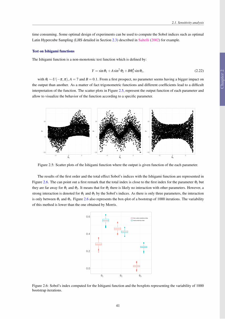
Cha

pter

2

2.1. Sensitivity analysis

time consuming. Some optimal design of experiments can be used to compute the Sobol indices such as optimalLatin Hypercube Sampling (LHS detailed in Section 2.3) described in Saltelli (2002) for example.

Test on Ishigami functions

The Ishigami function is a non-monotonic test function which is defined by:

Y = sinθ1 +Asin2θ2 +Bθ

43 sinθ1, (2.22)

with θi ∼U(−π,π), A = 7 and B = 0.1. From a first prospect, no parameter seems having a bigger impact onthe output than another. As a matter of fact trigonometric functions and different coefficients lead to a difficultinterpretation of the function. The scatter plots in Figure 2.5, represent the output function of each parameter andallow to visualize the behavior of the function according to a specific parameter.

−10

0

10

−2 0 2θ1

y

−10

0

10

−2 0 2θ2

y

−10

0

10

−2 0 2θ3

y

Figure 2.5: Scatter plots of the Ishigami function where the output is given function of the each parameter.

The results of the first order and the total effect Sobol’s indices with the Ishigami function are represented inFigure 2.6. The can point out a first remark that the total index is close to the first index for the parameter θ2 butthey are far away for θ1 and θ3. It means that for θ2 there is likely no interaction with other parameters. However, astrong interaction is denoted for θ1 and θ3 by the Sobol’s indices. As there is only three parameters, the interactionis only between θ1 and θ3. Figure 2.6 also represents the box-plot of a bootstrap of 1000 iterations. The variabilityof this method is lower than the one obtained by Morris.

0.0

0.2

0.4

0.6

θ1 θ2 θ3

First−order sensitivity index

Total sensitivity index

Figure 2.6: Sobol’s index computed for the Ishigami function and the boxplots representing the variability of 1000bootstrap iterations.

41

Cha

pter

2

Chapter 2 – Statistical tools for numerical code calibration

2.2 Kriging / Gaussian processes

In mining engineering, predicting the content at site, knowing the content of neighbor sites by a Gaussian processcomes from Krige (1951) and is called Kriging. Then Matheron, in Matheron (1963), has proposed the Krigingmethod to model spatial data in geostatistics (Cressie and Noel, 1993; Stein, 2012). This is Sacks et al. (1989) thathave used this formal modeling as surrogate in a numerical experiment framework. More than a surrogate, this kindof modeling brings also an indicator of the uncertainty according to a prediction of the surrogate at a given point.This section will focus, first, on the general framework of the Gaussian process and in a second part on the mainparameter estimation methods. Then, on a third part some general covariance functions, used to depict correlationbetween nearby sites, are developed. To optimize the design of experiments regarding the quality of the Gaussianprocess, some Gaussian process-based optimization method have been developed and one of them, named EfficientGlobal Optimization (EGO), is presented in the fourth part.

2.2.1 General framework

Let us consider a probability space (Ω,F ,π) where Ω stands for a sample space, F a σ -algebra on Ω and π aprobability on F . A stochastic process X is a family as Xt ; t ∈ T where T ⊂ Rd . It is said that the aleatoryprocess is indexed by t. At t fixed, the application Xt : Ω→R is a random variable. At ω ∈Ω fixed, the applicationt→ Xt(ω) is a trajectory of the stochastic process.

For t1 ∈T , . . . , tn ∈T , the probability distribution of the random vector (Xt1 , . . . ,Xtn) is called finite-dimensionaldistributions of the stochastic process Xtt∈T . Hence, the probability distribution of an aleatory process is deter-mined by its finite-dimensional distributions. Kolmogorov’s theorem guaranties the existence of such a stochasticprocess if a suitably collection of coherent finite-dimensional distributions is provided.

A random vector Z such as Z = (Z1, . . . ,Zn) is Gaussian if ∀λ1, . . . ,λn ∈ R the random variable ∑ni=1 λiZi

is Gaussian. The distribution of Z is straightforwardly determined by its two first moments: the mean µ =

(E[Z1], . . . ,E[Zn]) and the variance covariance matrix Σ = cov(Zi,Z j)1≤i, j≤n. When Σ is positive definite, Z has aprobability density defined by Equation (2.23).

π(z) =|Σ|−1/2

(2π)n/2 exp− 1

2(z−µ)T Σ−1(z−µ)

. (2.23)

Let us consider two Gaussian vectors called U1 and U2 such as:(U1

U2

)∼N

((µ1

µ2

),

(Σ1,1 Σ1,2

Σ2,1 Σ2,2

)).

The conditional distribution U2|U1 is also Gaussian (Equation (2.24)). This property is the base of Krigingwhen a Gaussian process is used as a surrogate of a function.

U2|U1 ∼N(µ2 +Σ2,1Σ−1

1,1(U1−µ1),Σ2,2−Σ2,1Σ−11,1Σ1,2

). (2.24)

Conditional distribution

A stochastic process Xtt∈T is a Gaussian process if each of its finite-dimensional distributions are Gaussian.Let us introduce the mean function such as m : t ∈ T → m(t) = E[Xt ] and the correlation function such asK : (t, t ′) ∈T ×T → K(t, t ′) = corr(Xt ,Xt ′) (as well noted r(t, t ′) in the thesis). A Gaussian process with a certainvariance noted σ2 will be defined as Equation (2.25).

42

Cha

pter

2

2.2. Kriging / Gaussian processes

X(.)∼PG (m(.),σ2K(., .)). (2.25)

Gaussian processes are used in this thesis in two cases. In the fist one, fc is a code function long to run and theGaussian process emulates its behaviour. Then the Gaussian process is the surrogate of the code. The second case iswhen we want to model the error made by the code (called code error or discrepancy). For the former, we want tocreate a surrogate fc of a deterministic function fc. Let us define this function to emulate fc such as:

fc : Q ⊂ Rp→ R

θ 7→ fc(θ).(2.26)

Following previous statement, fc is a realization of a Gaussian process. In a Bayesian framework, the Gaussianprocess is a “functional” a priori on fc (Currin et al., 1991). The natural idea of the Gaussian process emulation isto use known evaluations of fc at some selected points from a design of experiments D, and access information ofthe evaluation of fc at some point θ0 where θ0 6∈ D. The modeling with a Gaussian process of the function fc canbe written as:

fc(•)∼PG (H(•)Tβ,σ2Kψ(•,•)), (2.27)

where β is a parameter vector such as β = (β1, . . . ,βp), σ2 and ψ respectively stands for the variance and thecorrelation length of the covariance function cσ ,ψ(•,•) = c(•,•) = σ2Kψ(•,•) andH(•) the matrix of regressors.The covariance function is defined as:

(θ,θ′) ∈Q×Q, c(θ,θ′) = σ2Kψ(θ,θ′). (2.28)

Covariance function

Equation (2.27) can also be written as:

θ ∈Q, fc(θ) =H(θ)Tβ+Z(θ), (2.29)

Gaussian process

where Z(θ) represents a centered Gaussian process characterized by its covariance function c(Z(θ),Z(θ′) =

σ2Kψ(θ,θ′). Let us consider a toy function ft we try to emulated by a Gaussian process with 5 points in the designof experiments:

ft : [0,1]→ R

θ 7→ y = (6θ −2)2sin(11θ −4) .(2.30)

To visualize the impact of parameter values, some Gaussian process realizations are performed with differentvalues of σ2 and ψ. The results are displayed in Figure 2.7 and allows to note that these parameters values impactsthe Gaussian process quality.

Usually β, σ2 and ψ are unknown. Some modeling consider them as determined values but, practically, theyare estimated upstream with methods described in Section 2.2.2. They also can be considered as unknown duringthe Gaussian process modeling with their associated uncertainty encompassed. However, this could lead to complex

43

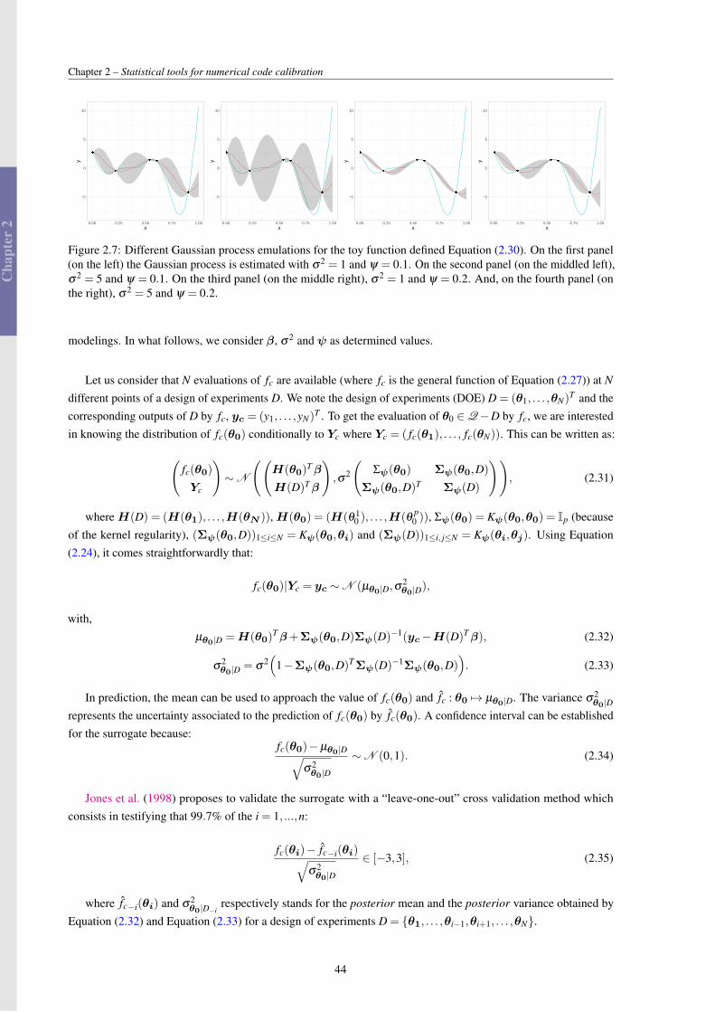
Cha

pter

2

Chapter 2 – Statistical tools for numerical code calibration

−5

0

5

10

0.00 0.25 0.50 0.75 1.00x

y

−5

0

5

10

0.00 0.25 0.50 0.75 1.00x

y

−5

0

5

10

0.00 0.25 0.50 0.75 1.00x

y

−5

0

5

10

0.00 0.25 0.50 0.75 1.00x

y

Figure 2.7: Different Gaussian process emulations for the toy function defined Equation (2.30). On the first panel(on the left) the Gaussian process is estimated with σ2 = 1 and ψ = 0.1. On the second panel (on the middled left),σ2 = 5 and ψ = 0.1. On the third panel (on the middle right), σ2 = 1 and ψ = 0.2. And, on the fourth panel (onthe right), σ2 = 5 and ψ = 0.2.

modelings. In what follows, we consider β, σ2 and ψ as determined values.

Let us consider that N evaluations of fc are available (where fc is the general function of Equation (2.27)) at N

different points of a design of experiments D. We note the design of experiments (DOE) D = (θ1, . . . ,θN)T and the

corresponding outputs of D by fc, yc = (y1, . . . ,yN)T . To get the evaluation of θ0 ∈Q−D by fc, we are interested

in knowing the distribution of fc(θ0) conditionally to Yc where Yc = ( fc(θ1), . . . , fc(θN)). This can be written as:

(fc(θ0)

Yc

)∼N

((H(θ0)

Tβ

H(D)Tβ

),σ2

(Σψ(θ0) Σψ(θ0,D)

Σψ(θ0,D)T Σψ(D)

)), (2.31)

whereH(D) = (H(θ1), . . . ,H(θN )),H(θ0) = (H(θ 10 ), . . . ,H(θ p

0 )), Σψ(θ0) = Kψ(θ0,θ0) = Ip (becauseof the kernel regularity), (Σψ(θ0,D))1≤i≤N = Kψ(θ0,θi) and (Σψ(D))1≤i, j≤N = Kψ(θi,θj). Using Equation(2.24), it comes straightforwardly that:

fc(θ0)|Yc = yc ∼N (µθ0|D,σ2θ0|D),

with,µθ0|D =H(θ0)

Tβ+Σψ(θ0,D)Σψ(D)−1(yc−H(D)Tβ), (2.32)

σ2θ0|D = σ

2(

1−Σψ(θ0,D)T Σψ(D)−1Σψ(θ0,D)). (2.33)

In prediction, the mean can be used to approach the value of fc(θ0) and fc : θ0 7→ µθ0|D. The variance σ2θ0|D

represents the uncertainty associated to the prediction of fc(θ0) by fc(θ0). A confidence interval can be establishedfor the surrogate because:

fc(θ0)−µθ0|D√σ2θ0|D

∼N (0,1). (2.34)

Jones et al. (1998) proposes to validate the surrogate with a “leave-one-out” cross validation method whichconsists in testifying that 99.7% of the i = 1, ...,n:

fc(θi)− fc−i(θi)√σ2θ0|D

∈ [−3,3], (2.35)

where fc−i(θi) and σ2θ0|D−i

respectively stands for the posterior mean and the posterior variance obtained byEquation (2.32) and Equation (2.33) for a design of experiments D = θ1, . . . ,θi−1,θi+1, . . . ,θN.

44

Cha

pter

2

2.2. Kriging / Gaussian processes

The predictor fc(θ0) is the Best Linear Predictor (BLP) if it minimizes the following Mean Square Error (MSE):

MSE(θ0) = E[( fc(θ0)− fc(θ0))2]. (2.36)

With β, σ2 and ψ fixed, and under hypotheses of Equation (2.27), the best linear predictor of fc(θ0) is:

θ0 7→H(θ0)Tβ+Σψ(θ0,D)Σψ(D)−1(yc−H(D)Tβ). (2.37)

Best linear predictor

This predictor is unbiased and its mean square error is equal to MSE(θ0) = σ2θ0|D. If the evaluated point is

taken in the original design D (i.e. θ0 = θi ∈Q), then µ2θ0|D = yi and σ2

θ0|D = 0.

2.2.2 Parameter estimation

Maximum likelihood estimates

Practically, β is unknown, and, to estimate it, a generalized least square method is commonly applied whichcorresponds to the maximum likelihood of Equation (2.23). This gives:

β = (H(D)T Σψ(D)−1H(D))−1H(D)T Σψ(D)−1yc. (2.38)

β prediction

The predictor given Equation (2.37) can be rewritten as:

fc(θ0) =H(θ0)T β+Σψ(θ0,D)Σψ(D)−1(yc−H(D)T β), (2.39)

and its mean square error is:

Var( fc(θ0)) = E( fc(θ0)− fc(θ0))2

= σ2(1+u(θ0)

T (H(D)TΣψ(D)−1H(D))−1u(θ0)−Σψ(θ0,D)T

Σψ(D)−1Σψ(θ0,D),

(2.40)

where u(θ0) =H(θ0)T Σψ(D)−1Σψ(θ0,D)−H(θ0). This prediction mean square error is applied when β is not

fixed. If it is fixed the prediction mean square error is given Equation (2.33) but in both cases the predictor meansquare error corresponds to the predictor variance since it is unbiased. If we consider σ2 and β as unknown, thecovariance matrix known, then fc(θ0) is the Best Linear Unbiased Predictor (BLUP) of fc(θ0).

To estimate the parameter σ2, that only intervenes in the calculation of the root mean square error, a maximumlikelihood can be applied and:

σ2 =

1N(Yc−H(D)β)T

Σψ(D)−1(Yc−H(D)β). (2.41)

σ2 prediction

45

Cha

pter

2

Chapter 2 – Statistical tools for numerical code calibration

Then, the parameter ψ is estimated after having plugged β and σ2 in the likelihood and getting the maximum.After parameter plugging, the opposite log-likelihood can be written as:

L (Yc;ψ) ∝ Nlog(σ2)+ log(|Σψ(D)|), (2.42)

and, ψ = argminψ

L (Yc;ψ).

The resulting predictor

fc(θ0) =H(θ0)T β+Σψ(θ0,D)T

Σψ(D)(Yc−H(D)β) (2.43)

is called EBLUP (Empirical Best Linear Unbiased Predictor) although it is neither linear nor unbiased. Maximumlikelihood estimation, and “plug-in” techniques under estimate the prediction variance (Handcock and Stein, 1993;Helbert et al., 2009) and does not take into account any uncertainty affecting the parameters β, σ2 and ψ.

Bayesian estimation

In this section we focus on Bayesian estimation of σ2 and β. We will consider a three level hierarchical model,in the sense of Robert (2007), in where the lowest level only deals with the parameter β. At the second level, theparameter σ2 controls the distribution of β and at the top level, the parameter ψ controls the distribution of σ2 andβ. Note that the estimation of σ2 causes the loss of normality a posteriori. The prior density of (β,σ2) can bewritten:

π(β,σ2) = π(β|σ2)π(σ2). (2.44)

In this section we will work with the four configurations of priors present in Santner et al. (2013); Le Gratiet(2013):

1. σ2 ∼I G (α,γ) and β|σ2 ∼N (b0,σ2V0)

2. π(σ2) ∝1

σ2 and β|σ2 ∼N (b0,σ2V0)

3. σ2 ∼I G (α,γ) and π(β|σ2) ∝ 1

4. π(σ2) ∝1

σ2 and π(β|σ2) ∝ 1

The first case is the more common in Bayesian Kriging because both priors are conjugate to a normal likelihoodand the posterior density can, explicitly, be written. In the presented configurations, I G (α,γ) stands for the inverseGamma distribution

π(x) =γα

Γ(α)

e−γ/x

xα+1 1x>0.

The computation of the posterior density can be done for each cases and for ψ fixed. In each cases, the posterior

can be expressed as π(β|yc,σ2)∼N (νΣ,Σ) with:

Σ−1 =

(HT Σψ(D)H+V0)/σ2 for the cases (1) and (2),

(HT Σψ(D)H)/σ2 for the cases (3) and (4),(2.45)

and,

ν =

(HT Σψ(D)yc+V0b0)/σ2 for the cases (1) and (2),

(HT Σψ(D)yc)/σ2 for the cases (3) and (4).(2.46)

46

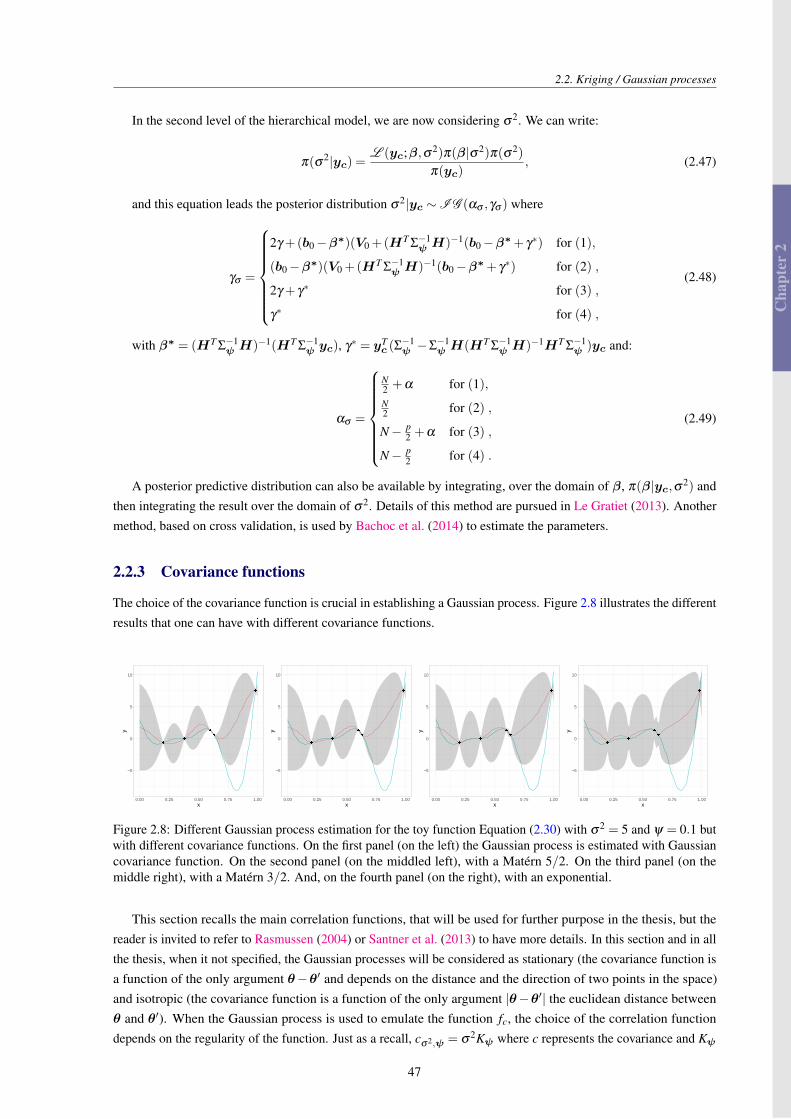
Cha

pter

2

2.2. Kriging / Gaussian processes

In the second level of the hierarchical model, we are now considering σ2. We can write:

π(σ2|yc) =L (yc;β,σ2)π(β|σ2)π(σ2)

π(yc), (2.47)

and this equation leads the posterior distribution σ2|yc ∼I G (ασ ,γσ ) where

γσ =

2γ +(b0−β∗)(V0 +(HT Σ−1ψ H)−1(b0−β∗+ γ∗) for (1),

(b0−β∗)(V0 +(HT Σ−1ψ H)−1(b0−β∗+ γ∗) for (2) ,

2γ + γ∗ for (3) ,

γ∗ for (4) ,

(2.48)

with β∗ = (HT Σ−1ψ H)−1(HT Σ

−1ψ yc), γ∗ = yT

c (Σ−1ψ −Σ

−1ψ H(HT Σ

−1ψ H)−1HT Σ

−1ψ )yc and:

ασ =

N2 +α for (1),N2 for (2) ,

N− p2 +α for (3) ,

N− p2 for (4) .

(2.49)

A posterior predictive distribution can also be available by integrating, over the domain of β, π(β|yc,σ2) andthen integrating the result over the domain of σ2. Details of this method are pursued in Le Gratiet (2013). Anothermethod, based on cross validation, is used by Bachoc et al. (2014) to estimate the parameters.

2.2.3 Covariance functions

The choice of the covariance function is crucial in establishing a Gaussian process. Figure 2.8 illustrates the differentresults that one can have with different covariance functions.

−5

0

5

10

0.00 0.25 0.50 0.75 1.00x

y

−5

0

5

10

0.00 0.25 0.50 0.75 1.00x

y

−5

0

5

10

0.00 0.25 0.50 0.75 1.00x

y

−5

0

5

10

0.00 0.25 0.50 0.75 1.00x

y

Figure 2.8: Different Gaussian process estimation for the toy function Equation (2.30) with σ2 = 5 and ψ = 0.1 butwith different covariance functions. On the first panel (on the left) the Gaussian process is estimated with Gaussiancovariance function. On the second panel (on the middled left), with a Matérn 5/2. On the third panel (on themiddle right), with a Matérn 3/2. And, on the fourth panel (on the right), with an exponential.

This section recalls the main correlation functions, that will be used for further purpose in the thesis, but thereader is invited to refer to Rasmussen (2004) or Santner et al. (2013) to have more details. In this section and in allthe thesis, when it not specified, the Gaussian processes will be considered as stationary (the covariance function isa function of the only argument θ−θ′ and depends on the distance and the direction of two points in the space)and isotropic (the covariance function is a function of the only argument |θ−θ′| the euclidean distance betweenθ and θ′). When the Gaussian process is used to emulate the function fc, the choice of the correlation functiondepends on the regularity of the function. Just as a recall, cσ2,ψ = σ2Kψ where c represents the covariance and Kψ

47

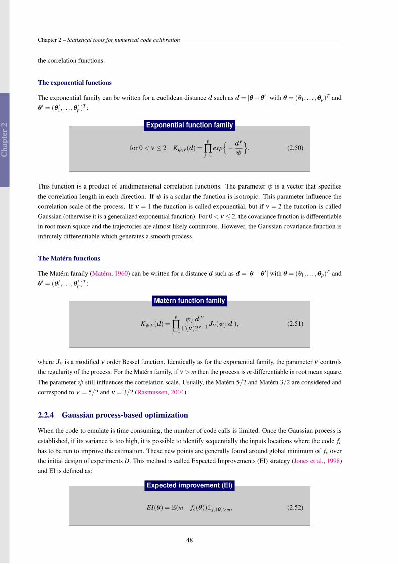
Cha

pter

2

Chapter 2 – Statistical tools for numerical code calibration

the correlation functions.

The exponential functions

The exponential family can be written for a euclidean distance d such as d= |θ−θ′| with θ = (θ1, . . . ,θp)T and

θ′ = (θ ′1, . . . ,θ′p)

T :

for 0 < ν ≤ 2 Kψ,ν(d) =p

∏j=1

exp− d

ν

ψ

. (2.50)

Exponential function family

This function is a product of unidimensional correlation functions. The parameter ψ is a vector that specifiesthe correlation length in each direction. If ψ is a scalar the function is isotropic. This parameter influence thecorrelation scale of the process. If ν = 1 the function is called exponential, but if ν = 2 the function is calledGaussian (otherwise it is a generalized exponential function). For 0 < ν ≤ 2, the covariance function is differentiablein root mean square and the trajectories are almost likely continuous. However, the Gaussian covariance function isinfinitely differentiable which generates a smooth process.

The Matérn functions

The Matérn family (Matérn, 1960) can be written for a distance d such as d= |θ−θ′| with θ = (θ1, . . . ,θp)T and

θ′ = (θ ′1, . . . ,θ′p)

T :

Kψ,ν(d) =p

∏j=1

ψ j|d|ν

Γ(ν)2ν−1Jν(ψ j|d|), (2.51)

Matérn function family

where Jν is a modified ν order Bessel function. Identically as for the exponential family, the parameter ν controlsthe regularity of the process. For the Matérn family, if ν > m then the process is m differentiable in root mean square.The parameter ψ still influences the correlation scale. Usually, the Matérn 5/2 and Matérn 3/2 are considered andcorrespond to ν = 5/2 and ν = 3/2 (Rasmussen, 2004).

2.2.4 Gaussian process-based optimization

When the code to emulate is time consuming, the number of code calls is limited. Once the Gaussian process isestablished, if its variance is too high, it is possible to identify sequentially the inputs locations where the code fc

has to be run to improve the estimation. These new points are generally found around global minimum of fc overthe initial design of experiments D. This method is called Expected Improvements (EI) strategy (Jones et al., 1998)and EI is defined as:

EI(θ) = E(m− fc(θ))1 fc(θ)>m, (2.52)

Expected improvement (EI)

48

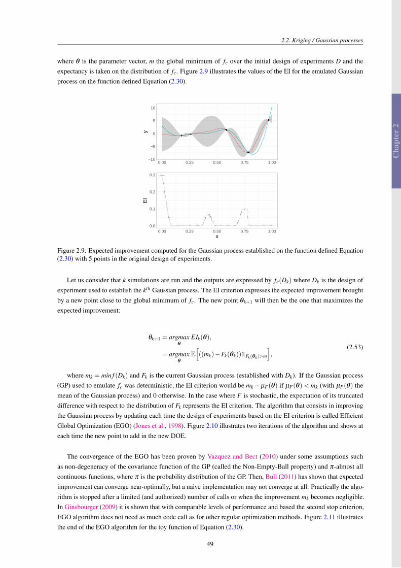
Cha

pter

2

2.2. Kriging / Gaussian processes

where θ is the parameter vector, m the global minimum of fc over the initial design of experiments D and theexpectancy is taken on the distribution of fc. Figure 2.9 illustrates the values of the EI for the emulated Gaussianprocess on the function defined Equation (2.30).

−10

−5

0

5

10

0.00 0.25 0.50 0.75 1.00

y

0.0

0.1

0.2

0.3

0.00 0.25 0.50 0.75 1.00x

EI

Figure 2.9: Expected improvement computed for the Gaussian process established on the function defined Equation(2.30) with 5 points in the original design of experiments.

Let us consider that k simulations are run and the outputs are expressed by fc(Dk) where Dk is the design ofexperiment used to establish the kth Gaussian process. The EI criterion expresses the expected improvement broughtby a new point close to the global minimum of fc. The new point θk+1 will then be the one that maximizes theexpected improvement:

θk+1 = argmaxθ

EIk(θ),

= argmaxθ

E[((mk)−Fk(θk))1Fk(θk)>m

],

(2.53)

where mk = min f (Dk) and Fk is the current Gaussian process (established with Dk). If the Gaussian process(GP) used to emulate fc was deterministic, the EI criterion would be mk−µF(θ) if µF(θ)< mk (with µF(θ) themean of the Gaussian process) and 0 otherwise. In the case where F is stochastic, the expectation of its truncateddifference with respect to the distribution of Fk represents the EI criterion. The algorithm that consists in improvingthe Gaussian process by updating each time the design of experiments based on the EI criterion is called EfficientGlobal Optimization (EGO) (Jones et al., 1998). Figure 2.10 illustrates two iterations of the algorithm and shows ateach time the new point to add in the new DOE.

The convergence of the EGO has been proven by Vazquez and Bect (2010) under some assumptions suchas non-degeneracy of the covariance function of the GP (called the Non-Empty-Ball property) and π-almost allcontinuous functions, where π is the probability distribution of the GP. Then, Bull (2011) has shown that expectedimprovement can converge near-optimally, but a naive implementation may not converge at all. Practically the algo-rithm is stopped after a limited (and authorized) number of calls or when the improvement mk becomes negligible.In Ginsbourger (2009) it is shown that with comparable levels of performance and based the second stop criterion,EGO algorithm does not need as much code call as for other regular optimization methods. Figure 2.11 illustratesthe end of the EGO algorithm for the toy function of Equation (2.30).

49

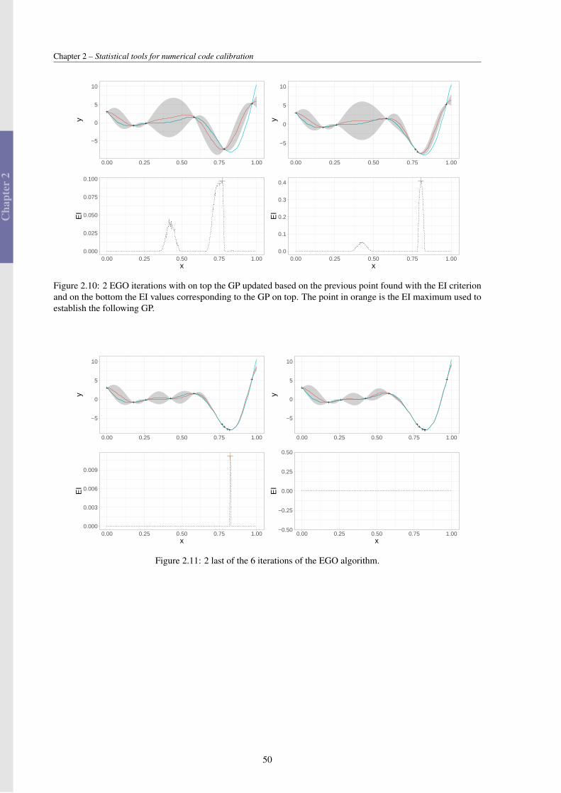
Cha

pter

2

Chapter 2 – Statistical tools for numerical code calibration

−5

0

5

10

0.00 0.25 0.50 0.75 1.00

y

0.000

0.025

0.050

0.075

0.100

0.00 0.25 0.50 0.75 1.00x

EI

−5

0

5

10

0.00 0.25 0.50 0.75 1.00

y

0.0

0.1

0.2

0.3

0.4

0.00 0.25 0.50 0.75 1.00x

EI

Figure 2.10: 2 EGO iterations with on top the GP updated based on the previous point found with the EI criterionand on the bottom the EI values corresponding to the GP on top. The point in orange is the EI maximum used toestablish the following GP.

−5

0

5

10

0.00 0.25 0.50 0.75 1.00

y

0.000

0.003

0.006

0.009

0.00 0.25 0.50 0.75 1.00x

EI

−5

0

5

10

0.00 0.25 0.50 0.75 1.00

y

−0.50

−0.25

0.00

0.25

0.50

0.00 0.25 0.50 0.75 1.00x

EI

Figure 2.11: 2 last of the 6 iterations of the EGO algorithm.

50

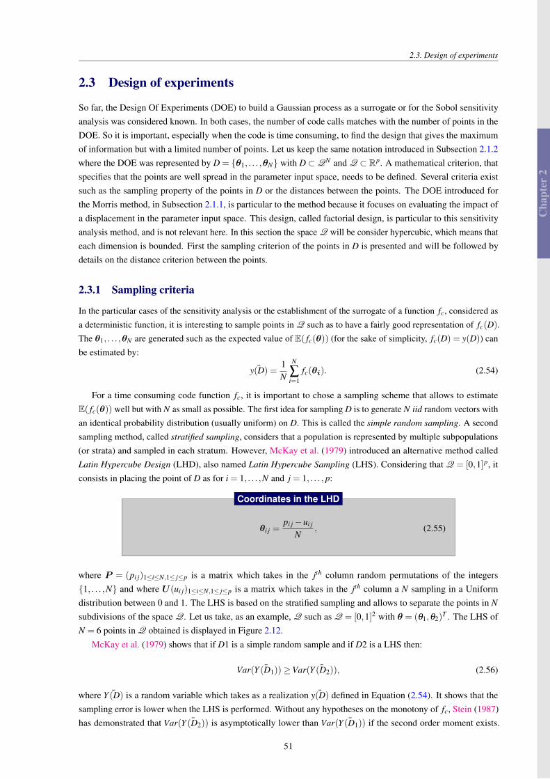
Cha

pter

2

2.3. Design of experiments

2.3 Design of experiments

So far, the Design Of Experiments (DOE) to build a Gaussian process as a surrogate or for the Sobol sensitivityanalysis was considered known. In both cases, the number of code calls matches with the number of points in theDOE. So it is important, especially when the code is time consuming, to find the design that gives the maximumof information but with a limited number of points. Let us keep the same notation introduced in Subsection 2.1.2where the DOE was represented by D = θ1, . . . ,θN with D⊂QN and Q ⊂ Rp. A mathematical criterion, thatspecifies that the points are well spread in the parameter input space, needs to be defined. Several criteria existsuch as the sampling property of the points in D or the distances between the points. The DOE introduced forthe Morris method, in Subsection 2.1.1, is particular to the method because it focuses on evaluating the impact ofa displacement in the parameter input space. This design, called factorial design, is particular to this sensitivityanalysis method, and is not relevant here. In this section the space Q will be consider hypercubic, which means thateach dimension is bounded. First the sampling criterion of the points in D is presented and will be followed bydetails on the distance criterion between the points.

2.3.1 Sampling criteria

In the particular cases of the sensitivity analysis or the establishment of the surrogate of a function fc, considered asa deterministic function, it is interesting to sample points in Q such as to have a fairly good representation of fc(D).The θ1, . . . ,θN are generated such as the expected value of E( fc(θ)) (for the sake of simplicity, fc(D) = y(D)) canbe estimated by:

¯y(D) =1N

N

∑i=1

fc(θi). (2.54)

For a time consuming code function fc, it is important to chose a sampling scheme that allows to estimateE( fc(θ)) well but with N as small as possible. The first idea for sampling D is to generate N iid random vectors withan identical probability distribution (usually uniform) on D. This is called the simple random sampling. A secondsampling method, called stratified sampling, considers that a population is represented by multiple subpopulations(or strata) and sampled in each stratum. However, McKay et al. (1979) introduced an alternative method calledLatin Hypercube Design (LHD), also named Latin Hypercube Sampling (LHS). Considering that Q = [0,1]p, itconsists in placing the point of D as for i = 1, . . . ,N and j = 1, . . . , p:

θi j =pi j−ui j

N, (2.55)

Coordinates in the LHD

where P = (pi j)1≤i≤N,1≤ j≤p is a matrix which takes in the jth column random permutations of the integers1, . . . ,N and where U(ui j)1≤i≤N,1≤ j≤p is a matrix which takes in the jth column a N sampling in a Uniformdistribution between 0 and 1. The LHS is based on the stratified sampling and allows to separate the points in N

subdivisions of the space Q. Let us take, as an example, Q such as Q = [0,1]2 with θ = (θ1,θ2)T . The LHS of

N = 6 points in Q obtained is displayed in Figure 2.12.

McKay et al. (1979) shows that if D1 is a simple random sample and if D2 is a LHS then:

Var( ¯Y (D1))≥Var( ¯Y (D2)), (2.56)

where ¯Y (D) is a random variable which takes as a realization ¯y(D) defined in Equation (2.54). It shows that thesampling error is lower when the LHS is performed. Without any hypotheses on the monotony of fc, Stein (1987)has demonstrated that Var( ¯Y (D2)) is asymptotically lower than Var( ¯Y (D1)) if the second order moment exists.

51

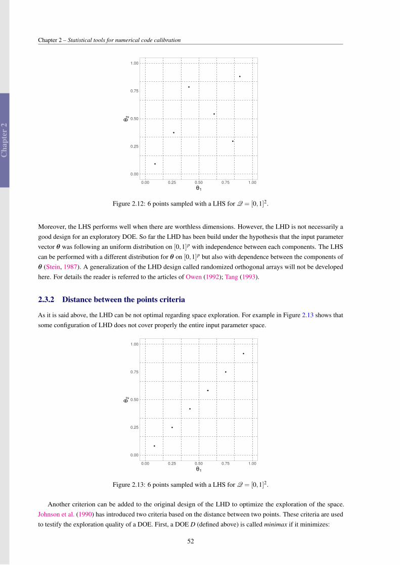
Cha

pter

2

Chapter 2 – Statistical tools for numerical code calibration

0.00

0.25

0.50

0.75

1.00

0.00 0.25 0.50 0.75 1.00θ1

θ2

Figure 2.12: 6 points sampled with a LHS for Q = [0,1]2.

Moreover, the LHS performs well when there are worthless dimensions. However, the LHD is not necessarily agood design for an exploratory DOE. So far the LHD has been build under the hypothesis that the input parametervector θ was following an uniform distribution on [0,1]p with independence between each components. The LHScan be performed with a different distribution for θ on [0,1]p but also with dependence between the components ofθ (Stein, 1987). A generalization of the LHD design called randomized orthogonal arrays will not be developedhere. For details the reader is referred to the articles of Owen (1992); Tang (1993).

2.3.2 Distance between the points criteria

As it is said above, the LHD can be not optimal regarding space exploration. For example in Figure 2.13 shows thatsome configuration of LHD does not cover properly the entire input parameter space.

0.00

0.25

0.50

0.75

1.00

0.00 0.25 0.50 0.75 1.00θ1

θ2

Figure 2.13: 6 points sampled with a LHS for Q = [0,1]2.

Another criterion can be added to the original design of the LHD to optimize the exploration of the space.Johnson et al. (1990) has introduced two criteria based on the distance between two points. These criteria are usedto testify the exploration quality of a DOE. First, a DOE D (defined above) is called minimax if it minimizes:

52

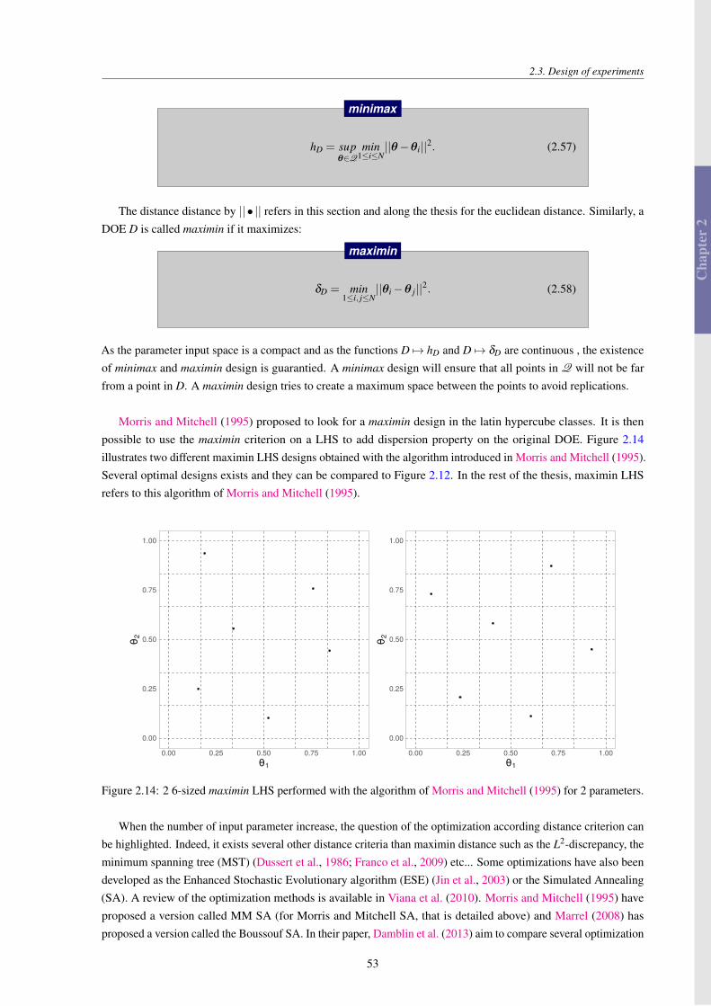
Cha

pter

2

2.3. Design of experiments

hD = supθ∈Q

min1≤i≤N

||θ−θi||2. (2.57)

minimax

The distance distance by || • || refers in this section and along the thesis for the euclidean distance. Similarly, aDOE D is called maximin if it maximizes:

δD = min1≤i, j≤N

||θi−θ j||2. (2.58)

maximin

As the parameter input space is a compact and as the functions D 7→ hD and D 7→ δD are continuous , the existenceof minimax and maximin design is guarantied. A minimax design will ensure that all points in Q will not be farfrom a point in D. A maximin design tries to create a maximum space between the points to avoid replications.

Morris and Mitchell (1995) proposed to look for a maximin design in the latin hypercube classes. It is thenpossible to use the maximin criterion on a LHS to add dispersion property on the original DOE. Figure 2.14illustrates two different maximin LHS designs obtained with the algorithm introduced in Morris and Mitchell (1995).Several optimal designs exists and they can be compared to Figure 2.12. In the rest of the thesis, maximin LHSrefers to this algorithm of Morris and Mitchell (1995).

0.00

0.25

0.50

0.75

1.00

0.00 0.25 0.50 0.75 1.00θ1

θ2

0.00

0.25

0.50

0.75

1.00

0.00 0.25 0.50 0.75 1.00θ1

θ2

Figure 2.14: 2 6-sized maximin LHS performed with the algorithm of Morris and Mitchell (1995) for 2 parameters.

When the number of input parameter increase, the question of the optimization according distance criterion canbe highlighted. Indeed, it exists several other distance criteria than maximin distance such as the L2-discrepancy, theminimum spanning tree (MST) (Dussert et al., 1986; Franco et al., 2009) etc... Some optimizations have also beendeveloped as the Enhanced Stochastic Evolutionary algorithm (ESE) (Jin et al., 2003) or the Simulated Annealing(SA). A review of the optimization methods is available in Viana et al. (2010). Morris and Mitchell (1995) haveproposed a version called MM SA (for Morris and Mitchell SA, that is detailed above) and Marrel (2008) hasproposed a version called the Boussouf SA. In their paper, Damblin et al. (2013) aim to compare several optimization

53

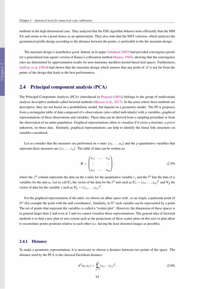
Cha

pter

2

Chapter 2 – Statistical tools for numerical code calibration

methods in the high dimensional case. They analyzed that the ESE algorithm behaves more efficiently than the MMSA and seems to be a good choice as an optimization. They also state that the MST criterion, which analyzes thegeometrical profile design according to the distance between the points, is preferable to the the maximin design.

The maximin design is nonetheless good. Indeed, in its paper Schaback (2007) had provided convergence proofsfor a generalized non-square version of Kansa’s collocation method (Kansa, 1985), showing that the convergencerates are determined by approximation results for non-stationary meshless-kernel-based trial spaces. Furthermore,Auffray et al. (2010) had shown that the maximin design which ensures that any point of Q is not far from thepoints of the design that leads to the best performances.

2.4 Principal component analysis (PCA)

The Principal Component Analysis (PCA) (introduced in Pearson (1901)) belongs to the group of multivariateanalysis descriptive methods called factorial methods (Husson et al., 2017). In the sense where these methods aredescriptive, they are not based on a probabilistic model, but depend on a geometric model. The PCA proposes,from a rectangular table of data composed of n observations (also called individuals) with p variables, graphicalrepresentations of these observations and variables. These data can be derived from a sampling procedure or fromthe observation of an entire population. Graphical representations allow to visualize if it exists a structure, a priori

unknown, on these data. Similarly, graphical representations can help to identify the linear link structures onvariables considered.

Let us consider that the measures are performed on n units u1, . . . ,un and the p quantitative variables thatrepresent these measures are v1, . . . ,vp. The table of data can be written as:

X =

x11 . . . x1p...

...xn1 . . . xnp

, (2.59)

where the jth column represents the data on the n units for the quantitative variable v j and the ith line the data of p

variables for the unit ui. Let us call Ui the vector of the data for the ith unit such as Ui = (xi1, . . . ,xip)T and Vj the

vector of data for the variable j such as Vj = (x1 j, . . . ,xn j)T .

For the graphical representation of the units, we choose an affine space with , as an origin, a particular point ofRp (for example the point with the null coordinates). Similarly, in Rn each variable can be represented by a point.The set of points that represent the variables is called a “scatter plot”. However, the dimension of these spaces isin general larger than 2 and even at 3 and we cannot visualize these representations. The general idea of factorialmethods is to find a new plan or axis system such as the projections of these scatter plots on this axis or plan allowto reconstitute points positions relative to each other (i.e. having the least distorted images as possible).

2.4.1 Distance

To make a geometric representation, it is necessary to choose a distance between two points of the space. Thedistance used by the PCA is the classical Euclidean distance:

d2(ui,ui′) =p

∑j=1

(xi j− xi′ j)2. (2.60)

54

Cha

pter

2

2.4. Principal component analysis (PCA)

With this distance, all the variables are playing the same role and the axes defined by the variables are constitutingan orthogonal basis. A dot product can be associated to this distance:

〈 →oui,→

oui′〉=p

∑j=1

xi jxi′ j =UTi Ui′ , (2.61)

as well as a norm:

|| →oui||2 =p

∑j=1

x2i j =U

Ti Ui. (2.62)

We can then define the angle α between two vectors by its cosine:

cos(α) =〈 →oui,

→oui′〉

|| →oui|| ||→

oui′ ||=

UTi Ui′√

(UTi Ui)(U

Ti′ Ui′)

. (2.63)

The point with null coordinates is not always a satisfactory origin because if the coordinates of the points in thescatter plot are high, the plotted points are far away from the origin. It seems wiser to chose an origin linked to thescatter plot itself: the center of gravity. We will consider for the following that we center the matrixX such as:

Xc =

x11− x•1 . . . x1p− x•p

......

xn1− x•1 . . . xnp− x•p

. (2.64)

where x•p is the mean of the corresponding column inX . The coordinates of the vectors Ui and Vj are alsocentered and can be written as:

Uci =

xi1− x•1

...xip− x•p

,and Vc j =

xi j− x• j

...xn j− x• j

. (2.65)

2.4.2 Moments of inertia

Les us note IG the moment of inertia of the individuals scatter plot with respect to the center of gravity G:

IG =1n

n

∑i=1

d2(G,ui) =1n

n

∑i=1

p

∑j=1

(xi j− x• j)2 =

1n

n

∑i=1UT

ciUci. (2.66)

This moment of total inertia is of interest because it measures the dispersion of the individual scatter plot fromthe center of gravity. If this moment of inertia is large, it means the scatter plot is dispersed. However, if it is small,the scatter plot is highly concentrated on its center of gravity. Another way to write Equation (2.66) can be obtainedby inverting the sums:

IG =p

∑j=1

[1n

n

∑i=1

(xi j− x• j)2]=

p

∑j=1

Var(v j), (2.67)

where Var(v j) is the empirical variance of the variable v j. From this form, it can be seen that total inertia isequal to the trace of the covariance matrix Σ of the p variables v j:

IG = trace(Σ). (2.68)

55

Cha

pter

2

Chapter 2 – Statistical tools for numerical code calibration

The inertia of the scatter plot from an axis ∆ passing by G is by definition:

I∆ =1n

n

∑i=1

d2(h∆i,ui), (2.69)

where h∆i is the orthogonal projection of ui on ∆. This inertia measures the proximity of the scatter plot to the axis∆.

The inertia of the scatter plot from a linear subspace V passing by G, is similarly defined, and is equal to:

IV =1n

n

∑i=1

d2(hVi,ui), (2.70)

where hVi is the orthogonal projection of ui on the linear subspace V . Let us not V ∗ the orthogonal complementof V in Rp and hV ∗i the orthogonal projection of ui on V ∗. By the Pythagorean theorem:

d2(hVi,ui)+d2(hV ∗i,ui) = d2(G,ui) = d2(G,hVi)+d2(G,hV ∗i). (2.71)

From Equation (2.71), it can be concluded that:

IV + IV ∗ = IG. (2.72)

Huygens theorem

In the particular case where the linear subspace V has a dimension of 1, IV ∗ is a measure of the scatter plotelongation along the axis of the linear subspace. By projecting the scatter plot on a linear subspace V , the inertiameasured by IV is lost (only IV ∗ is kept). If Rp is decomposed in a sum of orthogonal linear subspace such as:

∆1⊕∆2⊕·· ·⊕∆p, (2.73)

then (with a Pythagorean theorem):IG = I∆∗1

+ · · ·+ I∆∗p . (2.74)

2.4.3 Axis of minimum inertia

The axis ∆1 which is the closest to all the individuals in the scatter plot is an axis passing by G and has the minimuminertia I∆1 . This axis is interesting because, when the projection will be done, this will give the least distorted imageof the scatter plot. Looking for ∆1 such as I∆1 is minimum is equivalent to look for ∆1 such as I∆∗1

is maximum

(Equation (2.74)). Let us note the unitary vector→

Ga1 of the axis ∆1. Then, the vector→

Ga1 is looked for such as I∆∗1

is maximum under the constraint of ||→

Ga1||2 = 1.

We can write:d2(G,h∆1i) = 〈

→Gui,

→Ga1〉2 = aT

1UciUTci a1. (2.75)

Using the property of symmetry of the dot product, it can be deduced that:

I∆∗1=

1n

n

∑i=1

aT1UciU

Tci a1 = aT

1

[1n

n

∑i=1UciU

Tci

]a1. (2.76)

56

Cha

pter

2

2.4. Principal component analysis (PCA)

The empirical variance Σ of the p variables is identified under the bracket of Equation (2.76). Then:

I∆∗1= aT

1 Σa1, (2.77)

with,

||→

Ga1||2 = aT1 a1. (2.78)

The problem is summarized at finding a1 that maximize aT1 Σa1 under the constraint aT

1 a1 = 1. The componentsof a1 are unknown and are linked by a constraint. To solve such a problem, a Lagrange multiplier method canbe used. This method consists in finding the optimums of a function f (t1, . . . , tp) where the p variables arelinked by a relation l(t1, . . . , tp) = cte. The p partial derivatives with respect to each variable of the functiong(t1, . . . , tp) = f (t1, . . . , tp)−λ (l(t1, . . . , tp)− cte) are calculated and annulled to get a system of p+1 equationswith p+1 variables (after adding the constraint term). The term λ is called the Lagrange multiplier. In the previouscase, partial derivatives of

g(a1) = g(a11, . . . ,a1p) = aT1 Σa1−λ1(aT

1 a1−1) (2.79)

has to be found. Using the derivative of a quadratic form with respect of a vector, it can be proven that:

∂g(a1)

∂a1= 2Σa1−2λ1a1 = 0. (2.80)

The system to solver is then: Σ−λ1a1 = 0 (1)

aT1 a1−1 = 0 (2)

(2.81)

From Equation (2.81), matrix Equation (1) allows to show that a1 is an eigenvector of Σ with eigenvalue λ1.Multiplying matrix Equation (1) by aT

1 on the left

aT1 Σa1−λ1aT

1 a1 = 0 (2.82)

is obtained and using the Equation (2) in Equation 2.81, it is shown that:

aT1 Σa1 = λ1. (2.83)

From Equation (2.77), the first term of Equation (2.83) is replaced and it can be stated that λ1 = I∆∗1. That means

the value λ1 is the highest eigenvalue of Σ and this eigenvalue is the inertia carried by ∆1. Then, the axis ∆1 has forunit vector the first eigenvector associated at the highest eigenvalue of the covariance matrix Σ.

However, only one axis might not be sufficient to represent all the data. Then, a second axis ∆2 is looked forwhich is orthogonal to ∆1 and has a minimal inertia. Identically as before, let us define the axis ∆2 passing by G anddefined by its unit vector u2. The inertia of the individuals scatter plot with respect to it orthogonal complement is:

I∆∗2= aT

2 Σa2. (2.84)

The inertia defined Equation (2.84) has to be maximum under the constraints:

aT2 a2 = 1 and aT

2 a1 = 0. (2.85)

57

Cha

pter

2

Chapter 2 – Statistical tools for numerical code calibration

The second constraint Equation (2.85) represents the orthogonality of u1 with u2. With the Lagrange multipliersmethod, but with two constraints, it can be shown that a2 is the eigenvector of the covariance matrix Σ whichcorresponds to the second highest eigenvalue. It can be also demonstrated that the inertia is maximum in the linearsubspace defined with the unit vectors u1 and u2.

The same procedure can be extended but can only be done p times. The covariance matrix Σ is real andsymmetrical, thus it has only p eigenvectors (building an orthogonal basis of Rp).

2.4.4 Contribution to the total inertia

All the axes does not have the same contribution on the total inertia. Using the Huygens theorem Equation 2.72, thetotal inertia can be decomposed as:

IG = I∆∗1+ · · ·+ I∆∗p = λ1 + · · ·+λp. (2.86)

The absolute contribution to the total inertia of the axis ∆k is equal to:

ca(∆k/IG) = λk, (2.87)

but its relative contribution is defined as:

cr(∆k/IG) =λk

IG. (2.88)

For the rest of the thesis, the term “percent of inertia explained by the axis ∆k” will be used as a reference of therelative contribution. It is possible to extend these definitions at all the generated linear subspaces. For example, thepercent of inertia explained by the linear subspace generated by the two eigenvector associated at the two highesteigenvalues is defined as:

cr(∆1⊕∆2/IG) =λ1 +λ2

IG. (2.89)

These inertia percentages are indicators of the part of variability of the scatter plot explained by these subspaces.Practically, only the d (d < p) first axis are considered because they explain a percentage of inertia close to 1. Theother axes are then neglected.

2.4.5 Graphical representations

Individuals representation quality

To have a graphical representation of the individuals in the plans defined by the new axis, it is necessary to calculatethe coordinates of each individuals in the new axis. To get yik the coordinate of the unit ui on the axis ∆ j, an

orthogonal projection of the vector→

Gui is achieved:

yik = 〈→

Gui,→ak〉= aT

kUci, (2.90)

and,Yi =A

TUci, (2.91)

where Yi is the vector of coordinates of the unit ui andA is the change of basis matrix (A is the matrix composedof the orthogonal eigenvectors, which have a norm equal to 1, is an orthogonal matrix and its inverse is equal to its

58

Cha

pter

2

2.4. Principal component analysis (PCA)

transposed).

The square of the cosine of the angle αik between→

Gui and an axis ∆k is equal to:

cos2(αik) =〈→

Gui,→

Gak〉2

||→

Gui||2=

aTkUciU

Tci ak

UTciUci

=

[∑

pj=1(xi j− x• j)ak j

]2

∑pj=1(xi j− x• j)2 . (2.92)

As mentioned above, by using the Pythagorean theorem, the square of the cosine of the angle αikk′ between→

Gui

and the plan generated by the two axes ∆k⊕∆k′ can be calculated and:

cos2(αikk′) = cos2(αik)+ cos2(αik′). (2.93)

Contribution of an individual to an axis

When I∆∗k(the inertia carried by the axes ∆k) is calculated, it is possible to see the part of the inertia attributable to

an individual ui in particular. From Equation (2.70), I∆∗k= 1

n ∑ni=1 d2(h∆ki ,G) and the absolute contribution of ui of

this inertia is:ca(ui/∆k) =

1n

d2(h∆ki ,G), (2.94)

because all the individuals have the same weight. Practically, an individual will have a greater contribution to theaxis when its projection will be far from the center of gravity. The other way around, an individual which has aprojection close to the center of gravity will have a weak contribution to the axis. It is also possible, for the sameparticular individual ui, to give its relative contribution to the inertia carried by ∆k:

cr(ui/∆k) =1n d2(h∆ki ,G)

I∆∗k

=1n 〈→

Gui,→

Gak〉2

λk=

1n aT

kUciUTci ak

λk. (2.95)

Note that ∑ni=1 cr(ui/∆k) = 1.

Graphical representation of the variables

The individuals have been represented in the space of the original variables and the change of basis has been madein this original space. New axes are then linear combination of original axes and can be considered as new variableswhich are a linear combination of original variables. These new variables are called “principal components”. Let usnote Z1, . . . ,Zp the principal components, Zk being the new variable corresponding to the axes ∆k and:

Zk =p

∑j=1

ak jVc j =Xcak, (2.96)

where Vc j is the centered variable vector defined in Equation (2.65) and Xc the matrix of centering dataintroduced Equation (2.64). In general, the principal components can be written as:

Z = [Z1, . . . ,Zp] =XcA. (2.97)

It is also interesting to visualize how original variables are linked to the principal components by calculating thecorrelations. Original variables representation will be done by taking as coordinates the correlation coefficients withthe new variables. This representation is called “correlation circle” because of the fact that a correlation coefficientis always between −1 and 1 which leads to have all the points in a circle of radius 1. The variances of the principalcomponents are:

59

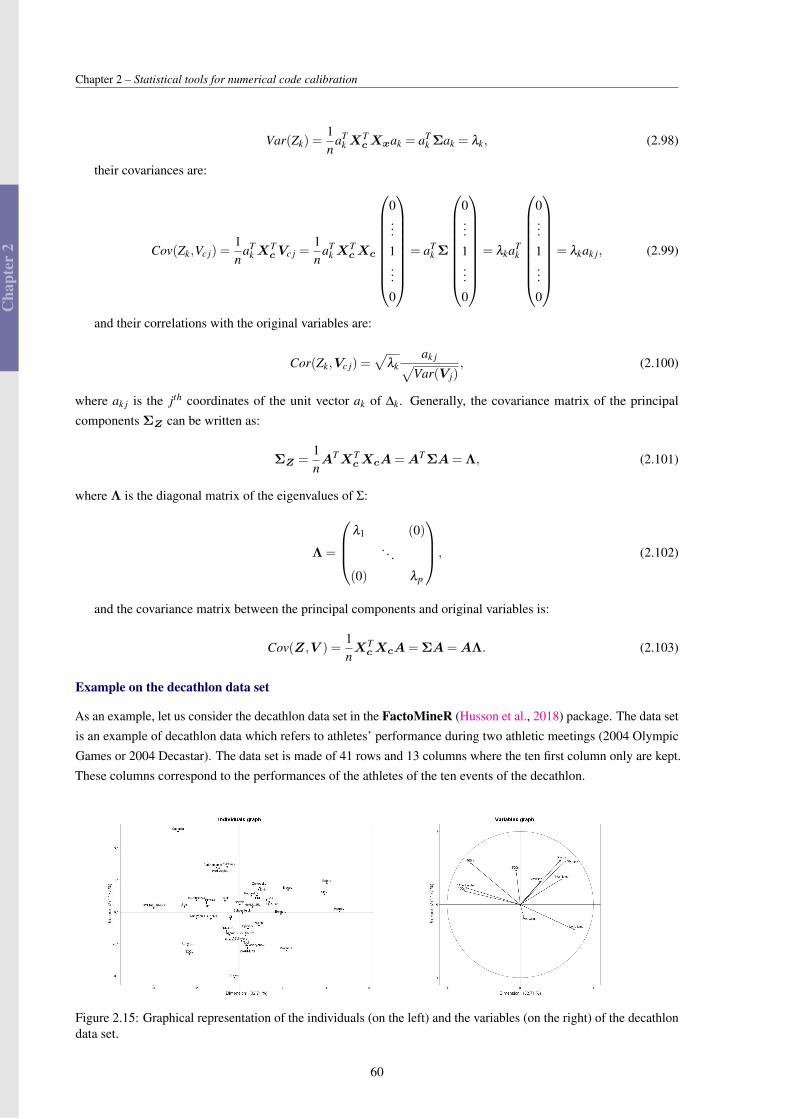
Cha

pter

2

Chapter 2 – Statistical tools for numerical code calibration

Var(Zk) =1n

aTkX

TcXxak = aT

k Σak = λk, (2.98)

their covariances are:

Cov(Zk,Vc j) =1n

aTkX

TcVc j =

1n

aTkX

TcXc

0...1...0

= aT

k Σ

0...1...0

= λkaT

k

0...1...0

= λkak j, (2.99)

and their correlations with the original variables are:

Cor(Zk,Vc j) =√

λkak j√

Var(V j), (2.100)

where ak j is the jth coordinates of the unit vector ak of ∆k. Generally, the covariance matrix of the principalcomponents ΣZ can be written as:

ΣZ =1nATXT

cXcA=AT ΣA= Λ, (2.101)

where Λ is the diagonal matrix of the eigenvalues of Σ:

Λ =

λ1 (0)

. . .

(0) λp

, (2.102)

and the covariance matrix between the principal components and original variables is:

Cov(Z,V ) =1nXTcXcA= ΣA=AΛ. (2.103)

Example on the decathlon data set

As an example, let us consider the decathlon data set in the FactoMineR (Husson et al., 2018) package. The data setis an example of decathlon data which refers to athletes’ performance during two athletic meetings (2004 OlympicGames or 2004 Decastar). The data set is made of 41 rows and 13 columns where the ten first column only are kept.These columns correspond to the performances of the athletes of the ten events of the decathlon.

Figure 2.15: Graphical representation of the individuals (on the left) and the variables (on the right) of the decathlondata set.

60

Cha

pter

2

2.5. Monte Carlo Markov Chains techniques

Figure 2.15 represents the individuals and the variables of the decathlon data set. For each axis, the percentageof the inertia carried is indicated and both axis (the ones used for the representation) contain 50% of the totalinertia. The right panel of Figure 2.15 illustrates the correlation between the variables and for example the variable“100m” is negatively correlated with the variable “long.jump”. This means that when an athlete jumps far, hedoes not achieve so good performances in the 100m. The left panel of Figure 2.15 illustrates in two axis a globalrepresentation of the performances of the athletes. The first axis strongly represents the speed events and long jumpevent (given from the right panel of Figure 2.15). This means for an individual that has a high value on this axis, heis more likely better on these events than an individual that has a weak value on the axis. For example Karpov seemsto have better performed than Bourguignon in these events. The second axis represents the variables “Discuss” and“shot put” and similarly a high value of the individual on this axis means that he performed well on these events.The winner of the 2004 Olympic Games is Sebrie who has reasonable value on both axis. The variable “Discus”,“Shot.put” and “High.jump” are not correlated to “100m”, “400m”, “110m.hurdle” and “Long.jump” which meansthat strength and speed are not correlated.

2.5 Monte Carlo Markov Chains techniques

Sampling from a posterior distribution is the only mean to get information about the posterior distribution if thereis no conjugacy in the model. Several Monte Carlo Markov Chains (MCMC) have been developed in that sense(Robert and Casella, 2013; Andrieu et al., 2003). Let us consider a general example, in a Bayesian framework,where the posterior density of a p dimensional parameter vector θ is looked for. Let us define a probability space(Ω,F ,π) where Ω stands for a sample space, F a σ -algebra on Ω and π a probability on F . The parameter vectoris defined as θ ∈Q ⊂ Rp and the n dimensional experimental vector as y ∈ E ⊂ Rn. From Bayes formula, it ispossible to write straightforwardly that:

π(θ|y) = L (y;θ)π(θ)m(y)

, (2.104)

where m(y) =∫θ∈Q L (y;θ)π(θ), but as the term m(y) is independent from θ, Equation (2.104) can be

rewritten as:π(θ|y) ∝ L (y;θ)π(θ). (2.105)

When the prior distribution is not conjugate to the the likelihood, π(θ|y) cannot be expressed analytically. Thechoice of the sampling method is partly conditioned by the knowledge of full conditional distributions (i.e. theknowledge of π(θi|y,θ(−i)) ∀i ∈ [1, . . . ,n], θ(−i) representing the vector θ without the ith component). In casewhere these full conditional distributions are known, the Gibbs sampler can be used. Otherwise, Metropolis Hastingsalgorithms could be applied to sample in the posterior distribution. The full conditional distribution can be writtenproportionally to the joint distribution such as:

π(θi|y,θ−i) =π(θ,y)

π(θ1, . . . ,θi−1,θi+1, . . . ,θp,y)∝ π(θ,y). (2.106)

Then from Equation (2.105):

π(θi|θ−i,y) ∝ L (y;θ)π(θ)

∝ L (y;θ)π(θ1|θ2, . . . ,θp)π(θ2|θ3, . . . ,θp) . . .π(θp−1|θp)π(θp).(2.107)

61

Cha

pter

2

Chapter 2 – Statistical tools for numerical code calibration

And, if all the components of θ are independent then:

π(θi|θi,y) ∝ L (y;θ)p

∏i=1

π(θi). (2.108)

The aim of the MCMC is then to produce a Markov chain whose invariant distributionis the posterior distribution

MCMC goal

2.5.1 Gibbs sampler

If the full conditional distributions are known, then it is possible to sample in each of them. This way, if an initialstate θ(s), such as θ(s) = (θ

(s)1 , . . . ,θ

(s)p ), is considered, a new state can be sampled from:

1. sample θ(s+1)1 ∼ π(θ

(s)1 |θ

(s)2 , . . . ,θ

(s)p ,y)

2. sample θ(s+1)2 ∼ π(θ

(s)2 |θ

(s)1 ,θ

(s)3 , . . . ,θ

(s)p ,y)

...

(p). sample θ(s+1)p ∼ π(θ

(s)p |θ(s)1 , . . . ,θ

(s)p−1,y)

(p+1). θ(s+1) = (θ(s+1)1 , . . . ,θ

(s+1)p )

The algorithm that repeats this sequence S times is called Gibbs sampler and generates a dependent sequence ofparameters: θ = θ(1), . . . ,θ(S) (Robert and Casella, 2013; Hoff, 2009). The algorithm can be written as:

Algorithm 1 Gibbs sampler

θ(1) = θinitfor i in 2 : S do

for j in 1 : p doθ(i)j ∼ π(θ

(i−1)j |θ(i)1... j−1,θ

(i)j+1...p,y)

end forθ(i) = (θ

(i)1 , . . . ,θ

(i)p )

end for

For example, let us consider a sample of data y such as each component are a realization of the random variableY which is following Y ∼N (µ, 1

τ) where µ is the population mean and τ the population precision (inverse of the

variance). Let us consider n the sample size, y the sample mean and s2 the sample variance. A priori, there is nocorrelation between the population mean and the population variance:

π(µ,τ) = π(µ)π(τ). (2.109)

Considering that π(µ) ∝ 1 and π(τ) ∝ τ−1 as prior densities (Casella and George, 1992), the conditionalposterior densities are explicit and can be expressed as:

62

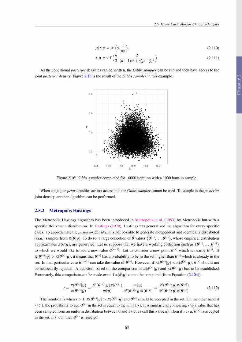
Cha

pter

2

2.5. Monte Carlo Markov Chains techniques

µ|τ,y∼N(

y,1

nτ

), (2.110)

τ|µ,y∼ Γ

(n2,

2(n−1)s2 +n(µ− y)2

). (2.111)

As the conditional posterior densities can be written, the Gibbs sampler can be run and then have access to thejoint posterior density. Figure 2.16 is the result of the Gibbs sampler in this example.

0.2

0.4

0.6

0.8

13.5 14.0 14.5 15.0 15.5 16.0μ

τ

Figure 2.16: Gibbs sampler completed for 10000 iteration with a 1000 burn-in sample.

When conjugate prior densities are not accessible, the Gibbs sampler cannot be used. To sample in the posterior

joint density, another algorithm can be performed.

2.5.2 Metropolis Hastings

The Metropolis Hastings algorithm has been introduced in Metropolis et al. (1953) by Metropolis but with aspecific Boltzmann distribution. In Hastings (1970), Hastings has generalized the algorithm for every specificcases. To approximate the posterior density, it is not possible to generate independent and identically distributed(i.i.d.) samples from π(θ|y). To do so, a large collection of θ values θ(1), . . . ,θ(s), whose empirical distributionapproximates π(θ|y), are generated. Let us suppose that we have a working collection such as θ(1), . . . ,θ(s)to which we would like to add a new value θ(s+1). Let us consider a new point θ(∗) which is nearby θ(s). Ifπ(θ(∗)|y)> π(θ(s)|y), it means that θ(∗) has a probability to be in the set higher than θ(s) which is already in theset. In that particular case θ(s+1) can take the value of θ(∗). However, if π(θ(∗)|y) < π(θ(s)|y), θ (∗) should notbe necessarily rejected. A decision, based on the comparison of π(θ(∗)|y) and π(θ(s)|y) has to be established.Fortunately, this comparison can be made even if π(θ|y) cannot be computed (from Equation (2.104)):

r =π(θ(∗)|y)π(θ(s)|y)

=L (θ(∗);y)π(θ(∗))

m(y)

m(y)

L (θ(s);y)π(θ(s))=

L (θ(∗);y)π(θ(∗))L (θ(s);y)π(θ(s))

. (2.112)

The intuition is when r > 1, π(θ(∗)|y)> π(θ(s)|y) and θ(∗) should be accepted in the set. On the other hand ifr < 1, the probability to add θ(∗) in the set is equal to the min(1,r). It is similarly as comparing r to a value that hasbeen sampled from an uniform distribution between 0 and 1 (let us call this value u). Then if r > u, θ(∗) is acceptedin the set, if r < u, then θ(∗) is rejected.

63

Cha

pter

2

Chapter 2 – Statistical tools for numerical code calibration

The new point θ(∗), which is nearby θ(s), is generated from a proposal distribution (also called jumping

distribution in Gelman et al. (1995)). This distribution q(θ(∗)|θ(s)) can be distinguished in two cases. The first, thedistribution is symmetric such as q(θ(∗)|θ(s)) = q(θ(s)|θ(∗)) which is the case for:

• q(θ(∗)|θ(s)) = uniform(θ(s)−δ ,θ(s)+δ ),

• q(θ(∗)|θ(s)) = normal(θ(s),kΣ2).

In that particular case the algorithm is called Metropolis algorithm and the computation of the ratio is straight-forwardly obtained from Equation (2.112). Algorithm 2 recalls the steps of this particular MCMC.

Algorithm 2 Metropolis algorithm

θ(1) = θinitτaccept = 0for i in 1 : S doθ(∗) ∼N (θ(i),kΣ)

r = π(θ(∗)|y)π(θ(i)|y)

= π(θ(∗))L (θ(∗);y)π(θ(i))L (θ(i);y)

if r > u, with u∼U (0,1) thenθ(i+1) = θ(∗)

τaccept = τaccept +1elseθ(i+1) = θ(i)

end ifend forθM = θ[Nburn−in : S]

On the other hand if q(θ(∗)|θ(s)) is not symmetric, the ratio is now given by:

r =L (θ(∗);y)π(θ(∗))L (θ(s);y)π(θ(s))

q(θ(s)|θ(∗))q(θ(∗)|θ(s))

. (2.113)

The ratio is almost surely defined because a jump can only occur if both q(θ(∗)|θ(s)) and q(θ(s)|θ(∗)) are nonzero. Such a proposal can be useful for increasing the speed of the random walk. Algorithm 3 details the steps ofthe, so-called, Metropolis Hastings algorithm.

Algorithm 3 Metropolis Hastings algorithm

θ(1) = θinitτaccept = 0for i in 1 : S doθ(∗) ∼ q(θ(i), .)

r = π(θ(∗)|y)q(θ(∗),θ(i))π(θ(i)|y)q(θ(i),θ(∗)) =

π(θ(∗))L (θ(∗);y)q(θ(∗),θ(i))π(θ(i))L (θ(i);y)q(θ(i),θ(∗))

if r > u, with u∼U (0,1) thenθ(i+1) = θ(∗)

τaccept = τaccept +1elseθ(i+1) = θ(i)

end ifend forθMH = θ[Nburn−in : S]

The choice of the nature of q is problem relevant. To simplify the programing, it is common to choose aMetropolis algorithm. It is difficult to tune all the parameters of a Metropolis algorithm, so it simplifies this problem

64

Cha

pter

2

2.5. Monte Carlo Markov Chains techniques

if a symmetric proposal distribution is taken. Between the normal or the uniform random walk, the major difficultyis to tune the parameter k or δ . The performance of such an algorithm is evaluated by its faculty to explore the inputparameter space Q. So, if Q ⊂ Rp with p high, then it is hard to find the right convergence direction.

In the case where the Metropolis is chosen with a normal proposal distribution, some improvements can bebrought especially when p is high.

2.5.3 Metropolis within Gibbs

When the number of parameter of parameter is high, the input parameter space becomes a space where it iscomplicated to move in the right direction. If the access of conditional distributions are available, one solution couldbe to compute the ratio according to the conditional distribution relative to the active parameter. Then, the algorithmwould move parameter by parameter, that increases the efficiency of the displacement. The ratio introduced inEquation (2.112) becomes:

r =π(θ

(∗)j |θ

(∗)− j ,y)

π(θ(s)j |θ

(s)− j,y)

=π(θ

(∗)j )L (θ

(∗)j ;θ(∗)1... j−1,θ

(∗)j+1...p,y)

π(θ(S)j )L (θ

(s)j ;θ(s)1... j−1,θ

(s)j+1...p,y)

. (2.114)

Algorithm 4 Metropolis within Gibbs algorithm

θ(1) = θinitτaccept = (0, . . . ,0)T

for i in 1 : S dofor j in 1 : p doθ(∗)j ∼N (θ

(i)j ,kΣ[ j, j])

r =π(θ

(∗)j )L (θ

(∗)j ;θ(∗)1... j−1,θ

(∗)j+1...p,y)

π(θ(i)j )L (θ

(i)j ;θ(i)1... j−1,θ

(i)j+1...p,y)

if r > u, with u∼U (0,1) thenθ(i+1)j = θ

(∗)

τaccept j = τaccept j +1else

θ(i+1)j = θ

(i)j

end ifend for

end forθMWG = θ[Nburn−in : S]

The strength of Algorithm 4 is to sample well in a multidimensional space. However, as it is moving componentby component, it is more time consuming than a regular Metropolis or Metropolis Hastings algorithm.

2.5.4 Improvements of the Metropolis Hastings

The major difficulty in applying a Metropolis Hastings algorithm is to use a right proposal distribution such as thenew point point is neither too far from the previous one or too close. The acceptation ratio controls the quality ofthe chain. If the acceptation ratio is too high, it means that the number of the new accepted points is too high andthat the proposal distribution is not adequate to the problem because it generates points too close to the previousone. Similarly, a too low acceptation ratio is synonym of a proposal distribution that generates points that are toofar from the previous one. Let us consider for the rest of this section (and for the major part of the thesis) that theconsidered proposal distribution is normal centered on the previous point and with variance covariance kΣ. Theproposal distribution is in that case symmetric and the major difficulty is to find the right k and Σ that make a good

65

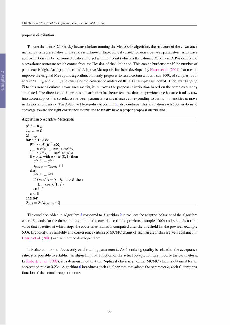
Cha

pter

2

Chapter 2 – Statistical tools for numerical code calibration

proposal distribution.

To tune the matrix Σ is tricky because before running the Metropolis algorithm, the structure of the covariancematrix that is representative of the space is unknown. Especially, if correlation exists between parameters. A Laplaceapproximation can be performed upstream to get an initial point (which is the estimate Maximum A Posteriori) anda covariance structure which comes from the Hessian of the likelihood. This can be burdensome if the number ofparameter is high. An algorithm, called Adaptive Metropolis, has been developed by Haario et al. (2001) that tries toimprove the original Metropolis algorithm. It mainly proposes to run a certain amount, say 1000, of samples, withat first Σ = Ip and k = 1, and evaluates the covariance matrix on the 1000 samples generated. Then, by changingΣ to this new calculated covariance matrix, it improves the proposal distribution based on the samples alreadysimulated. The direction of the proposal distribution has better features than the previous one because it takes nowinto account, possible, correlation between parameters and variances corresponding to the right intensities to movein the posterior density. The Adaptive Metropolis (Algorithm 5) also continues this adaptation each 500 iterations toconverge toward the right covariance matrix and to finally have a proper proposal distribution.

Algorithm 5 Adaptive Metropolis

θ (1) = θinitτaccept = 0Σ = Ipfor i in 1 : S do

θ (∗) ∼N (θ (i),kΣ)

r = π(θ (∗)|y)π(θ (i)|y)

= π(θ (∗))L (θ (∗);y)π(θ (i))L (Θi;y)

if r > u, with u∼U (0,1) thenθ (i+1) = θ (∗)

τaccept = τaccept +1else

θ (i+1) = θ (i)

if i mod A = 0 & i > B thenΣ = cov(θ [1 : i])

end ifend if

end forΘAM = Θ[Nburn−in : S]

The condition added in Algorithm 5 compared to Algorithm 2 introduces the adaptive behavior of the algorithmwhere B stands for the threshold to compute the covariance (in the previous example 1000) and A stands for thevalue that specifies at which steps the covariance matrix is computed after the threshold (in the previous example500). Ergodicity, reversibility and convergence criteria of MCMC chains of such an algorithm are well explained inHaario et al. (2001) and will not be developed here.

It is also common to focus only on the tuning parameter k. As the mixing quality is related to the acceptanceratio, it is possible to establish an algorithm that, function of the actual acceptation rate, modify the parameter k.In Roberts et al. (1997), it is demonstrated that the “optimal efficiency” of the MCMC chain is obtained for anacceptation rate at 0.234. Algorithm 6 introduces such an algorithm that adapts the parameter k, each C iterations,function of the actual acceptation rate.

66

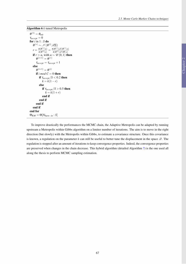
Cha

pter

2

2.5. Monte Carlo Markov Chains techniques

Algorithm 6 k tuned Metropolis

θ (1) = θinitτaccept = 0for i in 1 : S do

θ (∗) ∼N (θ (i),kΣ)

r = π(θ (∗)|y)π(θ (i)|y)

= π(θ (∗))L (θ (∗);y)π(θ (i))L (Θi;y)

if r > u, with u∼U (0,1) thenθ (i+1) = θ (∗)

τaccept = τaccept +1else

θ (i+1) = θ (i)

if i mod C = 0 thenif τaccept/S < 0.2 then

k = k(1− r)else

if τaccept/S > 0.5 thenk = k(1+ r)

end ifend if

end ifend if

end forΘKM = Θ[Nburn−in : S]

To improve drastically the performances the MCMC chain, the Adaptive Metropolis can be adapted by runningupstream a Metropolis within Gibbs algorithm on a limiter number of iterations. The aim is to move in the rightdirection (but slowly) with the Metropolis within Gibbs, to estimate a covariance structure. Once this covarianceis known, a regulation on the parameter k can still be useful to better tune the displacement in the space Q. Theregulation is stopped after an amount of iterations to keep convergence properties. Indeed, the convergence propertiesare preserved when changes in the chain decrease. This hybrid algorithm (detailed Algorithm 7) is the one used allalong the thesis to perform MCMC sampling estimation.

67

Cha

pter

2

Chapter 2 – Statistical tools for numerical code calibration

Algorithm 7 Hybrid Metropolis

θ(1) = θinitτaccept = (0, . . . ,0)T

for i in 1 : SMWG dofor j in 1 : p doθ(∗)j ∼N (θ

(i)j ,kΣ[ j, j])

r =π(θ

(∗)j )L (θ

(∗)j ;θ(∗)1... j−1,θ

(∗)j+1...p,y)

π(θ(i)j )L (θ

(i)j ;θ(i)1... j−1,θ

(i)j+1...p,y)

if r > u, with u∼U (0,1) thenθ(i+1)j = θ

(∗)

τaccept j = τaccept j +1else

θ(i+1)j = θ

(i)j

end ifend for

end forθMWG = θ[Nburn−in : SMWG]Σ = cov(θMWG)θ (1) = θinitτaccept = 0for i in 1 : SM do

θ (∗) ∼N (θ (i),kΣ)

r = π(θ (∗)|y)π(θ (i)|y)

= π(θ (∗))L (θ (∗);y)π(θ (i))L (Θi;y)

if r > u, with u∼U (0,1) thenθ (i+1) = θ (∗)

τaccept = τaccept +1else

θ (i+1) = θ (i)

if i mod C = 0 thenif τaccept/SM < 0.2 then

k = k(1− r)else

if τaccept/SM > 0.5 thenk = k(1+ r)

end ifend if

end ifend if

end forΘHM = Θ[Nburn−in : SM]

Some other developments have been completed for improving the Metropolis algorithm as the Delayed rejectionintroduced in Mira et al. (2001). It consists in, in case of rejection, proposing another point, based on the sameproposal distribution, with a probability of 0.5 (sampled from a binomial distribution). If the realization of thebinomial is 1, then a new point is proposed and the ratio is computed as if it was the first point. If another rejectionoccurs, the same procedure is repeated but if it is accepted, the current iteration in the algorithm can end. If therealization if the binomial is 0, the rejection is accepted and the iteration of the algorithm can also stop. Thisalgorithm allows to postpone the rejection and gives another chance to accept a specific point. The aim of thismethod is not to stay on the same point which tends to increase autocorrelation.

68

Cha

pter

3

CHAPTER3REVIEW OF THE MAIN CALIBRATION

METHODS

3.1 Numerical code . . . . . . . . . . . . . . . . . . . . . . . . . . . . . . . . . . . . . . . . . . . . 70

3.1.1 Sensitivity analysis . . . . . . . . . . . . . . . . . . . . . . . . . . . . . . . . . . . . . . 70

3.1.2 Prior propagation of uncertainty . . . . . . . . . . . . . . . . . . . . . . . . . . . . . . . 72

3.2 Calibration through statistical models . . . . . . . . . . . . . . . . . . . . . . . . . . . . . . . . 73

3.2.1 Presentation of the models . . . . . . . . . . . . . . . . . . . . . . . . . . . . . . . . . . 74

3.2.2 Likelihood . . . . . . . . . . . . . . . . . . . . . . . . . . . . . . . . . . . . . . . . . . 76

3.2.3 Estimation . . . . . . . . . . . . . . . . . . . . . . . . . . . . . . . . . . . . . . . . . . 80

3.3 Application to the prediction of power from a photovoltaic (PV) plant . . . . . . . . . . . . . . . 82

3.3.1 Inference . . . . . . . . . . . . . . . . . . . . . . . . . . . . . . . . . . . . . . . . . . . 82

3.3.2 Results . . . . . . . . . . . . . . . . . . . . . . . . . . . . . . . . . . . . . . . . . . . . 85

3.3.3 Comparison . . . . . . . . . . . . . . . . . . . . . . . . . . . . . . . . . . . . . . . . . . 87

3.4 Conclusion and discussion . . . . . . . . . . . . . . . . . . . . . . . . . . . . . . . . . . . . . . 88

The general framework of this chapter is the one introduce in Section 1.4.1 where we considered, the outputs of ζ

and fc lie in R. A vector of experimental data (yexp) which are noisy measurements of ζ is observed as a realizationof the statistical model:

M0 : ∀i ∈ J1, . . . ,nK yexpi = ζ (xi)+ εi

where ∀i ∈ J1, . . . ,nK εiiid∼N (0,σ2

err). The corresponding values of the variables xi are also observed.

Calibrating the code consists in setting the vector of parameters θ consistent in somesense with these n field data.

Code calibration

Several statistical modeling strategies have been proposed in the literature. When only measurement errorsare considered, Cox et al. (2001) use a rather simple model, considering that the code does not differ from thephenomenon under study. As for Higdon et al. (2004), Kennedy and O’Hagan (2001) and Bayarri et al. (2007),they advocate some extensions, which additionally encompass a model bias or a model error term, also dubbeddiscrepancy in the following. All of these models are reviewed and discussed in Section 3.2. The identifiabilityissues between the parameter θ and the discrepancy were already discussed in the written discussions of Kennedyand O’Hagan (2001). Tuo et al. (2015) consider the calibration task as a minimization of a loss function between

69

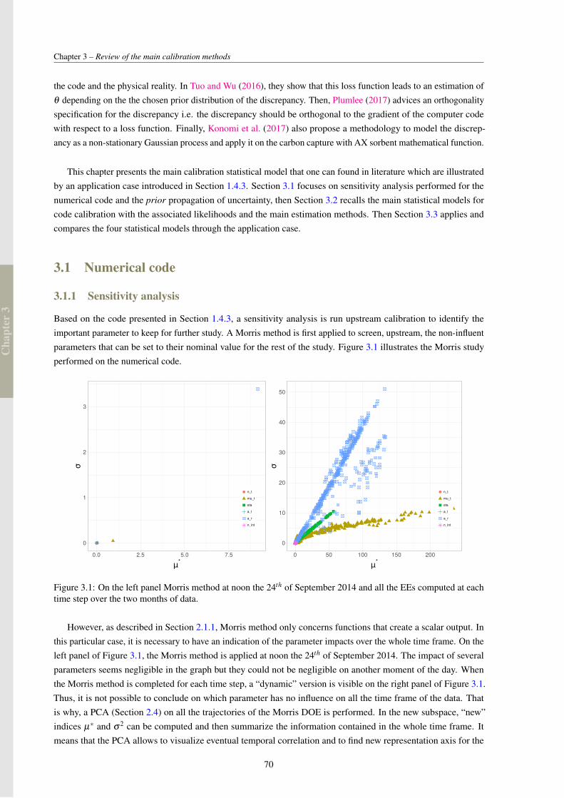
Cha

pter

3

Chapter 3 – Review of the main calibration methods

the code and the physical reality. In Tuo and Wu (2016), they show that this loss function leads to an estimation ofθ depending on the the chosen prior distribution of the discrepancy. Then, Plumlee (2017) advices an orthogonalityspecification for the discrepancy i.e. the discrepancy should be orthogonal to the gradient of the computer codewith respect to a loss function. Finally, Konomi et al. (2017) also propose a methodology to model the discrep-ancy as a non-stationary Gaussian process and apply it on the carbon capture with AX sorbent mathematical function.

This chapter presents the main calibration statistical model that one can found in literature which are illustratedby an application case introduced in Section 1.4.3. Section 3.1 focuses on sensitivity analysis performed for thenumerical code and the prior propagation of uncertainty, then Section 3.2 recalls the main statistical models forcode calibration with the associated likelihoods and the main estimation methods. Then Section 3.3 applies andcompares the four statistical models through the application case.

3.1 Numerical code

3.1.1 Sensitivity analysis

Based on the code presented in Section 1.4.3, a sensitivity analysis is run upstream calibration to identify theimportant parameter to keep for further study. A Morris method is first applied to screen, upstream, the non-influentparameters that can be set to their nominal value for the rest of the study. Figure 3.1 illustrates the Morris studyperformed on the numerical code.

0

1

2

3

0.0 2.5 5.0 7.5

μ*

σ

n_t

mu_t

eta

a_l

a_r

n_int

0

10

20

30

40

50

0 50 100 150 200

μ*

σ

n_t

mu_t

eta

a_l

a_r

n_int

Figure 3.1: On the left panel Morris method at noon the 24th of September 2014 and all the EEs computed at eachtime step over the two months of data.

However, as described in Section 2.1.1, Morris method only concerns functions that create a scalar output. Inthis particular case, it is necessary to have an indication of the parameter impacts over the whole time frame. On theleft panel of Figure 3.1, the Morris method is applied at noon the 24th of September 2014. The impact of severalparameters seems negligible in the graph but they could not be negligible on another moment of the day. Whenthe Morris method is completed for each time step, a “dynamic” version is visible on the right panel of Figure 3.1.Thus, it is not possible to conclude on which parameter has no influence on all the time frame of the data. Thatis why, a PCA (Section 2.4) on all the trajectories of the Morris DOE is performed. In the new subspace, “new”indices µ∗ and σ2 can be computed and then summarize the information contained in the whole time frame. Itmeans that the PCA allows to visualize eventual temporal correlation and to find new representation axis for the

70

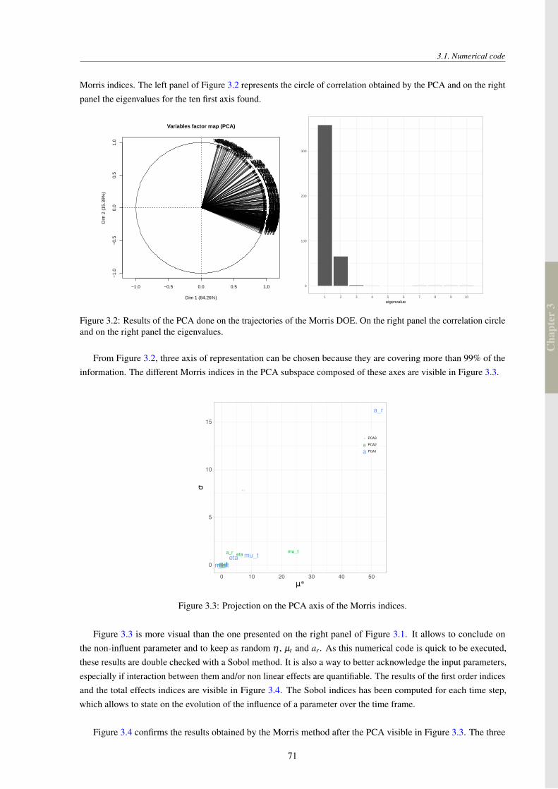
Cha

pter

3

3.1. Numerical code

Morris indices. The left panel of Figure 3.2 represents the circle of correlation obtained by the PCA and on the rightpanel the eigenvalues for the ten first axis found.

−1.0 −0.5 0.0 0.5 1.0

−1.

0−

0.5

0.0

0.5

1.0

Variables factor map (PCA)

Dim 1 (84.26%)

Dim

2 (

15.3

9%)

V1V2V3

V4

V5

V6V7V8

V9V10V11

V12

V13

V14V15V16V17V18V19V20V21

V22

V23

V24

V25V26V27

V28

V29

V30V31

V32V33V34

V35

V36V37V38

V39

V40

V41

V42V43

V44

V45V46V47V48V49V50

V51

V52

V53

V54V55

V56

V57V58

V59

V60V61V62

V63V64V65

V66

V67

V68V69

V70

V71V72

V73

V74

V75

V76V77V78V79V80V81V82V83V84V85V86V87V88V89V90

V91

V92

V93V94V95V96V97V98V99

V100

V101V102

V103

V104V105

V106

V107V108V109V110V111V112V113V114V115V116

V117V118

V119

V120

V121V122V123V124V125V126V127V128V129V130V131V132V133V134V135V136

V137V138

V139V140V141

V142V143V144

V145

V146

V147

V148

V149V150V151

V152

V153

V154

V155V156V157V158V159V160V161V162V163

V164

V165

V166

V167V168

V169V170V171V172V173V174

V175V176

V177

V178V179

V180

V181

V182V183

V184V185V186V187V188V189V190

V191V192V193

V194

V195

V196

V197

V198V199V200

V201V202

V203

V204

V205

V206

V207

V208

V209

V210

V211

V212

V213V214

V215V216V217

V218

V219

V220

V221V222

V223

V224

V225

V226V227V228V229V230V231V232V233V234

V235

V236V237

V238V239

V240

V241V242

V243V244

V245

V246V247

V248V249

V250

V251V252

V253

V254

V255V256

V257V258

V259

V260V261

V262

V263

V264V265

V266

V267

V268

V269V270

V271V272

V273

V274

V275

V276V277

V278

V279V280V281V282

V283V284V285V286V287

V288

V289

V290

V291V292V293

V294

V295V296V297

V298V299V300V301V302

V303V304

V305

V306

V307

V308

V309

V310

V311V312V313

V314V315

V316

V317

V318

V319

V320V321

V322

V323

V324V325V326V327V328V329V330

V331V332V333

V334V335V336V337V338V339V340V341V342V343V344V345V346V347V348V349

V350

V351

V352

V353

V354V355V356V357V358V359V360

V361

V362V363

V364V365V366V367V368V369V370V371V372V373V374V375

V376

V377

V378

V379

V380V381

V382V383V384V385

V386

V387

V388

V389

V390V391

V392

V393

V394

V395V396V397

V398V399

V400

V401

V402

V403

V404

V405

V406V407V408V409V410V411

V412V413

V414

V415V416

V417

V418

V419V420

V421V422

V423

V424V425

0

100

200

300

1 2 3 4 5 6 7 8 9 10

eigenvalue

Figure 3.2: Results of the PCA done on the trajectories of the Morris DOE. On the right panel the correlation circleand on the right panel the eigenvalues.

From Figure 3.2, three axis of representation can be chosen because they are covering more than 99% of theinformation. The different Morris indices in the PCA subspace composed of these axes are visible in Figure 3.3.

n_tmu_tetaa_l

a_r

n_intn_t

mu_teta

a_l

a_r

n_intn_tmu_teta

a_l

a_r

n_int0

5

10

15

0 10 20 30 40 50μ*

σ

a

aa

PCA3

PCA2

PCA1

Figure 3.3: Projection on the PCA axis of the Morris indices.

Figure 3.3 is more visual than the one presented on the right panel of Figure 3.1. It allows to conclude onthe non-influent parameter and to keep as random η , µt and ar. As this numerical code is quick to be executed,these results are double checked with a Sobol method. It is also a way to better acknowledge the input parameters,especially if interaction between them and/or non linear effects are quantifiable. The results of the first order indicesand the total effects indices are visible in Figure 3.4. The Sobol indices has been computed for each time step,which allows to state on the evolution of the influence of a parameter over the time frame.

Figure 3.4 confirms the results obtained by the Morris method after the PCA visible in Figure 3.3. The three

71

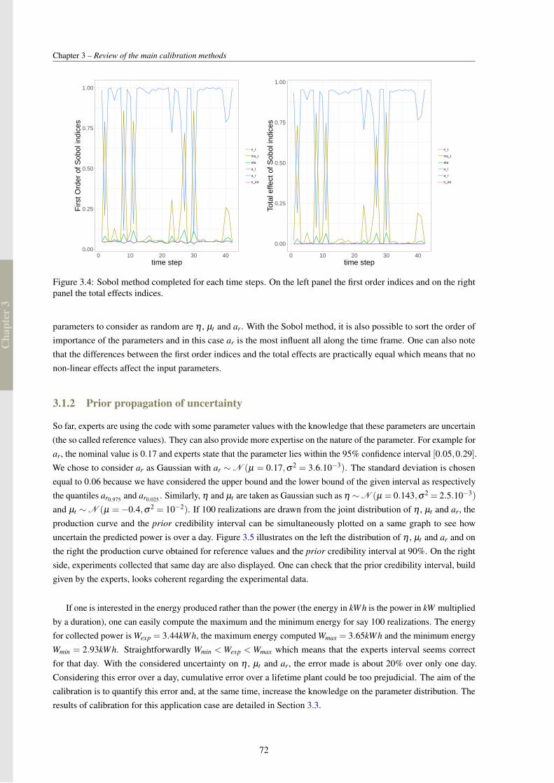
Cha

pter

3

Chapter 3 – Review of the main calibration methods

0.00

0.25

0.50

0.75

1.00

0 10 20 30 40time step

Firs

t Ord

er o

f Sob

ol in

dice

s

n_t

mu_t

eta

a_l

a_r

n_int

0.00

0.25

0.50

0.75

1.00

0 10 20 30 40time step

Tota

l effe

ct o

f Sob

ol in

dice

s

n_t

mu_t

eta

a_l

a_r

n_int

Figure 3.4: Sobol method completed for each time steps. On the left panel the first order indices and on the rightpanel the total effects indices.

parameters to consider as random are η , µt and ar. With the Sobol method, it is also possible to sort the order ofimportance of the parameters and in this case ar is the most influent all along the time frame. One can also notethat the differences between the first order indices and the total effects are practically equal which means that nonon-linear effects affect the input parameters.

3.1.2 Prior propagation of uncertainty

So far, experts are using the code with some parameter values with the knowledge that these parameters are uncertain(the so called reference values). They can also provide more expertise on the nature of the parameter. For example forar, the nominal value is 0.17 and experts state that the parameter lies within the 95% confidence interval [0.05,0.29].We chose to consider ar as Gaussian with ar ∼N (µ = 0.17,σ2 = 3.6.10−3). The standard deviation is chosenequal to 0.06 because we have considered the upper bound and the lower bound of the given interval as respectivelythe quantiles ar0.975 and ar0.025 . Similarly, η and µt are taken as Gaussian such as η ∼N (µ = 0.143,σ2 = 2.5.10−3)

and µt ∼N (µ =−0.4,σ2 = 10−2). If 100 realizations are drawn from the joint distribution of η , µt and ar, theproduction curve and the prior credibility interval can be simultaneously plotted on a same graph to see howuncertain the predicted power is over a day. Figure 3.5 illustrates on the left the distribution of η , µt and ar and onthe right the production curve obtained for reference values and the prior credibility interval at 90%. On the rightside, experiments collected that same day are also displayed. One can check that the prior credibility interval, buildgiven by the experts, looks coherent regarding the experimental data.

If one is interested in the energy produced rather than the power (the energy in kWh is the power in kW multipliedby a duration), one can easily compute the maximum and the minimum energy for say 100 realizations. The energyfor collected power is Wexp = 3.44kWh, the maximum energy computed Wmax = 3.65kWh and the minimum energyWmin = 2.93kWh. Straightforwardly Wmin < Wexp < Wmax which means that the experts interval seems correctfor that day. With the considered uncertainty on η , µt and ar, the error made is about 20% over only one day.Considering this error over a day, cumulative error over a lifetime plant could be too prejudicial. The aim of thecalibration is to quantify this error and, at the same time, increase the knowledge on the parameter distribution. Theresults of calibration for this application case are detailed in Section 3.3.

72

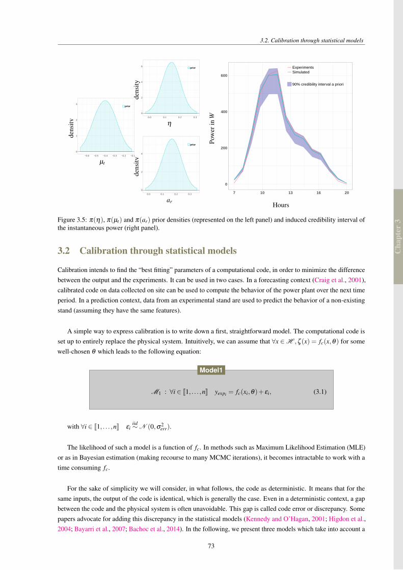
Cha

pter

3

3.2. Calibration through statistical models

0

2

4

6

0.0 0.1 0.2 0.3

prior

dens

ity

η

dens

ity

0

1

2

3

−0.6 −0.5 −0.4 −0.3 −0.2 −0.1

prior

µt

dens

ity

0

2

4

0.0 0.1 0.2 0.3

prior

ar

Pow

erin

W

0

200

400

600

7 10 13 16 20

ExperimentsSimulated

90% credibility interval a priori

Hours

Figure 3.5: π(η), π(µt) and π(ar) prior densities (represented on the left panel) and induced credibility interval ofthe instantaneous power (right panel).

3.2 Calibration through statistical models

Calibration intends to find the “best fitting” parameters of a computational code, in order to minimize the differencebetween the output and the experiments. It can be used in two cases. In a forecasting context (Craig et al., 2001),calibrated code on data collected on site can be used to compute the behavior of the power plant over the next timeperiod. In a prediction context, data from an experimental stand are used to predict the behavior of a non-existingstand (assuming they have the same features).

A simple way to express calibration is to write down a first, straightforward model. The computational code isset up to entirely replace the physical system. Intuitively, we can assume that ∀x ∈H ,ζ (x) = fc(x,θ) for somewell-chosen θ which leads to the following equation:

M1 : ∀i ∈ J1, . . . ,nK yexpi = fc(xi,θ)+ εi, (3.1)

Model1

with ∀i ∈ J1, . . . ,nK εiiid∼N (0,σ2

err).

The likelihood of such a model is a function of fc. In methods such as Maximum Likelihood Estimation (MLE)or as in Bayesian estimation (making recourse to many MCMC iterations), it becomes intractable to work with atime consuming fc.

For the sake of simplicity we will consider, in what follows, the code as deterministic. It means that for thesame inputs, the output of the code is identical, which is generally the case. Even in a deterministic context, a gapbetween the code and the physical system is often unavoidable. This gap is called code error or discrepancy. Somepapers advocate for adding this discrepancy in the statistical models (Kennedy and O’Hagan, 2001; Higdon et al.,2004; Bayarri et al., 2007; Bachoc et al., 2014). In the following, we present three models which take into account a

73

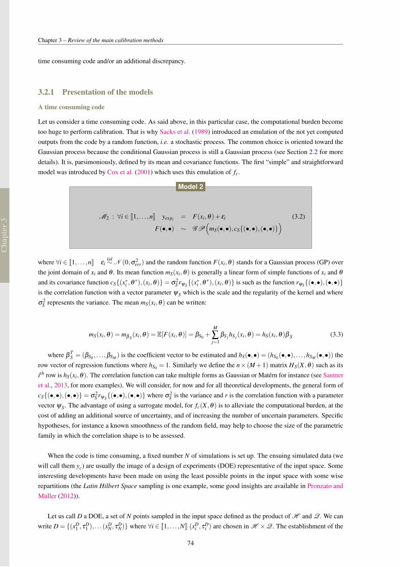
Cha

pter

3

Chapter 3 – Review of the main calibration methods

time consuming code and/or an additional discrepancy.

3.2.1 Presentation of the models

A time consuming code

Let us consider a time consuming code. As said above, in this particular case, the computational burden becometoo huge to perform calibration. That is why Sacks et al. (1989) introduced an emulation of the not yet computedoutputs from the code by a random function, i.e. a stochastic process. The common choice is oriented toward theGaussian process because the conditional Gaussian process is still a Gaussian process (see Section 2.2 for moredetails). It is, parsimoniously, defined by its mean and covariance functions. The first “simple” and straightforwardmodel was introduced by Cox et al. (2001) which uses this emulation of fc.

M2 : ∀i ∈ J1, . . . ,nK yexpi = F(xi,θ)+ εi (3.2)

F(•,•) ∼ G P(

mS(•,•),cS(•,•),(•,•))

Model 2

where ∀i ∈ J1, . . . ,nK εiiid∼N (0,σ2

err) and the random function F(xi,θ) stands for a Gaussian process (GP) overthe joint domain of xi and θ . Its mean function mS(xi,θ) is generally a linear form of simple functions of xi and θ

and its covariance function cS(x∗i ,θ ∗),(xi,θ)= σ2S rψS(x

∗i ,θ∗),(xi,θ) is such as the function rψS(•,•),(•,•)

is the correlation function with a vector parameter ψS which is the scale and the regularity of the kernel and whereσ2

S represents the variance. The mean mS(xi,θ) can be written:

mS(xi,θ) = mβ S(xi,θ) = E[F(xi,θ)] = βS0 +

M

∑j=1

βS j hS j(xi,θ) = hS(xi,θ)β S (3.3)

where βTS = (βS0 , . . . ,βSM ) is the coefficient vector to be estimated and hS(•,•) = (hS0(•,•), . . . ,hSM (•,•)) the

row vector of regression functions where hS0 = 1. Similarly we define the n× (M+1) matrix HS(X ,θ) such as itsith row is hS(xi,θ). The correlation function can take multiple forms as Gaussian or Matérn for instance (see Santneret al., 2013, for more examples). We will consider, for now and for all theoretical developments, the general form ofcS(•,•),(•,•)= σ2

S rψS(•,•),(•,•) where σ2S is the variance and r is the correlation function with a parameter

vector ψS. The advantage of using a surrogate model, for fc(X ,θ) is to alleviate the computational burden, at thecost of adding an additional source of uncertainty, and of increasing the number of uncertain parameters. Specifichypotheses, for instance a known smoothness of the random field, may help to choose the size of the parametricfamily in which the correlation shape is to be assessed.

When the code is time consuming, a fixed number N of simulations is set up. The ensuing simulated data (wewill call them yc) are usually the image of a design of experiments (DOE) representative of the input space. Someinteresting developments have been made on using the least possible points in the input space with some wiserepartitions (the Latin Hilbert Space sampling is one example, some good insights are available in Pronzato andMüller (2012)).

Let us call D a DOE, a set of N points sampled in the input space defined as the product of H and Q. We canwrite D = (xD

1 ,τD1 ), . . .(x

DN ,τ

DN) where ∀i ∈ J1, . . . ,NK (xD

i ,τDi ) are chosen in H ×Q. The establishment of the

74

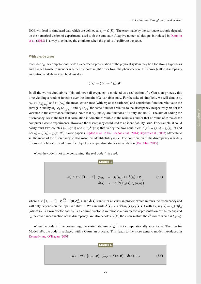
Cha

pter

3

3.2. Calibration through statistical models

DOE will lead to simulated data which are defined as yc = fc(D). The error made by the surrogate strongly dependson the numerical design of experiments used to fit the emulator. Adaptive numerical designs introduced in Damblinet al. (2018) is a way to enhance the emulator when the goal is to calibrate the code.

With a code error

Considering the computational code as a perfect representation of the physical system may be a too strong hypothesisand it is legitimate to wonder whether the code might differ from the phenomenon. This error (called discrepancyand introduced above) can be defined as:

δ (xi) = ζ (xi)− fc(xi,θ).

In all the works cited above, this unknown discrepancy is modeled as a realization of a Gaussian process, thistime yielding a random function over the domain of X variables only. For the sake of simplicity we will denote byms, cS (c

σ2S ,ψS

) and rS (rψS ) the mean, covariance (with σ2S as the variance) and correlation function relative to the

surrogate and by mδ , cδ (cσ2

δ,ψδ

) and rδ (rψδ) the same functions relative to the discrepancy (respectively σ2

δfor the

variance in the covariance function). Note that mδ and cδ are functions of x only and not θ . The aim of adding thediscrepancy lies in the fact that correlation is sometimes visible in the residuals and/or that no value of θ makes thecomputer close to experiments. However, the discrepancy could lead to an identifiability issue. For example, it couldeasily exist two couples (θ ,δ (xi)) and (θ ∗,δ ∗(xi)) that verify the two equalities: δ (xi) = ζ (xi)− fc(xi,θ) andδ ∗(xi) = ζ (xi)− fc(xi,θ

∗). Some papers (Higdon et al., 2004; Bachoc et al., 2014; Bayarri et al., 2007) advocate toset the mean of the discrepancy to 0 to solve this identifiability issue. The contribution of the discrepancy is widelydiscussed in literature and make the object of comparative studies in validation (Damblin, 2015).

When the code is not time consuming, the real code fc is used:

M3 : ∀i ∈ J1, . . . ,nK yexpi = fc(xi,θ)+δ (xi)+ εi (3.4)

δ (•) ∼ G P(

mδ (•),cδ (•,•))

Model 3

where ∀i ∈ J1, . . . ,nK εiiid∼N (0,σ2

err), and δ (•) stands for a Gaussian process which mimics the discrepancy andwill only depends on the input variables x. We can write δ (•)∼ G P(mδ (•),cδ (•,•)) with ∀x, mδ (x) = hδ (x)β δ

(where hδ is a row vector and β δ is a column vector if we choose a parametric representation of the mean) andcδ the covariance function of the discrepancy. We also denote Hδ (X) the n row matrix, the ith row of which is hδ (xi).

When the code is time consuming, the systematic use of fc is not computationally acceptable. Then, as forModel M2, the code is replaced with a Gaussian process. This leads to the more generic model introduced inKennedy and O’Hagan (2001).

M4 : ∀i ∈ J1, . . . ,nK yexpi = F(xi,θ)+δ (xi)+ εi (3.5)

Model 4

75

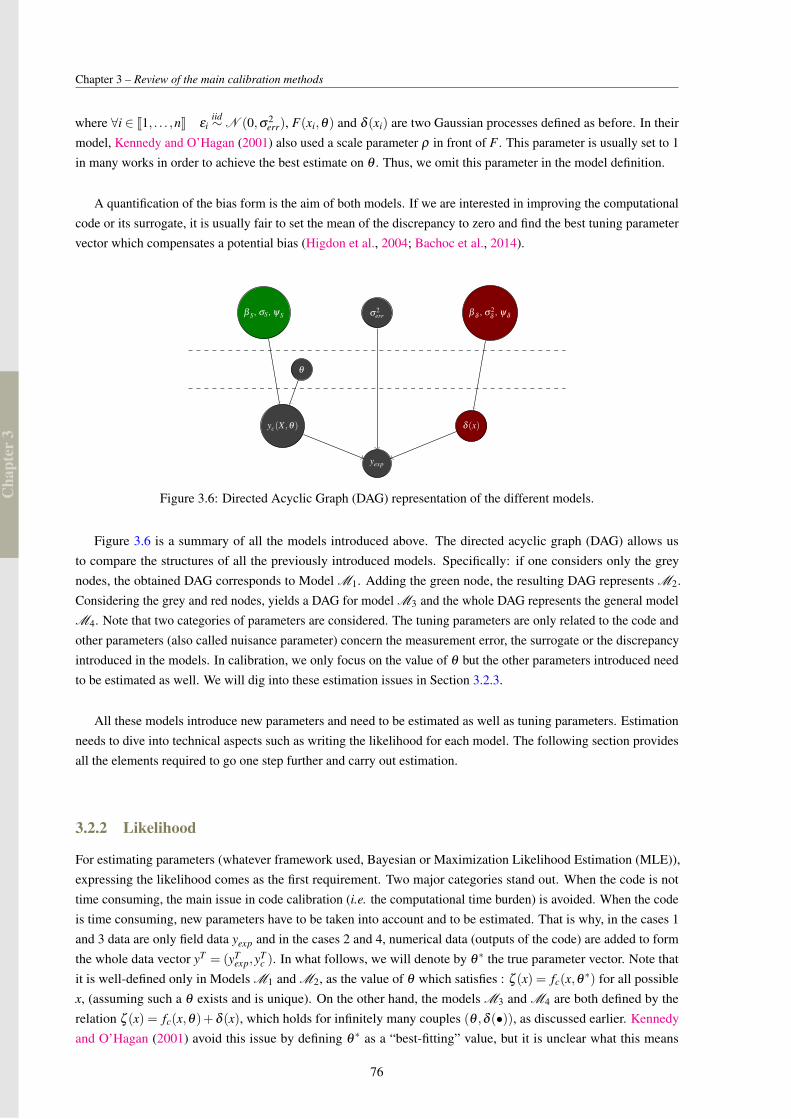
Cha

pter

3

Chapter 3 – Review of the main calibration methods

where ∀i ∈ J1, . . . ,nK εiiid∼N (0,σ2

err), F(xi,θ) and δ (xi) are two Gaussian processes defined as before. In theirmodel, Kennedy and O’Hagan (2001) also used a scale parameter ρ in front of F . This parameter is usually set to 1in many works in order to achieve the best estimate on θ . Thus, we omit this parameter in the model definition.

A quantification of the bias form is the aim of both models. If we are interested in improving the computationalcode or its surrogate, it is usually fair to set the mean of the discrepancy to zero and find the best tuning parametervector which compensates a potential bias (Higdon et al., 2004; Bachoc et al., 2014).

yexp

yc(X ,θ)

σ 2err

θ

β δ , σ 2δ

, ψδβ S , σS , ψS

δ (x)

Figure 3.6: Directed Acyclic Graph (DAG) representation of the different models.

Figure 3.6 is a summary of all the models introduced above. The directed acyclic graph (DAG) allows usto compare the structures of all the previously introduced models. Specifically: if one considers only the greynodes, the obtained DAG corresponds to Model M1. Adding the green node, the resulting DAG represents M2.Considering the grey and red nodes, yields a DAG for model M3 and the whole DAG represents the general modelM4. Note that two categories of parameters are considered. The tuning parameters are only related to the code andother parameters (also called nuisance parameter) concern the measurement error, the surrogate or the discrepancyintroduced in the models. In calibration, we only focus on the value of θ but the other parameters introduced needto be estimated as well. We will dig into these estimation issues in Section 3.2.3.

All these models introduce new parameters and need to be estimated as well as tuning parameters. Estimationneeds to dive into technical aspects such as writing the likelihood for each model. The following section providesall the elements required to go one step further and carry out estimation.

3.2.2 Likelihood

For estimating parameters (whatever framework used, Bayesian or Maximization Likelihood Estimation (MLE)),expressing the likelihood comes as the first requirement. Two major categories stand out. When the code is nottime consuming, the main issue in code calibration (i.e. the computational time burden) is avoided. When the codeis time consuming, new parameters have to be taken into account and to be estimated. That is why, in the cases 1and 3 data are only field data yexp and in the cases 2 and 4, numerical data (outputs of the code) are added to formthe whole data vector yT = (yT

exp,yTc ). In what follows, we will denote by θ

∗ the true parameter vector. Note thatit is well-defined only in Models M1 and M2, as the value of θ which satisfies : ζ (x) = fc(x,θ ∗) for all possiblex, (assuming such a θ exists and is unique). On the other hand, the models M3 and M4 are both defined by therelation ζ (x) = fc(x,θ)+δ (x), which holds for infinitely many couples (θ ,δ (•)), as discussed earlier. Kennedyand O’Hagan (2001) avoid this issue by defining θ

∗ as a “best-fitting” value, but it is unclear what this means

76

Cha

pter

3

3.2. Calibration through statistical models

exactly (see the discussion section of their paper for further details).

In order to simplify the notation, we will use for the rest of the paper Φ = σ2S ,σ

2δ,ψS,ψδ and ΦS = σ2

S ,ψSand Φδ = σ2

δ,ψδ, where σ2

S and σ2δ

are the variances of the two Gaussian processes respectively relative to thesurrogate and the discrepancy. The two parameter vectors ψS and ψδ are relative to the correlation functions. Letus call β

T = (β TS ,β

Tδ ) the vector of collected coefficient vectors.

Both cases of time consuming or not time consuming code will be dealt with. The likelihood equations willbe written for the generic forms of M3 and M4. The likelihoods for the simpler models M1 and M2 will be thenderived since M1 ⊂M3 and M2 ⊂M4.

A fast code

The generic model which deals with calibration with a code quick to run is detailed in Equation (3.4). Experimentaldata are the only one needed because simulation data are free but will not bring additional information for theparameters of Model M3. Experimental data follow a Gaussian distribution, the expectation of which is:

E[yexp|θ ,β δ ;X ] = mβ δexp(X ,θ) = mexp(X ,θ) = fc(X ,θ)+Hδ (X)β δ .

Then, the expression of the variance is given by:

Var[yexp|Φδ ;X ] =V Φδ ,σ2err

exp (X) =V exp(X) = Σδ (X)+σ2errIn

with ∀(i, j) ∈ J1, . . . ,nK2 : (Σδ (X))i, j = (ΣΦδ

δ(X))i, j = cδ (xi,x j). The likelihood in this particular case can be

written as

L F(θ ,β δ ,Φδ ;yexp,X) =1

(2π)n/2|V exp(X)|1/2 exp

− 1

2

(yexp−mexp(X ,θ)

)TV exp(X)−1

(yexp−mexp(X ,θ)

).

(3.6)

This likelihood is relative to Model M3 (Equation (3.4)). For the specific case, where no discrepancy isconsidered (corresponding to M1 Equation (3.1)) the likelihood can be written in a similar way but with mexp(X ,θ)=

fc(X ,θ) and V exp(X) = σ2errIn. Note that the covariance matrix depends only on σerr

2. It implies that if we seek toestimate the posterior density on θ (in a Bayesian framework), this covariance term is superfluous.

Then the likelihood can be rewritten in an simpler way:

L F(θ ,σ2err;yexp,X) =

1(2π)n/2σn

errexp

− 1

2σ2err||yexp− fc(X ,θ)||22

. (3.7)

The models using the code with or without the discrepancy do look quite similar. For theoretical development,it might be easier to work with the one without discrepancy. From an experimental point of view, it could beinteresting to study the role of the code error.

77

Cha

pter

3

Chapter 3 – Review of the main calibration methods

A time consuming code

When a code is time consuming and replaced by a surrogate, additional parameters are to be estimated. As introducedabove, a DOE is set up and intends to be a representative sample of the input space (variable and parameter inputspace). Simulated data from this DOE (called yc) will constitute additional data for the estimation of the nuisanceparameters. Depending on how we consider that two sources of data are linked, multiple likelihoods can be set up.For the theoretical development, we will consider the general model M4 and we will detail the particular case M2

hereafter.

The first likelihood useful in estimation is the full likelihood. This one concerns the distribution of allcollected data (yT = (yT

exp,yTc )). That means, we are interested in estimating the parameters of the distribu-

tion π(y|θ ,β ,Φ,σ2err;X ,D) which is Gaussian. The expectations can be written from both expectancies of

π(yexp|θ ,β ,Φ,σ2err;X) and π(yc|θ ,β S,ΦS;X).E[yc|β S;D] = mβ S

c (D) = mc(D) = HS(D)β S

E[yexp|θ ,β ;X ] = mβexp(X ,θ) = mexp(X ,θ) = HS(X ,θ)β S +Hδ (X)β δ

(3.8)

This can be summed up for two component vectors yT = (yTexp,y

Tc ):

E[y|θ ,β ;X ,D] = mβy ((X ,θ),D) = my((X ,θ),D) = H((X ,θ),D)β

=

(HS(X ,θ) Hδ (X)

HS(D) 0

)β .

(3.9)

The variance matrix now includes the covariance functions of the discrepancy and the surrogate.

Var[y|θ ,Φ,σ2err;X ,D] =V Φ,σ2

err((X ,θ),D) =V ((X ,θ),D)

=

(Σexp,exp(X ,θ)+Σδ (X)+σ2

errIn Σexp,c((X ,θ),D)

Σexp,c((X ,θ),D)T Σc,c(D)

)(3.10)

where

• ∀(i, j) ∈ J1, . . . ,nK2 : (Σexp,exp(X ,θ))i, j = cS(xi,θ),(x j,θ),

• ∀(i, j) ∈ J1, . . . ,nK× J1, . . . ,NK : (Σexp,c((X ,θ),D))i, j = cS(xi,θ i),(xDj ,τ

Dj ),

• ∀(i, j) ∈ J1, . . . ,nK2 : (Σδ (X))i, j = cδ(xi,x j),

• ∀(i, j) ∈ J1, . . . ,NK2 : (Σc,c(D))i, j = cS(xDi ,τ

Di ),(x

Dj ,τ

Dj ).

As a reminder D is the DOE set up to build the surrogate and is defined as D = (xD1 ,τ

D1 ), . . .(x

DN ,τ

DN). The

general expression of the full likelihood can then be expressed:

L F(θ ,β ,Φ,σ2err;y,X ,D) =

1(2π)(n+N)/2|V ((X ,θ),D)|1/2 exp

− 1

2

(y−my((X ,θ),D)

)T

V ((X ,θ),D)−1(

y−my((X ,θ),D))

.

(3.11)

78

Cha

pter

3

3.2. Calibration through statistical models

The particular cases of Bayarri et al. (2007) and Higdon et al. (2004) a zero mean for the discrepancy is

considered. Under this condition, we have my((X ,θ),D) =

(HS(X ,θ)

HS(D)

)β S and the other terms remain the same.

For the model M2 where a surrogate is used without any discrepancy (Cox et al., 2001), the expectation becomes:

E[y|θ ,β S;X ,D] = my((X ,θ),D) = H((X ,θ),D)β S =

(HS(X ,θ)

HS(D)

)β S (3.12)

and the covariance:

Var[y|θ ,Φ,σ2err;X ,D] =V ((X ,θ),D) =

(Σexp,exp(X ,θ)+σ2

errIn Σexp,c((X ,θ),D)

Σexp,c((X ,θ),D)T Σc,c(D)

)(3.13)

where covariances matrices are the same as defined before.

The estimation can be separate into different steps where the partial likelihood (Equation (3.14)) could be useful.This one only concerns simulated data and the corresponding surrogate. The partial likelihoods of the model M2

and M4 are then the same. That means we are only interesting in estimating the distribution π(β S,ΦS|yc) whereΦS = σ2

S ,ψS. The expectation can be obtained by considering only the mean function of the surrogate (Equation(3.8)) and the variance is straightforwardly linked to the variance of the surrogate.

Var[yc|ΦS;D] =V ΦSc (D) =V c(D) = Σc,c(D),

where ∀(i, j) ∈ [1, . . . ,N]2 : (Σc,c(D))i, j = cS(xDi ,θ

Di ),(x

Dj ,θ

Dj ). Let us recall that Equation (3.8) established

that mc(D) = HS(D)β S. It implies that the partial likelihood relative to M4 and M2 is:

L M(β S,ΦS;yc,D) =1

(2π)N/2|V c(D)|1/2 exp

− 1

2

(yc−mc(D)

)TV c(D)−1

(yc−mc(D)

). (3.14)

As the other model introduced by Higdon et al. (2004) and Bayarri et al. (2007) only deals with changes on thediscrepancy, the partial likelihood remains identical as the one for the model in Bayarri et al. (2007).

From what has been introduced before, one can write the conditional distribution π(yexp|yc) (see Section 2.2 formore details) from the joint distribution π(yexp,yc) and for M4:(

yexp

yc

)∼N

((mexp(X ,θ)

mc(D)

),

(Σexp,exp(X ,θ)+Σδ +σ2

errIn Σexp,c((X ,θ),D)

Σexp,c((X ,θ),D)T Σc,c(D)

))where mc and mexp are defined Equation (3.8) and covariance matrices defined above before Equation (3.11). Then,

yexp|yc ∼N (µexp|c((X ,θ),D),Σexp|c((X ,θ),D))

with:

µexp|c((X ,θ),D) = mexp(X ,θ)+Σexp,c((X ,θ),D)Σc,c(D)−1(yc−mc(D)), (3.15)

Σexp|c((X ,θ),D) = Σexp,exp(X ,θ)+Σδ +σ2errIn−Σexp,c((X ,θ),D)Σc,c(D)−1

Σexp,c((X ,θ),D)T . (3.16)

For M2, the variance term Σexp,exp(X ,θ)+Σδ +σ2errIn in Equation (3.2.2) becomes Σexp,exp(X ,θ)+σ2

errIn

because there is no discrepancy. It means that Σexp|c((X ,θ),D) for M2 can be rewritten as:

79

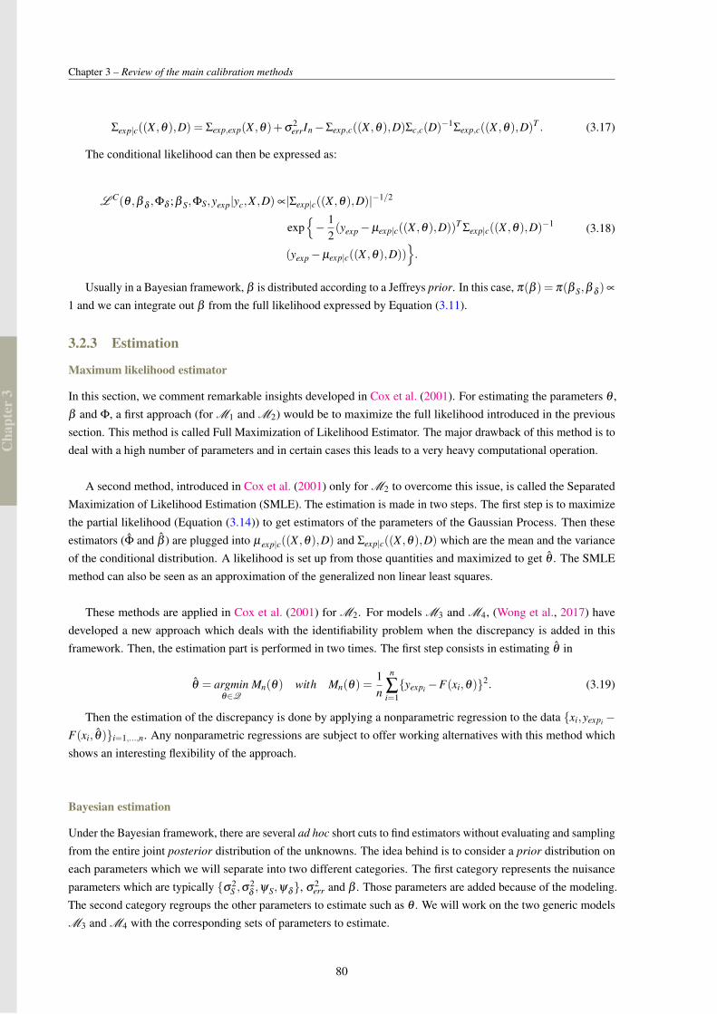
Cha

pter

3

Chapter 3 – Review of the main calibration methods

Σexp|c((X ,θ),D) = Σexp,exp(X ,θ)+σ2errIn−Σexp,c((X ,θ),D)Σc,c(D)−1

Σexp,c((X ,θ),D)T . (3.17)

The conditional likelihood can then be expressed as:

L C(θ ,β δ ,Φδ ;β S,ΦS,yexp|yc,X ,D) ∝|Σexp|c((X ,θ),D)|−1/2

exp− 1

2(yexp−µexp|c((X ,θ),D))T

Σexp|c((X ,θ),D)−1

(yexp−µexp|c((X ,θ),D)).

(3.18)

Usually in a Bayesian framework, β is distributed according to a Jeffreys prior. In this case, π(β ) = π(β S,β δ )∝

1 and we can integrate out β from the full likelihood expressed by Equation (3.11).

3.2.3 Estimation

Maximum likelihood estimator

In this section, we comment remarkable insights developed in Cox et al. (2001). For estimating the parameters θ ,β and Φ, a first approach (for M1 and M2) would be to maximize the full likelihood introduced in the previoussection. This method is called Full Maximization of Likelihood Estimator. The major drawback of this method is todeal with a high number of parameters and in certain cases this leads to a very heavy computational operation.

A second method, introduced in Cox et al. (2001) only for M2 to overcome this issue, is called the SeparatedMaximization of Likelihood Estimation (SMLE). The estimation is made in two steps. The first step is to maximizethe partial likelihood (Equation (3.14)) to get estimators of the parameters of the Gaussian Process. Then theseestimators (Φ and β ) are plugged into µexp|c((X ,θ),D) and Σexp|c((X ,θ),D) which are the mean and the varianceof the conditional distribution. A likelihood is set up from those quantities and maximized to get θ . The SMLEmethod can also be seen as an approximation of the generalized non linear least squares.

These methods are applied in Cox et al. (2001) for M2. For models M3 and M4, (Wong et al., 2017) havedeveloped a new approach which deals with the identifiability problem when the discrepancy is added in thisframework. Then, the estimation part is performed in two times. The first step consists in estimating θ in

θ = argminθ∈Q

Mn(θ) with Mn(θ) =1n

n

∑i=1yexpi −F(xi,θ)2. (3.19)

Then the estimation of the discrepancy is done by applying a nonparametric regression to the data xi,yexpi −F(xi, θ)i=1,...,n. Any nonparametric regressions are subject to offer working alternatives with this method whichshows an interesting flexibility of the approach.

Bayesian estimation

Under the Bayesian framework, there are several ad hoc short cuts to find estimators without evaluating and samplingfrom the entire joint posterior distribution of the unknowns. The idea behind is to consider a prior distribution oneach parameters which we will separate into two different categories. The first category represents the nuisanceparameters which are typically σ2

S ,σ2δ,ψS,ψδ, σ2

err and β . Those parameters are added because of the modeling.The second category regroups the other parameters to estimate such as θ . We will work on the two generic modelsM3 and M4 with the corresponding sets of parameters to estimate.

80

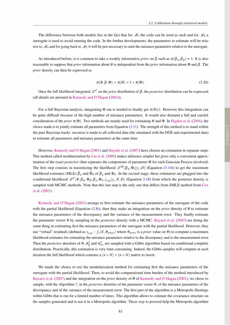
Cha

pter

3

3.2. Calibration through statistical models

The difference between both models lies in the fact that for M3 the code can be used as such and for M4 asurrogate is used to avoid running the code. In the further developments, the parameters to estimate will be rela-tive to M4 and for going back to M3 it will be just necessary to omit the nuisance parameters relative to the surrogate.

As introduced before, it is common to take a weakly informative prior on β such as π(β S,β δ ) ∝ 1. It is alsoreasonable to suppose that prior information about θ is independent from the prior information about Φ and β . Theprior density can then be expressed as

π(θ ,β ,Φ) = π(θ)×1×π(Φ). (3.20)

Once the full likelihood integrated L F on the prior distribution of β , the posterior distribution can be expressed(all details are pursued in Kennedy and O’Hagan (2001)).

For a full Bayesian analysis, integrating Φ out is needed to finally get π(θ |y). However this integration canbe quite difficult because of the high number of nuisance parameters. It would also demand a full and carefulconsideration of the prior π(Φ). Two methods are mainly used for estimating θ and Φ. In Higdon et al. (2004), thechoice made is to jointly estimate all parameters from Equation (3.11). The strength of this method is to stand withinthe pure Bayesian tracks: recourse is made to all collected data (the simulated with the DOE and experimental data)to estimate all parameters and nuisance parameters at the same time.

However, Kennedy and O’Hagan (2001) and Bayarri et al. (2007) have chosen an estimation in separate steps.This method called modularization by Liu et al. (2009) makes inference simpler but gives only a convenient approx-imation of the exact posterior (that separates the components of parameter Φ for each Gaussian Process involved).The first step consists in maximizing the likelihood L M(β S,ΦS|yc;D) (Equation (3.14)) to get the maximumlikelihood estimates (MLE) β S and ΦS of β S and ΦS. In the second stage, these estimators are plugged into theconditional likelihood L C(θ ,β δ ,Φδ ;β S,ΦS,yexp|yc,X ,D) (Equation 3.18) from which the posterior density issampled with MCMC methods. Note that this last step is the only one that differs from SMLE method from Coxet al. (2001).

Kennedy and O’Hagan (2001) arrange to first estimate the nuisance parameters of the surrogate of the codewith the partial likelihood (Equation (3.8)), then they make an integration on the prior density of θ to estimatethe nuisance parameters of the discrepancy and the variance of the measurement error. They finally estimatethe parameter vector θ by sampling in the posterior density with a MCMC. Bayarri et al. (2007) are doing thesame thing in estimating first the nuisance parameters of the surrogate with the partial likelihood. However, theyuse “virtual” residuals (defined as yexp− fc(X ,θ prior) where θ prior is a prior value on θ ) to compute a maximumlikelihood estimates for estimating the nuisance parameters relative to the discrepancy and to the measurement error.Then the posterior densities of θ , σ2

δand σ2

err are sampled with a Gibbs algorithm based on conditional completedistribution. Practically, this estimation is very time consuming. Indeed, the Gibbs sampler will compute at eachiteration the full likelihood which contains a (n+N)× (n+N) matrix to invert.

We made the choice to use the modularization method for estimating first the nuisance parameters of thesurrogate with the partial likelihood. Then, to avoid the computational time burden of the method introduced byBayarri et al. (2007) and the integration on the prior density of θ of Kennedy and O’Hagan (2001), we chose tosample, with the Algorithm 7, in the posterior densities of the parameter vector θ , of the nuisance parameters of thediscrepancy and of the variance of the measurement error. The first part of the algorithm is a Metropolis Hastingswithin Gibbs that is run for a limited number of times. This algorithm allows to estimate the covariance structure onthe samples generated and to use it in a Metropolis algorithm. These way to proceed help the Metropolis algorithm

81

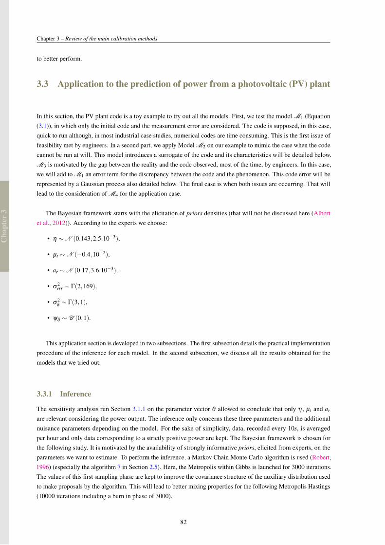
Cha

pter

3

Chapter 3 – Review of the main calibration methods

to better perform.

3.3 Application to the prediction of power from a photovoltaic (PV) plant

In this section, the PV plant code is a toy example to try out all the models. First, we test the model M1 (Equation(3.1)), in which only the initial code and the measurement error are considered. The code is supposed, in this case,quick to run although, in most industrial case studies, numerical codes are time consuming. This is the first issue offeasibility met by engineers. In a second part, we apply Model M2 on our example to mimic the case when the codecannot be run at will. This model introduces a surrogate of the code and its characteristics will be detailed below.M3 is motivated by the gap between the reality and the code observed, most of the time, by engineers. In this case,we will add to M1 an error term for the discrepancy between the code and the phenomenon. This code error will berepresented by a Gaussian process also detailed below. The final case is when both issues are occurring. That willlead to the consideration of M4 for the application case.

The Bayesian framework starts with the elicitation of priors densities (that will not be discussed here (Albertet al., 2012)). According to the experts we choose:

• η ∼N (0.143,2.5.10−3),

• µt ∼N (−0.4,10−2),

• ar ∼N (0.17,3.6.10−3),

• σ2err ∼ Γ(2,169),

• σ2δ∼ Γ(3,1),

• ψδ ∼U (0,1).

This application section is developed in two subsections. The first subsection details the practical implementationprocedure of the inference for each model. In the second subsection, we discuss all the results obtained for themodels that we tried out.

3.3.1 Inference

The sensitivity analysis run Section 3.1.1 on the parameter vector θ allowed to conclude that only η , µt and ar

are relevant considering the power output. The inference only concerns these three parameters and the additionalnuisance parameters depending on the model. For the sake of simplicity, data, recorded every 10s, is averagedper hour and only data corresponding to a strictly positive power are kept. The Bayesian framework is chosen forthe following study. It is motivated by the availability of strongly informative priors, elicited from experts, on theparameters we want to estimate. To perform the inference, a Markov Chain Monte Carlo algorithm is used (Robert,1996) (especially the algorithm 7 in Section 2.5). Here, the Metropolis within Gibbs is launched for 3000 iterations.The values of this first sampling phase are kept to improve the covariance structure of the auxiliary distribution usedto make proposals by the algorithm. This will lead to better mixing properties for the following Metropolis Hastings(10000 iterations including a burn in phase of 3000).

82

Cha

pter

3

3.3. Application to the prediction of power from a photovoltaic (PV) plant

Two months of data are studied. The PV production over August and September 2014 are available. We usedthose two months of data averaged per hour which makes 1019 points. For the cross validation, three days ofinstantaneous power (51 points) are taken off the learning set and used to evaluate the predictive power of the modelconsidering the rest of the available data.

The Gaussian process

As said in Section 1.4.3, 6 input variables are needed to run the code. These are t the UTC time, L the latitude, l

the longitude, Ig the global irradiation, Id the diffuse irradiation and Te the ambient temperature. The test stand isprecisely located. Therefore, the latitude and the longitude are not to be considered since they do not change byrecords.

The major issue in emulating the behavior of the code is to deal with correlated variables. Actually, the globalirradiation, diffuse irradiation and ambient temperature depend on the time which defines the sun position. If aspace filling DOE, is taken into [0,1]4 and then unnormalized between the upper and lower bounds of the 4 inputvariables and the parameter, some configurations tested would not make any sense. We could obtain for example, atime which indicates the morning and a global irradiation value which corresponds at noon. To solve this problem,we choose to run a PCA (Principle Component Analysis) on the matrix containing all the xi’s (over the durationused for the calibration). The aim is to access an uncorrelated space in which we could sample a DOE which wouldkeep a physical sense and then go back to the original space with the transformation matrix.

The main steps of this method are:

1. the PCA is performed on the matrix X where the ith line contains xi =

tiIgi

Idi

Tei

where xi ∈ R4,

2. the maximin LHS is sampled in the uncorrelated space given by the PCA,

3. the transformation matrix T allows us to go back in the original space,

4. the code is run for those points and gives the computed data yc.

The Gaussian processes emulated from this method reveal to work much better. We also could have developedthe method with an adaptive numerical design (see (Damblin et al., 2018)) to the correlated input variables.

To position the application case to a time consuming context, a limited number of experiments is allowed for theDOE which establishes the surrogate. We will limit the number of code calls to 50 to investigate the time consumingsituation and compare it to other situations more favorables. This number of experiments is taken when computercodes are extremely time consuming. To compare the quality of M2 with a DOE of 50 points, we chose to compareit with a model M2 established with a DOE of 100 points.

Table 3.1: Results in cross validation for M2 for 2 different DOE sizes

50 points 100 pointscoverage rate at 90% (in %) 32 65

RMSE of the instantaneous power (W ) 21.61 19.7

83

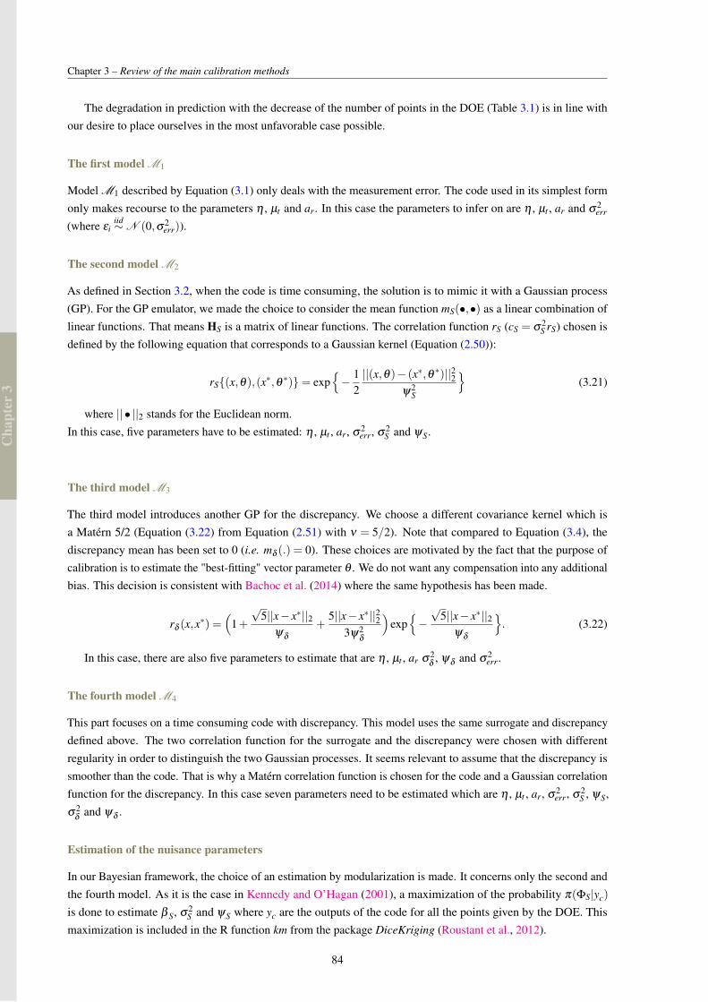
Cha

pter

3

Chapter 3 – Review of the main calibration methods

The degradation in prediction with the decrease of the number of points in the DOE (Table 3.1) is in line withour desire to place ourselves in the most unfavorable case possible.

The first model M1

Model M1 described by Equation (3.1) only deals with the measurement error. The code used in its simplest formonly makes recourse to the parameters η , µt and ar. In this case the parameters to infer on are η , µt , ar and σ2

err

(where εiiid∼N (0,σ2

err)).

The second model M2

As defined in Section 3.2, when the code is time consuming, the solution is to mimic it with a Gaussian process(GP). For the GP emulator, we made the choice to consider the mean function mS(•,•) as a linear combination oflinear functions. That means HS is a matrix of linear functions. The correlation function rS (cS = σ2

S rS) chosen isdefined by the following equation that corresponds to a Gaussian kernel (Equation (2.50)):

rS(x,θ),(x∗,θ ∗)= exp− 1

2||(x,θ)− (x∗,θ ∗)||22

ψ2S

(3.21)

where || • ||2 stands for the Euclidean norm.In this case, five parameters have to be estimated: η , µt , ar, σ2

err, σ2S and ψS.

The third model M3

The third model introduces another GP for the discrepancy. We choose a different covariance kernel which isa Matérn 5/2 (Equation (3.22) from Equation (2.51) with ν = 5/2). Note that compared to Equation (3.4), thediscrepancy mean has been set to 0 (i.e. mδ (.) = 0). These choices are motivated by the fact that the purpose ofcalibration is to estimate the "best-fitting" vector parameter θ . We do not want any compensation into any additionalbias. This decision is consistent with Bachoc et al. (2014) where the same hypothesis has been made.

rδ (x,x∗) =

(1+

√5||x− x∗||2

ψδ

+5||x− x∗||22

3ψ2δ

)exp−√

5||x− x∗||2ψδ

. (3.22)

In this case, there are also five parameters to estimate that are η , µt , ar σ2δ

, ψδ and σ2err.

The fourth model M4

This part focuses on a time consuming code with discrepancy. This model uses the same surrogate and discrepancydefined above. The two correlation function for the surrogate and the discrepancy were chosen with differentregularity in order to distinguish the two Gaussian processes. It seems relevant to assume that the discrepancy issmoother than the code. That is why a Matérn correlation function is chosen for the code and a Gaussian correlationfunction for the discrepancy. In this case seven parameters need to be estimated which are η , µt , ar, σ2

err, σ2S , ψS,

σ2δ

and ψδ .

Estimation of the nuisance parameters

In our Bayesian framework, the choice of an estimation by modularization is made. It concerns only the second andthe fourth model. As it is the case in Kennedy and O’Hagan (2001), a maximization of the probability π(ΦS|yc)

is done to estimate β S, σ2S and ψS where yc are the outputs of the code for all the points given by the DOE. This

maximization is included in the R function km from the package DiceKriging (Roustant et al., 2012).

84

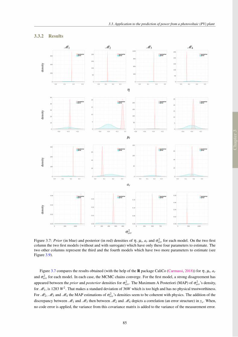
Cha

pter

3

3.3. Application to the prediction of power from a photovoltaic (PV) plant

3.3.2 Results

M1 M2 M3 M4

dens

ity

0

200

400

600

0.0 0.1 0.2 0.3

posteriorprior

0

50

100

150

200

0.0 0.1 0.2 0.3

posteriorprior

0

300

600

900

1200

0.0 0.1 0.2 0.3

posteriorprior

0

50

100

150

200

250

0.0 0.1 0.2 0.3

posteriorprior

η

dens

ity

0

10

20

30

40

50

−0.6 −0.4 −0.2

posteriorprior

0

5

10

15

20

−0.6 −0.4 −0.2 0.0

posteriorprior

0

50

100

150

200

−0.8 −0.6 −0.4 −0.2

posteriorprior

0

5

10

15

20

25

−0.6 −0.4 −0.2

posteriorprior

µt

dens

ity

0

100

200

300

0.0 0.1 0.2 0.3

posteriorprior

0

20

40

60

0.0 0.1 0.2 0.3

posteriorprior

0

50

100

150

0.0 0.1 0.2 0.3

posteriorprior

0

20

40

60

0.0 0.1 0.2 0.3

posteriorprior

ar

dens

ity

0.00

0.02

0.04

0.06

0 500 1000

posteriorprior

0.00

0.01

0.02

0.03

0 200 400 600 800

posteriorprior

0.00

0.05

0.10

0.15

0 250 500 750

posteriorprior

0.00

0.02

0.04

0.06

0.08

0 500 1000

posteriorprior

σ2err

Figure 3.7: Prior (in blue) and posterior (in red) densities of η , µt , ar and σ2err for each model. On the two first

column the two first models (without and with surrogate) which have only these four parameters to estimate. Thetwo other columns represent the third and the fourth models which have two more parameters to estimate (seeFigure 3.9).

Figure 3.7 compares the results obtained (with the help of the R package CaliCo (Carmassi, 2018)) for η , µt , ar

and σ2err for each model. In each case, the MCMC chains converge. For the first model, a strong disagreement has

appeared between the prior and posterior densities for σ2err. The Maximum A Posteriori (MAP) of σ2

err’s density,for M1, is 1283 W 2. That makes a standard deviation of 36W which is too high and has no physical trustworthiness.For M2, M3 and M4 the MAP estimations of σ2

err’s densities seem to be coherent with physics. The addition of thediscrepancy between M1 and M3 then between M2 and M4 depicts a correlation (an error structure) in ye. When,no code error is applied, the variance from this covariance matrix is added to the variance of the measurement error.

85

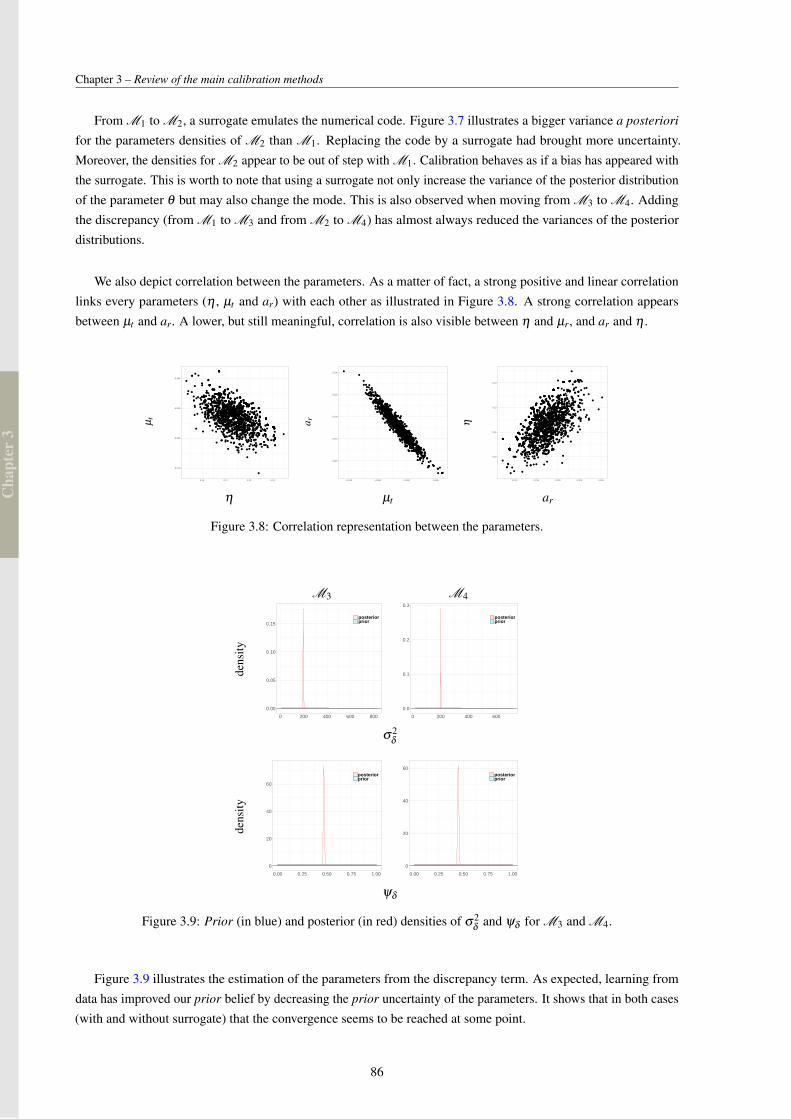
Cha

pter

3

Chapter 3 – Review of the main calibration methods

From M1 to M2, a surrogate emulates the numerical code. Figure 3.7 illustrates a bigger variance a posteriori

for the parameters densities of M2 than M1. Replacing the code by a surrogate had brought more uncertainty.Moreover, the densities for M2 appear to be out of step with M1. Calibration behaves as if a bias has appeared withthe surrogate. This is worth to note that using a surrogate not only increase the variance of the posterior distributionof the parameter θ but may also change the mode. This is also observed when moving from M3 to M4. Addingthe discrepancy (from M1 to M3 and from M2 to M4) has almost always reduced the variances of the posteriordistributions.

We also depict correlation between the parameters. As a matter of fact, a strong positive and linear correlationlinks every parameters (η , µt and ar) with each other as illustrated in Figure 3.8. A strong correlation appearsbetween µt and ar. A lower, but still meaningful, correlation is also visible between η and µr, and ar and η .

µt

−0.510

−0.505

−0.500

−0.495

0.10 0.11 0.12 0.13

a r

0.210

0.215

0.220

0.225

0.230

−0.510 −0.505 −0.500 −0.495

η

0.10

0.11

0.12

0.13

0.210 0.215 0.220 0.225 0.230

η µt ar

Figure 3.8: Correlation representation between the parameters.

M3 M4

dens

ity

0.00

0.05

0.10

0.15

0 200 400 600 800

posteriorprior

0.0

0.1

0.2

0.3

0 200 400 600

posteriorprior

σ2δ

dens

ity

0

20

40

60

0.00 0.25 0.50 0.75 1.00

posteriorprior

0

20

40

60

0.00 0.25 0.50 0.75 1.00

posteriorprior

ψδ

Figure 3.9: Prior (in blue) and posterior (in red) densities of σ2δ

and ψδ for M3 and M4.

Figure 3.9 illustrates the estimation of the parameters from the discrepancy term. As expected, learning fromdata has improved our prior belief by decreasing the prior uncertainty of the parameters. It shows that in both cases(with and without surrogate) that the convergence seems to be reached at some point.

86

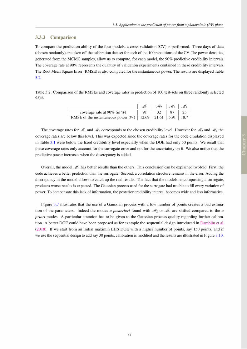
Cha

pter

3

3.3. Application to the prediction of power from a photovoltaic (PV) plant

3.3.3 Comparison

To compare the prediction ability of the four models, a cross validation (CV) is performed. Three days of data(chosen randomly) are taken off the calibration dataset for each of the 100 repetitions of the CV. The power densities,generated from the MCMC samples, allow us to compute, for each model, the 90% predictive credibility intervals.The coverage rate at 90% represents the quantity of validation experiments contained in these credibility intervals.The Root Mean Square Error (RMSE) is also computed for the instantaneous power. The results are displayed Table3.2.

Table 3.2: Comparison of the RMSEs and coverage rates in prediction of 100 test-sets on three randomly selecteddays.

M1 M2 M3 M4

coverage rate at 90% (in %) 91 32 87 23RMSE of the instantaneous power (W ) 12.69 21.61 5.91 18.7

The coverage rates for M1 and M3 corresponds to the chosen credibility level. However for M2 and M4 thecoverage rates are below this level. This was expected since the coverage rates for the code emulation displayedin Table 3.1 were below the fixed credibility level especially when the DOE had only 50 points. We recall thatthese coverage rates only account for the surrogate error and not for the uncertainty on θ . We also notice that thepredictive power increases when the discrepancy is added.

Overall, the model M3 has better results than the others. This conclusion can be explained twofold. First, thecode achieves a better prediction than the surrogate. Second, a correlation structure remains in the error. Adding thediscrepancy in the model allows to catch up the real results. The fact that the models, encompassing a surrogate,produces worse results is expected. The Gaussian process used for the surrogate had trouble to fill every variation ofpower. To compensate this lack of information, the posterior credibility interval becomes wide and less informative.

Figure 3.7 illustrates that the use of a Gaussian process with a low number of points creates a bad estima-tion of the parameters. Indeed the modes a posteriori found with M2 or M4 are shifted compared to the a

priori modes. A particular attention has to be given to the Gaussian process quality regarding further calibra-tion. A better DOE could have been proposed as for example the sequential design introduced in Damblin et al.(2018). If we start from an initial maximin LHS DOE with a higher number of points, say 150 points, and ifwe use the sequential design to add say 30 points, calibration is modified and the results are illustrated in Figure 3.10.

87

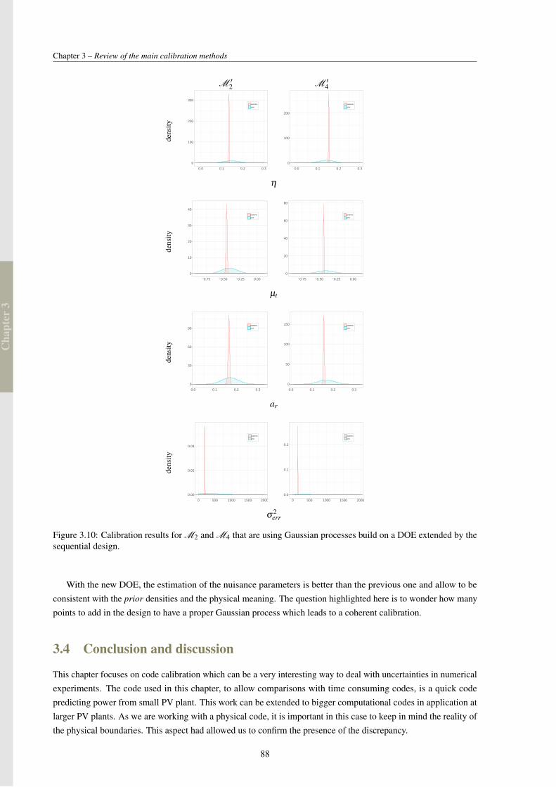
Cha

pter

3

Chapter 3 – Review of the main calibration methods

M ′2 M ′

4

dens

ity0

100

200

300

0.0 0.1 0.2 0.3

posterior

prior

0

100

200

0.0 0.1 0.2 0.3

posterior

prior

η

dens

ity

0

10

20

30

40

−0.75 −0.50 −0.25 0.00

posterior

prior

0

20

40

60

80

−0.75 −0.50 −0.25 0.00

posterior

prior

µt

dens

ity

0

30

60

90

0.0 0.1 0.2 0.3

posterior

prior

0

50

100

150

0.0 0.1 0.2 0.3

posterior

prior

ar

dens

ity

0.00

0.02

0.04

0 500 1000 1500 2000

posterior

prior

0.0

0.1

0.2

0 500 1000 1500 2000

posterior

prior

σ2err

Figure 3.10: Calibration results for M2 and M4 that are using Gaussian processes build on a DOE extended by thesequential design.

With the new DOE, the estimation of the nuisance parameters is better than the previous one and allow to beconsistent with the prior densities and the physical meaning. The question highlighted here is to wonder how manypoints to add in the design to have a proper Gaussian process which leads to a coherent calibration.

3.4 Conclusion and discussion

This chapter focuses on code calibration which can be a very interesting way to deal with uncertainties in numericalexperiments. The code used in this chapter, to allow comparisons with time consuming codes, is a quick codepredicting power from small PV plant. This work can be extended to bigger computational codes in application atlarger PV plants. As we are working with a physical code, it is important in this case to keep in mind the reality ofthe physical boundaries. This aspect had allowed us to confirm the presence of the discrepancy.

88

Cha

pter

3

3.4. Conclusion and discussion

In a case where input variables are correlated, additional issues of DOE appear when the surrogate is fitted. Tocope with these issues we made recourse to a PCA. The design of numerical experiments could have been enhancedby using adaptive designs proposed by Damblin et al. (2018).

The hypotheses made for the application case can also be discussed. For example setting ρ and mδ (.) to 1 and 0is a preliminary decision which goes along with calibration. We do not want to quantify the bias because the aim ofcalibration is to find the parameter value to compensate that bias. If one’s goal is to check where the uncertaintygoes, other hypotheses could have been made. For example, a non zero discrepancy expectation would quantify themean of the gap between the code and the experiments. In calibration we want this gap to be taken into account inthe code through adjusted θ .

The quality of the Gaussian process is also mentioned. Indeed, in code calibration if the estimation of theparameters of the Gaussian process is based on a not satisfactory DOE, calibration quality is then affected. Sometechniques as the sequential design, based of the expected improvement criterion, allow to enhance the initial DOEby finding new points regarding further calibration.

One can wonder which models to use in a given particular case. There is no obvious answer to this questionbut it depends first on the numerical code. If it is time consuming, the first model to try on is M2 and, if it is not,one can use M1. One may then wonder whether it is worth adding a discrepancy term, going from M1 to M3 orfrom M2 to M4. In-depth work on statistical validation had been developed in Damblin et al. (2016) in which thecomparison between two models (with and without discrepancy) is studied in a simplified context. The Bayes factorhelps to decide whether the discrepancy is relevant or not. However, this Bayes factor is burdensome to compute ina general context.

89

Cha

pter

4

CHAPTER4CALICO: A R PACKAGE FOR BAYESIAN

CALIBRATION

4.1 Guidelines for users . . . . . . . . . . . . . . . . . . . . . . . . . . . . . . . . . . . . . . . . . . 92

4.2 Multidimensional example with CaliCo . . . . . . . . . . . . . . . . . . . . . . . . . . . . . . . 97

4.2.1 The models . . . . . . . . . . . . . . . . . . . . . . . . . . . . . . . . . . . . . . . . . . 98

4.2.2 Priors . . . . . . . . . . . . . . . . . . . . . . . . . . . . . . . . . . . . . . . . . . . . . 102

4.2.3 Calibration . . . . . . . . . . . . . . . . . . . . . . . . . . . . . . . . . . . . . . . . . . 103

4.2.4 Additionnal tools . . . . . . . . . . . . . . . . . . . . . . . . . . . . . . . . . . . . . . . 108

4.3 Conclusion . . . . . . . . . . . . . . . . . . . . . . . . . . . . . . . . . . . . . . . . . . . . . . 111

This chapter presents and illustrates the package CaliCo that has been published on CRAN (Comprehensive RArchive Network). It is based on all theoretical developments given Chapter 3. Three packages have been developedfor Bayesian calibration. The package BACCO (Hankin, 2013b) is a bundle of several other packages. It importsemulator (Hankin, 2014), mvtnorm (Genz et al., 2018), calibrator (Hankin, 2013c) and approximator (Hankin,2013a). These packages contain functions that perform Bayesian calibration and also prediction. The statisticalmodel implemented concerns only the case where the numerical code is time consuming and when a code error isadded (the model introduced by Kennedy and O’Hagan (2001)). Moreover, BACCO explores the prior distribution,of the parameters from the statistical model, using analytic or numerical integration. Similarly, another packagecalled SAVE (Palomo et al., 2017) deals with Bayesian calibration through four main functions: SAVE, bayesfit,predictcode and validate. The function SAVE creates the statistical model when bayesfit, predictcode andvalidate perform respectively Bayesian calibration, prediction and validation of a model. Calibration is donein SAVE in a similar way to BACCO because it is based on the same statistical model. Both packages are notflexible with the numerical code and the statistical model. A design of experiments has to be run upstream on thecode before running calibration. The package RobustCalibration based on Gu and Wang (2017) (Gu, 2018b) is apackage that achieves calibration of inexact mathematical models and implements the discrepancy with a “scaledGaussian process”.

CaliCo offers more flexibility on the statistical model choice. If one is interested in calibrating a numericalcode inexpensive in computation time, CaliCo allows the user to upload the numerical code in the model andrun Bayesian calibration with it. A very intuitive perspective is given to the user by using four functions calledmodel, prior, calibrate and forecast, that are detailed in Section 4.1. CaliCo also allows the user to accessseveral ggplot2 (Wickham and Chang, 2016) graphs very easily and to load each of them to change the layoutat one’s convenience. At some point, if the code is time consuming, calibration needs a surrogate to emulate it.Usually, a Gaussian process is chosen (Sacks et al., 1989; Cox et al., 2001). Three packages are related to theestablishment of a Gaussian process as a surrogate: GPfit (MacDoanld et al., 2015), DiceKriging (Roustant et al.,

91

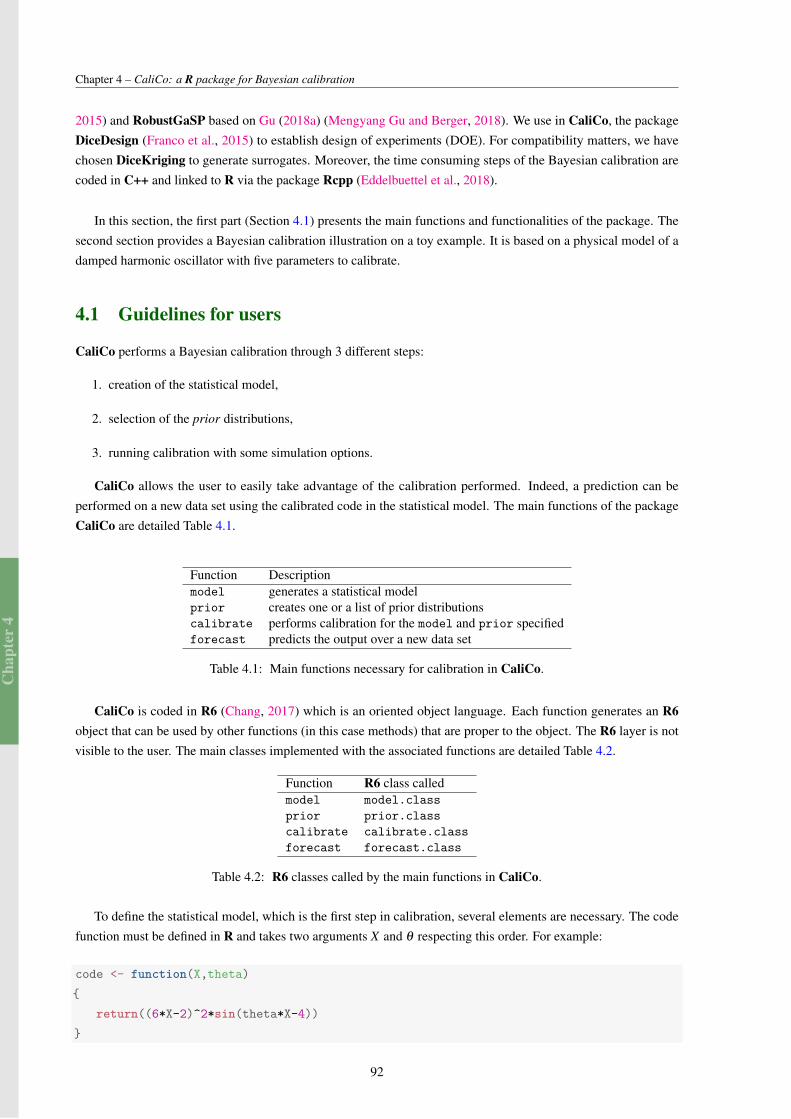
Cha

pter

4

Chapter 4 – CaliCo: a R package for Bayesian calibration

2015) and RobustGaSP based on Gu (2018a) (Mengyang Gu and Berger, 2018). We use in CaliCo, the packageDiceDesign (Franco et al., 2015) to establish design of experiments (DOE). For compatibility matters, we havechosen DiceKriging to generate surrogates. Moreover, the time consuming steps of the Bayesian calibration arecoded in C++ and linked to R via the package Rcpp (Eddelbuettel et al., 2018).

In this section, the first part (Section 4.1) presents the main functions and functionalities of the package. Thesecond section provides a Bayesian calibration illustration on a toy example. It is based on a physical model of adamped harmonic oscillator with five parameters to calibrate.

4.1 Guidelines for users

CaliCo performs a Bayesian calibration through 3 different steps:

1. creation of the statistical model,

2. selection of the prior distributions,

3. running calibration with some simulation options.

CaliCo allows the user to easily take advantage of the calibration performed. Indeed, a prediction can beperformed on a new data set using the calibrated code in the statistical model. The main functions of the packageCaliCo are detailed Table 4.1.

Function Descriptionmodel generates a statistical modelprior creates one or a list of prior distributionscalibrate performs calibration for the model and prior specifiedforecast predicts the output over a new data set

Table 4.1: Main functions necessary for calibration in CaliCo.

CaliCo is coded in R6 (Chang, 2017) which is an oriented object language. Each function generates an R6object that can be used by other functions (in this case methods) that are proper to the object. The R6 layer is notvisible to the user. The main classes implemented with the associated functions are detailed Table 4.2.

Function R6 class calledmodel model.classprior prior.classcalibrate calibrate.classforecast forecast.class

Table 4.2: R6 classes called by the main functions in CaliCo.

To define the statistical model, which is the first step in calibration, several elements are necessary. The codefunction must be defined in R and takes two arguments X and θ respecting this order. For example:

code <- function(X,theta)

return((6*X-2)^2*sin(theta*X-4))

92

Cha

pter

4

4.1. Guidelines for users

If the numerical code is called from another language, one can implement a wrapper that calls from R thenumerical code according to the above writing. It is also possible to build a design of experiments and run the codeoutside R to get the outputs. Then, the DOE and the relative outputs are used instead of the numerical code in thestatistical model (more details below). The function model takes several other arguments (Table 4.3) as for examplethe vector or the matrix of the input variables (described in Section 1.4.1), the vector of experimental data or thestatistical model chosen for calibration.

model description Arguments to be specifiedfc(x,θ) the function to calibrate code (defined as code(x,theta))X the matrix of the input variables Xye the vector of experimental data YexpM the statistical model selected (Default value model1) model1, model2,

model3, model4Gaussian process options (optional only for (Optional) opt.gp (is a list)M2 and M4)Emulation options (optional only for (Optional) opt.emul (is a list)M2 and M4)Simulation options (optional only for (Optional) opt.sim (is a list)M2 and M4)Discrepancy options (necessary only for (Optional) opt.disc (is a list)M3 and M4)

Table 4.3: description of the arguments of the function model.

If the chosen model is M2 or M4, then a Gaussian process will be created as a surrogate of the function code.In each case the Gaussian process option (opt.gp, see Table 4.3) is needed. It is a list which encompasses:

• type: type of covariance function chosen for the surrogate established by the package DiceKriging (Roustantet al., 2015),

• DOE: design of experiments for the surrogate (default value NULL).

Three cases can occur. First, the numerical code is available and the user does not possess any Design OfExperiments (DOE). In this case, only the Gaussian process option opt.gp and the emulation option opt.emul

(Table 4.3) are needed. The emulation option controls the establishment of the DOE. It is a list which contains:

• p: the number of parameters in the model,

• n.emul: the number of points for constituting the DOE,

• binf: the lower bound of the parameter vector,

• bsup: the upper bound of the parameter vector.

The second possible case is when the user want to enforce a specific DOE. Note that in opt.gp, the DOE option isNULL. One can upload a specific DOE in this option. As the new DOE will be used, the emulation option opt.emul

is not needed anymore.

The third case is when no numerical code is available. The user is only in possession of a DOE and thecorresponding code evaluations. Then, the simulation option opt.sim is added. This option encompasses:

• Ysim: the code evaluations of DOEsim,

• DOEsim: the specific DOE used to get simulated data.

93

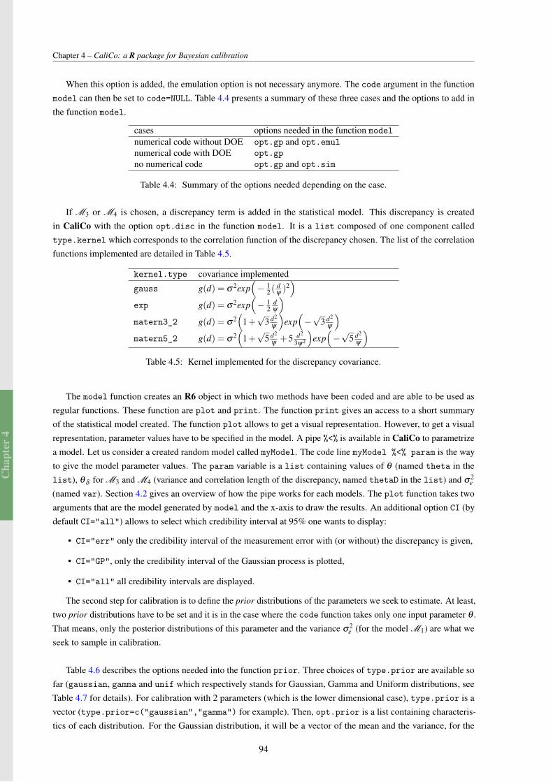
Cha

pter

4

Chapter 4 – CaliCo: a R package for Bayesian calibration

When this option is added, the emulation option is not necessary anymore. The code argument in the functionmodel can then be set to code=NULL. Table 4.4 presents a summary of these three cases and the options to add inthe function model.

cases options needed in the function modelnumerical code without DOE opt.gp and opt.emulnumerical code with DOE opt.gpno numerical code opt.gp and opt.sim

Table 4.4: Summary of the options needed depending on the case.

If M3 or M4 is chosen, a discrepancy term is added in the statistical model. This discrepancy is createdin CaliCo with the option opt.disc in the function model. It is a list composed of one component calledtype.kernel which corresponds to the correlation function of the discrepancy chosen. The list of the correlationfunctions implemented are detailed in Table 4.5.

kernel.type covariance implemented

gauss g(d) = σ2exp(− 1

2 (dψ)2)

exp g(d) = σ2exp(− 1

2dψ

)matern3_2 g(d) = σ2

(1+√

3 d2

ψ

)exp(−√

3 d2

ψ

)matern5_2 g(d) = σ2

(1+√

5 d2

ψ+5 d2

3ψ2

)exp(−√

5 d2

ψ

)Table 4.5: Kernel implemented for the discrepancy covariance.

The model function creates an R6 object in which two methods have been coded and are able to be used asregular functions. These function are plot and print. The function print gives an access to a short summaryof the statistical model created. The function plot allows to get a visual representation. However, to get a visualrepresentation, parameter values have to be specified in the model. A pipe %<% is available in CaliCo to parametrizea model. Let us consider a created random model called myModel. The code line myModel %<% param is the wayto give the model parameter values. The param variable is a list containing values of θ (named theta in thelist), θ δ for M3 and M4 (variance and correlation length of the discrepancy, named thetaD in the list) and σ2

e

(named var). Section 4.2 gives an overview of how the pipe works for each models. The plot function takes twoarguments that are the model generated by model and the x-axis to draw the results. An additional option CI (bydefault CI="all") allows to select which credibility interval at 95% one wants to display:

• CI="err" only the credibility interval of the measurement error with (or without) the discrepancy is given,

• CI="GP", only the credibility interval of the Gaussian process is plotted,

• CI="all" all credibility intervals are displayed.

The second step for calibration is to define the prior distributions of the parameters we seek to estimate. At least,two prior distributions have to be set and it is in the case where the code function takes only one input parameter θ .That means, only the posterior distributions of this parameter and the variance σ2

e (for the model M1) are what weseek to sample in calibration.

Table 4.6 describes the options needed into the function prior. Three choices of type.prior are available sofar (gaussian, gamma and unif which respectively stands for Gaussian, Gamma and Uniform distributions, seeTable 4.7 for details). For calibration with 2 parameters (which is the lower dimensional case), type.prior is avector (type.prior=c("gaussian","gamma") for example). Then, opt.prior is a list containing characteris-tics of each distribution. For the Gaussian distribution, it will be a vector of the mean and the variance, for the

94

Cha

pter

4

4.1. Guidelines for users

prior arguments descriptiontype.prior vector or scalar of string among ("gaussian", "gamma" and "unif")opt.prior list of vector corresponding to the distribution parameters

Table 4.6: description of the arguments of the function prior.

Gamma distribution it will be the shape and the scale and for the Uniform distribution the lower bound and theupper bound (opt.prior=list(c(1,0.1),c(0.01,1)) for example).

type.prior distribution arguments in opt.prior vector

gaussian f (x) = 1√2πV

exp(− 1

2 ((x−m)2

V ))

c(m,V)

gamma f (x) = 1(ka∗Γ(a))x(a−1)exp(− x

k ) c(a,k)unif f (x) = 1

b−a c(a,b)

Table 4.7: description of the arguments of the function prior.

When the prior distributions and the model are defined, calibration can be run. The function calibrate

implements a Markov Chain Monte Carlo (MCMC) according to specific conditions all controlled by the user.

calibrate arguments Descriptionmd the model generated with the function modelpr the list of prior generated by the function prioropt.estim estimation options for calibrationopt.valid (optional) cross validation options (default value NULL)

Table 4.8: description of the arguments of the function calibrate.

The MCMC implemented in CaliCo is composed of two algorithms as described in Section 2.5. The imple-mented algorithm (Algorithm 7) is coded in C++ thanks to Rcpp package (Eddelbuettel et al., 2018) in order tolimit the time consuming aspect of these non-parallelizable loops. Note that there is an adaptability present to reg-ulate the parameter k according to the acceptation rate. The user is free to set that regulation at the wanted percentage.

Then, the opt.estim option is a list composed of:

• Ngibbs: the number of iterations of the Metropolis within Gibbs algorithm,

• Nmh: the number of iteration of the Metropolis Hastings algorithm,

• thetaInit: the starting point,

• r: the vector of regulation of the covariance in the Metropolis within Gibbs algorithm (in the propositiondistribution the variance is kΣ),

• sig: the variance of the proposition distribution Σ,

• Nchains: (default value 1) the number of MCMC chains to run,

• burnIn: the number of iteration to withdraw from the Metropolis Hastings algorithm.

In the function calibrate, one optional argument is available to run a cross validation. This option calledopt.valid, is a list composed of two options which have to be filled:

• type.CV: the type of cross validation wanted (leave one out is the only cross validation implemented so fartype.CV="loo"),

95

Cha

pter

4

Chapter 4 – CaliCo: a R package for Bayesian calibration

• nCV: the number of iteration to run in the cross validation.

After calibration is complete, an R6 object is created and two methods (print and plot) are available and arealso able to be used as regular functions. The print function is a summary that recalls the selected model, thecode used for calibration, the acceptation rate of the Metropolis within Gibbs algorithm, the acceptation rate of theMetropolis Hastings algorithm, the maximum a posteriori and the mean a posteriori. It allows to quickly check theacceptation ratios and see if the chains have properly mixed. The plot function generates automatically, a series ofgraphs that displays, notably, the output of the calibrated code. Two arguments are necessary to run this function:the calibrated model and the x-axis to draw the results. An additional option graph (by default graph="all")allows to control which graphic layout one wants to plot:

• if graph="chains" a layout containing the autocorrelation graphs, the MCMC chains and the prior andposterior distributions for each parameter is given,

• if graph="corr" a layout containing in the diagonal the prior and posterior distributions for the parametervector θ and the scatterplot between each pair of parameters is plotted,

• if graph="results" the result of calibration is displayed,

• if graph="all all of them are printed.

Note that all these graphs (made in ggplot2) are proposed in a particular layout but one can easily load all ofthem into a variable and extract the particular graph one wants. Indeed, if a variable p is used to store all the graphs,then p is a list containing "ACF" (the autocorrelation graphs), "MCMC" (the MCMC chains), "corr" (the scatterplot between each pair of parameters), "dens" (prior and posterior distributions) and "out" (the calibration resultgraph) variables.

Two external functions can be run on an object generated by the function calibrate:

• chain: function that allows to extract the chains sampled in the posterior distribution. If the variableNchains, in opt.estim option, is higher than 1 then the function chain return a coda (Plummer et al.,2016) object with the sampled chains,

• estimators: function that accesses the maximum a posteriori(MAP) and the mean a posteriori.

Sequential design introduced in Damblin et al. (2018) allows to improve the Gaussian process estimation forM2 and M4. Based on the expected improvement (EI), introduced in Jones et al. (1998), new points are added to aninitial DOE in order to improve the quality of calibration. The arguments of the function are given Table 4.9.

sequentialDesign arguments Descriptionmd the model generated with the function model

(for M2 or M4)pr the list of prior generated by the function prioropt.estim estimation options for calibrationk number of points to add in the design

Table 4.9: description of the arguments of the function sequentialDesign.

The last main function in CaliCo is forecast which produces a prediction of a selected model on a new dataand based on previous calibration.

The object generated by forecast.class possesses the two similar methods print and plot. The print

function gives a summary identical to the one in model.class except that it adds the MAP estimator. The plot

96

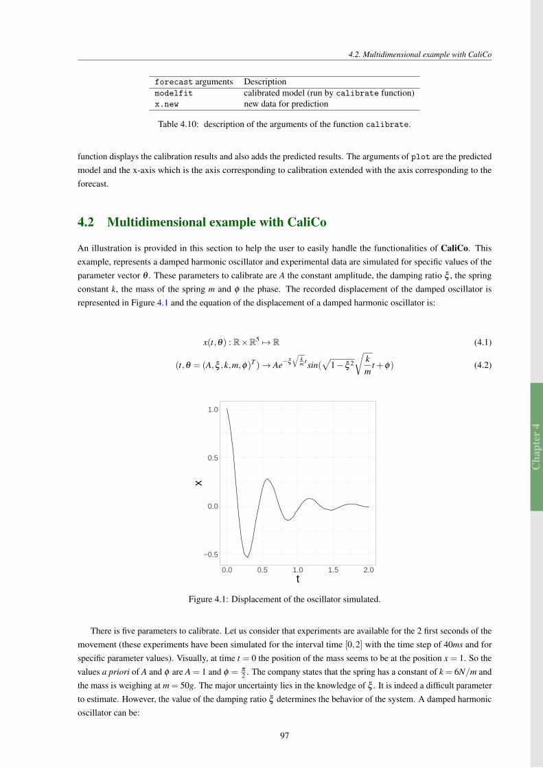
Cha

pter

4

4.2. Multidimensional example with CaliCo

forecast arguments Descriptionmodelfit calibrated model (run by calibrate function)x.new new data for prediction

Table 4.10: description of the arguments of the function calibrate.

function displays the calibration results and also adds the predicted results. The arguments of plot are the predictedmodel and the x-axis which is the axis corresponding to calibration extended with the axis corresponding to theforecast.

4.2 Multidimensional example with CaliCo

An illustration is provided in this section to help the user to easily handle the functionalities of CaliCo. Thisexample, represents a damped harmonic oscillator and experimental data are simulated for specific values of theparameter vector θ . These parameters to calibrate are A the constant amplitude, the damping ratio ξ , the springconstant k, the mass of the spring m and φ the phase. The recorded displacement of the damped oscillator isrepresented in Figure 4.1 and the equation of the displacement of a damped harmonic oscillator is:

x(t,θ) : R×R5 7→ R (4.1)

(t,θ = (A,ξ ,k,m,φ)T )→ Ae−ξ

√km tsin(

√1−ξ 2

√km

t +φ) (4.2)

−0.5

0.0

0.5

1.0

0.0 0.5 1.0 1.5 2.0t

x

Figure 4.1: Displacement of the oscillator simulated.

There is five parameters to calibrate. Let us consider that experiments are available for the 2 first seconds of themovement (these experiments have been simulated for the interval time [0,2] with the time step of 40ms and forspecific parameter values). Visually, at time t = 0 the position of the mass seems to be at the position x = 1. So thevalues a priori of A and φ are A = 1 and φ = π

2 . The company states that the spring has a constant of k = 6N/m andthe mass is weighing at m = 50g. The major uncertainty lies in the knowledge of ξ . It is indeed a difficult parameterto estimate. However, the value of the damping ratio ξ determines the behavior of the system. A damped harmonicoscillator can be:

97

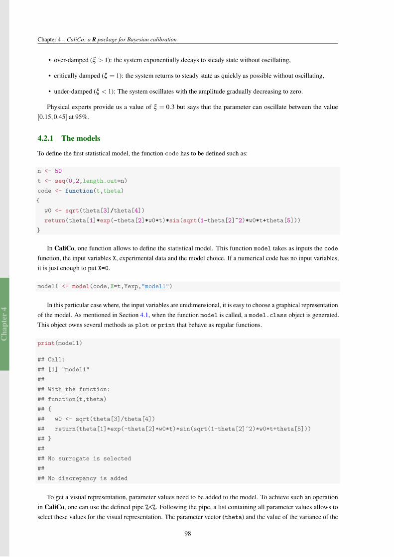
Cha

pter

4

Chapter 4 – CaliCo: a R package for Bayesian calibration

• over-damped (ξ > 1): the system exponentially decays to steady state without oscillating,

• critically damped (ξ = 1): the system returns to steady state as quickly as possible without oscillating,

• under-damped (ξ < 1): The system oscillates with the amplitude gradually decreasing to zero.

Physical experts provide us a value of ξ = 0.3 but says that the parameter can oscillate between the value[0.15,0.45] at 95%.

4.2.1 The models

To define the first statistical model, the function code has to be defined such as:

n <- 50

t <- seq(0,2,length.out=n)

code <- function(t,theta)

w0 <- sqrt(theta[3]/theta[4])

return(theta[1]*exp(-theta[2]*w0*t)*sin(sqrt(1-theta[2]^2)*w0*t+theta[5]))

In CaliCo, one function allows to define the statistical model. This function model takes as inputs the code

function, the input variables X, experimental data and the model choice. If a numerical code has no input variables,it is just enough to put X=0.

model1 <- model(code,X=t,Yexp,"model1")

In this particular case where, the input variables are unidimensional, it is easy to choose a graphical representationof the model. As mentioned in Section 4.1, when the function model is called, a model.class object is generated.This object owns several methods as plot or print that behave as regular functions.

print(model1)

## Call:

## [1] "model1"

##

## With the function:

## function(t,theta)

##

## w0 <- sqrt(theta[3]/theta[4])

## return(theta[1]*exp(-theta[2]*w0*t)*sin(sqrt(1-theta[2]^2)*w0*t+theta[5]))

##

##

## No surrogate is selected

##

## No discrepancy is added

To get a visual representation, parameter values need to be added to the model. To achieve such an operationin CaliCo, one can use the defined pipe %<%. Following the pipe, a list containing all parameter values allows toselect these values for the visual representation. The parameter vector (theta) and the value of the variance of the

98

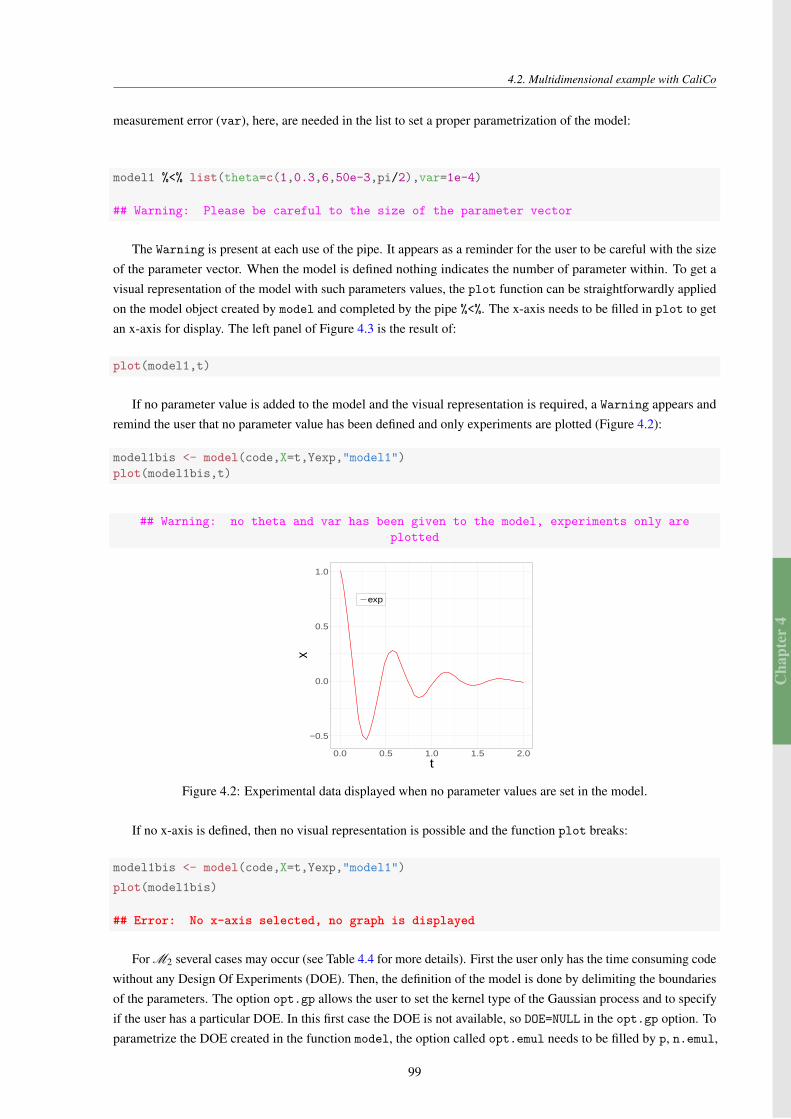
Cha

pter

4

4.2. Multidimensional example with CaliCo

measurement error (var), here, are needed in the list to set a proper parametrization of the model:

model1 %<% list(theta=c(1,0.3,6,50e-3,pi/2),var=1e-4)

## Warning: Please be careful to the size of the parameter vector

The Warning is present at each use of the pipe. It appears as a reminder for the user to be careful with the sizeof the parameter vector. When the model is defined nothing indicates the number of parameter within. To get avisual representation of the model with such parameters values, the plot function can be straightforwardly appliedon the model object created by model and completed by the pipe %<%. The x-axis needs to be filled in plot to getan x-axis for display. The left panel of Figure 4.3 is the result of:

plot(model1,t)

If no parameter value is added to the model and the visual representation is required, a Warning appears andremind the user that no parameter value has been defined and only experiments are plotted (Figure 4.2):

model1bis <- model(code,X=t,Yexp,"model1")plot(model1bis,t)

## Warning: no theta and var has been given to the model, experiments only areplotted

−0.5

0.0

0.5

1.0

0.0 0.5 1.0 1.5 2.0t

x

exp

Figure 4.2: Experimental data displayed when no parameter values are set in the model.

If no x-axis is defined, then no visual representation is possible and the function plot breaks:

model1bis <- model(code,X=t,Yexp,"model1")

plot(model1bis)

## Error: No x-axis selected, no graph is displayed

For M2 several cases may occur (see Table 4.4 for more details). First the user only has the time consuming codewithout any Design Of Experiments (DOE). Then, the definition of the model is done by delimiting the boundariesof the parameters. The option opt.gp allows the user to set the kernel type of the Gaussian process and to specifyif the user has a particular DOE. In this first case the DOE is not available, so DOE=NULL in the opt.gp option. Toparametrize the DOE created in the function model, the option called opt.emul needs to be filled by p, n.emul,

99

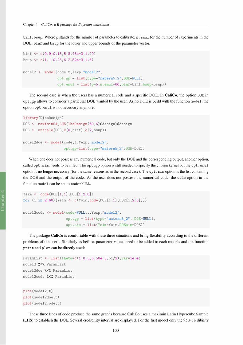
Cha

pter

4

Chapter 4 – CaliCo: a R package for Bayesian calibration

binf, bsup. Where p stands for the number of parameter to calibrate, n.emul for the number of experiments in theDOE, binf and bsup for the lower and upper bounds of the parameter vector.

binf <- c(0.9,0.15,5.8,48e-3,1.49)

bsup <- c(1.1,0.45,6.2,52e-3,1.6)

model2 <- model(code,t,Yexp,"model2",

opt.gp = list(type="matern5_2",DOE=NULL),

opt.emul = list(p=5,n.emul=60,binf=binf,bsup=bsup))

The second case is when the users has a numerical code and a specific DOE. In CaliCo, the option DOE inopt.gp allows to consider a particular DOE wanted by the user. As no DOE is build with the function model, theoption opt.emul is not necessary anymore:

library(DiceDesign)

DOE <- maximinSA_LHS(lhsDesign(60,6)$design)$design

DOE <- unscale(DOE,c(0,binf),c(2,bsup))

model2doe <- model(code,t,Yexp,"model2",

opt.gp=list(type="matern5_2",DOE=DOE))

When one does not possess any numerical code, but only the DOE and the corresponding output, another option,called opt.sim, needs to be filled. The opt.gp option is still needed to specify the chosen kernel but the opt.emul

option is no longer necessary (for the same reasons as in the second case). The opt.sim option is the list containingthe DOE and the output of the code. As the user does not possess the numerical code, the code option in thefunction model can be set to code=NULL.

Ysim <- code(DOE[1,1],DOE[1,2:6])

for (i in 2:60)Ysim <- c(Ysim,code(DOE[i,1],DOE[i,2:6]))

model2code <- model(code=NULL,t,Yexp,"model2",

opt.gp = list(type="matern5_2", DOE=NULL),

opt.sim = list(Ysim=Ysim,DOEsim=DOE))

The package CaliCo is comfortable with these three situations and bring flexibility according to the differentproblems of the users. Similarly as before, parameter values need to be added to each models and the functionprint and plot can be directly used:

ParamList <- list(theta=c(1,0.3,6,50e-3,pi/2),var=1e-4)

model2 %<% ParamList

model2doe %<% ParamList

model2code %<% ParamList

plot(model2,t)

plot(model2doe,t)

plot(model2code,t)

These three lines of code produce the same graphs because CaliCo uses a maximin Latin Hypercube Sample(LHS) to establish the DOE. Several credibility interval are displayed. For the first model only the 95% credibility

100

Cha

pter

4

4.2. Multidimensional example with CaliCo

interval of the measurement error is available. For the second model, the 95% credibility interval of the Gaussianprocess can also be shown. Figure 4.3 illustrates M1 and M2.

M1 M2

−0.5

0.0

0.5

1.0

0.0 0.5 1.0 1.5 2.0t

x

CI 95% noise

expmodel output

−0.5

0.0

0.5

1.0

0.0 0.5 1.0 1.5 2.0t

x

expmodel output

CI 95% GPCI 95% noise

Figure 4.3: First and second model output for prior belief on parameter values. The left panel illustrates the firstmodel and the right panel the second model with the Gaussian process estimated.

One can be interested in modeling a code discrepancy. When the code is not time consuming, the model tochoose is M3. The opt.disc option allows to specify the kernel type of the discrepancy. Note that the visualrepresentation requires initial values for the discrepancy and are needed in the pipe %<%. This vector thetaD iscomposed of σ2 and ψ according to Table 4.5.

model3 <- model(code,t,Yexp,"model3",

opt.disc = list(kernel.type="gauss"))

model3 %<% list(theta=c(1,0.3,6,50e-3,pi/2),thetaD=c(1e-4,0.2),var=1e-4)

When the code is time consuming, then M4 is selected. The same cases can occur as for M2 but only the casewhere the code is not available will be considered, here, for M4.

model4 <- model(code=NULL,t,Yexp,"model4",

opt.gp = list(type="matern5_2", DOE=NULL),

opt.sim = list(Ysim=Ysim,DOEsim=DOE),

opt.disc = list(kernel.type="gauss"))

model4 %<% list(theta=c(1,0.3,6,50e-3,pi/2),thetaD=c(1e-4,0.2),var=1e-4)

To get a visual representation of M3 and M4, the function plot is defined identically as before. The results aredisplayed in Figure 4.4.

plot(model3,t)

plot(model4,t)

Note that several credibility intervals can be displayed. By default all of them are shown (for example see rightpanels of Figure 4.3 and Figure 4.4). For M1 and M3 only one credibility interval is given. It represents the 95%credibility interval of the measurement error, in the case of M1, and the 95% credibility interval of the measurementerror plus the discrepancy, in the case of M3. For M2 and M4, two credibility intervals are available. Compared toM1 and M3 the credibility interval at 95% of the Gaussian process, that emulates the code, is added. It allows to

101

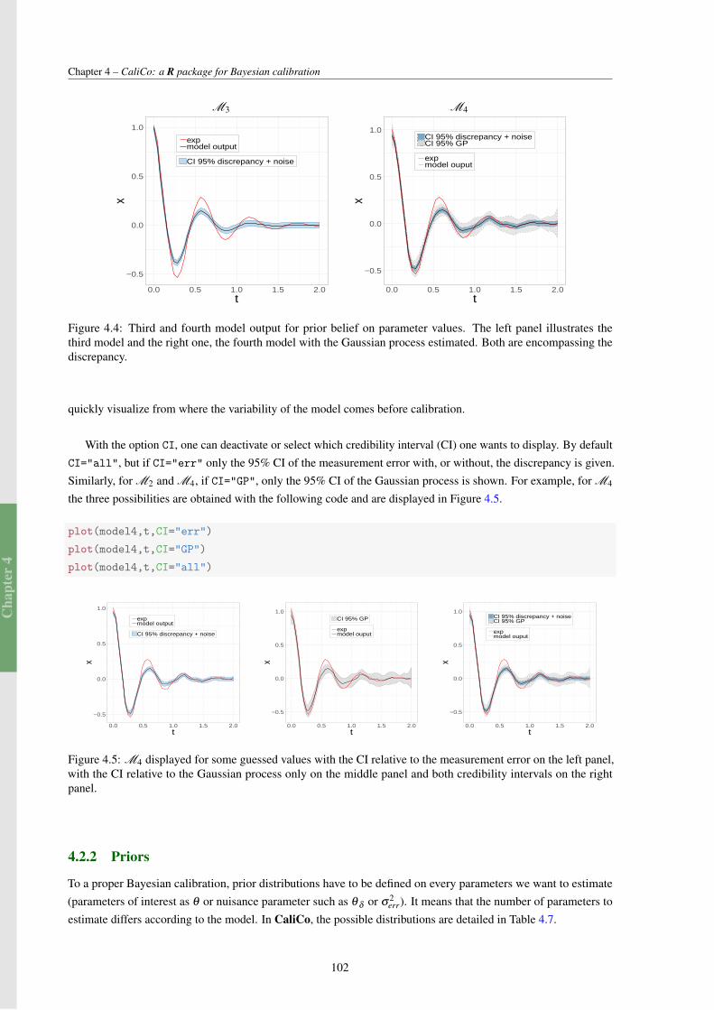
Cha

pter

4

Chapter 4 – CaliCo: a R package for Bayesian calibration

M3 M4

−0.5

0.0

0.5

1.0

0.0 0.5 1.0 1.5 2.0t

x

expmodel output

CI 95% discrepancy + noise

−0.5

0.0

0.5

1.0

0.0 0.5 1.0 1.5 2.0t

x

CI 95% discrepancy + noiseCI 95% GP

expmodel ouput

Figure 4.4: Third and fourth model output for prior belief on parameter values. The left panel illustrates thethird model and the right one, the fourth model with the Gaussian process estimated. Both are encompassing thediscrepancy.

quickly visualize from where the variability of the model comes before calibration.

With the option CI, one can deactivate or select which credibility interval (CI) one wants to display. By defaultCI="all", but if CI="err" only the 95% CI of the measurement error with, or without, the discrepancy is given.Similarly, for M2 and M4, if CI="GP", only the 95% CI of the Gaussian process is shown. For example, for M4

the three possibilities are obtained with the following code and are displayed in Figure 4.5.

plot(model4,t,CI="err")

plot(model4,t,CI="GP")

plot(model4,t,CI="all")

−0.5

0.0

0.5

1.0

0.0 0.5 1.0 1.5 2.0t

x

expmodel output

CI 95% discrepancy + noise

−0.5

0.0

0.5

1.0

0.0 0.5 1.0 1.5 2.0t

x

CI 95% GP

expmodel ouput

−0.5

0.0

0.5

1.0

0.0 0.5 1.0 1.5 2.0t

x

CI 95% discrepancy + noiseCI 95% GP

expmodel ouput

Figure 4.5: M4 displayed for some guessed values with the CI relative to the measurement error on the left panel,with the CI relative to the Gaussian process only on the middle panel and both credibility intervals on the rightpanel.

4.2.2 Priors

To a proper Bayesian calibration, prior distributions have to be defined on every parameters we want to estimate(parameters of interest as θ or nuisance parameter such as θ δ or σ2

err). It means that the number of parameters toestimate differs according to the model. In CaliCo, the possible distributions are detailed in Table 4.7.

102

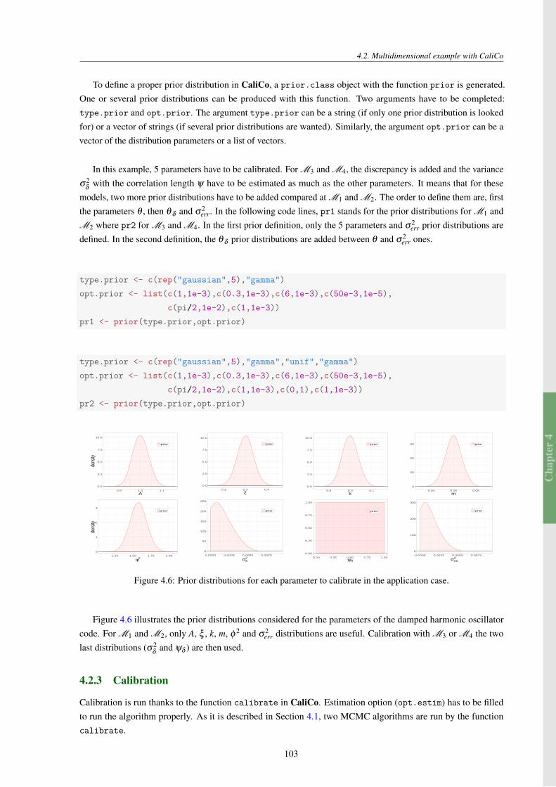
Cha

pter

4

4.2. Multidimensional example with CaliCo

To define a proper prior distribution in CaliCo, a prior.class object with the function prior is generated.One or several prior distributions can be produced with this function. Two arguments have to be completed:type.prior and opt.prior. The argument type.prior can be a string (if only one prior distribution is lookedfor) or a vector of strings (if several prior distributions are wanted). Similarly, the argument opt.prior can be avector of the distribution parameters or a list of vectors.

In this example, 5 parameters have to be calibrated. For M3 and M4, the discrepancy is added and the varianceσ2

δwith the correlation length ψ have to be estimated as much as the other parameters. It means that for these

models, two more prior distributions have to be added compared at M1 and M2. The order to define them are, firstthe parameters θ , then θ δ and σ2

err. In the following code lines, pr1 stands for the prior distributions for M1 andM2 where pr2 for M3 and M4. In the first prior definition, only the 5 parameters and σ2

err prior distributions aredefined. In the second definition, the θ δ prior distributions are added between θ and σ2

err ones.

type.prior <- c(rep("gaussian",5),"gamma")

opt.prior <- list(c(1,1e-3),c(0.3,1e-3),c(6,1e-3),c(50e-3,1e-5),

c(pi/2,1e-2),c(1,1e-3))

pr1 <- prior(type.prior,opt.prior)

type.prior <- c(rep("gaussian",5),"gamma","unif","gamma")

opt.prior <- list(c(1,1e-3),c(0.3,1e-3),c(6,1e-3),c(50e-3,1e-5),

c(pi/2,1e-2),c(1,1e-3),c(0,1),c(1,1e-3))

pr2 <- prior(type.prior,opt.prior)

0.0

2.5

5.0

7.5

10.0

0.9 1.0 1.1A

dens

ity

prior

0.0

2.5

5.0

7.5

10.0

0.2 0.3 0.4ξ

prior

0.0

2.5

5.0

7.5

10.0

5.9 6.0 6.1k

prior

0

30

60

90

0.04 0.05 0.06m

prior

0

1

2

3

1.25 1.50 1.75 2.00

φ2

dens

ity

prior

0

50

100

150

200

250

0.0000 0.0025 0.0050 0.0075

σδ2

prior

0.00

0.25

0.50

0.75

1.00

0.00 0.25 0.50 0.75 1.00ψδ

prior

0

100

200

300

0.0000 0.0025 0.0050 0.0075

σerr2

prior

Figure 4.6: Prior distributions for each parameter to calibrate in the application case.

Figure 4.6 illustrates the prior distributions considered for the parameters of the damped harmonic oscillatorcode. For M1 and M2, only A, ξ , k, m, φ 2 and σ2

err distributions are useful. Calibration with M3 or M4 the twolast distributions (σ2

δand ψδ ) are then used.

4.2.3 Calibration

Calibration is run thanks to the function calibrate in CaliCo. Estimation option (opt.estim) has to be filledto run the algorithm properly. As it is described in Section 4.1, two MCMC algorithms are run by the functioncalibrate.

103

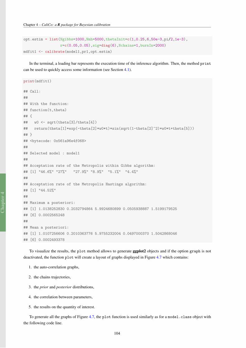
Cha

pter

4

Chapter 4 – CaliCo: a R package for Bayesian calibration

opt.estim = list(Ngibbs=1000,Nmh=5000,thetaInit=c(1,0.25,6,50e-3,pi/2,1e-3),

r=c(0.05,0.05),sig=diag(6),Nchains=1,burnIn=2000)

mdfit1 <- calibrate(model1,pr1,opt.estim)

In the terminal, a loading bar represents the execution time of the inference algorithm. Then, the method print

can be used to quickly access some information (see Section 4.1).

print(mdfit1)

## Call:

##

## With the function:

## function(t,theta)

##

## w0 <- sqrt(theta[3]/theta[4])

## return(theta[1]*exp(-theta[2]*w0*t)*sin(sqrt(1-theta[2]^2)*w0*t+theta[5]))

##

## <bytecode: 0x561a96e4f068>

##

## Selected model : model1

##

## Acceptation rate of the Metropolis within Gibbs algorithm:

## [1] "46.6%" "27%" "27.9%" "8.9%" "5.1%" "4.4%"

##

## Acceptation rate of the Metropolis Hastings algorithm:

## [1] "44.52%"

##

## Maximum a posteriori:

## [1] 1.0138252830 0.2032794864 5.9924680899 0.0505938887 1.5199179525

## [6] 0.0002565248

##

## Mean a posteriori:

## [1] 1.0107256606 0.2010363776 5.9755232004 0.0497000370 1.5042868046

## [6] 0.0002493378

To visualize the results, the plot method allows to generate ggplot2 objects and if the option graph is notdeactivated, the function plot will create a layout of graphs displayed in Figure 4.7 which contains:

1. the auto-correlation graphs,

2. the chains trajectories,

3. the prior and posterior distributions,

4. the correlation between parameters,

5. the results on the quantity of interest.

To generate all the graphs of Figure 4.7, the plot function is used similarly as for a model.class object withthe following code line.

104

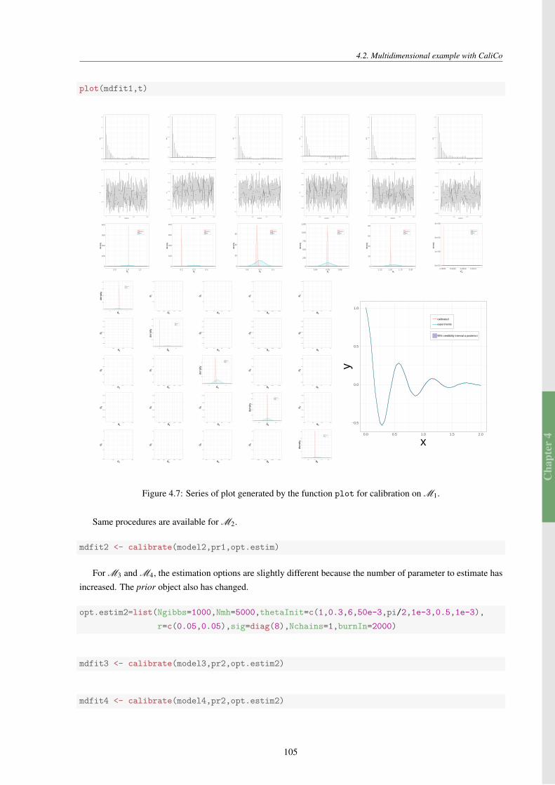
Cha

pter

4

4.2. Multidimensional example with CaliCo

plot(mdfit1,t)

0.00

0.25

0.50

0.75

1.00

0 10 20 30

Lag

AC

F

0.00

0.25

0.50

0.75

1.00

0 10 20 30

LagA

CF

0.00

0.25

0.50

0.75

1.00

0 10 20 30

Lag

AC

F

0.00

0.25

0.50

0.75

1.00

0 10 20 30

Lag

AC

F

0.00

0.25

0.50

0.75

1.00

0 10 20 30

Lag

AC

F

0.00

0.25

0.50

0.75

1.00

0 10 20 30

Lag

AC

F

1.010

1.012

1.014

0 1000 2000 3000

iterations

θ 1

0.199

0.200

0.201

0.202

0.203

0 1000 2000 3000

iterations

θ 2

5.96

5.97

5.98

5.99

0 1000 2000 3000

iterations

θ 3

0.0490

0.0495

0.0500

0.0505

0 1000 2000 3000

iterations

θ 4

1.49

1.50

1.51

1.52

0 1000 2000 3000

iterations

θ 5

0.000244

0.000248

0.000252

0.000256

0 1000 2000 3000

iterations

σ err

2

0

100

200

300

400

0.9 1.0 1.1θ1

dens

ity

posterior

prior

0

100

200

300

400

0.2 0.3 0.4θ2

dens

ity

posterior

prior

0

20

40

60

5.9 6.0 6.1θ3

dens

ityposterior

prior

0

250

500

750

1000

1250

0.04 0.05 0.06θ4

dens

ity

posterior

prior

0

20

40

60

80

1.25 1.50 1.75 2.00θ5

dens

ity

posterior

prior

0e+00

1e+05

2e+05

3e+05

0.0000 0.0025 0.0050 0.0075σerr

2

dens

ity

posterior

prior

0

100

200

300

400

0.9 1.0 1.1

θ1

dens

ity

posterior

prior

1.010

1.012

1.014

0.199 0.200 0.201 0.202 0.203

θ2

θ 1

1.010

1.012

1.014

5.96 5.97 5.98 5.99

θ3

θ 1

1.010

1.012

1.014

0.0490 0.0495 0.0500 0.0505

θ4

θ 1

1.010

1.012

1.014

1.49 1.50 1.51 1.52

θ5

θ 1

0.199

0.200

0.201

0.202

0.203

1.010 1.012 1.014

θ1

θ 2

0

100

200

300

400

0.2 0.3 0.4

θ2

dens

ity

posterior

prior

0.199

0.200

0.201

0.202

0.203

5.96 5.97 5.98 5.99

θ3

θ 2

0.199

0.200

0.201

0.202

0.203

0.0490 0.0495 0.0500 0.0505

θ4

θ 2

0.199

0.200

0.201

0.202

0.203

1.49 1.50 1.51 1.52

θ5

θ 2

5.96

5.97

5.98

5.99

1.010 1.012 1.014

θ1

θ 3

5.96

5.97

5.98

5.99

0.199 0.200 0.201 0.202 0.203

θ2

θ 3

0

20

40

60

5.9 6.0 6.1

θ3

dens

ity

posterior

prior

5.96

5.97

5.98

5.99

0.0490 0.0495 0.0500 0.0505

θ4

θ 3

5.96

5.97

5.98

5.99

1.49 1.50 1.51 1.52

θ5

θ 3

0.0490

0.0495

0.0500

0.0505

1.010 1.012 1.014

θ1

θ 4

0.0490

0.0495

0.0500

0.0505

0.199 0.200 0.201 0.202 0.203

θ2

θ 4

0.0490

0.0495

0.0500

0.0505

5.96 5.97 5.98 5.99

θ3

θ 4

0

250

500

750

1000

1250

0.04 0.05 0.06

θ4

dens

ity

posterior

prior

0.0490

0.0495

0.0500

0.0505

1.49 1.50 1.51 1.52

θ5

θ 4

1.49

1.50

1.51

1.52

1.010 1.012 1.014

θ1

θ 5

1.49

1.50

1.51

1.52

0.199 0.200 0.201 0.202 0.203

θ2

θ 5

1.49

1.50

1.51

1.52

5.96 5.97 5.98 5.99

θ3

θ 5

1.49

1.50

1.51

1.52

0.0490 0.0495 0.0500 0.0505

θ4

θ 5

0

20

40

60

80

1.25 1.50 1.75 2.00

θ5

dens

ity

posterior

prior

−0.5

0.0

0.5

1.0

0.0 0.5 1.0 1.5 2.0

x

y

calibrated

experiments

95% credibility interval a posteriori

Figure 4.7: Series of plot generated by the function plot for calibration on M1.

Same procedures are available for M2.

mdfit2 <- calibrate(model2,pr1,opt.estim)

For M3 and M4, the estimation options are slightly different because the number of parameter to estimate hasincreased. The prior object also has changed.

opt.estim2=list(Ngibbs=1000,Nmh=5000,thetaInit=c(1,0.3,6,50e-3,pi/2,1e-3,0.5,1e-3),

r=c(0.05,0.05),sig=diag(8),Nchains=1,burnIn=2000)

mdfit3 <- calibrate(model3,pr2,opt.estim2)

mdfit4 <- calibrate(model4,pr2,opt.estim2)

105

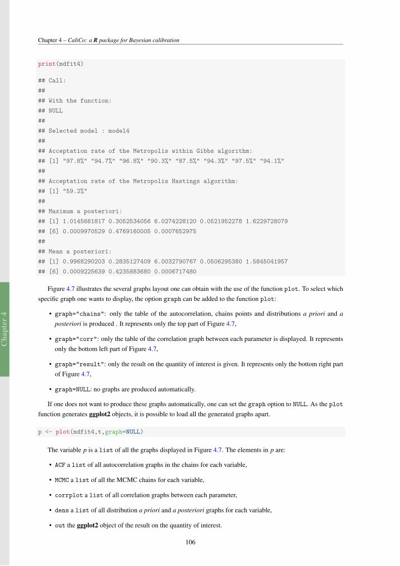
Cha

pter

4

Chapter 4 – CaliCo: a R package for Bayesian calibration

print(mdfit4)

## Call:

##

## With the function:

## NULL

##

## Selected model : model4

##

## Acceptation rate of the Metropolis within Gibbs algorithm:

## [1] "97.8%" "94.7%" "96.8%" "90.3%" "87.5%" "94.3%" "97.5%" "94.1%"

##

## Acceptation rate of the Metropolis Hastings algorithm:

## [1] "59.2%"

##

## Maximum a posteriori:

## [1] 1.0145661817 0.3052534056 6.0274228120 0.0521952278 1.6229728079

## [6] 0.0009970529 0.4769160005 0.0007652975

##

## Mean a posteriori:

## [1] 0.9968290203 0.2835127409 6.0032790767 0.0506295380 1.5845041957

## [6] 0.0009225639 0.4235883680 0.0006717480

Figure 4.7 illustrates the several graphs layout one can obtain with the use of the function plot. To select whichspecific graph one wants to display, the option graph can be added to the function plot:

• graph="chains": only the table of the autocorrelation, chains points and distributions a priori and a

posteriori is produced . It represents only the top part of Figure 4.7,

• graph="corr": only the table of the correlation graph between each parameter is displayed. It representsonly the bottom left part of Figure 4.7,

• graph="result": only the result on the quantity of interest is given. It represents only the bottom right partof Figure 4.7,

• graph=NULL: no graphs are produced automatically.

If one does not want to produce these graphs automatically, one can set the graph option to NULL. As the plot

function generates ggplot2 objects, it is possible to load all the generated graphs apart.

p <- plot(mdfit4,t,graph=NULL)

The variable p is a list of all the graphs displayed in Figure 4.7. The elements in p are:

• ACF a list of all autocorrelation graphs in the chains for each variable,

• MCMC a list of all the MCMC chains for each variable,

• corrplot a list of all correlation graphs between each parameter,

• dens a list of all distribution a priori and a posteriori graphs for each variable,

• out the ggplot2 object of the result on the quantity of interest.

106

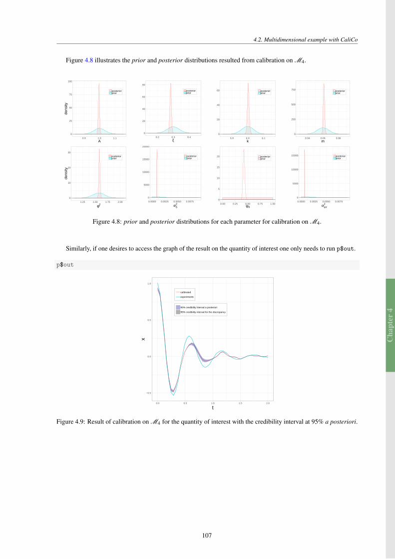
Cha

pter

4

4.2. Multidimensional example with CaliCo

Figure 4.8 illustrates the prior and posterior distributions resulted from calibration on M4.

0

25

50

75

100

0.9 1.0 1.1A

dens

ity

posteriorprior

0

20

40

60

80

0.2 0.3 0.4ξ

posteriorprior

0

20

40

60

5.9 6.0 6.1k

posteriorprior

0

250

500

750

0.04 0.05 0.06m

posteriorprior

0

10

20

30

1.25 1.50 1.75 2.00

φ2

dens

ity

posteriorprior

0

5000

10000

15000

20000

0.0000 0.0025 0.0050 0.0075

σδ2

posteriorprior

0

5

10

15

20

0.00 0.25 0.50 0.75 1.00ψδ

posteriorprior

0

5000

10000

15000

0.0000 0.0025 0.0050 0.0075

σerr2

posteriorprior

Figure 4.8: prior and posterior distributions for each parameter for calibration on M4.

Similarly, if one desires to access the graph of the result on the quantity of interest one only needs to run p$out.

p$out

−0.5

0.0

0.5

1.0

0.0 0.5 1.0 1.5 2.0

t

x

calibrated

experiments

95% credibility interval a posteriori

95% credibility interval for the discrepancy

Figure 4.9: Result of calibration on M4 for the quantity of interest with the credibility interval at 95% a posteriori.

107

Cha

pter

4

Chapter 4 – CaliCo: a R package for Bayesian calibration

4.2.4 Additionnal tools

A function in CaliCo called estimators allows to access estimators as the MAP and the mean a posteriori.

estimators(mdfit1)

## $MAP

## [1] 1.0105967765 0.2011318973 5.9741254796 0.0496559638 1.5042583733

## [6] 0.0002488385

##

## $MEAN

## [1] 1.0107256606 0.2010363776 5.9755232004 0.0497000370 1.5042868046

## [6] 0.0002493378

If one is interested in running convergence diagnostics on the MCMC chains run by the function calibrate,one is free to increase the number of chains in the opt.estim options. This operation is accomplished in parallelwith an automatically detected number of cores.

opt.estim=list(Ngibbs=1000,Nmh=5000,thetaInit=c(1,0.25,6,50e-3,pi/2,1e-3),

r=c(0.05,0.05),sig=diag(6),Nchains=3,burnIn=2000)

mdfitMCMC <- calibrate(model1,pr1,opt.estim)

By setting Nchains=3, calibration is run 3 times. The function chain allows to load the coda object generatedand then to use coda tools as Gelman-Rubin diagnostics (Gelman and Rubin, 1992) for example.

mcmc <- chain(mdfitMCMC)

library(coda)

gelman.diag(mcmc)

## Potential scale reduction factors:

##

## Point est. Upper C.I.

## [1,] 4.00 7.81

## [2,] 1.55 2.39

## [3,] 8.58 16.65

## [4,] 1.25 1.68

## [5,] 3.52 7.23

## [6,] 38.66 75.48

##

## Multivariate psrf

##

## 31.3

The user can also run very easily a cross validation (a leave one out) to estimate how accurately the modelprediction will perform in practice. An additional option, called opt.valid, is then necessary to run this crossvalidation. This option is a list containing the number of iteration (nCV) and the type cross validation method(type.valid).

108

Cha

pter

4

4.2. Multidimensional example with CaliCo

mdfitCV <- calibrate(model1,pr1,

opt.estim = list(Ngibbs=1000,

Nmh=5000,

thetaInit=c(1,0.25,6,50e-3,pi/2,1e-3),

r=c(0.05,0.05),

sig=diag(6),

Nchains=1,

burnIn=2000),

opt.valid = list(type.valid="loo",

nCV=50))

The activation of the cross validation will run the regular calibration and then the nCV iterations requested by theuser. To decrease the computational burden of such operation, a parallel operation is performed by to the packageparallel present in R core.

print(mdfitCV)

## Call:

##

## With the function:

## function(t,theta)

##

## w0 <- sqrt(theta[3]/theta[4])

## return(theta[1]*exp(-theta[2]*w0*t)*sin(sqrt(1-theta[2]^2)*w0*t+theta[5]))

##

## <bytecode: 0x561a93b33348>

##

## Selected model : model1

##

## Acceptation rate of the Metropolis within Gibbs algorithm:

## [1] "43.8%" "27.5%" "27.3%" "9.1%" "4.3%" "4.4%"

##

## Acceptation rate of the Metropolis Hastings algorithm:

## [1] "48.56%"

##

## Maximum a posteriori:

## [1] 1.0144067620 0.2032408379 6.0077799738 0.0508023686 1.5169972084

## [6] 0.0002536493

##

## Mean a posteriori:

## [1] 1.0121094549 0.2016018588 5.9975259667 0.0499179223 1.5060238122

## [6] 0.0002488799

##

##

## Cross validation:

## Method: loo

## Predicted Real Error

## 1 0.581834516 0.58394961 0.0021150930

109

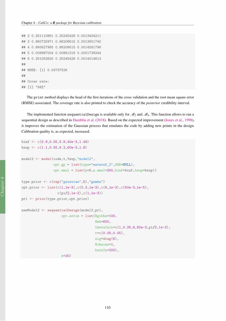
Cha

pter

4

Chapter 4 – CaliCo: a R package for Bayesian calibration

## 2 0.251110861 0.25245428 0.0013434211

## 3 0.860725971 0.86208615 0.0013601740

## 4 0.860627965 0.86208615 0.0014581796

## 5 0.009987004 0.00981318 0.0001738244

## 6 0.251052820 0.25245428 0.0014014613

##

## RMSE: [1] 0.03737526

##

## Cover rate:

## [1] "94%"

The print method displays the head of the first iterations of the cross validation and the root mean square error(RMSE) associated. The coverage rate is also printed to check the accuracy of the posterior credibility interval.

The implemented function sequentialDesign is available only for M2 and M4. This function allows to run asequential design as described in Damblin et al. (2018). Based on the expected improvement (Jones et al., 1998),it improves the estimation of the Gaussian process that emulates the code by adding new points in the design.Calibration quality is, as expected, increased.

binf <- c(0.9,0.05,5.8,40e-3,1.49)

bsup <- c(1.1,0.55,6.2,60e-3,1.6)

model2 <- model(code,t,Yexp,"model2",

opt.gp = list(type="matern5_2",DOE=NULL),

opt.emul = list(p=5,n.emul=200,binf=binf,bsup=bsup))

type.prior <- c(rep("gaussian",5),"gamma")

opt.prior <- list(c(1,1e-3),c(0.3,1e-3),c(6,1e-3),c(50e-3,1e-5),

c(pi/2,1e-2),c(1,1e-3))

pr1 <- prior(type.prior,opt.prior)

newModel2 <- sequentialDesign(model2,pr1,

opt.estim = list(Ngibbs=100,

Nmh=600,

thetaInit=c(1,0.25,6,50e-3,pi/2,1e-3),

r=c(0.05,0.05),

sig=diag(6),

Nchains=1,

burnIn=200),

k=20)

110

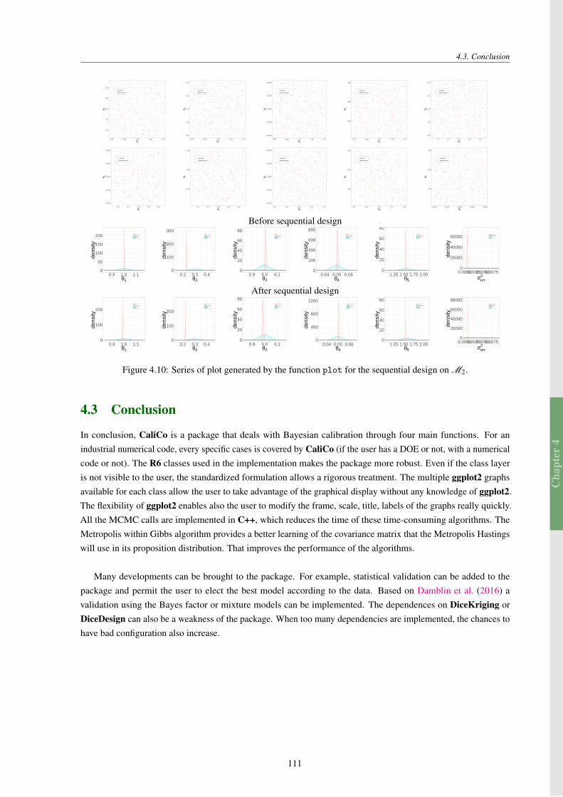
Cha

pter

4

4.3. Conclusion

0.1

0.2

0.3

0.4

0.5

0.90 0.95 1.00 1.05 1.10θ1

θ 2

Initial DOE

Additional points

5.8

5.9

6.0

6.1

6.2

0.90 0.95 1.00 1.05 1.10θ1

θ 3

Initial DOE

Additional points

0.040

0.045

0.050

0.055

0.060

0.90 0.95 1.00 1.05 1.10θ1

θ 4

Initial DOE

Additional points

1.52

1.56

1.60

0.90 0.95 1.00 1.05 1.10θ1

θ 5

Initial DOE

Additional points

5.8

5.9

6.0

6.1

6.2

0.1 0.2 0.3 0.4 0.5θ2

θ 3

Initial DOE

Additional points

0.040

0.045

0.050

0.055

0.060

0.1 0.2 0.3 0.4 0.5θ2

θ 4

Initial DOE

Additional points

1.52

1.56

1.60

0.1 0.2 0.3 0.4 0.5θ2

θ 5

Initial DOE

Additional points

0.040

0.045

0.050

0.055

0.060

5.8 5.9 6.0 6.1 6.2θ3

θ 4

Initial DOE

Additional points

1.52

1.56

1.60

5.8 5.9 6.0 6.1 6.2θ3

θ 5

Initial DOE

Additional points

1.52

1.56

1.60

0.040 0.045 0.050 0.055 0.060θ4

θ 5

Initial DOE

Additional points

Before sequential design

0

50

100

150

200

0.9 1.0 1.1θ1

dens

ity

posterior

prior

0

100

200

300

0.2 0.3 0.4θ2

dens

ity

posterior

prior

0

20

40

60

80

5.9 6.0 6.1θ3

dens

ityposterior

prior

0

200

400

600

800

0.04 0.05 0.06θ4

dens

ity

posterior

prior

0

20

40

60

80

1.25 1.50 1.75 2.00θ5

dens

ity

posterior

prior

0

20000

40000

60000

0.00000.00250.00500.0075σerr

2

dens

ity

posterior

prior

After sequential design

0

100

200

0.9 1.0 1.1θ1

dens

ity

posterior

prior

0

100

200

0.2 0.3 0.4θ2

dens

ity

posterior

prior

0

20

40

60

80

5.9 6.0 6.1θ3

dens

ity

posterior

prior

0

400

800

1200

0.04 0.05 0.06θ4

dens

ityposterior

prior

0

20

40

60

80

1.25 1.50 1.75 2.00θ5

dens

ity

posterior

prior

0

20000

40000

60000

80000

0.00000.00250.00500.0075σerr

2

dens

ity

posterior

prior

Figure 4.10: Series of plot generated by the function plot for the sequential design on M2.

4.3 Conclusion

In conclusion, CaliCo is a package that deals with Bayesian calibration through four main functions. For anindustrial numerical code, every specific cases is covered by CaliCo (if the user has a DOE or not, with a numericalcode or not). The R6 classes used in the implementation makes the package more robust. Even if the class layeris not visible to the user, the standardized formulation allows a rigorous treatment. The multiple ggplot2 graphsavailable for each class allow the user to take advantage of the graphical display without any knowledge of ggplot2.The flexibility of ggplot2 enables also the user to modify the frame, scale, title, labels of the graphs really quickly.All the MCMC calls are implemented in C++, which reduces the time of these time-consuming algorithms. TheMetropolis within Gibbs algorithm provides a better learning of the covariance matrix that the Metropolis Hastingswill use in its proposition distribution. That improves the performance of the algorithms.

Many developments can be brought to the package. For example, statistical validation can be added to thepackage and permit the user to elect the best model according to the data. Based on Damblin et al. (2016) avalidation using the Bayes factor or mixture models can be implemented. The dependences on DiceKriging orDiceDesign can also be a weakness of the package. When too many dependencies are implemented, the chances tohave bad configuration also increase.

111

Cha

pter

5

CHAPTER5PERFORMANCE MONITORING ON A

LARGE PV PLANT

5.1 Sensitivity analysis . . . . . . . . . . . . . . . . . . . . . . . . . . . . . . . . . . . . . . . . . . 1135.2 Prior densities . . . . . . . . . . . . . . . . . . . . . . . . . . . . . . . . . . . . . . . . . . . . . 1175.3 Propagation of uncertainties . . . . . . . . . . . . . . . . . . . . . . . . . . . . . . . . . . . . . 1185.4 Bayesian calibration . . . . . . . . . . . . . . . . . . . . . . . . . . . . . . . . . . . . . . . . . . 118

5.4.1 Statistical models . . . . . . . . . . . . . . . . . . . . . . . . . . . . . . . . . . . . . . . 1185.4.2 Modular estimation and likelihoods . . . . . . . . . . . . . . . . . . . . . . . . . . . . . 1205.4.3 Application to the PV plant . . . . . . . . . . . . . . . . . . . . . . . . . . . . . . . . . 121

This chapter concerns the study of a PV plant built and maintained by EDF. The precise location is not given anddata are normalized for a confidentiality matter. Mainly, the numerical code, based on the one diode modeling(among the advanced physical models presented in Section 1.3.2) is considered in this chapter. Particularly, thenumerical code introduced in Section 1.4.4 is used to complete the study in a performance monitoring context.Based on actual production and meteorological data over one year, code calibration better assesses the uncertaintieson the parameters input of the Dymola code to this specific case. Once calibration has been run, the code with thenew parameter distributions, could predict better the power for a next period of time. The business plan initiallyconceived on the prior parameter distributions, can then be reviewed and the price of electricity adapted to thenew estimated power. This chapter presents first the numerical code and the sensitivity analysis performed onthe 26 parameters. The prior distributions of the parameters are also presented which leads to a propagation ofuncertainties a priori. Then calibration, in this particular case, is performed but the following issues differ fromprevious chapters. Indeed, the Dymola code outputs are time series and dealing with multidimensional output incalibration requires additional work.

5.1 Sensitivity analysis

The Dymola code, as presented in Section 1.4.4, is more accurate in the prediction of a large PV plant productionthan the code used in Chapter 3. Indeed, one of the limitations of the code used to compare calibration models,is to over estimate the power when shades appear. This case scenario occurs every days in a large PV plantconfiguration because when the sun comes up, the panel in the first raw automatically creates a shade on theone behind. However, because it adds implicit equations that need to be numerically solved, such a developmenthas the effect to slow down the code speed. Moreover, the code estimates the power of the PV plant over ayear and produces a time series of 15,858 points. Applying regular sensitivity analysis (as it was the case forthe methods presented in Section 2.1) is more complicated because it has to take into account the behavior ofthe code on the whole time frame and not only in the instantaneous time. To overcome these issues, the same

113

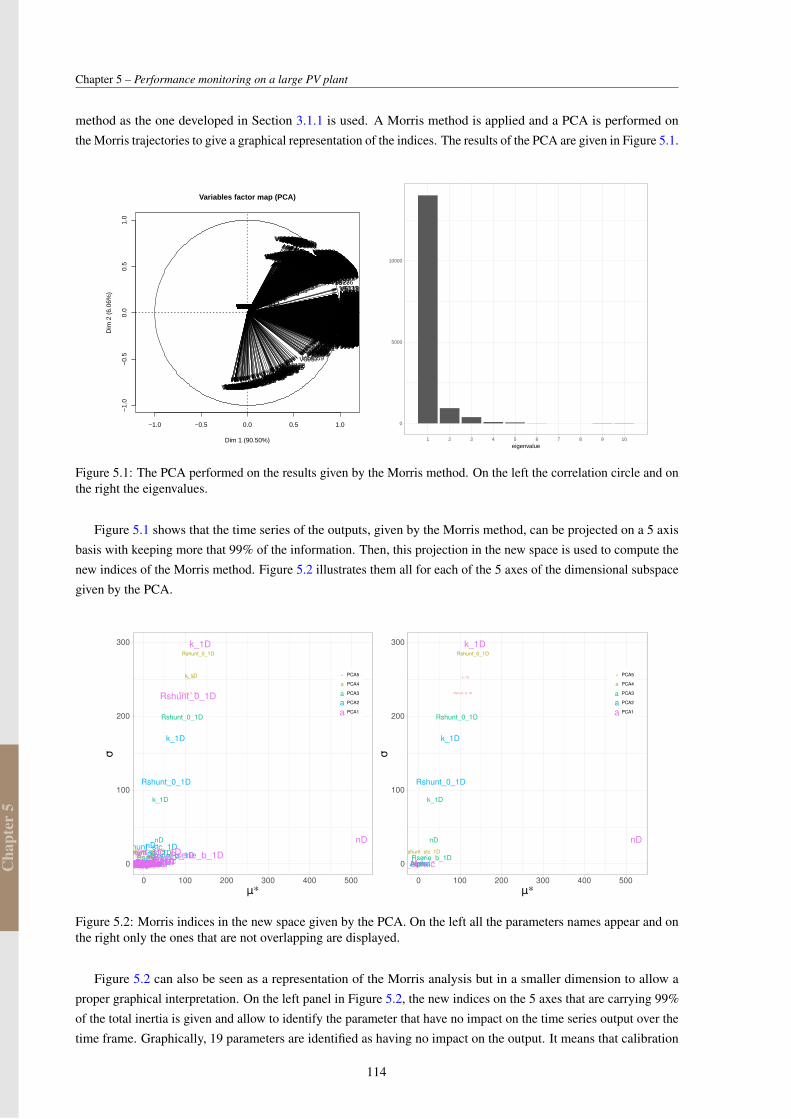
Cha

pter

5

Chapter 5 – Performance monitoring on a large PV plant

method as the one developed in Section 3.1.1 is used. A Morris method is applied and a PCA is performed onthe Morris trajectories to give a graphical representation of the indices. The results of the PCA are given in Figure 5.1.

−1.0 −0.5 0.0 0.5 1.0

−1.

0−

0.5

0.0

0.5

1.0

Variables factor map (PCA)

Dim 1 (90.50%)

Dim

2 (

6.06

%)

V1V2

V3V4

V5

V6V7V8V9V10V11V12V13V14

V15V16V17V18V19V20V21V22V23V24V25V26V27

V28V29V30V31V32V33V34V35

V36

V37

V38

V39

V40

V41

V42V43V44V45V46V47V48V49V50V51V52V53V54V55V56V57V58V59V60V61V62V63

V64V65

V66V67V68V69V70V71V72V73V74

V75V76V77

V78

V79

V80

V81V82

V83

V84V85V86V87V88V89V90V91

V92

V93V94V95V96V97V98V99

V100

V101

V102V103

V104

V105V106V107V108V109V110V111

V112V113V114V115V116V117

V118V119

V120

V121V122V123

V124V125

V126

V127V128V129V130

V131V132V133V134

V135V136V137

V138

V139V140V141

V142

V143V144

V145V146V147V148

V149V150V151V152V153V154V155V156

V157

V158

V159

V160V161V162V163V164V165V166V167V168V169V170V171V172V173V174V175V176V177V178V179V180V181V182V183V184V185V186V187V188V189V190V191V192V193V194V195

V196V197

V198

V199

V200

V201

V202

V203V204V205

V206

V207V208

V209

V210V211V212

V213V214

V215V216V217

V218V219V220V221V222V223V224V225V226V227V228V229V230

V231

V232

V233V234V235V236

V237

V238V239

V240

V241V242V243V244V245V246V247

V248V249V250V251

V252V253V254V255V256

V257V258V259V260

V261V262

V263

V264V265V266

V267V268V269V270V271

V272

V273V274

V275V276

V277

V278V279V280V281V282

V283

V284

V285V286V287V288

V289

V290

V291V292V293V294V295

V296

V297

V298V299

V300

V301

V302V303V304

V305V306V307V308

V309V310V311

V312V313V314

V315

V316V317V318

V319

V320

V321

V322

V323

V324

V325V326

V327

V328

V329

V330V331V332V333V334V335

V336

V337V338

V339V340V341

V342

V343V344V345

V346V347V348

V349

V350

V351V352V353V354V355V356V357

V358V359V360V361V362V363

V364V365V366

V367

V368

V369V370V371V372V373

V374

V375V376V377

V378V379

V380V381V382V383

V384

V385V386V387

V388V389

V390

V391

V392V393V394

V395

V396

V397V398

V399

V400V401

V402V403V404

V405

V406V407

V408

V409V410

V411V412V413

V414

V415

V416

V417V418V419V420V421

V422

V423

V424

V425

V426V427V428V429V430V431V432V433V434V435V436V437V438V439V440V441V442V443V444V445V446V447V448V449V450V451V452V453V454V455V456V457V458V459V460V461

V462

V463V464

V465

V466

V467V468V469V470V471V472V473V474V475V476V477V478V479V480V481V482V483V484V485V486V487V488V489V490V491V492V493V494V495V496V497V498V499V500V501V502

V503

V504

V505

V506

V507V508V509V510V511V512V513V514V515V516V517V518V519V520

V521V522

V523V524V525V526V527V528V529V530V531V532V533V534V535V536V537V538

V539

V540V541V542V543V544

V545

V546

V547

V548V549V550V551V552V553V554

V555

V556V557V558

V559V560V561

V562V563

V564

V565

V566

V567V568

V569

V570V571

V572

V573V574

V575V576V577

V578

V579

V580

V581V582

V583

V584V585V586V587

V588V589V590V591V592V593V594V595V596V597V598V599V600

V601V602V603V604V605

V606

V607

V608

V609V610

V611

V612V613

V614

V615

V616

V617

V618V619

V620V621

V622

V623

V624

V625

V626

V627V628

V629V630V631

V632V633V634

V635V636V637V638

V639

V640V641

V642V643V644V645V646V647V648V649V650V651V652V653V654V655V656V657V658

V659

V660

V661

V662

V663

V664V665V666V667V668V669V670V671V672V673V674V675V676V677V678V679V680V681V682V683V684V685V686V687V688V689V690V691V692V693V694V695V696V697V698V699

V700

V701

V702

V703V704

V705V706V707V708V709V710V711

V712V713

V714

V715V716

V717

V718V719V720V721V722

V723V724

V725

V726

V727

V728

V729V730V731V732

V733V734V735V736V737

V738

V739

V740V741

V742

V743

V744

V745V746V747V748V749V750V751V752V753V754V755V756V757V758V759V760V761V762V763V764V765V766V767V768V769V770V771V772V773V774V775V776V777V778V779V780V781

V782

V783

V784V785V786V787V788V789V790V791V792V793V794V795V796V797V798V799V800V801V802V803V804V805V806V807V808V809V810V811V812V813V814V815V816V817V818V819V820V821V822V823

V824V825V826V827V828V829V830V831V832V833V834V835V836V837V838V839V840V841V842V843V844V845V846V847V848V849V850V851V852V853V854V855V856V857V858V859V860V861V862V863

V864V865V866V867V868V869V870V871V872V873V874V875V876V877V878V879V880V881V882V883V884V885V886V887V888V889V890V891V892V893V894V895V896V897V898V899V900V901

V902V903

V904

V905V906

V907

V908

V909

V910V911V912V913V914V915V916V917V918V919V920V921V922V923V924V925V926V927V928V929V930V931V932V933V934V935V936V937V938V939V940V941V942V943

V944

V945

V946

V947

V948

V949V950

V951

V952V953V954V955V956V957V958V959V960V961V962V963V964V965V966

V967V968

V969V970

V971V972V973V974V975V976V977V978V979V980V981V982V983V984

V985

V986V987V988

V989V990V991V992

V993

V994V995V996V997V998V999V1000V1001

V1002V1003V1004V1005V1006V1007V1008V1009V1010V1011V1012V1013V1014

V1015V1016V1017V1018V1019V1020V1021V1022V1023

V1024

V1025V1026V1027

V1028V1029V1030V1031

V1032

V1033

V1034V1035V1036V1037V1038V1039V1040V1041V1042V1043V1044V1045

V1046V1047V1048V1049V1050V1051V1052V1053V1054V1055V1056V1057V1058V1059V1060V1061

V1062V1063

V1064V1065V1066V1067

V1068

V1069

V1070V1071V1072V1073V1074V1075V1076V1077V1078V1079

V1080V1081

V1082V1083

V1084V1085

V1086V1087

V1088V1089V1090

V1091

V1092V1093V1094V1095V1096V1097

V1098V1099V1100

V1101

V1102V1103

V1104V1105V1106V1107

V1108

V1109

V1110V1111

V1112V1113V1114

V1115V1116V1117V1118V1119V1120V1121V1122V1123V1124V1125V1126V1127V1128V1129V1130V1131V1132V1133V1134V1135V1136V1137V1138V1139V1140V1141V1142V1143V1144V1145V1146V1147

V1148

V1149

V1150V1151

V1152

V1153V1154V1155V1156V1157V1158V1159V1160V1161V1162V1163V1164V1165V1166V1167V1168V1169V1170V1171V1172V1173V1174V1175V1176V1177V1178V1179V1180V1181V1182V1183V1184V1185V1186V1187V1188V1189

V1190

V1191

V1192V1193

V1194

V1195V1196V1197V1198V1199V1200V1201V1202V1203V1204V1205V1206V1207V1208V1209V1210V1211V1212V1213V1214V1215V1216V1217V1218V1219V1220V1221V1222V1223V1224V1225V1226V1227V1228V1229V1230V1231V1232

V1233

V1234V1235

V1236

V1237V1238V1239V1240V1241V1242V1243V1244V1245V1246V1247V1248V1249V1250V1251V1252V1253V1254V1255V1256V1257V1258V1259V1260V1261V1262V1263V1264V1265V1266V1267V1268V1269V1270V1271V1272V1273V1274

V1275

V1276V1277V1278

V1279

V1280V1281V1282V1283V1284V1285V1286V1287V1288V1289

V1290V1291V1292V1293V1294V1295V1296V1297V1298V1299V1300V1301V1302V1303V1304V1305V1306V1307V1308V1309V1310V1311V1312V1313V1314V1315V1316V1317

V1318

V1319V1320

V1321

V1322V1323V1324V1325V1326V1327V1328V1329V1330V1331V1332V1333V1334V1335V1336V1337V1338V1339V1340V1341V1342V1343V1344V1345V1346V1347V1348

V1349V1350V1351V1352V1353V1354V1355V1356V1357V1358

V1359

V1360

V1361

V1362V1363

V1364

V1365V1366V1367V1368V1369V1370V1371V1372V1373V1374V1375V1376V1377V1378V1379V1380V1381V1382

V1383

V1384

V1385V1386V1387V1388

V1389V1390V1391V1392V1393V1394V1395V1396V1397V1398V1399V1400V1401

V1402

V1403

V1404

V1405V1406

V1407

V1408V1409V1410V1411V1412V1413V1414V1415V1416V1417V1418V1419V1420V1421V1422V1423V1424V1425V1426V1427V1428V1429V1430V1431V1432V1433V1434V1435V1436V1437V1438V1439V1440V1441V1442V1443V1444V1445

V1446

V1447

V1448V1449

V1450

V1451

V1452V1453V1454V1455

V1456V1457V1458V1459V1460V1461

V1462V1463V1464V1465

V1466V1467V1468

V1469

V1470V1471

V1472V1473V1474V1475V1476V1477

V1478V1479

V1480

V1481

V1482V1483

V1484

V1485

V1486V1487

V1488

V1489

V1490

V1491

V1492

V1493V1494V1495V1496V1497V1498

V1499V1500

V1501V1502V1503V1504V1505V1506V1507V1508V1509V1510V1511

V1512

V1513V1514V1515

V1516V1517V1518V1519V1520V1521V1522V1523V1524V1525V1526V1527V1528

V1529

V1530V1531V1532

V1533V1534V1535

V1536

V1537V1538V1539V1540

V1541V1542

V1543

V1544V1545V1546V1547V1548V1549

V1550V1551

V1552V1553V1554V1555V1556

V1557V1558V1559V1560V1561V1562V1563

V1564

V1565

V1566

V1567V1568

V1569V1570V1571V1572

V1573V1574V1575V1576

V1577

V1578V1579V1580V1581V1582V1583V1584V1585V1586V1587V1588V1589V1590V1591V1592V1593V1594V1595V1596V1597V1598V1599V1600V1601V1602V1603V1604V1605V1606V1607V1608V1609V1610V1611V1612V1613V1614V1615

V1616

V1617

V1618

V1619

V1620

V1621V1622V1623V1624V1625V1626V1627V1628V1629V1630V1631V1632V1633V1634V1635V1636V1637V1638V1639V1640V1641V1642V1643V1644V1645V1646V1647V1648V1649V1650V1651V1652V1653V1654

V1655

V1656V1657V1658V1659

V1660V1661

V1662V1663

V1664

V1665V1666V1667V1668V1669V1670V1671V1672V1673V1674V1675V1676V1677V1678V1679V1680V1681V1682V1683V1684V1685V1686V1687V1688

V1689

V1690

V1691

V1692

V1693

V1694V1695

V1696

V1697

V1698V1699V1700V1701V1702 V1703

V1704

V1705V1706V1707V1708V1709V1710V1711V1712V1713V1714V1715V1716V1717V1718V1719V1720V1721V1722V1723V1724V1725V1726V1727

V1728V1729V1730V1731V1732V1733V1734V1735V1736V1737V1738V1739V1740V1741

V1742

V1743V1744

V1745

V1746

V1747

V1748V1749V1750V1751V1752V1753V1754V1755V1756V1757V1758V1759V1760V1761

V1762V1763V1764V1765V1766V1767V1768V1769V1770V1771V1772V1773

V1774

V1775

V1776

V1777V1778V1779V1780

V1781

V1782

V1783

V1784

V1785

V1786

V1787

V1788

V1789

V1790V1791V1792V1793V1794V1795V1796V1797V1798V1799V1800V1801V1802V1803V1804V1805V1806V1807

V1808V1809V1810

V1811V1812

V1813V1814

V1815

V1816V1817

V1818V1819V1820V1821V1822V1823V1824V1825V1826V1827V1828V1829

V1830

V1831V1832 V1833V1834V1835V1836V1837V1838V1839V1840V1841V1842V1843V1844V1845V1846V1847V1848V1849

V1850V1851V1852V1853V1854V1855V1856V1857V1858

V1859

V1860V1861

V1862V1863

V1864V1865V1866V1867V1868V1869V1870V1871V1872

V1873

V1874V1875

V1876

V1877

V1878V1879

V1880V1881

V1882

V1883V1884

V1885

V1886V1887V1888

V1889V1890V1891V1892

V1893V1894

V1895

V1896V1897

V1898V1899

V1900

V1901

V1902

V1903V1904V1905V1906

V1907V1908V1909V1910V1911V1912V1913V1914

V1915

V1916V1917

V1918V1919

V1920

V1921V1922V1923V1924V1925V1926V1927V1928V1929V1930V1931V1932

V1933V1934

V1935

V1936V1937

V1938

V1939V1940

V1941V1942

V1943V1944

V1945

V1946V1947V1948

V1949V1950V1951V1952V1953V1954

V1955V1956V1957

V1958

V1959

V1960

V1961

V1962V1963

V1964V1965V1966

V1967V1968V1969V1970V1971V1972V1973V1974V1975V1976

V1977

V1978

V1979

V1980V1981

V1982

V1983V1984V1985V1986V1987V1988

V1989

V1990V1991V1992V1993V1994V1995V1996V1997

V1998

V1999V2000

V2001V2002

V2003

V2004V2005

V2006V2007V2008V2009V2010

V2011

V2012V2013

V2014V2015

V2016V2017

V2018

V2019V2020V2021V2022V2023V2024V2025V2026V2027

V2028

V2029V2030V2031

V2032V2033

V2034

V2035V2036V2037

V2038

V2039

V2040V2041V2042V2043

V2044V2045V2046

V2047

V2048

V2049

V2050V2051V2052V2053V2054V2055V2056V2057

V2058

V2059

V2060

V2061

V2062 V2063

V2064

V2065

V2066

V2067

V2068V2069

V2070V2071

V2072V2073V2074V2075V2076V2077

V2078

V2079

V2080

V2081

V2082V2083

V2084V2085

V2086V2087

V2088V2089V2090

V2091

V2092V2093V2094

V2095

V2096

V2097V2098

V2099V2100

V2101

V2102V2103

V2104

V2105

V2106V2107

V2108

V2109

V2110

V2111

V2112

V2113

V2114V2115V2116V2117V2118

V2119V2120V2121V2122V2123V2124V2125

V2126

V2127

V2128V2129

V2130

V2131V2132V2133V2134V2135V2136V2137V2138V2139V2140V2141V2142V2143

V2144V2145V2146V2147V2148V2149V2150V2151V2152V2153V2154V2155

V2156V2157V2158V2159V2160V2161V2162

V2163V2164V2165V2166V2167

V2168

V2169V2170V2171

V2172

V2173

V2174

V2175V2176V2177

V2178V2179

V2180V2181V2182V2183V2184V2185V2186V2187V2188V2189V2190V2191V2192V2193V2194V2195V2196V2197V2198V2199V2200V2201V2202

V2203V2204V2205V2206V2207V2208V2209

V2210

V2211

V2212V2213

V2214V2215V2216V2217

V2218V2219V2220

V2221

V2222

V2223V2224V2225V2226V2227V2228

V2229

V2230

V2231

V2232V2233

V2234

V2235

V2236V2237V2238V2239V2240

V2241

V2242V2243

V2244

V2245V2246V2247V2248V2249V2250V2251

V2252

V2253

V2254

V2255

V2256

V2257

V2258V2259V2260

V2261

V2262

V2263

V2264

V2265V2266V2267V2268V2269V2270V2271V2272V2273V2274V2275V2276V2277V2278V2279V2280V2281

V2282V2283

V2284

V2285

V2286

V2287

V2288V2289V2290V2291V2292V2293V2294V2295V2296V2297V2298V2299V2300V2301V2302V2303

V2304

V2305

V2306

V2307

V2308

V2309V2310V2311V2312V2313V2314V2315V2316V2317V2318V2319V2320V2321V2322

V2323V2324V2325V2326V2327V2328V2329V2330V2331V2332V2333V2334V2335V2336V2337V2338V2339V2340V2341V2342V2343V2344V2345V2346V2347V2348V2349

V2350

V2351

V2352

V2353

V2354V2355V2356V2357V2358V2359V2360V2361V2362V2363V2364V2365V2366V2367V2368V2369V2370V2371V2372V2373V2374V2375V2376V2377V2378V2379V2380V2381

V2382

V2383V2384V2385V2386V2387V2388V2389V2390V2391V2392V2393

V2394

V2395

V2396

V2397

V2398

V2399

V2400V2401V2402V2403V2404V2405V2406V2407V2408

V2409V2410V2411V2412V2413

V2414V2415

V2416V2417V2418

V2419

V2420V2421

V2422V2423V2424V2425V2426V2427V2428V2429V2430V2431V2432V2433V2434V2435V2436V2437V2438

V2439

V2440

V2441V2442

V2443

V2444V2445V2446V2447V2448V2449V2450V2451V2452V2453V2454V2455V2456V2457V2458V2459V2460V2461V2462V2463V2464V2465V2466V2467V2468V2469V2470V2471V2472V2473V2474V2475V2476V2477V2478V2479V2480V2481V2482

V2483

V2484V2485

V2486

V2487

V2488

V2489V2490V2491V2492V2493V2494V2495V2496V2497V2498V2499

V2500

V2501

V2502

V2503

V2504V2505

V2506V2507V2508

V2509

V2510

V2511

V2512V2513V2514V2515V2516V2517V2518V2519V2520V2521V2522V2523

V2524V2525V2526

V2527V2528

V2529

V2530

V2531

V2532

V2533

V2534V2535V2536V2537V2538V2539V2540V2541V2542V2543V2544V2545V2546V2547V2548V2549V2550V2551V2552V2553V2554V2555V2556V2557V2558V2559V2560V2561V2562V2563V2564V2565V2566V2567V2568V2569V2570V2571V2572V2573

V2574

V2575V2576V2577

V2578

V2579

V2580

V2581

V2582

V2583V2584

V2585

V2586V2587V2588

V2589V2590V2591

V2592

V2593

V2594

V2595V2596

V2597V2598V2599V2600V2601V2602V2603

V2604V2605V2606V2607V2608V2609V2610V2611V2612V2613V2614V2615V2616

V2617

V2618

V2619V2620V2621

V2622

V2623V2624V2625V2626V2627V2628V2629V2630V2631V2632V2633V2634V2635V2636V2637V2638V2639V2640V2641V2642V2643V2644V2645V2646V2647V2648V2649V2650V2651V2652V2653V2654V2655V2656V2657V2658V2659V2660V2661V2662V2663

V2664

V2665

V2666V2667V2668

V2669

V2670

V2671V2672V2673V2674V2675V2676V2677V2678V2679V2680V2681V2682V2683V2684V2685V2686V2687V2688V2689V2690V2691V2692V2693V2694V2695V2696V2697V2698V2699V2700V2701V2702V2703V2704V2705V2706V2707V2708V2709V2710

V2711

V2712

V2713V2714

V2715

V2716

V2717V2718V2719V2720V2721V2722V2723V2724V2725V2726V2727V2728V2729V2730V2731V2732V2733V2734V2735V2736V2737V2738V2739V2740V2741V2742V2743V2744V2745V2746V2747V2748V2749V2750V2751V2752V2753V2754V2755V2756

V2757

V2758

V2759

V2760V2761

V2762

V2763V2764V2765V2766V2767V2768V2769V2770V2771V2772V2773V2774V2775V2776V2777V2778V2779V2780

V2781V2782V2783V2784V2785V2786V2787V2788V2789

V2790V2791V2792V2793V2794

V2795V2796V2797V2798V2799V2800V2801V2802

V2803

V2804

V2805

V2806

V2807

V2808V2809V2810V2811V2812

V2813

V2814V2815V2816V2817

V2818V2819V2820V2821V2822V2823V2824V2825V2826V2827V2828V2829

V2830

V2831V2832V2833

V2834V2835V2836V2837V2838

V2839V2840V2841V2842V2843V2844V2845

V2846

V2847

V2848

V2849V2850V2851

V2852

V2853

V2854

V2855V2856V2857V2858V2859V2860V2861V2862V2863V2864

V2865V2866

V2867

V2868

V2869

V2870V2871

V2872

V2873

V2874V2875

V2876

V2877V2878V2879V2880V2881V2882

V2883V2884V2885V2886V2887V2888V2889V2890V2891V2892V2893V2894V2895V2896

V2897V2898

V2899

V2900

V2901

V2902V2903V2904V2905V2906V2907V2908V2909V2910V2911

V2912V2913V2914

V2915

V2916V2917V2918

V2919

V2920

V2921

V2922V2923V2924

V2925V2926V2927V2928V2929V2930V2931V2932V2933V2934V2935V2936V2937V2938V2939V2940V2941V2942V2943

V2944

V2945

V2946V2947

V2948

V2949

V2950V2951V2952V2953V2954V2955V2956V2957V2958V2959V2960V2961V2962V2963V2964V2965V2966V2967V2968V2969V2970V2971V2972V2973V2974V2975V2976V2977V2978V2979V2980V2981V2982V2983V2984V2985V2986V2987V2988V2989V2990

V2991

V2992

V2993

V2994

V2995

V2996

V2997V2998V2999V3000V3001V3002V3003

V3004V3005V3006V3007

V3008

V3009V3010V3011V3012V3013V3014

V3015V3016V3017V3018V3019V3020V3021V3022V3023V3024

V3025V3026V3027V3028V3029V3030V3031V3032V3033V3034V3035V3036

V3037V3038V3039

V3040

V3041

V3042V3043V3044

V3045V3046V3047V3048V3049V3050V3051V3052V3053

V3054

V3055

V3056

V3057V3058V3059

V3060V3061

V3062

V3063V3064V3065

V3066

V3067

V3068V3069

V3070

V3071V3072V3073

V3074

V3075V3076V3077V3078V3079V3080V3081V3082V3083V3084

V3085V3086V3087

V3088V3089

V3090

V3091

V3092V3093V3094V3095V3096V3097V3098V3099V3100V3101V3102V3103V3104V3105V3106V3107

V3108V3109V3110V3111V3112V3113V3114V3115V3116V3117V3118V3119V3120V3121V3122

V3123

V3124V3125V3126V3127V3128V3129V3130

V3131

V3132V3133V3134V3135V3136

V3137V3138

V3139

V3140V3141V3142V3143

V3144

V3145

V3146V3147

V3148V3149V3150V3151V3152V3153V3154V3155V3156V3157V3158

V3159

V3160V3161V3162V3163V3164

V3165V3166

V3167

V3168

V3169V3170V3171

V3172

V3173V3174V3175V3176V3177V3178V3179

V3180V3181

V3182

V3183

V3184

V3185V3186V3187V3188

V3189

V3190V3191V3192V3193V3194V3195V3196V3197V3198V3199V3200V3201V3202V3203V3204V3205V3206V3207V3208V3209V3210V3211V3212V3213V3214V3215V3216V3217V3218V3219V3220V3221V3222V3223V3224V3225V3226V3227

V3228

V3229V3230

V3231

V3232

V3233V3234

V3235

V3236V3237V3238V3239

V3240V3241

V3242V3243

V3244

V3245V3246V3247V3248V3249

V3250V3251V3252V3253V3254V3255

V3256V3257V3258V3259V3260

V3261V3262V3263

V3264V3265V3266V3267V3268V3269V3270V3271V3272V3273V3274

V3275

V3276V3277V3278

V3279

V3280

V3281

V3282

V3283V3284V3285V3286V3287V3288V3289V3290V3291V3292

V3293

V3294

V3295V3296

V3297V3298V3299V3300

V3301

V3302V3303V3304

V3305

V3306V3307V3308V3309V3310

V3311V3312V3313V3314V3315V3316

V3317V3318V3319

V3320

V3321

V3322

V3323V3324

V3325

V3326

V3327

V3328

V3329V3330V3331V3332V3333V3334V3335V3336V3337V3338

V3339V3340V3341V3342V3343V3344

V3345V3346V3347V3348

V3349V3350V3351

V3352V3353V3354V3355V3356

V3357

V3358

V3359V3360

V3361

V3362

V3363

V3364

V3365

V3366

V3367V3368V3369V3370

V3371

V3372V3373

V3374

V3375V3376V3377V3378V3379V3380V3381V3382V3383V3384

V3385

V3386V3387V3388V3389V3390V3391

V3392

V3393V3394V3395V3396V3397V3398V3399V3400V3401V3402V3403V3404V3405V3406V3407V3408V3409V3410V3411V3412V3413V3414V3415

V3416V3417V3418

V3419

V3420

V3421

V3422V3423V3424V3425V3426V3427V3428V3429V3430V3431V3432V3433V3434V3435V3436V3437V3438V3439V3440V3441V3442V3443V3444V3445V3446V3447V3448V3449V3450V3451V3452V3453V3454V3455V3456V3457V3458V3459V3460V3461V3462

V3463

V3464V3465

V3466V3467V3468

V3469V3470

V3471V3472V3473V3474V3475V3476V3477V3478V3479V3480

V3481V3482

V3483

V3484V3485

V3486V3487

V3488V3489V3490

V3491V3492

V3493

V3494V3495V3496V3497V3498V3499V3500V3501V3502V3503V3504V3505V3506V3507V3508V3509V3510V3511V3512

V3513

V3514V3515V3516V3517

V3518

V3519V3520

V3521

V3522V3523V3524V3525

V3526V3527V3528V3529

V3530V3531

V3532V3533V3534

V3535

V3536V3537V3538V3539

V3540

V3541V3542V3543

V3544V3545V3546V3547V3548V3549V3550V3551V3552V3553V3554V3555V3556

V3557V3558V3559

V3560

V3561

V3562

V3563V3564

V3565

V3566

V3567V3568V3569V3570V3571V3572V3573V3574

V3575

V3576

V3577

V3578V3579V3580V3581V3582V3583V3584V3585V3586

V3587V3588V3589V3590

V3591V3592V3593V3594V3595V3596V3597V3598V3599

V3600V3601V3602V3603V3604V3605V3606V3607

V3608

V3609

V3610

V3611

V3612V3613

V3614V3615V3616

V3617V3618V3619V3620V3621V3622

V3623V3624

V3625

V3626V3627

V3628V3629V3630

V3631

V3632V3633

V3634

V3635V3636

V3637V3638V3639V3640V3641V3642V3643V3644V3645V3646V3647V3648

V3649V3650V3651V3652V3653V3654V3655V3656V3657V3658

V3659

V3660

V3661

V3662

V3663

V3664

V3665

V3666V3667V3668V3669V3670V3671

V3672

V3673

V3674

V3675V3676

V3677

V3678V3679V3680

V3681V3682V3683

V3684V3685

V3686V3687

V3688V3689V3690V3691V3692V3693V3694

V3695V3696V3697V3698V3699V3700V3701V3702V3703V3704V3705V3706V3707V3708

V3709

V3710

V3711V3712

V3713

V3714

V3715

V3716V3717V3718V3719V3720V3721V3722V3723V3724V3725V3726V3727V3728V3729V3730V3731V3732V3733V3734V3735V3736V3737V3738V3739V3740V3741V3742V3743V3744V3745V3746V3747V3748V3749V3750V3751V3752V3753V3754V3755V3756V3757V3758

V3759

V3760

V3761

V3762

V3763

V3764

V3765

V3766V3767V3768V3769V3770V3771V3772V3773V3774V3775V3776V3777V3778V3779V3780V3781V3782V3783V3784V3785V3786V3787V3788V3789V3790V3791V3792V3793V3794V3795V3796V3797V3798V3799V3800V3801V3802V3803V3804V3805V3806V3807V3808

V3809

V3810

V3811

V3812

V3813

V3814

V3815

V3816V3817V3818V3819V3820V3821V3822V3823V3824V3825V3826V3827V3828V3829V3830V3831V3832V3833V3834V3835V3836V3837V3838V3839V3840V3841V3842V3843V3844V3845V3846V3847V3848V3849V3850V3851V3852V3853V3854V3855V3856V3857V3858

V3859

V3860

V3861V3862

V3863

V3864

V3865

V3866V3867V3868V3869V3870V3871V3872V3873

V3874

V3875

V3876

V3877V3878V3879V3880

V3881V3882V3883V3884V3885V3886V3887V3888V3889V3890V3891V3892V3893

V3894V3895

V3896V3897

V3898

V3899V3900V3901V3902V3903V3904V3905V3906V3907V3908

V3909

V3910

V3911

V3912V3913V3914V3915

V3916

V3917V3918V3919V3920V3921V3922V3923V3924V3925V3926

V3927V3928

V3929V3930V3931V3932

V3933V3934

V3935V3936V3937

V3938

V3939V3940

V3941

V3942V3943V3944V3945V3946V3947V3948V3949V3950V3951V3952V3953V3954V3955V3956

V3957

V3958

V3959 V3960V3961

V3962

V3963V3964V3965V3966

V3967

V3968

V3969

V3970

V3971V3972V3973V3974

V3975

V3976

V3977V3978

V3979

V3980

V3981

V3982

V3983

V3984

V3985

V3986

V3987

V3988

V3989

V3990V3991V3992

V3993V3994V3995V3996V3997V3998V3999V4000V4001V4002V4003V4004

V4005V4006

V4007

V4008V4009

V4010V4011

V4012

V4013

V4014V4015V4016V4017

V4018V4019

V4020V4021

V4022V4023V4024V4025

V4026

V4027V4028

V4029

V4030V4031V4032

V4033V4034

V4035

V4036V4037V4038V4039V4040V4041V4042V4043V4044V4045V4046V4047V4048V4049V4050V4051

V4052

V4053V4054

V4055V4056

V4057V4058

V4059

V4060V4061V4062V4063V4064V4065

V4066V4067V4068V4069V4070V4071V4072V4073V4074

V4075V4076

V4077V4078V4079V4080V4081V4082V4083V4084V4085V4086V4087V4088V4089V4090V4091V4092V4093V4094V4095V4096V4097V4098V4099V4100V4101V4102

V4103

V4104V4105

V4106

V4107

V4108V4109

V4110

V4111V4112V4113V4114V4115V4116V4117V4118V4119V4120V4121V4122V4123V4124V4125V4126V4127V4128V4129V4130V4131V4132V4133V4134V4135V4136V4137V4138V4139V4140V4141V4142V4143V4144V4145V4146V4147V4148V4149V4150V4151V4152V4153

V4154

V4155V4156

V4157

V4158

V4159V4160

V4161V4162V4163V4164V4165V4166V4167V4168V4169V4170V4171V4172V4173V4174V4175V4176V4177V4178V4179V4180V4181V4182V4183V4184V4185V4186V4187V4188V4189V4190V4191V4192V4193V4194V4195V4196V4197V4198V4199V4200V4201V4202V4203

V4204

V4205V4206V4207

V4208

V4209V4210

V4211

V4212

V4213V4214V4215V4216V4217V4218V4219V4220V4221V4222V4223V4224V4225V4226V4227V4228V4229V4230V4231V4232V4233V4234V4235V4236V4237V4238V4239V4240V4241V4242V4243V4244V4245V4246V4247V4248V4249V4250V4251V4252V4253V4254V4255

V4256

V4257V4258

V4259V4260

V4261

V4262

V4263

V4264

V4265V4266V4267V4268V4269V4270V4271V4272V4273

V4274

V4275V4276

V4277V4278

V4279V4280

V4281V4282V4283V4284V4285V4286V4287V4288V4289V4290V4291V4292V4293V4294V4295V4296V4297V4298V4299

V4300V4301V4302V4303V4304V4305V4306

V4307

V4308V4309V4310

V4311V4312

V4313V4314

V4315

V4316V4317V4318V4319V4320V4321V4322V4323V4324V4325V4326V4327V4328

V4329V4330

V4331V4332V4333

V4334V4335

V4336V4337V4338V4339V4340V4341

V4342

V4343

V4344V4345V4346V4347V4348

V4349

V4350V4351

V4352V4353V4354V4355V4356V4357V4358

V4359

V4360V4361

V4362

V4363V4364

V4365

V4366V4367V4368V4369V4370V4371V4372V4373V4374

V4375V4376V4377V4378

V4379V4380V4381V4382

V4383V4384

V4385V4386V4387

V4388V4389V4390V4391

V4392V4393

V4394

V4395

V4396

V4397

V4398

V4399

V4400V4401V4402V4403V4404V4405V4406V4407V4408V4409

V4410

V4411

V4412

V4413V4414

V4415V4416

V4417

V4418V4419V4420V4421V4422V4423V4424V4425V4426V4427V4428V4429V4430V4431V4432V4433V4434V4435V4436V4437V4438V4439V4440V4441V4442V4443V4444V4445V4446V4447V4448V4449V4450V4451V4452V4453V4454V4455V4456V4457V4458V4459V4460V4461

V4462

V4463V4464

V4465V4466

V4467V4468

V4469

V4470

V4471V4472V4473V4474V4475V4476V4477V4478V4479V4480V4481V4482V4483V4484V4485V4486V4487V4488V4489V4490V4491V4492V4493V4494V4495V4496V4497V4498V4499V4500V4501V4502V4503V4504V4505V4506V4507V4508V4509V4510V4511V4512V4513

V4514

V4515V4516

V4517

V4518V4519

V4520V4521

V4522

V4523V4524V4525V4526V4527V4528V4529V4530V4531V4532V4533V4534V4535V4536V4537V4538V4539V4540V4541V4542V4543V4544V4545V4546V4547V4548V4549V4550V4551V4552V4553V4554V4555V4556V4557V4558V4559V4560V4561V4562V4563V4564V4565V4566

V4567

V4568V4569V4570

V4571

V4572

V4573V4574

V4575

V4576V4577V4578V4579V4580V4581V4582V4583V4584V4585V4586V4587V4588V4589V4590V4591V4592V4593V4594V4595V4596V4597V4598V4599V4600V4601V4602V4603V4604V4605V4606V4607V4608V4609V4610V4611V4612V4613V4614V4615V4616V4617V4618V4619

V4620

V4621V4622V4623

V4624

V4625

V4626V4627

V4628

V4629V4630V4631V4632V4633V4634V4635V4636V4637V4638V4639V4640V4641V4642V4643V4644V4645V4646V4647V4648V4649V4650V4651V4652V4653V4654V4655V4656V4657V4658V4659V4660V4661V4662V4663V4664V4665V4666V4667V4668V4669V4670V4671V4672

V4673

V4674V4675V4676V4677

V4678V4679V4680

V4681

V4682

V4683

V4684V4685V4686

V4687V4688V4689

V4690V4691V4692V4693V4694V4695V4696V4697V4698V4699V4700V4701V4702V4703V4704V4705V4706V4707V4708V4709V4710V4711V4712V4713V4714V4715V4716V4717V4718V4719V4720V4721V4722V4723V4724

V4725

V4726V4727

V4728

V4729

V4730

V4731V4732

V4733

V4734V4735V4736V4737V4738V4739

V4740V4741

V4742

V4743

V4744V4745V4746V4747V4748V4749V4750V4751V4752V4753V4754V4755V4756V4757V4758V4759V4760V4761V4762V4763V4764V4765V4766V4767V4768V4769V4770V4771V4772V4773V4774V4775V4776V4777

V4778

V4779V4780

V4781V4782

V4783V4784V4785

V4786

V4787V4788V4789V4790V4791V4792V4793V4794

V4795V4796

V4797

V4798V4799

V4800V4801V4802

V4803V4804V4805V4806V4807V4808V4809V4810V4811V4812V4813V4814V4815V4816V4817V4818V4819V4820V4821V4822V4823V4824V4825V4826

V4827V4828V4829V4830

V4831

V4832

V4833V4834

V4835

V4836V4837V4838

V4839

V4840V4841V4842V4843V4844V4845V4846

V4847V4848V4849V4850V4851V4852V4853V4854V4855V4856V4857V4858V4859V4860V4861V4862V4863V4864V4865V4866V4867V4868V4869V4870V4871V4872V4873V4874V4875V4876V4877V4878V4879V4880V4881V4882V4883

V4884

V4885V4886

V4887

V4888

V4889V4890

V4891

V4892

V4893V4894V4895V4896V4897

V4898V4899V4900

V4901V4902V4903

V4904V4905V4906V4907V4908

V4909V4910

V4911V4912

V4913V4914V4915V4916V4917V4918V4919V4920V4921V4922V4923V4924V4925V4926V4927V4928V4929V4930V4931V4932V4933V4934V4935V4936

V4937

V4938

V4939V4940

V4941

V4942

V4943V4944

V4945

V4946V4947V4948V4949V4950V4951V4952V4953V4954V4955V4956V4957V4958V4959V4960V4961V4962V4963V4964V4965V4966

V4967V4968V4969V4970V4971V4972V4973V4974V4975V4976V4977V4978V4979V4980V4981

V4982V4983V4984V4985V4986V4987V4988V4989

V4990

V4991

V4992V4993

V4994

V4995V4996

V4997

V4998

V4999V5000V5001V5002V5003V5004V5005V5006V5007V5008V5009V5010V5011V5012V5013V5014V5015V5016V5017V5018V5019V5020V5021V5022V5023V5024V5025V5026V5027V5028V5029

V5030V5031V5032V5033V5034V5035V5036V5037V5038V5039V5040V5041V5042

V5043V5044

V5045V5046V5047

V5048

V5049V5050V5051V5052V5053V5054V5055V5056V5057V5058V5059V5060V5061V5062V5063V5064V5065V5066V5067V5068V5069V5070V5071V5072V5073V5074V5075V5076V5077V5078V5079V5080V5081V5082V5083V5084V5085V5086V5087V5088V5089V5090V5091V5092

V5093

V5094V5095

V5096

V5097V5098

V5099

V5100

V5101V5102V5103V5104V5105V5106V5107V5108V5109V5110V5111V5112V5113V5114V5115V5116V5117V5118V5119V5120V5121V5122V5123V5124V5125V5126V5127V5128V5129V5130V5131V5132V5133V5134V5135V5136V5137V5138V5139V5140V5141V5142V5143V5144

V5145

V5146V5147

V5148

V5149

V5150V5151

V5152

V5153

V5154V5155V5156V5157V5158V5159V5160V5161V5162V5163V5164V5165V5166V5167V5168V5169V5170V5171V5172V5173V5174V5175V5176V5177V5178V5179V5180V5181V5182V5183V5184V5185V5186V5187V5188V5189V5190V5191V5192V5193V5194V5195V5196V5197

V5198

V5199V5200V5201V5202V5203V5204

V5205

V5206

V5207

V5208V5209V5210V5211V5212V5213V5214

V5215V5216V5217V5218

V5219V5220V5221V5222V5223V5224

V5225V5226V5227V5228

V5229V5230V5231

V5232V5233

V5234V5235V5236V5237V5238V5239V5240V5241V5242V5243V5244V5245V5246V5247V5248V5249

V5250

V5251V5252V5253

V5254

V5255V5256

V5257

V5258

V5259V5260V5261V5262V5263V5264V5265

V5266V5267

V5268

V5269

V5270V5271V5272V5273

V5274

V5275

V5276V5277V5278V5279

V5280V5281V5282

V5283

V5284

V5285

V5286V5287V5288V5289V5290V5291

V5292V5293V5294V5295V5296V5297V5298

V5299

V5300

V5301

V5302

V5303V5304V5305

V5306

V5307

V5308V5309V5310

V5311

V5312V5313V5314V5315V5316V5317V5318V5319V5320V5321V5322V5323V5324V5325V5326V5327V5328V5329V5330V5331V5332V5333V5334V5335V5336V5337V5338V5339V5340V5341V5342V5343V5344V5345V5346V5347V5348V5349

V5350V5351V5352V5353V5354V5355

V5356

V5357V5358

V5359

V5360

V5361V5362

V5363

V5364

V5365V5366V5367V5368V5369V5370V5371V5372V5373V5374V5375V5376V5377V5378V5379V5380V5381V5382V5383V5384V5385V5386V5387V5388V5389V5390V5391V5392V5393V5394V5395V5396V5397V5398V5399V5400V5401V5402V5403V5404V5405V5406V5407V5408

V5409

V5410V5411

V5412

V5413

V5414V5415

V5416V5417

V5418V5419V5420V5421V5422V5423V5424

V5425V5426V5427V5428V5429V5430V5431V5432V5433V5434V5435V5436

V5437V5438V5439V5440V5441V5442V5443V5444V5445V5446V5447V5448V5449V5450V5451V5452V5453V5454V5455V5456V5457V5458V5459V5460V5461

V5462

V5463V5464V5465

V5466

V5467

V5468V5469V5470

V5471

V5472V5473V5474V5475V5476V5477V5478V5479V5480V5481V5482V5483V5484V5485V5486V5487V5488V5489V5490V5491V5492V5493V5494V5495V5496V5497V5498V5499V5500V5501V5502V5503V5504V5505V5506V5507V5508V5509V5510V5511V5512V5513V5514V5515

V5516

V5517V5518V5519

V5520V5521

V5522V5523

V5524V5525V5526V5527V5528V5529V5530V5531V5532V5533V5534V5535V5536V5537V5538V5539V5540V5541V5542V5543V5544V5545V5546V5547V5548V5549V5550V5551V5552V5553V5554V5555V5556V5557V5558V5559V5560V5561V5562V5563V5564V5565V5566V5567V5568V5569

V5570

V5571V5572V5573

V5574

V5575

V5576V5577V5578

V5579

V5580V5581V5582V5583V5584V5585V5586V5587V5588V5589V5590V5591V5592V5593V5594V5595V5596V5597V5598V5599V5600V5601V5602V5603V5604V5605V5606V5607V5608V5609V5610V5611V5612V5613V5614V5615V5616V5617V5618V5619V5620V5621V5622V5623

V5624

V5625V5626V5627

V5628

V5629V5630V5631

V5632

V5633

V5634V5635V5636V5637V5638V5639V5640V5641V5642V5643V5644V5645V5646V5647V5648V5649V5650V5651V5652V5653V5654V5655V5656V5657V5658V5659V5660V5661V5662V5663V5664V5665V5666V5667V5668V5669V5670V5671V5672V5673V5674V5675V5676V5677

V5678

V5679V5680V5681V5682

V5683

V5684V5685V5686

V5687V5688V5689V5690V5691V5692V5693V5694V5695V5696V5697V5698V5699V5700V5701V5702V5703V5704V5705V5706V5707V5708V5709V5710V5711V5712V5713V5714V5715V5716V5717V5718V5719V5720V5721V5722V5723V5724V5725V5726V5727V5728V5729V5730V5731

V5732

V5733

V5734V5735

V5736V5737

V5738

V5739V5740V5741

V5742V5743V5744V5745V5746V5747V5748V5749

V5750V5751V5752V5753V5754V5755

V5756V5757

V5758V5759V5760V5761V5762V5763

V5764

V5765V5766V5767V5768

V5769

V5770

V5771V5772V5773V5774V5775V5776V5777V5778V5779V5780V5781V5782V5783V5784V5785V5786

V5787

V5788V5789V5790V5791

V5792V5793

V5794

V5795V5796

V5797V5798V5799V5800V5801V5802V5803V5804

V5805V5806V5807V5808V5809

V5810

V5811V5812

V5813V5814

V5815V5816V5817V5818

V5819

V5820

V5821V5822V5823V5824V5825V5826

V5827V5828V5829V5830V5831

V5832V5833

V5834V5835V5836V5837

V5838V5839V5840V5841

V5842

V5843V5844V5845

V5846

V5847

V5848V5849V5850

V5851

V5852V5853V5854V5855V5856V5857V5858V5859V5860

V5861V5862V5863

V5864V5865V5866V5867V5868V5869V5870V5871

V5872V5873V5874V5875V5876V5877V5878V5879V5880V5881V5882V5883V5884V5885V5886V5887V5888V5889V5890V5891V5892V5893V5894V5895V5896V5897

V5898

V5899V5900V5901

V5902

V5903V5904V5905

V5906

V5907V5908V5909V5910V5911V5912V5913

V5914

V5915V5916V5917V5918V5919V5920V5921V5922

V5923V5924

V5925V5926V5927

V5928

V5929V5930V5931V5932V5933V5934

V5935V5936V5937V5938V5939V5940V5941V5942V5943V5944V5945V5946V5947V5948V5949V5950V5951V5952

V5953

V5954V5955V5956

V5957

V5958V5959V5960

V5961

V5962V5963V5964V5965V5966V5967V5968V5969V5970V5971V5972V5973V5974V5975V5976V5977V5978V5979V5980V5981V5982V5983V5984V5985V5986V5987V5988V5989V5990V5991V5992V5993V5994V5995V5996V5997V5998V5999V6000V6001V6002V6003V6004V6005V6006

V6007

V6008V6009V6010V6011

V6012

V6013V6014

V6015

V6016

V6017

V6018V6019V6020V6021V6022V6023V6024V6025V6026V6027V6028V6029V6030V6031V6032V6033V6034V6035V6036V6037V6038V6039V6040

V6041V6042V6043

V6044V6045V6046V6047V6048

V6049V6050V6051

V6052V6053V6054

V6055V6056V6057V6058V6059V6060V6061V6062

V6063V6064V6065

V6066

V6067

V6068V6069

V6070V6071

V6072V6073V6074V6075V6076V6077V6078V6079V6080V6081V6082V6083V6084

V6085V6086

V6087V6088V6089V6090V6091V6092V6093V6094V6095V6096V6097V6098V6099V6100V6101V6102V6103V6104

V6105V6106V6107V6108V6109V6110V6111V6112V6113V6114V6115V6116

V6117

V6118V6119V6120

V6121V6122V6123V6124

V6125

V6126V6127V6128V6129V6130V6131V6132V6133V6134V6135V6136V6137V6138

V6139V6140V6141V6142V6143V6144V6145V6146V6147V6148V6149V6150V6151V6152V6153V6154V6155V6156V6157V6158

V6159V6160

V6161V6162V6163V6164V6165V6166V6167V6168V6169

V6170

V6171V6172V6173

V6174

V6175

V6176V6177

V6178V6179

V6180V6181V6182V6183V6184V6185V6186V6187V6188V6189V6190V6191V6192

V6193V6194V6195V6196V6197V6198V6199

V6200V6201

V6202V6203V6204V6205V6206V6207V6208V6209V6210V6211V6212V6213V6214V6215V6216V6217V6218V6219V6220V6221V6222V6223V6224V6225

V6226V6227

V6228V6229

V6230

V6231V6232

V6233V6234

V6235V6236V6237V6238V6239V6240V6241V6242V6243V6244V6245V6246V6247V6248V6249

V6250V6251V6252

V6253V6254V6255V6256V6257V6258V6259V6260V6261V6262V6263V6264V6265V6266V6267V6268V6269V6270V6271V6272V6273V6274V6275V6276V6277V6278V6279V6280

V6281V6282

V6283V6284

V6285

V6286V6287

V6288V6289

V6290V6291V6292V6293V6294V6295V6296V6297

V6298V6299V6300V6301V6302V6303V6304

V6305V6306V6307

V6308

V6309

V6310

V6311V6312V6313V6314V6315V6316V6317V6318V6319V6320V6321V6322V6323V6324V6325V6326V6327V6328V6329V6330V6331V6332V6333V6334V6335

V6336

V6337V6338V6339

V6340

V6341V6342V6343

V6344

V6345

V6346V6347V6348V6349V6350V6351V6352

V6353V6354V6355V6356V6357V6358V6359V6360V6361V6362V6363V6364V6365V6366V6367V6368V6369V6370V6371V6372V6373V6374V6375V6376V6377V6378V6379

V6380V6381

V6382V6383V6384V6385V6386

V6387

V6388

V6389V6390V6391V6392V6393V6394V6395V6396V6397

V6398

V6399V6400V6401V6402V6403

V6404V6405V6406V6407V6408V6409V6410

V6411V6412V6413V6414V6415V6416V6417V6418V6419V6420V6421V6422V6423V6424V6425V6426V6427V6428V6429V6430V6431V6432V6433V6434V6435V6436V6437V6438V6439V6440V6441V6442V6443V6444

V6445

V6446

V6447V6448

V6449

V6450V6451V6452

V6453

V6454V6455V6456V6457V6458V6459V6460V6461V6462V6463V6464V6465V6466V6467V6468V6469V6470V6471V6472V6473V6474V6475V6476V6477V6478V6479V6480V6481V6482V6483V6484V6485V6486V6487V6488V6489V6490V6491V6492V6493V6494V6495V6496V6497V6498V6499

V6500

V6501

V6502V6503

V6504

V6505V6506

V6507V6508

V6509V6510V6511V6512V6513V6514V6515V6516V6517V6518V6519V6520V6521V6522V6523V6524V6525V6526V6527V6528V6529V6530V6531V6532V6533V6534V6535V6536V6537V6538V6539V6540V6541V6542V6543V6544V6545V6546V6547V6548V6549V6550V6551V6552V6553V6554

V6555

V6556V6557V6558

V6559

V6560V6561V6562V6563

V6564

V6565V6566V6567V6568V6569V6570V6571

V6572V6573

V6574V6575

V6576

V6577

V6578V6579V6580

V6581V6582

V6583

V6584

V6585

V6586V6587V6588V6589V6590V6591V6592V6593V6594V6595V6596

V6597V6598V6599V6600V6601V6602V6603V6604V6605V6606

V6607V6608V6609

V6610

V6611

V6612V6613

V6614

V6615V6616V6617V6618V6619

V6620V6621V6622V6623V6624V6625V6626V6627V6628V6629V6630V6631V6632

V6633V6634V6635V6636V6637V6638V6639V6640V6641V6642V6643V6644V6645V6646V6647V6648V6649V6650

V6651V6652V6653V6654V6655

V6656V6657V6658V6659V6660V6661V6662V6663V6664V6665

V6666V6667V6668

V6669

V6670V6671V6672

V6673

V6674V6675V6676V6677V6678V6679V6680V6681V6682V6683V6684V6685V6686V6687V6688V6689V6690V6691V6692V6693V6694V6695V6696V6697V6698V6699V6700V6701V6702V6703V6704V6705V6706V6707V6708V6709V6710V6711V6712V6713V6714V6715V6716V6717V6718V6719

V6720

V6721V6722V6723

V6724

V6725V6726V6727

V6728

V6729V6730V6731V6732V6733V6734V6735V6736V6737V6738V6739V6740V6741V6742V6743V6744V6745V6746V6747V6748V6749V6750V6751V6752V6753V6754V6755

V6756V6757V6758V6759V6760V6761V6762V6763V6764V6765V6766V6767V6768V6769V6770V6771V6772V6773V6774

V6775

V6776V6777V6778

V6779V6780V6781

V6782

V6783

V6784V6785V6786V6787V6788V6789V6790V6791V6792V6793V6794V6795

V6796

V6797V6798V6799V6800V6801V6802V6803V6804V6805V6806V6807V6808V6809V6810V6811V6812V6813V6814V6815V6816V6817V6818V6819V6820V6821V6822V6823V6824V6825V6826V6827V6828

V6829

V6830V6831V6832

V6833

V6834 V6835

V6836V6837

V6838V6839V6840V6841V6842V6843V6844

V6845V6846

V6847

V6848V6849V6850V6851V6852V6853V6854

V6855V6856V6857V6858V6859V6860V6861V6862V6863V6864V6865V6866V6867V6868V6869V6870V6871V6872V6873

V6874V6875V6876V6877V6878V6879V6880V6881V6882V6883

V6884

V6885V6886V6887

V6888

V6889V6890V6891

V6892

V6893V6894V6895V6896V6897V6898V6899V6900

V6901

V6902

V6903V6904

V6905V6906

V6907

V6908

V6909V6910

V6911

V6912V6913

V6914V6915V6916

V6917V6918V6919V6920V6921V6922V6923V6924V6925V6926V6927V6928V6929V6930V6931V6932V6933V6934V6935V6936V6937V6938

V6939

V6940

V6941V6942

V6943

V6944

V6945V6946

V6947

V6948V6949V6950V6951V6952V6953V6954V6955

V6956V6957V6958

V6959V6960

V6961

V6962V6963V6964V6965V6966V6967

V6968V6969V6970V6971V6972V6973V6974V6975V6976V6977V6978V6979V6980V6981V6982V6983V6984V6985V6986V6987V6988V6989V6990V6991V6992V6993

V6994

V6995V6996V6997

V6998

V6999V7000V7001

V7002

V7003V7004V7005V7006V7007V7008V7009V7010

V7011V7012V7013

V7014

V7015V7016

V7017

V7018V7019V7020

V7021V7022V7023V7024V7025V7026V7027V7028V7029V7030V7031V7032V7033V7034V7035V7036V7037V7038V7039

V7040V7041V7042V7043V7044V7045V7046V7047V7048

V7049

V7050V7051V7052

V7053

V7054 V7055V7056

V7057

V7058

V7059V7060V7061V7062V7063V7064V7065V7066

V7067

V7068V7069

V7070

V7071V7072V7073

V7074

V7075V7076V7077

V7078V7079V7080V7081V7082

V7083V7084

V7085V7086

V7087

V7088V7089V7090V7091

V7092V7093V7094V7095V7096V7097V7098V7099V7100V7101V7102V7103

V7104

V7105V7106V7107

V7108

V7109 V7110V7111

V7112

V7113

V7114V7115V7116V7117V7118V7119V7120V7121V7122

V7123

V7124

V7125V7126V7127V7128V7129

V7130V7131V7132V7133V7134V7135V7136V7137V7138V7139V7140V7141V7142V7143V7144V7145V7146V7147V7148V7149V7150V7151V7152V7153V7154V7155V7156V7157V7158

V7159

V7160V7161

V7162

V7163

V7164V7165V7166

V7167

V7168V7169V7170V7171V7172V7173V7174

V7175V7176V7177

V7178V7179V7180V7181V7182V7183V7184V7185V7186V7187V7188V7189V7190V7191V7192V7193V7194V7195V7196V7197V7198V7199V7200V7201V7202V7203V7204V7205V7206V7207V7208V7209V7210V7211V7212V7213

V7214

V7215V7216V7217

V7218V7219

V7220V7221V7222

V7223

V7224V7225V7226V7227V7228V7229V7230V7231V7232V7233V7234V7235V7236V7237V7238V7239V7240V7241V7242V7243V7244V7245V7246V7247V7248V7249V7250V7251V7252V7253V7254V7255V7256V7257V7258V7259V7260V7261V7262V7263V7264V7265V7266V7267V7268V7269

V7270

V7271V7272V7273

V7274V7275

V7276V7277V7278

V7279

V7280V7281V7282V7283V7284V7285V7286V7287V7288V7289V7290V7291V7292V7293V7294V7295V7296V7297V7298V7299V7300V7301V7302V7303V7304V7305V7306V7307V7308V7309V7310V7311V7312V7313V7314V7315V7316V7317V7318V7319V7320V7321V7322V7323V7324V7325

V7326

V7327V7328V7329

V7330V7331

V7332V7333V7334

V7335

V7336

V7337V7338V7339V7340V7341V7342V7343V7344V7345V7346V7347V7348V7349V7350V7351V7352V7353V7354V7355V7356V7357V7358V7359V7360V7361V7362V7363V7364V7365V7366V7367V7368V7369V7370V7371V7372V7373V7374V7375V7376V7377V7378V7379V7380V7381

V7382

V7383V7384V7385V7386

V7387

V7388 V7389V7390

V7391

V7392

V7393V7394V7395V7396V7397V7398V7399V7400V7401

V7402V7403

V7404

V7405V7406V7407V7408

V7409

V7410V7411V7412V7413V7414V7415V7416V7417V7418V7419V7420V7421V7422V7423V7424V7425V7426V7427V7428V7429V7430V7431V7432V7433V7434V7435V7436V7437

V7438

V7439V7440V7441

V7442

V7443V7444V7445V7446

V7447V7448V7449V7450V7451V7452V7453V7454V7455

V7456

V7457V7458

V7459V7460

V7461

V7462V7463V7464V7465V7466V7467V7468V7469V7470V7471V7472V7473V7474V7475V7476V7477V7478V7479V7480V7481V7482V7483V7484V7485V7486V7487V7488V7489V7490

V7491V7492

V7493

V7494V7495V7496

V7497

V7498 V7499V7500

V7501

V7502V7503V7504V7505V7506V7507V7508V7509V7510V7511V7512V7513V7514V7515V7516V7517V7518

V7519V7520V7521V7522V7523V7524

V7525

V7526

V7527V7528

V7529V7530V7531V7532V7533V7534

V7535V7536V7537V7538V7539V7540V7541V7542V7543V7544V7545V7546V7547

V7548V7549V7550V7551V7552

V7553

V7554V7555V7556

V7557

V7558

V7559V7560V7561V7562V7563

V7564V7565V7566V7567

V7568V7569V7570

V7571

V7572

V7573V7574V7575

V7576

V7577

V7578V7579V7580

V7581V7582V7583V7584

V7585V7586V7587V7588V7589

V7590V7591V7592V7593V7594V7595V7596V7597V7598V7599V7600V7601V7602V7603

V7604

V7605V7606V7607V7608V7609V7610

V7611

V7612

V7613V7614V7615V7616V7617V7618V7619V7620V7621V7622V7623V7624V7625

V7626V7627V7628V7629V7630V7631V7632V7633V7634V7635

V7636V7637V7638V7639V7640V7641V7642V7643V7644V7645V7646V7647V7648V7649V7650V7651V7652V7653V7654V7655V7656V7657

V7658

V7659V7660V7661

V7662

V7663

V7664V7665V7666V7667

V7668

V7669V7670V7671V7672V7673V7674V7675V7676V7677V7678V7679V7680V7681V7682V7683V7684V7685V7686V7687V7688V7689V7690V7691V7692V7693V7694V7695V7696V7697V7698V7699V7700V7701V7702V7703V7704V7705V7706V7707V7708V7709V7710V7711V7712V7713

V7714

V7715V7716V7717V7718

V7719V7720V7721

V7722

V7723

V7724

V7725V7726V7727V7728V7729V7730V7731V7732

V7733V7734V7735V7736V7737

V7738V7739V7740V7741V7742V7743V7744V7745V7746V7747V7748V7749V7750V7751V7752V7753V7754V7755V7756V7757V7758V7759V7760V7761V7762V7763V7764V7765V7766

V7767

V7768V7769V7770

V7771

V7772 V7773 V7774

V7775

V7776

V7777V7778V7779V7780V7781V7782V7783V7784

V7785V7786V7787V7788

V7789

V7790V7791V7792V7793V7794V7795V7796V7797V7798V7799V7800V7801V7802V7803V7804V7805V7806V7807V7808V7809V7810V7811V7812V7813V7814V7815V7816V7817V7818V7819V7820V7821

V7822

V7823V7824

V7825

V7826V7827

V7828V7829V7830V7831

V7832

V7833V7834V7835V7836V7837V7838V7839V7840

V7841V7842V7843V7844V7845

V7846

V7847V7848V7849V7850V7851V7852V7853V7854V7855V7856V7857V7858V7859V7860V7861V7862V7863V7864V7865

V7866V7867V7868V7869V7870V7871V7872V7873V7874V7875V7876V7877

V7878

V7879V7880V7881V7882

V7883

V7884V7885V7886V7887

V7888

V7889V7890V7891V7892V7893V7894V7895V7896V7897V7898V7899V7900V7901V7902V7903V7904V7905V7906V7907V7908V7909V7910V7911V7912V7913V7914V7915V7916V7917V7918V7919V7920V7921V7922V7923V7924V7925V7926V7927V7928V7929V7930V7931V7932V7933

V7934

V7935V7936V7937V7938

V7939V7940V7941V7942

V7943

V7944V7945V7946V7947V7948V7949V7950V7951

V7952V7953V7954V7955V7956V7957V7958V7959V7960V7961V7962V7963V7964V7965V7966V7967V7968V7969V7970V7971V7972V7973V7974V7975V7976V7977V7978V7979V7980V7981V7982V7983V7984V7985V7986V7987V7988

V7989

V7990V7991V7992

V7993

V7994 V7995V7996

V7997

V7998

V7999V8000V8001V8002V8003V8004V8005V8006V8007V8008

V8009V8010V8011V8012V8013V8014V8015V8016V8017V8018V8019V8020V8021V8022V8023V8024V8025V8026V8027V8028V8029V8030V8031V8032V8033V8034V8035V8036V8037V8038V8039V8040V8041V8042V8043

V8044

V8045V8046V8047

V8048V8049

V8050V8051

V8052V8053

V8054

V8055V8056V8057V8058V8059V8060V8061V8062V8063V8064V8065V8066V8067V8068V8069V8070V8071V8072V8073V8074V8075V8076V8077V8078V8079V8080V8081V8082V8083V8084V8085V8086V8087V8088V8089V8090V8091V8092V8093V8094V8095V8096V8097V8098

V8099

V8100V8101V8102V8103

V8104

V8105V8106V8107

V8108

V8109

V8110V8111V8112V8113V8114V8115V8116V8117V8118V8119V8120V8121V8122V8123V8124V8125V8126V8127V8128V8129V8130V8131V8132V8133V8134V8135V8136V8137V8138V8139V8140V8141V8142V8143V8144V8145V8146V8147V8148V8149V8150V8151V8152V8153V8154

V8155

V8156V8157V8158

V8159

V8160

V8161V8162

V8163

V8164

V8165V8166V8167V8168V8169V8170V8171V8172V8173V8174V8175V8176V8177V8178V8179V8180V8181V8182V8183V8184V8185V8186V8187V8188V8189V8190V8191V8192V8193V8194V8195V8196V8197V8198V8199V8200V8201V8202V8203V8204V8205V8206V8207V8208V8209

V8210

V8211V8212V8213

V8214

V8215

V8216V8217V8218

V8219

V8220V8221V8222V8223V8224V8225V8226V8227

V8228V8229V8230V8231

V8232V8233V8234V8235V8236V8237V8238V8239V8240V8241V8242V8243V8244V8245V8246V8247V8248V8249V8250V8251V8252V8253V8254V8255V8256V8257V8258V8259V8260V8261V8262V8263V8264

V8265

V8266V8267V8268

V8269V8270

V8271V8272V8273

V8274

V8275V8276V8277V8278V8279

V8280V8281

V8282

V8283V8284V8285V8286V8287V8288V8289V8290V8291V8292V8293V8294V8295V8296V8297V8298V8299V8300V8301V8302V8303V8304V8305V8306V8307V8308V8309V8310V8311V8312V8313V8314V8315V8316V8317V8318V8319

V8320

V8321V8322V8323V8324V8325

V8326V8327V8328

V8329

V8330V8331V8332V8333V8334V8335V8336V8337V8338V8339V8340V8341V8342V8343V8344V8345V8346V8347V8348V8349V8350V8351V8352V8353V8354V8355V8356V8357V8358V8359V8360V8361V8362V8363V8364V8365V8366

V8367V8368V8369V8370V8371V8372V8373V8374

V8375

V8376V8377V8378V8379

V8380

V8381V8382

V8383

V8384

V8385V8386V8387V8388V8389V8390V8391V8392V8393V8394V8395V8396V8397V8398V8399V8400V8401V8402V8403V8404V8405V8406V8407V8408V8409V8410V8411V8412V8413V8414V8415V8416V8417V8418V8419V8420V8421V8422V8423V8424V8425V8426V8427V8428V8429

V8430

V8431V8432V8433V8434

V8435V8436V8437V8438

V8439

V8440

V8441V8442V8443V8444V8445V8446V8447V8448V8449

V8450

V8451

V8452V8453V8454V8455V8456V8457V8458V8459

V8460V8461V8462V8463V8464V8465

V8466V8467V8468V8469V8470V8471V8472V8473V8474V8475V8476

V8477V8478V8479V8480V8481V8482V8483V8484V8485

V8486V8487V8488V8489

V8490

V8491V8492V8493

V8494

V8495V8496V8497V8498V8499V8500V8501

V8502

V8503

V8504V8505V8506V8507

V8508

V8509

V8510

V8511V8512V8513V8514V8515V8516V8517V8518V8519V8520V8521V8522V8523V8524V8525V8526V8527V8528V8529V8530

V8531V8532V8533V8534V8535V8536V8537V8538V8539

V8540

V8541V8542V8543

V8544

V8545V8546V8547

V8548

V8549V8550V8551V8552V8553V8554V8555

V8556V8557

V8558V8559V8560V8561V8562V8563V8564V8565V8566V8567V8568V8569V8570V8571V8572V8573V8574V8575V8576V8577V8578V8579V8580V8581V8582V8583V8584V8585V8586V8587V8588V8589V8590V8591V8592V8593

V8594

V8595V8596V8597

V8598

V8599V8600

V8601

V8602

V8603V8604V8605V8606V8607V8608V8609V8610

V8611

V8612V8613V8614V8615V8616V8617V8618V8619V8620V8621V8622V8623V8624V8625V8626V8627V8628V8629V8630V8631V8632V8633V8634V8635V8636V8637V8638V8639V8640V8641V8642V8643V8644V8645V8646V8647

V8648

V8649V8650V8651

V8652V8653

V8654V8655V8656

V8657

V8658V8659V8660V8661V8662V8663V8664V8665

V8666V8667V8668V8669V8670V8671V8672V8673V8674V8675V8676V8677V8678V8679V8680V8681V8682V8683V8684V8685V8686V8687V8688V8689V8690V8691V8692V8693V8694V8695V8696V8697V8698V8699V8700V8701V8702

V8703

V8704V8705V8706

V8707

V8708V8709

V8710

V8711

V8712V8713V8714V8715V8716V8717V8718V8719V8720V8721V8722V8723V8724V8725V8726V8727V8728V8729V8730V8731V8732V8733V8734V8735V8736V8737V8738V8739V8740V8741V8742V8743V8744V8745V8746V8747V8748V8749V8750V8751V8752V8753V8754V8755V8756

V8757

V8758V8759

V8760

V8761V8762

V8763V8764

V8765

V8766

V8767V8768V8769V8770V8771V8772V8773V8774V8775V8776V8777V8778V8779V8780V8781V8782V8783V8784V8785V8786V8787V8788V8789V8790V8791V8792V8793V8794V8795V8796V8797V8798V8799V8800V8801V8802V8803V8804V8805V8806V8807V8808V8809V8810V8811

V8812

V8813V8814V8815

V8816V8817

V8818V8819

V8820

V8821V8822V8823V8824V8825

V8826V8827V8828

V8829V8830V8831V8832V8833V8834V8835V8836V8837V8838V8839V8840V8841V8842V8843V8844V8845V8846V8847V8848V8849V8850V8851V8852V8853V8854V8855V8856V8857V8858V8859V8860V8861V8862V8863V8864

V8865

V8866V8867

V8868

V8869

V8870V8871

V8872

V8873

V8874V8875V8876V8877V8878V8879V8880

V8881V8882V8883V8884V8885V8886V8887V8888V8889V8890V8891V8892V8893V8894V8895V8896V8897V8898V8899V8900V8901V8902V8903V8904V8905V8906V8907V8908V8909V8910V8911V8912V8913V8914V8915V8916V8917V8918

V8919

V8920V8921V8922

V8923

V8924V8925V8926

V8927

V8928V8929V8930V8931V8932V8933V8934V8935V8936V8937V8938V8939V8940V8941V8942V8943V8944V8945V8946V8947V8948V8949V8950V8951V8952V8953V8954V8955V8956V8957V8958V8959V8960V8961V8962V8963V8964V8965V8966V8967V8968V8969V8970V8971V8972

V8973

V8974V8975

V8976

V8977

V8978V8979V8980

V8981

V8982V8983V8984V8985V8986V8987V8988V8989V8990V8991V8992V8993V8994V8995V8996V8997V8998V8999V9000V9001V9002V9003V9004V9005V9006V9007V9008V9009V9010V9011V9012V9013V9014V9015V9016V9017V9018V9019V9020V9021V9022V9023V9024V9025V9026

V9027

V9028V9029V9030

V9031

V9032V9033V9034

V9035

V9036V9037V9038V9039V9040V9041V9042V9043V9044V9045V9046V9047V9048V9049V9050V9051V9052V9053V9054V9055V9056V9057V9058V9059V9060V9061V9062V9063V9064V9065V9066V9067V9068V9069V9070V9071V9072V9073V9074V9075V9076V9077V9078V9079V9080

V9081

V9082V9083V9084

V9085

V9086V9087V9088

V9089

V9090V9091V9092V9093V9094V9095V9096V9097V9098V9099V9100V9101V9102V9103V9104V9105V9106V9107V9108V9109V9110V9111V9112V9113V9114V9115V9116V9117V9118V9119V9120V9121V9122V9123V9124V9125V9126V9127V9128V9129V9130V9131V9132V9133V9134

V9135

V9136V9137

V9138

V9139

V9140V9141V9142

V9143

V9144V9145V9146V9147V9148V9149V9150V9151V9152V9153V9154V9155V9156V9157V9158V9159V9160V9161V9162V9163V9164V9165V9166V9167V9168V9169V9170V9171V9172V9173V9174V9175V9176V9177V9178V9179V9180V9181V9182V9183V9184V9185V9186V9187V9188

V9189

V9190V9191

V9192

V9193

V9194V9195V9196

V9197

V9198V9199V9200V9201V9202V9203V9204

V9205V9206V9207V9208V9209V9210V9211V9212V9213V9214V9215V9216V9217V9218V9219V9220V9221V9222V9223V9224V9225V9226V9227V9228V9229V9230V9231V9232V9233V9234V9235V9236V9237V9238V9239V9240V9241V9242

V9243

V9244V9245

V9246

V9247V9248V9249

V9250

V9251V9252V9253V9254V9255V9256V9257

V9258V9259V9260V9261V9262V9263V9264V9265V9266V9267V9268V9269V9270V9271V9272V9273V9274V9275V9276V9277V9278V9279V9280V9281V9282V9283V9284V9285V9286V9287V9288V9289V9290V9291V9292V9293V9294V9295

V9296

V9297V9298

V9299

V9300

V9301

V9302V9303

V9304

V9305V9306V9307V9308V9309V9310V9311V9312V9313V9314V9315V9316V9317V9318V9319V9320V9321V9322V9323V9324V9325V9326V9327V9328V9329V9330V9331V9332V9333V9334V9335V9336V9337V9338V9339V9340V9341V9342V9343V9344V9345V9346V9347V9348V9349

V9350

V9351V9352V9353

V9354

V9355V9356V9357

V9358

V9359V9360V9361V9362V9363V9364V9365V9366V9367V9368V9369V9370V9371V9372V9373V9374V9375V9376V9377V9378V9379V9380V9381V9382V9383V9384V9385V9386V9387V9388V9389V9390V9391V9392V9393V9394V9395V9396V9397V9398V9399V9400V9401V9402V9403

V9404

V9405V9406V9407

V9408V9409V9410

V9411

V9412V9413V9414V9415V9416V9417V9418V9419V9420V9421V9422V9423V9424V9425V9426V9427V9428V9429V9430V9431V9432V9433V9434V9435V9436V9437V9438V9439V9440V9441V9442V9443V9444V9445V9446V9447V9448V9449V9450V9451V9452V9453V9454V9455V9456

V9457

V9458V9459V9460

V9461V9462V9463

V9464

V9465V9466V9467V9468V9469V9470V9471V9472V9473V9474V9475V9476V9477V9478V9479V9480V9481V9482V9483V9484V9485V9486V9487V9488V9489V9490V9491V9492V9493V9494V9495V9496V9497V9498V9499V9500V9501V9502V9503V9504V9505V9506V9507V9508V9509

V9510

V9511V9512V9513V9514V9515V9516

V9517

V9518V9519V9520V9521V9522V9523V9524V9525V9526V9527V9528V9529V9530V9531V9532V9533V9534V9535V9536V9537V9538V9539V9540V9541V9542V9543V9544V9545V9546V9547V9548V9549V9550V9551V9552V9553V9554V9555V9556V9557V9558V9559V9560V9561

V9562

V9563V9564V9565V9566V9567V9568V9569V9570

V9571

V9572V9573V9574V9575V9576

V9577V9578V9579V9580V9581V9582V9583V9584V9585

V9586V9587V9588V9589V9590V9591V9592V9593V9594V9595V9596V9597V9598V9599V9600V9601V9602V9603V9604V9605V9606V9607V9608V9609V9610V9611V9612V9613V9614

V9615

V9616V9617V9618V9619V9620V9621

V9622

V9623

V9624V9625V9626V9627V9628V9629V9630V9631V9632V9633V9634V9635V9636V9637V9638V9639V9640V9641V9642V9643V9644V9645V9646V9647V9648V9649V9650V9651V9652V9653V9654V9655V9656V9657V9658V9659V9660V9661V9662V9663V9664V9665V9666V9667

V9668

V9669V9670V9671

V9672 V9673V9674

V9675

V9676V9677V9678V9679V9680V9681V9682

V9683V9684V9685V9686V9687V9688V9689V9690V9691V9692V9693V9694V9695V9696V9697V9698V9699V9700V9701V9702V9703V9704V9705V9706V9707V9708V9709V9710V9711V9712V9713V9714V9715V9716V9717V9718V9719V9720

V9721

V9722V9723

V9724V9725V9726

V9727

V9728V9729V9730V9731V9732V9733V9734V9735V9736V9737V9738V9739V9740V9741V9742V9743V9744V9745V9746V9747V9748V9749V9750V9751V9752V9753V9754V9755V9756V9757V9758V9759V9760V9761V9762V9763V9764V9765V9766V9767V9768V9769V9770V9771V9772

V9773

V9774V9775V9776

V9777 V9778V9779V9780

V9781V9782V9783V9784V9785V9786V9787V9788V9789V9790V9791V9792V9793V9794V9795V9796V9797V9798V9799V9800V9801V9802V9803V9804V9805V9806V9807V9808V9809V9810V9811V9812V9813V9814V9815V9816V9817V9818V9819V9820V9821V9822V9823V9824V9825

V9826

V9827V9828V9829V9830 V9831

V9832V9833

V9834V9835V9836V9837V9838V9839V9840V9841V9842V9843V9844V9845V9846V9847V9848V9849V9850V9851V9852V9853V9854V9855V9856V9857V9858V9859V9860V9861V9862V9863V9864V9865V9866V9867V9868V9869V9870V9871V9872V9873V9874V9875V9876V9877V9878

V9879

V9880V9881V9882V9883 V9884

V9885V9886

V9887V9888V9889V9890V9891V9892V9893V9894V9895V9896V9897V9898V9899V9900V9901V9902V9903V9904V9905V9906V9907V9908V9909V9910V9911V9912V9913V9914V9915V9916V9917V9918V9919V9920V9921V9922V9923V9924V9925V9926V9927V9928V9929V9930V9931

V9932

V9933V9934

V9935

V9936V9937V9938

V9939

V9940V9941V9942V9943V9944V9945V9946V9947V9948

V9949V9950V9951V9952V9953V9954V9955V9956V9957V9958V9959V9960V9961V9962V9963V9964V9965V9966V9967V9968V9969V9970V9971V9972V9973V9974V9975V9976V9977V9978V9979V9980V9981V9982V9983

V9984

V9985V9986

V9987

V9988V9989V9990

V9991

V9992V9993V9994V9995V9996V9997V9998V9999

V10000V10001V10002V10003

V10004

V10005V10006V10007

V10008

V10009V10010V10011V10012V10013V10014V10015V10016V10017V10018V10019V10020V10021V10022V10023V10024V10025

V10026V10027V10028V10029V10030V10031V10032V10033V10034V10035

V10036

V10037V10038

V10039

V10040V10041

V10042

V10043V10044V10045V10046V10047V10048V10049V10050V10051V10052

V10053V10054V10055V10056V10057V10058

V10059V10060V10061V10062V10063V10064V10065V10066V10067V10068V10069V10070V10071V10072V10073V10074V10075V10076V10077

V10078V10079V10080V10081V10082V10083V10084V10085V10086V10087

V10088

V10089V10090

V10091

V10092V10093V10094

V10095V10096V10097V10098V10099V10100V10101V10102V10103V10104V10105V10106V10107V10108V10109V10110V10111V10112V10113V10114V10115V10116V10117V10118V10119V10120V10121V10122V10123V10124V10125V10126V10127V10128V10129V10130V10131V10132V10133V10134V10135V10136V10137V10138V10139

V10140

V10141V10142

V10143

V10144V10145

V10146

V10147V10148V10149V10150V10151V10152V10153V10154V10155V10156V10157V10158V10159V10160V10161V10162V10163V10164V10165V10166V10167V10168V10169V10170V10171V10172V10173V10174V10175V10176V10177V10178V10179V10180V10181V10182V10183V10184V10185V10186V10187V10188V10189V10190V10191

V10192V10193V10194

V10195

V10196V10197V10198

V10199V10200V10201V10202V10203V10204V10205V10206V10207V10208V10209V10210V10211V10212V10213V10214V10215V10216V10217V10218V10219V10220V10221V10222V10223V10224V10225V10226V10227V10228V10229V10230V10231V10232V10233V10234V10235V10236V10237V10238V10239V10240V10241V10242

V10243

V10244V10245V10246

V10247

V10248V10249V10250

V10251

V10252V10253V10254V10255V10256V10257V10258V10259V10260V10261V10262V10263V10264V10265V10266V10267V10268V10269V10270V10271V10272V10273V10274V10275V10276V10277V10278V10279V10280V10281V10282V10283V10284V10285V10286V10287V10288V10289V10290V10291V10292V10293V10294

V10295

V10296V10297V10298

V10299

V10300V10301V10302

V10303

V10304V10305V10306V10307V10308V10309V10310

V10311V10312

V10313V10314V10315V10316V10317V10318V10319V10320V10321V10322V10323V10324V10325V10326V10327V10328V10329V10330V10331V10332V10333V10334V10335V10336V10337V10338V10339V10340V10341V10342V10343V10344V10345V10346

V10347

V10348V10349V10350

V10351

V10352V10353V10354

V10355

V10356V10357V10358V10359V10360V10361V10362V10363V10364V10365V10366V10367V10368V10369V10370V10371V10372V10373V10374V10375V10376V10377V10378V10379V10380V10381V10382V10383V10384V10385V10386V10387V10388V10389V10390V10391V10392V10393V10394V10395V10396V10397V10398

V10399

V10400V10401

V10402V10403

V10404V10405V10406

V10407

V10408V10409V10410V10411V10412V10413V10414

V10415V10416

V10417V10418V10419V10420V10421V10422

V10423V10424

V10425V10426V10427V10428V10429V10430V10431V10432V10433V10434V10435V10436V10437V10438V10439V10440V10441V10442V10443V10444V10445V10446V10447V10448V10449V10450

V10451

V10452V10453V10454

V10455

V10456V10457V10458

V10459

V10460V10461V10462V10463V10464V10465V10466V10467V10468V10469V10470

V10471V10472V10473

V10474

V10475V10476V10477V10478V10479V10480V10481V10482V10483V10484V10485V10486V10487V10488V10489V10490V10491V10492V10493V10494V10495V10496V10497V10498V10499V10500V10501V10502

V10503

V10504V10505V10506

V10507V10508

V10509V10510V10511

V10512

V10513V10514V10515V10516V10517V10518V10519V10520V10521

V10522V10523

V10524V10525V10526V10527

V10528V10529V10530V10531V10532V10533V10534V10535V10536V10537V10538V10539

V10540

V10541V10542

V10543

V10544

V10545V10546V10547V10548V10549V10550V10551V10552V10553V10554V10555

V10556

V10557V10558

V10559

V10560V10561V10562

V10563

V10564V10565V10566V10567V10568V10569V10570V10571V10572V10573V10574V10575

V10576

V10577V10578

V10579

V10580V10581

V10582V10583

V10584V10585

V10586V10587

V10588V10589V10590V10591V10592V10593V10594V10595V10596V10597V10598V10599V10600V10601V10602V10603V10604V10605V10606

V10607

V10608V10609

V10610

V10611V10612

V10613

V10614V10615V10616V10617V10618V10619V10620V10621V10622V10623

V10624

V10625

V10626V10627

V10628V10629

V10630V10631V10632

V10633

V10634V10635V10636V10637V10638V10639V10640V10641V10642V10643V10644V10645V10646

V10647V10648V10649V10650V10651V10652V10653V10654V10655V10656V10657V10658V10659V10660V10661V10662V10663V10664V10665V10666V10667V10668V10669V10670V10671V10672V10673V10674V10675V10676

V10677

V10678V10679

V10680V10681V10682

V10683

V10684V10685V10686V10687V10688V10689V10690V10691V10692V10693V10694V10695V10696V10697V10698V10699V10700V10701V10702V10703V10704V10705V10706V10707V10708V10709V10710V10711V10712V10713V10714V10715V10716V10717V10718V10719V10720V10721V10722V10723V10724V10725V10726

V10727

V10728V10729V10730

V10731V10732

V10733

V10734V10735V10736V10737V10738V10739

V10740

V10741V10742

V10743V10744V10745V10746

V10747

V10748V10749V10750V10751V10752V10753V10754V10755V10756V10757V10758V10759V10760V10761V10762V10763V10764V10765V10766V10767V10768V10769V10770V10771V10772V10773V10774V10775

V10776

V10777V10778V10779V10780 V10781V10782

V10783

V10784V10785V10786V10787V10788V10789V10790V10791V10792V10793V10794

V10795

V10796V10797V10798V10799V10800V10801V10802V10803V10804V10805V10806V10807V10808V10809V10810V10811V10812V10813V10814V10815V10816V10817V10818V10819V10820V10821V10822V10823V10824V10825V10826

V10827

V10828V10829V10830

V10831V10832

V10833

V10834

V10835V10836V10837V10838V10839V10840V10841V10842

V10843V10844V10845V10846V10847V10848

V10849

V10850

V10851V10852

V10853V10854

V10855V10856V10857V10858V10859V10860V10861V10862V10863V10864V10865

V10866V10867V10868V10869V10870V10871V10872V10873V10874V10875V10876

V10877

V10878

V10879

V10880V10881

V10882

V10883V10884V10885V10886V10887V10888

V10889

V10890

V10891V10892V10893V10894V10895V10896V10897V10898V10899V10900V10901

V10902V10903V10904V10905V10906V10907V10908V10909V10910V10911V10912V10913V10914V10915V10916V10917V10918V10919V10920V10921V10922V10923V10924V10925

V10926

V10927

V10928

V10929V10930

V10931

V10932V10933V10934V10935V10936V10937V10938

V10939V10940V10941V10942

V10943V10944V10945V10946V10947

V10948V10949V10950V10951V10952V10953V10954V10955V10956V10957V10958V10959V10960V10961V10962V10963V10964V10965V10966V10967V10968V10969V10970V10971V10972V10973

V10974

V10975V10976V10977

V10978

V10979V10980

V10981

V10982V10983V10984V10985V10986V10987V10988V10989V10990V10991

V10992V10993V10994

V10995V10996V10997V10998

V10999V11000V11001V11002V11003V11004V11005V11006V11007V11008V11009V11010V11011V11012

V11013V11014V11015

V11016V11017V11018V11019V11020V11021V11022V11023

V11024

V11025V11026

V11027

V11028V11029

V11030

V11031V11032V11033V11034V11035V11036V11037V11038V11039V11040V11041V11042V11043V11044

V11045V11046V11047V11048V11049V11050V11051V11052V11053V11054V11055V11056V11057V11058V11059V11060V11061V11062V11063V11064V11065V11066V11067V11068V11069V11070V11071V11072

V11073

V11074V11075

V11076

V11077V11078

V11079

V11080V11081V11082V11083V11084V11085V11086V11087V11088V11089V11090V11091V11092V11093V11094V11095V11096V11097V11098V11099V11100V11101V11102V11103V11104V11105V11106V11107V11108V11109V11110V11111V11112V11113V11114V11115V11116V11117V11118V11119V11120V11121

V11122

V11123V11124

V11125

V11126V11127

V11128

V11129V11130V11131V11132V11133V11134V11135V11136V11137V11138V11139V11140V11141V11142V11143V11144

V11145V11146V11147V11148V11149V11150V11151V11152V11153V11154V11155V11156V11157V11158V11159V11160V11161V11162V11163V11164V11165V11166V11167V11168V11169V11170

V11171

V11172V11173V11174V11175V11176V11177V11178

V11179

V11180

V11181V11182V11183V11184V11185V11186V11187V11188V11189V11190V11191V11192V11193V11194V11195V11196V11197V11198V11199V11200V11201V11202V11203V11204V11205V11206V11207V11208V11209V11210

V11211

V11212V11213V11214V11215V11216V11217V11218V11219V11220V11221

V11222

V11223V11224V11225V11226V11227V11228V11229V11230V11231V11232V11233V11234V11235V11236V11237V11238V11239V11240V11241V11242V11243V11244V11245V11246V11247V11248V11249V11250V11251V11252V11253V11254V11255V11256V11257V11258V11259

V11260

V11261V11262V11263V11264V11265V11266V11267

V11268

V11269V11270V11271V11272V11273V11274V11275V11276V11277V11278V11279V11280V11281V11282V11283V11284V11285V11286V11287V11288V11289V11290V11291V11292V11293V11294V11295V11296V11297V11298V11299V11300V11301V11302V11303V11304V11305V11306V11307

V11308

V11309V11310V11311V11312V11313

V11314

V11315V11316V11317V11318V11319V11320V11321V11322V11323V11324V11325V11326V11327V11328V11329V11330V11331V11332V11333V11334V11335V11336V11337V11338V11339V11340V11341V11342V11343V11344V11345V11346V11347V11348V11349V11350V11351V11352V11353V11354

V11355

V11356V11357V11358

V11359V11360

V11361

V11362V11363V11364V11365V11366V11367V11368V11369V11370V11371V11372V11373V11374V11375V11376V11377V11378

V11379

V11380V11381V11382V11383V11384V11385V11386V11387V11388V11389V11390V11391V11392V11393V11394V11395V11396V11397V11398V11399V11400V11401

V11402

V11403V11404

V11405

V11406V11407V11408

V11409V11410V11411V11412V11413V11414V11415

V11416V11417V11418V11419V11420V11421V11422V11423V11424V11425V11426V11427V11428V11429V11430V11431V11432V11433V11434V11435V11436V11437V11438V11439

V11440V11441V11442V11443V11444V11445V11446V11447V11448V11449

V11450

V11451V11452

V11453V11454

V11455

V11456V11457V11458V11459V11460V11461V11462V11463

V11464

V11465V11466V11467V11468V11469V11470V11471V11472V11473V11474V11475V11476

V11477

V11478V11479V11480

V11481

V11482

V11483V11484V11485V11486V11487V11488V11489V11490V11491V11492V11493V11494V11495V11496

V11497

V11498V11499

V11500V11501

V11502

V11503

V11504V11505V11506V11507V11508V11509V11510V11511V11512V11513V11514V11515

V11516V11517V11518V11519V11520V11521V11522V11523V11524V11525V11526V11527V11528V11529V11530V11531V11532V11533V11534V11535V11536V11537V11538V11539V11540V11541V11542V11543

V11544

V11545V11546V11547

V11548

V11549

V11550V11551V11552V11553V11554V11555V11556V11557V11558V11559V11560V11561

V11562

V11563V11564V11565V11566

V11567V11568

V11569

V11570

V11571V11572V11573V11574

V11575V11576

V11577V11578

V11579V11580V11581V11582V11583V11584V11585V11586V11587V11588V11589V11590V11591

V11592

V11593

V11594

V11595

V11596

V11597V11598V11599V11600V11601V11602V11603V11604V11605V11606V11607V11608V11609V11610V11611V11612V11613V11614V11615V11616V11617V11618V11619V11620V11621V11622V11623V11624V11625V11626V11627V11628V11629V11630V11631V11632V11633V11634V11635V11636V11637V11638

V11639

V11640

V11641

V11642V11643V11644

V11645

V11646V11647V11648V11649V11650

V11651V11652

V11653V11654V11655

V11656

V11657V11658V11659V11660V11661

V11662V11663V11664V11665V11666V11667V11668V11669V11670V11671V11672V11673V11674V11675V11676V11677V11678V11679V11680V11681V11682V11683V11684V11685

V11686

V11687V11688

V11689

V11690

V11691

V11692

V11693V11694V11695V11696V11697V11698V11699V11700V11701V11702V11703V11704V11705V11706V11707V11708V11709V11710V11711V11712V11713V11714V11715V11716V11717V11718V11719V11720V11721V11722V11723V11724V11725V11726V11727V11728V11729V11730V11731V11732V11733V11734

V11735

V11736

V11737

V11738

V11739

V11740

V11741V11742V11743V11744V11745V11746V11747V11748V11749V11750V11751V11752V11753V11754V11755V11756V11757V11758V11759V11760V11761V11762V11763V11764V11765V11766V11767V11768V11769V11770V11771V11772V11773V11774V11775V11776V11777V11778V11779V11780V11781

V11782

V11783V11784V11785

V11786

V11787

V11788V11789V11790V11791V11792V11793V11794V11795V11796V11797V11798V11799V11800V11801V11802V11803V11804V11805V11806V11807V11808V11809V11810V11811V11812V11813V11814V11815

V11816

V11817

V11818V11819V11820

V11821V11822V11823V11824V11825V11826V11827

V11828

V11829V11830V11831

V11832

V11833

V11834

V11835

V11836V11837V11838V11839V11840V11841V11842V11843V11844V11845V11846V11847V11848V11849V11850V11851V11852V11853V11854V11855V11856V11857V11858V11859V11860V11861V11862V11863V11864V11865V11866V11867V11868V11869V11870V11871V11872V11873V11874V11875V11876

V11877

V11878

V11879

V11880

V11881

V11882

V11883V11884V11885V11886V11887V11888V11889V11890V11891V11892V11893V11894V11895V11896V11897V11898V11899V11900V11901V11902V11903V11904V11905V11906V11907V11908V11909V11910V11911V11912V11913V11914V11915V11916V11917V11918V11919V11920V11921V11922V11923

V11924

V11925V11926

V11927V11928

V11929

V11930

V11931V11932V11933V11934V11935V11936V11937V11938V11939V11940V11941V11942

V11943V11944V11945V11946V11947V11948V11949V11950V11951V11952V11953V11954V11955V11956V11957V11958V11959V11960V11961

V11962V11963V11964V11965V11966V11967V11968V11969V11970V11971

V11972

V11973V11974

V11975V11976

V11977

V11978

V11979V11980V11981V11982V11983V11984V11985V11986V11987V11988V11989V11990V11991V11992V11993V11994V11995V11996V11997V11998V11999V12000V12001V12002V12003V12004V12005V12006V12007V12008V12009V12010V12011V12012V12013V12014V12015V12016V12017V12018V12019

V12020

V12021

V12022

V12023

V12024

V12025V12026V12027V12028V12029V12030V12031V12032V12033V12034

V12035

V12036V12037

V12038

V12039V12040

V12041

V12042V12043V12044V12045V12046V12047

V12048

V12049

V12050

V12051V12052

V12053V12054V12055V12056V12057V12058V12059V12060V12061V12062

V12063

V12064V12065V12066V12067

V12068V12069V12070V12071

V12072V12073V12074V12075V12076V12077V12078V12079

V12080

V12081V12082V12083

V12084

V12085

V12086

V12087V12088V12089V12090V12091V12092V12093

V12094

V12095

V12096V12097

V12098V12099

V12100

V12101V12102V12103V12104V12105V12106V12107V12108

V12109V12110V12111V12112V12113V12114V12115V12116V12117V12118V12119V12120V12121V12122V12123V12124V12125V12126V12127

V12128

V12129

V12130

V12131

V12132

V12133V12134V12135V12136V12137V12138V12139V12140V12141V12142V12143V12144V12145V12146V12147V12148V12149V12150V12151V12152V12153V12154V12155V12156V12157V12158V12159V12160V12161V12162V12163V12164V12165V12166V12167V12168V12169V12170V12171V12172

V12173

V12174

V12175

V12176

V12177V12178

V12179

V12180V12181V12182V12183V12184V12185V12186V12187V12188V12189V12190

V12191V12192

V12193V12194V12195

V12196

V12197V12198

V12199V12200V12201V12202

V12203

V12204V12205V12206V12207V12208V12209V12210V12211V12212V12213V12214V12215V12216V12217V12218

V12219

V12220V12221

V12222

V12223V12224

V12225V12226V12227V12228V12229V12230V12231V12232

V12233V12234

V12235V12236

V12237

V12238

V12239

V12240V12241V12242V12243

V12244V12245

V12246

V12247V12248V12249

V12250

V12251

V12252

V12253V12254

V12255V12256V12257

V12258V12259V12260V12261V12262V12263V12264V12265

V12266

V12267V12268V12269

V12270V12271V12272V12273V12274V12275V12276V12277V12278V12279V12280V12281V12282V12283

V12284V12285V12286

V12287

V12288

V12289V12290V12291V12292V12293

V12294V12295V12296V12297V12298V12299V12300V12301V12302V12303V12304V12305V12306V12307V12308

V12309

V12310V12311V12312

V12313V12314

V12315V12316V12317V12318

V12319

V12320V12321

V12322

V12323

V12324V12325V12326V12327V12328V12329V12330

V12331

V12332

V12333

V12334V12335V12336

V12337

V12338

V12339

V12340V12341V12342V12343

V12344V12345

V12346

V12347

V12348V12349V12350

V12351V12352V12353V12354

V12355

V12356

V12357V12358V12359V12360

V12361V12362V12363

V12364

V12365

V12366

V12367

V12368

V12369

V12370V12371

V12372V12373V12374

V12375

V12376

V12377V12378

V12379

V12380V12381

V12382V12383V12384

V12385V12386V12387V12388V12389V12390V12391V12392V12393V12394V12395V12396V12397V12398

V12399

V12400V12401

V12402

V12403

V12404

V12405V12406V12407V12408V12409V12410V12411V12412

V12413V12414V12415V12416V12417

V12418V12419

V12420V12421

V12422

V12423

V12424

V12425

V12426V12427

V12428V12429

V12430V12431V12432

V12433V12434

V12435

V12436V12437V12438V12439V12440V12441V12442V12443V12444

V12445

V12446V12447

V12448

V12449

V12450V12451V12452V12453V12454V12455V12456V12457V12458

V12459V12460V12461V12462V12463

V12464

V12465

V12466

V12467V12468V12469V12470V12471

V12472V12473V12474V12475

V12476V12477V12478V12479V12480V12481V12482V12483V12484V12485V12486V12487V12488V12489V12490

V12491

V12492V12493

V12494

V12495V12496

V12497V12498V12499V12500V12501V12502V12503V12504V12505V12506V12507V12508V12509V12510

V12511V12512V12513V12514V12515V12516V12517V12518V12519V12520V12521V12522V12523V12524V12525V12526V12527V12528V12529V12530V12531V12532V12533V12534V12535V12536

V12537

V12538

V12539

V12540V12541

V12542

V12543V12544V12545V12546V12547V12548V12549V12550V12551V12552V12553V12554V12555V12556V12557V12558V12559V12560

V12561V12562V12563V12564V12565V12566V12567V12568V12569V12570V12571V12572V12573V12574V12575V12576V12577V12578V12579V12580

V12581

V12582V12583V12584

V12585

V12586V12587

V12588

V12589V12590V12591V12592V12593V12594V12595V12596V12597

V12598V12599

V12600V12601V12602V12603V12604V12605

V12606

V12607V12608V12609V12610V12611V12612V12613V12614V12615V12616

V12617

V12618V12619

V12620V12621V12622V12623V12624V12625

V12626V12627

V12628

V12629

V12630V12631

V12632V12633

V12634V12635V12636V12637V12638V12639V12640V12641V12642V12643V12644V12645V12646V12647

V12648V12649V12650

V12651V12652V12653V12654V12655

V12656V12657V12658V12659V12660V12661V12662V12663V12664V12665V12666V12667V12668V12669V12670V12671V12672V12673

V12674

V12675

V12676

V12677V12678

V12679V12680V12681V12682V12683V12684V12685V12686V12687V12688V12689V12690V12691V12692V12693V12694V12695V12696V12697V12698V12699V12700V12701V12702V12703V12704V12705V12706V12707V12708V12709V12710V12711V12712V12713V12714V12715V12716V12717V12718

V12719

V12720

V12721

V12722

V12723

V12724V12725V12726V12727V12728V12729V12730V12731V12732V12733V12734V12735V12736V12737V12738V12739V12740V12741V12742V12743V12744V12745V12746V12747V12748V12749V12750V12751V12752V12753V12754V12755V12756V12757V12758V12759V12760V12761V12762V12763

V12764

V12765

V12766

V12767

V12768

V12769

V12770V12771V12772V12773V12774V12775V12776V12777V12778V12779V12780V12781V12782V12783V12784V12785V12786V12787V12788V12789V12790V12791V12792V12793V12794V12795V12796V12797V12798V12799V12800V12801V12802V12803V12804V12805V12806V12807V12808

V12809

V12810

V12811

V12812

V12813

V12814V12815V12816V12817V12818V12819V12820V12821V12822V12823V12824V12825

V12826V12827V12828V12829V12830V12831V12832V12833V12834V12835V12836

V12837V12838V12839

V12840V12841V12842

V12843V12844V12845

V12846V12847V12848V12849V12850

V12851V12852

V12853

V12854V12855V12856

V12857

V12858

V12859V12860V12861V12862V12863V12864V12865

V12866V12867V12868V12869V12870V12871V12872V12873V12874V12875V12876V12877V12878V12879V12880

V12881

V12882V12883V12884V12885V12886V12887

V12888

V12889V12890

V12891

V12892

V12893V12894V12895

V12896V12897V12898

V12899V12900V12901

V12902

V12903V12904V12905V12906V12907V12908V12909

V12910

V12911V12912

V12913

V12914V12915V12916V12917V12918V12919V12920V12921V12922V12923

V12924

V12925V12926V12927V12928V12929V12930V12931

V12932V12933V12934V12935V12936V12937V12938V12939V12940

V12941

V12942V12943

V12944

V12945V12946V12947V12948V12949V12950V12951V12952V12953V12954V12955V12956V12957V12958V12959V12960V12961V12962V12963V12964V12965V12966V12967V12968V12969V12970V12971V12972V12973V12974V12975V12976V12977V12978V12979V12980V12981V12982V12983V12984

V12985

V12986

V12987

V12988

V12989V12990

V12991

V12992

V12993V12994V12995V12996V12997V12998

V12999V13000V13001V13002V13003V13004V13005

V13006V13007V13008V13009

V13010V13011V13012V13013V13014V13015V13016V13017V13018V13019V13020V13021

V13022V13023V13024V13025V13026V13027V13028V13029

V13030

V13031

V13032V13033

V13034

V13035V13036V13037V13038V13039V13040V13041V13042V13043V13044V13045

V13046V13047V13048V13049

V13050

V13051V13052

V13053V13054V13055V13056V13057V13058V13059V13060V13061V13062V13063V13064V13065V13066V13067V13068V13069V13070V13071

V13072

V13073V13074V13075

V13076

V13077V13078V13079V13080V13081V13082V13083V13084V13085V13086V13087V13088V13089V13090

V13091

V13092

V13093V13094V13095V13096V13097V13098V13099V13100

V13101V13102V13103V13104V13105V13106V13107V13108V13109V13110V13111V13112V13113V13114

V13115

V13116V13117

V13118

V13119V13120V13121

V13122

V13123V13124V13125V13126V13127V13128

V13129V13130V13131

V13132V13133

V13134

V13135V13136V13137V13138V13139

V13140V13141V13142

V13143

V13144V13145

V13146V13147V13148V13149V13150V13151 V13152V13153V13154 V13155V13156

V13157

V13158V13159

V13160

V13161V13162V13163V13164V13165

V13166V13167

V13168V13169V13170V13171V13172

V13173

V13174V13175V13176

V13177

V13178

V13179

V13180

V13181V13182V13183

V13184

V13185V13186

V13187

V13188

V13189V13190V13191V13192V13193V13194V13195V13196

V13197

V13198

V13199V13200

V13201

V13202V13203

V13204

V13205V13206V13207V13208V13209V13210V13211

V13212V13213V13214V13215V13216

V13217

V13218V13219

V13220V13221V13222V13223

V13224

V13225

V13226V13227V13228

V13229V13230

V13231

V13232V13233

V13234V13235V13236V13237

V13238V13239V13240V13241V13242V13243

V13244

V13245

V13246V13247V13248V13249V13250V13251V13252V13253V13254V13255V13256V13257

V13258V13259

V13260

V13261V13262V13263V13264

V13265V13266V13267

V13268

V13269V13270V13271V13272V13273V13274

V13275V13276V13277V13278V13279V13280V13281V13282V13283V13284

V13285V13286

V13287

V13288V13289V13290V13291V13292V13293V13294V13295V13296V13297V13298V13299V13300

V13301V13302

V13303

V13304

V13305

V13306V13307

V13308V13309V13310V13311V13312V13313

V13314V13315V13316V13317

V13318V13319V13320V13321V13322V13323V13324V13325V13326V13327

V13328

V13329

V13330

V13331V13332V13333V13334V13335V13336V13337V13338V13339V13340V13341V13342V13343

V13344V13345

V13346

V13347V13348

V13349V13350

V13351V13352V13353V13354V13355V13356V13357V13358V13359V13360V13361V13362V13363V13364V13365V13366V13367V13368V13369

V13370

V13371

V13372V13373V13374V13375V13376V13377V13378V13379V13380V13381V13382V13383V13384V13385V13386V13387V13388V13389V13390V13391V13392V13393V13394V13395V13396V13397V13398V13399V13400V13401V13402V13403V13404V13405V13406V13407V13408V13409V13410V13411V13412V13413

V13414

V13415

V13416

V13417

V13418V13419V13420V13421V13422V13423V13424V13425V13426V13427V13428V13429V13430V13431V13432V13433V13434V13435V13436V13437V13438V13439V13440V13441V13442V13443V13444V13445V13446V13447V13448V13449V13450V13451V13452V13453V13454V13455

V13456

V13457

V13458

V13459

V13460

V13461V13462V13463V13464V13465V13466V13467V13468V13469V13470V13471V13472V13473V13474V13475V13476V13477V13478V13479V13480V13481V13482V13483V13484V13485V13486V13487V13488V13489V13490V13491V13492V13493V13494V13495V13496V13497V13498

V13499

V13500

V13501

V13502

V13503

V13504

V13505V13506V13507V13508V13509V13510V13511V13512V13513V13514V13515V13516V13517V13518V13519

V13520

V13521

V13522

V13523

V13524V13525V13526

V13527

V13528V13529V13530V13531V13532V13533

V13534V13535

V13536

V13537V13538V13539V13540

V13541

V13542V13543V13544

V13545V13546

V13547

V13548V13549V13550V13551V13552V13553V13554V13555V13556V13557V13558V13559

V13560V13561

V13562V13563V13564

V13565

V13566

V13567V13568V13569V13570V13571V13572V13573V13574V13575V13576V13577V13578V13579V13580V13581

V13582

V13583V13584

V13585V13586

V13587V13588

V13589

V13590V13591V13592V13593V13594V13595V13596V13597V13598V13599V13600V13601V13602V13603V13604V13605V13606V13607V13608V13609V13610V13611V13612V13613V13614V13615V13616V13617V13618V13619V13620V13621V13622V13623

V13624

V13625

V13626V13627

V13628V13629

V13630V13631V13632V13633V13634

V13635V13636V13637V13638V13639

V13640V13641

V13642V13643V13644

V13645V13646V13647V13648

V13649V13650

V13651V13652V13653

V13654V13655V13656

V13657V13658V13659

V13660

V13661

V13662V13663

V13664V13665V13666

V13667

V13668V13669

V13670

V13671V13672V13673V13674V13675V13676V13677V13678

V13679

V13680V13681V13682V13683

V13684

V13685V13686

V13687

V13688

V13689V13690V13691V13692V13693V13694V13695

V13696V13697V13698

V13699V13700V13701V13702V13703V13704V13705

V13706

V13707V13708

V13709V13710

V13711

V13712

V13713V13714V13715V13716V13717V13718V13719V13720V13721V13722V13723V13724V13725V13726

V13727

V13728V13729

V13730V13731

V13732V13733V13734V13735V13736V13737V13738

V13739V13740

V13741V13742

V13743V13744V13745V13746V13747V13748V13749

V13750V13751

V13752

V13753V13754

V13755

V13756V13757V13758

V13759

V13760

V13761

V13762V13763

V13764

V13765V13766V13767V13768

V13769

V13770V13771

V13772

V13773V13774

V13775V13776V13777V13778V13779V13780

V13781

V13782

V13783V13784

V13785V13786

V13787V13788

V13789V13790V13791

V13792

V13793V13794

V13795

V13796V13797

V13798

V13799

V13800V13801V13802

V13803V13804V13805V13806

V13807

V13808

V13809V13810

V13811V13812V13813V13814V13815

V13816V13817V13818V13819

V13820V13821V13822V13823V13824V13825V13826V13827V13828V13829V13830V13831

V13832

V13833

V13834

V13835V13836

V13837

V13838V13839V13840V13841V13842V13843V13844V13845V13846V13847V13848V13849V13850V13851

V13852V13853V13854

V13855V13856V13857V13858V13859V13860

V13861V13862V13863V13864V13865V13866V13867V13868V13869V13870V13871

V13872

V13873V13874

V13875

V13876

V13877

V13878V13879V13880V13881V13882V13883V13884V13885V13886V13887V13888V13889V13890V13891V13892V13893V13894V13895V13896V13897V13898V13899V13900V13901V13902V13903V13904V13905V13906V13907V13908V13909V13910V13911V13912V13913V13914V13915

V13916

V13917

V13918

V13919

V13920V13921V13922V13923V13924V13925V13926V13927V13928V13929V13930V13931V13932V13933V13934V13935V13936V13937V13938V13939V13940V13941V13942V13943V13944V13945V13946V13947V13948V13949V13950V13951V13952V13953V13954V13955V13956V13957

V13958

V13959V13960

V13961

V13962V13963V13964V13965V13966V13967V13968V13969V13970V13971V13972V13973V13974V13975V13976V13977V13978V13979V13980V13981V13982V13983V13984V13985V13986V13987V13988V13989V13990V13991V13992V13993V13994V13995V13996V13997

V13998

V13999V14000

V14001

V14002V14003

V14004

V14005

V14006V14007V14008V14009V14010V14011V14012V14013

V14014

V14015V14016V14017V14018V14019V14020V14021V14022V14023V14024V14025V14026V14027

V14028V14029V14030V14031V14032V14033V14034V14035V14036

V14037

V14038V14039V14040V14041V14042V14043V14044

V14045V14046

V14047

V14048

V14049

V14050

V14051

V14052V14053V14054V14055V14056

V14057V14058

V14059V14060

V14061 V14062V14063V14064V14065V14066

V14067

V14068

V14069V14070V14071V14072V14073

V14074V14075V14076

V14077V14078V14079V14080V14081V14082V14083

V14084

V14085V14086V14087V14088V14089V14090V14091

V14092

V14093

V14094V14095

V14096

V14097V14098V14099

V14100

V14101

V14102

V14103

V14104V14105V14106V14107V14108V14109V14110V14111V14112V14113V14114

V14115V14116

V14117

V14118

V14119V14120V14121

V14122

V14123V14124V14125V14126V14127

V14128V14129

V14130V14131V14132V14133V14134V14135V14136V14137V14138V14139

V14140

V14141

V14142

V14143

V14144

V14145

V14146V14147V14148V14149V14150V14151V14152V14153V14154V14155V14156V14157V14158V14159V14160V14161V14162V14163V14164V14165V14166V14167V14168

V14169

V14170

V14171

V14172V14173V14174V14175V14176V14177V14178V14179V14180

V14181

V14182

V14183

V14184

V14185

V14186V14187V14188V14189V14190V14191V14192V14193V14194V14195V14196V14197V14198V14199V14200V14201V14202V14203V14204V14205V14206V14207V14208V14209V14210V14211V14212

V14213V14214V14215V14216V14217V14218

V14219

V14220V14221

V14222V14223

V14224

V14225

V14226

V14227

V14228V14229V14230V14231V14232V14233V14234V14235V14236V14237V14238V14239V14240

V14241V14242

V14243V14244

V14245

V14246

V14247V14248

V14249V14250V14251

V14252V14253V14254V14255V14256V14257V14258V14259

V14260V14261V14262V14263

V14264

V14265

V14266

V14267V14268V14269V14270V14271V14272V14273V14274V14275V14276V14277V14278V14279V14280V14281V14282V14283V14284V14285V14286V14287V14288V14289V14290V14291V14292V14293V14294V14295V14296V14297V14298V14299V14300V14301V14302V14303

V14304

V14305V14306

V14307

V14308

V14309V14310V14311V14312V14313V14314V14315V14316V14317V14318V14319V14320V14321V14322V14323V14324V14325V14326V14327V14328V14329V14330V14331V14332V14333V14334V14335V14336V14337V14338V14339V14340V14341V14342V14343V14344

V14345

V14346V14347

V14348

V14349V14350V14351V14352V14353V14354V14355V14356V14357V14358V14359V14360V14361V14362V14363V14364

V14365

V14366

V14367V14368V14369V14370V14371V14372V14373V14374V14375V14376V14377V14378V14379V14380V14381V14382V14383V14384V14385

V14386

V14387V14388V14389

V14390V14391

V14392

V14393V14394V14395V14396V14397V14398V14399V14400V14401V14402V14403V14404V14405V14406V14407V14408V14409V14410V14411V14412V14413V14414V14415V14416V14417V14418V14419V14420V14421V14422V14423

V14424

V14425V14426V14427V14428

V14429V14430

V14431V14432

V14433

V14434

V14435V14436V14437V14438V14439V14440V14441V14442V14443V14444V14445V14446V14447

V14448V14449V14450V14451V14452V14453V14454V14455V14456V14457V14458V14459V14460V14461V14462V14463V14464V14465V14466

V14467

V14468

V14469

V14470

V14471

V14472V14473V14474V14475V14476V14477V14478V14479V14480V14481V14482V14483V14484V14485V14486V14487V14488V14489V14490V14491V14492V14493V14494V14495V14496V14497V14498V14499V14500V14501V14502V14503V14504V14505V14506V14507

V14508

V14509

V14510V14511

V14512

V14513V14514V14515V14516V14517V14518V14519V14520V14521V14522V14523V14524V14525V14526V14527V14528

V14529

V14530V14531V14532V14533V14534

V14535V14536V14537V14538V14539V14540V14541

V14542V14543V14544V14545V14546

V14547

V14548V14549V14550

V14551

V14552

V14553V14554V14555V14556V14557V14558V14559V14560V14561V14562V14563V14564V14565V14566V14567V14568V14569V14570V14571V14572V14573V14574V14575V14576V14577V14578V14579V14580V14581V14582V14583V14584V14585V14586V14587V14588V14589

V14590

V14591

V14592

V14593V14594V14595V14596V14597V14598V14599V14600V14601V14602V14603V14604V14605V14606

V14607

V14608V14609V14610

V14611

V14612V14613V14614

V14615V14616V14617V14618V14619V14620V14621

V14622V14623V14624V14625V14626

V14627V14628V14629V14630

V14631V14632

V14633V14634

V14635

V14636V14637

V14638

V14639

V14640V14641V14642V14643V14644V14645

V14646

V14647

V14648V14649

V14650

V14651

V14652V14653V14654V14655V14656

V14657V14658

V14659

V14660

V14661V14662V14663V14664

V14665V14666V14667

V14668

V14669V14670V14671V14672V14673V14674V14675V14676V14677V14678

V14679V14680V14681V14682V14683V14684V14685V14686V14687V14688V14689V14690V14691V14692

V14693V14694V14695V14696

V14697V14698V14699V14700

V14701V14702V14703V14704V14705V14706V14707V14708

V14709

V14710

V14711V14712

V14713V14714

V14715

V14716

V14717V14718

V14719V14720

V14721V14722

V14723V14724V14725

V14726

V14727

V14728

V14729V14730V14731

V14732V14733V14734V14735V14736V14737V14738V14739V14740

V14741V14742

V14743

V14744

V14745

V14746V14747

V14748

V14749V14750V14751V14752V14753V14754V14755V14756V14757V14758V14759V14760V14761V14762V14763V14764V14765V14766V14767V14768V14769V14770V14771V14772V14773V14774V14775V14776V14777V14778V14779V14780V14781V14782V14783V14784

V14785

V14786V14787

V14788

V14789V14790V14791V14792V14793V14794V14795V14796V14797V14798V14799V14800V14801V14802V14803V14804V14805V14806V14807V14808V14809V14810V14811V14812V14813V14814V14815V14816V14817V14818V14819V14820V14821V14822V14823V14824

V14825

V14826

V14827

V14828

V14829V14830V14831V14832V14833V14834V14835V14836V14837V14838V14839V14840V14841V14842V14843V14844V14845V14846V14847V14848V14849V14850V14851V14852V14853V14854V14855V14856V14857V14858V14859V14860V14861V14862V14863V14864

V14865

V14866V14867

V14868

V14869

V14870V14871V14872V14873V14874V14875V14876V14877V14878V14879V14880V14881V14882V14883V14884V14885V14886V14887V14888V14889V14890V14891V14892V14893V14894V14895V14896V14897V14898V14899V14900V14901V14902V14903V14904V14905

V14906

V14907V14908V14909

V14910

V14911V14912V14913V14914V14915V14916V14917V14918V14919V14920V14921V14922V14923V14924V14925V14926V14927V14928V14929V14930V14931V14932V14933V14934V14935V14936V14937V14938V14939V14940V14941V14942V14943V14944V14945V14946

V14947

V14948V14949

V14950

V14951V14952V14953V14954V14955V14956V14957V14958V14959V14960V14961V14962V14963V14964V14965V14966V14967V14968V14969V14970V14971V14972V14973V14974V14975V14976V14977V14978V14979V14980V14981V14982V14983V14984V14985V14986

V14987

V14988V14989V14990

V14991

V14992V14993V14994V14995V14996V14997V14998V14999V15000V15001V15002V15003V15004V15005V15006V15007V15008V15009V15010V15011V15012V15013V15014V15015V15016V15017V15018V15019V15020V15021V15022V15023V15024V15025V15026V15027

V15028

V15029V15030

V15031

V15032V15033V15034V15035V15036V15037V15038V15039V15040V15041V15042V15043V15044V15045V15046V15047V15048V15049V15050V15051V15052

V15053

V15054V15055V15056

V15057V15058

V15059V15060V15061V15062V15063V15064V15065V15066

V15067

V15068

V15069

V15070

V15071V15072V15073V15074V15075V15076V15077V15078V15079V15080V15081V15082V15083V15084V15085V15086V15087V15088V15089V15090V15091V15092V15093V15094V15095

V15096V15097V15098V15099V15100V15101V15102V15103V15104V15105

V15106

V15107V15108V15109V15110

V15111

V15112V15113V15114V15115V15116V15117V15118V15119V15120V15121V15122V15123V15124V15125V15126V15127V15128

V15129V15130V15131V15132V15133

V15134V15135V15136

V15137

V15138V15139

V15140V15141V15142

V15143

V15144

V15145

V15146V15147V15148V15149V15150V15151

V15152

V15153V15154

V15155V15156

V15157

V15158V15159

V15160V15161V15162V15163

V15164V15165V15166V15167V15168V15169V15170V15171

V15172V15173

V15174V15175V15176V15177V15178V15179V15180

V15181

V15182

V15183V15184

V15185V15186

V15187

V15188V15189

V15190V15191V15192V15193V15194V15195V15196V15197V15198

V15199V15200V15201

V15202V15203

V15204

V15205

V15206

V15207V15208V15209V15210V15211V15212

V15213V15214V15215V15216V15217V15218V15219V15220

V15221

V15222

V15223V15224

V15225

V15226

V15227V15228V15229V15230V15231V15232V15233V15234V15235V15236V15237V15238V15239

V15240V15241V15242V15243V15244V15245V15246V15247

V15248

V15249V15250V15251

V15252V15253

V15254V15255

V15256V15257V15258

V15259V15260V15261

V15262

V15263

V15264

V15265

V15266V15267V15268V15269V15270V15271V15272V15273V15274

V15275V15276V15277V15278V15279V15280

V15281V15282

V15283V15284V15285

V15286

V15287V15288

V15289

V15290

V15291V15292V15293V15294V15295V15296V15297V15298V15299

V15300

V15301

V15302

V15303

V15304V15305V15306V15307V15308V15309V15310V15311V15312V15313V15314V15315V15316V15317V15318V15319V15320V15321V15322V15323V15324V15325V15326V15327V15328V15329

V15330V15331V15332V15333V15334V15335V15336V15337V15338V15339

V15340

V15341

V15342

V15343V15344V15345V15346V15347V15348V15349V15350V15351

V15352V15353V15354V15355V15356

V15357V15358V15359V15360V15361V15362V15363V15364V15365V15366V15367V15368V15369V15370V15371

V15372V15373V15374V15375V15376V15377V15378

V15379

V15380V15381

V15382

V15383V15384V15385V15386V15387V15388V15389V15390V15391V15392V15393V15394V15395V15396V15397V15398V15399V15400V15401V15402V15403V15404V15405V15406V15407V15408V15409V15410V15411V15412V15413V15414V15415V15416V15417

V15418

V15419

V15420V15421

V15422

V15423V15424V15425V15426V15427V15428V15429V15430V15431V15432V15433V15434V15435V15436V15437V15438V15439V15440V15441V15442V15443V15444V15445V15446V15447V15448V15449V15450V15451V15452V15453V15454V15455V15456V15457

V15458

V15459

V15460V15461

V15462

V15463V15464V15465V15466V15467V15468V15469V15470V15471V15472V15473V15474V15475V15476V15477V15478V15479V15480V15481V15482V15483V15484V15485V15486V15487V15488V15489V15490V15491V15492V15493V15494V15495V15496V15497V15498

V15499

V15500V15501V15502V15503V15504V15505V15506V15507V15508V15509V15510V15511V15512V15513V15514V15515V15516V15517V15518V15519V15520V15521V15522V15523V15524V15525V15526V15527V15528V15529V15530V15531V15532V15533V15534V15535V15536V15537V15538

V15539

V15540V15541

V15542V15543

V15544

V15545

V15546

V15547

V15548

V15549

V15550V15551V15552V15553V15554V15555V15556V15557

V15558V15559V15560V15561

V15562V15563V15564V15565V15566V15567V15568V15569V15570V15571V15572V15573V15574V15575V15576V15577V15578

V15579

V15580V15581V15582V15583V15584V15585V15586V15587V15588V15589V15590V15591V15592V15593V15594V15595V15596V15597V15598V15599V15600V15601V15602V15603V15604V15605V15606V15607V15608V15609V15610V15611V15612V15613V15614V15615V15616V15617V15618

V15619

V15620V15621V15622V15623V15624V15625V15626V15627V15628V15629V15630V15631V15632V15633V15634V15635V15636V15637V15638V15639V15640V15641V15642V15643V15644V15645V15646V15647V15648V15649V15650V15651

V15652V15653V15654V15655V15656V15657V15658

V15659

V15660V15661V15662V15663V15664V15665V15666V15667V15668V15669V15670V15671V15672V15673V15674V15675V15676V15677V15678V15679V15680V15681V15682V15683V15684V15685V15686V15687V15688V15689V15690V15691V15692V15693V15694V15695V15696V15697V15698

V15699

V15700

V15701V15702

V15703

V15704V15705V15706V15707V15708V15709V15710V15711V15712V15713V15714V15715V15716V15717V15718V15719V15720V15721V15722V15723V15724V15725V15726V15727V15728V15729V15730V15731V15732V15733

V15734

V15735

V15736

V15737

V15738V15739

V15740V15741

V15742

V15743V15744V15745V15746V15747V15748V15749V15750V15751V15752

V15753V15754V15755V15756V15757

V15758

V15759

V15760

V15761V15762V15763V15764V15765V15766V15767V15768V15769V15770V15771V15772V15773V15774V15775V15776V15777

V15778

V15779

V15780

V15781V15782V15783

V15784V15785

V15786V15787

V15788

V15789

V15790V15791

V15792

V15793V15794

V15795V15796V15797V15798

V15799

V15800

V15801

V15802

V15803V15804

V15805V15806V15807

V15808V15809V15810V15811

V15812

V15813V15814V15815

V15816

V15817

V15818

V15819V15820

V15821

V15822V15823

V15824V15825

V15826V15827V15828V15829V15830

V15831V15832

V15833

V15834

V15835

V15836

V15837V15838V15839

V15840V15841V15842V15843

V15844

V15845V15846

V15847V15848

V15849V15850V15851V15852V15853V15854

V15855

V15856

V15857

V15858

0

5000

10000

1 2 3 4 5 6 7 8 9 10

eigenvalue

Figure 5.1: The PCA performed on the results given by the Morris method. On the left the correlation circle and onthe right the eigenvalues.

Figure 5.1 shows that the time series of the outputs, given by the Morris method, can be projected on a 5 axisbasis with keeping more that 99% of the information. Then, this projection in the new space is used to compute thenew indices of the Morris method. Figure 5.2 illustrates them all for each of the 5 axes of the dimensional subspacegiven by the PCA.

IscAlphaEg

nD

nDbc_bc_aGms_aT

Rshunt_stc_1D

Rserie_b_1DRserie_aT_1D

Rshunt_0_1D

k_1D

l_elecl_modcharl_modquall_ohmicPacoPdcoPsoVdcoCoC1C2C3PdcmaxIscAlphaEgnD

nDbc_bc_aGms_aT

Rshunt_stc_1D

Rserie_b_1DRserie_aT_1D

Rshunt_0_1D

k_1D

l_elecl_modcharl_modquall_ohmicPacoPdcoPsoVdcoCoC1C2C3PdcmaxIscAlphaEg

nD

nDbc_bc_aGms_aTRshunt_stc_1D

Rserie_b_1DRserie_aT_1D

Rshunt_0_1D

k_1D

l_elecl_modcharl_modquall_ohmicPacoPdcoPsoVdcoCoC1C2C3PdcmaxIscAlphaEg

nD

nDbc_bc_aGms_aT

Rshunt_stc_1DRserie_b_1D

Rserie_aT_1D

Rshunt_0_1D

k_1D

l_elecl_modcharl_modquall_ohmicPacoPdcoPsoVdcoCoC1C2C3Pdcmax IscAlphaEg

nD

nDbc_bc_aGms_aTRshunt_stc_1DRserie_b_1D

Rserie_aT_1D

Rshunt_0_1D

k_1D

l_elecl_modcharl_modquall_ohmicPacoPdcoPsoVdcoCoC1C2C3Pdcmax0

100

200

300

0 100 200 300 400 500μ*

σ

a

a

aaa

PCA5

PCA4

PCA3

PCA2

PCA1

Isc

nD

Rshunt_0_1D

k_1D

Alpha

Rshunt_stc_1D

Rshunt_0_1D

Alpha

nD

Rserie_b_1D

Rshunt_0_1D

k_1D

Alpha

Rshunt_0_1D

k_1D

nD

k_1D

l_ohmic0

100

200

300

0 100 200 300 400 500μ*

σ

a

a

aaa

PCA5

PCA4

PCA3

PCA2

PCA1

Figure 5.2: Morris indices in the new space given by the PCA. On the left all the parameters names appear and onthe right only the ones that are not overlapping are displayed.

Figure 5.2 can also be seen as a representation of the Morris analysis but in a smaller dimension to allow aproper graphical interpretation. On the left panel in Figure 5.2, the new indices on the 5 axes that are carrying 99%of the total inertia is given and allow to identify the parameter that have no impact on the time series output over thetime frame. Graphically, 19 parameters are identified as having no impact on the output. It means that calibration

114

Cha

pter

5

5.1. Sensitivity analysis

will need to focus on only 7 parameters that are:

• Isc is the short circuit current. It is the current delivered by a PV panel when the voltage at its terminals iszero.

• nD is the ideal factor of the diode in the equivalent electric circuit. It would be close to 1 for a perfect diode.The diode corresponds to the diode of the one in the left electrical scheme in Figure 1.5.

• Rshunt_stc_1D is the shunt resistance in standard test conditions. Shunt resistances are typically due tomanufacturing defects. Low shunt resistance causes power losses in solar cells by providing an alternatecurrent path for the light-generated current. Its impact on the I/V curve and on the efficiency function of theirradiance is given in Figure 5.3.

• Rserie_b_1D is the series resistance in standard test conditions. Series resistance in a solar cell has threecauses: first, the movement of current through the emitter and base of the solar cell; second, the contactresistance between the metal contact and the silicon; and finally the resistance of the top and rear metalcontacts. Its impact on the I/V curve and on the efficiency function of the irradiance is also given in Figure5.3.

• Rshunt_0_1D and K_1D coefficients that allow the shunt resistance to vary with the irradiation.

• Paco is the maximum ac-power “rating” for inverter at reference or nominal operating condition, assumed tobe an upper limit value (see Figure 5.4 for more details).

115

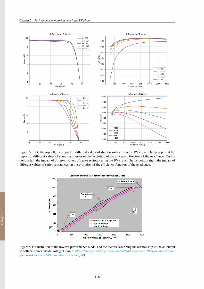
Cha

pter

5

Chapter 5 – Performance monitoring on a large PV plant

Figure 5.3: On the top left, the impact of different values of shunt resistances on the I/V curve. On the top right theimpact of different values of shunt resistances on the evolution of the efficiency function of the irradiance. On thebottom left, the impact of different values of series resistances on the I/V curve. On the bottom right, the impact ofdifferent values of series resistances on the evolution of the efficiency function of the irradiance.

Figure 5.4: Illustration of the inverter performance model and the factors describing the relationship of the ac-outputto both dc-power and dc-voltage (source: https://energy.sandia.gov/wp-content/gallery/uploads/Performance-Model-for-Grid-Connected-Photovoltaic-Inverters.pdf).

116

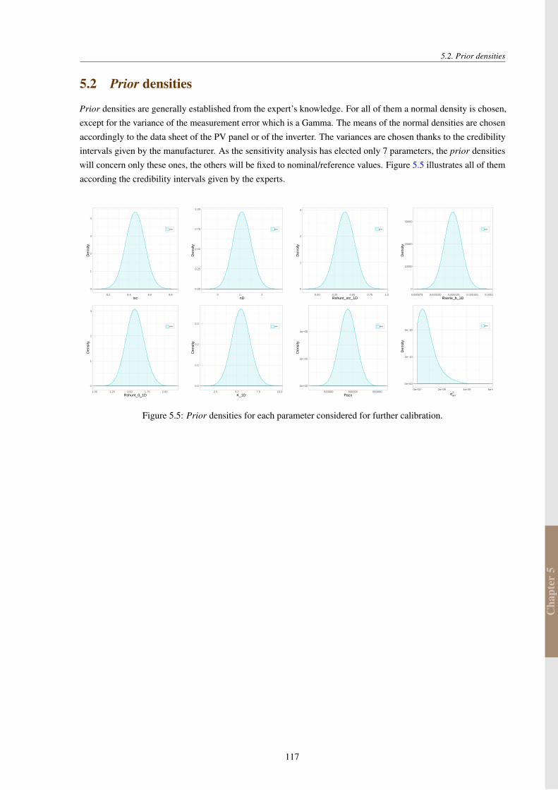
Cha

pter

5

5.2. Prior densities

5.2 Prior densities

Prior densities are generally established from the expert’s knowledge. For all of them a normal density is chosen,except for the variance of the measurement error which is a Gamma. The means of the normal densities are chosenaccordingly to the data sheet of the PV panel or of the inverter. The variances are chosen thanks to the credibilityintervals given by the manufacturer. As the sensitivity analysis has elected only 7 parameters, the prior densitieswill concern only these ones, the others will be fixed to nominal/reference values. Figure 5.5 illustrates all of themaccording the credibility intervals given by the experts.

0

1

2

3

4

8.2 8.4 8.6 8.8Isc

Den

sity

prior

0.00

0.25

0.50

0.75

1.00

0 1 2nD

Den

sity

prior

0

1

2

3

0.00 0.25 0.50 0.75 1.00Rshunt_stc_1D

Den

sity

prior

0

10000

20000

30000

0.000075 0.000100 0.000125 0.000150 0.000175Rserie_b_1D

Den

sity

prior

0

1

2

3

1.00 1.25 1.50 1.75 2.00Rshunt_0_1D

Den

sity

prior

0.0

0.1

0.2

0.3

2.5 5.0 7.5 10.0K_1D

Den

sity

prior

0e+00

2e−05

4e−05

820000 840000 860000Paco

Den

sity

prior

0e+00

2e−10

4e−10

0e+00 2e+09 4e+09 6e+09

σerr2

Den

sity

prior

Figure 5.5: Prior densities for each parameter considered for further calibration.

117

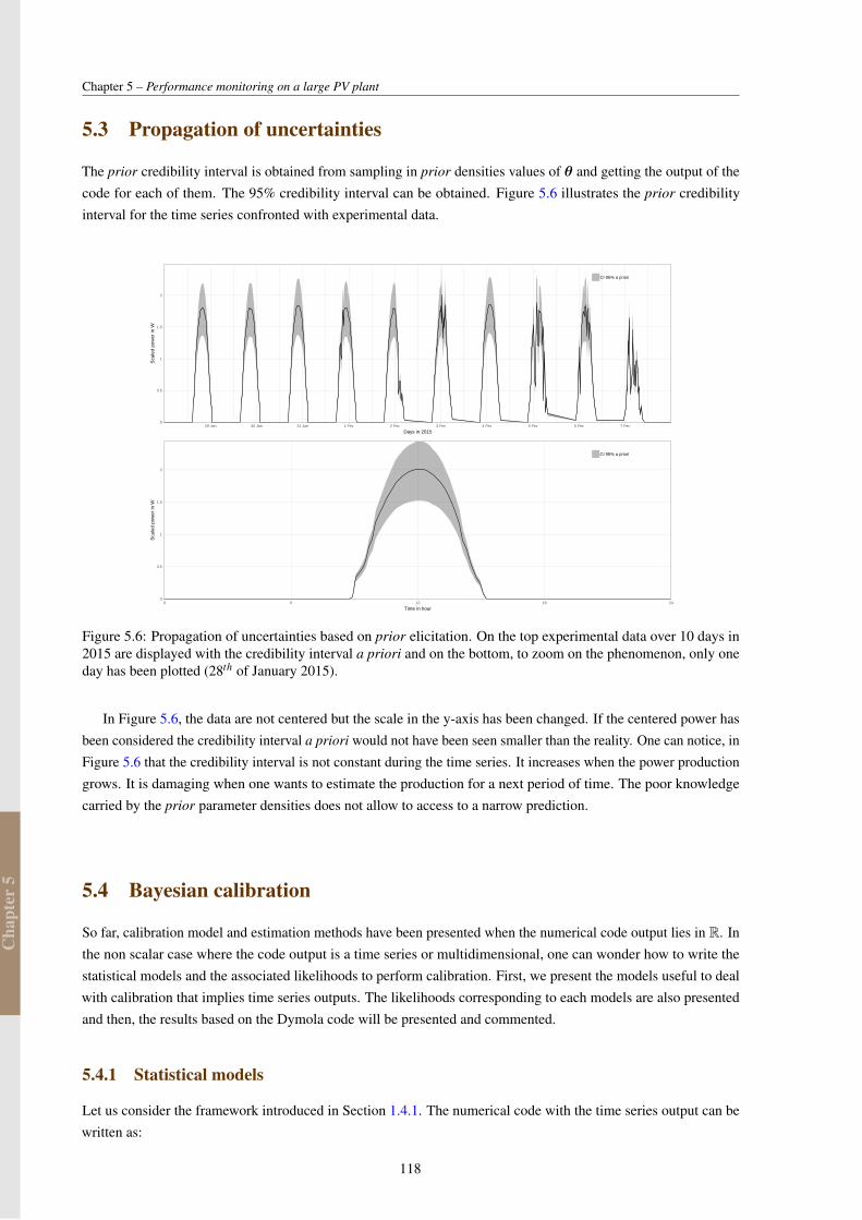
Cha

pter

5

Chapter 5 – Performance monitoring on a large PV plant

5.3 Propagation of uncertainties

The prior credibility interval is obtained from sampling in prior densities values of θ and getting the output of thecode for each of them. The 95% credibility interval can be obtained. Figure 5.6 illustrates the prior credibilityinterval for the time series confronted with experimental data.

0

0.5

1

1.5

2

29 Jan 30 Jan 31 Jan 1 Fev 2 Fev 3 Fev 4 Fev 5 Fev 6 Fev 7 Fev

Days in 2015

Sca

led

pow

er in

W

CI 95% a priori

0

0.5

1

1.5

2

0 6 12 18 24

Time in hour

Sca

led

pow

er in

W

CI 95% a priori

Figure 5.6: Propagation of uncertainties based on prior elicitation. On the top experimental data over 10 days in2015 are displayed with the credibility interval a priori and on the bottom, to zoom on the phenomenon, only oneday has been plotted (28th of January 2015).

In Figure 5.6, the data are not centered but the scale in the y-axis has been changed. If the centered power hasbeen considered the credibility interval a priori would not have been seen smaller than the reality. One can notice, inFigure 5.6 that the credibility interval is not constant during the time series. It increases when the power productiongrows. It is damaging when one wants to estimate the production for a next period of time. The poor knowledgecarried by the prior parameter densities does not allow to access to a narrow prediction.

5.4 Bayesian calibration

So far, calibration model and estimation methods have been presented when the numerical code output lies in R. Inthe non scalar case where the code output is a time series or multidimensional, one can wonder how to write thestatistical models and the associated likelihoods to perform calibration. First, we present the models useful to dealwith calibration that implies time series outputs. The likelihoods corresponding to each models are also presentedand then, the results based on the Dymola code will be presented and commented.

5.4.1 Statistical models

Let us consider the framework introduced in Section 1.4.1. The numerical code with the time series output can bewritten as:

118

Cha

pter

5

5.4. Bayesian calibration

fc : Q→ RT

θ 7→ Y ,(5.1)

where T stands for the number of instantaneous power observed and Q ⊂ Rp. Note that no input variablesX aretaken into account in this formalization since they are implicitly implemented in the Dymola code as mentioned inSection 1.4.4 which is significantly different from the Higdon et al. (2008).

The case of a time consuming code is assumed in this section. To have a surrogate that reproduces a time series,the first idea would be to generate a surrogate for each time step. When T is too high a reduction of dimensionmust be considered. In that respect, a LHS maximin DOE (see Section 2.3) of n points is generated and the timesseries are computed for each configurations of θ. The results are stored in a matrix Y of size n×T . A PCA isperformed on the reduced and centered results matrix Y . It is, then, possible to identify d principal components thatare carrying more than 99% of the total inertia. It means that the sub-space with the d dimensional PCA basis issufficient to represent well enough the simulations. Let us note P the transition matrix from the physical basis tothe PCA basis such as:

P : RT → RT . (5.2)

The matrix P represents the T ×T matrix that allows to get the coordinates of Y on the T PCA axes.

In the space of the PCA, the model M4 (Equation (3.5)) can be projected as:

PYexp = P fc(θ)+P δ +PE. (5.3)

The PCA on simulated data gives the information that all the generated trajectories by the code can be representedat 99% in a d sized orthogonal subspace. It is then possible to identify two subspaces. The first is built with the d

first eigenvectors given by the PCA and the second in the orthogonal subspace generated with the T −d eigenvectorsleft. The PCA tells that P fc(θ) mainly lies in a d-dimension orthogonal subspace. It is then possible to representaccurately the numerical code by using d independent Gaussian processes that emulates the projections of the codeon the d axes of the PCA. The hypothesis made here is to consider that the discrepancy represents everything that isleft over in the T −d dimensional subspace. The statistical model would become:

M ′4 : PYexp = PF

fc1(θ)

...fcd (θ)

+Pδ δ +E = PFF +Pδ δ +E, (5.4)

Model with PCA

where fc1 , . . . , fcd (the components of F ) are equal to P1 fc, . . . ,Pd fc with P1, . . . ,Pd the projections on the d principalcomponents, and E is equal to PE in probability distribution because the matrix P is orthonormal. The PCA isperformed on centered data, so it is possible to formulate the hypothesis that the Gaussian processes on each axiswould be defined as fci(•)∼ G P(0,σ2

pirpi(•,•)). This is a prior belief that is expressed by Higdon et al. (2008)and as code parameters might not have the same impact on the different axis, we rely on anisotropic Gaussianprocesses. The discrepancy represents the rest of the projection of the data on the T − d axes of the PCA andcan be modeled as an independent and identically distributed Gaussian noise which is a random vector definedas δ ∼N (0T−d ,σ

2δ

IT−d). The matrix PF and Pδ are two matrix that are composed of, respectively, the d first

119

Cha

pter

5

Chapter 5 – Performance monitoring on a large PV plant

eigenvectors and the T −d remaining eigenvectors.

If no discrepancy is considered, the statistical model can be simplified as:

M ′2 : PYexp = PFF +E, (5.5)

Model with PCA without discrepancy

5.4.2 Modular estimation and likelihoods

To fulfill a proper modular estimation in the sense of modularization (Liu et al., 2009), the likelihoods have tobe written. The estimation is performed in two steps. On each of the d axis that are supporting the Gaussianprocesses, the partial likelihood can be written from the coordinates of the n points obtained from the DOED usedto perform the PCA. The coordinates on the d axis of the PCA are called Yc1 , . . . ,Ycd . The ith partial likelihood canbe expressed as:

L Mi (Φi;Yci ,D) =

1(2π)n/2|σ2

pirpi(D)|1/2 exp

− 1

2

(Yci

)T(σ2

pirpi(D))−1(Yci

), (5.6)

where σ2pi and rpi are the prior variance of the covariance function and the prior anisotropic correlation function

relative to the ith Gaussian process. The estimation of all the nuisance parameters of each Gaussian process can bedone in a Bayesian framework where prior densities of all the parameters are given and the posterior densities aresampled with MCMC algorithms. It could also be performed using maximum likelihood estimates to get estimatorsof the nuisance parameters.

In a Bayesian framework, the prior densities can be chosen according to Higdon et al. (2008) where they considerσ2

pi as a Gamma distribution, and each ψi j (the correlation lengths in rpi) as a Beta distribution where i would be theith axis and j would be the jth parameter component. Once estimators of the parameters a posteriori, such as the Max-imum A Posteriori (MAP), are found they are plugged into the conditional likelihood. For the following, the methodof using the maximum likelihood estimates to find estimators of each Gaussian processes is picked. Let us, then,consider that the ith Gaussian process conditioned on the DOE is defined as fci(•)|Pi fc(D)∼G P(mi(•),σ2

i ci(•,•)).

In the case where the discrepancy is a white Gaussian noise and independent Gaussian processes are chosen foreach as surrogates on each axis, the full likelihood can be written straightforwardly. If we consider Φ as the set ofthe nuisance parameters for the d surrogates estimators, then the full likelihood of the model M ′

4 is:

L f (PYexp;θ ,σ2err,σ

2δ,Φ) =

1

(2π)d/2Πdi=1

√σ2

err +σ2i (θ)

exp

(−1

2

d

∑i=1

(P TFiYexp−mi(θ))

2

σ2err +σ2

i (θ)

)

1(2π(σ2 +σ2

δ))(T−d)/2 exp

(− 1

2(σ2err +σ2

δ)‖P T

δYexp‖2

).

(5.7)

120

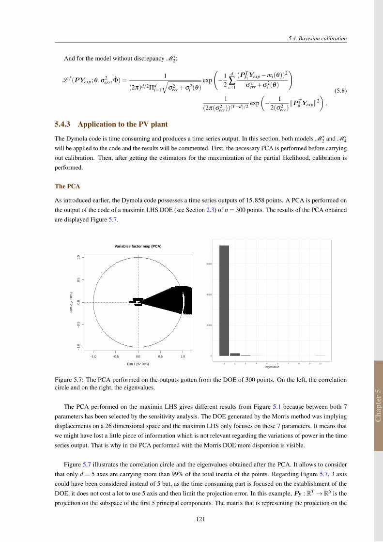
Cha

pter

5

5.4. Bayesian calibration

And for the model without discrepancy M ′2:

L f (PYexp;θ ,σ2err,Φ) =

1

(2π)d/2Πdi=1

√σ2

err +σ2i (θ)

exp

(−1

2

d

∑i=1

(P TFiYexp−mi(θ))

2

σ2err +σ2

i (θ)

)1

(2π(σ2err))

(T−d)/2 exp(− 1

2(σ2err)‖P T

δYexp‖2

).

(5.8)

5.4.3 Application to the PV plant

The Dymola code is time consuming and produces a time series output. In this section, both models M ′2 and M ′

4

will be applied to the code and the results will be commented. First, the necessary PCA is performed before carryingout calibration. Then, after getting the estimators for the maximization of the partial likelihood, calibration isperformed.

The PCA

As introduced earlier, the Dymola code possesses a time series outputs of 15,858 points. A PCA is performed onthe output of the code of a maximin LHS DOE (see Section 2.3) of n = 300 points. The results of the PCA obtainedare displayed Figure 5.7.

−1.0 −0.5 0.0 0.5 1.0

−1.

0−

0.5

0.0

0.5

1.0

Variables factor map (PCA)

Dim 1 (97.20%)

Dim

2 (

2.28

%)

V1V2V3

V4V5

V6V7V8V9V10V11V12V13V14V15V16V17V18V19V20V21V22V23V24V25V26V27V28V29V30V31V32V33V34V35V36V37V38V39V40V41V42

V43

V44 V45V46

V47V48

V49V50V51

V52V53

V54V55V56V57V58

V59V60V61

V62

V63

V64V65V66V67V68V69V70

V71

V72V73

V74

V75V76

V77V78V79

V80V81V82

V83V84V85V86

V87V88V89 V90

V91V92V93

V94

V95

V96V97 V98

V99V100

V101V102V103V104V105V106V107V108V109V110V111V112V113V114V115V116V117V118V119V120V121V122V123V124V125V126V127V128V129V130V131V132V133V134V135V136V137V138

V139

V140

V141V142

V143V144

V145V146V147

V148

V149V150

V151V152

V153

V154V155 V156

V157V158V159V160

V161V162V163V164V165

V166

V167V168V169

V170V171V172 V173V174

V175V176

V177V178

V179V180V181 V182

V183V184V185V186

V187

V188V189V190 V191

V192

V193V194

V195V196

V197V198V199V200V201V202V203V204V205V206V207V208V209

V210V211V212V213V214V215V216

V217V218V219V220V221V222V223V224V225V226V227V228V229V230V231V232V233V234V235

V236

V237V238V239V240V241

V242V243V244V245V246

V247V248

V249

V250

V251V252V253

V254

V255V256

V257

V258V259

V260V261V262 V263

V264V265V266V267V268

V269

V270

V271V272

V273

V274

V275V276V277V278

V279

V280V281

V282

V283V284V285V286V287V288

V289

V290V291

V292

V293V294V295V296V297V298V299V300V301V302V303V304V305V306V307V308

V309V310V311V312

V313V314V315

V316V317V318

V319V320V321V322V323V324V325V326V327V328V329V330

V331

V332V333

V334V335

V336V337

V338 V339V340

V341V342

V343V344V345V346V347

V348

V349

V350V351V352

V353

V354

V355V356

V357V358V359V360V361

V362V363

V364V365V366

V367V368V369

V370V371 V372V373

V374

V375V376V377

V378V379

V380V381

V382

V383V384V385

V386V387

V388

V389V390V391V392V393V394V395V396V397V398V399V400V401V402V403V404V405V406V407V408V409V410V411V412V413V414V415V416V417V418V419V420V421V422V423V424V425V426

V427V428V429V430V431V432V433V434V435V436V437V438V439V440V441V442V443V444V445V446V447V448V449V450V451V452V453V454V455V456V457V458V459V460V461V462V463V464V465V466V467V468V469V470V471V472V473V474V475V476V477V478V479V480V481V482V483V484

V485V486V487V488V489V490V491V492

V493V494V495V496V497V498V499V500V501V502V503V504V505V506V507V508V509V510V511V512V513V514V515V516V517V518V519V520V521V522V523

V524V525V526V527V528V529V530V531V532V533V534V535V536V537V538V539V540V541V542V543V544V545V546V547V548V549V550V551V552V553V554V555V556V557V558V559V560V561V562V563V564V565V566V567V568V569V570V571V572V573V574V575V576V577V578V579V580V581V582V583

V584

V585V586V587V588V589V590V591V592V593V594

V595V596V597V598

V599V600V601V602V603

V604V605V606V607

V608V609V610V611V612

V613V614V615V616V617V618

V619

V620V621V622V623V624V625V626V627V628V629V630V631V632V633V634V635V636V637V638V639V640V641V642V643V644V645V646V647V648V649V650V651V652V653V654V655V656V657V658V659V660V661V662V663V664V665V666V667V668V669V670V671V672V673V674V675V676V677

V678V679V680V681V682V683V684V685V686V687V688V689V690V691V692V693

V694V695V696V697V698V699V700V701V702V703V704V705V706V707V708V709V710V711

V712V713

V714V715V716V717V718V719V720V721V722V723V724V725V726V727V728V729V730V731V732V733V734V735V736V737V738V739V740V741V742V743V744V745V746V747V748V749V750V751V752V753V754V755V756V757V758V759V760V761V762V763V764V765V766V767V768V769V770V771V772V773

V774V775V776

V777V778V779V780V781V782V783V784V785V786V787V788V789V790V791V792V793V794V795V796V797V798V799V800V801V802V803V804V805V806V807

V808V809

V810V811V812V813V814V815V816V817V818V819V820V821V822V823V824V825V826V827V828V829V830V831V832V833V834V835V836V837V838V839V840V841V842V843V844V845V846V847V848V849V850V851V852V853V854V855V856V857V858V859V860V861V862V863V864V865V866V867V868

V869V870V871V872V873V874V875V876V877V878

V879V880V881V882V883V884V885V886V887V888V889V890V891

V892V893V894V895V896V897V898V899V900V901V902

V903V904

V905V906V907V908V909V910V911V912V913V914V915V916V917V918V919V920V921V922V923V924V925V926V927V928V929V930V931V932V933V934V935V936V937V938V939V940V941V942V943V944V945V946V947V948V949V950V951V952V953V954V955V956V957V958V959V960V961V962V963V964

V965V966V967V968V969V970

V971V972

V973V974V975V976V977

V978

V979

V980V981V982V983V984V985

V986

V987V988

V989

V990V991

V992V993V994

V995V996V997V998V999V1000V1001V1002

V1003

V1004V1005V1006V1007V1008V1009V1010V1011V1012V1013V1014V1015V1016V1017V1018V1019V1020V1021V1022V1023V1024V1025V1026V1027V1028V1029V1030V1031V1032V1033V1034V1035V1036V1037V1038V1039V1040V1041V1042V1043V1044V1045V1046V1047V1048V1049V1050V1051V1052V1053V1054V1055V1056V1057V1058V1059V1060

V1061V1062V1063V1064V1065V1066V1067V1068V1069V1070V1071V1072V1073V1074V1075V1076V1077V1078V1079V1080V1081V1082V1083V1084V1085V1086V1087V1088V1089V1090V1091V1092V1093V1094V1095V1096V1097V1098

V1099

V1100V1101V1102V1103V1104V1105V1106V1107V1108V1109V1110V1111V1112V1113V1114V1115V1116V1117V1118V1119V1120V1121V1122V1123V1124V1125V1126V1127V1128V1129V1130V1131V1132V1133V1134V1135V1136V1137V1138V1139V1140V1141V1142V1143V1144V1145V1146V1147V1148V1149V1150V1151V1152V1153V1154V1155V1156

V1157V1158V1159V1160V1161V1162V1163V1164V1165V1166V1167V1168V1169V1170V1171V1172V1173V1174V1175V1176V1177V1178V1179V1180V1181V1182V1183V1184V1185V1186V1187V1188V1189V1190V1191V1192V1193V1194

V1195

V1196V1197V1198V1199V1200V1201V1202V1203V1204V1205V1206V1207V1208V1209V1210V1211V1212V1213V1214V1215V1216V1217V1218V1219V1220V1221V1222V1223V1224V1225V1226V1227V1228V1229V1230V1231V1232V1233V1234V1235V1236V1237V1238V1239V1240V1241V1242V1243V1244V1245V1246V1247V1248V1249V1250V1251V1252

V1253V1254V1255V1256V1257V1258V1259V1260V1261V1262V1263V1264V1265V1266V1267V1268

V1269V1270

V1271V1272V1273V1274V1275V1276V1277V1278V1279V1280V1281V1282V1283V1284V1285V1286V1287

V1288V1289V1290V1291

V1292V1293V1294V1295V1296V1297V1298V1299V1300V1301V1302V1303V1304V1305V1306V1307V1308V1309V1310V1311V1312V1313V1314V1315V1316V1317V1318V1319V1320V1321V1322V1323V1324V1325V1326V1327V1328V1329V1330V1331V1332V1333V1334V1335V1336V1337V1338V1339V1340V1341V1342V1343V1344V1345V1346V1347V1348

V1349V1350V1351V1352V1353V1354V1355V1356V1357V1358V1359

V1360

V1361V1362V1363

V1364V1365V1366

V1367V1368V1369V1370V1371V1372V1373

V1374V1375V1376V1377V1378V1379V1380V1381

V1382V1383V1384

V1385V1386V1387V1388V1389V1390V1391V1392V1393V1394V1395V1396V1397V1398V1399V1400V1401V1402V1403V1404V1405V1406V1407V1408V1409V1410V1411V1412V1413V1414V1415V1416V1417V1418V1419V1420V1421V1422V1423V1424V1425V1426V1427V1428V1429V1430V1431V1432V1433V1434V1435V1436V1437V1438V1439V1440V1441V1442V1443V1444

V1445V1446V1447V1448V1449V1450V1451V1452V1453V1454V1455V1456V1457V1458V1459V1460V1461V1462V1463V1464

V1465V1466V1467V1468V1469

V1470

V1471V1472

V1473V1474

V1475V1476V1477V1478V1479V1480V1481V1482V1483

V1484

V1485V1486V1487V1488V1489V1490V1491V1492V1493V1494V1495V1496V1497V1498V1499V1500V1501V1502V1503V1504V1505V1506V1507V1508V1509V1510V1511V1512V1513V1514V1515V1516V1517V1518V1519V1520V1521V1522V1523V1524V1525V1526V1527V1528V1529V1530V1531V1532V1533V1534V1535V1536V1537V1538V1539V1540

V1541V1542V1543V1544V1545V1546V1547V1548V1549V1550V1551V1552

V1553V1554

V1555V1556V1557V1558

V1559

V1560V1561V1562V1563V1564V1565V1566V1567V1568V1569V1570V1571V1572V1573V1574V1575V1576V1577V1578V1579

V1580

V1581V1582V1583V1584V1585V1586V1587V1588V1589V1590V1591V1592V1593V1594V1595V1596V1597V1598V1599V1600V1601V1602V1603V1604V1605V1606V1607V1608V1609V1610V1611V1612V1613V1614V1615V1616V1617V1618V1619V1620V1621V1622V1623V1624V1625V1626V1627V1628V1629V1630V1631V1632V1633V1634V1635V1636

V1637V1638V1639V1640V1641V1642V1643V1644V1645V1646V1647V1648V1649V1650V1651V1652V1653V1654V1655V1656V1657V1658V1659V1660V1661V1662V1663V1664V1665V1666V1667V1668V1669V1670V1671V1672V1673V1674

V1675V1676

V1677V1678V1679V1680V1681V1682V1683V1684V1685V1686V1687V1688V1689V1690V1691V1692V1693V1694V1695V1696V1697V1698V1699V1700V1701V1702V1703V1704V1705V1706V1707V1708V1709V1710V1711V1712V1713V1714V1715V1716V1717V1718V1719V1720V1721V1722V1723V1724V1725V1726V1727V1728V1729V1730V1731V1732

V1733V1734V1735V1736V1737V1738V1739V1740V1741V1742V1743V1744

V1745V1746V1747V1748V1749V1750V1751V1752V1753V1754

V1755V1756V1757

V1758

V1759V1760V1761V1762V1763V1764V1765V1766V1767V1768V1769V1770V1771

V1772

V1773V1774V1775V1776V1777V1778V1779V1780V1781V1782V1783V1784V1785V1786V1787V1788V1789V1790V1791V1792V1793V1794V1795V1796V1797V1798V1799V1800V1801V1802V1803V1804V1805V1806V1807V1808V1809V1810V1811V1812V1813V1814V1815V1816V1817V1818V1819V1820V1821V1822V1823V1824V1825V1826V1827V1828

V1829

V1830V1831V1832V1833V1834V1835V1836V1837V1838V1839V1840V1841V1842V1843V1844V1845V1846V1847V1848V1849V1850V1851V1852V1853V1854V1855V1856V1857V1858V1859V1860V1861V1862V1863V1864V1865V1866V1867

V1868

V1869V1870V1871V1872V1873V1874V1875V1876V1877V1878V1879V1880V1881V1882V1883V1884V1885V1886V1887V1888V1889V1890V1891V1892V1893V1894V1895V1896V1897V1898V1899V1900V1901V1902V1903V1904V1905V1906V1907V1908V1909V1910V1911V1912V1913V1914V1915V1916V1917V1918V1919V1920V1921V1922V1923V1924V1925V1926V1927V1928V1929V1930V1931V1932V1933V1934V1935V1936V1937V1938V1939V1940V1941V1942V1943V1944V1945V1946V1947V1948V1949V1950V1951V1952V1953V1954V1955V1956V1957V1958V1959V1960V1961V1962V1963

V1964V1965V1966V1967V1968V1969V1970V1971V1972V1973V1974V1975V1976V1977V1978V1979V1980V1981V1982V1983V1984V1985V1986V1987V1988V1989V1990V1991V1992V1993V1994V1995V1996V1997V1998V1999V2000V2001V2002V2003V2004V2005V2006V2007V2008V2009V2010V2011V2012V2013V2014V2015V2016V2017V2018V2019V2020V2021

V2022V2023V2024V2025V2026V2027V2028V2029V2030V2031V2032V2033V2034V2035V2036V2037V2038V2039V2040V2041V2042V2043V2044V2045V2046V2047V2048V2049V2050V2051V2052V2053V2054V2055V2056V2057V2058V2059

V2060V2061V2062V2063V2064V2065V2066V2067V2068V2069V2070V2071V2072V2073V2074V2075V2076V2077V2078V2079V2080V2081V2082V2083V2084V2085V2086V2087V2088V2089V2090V2091V2092V2093V2094V2095V2096V2097V2098V2099V2100V2101V2102V2103V2104V2105V2106V2107V2108V2109V2110V2111V2112V2113V2114V2115V2116V2117V2118V2119V2120V2121V2122V2123V2124V2125V2126V2127V2128V2129V2130V2131V2132V2133V2134V2135V2136V2137V2138V2139V2140V2141V2142V2143V2144V2145V2146V2147V2148V2149V2150V2151V2152V2153V2154V2155V2156

V2157V2158V2159V2160V2161V2162V2163V2164V2165V2166V2167V2168V2169V2170V2171V2172V2173V2174V2175V2176V2177V2178V2179V2180V2181V2182V2183V2184V2185V2186V2187V2188V2189V2190V2191V2192V2193V2194V2195V2196V2197V2198V2199V2200V2201V2202V2203V2204V2205V2206V2207V2208V2209V2210V2211V2212

V2213

V2214V2215V2216V2217V2218V2219V2220V2221V2222V2223V2224V2225V2226V2227V2228V2229V2230V2231V2232V2233V2234V2235V2236V2237V2238V2239V2240V2241V2242V2243V2244V2245V2246V2247V2248V2249V2250V2251

V2252

V2253V2254V2255V2256V2257V2258V2259V2260V2261V2262V2263V2264V2265V2266V2267V2268V2269V2270V2271V2272V2273V2274V2275V2276V2277V2278V2279V2280V2281V2282V2283V2284V2285V2286V2287V2288V2289V2290V2291V2292V2293V2294V2295V2296V2297V2298V2299V2300V2301V2302V2303V2304V2305V2306V2307V2308

V2309V2310V2311V2312V2313V2314V2315V2316V2317V2318V2319V2320V2321V2322V2323V2324V2325V2326V2327V2328V2329V2330V2331V2332V2333V2334V2335V2336V2337V2338V2339V2340V2341V2342V2343V2344V2345V2346V2347V2348

V2349V2350V2351V2352V2353V2354V2355V2356V2357V2358V2359V2360V2361V2362V2363V2364V2365V2366V2367V2368V2369V2370V2371V2372V2373V2374V2375V2376V2377V2378V2379V2380V2381V2382V2383V2384V2385V2386V2387V2388V2389V2390V2391V2392V2393V2394V2395V2396V2397V2398V2399V2400V2401V2402V2403V2404

V2405V2406V2407V2408V2409V2410V2411V2412V2413V2414V2415V2416V2417

V2418V2419V2420V2421V2422V2423V2424V2425V2426V2427V2428V2429V2430V2431V2432V2433V2434V2435V2436V2437V2438V2439V2440V2441V2442V2443V2444

V2445V2446V2447V2448V2449V2450V2451V2452V2453V2454V2455V2456V2457V2458V2459V2460V2461V2462V2463V2464V2465V2466V2467V2468V2469V2470V2471V2472V2473V2474V2475V2476V2477V2478V2479V2480V2481V2482V2483V2484V2485V2486V2487V2488V2489V2490V2491V2492V2493V2494V2495V2496V2497V2498V2499V2500

V2501V2502V2503V2504V2505V2506V2507V2508V2509V2510V2511V2512V2513V2514V2515V2516V2517V2518V2519V2520V2521V2522V2523V2524V2525V2526V2527V2528V2529V2530V2531V2532V2533V2534V2535V2536V2537V2538V2539V2540

V2541V2542V2543V2544V2545V2546V2547V2548V2549V2550V2551V2552V2553V2554V2555V2556V2557V2558V2559V2560V2561V2562V2563V2564V2565V2566V2567V2568V2569V2570V2571V2572V2573V2574V2575V2576V2577V2578V2579V2580V2581V2582V2583V2584V2585V2586V2587V2588V2589V2590V2591V2592V2593V2594V2595V2596

V2597

V2598V2599V2600V2601V2602V2603V2604V2605V2606V2607V2608V2609V2610V2611

V2612V2613

V2614V2615

V2616V2617V2618

V2619V2620V2621V2622V2623V2624V2625

V2626V2627V2628V2629V2630V2631V2632V2633V2634V2635

V2636

V2637V2638V2639V2640V2641V2642V2643V2644V2645V2646V2647V2648V2649V2650V2651V2652V2653V2654V2655V2656V2657V2658V2659V2660V2661V2662V2663V2664V2665V2666V2667V2668V2669V2670V2671V2672V2673V2674V2675V2676V2677V2678V2679V2680V2681V2682V2683V2684V2685V2686V2687V2688V2689V2690V2691V2692

V2693V2694V2695V2696V2697V2698V2699V2700V2701V2702V2703V2704V2705V2706V2707V2708V2709V2710V2711V2712V2713V2714V2715V2716V2717V2718V2719V2720V2721V2722V2723V2724V2725V2726V2727V2728V2729V2730V2731

V2732

V2733V2734V2735V2736V2737V2738V2739V2740V2741V2742V2743V2744V2745V2746V2747V2748V2749V2750V2751V2752V2753V2754V2755V2756V2757V2758V2759V2760V2761V2762V2763V2764V2765V2766V2767V2768V2769V2770V2771V2772V2773V2774V2775V2776V2777V2778V2779V2780V2781V2782V2783V2784V2785V2786V2787V2788

V2789

V2790V2791V2792V2793V2794V2795V2796V2797V2798V2799V2800V2801V2802V2803V2804V2805V2806V2807V2808V2809V2810V2811V2812V2813V2814V2815V2816V2817V2818V2819V2820V2821V2822V2823V2824V2825V2826V2827V2828

V2829V2830V2831V2832V2833V2834V2835V2836V2837V2838V2839V2840V2841V2842V2843V2844V2845V2846V2847V2848V2849V2850V2851V2852V2853V2854V2855V2856V2857V2858V2859V2860V2861V2862V2863V2864V2865V2866V2867V2868V2869V2870V2871V2872V2873V2874V2875V2876V2877V2878V2879V2880V2881V2882V2883V2884

V2885

V2886V2887V2888V2889V2890V2891V2892V2893V2894V2895V2896V2897V2898V2899V2900V2901V2902V2903V2904V2905V2906V2907V2908V2909V2910V2911V2912V2913V2914V2915V2916V2917V2918V2919V2920V2921V2922V2923V2924

V2925V2926V2927V2928V2929V2930V2931V2932V2933V2934V2935V2936V2937V2938V2939V2940V2941V2942V2943V2944V2945V2946V2947V2948V2949V2950V2951V2952V2953V2954V2955V2956V2957V2958V2959V2960V2961V2962V2963V2964V2965V2966V2967V2968V2969V2970V2971V2972V2973V2974V2975V2976V2977V2978V2979V2980

V2981

V2982V2983V2984V2985V2986V2987V2988V2989V2990V2991V2992V2993V2994V2995V2996V2997V2998V2999V3000V3001V3002V3003V3004V3005V3006V3007V3008V3009V3010V3011V3012V3013V3014V3015V3016V3017V3018V3019V3020

V3021V3022V3023V3024V3025V3026V3027V3028V3029V3030V3031V3032V3033V3034V3035V3036V3037V3038V3039V3040V3041V3042V3043V3044V3045V3046V3047V3048V3049V3050V3051V3052V3053V3054V3055V3056V3057V3058V3059V3060V3061V3062V3063V3064V3065V3066V3067V3068V3069V3070V3071V3072V3073V3074V3075V3076

V3077

V3078V3079V3080V3081V3082V3083V3084V3085V3086V3087V3088V3089V3090V3091V3092V3093V3094V3095V3096V3097V3098V3099V3100V3101V3102V3103V3104V3105V3106V3107V3108V3109V3110V3111V3112V3113V3114V3115

V3116

V3117V3118V3119V3120V3121V3122V3123V3124V3125V3126V3127V3128V3129V3130V3131V3132V3133V3134V3135V3136V3137V3138V3139V3140V3141V3142V3143V3144V3145V3146V3147V3148V3149V3150V3151V3152V3153V3154V3155V3156V3157V3158V3159V3160V3161V3162V3163V3164V3165V3166V3167V3168V3169V3170V3171V3172

V3173

V3174V3175V3176V3177V3178V3179V3180V3181V3182V3183V3184V3185V3186V3187V3188V3189V3190V3191V3192V3193V3194V3195V3196V3197V3198V3199V3200

V3201V3202V3203V3204V3205V3206V3207V3208V3209V3210V3211V3212

V3213

V3214V3215V3216V3217V3218V3219V3220V3221V3222V3223V3224V3225V3226V3227V3228V3229V3230V3231V3232V3233V3234V3235V3236V3237V3238V3239V3240V3241V3242V3243V3244V3245V3246V3247V3248V3249V3250V3251V3252V3253V3254V3255V3256V3257V3258V3259V3260V3261V3262V3263V3264V3265V3266V3267V3268

V3269V3270V3271V3272V3273V3274V3275V3276V3277V3278V3279V3280V3281V3282V3283V3284V3285V3286V3287V3288V3289

V3290V3291V3292V3293V3294V3295V3296V3297V3298V3299V3300V3301V3302V3303V3304V3305V3306V3307V3308

V3309

V3310V3311V3312V3313V3314V3315V3316V3317V3318V3319V3320V3321V3322V3323V3324V3325V3326V3327V3328V3329V3330V3331V3332V3333V3334V3335V3336V3337V3338V3339V3340V3341V3342V3343V3344V3345V3346V3347V3348V3349V3350V3351V3352V3353V3354V3355V3356V3357V3358V3359V3360V3361V3362V3363V3364

V3365

V3366V3367V3368V3369V3370V3371V3372V3373V3374V3375V3376V3377V3378V3379V3380V3381V3382V3383V3384V3385V3386V3387V3388V3389V3390V3391V3392V3393V3394V3395V3396V3397V3398V3399V3400V3401V3402V3403V3404

V3405

V3406V3407V3408V3409V3410V3411V3412V3413V3414V3415V3416V3417V3418V3419V3420V3421V3422V3423V3424V3425V3426V3427V3428V3429V3430V3431V3432V3433V3434V3435V3436V3437V3438V3439V3440V3441V3442V3443V3444V3445V3446V3447V3448V3449V3450V3451V3452V3453V3454V3455V3456V3457V3458V3459V3460

V3461V3462V3463V3464V3465V3466V3467V3468V3469V3470V3471V3472

V3473V3474V3475V3476

V3477V3478V3479V3480V3481V3482

V3483V3484V3485V3486V3487V3488V3489V3490

V3491

V3492

V3493V3494

V3495V3496V3497V3498V3499V3500

V3501

V3502V3503V3504V3505V3506V3507V3508V3509V3510V3511V3512V3513V3514V3515V3516V3517V3518V3519V3520V3521V3522V3523V3524V3525V3526V3527V3528V3529V3530V3531V3532V3533V3534V3535V3536V3537V3538V3539V3540V3541V3542V3543V3544V3545V3546V3547V3548V3549V3550V3551V3552V3553V3554V3555

V3556V3557V3558V3559V3560V3561V3562V3563V3564

V3565V3566

V3567V3568V3569V3570V3571V3572V3573V3574V3575V3576V3577

V3578V3579V3580V3581V3582V3583V3584V3585V3586V3587V3588V3589V3590V3591V3592V3593V3594V3595V3596

V3597

V3598V3599V3600V3601V3602V3603V3604V3605V3606V3607V3608V3609V3610V3611V3612V3613V3614V3615V3616V3617V3618V3619V3620V3621V3622V3623V3624V3625V3626V3627V3628V3629V3630V3631V3632V3633V3634V3635V3636V3637V3638V3639V3640V3641V3642V3643V3644V3645V3646V3647V3648V3649V3650V3651

V3652V3653V3654V3655V3656V3657V3658V3659V3660

V3661V3662

V3663

V3664V3665V3666V3667V3668V3669

V3670V3671V3672V3673V3674V3675V3676V3677V3678V3679V3680V3681V3682V3683V3684V3685V3686V3687V3688V3689V3690V3691V3692

V3693V3694V3695V3696V3697V3698V3699V3700V3701V3702V3703V3704V3705V3706V3707V3708V3709V3710V3711V3712V3713V3714V3715V3716V3717V3718V3719V3720V3721V3722V3723V3724V3725V3726V3727V3728V3729V3730V3731V3732V3733V3734V3735V3736V3737V3738V3739V3740V3741V3742V3743V3744V3745V3746V3747V3748

V3749V3750V3751V3752V3753V3754V3755V3756V3757V3758V3759V3760V3761V3762V3763V3764V3765V3766V3767V3768V3769V3770V3771V3772V3773V3774V3775V3776V3777V3778V3779V3780V3781V3782V3783V3784V3785V3786V3787V3788

V3789

V3790V3791V3792V3793V3794V3795V3796V3797V3798V3799V3800V3801V3802V3803V3804V3805V3806V3807V3808V3809V3810V3811V3812V3813V3814V3815V3816V3817V3818V3819V3820V3821V3822V3823V3824V3825V3826V3827V3828V3829V3830V3831V3832V3833V3834V3835V3836V3837V3838V3839V3840V3841V3842V3843

V3844V3845V3846V3847V3848V3849V3850V3851V3852V3853V3854V3855V3856V3857V3858V3859V3860V3861V3862V3863V3864V3865V3866V3867V3868V3869V3870V3871V3872V3873V3874V3875V3876V3877V3878V3879V3880V3881V3882V3883V3884V3885

V3886V3887V3888V3889V3890V3891V3892V3893V3894V3895V3896V3897V3898V3899V3900V3901V3902V3903V3904V3905V3906V3907V3908V3909V3910V3911V3912V3913V3914V3915V3916V3917V3918V3919V3920V3921V3922V3923V3924V3925V3926V3927V3928V3929V3930V3931V3932V3933V3934V3935V3936V3937V3938V3939

V3940V3941V3942V3943V3944V3945V3946V3947V3948V3949V3950V3951V3952V3953V3954V3955V3956V3957V3958V3959V3960V3961V3962V3963V3964V3965V3966V3967V3968V3969V3970V3971V3972V3973V3974V3975V3976V3977V3978V3979V3980V3981

V3982V3983V3984V3985V3986V3987V3988V3989V3990V3991V3992V3993V3994V3995V3996V3997V3998V3999V4000V4001V4002V4003V4004V4005V4006V4007V4008V4009V4010V4011V4012V4013V4014V4015V4016V4017V4018V4019V4020V4021V4022V4023V4024V4025V4026V4027V4028V4029V4030V4031V4032V4033V4034V4035

V4036V4037V4038V4039V4040V4041V4042V4043V4044V4045V4046V4047V4048V4049V4050V4051V4052V4053V4054V4055V4056V4057V4058V4059V4060

V4061V4062V4063V4064V4065V4066V4067V4068V4069V4070V4071V4072V4073V4074V4075V4076

V4077

V4078V4079V4080V4081V4082V4083V4084V4085V4086V4087V4088V4089V4090V4091V4092V4093V4094V4095V4096V4097V4098V4099V4100V4101V4102V4103V4104V4105V4106V4107V4108V4109V4110V4111V4112V4113V4114V4115V4116V4117V4118V4119V4120V4121V4122V4123V4124V4125V4126V4127V4128V4129V4130V4131

V4132

V4133V4134V4135V4136V4137V4138V4139V4140V4141V4142V4143V4144V4145V4146V4147

V4148V4149V4150V4151V4152V4153V4154V4155V4156V4157V4158V4159

V4160V4161V4162

V4163V4164V4165V4166

V4167V4168V4169V4170V4171V4172V4173

V4174V4175V4176V4177V4178V4179V4180V4181V4182V4183V4184V4185V4186V4187V4188V4189V4190V4191V4192V4193V4194V4195V4196V4197V4198V4199V4200V4201V4202V4203V4204V4205V4206V4207V4208V4209V4210V4211V4212V4213V4214V4215V4216V4217V4218V4219V4220V4221V4222V4223V4224V4225V4226V4227

V4228

V4229V4230V4231V4232V4233V4234V4235V4236V4237V4238V4239V4240V4241V4242V4243V4244V4245V4246V4247V4248V4249V4250V4251

V4252V4253

V4254V4255V4256V4257V4258V4259V4260V4261V4262V4263V4264V4265V4266V4267V4268

V4269

V4270V4271V4272V4273V4274V4275V4276V4277V4278V4279V4280V4281V4282V4283V4284V4285V4286V4287V4288V4289V4290V4291V4292V4293V4294V4295V4296V4297V4298V4299V4300V4301V4302V4303V4304V4305V4306V4307V4308V4309V4310V4311V4312V4313V4314V4315V4316V4317V4318V4319V4320V4321V4322V4323V4324

V4325V4326V4327V4328V4329V4330V4331V4332V4333V4334V4335V4336V4337V4338V4339V4340V4341V4342V4343V4344V4345V4346V4347V4348V4349V4350V4351V4352V4353V4354V4355V4356V4357V4358V4359V4360V4361V4362V4363V4364

V4365V4366V4367V4368V4369V4370V4371V4372V4373V4374V4375V4376V4377V4378V4379V4380V4381V4382V4383V4384V4385V4386V4387V4388V4389V4390V4391V4392V4393V4394V4395V4396V4397V4398V4399V4400V4401V4402V4403V4404V4405V4406V4407V4408V4409V4410V4411V4412V4413V4414V4415V4416V4417V4418V4419

V4420V4421V4422V4423V4424V4425V4426V4427V4428V4429V4430V4431V4432V4433V4434

V4435V4436V4437V4438

V4439V4440

V4441

V4442V4443V4444V4445

V4446

V4447V4448V4449V4450V4451V4452V4453V4454V4455V4456V4457V4458V4459V4460

V4461

V4462V4463V4464V4465V4466V4467V4468V4469V4470V4471V4472V4473V4474V4475V4476V4477V4478V4479V4480V4481V4482V4483V4484V4485V4486V4487V4488V4489V4490V4491V4492V4493V4494V4495V4496V4497V4498V4499V4500V4501V4502V4503V4504V4505V4506V4507V4508V4509V4510V4511V4512V4513V4514V4515

V4516V4517V4518V4519V4520V4521V4522V4523V4524V4525V4526V4527V4528V4529V4530V4531V4532

V4533

V4534V4535V4536V4537V4538V4539V4540

V4541V4542

V4543

V4544V4545V4546

V4547V4548V4549V4550V4551V4552V4553V4554V4555V4556V4557

V4558

V4559V4560V4561V4562V4563V4564V4565V4566V4567V4568V4569V4570V4571V4572V4573V4574V4575V4576V4577V4578V4579V4580V4581V4582V4583V4584V4585V4586V4587V4588V4589V4590V4591V4592V4593V4594V4595V4596V4597V4598V4599V4600V4601V4602V4603V4604V4605V4606V4607V4608V4609V4610V4611

V4612V4613V4614V4615V4616V4617V4618V4619

V4620V4621V4622V4623V4624V4625V4626V4627

V4628V4629

V4630V4631V4632V4633V4634V4635V4636V4637V4638

V4639V4640V4641V4642V4643V4644V4645V4646V4647V4648V4649V4650V4651V4652V4653

V4654

V4655V4656V4657V4658V4659V4660V4661V4662V4663V4664V4665V4666V4667V4668V4669V4670V4671V4672V4673V4674V4675V4676V4677V4678V4679V4680V4681V4682V4683V4684V4685V4686V4687V4688V4689V4690V4691V4692V4693V4694V4695V4696V4697V4698V4699V4700V4701V4702V4703V4704V4705V4706V4707

V4708V4709V4710V4711V4712V4713V4714V4715V4716V4717V4718V4719V4720V4721V4722V4723V4724V4725V4726V4727V4728V4729V4730V4731

V4732V4733V4734V4735

V4736V4737

V4738

V4739V4740V4741V4742V4743

V4744

V4745V4746

V4747V4748

V4749V4750V4751V4752V4753V4754V4755V4756V4757V4758V4759V4760V4761V4762V4763V4764V4765V4766V4767V4768V4769V4770V4771V4772V4773V4774V4775V4776V4777V4778V4779V4780V4781V4782V4783V4784V4785V4786V4787V4788V4789V4790V4791V4792V4793V4794V4795V4796V4797V4798V4799V4800V4801V4802V4803

V4804V4805V4806V4807

V4808

V4809V4810V4811V4812V4813V4814V4815V4816V4817V4818V4819V4820V4821V4822V4823

V4824V4825

V4826V4827

V4828V4829V4830

V4831V4832

V4833V4834V4835V4836V4837V4838

V4839

V4840V4841V4842V4843V4844V4845

V4846

V4847V4848V4849V4850V4851V4852V4853V4854V4855V4856V4857V4858V4859V4860V4861V4862V4863V4864V4865V4866V4867V4868V4869V4870V4871V4872V4873V4874V4875V4876V4877V4878V4879V4880V4881V4882V4883V4884V4885V4886V4887V4888V4889V4890V4891V4892V4893V4894V4895V4896V4897V4898

V4899V4900V4901V4902V4903V4904V4905V4906V4907V4908V4909

V4910

V4911

V4912V4913V4914V4915

V4916

V4917V4918

V4919V4920

V4921V4922V4923V4924

V4925

V4926

V4927V4928V4929V4930V4931V4932V4933

V4934V4935V4936V4937V4938V4939V4940V4941

V4942

V4943V4944V4945V4946V4947V4948V4949V4950V4951V4952V4953V4954V4955V4956V4957V4958V4959V4960V4961V4962V4963V4964V4965V4966V4967V4968V4969V4970V4971V4972V4973V4974V4975V4976V4977V4978V4979V4980V4981V4982V4983V4984V4985V4986V4987V4988V4989V4990V4991V4992V4993V4994V4995

V4996V4997V4998V4999V5000V5001V5002V5003V5004V5005V5006V5007V5008V5009V5010V5011V5012V5013V5014V5015V5016V5017V5018V5019V5020V5021

V5022V5023V5024V5025V5026V5027V5028

V5029V5030V5031V5032V5033V5034V5035V5036V5037

V5038

V5039V5040V5041V5042V5043V5044V5045V5046V5047V5048V5049V5050V5051V5052V5053V5054V5055V5056V5057V5058V5059V5060V5061V5062V5063V5064V5065V5066V5067V5068V5069V5070V5071V5072V5073V5074V5075V5076V5077V5078V5079V5080V5081V5082V5083V5084V5085V5086V5087V5088V5089V5090

V5091V5092V5093V5094V5095V5096V5097V5098V5099V5100V5101V5102V5103V5104V5105V5106V5107V5108V5109V5110V5111V5112V5113V5114V5115V5116V5117V5118V5119V5120V5121V5122V5123V5124V5125V5126V5127V5128V5129V5130V5131V5132V5133V5134

V5135V5136V5137V5138V5139V5140V5141V5142V5143V5144V5145V5146V5147V5148V5149V5150V5151V5152V5153V5154V5155V5156V5157V5158V5159V5160V5161V5162V5163V5164V5165V5166V5167V5168V5169V5170V5171V5172V5173V5174V5175V5176V5177V5178V5179V5180V5181V5182V5183V5184V5185V5186

V5187V5188V5189V5190V5191V5192V5193V5194V5195V5196V5197V5198V5199V5200V5201

V5202V5203

V5204

V5205

V5206V5207V5208V5209V5210

V5211

V5212V5213V5214V5215V5216V5217V5218V5219V5220V5221V5222V5223V5224V5225V5226V5227V5228V5229V5230

V5231V5232V5233V5234V5235V5236V5237V5238V5239V5240V5241V5242V5243V5244V5245V5246V5247V5248V5249V5250V5251V5252V5253V5254V5255V5256V5257V5258V5259V5260V5261V5262V5263V5264V5265V5266V5267V5268V5269V5270V5271V5272V5273V5274V5275V5276V5277V5278V5279V5280V5281V5282

V5283V5284V5285V5286V5287V5288V5289V5290V5291V5292V5293V5294V5295V5296V5297V5298V5299V5300V5301V5302

V5303V5304

V5305

V5306V5307V5308V5309V5310V5311V5312V5313V5314V5315V5316V5317V5318V5319V5320V5321V5322V5323V5324V5325

V5326

V5327V5328V5329V5330V5331V5332V5333V5334V5335V5336V5337V5338V5339V5340V5341V5342V5343V5344V5345V5346V5347V5348V5349V5350V5351V5352V5353V5354V5355V5356V5357V5358V5359V5360V5361V5362V5363V5364V5365V5366V5367V5368V5369V5370V5371V5372V5373V5374V5375V5376V5377V5378

V5379V5380V5381V5382V5383V5384V5385V5386V5387V5388V5389V5390V5391V5392V5393V5394V5395V5396V5397V5398V5399V5400V5401V5402V5403V5404V5405V5406V5407V5408V5409V5410V5411V5412V5413V5414V5415V5416V5417V5418V5419V5420V5421

V5422

V5423V5424V5425V5426V5427V5428V5429V5430V5431V5432V5433V5434V5435V5436V5437V5438V5439V5440V5441V5442V5443V5444V5445V5446V5447V5448V5449V5450V5451V5452V5453V5454V5455V5456V5457V5458V5459V5460V5461V5462V5463V5464V5465V5466V5467V5468V5469V5470V5471V5472V5473V5474

V5475

V5476V5477V5478V5479V5480V5481V5482V5483V5484V5485V5486V5487V5488V5489V5490V5491V5492V5493V5494V5495V5496V5497V5498V5499V5500V5501V5502V5503V5504V5505V5506V5507V5508V5509V5510V5511V5512V5513V5514V5515V5516V5517

V5518

V5519V5520V5521V5522V5523V5524V5525V5526V5527V5528V5529V5530V5531V5532V5533V5534V5535V5536V5537V5538V5539V5540V5541V5542V5543V5544V5545V5546V5547V5548V5549V5550V5551V5552V5553V5554V5555V5556V5557V5558V5559V5560V5561V5562V5563V5564V5565V5566V5567V5568V5569V5570

V5571V5572V5573V5574V5575V5576V5577V5578V5579V5580V5581V5582V5583V5584V5585V5586V5587V5588V5589

V5590V5591V5592

V5593

V5594V5595V5596V5597V5598V5599V5600V5601V5602V5603V5604V5605V5606V5607V5608V5609V5610V5611V5612V5613

V5614

V5615V5616V5617V5618V5619V5620V5621V5622V5623V5624V5625V5626V5627V5628V5629V5630V5631V5632V5633V5634V5635V5636V5637V5638V5639V5640V5641V5642V5643V5644V5645V5646V5647V5648V5649V5650V5651V5652V5653V5654V5655V5656V5657V5658V5659V5660V5661V5662V5663V5664V5665V5666V5667

V5668V5669V5670V5671V5672V5673V5674V5675V5676V5677V5678V5679V5680V5681V5682V5683V5684V5685V5686V5687V5688V5689V5690V5691V5692V5693V5694V5695V5696V5697V5698V5699V5700V5701V5702V5703V5704V5705V5706V5707V5708V5709V5710

V5711V5712V5713V5714V5715V5716V5717V5718V5719V5720V5721V5722V5723V5724V5725V5726V5727V5728V5729V5730V5731V5732V5733V5734V5735V5736V5737V5738V5739V5740V5741V5742V5743V5744V5745V5746V5747V5748V5749V5750V5751V5752V5753V5754V5755V5756V5757V5758V5759V5760V5761V5762

V5763

V5764V5765V5766V5767V5768V5769V5770V5771V5772V5773V5774V5775V5776V5777V5778V5779V5780V5781

V5782V5783V5784

V5785

V5786V5787V5788V5789V5790V5791V5792V5793V5794V5795V5796V5797V5798V5799V5800V5801V5802V5803V5804V5805V5806

V5807V5808V5809V5810V5811V5812V5813V5814V5815V5816V5817V5818V5819V5820V5821V5822V5823V5824V5825V5826V5827V5828V5829V5830V5831V5832V5833V5834V5835V5836V5837V5838V5839V5840V5841V5842V5843V5844V5845V5846V5847V5848V5849V5850V5851V5852V5853V5854V5855V5856V5857V5858

V5859

V5860V5861V5862V5863V5864V5865V5866V5867V5868V5869V5870V5871V5872V5873V5874V5875V5876V5877V5878V5879V5880V5881V5882V5883V5884V5885V5886V5887V5888V5889V5890V5891V5892V5893V5894V5895V5896V5897V5898V5899V5900V5901

V5902

V5903V5904V5905V5906V5907V5908V5909V5910V5911V5912V5913V5914V5915V5916V5917V5918V5919V5920V5921V5922V5923V5924V5925V5926V5927V5928V5929V5930V5931V5932V5933V5934V5935V5936V5937V5938V5939V5940V5941V5942V5943V5944V5945V5946V5947V5948V5949V5950V5951V5952V5953V5954

V5955V5956V5957V5958V5959V5960V5961V5962V5963V5964

V5965V5966V5967V5968

V5969V5970V5971

V5972

V5973

V5974

V5975V5976

V5977V5978V5979V5980V5981V5982V5983V5984V5985V5986V5987V5988V5989V5990V5991V5992V5993V5994V5995V5996V5997

V5998

V5999V6000V6001V6002V6003V6004V6005V6006V6007V6008V6009V6010V6011V6012V6013V6014V6015V6016V6017V6018V6019V6020V6021V6022V6023V6024V6025V6026V6027V6028V6029V6030V6031V6032V6033V6034V6035V6036V6037V6038V6039V6040V6041V6042V6043V6044V6045V6046V6047V6048V6049V6050

V6051

V6052V6053V6054V6055V6056V6057V6058V6059V6060V6061V6062V6063V6064V6065V6066V6067V6068V6069V6070V6071V6072V6073

V6074V6075V6076V6077V6078V6079V6080V6081V6082V6083V6084V6085V6086V6087V6088V6089V6090V6091V6092V6093V6094

V6095V6096V6097V6098V6099V6100V6101V6102V6103V6104V6105V6106V6107V6108V6109V6110V6111V6112V6113V6114V6115V6116V6117V6118V6119V6120V6121V6122V6123V6124V6125V6126V6127V6128V6129V6130V6131V6132V6133V6134V6135V6136V6137V6138V6139V6140V6141V6142V6143V6144V6145V6146

V6147

V6148V6149V6150V6151V6152V6153V6154V6155V6156V6157V6158V6159V6160V6161V6162V6163V6164V6165V6166V6167V6168V6169V6170V6171V6172V6173V6174V6175V6176V6177V6178V6179V6180V6181V6182V6183V6184V6185V6186V6187V6188V6189V6190

V6191V6192V6193V6194V6195V6196V6197V6198V6199V6200V6201V6202V6203V6204V6205V6206V6207V6208V6209V6210V6211V6212V6213V6214V6215V6216V6217V6218V6219V6220V6221V6222V6223V6224V6225V6226V6227V6228V6229V6230V6231V6232V6233V6234V6235V6236V6237V6238V6239V6240V6241V6242

V6243V6244V6245V6246V6247V6248V6249V6250V6251V6252V6253V6254V6255V6256V6257V6258V6259V6260V6261V6262V6263V6264V6265V6266V6267V6268V6269V6270V6271V6272V6273V6274V6275V6276V6277V6278V6279V6280V6281V6282V6283V6284V6285V6286

V6287V6288V6289V6290V6291V6292V6293V6294V6295V6296V6297V6298V6299V6300V6301V6302V6303V6304V6305V6306V6307V6308V6309V6310V6311V6312V6313V6314V6315V6316V6317V6318V6319V6320V6321V6322V6323V6324V6325V6326V6327V6328V6329V6330V6331V6332V6333V6334V6335V6336V6337V6338

V6339V6340V6341V6342V6343V6344V6345V6346V6347V6348V6349V6350V6351V6352V6353V6354V6355V6356V6357V6358V6359V6360V6361V6362V6363V6364V6365V6366V6367V6368V6369V6370V6371V6372V6373V6374V6375V6376V6377V6378V6379V6380V6381

V6382V6383

V6384V6385V6386V6387V6388V6389V6390V6391V6392V6393V6394V6395V6396V6397V6398V6399V6400V6401V6402V6403V6404V6405V6406V6407V6408V6409V6410V6411V6412V6413V6414V6415V6416V6417V6418V6419V6420V6421V6422V6423V6424V6425V6426V6427V6428V6429V6430V6431V6432V6433V6434

V6435V6436V6437V6438V6439V6440V6441V6442V6443V6444V6445V6446V6447V6448V6449V6450V6451V6452V6453V6454V6455V6456V6457V6458V6459V6460V6461V6462V6463V6464V6465V6466V6467V6468V6469V6470V6471V6472V6473V6474V6475V6476V6477V6478

V6479

V6480V6481V6482V6483V6484V6485V6486V6487V6488V6489V6490V6491V6492V6493V6494V6495V6496V6497V6498V6499V6500V6501V6502V6503V6504V6505V6506V6507V6508V6509V6510V6511V6512V6513V6514V6515V6516V6517V6518V6519V6520V6521V6522V6523V6524V6525V6526V6527V6528V6529

V6530V6531V6532V6533V6534V6535V6536V6537V6538V6539V6540V6541V6542V6543V6544V6545V6546V6547V6548V6549V6550V6551V6552V6553V6554V6555V6556V6557V6558V6559V6560V6561V6562V6563V6564V6565V6566V6567V6568V6569V6570V6571V6572V6573V6574

V6575

V6576V6577V6578V6579V6580V6581V6582V6583V6584V6585V6586V6587V6588V6589V6590V6591V6592V6593V6594V6595V6596V6597V6598V6599V6600V6601V6602V6603V6604V6605V6606V6607V6608V6609V6610V6611V6612V6613V6614V6615V6616V6617V6618V6619V6620V6621V6622V6623V6624V6625V6626

V6627V6628V6629V6630V6631V6632V6633V6634V6635V6636V6637V6638V6639V6640V6641V6642V6643V6644V6645V6646V6647V6648V6649V6650V6651V6652V6653V6654V6655V6656V6657V6658V6659V6660V6661V6662V6663V6664V6665V6666V6667V6668V6669V6670

V6671

V6672V6673V6674V6675V6676V6677V6678V6679V6680V6681V6682V6683V6684V6685V6686V6687V6688V6689V6690V6691V6692V6693V6694V6695V6696V6697V6698V6699V6700V6701V6702V6703V6704V6705V6706V6707V6708V6709V6710V6711V6712V6713V6714V6715V6716V6717V6718V6719V6720V6721V6722

V6723V6724V6725V6726V6727V6728V6729V6730V6731V6732V6733V6734V6735

V6736V6737V6738V6739

V6740V6741V6742V6743V6744V6745

V6746

V6747V6748V6749V6750V6751V6752V6753V6754

V6755V6756V6757V6758V6759V6760V6761V6762V6763V6764V6765V6766

V6767

V6768V6769V6770V6771V6772V6773V6774V6775V6776V6777V6778V6779V6780V6781V6782V6783V6784V6785V6786V6787V6788V6789V6790V6791V6792V6793V6794V6795V6796V6797V6798V6799V6800V6801V6802V6803V6804V6805V6806V6807V6808V6809V6810V6811V6812V6813V6814V6815V6816V6817V6818V6819V6820V6821V6822V6823V6824V6825V6826V6827V6828V6829V6830V6831V6832V6833V6834V6835V6836V6837V6838V6839V6840V6841V6842V6843V6844V6845V6846V6847V6848V6849V6850V6851V6852V6853V6854V6855V6856V6857V6858V6859V6860V6861V6862V6863V6864V6865V6866V6867V6868V6869V6870V6871V6872V6873V6874V6875V6876V6877V6878V6879V6880V6881V6882V6883V6884V6885V6886V6887V6888V6889V6890V6891V6892V6893V6894V6895V6896V6897V6898V6899V6900V6901V6902V6903V6904V6905V6906V6907V6908V6909V6910V6911V6912V6913V6914

V6915V6916V6917V6918V6919V6920V6921V6922V6923V6924V6925V6926V6927V6928V6929V6930V6931V6932V6933V6934V6935V6936V6937V6938V6939

V6940V6941V6942V6943V6944V6945V6946V6947V6948V6949V6950V6951V6952V6953V6954V6955V6956V6957V6958

V6959

V6960V6961V6962V6963V6964V6965V6966V6967V6968V6969V6970V6971V6972V6973V6974V6975V6976V6977V6978V6979V6980V6981V6982V6983V6984V6985V6986V6987V6988V6989V6990V6991V6992V6993V6994V6995V6996V6997V6998V6999V7000V7001V7002V7003V7004V7005V7006V7007V7008V7009

V7010

V7011V7012V7013V7014V7015V7016V7017V7018V7019V7020V7021V7022V7023

V7024

V7025V7026

V7027V7028V7029

V7030

V7031V7032

V7033

V7034V7035V7036V7037V7038V7039V7040V7041V7042V7043V7044V7045V7046V7047V7048V7049V7050V7051V7052V7053V7054

V7055

V7056V7057V7058V7059V7060V7061V7062V7063V7064V7065V7066V7067V7068V7069V7070V7071V7072V7073V7074V7075V7076V7077V7078V7079V7080V7081V7082V7083V7084V7085V7086V7087V7088V7089V7090V7091V7092V7093V7094V7095V7096V7097V7098V7099V7100V7101V7102V7103V7104V7105

V7106

V7107V7108V7109V7110V7111V7112V7113V7114V7115V7116V7117

V7118V7119V7120

V7121

V7122V7123V7124

V7125

V7126

V7127V7128V7129V7130V7131V7132V7133V7134V7135V7136V7137V7138V7139V7140V7141V7142V7143V7144V7145V7146V7147V7148V7149V7150

V7151

V7152V7153V7154V7155V7156V7157V7158V7159V7160V7161V7162V7163V7164V7165V7166V7167V7168V7169V7170V7171V7172V7173V7174V7175V7176V7177V7178V7179V7180V7181V7182V7183V7184V7185V7186V7187V7188V7189V7190V7191V7192V7193V7194V7195V7196V7197V7198V7199V7200V7201

V7202V7203V7204V7205V7206V7207

V7208V7209V7210V7211V7212V7213V7214V7215V7216V7217

V7218

V7219

V7220V7221V7222V7223V7224

V7225

V7226V7227V7228V7229V7230V7231V7232V7233V7234V7235V7236V7237V7238V7239V7240V7241V7242V7243V7244V7245V7246

V7247

V7248V7249V7250V7251V7252V7253V7254V7255V7256V7257V7258V7259V7260V7261V7262V7263V7264V7265V7266V7267V7268V7269V7270V7271V7272V7273V7274V7275V7276V7277V7278V7279V7280V7281V7282V7283V7284V7285V7286V7287V7288V7289V7290V7291V7292V7293V7294V7295V7296V7297

V7298V7299V7300V7301V7302V7303V7304V7305V7306V7307V7308V7309V7310V7311V7312V7313V7314V7315V7316V7317V7318V7319V7320V7321V7322V7323V7324V7325V7326V7327V7328V7329V7330V7331V7332V7333V7334V7335V7336V7337V7338V7339V7340V7341V7342

V7343

V7344V7345V7346V7347V7348V7349V7350V7351V7352V7353V7354V7355V7356V7357V7358V7359V7360V7361V7362V7363V7364V7365V7366V7367V7368V7369V7370V7371V7372V7373V7374V7375V7376V7377V7378V7379V7380V7381V7382V7383V7384V7385V7386V7387V7388V7389V7390V7391V7392V7393

V7394V7395V7396V7397V7398V7399V7400V7401V7402

V7403V7404V7405V7406

V7407V7408V7409V7410V7411V7412V7413V7414V7415V7416V7417V7418V7419V7420V7421V7422V7423

V7424V7425V7426V7427V7428V7429V7430V7431V7432V7433V7434V7435V7436V7437V7438V7439

V7440V7441V7442V7443V7444V7445V7446V7447V7448V7449V7450V7451V7452V7453V7454V7455V7456V7457V7458V7459V7460V7461V7462V7463V7464V7465V7466V7467V7468V7469V7470V7471V7472V7473V7474V7475V7476V7477V7478V7479V7480V7481V7482V7483V7484V7485V7486V7487V7488

V7489V7490V7491V7492V7493V7494V7495V7496V7497V7498V7499V7500V7501

V7502

V7503

V7504V7505V7506V7507V7508V7509

V7510V7511V7512V7513

V7514

V7515V7516V7517V7518V7519V7520V7521V7522V7523V7524V7525V7526V7527V7528V7529V7530V7531V7532V7533V7534V7535

V7536V7537V7538V7539V7540V7541V7542V7543V7544V7545V7546V7547V7548V7549V7550V7551V7552V7553V7554V7555V7556V7557V7558V7559V7560V7561V7562V7563V7564V7565V7566V7567V7568V7569V7570V7571V7572V7573V7574V7575V7576V7577V7578V7579V7580V7581V7582V7583V7584V7585

V7586V7587V7588V7589V7590V7591V7592V7593V7594V7595V7596V7597V7598V7599V7600V7601V7602V7603V7604V7605V7606V7607V7608V7609V7610V7611V7612V7613V7614V7615V7616V7617V7618V7619V7620V7621V7622V7623V7624V7625V7626V7627V7628V7629V7630V7631

V7632V7633V7634V7635V7636V7637V7638V7639V7640V7641V7642V7643V7644V7645V7646V7647V7648V7649V7650V7651V7652V7653V7654V7655V7656V7657V7658V7659V7660V7661V7662V7663V7664V7665V7666V7667V7668V7669V7670V7671V7672V7673V7674V7675V7676V7677V7678V7679V7680

V7681V7682V7683V7684V7685V7686V7687V7688V7689V7690V7691

V7692

V7693V7694V7695V7696V7697V7698V7699V7700V7701V7702V7703V7704V7705V7706V7707V7708V7709V7710V7711V7712

V7713

V7714V7715V7716V7717V7718V7719V7720V7721V7722V7723V7724V7725V7726V7727

V7728V7729V7730V7731V7732V7733V7734V7735V7736V7737V7738V7739V7740V7741V7742V7743V7744V7745V7746V7747V7748V7749V7750V7751V7752V7753V7754V7755V7756V7757V7758V7759V7760V7761V7762V7763V7764V7765V7766V7767V7768V7769V7770V7771V7772V7773V7774V7775V7776

V7777V7778V7779V7780V7781V7782V7783V7784V7785V7786V7787V7788V7789V7790V7791V7792V7793V7794V7795V7796V7797V7798V7799V7800V7801V7802V7803V7804V7805V7806V7807V7808V7809V7810V7811V7812V7813V7814V7815V7816V7817V7818V7819V7820V7821V7822V7823

V7824V7825V7826V7827V7828V7829V7830V7831V7832V7833V7834V7835V7836V7837V7838V7839V7840V7841V7842V7843V7844V7845V7846V7847V7848V7849V7850V7851V7852V7853V7854V7855V7856V7857V7858V7859V7860V7861V7862V7863V7864V7865V7866V7867V7868V7869V7870V7871V7872

V7873V7874V7875V7876V7877V7878V7879V7880V7881V7882V7883V7884V7885V7886V7887V7888V7889V7890V7891V7892V7893V7894V7895V7896V7897V7898V7899V7900V7901V7902V7903V7904V7905V7906V7907V7908V7909V7910V7911V7912V7913V7914V7915V7916V7917V7918

V7919

V7920V7921V7922V7923V7924V7925V7926V7927V7928V7929V7930V7931V7932V7933V7934V7935V7936V7937V7938V7939V7940V7941V7942V7943V7944V7945V7946V7947V7948V7949V7950V7951V7952V7953V7954V7955V7956V7957V7958V7959V7960V7961V7962V7963V7964V7965V7966V7967V7968

V7969V7970V7971V7972V7973V7974V7975V7976V7977V7978

V7979V7980V7981V7982V7983V7984V7985V7986V7987V7988V7989V7990V7991V7992V7993V7994V7995V7996V7997V7998V7999V8000V8001V8002V8003V8004V8005V8006V8007V8008V8009V8010V8011V8012V8013V8014V8015

V8016V8017V8018V8019V8020V8021V8022V8023V8024V8025V8026V8027V8028V8029V8030V8031V8032V8033V8034V8035V8036V8037V8038V8039V8040V8041V8042V8043V8044V8045V8046V8047V8048V8049V8050V8051V8052V8053V8054V8055V8056V8057V8058V8059V8060V8061V8062V8063V8064

V8065

V8066V8067V8068V8069V8070V8071V8072V8073V8074V8075V8076V8077V8078V8079V8080V8081V8082V8083V8084V8085V8086V8087V8088V8089V8090V8091V8092V8093V8094V8095V8096V8097V8098V8099V8100V8101V8102V8103V8104V8105V8106V8107V8108V8109V8110

V8111

V8112V8113V8114V8115V8116V8117V8118V8119V8120V8121V8122V8123V8124V8125V8126V8127V8128V8129V8130V8131V8132V8133V8134V8135V8136V8137V8138V8139V8140V8141V8142V8143V8144V8145V8146V8147V8148V8149V8150V8151V8152V8153V8154V8155V8156V8157V8158V8159V8160

V8161V8162V8163V8164V8165V8166V8167V8168V8169V8170V8171V8172V8173V8174

V8175V8176V8177

V8178V8179V8180V8181V8182

V8183V8184V8185V8186V8187V8188V8189V8190V8191

V8192V8193V8194V8195V8196V8197V8198V8199V8200V8201V8202V8203V8204V8205V8206

V8207

V8208V8209V8210V8211V8212V8213V8214V8215V8216V8217V8218V8219V8220V8221V8222V8223V8224V8225V8226V8227V8228V8229V8230V8231V8232V8233V8234V8235V8236V8237V8238V8239V8240V8241V8242V8243V8244V8245V8246V8247V8248V8249V8250V8251V8252V8253V8254V8255V8256

V8257V8258V8259V8260V8261V8262V8263V8264V8265V8266V8267V8268V8269V8270V8271V8272V8273V8274V8275V8276V8277V8278V8279

V8280V8281V8282

V8283V8284V8285V8286V8287V8288

V8289

V8290V8291

V8292V8293V8294V8295V8296V8297V8298V8299V8300V8301

V8302V8303V8304V8305V8306V8307V8308V8309V8310V8311V8312V8313V8314V8315V8316V8317V8318V8319V8320V8321V8322V8323V8324V8325V8326V8327V8328V8329V8330V8331V8332V8333V8334V8335V8336V8337V8338V8339V8340V8341V8342V8343V8344V8345V8346V8347V8348V8349V8350V8351V8352

V8353V8354V8355V8356V8357V8358V8359V8360V8361V8362V8363V8364V8365

V8366V8367V8368V8369V8370V8371V8372V8373

V8374V8375V8376V8377V8378V8379V8380V8381V8382V8383V8384V8385V8386V8387V8388V8389V8390V8391V8392V8393V8394V8395V8396V8397V8398V8399

V8400V8401V8402V8403V8404V8405V8406V8407V8408V8409V8410V8411V8412V8413V8414V8415V8416V8417V8418V8419V8420V8421V8422V8423V8424V8425V8426V8427V8428V8429V8430V8431V8432V8433V8434V8435V8436V8437V8438V8439V8440V8441V8442V8443V8444V8445V8446V8447V8448

V8449V8450V8451V8452V8453V8454V8455V8456V8457V8458V8459V8460V8461V8462V8463V8464V8465V8466V8467V8468V8469V8470V8471V8472V8473V8474V8475V8476V8477V8478V8479V8480V8481V8482V8483V8484V8485V8486V8487V8488V8489V8490V8491V8492V8493V8494

V8495

V8496V8497V8498V8499V8500V8501V8502V8503V8504V8505V8506V8507V8508V8509V8510V8511V8512V8513V8514V8515V8516V8517V8518V8519V8520V8521V8522V8523V8524V8525V8526V8527V8528V8529V8530V8531V8532V8533V8534V8535V8536V8537V8538V8539V8540V8541V8542V8543V8544

V8545V8546V8547V8548V8549V8550V8551V8552V8553V8554V8555V8556

V8557V8558V8559V8560V8561V8562V8563V8564V8565V8566

V8567V8568

V8569

V8570V8571V8572V8573V8574V8575V8576V8577V8578V8579V8580V8581V8582V8583V8584V8585V8586V8587V8588V8589V8590V8591

V8592

V8593V8594V8595V8596V8597V8598V8599V8600V8601V8602V8603V8604V8605V8606V8607V8608V8609V8610V8611V8612V8613V8614V8615V8616V8617V8618V8619V8620V8621V8622V8623V8624V8625V8626V8627V8628V8629V8630V8631V8632V8633V8634V8635V8636V8637V8638V8639

V8640V8641V8642V8643V8644V8645V8646V8647V8648V8649V8650V8651V8652

V8653V8654V8655

V8656V8657V8658V8659V8660V8661V8662V8663V8664V8665

V8666

V8667V8668V8669

V8670V8671V8672V8673V8674V8675V8676V8677V8678V8679V8680V8681V8682V8683V8684V8685V8686V8687

V8688

V8689V8690V8691V8692V8693V8694V8695V8696V8697V8698V8699V8700V8701V8702V8703V8704V8705V8706V8707V8708V8709V8710V8711V8712V8713V8714V8715V8716V8717V8718V8719V8720V8721V8722V8723V8724V8725V8726V8727V8728V8729V8730V8731V8732V8733V8734V8735V8736

V8737V8738V8739V8740V8741V8742V8743V8744V8745V8746V8747V8748

V8749

V8750V8751V8752V8753V8754V8755V8756V8757V8758

V8759V8760V8761V8762V8763V8764V8765V8766V8767V8768V8769V8770V8771V8772V8773V8774V8775V8776V8777V8778V8779V8780V8781V8782V8783

V8784

V8785V8786V8787V8788V8789V8790V8791V8792V8793V8794V8795V8796V8797V8798V8799V8800V8801V8802V8803V8804V8805V8806V8807V8808V8809V8810V8811V8812V8813V8814V8815V8816V8817V8818V8819V8820V8821V8822V8823V8824V8825V8826V8827V8828V8829V8830V8831

V8832V8833V8834V8835V8836V8837V8838V8839V8840V8841V8842V8843

V8844

V8845V8846

V8847V8848V8849

V8850

V8851V8852

V8853V8854V8855V8856V8857V8858V8859V8860V8861V8862V8863V8864V8865V8866V8867V8868V8869V8870V8871V8872V8873V8874V8875V8876V8877V8878V8879

V8880

V8881V8882V8883V8884V8885V8886V8887V8888V8889V8890V8891V8892V8893V8894V8895V8896V8897V8898V8899V8900V8901V8902V8903V8904V8905V8906V8907V8908V8909V8910V8911V8912V8913V8914V8915V8916V8917V8918V8919V8920V8921V8922V8923V8924V8925V8926V8927

V8928V8929V8930V8931V8932V8933V8934V8935V8936

V8937

V8938V8939

V8940V8941

V8942V8943V8944V8945

V8946V8947V8948

V8949V8950

V8951V8952

V8953V8954V8955V8956V8957V8958V8959V8960V8961V8962V8963V8964V8965V8966V8967V8968V8969V8970V8971V8972V8973V8974V8975

V8976V8977V8978V8979V8980V8981V8982V8983V8984V8985V8986V8987V8988V8989V8990V8991V8992V8993V8994V8995V8996V8997V8998V8999V9000V9001V9002V9003V9004V9005V9006V9007V9008V9009V9010V9011V9012V9013V9014V9015V9016V9017V9018V9019V9020V9021V9022V9023

V9024V9025V9026V9027V9028V9029V9030V9031V9032V9033V9034V9035V9036V9037V9038V9039V9040V9041V9042V9043V9044V9045V9046V9047V9048V9049V9050V9051V9052V9053V9054V9055V9056V9057V9058V9059V9060V9061V9062V9063V9064V9065V9066V9067V9068V9069V9070V9071

V9072

V9073V9074V9075V9076V9077V9078V9079V9080V9081V9082V9083V9084V9085V9086V9087V9088V9089V9090V9091V9092V9093V9094V9095V9096V9097V9098V9099V9100V9101V9102V9103V9104V9105V9106V9107V9108V9109V9110V9111V9112V9113V9114V9115V9116V9117V9118V9119

V9120V9121V9122V9123V9124V9125V9126V9127V9128V9129V9130V9131V9132V9133V9134V9135V9136V9137V9138V9139V9140V9141V9142V9143V9144V9145V9146V9147V9148V9149V9150V9151V9152V9153V9154V9155V9156V9157V9158V9159V9160V9161V9162V9163V9164V9165V9166V9167

V9168

V9169V9170V9171V9172V9173V9174V9175V9176V9177V9178V9179V9180V9181V9182V9183V9184V9185V9186V9187V9188V9189V9190V9191V9192V9193V9194V9195V9196V9197V9198V9199V9200V9201V9202V9203V9204V9205V9206V9207V9208V9209V9210V9211V9212V9213V9214V9215

V9216

V9217V9218V9219V9220V9221V9222V9223V9224V9225V9226V9227V9228V9229V9230V9231V9232V9233V9234V9235V9236V9237V9238V9239V9240V9241V9242V9243V9244V9245V9246V9247V9248V9249V9250V9251V9252V9253V9254V9255V9256V9257V9258V9259V9260V9261V9262V9263

V9264V9265V9266V9267V9268V9269V9270V9271V9272V9273V9274V9275V9276V9277V9278V9279V9280V9281V9282V9283V9284V9285V9286V9287V9288V9289V9290V9291V9292V9293V9294V9295V9296V9297V9298V9299V9300V9301V9302V9303V9304V9305V9306V9307V9308V9309V9310V9311

V9312V9313V9314V9315V9316V9317V9318V9319V9320V9321V9322

V9323V9324V9325V9326V9327V9328V9329V9330V9331V9332V9333V9334V9335V9336V9337V9338V9339V9340V9341V9342V9343V9344V9345V9346V9347V9348V9349V9350V9351V9352V9353V9354V9355V9356V9357V9358V9359

V9360V9361V9362V9363V9364V9365V9366V9367V9368V9369V9370V9371V9372V9373V9374V9375V9376V9377V9378V9379V9380V9381V9382V9383V9384V9385V9386V9387V9388V9389V9390V9391V9392V9393V9394V9395V9396V9397V9398V9399V9400V9401V9402V9403V9404V9405V9406V9407

V9408V9409V9410V9411V9412V9413V9414V9415V9416V9417V9418V9419

V9420V9421V9422V9423

V9424V9425V9426V9427V9428V9429

V9430V9431V9432V9433V9434

V9435

V9436V9437V9438V9439V9440V9441V9442V9443V9444V9445V9446V9447V9448V9449V9450V9451V9452V9453V9454V9455

V9456

V9457V9458V9459V9460V9461V9462V9463V9464V9465V9466V9467V9468V9469V9470V9471V9472V9473V9474V9475V9476V9477V9478V9479V9480V9481V9482V9483V9484V9485V9486V9487V9488V9489V9490V9491V9492V9493V9494V9495V9496V9497V9498V9499V9500V9501V9502V9503

V9504V9505V9506V9507V9508V9509V9510V9511V9512V9513V9514V9515V9516V9517V9518

V9519V9520V9521V9522V9523V9524V9525V9526V9527V9528V9529V9530V9531V9532V9533V9534V9535V9536V9537V9538V9539V9540V9541V9542V9543V9544

V9545V9546V9547V9548V9549V9550V9551

V9552

V9553V9554V9555V9556V9557V9558V9559V9560V9561V9562V9563V9564V9565V9566V9567V9568V9569V9570V9571V9572V9573V9574V9575V9576V9577V9578V9579V9580V9581V9582V9583V9584V9585V9586V9587V9588V9589V9590V9591V9592V9593V9594V9595V9596V9597V9598V9599V9600V9601V9602V9603V9604V9605V9606V9607V9608V9609V9610V9611V9612V9613V9614V9615V9616V9617V9618V9619V9620V9621V9622V9623V9624V9625V9626V9627V9628V9629V9630V9631V9632V9633V9634V9635V9636V9637V9638V9639V9640V9641V9642V9643V9644V9645V9646V9647V9648V9649V9650V9651V9652V9653V9654V9655V9656V9657V9658V9659V9660V9661V9662V9663V9664V9665V9666V9667V9668V9669V9670V9671V9672V9673V9674V9675V9676V9677V9678V9679V9680V9681V9682V9683V9684V9685V9686V9687V9688V9689V9690V9691V9692V9693V9694V9695

V9696V9697V9698V9699V9700V9701V9702V9703

V9704V9705

V9706

V9707V9708V9709V9710V9711V9712V9713V9714V9715V9716

V9717V9718V9719

V9720

V9721

V9722V9723V9724

V9725V9726

V9727V9728V9729

V9730V9731V9732V9733V9734V9735V9736V9737V9738V9739V9740V9741

V9742V9743V9744

V9745V9746V9747V9748V9749V9750V9751V9752V9753V9754V9755V9756V9757V9758V9759V9760V9761V9762V9763V9764V9765V9766V9767V9768V9769V9770V9771V9772V9773V9774V9775V9776V9777V9778V9779V9780V9781V9782V9783V9784V9785V9786V9787V9788V9789V9790V9791V9792V9793V9794V9795V9796V9797V9798V9799V9800V9801V9802V9803V9804V9805V9806V9807V9808V9809V9810V9811V9812V9813V9814V9815V9816V9817V9818V9819V9820V9821V9822V9823V9824V9825V9826V9827V9828V9829V9830V9831V9832V9833V9834V9835V9836V9837V9838V9839V9840V9841V9842V9843V9844V9845V9846V9847V9848V9849V9850V9851V9852V9853V9854V9855V9856V9857V9858V9859V9860V9861V9862V9863V9864V9865V9866V9867V9868V9869V9870V9871V9872V9873V9874V9875V9876V9877V9878V9879V9880V9881V9882V9883V9884V9885V9886V9887V9888V9889V9890V9891V9892V9893V9894V9895V9896V9897V9898V9899V9900V9901V9902V9903V9904V9905V9906V9907V9908V9909V9910V9911V9912V9913V9914V9915V9916V9917V9918V9919V9920V9921V9922V9923V9924V9925V9926V9927V9928V9929V9930V9931V9932V9933V9934V9935V9936V9937V9938V9939V9940V9941V9942V9943V9944V9945V9946V9947V9948V9949V9950V9951V9952V9953V9954V9955V9956V9957V9958V9959V9960V9961V9962V9963V9964V9965V9966V9967V9968V9969V9970V9971V9972V9973V9974V9975V9976V9977V9978V9979V9980V9981V9982

V9983V9984V9985V9986V9987V9988V9989V9990V9991V9992V9993V9994V9995V9996V9997V9998V9999V10000V10001V10002V10003V10004V10005V10006V10007V10008V10009V10010V10011V10012V10013V10014V10015V10016V10017V10018V10019V10020V10021V10022V10023V10024V10025V10026V10027V10028V10029V10030V10031V10032

V10033V10034V10035V10036V10037V10038V10039V10040V10041V10042V10043V10044V10045V10046V10047V10048V10049V10050V10051V10052V10053V10054V10055V10056V10057V10058V10059V10060V10061V10062V10063V10064V10065V10066V10067V10068V10069V10070V10071V10072V10073V10074V10075V10076V10077V10078V10079V10080

V10081V10082V10083V10084V10085V10086V10087V10088V10089V10090V10091V10092

V10093V10094

V10095V10096V10097V10098V10099V10100V10101V10102

V10103V10104V10105V10106V10107V10108V10109V10110V10111V10112V10113V10114V10115V10116V10117V10118V10119V10120V10121V10122V10123V10124V10125V10126V10127V10128

V10129V10130V10131V10132V10133V10134V10135V10136V10137V10138V10139V10140V10141V10142V10143V10144V10145V10146V10147V10148V10149V10150V10151V10152V10153V10154V10155V10156V10157V10158V10159V10160V10161V10162V10163V10164V10165V10166V10167V10168V10169V10170V10171V10172V10173V10174

V10175V10176V10177V10178V10179V10180V10181V10182V10183V10184V10185V10186V10187V10188V10189V10190V10191V10192V10193

V10194V10195

V10196V10197V10198V10199V10200V10201V10202V10203V10204V10205V10206V10207V10208V10209V10210V10211V10212V10213V10214V10215V10216V10217V10218V10219V10220V10221V10222V10223V10224

V10225V10226V10227V10228V10229V10230V10231V10232V10233V10234V10235V10236V10237V10238V10239V10240V10241V10242V10243V10244V10245V10246V10247V10248V10249V10250V10251V10252V10253V10254V10255V10256V10257V10258V10259V10260V10261V10262V10263V10264V10265V10266V10267V10268V10269V10270V10271V10272V10273V10274V10275V10276V10277V10278V10279V10280V10281V10282V10283V10284V10285V10286V10287V10288V10289V10290V10291V10292V10293V10294V10295V10296V10297V10298V10299V10300V10301V10302V10303V10304V10305V10306V10307V10308V10309V10310V10311V10312V10313V10314V10315V10316V10317V10318V10319V10320V10321V10322V10323V10324V10325V10326V10327V10328V10329V10330V10331V10332V10333V10334V10335V10336V10337V10338V10339V10340V10341V10342V10343V10344V10345V10346V10347V10348V10349V10350V10351V10352V10353V10354V10355V10356V10357V10358V10359V10360V10361V10362V10363V10364V10365V10366

V10367V10368V10369V10370V10371V10372V10373V10374V10375V10376V10377V10378V10379V10380V10381V10382V10383V10384V10385V10386V10387V10388V10389V10390V10391V10392V10393V10394V10395V10396V10397V10398V10399V10400V10401V10402V10403V10404V10405V10406V10407V10408V10409V10410V10411V10412V10413V10414V10415V10416

V10417V10418V10419V10420V10421V10422V10423V10424V10425V10426V10427V10428V10429V10430V10431V10432V10433V10434V10435V10436V10437V10438V10439V10440V10441V10442V10443V10444V10445V10446V10447V10448V10449V10450V10451V10452V10453V10454V10455V10456V10457V10458V10459V10460V10461V10462

V10463

V10464V10465V10466V10467V10468V10469V10470V10471V10472V10473V10474V10475V10476V10477V10478V10479V10480V10481V10482V10483V10484V10485V10486V10487V10488V10489V10490V10491V10492V10493V10494V10495V10496V10497V10498V10499V10500V10501V10502V10503V10504V10505V10506V10507V10508V10509V10510V10511V10512V10513

V10514V10515V10516V10517V10518V10519V10520V10521V10522V10523V10524V10525V10526V10527V10528V10529V10530V10531V10532V10533V10534V10535V10536V10537V10538V10539V10540V10541V10542V10543V10544V10545V10546V10547V10548V10549V10550V10551V10552V10553V10554V10555V10556V10557V10558

V10559V10560V10561V10562V10563V10564V10565V10566V10567V10568V10569V10570V10571V10572V10573V10574V10575V10576V10577V10578V10579V10580V10581V10582V10583V10584V10585V10586V10587V10588V10589V10590V10591V10592V10593V10594V10595V10596V10597V10598V10599V10600V10601V10602V10603V10604V10605V10606V10607V10608

V10609V10610V10611V10612V10613V10614V10615V10616V10617V10618V10619V10620V10621V10622V10623V10624V10625V10626V10627V10628V10629V10630V10631V10632V10633V10634V10635V10636V10637V10638V10639V10640V10641V10642V10643V10644V10645V10646V10647V10648V10649V10650V10651V10652V10653V10654

V10655V10656V10657V10658V10659V10660V10661V10662V10663V10664V10665V10666V10667V10668

V10669V10670

V10671V10672V10673V10674

V10675V10676V10677V10678V10679V10680V10681V10682V10683V10684V10685V10686V10687V10688V10689V10690V10691V10692V10693V10694V10695V10696V10697V10698V10699V10700V10701V10702V10703V10704

V10705

V10706V10707V10708V10709V10710V10711V10712V10713V10714V10715V10716V10717V10718V10719V10720V10721V10722V10723V10724V10725V10726V10727V10728V10729V10730V10731V10732V10733V10734V10735V10736V10737V10738V10739V10740V10741V10742V10743V10744V10745V10746V10747V10748V10749V10750V10751

V10752V10753V10754V10755V10756V10757V10758V10759V10760V10761V10762V10763V10764V10765V10766V10767V10768V10769

V10770V10771V10772

V10773V10774V10775V10776V10777V10778V10779V10780V10781V10782

V10783V10784V10785V10786V10787V10788V10789V10790

V10791V10792V10793V10794V10795V10796V10797V10798V10799V10800

V10801

V10802V10803V10804V10805V10806V10807V10808V10809V10810V10811V10812V10813V10814V10815V10816V10817V10818V10819V10820V10821V10822V10823V10824V10825V10826V10827V10828V10829V10830V10831V10832V10833V10834V10835V10836V10837V10838V10839V10840V10841V10842V10843V10844V10845V10846

V10847V10848V10849V10850V10851V10852V10853V10854V10855V10856V10857V10858V10859V10860V10861V10862

V10863V10864V10865V10866V10867V10868

V10869V10870V10871V10872V10873V10874V10875V10876V10877

V10878

V10879

V10880

V10881

V10882

V10883V10884V10885V10886V10887V10888V10889V10890V10891V10892V10893V10894V10895

V10896

V10897V10898V10899V10900V10901V10902V10903V10904V10905V10906V10907V10908V10909V10910V10911V10912V10913V10914V10915V10916V10917V10918V10919V10920V10921V10922V10923V10924V10925V10926V10927V10928V10929V10930V10931V10932V10933V10934V10935V10936V10937V10938V10939V10940V10941V10942

V10943V10944V10945V10946V10947V10948V10949V10950V10951V10952V10953V10954V10955V10956V10957V10958V10959V10960V10961V10962V10963V10964V10965V10966V10967V10968V10969V10970V10971V10972V10973V10974V10975V10976V10977V10978V10979V10980V10981V10982V10983V10984V10985V10986V10987V10988V10989V10990V10991V10992

V10993V10994V10995V10996V10997V10998V10999V11000V11001V11002V11003V11004V11005V11006V11007V11008V11009V11010V11011V11012V11013V11014V11015V11016V11017V11018V11019V11020V11021V11022V11023V11024V11025V11026V11027V11028V11029V11030V11031V11032V11033V11034V11035V11036V11037V11038

V11039V11040V11041V11042V11043V11044V11045V11046V11047V11048V11049V11050V11051V11052V11053V11054V11055V11056V11057V11058V11059V11060V11061V11062V11063V11064V11065V11066V11067V11068V11069V11070V11071V11072V11073V11074V11075V11076V11077V11078V11079V11080V11081V11082V11083V11084V11085V11086V11087V11088

V11089

V11090V11091V11092V11093V11094V11095V11096V11097V11098V11099V11100V11101V11102V11103V11104V11105V11106V11107V11108V11109V11110V11111V11112V11113V11114V11115V11116V11117V11118V11119V11120V11121V11122V11123V11124V11125V11126V11127V11128V11129V11130V11131V11132V11133V11134

V11135V11136V11137V11138V11139V11140V11141V11142V11143V11144V11145V11146V11147V11148V11149V11150V11151V11152V11153V11154V11155V11156V11157V11158V11159V11160V11161V11162V11163V11164V11165V11166V11167V11168V11169V11170V11171V11172V11173V11174V11175V11176V11177V11178V11179V11180V11181V11182V11183V11184V11185

V11186V11187V11188V11189V11190V11191V11192V11193V11194V11195V11196V11197V11198V11199V11200V11201V11202V11203V11204V11205V11206V11207V11208V11209V11210V11211V11212V11213V11214V11215V11216V11217V11218V11219V11220V11221V11222V11223V11224V11225V11226V11227V11228V11229

V11230V11231V11232V11233V11234V11235V11236V11237V11238V11239V11240V11241V11242V11243V11244V11245V11246V11247V11248V11249V11250V11251V11252V11253V11254V11255V11256V11257V11258V11259V11260V11261V11262V11263V11264V11265V11266V11267V11268V11269V11270V11271V11272V11273V11274V11275V11276V11277V11278V11279V11280

V11281

V11282V11283V11284V11285V11286V11287V11288V11289V11290V11291V11292V11293V11294V11295V11296V11297V11298V11299V11300V11301V11302V11303V11304V11305V11306V11307V11308V11309V11310V11311V11312V11313V11314V11315V11316V11317V11318V11319V11320V11321V11322V11323V11324V11325

V11326V11327V11328V11329V11330V11331V11332V11333V11334V11335V11336V11337V11338V11339V11340V11341V11342V11343V11344V11345V11346V11347V11348V11349V11350V11351V11352V11353V11354V11355V11356V11357V11358V11359V11360V11361V11362V11363V11364V11365V11366V11367V11368V11369V11370V11371V11372V11373V11374V11375V11376V11377

V11378V11379V11380V11381V11382V11383V11384V11385V11386V11387V11388V11389V11390V11391V11392V11393V11394V11395V11396V11397V11398V11399V11400V11401V11402V11403V11404V11405V11406V11407V11408V11409V11410V11411V11412V11413V11414V11415V11416V11417V11418V11419V11420V11421

V11422V11423V11424V11425V11426V11427V11428V11429V11430V11431

V11432V11433V11434V11435V11436V11437V11438V11439V11440V11441V11442V11443V11444V11445V11446V11447V11448V11449V11450V11451V11452V11453V11454V11455V11456V11457V11458V11459V11460V11461V11462V11463V11464V11465V11466V11467V11468V11469V11470V11471

V11472V11473

V11474V11475V11476V11477V11478V11479V11480V11481V11482V11483V11484V11485V11486V11487V11488V11489V11490V11491V11492V11493V11494V11495V11496V11497V11498V11499V11500V11501V11502V11503V11504V11505V11506V11507V11508V11509V11510V11511V11512V11513V11514V11515V11516V11517

V11518V11519V11520V11521V11522V11523V11524V11525V11526V11527

V11528V11529

V11530V11531V11532V11533V11534V11535V11536V11537V11538V11539V11540V11541V11542V11543V11544V11545V11546V11547V11548V11549V11550V11551V11552V11553V11554V11555V11556V11557V11558V11559V11560V11561V11562V11563V11564V11565V11566V11567

V11568

V11569V11570V11571V11572V11573V11574V11575V11576V11577V11578V11579V11580V11581V11582V11583V11584V11585V11586V11587V11588V11589V11590V11591V11592V11593V11594V11595V11596V11597V11598V11599V11600V11601V11602V11603V11604V11605V11606V11607V11608V11609V11610V11611V11612V11613

V11614V11615V11616V11617V11618V11619V11620V11621V11622V11623V11624V11625

V11626V11627V11628V11629V11630

V11631V11632V11633V11634V11635V11636V11637V11638V11639V11640V11641V11642V11643V11644V11645V11646V11647V11648V11649V11650V11651V11652V11653V11654V11655V11656V11657V11658V11659V11660V11661V11662V11663

V11664V11665

V11666V11667V11668V11669V11670V11671V11672V11673V11674V11675V11676V11677V11678V11679V11680V11681V11682V11683V11684V11685V11686V11687V11688V11689V11690V11691V11692V11693V11694V11695V11696V11697V11698V11699V11700V11701V11702V11703V11704V11705V11706V11707V11708V11709

V11710V11711V11712V11713V11714V11715V11716V11717V11718V11719V11720V11721V11722V11723V11724V11725V11726V11727V11728V11729V11730V11731V11732V11733V11734V11735V11736V11737V11738V11739V11740V11741V11742V11743V11744V11745V11746V11747V11748V11749V11750V11751V11752V11753V11754V11755V11756V11757V11758V11759V11760

V11761

V11762V11763V11764V11765V11766V11767V11768V11769V11770V11771V11772V11773V11774V11775V11776V11777V11778V11779V11780V11781V11782V11783V11784V11785V11786V11787V11788V11789V11790V11791V11792V11793V11794V11795V11796V11797V11798V11799V11800V11801V11802V11803V11804V11805

V11806V11807V11808V11809V11810V11811V11812V11813V11814V11815V11816V11817

V11818V11819V11820

V11821V11822V11823V11824V11825V11826V11827V11828V11829

V11830V11831V11832V11833V11834V11835V11836V11837V11838V11839V11840V11841V11842V11843V11844V11845V11846V11847V11848V11849V11850V11851V11852V11853V11854V11855V11856

V11857

V11858V11859V11860V11861V11862V11863V11864V11865V11866V11867V11868V11869V11870V11871V11872V11873V11874V11875V11876V11877V11878V11879V11880V11881V11882V11883V11884V11885V11886V11887V11888V11889V11890V11891V11892V11893V11894V11895V11896V11897V11898V11899V11900V11901

V11902V11903V11904V11905V11906V11907V11908V11909V11910V11911V11912V11913V11914V11915V11916V11917V11918V11919V11920V11921V11922V11923V11924V11925V11926V11927V11928V11929V11930V11931V11932V11933V11934V11935V11936V11937V11938V11939V11940V11941V11942V11943V11944V11945V11946V11947V11948V11949V11950V11951V11952

V11953

V11954V11955V11956V11957V11958V11959V11960V11961V11962V11963V11964V11965V11966V11967V11968V11969V11970V11971V11972V11973V11974V11975V11976V11977V11978V11979V11980V11981V11982V11983V11984V11985V11986V11987V11988V11989V11990V11991V11992V11993V11994V11995V11996V11997

V11998V11999V12000V12001V12002V12003V12004V12005V12006V12007V12008V12009V12010V12011V12012V12013V12014V12015V12016V12017V12018V12019V12020V12021V12022V12023V12024V12025V12026V12027V12028V12029V12030V12031V12032V12033V12034V12035V12036V12037V12038V12039V12040V12041V12042V12043V12044V12045V12046

V12047V12048V12049V12050V12051V12052V12053V12054V12055V12056V12057V12058V12059V12060V12061V12062V12063V12064V12065V12066V12067V12068V12069V12070V12071V12072V12073V12074V12075V12076V12077V12078V12079V12080V12081V12082V12083V12084V12085V12086V12087V12088V12089V12090V12091V12092V12093

V12094V12095V12096V12097V12098V12099V12100V12101V12102V12103V12104V12105V12106V12107V12108V12109V12110V12111V12112V12113V12114V12115V12116V12117V12118V12119V12120V12121V12122V12123V12124V12125V12126V12127V12128V12129V12130V12131V12132V12133V12134V12135V12136V12137V12138V12139V12140V12141V12142V12143V12144V12145

V12146V12147V12148V12149V12150V12151V12152V12153V12154V12155V12156V12157V12158V12159V12160V12161V12162V12163V12164V12165V12166V12167V12168V12169V12170V12171V12172V12173V12174V12175V12176V12177V12178V12179V12180V12181V12182V12183V12184V12185V12186V12187V12188V12189

V12190V12191V12192V12193V12194V12195V12196V12197V12198V12199V12200V12201V12202V12203V12204V12205V12206V12207V12208V12209V12210V12211V12212V12213V12214V12215V12216V12217V12218V12219V12220V12221V12222V12223V12224V12225V12226V12227V12228V12229V12230V12231V12232V12233V12234V12235V12236V12237V12238V12239V12240V12241

V12242V12243V12244V12245V12246V12247V12248V12249V12250V12251V12252V12253V12254V12255V12256V12257V12258V12259V12260V12261V12262V12263V12264V12265V12266V12267V12268V12269V12270V12271V12272V12273V12274V12275V12276V12277V12278V12279V12280V12281V12282V12283V12284V12285

V12286V12287V12288V12289V12290V12291V12292V12293V12294V12295V12296V12297V12298V12299V12300V12301V12302V12303V12304V12305V12306V12307V12308V12309V12310V12311V12312V12313V12314V12315V12316V12317V12318V12319V12320V12321V12322V12323V12324V12325V12326V12327V12328V12329V12330V12331V12332V12333V12334V12335V12336V12337

V12338V12339V12340V12341V12342V12343V12344V12345V12346V12347V12348V12349V12350V12351V12352V12353V12354V12355V12356V12357V12358V12359V12360V12361V12362V12363V12364V12365V12366V12367V12368V12369V12370V12371V12372V12373V12374V12375V12376V12377V12378V12379V12380V12381

V12382V12383V12384V12385V12386V12387V12388V12389V12390V12391V12392V12393V12394V12395V12396V12397V12398V12399V12400V12401V12402V12403V12404

V12405V12406V12407V12408V12409V12410V12411V12412V12413V12414V12415V12416V12417V12418V12419V12420V12421V12422V12423V12424V12425V12426V12427V12428V12429V12430V12431V12432V12433

V12434V12435V12436V12437V12438V12439V12440V12441V12442V12443V12444V12445V12446V12447V12448V12449V12450V12451V12452V12453V12454V12455V12456V12457V12458V12459V12460V12461V12462V12463V12464V12465V12466V12467V12468V12469V12470V12471V12472V12473V12474V12475V12476V12477

V12478V12479V12480V12481V12482V12483V12484V12485V12486V12487V12488V12489V12490V12491V12492

V12493V12494V12495V12496V12497

V12498

V12499V12500V12501V12502

V12503V12504V12505

V12506

V12507V12508

V12509V12510V12511V12512V12513V12514V12515V12516V12517V12518V12519V12520V12521V12522V12523V12524V12525V12526V12527V12528V12529

V12530V12531V12532V12533V12534V12535V12536V12537V12538V12539V12540V12541V12542V12543V12544V12545V12546V12547V12548V12549V12550V12551V12552V12553V12554V12555V12556V12557V12558V12559V12560V12561V12562V12563V12564V12565V12566V12567V12568V12569V12570V12571V12572V12573

V12574V12575V12576V12577V12578V12579V12580V12581V12582V12583V12584V12585V12586V12587V12588V12589V12590V12591V12592V12593V12594V12595V12596V12597V12598V12599V12600V12601V12602V12603V12604V12605V12606V12607V12608V12609V12610V12611V12612V12613V12614V12615V12616V12617V12618V12619V12620V12621V12622V12623V12624V12625

V12626V12627V12628V12629V12630V12631V12632V12633V12634V12635V12636V12637V12638V12639V12640V12641V12642V12643V12644V12645V12646V12647V12648V12649V12650V12651V12652V12653V12654V12655V12656V12657V12658V12659V12660V12661V12662V12663V12664V12665V12666V12667V12668V12669

V12670V12671V12672V12673V12674V12675V12676V12677V12678V12679V12680V12681V12682V12683V12684V12685V12686V12687V12688V12689V12690V12691V12692V12693V12694V12695V12696V12697V12698V12699V12700V12701V12702V12703V12704V12705V12706V12707V12708V12709V12710V12711V12712V12713V12714V12715V12716V12717V12718V12719V12720V12721

V12722

V12723V12724V12725V12726V12727V12728V12729V12730V12731V12732V12733V12734V12735V12736V12737V12738V12739V12740V12741V12742V12743V12744V12745V12746V12747V12748V12749V12750V12751V12752V12753V12754V12755V12756V12757V12758V12759V12760V12761V12762V12763V12764V12765V12766V12767V12768V12769V12770V12771V12772V12773V12774V12775V12776V12777V12778V12779V12780V12781V12782V12783V12784V12785V12786V12787V12788V12789V12790V12791V12792V12793V12794V12795V12796V12797V12798V12799V12800V12801V12802V12803V12804V12805V12806V12807V12808V12809V12810V12811V12812V12813V12814V12815V12816V12817V12818V12819V12820V12821V12822V12823V12824V12825V12826V12827V12828V12829V12830V12831V12832V12833V12834V12835V12836V12837V12838V12839V12840V12841V12842V12843V12844V12845V12846V12847V12848V12849V12850V12851V12852V12853V12854V12855V12856V12857V12858V12859V12860

V12861V12862V12863V12864V12865V12866V12867V12868V12869V12870V12871V12872

V12873V12874V12875V12876V12877V12878V12879V12880V12881V12882V12883V12884V12885V12886V12887V12888V12889V12890V12891V12892V12893V12894V12895V12896V12897V12898V12899V12900V12901V12902V12903V12904V12905V12906V12907V12908V12909V12910V12911V12912V12913

V12914V12915V12916V12917V12918V12919V12920V12921V12922V12923V12924V12925V12926V12927V12928V12929V12930V12931V12932V12933V12934V12935V12936V12937V12938V12939V12940V12941V12942V12943V12944V12945V12946V12947V12948V12949V12950V12951V12952V12953V12954V12955V12956

V12957V12958V12959V12960V12961V12962V12963V12964V12965V12966V12967V12968V12969V12970V12971V12972V12973V12974V12975V12976V12977V12978V12979V12980V12981V12982V12983V12984V12985V12986V12987V12988V12989V12990V12991V12992V12993V12994V12995V12996V12997V12998V12999V13000V13001V13002V13003V13004V13005V13006V13007V13008V13009

V13010V13011V13012V13013V13014V13015V13016V13017V13018V13019V13020V13021V13022V13023V13024V13025V13026V13027V13028V13029V13030V13031V13032V13033V13034V13035V13036V13037V13038V13039V13040V13041V13042V13043V13044V13045V13046V13047V13048V13049V13050V13051V13052V13053

V13054V13055V13056V13057V13058V13059V13060V13061V13062V13063V13064V13065V13066V13067V13068V13069V13070V13071V13072V13073V13074V13075V13076V13077V13078V13079V13080V13081V13082V13083V13084V13085V13086V13087V13088V13089V13090V13091V13092V13093V13094V13095V13096V13097V13098V13099V13100V13101V13102V13103V13104V13105

V13106V13107V13108V13109V13110V13111V13112V13113V13114V13115V13116V13117V13118V13119V13120V13121V13122V13123V13124V13125V13126V13127V13128V13129V13130V13131V13132V13133V13134V13135V13136V13137V13138V13139V13140V13141V13142V13143V13144V13145V13146V13147V13148

V13149V13150V13151V13152V13153V13154V13155V13156V13157V13158V13159V13160V13161V13162V13163V13164V13165V13166V13167V13168V13169V13170V13171V13172V13173V13174V13175V13176V13177V13178V13179V13180V13181V13182V13183V13184V13185V13186V13187V13188V13189V13190V13191V13192V13193V13194V13195V13196V13197V13198V13199V13200V13201V13202

V13203V13204V13205V13206V13207V13208V13209V13210V13211V13212V13213V13214V13215V13216V13217V13218V13219V13220V13221V13222V13223V13224V13225V13226V13227V13228V13229V13230V13231V13232V13233V13234V13235V13236V13237V13238V13239V13240V13241V13242V13243V13244

V13245V13246V13247V13248V13249V13250V13251V13252V13253V13254V13255V13256V13257V13258V13259V13260V13261V13262V13263V13264V13265V13266V13267V13268V13269V13270V13271V13272V13273V13274V13275V13276V13277V13278V13279V13280V13281V13282V13283V13284V13285V13286V13287V13288V13289V13290V13291V13292V13293V13294V13295V13296V13297V13298

V13299V13300V13301V13302V13303V13304V13305V13306V13307V13308V13309V13310V13311V13312V13313V13314V13315V13316V13317V13318V13319V13320V13321V13322V13323V13324V13325V13326V13327V13328V13329V13330V13331V13332V13333V13334V13335V13336V13337V13338V13339V13340

V13341V13342V13343V13344V13345V13346V13347V13348V13349V13350V13351V13352V13353V13354V13355V13356V13357V13358V13359V13360V13361V13362V13363V13364V13365V13366V13367V13368V13369V13370V13371V13372V13373V13374V13375V13376V13377V13378V13379V13380V13381V13382V13383V13384V13385V13386V13387V13388V13389V13390V13391V13392V13393

V13394V13395V13396V13397V13398V13399V13400V13401V13402V13403V13404V13405V13406V13407V13408V13409V13410V13411V13412V13413V13414V13415V13416V13417V13418V13419V13420V13421V13422V13423V13424V13425V13426V13427V13428V13429V13430V13431V13432V13433V13434V13435V13436

V13437V13438V13439V13440V13441V13442V13443V13444V13445V13446V13447V13448V13449V13450V13451V13452V13453V13454V13455V13456

V13457V13458V13459V13460V13461V13462V13463

V13464V13465V13466V13467V13468

V13469

V13470V13471V13472V13473V13474V13475V13476V13477V13478V13479V13480V13481V13482V13483V13484V13485V13486V13487V13488V13489

V13490

V13491V13492V13493V13494V13495V13496V13497V13498V13499V13500V13501V13502V13503V13504V13505V13506V13507V13508V13509V13510V13511V13512V13513V13514V13515V13516V13517V13518V13519V13520V13521V13522V13523V13524V13525V13526V13527V13528V13529V13530V13531V13532V13533

V13534V13535V13536V13537V13538V13539V13540V13541V13542V13543V13544V13545V13546V13547V13548V13549

V13550V13551V13552V13553V13554V13555V13556V13557V13558V13559

V13560

V13561V13562V13563V13564V13565V13566V13567V13568V13569V13570V13571V13572V13573V13574V13575V13576V13577V13578V13579V13580V13581V13582V13583V13584V13585

V13586

V13587V13588V13589V13590V13591V13592V13593V13594V13595V13596V13597V13598V13599V13600V13601V13602V13603V13604V13605V13606V13607V13608V13609V13610V13611V13612V13613V13614V13615V13616V13617V13618V13619V13620V13621V13622V13623V13624V13625V13626V13627V13628

V13629V13630V13631V13632V13633V13634V13635V13636V13637V13638V13639V13640V13641

V13642V13643V13644V13645V13646V13647V13648V13649V13650V13651V13652V13653V13654V13655V13656V13657V13658V13659V13660V13661V13662V13663V13664V13665V13666V13667V13668V13669V13670V13671V13672V13673V13674V13675V13676V13677V13678V13679V13680V13681

V13682

V13683V13684V13685V13686V13687V13688V13689V13690V13691V13692V13693V13694V13695V13696V13697V13698V13699V13700V13701V13702V13703V13704V13705V13706V13707V13708V13709V13710V13711V13712V13713V13714V13715V13716V13717V13718V13719V13720V13721V13722V13723V13724

V13725V13726V13727V13728V13729V13730V13731V13732V13733V13734V13735V13736

V13737V13738V13739V13740V13741V13742V13743V13744V13745V13746V13747V13748V13749V13750V13751V13752V13753V13754V13755V13756

V13757V13758V13759V13760V13761V13762V13763V13764V13765V13766V13767V13768V13769V13770V13771V13772V13773V13774V13775V13776V13777V13778

V13779V13780V13781V13782V13783V13784V13785V13786V13787V13788V13789V13790V13791V13792V13793V13794V13795V13796V13797V13798V13799V13800V13801V13802V13803V13804V13805V13806V13807V13808V13809V13810V13811V13812V13813V13814V13815V13816V13817V13818V13819V13820

V13821V13822V13823V13824V13825V13826V13827V13828V13829V13830V13831V13832V13833V13834V13835V13836V13837V13838V13839V13840V13841V13842V13843V13844V13845V13846V13847V13848V13849V13850V13851V13852V13853V13854V13855V13856V13857V13858V13859V13860V13861V13862V13863V13864V13865V13866V13867V13868V13869V13870V13871V13872V13873V13874

V13875V13876V13877V13878V13879V13880V13881V13882V13883V13884V13885V13886V13887V13888V13889V13890V13891V13892V13893V13894V13895V13896V13897V13898V13899V13900V13901V13902V13903V13904V13905V13906V13907V13908V13909V13910V13911V13912V13913V13914V13915V13916

V13917V13918V13919V13920V13921V13922V13923V13924V13925V13926V13927V13928V13929V13930V13931V13932V13933V13934V13935V13936V13937V13938V13939V13940V13941V13942V13943V13944

V13945V13946V13947

V13948V13949V13950V13951V13952V13953V13954V13955V13956V13957V13958

V13959V13960V13961V13962V13963V13964V13965V13966V13967V13968V13969V13970

V13971V13972V13973V13974V13975V13976V13977V13978V13979V13980V13981V13982V13983V13984V13985V13986V13987V13988V13989V13990V13991V13992V13993V13994V13995V13996V13997V13998V13999V14000V14001V14002V14003V14004V14005V14006V14007V14008V14009V14010V14011V14012

V14013V14014V14015V14016V14017V14018V14019V14020V14021V14022V14023V14024V14025V14026V14027V14028V14029V14030V14031V14032V14033V14034V14035V14036V14037V14038V14039V14040V14041V14042V14043V14044V14045V14046V14047V14048V14049V14050V14051V14052V14053V14054V14055V14056V14057V14058V14059V14060V14061V14062V14063V14064V14065V14066

V14067V14068V14069V14070V14071V14072V14073V14074V14075V14076V14077V14078V14079V14080V14081V14082V14083V14084V14085V14086V14087V14088V14089V14090V14091V14092V14093V14094V14095V14096V14097V14098V14099V14100V14101V14102V14103V14104V14105V14106V14107V14108

V14109V14110V14111V14112V14113V14114V14115V14116V14117V14118V14119V14120V14121V14122V14123V14124V14125V14126

V14127V14128V14129V14130V14131V14132V14133V14134V14135V14136V14137V14138V14139V14140V14141V14142V14143V14144V14145V14146V14147V14148V14149V14150V14151V14152V14153V14154V14155V14156V14157V14158V14159V14160V14161V14162

V14163V14164V14165V14166V14167V14168V14169V14170V14171V14172V14173V14174V14175V14176V14177V14178V14179V14180V14181V14182V14183V14184V14185V14186V14187V14188V14189V14190V14191V14192V14193V14194V14195V14196V14197V14198V14199V14200V14201V14202V14203V14204

V14205V14206V14207V14208V14209V14210V14211V14212V14213V14214V14215V14216V14217V14218V14219V14220V14221V14222V14223V14224V14225V14226V14227V14228

V14229V14230V14231V14232V14233V14234V14235V14236V14237V14238V14239V14240V14241V14242V14243V14244V14245V14246V14247V14248V14249V14250V14251V14252V14253V14254V14255V14256

V14257V14258

V14259V14260V14261V14262V14263V14264V14265V14266V14267V14268V14269V14270V14271V14272V14273V14274V14275V14276V14277V14278V14279V14280V14281V14282V14283V14284V14285V14286V14287V14288V14289V14290V14291V14292V14293V14294V14295V14296V14297V14298V14299V14300

V14301V14302V14303V14304V14305V14306V14307V14308V14309V14310V14311V14312V14313V14314V14315V14316V14317V14318V14319V14320V14321V14322V14323V14324V14325V14326V14327V14328V14329V14330V14331V14332V14333V14334V14335V14336V14337V14338V14339V14340V14341V14342V14343V14344V14345V14346V14347V14348V14349V14350V14351V14352

V14353V14354

V14355V14356V14357V14358V14359V14360V14361V14362V14363V14364V14365V14366V14367V14368V14369V14370V14371V14372V14373V14374V14375V14376V14377V14378V14379V14380V14381V14382V14383V14384V14385V14386V14387V14388V14389V14390V14391V14392V14393V14394V14395V14396

V14397V14398V14399V14400V14401V14402V14403V14404V14405V14406V14407V14408V14409V14410V14411V14412V14413V14414V14415

V14416V14417V14418V14419

V14420

V14421V14422V14423V14424V14425V14426V14427V14428V14429V14430V14431V14432V14433V14434V14435V14436V14437V14438V14439V14440V14441V14442V14443V14444V14445V14446V14447V14448V14449

V14450

V14451V14452V14453V14454V14455V14456V14457V14458V14459V14460V14461V14462V14463V14464V14465V14466V14467V14468V14469V14470V14471V14472V14473V14474V14475V14476V14477V14478V14479V14480V14481V14482V14483V14484V14485V14486V14487V14488V14489V14490V14491V14492

V14493V14494V14495V14496V14497V14498V14499V14500V14501V14502V14503V14504V14505V14506V14507V14508V14509V14510V14511V14512V14513V14514V14515V14516V14517V14518V14519V14520V14521V14522V14523V14524V14525V14526V14527V14528V14529V14530V14531V14532V14533V14534V14535V14536V14537V14538V14539V14540V14541V14542V14543V14544V14545V14546

V14547V14548V14549V14550V14551V14552V14553V14554V14555V14556V14557V14558V14559V14560V14561V14562V14563V14564V14565V14566V14567V14568V14569V14570V14571V14572V14573V14574V14575V14576V14577V14578V14579V14580V14581V14582V14583V14584V14585V14586V14587V14588

V14589V14590V14591V14592V14593V14594V14595V14596V14597V14598V14599V14600V14601V14602V14603V14604V14605V14606V14607V14608V14609V14610V14611V14612V14613V14614V14615V14616V14617V14618V14619V14620V14621V14622V14623V14624V14625V14626V14627V14628V14629V14630V14631V14632V14633V14634V14635V14636V14637V14638V14639V14640

V14641V14642

V14643V14644V14645V14646V14647V14648V14649V14650V14651V14652V14653V14654V14655V14656V14657V14658V14659V14660V14661V14662V14663V14664V14665V14666V14667V14668V14669V14670V14671V14672V14673V14674V14675V14676V14677V14678V14679V14680V14681V14682V14683V14684

V14685V14686V14687V14688V14689V14690V14691V14692V14693V14694V14695V14696V14697V14698V14699V14700V14701V14702V14703V14704V14705V14706V14707V14708V14709V14710V14711V14712V14713V14714V14715V14716V14717V14718V14719V14720V14721V14722V14723V14724V14725V14726V14727V14728V14729V14730V14731V14732V14733V14734V14735V14736

V14737V14738

V14739V14740V14741V14742V14743V14744V14745V14746V14747V14748V14749V14750V14751V14752V14753V14754V14755V14756V14757V14758V14759V14760V14761V14762V14763V14764V14765V14766V14767V14768V14769V14770V14771V14772V14773V14774V14775V14776V14777V14778V14779V14780

V14781V14782V14783V14784V14785V14786V14787V14788V14789V14790V14791V14792V14793V14794V14795V14796V14797V14798V14799V14800V14801V14802V14803V14804V14805V14806V14807V14808V14809V14810V14811V14812V14813V14814V14815V14816V14817V14818V14819V14820V14821V14822V14823V14824V14825V14826V14827V14828V14829V14830V14831V14832V14833V14834

V14835V14836V14837V14838V14839V14840V14841V14842V14843V14844V14845V14846V14847V14848V14849V14850V14851V14852V14853V14854V14855V14856V14857V14858V14859V14860V14861V14862V14863V14864V14865V14866V14867V14868V14869V14870V14871V14872V14873V14874V14875V14876

V14877V14878V14879V14880V14881V14882V14883V14884V14885V14886V14887V14888V14889V14890V14891V14892V14893

V14894

V14895V14896V14897

V14898V14899

V14900

V14901

V14902

V14903V14904V14905V14906V14907V14908V14909V14910V14911V14912V14913V14914V14915V14916V14917V14918V14919V14920V14921V14922V14923V14924V14925V14926V14927V14928

V14929V14930

V14931V14932V14933V14934V14935V14936V14937V14938V14939V14940V14941V14942V14943V14944V14945V14946V14947V14948V14949V14950V14951V14952V14953V14954V14955V14956V14957V14958V14959V14960V14961V14962V14963V14964V14965V14966V14967V14968V14969V14970V14971V14972

V14973V14974V14975V14976V14977V14978V14979V14980V14981V14982V14983V14984V14985V14986V14987V14988V14989V14990V14991V14992V14993V14994V14995V14996V14997V14998V14999V15000V15001V15002V15003V15004V15005V15006V15007V15008V15009V15010V15011V15012V15013V15014V15015V15016V15017V15018V15019V15020V15021V15022V15023V15024V15025V15026V15027

V15028V15029V15030V15031V15032V15033V15034V15035V15036V15037V15038V15039V15040V15041V15042V15043V15044V15045V15046V15047V15048V15049V15050V15051V15052V15053V15054V15055V15056V15057V15058V15059V15060V15061V15062V15063V15064V15065V15066V15067V15068

V15069V15070V15071V15072V15073V15074V15075V15076V15077V15078V15079V15080V15081V15082V15083V15084V15085V15086V15087V15088V15089V15090V15091V15092V15093V15094V15095V15096V15097V15098V15099V15100V15101V15102V15103V15104V15105V15106V15107V15108V15109V15110V15111V15112V15113V15114V15115V15116V15117V15118V15119V15120V15121V15122

V15123

V15124V15125V15126V15127V15128V15129V15130V15131V15132V15133V15134V15135V15136V15137V15138V15139V15140V15141V15142V15143V15144V15145V15146V15147V15148V15149V15150V15151V15152V15153V15154V15155V15156V15157V15158V15159V15160V15161V15162V15163V15164

V15165V15166V15167V15168V15169V15170V15171V15172V15173V15174V15175V15176V15177V15178V15179V15180V15181V15182V15183V15184V15185V15186V15187V15188V15189V15190V15191V15192V15193V15194V15195V15196V15197V15198V15199V15200V15201V15202V15203V15204V15205V15206V15207V15208V15209V15210V15211V15212V15213V15214V15215V15216V15217V15218

V15219V15220V15221V15222V15223V15224V15225V15226V15227V15228V15229V15230V15231V15232V15233V15234V15235V15236V15237V15238V15239V15240V15241V15242V15243V15244V15245V15246V15247V15248V15249V15250V15251V15252V15253V15254V15255V15256V15257V15258V15259V15260

V15261V15262V15263V15264V15265V15266V15267V15268V15269V15270V15271V15272V15273V15274V15275V15276V15277V15278V15279V15280V15281V15282V15283V15284V15285V15286V15287V15288V15289V15290V15291V15292V15293V15294V15295V15296V15297V15298V15299V15300V15301V15302V15303V15304V15305V15306V15307V15308V15309V15310V15311V15312

V15313V15314

V15315V15316V15317V15318V15319V15320V15321V15322V15323V15324V15325V15326V15327V15328V15329V15330V15331V15332V15333V15334V15335V15336V15337V15338V15339V15340V15341V15342V15343V15344V15345V15346V15347V15348V15349V15350V15351V15352V15353V15354V15355V15356

V15357V15358V15359V15360V15361V15362V15363V15364V15365V15366V15367V15368V15369

V15370V15371V15372V15373V15374V15375V15376V15377

V15378V15379V15380V15381V15382V15383V15384V15385V15386V15387V15388V15389V15390V15391V15392V15393V15394V15395V15396

V15397V15398V15399V15400V15401V15402V15403V15404V15405V15406V15407V15408

V15409V15410V15411

V15412V15413V15414V15415V15416V15417V15418V15419V15420V15421V15422V15423V15424V15425V15426V15427V15428V15429V15430V15431V15432V15433V15434V15435V15436V15437V15438V15439V15440V15441V15442V15443V15444V15445V15446V15447V15448V15449V15450V15451V15452

V15453V15454V15455V15456V15457V15458V15459V15460V15461V15462V15463V15464

V15465

V15466

V15467V15468

V15469V15470V15471

V15472

V15473V15474

V15475V15476V15477V15478V15479V15480V15481V15482V15483V15484V15485V15486V15487V15488V15489V15490V15491V15492V15493V15494V15495V15496V15497V15498V15499V15500V15501V15502V15503V15504

V15505V15506

V15507V15508V15509V15510V15511V15512V15513V15514V15515V15516V15517V15518V15519V15520V15521V15522V15523V15524V15525V15526V15527V15528V15529V15530V15531V15532V15533V15534V15535V15536V15537V15538V15539V15540V15541V15542V15543V15544V15545V15546V15547V15548

V15549V15550V15551V15552V15553V15554V15555V15556V15557V15558V15559V15560V15561V15562V15563V15564V15565

V15566V15567V15568V15569V15570V15571V15572

V15573V15574V15575V15576V15577V15578V15579V15580V15581V15582V15583V15584V15585V15586V15587V15588V15589V15590V15591V15592V15593V15594V15595V15596V15597V15598V15599V15600V15601V15602

V15603V15604V15605V15606V15607V15608V15609V15610V15611V15612V15613V15614V15615V15616V15617V15618V15619V15620V15621V15622V15623V15624V15625V15626V15627V15628V15629V15630V15631V15632V15633V15634V15635V15636V15637V15638V15639V15640V15641V15642V15643V15644

V15645V15646V15647V15648V15649V15650V15651V15652V15653V15654V15655V15656V15657V15658V15659

V15660

V15661V15662V15663V15664V15665V15666V15667V15668V15669V15670V15671V15672V15673V15674V15675V15676V15677V15678V15679V15680V15681V15682V15683V15684V15685V15686V15687V15688V15689V15690V15691V15692V15693V15694V15695V15696V15697V15698

V15699

V15700V15701V15702V15703V15704V15705V15706V15707V15708V15709V15710V15711V15712V15713V15714V15715V15716V15717V15718V15719V15720V15721V15722V15723V15724V15725V15726V15727V15728V15729V15730V15731V15732V15733V15734V15735V15736V15737V15738V15739V15740

V15741V15742V15743V15744V15745V15746V15747V15748V15749V15750V15751V15752V15753V15754

V15755V15756V15757V15758V15759V15760V15761V15762V15763V15764

V15765V15766V15767V15768V15769V15770V15771

V15772V15773

V15774

V15775V15776V15777V15778V15779V15780V15781V15782V15783V15784V15785V15786V15787V15788V15789V15790V15791V15792V15793V15794

V15795V15796V15797V15798V15799V15800V15801V15802V15803V15804V15805V15806V15807V15808V15809V15810V15811V15812V15813V15814V15815V15816V15817V15818V15819V15820V15821V15822V15823V15824V15825V15826V15827V15828V15829V15830V15831V15832V15833V15834V15835V15836

V15837V15838V15839V15840V15841V15842V15843V15844V15845V15846V15847V15848V15849V15850

V15851

V15852

V15853V15854V15855V15856V15857V15858

0

2000

4000

6000

1 2 3 4 5 6 7 8 9 10

eigenvalue

Figure 5.7: The PCA performed on the outputs gotten from the DOE of 300 points. On the left, the correlationcircle and on the right, the eigenvalues.

The PCA performed on the maximin LHS gives different results from Figure 5.1 because between both 7parameters has been selected by the sensitivity analysis. The DOE generated by the Morris method was implyingdisplacements on a 26 dimensional space and the maximin LHS only focuses on these 7 parameters. It means thatwe might have lost a little piece of information which is not relevant regarding the variations of power in the timeseries output. That is why in the PCA performed with the Morris DOE more dispersion is visible.

Figure 5.7 illustrates the correlation circle and the eigenvalues obtained after the PCA. It allows to considerthat only d = 5 axes are carrying more than 99% of the total inertia of the points. Regarding Figure 5.7, 3 axiscould have been considered instead of 5 but, as the time consuming part is focused on the establishment of theDOE, it does not cost a lot to use 5 axis and then limit the projection error. In this example, PF : RT → R5 is theprojection on the subspace of the first 5 principal components. The matrix that is representing the projection on the

121

Cha

pter

5

Chapter 5 – Performance monitoring on a large PV plant

orthogonal subspace to the 5 principal components is then noted Pδ : RT → RT−5. The correlation between thepower computed by the numerical code and the the PCA axis (computed from Equation (2.100)) is visible in Figure5.8. The irradiation is plotted on the figure as well because we want to link the physical phenomenon to each axis ofthe PCA. Each PCA axis should reproduce a different characteristic of the time series and Figure 5.8 shows that thefirst component of the PCA is representing the average value of the power, when the second axis seems to take careof power fluctuations. The first axis presents some peaks at low values of irradiation because when the sun is low inthe sky, some non-linear effects appear which affect the production and the averaged power. The third axis lookslike it re-creates the behavior of the PV plant when the irradiation is low. The values are near zero and the peaks areoccurring at the same time as the peaks represented on the first axis. This may represent the non linear behaviorof the panel when the sun rays angle is low. The moments when the sun rises and when it sets are when shadesare occurring. So the third axis can represent the parts of the code that are dealing with the shades and missmatcheffects. The fourth and the fifth axis are not given because they are almost entirely flat and does not carry a stronginterpretation.

122

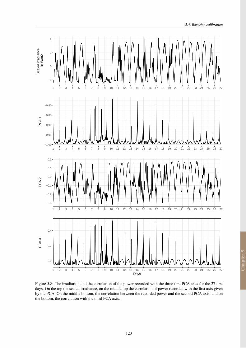
Cha

pter

5

5.4. Bayesian calibration

−1

0

1

2

1 2 3 4 5 6 7 8 9 10 11 12 13 14 15 16 17 18 19 20 21 22 23 24 25 26 27

Sca

led

irrad

ianc

e in

W/m

2

−1.00

−0.95

−0.90

−0.85

−0.80

1 2 3 4 5 6 7 8 9 10 11 12 13 14 15 16 17 18 19 20 21 22 23 24 25 26 27

PC

A 1

−0.3

−0.2

−0.1

0.0

0.1

0.2

1 2 3 4 5 6 7 8 9 10 11 12 13 14 15 16 17 18 19 20 21 22 23 24 25 26 27

PC

A 2

0.0

0.2

0.4

1 2 3 4 5 6 7 8 9 10 11 12 13 14 15 16 17 18 19 20 21 22 23 24 25 26 27

Days

PC

A 3

Figure 5.8: The irradiation and the correlation of the power recorded with the three first PCA axes for the 27 firstdays. On the top the scaled irradiance, on the middle top the correlation of power recorded with the first axis givenby the PCA. On the middle bottom, the correlation between the recorded power and the second PCA axis, and onthe bottom, the correlation with the third PCA axis.

123

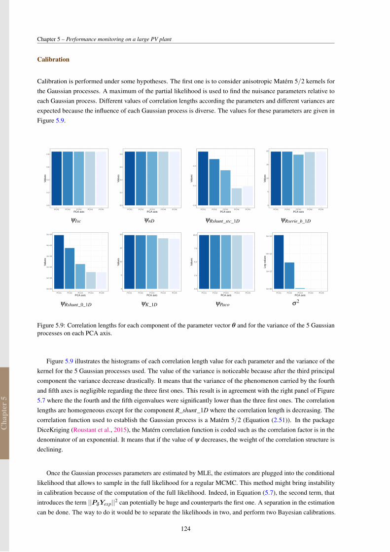
Cha

pter

5

Chapter 5 – Performance monitoring on a large PV plant

Calibration

Calibration is performed under some hypotheses. The first one is to consider anisotropic Matérn 5/2 kernels forthe Gaussian processes. A maximum of the partial likelihood is used to find the nuisance parameters relative toeach Gaussian process. Different values of correlation lengths according the parameters and different variances areexpected because the influence of each Gaussian process is diverse. The values for these parameters are given inFigure 5.9.

0.0

0.2

0.4

0.6

0.8

PCA1 PCA2 PCA3 PCA4 PCA5PCA axis

Val

ues

0.0

0.2

0.4

0.6

0.8

PCA1 PCA2 PCA3 PCA4 PCA5PCA axis

Val

ues

0.0

0.1

0.2

PCA1 PCA2 PCA3 PCA4 PCA5PCA axis

Val

ues

0

5

10

15

20

PCA1 PCA2 PCA3 PCA4 PCA5PCA axis

Val

ues

ψIsc ψnD ψRshunt_stc_1D ψRserie_b_1D

0e+00

1e−04

2e−04

3e−04

4e−04

5e−04

PCA1 PCA2 PCA3 PCA4 PCA5PCA axis

Val

ues

0

5

10

15

20

PCA1 PCA2 PCA3 PCA4 PCA5PCA axis

Val

ues

0.0

2.5

5.0

7.5

10.0

PCA1 PCA2 PCA3 PCA4 PCA5PCA axis

Val

ues

0e+00

2e+12

4e+12

6e+12

PCA1 PCA2 PCA3 PCA4 PCA5PCA axis

Log

valu

es

ψRshunt_0_1D ψK_1D ψPaco σ2

Figure 5.9: Correlation lengths for each component of the parameter vector θ and for the variance of the 5 Gaussianprocesses on each PCA axis.

Figure 5.9 illustrates the histograms of each correlation length value for each parameter and the variance of thekernel for the 5 Gaussian processes used. The value of the variance is noticeable because after the third principalcomponent the variance decrease drastically. It means that the variance of the phenomenon carried by the fourthand fifth axes is negligible regarding the three first ones. This result is in agreement with the right panel of Figure5.7 where the the fourth and the fifth eigenvalues were significantly lower than the three first ones. The correlationlengths are homogeneous except for the component R_shunt_1D where the correlation length is decreasing. Thecorrelation function used to establish the Gaussian process is a Matérn 5/2 (Equation (2.51)). In the packageDiceKriging (Roustant et al., 2015), the Matérn correlation function is coded such as the correlation factor is in thedenominator of an exponential. It means that if the value of ψ decreases, the weight of the correlation structure isdeclining.

Once the Gaussian processes parameters are estimated by MLE, the estimators are plugged into the conditionallikelihood that allows to sample in the full likelihood for a regular MCMC. This method might bring instabilityin calibration because of the computation of the full likelihood. Indeed, in Equation (5.7), the second term, thatintroduces the term ||PδYexp||2 can potentially be huge and counterparts the first one. A separation in the estimationcan be done. The way to do it would be to separate the likelihoods in two, and perform two Bayesian calibrations.

124

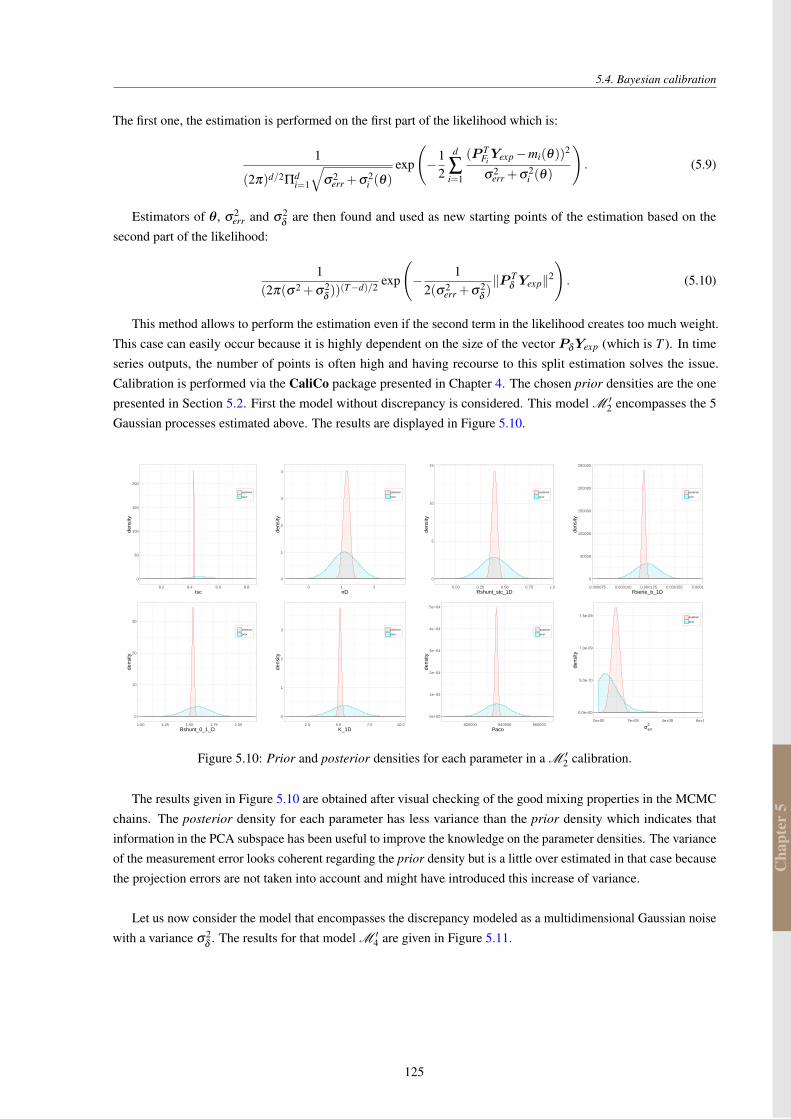
Cha

pter

5

5.4. Bayesian calibration

The first one, the estimation is performed on the first part of the likelihood which is:

1

(2π)d/2Πdi=1

√σ2

err +σ2i (θ)

exp

(−1

2

d

∑i=1

(P TFiYexp−mi(θ))

2

σ2err +σ2

i (θ)

). (5.9)

Estimators of θ, σ2err and σ2

δare then found and used as new starting points of the estimation based on the

second part of the likelihood:

1(2π(σ2 +σ2

δ))(T−d)/2 exp

(− 1

2(σ2err +σ2

δ)‖P T

δYexp‖2

). (5.10)

This method allows to perform the estimation even if the second term in the likelihood creates too much weight.This case can easily occur because it is highly dependent on the size of the vector PδYexp (which is T ). In timeseries outputs, the number of points is often high and having recourse to this split estimation solves the issue.Calibration is performed via the CaliCo package presented in Chapter 4. The chosen prior densities are the onepresented in Section 5.2. First the model without discrepancy is considered. This model M ′

2 encompasses the 5Gaussian processes estimated above. The results are displayed in Figure 5.10.

0

50

100

150

200

8.2 8.4 8.6 8.8Isc

dens

ity

posterior

prior

0

1

2

3

4

0 1 2nD

dens

ity

posterior

prior

0

5

10

15

0.00 0.25 0.50 0.75 1.00Rshunt_stc_1D

dens

ity

posterior

prior

0

50000

100000

150000

200000

250000

0.000075 0.000100 0.000125 0.000150 0.000175Rserie_b_1D

dens

ity

posterior

prior

0

10

20

30

1.00 1.25 1.50 1.75 2.00Rshunt_0_1_D

dens

ity

posterior

prior

0

1

2

3

2.5 5.0 7.5 10.0K_1D

dens

ity

posterior

prior

0e+00

1e−04

2e−04

3e−04

4e−04

5e−04

820000 840000 860000Paco

dens

ity

posterior

prior

0.0e+00

5.0e-10

1.0e-09

1.5e-09

0e+00 2e+09 4e+09 6e+09σerr

2

dens

ity

posteriorprior

Figure 5.10: Prior and posterior densities for each parameter in a M ′2 calibration.

The results given in Figure 5.10 are obtained after visual checking of the good mixing properties in the MCMCchains. The posterior density for each parameter has less variance than the prior density which indicates thatinformation in the PCA subspace has been useful to improve the knowledge on the parameter densities. The varianceof the measurement error looks coherent regarding the prior density but is a little over estimated in that case becausethe projection errors are not taken into account and might have introduced this increase of variance.

Let us now consider the model that encompasses the discrepancy modeled as a multidimensional Gaussian noisewith a variance σ2

δ. The results for that model M ′

4 are given in Figure 5.11.

125

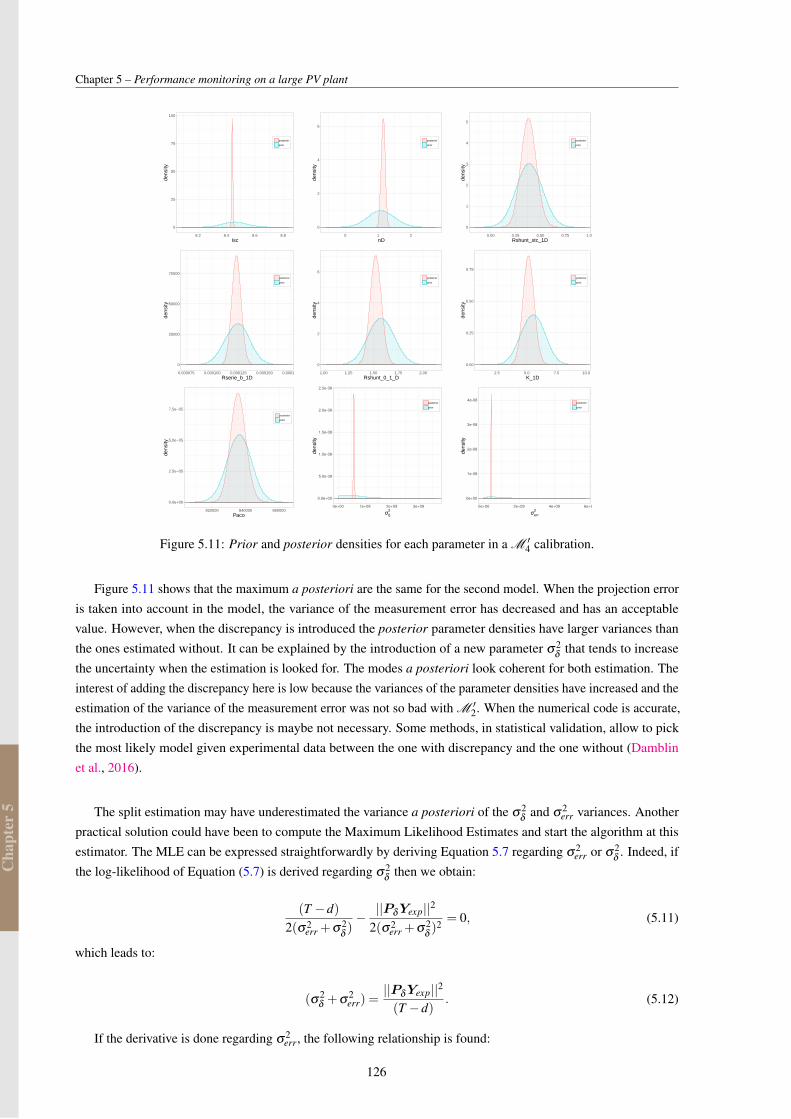
Cha

pter

5

Chapter 5 – Performance monitoring on a large PV plant

0

25

50

75

100

8.2 8.4 8.6 8.8Isc

dens

ity

posterior

prior

0

2

4

6

0 1 2nD

dens

ity

posterior

prior

0

1

2

3

4

5

0.00 0.25 0.50 0.75 1.00Rshunt_stc_1D

dens

ity

posterior

prior

0

25000

50000

75000

0.000075 0.000100 0.000125 0.000150 0.000175Rserie_b_1D

dens

ity

posterior

prior

0

2

4

6

1.00 1.25 1.50 1.75 2.00Rshunt_0_1_D

dens

ity

posterior

prior

0.00

0.25

0.50

0.75

2.5 5.0 7.5 10.0K_1D

dens

ity

posterior

prior

0.0e+00

2.5e−05

5.0e−05

7.5e−05

820000 840000 860000Paco

dens

ity

posterior

prior

0.0e+00

5.0e-09

1.0e-08

1.5e-08

2.0e-08

2.5e-08

0e+00 1e+09 2e+09 3e+09σδ

2

dens

ity

posteriorprior

0e+00

1e-08

2e-08

3e-08

4e-08

0e+00 2e+09 4e+09 6e+09σerr

2

dens

ity

posteriorprior

Figure 5.11: Prior and posterior densities for each parameter in a M ′4 calibration.

Figure 5.11 shows that the maximum a posteriori are the same for the second model. When the projection erroris taken into account in the model, the variance of the measurement error has decreased and has an acceptablevalue. However, when the discrepancy is introduced the posterior parameter densities have larger variances thanthe ones estimated without. It can be explained by the introduction of a new parameter σ2

δthat tends to increase

the uncertainty when the estimation is looked for. The modes a posteriori look coherent for both estimation. Theinterest of adding the discrepancy here is low because the variances of the parameter densities have increased and theestimation of the variance of the measurement error was not so bad with M ′

2. When the numerical code is accurate,the introduction of the discrepancy is maybe not necessary. Some methods, in statistical validation, allow to pickthe most likely model given experimental data between the one with discrepancy and the one without (Damblinet al., 2016).

The split estimation may have underestimated the variance a posteriori of the σ2δ

and σ2err variances. Another

practical solution could have been to compute the Maximum Likelihood Estimates and start the algorithm at thisestimator. The MLE can be expressed straightforwardly by deriving Equation 5.7 regarding σ2

err or σ2δ

. Indeed, ifthe log-likelihood of Equation (5.7) is derived regarding σ2

δthen we obtain:

(T −d)2(σ2

err +σ2δ)−||PδYexp||2

2(σ2err +σ2

δ)2 = 0, (5.11)

which leads to:

(σ2δ+σ

2err) =

||PδYexp||2

(T −d). (5.12)

If the derivative is done regarding σ2err, the following relationship is found:

126

Cha

pter

5

5.4. Bayesian calibration

− d2σ2

err+||PFF −PFYexp||2

2σ4err

=(T −d)

2(σ2err +σ2

δ)−||PδYexp||2

2(σ2err +σ2

δ)2 .

Thanks to Equation (5.11) the right term is equal to 0 and:

σ2err =

||PFF −PFYexp||2

d, (5.13)

σ2δ=||PδYexp||2

(T −d)−||PFF −PFYexp||2

d. (5.14)

The use of the PCA had allowed us to summarize the information contained in the time series output of the code,and to emulate the projections in a restricted space. The hypotheses made on the discrepancy can be discussed.Indeed, representing the discrepancy as the projection on the orthogonal space might be a too subtle representation.One could have think of a representation of the discrepancy as an error term on several axis and not on all theorthogonal space. The results obtained after calibration state that a numerical code which reproduces well enoughthe physical system does not need the add of the discrepancy. Regarding the results, the discrepancy just adda parameter to estimate and increases the variance a posteriori of the parameter densities. It could have beeninteresting to apply statistical validation, with the Bayes factor for example (Damblin et al., 2016), and compare theresults with the ones obtained in Chapter 3 where the discrepancy had an positive impact. The predictive aspect canalso be developed. The cross validation has not been tested on these models but a month of data could have beentaken off, calibration performed on the remaining test data set and predictive tests on the power could have beenrun on the month that have been taken off. The characterization of the meteorological data could also have beenconsidered. To get back in the frame of the article of Higdon et al. (2008), the numerical code could have beenmodified such as aX matrix, which represents the input variables, would be introduced in the input of the code.

127

Con

clus

ion

CONCLUSION AND PERSPECTIVES

The general framework of this thesis is Bayesian calibration of numerical codes. The objective was to better assesthe credibility interval a posteriori of the quantity of interest when using an industrial code. This objective is reallyimportant for industrial companies such as EDF because numerical codes are used in prediction in many contextsand these companies have difficulties to estimate the predictive error they could make. In the economical frameworkat EDF, it becomes relevant especially in the forecasting context where power plants are already built and data arealready gathered. Then, the numerical code initially used to predict the power before the construction of the plant isused again and the results are confronted with data. Calibration is then performed to better asses the knowledge ofthe input parameters of the code corresponding to the specific plant.

In this thesis, we have introduced four concepts of calibration that are using different kinds of numerical code.We reviewed the main statistical methods that are available in the literature and we have detailed the inferenceassociated with these statistical models. The purpose of the first part is to confront the models with and withoutdiscrepancy. We have noticed that, in the case of the numerical code, we used the discrepancy appears to be reallyimportant in the modeling. Indeed, the estimation of the variance of the measurement errors was not concordantwith the physical reality. Then, when the discrepancy was added, the estimation became correct which implies thatthe code was carrying an error not taken into account in the model without discrepancy. The second conclusioncomes when the initial numerical code turns out to be long to run. In this scenario case, a Gaussian process is usedto emulate the behavior of the code. In a real industrial case, numerical codes can be so expensive in time, thatwe only have recourse to a few code calls. In that case the estimations after calibration are deteriorating becausethe emulator is not precise enough. It means that the physical interpretation of the parameter density does notstand anymore and new density parameters corresponding to the, bad, emulator are found. If one is interested infinding the right parameter densities even with an emulator, it is possible to have recourse to an adaptive sequentialdesign that finds points regarding further calibration. It drastically improves the emulation quality and allows to findestimators in correspondence with a physical meaning.

Based on the models developed in the first part, I developed a package. The CaliCo package is coded inobject-oriented language that allows to manipulate easily users requests. It performs Bayesian calibration withrecourse to MCMC that are coded in C++ to improve the speed of these time consuming operations. The packageprovides flexibility on the model choice which makes it different from other packages published so far. For eachstep, visual representations are available and the user can easily take advantage of each graph. A graphical interfacehas also been developed so that EDF will be able to use the package and take advantage of the coded functions forrunning test and illustrates the improvements they could make using calibration.

The third part focuses on a real test case which brings lots of issues. Indeed, instead of having a scalar output,the code is producing time series outputs. It is a common fact for numerical codes in industries, so calibration has tobe adapted to be performed on these codes. To deal with this issue, Higdon et al. (2008) have proposed to run aPCA on a DOE that encompass the simulations of the code. The aim is to reproduce the time series output witha limited amount of Gaussian processes. Indeed the PCA allows to specify a reasonable number of axis that arecarrying a majority of the total inertia of the simulations. Then, the projected simulations on these axes are usedto estimate the parameters of the Gaussian processes (when one Gaussian process is used to emulate the behaviorof the numerical code on one axis). In this particular case we have considered the discrepancy as the projection

129

Con

clus

ion

Chapter 6 – Conclusion and perspectives

on the orthogonal subspace. We have detailed the inference associated with these statistical models and proposedand applied them on a numerical code that predicts the power of a large PV power plant. The result show that theestimation of the parameters of the code are coherent in both cases. The variance a posteriori of the parameterdensities is higher when the estimation is performed with the model with discrepancy than with the model without.However, the variance of the measurement errors is a little higher when it is estimated with the model without dis-crepancy but when the discrepancy is introduced, the value stands to decrease to have more reasonable physical sense.

The predictive aspect of the models that encompasses the PCA has to be completed. It could be interesting tovisualize how the models works in prediction. Data already gathered on the field could also be split by keeping amonth of data as a validation data set. However, with such a complex model and code, for each test set, the DOEhas to be computed again and the PCA performed at each time. Such an operation could turn out to be intractablefor desktop computers. The impact of the discrepancy is also the subject of statistical validation. Some studieshighlight the fact that data gathered on the field also allow to elect the right model. Bayes factor (Damblin, 2015) ormixture models (Kamary, 2016) have been developed and it could be interesting to try out these methods on theapplication cases provided in this thesis. Working with a time consuming code also turned out to be difficult todeal with. To run proper calibration on a function that emulates the code, this function has to be close to the initialnumerical code, otherwise the prediction of the parameter could loose their physical sense. It could be interesting tostudy deeper the way to find adapted designs for calibration or other kind of emulators. Also calibration on nestednumerical codes could be a real challenge. Indeed, emulating a nested code properly with a Gaussian process mightbe a difficult task and integrating it in a Bayesian calibration framework would be interesting for companies that areusing this kind of codes.

130

BIBLIOGRAPHY

Albert, I., Donnet, S., Guihenneuc-Jouyaux, C., Low-Choy, S., Mengersen, K., Rousseau, J., et al. (2012). Combiningexpert opinions in prior elicitation. Bayesian Analysis, 7(3):503–532.

Andrieu, C., De Freitas, N., Doucet, A., and Jordan, M. I. (2003). An introduction to mcmc for machine learning.Machine learning, 50(1-2):5–43.

Auffray, Y., Barbillon, P., and Marin, J.-M. (2010). Maximin design on non hypercube domain and kernelinterpolation. arXiv preprint arXiv:1004.0784.

Bachoc, F., Bois, G., Garnier, J., and Martinez, J.-M. (2014). Calibration and improved prediction of computermodels by universal kriging. Nuclear Science and Engineering, 176(1):81–97.

Bayarri, M. J., Berger, J. O., Paulo, R., Sacks, J., Cafeo, J. A., Cavendish, J., Lin, C.-H., and Tu, J. (2007). Aframework for validation of computer models. Technometrics, 49(2):138–154.

Bull, A. D. (2011). Convergence rates of efficient global optimization algorithms. Journal of Machine Learning

Research, 12(Oct):2879–2904.

Carmassi, M. (2018). CaliCo: Code Calibration in a Bayesian Framework. R package version 0.1.0.

Casella, G. and George, E. I. (1992). Explaining the gibbs sampler. The American Statistician, 46(3):167–174.

Chang, W. (2017). R6: Classes with Reference Semantics. R package version 2.2.2.

Cox, D. D., Park, J.-S., and Singer, C. E. (2001). A statistical method for tuning a computer code to a data base.Computational statistics & data analysis, 37(1):77–92.

Craig, P. S., Goldstein, M., Rougier, J. C., and Seheult, A. H. (2001). Bayesian forecasting for complex systemsusing computer simulators. Journal of the American Statistical Association, 96(454):717–729.

Cressie, N. A. and Noel, A. (1993). Cassie (1993). statistics for spatial data. vol. 900.

Currin, C., Mitchell, T., Morris, M., and Ylvisaker, D. (1991). Bayesian prediction of deterministic functions, withapplications to the design and analysis of computer experiments. Journal of the American Statistical Association,86(416):953–963.

Da Veiga, S. (2015). Global sensitivity analysis with dependence measures. Journal of Statistical Computation and

Simulation, 85(7):1283–1305.

Damblin, G. (2015). Contributions statistiques au calage et à la validation des codes de calcul. PhD thesis, PhDthesis, Université Paris Saclay.

Damblin, G., Barbillon, P., Keller, M., Pasanisi, A., and Parent, É. (2018). Adaptive numerical designs for thecalibration of computer codes. SIAM/ASA Journal on Uncertainty Quantification, 6(1):151–179.

Damblin, G., Couplet, M., and Iooss, B. (2013). Numerical studies of space-filling designs: optimization of latinhypercube samples and subprojection properties. Journal of Simulation, 7(4):276–289.

131

Damblin, G., Keller, M., Barbillon, P., Pasanisi, A., and Parent, É. (2016). Bayesian model selection for thevalidation of computer codes. Quality and Reliability Engineering International, 32(6):2043–2054.

De Lozzo, M. and Marrel, A. (2016). New improvements in the use of dependence measures for sensitivity analysisand screening. Journal of Statistical Computation and Simulation, 86(15):3038–3058.

Ding, J. and Radhakrishnan, R. (2008). A new method to determine the optimum load of a real solar cell using thelambert w-function. Solar Energy Materials and Solar Cells, 92(12):1566–1569.

Duffie, J. A. and Beckman, W. A. (2013). Solar engineering of thermal processes. John Wiley & Sons.

Dussert, C., Rasigni, G., Rasigni, M., Palmari, J., and Llebaria, A. (1986). Minimal spanning tree: A new approachfor studying order and disorder. Physical Review B, 34(5):3528.

Eddelbuettel, D., Francois, R., Allaire, J., Ushey, K., Kou, Q., Russell, N., Bates, D., and Chambers, J. (2018).Rcpp: Seamless R and C++ Integration. R package version 0.12.16.

Faivre, R., Iooss, B., Mahévas, S., Makowski, D., and Monod, H. (2013). Analyse de sensibilité et exploration de

modèles: application aux sciences de la nature et de l’environnement. Editions Quae.

Fang, K.-T., Li, R., and Sudjianto, A. (2005). Design and modeling for computer experiments. CRC Press.

Franco, J., Dupuy, D., Roustant, O., Damblin, G., and Iooss, B. (2015). DiceDesign: Designs of Computer

Experiments. R package version 1.7.

Franco, J., Vasseur, O., Corre, B., and Sergent, M. (2009). Minimum spanning tree: A new approach to assess thequality of the design of computer experiments. Chemometrics and intelligent laboratory systems, 97(2):164–169.

Gelman, A., Carlin, J. B., Stern, H. S., and Rubin, D. B. (1995). Bayesian data analysis. Chapman and Hall/CRC.

Gelman, A. and Rubin, D. B. (1992). Inference from iterative simulation using multiple sequences. Statistical

science, pages 457–472.

Genz, A., Bretz, F., Miwa, T., Mi, X., Leisch, F., Scheipl, F., Bornkamp, B., Maechler, M., and Hothorn, T. (2018).mvtnorm: Multivariate Normal and t Distributions. R package version 1.0-7.

Ginsbourger, D. (2009). Multiples metamodeles pour l’approximation et l’optimisation de fonctions numeriques

multivariables. PhD thesis, Ecole Nationale Supérieure des Mines de Saint-Etienne.

Gu, M. (2018a). Jointly robust prior for gaussian stochastic process in emulation, calibration and variable selection.arXiv preprint arXiv:1804.09329.

Gu, M. (2018b). RobustCalibration: Robust Calibration of Imperfect Mathematical Models. R package version0.5.1.

Gu, M. and Wang, L. (2017). Scaled gaussian stochastic process for computer model calibration and prediction.

Haario, H., Saksman, E., Tamminen, J., et al. (2001). An adaptive metropolis algorithm. Bernoulli, 7(2):223–242.

Handcock, M. S. and Stein, M. L. (1993). A bayesian analysis of kriging. Technometrics, 35(4):403–410.

Hankin, R. K. S. (2013a). approximator: Bayesian prediction of complex computer codes. R package version 1.2-6.

Hankin, R. K. S. (2013b). BACCO: Bayesian Analysis of Computer Code Output (BACCO). R package version2.0-9.

Hankin, R. K. S. (2013c). calibrator: Bayesian calibration of complex computer codes. R package version 1.2-6.

132

Hankin, R. K. S. (2014). emulator: Bayesian emulation of computer programs. R package version 1.2-15.

Hastings, W. K. (1970). Monte carlo sampling methods using markov chains and their applications. Biometrika,57(1):97–109.

Helbert, C., Dupuy, D., and Carraro, L. (2009). Assessment of uncertainty in computer experiments from universalto bayesian kriging. Applied Stochastic Models in Business and Industry, 25(2):99–113.

Higdon, D., Gattiker, J., Williams, B., and Rightley, M. (2008). Computer model calibration using high-dimensionaloutput. Journal of the American Statistical Association, 103(482):570–583.

Higdon, D., Kennedy, M., Cavendish, J. C., Cafeo, J. A., and Ryne, R. D. (2004). Combining field data andcomputer simulations for calibration and prediction. SIAM Journal on Scientific Computing, 26(2):448–466.

Hoff, P. D. (2009). A first course in Bayesian statistical methods. Springer Science & Business Media.

Husson, F., Josse, J., Le, S., and Mazet, J. (2018). FactoMineR: Multivariate Exploratory Data Analysis and Data

Mining. R package version 1.41.

Husson, F., Lê, S., and Pagès, J. (2017). Exploratory multivariate analysis by example using R. Chapman andHall/CRC.

Ishaque, K., Salam, Z., Taheri, H., et al. (2011). Modeling and simulation of photovoltaic (pv) system during partialshading based on a two-diode model. Simulation Modelling Practice and Theory, 19(7):1613–1626.

Jin, R., Chen, W., and Sudjianto, A. (2003). An efficient algorithm for constructing optimal design of computerexperiments. In ASME 2003 International Design Engineering Technical Conferences and Computers and

Information in Engineering Conference, pages 545–554. American Society of Mechanical Engineers.

Johnson, M. E., Moore, L. M., and Ylvisaker, D. (1990). Minimax and maximin distance designs. Journal of

statistical planning and inference, 26(2):131–148.

Jones, D. R., Schonlau, M., and Welch, W. J. (1998). Efficient global optimization of expensive black-box functions.Journal of Global optimization, 13(4):455–492.

Kamary, K. (2016). Non-informative priors and modelization by mixtures. PhD thesis, PhD thesis, Université ParisDauphine.

Kansa, E. (1985). Application of hardy’s multiquadric interpolation to hydrodynamics. Technical report, LawrenceLivermore National Lab.

Kennedy, M. and O’Hagan, A. (2001). Supplementary details on bayesian calibration of computer. rap. tech.,university of nottingham. Statistics Section.

Kennedy, M. C. and O’Hagan, A. (2001). Bayesian calibration of computer models. Journal of the Royal Statistical

Society: Series B (Statistical Methodology), 63(3):425–464.

Konomi, B. A., Karagiannis, G., Lai, K., and Lin, G. (2017). Bayesian treed calibration: an application to carboncapture with ax sorbent. Journal of the American Statistical Association, 112(517):37–53.

Krige, D. G. (1951). A statistical approach to some basic mine valuation problems on the witwatersrand. Journal of

the Southern African Institute of Mining and Metallurgy, 52(6):119–139.

Le Gratiet, L. (2013). Multi-fidelity Gaussian process regression for computer experiments. PhD thesis, UniversitéParis-Diderot-Paris VII.

133

Liu, F., Bayarri, M., Berger, J., et al. (2009). Modularization in bayesian analysis, with emphasis on analysis ofcomputer models. Bayesian Analysis, 4(1):119–150.

MacDoanld, B., Chipman, H., and Ranjan, P. (2015). GPfit: Gaussian Processes Modeling. R package version1.0-0.

Marrel, A. (2008). Mise en oeuvre et exploitation du métamodèle processus gaussien pour l’analyse de modèlesnumériques-application à un code de transport hydrogéologique. These de l’INSA Toulouse.

Marrel, A., Iooss, B., Laurent, B., and Roustant, O. (2009). Calculations of sobol indices for the gaussian processmetamodel. Reliability Engineering & System Safety, 94(3):742–751.

Matérn, B. (1960). Spatial variation: Meddelanden fran statens skogsforskningsinstitut. Lecture Notes in Statistics,36:21.

Matheron, G. (1963). Principles of geostatistics. Economic geology, 58(8):1246–1266.

McKay, M. D., Beckman, R. J., and Conover, W. J. (1979). Comparison of three methods for selecting values ofinput variables in the analysis of output from a computer code. Technometrics, 21(2):239–245.

Mengyang Gu, J. P. and Berger, J. (2018). RobustGaSP: Robust Gaussian Stochastic Process Emulation. R packageversion 0.5.5.

Metropolis, N., Rosenbluth, A. W., Rosenbluth, M. N., Teller, A. H., and Teller, E. (1953). Equation of statecalculations by fast computing machines. The journal of chemical physics, 21(6):1087–1092.

Mira, A. et al. (2001). On metropolis-hastings algorithms with delayed rejection. Metron, 59(3-4):231–241.

Morris, M. D. (1991). Factorial sampling plans for preliminary computational experiments. Technometrics,33(2):161–174.

Morris, M. D. and Mitchell, T. J. (1995). Exploratory designs for computational experiments. Journal of statistical

planning and inference, 43(3):381–402.

Oakley, J. E. and O’Hagan, A. (2004). Probabilistic sensitivity analysis of complex models: a bayesian approach.Journal of the Royal Statistical Society: Series B (Statistical Methodology), 66(3):751–769.

Owen, A. B. (1992). Orthogonal arrays for computer experiments, integration and visualization. Statistica Sinica,pages 439–452.

Palomo, J., Garcia-Donato, G., Paulo, R., Berger, J., Bayarri, M. J., and Sacks, J. (2017). SAVE: Bayesian Emulation,

Calibration and Validation of Computer Models. R package version 1.0.

Pearson, K. (1901). Liii. on lines and planes of closest fit to systems of points in space. The London, Edinburgh,

and Dublin Philosophical Magazine and Journal of Science, 2(11):559–572.

Petrone, G., Spagnuolo, G., and Vitelli, M. (2007). Analytical model of mismatched photovoltaic fields by means oflambert w-function. Solar energy materials and solar cells, 91(18):1652–1657.

Picault, D., Raison, B., Bacha, S., De La Casa, J., and Aguilera, J. (2010). Forecasting photovoltaic array powerproduction subject to mismatch losses. Solar Energy, 84(7):1301–1309.

Plumlee, M. (2017). Bayesian calibration of inexact computer models. Journal of the American Statistical

Association, 112(519):1274–1285.

134

Plummer, M., Best, N., Cowles, K., Vines, K., Sarkar, D., Bates, D., Almond, R., and Magnusson, A. (2016). coda:

Output Analysis and Diagnostics for MCMC. R package version 0.19-1.

Pronzato, L. and Müller, W. G. (2012). Design of computer experiments: space filling and beyond. Statistics and

Computing, 22(3):681–701.

Rasmussen, C. E. (2004). Gaussian processes in machine learning. In Advanced lectures on machine learning,pages 63–71. Springer.

Robert, C. (1996). Méthodes de Monte Carlo par chaînes de Markov. Economica.

Robert, C. (2007). The Bayesian choice: from decision-theoretic foundations to computational implementation.Springer Science & Business Media.

Robert, C. and Casella, G. (2013). Monte Carlo statistical methods. Springer Science & Business Media.

Roberts, G. O., Gelman, A., Gilks, W. R., et al. (1997). Weak convergence and optimal scaling of random walkmetropolis algorithms. The annals of applied probability, 7(1):110–120.

Rocquigny, E. d. (2009). Quantifying uncertainty in an industrial approach: an emerging consensus in an oldepistemological debate. SAPI EN. S. Surveys and Perspectives Integrating Environment and Society, (2.1).

Roustant, O., Gainsbourger, D., and Deville, Y. (2015). DiceKriging: Kriging Methods for Computer Experiments.R package version 1.5.5.

Roustant, O., Ginsbourger, D., and Deville, Y. (2012). Dicekriging, diceoptim: Two r packages for the analysisof computer experiments by kriging-based metamodelling and optimization. Journal of Statistical Software,51(1):54p.

Sacks, J., Welch, W. J., Mitchell, T. J., and Wynn, H. P. (1989). Design and analysis of computer experiments.Statistical science, pages 409–423.

Saltelli, A. (2002). Making best use of model evaluations to compute sensitivity indices. Computer physics

communications, 145(2):280–297.

Saltelli, A., Chan, K., Scott, E. M., et al. (2000). Sensitivity analysis, volume 1. Wiley New York.

Saltelli, A., Tarantola, S., Campolongo, F., and Ratto, M. (2004). Sensitivity analysis in practice: a guide to

assessing scientific models. John Wiley & Sons.

Santner, T. J., Williams, B. J., and Notz, W. I. (2013). The design and analysis of computer experiments. SpringerScience & Business Media.

Schaback, R. (2007). Convergence of unsymmetric kernel-based meshless collocation methods. SIAM Journal on

Numerical Analysis, 45(1):333–351.

Sobol’, I. M. (1990). On sensitivity estimation for nonlinear mathematical models. Matematicheskoe modelirovanie,2(1):112–118.

Sobol, I. M. (1993). Sensitivity estimates for nonlinear mathematical models. Mathematical modelling and

computational experiments, 1(4):407–414.

Stein, M. (1987). Large sample properties of simulations using latin hypercube sampling. Technometrics, 29(2):143–151.

Stein, M. L. (2012). Interpolation of spatial data: some theory for kriging. Springer Science & Business Media.

135

Sudret, B. (2008). Global sensitivity analysis using polynomial chaos expansions. Reliability Engineering & System

Safety, 93(7):964–979.

Tang, B. (1993). Orthogonal array-based latin hypercubes. Journal of the American statistical association,88(424):1392–1397.

Tian, H., Mancilla-David, F., Ellis, K., Muljadi, E., and Jenkins, P. (2012). A cell-to-module-to-array detailed modelfor photovoltaic panels. Solar energy, 86(9):2695–2706.

Tuo, R., Wu, C. J., et al. (2015). Efficient calibration for imperfect computer models. The Annals of Statistics,43(6):2331–2352.

Tuo, R. and Wu, J. (2016). A theoretical framework for calibration in computer models: parametrization, estimationand convergence properties. SIAM/ASA Journal on Uncertainty Quantification, 4(1):767–795.

Vazquez, E. and Bect, J. (2010). Convergence properties of the expected improvement algorithm with fixed meanand covariance functions. Journal of Statistical Planning and inference, 140(11):3088–3095.

Viana, F. A., Venter, G., and Balabanov, V. (2010). An algorithm for fast optimal latin hypercube design ofexperiments. International journal for numerical methods in engineering, 82(2):135–156.

Wickham, H. and Chang, W. (2016). ggplot2: Create Elegant Data Visualisations Using the Grammar of Graphics.R package version 2.2.1.

Wong, R. K., Storlie, C. B., and Lee, T. (2017). A frequentist approach to computer model calibration. Journal of

the Royal Statistical Society: Series B (Statistical Methodology), 79(2):635–648.

136

Titre : Quantification des incertitudes et calage d’un modele de centrale photovoltaıque : garantie de perfor-mance et estimation robuste de la production long-terme.

Mots cles : Centrale photovoltaıque / Calage bayesien / Quantification d’incertitudes / Code numerique

Resume : Les difficultes de mise en œuvred’experiences de terrain ou de laboratoire, ainsi queles couts associes, conduisent les societes indus-trielles a se tourner vers des codes numeriques decalcul. Ces codes, censes etre representatifs desphenomenes physiques en jeu, entraınent neanmoinstout un cortege de problemes. Le premier de cesproblemes provient de la volonte de predire larealite a partir d’un modele informatique. En ef-fet, le code doit etre representatif du phenomeneet, par consequent, etre capable de simuler desdonnees proches de la realite. Or, malgre le constantdeveloppement du realisme de ces codes, des er-reurs de prediction subsistent. Elles sont de deux na-tures differentes. La premiere provient de la differenceentre le phenomene physique et les valeurs releveesexperimentalement. La deuxieme concerne l’ecartentre le code developpe et le phenomene physique.Pour diminuer cet ecart, souvent qualifie de biais oud’erreur de modele, les developpeurs complexifienten general les codes, les rendant tres chronophages

dans certains cas. De plus, le code depend de pa-rametres a fixer par l’utilisateur qui doivent etre choi-sis pour correspondre au mieux aux donnees de ter-rain. L’estimation de ces parametres propres au codes’appelle le calage. Cette these propose dans unpremier temps une revue des methodes statistiquesnecessaires a la comprehension du calage Bayesien.Ensuite, une revue des principales methodes de ca-lage est presentee accompagnee d’un exemple com-paratif base sur un un code de calcul servant a predirela puissance d’une centrale photovoltaıque. Le pa-ckage appele CaliCo qui permet de realiser un calagerapide de beaucoup de codes numeriques est alorspresente. Enfin, un cas d’etude reel d’une grandecentrale photovoltaıque sera introduit et le calagerealise pour effectuer un suivi de performance de lacentrale. Ce cas de code industriel particulier intro-duit des specificites de calage numeriques qui serontabordees et deux modeles statistiques y seront ex-poses.

Title : Uncertainty quantification and calibration of a photovoltaic plant model: warranty of performance androbust estimation of the long-term production.

Keywords : Photovoltaic power plant / Bayesian calibration / Uncertainty quantification / Numerical code

Abstract : Field experiments are often difficult andexpensive to make. To bypass these issues, indus-trial companies have developed computational codes.These codes intend to be representative of the phy-sical system, but come with a certain amount of pro-blems. The code intends to be as close as possibleto the physical system. It turns out that, despite conti-nuous code development, the difference between thecode outputs and experiments can remain significant.Two kinds of uncertainties are observed. The firstone comes from the difference between the physi-cal phenomenon and the values recorded experimen-tally. The second concerns the gap between the codeand the physical system. To reduce this difference, of-ten named model bias, discrepancy, or model error,computer codes are generally complexified in order tomake them more realistic. These improvements lead

to time consuming codes. Moreover, a code often de-pends on parameters to be set by the user to make thecode as close as possible to field data. This estimationtask is called calibration. This thesis first proposes areview of the statistical methods necessary to unders-tand Bayesian calibration. Then, a review of the maincalibration methods is presented with a comparativeexample based on a numerical code used to predictthe power of a photovoltaic plant. The package calledCaliCo which allows to quickly perform a Bayesian ca-libration on a lot of numerical codes is then presented.Finally, a real case study of a large photovoltaic powerplant will be introduced and the calibration carried outas part of a performance monitoring framework. Thisparticular case of industrial code introduces numeri-cal calibration specificities that will be discussed withtwo statistical models.

Universite Paris-SaclayEspace Technologique / Immeuble DiscoveryRoute de l’Orme aux Merisiers RD 128 / 91190 Saint-Aubin, France