Wake and wave resistance on viscous thin films

Rene Ledesma-Alonso1,2, Michael Benzaquen1, Thomas Salez1, and Elie Raphael1

1Laboratoire de Physico-Chimie Theorique, UMR CNRS/ESPCI Gulliver 7083, 10 Rue Vauquelin,75005 Paris, France

2rene.ledesma-alonso@espci.fr

July 30, 2015

Abstract

The effect of an external pressure disturbance, being displaced with a constant speed along the free surface of aviscous thin film, is studied theoretically in the lubrication approximation in one- and two-dimensional geometries.In the comoving frame, the imposed pressure field creates a stationary deformation of the interface - a wake - thatspatially vanishes in the far region. The shape of the wake and the way it vanishes depend on both the speedand size of the external source and the properties of the film. The wave resistance, namely the force that has tobe externally furnished in order to maintain the wake, is analysed in details. For finite-size pressure disturbances,it increases with the speed, up to a certain transition value above which a monotonic decrease occurs. The roleof the horizontal extent of the pressure field is studied as well, revealing that for a smaller disturbance the lattertransition occurs at higher speed. Eventually, for a Dirac pressure source, the wave resistance either saturates in a1D geometry, or diverges in a 2D geometry.

1 Introduction

A disturbance moving along a fluid or a soft medium deforms the shape of its interface, thereby producing a wake.This is a common phenomenon, which takes place in various natural and scientific settings [8] across several ordersof magnitude, ranging from wakes generated at the surface of water [17], to perturbations in atomic Bose-Einsteincondensates [12], polariton condensates [20], and graphene plasmons [30].

The wake angle and the wave pattern generated behind a disturbance sailing at the surface of an inviscid liquidremain a topic of fundamental interest [26, 10, 4] that is also crucial for naval industry. In fact, to be maintained,the wake continually consumes energy, the latter being radiated away from the disturbance. This loss can be formu-lated into a force, called the wave resistance [14], which needs to be furnished by the controller in order to ensureconstant speed. The wave resistance associated to the capillary-gravity wake has thus been fully characterized for anincompressible inviscid flow [27, 6, 3], including the cases of Dirac [27] and finite-size [3] pressure distributions. Theperturbative role of viscosity on the inertial wave resistance has also been considered [29].

The case of highly viscous liquids is interesting as well. For instance, at the geophysical scale, the role of human-made obstacles and landscape singularities may help to understand and minimize the damages caused by naturaldisasters, such as snow avalanches [13], landslides [7], and lava or mud flows [16, 15, 19]. Similarly, gaining insight onthe effect of steady disturbances occurring during coating procedures [18] is fundamental to the industrial control ofsurface patterns. Moreover, in nanophysics, the understanding of the intrusive effect of local material probes, suchas atomic force microscopy [21, 22, 32], is crucial in order to improve further the measurement accuracy. Stateddifferently, in the context of viscous thin films [24, 31, 25, 9, 5] and in addition to the dewetting [28] and levelling [23]approaches, a moving external disturbance and the associated wake at the free surface of the film may directly be usedas a new kind of fine rheological probe [11, 1]. This idea was even proposed as a possible method to measure slip atthe solid-liquid boundary [2]. Interestingly, despite the broad applicability of the lubrication theory that describes allthe examples of this paragraph, the study of the wave resistance in such a context remains an open question.

In the present study, the surface pattern generated by a moving external pressure disturbance along a viscous thinfilm is described theoretically, within the lubrication approximation, for one- and two-dimensional systems. The waveresistance is analyzed in both cases, leading to analytical expressions of this force in terms of the disturbance speedand size, and the physical properties of the liquid film. Low- and high-speed regimes are described through asymptoticexpressions, which unveil the nature of the wave resistance in the lubrication context.

1

arX

iv:1

507.

0742

5v1

[ph

ysic

s.fl

u-dy

n] 2

7 Ju

l 201

5

2 GENERAL CASE

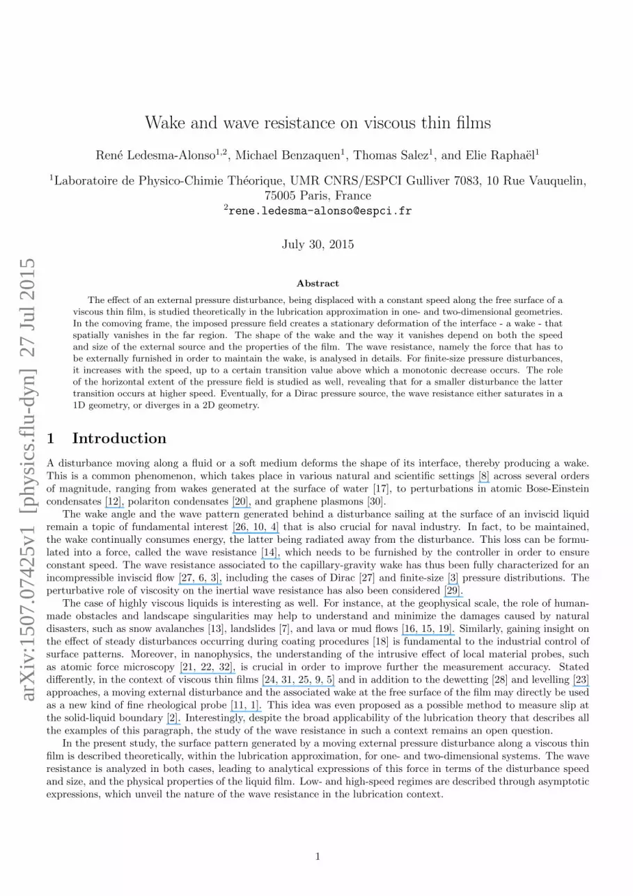
Figure 1 Schematic diagram of the surface profile h of a viscous thin film reacting to an external pressure disturbance ψmoving along time t at constant speed v. (a) 1D and (b) 2D geometries.

2 General case

2.1 Thin-film equation for a moving pressure disturbance

We consider a viscous liquid film of thickness h0 deposited over a flat horizontal substrate. The equilibrium free surfaceof the film is flat as well, and perpendicular to the vertical direction z. An external pressure field ψ, moving alongthe horizontal direction x with constant speed v ≥ 0, is applied over the liquid film. As a result, a stationary surfacepattern h is observed (see Fig. 1) in the frame of reference of the moving disturbance.

The pressure jump plg at the liquid-gas interface, with respect to the atmospheric pressure, is given by the Young-Laplace equation which reads for small slopes:

plg = −γ∆h+ ρgh+ ψ , (1)

where ∆ denotes the Laplacian operator in cartesian coordinates, g is the acceleration of gravity, and γ and ρ are theliquid-gas surface tension and density difference, respectively. In the lubrication theory, conservation of volume yieldsthe following Reynolds equation[25]:

∂h

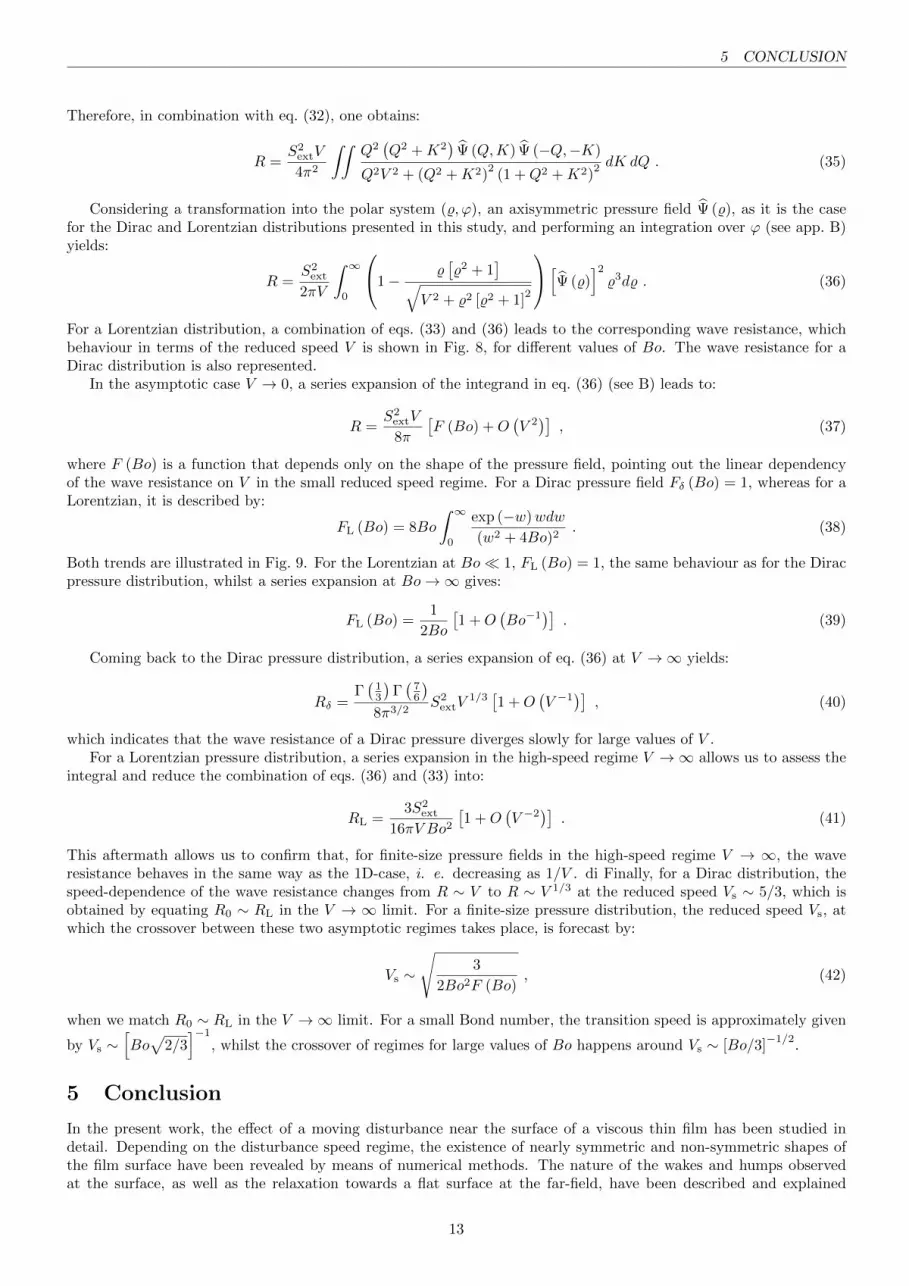
∂t= ∇ ·

[(h0 + h)

3

3µ∇plg

], (2)

where µ is the dynamic shear viscosity of the liquid. Equations (1) and (2) are coupled, and should be solved togetherin order to describe the dynamic response of the viscous thin film due to the displacement of the external pressurefield.

We introduce the dimensionless variables:

X = κx, Y = κy,

H =h

h0, T =

t

τ,

Ψ =ψ`

sextκ, Sext =

sextκ

ρgh0`, (3)

where the capillary length κ−1 =√γ/(ρg) has been chosen as the characteristic horizontal length scale, τ =

3µγ/[(ρg)2h30

]is the visco-capillary time scale, and sext =

∫ ∫dxdy ψ is the imposed load where in 1D the inte-

gral over y is restricted to a chosen horizontal extent Ly. Finally, ` is a reference length scale that depends on thedimension of the system: in 1D one sets ` = Ly, and in 2D one sets ` = κ−1. In the limit of small surface deformationsH 1, the thin-film equation (TFE), obtained from the combination of eqs. (1) and (2), is given by:

∂H

∂T= −∇ · [∇ (∆H)−∇H − Sext∇Ψ] . (4)

2

2.2 Wave resistance 3 ONE-DIMENSIONAL CASE

Let us introduce the capillary number Ca = µv/γ and the Bond number Bo = ρga2/γ, where a denotes thecharacteristic horizontal size of the external pressure field. We now place ourselves in the frame of reference of themoving disturbance, through the new variable U = X − V T , where the reduced speed V reads:

V = vτκ . (5)

By assuming stationarity of the surface profile in this comoving frame, one has H (X,Y, T ) = ζ (U, Y ) and thus eq. (4)reduces to the partial differential equation:[

∂2

∂U2+

∂2

∂Y 2

]2ζ −

[∂2

∂U2+

∂2

∂Y 2

]ζ − V ∂ζ

∂U

= Sext

[∂2

∂U2+

∂2

∂Y 2

]Ψ . (6)

In the following, we refer to eq. (6) as the 2D-TFE.Similarly, for a 1D geometry, in which the system is invariant with respect to the Y -direction, eq. (4) is reduced

to the ordinary differential equation:

d

dU

[d3ζ

dU3− dζ

dU− V ζ

]= Sext

d2Ψ

dU2. (7)

After integrating once with respect to U , and considering the boundary conditions ζ = 0, dζ/dU = 0, d3ζ/dU3 = 0,and dΨ/dU = 0 at |U | → ∞, one gets:

d3ζ

dU3− dζ

dU− V ζ = Sext

dΨ

dU. (8)

In the following, we refer to eq. (8) as the 1D-TFE.

2.2 Wave resistance

The wave resistance r is the force that has to be externally furnished by the operator – i. e. the pressure field – inorder to maintain the wake. According to Havelock’s formula [14], it reads:

r =

∫ ∫ψ (x, y)

∂h

∂xdx dy , (9)

where in the 1D case the integral over y is restricted to the chosen horizontal extent Ly. Defining the dimensionlesswave resistance R through:

R =r

ρgh20`, (10)

and recalling eq. (3), one gets in the comoving frame:

R =Sext

κ`

∫ ∫Ψ (U, Y )

∂ζ

∂UdU dY . (11)

In the next two sections, we solve the 1D-TFE and 2D-TFE using Fourier analysis, and study the shape of theirsolutions and the wave resistance for different values of the two relevant dimensionless parameters: the reduced speedV and the Bond number Bo. Note that, by linearity of the response, all the results correspond to an arbitrary thirddimensionless number Sext, the dimensionless load, as it can be absorbed in ζ. In the following, Sext is chosen to bepositive, although the physical foundations and the wave resistance are valid for any sign of Sext.

3 One-dimensional case

3.1 Surface profile

Considering the one-dimensional Fourier transforms ζ (Q) and Ψ (Q) (see app. A) of the surface profile and the pressurefield, the 1D-TFE given in eq. (8) becomes:

−(iQ3 + iQ+ V

)ζ = iQSextΨ , (12)

3

3.1 Surface profile 3 ONE-DIMENSIONAL CASE

space

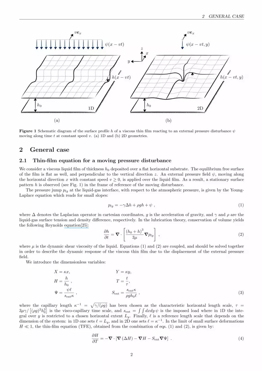
Figure 2 Normalized surface profile ζ(U), solution of eq. (8) as given by eq. (13), using Lorentzian (see eq. (14)) and Dirac(Bo→ 0) 1D pressure distributions, with dimensionless load Sext > 0, for different values of the reduced speed V and theBond number Bo, as indicated.

4

3.1 Surface profile 3 ONE-DIMENSIONAL CASE

V0.01 0.1 1 10 100 1000

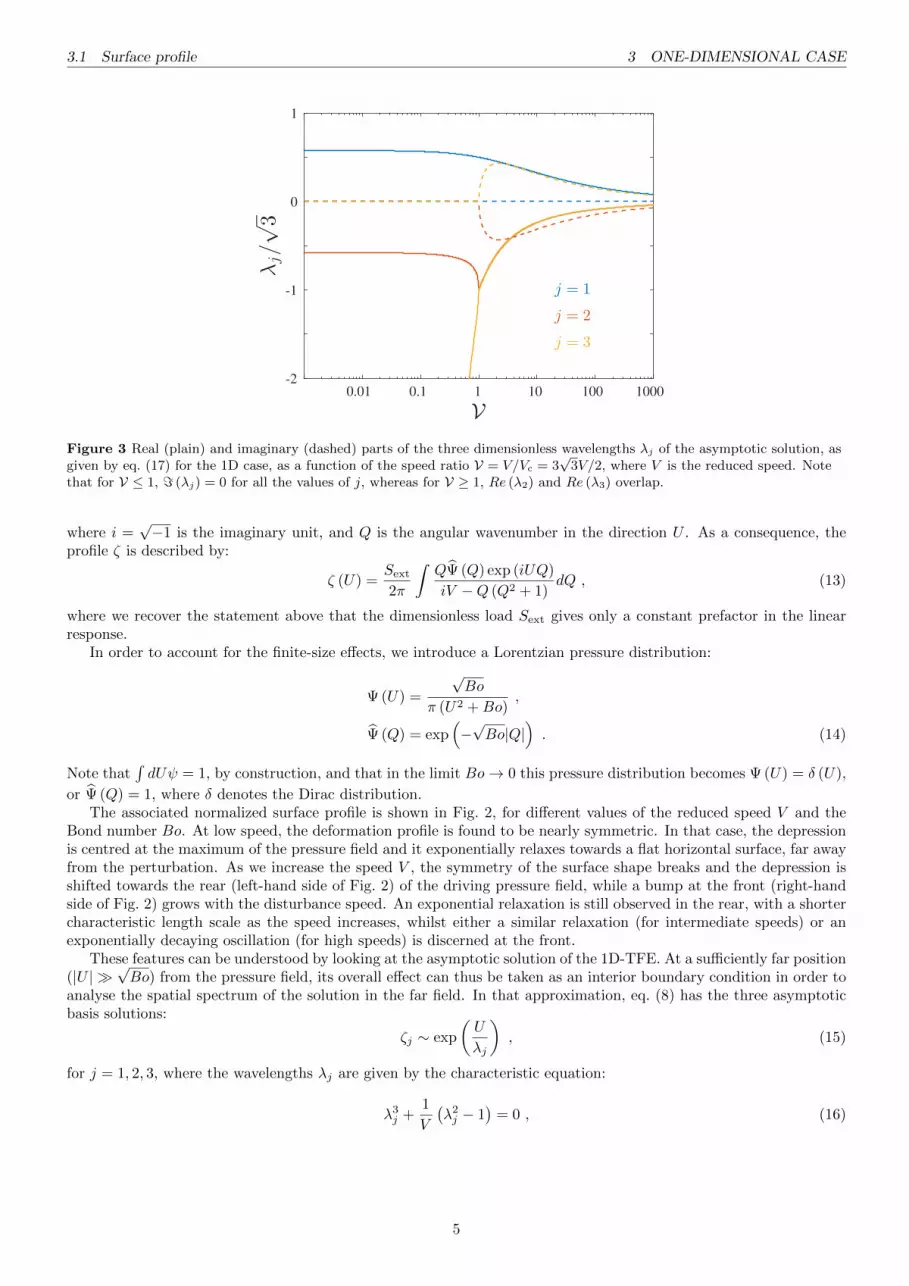
λj/√3

-2

-1

0

1

j = 1

j = 2

j = 3

Figure 3 Real (plain) and imaginary (dashed) parts of the three dimensionless wavelengths λj of the asymptotic solution, asgiven by eq. (17) for the 1D case, as a function of the speed ratio V = V/Vc = 3

√3V/2, where V is the reduced speed. Note

that for V ≤ 1, = (λj) = 0 for all the values of j, whereas for V ≥ 1, Re (λ2) and Re (λ3) overlap.

where i =√−1 is the imaginary unit, and Q is the angular wavenumber in the direction U . As a consequence, the

profile ζ is described by:

ζ (U) =Sext

2π

∫QΨ (Q) exp (iUQ)

iV −Q (Q2 + 1)dQ , (13)

where we recover the statement above that the dimensionless load Sext gives only a constant prefactor in the linearresponse.

In order to account for the finite-size effects, we introduce a Lorentzian pressure distribution:

Ψ (U) =

√Bo

π (U2 +Bo),

Ψ (Q) = exp(−√Bo|Q|

). (14)

Note that∫dUψ = 1, by construction, and that in the limit Bo→ 0 this pressure distribution becomes Ψ (U) = δ (U),

or Ψ (Q) = 1, where δ denotes the Dirac distribution.The associated normalized surface profile is shown in Fig. 2, for different values of the reduced speed V and the

Bond number Bo. At low speed, the deformation profile is found to be nearly symmetric. In that case, the depressionis centred at the maximum of the pressure field and it exponentially relaxes towards a flat horizontal surface, far awayfrom the perturbation. As we increase the speed V , the symmetry of the surface shape breaks and the depression isshifted towards the rear (left-hand side of Fig. 2) of the driving pressure field, while a bump at the front (right-handside of Fig. 2) grows with the disturbance speed. An exponential relaxation is still observed in the rear, with a shortercharacteristic length scale as the speed increases, whilst either a similar relaxation (for intermediate speeds) or anexponentially decaying oscillation (for high speeds) is discerned at the front.

These features can be understood by looking at the asymptotic solution of the 1D-TFE. At a sufficiently far position(|U |

√Bo) from the pressure field, its overall effect can thus be taken as an interior boundary condition in order to

analyse the spatial spectrum of the solution in the far field. In that approximation, eq. (8) has the three asymptoticbasis solutions:

ζj ∼ exp

(U

λj

), (15)

for j = 1, 2, 3, where the wavelengths λj are given by the characteristic equation:

λ3j +1

V

(λ2j − 1

)= 0 , (16)

5

3.2 Wave resistance 3 ONE-DIMENSIONAL CASE

and thus:

λj =√

3

(Ω

σj+σjΩ

)−1,

σj = exp

[i2π

3(j − 1)

],

Ω =3

√V +

√V2 − 1 . (17)

Here, V is the speed ratio V = V/Vc defined from the critical speed Vc = 2/(3√

3). The dependence of λj on V isdepicted in Fig. 3. Since Ω comes from an expression which may have different values (the roots of Ω6 − 2VΩ3 + 1)

we note that the correct value to be employed in eq. (17) satisfies the relation [< (Ω)]2

= 1− [= (Ω)]2

for V ≤ 1, and= (Ω) = 0 for V ≥ 1.

According to the signs of λj in Fig. 3, and in order to avoid any divergence of the profile at U = −∞, it follows

that for U < 0 and |U | √Bo the shape of the surface is necessarily given by:

ζ = N1 exp

(U

λ1

), (18)

where N1 is a real constant and λ1 takes a real value <(λ1) > 0. This indicates that the surface always presents apure exponential relaxation towards a flat horizontal profile at the rear of the perturbation, in the far field, no matterthe speed. The typical distance λ1 over which this relaxation occurs becomes shorter as V increases, as observed inFig. 2.

On the other hand, for U > 0 and |U | √Bo, the behaviour of the asymptotic solution depends strongly on V.

When V < 1, according to the signs of λj in Fig. 3, and in order to avoid any divergence of the profile at U = +∞,the surface profile is described in the far field by the superposition:

ζ = N2 exp

(U

λ2

)+N3 exp

(U

λ3

), (19)

where N2 and N3 are real constants, and λ2 and λ3 are both real and negative with |λ2| < |λ3|. As a consequence,an over-damping of the surface perturbation is observed in the far field. The V = 1 case corresponds to the criticaldamping situation for which λ2 = λ3 = −1. Finally, for V > 1, λ2 and λ3 are complex conjugates, and so are thecorresponding amplitudes N2 and N3. Thus, one can write:

ζ = N exp

[< (λ2)U

< (λ2)2

+ = (λ2)2

]cos

[= (λ2)U

< (λ2)2

+ = (λ2)2 + φ

], (20)

where N and φ are real constants. This indicates the presence of spatial oscillations at the front of the perturbation inthe far field, before the film surface attains its complete relaxation. In brief, the critical speed Vc denotes the reducedspeed V at which a transition is observed from overdamped relaxation to damped oscillations, at the front of theperturbation.

In addition to the far-field trends described above, that depend solely on the reduced speed V and the associateddimensionless characteristic lengths λj , one can discern in Fig. 2 different near-field behaviours of the surface profiles

that involve a second dimensionless length√Bo associated with the horizontal extent of the pressure field. As already

explained above, for a pressure distribution with sufficiently small size (√Bo 1), the healing length of the profile is

almost independent of Bo, and approximately given by λj that decreases as V increases. In contrast, for a large size

(√Bo 1), the lateral extent of the profile is comparable with the typical size

√Bo of the pressure disturbance, as

can be observed at low speed V in Fig. 2. In this√Bo 1 case, the healing length decreases with increasing speed

only for low velocities. Above the critical speed Vc typically, the healing length saturates, leading to surface profilesthat nearly follow the same trend, independently of V .

3.2 Wave resistance

Invoking eq. (11) and the fact that in 1D one has ` = Ly, one gets the following 1D expression of the dimensionlesswave resistance:

R = Sext

∫Ψ (U)

dζ

dUdU . (21)

For a viscous thin film, it can be shown that the power exerted by the wave resistance equals the viscous dissipatedpower in the bulk (see app. A, eq. (58)). This power balance highlights the fact that the wave resistance is the force

6

3.2 Wave resistance 3 ONE-DIMENSIONAL CASE

log(V )-6 -3 0 3 6

log(R

/S2 ext)

-12

-9

-6

-3

0

Dirac

1/6

1

1

1

1

log(B

o)

4

2

0

-2

-4

Figure 4 Dimensionless wave resistance R (see eq. (22)) normalized by the square of the dimensionless load Sext, as a functionof the reduced speed V , for a 1D Dirac pressure distribution, and for a 1D Lorentzian pressure distribution (see eq. (14)) withdifferent values of the Bond number Bo as indicated. The vertical dashed lines indicate the crossover speeds Vs, estimatedfrom eq. (30) for different Bo. The horizontal dotted line corresponds to the plateau value of 1/6 in the 1D Dirac case.

log(Bo)-6 -3 0 3 6

log(f)

-2

-1

0

2

1

π/4

Lorentz

Dirac

Figure 5 Shape function f (see eq. (23)) of the 1D pressure field in the low-speed regime, as a function of the Bond numberBo. Both the Lorentzian (plain, see eq. (24)) and the Dirac (dashed, see text) cases are represented.

7

4.1 Surface profile 4 TWO-DIMENSIONAL CASE

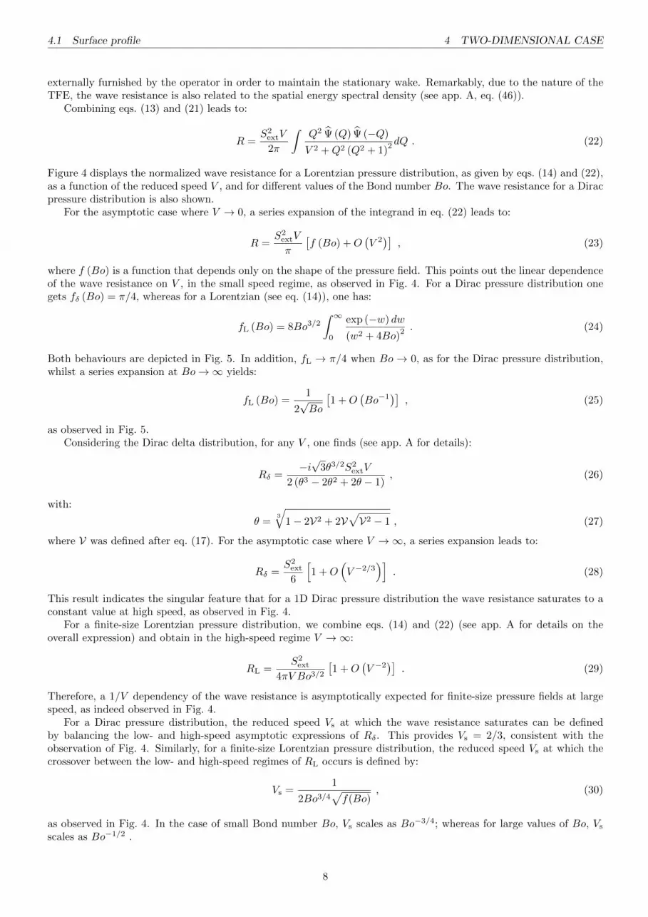
externally furnished by the operator in order to maintain the stationary wake. Remarkably, due to the nature of theTFE, the wave resistance is also related to the spatial energy spectral density (see app. A, eq. (46)).

Combining eqs. (13) and (21) leads to:

R =S2extV

2π

∫Q2 Ψ (Q) Ψ (−Q)

V 2 +Q2 (Q2 + 1)2 dQ . (22)

Figure 4 displays the normalized wave resistance for a Lorentzian pressure distribution, as given by eqs. (14) and (22),as a function of the reduced speed V , and for different values of the Bond number Bo. The wave resistance for a Diracpressure distribution is also shown.

For the asymptotic case where V → 0, a series expansion of the integrand in eq. (22) leads to:

R =S2extV

π

[f (Bo) +O

(V 2)]

, (23)

where f (Bo) is a function that depends only on the shape of the pressure field. This points out the linear dependenceof the wave resistance on V , in the small speed regime, as observed in Fig. 4. For a Dirac pressure distribution onegets fδ (Bo) = π/4, whereas for a Lorentzian (see eq. (14)), one has:

fL (Bo) = 8Bo3/2∫ ∞0

exp (−w) dw

(w2 + 4Bo)2 . (24)

Both behaviours are depicted in Fig. 5. In addition, fL → π/4 when Bo → 0, as for the Dirac pressure distribution,whilst a series expansion at Bo→∞ yields:

fL (Bo) =1

2√Bo

[1 +O

(Bo−1

)], (25)

as observed in Fig. 5.Considering the Dirac delta distribution, for any V , one finds (see app. A for details):

Rδ =−i√

3θ3/2S2extV

2 (θ3 − 2θ2 + 2θ − 1), (26)

with:

θ =3

√1− 2V2 + 2V

√V2 − 1 , (27)

where V was defined after eq. (17). For the asymptotic case where V →∞, a series expansion leads to:

Rδ =S2ext

6

[1 +O

(V −2/3

)]. (28)

This result indicates the singular feature that for a 1D Dirac pressure distribution the wave resistance saturates to aconstant value at high speed, as observed in Fig. 4.

For a finite-size Lorentzian pressure distribution, we combine eqs. (14) and (22) (see app. A for details on theoverall expression) and obtain in the high-speed regime V →∞:

RL =S2ext

4πV Bo3/2[1 +O

(V −2

)]. (29)

Therefore, a 1/V dependency of the wave resistance is asymptotically expected for finite-size pressure fields at largespeed, as indeed observed in Fig. 4.

For a Dirac pressure distribution, the reduced speed Vs at which the wave resistance saturates can be definedby balancing the low- and high-speed asymptotic expressions of Rδ. This provides Vs = 2/3, consistent with theobservation of Fig. 4. Similarly, for a finite-size Lorentzian pressure distribution, the reduced speed Vs at which thecrossover between the low- and high-speed regimes of RL occurs is defined by:

Vs =1

2Bo3/4√f(Bo)

, (30)

as observed in Fig. 4. In the case of small Bond number Bo, Vs scales as Bo−3/4; whereas for large values of Bo, Vsscales as Bo−1/2 .

8

4.1 Surface profile 4 TWO-DIMENSIONAL CASE

Figure 6 Normalized thin-film surface profile in presence of a moving Lorentzian pressure disturbance, with dimensionlessload Sext > 0, Bond number Bo = 102, and reduced speed V = 10, computed from eqs. (32) and (33). Perspective views of thefront (top) and the back (bottom), in arbitrary units and colour code.

9

4.1 Surface profile 4 TWO-DIMENSIONAL CASE

U-20 -10 0

Y

10

0

-10

U-20 -10 0

U-20 -10 0

Y

-10

0

10

Y

-10

0

10

Y

-10

0

10

Y

-10

0

10

ζ/max

(−ζ)

-1

-0.8

-0.6

-0.4

-0.2

0

0.2

log (Bo)-2 0 2

log(V

)

-2

-1

0

1

2

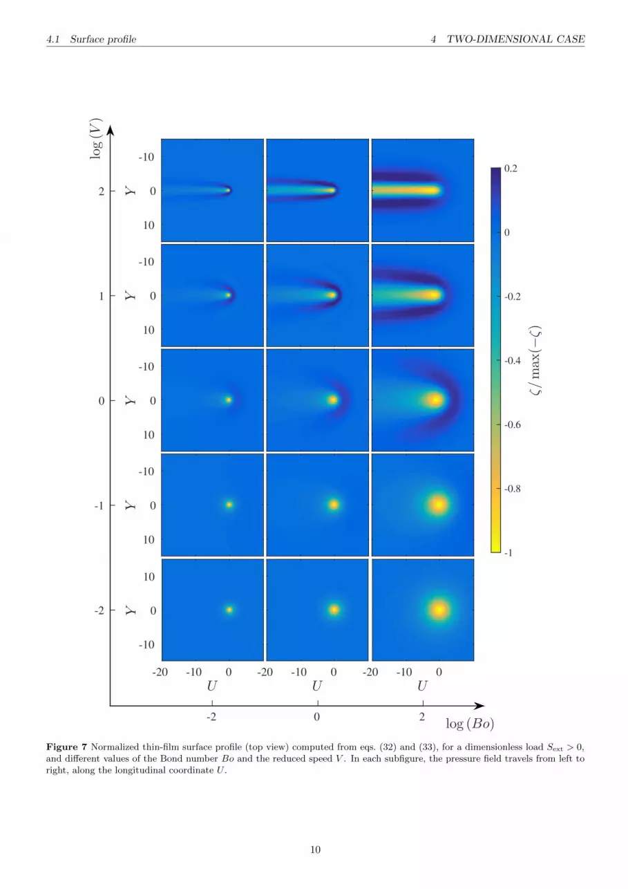
Figure 7 Normalized thin-film surface profile (top view) computed from eqs. (32) and (33), for a dimensionless load Sext > 0,and different values of the Bond number Bo and the reduced speed V . In each subfigure, the pressure field travels from left toright, along the longitudinal coordinate U .

10

4 TWO-DIMENSIONAL CASE

4 Two-dimensional case

4.1 Surface profile

Considering the two-dimensional Fourier transforms ζ (Q,K) and Ψ (Q,K) of the surface profile and the pressure field,with the definitions given in app. B, the 2D-TFE of eq. (6) becomes:[

iQV −(Q2 +K2

)2 − (Q2 +K2)]ζ = Sext

(Q2 +K2

)Ψ , (31)

where Q and K are the spatial angular frequencies in the U and Y -directions, respectively. Consequently, the surfaceζ (U, Y ) of the thin film reads:

ζ =Sext

4π2

∫∫ (Q2 +K2

)exp [i (QU +KY )] Ψ (Q,K)

iQV − (Q2 +K2) (1 +Q2 +K2)dKdQ . (32)

In analogy with the previous 1D case, we introduce the following 2D axisymmetric finite-size Lorentzian pressuredistribution:

Ψ (U, Y ) =

√Bo

2π (U2 + Y 2 +Bo)3/2

,

Ψ (Q,K) = exp[−√Bo (Q2 +K2)

]. (33)

We recall that, since a is the characteristic horizontal size of the pressure field,√Bo = aκ is the dimensionless size.

When, Bo→ 0, the Dirac pressure distribution Ψ (U, Y ) = δ(U)δ(Y ), or its equivalent Ψ (Q,K) = 1 in the frequencydomain, is recovered.

Surface patterns generated by a Lorentzian pressure disturbance, for several combinations of the parameters Boand V , are illustrated in Figs. 6 and 7. A common feature of these profiles is the depression observed. In Fig. 6, dueto the particular parameters employed (see caption) to generate the surface profile, a non-symmetric shape is shown.A rim surrounds the front of the depression and becomes a wake, behind, that follows the straight translation path ofthe pressure distribution along U .

In Fig. 7, for low speeds (V < 1), we find deformation profiles which are mostly symmetric, with a main depressionaligned with the maximum of the pressure field and followed by a monotonic relaxation towards a flat horizontalsurface. In this situation, the liquid-film surface relaxation occurs faster than the displacement of the pressure field:in real units, the displacement speed v is smaller than the characteristic speed ρgh30κ/3µ at which the film relaxes andthus propagates information at its surface. As the pressure acts on the surface by creating a moving depression, thefilm has enough time to move the dislodged liquid volume isotropically.

Like for the 1D case, an increase of the speed V induces a symmetry breaking phenomenon, which above V ' 1consists of a level rising at the front (right-hand side of the corresponding subfigures of Fig. 7) and a wake at the rear(left-hand side). In real units, the relaxation of the liquid film now occurs with a speed ρgh30κ/3µ which is smallerthan the displacement speed v of the pressure field. In other words, the liquid volume that is ejected by the appliedpressure is not distributed isotropically because the information at the film surface does not propagate fast enough.This retardation effect is similar to the Mach and Cerenkov physics [8], where the speed of the object becomes largerthan the wave-propagation speed in the considered medium.

For relatively moderate speeds, V ' 1, the protuberance at the front covers a crescent-shaped region that growswith the size of the pressure field

√Bo. The maximum surface level at the front of the pressure field is located at

Y = 0, whereas the maximum of the wake, at each position U < 0, is located at Y ∼ |U |1/2. In contrast, the localminimum of the wake is always placed at Y = 0. In addition, both the local maximum and minimum of the wakepresent a rapid spatial exponential relaxation. As the speed grows in the range V ∈

[1, 102

], the height of the frontal

rim reduces, while the extent of the wake in the rear reaches a larger distance. The local maximum at the front is stilllocated at Y = 0, while the maximum height of the wake is now placed at Y ∼ |U |α, where the exponent α evolvesfrom 1/2 at V ∼ 1 to 1/4 at V ∼ 102. Interestingly, in contrast to the inertial wake [17, 10], we note the absence of awell-defined angle in the present lubrication wake.

4.2 Wave resistance

Invoking eq. (11) and the fact that in 2D one has ` = κ−1, one gets the following 2D expression of the dimensionlesswave resistance:

R = Sext

∫∫Ψ (U, Y )

∂ζ

∂UdUdY . (34)

11

4.2 Wave resistance 4 TWO-DIMENSIONAL CASE

log(V )-6 -3 0 3 6

log(R

/S2 ext)

-12

-9

-6

-3

0

Dirac

11

1

1

3

1

log(B

o)

4

2

0

-2

-4

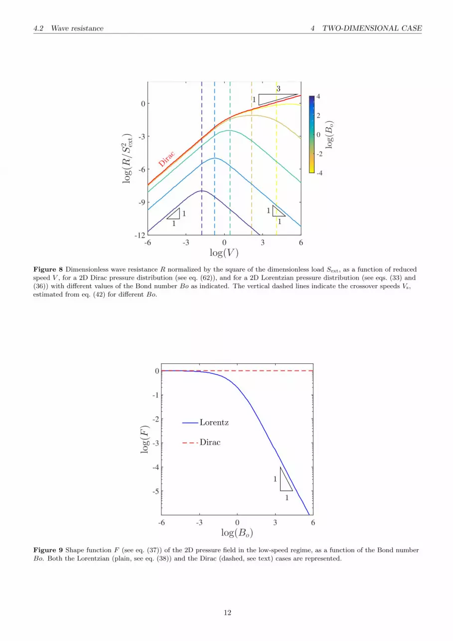
Figure 8 Dimensionless wave resistance R normalized by the square of the dimensionless load Sext, as a function of reducedspeed V , for a 2D Dirac pressure distribution (see eq. (62)), and for a 2D Lorentzian pressure distribution (see eqs. (33) and(36)) with different values of the Bond number Bo as indicated. The vertical dashed lines indicate the crossover speeds Vs,estimated from eq. (42) for different Bo.

log(Bo)-6 -3 0 3 6

log(F

)

-5

-4

-3

-2

-1

0

1

1

Lorentz

Dirac

Figure 9 Shape function F (see eq. (37)) of the 2D pressure field in the low-speed regime, as a function of the Bond numberBo. Both the Lorentzian (plain, see eq. (38)) and the Dirac (dashed, see text) cases are represented.

12

5 CONCLUSION

Therefore, in combination with eq. (32), one obtains:

R =S2extV

4π2

∫∫Q2(Q2 +K2

)Ψ (Q,K) Ψ (−Q,−K)

Q2V 2 + (Q2 +K2)2

(1 +Q2 +K2)2 dK dQ . (35)

Considering a transformation into the polar system (%, ϕ), an axisymmetric pressure field Ψ (%), as it is the casefor the Dirac and Lorentzian distributions presented in this study, and performing an integration over ϕ (see app. B)yields:

R =S2ext

2πV

∫ ∞0

1−%[%2 + 1

]√V 2 + %2 [%2 + 1]

2

[Ψ (%)]2%3d% . (36)

For a Lorentzian distribution, a combination of eqs. (33) and (36) leads to the corresponding wave resistance, whichbehaviour in terms of the reduced speed V is shown in Fig. 8, for different values of Bo. The wave resistance for aDirac distribution is also represented.

In the asymptotic case V → 0, a series expansion of the integrand in eq. (36) (see B) leads to:

R =S2extV

8π

[F (Bo) +O

(V 2)]

, (37)

where F (Bo) is a function that depends only on the shape of the pressure field, pointing out the linear dependencyof the wave resistance on V in the small reduced speed regime. For a Dirac pressure field Fδ (Bo) = 1, whereas for aLorentzian, it is described by:

FL (Bo) = 8Bo

∫ ∞0

exp (−w)wdw

(w2 + 4Bo)2. (38)

Both trends are illustrated in Fig. 9. For the Lorentzian at Bo 1, FL (Bo) = 1, the same behaviour as for the Diracpressure distribution, whilst a series expansion at Bo→∞ gives:

FL (Bo) =1

2Bo

[1 +O

(Bo−1

)]. (39)

Coming back to the Dirac pressure distribution, a series expansion of eq. (36) at V →∞ yields:

Rδ =Γ(13

)Γ(76

)8π3/2

S2extV

1/3[1 +O

(V −1

)], (40)

which indicates that the wave resistance of a Dirac pressure diverges slowly for large values of V .For a Lorentzian pressure distribution, a series expansion in the high-speed regime V →∞ allows us to assess the

integral and reduce the combination of eqs. (36) and (33) into:

RL =3S2

ext

16πV Bo2[1 +O

(V −2

)]. (41)

This aftermath allows us to confirm that, for finite-size pressure fields in the high-speed regime V → ∞, the waveresistance behaves in the same way as the 1D-case, i. e. decreasing as 1/V . di Finally, for a Dirac distribution, thespeed-dependence of the wave resistance changes from R ∼ V to R ∼ V 1/3 at the reduced speed Vs ∼ 5/3, which isobtained by equating R0 ∼ RL in the V → ∞ limit. For a finite-size pressure distribution, the reduced speed Vs, atwhich the crossover between these two asymptotic regimes takes place, is forecast by:

Vs ∼

√3

2Bo2F (Bo), (42)

when we match R0 ∼ RL in the V →∞ limit. For a small Bond number, the transition speed is approximately given

by Vs ∼[Bo√

2/3]−1

, whilst the crossover of regimes for large values of Bo happens around Vs ∼ [Bo/3]−1/2

.

5 Conclusion

In the present work, the effect of a moving disturbance near the surface of a viscous thin film has been studied indetail. Depending on the disturbance speed regime, the existence of nearly symmetric and non-symmetric shapes ofthe film surface have been revealed by means of numerical methods. The nature of the wakes and humps observedat the surface, as well as the relaxation towards a flat surface at the far-field, have been described and explained

13

REFERENCES

through asymptotic solutions, unveiling their reliance on several dimensionless parameters: Bo, Sext and V , whichare obviously related to the geometrical and physical properties of the liquid film: ρ, γ, µ, h0 and the pressuredistribution: Sext and a.

In addition, the wave resistance, which one must be overcome in order to displace the disturbance at a constantspeed, has been analysed. Even though the shape of the free surface of the thin film is only recovered numerically, thewave resistance can be accurately derived in different asymptotic speed regimes, by means of analytical expressionsfor a Dirac delta and a Lorentzian pressure distributions. An overall expression for the wave resistance in the 1D casehas been presented.

We believe that the wave resistance, which full characterization has been presented in this article, can be employedto deduce one of the physical properties of a viscous thin film, such as ρ, γ, µ or h0, when the remaining are knowna priori.

6 Acknowledgements

We thank P. Tordjeman, D. Legendre and A. Darmon for fruitful discussions.

References[1] N. Alleborn and H. Raszillier. Local perturbation of thin film flow. Arch. Appl. Mech., 73:734–751, 2004.

[2] N. Alleborn, A. Sharma, and A. Delgado. Probing of thin slipping films by persistent externql disturbances. Can. J. Chem. Eng.,85:586–597, 2007.

[3] M. Benzaquen, F. Chevy, and E. Raphael. Wave resistance for capillary gravity waves: Finite-size effects. Europhys. Lett., 96(34003):1–5, 2011.

[4] M. Benzaquen, A. Darmon, and E. Raphael. Wake pattern and wave resistance for anisotropic moving disturbances. Phys. Fluids.,26(092106):1–7, 2014.

[5] R. Blossey. Thin liquid films. Springer, 2012.

[6] T. Burghelea and V. Steinberg. Wave drag due to generation of capillari-gravity surface waves. Phys. Rev. E, 66(051204):1–13, 2002.

[7] C. S. Campbell. J. Geol., 97:653, 1989.

[8] I. Carusotto and G. Rousseaux. The cerenkov effect revisited: From swimming ducks to zero modes in gravitational analogues.Analogue Gravity Phenomenology, in Lecture Notes in Physics, 870:109–144, 2013.

[9] R. V. Craster and O. K. Matar. Dynamics and stability of thin liquid films. Rev. Mod. Phys., 81:1131, 2009.

[10] A. Darmon, M. Benzaquen, and E. Raphael. Kelvin wake pattern at large froude numbers. J. Fluid Mech., 738(R3):18, 2014.

[11] M.M.J. Decre and J.-C. Baret. Gravity-driven flows of viscous liquids over two-dimensional topographies. Journal of Fluid Mechanics,487:147–166, 2003.

[12] P. Engels and C. Atherton. Stationary and nonstationary fluid flow of a bose-einstein condensate through a penetrable barrier. Phys.Rev. Lett., 99:160405, 2007.

[13] B. Glenne. J. Tribology, 109:614, 1987.

[14] T.H. Havelock. Wave resistance: some cases of three-dimensional fluid motion. Roy. Proc. Soc. A, 95:354–365, 1918.

[15] H.E. Huppert. The propagation of two-dimensional and axisymmetric viscous gravity currents over a rigid horizontal surface. J. FluidMech., 121:43–58, 1982.

[16] H.E. Huppert and J.E. Simpson. The slumping of gravity currents. Journal of Fluid Mechanics, 99(04):785–799, 1980.

[17] L. Kelvin. On ship waves. Proc. Inst. Mech. Engrs., 38:409–434, 1887.

[18] S.F. Kistler and P.M. Schweizer. Liquid film coating. Scientific principles and their technological implications. Chapman Hall, 1997.

[19] L. Kondic. Instabilities in gravity driven flow of thin fluid films. SIAM Rev., 45:95, 2003.

[20] P.-E. Larre, N. Pavloff, and A. M. Kamchatnov. Wave pattern induced by a localized obstacle in the flow of a one-dimensionalpolariton condensate. Phys. Rev. B, 86:165304, 2012.

[21] R. Ledesma-Alonso, D. Legendre, and P. Tordjeman. Afm tip effect on a thin liquid film. Langmuir, 29:7749–7757, 2013.

[22] R. Ledesma-Alonso, Ph. Tordjeman, and D. Legendre. Dynamics of a thin liquid film interacting with an oscillating nano-probe. Softmatter, 10(39):7736–7752, 2014.

[23] J. D. McGraw, T. Salez, O. Baumchen, E. Raphael, and K. Dalnoki-Veress. Self-similarity and energy dissipation in stepped polymerfilms. Phys. Rev. Lett., 109:128303, 2012.

[24] S. E. Orchard. On surface levelling in viscous liquids and gels. Appl. sci. Res., 11:451, 1961.

[25] A. Oron, S.H. Davis, and S.G. Bankoff. Long-scale evolution of thin films. Rev. Mod. Phys., 69(3):931–980, 1997.

[26] M. Rabaud and F. Moisy. Ship wakes: Kelvin or mach angle? Phys. Rev. Lett., 110(214503):1–5, 2013.

[27] E. Raphael and P.-G. de Gennes. Capillary gravity waves caused by a moving disturbance: Wave resistance. Phys. Rev. E, 53:3448–3455, 1996.

[28] G. Reiter. Physical Review Letters, 68:75, 1992.

14

A DETAILS ON THE ONE-DIMENSIONAL CASE

[29] D. Richard and E. Raphael. Capillary-gravity waves: The effect of viscosity on the wave resistance. Europhys. Lett., 48(1):49–52,1999.

[30] X. Shi, X. Lin, F. Gao, H. Xu, Z. Yang, and B. Zhang. Caustic graphene plasmons with kelvin angle. ArXiv, page 1505.02848, 2015.

[31] L. E. Stillwagon and R. G. Larson. Fundamentals of topographic substrate levelling. Journal of Applied Physics, 63:5251, 1988.

[32] K. Wedolowski and M. Napiorkowskia. Dynamics of a liquid film of arbitrary thickness perturbed by a nano-object. Soft Matter,11:2639–2654, 2015.

A Details on the one-dimensional case

Fourier transform

f (Q) =

∫ ∞−∞

f (U) exp (−iUQ) dU ,

f (U) =1

2π

∫ ∞−∞

f (Q) exp (iUQ) dQ . (43)

Wave resistanceMultiplying eq. (8) by the surface position, and integrating over the whole U domain gives:∫ [

d3ζ

dU3−dζ

dU− V ζ

]ζdU = Sext

∫ [dΨ

dU

]ζdU . (44)

Some of the terms (the first two from the left hand side and the one in the right hand side) of this equation can be simplified to:∫ζd3ζ

dU3dU =

[ζd2ζ

dU2−

1

2

(dζ

dU

)2]∞−∞

= 0 ,

∫ζdζ

dUdU =

[1

2(ζ)2

]∞−∞

= 0 ,∫ζdΨ

dUdU =

[ζΨ

]∞−∞−∫

Ψdζ

dUdU = −

∫Ψdζ

dUdU , (45)

if one takes into account that for |U | → ∞, the surface has completely recovered its flat shape, thus ζ and all its derivatives are equal tozero. Therefore, one finds:

Sext

∫Ψdζ

dUdU = V

∫ζ2dU , (46)

where the left-hand side term is the definition of the wave resistance given in eq. (21) and the integral in the right-hand side is the spatialenergy spectral density.

Injecting the Dirac delta pressure distribution into eq. (22) and performing the integral, yields the following expression of the waveresistance:

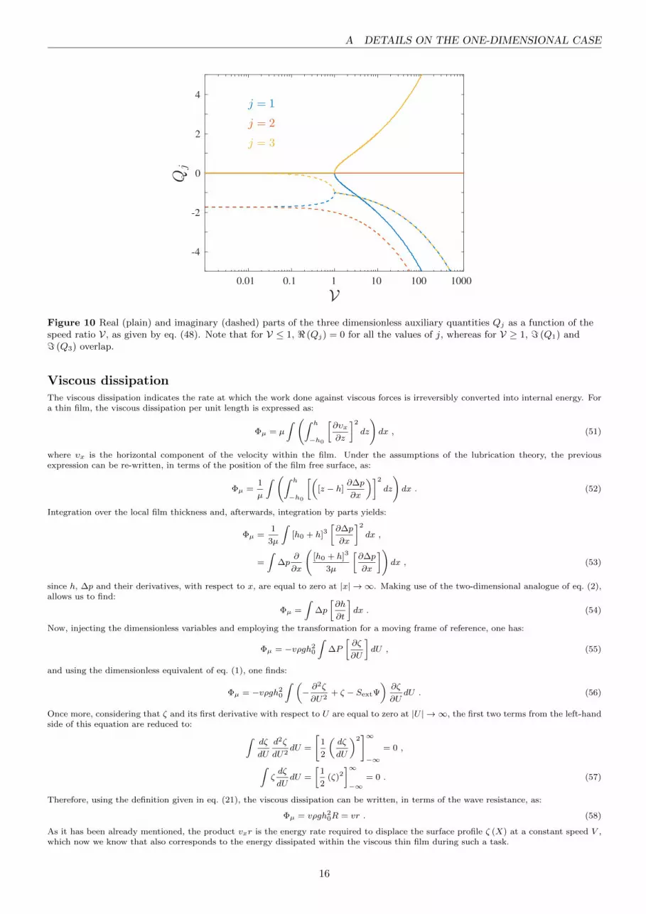
Rδ =i3√

3S2extV

2 [q1 + q2] [q1 + q3] [q2 + q3], (47)

where i =√−1 is the imaginary unit, and where we introduced the auxiliary quantities q1, q2 and q3, which are related to the roots of

V 2 +Q2[Q2 + 1

]2, as given by (see Fig. 10):

qj =

[θ

σj

]1/2−[σjθ

]1/2,

θ =(

1− 2V2 + 2V√V2 − 1

)1/3, (48)

and σj has been introduced in eq. (17). After some math, one is able to regain eq. (26).From the substitution of a Lorentzian distribution into eq. (22) and after integration, the following expression of the wave resistance

is obtained:

RL =S2extV

2π

3∑j=−3j 6=0

Qj

1 + 4Q2j + 3Q4

j

∫ ∞0

− exp (−w)

w − 2Qj√Bo

dw , (49)

where Qj is the jth root of V 2 +Q2[Q2 + 1

]2, given by:

Qj =1√

3

[θ

σj+σj

θ− 2

]1/2, (50)

for j = 1, 2, 3, whereas for j = 4, 5, 6 Qj = −Qk where k = j − 3. σj and θ have been introduced in eqs. (17) and (48), respectively. Theasymptotic behaviours for V →∞ can be also obtained from eq. (49), after making θ → 1 and some tedious math.

15

A DETAILS ON THE ONE-DIMENSIONAL CASE

V

0.01 0.1 1 10 100 1000

Qj

-4

-2

0

2

4j = 1

j = 2

j = 3

Figure 10 Real (plain) and imaginary (dashed) parts of the three dimensionless auxiliary quantities Qj as a function of thespeed ratio V, as given by eq. (48). Note that for V ≤ 1, < (Qj) = 0 for all the values of j, whereas for V ≥ 1, = (Q1) and= (Q3) overlap.

Viscous dissipationThe viscous dissipation indicates the rate at which the work done against viscous forces is irreversibly converted into internal energy. Fora thin film, the viscous dissipation per unit length is expressed as:

Φµ = µ

∫ (∫ h

−h0

[∂υx

∂z

]2dz

)dx , (51)

where υx is the horizontal component of the velocity within the film. Under the assumptions of the lubrication theory, the previousexpression can be re-written, in terms of the position of the film free surface, as:

Φµ =1

µ

∫ (∫ h

−h0

[([z − h]

∂∆p

∂x

)]2dz

)dx . (52)

Integration over the local film thickness and, afterwards, integration by parts yields:

Φµ =1

3µ

∫[h0 + h]3

[∂∆p

∂x

]2dx ,

=

∫∆p

∂

∂x

([h0 + h]3

3µ

[∂∆p

∂x

])dx , (53)

since h, ∆p and their derivatives, with respect to x, are equal to zero at |x| → ∞. Making use of the two-dimensional analogue of eq. (2),allows us to find:

Φµ =

∫∆p

[∂h

∂t

]dx . (54)

Now, injecting the dimensionless variables and employing the transformation for a moving frame of reference, one has:

Φµ = −vρgh20∫

∆P

[∂ζ

∂U

]dU , (55)

and using the dimensionless equivalent of eq. (1), one finds:

Φµ = −vρgh20∫ (−∂2ζ

∂U2+ ζ − SextΨ

)∂ζ

∂UdU . (56)

Once more, considering that ζ and its first derivative with respect to U are equal to zero at |U | → ∞, the first two terms from the left-handside of this equation are reduced to: ∫

dζ

dU

d2ζ

dU2dU =

[1

2

(dζ

dU

)2]∞−∞

= 0 ,

∫ζdζ

dUdU =

[1

2(ζ)2

]∞−∞

= 0 . (57)

Therefore, using the definition given in eq. (21), the viscous dissipation can be written, in terms of the wave resistance, as:

Φµ = vρgh20R = vr . (58)

As it has been already mentioned, the product vxr is the energy rate required to displace the surface profile ζ (X) at a constant speed V ,which now we know that also corresponds to the energy dissipated within the viscous thin film during such a task.

16

B DETAILS ON THE TWO-DIMENSIONAL CASE

B Details on the two-dimensional case

Fourier transform

f (Q,K) =

∫ ∞−∞

∫ ∞−∞

f (U, Y ) exp (−i [QU +KY ]) dY dU ,

f (U, Y ) =1

4π2

∫ ∞−∞

∫ ∞−∞

f (Q,K) exp (i [QU +KY ]) dKdQ , (59)

Wave resistanceStarting from eq. (35), one should consider a transformation into the polar coordinates (%, ϕ), given by the relations Q = % cos (ϕ) andK = % sin (ϕ), and multiply both numerator and denominator by i/V , in order to retrieve the following expression:

R =S2ext

4π2V

∫ ∞0

∫ 2π

0

%3 cos (ϕ) Ψ (%, ϕ) Ψ (%, ϕ+ π)

cos (ϕ) + i%

V[%2 + 1]

dϕd% . (60)

Additionally, if the pressure field Ψ (%) under consideration is axisymmetric, a first integration of the previous equation over ϕ leads directly

to eq. (36). In brief, for an axisymmetric pressure field Ψ (%), we should use the following formula:∫ 2π

0

cos(ϕ)dϕ

cos(ϕ) +D= 2

∫ π

0

cos(ϕ)dϕ

cos(ϕ) +D,

= 2

2D√

1−D2tanh−1

[D − 1] tan(ϕ

2

)√

1−D2

+ ϕ

π

0

,

which, considering that:

limx→∞

[tanh−1 (x)

]=iπ

2,

can be re-written as: ∫ 2π

0

cos(ϕ)dϕ

cos(ϕ) +D= 2π

[1 +

iD√

1−D2

],

in order to perform the aforementioned integration step. Moreover, a series expansion of the integrand in eq. (36) near V = 0 leads to:

R0 =S2extV

2π

(∫ ∞0

[Ψ (%)

]2 %d%

2 [%2 + 1]2+O

(V 2))

, (61)

which can be re-write in the form of eq. (37).For a Dirac pressure distribution, eq. (36) becomes:

Rδ =S2ext

2πV

∫ ∞0

1−%[%2 + 1

]√V 2 + %2 [%2 + 1]2

%3d% . (62)

A series expansion near V = 0 of the integrand yields:

Rδ =S2extV

2π

(∫ ∞0

%d%

2 [%2 + 1]2+O

(V 2))

, (63)

which after integration is equal to:

Rδ =S2extV

8π

[1 +O

(V 2)]

. (64)

Now, using the change of variables w = %[%2 + 1

]/V and a series expansion of the integrand at V → ∞, the integral in eq. (62) can

be approximated with:

∫ ∞0

1−%[%2 + 1

]√V 2 + %2 [%2 + 1]2

%3 =V 4/3

3

∫ ∞0

w1/3

(1−

w√

1 + w2

)+O

(V 1/3

),

=

Γ

(1

3

)Γ

(7

6

)4√π

V 4/3 +O(V 1/3

),

which allows us to write down eq. (40).

17