Voronoi Cell Patterns: theoretical model and applications

Diego Luis Gonzalez∗ and T. L. Einstein†

Department of Physics, University of Maryland, College Park, Maryland 20742-4111 USA(Dated: November 29, 2011)

We use a simple fragmentation model to describe the statistical behavior of the Voronoi cellpatterns generated by a homogeneous and isotropic set of points in 1D and in 2D. In particular, weare interested in the distribution of sizes of these Voronoi cells. Our model is completely definedby two probability distributions in 1D and again in 2D, the probability to add a new point insidean existing cell and the probability that this new point is at a particular position relative to thepreexisting point inside this cell. In 1D the first distribution depends on a single parameter while thesecond distribution is defined through a fragmentation kernel; in 2D both distributions depend ona single parameter. The fragmentation kernel and the control parameters are closely related to thephysical properties of the specific system under study. We use our model to describe the Voronoi cellpatterns of several systems. Specifically, we study the island nucleation with irreversible attachment,the 1D car-parking problem, the formation of second-level administrative divisions, and the patternformed by the Paris Metro stations.

PACS numbers: 89.75.Kd,68.55.A-,05.40.-a,81.16.Rf

I. INTRODUCTION

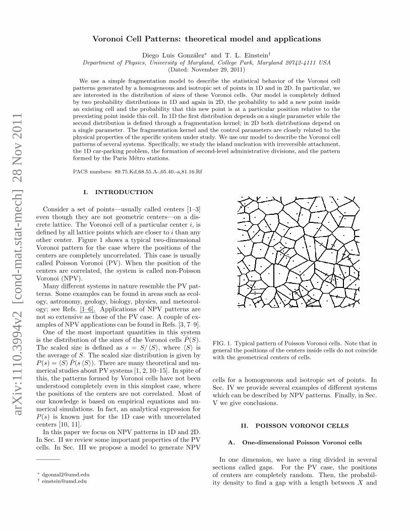
Consider a set of points—usually called centers [1–3]even though they are not geometric centers—on a dis-crete lattice. The Voronoi cell of a particular center i, isdefined by all lattice points which are closer to i than anyother center. Figure 1 shows a typical two-dimensionalVoronoi pattern for the case where the positions of thecenters are completely uncorrelated. This case is usuallycalled Poisson Voronoi (PV). When the position of thecenters are correlated, the system is called non-PoissonVoronoi (NPV).

Many different systems in nature resemble the PV pat-terns. Some examples can be found in areas such as ecol-ogy, astronomy, geology, biology, physics, and meteorol-ogy; see Refs. [1–6]. Applications of NPV patterns arenot so extensive as those of the PV case. A couple of ex-amples of NPV applications can be found in Refs. [3, 7–9].

One of the most important quantities in this systemis the distribution of the sizes of the Voronoi cells P (S).The scaled size is defined as s = S/ 〈S〉, where 〈S〉 isthe average of S. The scaled size distribution is given byP (s) = 〈S〉 P (s 〈S〉). There are many theoretical and nu-merical studies about PV systems [1, 2, 10–15]. In spite ofthis, the patterns formed by Voronoi cells have not beenunderstood completely even in this simplest case, wherethe positions of the centers are not correlated. Most ofour knowledge is based on empirical equations and nu-merical simulations. In fact, an analytical expression forP (s) is known just for the 1D case with uncorrelatedcenters [10, 11].

In this paper we focus on NPV patterns in 1D and 2D.In Sec. II we review some important properties of the PVcells. In Sec. III we propose a model to generate NPV

∗ dgonzal2@umd.edu† einstein@umd.edu

FIG. 1. Typical pattern of Poisson Voronoi cells. Note that ingeneral the positions of the centers inside cells do not coincidewith the geometrical centers of cells.

cells for a homogeneous and isotropic set of points. InSec. IV we provide several examples of different systemswhich can be described by NPV patterns. Finally, in Sec.V we give conclusions.

II. POISSON VORONOI CELLS

A. One-dimensional Poisson Voronoi cells

In one dimension, we have a ring divided in severalsections called gaps. For the PV case, the positionsof centers are completely random. Then, the probabil-ity density to find a gap with a length between X and

arX

iv:1

110.

3994

v2 [

cond

-mat

.sta

t-m

ech]

28

Nov

201

1

2

X + dX, p(0)(X), is given by ρ e−ρX , where ρ is thedensity of centers. The normalized gap size is definedas x = X/〈X〉 where 〈X〉 = ρ−1 is the average gap size.Thus, the normalized gap size distribution can be writtenas p(0)(s) = e−x. By definition, p(n)(x) is the probabil-ity density to find a gap which starts and ends with acenter subject to the condition that there are n addi-tional centers inside the gap. These distributions sat-isfy the normalization conditions

∫∞0

dx p(n)(x) = 1 and∫∞0

dxx p(n)(x) = n + 1. Because sizes of the adjacentgaps are not correlated, it is possible to write the nor-malized spacing distributions for arbitrary values of n inLaplace space as

p(n)(l) =(p(0)(l)

)n+1

, (1)

where p(n)(l) =∫∞

0dx e−x l p(n)(x) is the Laplace trans-

form of p(n)(x) [16]. Consequently, the normalized spac-ing distributions between centers are given by

p(n)(x) =1

n!xne−x. (2)

The pair correlation function has the simple form

g(x) =

∞∑n=0

p(n)(x) = 1. (3)

The size distribution of the Vononoi cells is related to thenext-nearest-neighbor distribution according to [8]

P (s) = 2 p(1)(2s). (4)

This equation is a consequence of the one-dimensional na-ture of the ring. Therefore, the simple relation betweenP (s) and p(1)(s) shown above is not valid for higher di-mensions. Explicitly, the distribution of sizes of Voronoicells in 1D is

P (s) = 4 s e−2 s. (5)

B. Two-dimensional Poisson Voronoi cells

Let p(n)(R) be the radial probability density that,given an island at r = 0, its (n + 1)th neighbor is be-tween R and R + dR. Given that there are n additionalcenters inside of the circle of radius R, the radial spacingdistribution, p(n)(R), can be calculated as follows. Asusual, ρ is the density of centers. On average, the totalnumber of centers, c(R), within a disk with radius R is2πρR. It is well known [19] that c(R) and p(0)(R) arerelated by

p(0)(R) = c(R)e−∫R0dr 2πr c(r). (6)

More details about this equation are given in the Ap-pendix. Since c(R) = 2π Rρ, p(0)(R) has the simpleform

p(0)(R) = 2π ρR e−π ρR2

. (7)

The next radial distribution p(1)(R) is given by

p(1)(R) = 2π ρR

∫ R

0

dR′ p(0)(R′)Q(R′, R), (8)

where Q(R′, R) = e−π ρ(R2−R′2) is the probability density

to have the annulus R′ ≤ r ≤ R free of centers. Theintegral in Eq. (8) can be calculated straightforwardly togive

p(1)(R) = 2π2 ρ2R3e−π ρR2

. (9)

Following the previous procedure, one can show that, forarbitrary n,

p(n)(R) = 2(π ρ)n+1

n!R2n+1e−π ρR

2

. (10)

As for multineighbor spacing distributions in 1D [16–18], the radial distributions have information about thestructure of the system. For example, since

2π Rρ g(R) =

∞∑n=0

p(n)(R), (11)

it is possible to calculate the radial distribution functiong(R). From Eqs. (10) and (11) it is easy to find

g(R) = e−π ρR2∞∑n=0

(π ρR2)n

n!= 1. (12)

This result is consistent with this case of uncorrelatedcenters g(R) = 1. In general the concentration of centersc(R) can be extracted from p(0)(R). From Eq. (6) itfollows

c(R) =p(0)(R)∫∞

Rdrp(0)(r)

. (13)

Even though we know the exact expression for the ra-dial spacing distributions for arbitrary values of n in thePV case, the exact functional form of P (s) is not knownfor d ≥ 2. In fact, just a few exact analytical results areknown in this case. One of them was reported in 1962by Gilbert [15], who showed that the second moment ofP (S) is 0.280〈S〉.

As mentioned previously, obtaining the exact expres-sion of P (s) for d > 1 is quite complicated partially duegeometrical complications. In d = 1 each new center di-vides just one of the existing Voronoi cells to form twonew cells. This fact leads to the simple relation betweenP (x) and p(1)(x) given by Eq. (4). In higher dimensionsthis does not apply; the Voronoi cell of a new centeris formed at the expense of several preexisting Voronoicells. An analogous relation to Eq. (4) for d > 1 remainsunknown, and it could involve several p(n)(r) in a non-trivial way. However, it is well accepted that P (s) can beapproximated by the gamma distribution Πα(s). Based

3

FIG. 2. (Color online) Poisson Voronoi cell-size distributionP (s) with d = 2. The agreement between the numerical re-sults and Eq. (14) is excellent. The inset shows the radial dis-

tribution functions p(n)(r). Red lines correspond to Eqs. (10)and (14).

on extensive numerical simulations for d = 1, 2, 3, Ferencand Neda [11] proposed

P (s) ≈ Πα(s) =αα

Γ(α)sα−1e−α s (14)

where α = (3d+1)/2. Note that for d = 1 we recoverEq. (5). The agreement between Eq. (14) and the nu-merical results for P (s) is excellent, as seen in Fig. 2.

III. NON-POISSONIAN VORONOI CELLS

More complicate behavior arises when the centers arecorrelated in some way. Although there are few stud-ies [3, 7–9] about such systems, the NPV patterns canbe used to describe qualitatively and quantitative manydifferent systems, as we shall see.

A. One-dimensional non-Poissonian Voronoi cells

To generate a one-dimensional NPV set of centers weproceed as follows. Let pg(x) be the probability densityto put a new center inside a gap with a scaled size x.In a similar way, px(x) is the probability density thatthe new center is placed at the position x with respectto the center at the left of the gap. This kind of modelproved fruitful in studying the spatial structure of theone-dimensional point-island model for epitaxial growth.In fact, a suitable choice of pg(x) and px(x) leads to anexcellent description of the physical properties of this sys-tem [8, 9]. The gap size distribution, p(0)(x), was shown

there to satisfy the equation

xdp(0)(x)

dx+ 2 p(0)(x) = −pg(x) + 2 px(x), (15)

In particular, the probability to put a new center insidea gap has the form

pg(x) =xγ

µγp(0)(x), (16)

with µγ the γth moment of p(0)(x). The probability den-sity px(x) can be written as

px(x) =

∫ ∞x

dz1

zpg(z)pΛ(x/z), (17)

where pΛ(x/z)dx/z is the conditional probability that,given a particular gap with size z, the new center isplaced inside [x, x + dx]. Unfortunately, in most casesthe integro-differential given by Eqs. (15), (16) and (17)cannot be solved analytically. However, this system canbe simulated numerically without major difficulties [20].

Nonetheless, some exact results can be extracted fromEq. (15). If we choose γ = 1 and pΛ(λ = x/z) = 1, theprobability to put a new center onto an empty site is thesame for all empty sites on the lattice. Then, with thisselection of γ and pΛ(λ), we recover the one-dimensionalPV case discussed previously in Sec. II-A. As mentioned,the position of the centers in the PV case are totallyuncorrelated, and p(n)(x) is given by Eq. (2), while P (s)is given by Eq. (5).

In general, for γ ≥ 1 and pΛ(x/z) = 1, the solution ofEq. (15) can be calculated as follows. The simple form ofthe kernel pΛ(λ) leads to dpx(x)/dx = −xγ−1p(0)(x)/µγ .Then, differentiating Eq. (15) we have

xd2p(0)(x)

dx2+

(3 +

xγ

µγ

)dpx(x)

dx+(2 + γ)

xγ−1

µγp(0)(x) = 0.

(18)After some algebra the above equation can be written as(

d

dx+

2

x

)(xdp(0)(x)

dx+xγ

µγp(0)(x)

)= 0, (19)

whose general solution is

p(0)(x) =1

Γ(

1 + 1γ

)(µγ γ)

1γ

e− xγ

γ µγ , (20)

with µγ = [Γ(1/γ)/Γ(2/γ)]γ/γ. In this case px(x) is also

given by Eq. (20). Note that p(0)(0) 6= 0. For this casehigher spacing distributions, in particular P (s), cannotbe calculated easily.

Consider now a more general case where pΛ(x/z) de-pends on x and z. We restrict our work to functionswhich are symmetrical about λ = x/z = 1/2. This sym-metry property comes from the fact that in the absenceof an external drift (e.g., a field), pΛ(1 − x/z) must be

4

equal to pΛ(x/z). Furthermore, we impose the additionalcondition pΛ(0) = pΛ(1) = 0. This property implies thatthe probability to place a new center near an existing oneis small.

For large values of x, dp(0)(x)/dx is negative. Then,in this regime the behavior of p(0)(x) is dominated bypg(x). Consequently, for x� 1, Eq. (15) takes the form

xdp(0)(x)

dx≈ −x

γ

µγp(0)(x), (21)

which implies p(0)(x) ∝ exp (−xγ/(γ µγ)) and p(0)(x) �px(x). A first correction to this formula can be obtainedby using the ansatz p(0)(x) ∝ f(x) exp (−xγ/(γ µγ)) inEq. (15). This procedure gives the differential equation

xdf(x)

dx+ 2 f(x) = 0. (22)

We conclude that p(0)(x) ∝ x−2exp (−xγ/(γ µγ)). Then

the behavior of p(0)(x) for large values of x is completelydetermined by the parameter γ. Furthermore, in thelimit x� 1 the solution of Eq. (15) does not depend onpΛ(λ). However, pΛ(λ) controls the behavior of p(0)(x)for small values of x. In general, for the kind of func-tions considered here, for λ � 1 we have pΛ(λ) ∼ λζ ,with ζ a constant which depends on the functional formof pΛ(λ). A series expansion of Eqs. (15) and (17) showsthat p(0)(x) ∼ xζ and px(x) ∼ xζ . It is clear that thevanishing condition imposed on pΛ(λ) for λ = 0 leadsto p(0)(0) = 0. The effective entropic “repulsion force”between centers is determined by the parameter ζ givenby the series expansion of pΛ(λ) around λ = 0.

B. Two-dimensional non-Poissonian Voronoi cells

In the case d = 2 we proceed as follows. Let qc(s)be the probability density to put a new center within aVoronoi cell having a scaled area s. Explicitly, we con-sider the general form

qc(s) =sγ

µγP (s), (23)

where µγ is the γth moment of P (s). In a similar way,we define qr(r, s) as the probability density that, for aparticular cell with scaled size s, the new center is lo-cated at a position r with respect to the center of thepreexisting cell. For the sake of simplicity, we considerjust the isotropic case where (with r ≡ |r|)

qr(r, s) ∼ rδ. (24)

In this simplification, the probability to put a new centerinside a cell depends on the cell itself, regardless of thepositions of neighboring centers or the areas of their sur-rounding cells. The functional form of qr(r, s) depends

on the shape of the Voronoi cell. For example, in the caseof a circular Voronoi cell with scaled area s, we have

qr(r, s) =δ + 2

2 s1+ δ2

πδ2 rδ. (25)

The simplest case is γ = 1 and δ = 0, for which qr(r, s) ∝1/s. In this case every empty point of the lattice has thesame probability to receive a new center. This, of course,corresponds to the PV case discussed in Sec. II-B andshown in Fig. 2.

From a Taylor expansion of Eq. (6) around R = 0,it is clear that the behavior of p(0)(R) is controlled bythe functional form of c(R). For small values of R, it isreasonable to suppose that the concentration of particleswithin a distance R and R + dR from a given centeris proportional to the product of qr(R, s) and the areadA = 2π RdR; then

c(R) dR ∼ qr(R, s) dA ∼ Rδ+1dR. (26)

Then, p(0)(R) ∼ Rδ+1, and δ controls the effective “re-pulsion force” between centers. Using this simple resultin Eq. (11) we conclude that, for R� 1, g(R) ∼ Rδ. Onthe other hand, the behavior of p(0)(R) for large values

of R depends on the behavior of the integral∫ R

0dξ c(ξ).

The equivalent of Eq. (15) for the 2D case cannot bewritten easily in terms of known quantities. FollowingRef. [21], the effect of a new center on P (s) can be writtenas

sdP (s)

ds+ 2P (s) = M p+(s)−M pA(s) + p∗(s), (27)

where M is the average number of preexisting Voronoicells overlapped by the Voronoi cell generated by the newcenter; p+(s) is the probability density that the new cen-ter reduces the Voronoi cell size of a preexisting cell tos, pA(s) is the probability density that the Voronoi cellof the new center overlaps a preexisting cell with size s;and p∗(s) is the probability density that the new Voronoicell has size s.

From their definitions, qc(s) and pA(s) are clearlyrelated: qc(s) takes into account the destruction of a

(a) (b)

FIG. 3. In (a) is the initial configuration of centers, while in(b) the effect of a new center on the preexisting Voronoi cellsis shown. Note that in this particular case, the new Voronoicell is almost completely defined by the first three neighborsof the new center.

5

Voronoi cell by the direct impact of a new center onthat cell, while pA(s) is more general and expresses thatthe Voronoi cell of a new center overlaps on averageM preexisting Voronoi cells. Then we can expect thatpA(s) ∼ qc(s) ∼ sγP (s). On the other hand, for largevalues of s, dP (s)/ds < 0, which means that pA(s) con-trols the right side of Eq. (27). Thus, in this limit wecan expect that P (s) ∼ exp (−M sγ/(γ µγ)). In our 2Dmodel, the tail of P (s) for large values of s depends onthe parameter γ.

In the opposite limit s � 1, the behavior of P (s) isgiven by p∗(s) because this distribution dominates theright side of Eq. (27). Then p∗(s) ∼ sζ implies P (s) ∼ sζ .In order to understand the behavior of p∗(s) for smallvalues of s we proceed as follows.

In the simplest case a new Voronoi cell is completelydefined by just three nearby centers; see Fig. 3. Notethat the new center shown in Fig. 3(b) generates a smallVoronoi cell even though it was formed at the expenseof the three large Voronoi cells shown in Fig. 3(a). If pcis the probability to have the initial configuration shownin Fig. 3(a), then the probability to place a new centeras in Fig. 3(b) is given by pcA

γ where A is the area ofthe target region. Naturally, A scales with the distancebetween centers as A ∼ r2. In the case of noncorre-lated centers, pc ∼ p(0)(r1)p(0)(r2 − r1)p(0)(r3 − r2) ∼c(r1)c(r2 − r1)c(r3 − r2) which leads to pc ∼ r3. In thePV case we have γ = 1; thus, p∗(s) ∼ s2.5. Note thatthis result agrees with Eq. (14). The case of correlatedcenters is significantly more complicated because pc can-not be written as an independent product of p(0)(s). Inany case, it is clear that p∗(s) for small values of s is re-lated with the concentration of centers c(R) through theradial distribution functions which in turn in our modeldepend on δ. Then, the value of ζ in P (s) ∼ sζ for agiven value of γ increases with δ. However, a generalrelation between δ and ζ remains unknown.

As noted, Eq. (27) cannot be solved analytically; how-ever, the numerical simulation of this system can be donewithout major complications [22].

IV. APPLICATIONS OF THE NPV PATTERNS

A. Gap size distribution of parked cars

Rawal and Rodgers (RR hereafter) measured the sizeof the gaps between adjacent parked cars [23]. The data(500 gaps) were gathered from four connected streets inLondon without any side streets or driveways. Theyfound that small and large gaps are unlikely. The ef-fective repulsion between adjacent cars arises becausedrivers need to leave some space between cars to allowexit maneuvers. RR suggest that large gaps are unlikelybecause people try avoid the waste of space. However, webelieve that it is more reasonable to think that this hap-pens because people usually prefer to park in large gapswhere the entry maneuver is the easiest. This implies

FIG. 4. (Color online) NPV case with γ = 4 and pΛ(λ) =2 sin2(πλ). Here empirical data A and B correspond to themeasurements reported in Refs. [23] and [25], respectively.

that large gaps are often destroyed before small ones.RR developed two different models to describe p(0)(x);however, just one of them describes the statistical be-havior of the system properly. In their improved modelthey consider two different factors: people who park any-where and those who perform an additional maneuver toavoid the waste of space. These assumptions give a gooddescription of the empirical data.

On the other hand, Abul-Magd [24] used the Wignersurmise (WS) with β = 2 as an approximate model forp(0)(x). The WS describes the gap distribution of a one-dimensional Coulomb gas at an inverse temperature β.In this system, particles are free to move around a circlebut experience a logarithmic potential interaction. Heselected this value of the inverse temperature β becausein this case the WS describes excellently the statisticalbehavior of chaotic systems without time-reversal sym-metry, as is appropriate for the car-parking problem. TheWS does give a good quantitative description of the car-parking problem; however, the physical interpretation ofthe logarithmic interaction potential among cars is notentirely clear. In Ref. [25], Seba reported more exten-sive (over 1200 gaps) empirical data for the gap sizes.He modeled the car parking with a Markov chain wherethe cars are allowed to get in and get out of the gapsfollowing prescribed probabilistic rules.

From our model to generate one-dimensional Voronoicells, we can interpret the car-parking problem more sim-ply and intuitively. As in the models mentioned before,our NPV model for car parking contains some simplify-ing assumptions for an ensemble of drivers such as homo-geneity and isotropy. Our goal is to analyze a tractableversion for the problem rather than contend with all thesubtleties. As mentioned previously, we start with the as-sumption that people prefer to park in large gaps rather

6

than in small ones. This follows from the fact that theparallel parking is easier in spots where there is space tospare. Thus, it is reasonable to propose that the prob-ability to park in a gap with size x can be modeled byEq. (16). Naturally we have to choose the appropriatevalue of γ. Once the gap has been selected, the driverhas to choose the exact parking place inside the gap. Forgaps shorter than two car lengths the most likely placeto park would seem to be the middle of the gap. For lackof a better simple ansatz, we extend this assumption togaps of arbitrary length. Additionally, the driver shouldavoid parking too close to the cars on the borders of thegap in order to guarantee enough space to leave the gapwhen necessary. This implies pΛ(0) = pΛ(1) = 0. Fi-nally, we claim that pΛ(λ) = pΛ(1 − λ); i.e., the driversdo not have preference to park near to the car on eitherside of the gap. A simple function which satisfies thoseproperties is pΛ(λ) = 2 sin2(πλ). From our numericalresults we found this functional form for pΛ(λ) gives areasonable description of the empirical data when γ = 4.

As shown in Fig. 4, our model describes excellently theempirical data given in Refs. [23, 25]. Of course, morerefined models can be developed, but the most importantresult is that a suitable selection of γ and pΛ(λ) leads toan excellent description and interpretation of the statis-tical behavior of the gap size of parked cars. From ourprevious discussion, it is clear that p(0)(x) ∼ xζ withζ = 2 for x � 1. The value of ζ is related to the ef-fective “repulsion force” between adjacent cars. In thelimit x � 1, p(0)(x) ∼ x2 exp(−x4/(4µγ)). Note thatγ = 4 represents the strong preference of drivers to parkin large gaps rather than in small ones.

In the problem of parked cars, we can interpret theVoronoi size distribution P (s) through the next-nearestspacing distribution p(1)(x) as follows. From its defini-tion, p(1)(x) clearly gives the probability density that aparked car has a spot of length x to perform the exitmaneuver. From Eq. (4), the distribution of the Voronoicell sizes s is proportional to the distribution of distancesx that the drivers have to perform an exit maneuver.

B. Point-island model for epitaxial growth in 1Dand 2D

In the point-island model for epitaxial growth, atomsare deposited onto a substrate where they perform ran-dom walks. In the simplest case, when two atoms meetthey form a static island. In the same way, the atomswhich reach an island are captured and remain attachedto it. This case corresponds to irreversible attachmentand is usually called “i = 1” in the literature. Anotherimportant characteristic of the point-island model is thefact that the islands do not grow laterally. The size ofa particular island is given just by the number of atomswhich belong to it. This system exhibits a scaling regimein the limit < = F/D → ∞, where F is the depositionrate of atoms and D is their diffusion constant. This

model is, of course, a simplification of the real systembut it contains most of the relevant physical propertiesrequired to describe the processes behind the island for-mation in epitaxial growth [8, 9, 21, 26, 29–32]. In fact,the widely used point-island model gives very accurateresults in early stages of growth (low coverages) and it isan important theoretical model in our knowledge aboutepitaxial growth.

In this context, the point islands determine the patternof Vononoi cells, playing the role of the centers definedin Sec. I. The atoms inside a particular Voronoi cellare usually captured by the center of the cell (island).Because of this, the Voronoi cells are called capture zones(CZs) in the context of epitaxial growth. Naturally, thegrowth rate of an island is related to the size of its CZ.For more details about these kinds of models see, forexamples, Refs. [8, 9, 26–34].

1. One-dimensional case

Consider now the case of a one-dimensional substratewith irreversible attachment. A suitable choice to de-scribe the spacing and the CZ distributions of the 1Dpoint-island model is [8]

pΛ(λ) = 30λ2(1− λ)2 (28)

and

γ(x) =

{3, if x > 1.74, if x ≤ 1.7

(29)

Blackman and Mulheran [9] originally calculatedEq. (28) by first obtaining the average density of atoms,n1(x, y), inside a gap of length y from its expression inthe stationary state. From this approximation and as-suming that the probability of a new nucleation at x isproportional to n1(x, y)2, they found Eq. (28). On theother hand, Eq. (29) is based on the numerical results re-ported in Ref. [8]. In Fig. 5(a), the results of this modelare shown and compared with the direct numerical sim-ulation of the island nucleation for three different valuesof <; the agreement is excellent. This selection of γ(x)and pΛ(λ) reproduce the statistical behavior of the 1Dpoint-island model with irreversible attachment. For ad-ditional information see Refs. [8, 9].

2. 2D in circular-cell approximation

The point-island model with irreversible attachment intwo dimensions can be modeled following a similar proce-dure to that was used previously to described nucleationin one dimension. To make analytic progress, we followRefs. [35–38] by approximating the Voronoi cells as circu-lar. (While Figs. 1, 3, etc., show that typical cells are farfrom circular, the approximation is better than might beanticipated because the average shape over an ensemble

7

(a) (b)

FIG. 5. (Color online) The statistical behavior of irreversible nucleation in 1D is shown in (a). The CZ distribution for 2Dnucleation is shown in (b). In all cases our results are compared with direct numerical simulations of island nucleation forseveral values of <.

FIG. 6. (Color online) Behavior of the first radial distribution

p(0)(r), which is related to the concentration of islands c(r).

of cells does tend toward circular.) As shown in Eq. (B2a)of Ref. [35] and Eq. (9) of Ref. [38], the isotropic steady-state solution of the appropriate diffusion equation withflux F inside such a circular Voronoi cell with radius Rc,for a concentric (non-point) island of radius Risl < Rc,gives the following expression for the density of atoms:

ρ(R) =1

2

R2c

<

[ln

(R

Risl

)+

1

2

R2isl

R2c

(1− R2

R2isl

)], (30)

where R (assuming Risl ≤ R ≤ Rc) is the distance fromthe cell center. Note that ρ(Risl) = 0 (thence increasinglinearly with R − Risl initially) and dρ(R)/dR|Rc = 0.The first condition comes from the density of atoms beingzero along the island boundaries. On the other hand, theprobability of nucleation is proportional to ρ2(R), whichis maximal along the boundary of the CZ. Hence, ρ(R)

is also maximal at R = Rc, as implied in the second(Neumann) condition.

In this framework [with nucleation ∝ ρ2(R)], the prob-ability to have a nucleation event within a particular cir-cular capture zone with radius Rc, Pn(Rs), can be writ-ten as

Pn(S) =qγ(S)

P (S)∝∫ Rc

Risl

dR 2π Rρ2(R) ∝ R6c . (31)

Note that Pn(S) is proportional to the third power of thescaled area of the cell, i.e., γ = 3. This is, of course, astrong approximation. It is well known that the radiusof a capture zone fluctuates significantly around its meanvalue because the centers are usually not at the geometriccenter of the cells. Approximating the shape of a CZ bya circle neglects those radial fluctuations. Furthermore,the density of atoms inside a CZ depends on the positionof neighboring centers, which is not taken into accountby Eq. (30). This also implies that the isotropy assump-tion used to write Eq. (24) is poor. From Eq. (31) it isclear that the probability of nucleation increases with thedistance from the center and reaches its maximum alongthe boundary of the capture zone. There are many waysto select the place of nucleation inside a particular cap-ture zone [36–38]. However, in order to keep our modelas simple as possible, we assign the same probability toall points inside a particular CZ, regardless of their dis-tance from the center; i.e., α = 0. While this is a crudeapproximation, we can see in Fig. 5 that it is adequateto describe P (s). However, previous simplifications haveimportant effects on the radial distributions. Figure 6shows the behavior of p(0)(r). Not unexpectedly, oursimplified model does not describe p(0)(r) appropriately;i.e., it is not a good approximation for the island densityc(R). From Eq. (30) it is clear that the concentration ofislands in the limit R � 1 is given by c(r) ∼ R2, whichimplies δ = 1.

8

In order to improve our model, we must take into ac-count the fact that ρ(R) vanishes along the boundaries ofthe islands; i.e., qr(0, s) = 0. Perhaps the simplest wayto accomplish this goal for the point-island model is topropose

qr(R, s) ∼{

R, if 0 ≤ R ≤ κRcκRc, if κRc < R ≤ Rc

(32)

where 0 < κ < 1 is a constant, and Rc = (S/π)1/2 is theaverage radius of the CZ. From our numerical experimen-tation we estimate κ = 0.3. In this way, the nucleationprobability inside a capture zone grows linearly with Rfor points near the island, while it becomes constant forpoints far away.

Figures 5(b) and 6 also include the results of this lastmodel. The description of P (s) is again excellent, butnow the nearest-neighbor radial distribution is also wellfitted. Thus, in our model for the island nucleation in 2D,the repulsion between centers given by α seemingly hasa great impact on p(0)(r) but is not crucial to determineP (s).

C. Size distribution of second-level administrativedivisions

The polygons formed by county boundaries in the size-division model resemble Voronoi cells [6, 39]. Inspiredby this fact, we explore the possibility to use our NPVmodel to study the formation of second-level administra-tive divisions (SLADs), such as counties in the USA or(non-urban) districts (arrondissements) in France. Theformation of SLADs depends on many political, cultural,ecological, and geographical factors [6, 40]. These fac-tors are in general difficult to include in a mathematicalmodel. However, our model allows us to give a simpleinterpretation of the SLAD formation in terms of qc(s)and qr(r, s).

We focus here on the results reported by Le Caer andDelannay (LCD) for the SLADs in France [6]. The de-partments (departements) comprise the first administra-tive division in France. In mainland France there are 94departments. Each department is divided into severaldistricts; there are a total of 322 districts in mainlandFrance. Each district has a chief town, mostly with thesame name as the district.

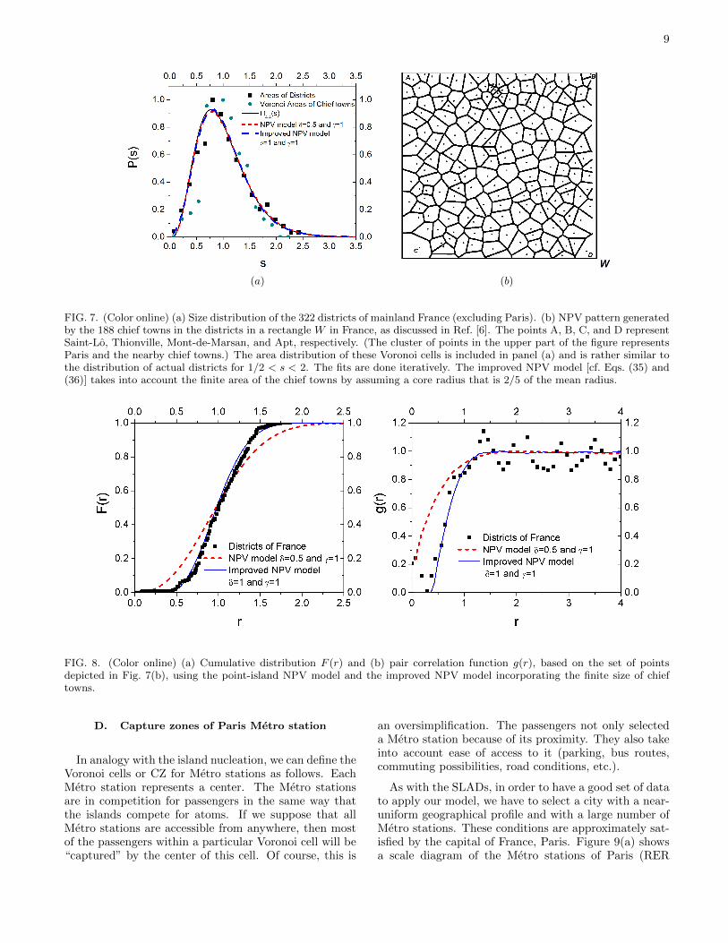
LCD compared the area distribution of the FrenchSLADs [6, 42] to the one-parameter gamma distributionΠα(s) with α ≈ 4.4 [43]. As seen in Fig. 7(a), the agree-ment between Π4.4(s) and the data is satisfactory. Notethat α = 4.4 is larger than the value used to describethe size distribution of PV cells (α = 2.5). In our model,this implies δ > 0. It follows that the SLAD formationprocess in the rectangle W was not a completely randomprocess. In fact, taking δ = 0.5 and γ = 1 we foundgood agreement between the data and the results of ourmodel. The value of γ was chosen to have an exponentialtail for P (s) such as in Eq. (14).

In particular LCD focused on the pattern formed bythe chief towns of the districts which are located withina 544 km × 636 km rectangle whose corners are closeto the towns Saint-Lo, Thionville, Apt, and Mont-de-Marsan. The average distance between the enclosed 188chief towns is 29.6 km. As shown in Fig. 7(b), the patternformed by the chief towns looks similar to that in Fig. 1.However, as noted by LCD, the formation of these SLADswas not a PV process.

The parameters δ = 0.5 and γ = 1 do not describe thecumulative nearest-neighbor distribution,

F (r) =

∫ r

0

dξ p(0)(ξ), (33)

nor the pair correlation function,

g(r) =1

ρN

∑N

i 6=j〈δ(r + rj − ri)〉 (34)

as seen in Fig. 8. Increasing the value of δ improvesthe estimation of F (r) and g(r) but it leads to a poordescription of P (s). This means that a model like oursis insufficient for this kind of system.

We attribute this discrepancy to the assumption ofpoint islands. One must account for the actual areasof cities, which produces an effective short-range repul-sion. The simplest way to incorporate this feature intoour model is to introduce an excluded area around eachcity center in the form of a hard-core radius rcore. Inparticular, we modify Eqs. (23) and (24) as follows:

qc(s) =

(s− π r2

core

)γµγ

P (s)Θ(s− π r2core), (35)

and

qr(r, s) ∼ (r − rcore)δ Θ(r − rcore), (36)

where Θ(ξ) is the unit step function. When rcore = 0, werecover the original model. From numerical simulation ofthis improved model, we found excellent agreement withthe data by using rcore/ 〈r〉 ≈ 0.4, δ = 2, and γ = 2(see Figs. 7 and 8). This improved model still describesadequately P (s), but now the fits involving p(0)(r) andg(r) are significantly better. Note that this model doesnot describe the cluster given by Paris and the nearbytowns. Clearly, the population density is highest in Parisand its surroundings. Consequently, it is reasonable toexpect the formation of clusters of towns in this regionof France, which is inconsistent with our ansatz of anexcluded area.

Our analysis has been applied to SLADs in some20 countries, with results generally consistent with theabove analysis [41]. As we report in Ref. [41], however,there are some subtleties and a rich range of nuances,e.g., regional differences in the distributions of the areasof counties in the USA.

9

(a) (b)

FIG. 7. (Color online) (a) Size distribution of the 322 districts of mainland France (excluding Paris). (b) NPV pattern generatedby the 188 chief towns in the districts in a rectangle W in France, as discussed in Ref. [6]. The points A, B, C, and D representSaint-Lo, Thionville, Mont-de-Marsan, and Apt, respectively. (The cluster of points in the upper part of the figure representsParis and the nearby chief towns.) The area distribution of these Voronoi cells is included in panel (a) and is rather similar tothe distribution of actual districts for 1/2 < s < 2. The fits are done iteratively. The improved NPV model [cf. Eqs. (35) and(36)] takes into account the finite area of the chief towns by assuming a core radius that is 2/5 of the mean radius.

FIG. 8. (Color online) (a) Cumulative distribution F (r) and (b) pair correlation function g(r), based on the set of pointsdepicted in Fig. 7(b), using the point-island NPV model and the improved NPV model incorporating the finite size of chieftowns.

D. Capture zones of Paris Metro station

In analogy with the island nucleation, we can define theVoronoi cells or CZ for Metro stations as follows. EachMetro station represents a center. The Metro stationsare in competition for passengers in the same way thatthe islands compete for atoms. If we suppose that allMetro stations are accessible from anywhere, then mostof the passengers within a particular Voronoi cell will be“captured” by the center of this cell. Of course, this is

an oversimplification. The passengers not only selecteda Metro station because of its proximity. They also takeinto account ease of access to it (parking, bus routes,commuting possibilities, road conditions, etc.).

As with the SLADs, in order to have a good set of datato apply our model, we have to select a city with a near-uniform geographical profile and with a large number ofMetro stations. These conditions are approximately sat-isfied by the capital of France, Paris. Figure 9(a) showsa scale diagram of the Metro stations of Paris (RER

10

(a) (b)

FIG. 9. (Color online) (a) Voronoi cells (CZ) for the Paris Metro stations. The complete network of stations on the left isenlarged to show the stations and associated cells near the heart of the city. (b) Capture-zone distribution of the Paris Metrostations.

stops are also included). Clearly the density of centers(Metro stations) is not constant. Naturally, there aremore Metro stations near the center of the city, wherethe population density is highest. Because of this, thelargest Voronoi cells are near the outskirts of the city.However, we can expect that our NPV model works wellif we just consider stations near the city center, where thedensity of Metro stations does not change dramatically,as seen in the enlargement in the figure.

For economic reasons it is unlikely that two or moreMetro stations are very close together. We then expectα > 0 because there is an effective “repulsion force” be-tween stations. In Fig. 9(b), we compare the empiricalCZ distribution of the in-town Metro system with ourNPV model. Good agreement is found with γ = 2 andα = 1.5; the gamma function Π8(s) is also included inthe comparison presented in Fig. 9(b). Apparently the“repulsion force” between Metro stations is bigger thanthat for island nucleation in 2D.

V. CONCLUSIONS

Our proposed NPV model can be used to describe andinterpret many different systems in terms of two inde-pendent distribution functions. In 1D, pg(x) gives theprobability density to put a new center inside a gapwith a scaled size x. This distribution is given explic-itly by Eq. (16) and is controlled by the parameter γ.This parameter determines the behavior of the gap sizedistribution for large values of x. In fact, for x � 1,p(0)(x) ≈ Ax−2exp (−xγ/(γ µγ)), independent of thekernel pΛ(λ). Additionally, γ modulates the size depen-dence of the destruction of gaps. For γ = 0, the proba-bility to put a new center within a gap is the same for allgaps, regardless of their size. The larger γ is, the greateris the probability of destruction of large gaps. For the

car-parking problem we use γ = 4, which reflects thepreference of drivers to park in large gaps rather thansmall ones. For island nucleation in 1D it is necessary totake into account that γ is a function of the scaled sizes.

In 1D, the behavior of p(0)(s) in the limit s � 1is completely determined by the fragmentation kernelpΛ(λ). For the kernels considered here, we always havethe generic behavior pΛ(λ) ∼ λζ for λ � 1. The pa-rameter ζ controls the effective repulsion force betweencenters. For island nucleation in 1D and the car-parkingproblem, we found ζ = 2. For the first system the valueof ζ is fully determined by the density of atoms insidethe gap in the aggregation regime. In the car-parkingproblem, ζ reflects the need of the drivers of allow spacebetween cars to perform an exit maneuver.

In 2D, the probability density qc(s) to put a new cen-ter inside a Voronoi cell is also controlled by the param-eter γ. In the case of the SLADs, γ = 1 gives a goodfit of the empirical data. Because of this, the P (s) ofmany SLADs can be approximated by using the single-parameter gamma distribution Πα(s) [40]. In the case ofParis Metro stations we used γ = 2.

The position r of a new center inside a particularVoronoi cell in 2D is determined in our model throughpδ(r, s). For the sake of simplicity, we consider onlyisotropic cases. This probability is closely related to theconcentration of centers c(R). For example, in the case ofisland nucleation in two dimensions, a good descriptionof p(0)(r) requires taking into account that the density ofatoms vanishes along the island boundaries, even thoughthe CZ distribution can be well described without takinginto account this fact. This suggests that many differentfragmentation models can be used to describe the CZ dis-tribution of islands in epitaxial growth. However, just afew of them fully describe the statistical behavior of thesystem in a proper way. An additional example is given

11

by the SLADs in France. Two different sets of parame-ters describe P (s) properly but just one of them gives agood fit for F (r) and g(r).

We defined the CZs of Metro stations; an extensionto other systems defined by gas stations, public schools,coffeehouses, post offices, etc., is straightforward. In epi-taxial growth, the CZ of an island is related to the islandsrate of capturing atoms. It is reasonable to expect thatthe number of passengers entering a Metro station or theinflux of customers patronizing a retailer is intimatelyrelated to the size of its CZ.

The model presented here allows us to describe quanti-tatively and qualitatively many systems based on simpleassumptions about them. For example, in the car park-ing problem we based our model on some assumptions ofthe driver preferences related with parallel parking. Ouransatz leads to a reasonable description of the gap sizedistribution. For the description of the CZ distributionsin the point-island model, we based our simulation on anestimate of the density of atoms (besides other observa-tions), which comes from the direct numerical simulationof this system. Nevertheless, there are systems where theNPV patterns are determined by factors difficult to es-tablish as a mathematical expression. In the case of theParis Metro stations, it is clear that there is an “effectiverepulsion” between stations because it is not economi-cally viable to put two or more stations too close. Inour model this implies δ > 0. However, there are otherpolitical, historical, and geographical factors which alsoaffect the CZ formation. Something similar happens inthe case of the SLADs.

Despite its implicit simplifications (such as homogene-ity and isotropy), our model proves to be a powerful toolto describe several complex systems which are definedthrough an array of points.

ACKNOWLEDGMENTS

This work was supported by the NSF-MRSEC at theUniversity of Maryland, Grant No. DMR 05-20471, anda DOE-BES-CMCSN grant, with ancillary support fromthe Center for Nanophysics and Advanced Materials(CNAM). The authors thank Alberto Pimpinelli and Ra-jesh Sathiyanarayanan for valuable comments and obser-vations.

APPENDIX: RELATION BETWEEN p(0)(R) ANDc(R)

For an arbitrary isotropic concentration in a circle ofradius R0, the expected number of particles inside a con-

centric disk with radius R ≤ R0 is∫ R

0dr 2πr c(r). The

probability that this disk contains no particles is

E(R) =

(1−

∫ R0dr r c(r)∫ R0

0dr r c(r)

)∫R00 dr 2πr c(r)

, (A1)

when R� R0. This last statement leads to∫ R0dr r c(r)∫ R0

0dr r c(r)

� 1. (A2)

Then, we have (for R� R0)

E(R) = e−∫R0dr 2πr c(r). (A3)

By definition, E(R) is the probability to have an emptydisk with radius R; then E(R)−E(R+dR) is the proba-bility of have an empty disk with some particles betweenR and R+ dR; i.e., p(0)(R)dR. We conclude that

p(0)(R) = −dE(R)

dR. (A4)

Equation (6) can be obtained from Eqs. (A3) and (A4).

[1] D. Weaire, J. P. Kermode, and J. Wejchert, Phil. Mag.B 53, L101 (1986).

[2] D. Weaire and N. Rivier, Contemp. Phys., 25, 59 (1984).[3] P. A. Mulheran and D. A. Robbie, Europhys. Lett., 49,

617 (2000).[4] F. Mercier and O. Baujard, Voronoi diagrams to model

forest dynamics in French Guiana, in 2nd InternationalConference on GeoComputation, University of Otago,NZ (1997).

[5] M. Xue, Airspace Sector Redesign Based on Voronoi Di-agrams, Proc. AIAA Guidance, Navigation and ControlConference, Honolulu, HI (2008).

[6] G. Le Caer and R. Delannay, J. Phys. I (France) 3, 1777(1993).

[7] L. Zaninetti, Phys. Lett. A, 373, 3223 (2009).[8] D. L. Gonzalez, A. Pimpinelli, and T. L. Einstein, Phys.

Rev. E 84, 011601 (2011).[9] J. A. Blackman and P. A. Mulheran, Phys. Rev. B. 54,

11681 (1996).[10] T. Kiang, Z. Astrophys., 64, 433 (1966).[11] J.-S. Ferenc and Z. Neda, Physica A 385, 518 (2007).[12] H. J. Hilhorst, J. Stat. Mech. P09005 (2005).[13] H. J. Hilhorst, J. Stat. Mech. P05007 (2009).[14] T. Xua and M. Lia, Phil. Mag. 89, 349 (2009).[15] E. N. Gilbert, Ann. Math. Stat. 33, 958 (1962).[16] D. L. Gonzalez and G. Tellez, Phys. Rev. E 76, 011126

(2007).[17] J. P. Hansen and I. R. McDonald, Theory of Simple Liq-

12

uids, 2nd ed. (Academic Press, London, 1986).[18] D. L. Gonzalez, A. Pimpinelli and T. L. Einstein, e-print

arXiv:1111.5212 (submitted to PRE).[19] S. Redner and D. ben-Avraham, J. Phys. A 23, L1169

(1990).[20] A lattice with N sites is taken and an array of points

on the lattice is generated. Each new point is introducedvia weighted random number generation. First, a pair ofexisting points is selected between which to introduce thenew one. The selection is weighted by the γth power ofthe separation of the points. Then the actual position inthe gap for insertion, x, is selected with weighting givenby the function pλn(x/y). We use L = 104 and gather datafor 100 particles over 5× 104 realizations.

[21] M. Li, Y. Han, and J. W. Evans, Phys. Rev. Lett. 104,149601 (2010).

[22] In the 2D case we use a square L × L lattice with L =200. To place each new center, a Voronoi cell is chosenweighted by the γth power of the size of the cell. Thenthe position r of the new center is selected by using thedistribution qα(r, s). To achieve good statistics we useρ = 5× 10−3 and gather data over 5× 104 realizations.

[23] S. Rawal and G.J. Rodgers, Physica A 346, 621 (2005).[24] A.Y. Abul-Magd, Physica A 368, 536 (2006).[25] P. Seba, J. Phys. A 41, 122003 (2008).[26] F. Shi, Y. Shim, and J. G. Amar, Phys. Rev. E 79, 011602

(2009).[27] J. W. Evans and M. C. Bartelt, Phys. Rev. B 63, 235408

(2001).[28] M. N. Popescu, J. G. Amar, and F. Family, Phys. Rev.

B 58, 1613 (1998).[29] J. G. Amar and M. N. Popescu, Phys. Rev. B 69, 033401

(2004).[30] C. Ratsch, Y. Landa, and R. Vardavas, Surface Sci. 578,

196 (2005).[31] V. I. Tokar and H. Dreysse, Phys. Rev. B 80, 161403(R)

(2009).[32] T. J. Oliveira and F. D. A. Aarao Reis, Phys. Rev. B 83,

201405(R) (2011).[33] J. W. Evans, P. A. Thiel, and M. C. Bartelt, Surface Sci.

Rept. 61, 1 (2006).[34] P. A. Mulheran, in Metallic Nanoparticles, edited by J.

A. Blackman (Elsevier, Amsterdam, 2008), Chap. 4.[35] J. W. Evans and M. C. Bartelt, Phys. Rev. B 66, 235410

(2002).[36] M. Li and J.W. Evans, Multiscale Model. Simul. 3, 629

(2005).[37] M. Li, M.C. Bartelt and J.W. Evans. Phys. Rev. B 68,

121401(R) (2003).[38] M. Li and J.W. Evans, Surface Sci. 546, 127 (2003).[39] See [http://historical-county.newberry.org/website].[40] R. Sathiyanarayanan, Ph.D. thesis, University of Mary-

land, College Park, 2009.[41] R. Sathiyanarayanan et al., preprint.[42] See [http://en.wikipedia.org/wiki/List_of_

arrondissements_of_France].

[43] The gamma distribution was also used in Refs. [40, 41]to describe the area distribution for the original ThirteenColonies that evolved into the USA.