ESDD3, 453–483, 2012

A stochastic modelfor the polygonal

tundra

F. Cresto Aleina et al.

Title Page

Abstract Introduction

Conclusions References

Tables Figures

J I

J I

Back Close

Full Screen / Esc

Printer-friendly Version

Interactive Discussion

Discussion

Paper

|D

iscussionP

aper|

Discussion

Paper

|D

iscussionP

aper|

Earth Syst. Dynam. Discuss., 3, 453–483, 2012www.earth-syst-dynam-discuss.net/3/453/2012/doi:10.5194/esdd-3-453-2012© Author(s) 2012. CC Attribution 3.0 License.

Earth SystemDynamics

Discussions

This discussion paper is/has been under review for the journal Earth SystemDynamics (ESD). Please refer to the corresponding final paper in ESD if available.

A stochastic model for the polygonaltundra based on Poisson-VoronoiDiagrams

F. Cresto Aleina1,2, V. Brovkin2, S. Muster3, J. Boike3, L. Kutzbach4, T. Sachs5,and S. Zuyev6

1International Max Planck Research School for Earth System Modelling, Hamburg, Germany2Max Planck Institute for Meteorology, Hamburg, Germany3Alfred Wegener Institute for Polar and Marine Research, Research Unit Potsdam,Potsdam, Germany4Institute of Soil Science, Klima-Kampus, University of Hamburg, Hamburg, Germany5Deutsches GeoForschungsZentrum, Helmholtz-Zentrum, Potsdam, Germany6Department of Mathematical Sciences, Chalmers University of Technology,Gothenburg, Sweden

Received: 30 May 2012 – Accepted: 25 June 2012 – Published: 29 June 2012

Correspondence to: F. Cresto Aleina (fabio.cresto-aleina@zmaw.de)

Published by Copernicus Publications on behalf of the European Geosciences Union.

453

ESDD3, 453–483, 2012

A stochastic modelfor the polygonal

tundra

F. Cresto Aleina et al.

Title Page

Abstract Introduction

Conclusions References

Tables Figures

J I

J I

Back Close

Full Screen / Esc

Printer-friendly Version

Interactive Discussion

Discussion

Paper

|D

iscussionP

aper|

Discussion

Paper

|D

iscussionP

aper|

Abstract

Sub-grid processes occur in various ecosystems and landscapes but, because of theirsmall scale, they are not represented or poorly parameterized in climate models. Theselocal heterogeneities are often important or even fundamental for energy and carbonbalances. This is especially true for northern peatlands and in particular for the polyg-5

onal tundra where methane emissions are strongly influenced by spatial soil hetero-geneities. We present a stochastic model for the surface topography of polygonal tun-dra using Poisson-Voronoi Diagrams and we compare the results with available recentfield studies. We analyze seasonal dynamics of water table variations and the land-scape response under different scenarios of precipitation income. We upscale methane10

fluxes by using a simple idealized model for methane emission. Hydraulic interconnec-tivities and large-scale drainage may also be investigated through percolation proper-ties and thresholds in the Voronoi graph. The model captures the main statistical char-acteristics of the landscape topography, such as polygon area and surface propertiesas well as the water balance. This approach enables us to statistically relate large-scale15

properties of the system taking into account the main small-scale processes within thesingle polygons.

1 Introduction

Large-scale climate and land surface interactions are analyzed and predicted by globaland regional models. One of the major issues these models have to face is the lack20

of representation of surface heterogeneities at sub-grid scale (typically, less than 100–50 km). How phenomena and mechanisms interact at different spatial scales is a chal-lenging problem in climate science (see e.g. the review of Rietkerk et al., 2011). Inparticular, the lack of cross-scale links in general circulation models (GCMs) may leadto missing nonlinear feedbacks in climate-biogeosphere interactions, as stressed out25

by recent studies (Janssen et al., 2008; Dekker et al., 2007; Scheffer et al., 2005; Pielke

454

ESDD3, 453–483, 2012

A stochastic modelfor the polygonal

tundra

F. Cresto Aleina et al.

Title Page

Abstract Introduction

Conclusions References

Tables Figures

J I

J I

Back Close

Full Screen / Esc

Printer-friendly Version

Interactive Discussion

Discussion

Paper

|D

iscussionP

aper|

Discussion

Paper

|D

iscussionP

aper|

et al., 1998). This issue may cause a strong bias in climate models trying to computeaccurate energy and carbon balances. This is particularly true for methane emissionsin northern peatlands that contribute considerably to the Arctic carbon budget (Bairdet al., 2009; Walter et al., 2006). In addition, thawing permafrost could lead to increasedcarbon decomposition and enhance methane emissions from these landscapes caus-5

ing a positive feedback to climate change (O’Connor et al., 2010; Schuur et al., 2008;Christensen and Cox, 1995).

One important driver of methane emissions, for example, is water level. In polygonaltundra, the pronounced micro-topography leads to a tessellate pattern of very con-trasting water levels and hence strong small-scale variability of methane emissions.10

Previously, typical process-based wetland methane emission models (e.g. Walter et al.,1996; Walter and Heimann, 2000) were constructed based on plot scale process under-standing and emission measurements but have subsequently been used for upscalingemissions to large areas using a mean water level. With water level often acting as anon-off-switch for methane emissions (Christensen et al., 2001), the problem becomes15

obvious: where methane is emitted at the inundated micro-sites and not emitted at thedominating relatively drier sites, the mean water level in the model can either be nearthe surface (as in the inundated sites), leading to large emissions throughout the area,or it can be below the surface (as in the moist sites) leading to emissions close tozero. Both results would not represent the differentiated emission pattern of the polyg-20

onal tundra. Zhang et al. (2012) also used a process-based model to upscale methaneemissions from the plot to the landscape scale but ran the model separately for eachland surface class as derived from high-resolution aerial imagery. This approach leadsto a much better agreement with landscape scale emissions as measured by eddycovariance than previous upscaling attempts with process-based models that ignored25

the spatial heterogeneity. The model representation of such heterogeneity is currentlyusually driven by the pixel size of available remote sensing products or the grid cellsize of the respective model, the real world functional or structural differences betweenindividual components of a heterogeneous domain may actually be on a very different

455

ESDD3, 453–483, 2012

A stochastic modelfor the polygonal

tundra

F. Cresto Aleina et al.

Title Page

Abstract Introduction

Conclusions References

Tables Figures

J I

J I

Back Close

Full Screen / Esc

Printer-friendly Version

Interactive Discussion

Discussion

Paper

|D

iscussionP

aper|

Discussion

Paper

|D

iscussionP

aper|

scale. Preserving their information content becomes particularly important where non-linear relationships are involved in the represented processes – such as those drivinggreenhouse gas emissions (Stoy et al., 2009; Mohammed et al., 2012).

Arctic lowland landscapes underlain by permafrost are typically characterized by pat-terned ground such as ice-wedge polygonal tundra. They cover approximately 5–10 %5

of Earth’s land surface, where they play a dominant role in determining surface mor-phology, drainage and patterns of vegetation (French, 2007). Low center polygonaltundra typically consists of elevated comparatively dry rims and lower centers whichcan become wet if the water table rises to the ground surface level or above. Thermalinduced cracking in the soil during winters with large temperature drop generates the10

polygonal patterned ground. When the temperature rises and snow cover melts, waterinfiltrates in those cracks, and refreezes. Over the years, as this process is cyclicallyiterated, the terrain is deformed due to the formation of vertical masses of ice, calledice-wedges. Aside of the wedges, terrain is elevated because it is pushed upwards,forming the elevated rims typical of this landscape. Incoming water (precipitation or15

snow melt) is then trapped by the rims in the polygon center, resulting in a water tablelevel, which dynamically responds to climate and weather. This environment is typi-cal for high-latitude permafrost areas of Alaska, Canada, and Siberia, and ice-wedgepolygon features have been observed also on Mars (Haltigin et al., 2011; Levy et al.,2010). The surface morphology of dry rims and wet centers determines drainage and20

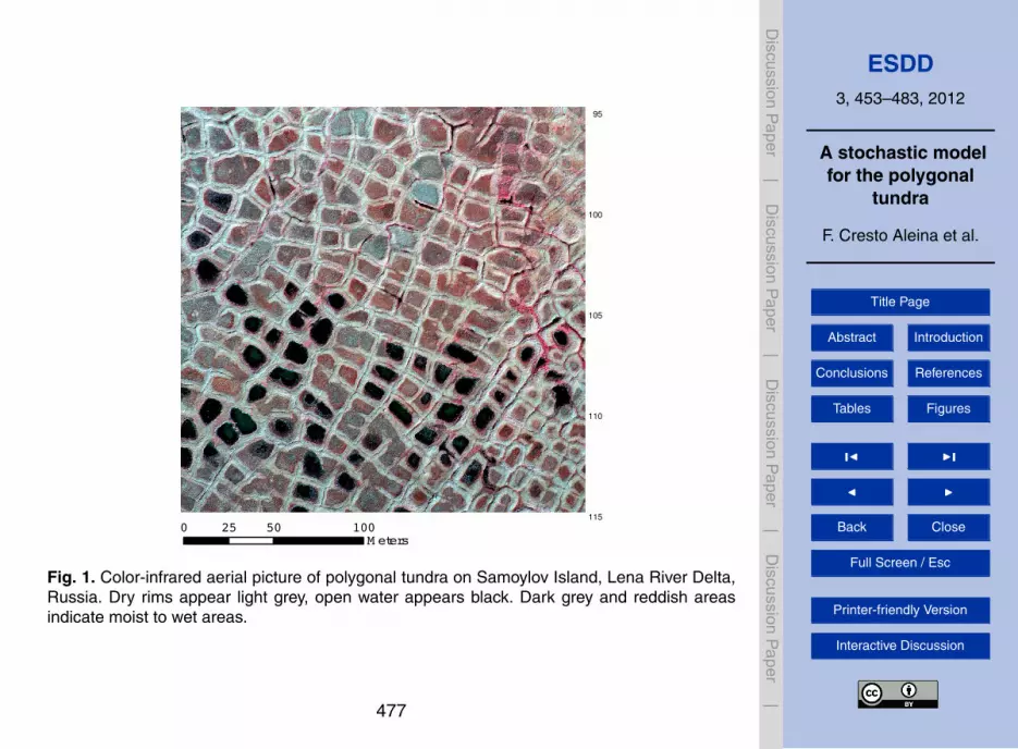
vegetation patterns in the polygonal landscapes. They have therefore been the focusof extensive field studies on experimental sites on Samoylov Island in the Lena RiverDelta in Siberia (an aerial picture of the study site is shown in Fig. 1). Previous worksinvolved closed-chamber and eddy covariance measurements of methane fluxes (seee.g. Sachs et al., 2008, 2010; Wille et al., 2008; Kutzbach et al., 2004), as well as mea-25

surements and modeling of hydrological properties (Boike et al., 2008), and of surfaceenergy balance (Langer et al., 2011b,a) in this typical periglacial landscape. Recentstudies with the help of remote sensing data were able to capture and analyze surfaceheterogeneity (land cover and surface temperature) and its importance for the land

456

ESDD3, 453–483, 2012

A stochastic modelfor the polygonal

tundra

F. Cresto Aleina et al.

Title Page

Abstract Introduction

Conclusions References

Tables Figures

J I

J I

Back Close

Full Screen / Esc

Printer-friendly Version

Interactive Discussion

Discussion

Paper

|D

iscussionP

aper|

Discussion

Paper

|D

iscussionP

aper|

atmosphere water fluxes (Muster et al., 2012; Langer et al., 2010). Theoretical effortshave also managed to quantitatively classify ice-wedge polygons and other permafrostpatterns in Alaska using Minkowski densities (Roth et al., 2005).

In general, stochastic models may be useful tools to link different scales. Such anapproach has been widely used in modeling physical, biological, and ecological phe-5

nomena, seeking to represent only the main processes and observable properties, andreplacing complex dynamics with random processes (see e.g. Dieckmann et al., 2000,and references therein). To model large-scale (e.g. 100 km2) seasonal dynamics of thesmall-scale-driven greenhouse gas emissions from such a landscape, it is impossibleto limit the description to an accurate model for a single polygon (typical dimensions10

in the order of 10 m in diameter), due to the wide internal variability of the landscape.In particular, this mechanistic approach would require a large number of parametersand computational power, in order to represent polygon variability in size, water tableposition with respect to the surface, and response to climatic forcing. In this work, weprovide a stochastic method that takes into account such variability, using properties of15

Voronoi polygons.Voronoi diagrams (or tessellations) have been applied to various field, from astron-

omy to biology, forestry, and crystallography. For comprehensive reviews, see e.g. Lu-carini (2009), Okabe et al. (2000), and reference therein. Their wide range of appli-cations derives from the fairly simple concept of partitioning the space behind them20

and from their adaptability. In ecology and Earth science, they have been used to de-scribe ecological subdivision of territories (Hasegawa and Tanemura, 1976), hydrologyand precipitation, geology, and recently also as framework in order to integrate climaticvariables over an irregular geographic region (Lucarini et al., 2008).

2 The model25

We develop a stochastic model, which is able to reproduce the main statistical charac-teristics of the low center polygonal tundra (i.e. surface topography, area of different soil

457

ESDD3, 453–483, 2012

A stochastic modelfor the polygonal

tundra

F. Cresto Aleina et al.

Title Page

Abstract Introduction

Conclusions References

Tables Figures

J I

J I

Back Close

Full Screen / Esc

Printer-friendly Version

Interactive Discussion

Discussion

Paper

|D

iscussionP

aper|

Discussion

Paper

|D

iscussionP

aper|

surfaces, water table height). With the present model we do not seek to explain surfacepattern formation: our aim is, instead, to find a robust way to upscale land-atmospheregreenhouse gas fluxes and the landscape response to climatic forcings that are cou-pled to these statistics. We limit our description to the landscape present-day state,and we do not represent polygon formation nor degradation.5

We tessellate the plane with random polygons which are able to reproduce the maingeneral features of ice-wedge polygons. The model represents, analyzes and con-siders the statistical characteristics of a region covered by ice-wedge polygons anddescribes the landscape-scale (about 1 km2 or more) response to climatic forcing. Inorder to represent represent ice-wedge polygonal tundra we use a random tessellation10

of the plane, the so-called Poisson-Voronoi Diagrams (Okabe et al., 2000).

2.1 Poisson-Voronoi Diagrams

Let us populate a Euclidean plane with an at most countable number of distinct points.We then associate all regions in that space with the closest member(s) of the pointset with respect to the Euclidean distance. The result is a set of regions that cover15

the whole plane, and each one of them is associated with a member of the generatingpoints. This tessellation is called planar ordinary Voronoi diagram, generated by thepoint set. The regions constituting the Voronoi diagram are the Voronoi polygons. Morerigorously, let P = {x1, ..., xn} be the generating point set, where 2≤n≤∞ and xi 6=xjfor i 6= j , with i and j integers. The (ordinary) Voronoi polygon associated with xi is20

defined as:

V (xi ) ={x| ||x − xi || ≤ ||x − xj ||, i 6= j

}(1)

and the set given by

V = {V (x1) , ..., V (xn)} (2)

is the Voronoi tessellation. In our case, the generating process P is a homogeneous25

Poisson point process P (λ), where λ is the intensity of the process. Therefore, we458

ESDD3, 453–483, 2012

A stochastic modelfor the polygonal

tundra

F. Cresto Aleina et al.

Title Page

Abstract Introduction

Conclusions References

Tables Figures

J I

J I

Back Close

Full Screen / Esc

Printer-friendly Version

Interactive Discussion

Discussion

Paper

|D

iscussionP

aper|

Discussion

Paper

|D

iscussionP

aper|

call the resulting tessellation Poisson-Voronoi Diagram (PVD). Parameter λ basicallycontrols the density of the Poisson process. On a square L×L, the intensity of theprocess defined as:

λ =E [n]

L2(3)

where E [n] is the mean of the number n of generated points, which follows a Poisson5

distribution. Parameter λ directly regulates the polygon sizes. We tuned this quantitywith data from image analysis of the landscape (Muster et al., 2012). From Eq. (3),L=1 km and λ=7500. Since λL2 �1 we are in the thermodynamic limit and theboundary effects can be neglected. A model realization of PVD is shown in Fig. 2.

The area of polygons in a Poisson-Voronoi Diagram has been widely analyzed by10

numerous studies (Okabe et al., 2000). Direct numerical investigations showed that3-parameter generalized gamma distributions fit quite well the statistical properties ofthe PVD (Miles and Maillardet, 1982):

fA(x) =r b

qr xq−1e−bxr

Γ(qr

) , r > 0, b > 0, q > 0. (4)

Other distributions have also been used in the literature to describe the PVD area dis-15

tribution such as lognormal and 2-parameters gamma (from Eq. 4, one obtains the2-paramters gamma distribution if r =1), as reported by Okabe et al. (2000) and refer-ence therein.

2.2 Idealized polygons

Ice-wedge polygons are composed of two main regions: elevated drier rims and lower20

wet centers. In our model:

Apol = qApol + (1 − q)Apol = R + C (5)459

ESDD3, 453–483, 2012

A stochastic modelfor the polygonal

tundra

F. Cresto Aleina et al.

Title Page

Abstract Introduction

Conclusions References

Tables Figures

J I

J I

Back Close

Full Screen / Esc

Printer-friendly Version

Interactive Discussion

Discussion

Paper

|D

iscussionP

aper|

Discussion

Paper

|D

iscussionP

aper|

where Apol is the total polygon area, and R and C represent the area covered by ele-vated rims and the one covered by low centers respectively. Parameter q is a randomquantity varying between 0.35 and 0.7, which we tune according to observation data(Muster et al., 2012).

Each Voronoi-region represents a ice-wedge polygon and its vertical structure con-5

sists of a column, which parameterizes the water table level Wt, the thaw depth TD,and the low polygon center surface level S. Water table is a dynamical variable andresponds to climatic forcing, whereas thaw depth follows a prescribed behavior duringthe seasonal cycle. Surface level, polygon depth, thaw depth and water table level areinitialized randomly: we tune their mean values with data from available field observa-10

tions. All quantities are computed from the top elevation of rims, as shown in Fig. 3.If water table rises above the center surface, area C increases as well, following the

equation:

C′ = π

(√Cπ

+δW

tan α

)2

(6)

where C′ is the polygon center area after the water table rise δW and α is the angle15

between elevated rims and polygon center surface, parameterized as:

α =π4

log(10q)

which takes into account that the larger the rims, the steeper polygon walls become,as suggested by observations. Factor π

4 is needed not to exceed the limit αlim = π2 .

Computing water table (Wt) variations with respect to the polygon surface (S) is es-20

sential to estimate methane emissions (Sachs et al., 2008; Wille et al., 2008; Kutzbachet al., 2004). We distinguish between three kinds of surface types, depending on theposition of the water table with respect to the polygon center surface. If:

460

ESDD3, 453–483, 2012

A stochastic modelfor the polygonal

tundra

F. Cresto Aleina et al.

Title Page

Abstract Introduction

Conclusions References

Tables Figures

J I

J I

Back Close

Full Screen / Esc

Printer-friendly Version

Interactive Discussion

Discussion

Paper

|D

iscussionP

aper|

Discussion

Paper

|D

iscussionP

aper|

S − Wt > ε ⇒ Wet centers

|S − Wt| ≤ ε ⇒ Saturated centers

S − Wt < −ε ⇒ Moist centers

where threshold ε=10 cm has been inferred from observations of small-scale methane5

emissions (Sachs et al., 2010). They are controlled by the site’s water table height, anddifferent surface types correspond to different emitting characteristics. In particular,methane emissions from saturated centers are an order of magnitude larger than inthe case of moist centers or than emissions from dry rims.

2.3 Water table dynamics10

We simulate water table variations at each time step (i.e. each day). The time periodwe are looking at is the summer season, when the snow has already melted, and thawdepth deepens. The prognostic equation for water table dynamics is:

dWt

dt= P − ET − R − ∆St (7)

where water table height Wt responds dynamically to precipitation P , evapotranspiration15

ET, and lateral runoff R. Term ∆St represents the amount of water stored in the unsat-urated terrain that does not contribute to water table variations. Since we only focus onthe effect of surface heterogeneity on GHG emissions, P and ET are parameterized asuniform over the whole area, i.e. we do not apply any downscaling of climatic forcing.In particular, the two variables follow a simple random parameterization. In this way,20

we are able to simulate both dry and wet summers. We generate a random number ofrainy days (between 5 and 40). If the day t is a rainy day (r.d.), then:

P =

{Rp sin

( t+T6T π

)if 30 < t < 90

10 mmday sin

( t+T6T π

)else

(8)

461

ESDD3, 453–483, 2012

A stochastic modelfor the polygonal

tundra

F. Cresto Aleina et al.

Title Page

Abstract Introduction

Conclusions References

Tables Figures

J I

J I

Back Close

Full Screen / Esc

Printer-friendly Version

Interactive Discussion

Discussion

Paper

|D

iscussionP

aper|

Discussion

Paper

|D

iscussionP

aper|

where Rp is a randomly generated number, which tunes the amplitude of precipitationevents in the part of the summer season when main precipitation events are supposedto occur, and it is computed in mm/day. In particular, changing Rp changes drasticallythe amount of incoming water. T =30 days is hereinafter a time constant. Similarly,evapotranspiration during one specific r.d. is parameterized as:5

ET = ETp sin(t + T6T π

)(9)

where ETp follows:

ETp =

5 mm

day if t = r.d. ∧ 30 < t < 90

2.5 mmday if t = r.d. ∧ (t < 30 ∨ t > 90)

2 mmday else

. (10)

We also consider that, due to soil porosity and water holding capacity, water table risesdifferently inside and above the soil. The soil within the polygon centers is assumed10

to be peat, or at any rate loose organic matter-rich soil material: i.e. the water levelrises twice as much if S −Wt <−ε. Thaw depth, on the other hand, follows a seasonaltrend: its level depends on the time of the year the model is run at. With progress of thesummer, the depth of the seasonally thawed layer (frost table depth) increases reachingits maximum at the beginning of September. We keep thaw depth dynamics prescribed,15

i.e. we do not consider how temperature variations may affect the environment. Fromavailable observations, we assume thaw depth to behave as follows:

462

ESDD3, 453–483, 2012

A stochastic modelfor the polygonal

tundra

F. Cresto Aleina et al.

Title Page

Abstract Introduction

Conclusions References

Tables Figures

J I

J I

Back Close

Full Screen / Esc

Printer-friendly Version

Interactive Discussion

Discussion

Paper

|D

iscussionP

aper|

Discussion

Paper

|D

iscussionP

aper|

TD =

15 t

T cm if t < 30(15 + 20 ·

√t−TT

)cm if 30 < t < 90

const else

. (11)

During spring/early summer the ground is still frozen and water is kept inside the poly-gons. With progression of thaw depth during summer, neighboring polygons can be-come hydraulically connected. Field experiments show that water which was retainedinside a polygon by the frozen elevated rims may in this situation slowly flow through5

the active layer of the rims themselves, from one polygon to another or from polygoncenter to the ice-wedge channel network (Boike et al., 2008). This phenomenon is im-portant for the water balance: in this case we assume a constant drop of the watertable because of lateral runoff R:

R =

{2 if Wt < TD

0 else(12)10

where R is computed in mm day−1. Physically it represents both later surface and sub-surface runoff. After large precipitation events, not all the precipitation leads to changesin water table level, but part of it fills the unsaturated terrain of the unsaturated elevatedrims and unsaturated zones of the polygon center (storage: ∆St). This water balanceterm has been observed in field campaigns and it is supposed to have a stronger in-15

fluence at the beginning of our simulation time slice (July), when the upper layer ofthe soil is unsaturated, whereas storage capacity decreases with time until the wholeterrain is saturated. In our model we parameterize storage as an exponential function:

∆St =

{(P − ET)e− t

τ if P ≥ 15mmday−1

0 else(13)

463

ESDD3, 453–483, 2012

A stochastic modelfor the polygonal

tundra

F. Cresto Aleina et al.

Title Page

Abstract Introduction

Conclusions References

Tables Figures

J I

J I

Back Close

Full Screen / Esc

Printer-friendly Version

Interactive Discussion

Discussion

Paper

|D

iscussionP

aper|

Discussion

Paper

|D

iscussionP

aper|

where t is time and τ =45 days is the characteristic time at which ∆S is reduced to(P −ET)/e.

We integrate the model for 90 days, which is approximately the duration of the thawseason in northern Siberia (July–September). Our model does not include cold months,when the surface is covered by snow. We also do not consider early summer, when5

there is still little thaw depth. External climatic forcings are precipitation and evapo-transpiration. We can vary precipitation intensity and its seasonal amount by tuningparameter Rp (Eq. 8). In our simulation, we use: Rp =30 mm day−1 for a standard sce-

nario, Rp =10 mm day−1 for a dry scenario and Rp =60 mm day−1 for a wet scenario.For each scenario, we perform ensemble simulations, calculate the average of 30 en-10

semble members, and compute water table dynamics. We finally derive variations onthe amount of landscape area covered by different surface characteristics (i.e. moistcenters, saturated centers or wet centers).

In order to give an example of the influence of of water table and surface wetnesson methane fluxes accounting for different climatic forcing, we multiply the area cov-15

ered by moist, saturated, or wet centers by values which represent the average Augustmethane emissions from each surface type (Sachs et al., 2010). Average methane flux(in mg per day) from the total region at each daily time step is computed following theequation:

Ftot = σCsaturated + ωCwet + δ (Cmoist + R) (14)20

where σ =94.1 mg d−1 m−2, ω=44.9 mg d−1 m−2, and δ =7.7 mg d−1 m−2. Values aretaken from Table 4 of Sachs et al. (2010). Area Ci of polygon centers with differentwetness and area R of relatively dry rims are computed in m2. In this simple model, weassume polygon rims and moist centers to have the same emission coefficient δ.

464

ESDD3, 453–483, 2012

A stochastic modelfor the polygonal

tundra

F. Cresto Aleina et al.

Title Page

Abstract Introduction

Conclusions References

Tables Figures

J I

J I

Back Close

Full Screen / Esc

Printer-friendly Version

Interactive Discussion

Discussion

Paper

|D

iscussionP

aper|

Discussion

Paper

|D

iscussionP

aper|

2.4 PVD and percolation theory

Mathematical properties of PVD are also well suited to describe some landscape-scalephysical processes that have been observed in the field. In particular, we focus oninterconnectivity properties of the graph, applying percolation theory on PVD.

When water flows from polygon centers trough the unfrozen top layers of the rims5

(lateral runoff), it starts to flow into channels on top of the ice wedges between thepolygon rims (visible in Fig. 1). Due to thermal erosion, water does not stay confinedin the channel, but flows through a path of interconnected channels. If this path ofchannels is large enough to connect polygons from one side of the landscape unitof consideration to the other one, we can assume that water in the channel is able10

to flow from one side to the other one. The system tested in this study is an island.Consequently, water which was previously confined in the channels would likely runoff the island to the near Lena river. In our model we assume interpolygonal channels(polygon edges in the PVD, or bonds, in percolation theory) to be active if the polygonexperiences lateral subsurface runoff. We also assume the polygon channel system to15

be flat, or with a very small topological gradient, so that no outflow due to landscapeslope is negligible.

Percolation theory describes the behavior of connected clusters in a random graph:since its introduction in the late fifties (Broadbent and Hammersley, 1957), it has beenwidely and successfully applied to a large number of fields, from network theory to20

biological evolution, and from galactic formation to forest fires (Grimmett, 1999, andreferences therein). Originally, the question to be answered focused on transport inporous media. Let us imagine a porous stone touching some water on a side: whatis the probability that the water passes through the whole stone, coming out at theother side? This simple question led to a basic stochastic model for such a situation25

and gave birth to percolation theory. In our model, the question would be: what is theprobability that an open path of interconnected channels is formed? This is in fact theprobability that a giant cluster of channels with flowing water appears. On the PVD,

465

ESDD3, 453–483, 2012

A stochastic modelfor the polygonal

tundra

F. Cresto Aleina et al.

Title Page

Abstract Introduction

Conclusions References

Tables Figures

J I

J I

Back Close

Full Screen / Esc

Printer-friendly Version

Interactive Discussion

Discussion

Paper

|D

iscussionP

aper|

Discussion

Paper

|D

iscussionP

aper|

bonds connecting two points of the graph represent channels. Water flowing throughrims enters the channel network generated above the ice wedges between the poly-gons. These channels are underlain by ice-wedges, and water flowing through themmay also cause thermo-erosion because of its mechanical and thermal effects on flow-ing water on ice. In our simple model, if a channel is filled by water, we call it active.5

Since we assume the environment not to have any slope, all edges of a polygon withWt <TD become active at the same time.

Percolation theory focuses on the probability θ(p) that a giant cluster exists. Thisprobability is non zero only if the probability p that a bond is active exceeds the criticalthreshold values pc. This value depends on the graph. Recent studies (Becker and Ziff,10

2009) determined numerically the bond percolation threshold pc on a PVD:

pc = 0.666931 ± 0.000005.

In order to reach percolation, the condition Wt <TD must be reached in a large enoughnumber of polygons. We simulate this result by keeping the thaw depth constant andincreasing the water table. We do not consider any physical process involved in water15

table change, but we keep increasing its level until we reach the percolation threshold.

3 Results and discussion

In this section we analyze environment statistics by comparing model outputs withavailable observations, both from field and from aerial photography. We analyze the ge-ometric characteristics of the polygonal tundra and the ones of PVD. We then present20

and discuss results from 90 days of simulations, and the water table dynamics in differ-ent simulated scenarios. Finally, we show results from our bond percolation realization.Our results are qualitatively different from a mean field approximation approach, sincemean water table variations are computed considering processes taking place in eachsingle polygon.25

466

ESDD3, 453–483, 2012

A stochastic modelfor the polygonal

tundra

F. Cresto Aleina et al.

Title Page

Abstract Introduction

Conclusions References

Tables Figures

J I

J I

Back Close

Full Screen / Esc

Printer-friendly Version

Interactive Discussion

Discussion

Paper

|D

iscussionP

aper|

Discussion

Paper

|D

iscussionP

aper|

3.1 Polygon statistics

We are interested in the distribution of areas covered by polygon centersC= (1−q)Apol. As for the polygon area Apol, we compare the histogram of model out-put for C with a generalized gamma distribution fA and a 2-parameters gamma distri-bution. Both distributions are accepted by a Kolmogorov-Smirnov test at a 0.05 level5

of confidence. Parameters of the distribution are taken from literature concerning thepolygon area distribution in a PVD (Okabe et al., 2000, and reference therein). Log-normal, exponential, and normal distributions are rejected by the test for both Apol andC.

We then proceed to compare the model results with available data for the ice-wedge10

polygons (Muster et al., 2012). We tuned the controlling parameter of the point processλ and the random parameter q (Eq. 5) with observed mean values of polygon andpolygon center areas. Results show that comparisons between model outputs anddata are quite robust: not only the first two statistical momenta are comparable, butthey also display a very similar distribution (as confirmed by a χ2 test at a 0.05 level of15

confidence).This result is central in our approach: it shows that PVD description of the landscape

statistics is consistent with observations. In particular, we claim that our approach isable to consistently capture the topographic features of the landscape we analyze.Even though the PVD are generated by a completely stochastic process (Poisson point20

process), they represent area distribution of such a complex environment as the thelow-center ice-wedge polygonal tundra. In order to test the robustness of this result,we performed simulations on an other less random tessellation, i.e. a regular squarelattice, with polygon area Apol equal to the mean area from observation data (136 m2).Again, polygon center area C= (1−q)Apol, with parameter q defined in the same way25

as for the random case. Even though mean polygon and polygon center areas havebeen tuned with observations, results do not fit polygon center distributions and fail

467

ESDD3, 453–483, 2012

A stochastic modelfor the polygonal

tundra

F. Cresto Aleina et al.

Title Page

Abstract Introduction

Conclusions References

Tables Figures

J I

J I

Back Close

Full Screen / Esc

Printer-friendly Version

Interactive Discussion

Discussion

Paper

|D

iscussionP

aper|

Discussion

Paper

|D

iscussionP

aper|

in particular to capture the skewness of the distribution, being therefore rejected byKolmogorov-Smirnov test.

3.2 Response to climatic forcing

Precipitation and evapotranspiration are the main inputs and outputs that drive waterlevel dynamics asdescribed in Eq. (7). In order to test the model response to drier and5

wetter conditions, we simulate different configurations by changing the amount of in-coming precipitation. We then compare the cumulative precipitation simulated by themodel and the one measured in the field, in order to have realistic scenarios compara-ble with data from field campaigns (Boike et al., 2008; Sachs et al., 2008). Field studiesobserved in particular the influence of lateral runoff and storage: water table drops in10

the late summer season, since water table usually lies above thaw depth, and it leadsto lateral fluxes of water in the ice-wedge channel network. The model captures boththis process (Fig. 5), as well as the variation magnitude.

odel results show that a decrease in precipitation will lead to a drastic drop in thewater table level, due to lateral runoff (Fig. 5b). Precipitation income is the only input15

in Eq. (7). Scenarios of such dry seasons are likely to lead to drastically drier soilconditions in the polygonal tundra landscapeif there is not a parallel decrease in meansurface temperature, and consequently in thaw depth behavior. On the other hand,an increase in precipitation with respect to the reference value used in the standardscenario will not cause a flooding of the landscape. In the wet scenario we perform20

simulations with a mean seasonal increase in precipitation of 100 mm yr−1 with respectto the reference value. In agreement with observations, mean water table changes itsposition by lying slightly above the average polygon surface (i.e. Wt <ε=10 cm).

Depending on Wt position in respect to the surface of the polygon center, soil charac-teristics in polygon centers vary from moist to saturated and wet conditions. Field stud-25

ies showed a link between water table position and emissions of greenhouse gases,especially methane (Kutzbach et al., 2004; Sachs et al., 2010) and latent heat fluxes(Langer et al., 2011b; Muster et al., 2012). In particular, methane fluxes vary up to an

468

ESDD3, 453–483, 2012

A stochastic modelfor the polygonal

tundra

F. Cresto Aleina et al.

Title Page

Abstract Introduction

Conclusions References

Tables Figures

J I

J I

Back Close

Full Screen / Esc

Printer-friendly Version

Interactive Discussion

Discussion

Paper

|D

iscussionP

aper|

Discussion

Paper

|D

iscussionP

aper|

order of magnitude among different surface types. Therefore dynamics of water tablealso influences dynamics of GHG emissions. Therefore, the situation predicted by themodel in the wet scenario could cause a large increase in emissions of methane Onceagain, temperature variations and influences on thaw depth seasonal behavior are ne-glected. If mean surface temperature rises, we expect lateral runoff to start earlier in5

the season and therefore to be able to drain more water away from the environment. Inour wet scenario precipitation further increases. In this case, runoff is not sufficient tobalance the excess water, and the area covered by wet centers increases.

Our model is also able to calculate the seasonal dynamics of the landscape areacovered by moist centers, saturated centers, and wet centers. These results are depen-10

dent on thaw depth dynamics, which we here assume prescribed. Overall, ensembleaverages of simulations in the three different scenarios we used for precipitation in-put, the fraction of area covered by saturated centers shows little seasonal dynamics ifcompared to the fraction of surface covered by wet and moist centers. According to ourmodel, during the summer only extreme drops in water table, or on the other hand very15

wet summers would lead to significant modifications to the fraction of the landscapecovered by saturated centers. We argue though, that coupling our simple approachto available permafrost models, and thus with thaw depth behaviors dependent on cli-matic and environmental conditions, would enable more realistic predictions in differentscenarios. In particular, in warmer conditions, soil could thaw deeper and earlier in the20

season, leading to further drops in the water table level and in the fraction of the land-scape covered by different terrains. The simple model here introduced for computingmethane emissions is directly related to changes in different surface properties. Weshow the results of ensemble simulations in different scenarios in the second panel ofFig. 5b. In particular, we observe that a decrease in precipitation (dry scenario) leads25

to a parallel decrease of methane emissions with respect to the standard case, mainlybecause of spreading of relatively drier tundra, which presents lower methane fluxesthan wet and saturated centers. Water table decreases and more and more centersbecome drier. According to Eq. (6), the area of the lower center decreases at the same

469

ESDD3, 453–483, 2012

A stochastic modelfor the polygonal

tundra

F. Cresto Aleina et al.

Title Page

Abstract Introduction

Conclusions References

Tables Figures

J I

J I

Back Close

Full Screen / Esc

Printer-friendly Version

Interactive Discussion

Discussion

Paper

|D

iscussionP

aper|

Discussion

Paper

|D

iscussionP

aper|

time, thus increasing the area covered by rims R, which in our model have the sameemission properties of drier centers. If precipitation increases, our model predicts a cor-responding increase in methane emission from the landscape. In this extreme case, amore elevated water table would lead to an increased number of wet centers, causinga retreat of the relatively drier tundra. Even though area covered by high-emissive sat-5

urated centers decreases, in fact, the decrease of surface covered by relatively driercenters is even larger. This situation is likely to increase methane emissions in respectto the standard scenario. Our results are only qualitative, since we assume only a fixedaverage value for the seasonal methane emissions.

3.3 Percolation threshold10

Figure 7 shows a bond percolation realization. We reach the bond percolation thresh-old by increasing the water table with a constant thaw depth. More and more polygonsexperience lateral runoff. Consequently, their channels become active and water flowsinto the channel network. The number of active channels needed to reach bond per-colation is given by the theoretical findings described above, and it increases with a15

rising water table. We expected the system to reach the percolation threshold if theaverage water table level lies above the thaw depth, but the correlation between thesetwo phenomena is not trivial. In particular, the system does not reach the percolationthreshold at the same time as the average water level is above the average surface. Inthe real system, if an interpolygonal channel is active, i.e. filled with water, water would20

not stay confined in it, but would spread to other empty channels because of gravity.This means that as only single polygons show lateral runoff, this drainage water wouldbe distributed to a certain number of other topographically connected channels, thusthe overall increase of water level within the channels would be dampened. If manypolygons experience lateral runoff, the number of empty channels would be drastically25

reduced. The water of the active channels could then spread in fewer channels. There-fore, the average water level within the channel network would increase. In this case,if a physical threshold somehow analogous to the percolation threshold on the PVD

470

ESDD3, 453–483, 2012

A stochastic modelfor the polygonal

tundra

F. Cresto Aleina et al.

Title Page

Abstract Introduction

Conclusions References

Tables Figures

J I

J I

Back Close

Full Screen / Esc

Printer-friendly Version

Interactive Discussion

Discussion

Paper

|D

iscussionP

aper|

Discussion

Paper

|D

iscussionP

aper|

would reached, the water which was confined in the network channel is likely to flowout of the system, namely into a near river, or sea. This phenomenon may also havea significant impact on the carbon balance of the system since the outflow of waterfrom the channel is one of the most important phenomena for the exchange of DOC(dissolved organic carbon) and DIC (dissolved inorganic carbon). Improving those fea-5

tures could be a future development of our approach, and the focus of further studies,more specifically interested at landscape-scale processes of periglacial environment.Nevertheless, a simple application of mathematical properties of PVD is able to cap-ture landscape-scale behavior of the system. In particular, the number of polygonsneeded to reach outflow can be easily computed through a bond percolation model. At10

this stage, water can flow from the system into a near river, or to the sea and wouldbe lost. Consequences of strong runoff events are ignored in our model but field ob-servations suggest that thermoerosion and water runoff could be agents for polygondegradation. We argue that the ability of PVD to simulate a physical process throughcritical thresholds enhances the power and the theoretical predictive capability of our15

approach.

4 Summary and conclusions

Our model provides a simple, stochastic, and consistent approach to upscale the ef-fect of local heterogeneities on GHG emissions at the landscape scale. In particular,we show how applications of Poisson-Voronoi Diagrams can statistically represent the20

main geometric and physic properties of the low-center ice-wedge polygonal tundra.We describe the landscape using Poisson Voronoi diagrams, tuning model charac-

teristics with field data. We show that the probability density function of modeled poly-gon center areas is consistent with the one inferred by observations. Our approach istherefore able to statistically upscale the terrain geometrical characteristics.25

Dynamical water table variations in respect to the polygon surface are essential tocompute methane fluxes, and we compute such variations during the summer season

471

ESDD3, 453–483, 2012

A stochastic modelfor the polygonal

tundra

F. Cresto Aleina et al.

Title Page

Abstract Introduction

Conclusions References

Tables Figures

J I

J I

Back Close

Full Screen / Esc

Printer-friendly Version

Interactive Discussion

Discussion

Paper

|D

iscussionP

aper|

Discussion

Paper

|D

iscussionP

aper|

over the whole region, parameterizing processes within the single polygons. Resultsof water table dynamics agree with observations. In particular, the stochastic modelis able to represent the water balance over the whole landscape. The model relatesthen the water table position to different soil wetness levels. In particular, we are ableto compute for each time step the fraction of the landscape covered by moist tundra5

(moist centers and polygon rims), saturated centers, and wet centers, under differentclimatic forcing.

Our modeling framework enables us to investigate effects of large scale interconnec-tivity among ice-wedge channel network. Applications of percolation thresholds on thePVD suggest possible explanations for water runoff from the landscape.10

The stochastic parameterization of our model is far from the precision and accu-racy of a mechanistic model. Mechanistic models, however, can reach accuracy onlyat the local scale whereas our approach accounts for landscape-scale properties andprocesses. Our presented approach could be further improved by including parameter-ization of hydrology, characterization of ice wedges and phenomena like thermokarst15

and polygon degradation. In particular, we argue that linking this approach with avail-able permafrost models would enable even more realistic predictions of water tableposition and the seasonal development of different surface types. Both variables arefundamental to consistently predict GHG emissions from polygonal tundra.

This model shows a new approach that could be successfully applied to other envi-20

ronments and ecosystems where local processes play an important role and a meanfield approximation would fail in estimating large scale features. Overall, the generalagreement between field measurements and model results suggests that statisticalmethods and simple parameterizations, if accurately tuned with field data, could be apowerful way to consider spatial scale interactions in such heterogenous and complex25

environments.

Acknowledgements. The authors are grateful to Moritz Langer for comments and discussionsthat significantly improved this article.

472

ESDD3, 453–483, 2012

A stochastic modelfor the polygonal

tundra

F. Cresto Aleina et al.

Title Page

Abstract Introduction

Conclusions References

Tables Figures

J I

J I

Back Close

Full Screen / Esc

Printer-friendly Version

Interactive Discussion

Discussion

Paper

|D

iscussionP

aper|

Discussion

Paper

|D

iscussionP

aper|

References

Baird, A. J., Belyea, L. R., and Morris, P. J.: Carbon Cycling in Northern Peatlands, volume 184of Geophysical Monograph Series, ISBN 978-0-87590-449-8, American Geophysical Union,Washington, D. C., doi:10.1029/GM184, 2009. 455

Becker, A. and Ziff, R.: Percolation thresholds on two-dimensional Voronoi networks and De-5

launay triangulations, Phys. Rev. E, 80, 1–9, doi:10.1103/PhysRevE.80.041101, 2009. 466Boike, J., Wille, C., and Abnizova, A.: Climatology and summer energy and water bal-

ance of polygonal tundra in the Lena River Delta, Siberia, J. Geophys. Res., 113, 1–15,doi:10.1029/2007JG000540, 2008. 456, 463, 468

Broadbent, S. and Hammersley, J.: Percolation processes, in: Mathematical Proceedings of the10

Cambridge Philosophical Society, volume 53, Cambridge Univ. Press, 629–641, 1957. 465Christensen, T. and Cox, P.: Response of methane emission from Arctic tundra to cli-

matic change: results from a model simulation, Tellus B, 47, 301–309, doi:10.1034/j.1600-0889.47.issue3.2.x, 1995. 455

Christensen, T., Lloyd, D., Svensson, B., Martikainen, P., Harding, R., Oskarsson, H., Soe-15

gaards, H., Friborg, T., and Panikov, N.: Biogenic controls on trace gas fluxes in northernwetlands, Global Change Newslett., 51, 9–15, 2001. 455

Dekker, S. C., Rietkerk, M., and Bierkens, M. F.: Coupling microscale vegetation – soil waterand macroscale vegetation – precipitation feedbacks in semiarid ecosystems, Global ChangeBiol., 1–8, doi:10.1111/j.1365-2486.2006.01327.x, 2007. 45420

Dieckmann, U., Law, R., and Metz, J. A. J.: The Geometry of Ecological Interactions,ISBN 0521642949, Cambridge University Press, doi:10.1017/CBO9780511525537, 2000.457

French, H.: The periglacial environment, 3rd Edn., ISBN 047086589X, Wiley, West Sussex,England, 2007. 45625

Grimmett, G.: Percolation, 2nd Edn., ISBN 3540649026, Springer-Verlag, New York, 1999. 465Haltigin, T., Pollard, W., and Dutilleul, P.: Statistical evidence of polygonal terrain self organi-

zation on earth and mars, in: Lunar and Planetary Institute Science Conference Abstracts,volume 42, 42nd Lunar and Planetary Science Conference, 7–11 March 2011, LPI Contribu-tion, The Woodlands, Texas, p. 1622, 2011. 45630

Hasegawa, M. and Tanemura, M.: On the pattern of space division by territories, Ann. Inst. Stat.Math., 28, 509–519, 1976. 457

473

ESDD3, 453–483, 2012

A stochastic modelfor the polygonal

tundra

F. Cresto Aleina et al.

Title Page

Abstract Introduction

Conclusions References

Tables Figures

J I

J I

Back Close

Full Screen / Esc

Printer-friendly Version

Interactive Discussion

Discussion

Paper

|D

iscussionP

aper|

Discussion

Paper

|D

iscussionP

aper|

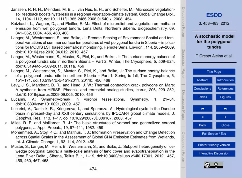
Janssen, R. H. H., Meinders, M. B. J., van Nes, E. H., and Scheffer, M.: Microscale vegetation-soil feedback boosts hysteresis in a regional vegetation-climate system, Global Change Biol.,14, 1104–1112, doi:10.1111/j.1365-2486.2008.01540.x, 2008. 454

Kutzbach, L., Wagner, D., and Pfeiffer, E.-M.: Effect of microrelief and vegetation on methaneemission from wet polygonal tundra, Lena Delta, Northern Siberia, Biogeochemistry, 69,5

341–362, 2004. 456, 460, 468Langer, M., Westermann, S., and Boike, J.: Remote Sensing of Environment Spatial and tem-

poral variations of summer surface temperatures of wet polygonal tundra in Siberia – implica-tions for MODIS LST based permafrost monitoring, Remote Sens. Environ., 114, 2059–2069,doi:10.1016/j.rse.2010.04.012, 2010. 45710

Langer, M., Westermann, S., Muster, S., Piel, K., and Boike, J.: The surface energy balance ofa polygonal tundra site in northern Siberia – Part 2: Winter, The Cryosphere, 5, 509–524,doi:10.5194/tc-5-509-2011, 2011a. 456

Langer, M., Westermann, S., Muster, S., Piel, K., and Boike, J.: The surface energy balanceof a polygonal tundra site in northern Siberia – Part 1: Spring to fall, The Cryosphere, 5,15

151–171, doi:10.5194/tc-5-151-2011, 2011b. 456, 468Levy, J. S., Marchant, D. R., and Head, J. W.: Thermal contraction crack polygons on Mars:

A synthesis from HiRISE, Phoenix, and terrestrial analog studies, Icarus, 206, 229–252,doi:10.1016/j.icarus.2009.09.005, 2010. 456

Lucarini, V.: Symmetry-break in voronoi tessellations, Symmetry, 1, 21–54,20

doi:10.3390/sym1010021, 2009. 457Lucarini, V., Danihlik, R., Kriegerova, I., and Speranza, A.: Hydrological cycle in the Danube

basin in present-day and XXII century simulations by IPCCAR4 global climate models, J.Geophys. Res., 113, 1–17, doi:10.1029/2007JD009167, 2008. 457

Miles, R. E. and Maillardet, R. J.: The basic structures of voronoi and generalized voronoi25

polygons, J. Appl. Probab., 19, 97–111, 1982. 459Mohammed, A., Stoy, P. C., and Malthus, T. J.: Information Preservation and Change Detection

across Spatial Scales in the Assessment of Global CH4 Emission Estimates from Wetlands,Int. J. Climate Change, 1, 93–114, 2012. 456

Muster, S., Langer, M., Heim, B., Westermann, S., and Boike, J.: Subpixel heterogeneity of ice-30

wedge polygonal tundra: a multi-scale analysis of land cover and evapotranspiration in theLena River Delta , Siberia, Tellus B, 1, 1–19, doi:10.3402/tellusb.v64i0.17301, 2012. 457,459, 460, 467, 468

474

ESDD3, 453–483, 2012

A stochastic modelfor the polygonal

tundra

F. Cresto Aleina et al.

Title Page

Abstract Introduction

Conclusions References

Tables Figures

J I

J I

Back Close

Full Screen / Esc

Printer-friendly Version

Interactive Discussion

Discussion

Paper

|D

iscussionP

aper|

Discussion

Paper

|D

iscussionP

aper|

O’Connor, F. M., Boucher, O., Gedney, N., Jones, C. D., Folberth, G. A., Coppell, R., Friedling-stein, P., Collins, W. J., Chappellaz, J., Ridley, J., and Johnson, C. E.: Possible role of wet-lands, permafrost, and methane hydrates in the methane cycle under future climate change:A review, Rev. Geophys., 48, 1–33, doi:10.1029/2010RG000326, 2010. 455

Okabe, A., Boots, B., Sugihara, K., and Chiu, S. N.: Spatial tessellations: concepts and appli-5

cations of Voronoi diagrams, ISBN 0471986356, 2nd Edn., John Wiley & Sons, 2000. 457,458, 459, 467

Pielke Sr., R. A., Avissar, R., Raupach, M., Dolman, A. J., Zeng, X., and Denning, A. S.: Interac-tions between the atmosphere and terrestrial ecosystems: influence on weather and climate,Global Change Biol., 4, 461–475, doi:10.1046/j.1365-2486.1998.t01-1-00176.x, 1998. 45410

Rietkerk, M., Brovkin, V., van Bodegom, P. M., Claussen, M., Dekker, S. C., Dijkstra, H. A., Gory-achkin, S. V., Kabat, P., van Nes, E. H., Neutel, A.-M., Nicholson, S. E., Nobre, C., Petoukhov,V., Provenzale, A., Scheffer, M., and Seneviratne, S. I.: Local ecosystem feedbacks andcritical transitions in the climate, Ecol. Complexity, 1–6, doi:10.1016/j.ecocom.2011.03.001,2011. 45415

Roth, K., Boike, J., and Vogel, H.-J.: Quantifying permafrost patterns using Minkowski densities,Permafrost Periglac. Process., 16, 277–290, doi:10.1002/ppp.531, 2005. 457

Sachs, T., Wille, C., Boike, J., and Kutzbach, L.: Environmental controls on ecosystem-scaleCH4 emission from polygonal tundra in the Lena River Delta, Siberia, J. Geophys. Res., 113,1–12, doi:10.1029/2007JG000505, 2008. 456, 460, 46820

Sachs, T., Giebels, M., Boike, J., and Kutzbach, L.: Environmental controls on CH4 emissionfrom polygonal tundra on the microsite scale in the Lena river delta, Siberia, Global ChangeBiol., 16, 3096–3110, doi:10.1111/j.1365-2486.2010.02232.x, 2010. 456, 461, 464, 468

Scheffer, M., Holmgren, M., Brovkin, V., and Claussen, M.: Synergy between small- and large-scale feedbacks of vegetation on the water cycle, Global Change Biol., 11, 1003–1012,25

doi:10.1111/j.1365-2486.2005.00962.x, 2005. 454Schuur, E. A. G., Bockheim, J., Canadell, J. G., Euskirchen, E., Field, C. B., Goryachkin, S. V.,

Hagemann, S., Kuhry, P., Lafleur, P. M., Lee, H., Mazhitova, G., Nelson, F. E., Rinke, A.,Romanovsky, V. E., Shiklomanov, N., Tarnocai, C., Venevsky, S., Vogel, J. G., and Zimov, S.A.: Vulnerability of Permafrost Carbon to Climate Change: Implications for the Global Carbon30

Cycle, BioScience, 58, 701–714, doi:10.1641/B580807, 2008. 455

475

ESDD3, 453–483, 2012

A stochastic modelfor the polygonal

tundra

F. Cresto Aleina et al.

Title Page

Abstract Introduction

Conclusions References

Tables Figures

J I

J I

Back Close

Full Screen / Esc

Printer-friendly Version

Interactive Discussion

Discussion

Paper

|D

iscussionP

aper|

Discussion

Paper

|D

iscussionP

aper|

Stoy, P. C., Williams, M., Spadavecchia, L., Bell, R. A., Prieto-Blanco, A., Evans, J. G., and Wijk,M. T.: Using Information Theory to Determine Optimum Pixel Size and Shape for EcologicalStudies: Aggregating Land Surface Characteristics in Arctic Ecosystems, Ecosystems, 12,574–589, doi:10.1007/s10021-009-9243-7, 2009. 456

Walter, B., Heimann, M., Shannon, R., and White, J.: A process-based model to derive methane5

emissions from natural wetlands, Geophys. Res. Lett., 23, 3731–3734, 1996. 455Walter, K. M., Zimov, S. A., Chanton, J. P., Verbyla, D., and Chapin, F. S.: Methane bubbling

from Siberian thaw lakes as a positive feedback to climate warming, Nature, 443, 71–75,doi:10.1038/nature05040, 2006. 455

Walter, P. and Heimann, M.: A process-based, climate-sensitive model to derive methane emis-10

sions from natural wetlands: Application to five wetland sites, sensitivity to model parameters,and climate, Global Biogeochem. Cy., 14, 745–765, 2000. 455

Wille, C., Kutzbach, L., Sachs, T., Wagner, D., and Pfeiffer, E.-M.: Methane emission fromSiberian arctic polygonal tundra: eddy covariance measurements and modeling, GlobalChange Biol., 14, 1395–1408, doi:10.1111/j.1365-2486.2008.01586.x, 2008. 456, 46015

Zhang, Y., Sachs, T., Li, C., and Boike, J.: Upscaling methane fluxes from closed chambers toeddy covariance based on a permafrost biogeochemistry integrated model, Global ChangeBiol., 18, 1428–1440, doi:10.1111/j.1365-2486.2011.02587.x, 2012. 455

476

ESDD3, 453–483, 2012

A stochastic modelfor the polygonal

tundra

F. Cresto Aleina et al.

Title Page

Abstract Introduction

Conclusions References

Tables Figures

J I

J I

Back Close

Full Screen / Esc

Printer-friendly Version

Interactive Discussion

Discussion

Paper

|D

iscussionP

aper|

Discussion

Paper

|D

iscussionP

aper|

2 F. Cresto Aleina: A stochastic model for the polygonal tundra

0 50 10025M eters

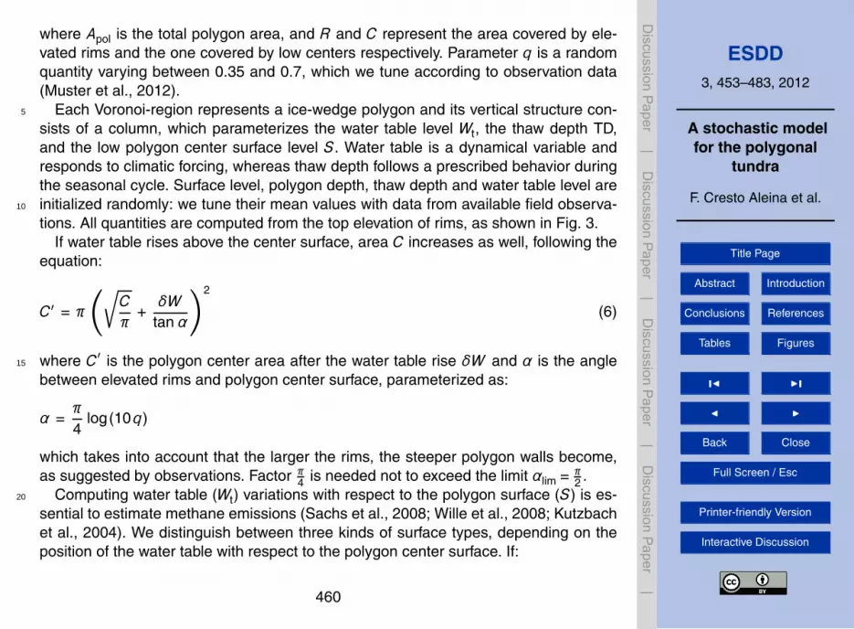
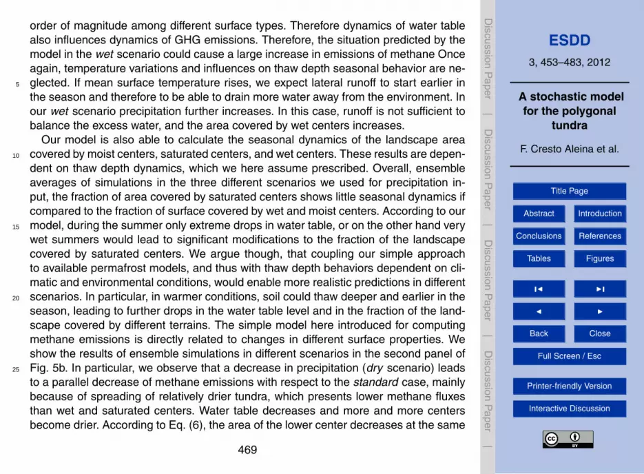
Fig. 1: Color-infrared aerial picture of polygonal tundra onSamoylov Island, Lena River Delta, Russia. Dry rims appearlight grey, open water appears black. Dark grey and reddishareas indicate moist to wet areas.

leads to a much better agreement with landscape scale emis-70

sions as measured by eddy covariance than previous upscal-ing attempts with process-based models that ignored the spa-tial heterogeneity.The model representation of such hetero-geneity is currently usually driven by the pixel size of avail-able remote sensing products or the grid cell size of the re-75

spective model, the real world functional or structural dif-ferences between individual components of a heterogeneousdomain may actually be on a very different scale. Preserv-ing their information content becomes particularly importantwhere nonlinear relationships are involved in the represented80

processes such as those driving greenhouse gas emissions(Stoy et al., 2009; Mohammed et al., 2012).

Arctic lowland landscapes underlain by permafrost aretypically characterized by patterned ground such as ice-wedge polygonal tundra. They cover approximately 5-10%85

of Earth’s land surface, where they play a dominant role indetermining surface morphology, drainage and patterns ofvegetation (French, 2007). Low center polygonal tundra typ-ically consists of elevated comparatively dry rims and lowercenters which can become wet if the water table rises to the90

ground surface level or above. Thermal induced cracking inthe soil during winters with large temperature drop generatesthe polygonal patterned ground. When the temperature risesand snow cover melts, water infiltrates in those cracks, and

refreezes. Over the years, as this process is cyclically iter-95

ated, the terrain is deformed due to the formation of verticalmasses of ice, called ice-wedges. Aside of the wedges, ter-rain is elevated because it is pushed upwards, forming theelevated rims typical of this landscape. Incoming water (pre-cipitation or snow melt) is then trapped by the rims in the100

polygon center, resulting in a water table level, which dy-namically responds to climate and weather. This environ-ment is typical for high-latitude permafrost areas of Alaska,Canada, and Siberia, and ice-wedge polygon features havebeen observed also on Mars (Haltigin et al., 2011; Levy et al.,105

2010). The surface morphology of dry rims and wet centersdetermines drainage and vegetation patterns in the polygonallandscapes. They have therefore been the focus of extensivefield studies on experimental sites on Samoylov Island in theLena River Delta in Siberia (an aerial picture of the study site110

is shown in Fig.1). Previous works involved closed-chamberand eddy covariance measurements of methane fluxes (seee.g. Sachs et al., 2008, 2010; Wille et al., 2008; Kutzbachet al., 2004), as well as measurements and modeling of hy-drological properties (Boike et al., 2008), and of surface115

energy balance (Langer et al., 2011, 2010b) in this typicalperiglacial landscape. Recent studies with the help of remotesensing data were able to capture and analyze surface het-erogeneity (land cover and surface temperature) and its im-portance for the land atmosphere water fluxes (Muster et al.,120

2012; Langer et al., 2010a). Theoretical efforts have alsomanaged to quantitatively classify ice-wedge polygons andother permafrost patterns in Alaska using Minkowski densi-ties (Roth et al., 2005).

In general, stochastic models may be useful tools to link125

different scales. Such an approach has been widely used inmodeling physical, biological, and ecological phenomena,seeking to represent only the main processes and observableproperties, and replacing complex dynamics with randomprocesses (see e.g. Dieckmann et al., 2000, and references130

therein). To model large-scale (e.g., 100 km2) seasonal dy-namics of the small-scale-driven greenhouse gas emissionsfrom such a landscape, it is impossible to limit the descrip-tion to an accurate model for a single polygon (typical di-mensions in the order of 10 m in diameter), due to the wide135

internal variability of the landscape. In particular, this mech-anistic approach would require a large number of parametersand computational power, in order to represent polygon vari-ability in size, water table position with respect to the surface,and response to climatic forcing. In this work, we provide a140

stochastic method that takes into account such variability, us-ing properties of Voronoi polygons.

Voronoi diagrams (or tessellations) have been applied tovarious field, from astronomy to biology, forestry, and crys-tallography. For comprehensive reviews, see e.g. Lucarini145

(2009), Okabe et al. (2000), and reference therein. Theirwide range of applications derives from the fairly simpleconcept of partitioning the space behind them and fromtheir adaptability. In ecology and Earth science, they have

Fig. 1. Color-infrared aerial picture of polygonal tundra on Samoylov Island, Lena River Delta,Russia. Dry rims appear light grey, open water appears black. Dark grey and reddish areasindicate moist to wet areas.

477

ESDD3, 453–483, 2012

A stochastic modelfor the polygonal

tundra

F. Cresto Aleina et al.

Title Page

Abstract Introduction

Conclusions References

Tables Figures

J I

J I

Back Close

Full Screen / Esc

Printer-friendly Version

Interactive Discussion

Discussion

Paper

|D

iscussionP

aper|

Discussion

Paper

|D

iscussionP

aper|

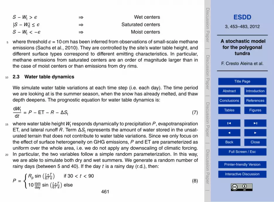
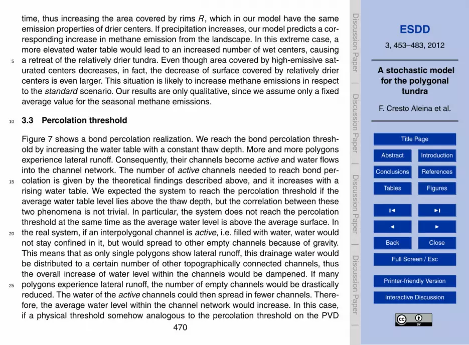
Fig. 2. Poisson-Voronoi Diagrams: different colors represent different types of surfaces: lightgreen if the polygon center is moist (water table>10 cm below the surface), dark green if it issaturated (water table<10 cm below as well as <10 cm above the surface) and blue if it is wet(water table>10 cm above the surface and the polygon is covered by open water). Dimensionsof polygon edges in the figure are not to scale, since in our model they cover up to 70 % of thewhole polygon area. Distances on x- and y-axes are in meters.

478

ESDD3, 453–483, 2012

A stochastic modelfor the polygonal

tundra

F. Cresto Aleina et al.

Title Page

Abstract Introduction

Conclusions References

Tables Figures

J I

J I

Back Close

Full Screen / Esc

Printer-friendly Version

Interactive Discussion

Discussion

Paper

|D

iscussionP

aper|

Discussion

Paper

|D

iscussionP

aper|

4 F. Cresto Aleina: A stochastic model for the polygonal tundra

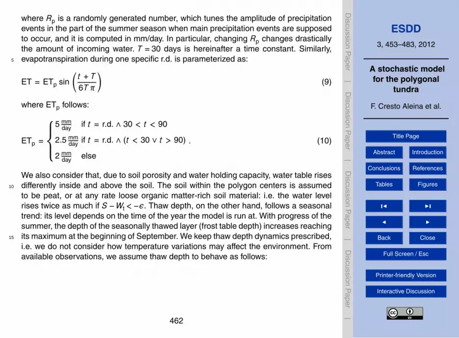
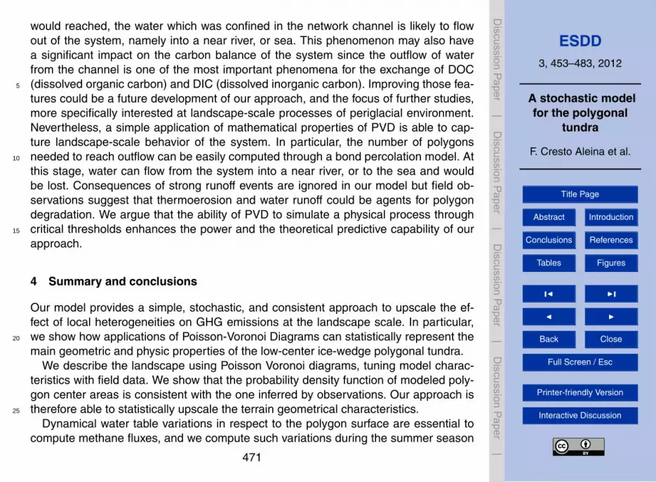
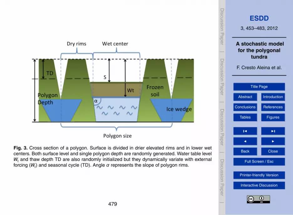
Fig. 3: Cross section of a polygon. Surface is divided in drierelevated rims and in lower wet centers. Both surface leveland single polygon depth are randomly generated. Water ta-ble level Wt and thaw depth TD are also randomly initial-ized but they dynamically variate with external forcing (Wt)and seasonal cycle (TD). Angle α represents the slope ofpolygon rims.

2.2 Idealized polygons

Ice-wedge polygons are composed of two main regions: ele-vated drier rims and lower wet centers. In our model:

Apol = qApol+(1−q)Apol =R+C (5)

where Apol is the total polygon area, and R and C represent190

the area covered by elevated rims and the one covered bylow centers respectively. Parameter q is a random quantityvarying between 0.35 and 0.7, which we tune according toobservation data (Muster et al., 2012).

Each Voronoi-region represents a ice-wedge polygon and195

its vertical structure consists of a column, which parameter-izes the water table level Wt, the thaw depth TD, and thelow polygon center surface level S. Water table is a dynam-ical variable and responds to climatic forcing, whereas thawdepth follows a prescribed behavior during the seasonal cy-200

cle. Surface level, polygon depth, thaw depth and water ta-ble level are initialized randomly: we tune their mean valueswith data from available field observations. All quantities arecomputed from the top elevation of rims, as shown in Fig. 3.

If water table rises above the center surface, area C in-creases as well, following the equation:

C ′=π

(√C

π+δW

tanα

)2

(6)

where C ′ is the polygon center area after the water table riseδW and α is the angle between elevated rims and polygon

center surface, parameterized as:

α=π

4log(10q)

which takes into account that the larger the rims, the steeper205

polygon walls become, as suggested by observations. Factorπ4 is needed not to exceed the limit αlim = π

2 .Computing water table (Wt) variations with respect to the

polygon surface (S) is essential to estimate methane emis-sions (Sachs et al., 2008; Wille et al., 2008; Kutzbach et al.,2004). We distinguish between three kinds of surface types,depending on the position of the water table with respect tothe polygon center surface. If:

S−Wt>ε ⇒ Wet centers|S−Wt| ≤ ε ⇒ Saturated centersS−Wt<−ε ⇒ Moist centers

where threshold ε= 10 cm has been inferred from observa-tions of small-scale methane emissions (Sachs et al., 2010).They are controlled by the site’s water table height, and dif-210

ferent surface types correspond to different emitting char-acteristics. In particular, methane emissions from saturatedcenters are an order of magnitude larger than in the case ofmoist centers or than emissions from dry rims.

2.3 Water table dynamics215

We simulate water table variations at each time step (i.e.,each day). The time period we are looking at is the summerseason, when the snow has already melted, and thaw depthdeepens. The prognostic equation for water table dynamicsis:

dWt

dt=P −ET −R−∆St (7)

where water table height Wt responds dynamically to pre-cipitation P , evapotranspiration ET , and lateral runoff R.Term ∆St represents the amount of water stored in the un-saturated terrain that does not contribute to water table vari-ations. Since we only focus on the effect of surface hetero-geneity on GHG emissions, P and ET are parameterized asuniform over the whole area, i.e. we do not apply any down-scaling of climatic forcing. In particular, the two variablesfollow a simple random parameterization. In this way, weare able to simulate both dry and wet summers. We generatea random number of rainy days (between 5 and 40). If theday t is a rainy day (r.d.), then:

P =

Rpsin( t+T6Tπ ) if 30<t< 90

10mmday sin( t+T6Tπ ) else

(8)

where Rp is a randomly generated number, which tunes theamplitude of precipitation events in the part of the summerseason when main precipitation events are supposed to occur,

Fig. 3. Cross section of a polygon. Surface is divided in drier elevated rims and in lower wetcenters. Both surface level and single polygon depth are randomly generated. Water table levelWt and thaw depth TD are also randomly initialized but they dynamically variate with externalforcing (Wt) and seasonal cycle (TD). Angle α represents the slope of polygon rims.

479

ESDD3, 453–483, 2012

A stochastic modelfor the polygonal

tundra

F. Cresto Aleina et al.

Title Page

Abstract Introduction

Conclusions References

Tables Figures

J I

J I

Back Close

Full Screen / Esc

Printer-friendly Version

Interactive Discussion

Discussion

Paper

|D

iscussionP

aper|

Discussion

Paper

|D

iscussionP

aper|

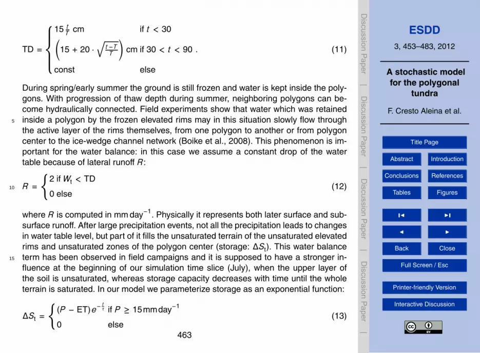
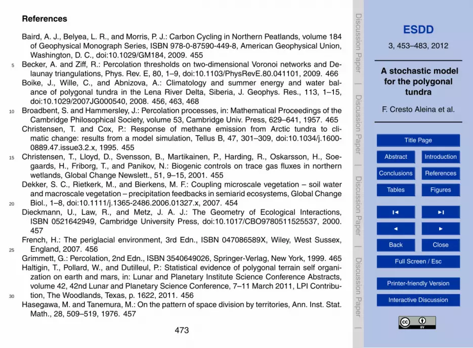
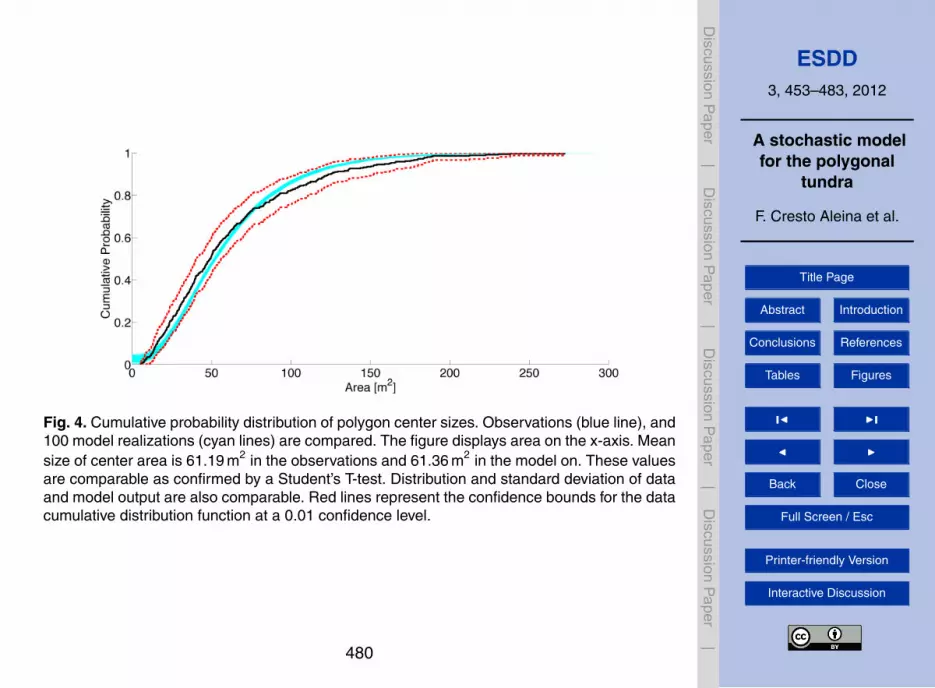
Fig. 4. Cumulative probability distribution of polygon center sizes. Observations (blue line), and100 model realizations (cyan lines) are compared. The figure displays area on the x-axis. Meansize of center area is 61.19 m2 in the observations and 61.36 m2 in the model on. These valuesare comparable as confirmed by a Student’s T-test. Distribution and standard deviation of dataand model output are also comparable. Red lines represent the confidence bounds for the datacumulative distribution function at a 0.01 confidence level.

480

ESDD3, 453–483, 2012

A stochastic modelfor the polygonal

tundra

F. Cresto Aleina et al.

Title Page

Abstract Introduction

Conclusions References

Tables Figures

J I

J I

Back Close

Full Screen / Esc

Printer-friendly Version

Interactive Discussion

Discussion

Paper

|D

iscussionP

aper|

Discussion

Paper

|D

iscussionP

aper|

F. Cresto Aleina: A stochastic model for the polygonal tundra 7

and the random parameter q (equation 5) with observed meanvalues of polygon and polygon center areas. Results showthat comparisons between model outputs and data are quiterobust: not only the first two statistical momenta are com-325

parable, but they also display a very similar distribution (asconfirmed by a χ2 test at a 0.05 level of confidence).

This result is central in our approach: it shows that PVDdescription of the landscape statistics is consistent with ob-servations. In particular, we claim that our approach is able330

to consistently capture the topographic features of the land-scape we analyze. Even though the PVD are generated by acompletely stochastic process (Poisson point process), theyrepresent area distribution of such a complex environmentas the the low-center ice-wedge polygonal tundra. In or-335

der to test the robustness of this result, we performed sim-ulations on an other less random tessellation, i.e. a regularsquare lattice, with polygon area Apol equal to the mean areafrom observation data (136 m2). Again, polygon center areaC = (1−q)Apol, with parameter q defined in the same way340

as for the random case. Even though mean polygon and poly-gon center areas have been tuned with observations, resultsdo not fit polygon center distributions and fail in particularto capture the skewness of the distribution, being thereforerejected by Kolmogorov-Smirnov test.345

3.2 Response to climatic forcing

Precipitation and evapotranspiration are the main inputs andoutputs that drive water level dynamics asdescribed in equa-tion 7. In order to test the model response to drier and wetterconditions, we simulate different configurations by chang-350

ing the amount of incoming precipitation. We then comparethe cumulative precipitation simulated by the model and theone measured in the field, in order to have realistic scenar-ios comparable with data from field campaigns (Boike et al.,2008; Sachs et al., 2008). Field studies observed in partic-355

ular the influence of lateral runoff and storage: water tabledrops in the late summer season, since water table usuallylies above thaw depth, and it leads to lateral fluxes of waterin the ice-wedge channel network. The model captures boththis process (Fig. 5), as well as the variation magnitude.360

Model results show that a decrease in precipitation willlead to a drastic drop in the water table level, due to lateralrunoff (Fig. 5b). Precipitation income is the only input inequation 7. Scenarios of such dry seasons are likely to leadto drastically drier soil conditions in the polygonal tundra365

landscapeif there is not a parallel decrease in mean surfacetemperature, and consequently in thaw depth behavior. Onthe other hand, an increase in precipitation with respect to thereference value used in the standard scenario will not causea flooding of the landscape. In the wet scenario we perform370

simulations with a mean seasonal increase in precipitation of100 mm/year with respect to the reference value. In agree-ment with observations, mean water table changes its posi-

(a)

(b)

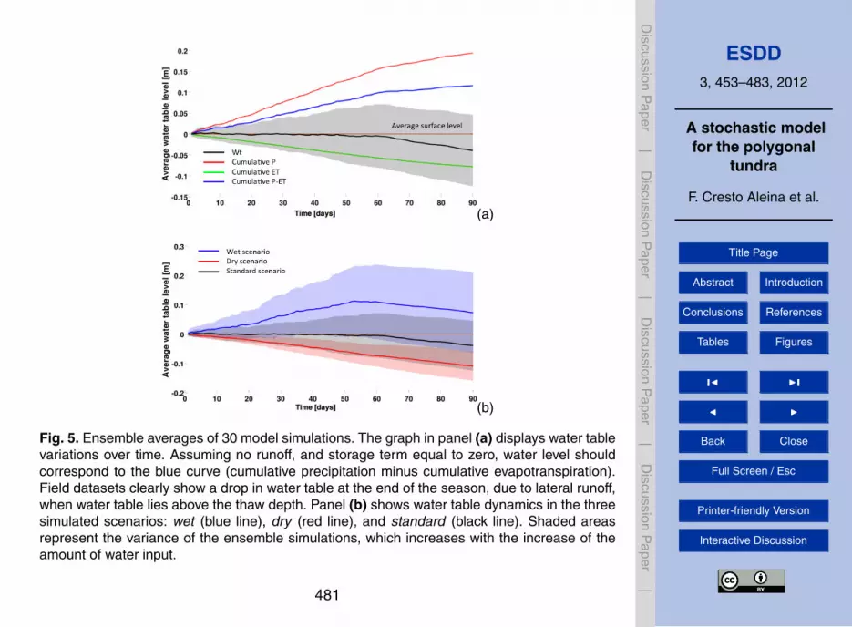
Fig. 5: Ensemble averages of 30 model simulations. Thegraph in panel (a) displays water table variations over time.Assuming no runoff, and storage term equal to zero, waterlevel should correspond to the blue curve (cumulative precip-itation minus cumulative evapotranspiration). Field datasetsclearly show a drop in water table at the end of the season,due to lateral runoff, when water table lies above the thawdepth. Panel (b) shows water table dynamics in the threesimulated scenarios: wet (blue line), dry (red line), and stan-dard (black line). Shaded areas represent the variance of theensemble simulations, which increases with the increase ofthe amount of water input.

tion by lying slightly above the average polygon surface (i.e,Wt<ε= 10 cm).375

Depending on Wt position in respect to the surface of thepolygon center, soil characteristics in polygon centers varyfrom moist to saturated and wet conditions. Field studiesshowed a link between water table position and emissionsof greenhouse gases, especially methane (Kutzbach et al.,380

2004; Sachs et al., 2010) and latent heat fluxes (Langer et al.,2011; Muster et al., 2012). In particular, methane fluxes varyup to an order of magnitude among different surface types.Therefore dynamics of water table also influences dynam-ics of GHG emissions. Therefore, the situation predicted by385

the model in the wet scenario could cause a large increase inemissions of methane Once again, temperature variations andinfluences on thaw depth seasonal behavior are neglected. Ifmean surface temperature rises, we expect lateral runoff to

(a)

F. Cresto Aleina: A stochastic model for the polygonal tundra 7

and the random parameter q (equation 5) with observed meanvalues of polygon and polygon center areas. Results showthat comparisons between model outputs and data are quiterobust: not only the first two statistical momenta are com-325

parable, but they also display a very similar distribution (asconfirmed by a χ2 test at a 0.05 level of confidence).

This result is central in our approach: it shows that PVDdescription of the landscape statistics is consistent with ob-servations. In particular, we claim that our approach is able330

to consistently capture the topographic features of the land-scape we analyze. Even though the PVD are generated by acompletely stochastic process (Poisson point process), theyrepresent area distribution of such a complex environmentas the the low-center ice-wedge polygonal tundra. In or-335

der to test the robustness of this result, we performed sim-ulations on an other less random tessellation, i.e. a regularsquare lattice, with polygon area Apol equal to the mean areafrom observation data (136 m2). Again, polygon center areaC = (1−q)Apol, with parameter q defined in the same way340

as for the random case. Even though mean polygon and poly-gon center areas have been tuned with observations, resultsdo not fit polygon center distributions and fail in particularto capture the skewness of the distribution, being thereforerejected by Kolmogorov-Smirnov test.345

3.2 Response to climatic forcing

Precipitation and evapotranspiration are the main inputs andoutputs that drive water level dynamics asdescribed in equa-tion 7. In order to test the model response to drier and wetterconditions, we simulate different configurations by chang-350

ing the amount of incoming precipitation. We then comparethe cumulative precipitation simulated by the model and theone measured in the field, in order to have realistic scenar-ios comparable with data from field campaigns (Boike et al.,2008; Sachs et al., 2008). Field studies observed in partic-355

ular the influence of lateral runoff and storage: water tabledrops in the late summer season, since water table usuallylies above thaw depth, and it leads to lateral fluxes of waterin the ice-wedge channel network. The model captures boththis process (Fig. 5), as well as the variation magnitude.360

Model results show that a decrease in precipitation willlead to a drastic drop in the water table level, due to lateralrunoff (Fig. 5b). Precipitation income is the only input inequation 7. Scenarios of such dry seasons are likely to leadto drastically drier soil conditions in the polygonal tundra365

landscapeif there is not a parallel decrease in mean surfacetemperature, and consequently in thaw depth behavior. Onthe other hand, an increase in precipitation with respect to thereference value used in the standard scenario will not causea flooding of the landscape. In the wet scenario we perform370

simulations with a mean seasonal increase in precipitation of100 mm/year with respect to the reference value. In agree-ment with observations, mean water table changes its posi-

(a)

(b)

Fig. 5: Ensemble averages of 30 model simulations. Thegraph in panel (a) displays water table variations over time.Assuming no runoff, and storage term equal to zero, waterlevel should correspond to the blue curve (cumulative precip-itation minus cumulative evapotranspiration). Field datasetsclearly show a drop in water table at the end of the season,due to lateral runoff, when water table lies above the thawdepth. Panel (b) shows water table dynamics in the threesimulated scenarios: wet (blue line), dry (red line), and stan-dard (black line). Shaded areas represent the variance of theensemble simulations, which increases with the increase ofthe amount of water input.

tion by lying slightly above the average polygon surface (i.e,Wt<ε= 10 cm).375

Depending on Wt position in respect to the surface of thepolygon center, soil characteristics in polygon centers varyfrom moist to saturated and wet conditions. Field studiesshowed a link between water table position and emissionsof greenhouse gases, especially methane (Kutzbach et al.,380

2004; Sachs et al., 2010) and latent heat fluxes (Langer et al.,2011; Muster et al., 2012). In particular, methane fluxes varyup to an order of magnitude among different surface types.Therefore dynamics of water table also influences dynam-ics of GHG emissions. Therefore, the situation predicted by385

the model in the wet scenario could cause a large increase inemissions of methane Once again, temperature variations andinfluences on thaw depth seasonal behavior are neglected. Ifmean surface temperature rises, we expect lateral runoff to

(b)

Fig. 5. Ensemble averages of 30 model simulations. The graph in panel (a) displays water tablevariations over time. Assuming no runoff, and storage term equal to zero, water level shouldcorrespond to the blue curve (cumulative precipitation minus cumulative evapotranspiration).Field datasets clearly show a drop in water table at the end of the season, due to lateral runoff,when water table lies above the thaw depth. Panel (b) shows water table dynamics in the threesimulated scenarios: wet (blue line), dry (red line), and standard (black line). Shaded areasrepresent the variance of the ensemble simulations, which increases with the increase of theamount of water input.

481

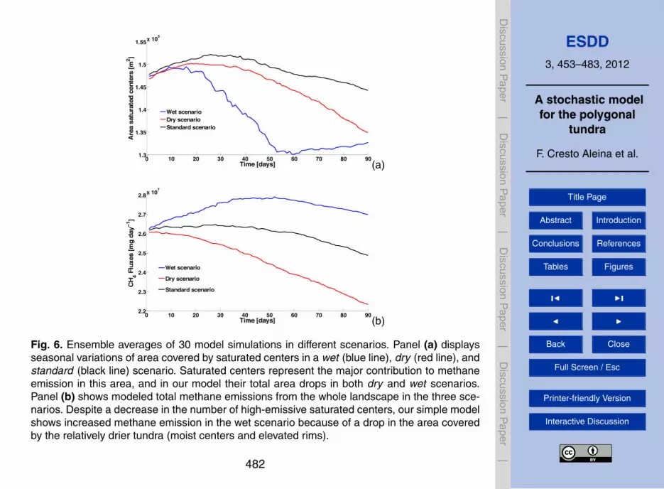
ESDD3, 453–483, 2012

A stochastic modelfor the polygonal

tundra

F. Cresto Aleina et al.

Title Page

Abstract Introduction

Conclusions References

Tables Figures

J I

J I

Back Close

Full Screen / Esc

Printer-friendly Version

Interactive Discussion

Discussion

Paper

|D

iscussionP

aper|

Discussion

Paper

|D

iscussionP

aper|

8 F. Cresto Aleina: A stochastic model for the polygonal tundra

0 10 20 30 40 50 60 70 80 901.3

1.35

1.4

1.45

1.5

1.55x 105

Time [days]

Area

sat

urat

ed c

ente

rs [m

2 ]

Wet scenarioDry scenarioStandard scenario

(a)

0 10 20 30 40 50 60 70 80 902.2

2.3

2.4

2.5

2.6

2.7

2.8x 107

Time [days]

CH

4 Flu

xes

[mg

day−

1 ]

Wet scenario

Dry scenario

Standard scenario

(b)

Fig. 6: Ensemble averages of 30 model simulations in dif-ferent scenarios. Panel (a) displays seasonal variations ofarea covered by saturated centers in a wet (blue line), dry(red line), and standard (black line) scenario. Saturated cen-ters represent the major contribution to methane emission inthis area, and in our model their total area drops in both dryand wet scenarios. Panel (b) shows modeled total methaneemissions from the whole landscape in the three scenarios.Despite a decrease in the number of high-emissive saturatedcenters, our simple model shows increased methane emissionin the wet scenario because of a drop in the area covered bythe relatively drier tundra (moist centers and elevated rims).

start earlier in the season and therefore to be able to drain390

more water away from the environment. In our wet scenarioprecipitation further increases. In this case, runoff is not suf-ficient to balance the excess water, and the area covered bywet centers increases.

Our model is also able to calculate the seasonal dynam-395

ics of the landscape area covered by moist centers, saturatedcenters, and wet centers. These results are dependent on thawdepth dynamics, which we here assume prescribed. Overall,ensemble averages of simulations in the three different sce-narios we used for precipitation input, the fraction of area400

covered by saturated centers shows little seasonal dynamicsif compared to the fraction of surface covered by wet andmoist centers. According to our model, during the summeronly extreme drops in water table, or on the other hand very

wet summers would lead to significant modifications to the405

fraction of the landscape covered by saturated centers. Weargue though, that coupling our simple approach to avail-able permafrost models, and thus with thaw depth behaviorsdependent on climatic and environmental conditions, wouldenable more realistic predictions in different scenarios. In410

particular, in warmer conditions, soil could thaw deeper andearlier in the season, leading to further drops in the water ta-ble level and in the fraction of the landscape covered by dif-ferent terrains. The simple model here introduced for com-puting methane emissions is directly related to changes in415

different surface properties. We show the results of ensem-ble simulations in different scenarios in the second panel ofFig. 5b. In particular, we observe that a decrease in precipi-tation (dry scenario) leads to a parallel decrease of methaneemissions with respect to the standard case, mainly because420

of spreading of relatively drier tundra, which presents lowermethane fluxes than wet and saturated centers. Water tabledecreases and more and more centers become drier. Accord-ing to equation (6), the area of the lower center decreasesat the same time, thus increasing the area covered by rims425

R, which in our model have the same emission propertiesof drier centers. If precipitation increases, our model pre-dicts a corresponding increase in methane emission from thelandscape. In this extreme case, a more elevated water tablewould lead to an increased number of wet centers, causing a430

retreat of the relatively drier tundra. Even though area cov-ered by high-emissive saturated centers decreases, in fact, thedecrease of surface covered by relatively drier centers is evenlarger. This situation is likely to increase methane emissionsin respect to the standard scenario. Our results are only qual-435

itative, since we assume only a fixed average value for theseasonal methane emissions.

3.3 Percolation threshold

Fig. 7 shows a bond percolation realization. We reach thebond percolation threshold by increasing the water table with440

a constant thaw depth. More and more polygons experiencelateral runoff. Consequently, their channels become activeand water flows into the channel network. The number ofactive channels needed to reach bond percolation is given bythe theoretical findings described above, and it increases with445

a rising water table. We expected the system to reach the per-colation threshold if the average water table level lies abovethe thaw depth, but the correlation between these two phe-nomena is not trivial. In particular, the system does not reachthe percolation threshold at the same time as the average wa-450

ter level is above the average surface. In the real system,if an interpolygonal channel is active, i.e. filled with wa-ter, water would not stay confined in it, but would spread toother empty channels because of gravity. This means that asonly single polygons show lateral runoff, this drainage water455

would be distributed to a certain number of other topograph-ically connected channels, thus the overall increase of water

(a)

8 F. Cresto Aleina: A stochastic model for the polygonal tundra

0 10 20 30 40 50 60 70 80 901.3

1.35

1.4

1.45

1.5

1.55x 105

Time [days]

Area

sat

urat

ed c

ente

rs [m

2 ]

Wet scenarioDry scenarioStandard scenario

(a)

0 10 20 30 40 50 60 70 80 902.2

2.3

2.4

2.5

2.6

2.7

2.8x 107

Time [days]

CH

4 Flu

xes

[mg

day−

1 ]

Wet scenario

Dry scenario

Standard scenario

(b)

Fig. 6: Ensemble averages of 30 model simulations in dif-ferent scenarios. Panel (a) displays seasonal variations ofarea covered by saturated centers in a wet (blue line), dry(red line), and standard (black line) scenario. Saturated cen-ters represent the major contribution to methane emission inthis area, and in our model their total area drops in both dryand wet scenarios. Panel (b) shows modeled total methaneemissions from the whole landscape in the three scenarios.Despite a decrease in the number of high-emissive saturatedcenters, our simple model shows increased methane emissionin the wet scenario because of a drop in the area covered bythe relatively drier tundra (moist centers and elevated rims).

start earlier in the season and therefore to be able to drain390

more water away from the environment. In our wet scenarioprecipitation further increases. In this case, runoff is not suf-ficient to balance the excess water, and the area covered bywet centers increases.

Our model is also able to calculate the seasonal dynam-395

ics of the landscape area covered by moist centers, saturatedcenters, and wet centers. These results are dependent on thawdepth dynamics, which we here assume prescribed. Overall,ensemble averages of simulations in the three different sce-narios we used for precipitation input, the fraction of area400

covered by saturated centers shows little seasonal dynamicsif compared to the fraction of surface covered by wet andmoist centers. According to our model, during the summeronly extreme drops in water table, or on the other hand very

wet summers would lead to significant modifications to the405

fraction of the landscape covered by saturated centers. Weargue though, that coupling our simple approach to avail-able permafrost models, and thus with thaw depth behaviorsdependent on climatic and environmental conditions, wouldenable more realistic predictions in different scenarios. In410

particular, in warmer conditions, soil could thaw deeper andearlier in the season, leading to further drops in the water ta-ble level and in the fraction of the landscape covered by dif-ferent terrains. The simple model here introduced for com-puting methane emissions is directly related to changes in415

different surface properties. We show the results of ensem-ble simulations in different scenarios in the second panel ofFig. 5b. In particular, we observe that a decrease in precipi-tation (dry scenario) leads to a parallel decrease of methaneemissions with respect to the standard case, mainly because420

of spreading of relatively drier tundra, which presents lowermethane fluxes than wet and saturated centers. Water tabledecreases and more and more centers become drier. Accord-ing to equation (6), the area of the lower center decreasesat the same time, thus increasing the area covered by rims425

R, which in our model have the same emission propertiesof drier centers. If precipitation increases, our model pre-dicts a corresponding increase in methane emission from thelandscape. In this extreme case, a more elevated water tablewould lead to an increased number of wet centers, causing a430

retreat of the relatively drier tundra. Even though area cov-ered by high-emissive saturated centers decreases, in fact, thedecrease of surface covered by relatively drier centers is evenlarger. This situation is likely to increase methane emissionsin respect to the standard scenario. Our results are only qual-435

itative, since we assume only a fixed average value for theseasonal methane emissions.

3.3 Percolation threshold

Fig. 7 shows a bond percolation realization. We reach thebond percolation threshold by increasing the water table with440

a constant thaw depth. More and more polygons experiencelateral runoff. Consequently, their channels become activeand water flows into the channel network. The number ofactive channels needed to reach bond percolation is given bythe theoretical findings described above, and it increases with445

a rising water table. We expected the system to reach the per-colation threshold if the average water table level lies abovethe thaw depth, but the correlation between these two phe-nomena is not trivial. In particular, the system does not reachthe percolation threshold at the same time as the average wa-450

ter level is above the average surface. In the real system,if an interpolygonal channel is active, i.e. filled with wa-ter, water would not stay confined in it, but would spread toother empty channels because of gravity. This means that asonly single polygons show lateral runoff, this drainage water455

would be distributed to a certain number of other topograph-ically connected channels, thus the overall increase of water

(b)

Fig. 6. Ensemble averages of 30 model simulations in different scenarios. Panel (a) displaysseasonal variations of area covered by saturated centers in a wet (blue line), dry (red line), andstandard (black line) scenario. Saturated centers represent the major contribution to methaneemission in this area, and in our model their total area drops in both dry and wet scenarios.Panel (b) shows modeled total methane emissions from the whole landscape in the three sce-narios. Despite a decrease in the number of high-emissive saturated centers, our simple modelshows increased methane emission in the wet scenario because of a drop in the area coveredby the relatively drier tundra (moist centers and elevated rims).

482

ESDD3, 453–483, 2012

A stochastic modelfor the polygonal

tundra

F. Cresto Aleina et al.

Title Page

Abstract Introduction

Conclusions References

Tables Figures

J I

J I

Back Close

Full Screen / Esc

Printer-friendly Version

Interactive Discussion

Discussion

Paper

|D

iscussionP

aper|

Discussion

Paper

|D

iscussionP

aper|

F. Cresto Aleina: A stochastic model for the polygonal tundra 9

(a) (b)

(c) (d)

Fig. 7: Bond percolation realization: increase ofWt level and decrease of thaw depth cause interpolygonal flow of water. Waterflows into ice-wedge channel network, generated by crack processes. In our model, channels become active, and polygons withWt>TD are colored in blue. In panels (a) to (d), the thaw depth becomes deeper and deeper. This process happens seasonally,and with the deepening of the thaw depth, more and more channels become active, until a certain threshold is reached (panel(d)), when an open path of interconnected active channels appears. The open path is colored in yellow, and it crosses the wholeregion: water can flow from channels in the middle of the region to its borders as outflow, and it is not kept in the environmentany longer.

level within the channels would be dampened. If many poly-gons experience lateral runoff, the number of empty channelswould be drastically reduced. The water of the active chan-460

nels could then spread in fewer channels. Therefore, the av-erage water level within the channel network would increase.In this case, if a physical threshold somehow analogous to thepercolation threshold on the PVD would reached, the wa-ter which was confined in the network channel is likely to465

flow out of the system, namely into a near river, or sea. Thisphenomenon may also have a significant impact on the car-bon balance of the system since the outflow of water fromthe channel is one of the most important phenomena for theexchange of DOC (dissolved organic carbon) and DIC (dis-470

solved inorganic carbon). Improving those features could bea future development of our approach, and the focus of fur-ther studies, more specifically interested at landscape-scaleprocesses of periglacial environment.

Nevertheless, a simple application of mathematical prop-475

erties of PVD is able to capture landscape-scale behavior ofthe system. In particular, the number of polygons needed toreach outflow can be easily computed through a bond perco-

lation model.At this stage, water can flow from the system into a near480

river, or to the sea and would be lost. Consequences of strongrunoff events are ignored in our model but field observationssuggest that thermoerosion and water runoff could be agentsfor polygon degradation. We argue that the ability of PVDto simulate a physical process through critical thresholds en-485

hances the power and the theoretical predictive capability ofour approach.

4 Summary and conclusions

Our model provides a simple, stochastic, and consistent ap-proach to upscale the effect of local heterogeneities on GHG490

emissions at the landscape scale. In particular, we show howapplications of Poisson-Voronoi Diagrams can statisticallyrepresent the main geometric and physic properties of thelow-center ice-wedge polygonal tundra.

We describe the landscape using Poisson Voronoi dia-495

grams, tuning model characteristics with field data. We show

(a)

F. Cresto Aleina: A stochastic model for the polygonal tundra 9

(a) (b)

(c) (d)

Fig. 7: Bond percolation realization: increase ofWt level and decrease of thaw depth cause interpolygonal flow of water. Waterflows into ice-wedge channel network, generated by crack processes. In our model, channels become active, and polygons withWt>TD are colored in blue. In panels (a) to (d), the thaw depth becomes deeper and deeper. This process happens seasonally,and with the deepening of the thaw depth, more and more channels become active, until a certain threshold is reached (panel(d)), when an open path of interconnected active channels appears. The open path is colored in yellow, and it crosses the wholeregion: water can flow from channels in the middle of the region to its borders as outflow, and it is not kept in the environmentany longer.

level within the channels would be dampened. If many poly-gons experience lateral runoff, the number of empty channelswould be drastically reduced. The water of the active chan-460

nels could then spread in fewer channels. Therefore, the av-erage water level within the channel network would increase.In this case, if a physical threshold somehow analogous to thepercolation threshold on the PVD would reached, the wa-ter which was confined in the network channel is likely to465

flow out of the system, namely into a near river, or sea. Thisphenomenon may also have a significant impact on the car-bon balance of the system since the outflow of water fromthe channel is one of the most important phenomena for theexchange of DOC (dissolved organic carbon) and DIC (dis-470

solved inorganic carbon). Improving those features could bea future development of our approach, and the focus of fur-ther studies, more specifically interested at landscape-scaleprocesses of periglacial environment.

Nevertheless, a simple application of mathematical prop-475

erties of PVD is able to capture landscape-scale behavior ofthe system. In particular, the number of polygons needed toreach outflow can be easily computed through a bond perco-

lation model.At this stage, water can flow from the system into a near480

river, or to the sea and would be lost. Consequences of strongrunoff events are ignored in our model but field observationssuggest that thermoerosion and water runoff could be agentsfor polygon degradation. We argue that the ability of PVDto simulate a physical process through critical thresholds en-485

hances the power and the theoretical predictive capability ofour approach.

4 Summary and conclusions

Our model provides a simple, stochastic, and consistent ap-proach to upscale the effect of local heterogeneities on GHG490

emissions at the landscape scale. In particular, we show howapplications of Poisson-Voronoi Diagrams can statisticallyrepresent the main geometric and physic properties of thelow-center ice-wedge polygonal tundra.

We describe the landscape using Poisson Voronoi dia-495

grams, tuning model characteristics with field data. We show

(b)

F. Cresto Aleina: A stochastic model for the polygonal tundra 9

(a) (b)

(c) (d)

Fig. 7: Bond percolation realization: increase ofWt level and decrease of thaw depth cause interpolygonal flow of water. Waterflows into ice-wedge channel network, generated by crack processes. In our model, channels become active, and polygons withWt>TD are colored in blue. In panels (a) to (d), the thaw depth becomes deeper and deeper. This process happens seasonally,and with the deepening of the thaw depth, more and more channels become active, until a certain threshold is reached (panel(d)), when an open path of interconnected active channels appears. The open path is colored in yellow, and it crosses the wholeregion: water can flow from channels in the middle of the region to its borders as outflow, and it is not kept in the environmentany longer.

level within the channels would be dampened. If many poly-gons experience lateral runoff, the number of empty channelswould be drastically reduced. The water of the active chan-460

nels could then spread in fewer channels. Therefore, the av-erage water level within the channel network would increase.In this case, if a physical threshold somehow analogous to thepercolation threshold on the PVD would reached, the wa-ter which was confined in the network channel is likely to465

flow out of the system, namely into a near river, or sea. Thisphenomenon may also have a significant impact on the car-bon balance of the system since the outflow of water fromthe channel is one of the most important phenomena for theexchange of DOC (dissolved organic carbon) and DIC (dis-470

solved inorganic carbon). Improving those features could bea future development of our approach, and the focus of fur-ther studies, more specifically interested at landscape-scaleprocesses of periglacial environment.

Nevertheless, a simple application of mathematical prop-475

erties of PVD is able to capture landscape-scale behavior ofthe system. In particular, the number of polygons needed toreach outflow can be easily computed through a bond perco-

lation model.At this stage, water can flow from the system into a near480

river, or to the sea and would be lost. Consequences of strongrunoff events are ignored in our model but field observationssuggest that thermoerosion and water runoff could be agentsfor polygon degradation. We argue that the ability of PVDto simulate a physical process through critical thresholds en-485

hances the power and the theoretical predictive capability ofour approach.

4 Summary and conclusions

Our model provides a simple, stochastic, and consistent ap-proach to upscale the effect of local heterogeneities on GHG490

emissions at the landscape scale. In particular, we show howapplications of Poisson-Voronoi Diagrams can statisticallyrepresent the main geometric and physic properties of thelow-center ice-wedge polygonal tundra.

We describe the landscape using Poisson Voronoi dia-495

grams, tuning model characteristics with field data. We show

(c)

F. Cresto Aleina: A stochastic model for the polygonal tundra 9

(a) (b)

(c) (d)

Fig. 7: Bond percolation realization: increase ofWt level and decrease of thaw depth cause interpolygonal flow of water. Waterflows into ice-wedge channel network, generated by crack processes. In our model, channels become active, and polygons withWt>TD are colored in blue. In panels (a) to (d), the thaw depth becomes deeper and deeper. This process happens seasonally,and with the deepening of the thaw depth, more and more channels become active, until a certain threshold is reached (panel(d)), when an open path of interconnected active channels appears. The open path is colored in yellow, and it crosses the wholeregion: water can flow from channels in the middle of the region to its borders as outflow, and it is not kept in the environmentany longer.

level within the channels would be dampened. If many poly-gons experience lateral runoff, the number of empty channelswould be drastically reduced. The water of the active chan-460

nels could then spread in fewer channels. Therefore, the av-erage water level within the channel network would increase.In this case, if a physical threshold somehow analogous to thepercolation threshold on the PVD would reached, the wa-ter which was confined in the network channel is likely to465

flow out of the system, namely into a near river, or sea. Thisphenomenon may also have a significant impact on the car-bon balance of the system since the outflow of water fromthe channel is one of the most important phenomena for theexchange of DOC (dissolved organic carbon) and DIC (dis-470

solved inorganic carbon). Improving those features could bea future development of our approach, and the focus of fur-ther studies, more specifically interested at landscape-scaleprocesses of periglacial environment.

Nevertheless, a simple application of mathematical prop-475

erties of PVD is able to capture landscape-scale behavior ofthe system. In particular, the number of polygons needed toreach outflow can be easily computed through a bond perco-

lation model.At this stage, water can flow from the system into a near480

river, or to the sea and would be lost. Consequences of strongrunoff events are ignored in our model but field observationssuggest that thermoerosion and water runoff could be agentsfor polygon degradation. We argue that the ability of PVDto simulate a physical process through critical thresholds en-485

hances the power and the theoretical predictive capability ofour approach.

4 Summary and conclusions

Our model provides a simple, stochastic, and consistent ap-proach to upscale the effect of local heterogeneities on GHG490

emissions at the landscape scale. In particular, we show howapplications of Poisson-Voronoi Diagrams can statisticallyrepresent the main geometric and physic properties of thelow-center ice-wedge polygonal tundra.

We describe the landscape using Poisson Voronoi dia-495

grams, tuning model characteristics with field data. We show

(d)

Fig. 7. Bond percolation realization: increase of Wt level and decrease of thaw depth causeinterpolygonal flow of water. Water flows into ice-wedge channel network, generated by crackprocesses. In our model, channels become active, and polygons with Wt >TD are colored inblue. In panels (a)–(d), the thaw depth becomes deeper and deeper. This process happensseasonally, and with the deepening of the thaw depth, more and more channels become active,until a certain threshold is reached – panel (d), when an open path of interconnected activechannels appears. The open path is colored in yellow, and it crosses the whole region: watercan flow from channels in the middle of the region to its borders as outflow, and it is not kept inthe environment any longer.

483