Embed Size (px)
Citation preview

University of Southampton Research Repository
ePrints Soton
Copyright © and Moral Rights for this thesis are retained by the author and/or other copyright owners. A copy can be downloaded for personal non-commercial research or study, without prior permission or charge. This thesis cannot be reproduced or quoted extensively from without first obtaining permission in writing from the copyright holder/s. The content must not be changed in any way or sold commercially in any format or medium without the formal permission of the copyright holders.
When referring to this work, full bibliographic details including the author, title, awarding institution and date of the thesis must be given e.g.
AUTHOR (year of submission) "Full thesis title", University of Southampton, name of the University School or Department, PhD Thesis, pagination
http://eprints.soton.ac.uk
UNIVERSITY OF SOUTHAMPTON
FACULTY OF SCIENCE, ENGINEERING AND
MATHEMATICS
INSTITUTE OF SOUND AND VIBRATION RESEARCH
Visually Adaptive Virtual Sound Imaging using
Loudspeakers
by
P. V. H. Mannerheim
Doctor of Philosophy
Faculty of Science, Engineering and Mathematics
Institute of Sound and Vibration Research
February 2008

UNIVERSITY OF SOUTHAMPTON
ABSTRACT
FACULTY OF SCIENCE, ENGINEERING AND MATHEMATICSINSTITUTE OF SOUND AND VIBRATION RESEARCH
Ph.D
Visually Adaptive Virtual Sound Imaging using Loudspeakers
by P. V. H. Mannerheim
Advances in computer technology and low cost cameras open up new possibilities forthree dimensional (3D) sound reproduction. The problem is to update the audio signalprocessing scheme for a moving listener, so that the listener perceives only the intendedvirtual sound image. The performance of the audio signal processing scheme is limitedby the condition number of the associated inversion problem. The condition number asa function of frequency for different listener positions and rotation is examined using ananalytical model. The resulting size of the “operational area” with listener head trackingis illustrated for different geometries of loudspeaker configurations together with relatedcross-over design techniques. An objective evaluation of cross-talk cancellation effective-ness is presented for different filter lengths and for asymmetric and symmetric listenerpositions. The benefit of using an adaptive system compared to a static system is alsoillustrated. The measurement of arguably the most comprehensive KEMAR databaseof head related transfer functions yet available is presented. A complete database ofhead related transfer functions measured without the pinna is also presented. This wasperformed to provide a starting point for future modelling of pinna responses. Theupdate of the audio signal processing scheme is initiated by a visual tracking systemthat performs head tracking without the need for the listener to wear any sensors. Thesolution to the problem of updating the filters without any audible change is solved byusing either a very fine mesh for the inverse filters or by using commutation techniques.The filter update techniques are evaluated with subjective experiments and have provento be effective both in an anechoic chamber and in a listening room, which supports theimplementation of virtual sound imaging systems under realistic conditions. The designand implementation of a visually adaptive virtual sound imaging system is carried out.The system is evaluated with respect to filter update rates and cross-talk cancellationeffectiveness.

Contents
Acknowledgements vii
1 Introduction 11.1 Background . . . . . . . . . . . . . . . . . . . . . . . . . . . . . . . . . . . 11.2 Thesis outline . . . . . . . . . . . . . . . . . . . . . . . . . . . . . . . . . . 21.3 Contributions of the thesis . . . . . . . . . . . . . . . . . . . . . . . . . . . 31.4 Related publications and reports . . . . . . . . . . . . . . . . . . . . . . . 5
2 Virtual sound 62.1 Binaural models . . . . . . . . . . . . . . . . . . . . . . . . . . . . . . . . 9
2.1.1 Free field model . . . . . . . . . . . . . . . . . . . . . . . . . . . . . 92.1.2 Spherical head model . . . . . . . . . . . . . . . . . . . . . . . . . 92.1.3 Head related transfer function model . . . . . . . . . . . . . . . . . 11
2.2 Matrix inversion for cross-talk cancellation filters . . . . . . . . . . . . . . 122.2.1 Matrix inversion, SVD and regularisation . . . . . . . . . . . . . . 152.2.2 Realisability of inverse filters . . . . . . . . . . . . . . . . . . . . . 16
2.3 Principles of the Stereo Dipole and the Optimal Source Distribution . . . 182.4 Condition number for the inversion problem . . . . . . . . . . . . . . . . . 19
2.4.1 Asymmetric and symmetric listener positions . . . . . . . . . . . . 202.5 Operational area and cross-over design techniques . . . . . . . . . . . . . 222.6 Discussion . . . . . . . . . . . . . . . . . . . . . . . . . . . . . . . . . . . . 252.7 Conclusion . . . . . . . . . . . . . . . . . . . . . . . . . . . . . . . . . . . 26
3 The measurement of a database of head related transfer functions 443.1 Measurement arrangement and procedures . . . . . . . . . . . . . . . . . . 45
3.1.1 Specifications of the measurement . . . . . . . . . . . . . . . . . . 463.1.2 Rig operation . . . . . . . . . . . . . . . . . . . . . . . . . . . . . . 483.1.3 Measurement equipment . . . . . . . . . . . . . . . . . . . . . . . . 483.1.4 Measurement Procedure . . . . . . . . . . . . . . . . . . . . . . . . 49
3.2 Data processing . . . . . . . . . . . . . . . . . . . . . . . . . . . . . . . . . 503.2.1 Coordinate system . . . . . . . . . . . . . . . . . . . . . . . . . . . 503.2.2 Equalization procedure . . . . . . . . . . . . . . . . . . . . . . . . 503.2.3 Discussion . . . . . . . . . . . . . . . . . . . . . . . . . . . . . . . . 51
3.3 Measurement data . . . . . . . . . . . . . . . . . . . . . . . . . . . . . . . 523.3.1 Validation of results . . . . . . . . . . . . . . . . . . . . . . . . . . 533.3.2 Asymmetry in KEMAR . . . . . . . . . . . . . . . . . . . . . . . . 543.3.3 Basic features . . . . . . . . . . . . . . . . . . . . . . . . . . . . . . 55
ii

CONTENTS iii
3.3.4 Comparison between pinnae . . . . . . . . . . . . . . . . . . . . . . 573.3.5 Non-directional character of the propagation along the ear canal . 58
3.4 Conclusion . . . . . . . . . . . . . . . . . . . . . . . . . . . . . . . . . . . 59
4 Interpolation of head related impulse response functions 974.1 Onset detection by thresholding . . . . . . . . . . . . . . . . . . . . . . . . 984.2 Objective evaluation . . . . . . . . . . . . . . . . . . . . . . . . . . . . . . 101
4.2.1 Results . . . . . . . . . . . . . . . . . . . . . . . . . . . . . . . . . 1014.3 Conclusion . . . . . . . . . . . . . . . . . . . . . . . . . . . . . . . . . . . 104
5 Filter design and the effectiveness of cross-talk cancellation 1095.1 Filter design for virtual sound imaging systems . . . . . . . . . . . . . . . 1115.2 Filter length dependency . . . . . . . . . . . . . . . . . . . . . . . . . . . . 1135.3 Cross-talk cancellation effectiveness . . . . . . . . . . . . . . . . . . . . . . 115
5.3.1 Static systems . . . . . . . . . . . . . . . . . . . . . . . . . . . . . 1165.3.2 Adaptive systems . . . . . . . . . . . . . . . . . . . . . . . . . . . . 1185.3.3 The effect of non-individualised head related transfer functions . . 119
5.4 Discussion . . . . . . . . . . . . . . . . . . . . . . . . . . . . . . . . . . . . 1205.5 Conclusion . . . . . . . . . . . . . . . . . . . . . . . . . . . . . . . . . . . 121
6 Filter update techniques and subjective experiments 1566.1 A review of alternative filter update techniques . . . . . . . . . . . . . . . 157
6.1.1 Direct filter updates . . . . . . . . . . . . . . . . . . . . . . . . . . 1586.1.2 Filter updates using a reduced database of transfer functions . . . 159
6.2 Subjective evaluation of filter update techniques . . . . . . . . . . . . . . 1616.2.1 Filter update rates under anechoic conditions . . . . . . . . . . . . 1626.2.2 Filter update rates in a listening room . . . . . . . . . . . . . . . . 164
6.3 Conclusion . . . . . . . . . . . . . . . . . . . . . . . . . . . . . . . . . . . 165
7 Image processing algorithms for listener head tracking 1777.1 Overview of object localisation techniques . . . . . . . . . . . . . . . . . . 1787.2 Colour tracking . . . . . . . . . . . . . . . . . . . . . . . . . . . . . . . . . 182
7.2.1 Multivariate Gaussian probability distribution . . . . . . . . . . . 1827.2.2 Colour segmentation . . . . . . . . . . . . . . . . . . . . . . . . . . 1857.2.3 Summary of the algorithm . . . . . . . . . . . . . . . . . . . . . . . 1857.2.4 Results . . . . . . . . . . . . . . . . . . . . . . . . . . . . . . . . . 187
7.3 Stereo area correlation . . . . . . . . . . . . . . . . . . . . . . . . . . . . . 1877.3.1 Stereo analysis . . . . . . . . . . . . . . . . . . . . . . . . . . . . . 1887.3.2 Summary of the algorithm . . . . . . . . . . . . . . . . . . . . . . . 1887.3.3 Results . . . . . . . . . . . . . . . . . . . . . . . . . . . . . . . . . 189
7.4 Contour tracking . . . . . . . . . . . . . . . . . . . . . . . . . . . . . . . . 1897.4.1 Spline curves . . . . . . . . . . . . . . . . . . . . . . . . . . . . . . 1907.4.2 Shape space models . . . . . . . . . . . . . . . . . . . . . . . . . . 1907.4.3 Feature detection . . . . . . . . . . . . . . . . . . . . . . . . . . . . 1917.4.4 Dynamical models . . . . . . . . . . . . . . . . . . . . . . . . . . . 1927.4.5 Particle filters . . . . . . . . . . . . . . . . . . . . . . . . . . . . . . 1947.4.6 Results . . . . . . . . . . . . . . . . . . . . . . . . . . . . . . . . . 194
7.5 Discussion . . . . . . . . . . . . . . . . . . . . . . . . . . . . . . . . . . . . 195

CONTENTS iv
7.6 Conclusion . . . . . . . . . . . . . . . . . . . . . . . . . . . . . . . . . . . 197
8 Experiments on an integrated system 2138.1 System . . . . . . . . . . . . . . . . . . . . . . . . . . . . . . . . . . . . . . 2148.2 Partitioned convolution and commutation . . . . . . . . . . . . . . . . . . 2158.3 Filter update rate . . . . . . . . . . . . . . . . . . . . . . . . . . . . . . . . 2168.4 Evaluation of filter updates . . . . . . . . . . . . . . . . . . . . . . . . . . 2188.5 Evaluation of the effectiveness of cross-talk cancellation . . . . . . . . . . 2208.6 Conclusion . . . . . . . . . . . . . . . . . . . . . . . . . . . . . . . . . . . 220
9 Conclusions 231
A Image processing 235
B Stereo vision 238
C Condensation 243
Bibliography 248

Nomenclature
2θ Source span
β Regularisation factor
κ(C) Condition number
S Shape space
Yt State of the modelled object up to frame t
Zt Measurements acquired up to frame t
φ Azimuth angle
ψ Elevation angle
ζ Percentage mean square error
S(k) Channel separation
X Lateral plane
Y Vertical plane
Z Fore and aft plane
Πt(k) Matrix of generalised inverse transfer functions that varies with time t
Ψt(k) Matrix of generalised transfer functions that varies with time t
A(k) Matrix of binaural filters
C(k) Matrix of transfer functions for the SD
D(k) Matrix of transfer functions for the 2-way OSD
d(k) Desired signals
E(k) Matrix of transfer functions for the 3-way OSD
F Feature map
v

CONTENTS vi
H(k) Matrix of inverse transfer functions for the SD
J(k) Matrix of inverse transfer functions for the 2-way OSD
K(k) Matrix of inverse transfer functions for the 3-way OSD
L′B Image of the probability for background given the data (“posterior probabilities”)
L′F Image of the probability for foreground given the data (“posterior probabilities”)
P(k) Control performance matrix
Q Spline matrix
r(s) Spline curve
u(k) Binaural signals
v(k) Loudspeaker input signals
W Shape matrix
w(k) Signals produced at the listener’s ears
X Image data that holds three vectors of pixel indices of an RGB image
x Pixel data
y Shape space vector

Acknowledgements
I would like to thank Samsung Advanced Institute of Technology (SAIT) who supportedthis work financially. The Institute of Sound and Vibration Research (ISVR) for accessto the anechoic chamber and ISVR Consulting for the loan of measurement instruments.Especially, I would like to thank my supervisors Professor Philip Nelson and ProfessorMark Nixon for having the confidence in my abilities to allow me to pursue the topicsthat interest me. Professor Philip Nelson who provided many ideas and much insightespecially with respect to virtual sound. Professor Mark Nixon at the University ofSouthampton image processing and computer vision group who provided specialist ad-vice in image processing. Professor Paul White at the ISVR signal processing groupwho contributed with advice regarding image and signal processing issues. I also wouldlike to thank Dr Timos Papadopoulos and Mun Hum Park who participated in the mea-surement of a database of head related transfer functions. Finally, I would like to thankDamien Tavan and Nicolas Reboul for the assistance in software development.
vii
Chapter 1
Introduction
1.1 Background
Binaural technology is often used for the reproduction of virtual sound images. Theprinciple of binaural technology is to control the sound field at the listener’s ears sothat the reproduced sound field coincides with the desired real sound field. For theimplementation of binaural technology over loudspeakers, it is necessary to cancel thecross-talk that prevents a signal meant for one ear from being heard at the other. How-ever, such cross-talk cancellation, normally realized by time-invariant filters, works onlyfor a specific listening location and the sound field can only be controlled in a limitedarea refereed to as the “sweet-spot”. If the listener moves away from the optimal lis-tening location, it is required that the inverse filters are updated so that the sweet-spotis steered to the listener’s new location. The issues related to filter updates have beeninvestigated intensively in this work. The aim of this project is to find a way to im-prove filter update techniques as well as to determine the filter update rate necessary tostabilize an acoustic image regardless of listener movement. This work is based on theassumption that the location of the listener is known from a visual head tracking device.
The effectiveness of cross-talk cancellation depends on the geometry of the system and intheory each frequency band can be reproduced from a loudspeaker pair with an optimalsource span. Therefore the concept of Frequency Distributed Loudspeakers (FDLs) hasbeen studied, and the idea is to reproduce each frequency from an optimal source anglewithin a certain listening area. The area that the listener can move within when thefilters are updated can be determined by introducing the concept of “operational area”.Hence, the operational area represents the region where the “sweet-spot” can be movedwithin using an adaptive virtual sound system. The extent of the operational areadepends on performance criteria and is investigated thoroughly.
There is a strong demand for a head tracking algorithm within the field of virtual sound,because of the relatively small “sweet-spot” of a static virtual sound imaging system.
1
Chapter 1 Introduction 2
Adding access to a video camera for the audio system gives the possibility to trackhead movements and update the inverse filters accordingly. The increasing interest invisual tracking is due in part to the falling cost of computing power, video cameras andmemory. A sequence of images grabbed at or near video rate typically does not changeradically from frame to frame, and this redundancy of information over multiple imagescan be extremely helpful for analysing the input, in order to track individual objects.
1.2 Thesis outline
The topics covered in this thesis can be considered interdisciplinary and include spatialhearing, audio signal processing, acoustics and image processing. The aim of the thesis isto provide guidelines for ways to improve filter update techniques as well as to determineoptimal filter update rates for stable adaptive virtual sound imaging. The aim of thethesis is also to provide suitable image processing algorithms for listener head tracking,and to determine the extent of the area for successful operation within which the listeneris allowed to move as well as to evaluate related cross-over design techniques.
The thesis is divided into the following chapters. Chapter 1 gives an introduction tothe thesis. Chapter 2 presents the theoretical basis for the investigated virtual soundimaging systems. The effect of geometry on system performance is described as is thedesign of inverse filters for virtual sound. The system performance at asymmetric listenerpositions is evaluated by presenting the condition number of the associated plant matrixas a function of frequency and listener position/rotation. Cross-over design techniquesare evaluated using fixed and adaptive cross-over frequencies.
Chapter 3 presents the measurement of a comprehensive database of Head RelatedTransfer Functions (HRTFs). The following three arrangements of pinna models, “largepinna”, “small pinna” and “no pinna” were combined with the open and blocked earcanal cases to give a total of six full database measurements.
Chapter 4 presents interpolation schemes for Head Related Impulse Responses (HRIRs)and guidelines for how to reduce the size of the HRIR database. The term HRIR isused for time domain response and the term HRTF is used for the frequency domainthroughout this thesis.
Chapter 5 presents an extensive objective evaluation of inverse filter design and cross-talk cancellation effectiveness. Three different virtual sound imaging systems are in-vestigated namely: the Stereo Dipole (SD) (Nelson [74]), the 2-way Optimal SourceDistribution (OSD) (Takeuchi [97]) and the 3-way OSD. The objective evaluation is car-ried out by evaluating cross-talk cancellation effectiveness for different filter lengths andfor asymmetric and symmetric listener positions. The comparison is made of cross-talkcancellation effectiveness between a static approach and an adaptive approach.
Chapter 1 Introduction 3
Chapter 6 presents filter update techniques and filter update criteria that are evaluatedby carrying out subjective experiments. The subjective experiments are carried out bothunder anechoic conditions and under realistic conditions in a listening room.
Chapter 7 focuses on image processing algorithms for listener head-tracking. Colourtracking by using multivariate Gaussian probability distributions is investigated. Thepresented colour tracking algorithm finds the listeners translation in the horizontal planeand in the vertical plane. Stereo area correlation tracking is investigated for finding thedistance information of the listeners position. The colour tracking algorithm is combinedwith stereo area correlation tracking in order to track the listener with three degreesof freedom (DOF). Contour tracking for listener head tracking is also investigated forimproved tracking of objects in cluttered environments. The contour tracker can alsobe extended to handle listener rotation.
Chapter 8 introduces a visually adaptive SD system that combines visual head trackingand binaural sound reproduction. The system carries out listener head tracking in thelateral plane and in the fore and aft plane while dynamically updating the cross-talkcancellation filters. Chapter 9 presents the conclusions together with further discussions,as well as an outline of promising future research.
1.3 Contributions of the thesis
The author has contributed to the field of binaural sound reproduction by increasingthe understanding of the design of visually adaptive virtual sound imaging systems andthe parameters that affect the system performance. Filter update rates for adaptivebinaural sound reproduction have been determined and related alternative filter updatetechniques have been presented. Furthermore, efficient image processing algorithms havebeen developed that can be used to track the position of the listener for applications invirtual sound. A comprehensive evaluation of inverse filter and cross-over design tech-niques has been presented. The contributions of this thesis have increased the knowledgeconcerning virtual sound reproduction by studies within the young and promising fieldof interdisciplinary research between acoustics and image processing.
In virtual sound (Chapter 2), the performance of adaptive virtual sound imaging hasbeen evaluated by showing the condition number of the plant matrix to be inverted as afunction of frequency and listener position/rotation. The limitations of the “operationalarea” in which the listener can move has been depicted for two virtual sound imagingsystems (SD and 3-way OSD). Crossover design techniques using fixed and adaptiveapproaches have also been presented. The contribution made here is to show the areawhere the listener can move under certain performance criteria and to introduce relatedcross-over design techniques.
Chapter 1 Introduction 4
The measurement of a comprehensive database of head related transfer functions (Chap-ter 3) has been carried out. The database contains six different measurement cases wherethe head related transfer function has been measured with and without pinnae and foropen ear canal and blocked ear canal. Important features, such as, HRTF measuredwithout the pinna and the non-directional character of the propagation along the earcanal have been clearly illustrated. The database is considered to be a valuable source,which can be used for future modelling of pinna responses.
In interpolation of head related impulse response functions (Chapter 4), a time domaininterpolation technique that uses up-sampling and thresholding has been developed.The presented interpolation technique has been compared to previous approaches. Thepresented interpolation technique, is a useful tool for increasing the angular resolution ofa measured set of HRIRs and can be applied with the filter update techniques presentedin Chapter 6.
Filter design and cross-talk cancellation effectiveness (Chapter 5) for three virtual soundimaging systems have been objectively evaluated. The effectiveness of cross-talk cancel-lation for symmetric and asymmetric listener positions has been investigated by usingsimulations. Likewise, the effect of different numbers of filter coefficients has been in-vestigated. The benefit of using an adaptive compared to a static virtual sound imagingsystem has been illustrated by a comprehensive set of simulations. The “sweet-spot”size is very limited for a static system and it has been shown how to steer it within alarger area by using an adaptive approach. The investigation gives guidelines for howto design inverse filters for adaptive systems in an optimal way.
Filter update techniques for adaptive virtual sound imaging has been investigated (Chap-ter 6). Two alternative filter update techniques have been proposed and matching filterupdate criteria have been determined by subjective experiments. The filter update crite-ria were named Just Noticable Difference (JND) and Just Noticable Change (JNC). Thefilter update criteria were determined both under anechoic and under normal listeningconditions. This chapter gives guidelines for the design of filter update algorithms thatcan be used in various applications related to adaptive audio systems.
Image processing algorithms have been evaluated for the purpose of tracking the headof the listener (Chapter 7). Two algorithms that can track translation and one thatcan track distance of objects have been presented in Chapter 7. The contribution hereis the evaluation of image processing algorithms that are suitable for head tracking inadaptive virtual sound.
Finally, a prototype of a visually adaptive binaural sound reproduction system hasbeen developed. The system combines visual head tracking and audio signal processingin order to reproduce virtual sound using a software only approach. The listener isallowed to move in the lateral plane and in the fore and aft plane without wearing anysensors while the cross-talk cancellation filters are updated in real-time. An innovative
Chapter 1 Introduction 5
filter update technique has been introduced that results in very smooth real-time filterupdates. The implemented filter update technique has been objectively evaluated bycarrying out measurements in an anechoic chamber.
1.4 Related publications and reports
The following is a list of publications and reports related to the work described in thisthesis.
P. Mannerheim, M. Park and P. A. Nelson. Visually Adaptive Sound ReproductionSystem. Technical report No 06/02, ISVR, 2006.
P. Mannerheim, P. A. Nelson and Y. Kim. Filter update techniques for adaptive virtualsound imaging. Audio Engineering Society 120th Convention. 2006.
P. Mannerheim, P. A. Nelson and Y. Kim. Image Processing Algorithms for ListenerHead Tracking in Virtual Acoustics. Proceedings of the Institute of Acoustics, Vol. 28.Pt. 1. 2006.
P. Mannerheim and P. A. Nelson. A preliminary evaluation of image processing algo-rithms for listener head tracking. Technical report No 05/03, ISVR, 2005.
P. Mannerheim and P. A. Nelson. Adaptive Loudspeaker Based Virtual Acoustic Imag-ing System. Technical report No 05/07, ISVR, 2005.
Y. Cho, P. Mannerheim, and P. A. Nelson. Measurement of a Near Field Head RelatedTransfer Function Database. Technical report No 05/10, ISVR, 2005.
P. Mannerheim, M. Park, T. Papadopoulos and P. A. Nelson. The measurement of adatabase of head related transfer functions. Technical report No 04/07, ISVR, 2004.
P. A. Nelson, T. Takeuchi, J. Rose, T. Papadopoulos, and P. Mannerheim. Recentdevelopments in virtual sound imaging systems. Technical report, No 04/01, ISVR,2004.
P. Mannerheim, Image processing algorithms for virtual sound, MSc thesis, ISVR, 2003.
Chapter 2
Virtual sound
The performance of virtual sound imaging systems is affected by the geometry of thesystem and the design of the cross-talk cancellation filters. The system performanceat asymmetric and symmetric listener positions is analysed by showing the conditionnumber of the plant matrix as a function of frequency and listener orientation. Theloudspeaker cross-over design is affected by an adaptive system approach and the prob-lem is that the optimal cross-over frequencies for a certain source span change when thelistener is moving. The cross-over design problem is addressed by exploiting fixed cross-over frequencies and adaptive cross-over frequencies for the systems under investigation.The optimisation of the geometry for the loudspeakers when using adaptive cross-talkcancellation is also discussed.
It is possible to reproduce the sound pressures at the ears of a listener that replicateaccurately a pair of sound pressure time histories. The sound pressures to be repro-duced can be those produced by a source of sound located at a specified spatial positionrelative to the listener. This approach can be used to create a convincing illusion for thelistener of a virtual sound source at the specified spatial location. The position of thevirtual sound source can in theory be placed at any spatial location. Hence, the bin-aural sound system can reproduce sound in three dimensions. This approach is basedon cross-talk cancellation using loudspeakers, and is generally attributed to Atal andSchroeder [4], although Bauer [10] had previously investigated another method for thereproduction of binaural recordings. The digital cross-talk cancellation technique hasbeen further investigated by several other authors, Damaske [24], Hamada [37], Neu [77],Cooper [19], [20], [21], Bauck [9], Nelson [73], [75], [74], [76], Gardner [30], Ward [100]and Takeuchi [97], and requires the design of a matrix of filters that operates on a bin-aural recording (or a pair of synthesised binaural signals) to derive the inputs of thetwo loudspeakers. The cross-talk cancellation matrix effectively inverts the matrix oftransfer functions relating the loudspeaker input signals to the listener’s ears signals, inorder to reproduce the binaurally recorded signals at the ears of the listener.
6
Chapter 2 Virtual sound 7
Nelson and Kirkeby [74] found that the illusion in the listener was especially convincingwhen cross-talk cancellation was applied using two closely spaced loudspeakers (typi-cally 10). This sound reproduction system, named the Stereo Dipole, was found tohave advantages over the traditional 60 Stereo configuration, especially with regardto robustness of system performance with respect to listener head movement. It waspointed out by Ward and Elko [100] that the transfer function matrix (between theloudspeakers and the listener) to be inverted became ill-conditioned when the path-length difference between one of the loudspeakers and two of the ears of the listenerbecame equal to one half of the acoustic wavelength. The Stereo Dipole ensured a well-conditioned inversion problem over a particularly useful frequency range. This conceptwas extended by Bauck [9] and by Takeuchi [97], [95], [96], the latter introducing theconcept of the Optimal Source Distribution (OSD) by demonstrating that the inversematrix of transfer functions could be made well-conditioned over a wide frequency band-width by ensuring that the angular span of the loudspeakers vary with frequency. Theidea is to reproduce each frequency from the loudspeaker span where the inverse problemis optimally well-conditioned.
An analytical investigation by Nelson [71] of the inversion problem showed clearlyhow the time domain response of the inverse filters was highly undesirable at the ill-conditioned frequencies, resulting in a sound field with a long duration and a complexwave field which would give a deterioration in the cross-talk cancellation performancefor small head movements by the listener. The equivalent analysis in the frequencydomain also showed that the cross-talk cancellation performance was dramatically re-duced when the inversion problem is ill-conditioned. A free field model was used forthe presented analytical investigation. A similar analytical investigation was presentedby Nelson in [76], that extended the previous analysis by using a model of scattering ofsound by the head of the listener based on Lord Rayleigh’s analysis of sound interactingwith a rigid sphere.
Sound localisation by the human auditory system was investigated by Lord Rayleigh [85]in the development of his Duplex Theory by using spherical scattering at a single fre-quency. It was concluded that the influence of the head at low frequencies (where thewavelength of sound is much larger than the diameter of the head) does not affect therelative amplitude of the sound at the two ears much, therefore the available cues forlocalisation must be the inter-aural time difference (ITD) between the signals arrivingat the two ears. At higher frequencies (where the wavelength of sound is smaller orcomparable to the diameter of the head) Lord Rayleigh concluded that the inter-aurallevel difference (ILD) must be the dominant cue for localisation. The Duplex Theory hasbeen reviewed by Hafter and Trahiotis [36], and they conclude that ITDs are indeed sig-nificant at high frequencies, at least when the time difference envelopes of high-frequencycarrier signals are detectable by the auditory system. The binaural approach taken hereincludes the ITD cue also at high frequencies.
Chapter 2 Virtual sound 8
The cross-talk cancellation scheme is normally realized by time-invariant filters that onlyworks a specific location of listener with a relatively small “sweet-spot”. Due to theselimitations, adaptive cross-talk cancellation schemes have been investigated by severalresearchers, Kyriakakos [56], Gardner [30], Rose [86] and Lentz [58]. Kyriakakos [56] de-veloped such a system that tracks listener movement and then modifies the loudspeakeroutput based on the listener’s location. The approach was to use a simple time delayadjusted to take account for the head’s location. Although time delay is an importantsound localisation cue for detecting the horizontal location of sounds containing low fre-quencies, the system is limited by not adjusting for other important sound localisationcues, such as ILD and spectral cues. The ILD cue especially important in localisationof middle and high frequency sounds and spectral cues are important in determiningvertical location. The use of cross-talk cancellation was suggested as an improvement ofthe presented system.
Gardner [30], found that a system that use cross-talk cancellation and HRTFs and steer-ing the “sweet-spot” greatly improves horizontal sound source localization performancewhen the listener’s head is laterally displaced or rotated with respect to the ideal posi-tion. It was also found that the head tracking scheme also enables dynamic localizationcues that are useful for resolving front-back reversals. The results from this investigationalso suggest that it is difficult to synthesize consistent images on one side of the headwhen both loudspeakers are on the opposite side, due to the problem of inverting thehigh frequency transmission paths.
The work presented by Rose [86] is concerned with the development of a visually adaptivevirtual sound imaging system that utilises two loudspeakers (the SD configuration). Thesystem adjusts for lateral head motion and use the head location information to selectappropriate pre-designed virtual sound imaging filters that correspond to the listener’shead location. This investigation shows simulations of the performance of cross-talkcancellation for asymmetric listener positions in the lateral plane for the SD loudspeakersystem.
Lentz [58] describes binaural synthesis and reproduction over loudspeakers with a dy-namic (tracked) cross-talk cancellation scheme that only needs three to four loudspeakersto cover all listening positions. This system is developed to be used in virtual realityapplications, such as the CAVE system at RWTH Aachen University. A performancecriterion is given for stable cross-talk cancellation and listener rotation, which suggeststhat a ±45 speaker configuration allows the listener to rotate ±40 and that a ±90
speaker configuration allows the listener to rotate ±75.
The work in this chapter describes the possibilities and limitations of the adaptive cross-talk cancellation scheme by laying out a solid theoretical framework. The effect of loud-speaker geometry on cross-talk cancellation is thoroughly investigated and performancecriteria are presented for the SD and a FDL system (the 3-way OSD). It is shown how to
Chapter 2 Virtual sound 9
optimise the loudspeaker geometry for adaptive cross-talk cancellation systems and howto design the cross-overs. The investigation takes into account for listener movement inthe lateral direction, fore and aft direction and for listener rotation around the azimuthaxis.
2.1 Binaural models
2.1.1 Free field model
The free field model is the simplest approximation of the transfer functions relating theloudspeaker input to the listener’s ears. The assumption that is made is to not includethe head of the listener and replace it with two receivers at the positions of the listener’sears. The sound sources are of point monopole type and the environment is assumedto be anechoic. The advantage of this model is that the analytical solution becomessimple. The acoustic complex sound pressure P produced by a point monopole sourceat a distance r is given by
P (r) =jωρ0Qe−jkr
4πr(2.1)
where k is the wave number (k = ω/c0), ρ0 is the density of the medium and, c0 isthe speed of sound, ω is the angular frequency and Q (volume velocity) is the effectivecomplex source strength. The free-field frequency response function Cff (jω) of the pathfrom a monopole source to a position in space at a distance r is found by assigning theacoustic pressure P as the output and the complex source volume acceleration jωQ asthe input.
Cff (jω) =ρ0e
−jkr
4πr(2.2)
The time domain impulse response is a scaled delta function that represents the delayproduced by the sound propagation time (r/c0). The simulations that are presented forfree field conditions all use Equation 2.2. The free field model can provide useful resultsfor the effects of basic geometry on the sound field.
2.1.2 Spherical head model
The classical solution for the scattering of sound from a rigid sphere can be used asa reasonable first approximation to the HRTF of the listener. The sound field of apoint monopole source having a complex volume velocity Q is given in Equation 2.1
Chapter 2 Virtual sound 10
and the free-field frequency response function is given in Equation 2.2. The soundfield is assumed to be radiated by a point source situated relative to a rigid sphere.The method for calculating the scattered sound field is described by Kirkeby [47]. Theexpression for Cff (jω) can be expanded in terms of an infinite series by using seriesexpansions (Abramowitz [1]) for cos(kr)/kr and sin(kr)/kr. The equation for the free-field frequency response function is given by
Cff (jω) = −jρ0k
4π
∞∑
m=0
(2m + 1)jm(kr) [jm(kr)− jnm(kr)]Pm(cos(φ)) (2.3)
where the distance r and the angle φ are defined in Figure 2.1. The functions jm
and nm are respectively the mth-order spherical Bessel and Neumann functions andPm represents the Legendre polynomial of mth-order. The frequency response functionrelating the scattered field pressure to the volume acceleration of the point monopolecan also be expressed in series form as follows
Cs(jω) = −ρ0k
4π
∞∑
m=0
bm [jm(ka)− jnm(ka)]Pm(cos(φ)) (2.4)
where bm are are coefficients to be determined, a denotes the radius of the sphere andonly outward going waves are assumed. The coefficients bm are found by the applicationof zero normal pressure gradient on the surface of the sphere and are given by Nelson [74]
bm = j(2m + 1)j′m(ka)
jm(kr)− jnm(kr)j′m(ka)− jn′m(ka)
(2.5)
where the prime denotes differentiation with respect to the argument of the function.The total frequency response function Ct(jω) is found by adding Cs(jω) and Cff (jω)such that
Ct(jω) = Cs(jω) + Cff (jω) (2.6)
The frequency response function may be transformed into equivalent discrete time im-pulse responses by first windowing (for example, using a Hanning window) this continu-ous function in the frequency domain and then sampling the frequency response functionat N points in the range from ω = 0 to ωs, where the latter denotes an equivalent dis-crete time sampling frequency. The discrete time impulse response is computed fromthe inverse discrete Fourier transform given by
c(n) =1N
N−1∑
k=0
C(k)ej(2πnk)/N (2.7)
Chapter 2 Virtual sound 11
where k is the discrete frequency variable (not to be confused with the acoustic wavenum-ber k) and n denotes the discrete time variable.
2.1.3 Head related transfer function model
A database of HRTFs can be used as an accurate model for the acoustical properties ofthe listener. An HRTF describes, for a certain angle of incidence, the sound transmissionfrom a free field to a point in the ear canal of the subject (usually a dummy head).HRTFs are essential in the synthesis of binaural signals used in virtual sound imagingsystems. The HRTF takes into account the reflections and diffractions from the humantorso, head and pinna (Moller [69]). The previously presented models do not includethe effect of the listener’s pinnae, torso and neck. The complexities of pinnae, torso andneck makes it sometimes convenient to measure the HRTFs instead of creating eitheran analytical or numerical model of the listener.
The HRTF database is usually measured in an anechoic chamber using a dummy head, asdescribed in Chapter 3. In some cases individual head related transfer functions are used,which are found by placing microphones in the ears of the listener and measuring thetransfer functions. The ISVR-Samsung KEMAR database was measured in an anechoicchamber at a sampling frequency of 48 kHz. This database is used for the simulationsand subjective experiments carried out during this project.
In order to find the angle of interest some interpolation of the data is necessary. Thedatabase of HRTFs employs a discrete sampling of a continuous space of spatial lo-cations. The interpolation task is far from obvious and there are many approachespossible. A spherical interpolation scheme is described by Takeuchi [95] that uses bi-linear interpolation. This approach first decomposes the HRTFs into magnitude andphase and then carries out the interpolation on these elements separately. A commonlyused interpolation process is carried out by interpolating directly on the complex valuedfrequency response (Middlebrooks [67]). The approach throughout this thesis is to per-form interpolation on an ITD-equalised database whenever it is possible. The exceptionis when commutation is applied on inverse filters, then the interpolation is performedwith the delay information included. However, when commutation is carried out thenthe distance between the neighboring HRTFs is very small as is the delay. The inter-polation of the ITD-equalised database can be carried out either in the time domainon the coefficients directly or in the frequency domain on the complex valued frequencyresponse with similar results. The interpolation algorithms that are used in this projectare further described in Chapter 4.
The HRIRs are sampled in the time domain and in some cases it is desirable to correctthe propagation delay with a finer resolution than one unit of sample delay. When theamount of delay corresponds to an integer number of samples then the HRIR can simply
Chapter 2 Virtual sound 12
be shifted in time by the given number of samples. If the propagation time delay is notequal to an integer number of samples, one can first reconstruct the continuous signalfrom the sampled signal and then shift by the appropriate amount of delay and thenre-sample the signal. In practice one can apply up-sampling in order to create a finerresolution in the time domain and then shift the HRIR by an appropriate number ofsamples and then down-sample the signal. This is the procedure that is used for the ITD-equalisation technique presented in Chapter 4. An alternative method is to filter thesignal with a linear phase all-pass filter with unity magnitude and with constant groupdelay that is equal to the propagation time (Laakso [57]). An often used fractional delayfilter is a sampled sinc function given by
hD(n) =sin (π(n− TD))
π(n− TD)(2.8)
where m is the discrete time index and TD is the delay time in samples. The delaytime TD can either be an integer or non-integer number. Fractional delay filters areused in many of the simulations in Chapter 5 to compensate for distances of non-integerdelay. Re-sampling and time shifting of the HRIRs are used in the filter design for thesubjective experiments presented in Chapter 6.
2.2 Matrix inversion for cross-talk cancellation filters
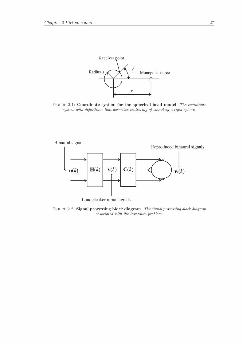
The signal processing block diagram associated with the inversion problem is illustratedin Figure 2.2, where C(k) is the matrix of transfer functions in the frequency domainthat relates the vector of loudspeaker input signals v(k) to the vector of output signalsw(k) produced at the listener’s ears. This makes the signals produced the listener’s earsw(k) = C(k)v(k). In order to create the vector v(k) of loudspeaker input signals, thematrix of cross-talk cancellation filters H(k) are multiplied with the vector of binauralsignals u(k) such that v(k) = H(k)u(k). The binaural signals u(k) can be recordedor alternatively synthesised by convolving them with a pair of filters representing thetransfer functions between the ears of the listener and the virtual source. The filtersrepresenting the transfer functions for the virtual sound source can be derived froma measured HRTF database. The cross-talk cancellation matrix should ideally makecertain that the reproduced signals w(k) are a delayed version of u(k). The reproducedsignals w(k) should be made equal to the desired signals d(k) at the listeners ears, whered(k) = u(k)e−jω∆ (∆ represents the number of samples delay). It follows that
C(k)H(k) ≈ e−jω∆I (2.9)
where I is the identity matrix. The solution at each discrete frequency k for the cross-talk
Chapter 2 Virtual sound 13
cancellation matrix is, in principle, given by
H(k) ≈ C−1(k)e−jω∆ (2.10)
The transfer function matrix C(k) for a symmetric arrangement of two loudspeakersand the listener is given by
C(k) =
[C11(k) C12(k)C21(k) C22(k)
](2.11)
where C11(k) = C22(k) and C21(k) = C12(k) are respectively, the frequency responsesat the direct and the cross-talk paths. The inverse matrix of C(k) is given by
C−1(k) =1
C211(k)− C2
21(k)
[C11(k) −C21(k)−C21(k) C11(k)
](2.12)
writing the ratio of the cross-talk to the direct paths as R(k) = C11(k)/C21(k) resultsin the following expression
C−1(k) =1
C11(k)(1−R(k))(1 + R(k))
[1 −R(k)
−R(k) 1
](2.13)
Assuming that the two transmission paths are governed only by the propagation delayand amplitude reduction associated with the spherical spreading of sound from a pointmonopole source as defined by Equation 2.1, such that
C11(k) =ρ0e
−jωr11/c0
4πr11(2.14)
C21(k) =ρ0e
−jωr21/c0
4πr21(2.15)
then we may write R(k) = ge−jωτ where g = r21/r11 is the ratio of the two path lengthsand τ = (r21 − r11)/c0 is the difference between the acoustic travel times from one ofthe loudspeakers to the furthest and nearest ears of the listener.
This shows that it is in principle possible to realise the matrix H(k) of cross-talk cancel-lation filters. The only component that can not be realisable in Equation 2.13 is the term1/C11(k). Hence, the need for a modelling delay, which is introduced into the numeratorof the solution for H(k) by the term e−jω∆ and provided the delay ∆ exceeds r11/c0
then there is no need to implement a time advance. In the inverse filters, the terms
Chapter 2 Virtual sound 14
R(k) appearing in the numerator of Equation 2.13 are realisable since they representpure delays and the terms 1/(1 + R(k)) and 1/(1 − R(k)) could also be realisable indiscrete time as recursive filters. However, there is a potential difficulty with Equation2.13 caused by the modulus squared of the filters appearing in the denominator i.e.
|1−R(k)|2 = (1 + g − 2 cos(ωτ)), |1 + R(k)|2 = (1 + g + 2 cos(ωτ)) (2.16)
The ratio of g will be close to unity and these terms will become small as the frequencyω tends to zero and at frequencies where cos(ωτ) = 1 or −1 respectively. This occurswhen
ωτ =2πf∆r
c0= nπ (2.17)
where n is an integer. This integer number should not be confused with the discrete timesample n. At these frequencies the response of the filters in Equation 2.13 becomes largeand the frequency at which ωτ = π or f = 1/2τ being the “ringing frequency” identifiedby Kirkeby [49]. The ringing frequency is associated with an undesirable response in thetime domain.
Under the condition that ∆h is small compared to the distance r (r >> ∆h), thepath-length difference ∆r is given by,
∆r = r11 − r21 = 4∆h sin(θ) (2.18)
Note that at asymmetric listener positions, the path-length difference becomes
∆r =12
(r12 + r21 − r11 − r22) (2.19)
The ill-conditioned and well-conditioned frequencies can be written as a function ofsource span 2θ and integer n by combining Equation 2.17 and 2.18. When n is anodd number represents well-conditioned frequencies and n even number represents ill-conditioned frequencies such that
f =nc0
8∆h sin(θ)(2.20)
Figure 2.9 illustrates the relationship between source span 2θ and frequency for differentodd integer numbers n.
The condition number of the plant matrix in the free field case can be compared tothe condition number of the plant matrix in the HRTF case. It can be shown that
Chapter 2 Virtual sound 15
by varying the receiver distance parameter ∆h, the free field model can be adjustedto a better approximation of the HRTF model (Takeuchi [97]). The receiver distancecorresponds to the shortest distance between the entrances of the ear canals of theKEMAR dummy head. The plant matrix of the HRTF model is similar to that of thefree field model with a receiver distance of 2∆h = 0.13 m where the incidence angle θ issmall, which corresponds to the shortest distance between the ear canals of the KEMARdummy head. Likewise, the plant matrix of the HRTF model is similar to that of thefree field model with a receiver distance of 2∆h = 0.25 m where the incidence angle θ
is large. This is a significantly larger distance than the shortest distance between theentrances of the ear canals of the KEMAR dummy head and is likely to be caused bydiffraction around the head. The receiver distance can for example be modeled to be alinear function of incident angle as in the simulations in Section 2.4.1.
2.2.1 Matrix inversion, SVD and regularisation
It is common practice to use regularisation for dealing with ill-conditioned inversionproblems (Kirkeby [51], Nelson [76]). An optimal solution for the vector v(k) is the onethat minimizes the sum of the squares of the errors e(k) = (d(k) −w(k)) between thedesired signals d(k) and the reproduced signals w(k). The solution to this optimisationproblem (Nelson and Elliott [72]) is given by the optimal loudspeaker input signals asfollows
vopt(k) =[CH(k)C(k) + βI
]−1CH(k)d(k) (2.21)
where β is the regularisation parameter. Given that d(k) = u(k)e−jω∆ the cross-talkcancellation matrix in Equation 2.9 can be written in terms of the pseudo-inverse matrix[CH(k)C(k) + βI
]−1 CH(k), such that,
HR(k) =[CH(k)C(k) + βI
]−1CH(k)e−jω∆ (2.22)
Using the singular value decomposition (SVD) of the matrix C(k) which can be writtenas
C(k) = UΣVH (2.23)
where U and VH are the unitary matrices of the left and right singular vectors, respec-tively, the superscript H denotes the Hermitian (complex conjugate) transpose and Σ isthe diagonal matrix of singular values. Substituting into this solution gives the followingsolution
Chapter 2 Virtual sound 16
HR(k) = V[ΣHΣ + βI
]−1ΣHUHe−jω∆ (2.24)
Using the free-field two-source two-field point model described above results in
[ΣHΣ + βI
]−1ΣH =
|1+R(k)||1+R(k)|2+β
0
0 |1−R(k)||1−R(k)|2+β
(2.25)
and this shows that the regularisation parameter limits the magnitude of the cross-talkcancellation filters at the particular frequencies where the terms |1 + R(k)| or |1−R(k)|become small.
2.2.2 Realisability of inverse filters
The transfer function to be inverted C(k) is naturally non-minimum phase where zerosappear outside the unit circle in the complex z-plane. The term 1/C(k) will then beunstable since zeros outside the unit circle become poles of the inverse filter. However,the poles outside the unit circle can also be interpreted as contributing to a stable butanti-causal component of the impulse response of the inverse filter [76]. The impulseresponse c(n) associated with the transfer function C(k) (using for example the sphericalhead model described in Section 2.1.2) can be described in terms of the z-transform
C(z) = z−qB(z) (2.26)
B(z) = b0 + b1z−1 + b2z
−2 + b3z−3 + . . . + bN−1z
−(N−1) (2.27)
where B(z) is a polynomial q and denotes the number of samples delay. The numberof coefficients used to represent the impulse response is denoted N . The terms bn arenon-zero values of the impulse response c(n). Now the transfer function B(z) can befactored into a product as
B(z) = b0(1− z1z−1)(1− z2z
−2) · · · (1− zNz−N ) (2.28)
where zi represent the zeros of the polynomial B(z). The inverse of B(z) can be writtenas a partial fraction expansion such as
B−1(z) =A1
(1− z1z−1)+
A2
(1− z2z−2)+ · · ·+ AN
(1− zNz−N )(2.29)
Chapter 2 Virtual sound 17
The poles of this expression are assumed to be distinct and it can be shown (Proakis [84])that when the inverse z-transform is evaluated, then the time domain sequence will bedetermined by the position of each relevant zero zi relative to the unit circle |z| = 1.When zeros are placed inside the unit circle, the inverse z-transform results in a causalsequence that decays exponentially in forward time. When zeros are placed outsidethe unit-circle, it can be argued that the inverse z-transform results in an anti-causalsequence of infinite duration in backward time. When zeros lie on the unit circle, theresulting sequence will be of infinite duration in either forward or backward time. Hence,the closer the zero is to the unit circle, the slower the rate of decay of the impulseresponse. To overcome this it was shown by Kirkeby [50] that a regularised solution forthe cross-talk cancellation matrix HR(k) can deal with inverting a non-minimum phasesystem. The rate of decay of the impulse responses of the inverse filters can successfullybe controlled by the regularisation parameter β that replaces each zero with a pair ofzeros that are each further away from the unit circle in the z-plane (Nelson [76]). Thiswill ensure that the response is sufficiently short compared to the length of the discreteFourier transform used, hence the effects of “wrap around” errors are also minimized.
The effectiveness of cross-talk cancellation can be evaluated using the “control perfor-mance” matrix given by the product C(k)HR(k).
P(k) = C(k)HR(k) =
[P11(k) P12(k)P21(k) P22(k)
](2.30)
Perfect cross-talk cancellation would result in unit values of P11(k) and P22(k) and zerovalues of P12(k) and P21(k). The impulse responses p(n) is found by taking the inverseFourier transform of the elements of P(k), and perfect cross-talk cancellation would thenresult in a Dirac impulse for p11(n) and p22(n) and zero values for p12(n) and p21(n).
p(n) =
[p11(n) p12(n)p21(n) p22(n)
](2.31)
It can be demonstrated that the reduction in gain of the cross-talk cancellation filtersthat is produced by increasing the regularisation factor β results in a deterioration inperformance as one might expect. There is a trade off between “control performance”and “control effort” that can be adjusted through the choice of regularisation factor.
Chapter 2 Virtual sound 18
2.3 Principles of the Stereo Dipole and the Optimal Source
Distribution
The performance of the virtual sound imaging system depends partly on the source spanas a function of frequency as described by Equation 2.20. The best control performanceis achieved when n is an odd integer number as demonstrated Figure 2.9 (Takeuchi [97]).Ideally the source span varies continuously as a function of frequency in order to satisfythe requirement for n to be an odd integer number as in Equation 2.20. The choice ofvalue for n is usually n = 1 since this gives the best low frequency control performanceand also results in control over the sound field up to frequencies above 20 kHz (with a∆h = 0.13 m as for the KEMAR dummy head). The smallest source span is approx-imately 4 and the widest source span is 180. The low frequency limit for optimalcontrol of the sound field is about 300-400 Hz (n = 1) when the distance between theears is 0.13 m.
The idea of using a loudspeaker with a source span that varies continuously as a functionfrequency is not feasible to implement in practice. A feasible solution is to discretise thesource span. The plant matrix is well conditioned in a relatively wide frequency regionaround the optimal frequency. Therefore, one can allow n to have some width, forexample ±ν, 0 < ν < 1, which results only in a small reduction of control performance.This can be interpreted as using the well-conditioned frequencies only and excluding ill-conditioned frequencies by limiting the frequency range to be used for a certain sourcespan. It is possible to build a practical system that covers most of the audible frequencyrange with a few sets of sources with different source spans.
An example of a 3-way OSD system is illustrated in Figure 2.5. The aim with the systemis to ensure a condition number that is as small as possible over a frequency range thatis as wide as possible. Therefore, the source spans were chosen at the extreme positionsfor the high frequency and low frequency limits. The high frequency limit is set to 20kHz and the low frequency limit is depicted by the maximum source span of 180. Thisgives ν = 0.7 and the source spans becomes 6.2 for the high frequency units, 32 forthe mid frequency units and 180 for the low frequency units as presented in Figure 2.6.The high frequency units (6.2) covers the frequency range up to 20 kHz for n+ν = 1.7.The low frequency limit of the low frequency units is about 110 Hz for n− ν = 0.3. Thecross-over frequencies are given by n − ν = 0.3 and n + ν = 1.7 for each pair of unitsand are located at 600 Hz and 4 kHz.
An example of a 2-way OSD system is illustrated in Figure 2.7. The aim with this systemis again to ensure a condition number that is as small as possible over a frequency rangeas wide as possible. The source spans are chosen to be 6.9 and 120, which givesν = 0.9. The mid-high frequency units (6.9) covers the frequency range up to 20 kHz(n + ν = 1.9). The low-mid frequency units covers the frequency range from about 40
Chapter 2 Virtual sound 19
Hz (n− ν = 0.1) up to the cross-over frequency at 900 Hz. The cross-over frequency isgiven by n − ν = 0.1 and n + ν = 1.9 for each pair of units. The condition number ofthe 2-way OSD system is illustrated in Figure 2.8.
By using a larger number of sources, i.e. a 4-way OSD system or 5-way OSD systemfor example, the smaller the width of n(±ν) becomes. In this evaluation a value of0.1 < n±ν < 1.9 is chosen, with the motivation that by allowing the listener to move androtate (azimuth angle), degradation in performance must be allowed and it is reasonableto accept a degradation from a 3-way OSD system (with 0.3 < n± ν < 1.7) down to a2-way OSD system (0.1 < n± ν < 1.9). Hence, at the worst listener position, the 3-wayOSD system will perform as the 2-way OSD system at its optimal position (on-axis andwith azimuth angle φ = 0 ) in terms of the condition number of the transfer functionmatrix. The SD system investigated below is also using the interval of 0.1 < n±ν < 1.9for comparative purposes.
2.4 Condition number for the inversion problem
The analytical solution of the two source-two field point inversion problem is presentedby Nelson [71], [76], for the free-field model and spherical head model respectively. The“ringing frequency” is associated with ill-conditioning of the frequency response functionmatrix to be inverted and results in a complex sound field at the listeners ears in thetime domain and a reduction in the size of the “sweet-spot”. The condition numberof the matrix C(k) is defined in terms of the singular value decomposition (SVD) ofthe matrix, as described in Equation 2.23. The condition number κ(C) of the matrixC(k) is given by the ratio of the maximum to minimum singular values that comprisethe elements of the diagonal of the matrix Σ. The condition number is a well-knownparameter in dealing with matrix inversion problems (Golub [32]). If the loudspeakerinput signals v(k) are determined from the solution for the cross-talk cancellation matrixin Equation 2.10, then it follows that,
v(k) = C−1(k)d(k) = C−1(k)u(k)e−jω∆ (2.32)
It can be shown that [32] the errors δv(k) in the solution for v(k) are related to the errorsδC(k) in the specification of the matrix C(k) and the errors δd(k) in the specificationof the desired signals d(k) by the inequality
‖δv(k)‖‖v(k)‖ ≤ κ(C)
[‖δC(k)‖‖C(k)‖ +
‖δd(k)‖‖d(k)‖
](2.33)
In Equation 2.33, the symbol ‖‖ denotes the 2-norm, which is the sum of the squaredelements of a vector or the square root of the largest singular value of a matrix. The error
Chapter 2 Virtual sound 20
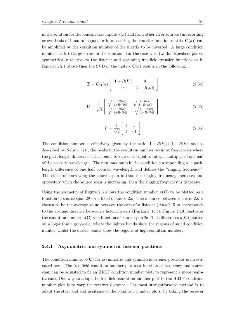
in the solution for the loudspeaker inputs v(k) and from other error sources (in recordingor synthesis of binaural signals or in measuring the transfer function matrix C(k)) canbe amplified by the condition number of the matrix to be inverted. A large conditionnumber leads to large errors in the solution. For the case with two loudspeakers placedsymmetrically relative to the listener and assuming free-field transfer functions as inEquation 2.1 above then the SVD of the matrix C(k) results in the following,
Σ = C11(k)
[|1 + R(k)| 0
0 |1−R(k)|
](2.34)
U =1√2
√|1+R(k)||1+R∗(k)|
√|1−R(k)||1−R∗(k)|√
|1+R(k)||1+R∗(k)| −
√|1−R(k)||1−R∗(k)|
(2.35)
V =1√2
[1 11 −1
](2.36)
The condition number is effectively given by the ratio |1 + R(k)| / |1−R(k)| and asdescribed by Nelson [71], the peaks in the condition number occur at frequencies wherethe path-length difference either tends to zero or is equal to integer multiples of one halfof the acoustic wavelength. The first maximum in the condition corresponding to a path-length difference of one half acoustic wavelength and defines the “ringing frequency”.The effect of narrowing the source span is that the ringing frequency increases andoppositely when the source span is increasing, then the ringing frequency is decreases.
Using the geometry of Figure 2.3 allows the condition number κ(C) to be plotted as afunction of source span 2θ for a fixed distance ∆h. The distance between the ears ∆h ischosen to be the average value between the ears of a listener (∆h=0.15 m correspondsto the average distance between a listener’s ears (Burkard [16])). Figure 2.10 illustratesthe condition number κ(C) as a function of source span 2θ. This illustrates κ(C) plottedon a logarithmic greyscale, where the lighter bands show the regions of small conditionnumber whilst the darker bands show the regions of high condition number.
2.4.1 Asymmetric and symmetric listener positions
The condition number κ(C) for asymmetric and symmetric listener positions is investi-gated here. The free field condition number plot as a function of frequency and sourcespan can be adjusted to fit an HRTF condition number plot, to represent a more realis-tic case. One way to adapt the free field condition number plot to the HRTF conditionnumber plot is to vary the receiver distance. The most straightforward method is toadapt the start and end positions of the condition number plots, by taking the receiver
Chapter 2 Virtual sound 21
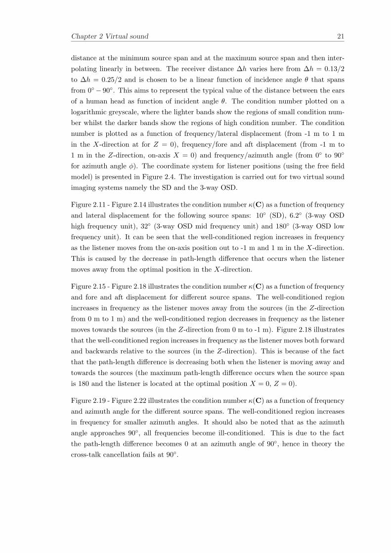
distance at the minimum source span and at the maximum source span and then inter-polating linearly in between. The receiver distance ∆h varies here from ∆h = 0.13/2to ∆h = 0.25/2 and is chosen to be a linear function of incidence angle θ that spansfrom 0− 90. This aims to represent the typical value of the distance between the earsof a human head as function of incident angle θ. The condition number plotted on alogarithmic greyscale, where the lighter bands show the regions of small condition num-ber whilst the darker bands show the regions of high condition number. The conditionnumber is plotted as a function of frequency/lateral displacement (from -1 m to 1 min the X-direction at for Z = 0), frequency/fore and aft displacement (from -1 m to1 m in the Z-direction, on-axis X = 0) and frequency/azimuth angle (from 0 to 90
for azimuth angle φ). The coordinate system for listener positions (using the free fieldmodel) is presented in Figure 2.4. The investigation is carried out for two virtual soundimaging systems namely the SD and the 3-way OSD.
Figure 2.11 - Figure 2.14 illustrates the condition number κ(C) as a function of frequencyand lateral displacement for the following source spans: 10 (SD), 6.2 (3-way OSDhigh frequency unit), 32 (3-way OSD mid frequency unit) and 180 (3-way OSD lowfrequency unit). It can be seen that the well-conditioned region increases in frequencyas the listener moves from the on-axis position out to -1 m and 1 m in the X-direction.This is caused by the decrease in path-length difference that occurs when the listenermoves away from the optimal position in the X-direction.
Figure 2.15 - Figure 2.18 illustrates the condition number κ(C) as a function of frequencyand fore and aft displacement for different source spans. The well-conditioned regionincreases in frequency as the listener moves away from the sources (in the Z-directionfrom 0 m to 1 m) and the well-conditioned region decreases in frequency as the listenermoves towards the sources (in the Z-direction from 0 m to -1 m). Figure 2.18 illustratesthat the well-conditioned region increases in frequency as the listener moves both forwardand backwards relative to the sources (in the Z-direction). This is because of the factthat the path-length difference is decreasing both when the listener is moving away andtowards the sources (the maximum path-length difference occurs when the source spanis 180 and the listener is located at the optimal position X = 0, Z = 0).
Figure 2.19 - Figure 2.22 illustrates the condition number κ(C) as a function of frequencyand azimuth angle for the different source spans. The well-conditioned region increasesin frequency for smaller azimuth angles. It should also be noted that as the azimuthangle approaches 90, all frequencies become ill-conditioned. This is due to the factthe path-length difference becomes 0 at an azimuth angle of 90, hence in theory thecross-talk cancellation fails at 90.
Chapter 2 Virtual sound 22
2.5 Operational area and cross-over design techniques
The performance of virtual sound imaging systems is affected by the geometry of thesystem and the position/rotation of the listener. When the listener is moving awayfrom the optimal position then the condition number of the transfer function matrixwill change and the system performance will decrease. This is illustrated by showing thefrequency bands (n ± ν) as a function of listener position/rotation for the SD and the3-way OSD. The area of successful operation is named the “operational area” and is afunction of: frequency, listener position/rotation and n±ν. The ν value is a performancecriterion and can be chosen depending on the requirements of the application. The valueof ν is here chosen to be 0.9 in order to represent the optimal performance of a static 2-way OSD system. Hence, in principle the performance of the adaptive 3-way OSD withinthe operational area will be as good or better (depending on position/rotation) than theperformance of the 2-way OSD at its optimal listening position. The implication ofthe choosen performance criterion is that a low value of ν increases the robustness ofthe system with respect to head misalignment, which leads to improved sound sourcelocalisation performance (Takeuchi [96]). The aim is to show the size of the operationalarea and to find out whether the cross-overs need to be updated as a function of listenerposition and rotation or if they can stay fixed.
The relationship between frequency and lateral listener displacement together with fixedcross-over frequencies for the SD and the 3-way OSD are plotted in Figures 2.23 and 2.24.The “operational area” is here a function of frequency range and listener displacementin the lateral plane. The fixed upper cross-over frequencies are indicated by circles ofthe same colour as the plotted lines that represents the source spans and correspondsto n and n ± ν. Likewise, the fixed lower cross-over points are indicated by squares ofthe same colour as their associated source span. The operational area for the SD coversthe frequency band 1000-13700 Hz (compared with on-axis performance of 720-13700Hz) for displacement in the lateral plane between −1 ≤ X ≤ 1 m. The operationalarea for the 3-way OSD covers the frequency band 34-23200 Hz (compared with on-axisperformance of 34-23200 Hz) for displacement in the lateral plane between −1 ≤ X ≤ 1m. The fixed cross-over points for the SD and the 3-way OSD are presented in Table2.2. It can be seen that the cross-over points for the source spans of the 3-way OSDare overlapping each other and there is not much benefit of updating the cross-overs.Within the overlapping sections, the cross-over points can be chosen depending on, forexample, the transducer characteristics.
The relationship between frequency and fore and aft displacement of the listener togetherwith fixed cross-over points for the SD and the 3-way OSD are plotted in Figure 2.25 and2.26. The “operational area” in this case, is a function of frequency range and listenerdisplacement in the fore and aft plane. The fixed cross-over points are again indicatedby circles and squares of the same colour as the plotted lines that represents the source
Chapter 2 Virtual sound 23
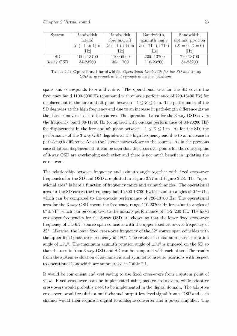
System Bandwidth, Bandwidth, Bandwidth, Bandwidth,lateral fore and aft azimuth angle optimal position
X (−1 to 1) m Z (−1 to 1) m φ (−71 to 71) (X = 0, Z = 0)[Hz] [Hz] [Hz] [Hz]
SD 1000-13700 1100-6900 2300-13700 720-137003-way OSD 34-23200 38-11700 110-23200 34-23200
Table 2.1: Operational bandwidth. Operational bandwidth for the SD and 3-wayOSD at asymmetric and symmetric listener positions.
spans and corresponds to n and n ± ν. The operational area for the SD covers thefrequency band 1100-6900 Hz (compared with on-axis performance of 720-13400 Hz) fordisplacement in the fore and aft plane between −1 ≤ Z ≤ 1 m. The performance of theSD degrades at the high frequency end due to an increase in path-length difference ∆r asthe listener moves closer to the sources. The operational area for the 3-way OSD coversthe frequency band 38-11700 Hz (compared with on-axis performance of 34-23200 Hz)for displacement in the fore and aft plane between −1 ≤ Z ≤ 1 m. As for the SD, theperformance of the 3-way OSD degrades at the high frequency end due to an increase inpath-length difference ∆r as the listener moves closer to the sources. As in the previouscase of lateral displacement, it can be seen that the cross-over points for the source spansof 3-way OSD are overlapping each other and there is not much benefit in updating thecross-overs.
The relationship between frequency and azimuth angle together with fixed cross-overfrequencies for the SD and OSD are plotted in Figure 2.27 and Figure 2.28. The “oper-ational area” is here a function of frequency range and azimuth angles. The operationalarea for the SD covers the frequency band 2300-13700 Hz for azimuth angles of 0±71,which can be compared to the on-axis performance of 720-13700 Hz. The operationalarea for the 3-way OSD covers the frequency range 110-23200 Hz for azimuth angles of0 ± 71, which can be compared to the on-axis performance of 34-23200 Hz. The fixedcross-over frequencies for the 3-way OSD are chosen so that the lower fixed cross-overfrequency of the 6.2 source span coincides with the upper fixed cross-over frequency of32. Likewise, the lower fixed cross-over frequency of the 32 source span coincides withthe upper fixed cross-over frequency of 180. The result is a maximum listener rotationangle of ±71. The maximum azimuth rotation angle of ±71 is imposed on the SD sothat the results from 3-way OSD and SD can be compared with each other. The resultsfrom the system evaluation of asymmetric and symmetric listener positions with respectto operational bandwidth are summarised in Table 2.1.
It would be convenient and cost saving to use fixed cross-overs from a system point ofview. Fixed cross-overs can be implemented using passive cross-overs, while adaptivecross-overs would probably need to be implemented in the digital domain. The adaptivecross-overs would result in a multi-channel output low level signal from a DSP and eachchannel would then require a digital to analogue converter and a power amplifier. The
Chapter 2 Virtual sound 24
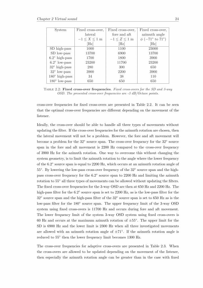
System Fixed cross-over, Fixed cross-over, Fixed cross-over,lateral fore and aft azimuth angle
−1 ≤ X ≤ 1 m −1 ≤ Z ≤ 1 m φ (−71 to 71)[Hz] [Hz] [Hz]
SD high-pass 1000 1100 23000SD low-pass 13700 6900 13700
6.2 high-pass 1700 1800 39006.2 low-pass 23200 11700 2320032 high-pass 280 300 65032 low-pass 3900 2200 3900
180 high-pass 34 38 110180 low-pass 650 650 650
Table 2.2: Fixed cross-over frequencies. Fixed cross-overs for the SD and 3-wayOSD. The presented cross-over frequencies are -3 dB/Octave points.
cross-over frequencies for fixed cross-overs are presented in Table 2.2. It can be seenthat the optimal cross-over frequencies are different depending on the movement of thelistener.
Ideally, the cross-over should be able to handle all three types of movements withoutupdating the filter. If the cross-over frequencies for the azimuth rotation are chosen, thenthe lateral movement will not be a problem. However, the fore and aft movement willbecome a problem for the 32 source span. The cross-over frequency for the 32 sourcespan in the fore and aft movement is 2200 Hz compared to the cross-over frequencyof 3900 Hz for the azimuth rotation. One way to overcome this without changing thesystem geometry, is to limit the azimuth rotation to the angle where the lower frequencyof the 6.2 source span is equal to 2200 Hz, which occurs at an azimuth rotation angle of55. By lowering the low-pass cross-over frequency of the 32 source span and the high-pass cross-over frequency for the 6.2 source span to 2200 Hz and limiting the azimuthrotation to 55 all three types of movements can be allowed without updating the filters.The fixed cross-over frequencies for the 3-way OSD are then at 650 Hz and 2200 Hz. Thehigh-pass filter for the 6.2 source span is set to 2200 Hz, as is the low-pass filter for the32 source span and the high-pass filter of the 32 source span is set to 650 Hz as is thelow-pass filter for the 180 source span. The upper frequency limit of the 3-way OSDsystem using fixed cross-overs is 11700 Hz and occurs during fore and aft movement.The lower frequency limit of the system 3-way OSD system using fixed cross-overs is60 Hz and occurs at the maximum azimuth rotation of ±55. The upper limit for theSD is 6900 Hz and the lower limit is 2300 Hz when all three investigated movementsare allowed with an azimuth rotation angle of ±71. If the azimuth rotation angle isreduced to 55 then the lower frequency limit becomes 1300 Hz.
The cross-over frequencies for adaptive cross-overs are presented in Table 2.3. Whenthe cross-overs are allowed to be updated depending on the movement of the listener,then especially the azimuth rotation angle can be greater than in the case with fixed
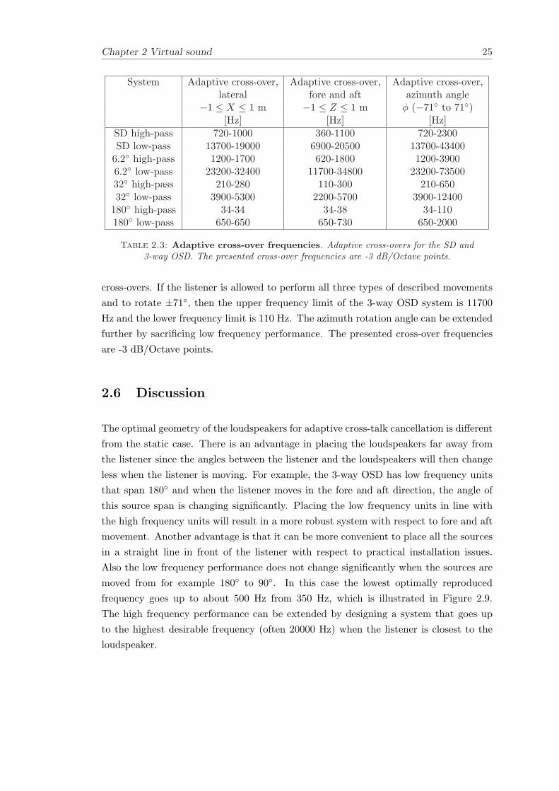
Chapter 2 Virtual sound 25
System Adaptive cross-over, Adaptive cross-over, Adaptive cross-over,lateral fore and aft azimuth angle
−1 ≤ X ≤ 1 m −1 ≤ Z ≤ 1 m φ (−71 to 71)[Hz] [Hz] [Hz]
SD high-pass 720-1000 360-1100 720-2300SD low-pass 13700-19000 6900-20500 13700-43400
6.2 high-pass 1200-1700 620-1800 1200-39006.2 low-pass 23200-32400 11700-34800 23200-7350032 high-pass 210-280 110-300 210-65032 low-pass 3900-5300 2200-5700 3900-12400
180 high-pass 34-34 34-38 34-110180 low-pass 650-650 650-730 650-2000
Table 2.3: Adaptive cross-over frequencies. Adaptive cross-overs for the SD and3-way OSD. The presented cross-over frequencies are -3 dB/Octave points.
cross-overs. If the listener is allowed to perform all three types of described movementsand to rotate ±71, then the upper frequency limit of the 3-way OSD system is 11700Hz and the lower frequency limit is 110 Hz. The azimuth rotation angle can be extendedfurther by sacrificing low frequency performance. The presented cross-over frequenciesare -3 dB/Octave points.
2.6 Discussion
The optimal geometry of the loudspeakers for adaptive cross-talk cancellation is differentfrom the static case. There is an advantage in placing the loudspeakers far away fromthe listener since the angles between the listener and the loudspeakers will then changeless when the listener is moving. For example, the 3-way OSD has low frequency unitsthat span 180 and when the listener moves in the fore and aft direction, the angle ofthis source span is changing significantly. Placing the low frequency units in line withthe high frequency units will result in a more robust system with respect to fore and aftmovement. Another advantage is that it can be more convenient to place all the sourcesin a straight line in front of the listener with respect to practical installation issues.Also the low frequency performance does not change significantly when the sources aremoved from for example 180 to 90. In this case the lowest optimally reproducedfrequency goes up to about 500 Hz from 350 Hz, which is illustrated in Figure 2.9.The high frequency performance can be extended by designing a system that goes upto the highest desirable frequency (often 20000 Hz) when the listener is closest to theloudspeaker.
Chapter 2 Virtual sound 26
2.7 Conclusion
It has been demonstrated that there is a relationship between cross-talk cancellationperformance for virtual sound imaging systems and the condition number of the matrixof transfer functions that needs to be inverted. The dependency of condition numberon frequency has been illustrated for the investigated asymmetric and symmetric lis-tener positions. An analytical model that estimates the “operational area” where the“sweet-spot” can be moved within for the adaptive SD and 3-way OSD system has beenpresented. The issue of using fixed or adaptive cross-overs has been investigated andrecommendations have been made. The use of fixed cross-overs will limit the azimuthrotation to 55, which can be compared to using adaptive cross-overs that allows for 71
azimuth rotation. The adaptive cross-over approach has not been used in this projectsince they create additional computational complexity in the signal processing scheme.However, they can improve the overall system performance and should be consideredfor implementation in future projects. The analytical evaluation presented here is com-plementary to the objective evaluation of the system performance in Chapter 5. Thenext chapter presents the measurement of a database of HRTFs, and the acquired datais used for the objective evaluations in Chapter 4 and Chapter 5.
Chapter 2 Virtual sound 27
r
Radius a
Receiver point
Monopole sourcef
Figure 2.1: Coordinate system for the spherical head model. The coordinatesystem with definitions that describes scattering of sound by a rigid sphere.
Loudspeaker input signals
Binaural signalsReproduced binaural signals
H( )k C( )k w( )kv( )ku( )k
Figure 2.2: Signal processing block diagram. The signal processing block diagramassociated with the inversion problem.
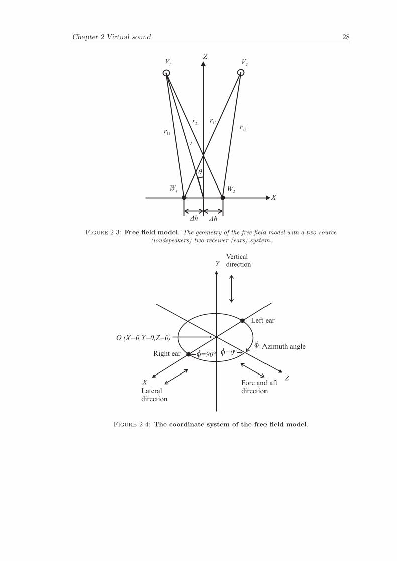
Chapter 2 Virtual sound 28
θ
Δh Δh
V1
V2
W2
W1
r
X
Z
r11
r21
r22
r12
Figure 2.3: Free field model. The geometry of the free field model with a two-source(loudspeakers) two-receiver (ears) system.
Azimuth angle
Lateraldirection
XZ
Fore and aftdirection
YVerticaldirection
=0°
O (X=0,Y=0,Z=0)
Left ear
Right ear =90°
fff
Figure 2.4: The coordinate system of the free field model.
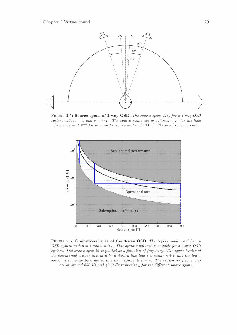
Chapter 2 Virtual sound 29
6.2º
32º
180º
Figure 2.5: Source spans of 3-way OSD. The source spans (2θ) for a 3-way OSDsystem with n = 1 and ν = 0.7. The source spans are as follows: 6.2 for the high
frequency unit, 32 for the mid frequency unit and 180 for the low frequency unit.
Sub−optimal performance
Sub−optimal performance
Operational area
Source span [°]
Fre
quen
cy [H
z]
0 20 40 60 80 100 120 140 160 180
102
103
104
Figure 2.6: Operational area of the 3-way OSD. The “operational area” for anOSD system with n = 1 and ν = 0.7. This operational area is suitable for a 3-way OSDsystem. The source span 2θ is plotted as a function of frequency. The upper border ofthe operational area is indicated by a dashed line that represents n + ν and the lowerborder is indicated by a dotted line that represents n − ν. The cross-over frequencies
are at around 600 Hz and 4000 Hz respectively for the different source spans.
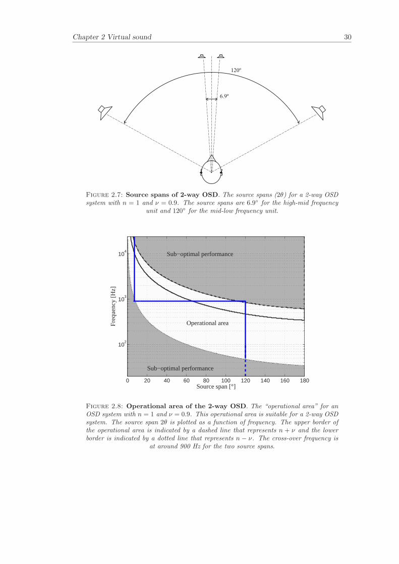
Chapter 2 Virtual sound 30
6.9º
120º
Figure 2.7: Source spans of 2-way OSD. The source spans (2θ) for a 2-way OSDsystem with n = 1 and ν = 0.9. The source spans are 6.9 for the high-mid frequency
unit and 120 for the mid-low frequency unit.
Sub−optimal performance
Sub−optimal performance
Operational area
Source span [°]
Fre
quen
cy [H
z]
0 20 40 60 80 100 120 140 160 180
102
103
104
Figure 2.8: Operational area of the 2-way OSD. The “operational area” for anOSD system with n = 1 and ν = 0.9. This operational area is suitable for a 2-way OSDsystem. The source span 2θ is plotted as a function of frequency. The upper border ofthe operational area is indicated by a dashed line that represents n + ν and the lowerborder is indicated by a dotted line that represents n − ν. The cross-over frequency is
at around 900 Hz for the two source spans.
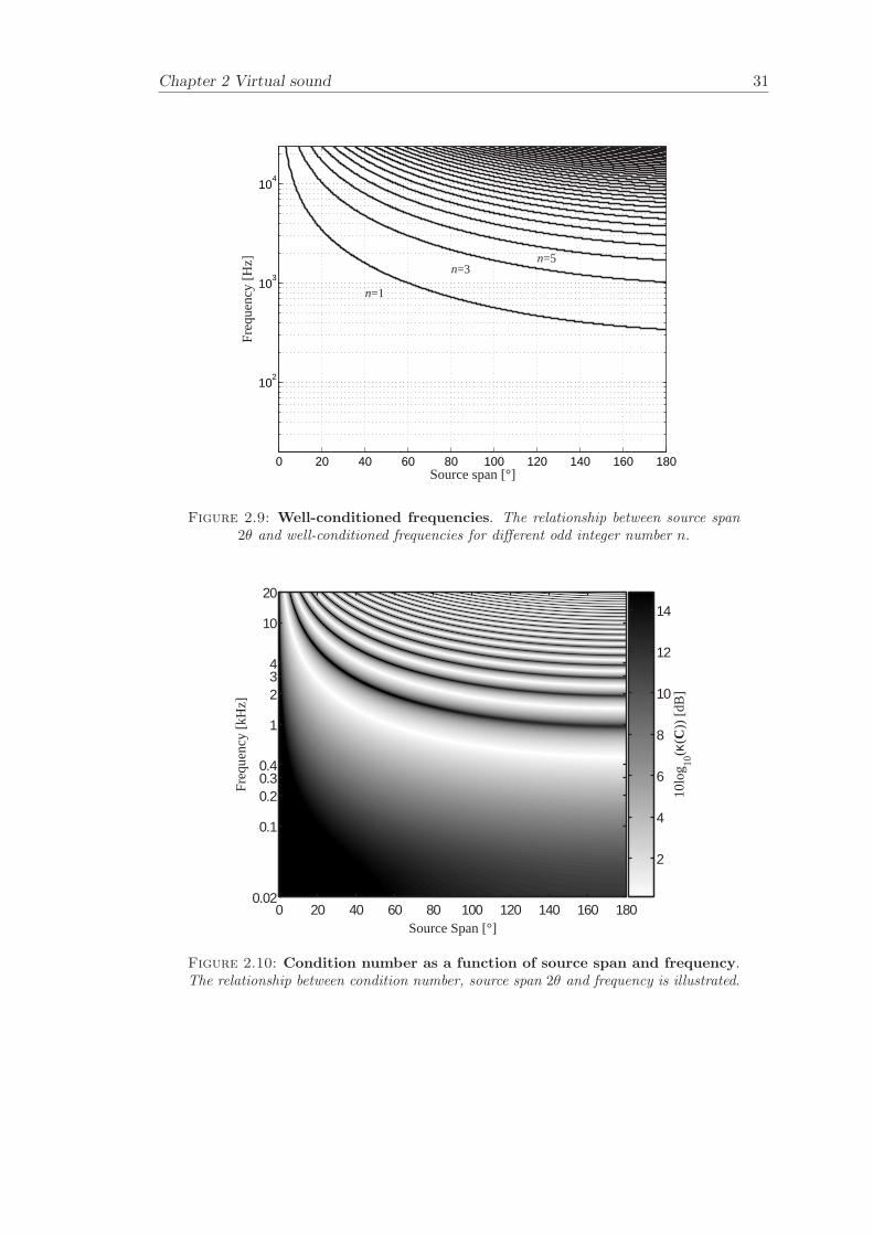
Chapter 2 Virtual sound 31
0 20 40 60 80 100 120 140 160 180
102
103
104
Source span [°]
Fre
quen
cy [H
z]
n=1
n=3n=5
Figure 2.9: Well-conditioned frequencies. The relationship between source span2θ and well-conditioned frequencies for different odd integer number n.
10lo
g 10(κ
(C))
[dB
]
2
4
6
8
10
12
14
Fre
quen
cy [k
Hz]
0 20 40 60 80 100 120 140 160 180Source Span [°]
0.02
0.1
0.20.30.4
1
234
10
20
Figure 2.10: Condition number as a function of source span and frequency.The relationship between condition number, source span 2θ and frequency is illustrated.
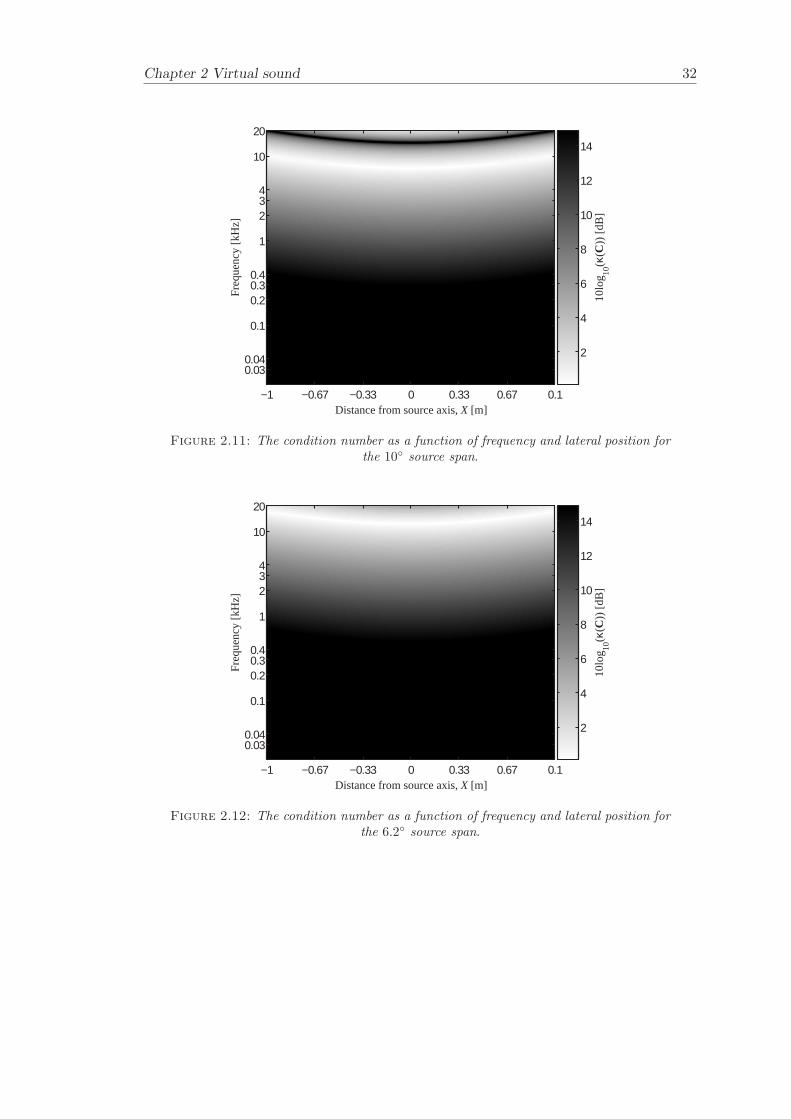
Chapter 2 Virtual sound 32
10lo
g 10(κ
(C))
[dB
]
2
4
6
8
10
12
14
Freq
uenc
y [k
Hz]
−1 −0.67 −0.33 0 0.33 0.67 0.1Distance from source axis, X [m]
0.030.04
0.1
0.20.30.4
1
234
10
20
Figure 2.11: The condition number as a function of frequency and lateral position forthe 10 source span.
10lo
g 10(κ
(C))
[dB
]
2
4
6
8
10
12
14
Freq
uenc
y [k
Hz]
−1 −0.67 −0.33 0 0.33 0.67 0.1Distance from source axis, X [m]
0.030.04
0.1
0.20.30.4
1
234
10
20
Figure 2.12: The condition number as a function of frequency and lateral position forthe 6.2 source span.
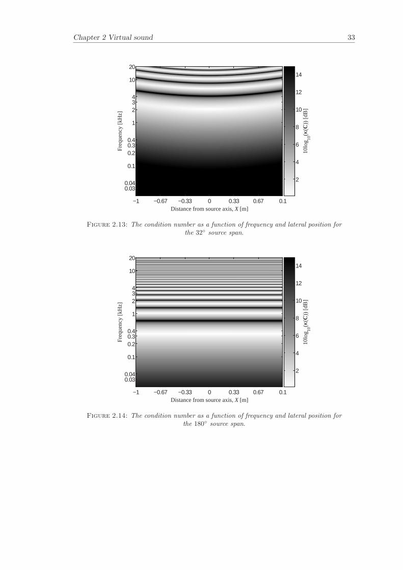
Chapter 2 Virtual sound 33
10lo
g 10(κ
(C))
[dB
]
2
4
6
8
10
12
14
Freq
uenc
y [k
Hz]
−1 −0.67 −0.33 0 0.33 0.67 0.1Distance from source axis, X [m]
0.030.04
0.1
0.20.30.4
1
234
10
20
Figure 2.13: The condition number as a function of frequency and lateral position forthe 32 source span.
10lo
g 10(κ
(C))
[dB
]
2
4
6
8
10
12
14
Freq
uenc
y [k
Hz]
−1 −0.67 −0.33 0 0.33 0.67 0.1Distance from source axis, X [m]
0.030.04
0.1
0.20.30.4
1
234
10
20
Figure 2.14: The condition number as a function of frequency and lateral position forthe 180 source span.
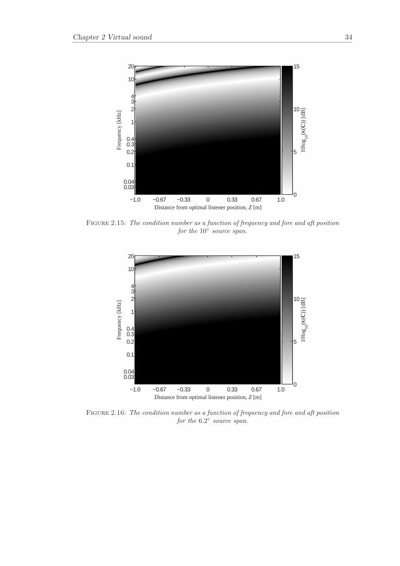
Chapter 2 Virtual sound 34
10lo
g 10(κ
(C))
[dB
]
0
5
10
15
Freq
uenc
y [k
Hz]
−1.0 −0.67 −0.33 0 0.33 0.67 1.0Distance from optimal listener position, Z [m]
0.030.04
0.1
0.20.30.4
1
234
10
20
Figure 2.15: The condition number as a function of frequency and fore and aft positionfor the 10 source span.
10lo
g 10(κ
(C))
[dB
]
0
5
10
15
Freq
uenc
y [k
Hz]
−1.0 −0.67 −0.33 0 0.33 0.67 1.0Distance from optimal listener position, Z [m]
0.030.04
0.1
0.20.30.4
1
234
10
20
Figure 2.16: The condition number as a function of frequency and fore and aft positionfor the 6.2 source span.
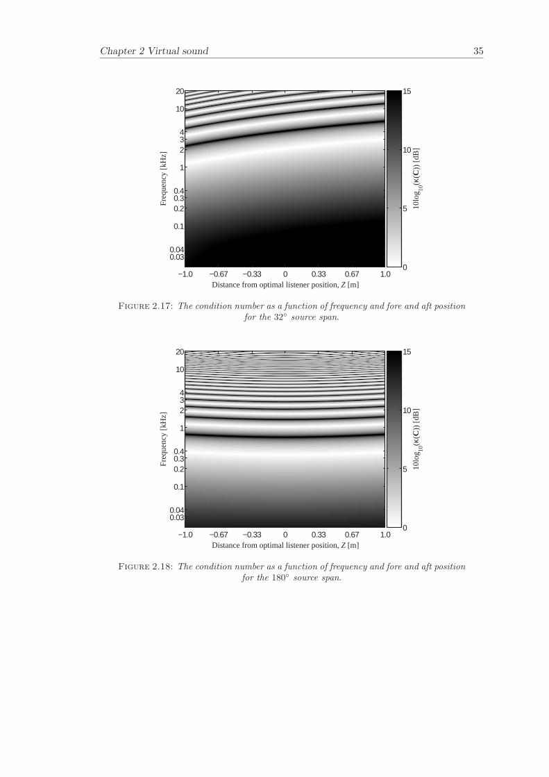
Chapter 2 Virtual sound 35
10lo
g 10(κ
(C))
[dB
]
0
5
10
15
Freq
uenc
y [k
Hz]
−1.0 −0.67 −0.33 0 0.33 0.67 1.0Distance from optimal listener position, Z [m]
0.030.04
0.1
0.20.30.4
1
234
10
20
Figure 2.17: The condition number as a function of frequency and fore and aft positionfor the 32 source span.
10lo
g 10(κ
(C))
[dB
]
0
5
10
15
Freq
uenc
y [k
Hz]
−1.0 −0.67 −0.33 0 0.33 0.67 1.0Distance from optimal listener position, Z [m]
0.030.04
0.1
0.20.30.4
1
234
10
20
Figure 2.18: The condition number as a function of frequency and fore and aft positionfor the 180 source span.
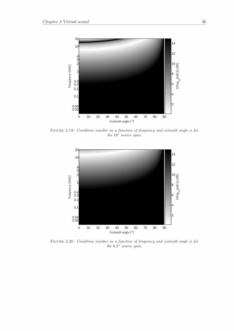
Chapter 2 Virtual sound 36
10lo
g 10(κ
(C))
(dB
)
2
4
6
8
10
12
14
Fre
quen
cy [k
Hz]
0 10 20 30 40 50 60 70 80 90Azimuth angle [°]
0.030.04
0.1
0.20.30.4
1
234
10
20
Figure 2.19: Condition number as a function of frequency and azimuth angle φ forthe 10 source span.
10lo
g 10(κ
(C))
(dB
)
2
4
6
8
10
12
14
Fre
quen
cy [k
Hz]
0 10 20 30 40 50 60 70 80 90Azimuth angle [°]
0.030.04
0.1
0.20.30.4
1
234
10
20
Figure 2.20: Condition number as a function of frequency and azimuth angle φ forthe 6.2 source span.
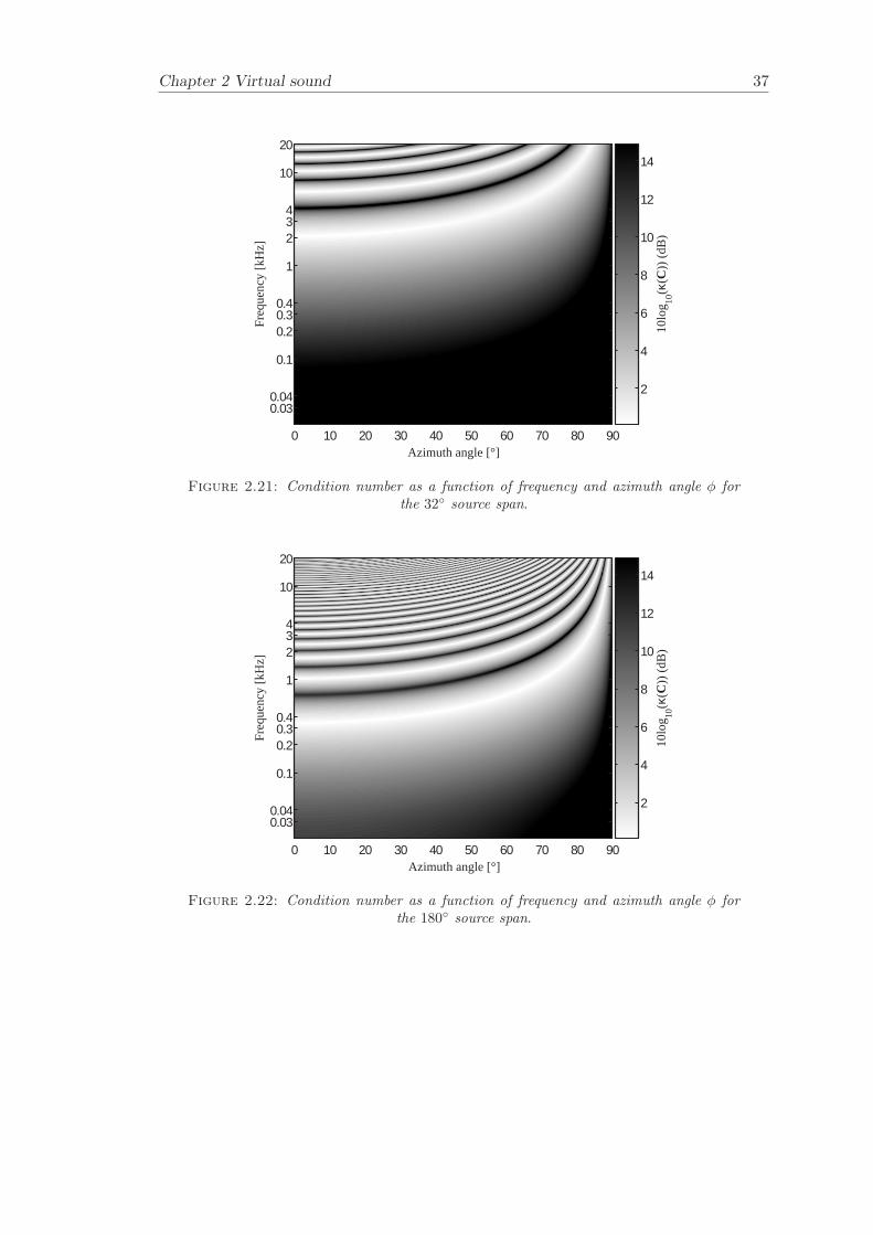
Chapter 2 Virtual sound 37
10lo
g 10(κ
(C))
(dB
)
2
4
6
8
10
12
14
Fre
quen
cy [k
Hz]
0 10 20 30 40 50 60 70 80 90Azimuth angle [°]
0.030.04
0.1
0.20.30.4
1
234
10
20
Figure 2.21: Condition number as a function of frequency and azimuth angle φ forthe 32 source span.
10lo
g 10(κ
(C))
(dB
)
2
4
6
8
10
12
14
Fre
quen
cy [k
Hz]
0 10 20 30 40 50 60 70 80 90Azimuth angle [°]
0.030.04
0.1
0.20.30.4
1
234
10
20
Figure 2.22: Condition number as a function of frequency and azimuth angle φ forthe 180 source span.
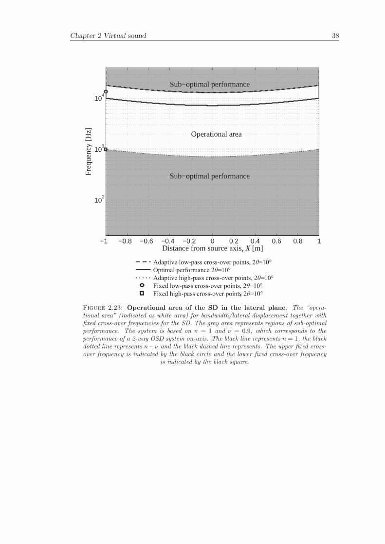
Chapter 2 Virtual sound 38
Sub−optimal performance
Sub−optimal performance
Operational area
Distance from source axis, X [m]
Fre
quen
cy [H
z]
−1 −0.8 −0.6 −0.4 −0.2 0 0.2 0.4 0.6 0.8 1
102
103
104
Adaptive low-pass cross-over points, 2 =10θ °
Optimal performance 2 =10θ °
Adaptive high-pass cross-over points, 2 =10θ °
Fixed low-pass cross-over points, 2 =10θ °
Fixed high-pass cross-over points, 2 =10θ °
Figure 2.23: Operational area of the SD in the lateral plane. The “opera-tional area” (indicated as white area) for bandwidth/lateral displacement together withfixed cross-over frequencies for the SD. The grey area represents regions of sub-optimalperformance. The system is based on n = 1 and ν = 0.9, which corresponds to theperformance of a 2-way OSD system on-axis. The black line represents n = 1, the blackdotted line represents n−ν and the black dashed line represents. The upper fixed cross-over frequency is indicated by the black circle and the lower fixed cross-over frequency
is indicated by the black square.
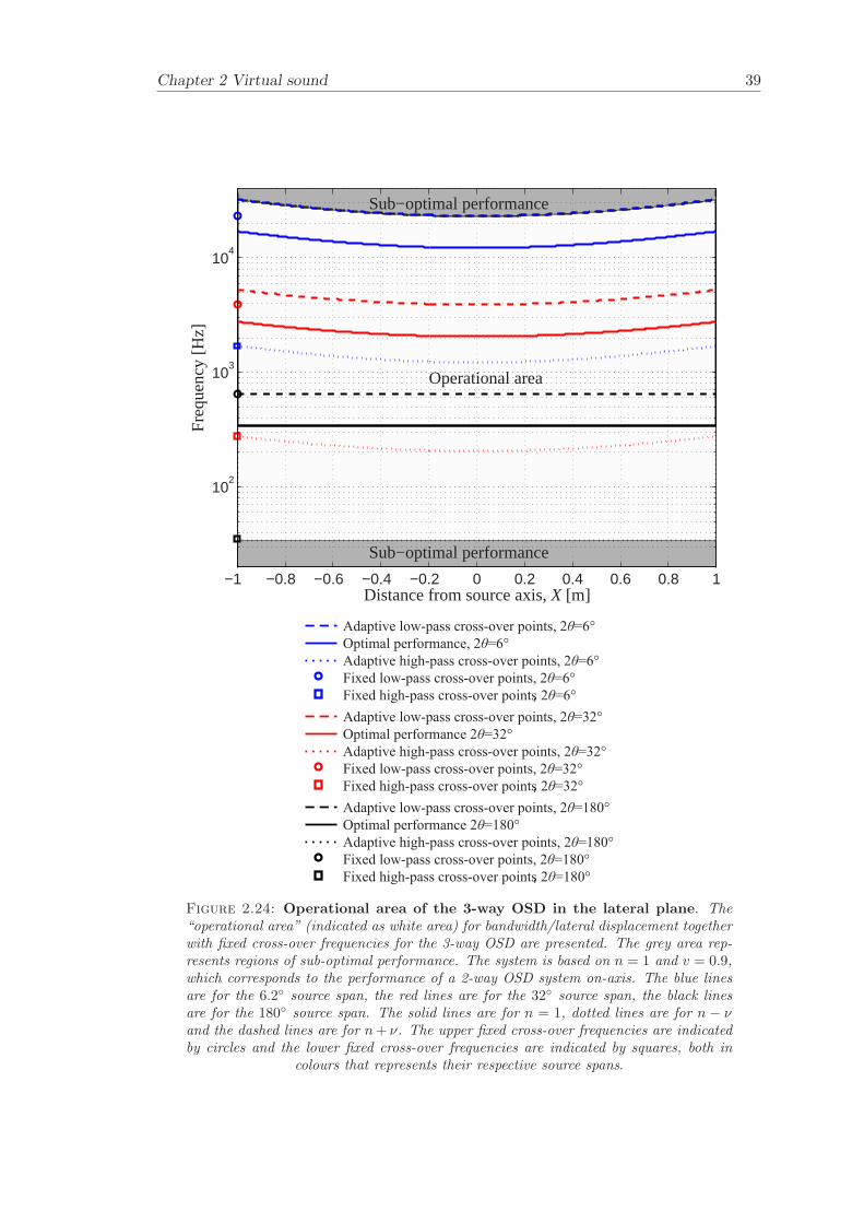
Chapter 2 Virtual sound 39
Distance from source axis, X [m]
Fre
quen
cy [H
z]
Sub−optimal performance
Sub−optimal performance
Operational area
−1 −0.8 −0.6 −0.4 −0.2 0 0.2 0.4 0.6 0.8 1
102
103
104
Adaptive low-pass cross-over points, 2 =6θ °
Optimal performance, 2 =6θ °
Adaptive -pass cross-over points,high 2 =6θ °
Fixed low-pass cross-over points, 2 =6θ °
Fixed -pass cross-over pointshigh , 2 =6θ °
Adaptive low-pass cross-over points, 2 =32θ °
Optimal performance 2 =32θ °
Adaptive -pass cross-over points,high 2 =32θ °
Fixed low-pass cross-over points, 2 =32θ °
Fixed -pass cross-over pointshigh , 2 =32θ °
Adaptive low-pass cross-over points, 2 =180θ °
Optimal performance 2 =180θ °
Adaptive -pass cross-over points,high 2 =180θ °
Fixed low-pass cross-over points, 2 =180θ °
Fixed -pass cross-over pointshigh , 2 =180θ °
Figure 2.24: Operational area of the 3-way OSD in the lateral plane. The“operational area” (indicated as white area) for bandwidth/lateral displacement togetherwith fixed cross-over frequencies for the 3-way OSD are presented. The grey area rep-resents regions of sub-optimal performance. The system is based on n = 1 and v = 0.9,which corresponds to the performance of a 2-way OSD system on-axis. The blue linesare for the 6.2 source span, the red lines are for the 32 source span, the black linesare for the 180 source span. The solid lines are for n = 1, dotted lines are for n − νand the dashed lines are for n + ν. The upper fixed cross-over frequencies are indicatedby circles and the lower fixed cross-over frequencies are indicated by squares, both in
colours that represents their respective source spans.
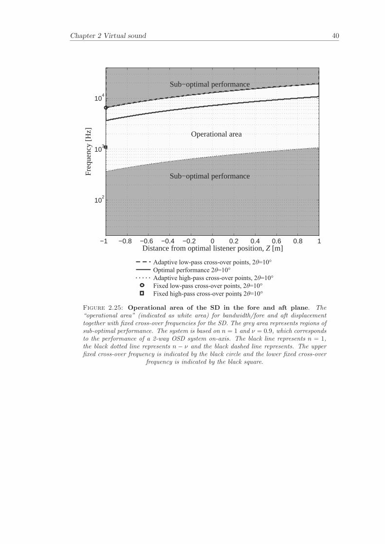
Chapter 2 Virtual sound 40
Sub−optimal performance
Sub−optimal performance
Operational area
Distance from optimal listener position, Z [m]
Fre
quen
cy [H
z]
−1 −0.8 −0.6 −0.4 −0.2 0 0.2 0.4 0.6 0.8 1
102
103
104
Adaptive low-pass cross-over points, 2 =10θ °
Optimal performance 2 =10θ °
Adaptive high-pass cross-over points, 2 =10θ °
Fixed low-pass cross-over points, 2 =10θ °
Fixed high-pass cross-over points, 2 =10θ °
Figure 2.25: Operational area of the SD in the fore and aft plane. The“operational area” (indicated as white area) for bandwidth/fore and aft displacementtogether with fixed cross-over frequencies for the SD. The grey area represents regions ofsub-optimal performance. The system is based on n = 1 and ν = 0.9, which correspondsto the performance of a 2-way OSD system on-axis. The black line represents n = 1,the black dotted line represents n − ν and the black dashed line represents. The upperfixed cross-over frequency is indicated by the black circle and the lower fixed cross-over
frequency is indicated by the black square.
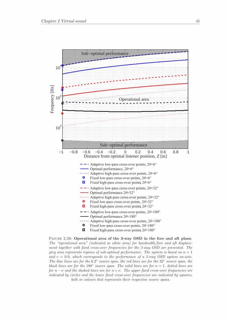
Chapter 2 Virtual sound 41
Distance from optimal listener position, Z [m]
Fre
quen
cy [H
z]
Sub−optimal performance
Sub−optimal performance
Operational area
−1 −0.8 −0.6 −0.4 −0.2 0 0.2 0.4 0.6 0.8 1
102
103
104
Adaptive low-pass cross-over points, 2 =6θ °
Optimal performance, 2 =6θ °
Adaptive -pass cross-over points,high 2 =6θ °
Fixed low-pass cross-over points, 2 =6θ °
Fixed -pass cross-over pointshigh , 2 =6θ °
Adaptive low-pass cross-over points, 2 =32θ °
Optimal performance 2 =32θ °
Adaptive -pass cross-over points,high 2 =32θ °
Fixed low-pass cross-over points, 2 =32θ °
Fixed -pass cross-over pointshigh , 2 =32θ °
Adaptive low-pass cross-over points, 2 =180θ °
Optimal performance 2 =180θ °
Adaptive -pass cross-over points,high 2 =180θ °
Fixed low-pass cross-over points, 2 =180θ °
Fixed -pass cross-over pointshigh , 2 =180θ °
Figure 2.26: Operational area of the 3-way OSD in the fore and aft plane.The “operational area” (indicated as white area) for bandwidth/fore and aft displace-ment together with fixed cross-over frequencies for the 3-way OSD are presented. Thegrey area represents regions of sub-optimal performance. The system is based on n = 1and v = 0.9, which corresponds to the performance of a 2-way OSD system on-axis.The blue lines are for the 6.2 source span, the red lines are for the 32 source span, theblack lines are for the 180 source span. The solid lines are for n = 1, dotted lines arefor n− ν and the dashed lines are for n + ν. The upper fixed cross-over frequencies areindicated by circles and the lower fixed cross-over frequencies are indicated by squares,
both in colours that represents their respective source spans.
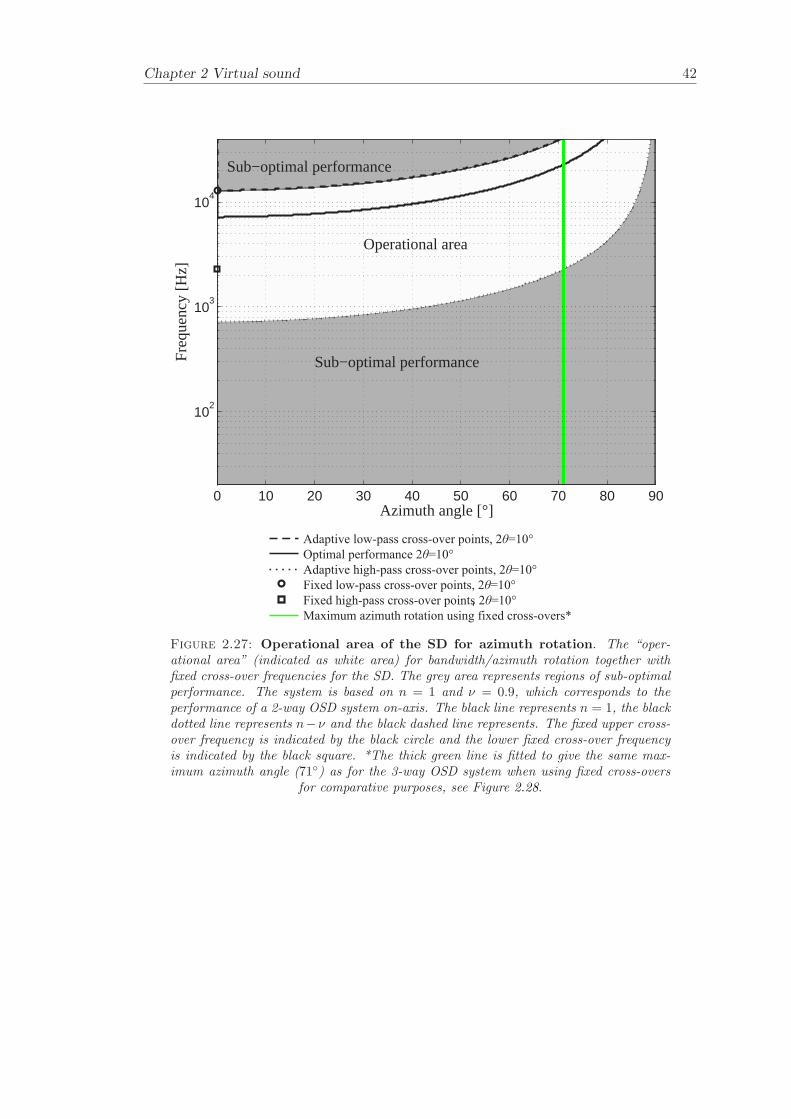
Chapter 2 Virtual sound 42
Sub−optimal performance
Sub−optimal performance
Operational area
Azimuth angle [°]
Fre
quen
cy [H
z]
0 10 20 30 40 50 60 70 80 90
102
103
104
Adaptive low-pass cross-over points, 2 =10θ °
Optimal performance 2 =10θ °
Adaptive high-pass cross-over points, 2 =10θ °
Fixed low-pass cross-over points, 2 =10θ °
Fixed high-pass cross-over points, 2 =10θ °
Maximum azimuth rotation using fixed cross-overs*
Figure 2.27: Operational area of the SD for azimuth rotation. The “oper-ational area” (indicated as white area) for bandwidth/azimuth rotation together withfixed cross-over frequencies for the SD. The grey area represents regions of sub-optimalperformance. The system is based on n = 1 and ν = 0.9, which corresponds to theperformance of a 2-way OSD system on-axis. The black line represents n = 1, the blackdotted line represents n−ν and the black dashed line represents. The fixed upper cross-over frequency is indicated by the black circle and the lower fixed cross-over frequencyis indicated by the black square. *The thick green line is fitted to give the same max-imum azimuth angle (71) as for the 3-way OSD system when using fixed cross-overs
for comparative purposes, see Figure 2.28.
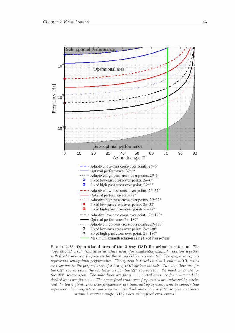
Chapter 2 Virtual sound 43
Azimuth angle [°]
Fre
quen
cy [H
z]
Sub−optimal performance
Sub−optimal performance
Operational area
0 10 20 30 40 50 60 70 80 90
102
103
104
Adaptive low-pass cross-over points, 2 =6θ °
Optimal performance, 2 =6θ °
Adaptive high-pass cross-over points, 2 =6θ °
Fixed low-pass cross-over points, 2 =6θ °
Fixed -pass cross-over pointshigh , 2 =6θ °
Adaptive low-pass cross-over points, 2 =32θ °
Optimal performance 2 =32θ °
Adaptive -pass cross-over points,high 2 =32θ °
Fixed low-pass cross-over points, 2 =32θ °
Fixed -pass cross-over pointshigh , 2 =32θ °
Adaptive low-pass cross-over points, 2 =180θ °
Optimal performance 2 =180θ °
Adaptive high-pass cross-over points, 2 =180θ °
Fixed low-pass cross-over points, 2 =180θ °
Fixed high-pass cross-over points, 2 =180θ °
Maximum azimuth rotation using fixed cross-overs
Figure 2.28: Operational area of the 3-way OSD for azimuth rotation. The“operational area” (indicated as white area) for bandwidth/azimuth rotation togetherwith fixed cross-over frequencies for the 3-way OSD are presented. The grey area regionsrepresents sub-optimal performance. The system is based on n = 1 and v = 0.9, whichcorresponds to the performance of a 2-way OSD system on-axis. The blue lines are forthe 6.2 source span, the red lines are for the 32 source span, the black lines are forthe 180 source span. The solid lines are for n = 1, dotted lines are for n− ν and thedashed lines are for n+ν. The upper fixed cross-over frequencies are indicated by circlesand the lower fixed cross-over frequencies are indicated by squares, both in colours thatrepresents their respective source spans. The thick green line is fitted to give maximum
azimuth rotation angle (71) when using fixed cross-overs.
Chapter 3
The measurement of a database
of head related transfer functions
Knowledge of HRTFs is essential in the synthesis of binaural signals, such as those usedin virtual reality applications. The measurement of arguably the most comprehensivedatabase to date of HRTFs of the KEMAR dummy head is presented here. The fea-tures of HRTFs are illustrated, such as the non-directional character of the propagationalong the ear canal and the HRTF measured without the pinna. The measurement wasconducted by the ISVR Samsung Joint Lab. An HRTF describes, for a certain angleof incidence, the sound transmission from a free field to a point in the ear canal of thesubject. The subject in this project is a KEMAR dummy head, which is used to modelan average human subject. The idea behind the binaural technique can be summarisedas follows. Spatial hearing relies on the two signals that comprise the sound pressureat the each of the ear drums. If these are recorded at the ears of the listener and arelater reproduced exactly, then the exact audio experience is recreated. The HRTF char-acterises the transfer function between source and the two ear signals and takes intoaccount the reflections and diffractions from the human torso, head and pinna.
The ISVR-Samsung measurement was performed on a KEMAR dummy head at 72 dif-ferent azimuth and 14 different angles of elevation giving a total of 1008 directions. Theazimuth angle resolution is 5 and the elevation angle resolution is 10. The samplingfrequency used is 48 kHz and the quantization depth is 24 bits. Pink noise was used toobtain the impulse responses. The data was saved as both equalized and raw data, wherethe length of the equalised HRIRs is 512 samples and the length of the raw HRIRs is4096 samples. The KEMAR dummy head measurements where performed for a “smallpinna”, “large pinna” and “no pinna”. The “small pinna” represents typical ears ofAmerican and European females as well as Japanese males and females. The “largepinna” represents typical ears of American and European males. The “no pinna” mea-surement is useful for modelling of HRTFs. The measurements were taken with both
44
Chapter 3 The measurement of a database of head related transfer functions 45
blocked and open ear canals for all the six cases and on both the left and the right ear.The measurement set-up for the ISVR Samsung data where performed in the anechoicchamber of the ISVR at a distance of 2 m between the loudspeakers and the centre ofthe listeners head. The aim of the measurement was also to provide a database withhigh sound quality by using 24 bit 48 kHz sampling frequency and high signal to noiseratio (SNR).
Previous measurements have been published in the literature such as those reported by,Moller [69], Gardner [31] at MIT, and Algazi et al [2] at CIPIC. These measurementsare briefly described here. The Moller [69] measurement was performed on 40 humansubjects for 97 directions of sound incidence, covering the entire sphere. IndividualHRTF data for the median, horizontal, and frontal planes are presented in the frequencydomain. The measurements were made synchronously at both ears. The measurementswere made at the entrance to a blocked ear canal and also at the entrance to an openear canal (by means of a probe microphone).
The MIT measurements consist of the left and right ear impulse responses from a loud-speaker mounted 1.4 m from the KEMAR dummy head. Maximum length pseudorandom binary sequences were used to obtain the impulse responses at a sampling rateof 44.1 kHz. In total 7200 different positions were sampled. The impulse response ofthe speaker in a free field and several headphones placed on the KEMAR were alsomeasured. The length of the HRIRs is 512 samples in the full database. Left-Rightsymmetry was assumed for KEMAR and hence all the right-ear responses were obtainedusing the “small pinna” model and all the left-ear responses with the “large pinna”model.
The CIPIC database measurement was performed on 45 subjects at 25 different azimuthsand 50 different elevations (1250 directions) at approximately 5 angular increments.The database also contains anthropometric parameters. The KEMAR dummy headis included in the 45 subjects for whom they have measured HRTFs. The samplingfrequency they used is 44.1 kHz and the length of the HRIRs is 200 samples. TheKEMAR measurements where performed on a blocked ear canal for the “small pinna”and “large pinna” on both the left and the right ear. The measurement set-up for theCIPIC data where performed in the CIPIC Interface laboratory at a distance of 1 mbetween the speaker and the centre of the listeners head.
3.1 Measurement arrangement and procedures
The equipment and procedures necessary for the HRTF measurements are presentedhere. The mechanism of the measurement rig that holds a set of 14 loudspeakers androtates the KEMAR in the azimuth direction is described in depth.
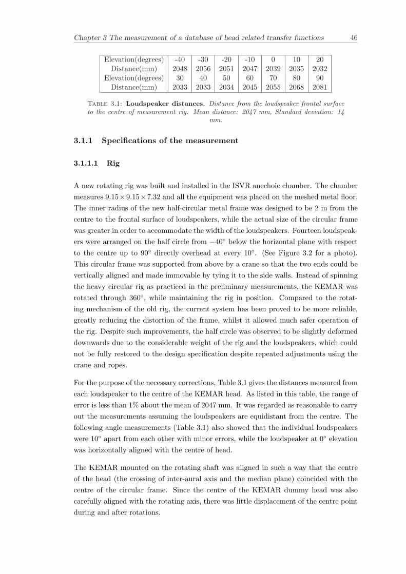
Chapter 3 The measurement of a database of head related transfer functions 46
Elevation(degrees) -40 -30 -20 -10 0 10 20Distance(mm) 2048 2056 2051 2047 2039 2035 2032
Elevation(degrees) 30 40 50 60 70 80 90Distance(mm) 2033 2033 2034 2045 2055 2068 2081
Table 3.1: Loudspeaker distances. Distance from the loudspeaker frontal surfaceto the centre of measurement rig. Mean distance: 2047 mm, Standard deviation: 14
mm.
3.1.1 Specifications of the measurement
3.1.1.1 Rig
A new rotating rig was built and installed in the ISVR anechoic chamber. The chambermeasures 9.15×9.15×7.32 and all the equipment was placed on the meshed metal floor.The inner radius of the new half-circular metal frame was designed to be 2 m from thecentre to the frontal surface of loudspeakers, while the actual size of the circular framewas greater in order to accommodate the width of the loudspeakers. Fourteen loudspeak-ers were arranged on the half circle from −40 below the horizontal plane with respectto the centre up to 90 directly overhead at every 10. (See Figure 3.2 for a photo).This circular frame was supported from above by a crane so that the two ends could bevertically aligned and made immovable by tying it to the side walls. Instead of spinningthe heavy circular rig as practiced in the preliminary measurements, the KEMAR wasrotated through 360, while maintaining the rig in position. Compared to the rotat-ing mechanism of the old rig, the current system has been proved to be more reliable,greatly reducing the distortion of the frame, whilst it allowed much safer operation ofthe rig. Despite such improvements, the half circle was observed to be slightly deformeddownwards due to the considerable weight of the rig and the loudspeakers, which couldnot be fully restored to the design specification despite repeated adjustments using thecrane and ropes.
For the purpose of the necessary corrections, Table 3.1 gives the distances measured fromeach loudspeaker to the centre of the KEMAR head. As listed in this table, the range oferror is less than 1% about the mean of 2047 mm. It was regarded as reasonable to carryout the measurements assuming the loudspeakers are equidistant from the centre. Thefollowing angle measurements (Table 3.1) also showed that the individual loudspeakerswere 10 apart from each other with minor errors, while the loudspeaker at 0 elevationwas horizontally aligned with the centre of head.
The KEMAR mounted on the rotating shaft was aligned in such a way that the centreof the head (the crossing of inter-aural axis and the median plane) coincided with thecentre of the circular frame. Since the centre of the KEMAR dummy head was alsocarefully aligned with the rotating axis, there was little displacement of the centre pointduring and after rotations.
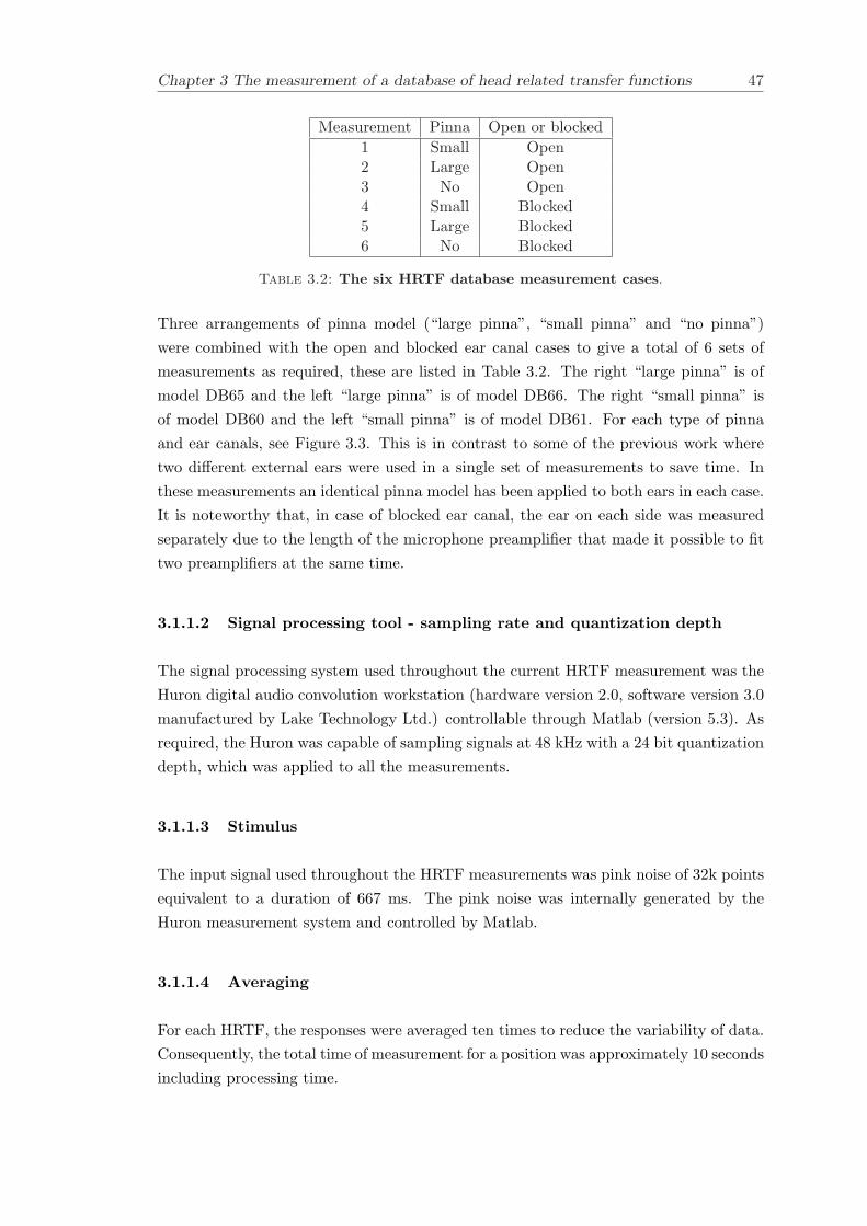
Chapter 3 The measurement of a database of head related transfer functions 47
Measurement Pinna Open or blocked1 Small Open2 Large Open3 No Open4 Small Blocked5 Large Blocked6 No Blocked
Table 3.2: The six HRTF database measurement cases.
Three arrangements of pinna model (“large pinna”, “small pinna” and “no pinna”)were combined with the open and blocked ear canal cases to give a total of 6 sets ofmeasurements as required, these are listed in Table 3.2. The right “large pinna” is ofmodel DB65 and the left “large pinna” is of model DB66. The right “small pinna” isof model DB60 and the left “small pinna” is of model DB61. For each type of pinnaand ear canals, see Figure 3.3. This is in contrast to some of the previous work wheretwo different external ears were used in a single set of measurements to save time. Inthese measurements an identical pinna model has been applied to both ears in each case.It is noteworthy that, in case of blocked ear canal, the ear on each side was measuredseparately due to the length of the microphone preamplifier that made it possible to fittwo preamplifiers at the same time.
3.1.1.2 Signal processing tool - sampling rate and quantization depth
The signal processing system used throughout the current HRTF measurement was theHuron digital audio convolution workstation (hardware version 2.0, software version 3.0manufactured by Lake Technology Ltd.) controllable through Matlab (version 5.3). Asrequired, the Huron was capable of sampling signals at 48 kHz with a 24 bit quantizationdepth, which was applied to all the measurements.
3.1.1.3 Stimulus
The input signal used throughout the HRTF measurements was pink noise of 32k pointsequivalent to a duration of 667 ms. The pink noise was internally generated by theHuron measurement system and controlled by Matlab.
3.1.1.4 Averaging
For each HRTF, the responses were averaged ten times to reduce the variability of data.Consequently, the total time of measurement for a position was approximately 10 secondsincluding processing time.
Chapter 3 The measurement of a database of head related transfer functions 48
3.1.2 Rig operation
3.1.2.1 Motorised turntable (azimuth)
As briefly described in Section 3.1.1.1, the half-circular metal frame was fixed and theKEMAR rotated about the vertical axis to which the two ends of the frame were aligned.This movement in azimuth was enabled by a motorized turntable engaged with a stepmotor by a chain, and the motor was operated by Matlab through a microcontroller.
3.1.2.2 Switch box (elevation)
Once the KEMAR was placed at a certain azimuth angle, HRTFs at each elevationwere measured by switching the input signal to the loudspeaker corresponding to eachelevation angle, instead of actually moving a loudspeaker along the circumference. Theswitch box that alternated the connections between the power amplifier and all the 14loudspeakers was controlled, again, by Matlab through the microcontroller.
3.1.3 Measurement equipment
3.1.3.1 Microphones
There were two kinds of microphones used throughout this measurement. One is B& K type 4134, and the other type 4136. The former was mounted on the Zwislockicoupler and used for the three cases of open ear canal, and the latter was used for theother three cases of blocked ear canal and the free field measurement. This is becausethe type 4134 of 0.5 inch diameter was too big to be fitted into the rubber pinna (seeFigure 3.3). Two 4134- and one 4136-microphones were calibrated using B & K 4230calibrator, and two measuring amplifiers used for each of the left and right channelswere tuned to indicate identical sound level. The sinusoidal signals captured during thecalibrations were also recorded for further corrections. The gain difference between two4134 microphones was about 0.05 dB, which is discountable on the dB scale, whilst the4136 microphone appeared about 17 dB less sensitive than one of the 4134 microphones.These gain differences were fully taken into account during the data processing later on.
3.1.3.2 Loudspeakers
The 14 loudspeakers (which were 4 inch paper cone drivers manufactured by Fostex) usedin the measurement were mounted in cabinets manufactured in the ISVR departmentalworkshop. There has been a concern about the size of these speakers that they mighthave higher cut-on frequencies, but the calibrations showed that they are reasonably
Chapter 3 The measurement of a database of head related transfer functions 49
reliable at low (down to 100 Hz) as well as at high frequencies. This can be regarded as ofless importance since, for the final HRTF database, the responses from the loudspeakersto the microphone on/in the ears will be deconvolved with the free field response of themicrophone and each loudspeaker. The characteristic response of the 14 loudspeakerswas reasonably identical up to 10-15 kHz and with a deviation of less than 2 dB.
3.1.3.3 Measuring amplifier and power amplifier
Two B & K 2636 measuring amplifiers have been used for each of the left and rightchannels throughout the measurement, and the left channel of a YAMAHA H5000 poweramplifier has driven the loudspeakers. Input/output gains were carefully chosen to avoidany clipping errors while maintaining acceptable signal levels.
3.1.3.4 SNR estimates
In advance of the full processing of the acquired data, a few responses were randomlychosen to investigate the SNR. This was evaluated by looking at the difference betweenone of the typical measurements and the measurement performed with all settings iden-tical, but with the loudspeaker replaced by an 8-ohm resistor (Moller [69]). The SNRmeasured for the left ear of the KEMAR at (φ = 0, ψ = 0) is in the range of 50-70dB except for the region of “pinna notch”. This SNR is found to be comparable to theprevious HRTF measurements introduced in the beginning of the chapter.
3.1.4 Measurement Procedure
All the measurement procedures and processes were controlled via Matlab commandsthat were written in a set of script files. Once the measurement equipment was calibratedand ready in the closed anechoic chamber, the rotating turntable and the switch boxwere initialized so that the KEMAR faced straight towards the array of loudspeakers(φ = 0), and the pink noise could be played from the loudspeaker at the lowest elevation(−40 elevation).
On completion of Huron recording the microphone output for the first angle, the pinknoise signal was switched to the next loudspeaker (elevation), and, after all the 14 eleva-tions were measured, the turntable rotated clockwise for the KEMAR to be positionedat 355 azimuth. In this way, 72 azimuth angles from 0 to 5 in −5 decrements (0,355, 350,, 10, 5) were measured for about 3 hours duration for each of the pinnamodels, and the recorded data were saved in the Matlab data format of a ’mat’ file.Finally, the free field transfer functions were measured for each loudspeaker (elevation)
Chapter 3 The measurement of a database of head related transfer functions 50
with the 4136 microphone held normal to the circular frame at its centre. These trans-fer functions will be used in the deconvolution process in order to obtain the responsefunctions resulting only from the existence of KEMAR.
3.2 Data processing
The data processing of the measurement conducted in July 2004 at the ISVR is presentedhere. Section 3.2.1 presents the coordinate system for how the data is presented. Section3.2.2 describes the equalization procedure used with the data and also how the data wasprocessed and stored. Section 3.2.3 discusses data processing operations and filter designissues.
3.2.1 Coordinate system
More than one convention exists in the literature as regards to the coordinate systemused for the description of the existing HRTF databases. In this thesis we use the sameconvention as that in the MIT database, in which the azimuth angles range from 0 to355 and the elevation angles from −90 to 90 degrees. In this sense: (φ = 0, ψ = 0)corresponds to the point directly ahead, (φ = 90, ψ = 0) corresponds to the pointdirectly to the right, (φ = 270, ψ = 0) corresponds to the point directly to the left,(φ = 0, ψ = 90) corresponds to the point directly on top and (φ = 180, φ = 0)corresponds to the point directly behind. The coordinate system is illustrated in Figure3.4. The figure shows the coordinate systems for the horizontal plane, the median planeand the frontal plane. The horizontal plane goes clockwise from 0 to 355 in 5 steps,which results in 72 azimuth angles. The median plane goes anti clockwise from −40 to90 (φ = 0) in 10 steps and from 90 to −40 (φ = 180), which results in 36 elevationangles. The frontal plane goes anti clockwise from −40 to 90 (φ = 90) in 10 stepsand from −40 to 90 (φ = 270), which results in 36 elevation angles.
3.2.2 Equalization procedure
The responses from the loudspeakers that were mounted on the measurement rig were allmeasured and in the data processing procedure the loudspeaker responses were decon-volved from the measured HRTFs. The responses from the loudspeakers were measuredwith a B & K type 4136 microphone, as described in section 3.1.3. The equalization wasundertaken by dividing the HRTF at each angle with the free field transfer function atthe respective angle (obtained by taking an FFT of the free field response). An inverseFFT was then applied in order to get back to the time domain. Finally an FFT shiftwas applied, so that the equalised HRIR could be obtained.
Chapter 3 The measurement of a database of head related transfer functions 51
The measurement on the blocked ear canal was made with the same microphone asthe free field measurement, and hence the equalization procedure takes account for theresponse of the measurement system in the blocked ear canal data. The equalizationof the open ear canal does not take into account the exact response of the system,since another type of microphone was used, namely the B & K type 4134. However thefrequency response of the microphones is similar and the equalization of the open earcanal with free field measurement is here considered as a good approximation.
The equalised HRTF data was saved in 72× 14× 2× 512 multi-dimensional arrays. Theequalised data was processed from the raw data arrays (72×14×2×4096). The raw dataholds the 4096 first points of the entire measurement series. Firstly the raw data waswindowed to 256 points with a rectangular window (points 301 - 556), in order to capturethe most essential information in the impulse response. The same windowing (points301 - 556) was applied to the free field impulse response. The two truncated impulseresponses are Fourier transformed with a 2048 point FFT and their ratio computed.This ratio was transformed back to the time-domain with an inverse FFT and a circularshift of the result which was then multiplied with a 2048 point Hanning window. 512points (974 -1486) of the obtained impulse response was kept.
3.2.3 Discussion
3.2.3.1 Specification of the data
According to the project specifications the acquired data is quantised to 24 bits andsampled at 48 kHz, which is a high definition audio format. Depending on the specificapplication in which it will be used, the database can be appropriately modified. A brieflist of potential modifications follows:
The size of the equalized data is 512 points and it may be desirable to change thesize of the data to, say, 256, 128, 64 or 32 points. The desired size of the impulseresponse is application dependent, where for example an MP3 player may have verylimited processing power and can only handle short impulse responses. The followingreferences Jot [44], [43], Algazi [3], Duda [27] and Blommer [14] give further details onefficient implementations of HRTFs. A comparison of digital filter design methods ispresented by Huopaniemi [39]. Filter design issues are also discussed in Chapter 5.
It is possible that the database has to be used for applications designed for differentsample rates. Data resampling (Proakis [84]) can be practically implemented withthe standard Matlab functions (e.g. resample.m Matlab [63]). The degree to whichsuch processing (especially down sampling) degrades the audio quality of the specificapplication should be verified by appropriate simulations and listening tests. If usedfor applications designed in shorter word-lengths (e.g. 16-bit) the appropriate use ofdithering should be considered.
Chapter 3 The measurement of a database of head related transfer functions 52
As is typical with measured HRTF databases, the responses in the ISVR Samsung HRTFdatabase are not of minimum phase. In case of a real-time filter application with HRTFs,the system designer needs to take account of the non-minimum phase characteristics.This will be particularly relevant in the case of designing inverse filters for cross-talkcancellation as described in Chapter 2.
3.2.3.2 Equalization comparison: MIT and ISVR
The equalization procedure in the ISVR database is similar to that used by MIT. Themain difference between the ISVR and the MIT database is that the MIT database iscompensated with the minimum phase representation of the free field impulse responsewhile the ISVR databse was compensated with the mixed-phase free field impulse re-sponse of the loudspeakers. The MIT equalization procedure by Gardner [31] was un-dertaken in the following manner: Firstly the first 512 points of the raw response inthe time domain were taken and padded with zeros to 8192 points. The response wasnormalised to ±1 and then the 8192 point FFT was performed and the magnitude andphase were saved as two separate vectors. All magnitudes smaller than -20 dB wereclipped to -20 dB. The response was inverted, and above 15 kHz, the magnitude of theinverted response was set to the magnitude at 15 kHz. The inverse FFT was performedon this inverted response and the result was shifted so that the maximum value occurredat index 4096. The result was multiplied by a 2048 point raised cosine window (Hanningwindow) centred at index 4096 and saved in 16-bit format. The rceps (or real cepstrum)command in MATLAB was used to obtain a minimum phase signal. This was truncatedto 2048 points. The compact MIT database has 128 point impulse response. Each 128point response was obtained by convolving the appropriate 512 point impulse responseswith the minimum phase inverse filter described here. Finally the resulting impulseresponses were cropped by retaining 128 samples.
3.3 Measurement data
A large amount of data was collected in this measurement and a summary of the datais presented in this section. Section 3.3.1 presents the validation of the measurements,which shows time domain responses for different azimuth angles and compares the ISVRmeasurements with measurements from the MIT and the CIPIC databases. Section3.3.2 discusses the asymmetry in the KEMAR measurements. Section 3.3.3 shows basicfeatures of HRTFs and HRIRs, such as: ITDs and ILDs (horizontal, median and frontalplane), “small pinna” and “large pinna” comparison, “no pinna” comparison and thenon-directional character of the propagation along the ear canal. The results that arepresented in this section are all with deconvolved loudspeaker responses.
Chapter 3 The measurement of a database of head related transfer functions 53
3.3.1 Validation of results
The measurement procedure is validated by identifying a number of basic characteristics.The time responses for the left and the right ear for three different azimuth angles arepresented below in Figure 3.5. The data from the ISVR measurements are compared tothe measurements from MIT and CIPIC.
Figure 3.5 shows an example of the HRIR for the two ears of the KEMAR dummy head.Figure 3.5 (a) shows sound that comes directly in front of the listener in the horizontalplane (φ = 0, ψ = 0). As would be expected, the sound level at both of the earsis approximately the same and so is the arrival time. Figure 3.5 (b) shows sound thatcomes from the left side in the horizontal plane (φ = 270, ψ = 0). The attenuation dueto the head shadowing effect is clearly seen at both of the two ears. It is also observedthat the signal at the left ear arrives slightly before zero, which is due to the fact thatthe left ear is closer to the sound source than the middle of the head (the reference pointis set to be in the middle of the head where the free-field measurement is made). Theright ear signal arrives later than zero, and can be measured to be approximately 0.7ms after the signal arrived at the left ear (0.7 ms corresponds to approximately half theperimeter of the KEMAR dummy head). Figure 3.5 (c) shows sound that comes fromthe right side in the horizontal plane (φ = 90, ψ = 0). The sound level difference atboth and time arrival difference of the ears is clearly seen as in the previous case (middlegraph).
Figure 3.6 shows an example of the HRTF for the two ears of the KEMAR dummyhead. Figure 3.6 (a) shows sound that comes directly from in front of the listener inthe horizontal plane (φ = 0, ψ = 0). As would be expected, the frequency responseat both of the ears is approximately the same, however an asymmetry can also be seen,which will be discussed in Section 3.3.2. Figure 3.6 (b) shows sound that comes from theleft side in the horizontal plane (φ = 270, ψ = 0). The frequency response difference atboth of the ears is clearly seen. It is observed that the response at the left ear is higherthan at the right ear, due to the shadowing effect of the head. The response at the leftear has a gain above 0 dB at most frequencies, which indicates a pressure build-up dueto reflections from the head and the pinna. The “pinna notch” is also clearly visible atapproximately 9 kHz for the left ear. The gain of the HRTF at 0 Hz should be 0 dBin theory, where the human body does not disturb the sound field. However, still at100 Hz a gain of approximately 1 dB at the left ear can be observed. This can partlybe explained by the fact that the left ear is closer to the sound source than the middleof the ear. Figure 3.6 (c) shows sound that comes from the right side in the horizontalplane (φ = 90, ψ = 0). The frequency response difference at both of the ears is clearlyseen as in the previous case.
Chapter 3 The measurement of a database of head related transfer functions 54
3.3.1.1 Comparison with MIT data
The MIT measurements were performed on an open ear canal for the left “small pinna”and the right “large pinna”. The measurement set-up for the MIT data where performedin MIT’s anechoic chamber at a distance of 1.4 m between the speaker and the centreof the KEMAR dummy head. In the MIT measurements, symmetry over the medianplane was assumed for KEMAR and that measurements were taken only for the “smallpinna” on the left and the “large pinna” on the right. Figure 3.7 shows the open earcanal measurement of the left and right “small pinna” and “large pinna” from MIT andISVR. The DC component of the ISVR measurement is set to be the reference and theMIT curve is fitted to the DC component of the reference. The MIT curve is shiftedup to fit the ISVR curve for ease of comparison. The results from the “small pinna”measurements agree relatively well, there is a level difference of approximately 6 dB atfrequencies below 2 kHz. The results from the “large pinna” measurements also agreerelatively well, though there is a level difference of approximately 20 dB at frequenciesbelow 5 kHz. The level difference may be due to an error in the MIT database, whichis confirmed by the fact that the ISVR measurements match very well with the CIPICmeasurements, as discussed in Section 3.3.1.2.
3.3.1.2 Comparison with CIPIC data
The CIPIC measurements where performed on a blocked ear canal for the “small pinna”and “large pinna” on both the left and the right ear. The measurement set-up for theCIPIC data where performed in the CIPIC Interface laboratory at a distance of 1 mbetween the speaker and the centre of the listeners head. Figure 3.8 shows the blockedear canal measurement of the left and right “small pinna” from CIPIC and ISVR. TheDC component of the ISVR measurement is set to be the reference and the CIPIC curveis fitted to the DC component of the reference (The CIPIC curve is shifted up to fit theISVR curve for a better comparison). The results agree very well for both the left andthe right responses.
3.3.2 Asymmetry in KEMAR
There is asymmetry present between the left and right ear frequency responses. Theasymmetry can be seen in Figure 3.9, Figure 3.10 and Figure 3.11. This asymmetry ispresent in the CIPIC measurements but not in the MIT measurements. The reason forthis is that the measurements at MIT were taken only for the “small pinna” on the leftand the “large pinna” on the right, hence the asymmetry can not be observed.
It is seen in Figure 3.9, Figure 3.10 and Figure 3.11 that the left “small pinna” deviatesfrom the rest of the measurements, while the “large pinna” and “no pinna” measurements
Chapter 3 The measurement of a database of head related transfer functions 55
look symmetric. We can thus infer that the asymmetry is directly related to the “smallpinna” model and not to the overall shape of KEMAR mannequin. The reason for thedeviation can be due to the manufacturing process of the pinna or if it is introduced onpurpose in order to simulate the asymmetry that the human will show. It is seen thatthe blocked ear canal measurements do not include the distinctive broad peak at about2-3 kHz due to the ear canal resonance. The expected absence of the most prominentpinna-related effect, namely the “pinna notch” at about 9 kHz, can be seen in the “nopinna” measurements above.
3.3.3 Basic features
3.3.3.1 ITDs and ILDs in the horizontal plane
An 2D image representation of the measured HRIR in the horizontal plane is illustratedin Figure 3.12 - Figure 3.17. The images illustrate the impulse response of the right earas a function of azimuth angle and time, where the strength of the response is representedby brightness. It is seen that the sound is strongest and arrives soonest when it is comingfrom the right side (φ = 90) and similarly it is weakest and arrives latest when it iscoming from the left side (φ = 270). The difference between the shortest and longestarrival time is about 0.7 ms.
It is possible to see a couple of features in the images, such as the initial sequence offluctuations due to pinna reflections and the larger peak that arrives 0.4 ms after theinitial peak, which is due to a shoulder reflection. The response when the source is infront is similar to the response when the source is at the back. In the open ear canalmeasurements the ear canal resonance is present. It is possible to see that the periodof the ear canal resonance is approximately 0.5 ms, which corresponds to 2 kHz. Theopen “no pinna” measurement in Figure 3.14 shows the absence of the pinna reflections,while the ear canal resonance is still present. The blocked ear canal measurements givesimilar results for the pinna reflections and show the absence of the ear canal resonance.The blocked “no pinna” measurement in Figure 3.17 shows the absence of both pinnareflection and ear canal resonance. The feature that can be seen in Figure 3.17 isprobably due to a shoulder reflection where the delay of the shoulder reflection changeswith azimuth angle.
The images in Figure 3.18 - Figure 3.23 show the frequency response for the right earof the KEMAR. The frequency response is shown for all measured azimuths in thehorizontal plane. As expected, the response is greatest when the source is at 90 anddirected into to the right ear. The response is weakest when the source is at 270 on theopposite side of the head.
As seen in the HRIR case in Figure 3.12 - Figure 3.17, front/back response at 0/180
are quite similar. The peak around 2-3 kHz is due to the ear canal resonance and the
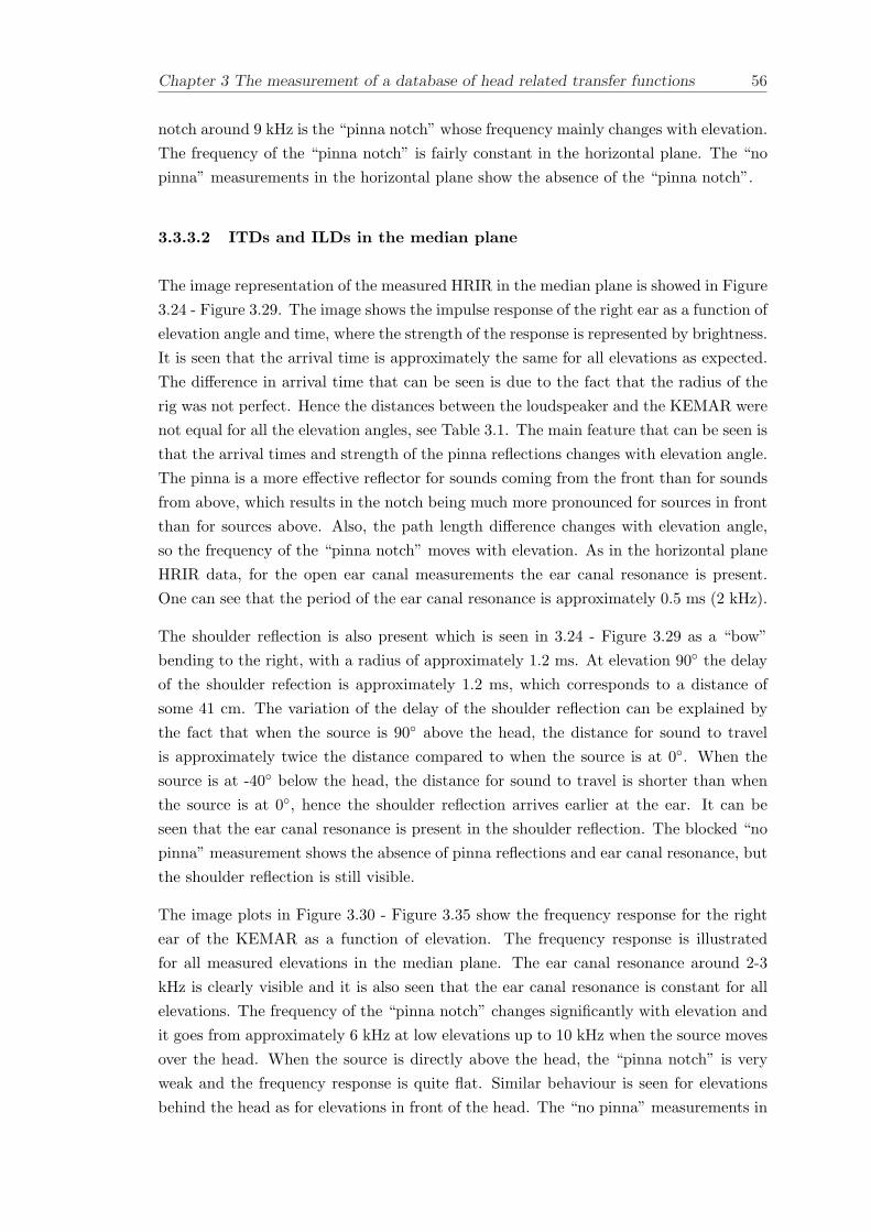
Chapter 3 The measurement of a database of head related transfer functions 56
notch around 9 kHz is the “pinna notch” whose frequency mainly changes with elevation.The frequency of the “pinna notch” is fairly constant in the horizontal plane. The “nopinna” measurements in the horizontal plane show the absence of the “pinna notch”.
3.3.3.2 ITDs and ILDs in the median plane
The image representation of the measured HRIR in the median plane is showed in Figure3.24 - Figure 3.29. The image shows the impulse response of the right ear as a function ofelevation angle and time, where the strength of the response is represented by brightness.It is seen that the arrival time is approximately the same for all elevations as expected.The difference in arrival time that can be seen is due to the fact that the radius of therig was not perfect. Hence the distances between the loudspeaker and the KEMAR werenot equal for all the elevation angles, see Table 3.1. The main feature that can be seen isthat the arrival times and strength of the pinna reflections changes with elevation angle.The pinna is a more effective reflector for sounds coming from the front than for soundsfrom above, which results in the notch being much more pronounced for sources in frontthan for sources above. Also, the path length difference changes with elevation angle,so the frequency of the “pinna notch” moves with elevation. As in the horizontal planeHRIR data, for the open ear canal measurements the ear canal resonance is present.One can see that the period of the ear canal resonance is approximately 0.5 ms (2 kHz).
The shoulder reflection is also present which is seen in 3.24 - Figure 3.29 as a “bow”bending to the right, with a radius of approximately 1.2 ms. At elevation 90 the delayof the shoulder refection is approximately 1.2 ms, which corresponds to a distance ofsome 41 cm. The variation of the delay of the shoulder reflection can be explained bythe fact that when the source is 90 above the head, the distance for sound to travelis approximately twice the distance compared to when the source is at 0. When thesource is at -40 below the head, the distance for sound to travel is shorter than whenthe source is at 0, hence the shoulder reflection arrives earlier at the ear. It can beseen that the ear canal resonance is present in the shoulder reflection. The blocked “nopinna” measurement shows the absence of pinna reflections and ear canal resonance, butthe shoulder reflection is still visible.
The image plots in Figure 3.30 - Figure 3.35 show the frequency response for the rightear of the KEMAR as a function of elevation. The frequency response is illustratedfor all measured elevations in the median plane. The ear canal resonance around 2-3kHz is clearly visible and it is also seen that the ear canal resonance is constant for allelevations. The frequency of the “pinna notch” changes significantly with elevation andit goes from approximately 6 kHz at low elevations up to 10 kHz when the source movesover the head. When the source is directly above the head, the “pinna notch” is veryweak and the frequency response is quite flat. Similar behaviour is seen for elevationsbehind the head as for elevations in front of the head. The “no pinna” measurements in
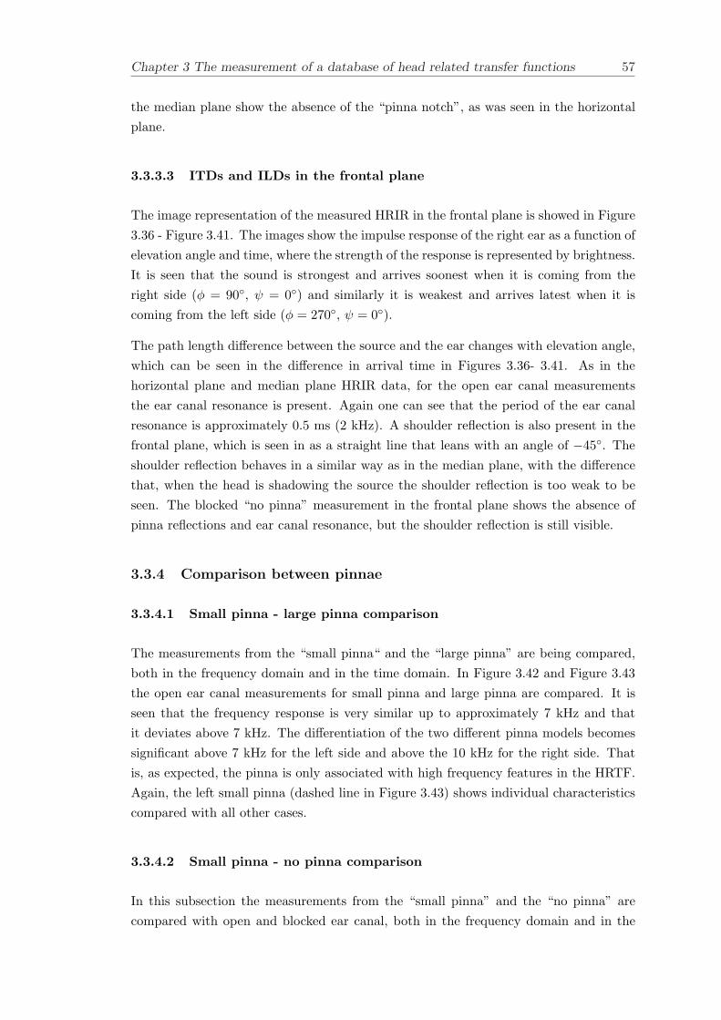
Chapter 3 The measurement of a database of head related transfer functions 57
the median plane show the absence of the “pinna notch”, as was seen in the horizontalplane.
3.3.3.3 ITDs and ILDs in the frontal plane
The image representation of the measured HRIR in the frontal plane is showed in Figure3.36 - Figure 3.41. The images show the impulse response of the right ear as a function ofelevation angle and time, where the strength of the response is represented by brightness.It is seen that the sound is strongest and arrives soonest when it is coming from theright side (φ = 90, ψ = 0) and similarly it is weakest and arrives latest when it iscoming from the left side (φ = 270, ψ = 0).
The path length difference between the source and the ear changes with elevation angle,which can be seen in the difference in arrival time in Figures 3.36- 3.41. As in thehorizontal plane and median plane HRIR data, for the open ear canal measurementsthe ear canal resonance is present. Again one can see that the period of the ear canalresonance is approximately 0.5 ms (2 kHz). A shoulder reflection is also present in thefrontal plane, which is seen in as a straight line that leans with an angle of −45. Theshoulder reflection behaves in a similar way as in the median plane, with the differencethat, when the head is shadowing the source the shoulder reflection is too weak to beseen. The blocked “no pinna” measurement in the frontal plane shows the absence ofpinna reflections and ear canal resonance, but the shoulder reflection is still visible.
3.3.4 Comparison between pinnae
3.3.4.1 Small pinna - large pinna comparison
The measurements from the “small pinna“ and the “large pinna” are being compared,both in the frequency domain and in the time domain. In Figure 3.42 and Figure 3.43the open ear canal measurements for small pinna and large pinna are compared. It isseen that the frequency response is very similar up to approximately 7 kHz and thatit deviates above 7 kHz. The differentiation of the two different pinna models becomessignificant above 7 kHz for the left side and above the 10 kHz for the right side. Thatis, as expected, the pinna is only associated with high frequency features in the HRTF.Again, the left small pinna (dashed line in Figure 3.43) shows individual characteristicscompared with all other cases.
3.3.4.2 Small pinna - no pinna comparison
In this subsection the measurements from the “small pinna” and the “no pinna” arecompared with open and blocked ear canal, both in the frequency domain and in the
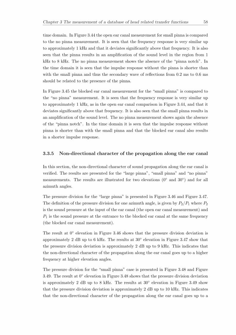
Chapter 3 The measurement of a database of head related transfer functions 58
time domain. In Figure 3.44 the open ear canal measurement for small pinna is comparedto the no pinna measurement. It is seen that the frequency response is very similar upto approximately 1 kHz and that it deviates significantly above that frequency. It is alsoseen that the pinna results in an amplification of the sound level in the region from 1kHz to 8 kHz. The no pinna measurement shows the absence of the “pinna notch”. Inthe time domain it is seen that the impulse response without the pinna is shorter thanwith the small pinna and thus the secondary wave of reflections from 0.2 ms to 0.6 msshould be related to the presence of the pinna.
In Figure 3.45 the blocked ear canal measurement for the “small pinna” is compared tothe “no pinna” measurement. It is seen that the frequency response is very similar upto approximately 1 kHz, as in the open ear canal comparison in Figure 3.44, and that itdeviates significantly above that frequency. It is also seen that the small pinna results inan amplification of the sound level. The no pinna measurement shows again the absenceof the “pinna notch”. In the time domain it is seen that the impulse response withoutpinna is shorter than with the small pinna and that the blocked ear canal also resultsin a shorter impulse response.
3.3.5 Non-directional character of the propagation along the ear canal
In this section, the non-directional character of sound propagation along the ear canal isverified. The results are presented for the “large pinna”, “small pinna” and “no pinna”measurements. The results are illustrated for two elevations (0 and 30) and for allazimuth angles.
The pressure division for the “large pinna” is presented in Figure 3.46 and Figure 3.47.The definition of the pressure division for one azimuth angle, is given by P2/P1 where P2
is the sound pressure at the input of the ear canal (the open ear canal measurement) andP1 is the sound pressure at the entrance to the blocked ear canal at the same frequency(the blocked ear canal measurement).
The result at 0 elevation in Figure 3.46 shows that the pressure division deviation isapproximately 2 dB up to 6 kHz. The results at 30 elevation in Figure 3.47 show thatthe pressure division deviation is approximately 2 dB up to 9 kHz. This indicates thatthe non-directional character of the propagation along the ear canal goes up to a higherfrequency at higher elevation angles.
The pressure division for the “small pinna” case is presented in Figure 3.48 and Figure3.49. The result at 0 elevation in Figure 3.48 shows that the pressure division deviationis approximately 2 dB up to 8 kHz. The results at 30 elevation in Figure 3.49 showthat the pressure division deviation is approximately 2 dB up to 10 kHz. This indicatesthat the non-directional character of the propagation along the ear canal goes up to a
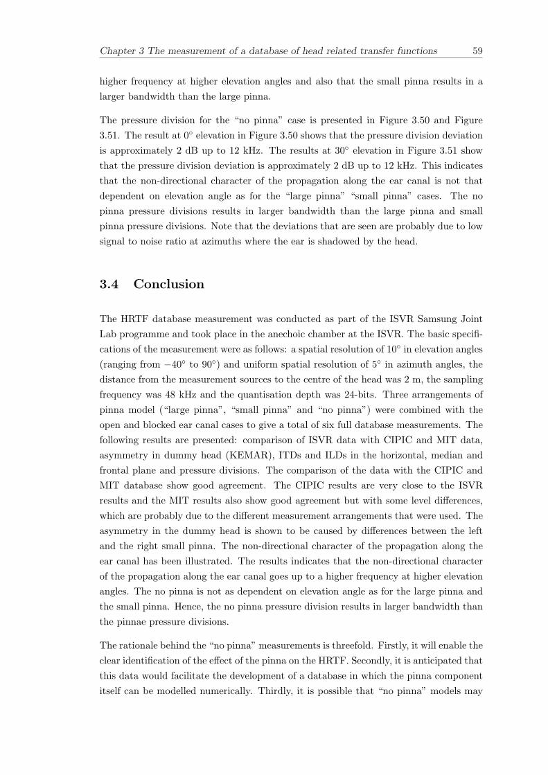
Chapter 3 The measurement of a database of head related transfer functions 59
higher frequency at higher elevation angles and also that the small pinna results in alarger bandwidth than the large pinna.
The pressure division for the “no pinna” case is presented in Figure 3.50 and Figure3.51. The result at 0 elevation in Figure 3.50 shows that the pressure division deviationis approximately 2 dB up to 12 kHz. The results at 30 elevation in Figure 3.51 showthat the pressure division deviation is approximately 2 dB up to 12 kHz. This indicatesthat the non-directional character of the propagation along the ear canal is not thatdependent on elevation angle as for the “large pinna” “small pinna” cases. The nopinna pressure divisions results in larger bandwidth than the large pinna and smallpinna pressure divisions. Note that the deviations that are seen are probably due to lowsignal to noise ratio at azimuths where the ear is shadowed by the head.
3.4 Conclusion
The HRTF database measurement was conducted as part of the ISVR Samsung JointLab programme and took place in the anechoic chamber at the ISVR. The basic specifi-cations of the measurement were as follows: a spatial resolution of 10 in elevation angles(ranging from −40 to 90) and uniform spatial resolution of 5 in azimuth angles, thedistance from the measurement sources to the centre of the head was 2 m, the samplingfrequency was 48 kHz and the quantisation depth was 24-bits. Three arrangements ofpinna model (“large pinna”, “small pinna” and “no pinna”) were combined with theopen and blocked ear canal cases to give a total of six full database measurements. Thefollowing results are presented: comparison of ISVR data with CIPIC and MIT data,asymmetry in dummy head (KEMAR), ITDs and ILDs in the horizontal, median andfrontal plane and pressure divisions. The comparison of the data with the CIPIC andMIT database show good agreement. The CIPIC results are very close to the ISVRresults and the MIT results also show good agreement but with some level differences,which are probably due to the different measurement arrangements that were used. Theasymmetry in the dummy head is shown to be caused by differences between the leftand the right small pinna. The non-directional character of the propagation along theear canal has been illustrated. The results indicates that the non-directional characterof the propagation along the ear canal goes up to a higher frequency at higher elevationangles. The no pinna is not as dependent on elevation angle as for the large pinna andthe small pinna. Hence, the no pinna pressure division results in larger bandwidth thanthe pinnae pressure divisions.
The rationale behind the “no pinna” measurements is threefold. Firstly, it will enable theclear identification of the effect of the pinna on the HRTF. Secondly, it is anticipated thatthis data would facilitate the development of a database in which the pinna componentitself can be modelled numerically. Thirdly, it is possible that “no pinna” models may

Chapter 3 The measurement of a database of head related transfer functions 60
be useful in the design of virtual sound imaging systems. This use, however, may varybetween loudspeaker and headphone based systems. To conclude, the outcome of thismeasurement have resulted in the most extensive HRTF KEMAR database yet available.The data that has been collected show good agreement with other databases, such asthe CIPIC and the MIT database. The combination of the six different measurementcases aims to be a starting point for future modelling of pinna responses. The databasehas been used for the objective evaluation of interpolation techniques in the followingchapter and for the simulations of cross-talk cancellation effectiveness in Chapter 5
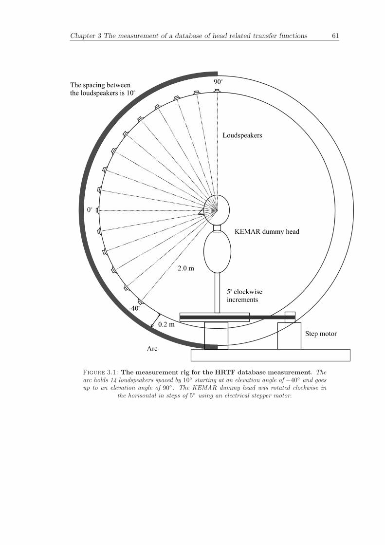
Chapter 3 The measurement of a database of head related transfer functions 61
2.0 m
0.2 m
The spacing betweenthe loudspeakers is 10
o
90o
0o
-40o
Step motor
5 clockwiseincrements
o
KEMAR dummy head
Arc
Loudspeakers
Figure 3.1: The measurement rig for the HRTF database measurement. Thearc holds 14 loudspeakers spaced by 10 starting at an elevation angle of −40 and goesup to an elevation angle of 90. The KEMAR dummy head was rotated clockwise in
the horisontal in steps of 5 using an electrical stepper motor.
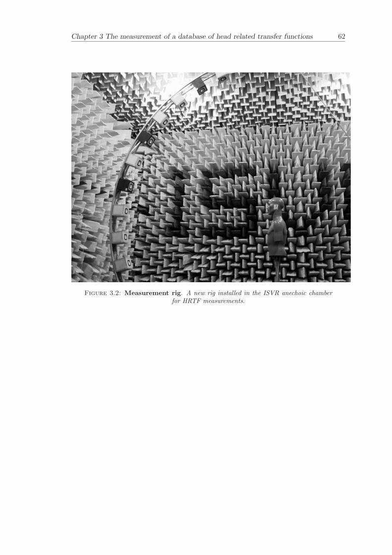
Chapter 3 The measurement of a database of head related transfer functions 62
Figure 3.2: Measurement rig. A new rig installed in the ISVR anechoic chamberfor HRTF measurements.
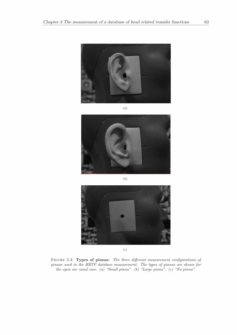
Chapter 3 The measurement of a database of head related transfer functions 63
(a)
(b)
(c)
Figure 3.3: Types of pinnae. The three different measurement configurations ofpinnae used in the HRTF database measurement. The types of pinnae are shown for
the open ear canal case. (a) “Small pinna”. (b) “Large pinna”. (c) “No pinna”.
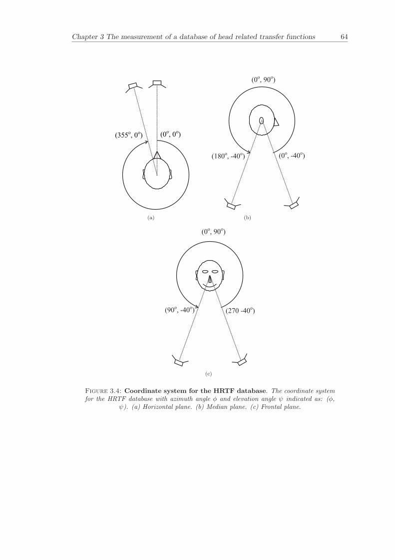
Chapter 3 The measurement of a database of head related transfer functions 64
(355o, 0
o) (0
o, 0
o)
(a)
(0o, 90
o)
(180o, -40
o) (0
o, -40
o)
(b)
(0o, 90
o)
(270 -40o)
(c)
Figure 3.4: Coordinate system for the HRTF database. The coordinate systemfor the HRTF database with azimuth angle φ and elevation angle ψ indicated as: (φ,
ψ). (a) Horizontal plane. (b) Median plane. (c) Frontal plane.
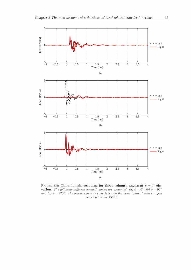
Chapter 3 The measurement of a database of head related transfer functions 65
−1 −0.5 0 0.5 1 1.5 2 2.5 3 3.5 4−5
0
5
Time [ms]
Leve
l [P
a/P
a]LeftRight
(a)
−1 −0.5 0 0.5 1 1.5 2 2.5 3 3.5 4−5
0
5
Time [ms]
Leve
l [P
a/P
a]
LeftRight
(b)
−1 −0.5 0 0.5 1 1.5 2 2.5 3 3.5 4−5
0
5
Time [ms]
Leve
l [P
a/P
a]
LeftRight
(c)
Figure 3.5: Time domain response for three azimuth angles at ψ = 0 ele-vation. The following different azimuth angles are presented: (a) φ = 0, (b) φ = 90
and (c) φ = 270. The measurement is undertaken on the “small pinna” with an openear canal at the ISVR.
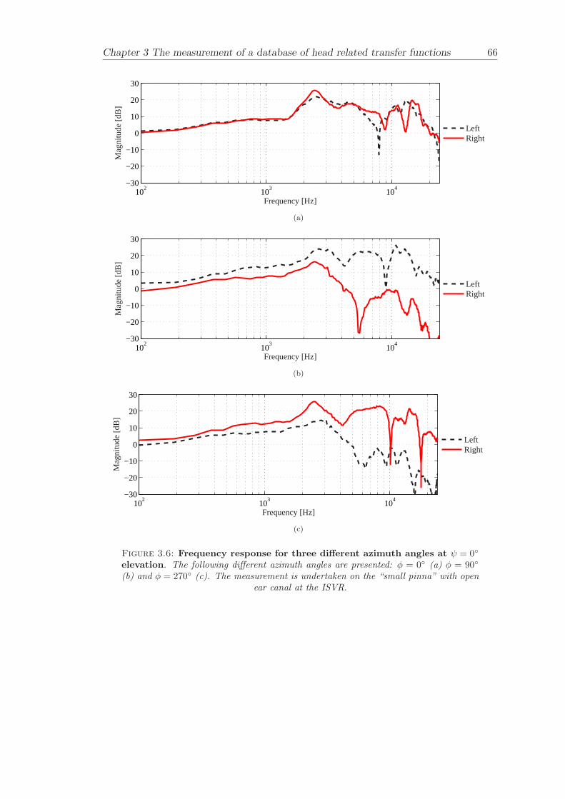
Chapter 3 The measurement of a database of head related transfer functions 66
102
103
104
−30
−20
−10
0
10
20
30
Frequency [Hz]
Mag
nitu
de [d
B]
LeftRight
(a)
102
103
104
−30
−20
−10
0
10
20
30
Frequency [Hz]
Mag
nitu
de [d
B]
LeftRight
(b)
102
103
104
−30
−20
−10
0
10
20
30
Frequency [Hz]
Mag
nitu
de [d
B]
LeftRight
(c)
Figure 3.6: Frequency response for three different azimuth angles at ψ = 0
elevation. The following different azimuth angles are presented: φ = 0 (a) φ = 90
(b) and φ = 270 (c). The measurement is undertaken on the “small pinna” with openear canal at the ISVR.
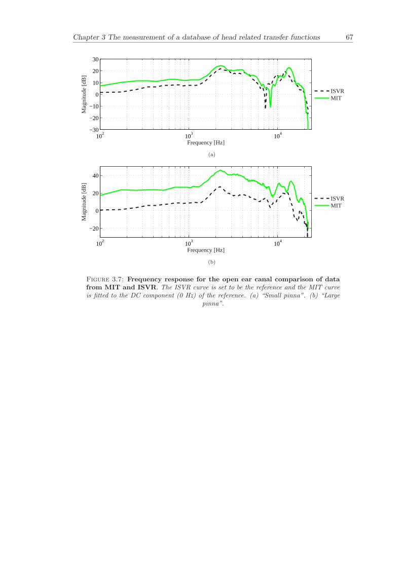
Chapter 3 The measurement of a database of head related transfer functions 67
102
103
104
−30
−20
−10
0
10
20
30
Frequency [Hz]
Mag
nitu
de [d
B]
ISVRMIT
(a)
102
103
104
−20
0
20
40
Frequency [Hz]
Mag
nitu
de [d
B]
ISVRMIT
(b)
Figure 3.7: Frequency response for the open ear canal comparison of datafrom MIT and ISVR. The ISVR curve is set to be the reference and the MIT curveis fitted to the DC component (0 Hz) of the reference. (a) “Small pinna”. (b) “Large
pinna”.
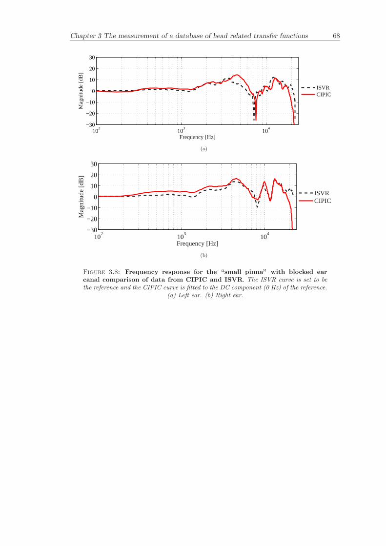
Chapter 3 The measurement of a database of head related transfer functions 68
102
103
104
−30
−20
−10
0
10
20
30
Frequency [Hz]
Mag
nitu
de [d
B]
ISVRCIPIC
(a)
102
103
104
−30
−20
−10
0
10
20
30
Frequency [Hz]
Mag
nitu
de [d
B]
ISVRCIPIC
(b)
Figure 3.8: Frequency response for the “small pinna” with blocked earcanal comparison of data from CIPIC and ISVR. The ISVR curve is set to bethe reference and the CIPIC curve is fitted to the DC component (0 Hz) of the reference.
(a) Left ear. (b) Right ear.
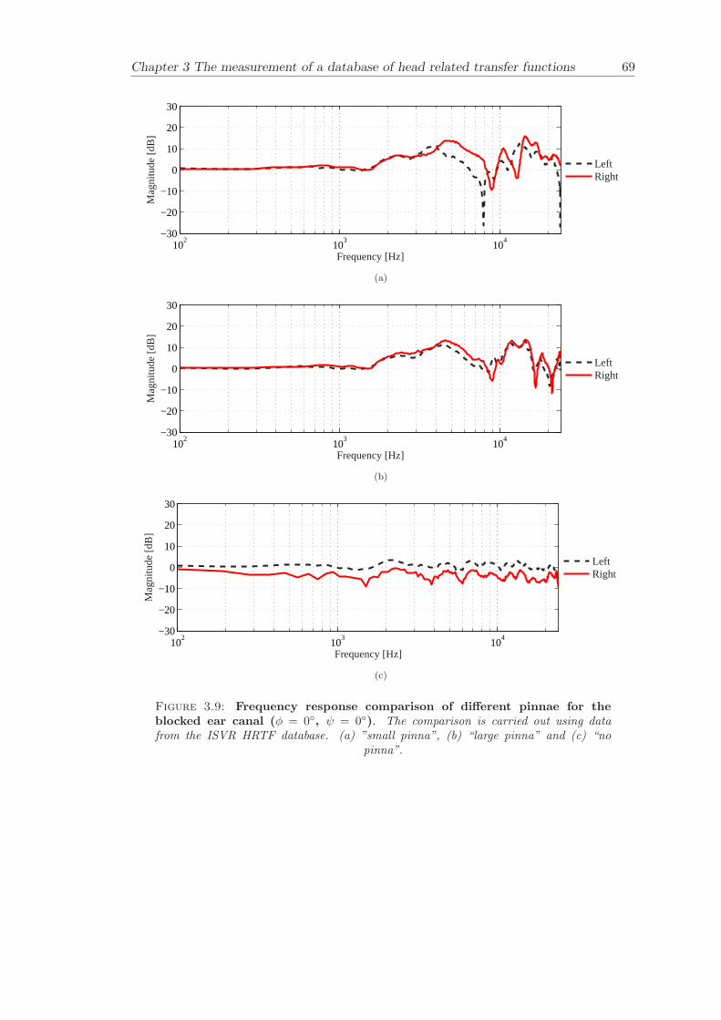
Chapter 3 The measurement of a database of head related transfer functions 69
102
103
104
−30
−20
−10
0
10
20
30
Frequency [Hz]
Mag
nitu
de [d
B]
LeftRight
(a)
102
103
104
−30
−20
−10
0
10
20
30
Frequency [Hz]
Mag
nitu
de [d
B]
LeftRight
(b)
102
103
104
−30
−20
−10
0
10
20
30
Frequency [Hz]
Mag
nitu
de [d
B]
LeftRight
(c)
Figure 3.9: Frequency response comparison of different pinnae for theblocked ear canal (φ = 0, ψ = 0). The comparison is carried out using datafrom the ISVR HRTF database. (a) ”small pinna”, (b) “large pinna” and (c) “no
pinna”.
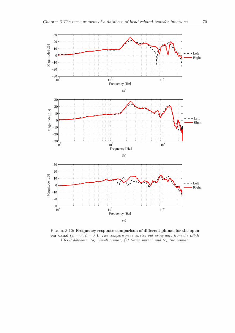
Chapter 3 The measurement of a database of head related transfer functions 70
102
103
104
−30
−20
−10
0
10
20
30
Frequency [Hz]
Mag
nitu
de [d
B]
LeftRight
(a)
102
103
104
−30
−20
−10
0
10
20
30
Frequency [Hz]
Mag
nitu
de [d
B]
LeftRight
(b)
102
103
104
−30
−20
−10
0
10
20
30
Frequency [Hz]
Mag
nitu
de [d
B]
LeftRight
(c)
Figure 3.10: Frequency response comparison of different pinnae for the openear canal (φ = 0,ψ = 0). The comparison is carried out using data from the ISVR
HRTF database. (a) “small pinna”, (b) “large pinna” and (c) “no pinna”.
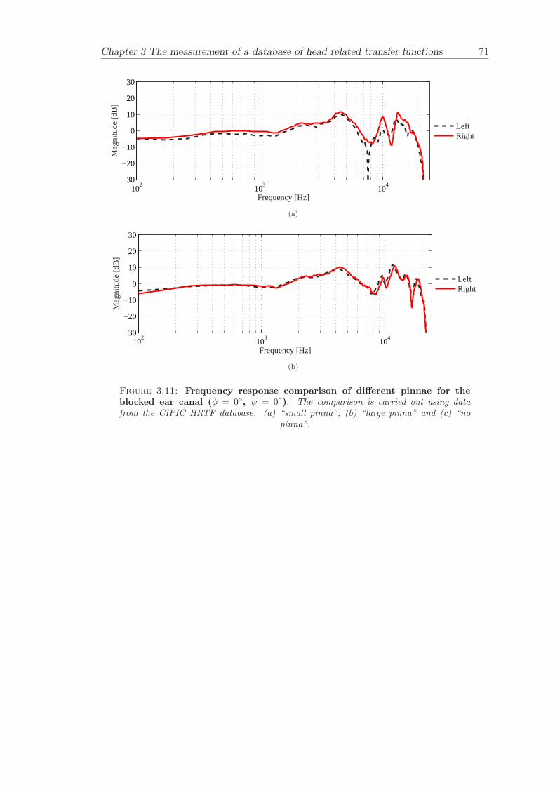
Chapter 3 The measurement of a database of head related transfer functions 71
102
103
104
−30
−20
−10
0
10
20
30
Frequency [Hz]
Mag
nitu
de [d
B]
LeftRight
(a)
102
103
104
−30
−20
−10
0
10
20
30
Frequency [Hz]
Mag
nitu
de [d
B]
LeftRight
(b)
Figure 3.11: Frequency response comparison of different pinnae for theblocked ear canal (φ = 0, ψ = 0). The comparison is carried out using datafrom the CIPIC HRTF database. (a) “small pinna”, (b) “large pinna” and (c) “no
pinna”.

Chapter 3 The measurement of a database of head related transfer functions 72
Tim
e [m
s]
Azimuth angle [°]
[Pa/Pa]
0 50 100 150 200 250 300 350
−1
−0.5
0
0.5
1
1.5
2−2
−1.5
−1
−0.5
0
0.5
1
1.5
2
Figure 3.12: HRIR in the horizontal plane for the right open ear canal“small pinna”. The time domain response is plotted as a function of azimuth angle
φ.
Tim
e [m
s]
Azimuth angle [°]
[Pa/Pa]
0 50 100 150 200 250 300 350
−1
−0.5
0
0.5
1
1.5
2−2
−1.5
−1
−0.5
0
0.5
1
1.5
2
Figure 3.13: HRIR in the horizontal plane for the right open ear canal“large pinna”. The time domain response is plotted as a function of azimuth angle φ.

Chapter 3 The measurement of a database of head related transfer functions 73
Tim
e [m
s]
Azimuth angle [°]
[Pa/Pa]
0 50 100 150 200 250 300 350
−1
−0.5
0
0.5
1
1.5
2−2
−1.5
−1
−0.5
0
0.5
1
1.5
2
Figure 3.14: HRIR in the horizontal plane for the right open ear canal “nopinna”. The time domain response is plotted as a function of azimuth angle φ.
Tim
e [m
s]
Azimuth angle [°]
[Pa/Pa]
0 50 100 150 200 250 300 350
−1
−0.5
0
0.5
1
1.5
2−2
−1.5
−1
−0.5
0
0.5
1
1.5
2
Figure 3.15: HRIR in the horizontal plane for the right blocked ear canal“small pinna”. The time domain response is plotted as a function of azimuth angle
φ.
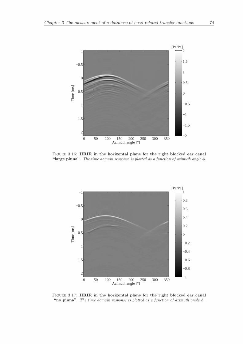
Chapter 3 The measurement of a database of head related transfer functions 74
Tim
e [m
s]
Azimuth angle [°]
[Pa/Pa]
0 50 100 150 200 250 300 350
−1
−0.5
0
0.5
1
1.5
2−2
−1.5
−1
−0.5
0
0.5
1
1.5
2
Figure 3.16: HRIR in the horizontal plane for the right blocked ear canal“large pinna”. The time domain response is plotted as a function of azimuth angle φ.
Tim
e [m
s]
Azimuth angle [°]
[Pa/Pa]
0 50 100 150 200 250 300 350
−1
−0.5
0
0.5
1
1.5
2−1
−0.8
−0.6
−0.4
−0.2
0
0.2
0.4
0.6
0.8
1
Figure 3.17: HRIR in the horizontal plane for the right blocked ear canal“no pinna”. The time domain response is plotted as a function of azimuth angle φ.
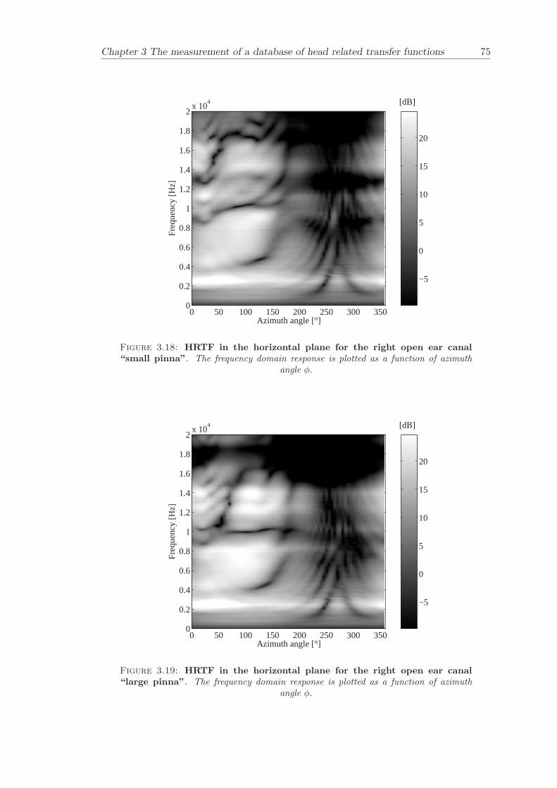
Chapter 3 The measurement of a database of head related transfer functions 75
Azimuth angle [°]
Fre
quen
cy [H
z]
[dB]
0 50 100 150 200 250 300 3500
0.2
0.4
0.6
0.8
1
1.2
1.4
1.6
1.8
2x 10
4
−5
0
5
10
15
20
Figure 3.18: HRTF in the horizontal plane for the right open ear canal“small pinna”. The frequency domain response is plotted as a function of azimuth
angle φ.
Azimuth angle [°]
Fre
quen
cy [H
z]
[dB]
0 50 100 150 200 250 300 3500
0.2
0.4
0.6
0.8
1
1.2
1.4
1.6
1.8
2x 10
4
−5
0
5
10
15
20
Figure 3.19: HRTF in the horizontal plane for the right open ear canal“large pinna”. The frequency domain response is plotted as a function of azimuth
angle φ.
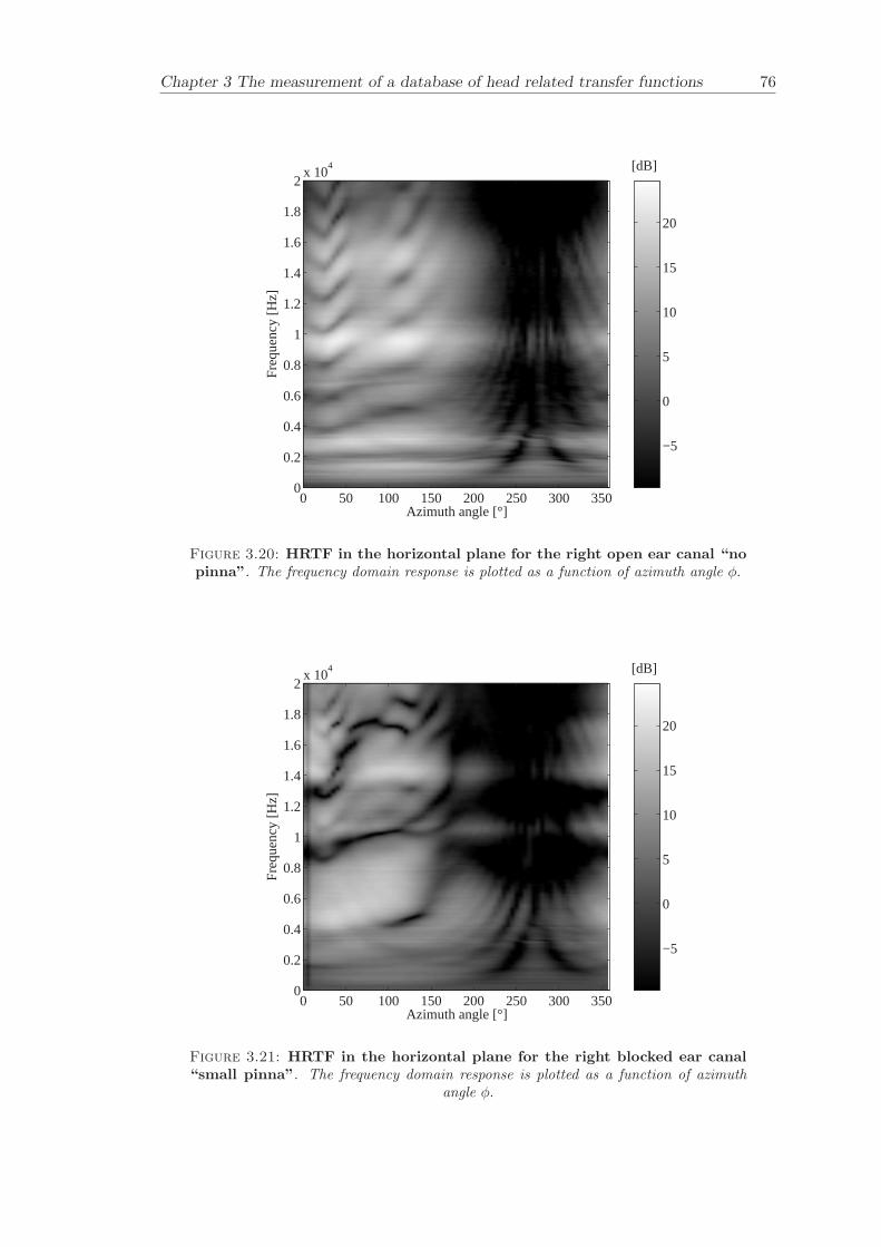
Chapter 3 The measurement of a database of head related transfer functions 76
Azimuth angle [°]
Fre
quen
cy [H
z]
[dB]
0 50 100 150 200 250 300 3500
0.2
0.4
0.6
0.8
1
1.2
1.4
1.6
1.8
2x 10
4
−5
0
5
10
15
20
Figure 3.20: HRTF in the horizontal plane for the right open ear canal “nopinna”. The frequency domain response is plotted as a function of azimuth angle φ.
Azimuth angle [°]
Fre
quen
cy [H
z]
[dB]
0 50 100 150 200 250 300 3500
0.2
0.4
0.6
0.8
1
1.2
1.4
1.6
1.8
2x 10
4
−5
0
5
10
15
20
Figure 3.21: HRTF in the horizontal plane for the right blocked ear canal“small pinna”. The frequency domain response is plotted as a function of azimuth
angle φ.
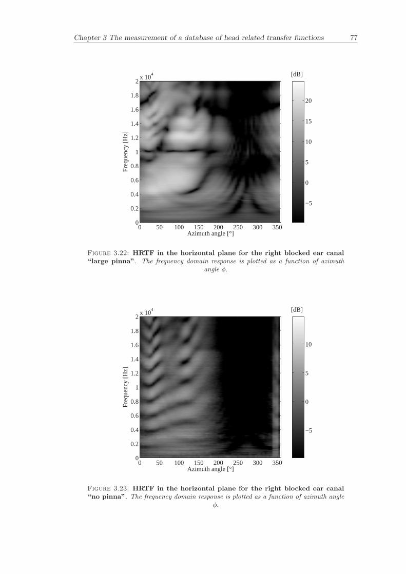
Chapter 3 The measurement of a database of head related transfer functions 77
Azimuth angle [°]
Fre
quen
cy [H
z]
[dB]
0 50 100 150 200 250 300 3500
0.2
0.4
0.6
0.8
1
1.2
1.4
1.6
1.8
2x 10
4
−5
0
5
10
15
20
Figure 3.22: HRTF in the horizontal plane for the right blocked ear canal“large pinna”. The frequency domain response is plotted as a function of azimuth
angle φ.
Azimuth angle [°]
Fre
quen
cy [H
z]
[dB]
0 50 100 150 200 250 300 3500
0.2
0.4
0.6
0.8
1
1.2
1.4
1.6
1.8
2x 10
4
−5
0
5
10
Figure 3.23: HRTF in the horizontal plane for the right blocked ear canal“no pinna”. The frequency domain response is plotted as a function of azimuth angle
φ.

Chapter 3 The measurement of a database of head related transfer functions 78
Tim
e [m
s]
Elevation angle [°]
[Pa/Pa]
90° Az. 270° Az.
−40 0 40 90 40 0 −40
−1
−0.5
0
0.5
1
1.5
2−2
−1.5
−1
−0.5
0
0.5
1
1.5
2
Figure 3.24: HRIR in the median plane for the right open ear canal with“small pinna”. The time domain response is plotted as a function of elevation angle
ψ.
Tim
e [m
s]
Elevation angle [°]
[Pa/Pa]
90° Az. 270° Az.
−40 0 40 90 40 0 −40
−1
−0.5
0
0.5
1
1.5
2−2
−1.5
−1
−0.5
0
0.5
1
1.5
2
Figure 3.25: HRIR in the median plane for the right open ear canal with“large pinna”. The time domain response is plotted as a function of elevation angle
ψ.
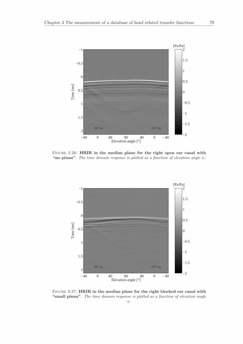
Chapter 3 The measurement of a database of head related transfer functions 79
Tim
e [m
s]
Elevation angle [°]
[Pa/Pa]
90° Az. 270° Az.
−40 0 40 90 40 0 −40
−1
−0.5
0
0.5
1
1.5
2−2
−1.5
−1
−0.5
0
0.5
1
1.5
2
Figure 3.26: HRIR in the median plane for the right open ear canal with“no pinna”. The time domain response is plotted as a function of elevation angle ψ.
Tim
e [m
s]
Elevation angle [°]
[Pa/Pa]
90° Az. 270° Az.
−40 0 40 90 40 0 −40
−1
−0.5
0
0.5
1
1.5
2−2
−1.5
−1
−0.5
0
0.5
1
1.5
2
Figure 3.27: HRIR in the median plane for the right blocked ear canal with“small pinna”. The time domain response is plotted as a function of elevation angle
ψ.
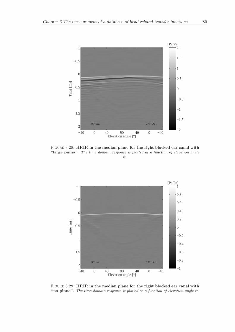
Chapter 3 The measurement of a database of head related transfer functions 80
Tim
e [m
s]
Elevation angle [°]
[Pa/Pa]
90° Az. 270° Az.
−40 0 40 90 40 0 −40
−1
−0.5
0
0.5
1
1.5
2−2
−1.5
−1
−0.5
0
0.5
1
1.5
2
Figure 3.28: HRIR in the median plane for the right blocked ear canal with“large pinna”. The time domain response is plotted as a function of elevation angle
ψ.
Tim
e [m
s]
Elevation angle [°]
[Pa/Pa]
90° Az. 270° Az.
−40 0 40 90 40 0 −40
−1
−0.5
0
0.5
1
1.5
2−1
−0.8
−0.6
−0.4
−0.2
0
0.2
0.4
0.6
0.8
1
Figure 3.29: HRIR in the median plane for the right blocked ear canal with“no pinna”. The time domain response is plotted as a function of elevation angle ψ.
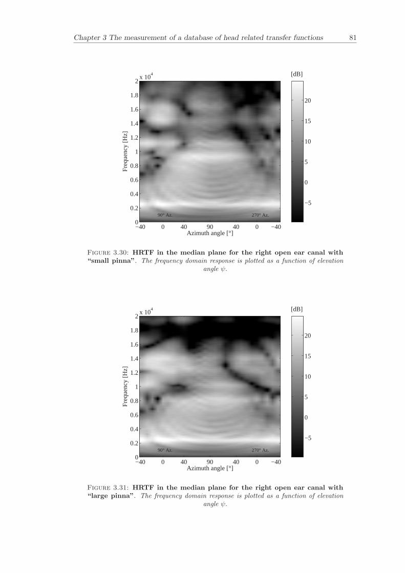
Chapter 3 The measurement of a database of head related transfer functions 81
Azimuth angle [°]
Fre
quen
cy [H
z]
[dB]
90° Az. 270° Az.
−40 0 40 90 40 0 −400
0.2
0.4
0.6
0.8
1
1.2
1.4
1.6
1.8
2x 10
4
−5
0
5
10
15
20
Figure 3.30: HRTF in the median plane for the right open ear canal with“small pinna”. The frequency domain response is plotted as a function of elevation
angle ψ.
Azimuth angle [°]
Fre
quen
cy [H
z]
[dB]
90° Az. 270° Az.
−40 0 40 90 40 0 −400
0.2
0.4
0.6
0.8
1
1.2
1.4
1.6
1.8
2x 10
4
−5
0
5
10
15
20
Figure 3.31: HRTF in the median plane for the right open ear canal with“large pinna”. The frequency domain response is plotted as a function of elevation
angle ψ.
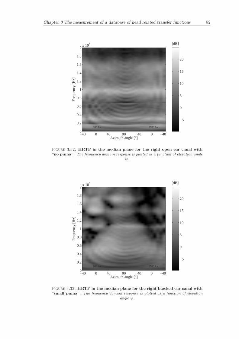
Chapter 3 The measurement of a database of head related transfer functions 82
Azimuth angle [°]
Fre
quen
cy [H
z]
[dB]
90° Az. 270° Az.
−40 0 40 90 40 0 −400
0.2
0.4
0.6
0.8
1
1.2
1.4
1.6
1.8
2x 10
4
−5
0
5
10
15
20
Figure 3.32: HRTF in the median plane for the right open ear canal with“no pinna”. The frequency domain response is plotted as a function of elevation angle
ψ.
Azimuth angle [°]
Fre
quen
cy [H
z]
[dB]
90° Az. 270° Az.
−40 0 40 90 40 0 −400
0.2
0.4
0.6
0.8
1
1.2
1.4
1.6
1.8
2x 10
4
−5
0
5
10
15
20
Figure 3.33: HRTF in the median plane for the right blocked ear canal with“small pinna”. The frequency domain response is plotted as a function of elevation
angle ψ.
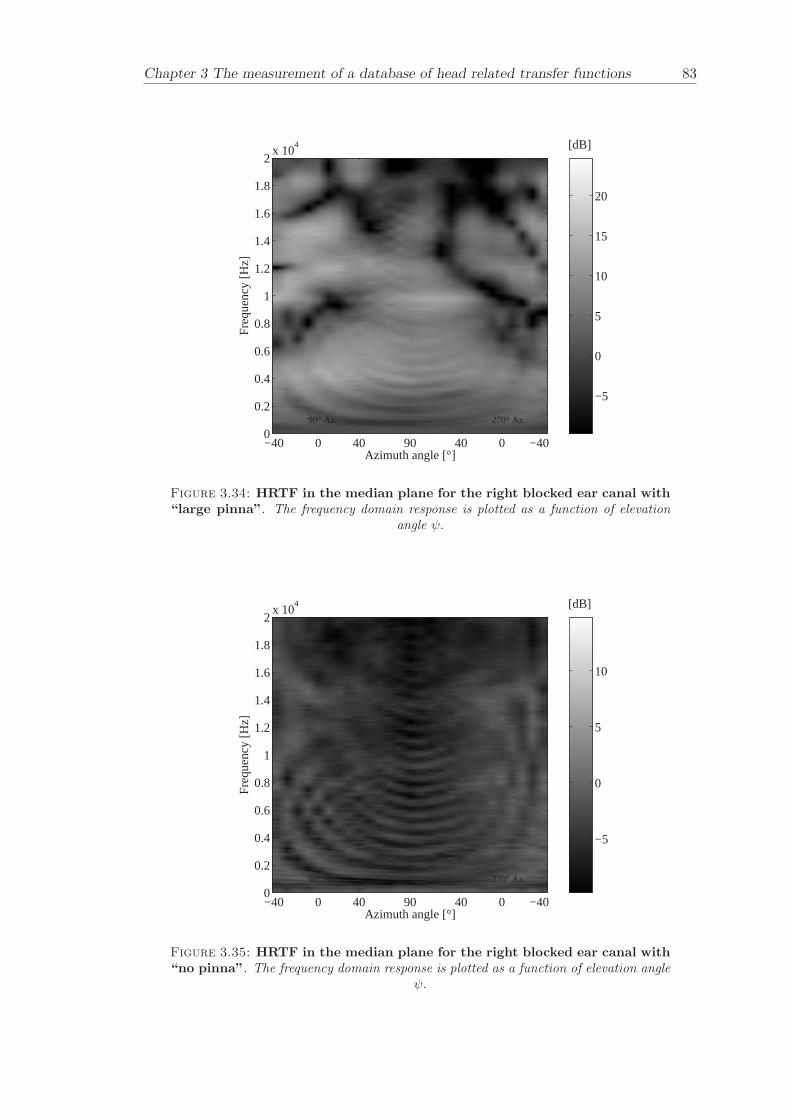
Chapter 3 The measurement of a database of head related transfer functions 83
Azimuth angle [°]
Fre
quen
cy [H
z]
[dB]
90° Az. 270° Az.
−40 0 40 90 40 0 −400
0.2
0.4
0.6
0.8
1
1.2
1.4
1.6
1.8
2x 10
4
−5
0
5
10
15
20
Figure 3.34: HRTF in the median plane for the right blocked ear canal with“large pinna”. The frequency domain response is plotted as a function of elevation
angle ψ.
Azimuth angle [°]
Fre
quen
cy [H
z]
[dB]
90° Az. 270° Az.
−40 0 40 90 40 0 −400
0.2
0.4
0.6
0.8
1
1.2
1.4
1.6
1.8
2x 10
4
−5
0
5
10
Figure 3.35: HRTF in the median plane for the right blocked ear canal with“no pinna”. The frequency domain response is plotted as a function of elevation angle
ψ.
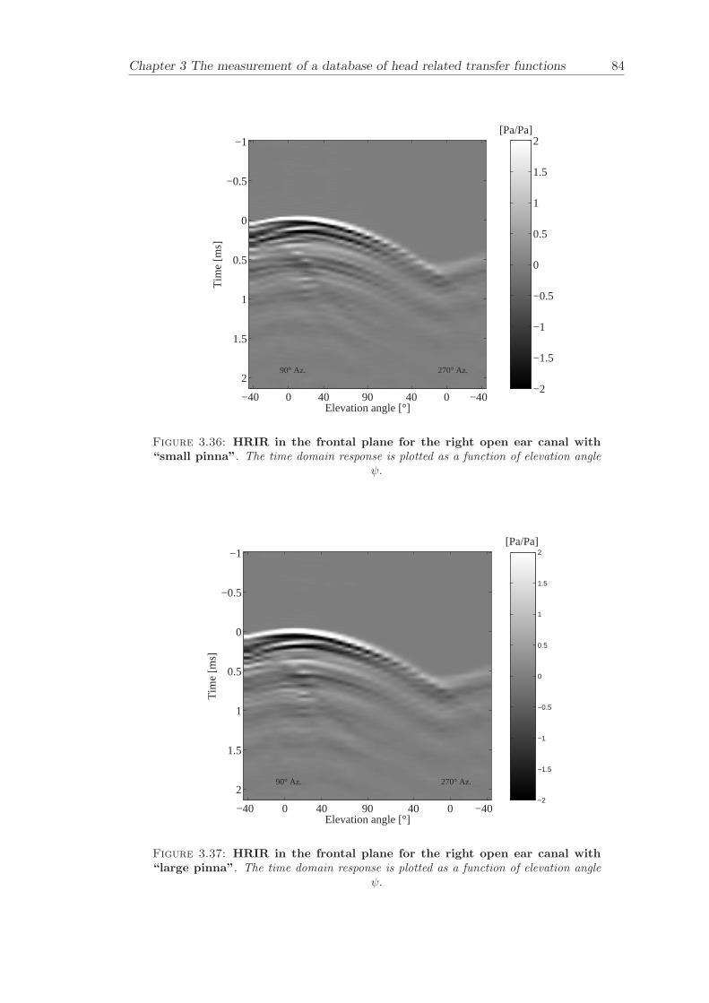
Chapter 3 The measurement of a database of head related transfer functions 84
Tim
e [m
s]
Elevation angle [°]
[Pa/Pa]
90° Az. 270° Az.
−40 0 40 90 40 0 −40
−1
−0.5
0
0.5
1
1.5
2−2
−1.5
−1
−0.5
0
0.5
1
1.5
2
Figure 3.36: HRIR in the frontal plane for the right open ear canal with“small pinna”. The time domain response is plotted as a function of elevation angle
ψ.
Tim
e [m
s]
Elevation angle [°]
[Pa/Pa]
90° Az. 270° Az.
−40 0 40 90 40 0 −40
−1
−0.5
0
0.5
1
1.5
2−2
−1.5
−1
−0.5
0
0.5
1
1.5
2
Figure 3.37: HRIR in the frontal plane for the right open ear canal with“large pinna”. The time domain response is plotted as a function of elevation angle
ψ.
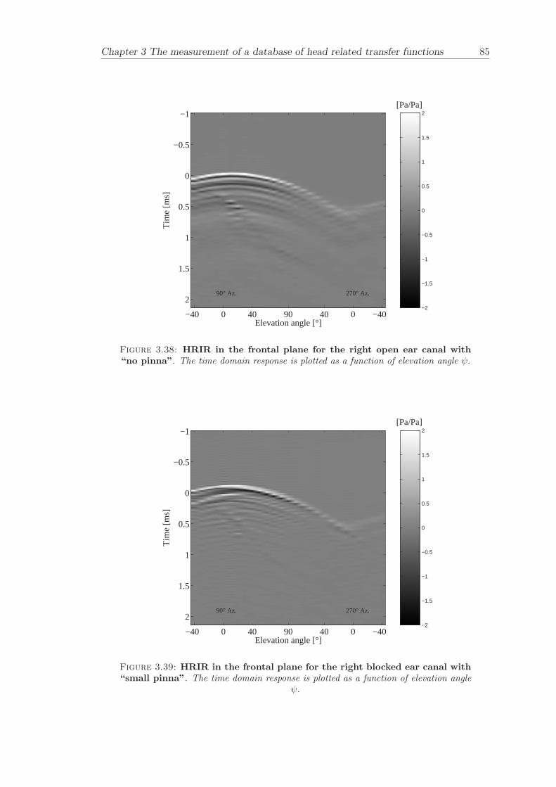
Chapter 3 The measurement of a database of head related transfer functions 85
Tim
e [m
s]
Elevation angle [°]
[Pa/Pa]
90° Az. 270° Az.
−40 0 40 90 40 0 −40
−1
−0.5
0
0.5
1
1.5
2−2
−1.5
−1
−0.5
0
0.5
1
1.5
2
Figure 3.38: HRIR in the frontal plane for the right open ear canal with“no pinna”. The time domain response is plotted as a function of elevation angle ψ.
Tim
e [m
s]
Elevation angle [°]
[Pa/Pa]
90° Az. 270° Az.
−40 0 40 90 40 0 −40
−1
−0.5
0
0.5
1
1.5
2−2
−1.5
−1
−0.5
0
0.5
1
1.5
2
Figure 3.39: HRIR in the frontal plane for the right blocked ear canal with“small pinna”. The time domain response is plotted as a function of elevation angle
ψ.
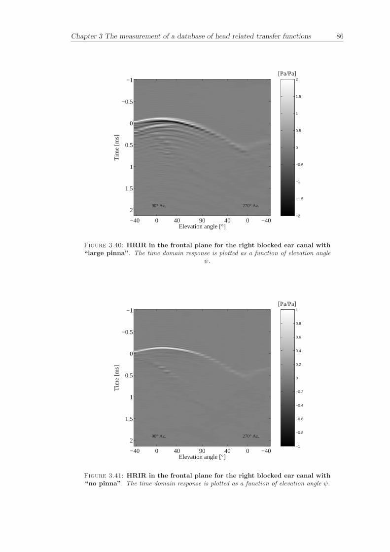
Chapter 3 The measurement of a database of head related transfer functions 86
Tim
e [m
s]
Elevation angle [°]
[Pa/Pa]
90° Az. 270° Az.
−40 0 40 90 40 0 −40
−1
−0.5
0
0.5
1
1.5
2−2
−1.5
−1
−0.5
0
0.5
1
1.5
2
Figure 3.40: HRIR in the frontal plane for the right blocked ear canal with“large pinna”. The time domain response is plotted as a function of elevation angle
ψ.
Tim
e [m
s]
Elevation angle [°]
[Pa/Pa]
90° Az. 270° Az.
−40 0 40 90 40 0 −40
−1
−0.5
0
0.5
1
1.5
2−1
−0.8
−0.6
−0.4
−0.2
0
0.2
0.4
0.6
0.8
1
Figure 3.41: HRIR in the frontal plane for the right blocked ear canal with“no pinna”. The time domain response is plotted as a function of elevation angle ψ.
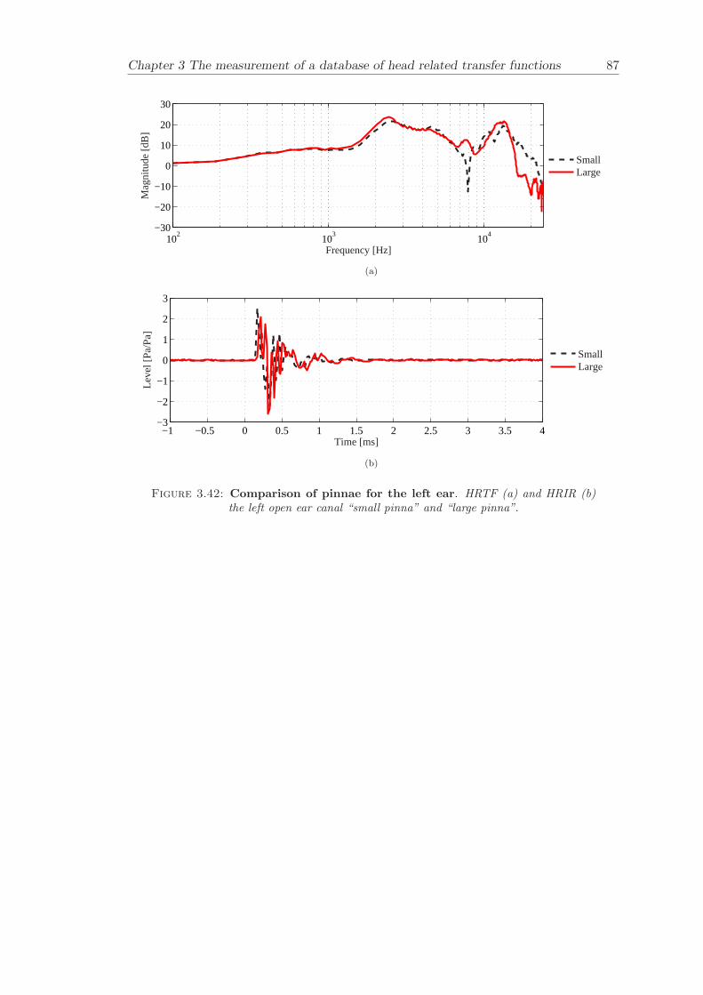
Chapter 3 The measurement of a database of head related transfer functions 87
102
103
104
−30
−20
−10
0
10
20
30
Frequency [Hz]
Mag
nitu
de [d
B]
SmallLarge
(a)
−1 −0.5 0 0.5 1 1.5 2 2.5 3 3.5 4−3
−2
−1
0
1
2
3
Time [ms]
Leve
l [P
a/P
a]
SmallLarge
(b)
Figure 3.42: Comparison of pinnae for the left ear. HRTF (a) and HRIR (b)the left open ear canal “small pinna” and “large pinna”.
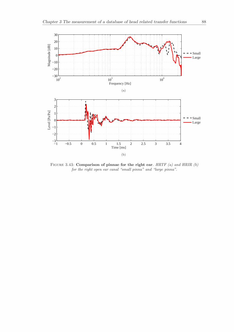
Chapter 3 The measurement of a database of head related transfer functions 88
102
103
104
−30
−20
−10
0
10
20
30
Frequency [Hz]
Mag
nitu
de [d
B]
SmallLarge
(a)
−1 −0.5 0 0.5 1 1.5 2 2.5 3 3.5 4−3
−2
−1
0
1
2
3
Time [ms]
Leve
l [P
a/P
a]
SmallLarge
(b)
Figure 3.43: Comparison of pinnae for the right ear. HRTF (a) and HRIR (b)for the right open ear canal “small pinna” and “large pinna”.
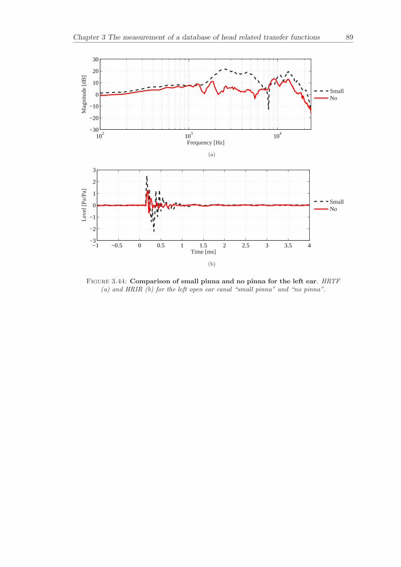
Chapter 3 The measurement of a database of head related transfer functions 89
102
103
104
−30
−20
−10
0
10
20
30
Frequency [Hz]
Mag
nitu
de [d
B]
SmallNo
(a)
−1 −0.5 0 0.5 1 1.5 2 2.5 3 3.5 4−3
−2
−1
0
1
2
3
Time [ms]
Leve
l [P
a/P
a]
SmallNo
(b)
Figure 3.44: Comparison of small pinna and no pinna for the left ear. HRTF(a) and HRIR (b) for the left open ear canal “small pinna” and “no pinna”.
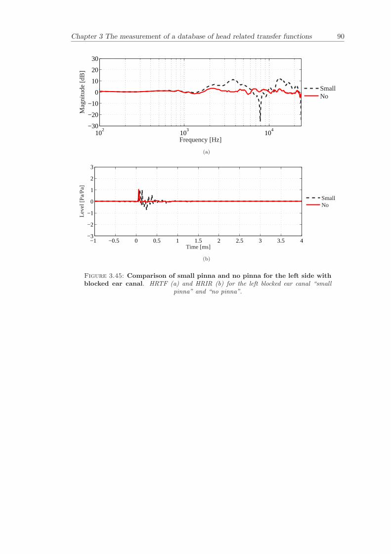
Chapter 3 The measurement of a database of head related transfer functions 90
102
103
104
−30
−20
−10
0
10
20
30
Frequency [Hz]
Mag
nitu
de [d
B]
SmallNo
(a)
−1 −0.5 0 0.5 1 1.5 2 2.5 3 3.5 4−3
−2
−1
0
1
2
3
Time [ms]
Leve
l [P
a/P
a]
SmallNo
(b)
Figure 3.45: Comparison of small pinna and no pinna for the left side withblocked ear canal. HRTF (a) and HRIR (b) for the left blocked ear canal “small
pinna” and “no pinna”.
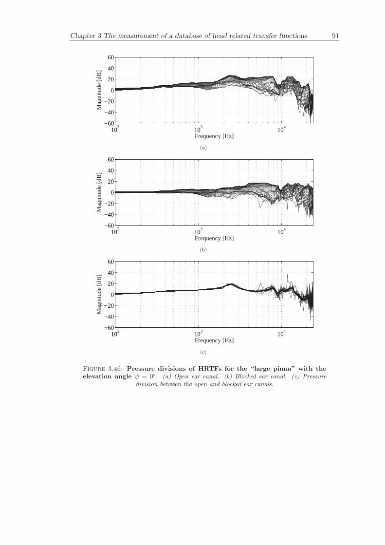
Chapter 3 The measurement of a database of head related transfer functions 91
102
103
104
−60
−40
−20
0
20
40
60
Frequency [Hz]
Mag
nitu
de [d
B]
(a)
102
103
104
−60
−40
−20
0
20
40
60
Frequency [Hz]
Mag
nitu
de [d
B]
(b)
102
103
104
−60
−40
−20
0
20
40
60
Frequency [Hz]
Mag
nitu
de [d
B]
(c)
Figure 3.46: Pressure divisions of HRTFs for the “large pinna” with theelevation angle ψ = 0. (a) Open ear canal. (b) Blocked ear canal. (c) Pressure
division between the open and blocked ear canals.
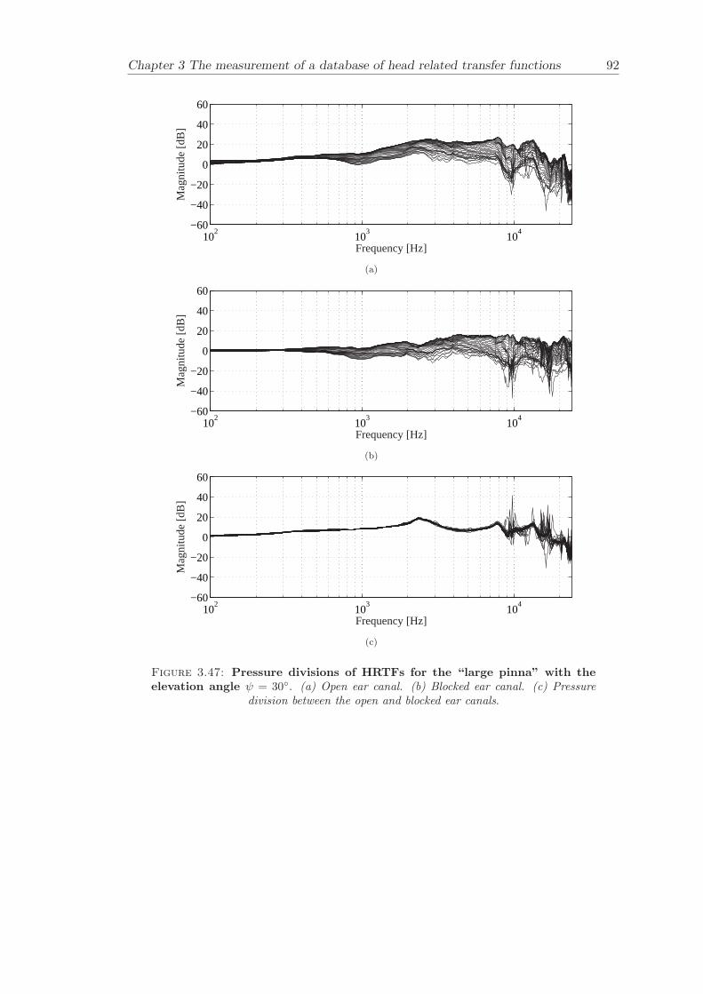
Chapter 3 The measurement of a database of head related transfer functions 92
102
103
104
−60
−40
−20
0
20
40
60
Frequency [Hz]
Mag
nitu
de [d
B]
(a)
102
103
104
−60
−40
−20
0
20
40
60
Frequency [Hz]
Mag
nitu
de [d
B]
(b)
102
103
104
−60
−40
−20
0
20
40
60
Frequency [Hz]
Mag
nitu
de [d
B]
(c)
Figure 3.47: Pressure divisions of HRTFs for the “large pinna” with theelevation angle ψ = 30. (a) Open ear canal. (b) Blocked ear canal. (c) Pressure
division between the open and blocked ear canals.
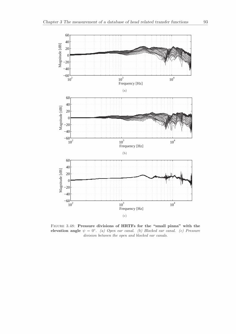
Chapter 3 The measurement of a database of head related transfer functions 93
102
103
104
−60
−40
−20
0
20
40
60
Frequency [Hz]
Mag
nitu
de [d
B]
(a)
102
103
104
−60
−40
−20
0
20
40
60
Frequency [Hz]
Mag
nitu
de [d
B]
(b)
102
103
104
−60
−40
−20
0
20
40
60
Frequency [Hz]
Mag
nitu
de [d
B]
(c)
Figure 3.48: Pressure divisions of HRTFs for the “small pinna” with theelevation angle ψ = 0. (a) Open ear canal. (b) Blocked ear canal. (c) Pressure
division between the open and blocked ear canals.
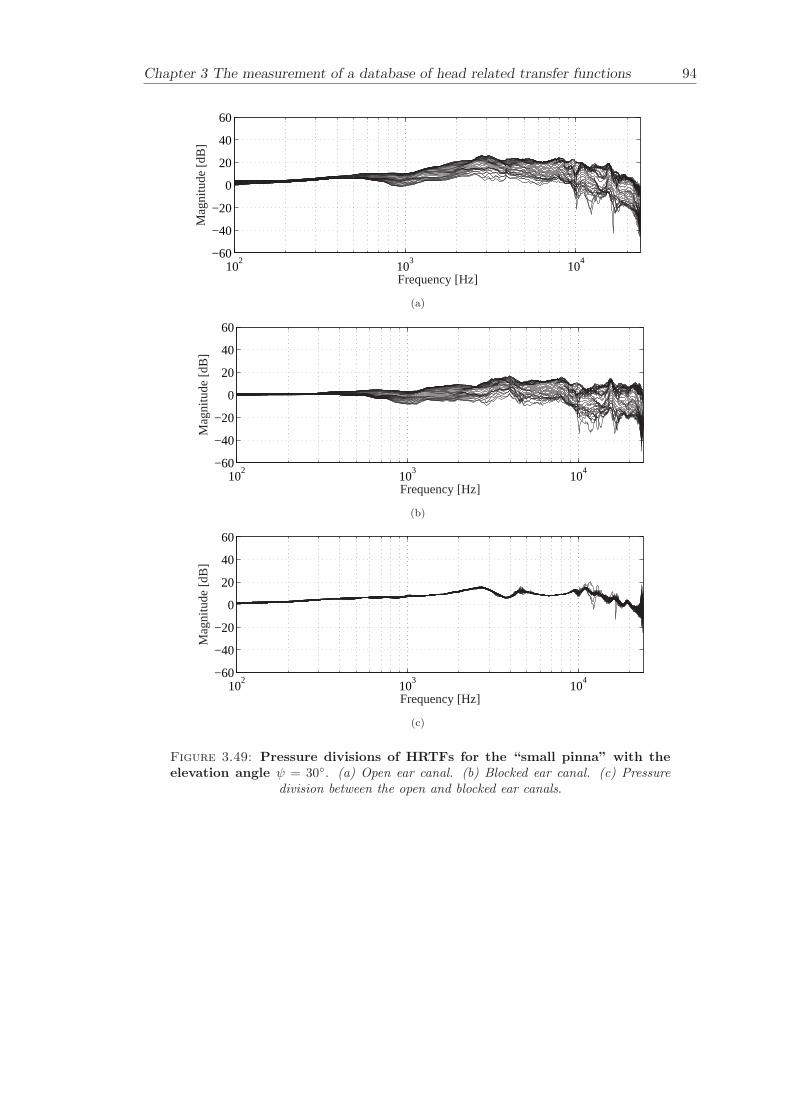
Chapter 3 The measurement of a database of head related transfer functions 94
102
103
104
−60
−40
−20
0
20
40
60
Frequency [Hz]
Mag
nitu
de [d
B]
(a)
102
103
104
−60
−40
−20
0
20
40
60
Frequency [Hz]
Mag
nitu
de [d
B]
(b)
102
103
104
−60
−40
−20
0
20
40
60
Frequency [Hz]
Mag
nitu
de [d
B]
(c)
Figure 3.49: Pressure divisions of HRTFs for the “small pinna” with theelevation angle ψ = 30. (a) Open ear canal. (b) Blocked ear canal. (c) Pressure
division between the open and blocked ear canals.
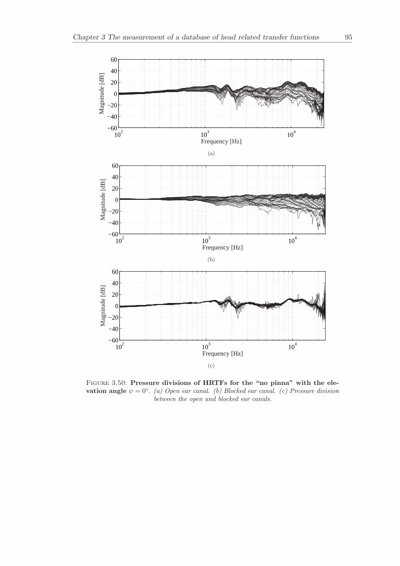
Chapter 3 The measurement of a database of head related transfer functions 95
102
103
104
−60
−40
−20
0
20
40
60
Frequency [Hz]
Mag
nitu
de [d
B]
(a)
102
103
104
−60
−40
−20
0
20
40
60
Frequency [Hz]
Mag
nitu
de [d
B]
(b)
102
103
104
−60
−40
−20
0
20
40
60
Frequency [Hz]
Mag
nitu
de [d
B]
(c)
Figure 3.50: Pressure divisions of HRTFs for the “no pinna” with the ele-vation angle ψ = 0. (a) Open ear canal. (b) Blocked ear canal. (c) Pressure division
between the open and blocked ear canals.
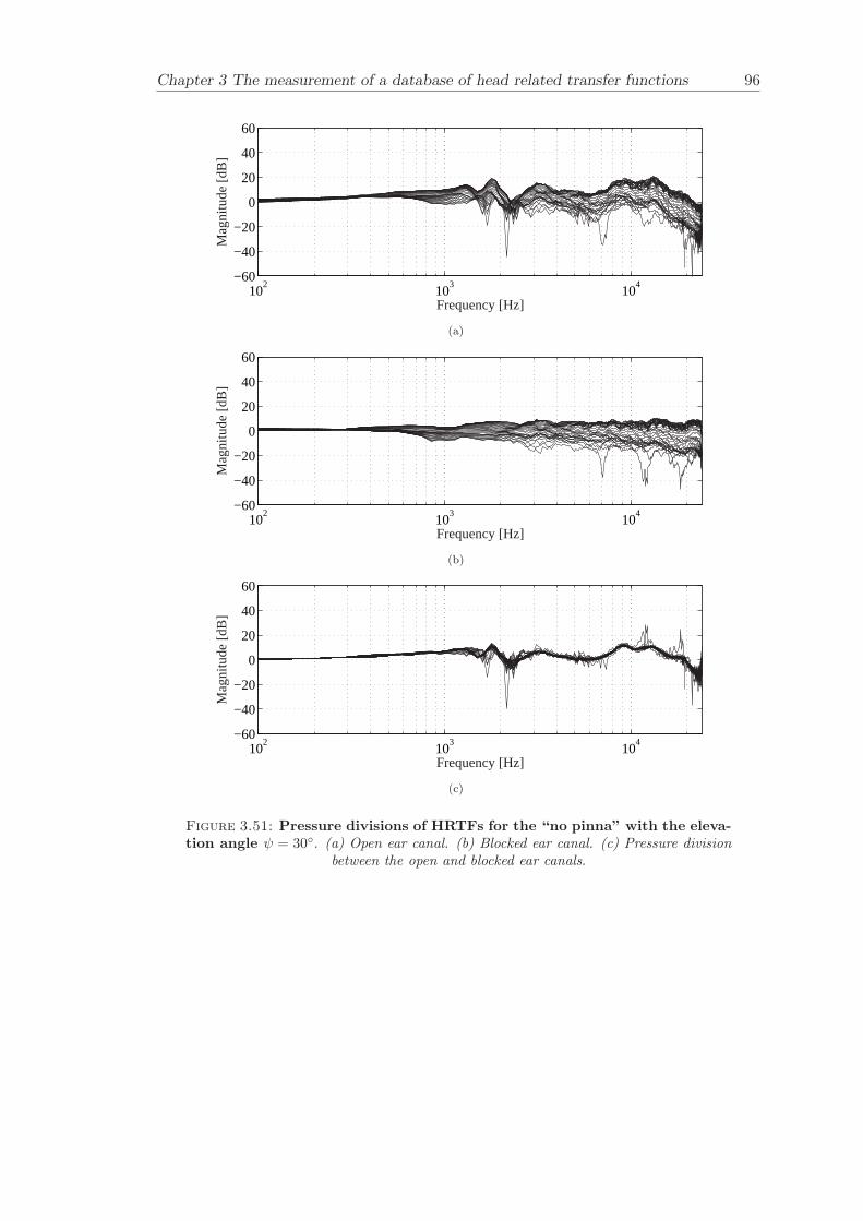
Chapter 3 The measurement of a database of head related transfer functions 96
102
103
104
−60
−40
−20
0
20
40
60
Frequency [Hz]
Mag
nitu
de [d
B]
(a)
102
103
104
−60
−40
−20
0
20
40
60
Frequency [Hz]
Mag
nitu
de [d
B]
(b)
102
103
104
−60
−40
−20
0
20
40
60
Frequency [Hz]
Mag
nitu
de [d
B]
(c)
Figure 3.51: Pressure divisions of HRTFs for the “no pinna” with the eleva-tion angle ψ = 30. (a) Open ear canal. (b) Blocked ear canal. (c) Pressure division
between the open and blocked ear canals.
Chapter 4
Interpolation of head related
impulse response functions
The filter update problem requires interpolation between HRIRs. A technique for linearinterpolation between mixed-phase HRIRs is presented in this chapter. The presentedinterpolation scheme uses ITD-equalisation and linear interpolation. The HRIR inter-polation is here performed in the time domain between neighbouring angular locations.The presented technique uses thresholding for the ITD-equalisation and is comparedto results presented by previous researchers. The ISVR-Samsung database that waspresented in the previous chapter is used in the objective evaluation carried out here.
Previous researchers have examined a number of interpolation techniques for HRTFs.Chen [18] proposes a feature extraction method, where the HRTF was represented asa weighted sum of Eigen transfer functions (EFs) generated by a Karhunen-Loeve ex-pansion (KLE). This approach, results in an error of less than 1% for interpolation ofmixed-phase HRTFs. Evan [28] presents a model where the HRTFs are representedas a weighted sum of surface spherical harmonics (SSHs). The interpolation perfor-mance is similar to the EF technique presented Chen [18]. However, the computationalefficiency of the SSH technique is inferior compared to the EF technique. Various inter-polation techniques including minimum-phase approximations are presented by Jot [44].Takeuchi [95] suggests a frequency domain method for interpolating HRTFs using mag-nitude and phase interpolation. The last two mentioned studies do not include anymeasure of the percentage error that their techniques imposes. The technique presentedby Takeuchi [95] is promising but there is no algorithm that wraps the phase correctlyas required included in this investigation. The interpolation technique introduced herethat uses thresholding is a robust and simple way to increase the resolution of a HRIRdatabase. The main advantage of this technique compared to Chen [18] is the inherentsimplicity.
There are three general techniques for extracting ITD information (Huopaniemi [38])
97
Chapter 4 Interpolation of head related impulse response functions 98
from HRIRs namely cross-correlation, thresholding (also known as leading-edge) andinteraural phase difference (IPD). The cross-correlation and thresholding techniques areuseful for deriving frequency independent ITD, while the IPD technique can include fre-quency dependent ITD values. The thresholding technique is evaluated in this Chapter.
4.1 Onset detection by thresholding
An interpolation algorithm that uses onset detection by thresholding for ITD-equalisationis introduced here. The ITD in the database is extracted by first using up-sampling fol-lowed by onset detection using thresholding. Ten times up-sampling has proven to bea good compromise between performance and computational effort. The up-samplingis applied to generate a higher resolution HRIR, which increases the precision in thetime-alignment step. The thresholding step is performed in order to time-align theHRIRs. The thresholding is performed by normalising all the HRIRs and detecting thestarting point of the HRIR at a threshold level of 0.1 of the maximum response. Nowlinear interpolation is applied in between the discrete measurement points for the timealigned HRIR database. The interpolation can either be applied in the time domainor in the frequency domain on the complex valued frequency response with equivalentresults. The delay that was removed in the thresholding step is inserted back again anddown-sampling is carried out to retrieve the database to its original size. It should benoted that the interpolation step can also be applied after down-sampling as long as thedatabase is still time-aligned.
The sample rate conversion (up-sampling and down-sampling) algorithms that have beenused here are described by Crochiere [23]. The original HRIR is denoted c(n) and theup-sampled HRIR is denoted y(m). The sampling rate is increased with an integer factorL and the new sampling period T
′is given by
T′
T=
1L
(4.1)
and the new sampling rate F′is given by
F′= LF (4.2)
The up-sampling of the impulse response c(n) by L implies that we must interpolateL − 1 new sample values between each pair of sample values of c(n). Figure 4.1 showsa diagram of the up-sampling process. The impulse response c(n) is zero padded withL−1 zero valued samples between each pair of samples of c(n), resulting in the followingsignal
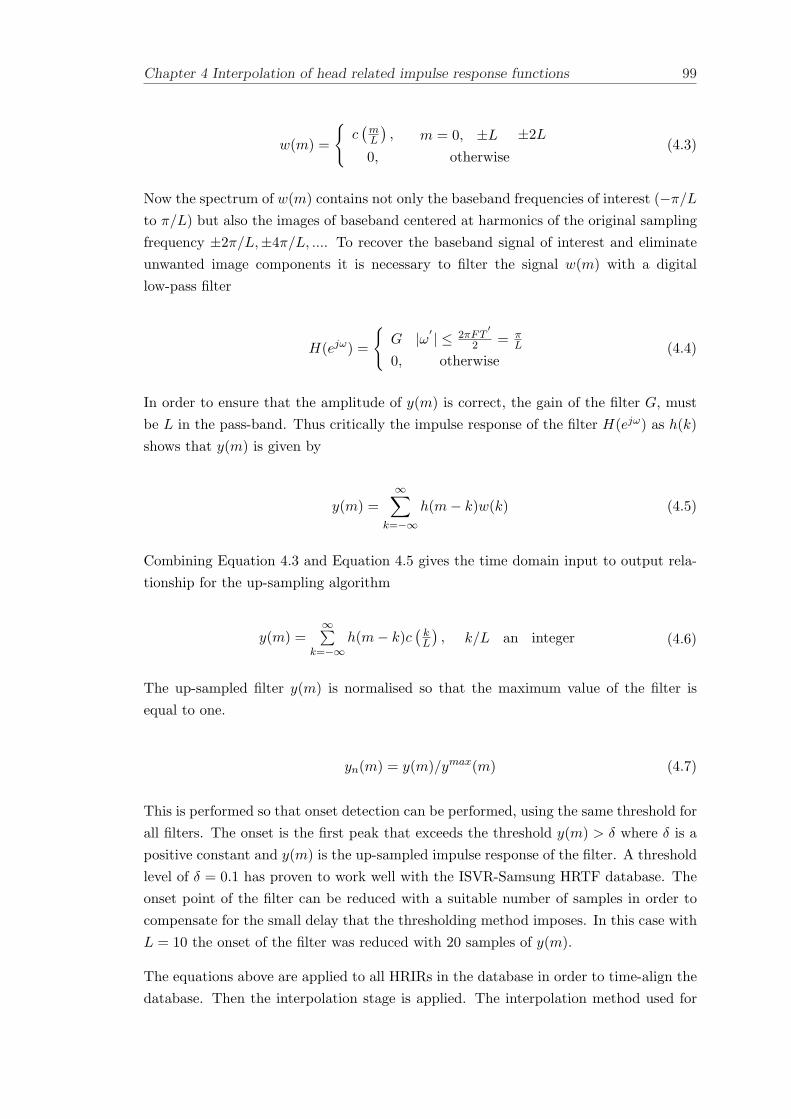
Chapter 4 Interpolation of head related impulse response functions 99
w(m) =
c(
mL
), m = 0, ±L ±2L
0, otherwise(4.3)
Now the spectrum of w(m) contains not only the baseband frequencies of interest (−π/L
to π/L) but also the images of baseband centered at harmonics of the original samplingfrequency ±2π/L,±4π/L, .... To recover the baseband signal of interest and eliminateunwanted image components it is necessary to filter the signal w(m) with a digitallow-pass filter
H(ejω) =
G |ω′ | ≤ 2πFT
′
2 = πL
0, otherwise(4.4)
In order to ensure that the amplitude of y(m) is correct, the gain of the filter G, mustbe L in the pass-band. Thus critically the impulse response of the filter H(ejω) as h(k)shows that y(m) is given by
y(m) =∞∑
k=−∞h(m− k)w(k) (4.5)
Combining Equation 4.3 and Equation 4.5 gives the time domain input to output rela-tionship for the up-sampling algorithm
y(m) =∞∑
k=−∞h(m− k)c
(kL
), k/L an integer (4.6)
The up-sampled filter y(m) is normalised so that the maximum value of the filter isequal to one.
yn(m) = y(m)/ymax(m) (4.7)
This is performed so that onset detection can be performed, using the same threshold forall filters. The onset is the first peak that exceeds the threshold y(m) > δ where δ is apositive constant and y(m) is the up-sampled impulse response of the filter. A thresholdlevel of δ = 0.1 has proven to work well with the ISVR-Samsung HRTF database. Theonset point of the filter can be reduced with a suitable number of samples in order tocompensate for the small delay that the thresholding method imposes. In this case withL = 10 the onset of the filter was reduced with 20 samples of y(m).
The equations above are applied to all HRIRs in the database in order to time-align thedatabase. Then the interpolation stage is applied. The interpolation method used for
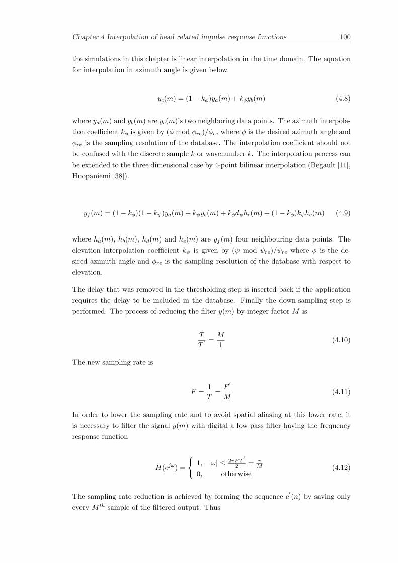
Chapter 4 Interpolation of head related impulse response functions 100
the simulations in this chapter is linear interpolation in the time domain. The equationfor interpolation in azimuth angle is given below
yc(m) = (1− kφ)ya(m) + kφyb(m) (4.8)
where ya(m) and yb(m) are yc(m)’s two neighboring data points. The azimuth interpola-tion coefficient kφ is given by (φ mod φre)/φre where φ is the desired azimuth angle andφre is the sampling resolution of the database. The interpolation coefficient should notbe confused with the discrete sample k or wavenumber k. The interpolation process canbe extended to the three dimensional case by 4-point bilinear interpolation (Begault [11],Huopaniemi [38]).
yf (m) = (1− kφ)(1− kψ)ya(m) + kψyb(m) + kφdψhc(m) + (1− kφ)kψhe(m) (4.9)
where ha(m), hb(m), hd(m) and he(m) are yf (m) four neighbouring data points. Theelevation interpolation coefficient kψ is given by (ψ mod ψre)/ψre where φ is the de-sired azimuth angle and φre is the sampling resolution of the database with respect toelevation.
The delay that was removed in the thresholding step is inserted back if the applicationrequires the delay to be included in the database. Finally the down-sampling step isperformed. The process of reducing the filter y(m) by integer factor M is
T
T ′ =M
1(4.10)
The new sampling rate is
F =1T
=F′
M(4.11)
In order to lower the sampling rate and to avoid spatial aliasing at this lower rate, itis necessary to filter the signal y(m) with digital a low pass filter having the frequencyresponse function
H(ejω) =
1, |ω| ≤ 2πFT
′
2 = πM
0, otherwise(4.12)
The sampling rate reduction is achieved by forming the sequence c′(n) by saving only
every M th sample of the filtered output. Thus
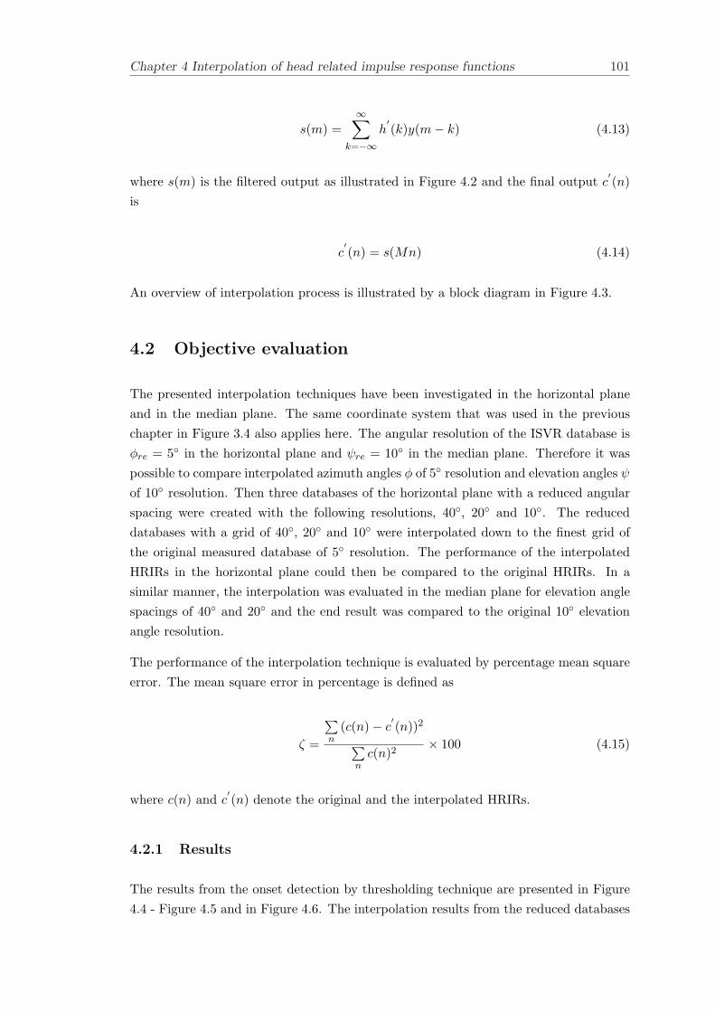
Chapter 4 Interpolation of head related impulse response functions 101
s(m) =∞∑
k=−∞h′(k)y(m− k) (4.13)
where s(m) is the filtered output as illustrated in Figure 4.2 and the final output c′(n)
is
c′(n) = s(Mn) (4.14)
An overview of interpolation process is illustrated by a block diagram in Figure 4.3.
4.2 Objective evaluation
The presented interpolation techniques have been investigated in the horizontal planeand in the median plane. The same coordinate system that was used in the previouschapter in Figure 3.4 also applies here. The angular resolution of the ISVR database isφre = 5 in the horizontal plane and ψre = 10 in the median plane. Therefore it waspossible to compare interpolated azimuth angles φ of 5 resolution and elevation angles ψ
of 10 resolution. Then three databases of the horizontal plane with a reduced angularspacing were created with the following resolutions, 40, 20 and 10. The reduceddatabases with a grid of 40, 20 and 10 were interpolated down to the finest grid ofthe original measured database of 5 resolution. The performance of the interpolatedHRIRs in the horizontal plane could then be compared to the original HRIRs. In asimilar manner, the interpolation was evaluated in the median plane for elevation anglespacings of 40 and 20 and the end result was compared to the original 10 elevationangle resolution.
The performance of the interpolation technique is evaluated by percentage mean squareerror. The mean square error in percentage is defined as
ζ =
∑n
(c(n)− c′(n))2
∑n
c(n)2× 100 (4.15)
where c(n) and c′(n) denote the original and the interpolated HRIRs.
4.2.1 Results
The results from the onset detection by thresholding technique are presented in Figure4.4 - Figure 4.5 and in Figure 4.6. The interpolation results from the reduced databases
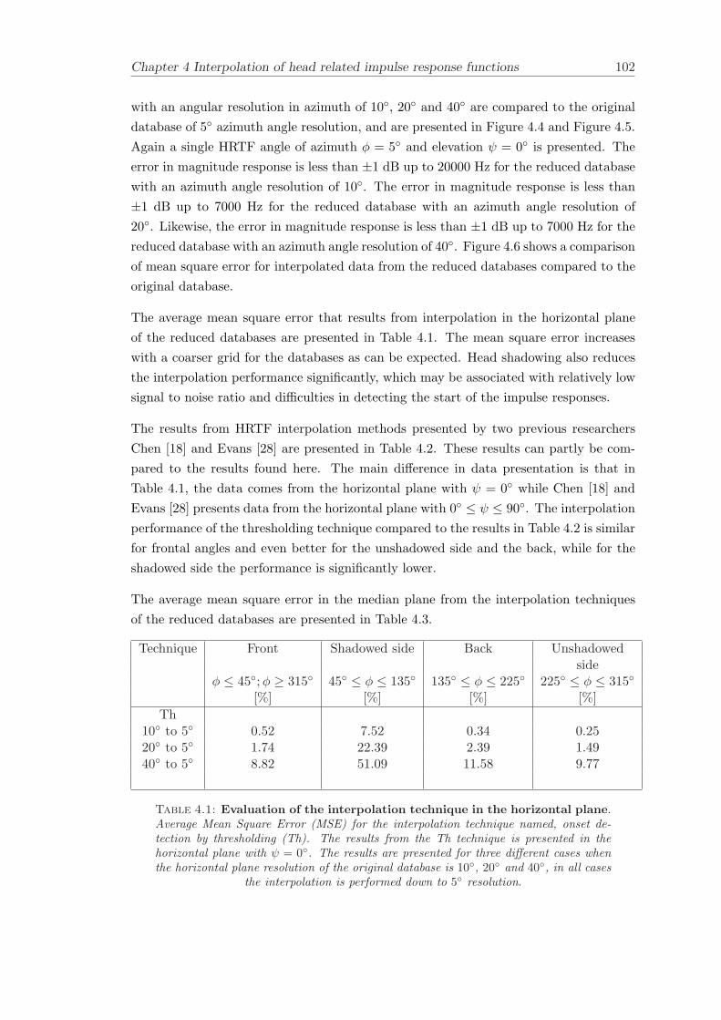
Chapter 4 Interpolation of head related impulse response functions 102
with an angular resolution in azimuth of 10, 20 and 40 are compared to the originaldatabase of 5 azimuth angle resolution, and are presented in Figure 4.4 and Figure 4.5.Again a single HRTF angle of azimuth φ = 5 and elevation ψ = 0 is presented. Theerror in magnitude response is less than ±1 dB up to 20000 Hz for the reduced databasewith an azimuth angle resolution of 10. The error in magnitude response is less than±1 dB up to 7000 Hz for the reduced database with an azimuth angle resolution of20. Likewise, the error in magnitude response is less than ±1 dB up to 7000 Hz for thereduced database with an azimuth angle resolution of 40. Figure 4.6 shows a comparisonof mean square error for interpolated data from the reduced databases compared to theoriginal database.
The average mean square error that results from interpolation in the horizontal planeof the reduced databases are presented in Table 4.1. The mean square error increaseswith a coarser grid for the databases as can be expected. Head shadowing also reducesthe interpolation performance significantly, which may be associated with relatively lowsignal to noise ratio and difficulties in detecting the start of the impulse responses.
The results from HRTF interpolation methods presented by two previous researchersChen [18] and Evans [28] are presented in Table 4.2. These results can partly be com-pared to the results found here. The main difference in data presentation is that inTable 4.1, the data comes from the horizontal plane with ψ = 0 while Chen [18] andEvans [28] presents data from the horizontal plane with 0 ≤ ψ ≤ 90. The interpolationperformance of the thresholding technique compared to the results in Table 4.2 is similarfor frontal angles and even better for the unshadowed side and the back, while for theshadowed side the performance is significantly lower.
The average mean square error in the median plane from the interpolation techniquesof the reduced databases are presented in Table 4.3.
Technique Front Shadowed side Back Unshadowedside
φ ≤ 45; φ ≥ 315 45 ≤ φ ≤ 135 135 ≤ φ ≤ 225 225 ≤ φ ≤ 315
[%] [%] [%] [%]Th
10 to 5 0.52 7.52 0.34 0.2520 to 5 1.74 22.39 2.39 1.4940 to 5 8.82 51.09 11.58 9.77
Table 4.1: Evaluation of the interpolation technique in the horizontal plane.Average Mean Square Error (MSE) for the interpolation technique named, onset de-tection by thresholding (Th). The results from the Th technique is presented in thehorizontal plane with ψ = 0. The results are presented for three different cases whenthe horizontal plane resolution of the original database is 10, 20 and 40, in all cases
the interpolation is performed down to 5 resolution.
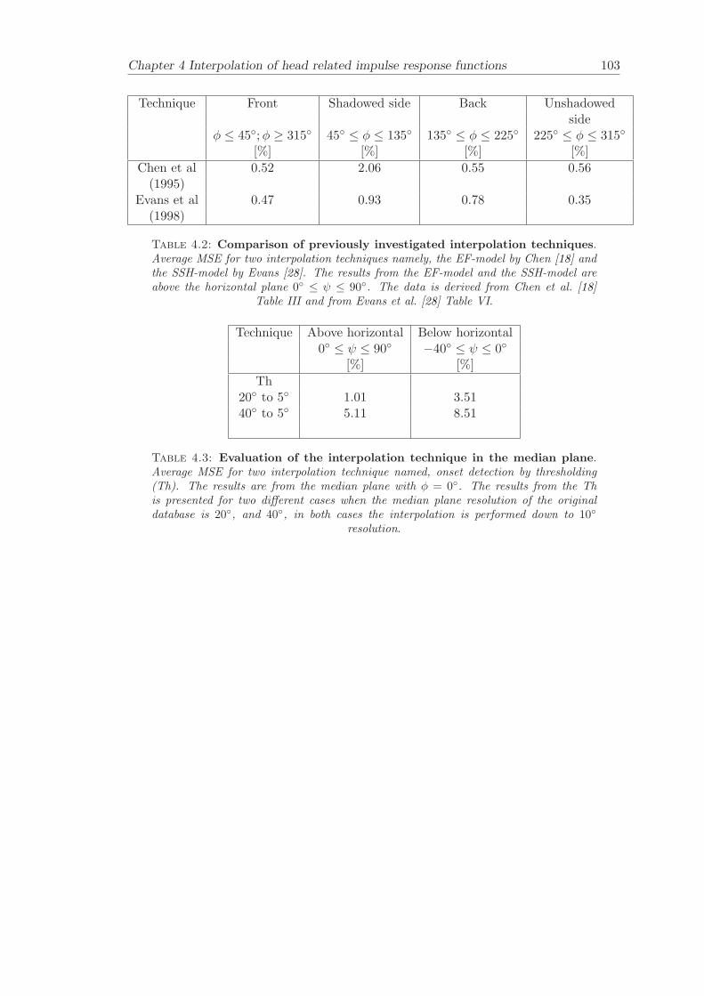
Chapter 4 Interpolation of head related impulse response functions 103
Technique Front Shadowed side Back Unshadowedside
φ ≤ 45; φ ≥ 315 45 ≤ φ ≤ 135 135 ≤ φ ≤ 225 225 ≤ φ ≤ 315
[%] [%] [%] [%]Chen et al 0.52 2.06 0.55 0.56
(1995)Evans et al 0.47 0.93 0.78 0.35
(1998)
Table 4.2: Comparison of previously investigated interpolation techniques.Average MSE for two interpolation techniques namely, the EF-model by Chen [18] andthe SSH-model by Evans [28]. The results from the EF-model and the SSH-model areabove the horizontal plane 0 ≤ ψ ≤ 90. The data is derived from Chen et al. [18]
Table III and from Evans et al. [28] Table VI.
Technique Above horizontal Below horizontal0 ≤ ψ ≤ 90 −40 ≤ ψ ≤ 0
[%] [%]Th
20 to 5 1.01 3.5140 to 5 5.11 8.51
Table 4.3: Evaluation of the interpolation technique in the median plane.Average MSE for two interpolation technique named, onset detection by thresholding(Th). The results are from the median plane with φ = 0. The results from the This presented for two different cases when the median plane resolution of the originaldatabase is 20, and 40, in both cases the interpolation is performed down to 10
resolution.
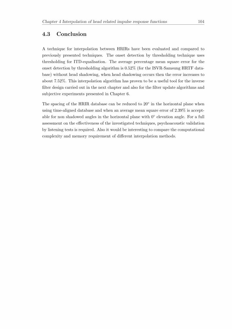
Chapter 4 Interpolation of head related impulse response functions 104
4.3 Conclusion
A technique for interpolation between HRIRs have been evaluated and compared topreviously presented techniques. The onset detection by thresholding technique usesthresholding for ITD-equalisation. The average percentage mean square error for theonset detection by thresholding algorithm is 0.52% (for the ISVR-Samsung HRTF data-base) without head shadowing, when head shadowing occurs then the error increases toabout 7.52%. This interpolation algorithm has proven to be a useful tool for the inversefilter design carried out in the next chapter and also for the filter update algorithms andsubjective experiments presented in Chapter 6.
The spacing of the HRIR database can be reduced to 20 in the horizontal plane whenusing time-aligned database and when an average mean square error of 2.39% is accept-able for non shadowed angles in the horizontal plane with 0 elevation angle. For a fullassessment on the effectiveness of the investigated techniques, psychoacoustic validationby listening tests is required. Also it would be interesting to compare the computationalcomplexity and memory requirement of different interpolation methods.
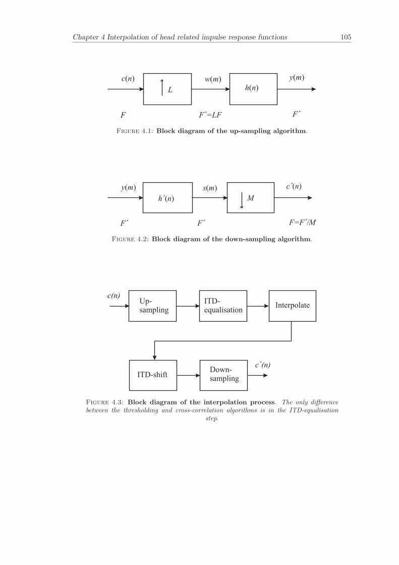
Chapter 4 Interpolation of head related impulse response functions 105
L
c n( ) w m( ) y m( )
h n( )
F F =LF´ F´
Figure 4.1: Block diagram of the up-sampling algorithm.
h n´( )
y m( ) s m( ) c n´( )
M
F´ F´ F=F /M´
Figure 4.2: Block diagram of the down-sampling algorithm.
c(n)ITD-equalisation
Up-sampling
Interpolate
ITD-shiftDown-sampling
c (n)´
Figure 4.3: Block diagram of the interpolation process. The only differencebetween the thresholding and cross-correlation algorithms is in the ITD-equalisation
step.
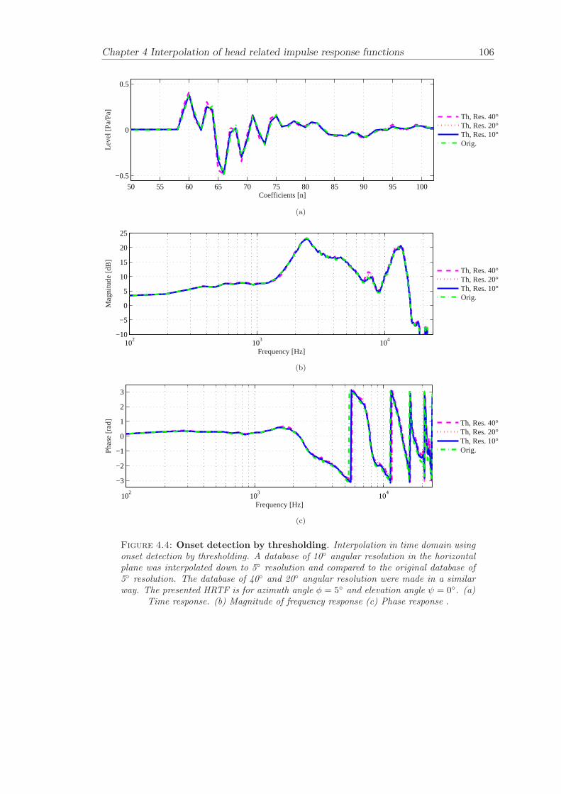
Chapter 4 Interpolation of head related impulse response functions 106
50 55 60 65 70 75 80 85 90 95 100
−0.5
0
0.5
Leve
l [P
a/P
a]
Coefficients [n]
Th, Res. 40°Th, Res. 20°Th, Res. 10°Orig.
(a)
102
103
104
−10
−5
0
5
10
15
20
25
Mag
nitu
de [d
B]
Frequency [Hz]
Th, Res. 40°Th, Res. 20°Th, Res. 10°Orig.
(b)
102
103
104
−3
−2
−1
0
1
2
3
Pha
se [r
ad]
Frequency [Hz]
Th, Res. 40°Th, Res. 20°Th, Res. 10°Orig.
(c)
Figure 4.4: Onset detection by thresholding. Interpolation in time domain usingonset detection by thresholding. A database of 10 angular resolution in the horizontalplane was interpolated down to 5 resolution and compared to the original database of5 resolution. The database of 40 and 20 angular resolution were made in a similarway. The presented HRTF is for azimuth angle φ = 5 and elevation angle ψ = 0. (a)
Time response. (b) Magnitude of frequency response (c) Phase response .
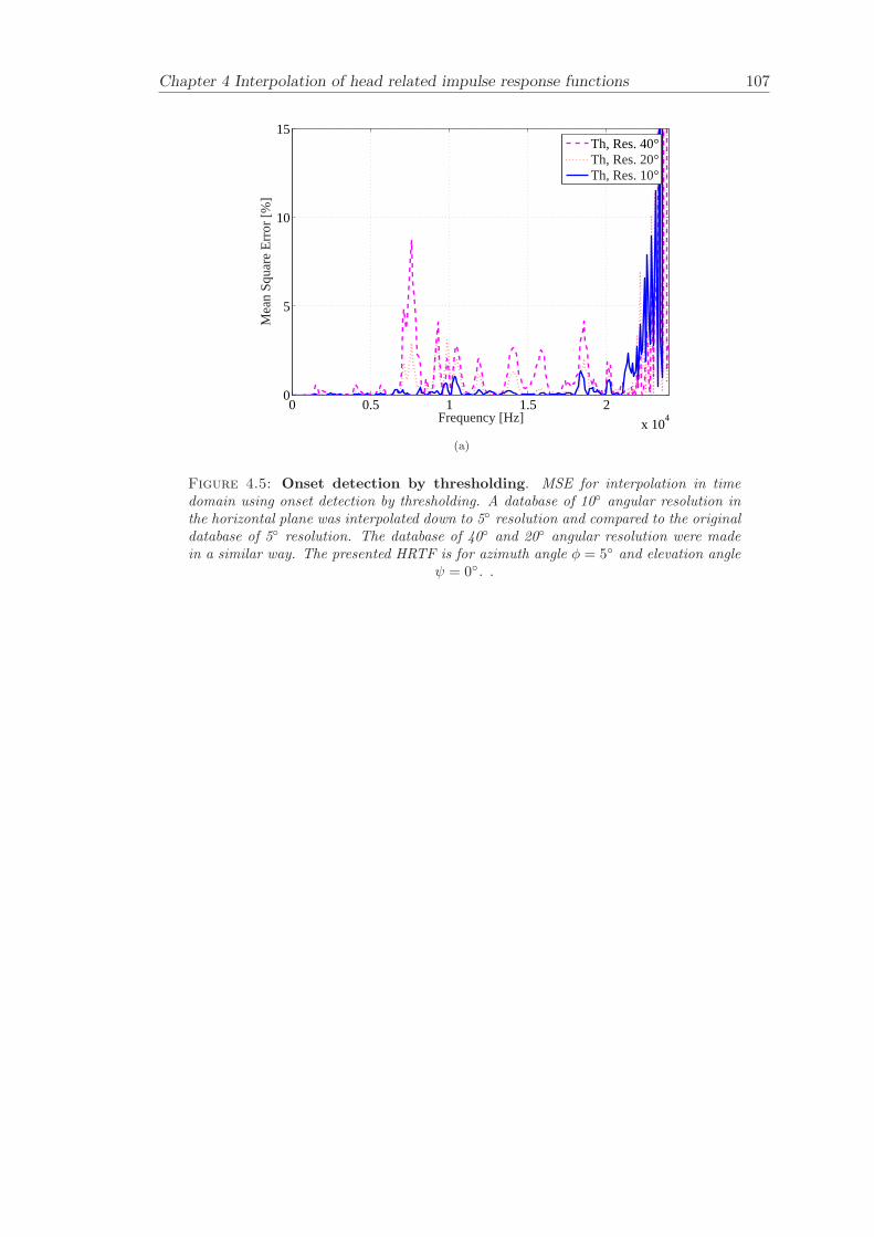
Chapter 4 Interpolation of head related impulse response functions 107
0 0.5 1 1.5 2
x 104
0
5
10
15
Frequency [Hz]
Mea
n S
quar
e E
rror
[%]
Th, Res. 40°Th, Res. 20°Th, Res. 10°
(a)
Figure 4.5: Onset detection by thresholding. MSE for interpolation in timedomain using onset detection by thresholding. A database of 10 angular resolution inthe horizontal plane was interpolated down to 5 resolution and compared to the originaldatabase of 5 resolution. The database of 40 and 20 angular resolution were madein a similar way. The presented HRTF is for azimuth angle φ = 5 and elevation angle
ψ = 0. .
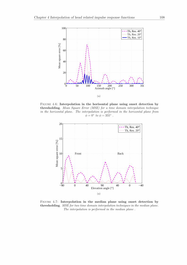
Chapter 4 Interpolation of head related impulse response functions 108
0 50 100 150 200 250 300 3500
20
40
60
80
100
Azimuth angle [°]
Mea
n sq
uare
err
or [%
]
Th, Res. 40°Th, Res. 20°Th, Res. 10°
(a)
Figure 4.6: Interpolation in the horisontal plane using onset detection bythresholding. Mean Square Error (MSE) for a time domain interpolation techniquein the horizontal plane. The interpolation is performed in the horizontal plane from
φ = 0 to φ = 355 .
−40 0 40 90 40 0 −400
5
10
15
20
Elevation angle [°]
Mea
n sq
uare
err
or [%
]
Front Back
Th, Res. 40°Th, Res. 20°
(a)
Figure 4.7: Interpolation in the median plane using onset detection bythresholding. MSE for two time domain interpolation techniques in the median plane.
The interpolation is performed in the median plane .
Chapter 5
Filter design and the effectiveness
of cross-talk cancellation
This chapter presents filter design techniques and an objective evaluation of cross-talkcancellation effectiveness for three virtual sound imaging systems, namely the SD, 2-wayOSD and the 3-way OSD. It is shown how the geometry affects the filter design processand how to design the cross-talk cancellation networks using a minimum number ofinverse filters. The filter design for OSD systems can be simplified by using superposi-tion. This gives the advantage of reducing the number of inverse filters for the OSD tothe same number as for the SD. The objective evaluation is carried out by simulatingcross-talk cancellation effectiveness for different filter lengths and for asymmetric andsymmetric listener positions of static and adaptive systems. The evaluation of cross talkcancellation effectiveness for different filter lengths aims to give an idea of which filterlength to choose for a certain performance requirement. The benefit of using an adap-tive virtual sound imaging system compared to a static virtual sound imaging system isdemonstrated. The effectiveness of cross talk cancellation when using a static system isrestricted to a relatively small area named the “sweet-spot”. The improvements in areasize where the listener can move, using an adaptive approach and steering the associatedsweet-spot, is compared to the static case.
The evaluation is performed by simulations using measurement data from the anechoicchamber at the ISVR. The transfer functions used in the simulations both for the adap-tive and the static systems include the HRTF and the loudspeaker response. This aimsto evaluate the cross talk cancellation effectiveness under anechoic conditions. Cross-overs are included in the filter length evaluation but not included in the simulations ofadaptive and the static systems. The simulations of adaptive and the static systems areperformed for discrete sources and then the frequency band of each source are plottedtogether to show the full frequency band. The effect of fixed and adaptive cross-oversfor adaptive systems are not included in the objective evaluation presented here.
109
Chapter 5 Filter design and the effectiveness of cross-talk cancellation 110
The theory of cross-talk cancellation was introduced by Bauer [10] in an analogue imple-mentation and followed up by Atal and Schroeder [4]. More recently, cross-talk cancel-lation techniques has been investigated by a number of researchers such as, Moller [68],Cooper and Bauck [20], Gardner [30], Kirkeby and Nelson [50], Ward and Elko [100]and Takeuchi [95]. Ward and Elko [100] showed that the transfer function matrix tobe inverted became ill-conditioned when the path-length difference between one of theloudspeakers and two of the ears of the listener became equal to one half of the acousticwavelength. This led to the development of the SD (Kirkeby and Nelson [49]), whichensured a well-conditioned inversion problem over a particularly useful frequency range.It was pointed out by Ward and Elko [100] that for broadband signals, ideally theloudspeaker spacing should vary with frequency. This theory was extended further byTakeuchi [95], [97] who presented the OSD loudspeaker and conducted a set of subjectiveexperiments that showed the improvements in virtual sound source localisation that canbe achieved with this loudspeaker type. Previous studies did not include the theory forhow to design cross-talk cancellation filters for an OSD system using a minimum numberof inverse filters, and this is presented here.
Different methods of loudspeaker response equalization using digital filters are com-pared by Karjalainen [45]. The advantages of Warped Finite Impulse Response (WFIR)and Warped Infinite Impulse Response (WIIR) filters are shown in comparison withtraditional filter structures and are found to give a reduced filter order and increasednumerical robustness. The disadvantage is the higher computational complexity of thewarped structures. The required filter length for efficient cross-talk cancellation has pre-viously been investigated by Farina [29]. Farina has implemented WFIRs for cross-talkcancellation and demonstrated the low frequency benefits and filter order reduction ofsuch an approach. This chapter compares the cross-talk cancellation performance forthe SD, 2-way OSD and the 3-way OSD. The filter design technique used here is theone presented by Kirkeby [50] and can be implemented using Finite Impulse Response(FIR) filters.
A subjective investigation of inverse filtering is presented by Norcross [79]. The ideawith inverse filtering is to undo the filtering caused by a system such as a loudspeaker ora room. The inversion of an impulse response might cause undesired audible artefactsand the severity of these artefacts is affected by the impulse response of the systemand the method used to compute the inverse filter. The artefacts from the inversefiltering can some times degrade the overall signal quality instead of improving it. Thisstudy has presented formal subjective tests to investigate potential limitations associatedwith inverse filtering techniques. The investigated inverse filtering techniques are thetime domain least square (LS)-technique and frequency domain methods including thefast-deconvolution algorithm, both by Kirkeby and Nelson [50], [48]. Their subjectiveresults show that the investigated inverse filtering techniques can sometimes improvethe subjective audio quality and in other cases degrade it. The subjective audio quality
Chapter 5 Filter design and the effectiveness of cross-talk cancellation 111
depends on the impulse response, the chosen filtering technique and on the inverse filterlength.
The robustness to head misalignment for cross-talk cancellation using the converted (60
loudspeaker span) stereo configuration was investigated by Gardner [30] and the SD andStereo configuration was investigated by Takeuchi [96]. Misalignment of the head posi-tion and orientation give rise to inaccurate synthesis of the binaural signals at the ears ofthe listener. This is because the change in transfer functions between the loudspeakersand listener’s ears and the result is deterioration in system performance. To overcomethe limitations in “sweet-spot” size Rose [86] investigated an adaptive SD system, wherethe change in transfer function is compensated for by adapting the cross-talk cancella-tion scheme to the position and orientation of the listener. This study includes objectiveand subjective evaluations of cross-talk cancellation effectiveness in the lateral plane forthe SD. In this chapter an objective evaluation of cross-talk cancellation effectivenessis presented for the SD, 2-way OSD and the 3-way OSD for the lateral plane, fore andaft plane and listener rotation together with filter lengths dependency and filter designtechniques.
5.1 Filter design for virtual sound imaging systems
The solution to the problem of using a minimum number of inverse filters when designingfilters for a FDL is to use superposition. This results in the same number of filters for theFDL as for a two-channel loudspeaker system like the SD. For example, without usingsuperposition in the filter design process one would need a set of filters per transducerspan, hence the 3-way OSD would need three times more filters than the SD. The filterdesign process for binaural loudspeakers systems using the minimum number of inversefilters is described for the following three examples, namely the SD, the 2-way OSD andthe 3-way OSD.
The impulse responses for the SD are found by taking the impulse responses from az-imuth angles 355 and 5 for the left and the right ear respectively. The transfer functions(C11(k), C12(k), C21(k) and C22(k)) and the source angle α1 for the SD are presentedin Figure 5.5. The transfer function matrix C(k) is given by
C(k) =
[C11(k) C12(k)C21(k) C22(k)
](5.1)
and the inverse of C(k) is
H(k) ≈ C−1(k)e−jω∆ (5.2)
Chapter 5 Filter design and the effectiveness of cross-talk cancellation 112
The combined transfer functions (D11(k), D12(k), D21(k) and D22(k)), cross-overs (G11(k),G12(k), G21(k) and G22(k)) and the source angles (σ1 and σ2) for the 2-way OSD arepresented in Figure 5.5. The transfer function paths including cross-overs can be addedtogether using superposition (Pierce [83]). To find the combined transfer functions, thefollowing equations are used
D11(k) = D11,1(k)G11(k) + D11,2(k)G12(k) (5.3)
D12(k) = D12,1(k)G21(k) + D12,2(k)G22(k) (5.4)
D21(k) = D21,1(k)G11(k) + D21,2(k)G12(k) (5.5)
D22(k) = D22,1(k)G21(k) + D22,2(k)G22(k) (5.6)
The combined transfer function matrix D(k) is given by
D(k) =
[D11(k) D12(k)D21(k) D22(k)
](5.7)
and the inverse of D(k) is
J(k) ≈ D−1(k)e−jω∆ (5.8)
Using the combined transfer functions, results in less effort to compute the inversetransfer functions, since otherwise one would need to compute inverse filters for all thecomponents in Equations 5.3 - 5.6. Without using superposition one would also needtwice the number of filters in the convolution engine.
The combined transfer functions (E11(k), E12(k), E21(k) and E22(k)), cross-overs (F11(k),F12(k), F13(k), F21(k), F22(k), F23(k)) and the source angles (ϕ1, ϕ2 and ϕ3) for the3-way OSD are presented in Figure 5.3. The transfer function paths can be added to-gether using superposition, using the same method as for the 2-way OSD. To find thecombined transfer functions, the following equations are used
E11(k) = E11,1(k)F11(k) + E11,2(k)F12(k) + E11,3(k)F13(k) (5.9)
E12(k) = E12,1(k)F21(k) + E12,2(k)F22(k) + E12,3(k)F23(k) (5.10)
E21(k) = E21,1(k)F11(k) + E21,2(k)F12(k) + E21,3(k)F13(k) (5.11)
E22(k) = E22,1(k)F21(k) + E22,2(k)F22(k) + E22,3(k)F23(k) (5.12)
The combined transfer function matrix E(k) is given by
Chapter 5 Filter design and the effectiveness of cross-talk cancellation 113
E(k) =
[E11(k) E12(k)E21(k) E22(k)
](5.13)
and the inverse of E(k) is
K(k) ≈ E−1(k)e−jω∆ (5.14)
Again, by using the combined transfer functions in Equations 5.9 - 5.12, results in lesseffort to compute the inverse transfer functions. In this case, without using superpositionone would need triple the number of filters in the convolution engine.
5.2 Filter length dependency
The effectiveness of cross talk cancellation for different filter lengths is an importantissue. Cross-talk cancellation effectiveness for the SD, 2-way OSD and the 3-way OSDusing different filter lengths is evaluated under anechoic conditions. The data used inthis objective evaluation is based on the raw impulse responses that were obtained duringISVR-Samsung HRTF database measurement. The raw impulse response contains 4096coefficients and includes the loudspeaker response and the KEMAR dummy head HRTFfrom the “large pinna”. The plant model that was used contains 3000 filter coefficients ofthe raw impulse responses. The cross-overs were designed using the Matlab [66] functionfir1() that implements the classical method of windowed linear-phase FIR filters [40](Hann-window based). The cross-over frequency for the 2-way OSD is at 900 Hz, whichis illustrated in Figure 2.8. The cross-over frequencies for the 3-way OSD are at 4000 Hzand 600 Hz, which is illustrated in Figure 2.6. The inverse of the transfer functions werefound by using the fast-deconvolution algorithm. The regularisation factor β in the fast-deconvolution algorithm was set to 10−4 according to suggestions made by Kirkeby [50].The same β value was used for all the three virtual sound imaging systems and only thenumber of coefficients in the filter was varied. Inverse filters with different number ofcoefficients N (32, 64, 128, 256, 512, 1048, 2048, 4096, 8192, 16384) were designed. Theperformance of the inverse filters with different numbers of coefficients was evaluatedby simulating cross-talk cancellation effectiveness for the three virtual sound imagingsystems.
The transfer functions and inverse transfer function are defined as in Section 5.1. The SDis associated with C(k), the 2-way OSD is associated D(k) and 3-way OSD is associatedE(k). In the same manner, the inverse transfer functions for the SD, 2-way OSD andthe 3-way OSD are defined as H(k), J(k) and K(k) respectively. For the SD, the firstNi coefficients of the matrix of transfer functions C(k) is named CNi(k) and the inversematrix of CNi(k) is named HN (k). The inverse transfer functions HN (k) are found by
Chapter 5 Filter design and the effectiveness of cross-talk cancellation 114
zero padding CNi(k) up to N = 4Ni coefficients and then using the fast-deconvolutionalgorithm. The number of coefficients of the impulse response Ni was varied (8, 16,32, 64, 128, 256, 512, 1024, 2048). The inverse filter with N = 16384 was calculatedusing Ni = 2048 to make sure that Ni was not longer than the plant model of 3000coefficients. The reason to choose N = 4Ni was to minimize “wrap around” effects inthe FFTs when carrying out fast-deconvolution. The plant model CNp(k) that was usedcontains Np = 3000 coefficients of the transfer functions with a Hann-window applied,in order to suppress noise in the late response. The plant model aims to give a realisticobjective evaluation of the system. The matrix of transfer functions, inverse matrix andplant model for the 2-way OSD and 3-way OSD are found in the same way as describedfor the SD.
The results from simulated cross-talk cancellation performance using measured transferfunctions are presented for inverse filters with different number of coefficients. Thesimulated cross-talk performance is plotted in Figure 5.4 - Figure 5.9. Figure 5.4, Figure5.5 and Figure 5.6 illustrates the control performance in the frequency domain P11(k)and P21(k) at the ears, as specified in Equation 2.30. The control performance in thefrequency domain is also summarised in Table 5.1. Figure 5.7, Figure 5.8 and Figure 5.9illustrates the control performance in the time domain p11(n) and p21(n) at the ears, asspecified in Equation 2.30 and Equation 2.31. The impulse responses p11(n) and p21(n)are plotted using the decibel scale.
The channel separation parameter is used as a measure of cross-talk cancellation effec-tiveness. The channel separation in dB is defined as the ratio of the magnitude of thecontrol performance at the ears.
S(k) = 20 log10
( |P11(k)||P21(k)|
)(5.15)
The bandwidth dependence of the number of filter coefficients is presented in Table 5.1.The bandwidth is here found by defining a minimum required channel separation ofS(k) > 20 dB. It can be seen that the upper limit of the 2-way OSD is higher comparedto the 3-way OSD, this can be because the HRTFs for the 6 source span contain onlya small amount of energy in the highest frequencies. If one attempts to invert such atransfer function, the solution will boost frequencies just below the Nyquist frequency,which can reduce the cross-talk cancellation effectiveness.
Norcross [79] concluded that artefacts above -50 dB in the noise floor produced delay-type effects that where clearly audible to the subjects. Though the referenced studywas made on a 1-channel inversion problem and the problem addressed here is 2-channelinversion, one would expect that the level of artefacts in the noise floor of the 1-channelsystem will still be audible in the 2-channel inversion case. The results in Table 5.2indicates that the minimum filter length for not producing any audible artefacts using
Chapter 5 Filter design and the effectiveness of cross-talk cancellation 115
Number of Bandwidth Bandwidth Bandwidthcoefficients SD 2-way OSD 3-way OSD
S(k) > 20 dB S(k) > 20 dB S(k) > 20 dB[Hz] [Hz] [Hz]
32 - - -64 - - -128 - - -256 - - -512 2000-6000 2000-5000 4000-160001024 900-6000 2000-5000 4000-160002048 900-8000 1000-8000 700-160004096 800-8000 100-20000 50-160008192 800-19000 100-20000 30-1600016384 700-19000 100-20000 30-16000
Table 5.1: Control performance for different filter lengths and systems.
the -50 dB limit is 4096 coefficients for all three systems.
Number of Noise floor Noise floor Noise floorcoefficients SD 2-way OSD 3-way OSD
[dB] [dB] [dB]32 -10 -10 -1064 -10 -20 -15128 -20 -20 -20256 -25 -30 -30512 -35 -40 -401024 -40 -40 -402048 -40 -40 -404096 -50 -55 -558192 -55 -60 -5516384 -55 -60 -55
Table 5.2: Noise floor for different filter lengths and systems.
5.3 Cross-talk cancellation effectiveness
The effectiveness of cross-talk cancellation depends partly on the position of the listenerand whether the system is static or adaptive. The evaluation is performed in the lateralplane (asymmetric), the fore and aft plane (symmetric) and for rotation (asymmetric).The listening position was moved from −1 ≤ X ≤ 1 m in the lateral plane (Z = 0) andfrom −1 ≤ Z ≤ 1 m (X = 0 m) in the fore and aft plane both with a step size of 0.01 m.The evaluation of listener rotation was performed by rotating the listener position from0 to 90 in 1 steps. The evaluation is carried out for the static case and the adaptivecase. In the static system, the cross talk cancellation filters are not updated when thelistener is moving away from the optimal position. On the contrary, in the adaptive casethe cross talk cancellation filters are updated when the listener is moving away from its
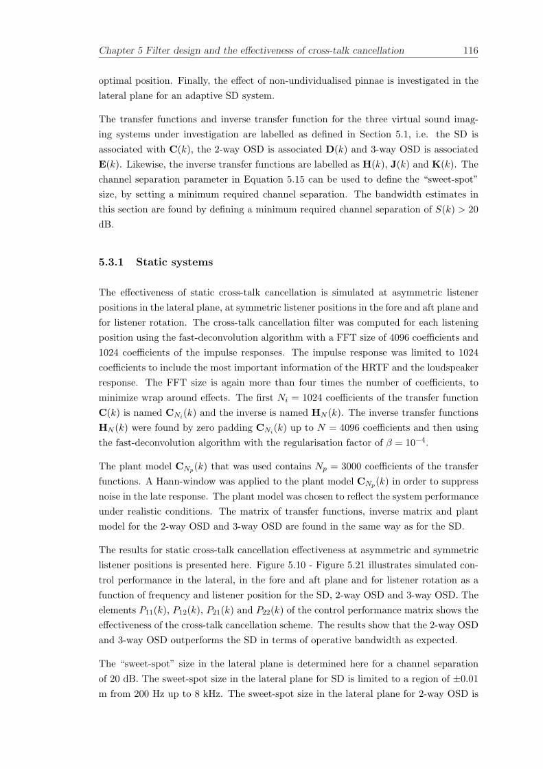
Chapter 5 Filter design and the effectiveness of cross-talk cancellation 116
optimal position. Finally, the effect of non-undividualised pinnae is investigated in thelateral plane for an adaptive SD system.
The transfer functions and inverse transfer function for the three virtual sound imag-ing systems under investigation are labelled as defined in Section 5.1, i.e. the SD isassociated with C(k), the 2-way OSD is associated D(k) and 3-way OSD is associatedE(k). Likewise, the inverse transfer functions are labelled as H(k), J(k) and K(k). Thechannel separation parameter in Equation 5.15 can be used to define the “sweet-spot”size, by setting a minimum required channel separation. The bandwidth estimates inthis section are found by defining a minimum required channel separation of S(k) > 20dB.
5.3.1 Static systems
The effectiveness of static cross-talk cancellation is simulated at asymmetric listenerpositions in the lateral plane, at symmetric listener positions in the fore and aft plane andfor listener rotation. The cross-talk cancellation filter was computed for each listeningposition using the fast-deconvolution algorithm with a FFT size of 4096 coefficients and1024 coefficients of the impulse responses. The impulse response was limited to 1024coefficients to include the most important information of the HRTF and the loudspeakerresponse. The FFT size is again more than four times the number of coefficients, tominimize wrap around effects. The first Ni = 1024 coefficients of the transfer functionC(k) is named CNi(k) and the inverse is named HN (k). The inverse transfer functionsHN (k) were found by zero padding CNi(k) up to N = 4096 coefficients and then usingthe fast-deconvolution algorithm with the regularisation factor of β = 10−4.
The plant model CNp(k) that was used contains Np = 3000 coefficients of the transferfunctions. A Hann-window was applied to the plant model CNp(k) in order to suppressnoise in the late response. The plant model was chosen to reflect the system performanceunder realistic conditions. The matrix of transfer functions, inverse matrix and plantmodel for the 2-way OSD and 3-way OSD are found in the same way as for the SD.
The results for static cross-talk cancellation effectiveness at asymmetric and symmetriclistener positions is presented here. Figure 5.10 - Figure 5.21 illustrates simulated con-trol performance in the lateral, in the fore and aft plane and for listener rotation as afunction of frequency and listener position for the SD, 2-way OSD and 3-way OSD. Theelements P11(k), P12(k), P21(k) and P22(k) of the control performance matrix shows theeffectiveness of the cross-talk cancellation scheme. The results show that the 2-way OSDand 3-way OSD outperforms the SD in terms of operative bandwidth as expected.
The “sweet-spot” size in the lateral plane is determined here for a channel separationof 20 dB. The sweet-spot size in the lateral plane for SD is limited to a region of ±0.01m from 200 Hz up to 8 kHz. The sweet-spot size in the lateral plane for 2-way OSD is
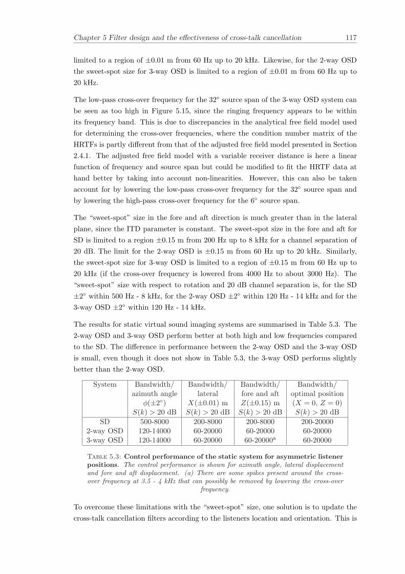
Chapter 5 Filter design and the effectiveness of cross-talk cancellation 117
limited to a region of ±0.01 m from 60 Hz up to 20 kHz. Likewise, for the 2-way OSDthe sweet-spot size for 3-way OSD is limited to a region of ±0.01 m from 60 Hz up to20 kHz.
The low-pass cross-over frequency for the 32 source span of the 3-way OSD system canbe seen as too high in Figure 5.15, since the ringing frequency appears to be withinits frequency band. This is due to discrepancies in the analytical free field model usedfor determining the cross-over frequencies, where the condition number matrix of theHRTFs is partly different from that of the adjusted free field model presented in Section2.4.1. The adjusted free field model with a variable receiver distance is here a linearfunction of frequency and source span but could be modified to fit the HRTF data athand better by taking into account non-linearities. However, this can also be takenaccount for by lowering the low-pass cross-over frequency for the 32 source span andby lowering the high-pass cross-over frequency for the 6 source span.
The “sweet-spot” size in the fore and aft direction is much greater than in the lateralplane, since the ITD parameter is constant. The sweet-spot size in the fore and aft forSD is limited to a region ±0.15 m from 200 Hz up to 8 kHz for a channel separation of20 dB. The limit for the 2-way OSD is ±0.15 m from 60 Hz up to 20 kHz. Similarly,the sweet-spot size for 3-way OSD is limited to a region of ±0.15 m from 60 Hz up to20 kHz (if the cross-over frequency is lowered from 4000 Hz to about 3000 Hz). The“sweet-spot” size with respect to rotation and 20 dB channel separation is, for the SD±2 within 500 Hz - 8 kHz, for the 2-way OSD ±2 within 120 Hz - 14 kHz and for the3-way OSD ±2 within 120 Hz - 14 kHz.
The results for static virtual sound imaging systems are summarised in Table 5.3. The2-way OSD and 3-way OSD perform better at both high and low frequencies comparedto the SD. The difference in performance between the 2-way OSD and the 3-way OSDis small, even though it does not show in Table 5.3, the 3-way OSD performs slightlybetter than the 2-way OSD.
System Bandwidth/ Bandwidth/ Bandwidth/ Bandwidth/azimuth angle lateral fore and aft optimal position
φ(±2) X(±0.01) m Z(±0.15) m (X = 0, Z = 0)S(k) > 20 dB S(k) > 20 dB S(k) > 20 dB S(k) > 20 dB
SD 500-8000 200-8000 200-8000 200-200002-way OSD 120-14000 60-20000 60-20000 60-200003-way OSD 120-14000 60-20000 60-20000a 60-20000
Table 5.3: Control performance of the static system for asymmetric listenerpositions. The control performance is shown for azimuth angle, lateral displacementand fore and aft displacement. (a) There are some spikes present around the cross-over frequency at 3.5 - 4 kHz that can possibly be removed by lowering the cross-over
frequency.
To overcome these limitations with the “sweet-spot” size, one solution is to update thecross-talk cancellation filters according to the listeners location and orientation. This is
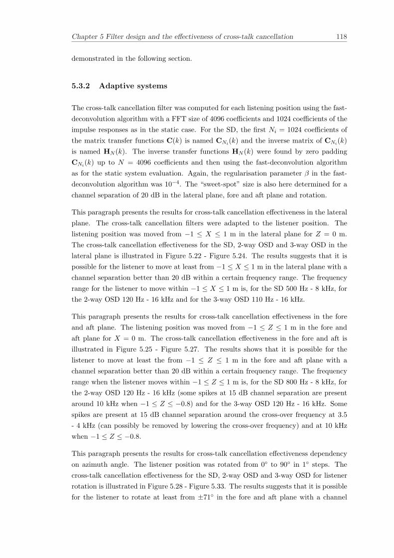
Chapter 5 Filter design and the effectiveness of cross-talk cancellation 118
demonstrated in the following section.
5.3.2 Adaptive systems
The cross-talk cancellation filter was computed for each listening position using the fast-deconvolution algorithm with a FFT size of 4096 coefficients and 1024 coefficients of theimpulse responses as in the static case. For the SD, the first Ni = 1024 coefficients ofthe matrix transfer functions C(k) is named CNi(k) and the inverse matrix of CNi(k)is named HN (k). The inverse transfer functions HN (k) were found by zero paddingCNi(k) up to N = 4096 coefficients and then using the fast-deconvolution algorithmas for the static system evaluation. Again, the regularisation parameter β in the fast-deconvolution algorithm was 10−4. The “sweet-spot” size is also here determined for achannel separation of 20 dB in the lateral plane, fore and aft plane and rotation.
This paragraph presents the results for cross-talk cancellation effectiveness in the lateralplane. The cross-talk cancellation filters were adapted to the listener position. Thelistening position was moved from −1 ≤ X ≤ 1 m in the lateral plane for Z = 0 m.The cross-talk cancellation effectiveness for the SD, 2-way OSD and 3-way OSD in thelateral plane is illustrated in Figure 5.22 - Figure 5.24. The results suggests that it ispossible for the listener to move at least from −1 ≤ X ≤ 1 m in the lateral plane with achannel separation better than 20 dB within a certain frequency range. The frequencyrange for the listener to move within −1 ≤ X ≤ 1 m is, for the SD 500 Hz - 8 kHz, forthe 2-way OSD 120 Hz - 16 kHz and for the 3-way OSD 110 Hz - 16 kHz.
This paragraph presents the results for cross-talk cancellation effectiveness in the foreand aft plane. The listening position was moved from −1 ≤ Z ≤ 1 m in the fore andaft plane for X = 0 m. The cross-talk cancellation effectiveness in the fore and aft isillustrated in Figure 5.25 - Figure 5.27. The results shows that it is possible for thelistener to move at least the from −1 ≤ Z ≤ 1 m in the fore and aft plane with achannel separation better than 20 dB within a certain frequency range. The frequencyrange when the listener moves within −1 ≤ Z ≤ 1 m is, for the SD 800 Hz - 8 kHz, forthe 2-way OSD 120 Hz - 16 kHz (some spikes at 15 dB channel separation are presentaround 10 kHz when −1 ≤ Z ≤ −0.8) and for the 3-way OSD 120 Hz - 16 kHz. Somespikes are present at 15 dB channel separation around the cross-over frequency at 3.5- 4 kHz (can possibly be removed by lowering the cross-over frequency) and at 10 kHzwhen −1 ≤ Z ≤ −0.8.
This paragraph presents the results for cross-talk cancellation effectiveness dependencyon azimuth angle. The listener position was rotated from 0 to 90 in 1 steps. Thecross-talk cancellation effectiveness for the SD, 2-way OSD and 3-way OSD for listenerrotation is illustrated in Figure 5.28 - Figure 5.33. The results suggests that it is possiblefor the listener to rotate at least from ±71 in the fore and aft plane with a channel
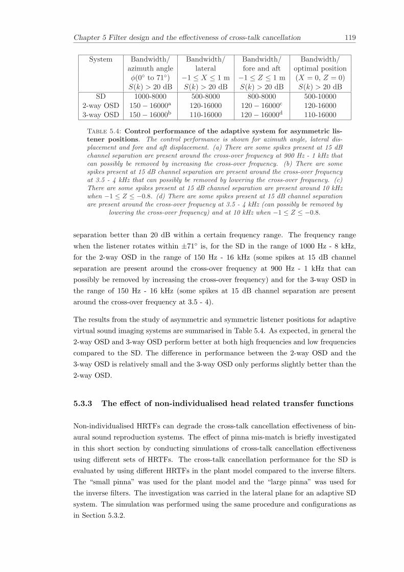
Chapter 5 Filter design and the effectiveness of cross-talk cancellation 119
System Bandwidth/ Bandwidth/ Bandwidth/ Bandwidth/azimuth angle lateral fore and aft optimal positionφ(0 to 71) −1 ≤ X ≤ 1 m −1 ≤ Z ≤ 1 m (X = 0, Z = 0)S(k) > 20 dB S(k) > 20 dB S(k) > 20 dB S(k) > 20 dB
SD 1000-8000 500-8000 800-8000 500-100002-way OSD 150− 16000a 120-16000 120− 16000c 120-160003-way OSD 150− 16000b 110-16000 120− 16000d 110-16000
Table 5.4: Control performance of the adaptive system for asymmetric lis-tener positions. The control performance is shown for azimuth angle, lateral dis-placement and fore and aft displacement. (a) There are some spikes present at 15 dBchannel separation are present around the cross-over frequency at 900 Hz - 1 kHz thatcan possibly be removed by increasing the cross-over frequency. (b) There are somespikes present at 15 dB channel separation are present around the cross-over frequencyat 3.5 - 4 kHz that can possibly be removed by lowering the cross-over frequency. (c)There are some spikes present at 15 dB channel separation are present around 10 kHzwhen −1 ≤ Z ≤ −0.8. (d) There are some spikes present at 15 dB channel separationare present around the cross-over frequency at 3.5 - 4 kHz (can possibly be removed by
lowering the cross-over frequency) and at 10 kHz when −1 ≤ Z ≤ −0.8.
separation better than 20 dB within a certain frequency range. The frequency rangewhen the listener rotates within ±71 is, for the SD in the range of 1000 Hz - 8 kHz,for the 2-way OSD in the range of 150 Hz - 16 kHz (some spikes at 15 dB channelseparation are present around the cross-over frequency at 900 Hz - 1 kHz that canpossibly be removed by increasing the cross-over frequency) and for the 3-way OSD inthe range of 150 Hz - 16 kHz (some spikes at 15 dB channel separation are presentaround the cross-over frequency at 3.5 - 4).
The results from the study of asymmetric and symmetric listener positions for adaptivevirtual sound imaging systems are summarised in Table 5.4. As expected, in general the2-way OSD and 3-way OSD perform better at both high frequencies and low frequenciescompared to the SD. The difference in performance between the 2-way OSD and the3-way OSD is relatively small and the 3-way OSD only performs slightly better than the2-way OSD.
5.3.3 The effect of non-individualised head related transfer functions
Non-individualised HRTFs can degrade the cross-talk cancellation effectiveness of bin-aural sound reproduction systems. The effect of pinna mis-match is briefly investigatedin this short section by conducting simulations of cross-talk cancellation effectivenessusing different sets of HRTFs. The cross-talk cancellation performance for the SD isevaluated by using different HRTFs in the plant model compared to the inverse filters.The “small pinna” was used for the plant model and the “large pinna” was used forthe inverse filters. The investigation was carried in the lateral plane for an adaptive SDsystem. The simulation was performed using the same procedure and configurations asin Section 5.3.2.
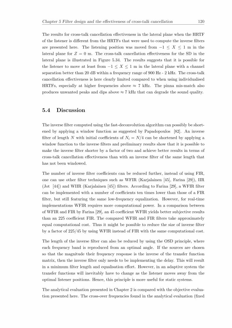
Chapter 5 Filter design and the effectiveness of cross-talk cancellation 120
The results for cross-talk cancellation effectiveness in the lateral plane when the HRTFof the listener is different from the HRTFs that were used to compute the inverse filtersare presented here. The listening position was moved from −1 ≤ X ≤ 1 m in thelateral plane for Z = 0 m. The cross-talk cancellation effectiveness for the SD in thelateral plane is illustrated in Figure 5.34. The results suggests that it is possible forthe listener to move at least from −1 ≤ X ≤ 1 m in the lateral plane with a channelseparation better than 20 dB within a frequency range of 900 Hz - 2 kHz. The cross-talkcancellation effectiveness is here clearly limited compared to when using individualisedHRTFs, especially at higher frequencies above ≈ 7 kHz. The pinna mis-match alsoproduces unwanted peaks and dips above ≈ 7 kHz that can degrade the sound quality.
5.4 Discussion
The inverse filter computed using the fast-deconvolution algorithm can possibly be short-ened by applying a window function as suggested by Papadopoulos [82]. An inversefilter of length N with initial coefficients of Ni = N/4 can be shortened by applying awindow function to the inverse filters and preliminary results show that it is possible tomake the inverse filter shorter by a factor of two and achieve better results in terms ofcross-talk cancellation effectiveness than with an inverse filter of the same length thathas not been windowed.
The number of inverse filter coefficients can be reduced further, instead of using FIR,one can use other filter techniques such as WFIR (Karjalainen [45], Farina [29]), IIR(Jot [44]) and WIIR (Karjalainen [45]) filters. According to Farina [29], a WFIR filtercan be implemented with a number of coefficients ten times lower than those of a FIRfilter, but still featuring the same low-frequency equalization. However, for real-timeimplementations WFIR requires more computational power. In a comparison betweenof WFIR and FIR by Farina [29], an 45 coefficient WFIR yields better subjective resultsthan an 225 coefficient FIR. The compared WFIR and FIR filters take approximatelyequal computational cost. Thus it might be possible to reduce the size of inverse filterby a factor of 225/45 by using WFIR instead of FIR with the same computational cost.
The length of the inverse filter can also be reduced by using the OSD principle, whereeach frequency band is reproduced from an optimal angle. If the sources are chosenso that the magnitude their frequency response is the inverse of the transfer functionmatrix, then the inverse filter only needs to be implementing the delay. This will resultin a minimum filter length and equalisation effort. However, in an adaptive system thetransfer functions will inevitably have to change as the listener moves away from theoptimal listener positions. Hence, this principle is more useful for static systems.
The analytical evaluation presented in Chapter 2 is compared with the objective evalua-tion presented here. The cross-over frequencies found in the analytical evaluation (fixed
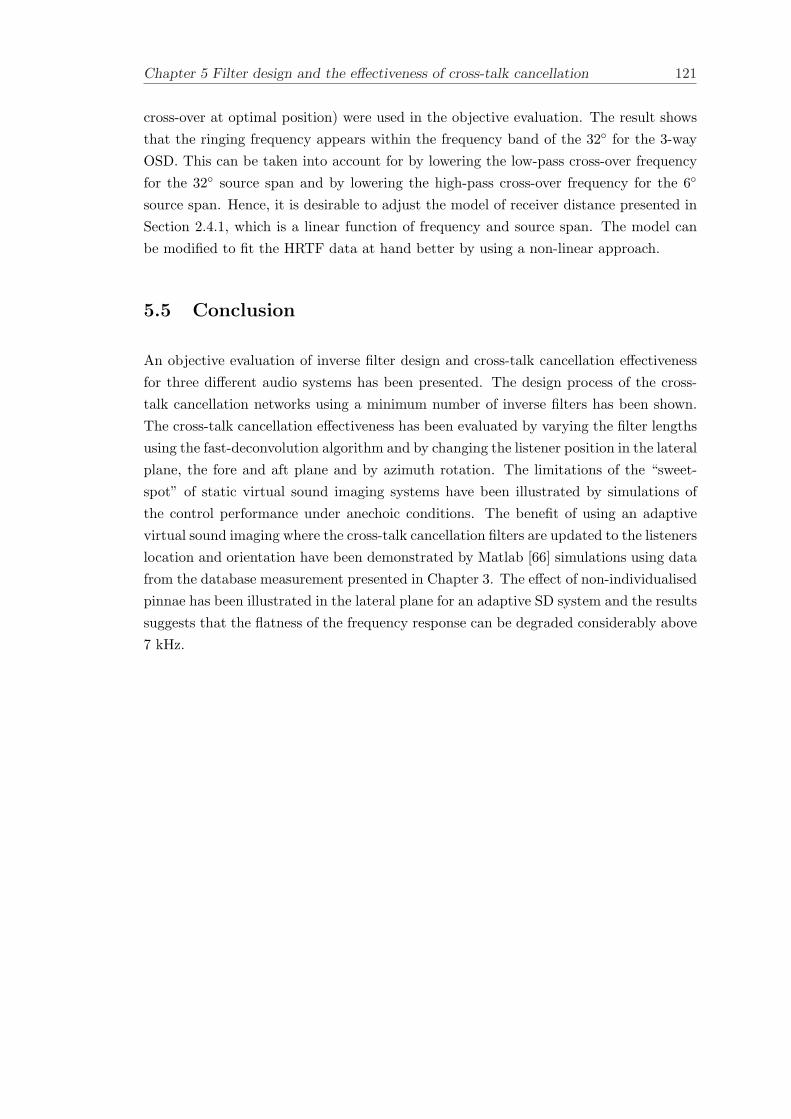
Chapter 5 Filter design and the effectiveness of cross-talk cancellation 121
cross-over at optimal position) were used in the objective evaluation. The result showsthat the ringing frequency appears within the frequency band of the 32 for the 3-wayOSD. This can be taken into account for by lowering the low-pass cross-over frequencyfor the 32 source span and by lowering the high-pass cross-over frequency for the 6
source span. Hence, it is desirable to adjust the model of receiver distance presented inSection 2.4.1, which is a linear function of frequency and source span. The model canbe modified to fit the HRTF data at hand better by using a non-linear approach.
5.5 Conclusion
An objective evaluation of inverse filter design and cross-talk cancellation effectivenessfor three different audio systems has been presented. The design process of the cross-talk cancellation networks using a minimum number of inverse filters has been shown.The cross-talk cancellation effectiveness has been evaluated by varying the filter lengthsusing the fast-deconvolution algorithm and by changing the listener position in the lateralplane, the fore and aft plane and by azimuth rotation. The limitations of the “sweet-spot” of static virtual sound imaging systems have been illustrated by simulations ofthe control performance under anechoic conditions. The benefit of using an adaptivevirtual sound imaging where the cross-talk cancellation filters are updated to the listenerslocation and orientation have been demonstrated by Matlab [66] simulations using datafrom the database measurement presented in Chapter 3. The effect of non-individualisedpinnae has been illustrated in the lateral plane for an adaptive SD system and the resultssuggests that the flatness of the frequency response can be degraded considerably above7 kHz.
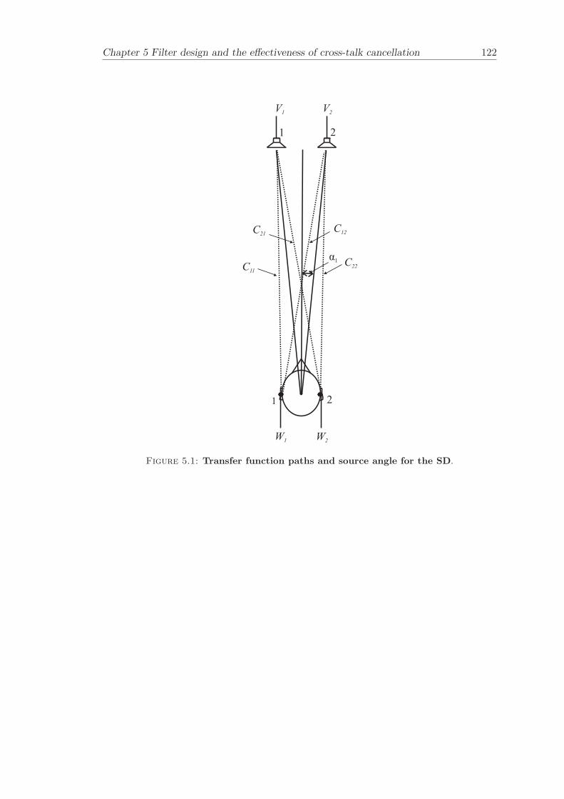
Chapter 5 Filter design and the effectiveness of cross-talk cancellation 122
C11
C21
C12
C22
1 2
1 2
W1
W2
V1
V2
α1
Figure 5.1: Transfer function paths and source angle for the SD.
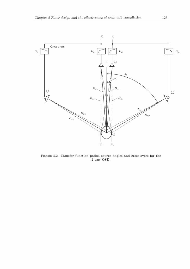
Chapter 5 Filter design and the effectiveness of cross-talk cancellation 123
D11,2
D21,2
D11,1
D12,1D21,1
D22,1
1,2
1,1 2,1
2,2
V1 V2
Cross overs
D21,2
D22,2
1 2
W1 W2
σ1
σ2
G12 G11 G21 G22
Figure 5.2: Transfer function paths, source angles and cross-overs for the2-way OSD.
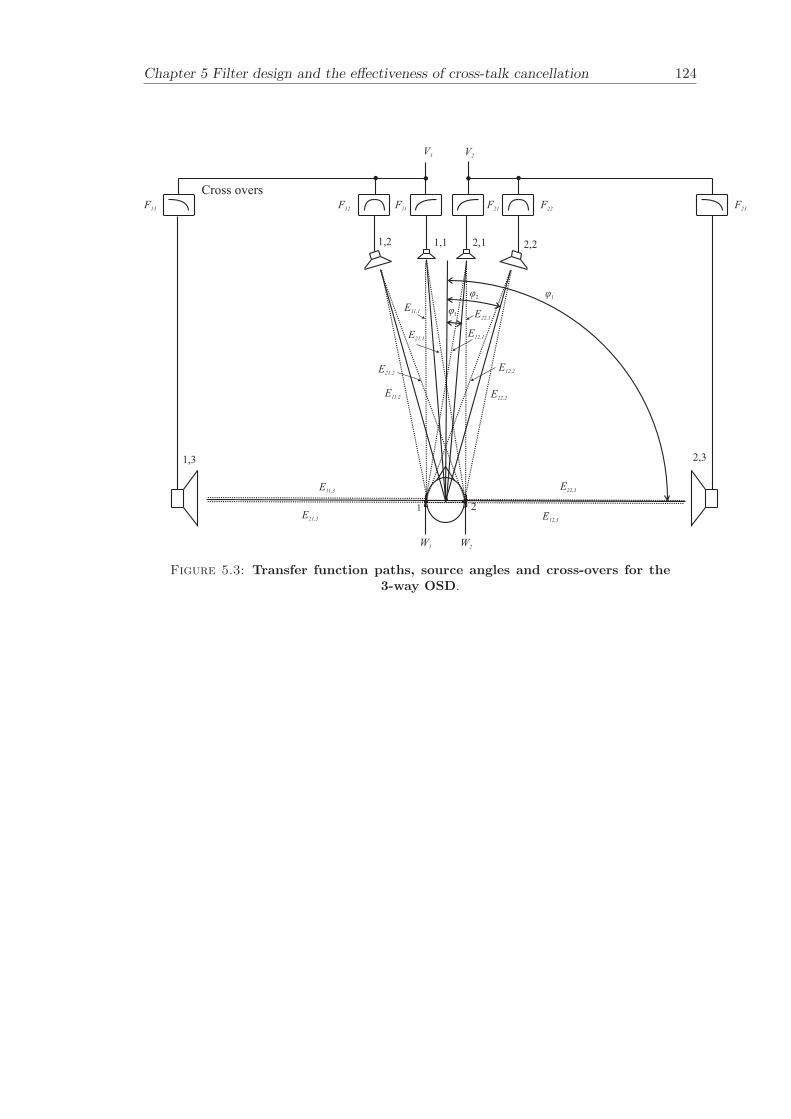
Chapter 5 Filter design and the effectiveness of cross-talk cancellation 124
E11,3
E21,3
E11,2
E21,2
E11,1
E21,1E12,1
E22,1
E12,2
E22,2
V1 V2
Cross overs
1,3
E22,3
E12,3
2,3
1,2 1,1 2,1 2,2
1 2
W1 W2
φ2
φ1
φ1
F13 F12 F11 F21 F22 F23
Figure 5.3: Transfer function paths, source angles and cross-overs for the3-way OSD.
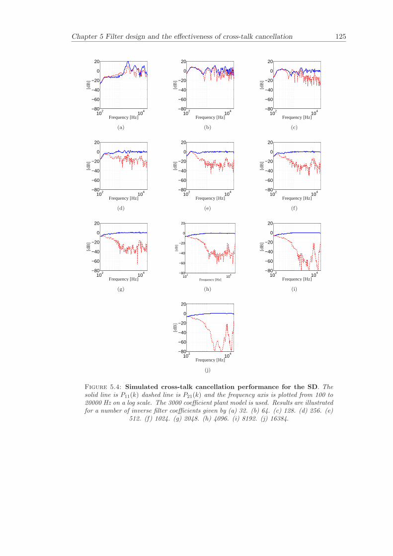
Chapter 5 Filter design and the effectiveness of cross-talk cancellation 125
102
104−80
−60
−40
−20
0
20
Frequency [Hz]
[dB
]
(a)
102
104−80
−60
−40
−20
0
20
Frequency [Hz]
[dB
]
(b)
102
104−80
−60
−40
−20
0
20
Frequency [Hz]
[dB
]
(c)
102
104−80
−60
−40
−20
0
20
Frequency [Hz]
[dB
]
(d)
102
104−80
−60
−40
−20
0
20
Frequency [Hz]
[dB
]
(e)
102
104−80
−60
−40
−20
0
20
Frequency [Hz]
[dB
]
(f)
102
104−80
−60
−40
−20
0
20
Frequency [Hz]
[dB
]
(g)
102
104−80
−60
−40
−20
0
20
Frequency [Hz]
[dB
]
(h)
102
104−80
−60
−40
−20
0
20
Frequency [Hz]
[dB
]
(i)
102
104−80
−60
−40
−20
0
20
Frequency [Hz]
[dB
]
(j)
Figure 5.4: Simulated cross-talk cancellation performance for the SD. Thesolid line is P11(k) dashed line is P21(k) and the frequency axis is plotted from 100 to20000 Hz on a log scale. The 3000 coefficient plant model is used. Results are illustratedfor a number of inverse filter coefficients given by (a) 32. (b) 64. (c) 128. (d) 256. (e)
512. (f) 1024. (g) 2048. (h) 4096. (i) 8192. (j) 16384.
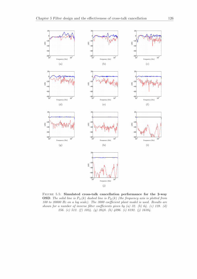
Chapter 5 Filter design and the effectiveness of cross-talk cancellation 126
102
104−80
−60
−40
−20
0
20
Frequency [Hz]
[dB
]
(a)
102
104−80
−60
−40
−20
0
20
Frequency [Hz]
[dB
]
(b)
102
104−80
−60
−40
−20
0
20
Frequency [Hz]
[dB
]
(c)
102
104−80
−60
−40
−20
0
20
Frequency [Hz]
[dB
]
(d)
102
104−80
−60
−40
−20
0
20
Frequency [Hz]
[dB
]
(e)
102
104−80
−60
−40
−20
0
20
Frequency [Hz]
[dB
]
(f)
102
104−80
−60
−40
−20
0
20
Frequency [Hz]
[dB
]
(g)
102
104−80
−60
−40
−20
0
20
Frequency [Hz]
[dB
]
(h)
102
104−80
−60
−40
−20
0
20
Frequency [Hz]
[dB
]
(i)
102
104−80
−60
−40
−20
0
20
Frequency [Hz]
[dB
]
(j)
Figure 5.5: Simulated cross-talk cancellation performance for the 2-wayOSD. The solid line is P11(k) dashed line is P21(k) (the frequency axis is plotted from100 to 20000 Hz on a log scale). The 3000 coefficient plant model is used. Results areshown for a number of inverse filter coefficients given by (a) 32. (b) 64. (c) 128. (d)
256. (e) 512. (f) 1024. (g) 2048. (h) 4096. (i) 8192. (j) 16384.
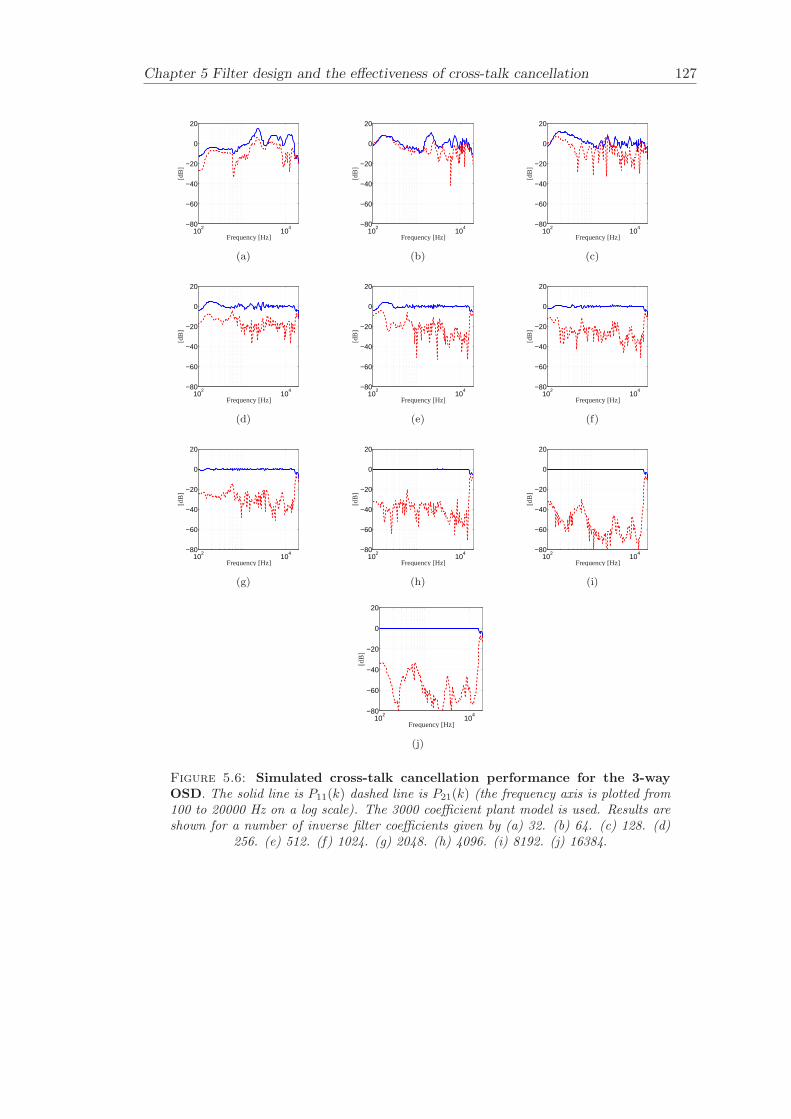
Chapter 5 Filter design and the effectiveness of cross-talk cancellation 127
102
104−80
−60
−40
−20
0
20
Frequency [Hz]
[dB
]
(a)
102
104−80
−60
−40
−20
0
20
Frequency [Hz]
[dB
]
(b)
102
104−80
−60
−40
−20
0
20
Frequency [Hz]
[dB
]
(c)
102
104−80
−60
−40
−20
0
20
Frequency [Hz]
[dB
]
(d)
102
104−80
−60
−40
−20
0
20
Frequency [Hz]
[dB
]
(e)
102
104−80
−60
−40
−20
0
20
Frequency [Hz]
[dB
]
(f)
102
104−80
−60
−40
−20
0
20
Frequency [Hz]
[dB
]
(g)
102
104−80
−60
−40
−20
0
20
Frequency [Hz]
[dB
]
(h)
102
104−80
−60
−40
−20
0
20
Frequency [Hz]
[dB
]
(i)
102
104−80
−60
−40
−20
0
20
Frequency [Hz]
[dB
]
(j)
Figure 5.6: Simulated cross-talk cancellation performance for the 3-wayOSD. The solid line is P11(k) dashed line is P21(k) (the frequency axis is plotted from100 to 20000 Hz on a log scale). The 3000 coefficient plant model is used. Results areshown for a number of inverse filter coefficients given by (a) 32. (b) 64. (c) 128. (d)
256. (e) 512. (f) 1024. (g) 2048. (h) 4096. (i) 8192. (j) 16384.
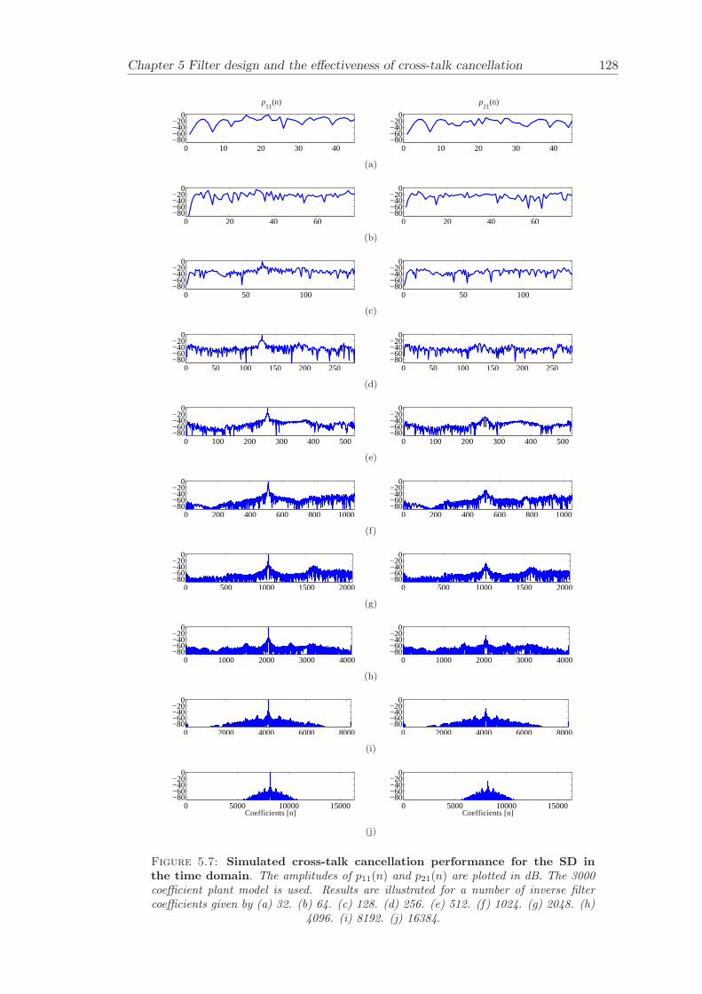
Chapter 5 Filter design and the effectiveness of cross-talk cancellation 128
0 10 20 30 40−80−60−40−20
0
p11
(n)
0 10 20 30 40−80−60−40−20
0
p21
(n)
(a)
0 20 40 60−80−60−40−20
0
0 20 40 60−80−60−40−20
0
(b)
0 50 100−80−60−40−20
0
0 50 100−80−60−40−20
0
(c)
0 50 100 150 200 250−80−60−40−20
0
0 50 100 150 200 250−80−60−40−20
0
(d)
0 100 200 300 400 500−80−60−40−20
0
0 100 200 300 400 500−80−60−40−20
0
(e)
0 200 400 600 800 1000−80−60−40−20
0
0 200 400 600 800 1000−80−60−40−20
0
(f)
0 500 1000 1500 2000−80−60−40−20
0
0 500 1000 1500 2000−80−60−40−20
0
(g)
0 1000 2000 3000 4000−80−60−40−20
0
0 1000 2000 3000 4000−80−60−40−20
0
(h)
0 2000 4000 6000 8000−80−60−40−20
0
0 2000 4000 6000 8000−80−60−40−20
0
(i)
0 5000 10000 15000−80−60−40−20
0
Coefficients [n]0 5000 10000 15000
−80−60−40−20
0
Coefficients [n]
(j)
Figure 5.7: Simulated cross-talk cancellation performance for the SD inthe time domain. The amplitudes of p11(n) and p21(n) are plotted in dB. The 3000coefficient plant model is used. Results are illustrated for a number of inverse filtercoefficients given by (a) 32. (b) 64. (c) 128. (d) 256. (e) 512. (f) 1024. (g) 2048. (h)
4096. (i) 8192. (j) 16384.
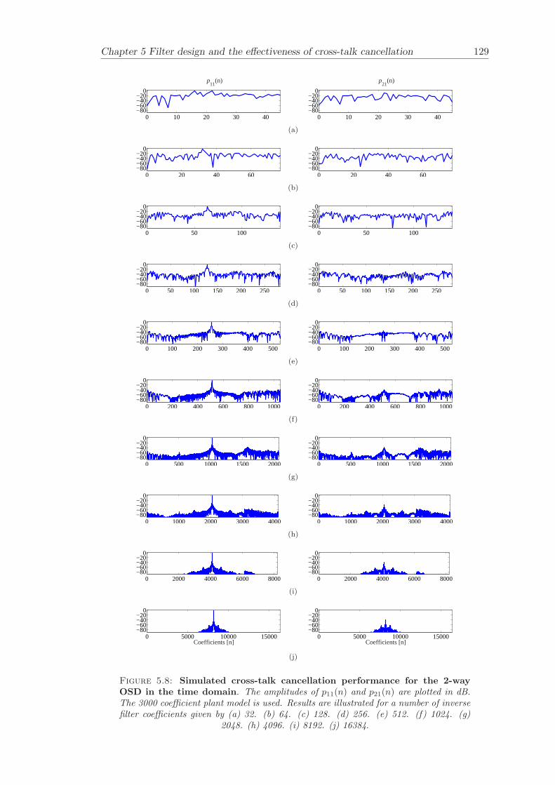
Chapter 5 Filter design and the effectiveness of cross-talk cancellation 129
0 10 20 30 40−80−60−40−20
0
p11
(n)
0 10 20 30 40−80−60−40−20
0
p21
(n)
(a)
0 20 40 60−80−60−40−20
0
0 20 40 60−80−60−40−20
0
(b)
0 50 100−80−60−40−20
0
0 50 100−80−60−40−20
0
(c)
0 50 100 150 200 250−80−60−40−20
0
0 50 100 150 200 250−80−60−40−20
0
(d)
0 100 200 300 400 500−80−60−40−20
0
0 100 200 300 400 500−80−60−40−20
0
(e)
0 200 400 600 800 1000−80−60−40−20
0
0 200 400 600 800 1000−80−60−40−20
0
(f)
0 500 1000 1500 2000−80−60−40−20
0
0 500 1000 1500 2000−80−60−40−20
0
(g)
0 1000 2000 3000 4000−80−60−40−20
0
0 1000 2000 3000 4000−80−60−40−20
0
(h)
0 2000 4000 6000 8000−80−60−40−20
0
0 2000 4000 6000 8000−80−60−40−20
0
(i)
0 5000 10000 15000−80−60−40−20
0
Coefficients [n]0 5000 10000 15000
−80−60−40−20
0
Coefficients [n]
(j)
Figure 5.8: Simulated cross-talk cancellation performance for the 2-wayOSD in the time domain. The amplitudes of p11(n) and p21(n) are plotted in dB.The 3000 coefficient plant model is used. Results are illustrated for a number of inversefilter coefficients given by (a) 32. (b) 64. (c) 128. (d) 256. (e) 512. (f) 1024. (g)
2048. (h) 4096. (i) 8192. (j) 16384.
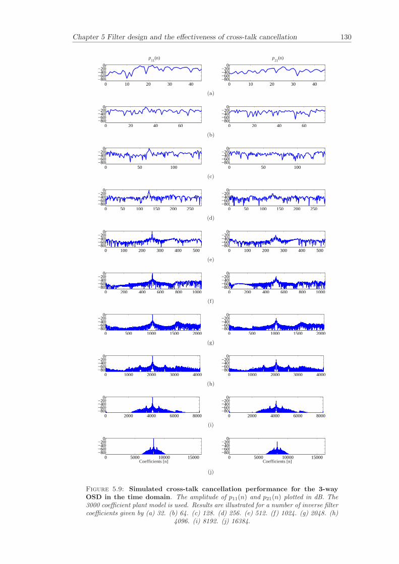
Chapter 5 Filter design and the effectiveness of cross-talk cancellation 130
0 10 20 30 40−80−60−40−20
0
p11
(n)
0 10 20 30 40−80−60−40−20
0
p21
(n)
(a)
0 20 40 60−80−60−40−20
0
0 20 40 60−80−60−40−20
0
(b)
0 50 100−80−60−40−20
0
0 50 100−80−60−40−20
0
(c)
0 50 100 150 200 250−80−60−40−20
0
0 50 100 150 200 250−80−60−40−20
0
(d)
0 100 200 300 400 500−80−60−40−20
0
0 100 200 300 400 500−80−60−40−20
0
(e)
0 200 400 600 800 1000−80−60−40−20
0
0 200 400 600 800 1000−80−60−40−20
0
(f)
0 500 1000 1500 2000−80−60−40−20
0
0 500 1000 1500 2000−80−60−40−20
0
(g)
0 1000 2000 3000 4000−80−60−40−20
0
0 1000 2000 3000 4000−80−60−40−20
0
(h)
0 2000 4000 6000 8000−80−60−40−20
0
0 2000 4000 6000 8000−80−60−40−20
0
(i)
0 5000 10000 15000−80−60−40−20
0
Coefficients [n]0 5000 10000 15000
−80−60−40−20
0
Coefficients [n]
(j)
Figure 5.9: Simulated cross-talk cancellation performance for the 3-wayOSD in the time domain. The amplitude of p11(n) and p21(n) plotted in dB. The3000 coefficient plant model is used. Results are illustrated for a number of inverse filtercoefficients given by (a) 32. (b) 64. (c) 128. (d) 256. (e) 512. (f) 1024. (g) 2048. (h)
4096. (i) 8192. (j) 16384.
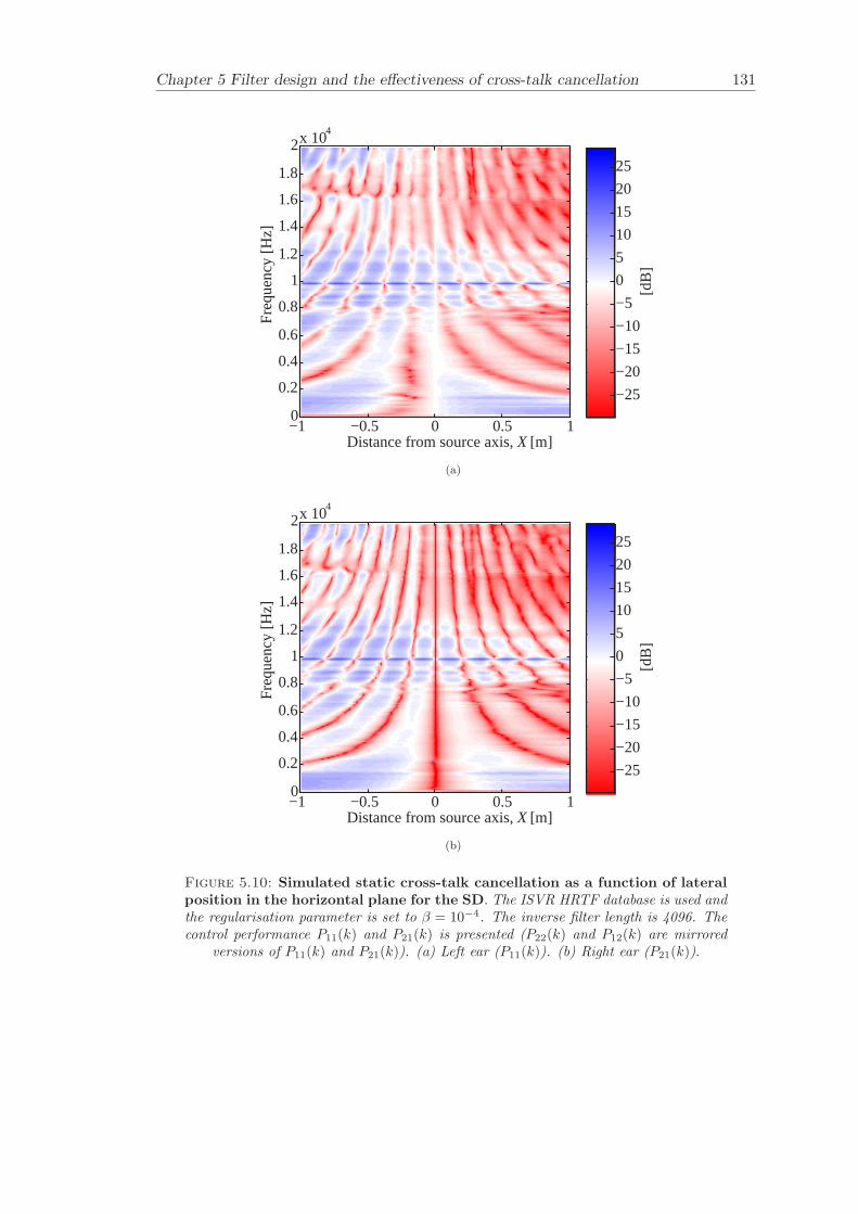
Chapter 5 Filter design and the effectiveness of cross-talk cancellation 131
Distance from source axis, X [m]
Fre
quen
cy [H
z]
−1 −0.5 0 0.5 10
0.2
0.4
0.6
0.8
1
1.2
1.4
1.6
1.8
2x 10⁴
[dB
]
−25
−20
−15
−10
−5
0
5
10
15
20
25
(a)
Distance from source axis, X [m]
Fre
quen
cy [H
z]
−1 −0.5 0 0.5 10
0.2
0.4
0.6
0.8
1
1.2
1.4
1.6
1.8
2x 10⁴
[dB
]
−25
−20
−15
−10
−5
0
5
10
15
20
25
(b)
Figure 5.10: Simulated static cross-talk cancellation as a function of lateralposition in the horizontal plane for the SD. The ISVR HRTF database is used andthe regularisation parameter is set to β = 10−4. The inverse filter length is 4096. Thecontrol performance P11(k) and P21(k) is presented (P22(k) and P12(k) are mirrored
versions of P11(k) and P21(k)). (a) Left ear (P11(k)). (b) Right ear (P21(k)).
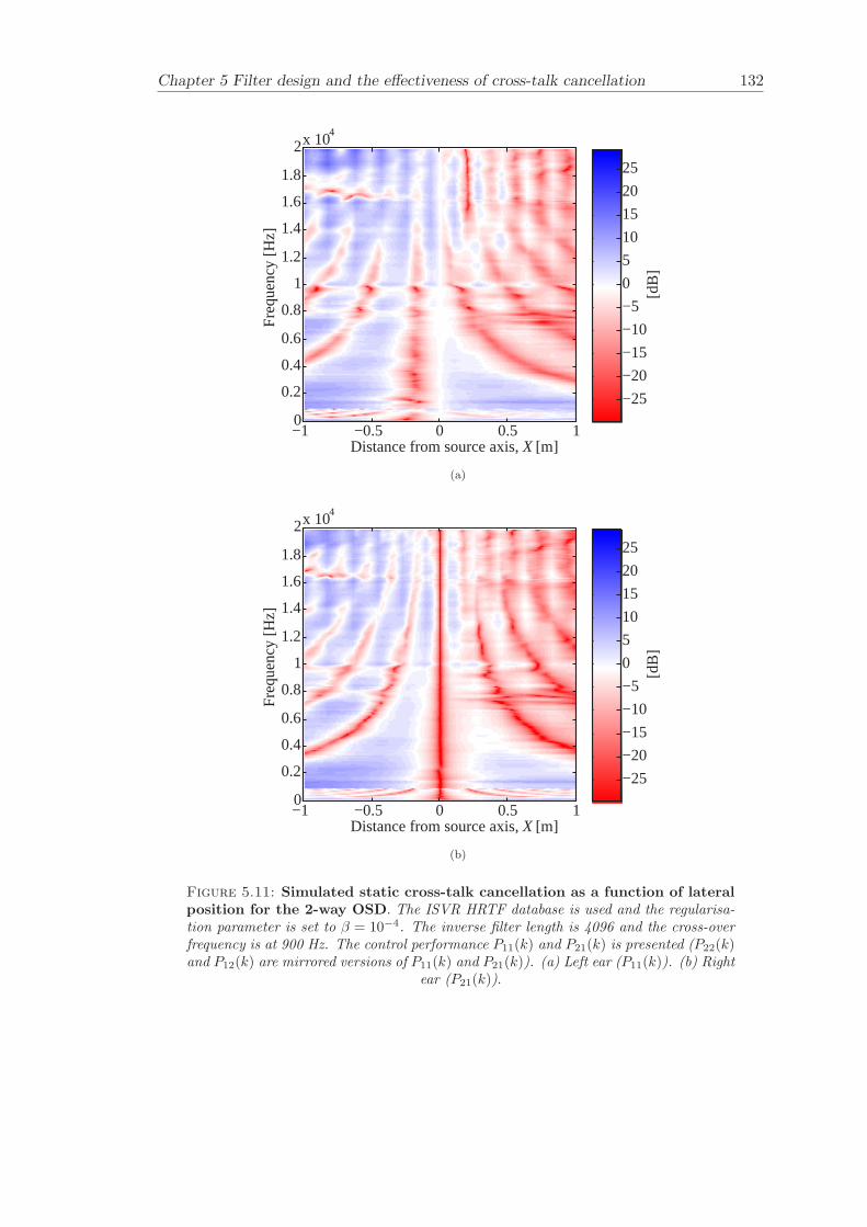
Chapter 5 Filter design and the effectiveness of cross-talk cancellation 132
Distance from source axis, X [m]
Fre
quen
cy [H
z]
−1 −0.5 0 0.5 10
0.2
0.4
0.6
0.8
1
1.2
1.4
1.6
1.8
2x 10⁴
[dB
]
−25
−20
−15
−10
−5
0
5
10
15
20
25
(a)
Distance from source axis, X [m]
Fre
quen
cy [H
z]
−1 −0.5 0 0.5 10
0.2
0.4
0.6
0.8
1
1.2
1.4
1.6
1.8
2x 10⁴
[dB
]
−25
−20
−15
−10
−5
0
5
10
15
20
25
(b)
Figure 5.11: Simulated static cross-talk cancellation as a function of lateralposition for the 2-way OSD. The ISVR HRTF database is used and the regularisa-tion parameter is set to β = 10−4. The inverse filter length is 4096 and the cross-overfrequency is at 900 Hz. The control performance P11(k) and P21(k) is presented (P22(k)and P12(k) are mirrored versions of P11(k) and P21(k)). (a) Left ear (P11(k)). (b) Right
ear (P21(k)).
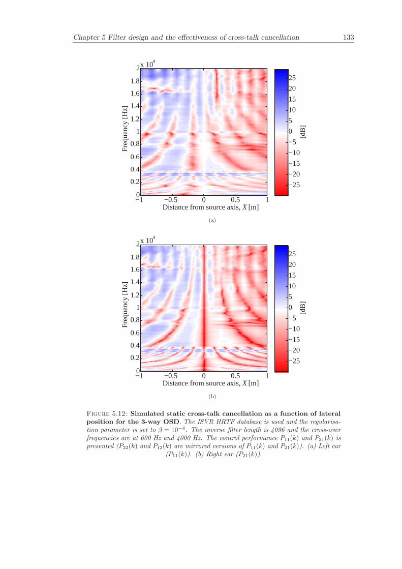
Chapter 5 Filter design and the effectiveness of cross-talk cancellation 133
Distance from source axis, X [m]
Fre
quen
cy [H
z]
−1 −0.5 0 0.5 10
0.2
0.4
0.6
0.8
1
1.2
1.4
1.6
1.8
2x 10⁴
[dB
]
−25
−20
−15
−10
−5
0
5
10
15
20
25
(a)
Distance from source axis, X [m]
Fre
quen
cy [H
z]
−1 −0.5 0 0.5 10
0.2
0.4
0.6
0.8
1
1.2
1.4
1.6
1.8
2x 10⁴
[dB
]
−25
−20
−15
−10
−5
0
5
10
15
20
25
(b)
Figure 5.12: Simulated static cross-talk cancellation as a function of lateralposition for the 3-way OSD. The ISVR HRTF database is used and the regularisa-tion parameter is set to β = 10−4. The inverse filter length is 4096 and the cross-overfrequencies are at 600 Hz and 4000 Hz. The control performance P11(k) and P21(k) ispresented (P22(k) and P12(k) are mirrored versions of P11(k) and P21(k)). (a) Left ear
(P11(k)). (b) Right ear (P21(k)).
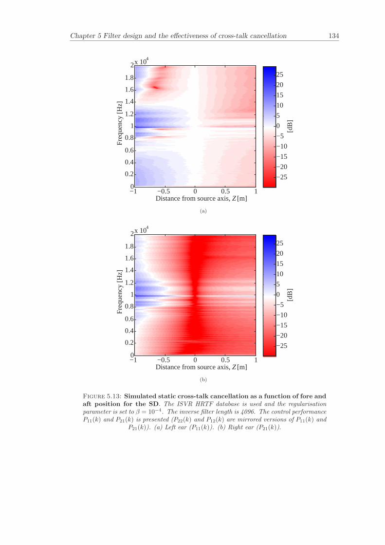
Chapter 5 Filter design and the effectiveness of cross-talk cancellation 134
Distance from source axis, Z [m]
Fre
quen
cy [H
z]
−1 −0.5 0 0.5 10
0.2
0.4
0.6
0.8
1
1.2
1.4
1.6
1.8
2x 10⁴
[dB
]
−25
−20
−15
−10
−5
0
5
10
15
20
25
(a)
Distance from source axis, Z [m]
Fre
quen
cy [H
z]
−1 −0.5 0 0.5 10
0.2
0.4
0.6
0.8
1
1.2
1.4
1.6
1.8
2x 10⁴
[dB
]
−25
−20
−15
−10
−5
0
5
10
15
20
25
(b)
Figure 5.13: Simulated static cross-talk cancellation as a function of fore andaft position for the SD. The ISVR HRTF database is used and the regularisationparameter is set to β = 10−4. The inverse filter length is 4096. The control performanceP11(k) and P21(k) is presented (P22(k) and P12(k) are mirrored versions of P11(k) and
P21(k)). (a) Left ear (P11(k)). (b) Right ear (P21(k)).
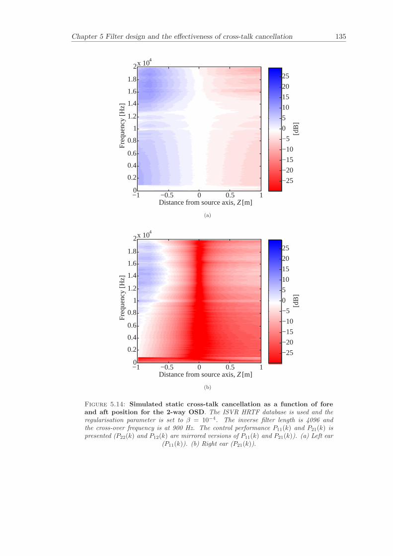
Chapter 5 Filter design and the effectiveness of cross-talk cancellation 135
Distance from source axis, Z [m]
Fre
quen
cy [H
z]
−1 −0.5 0 0.5 10
0.2
0.4
0.6
0.8
1
1.2
1.4
1.6
1.8
2x 10⁴
[dB
]
−25
−20
−15
−10
−5
0
5
10
15
20
25
(a)
Distance from source axis, Z [m]
Fre
quen
cy [H
z]
−1 −0.5 0 0.5 10
0.2
0.4
0.6
0.8
1
1.2
1.4
1.6
1.8
2x 10⁴
[dB
]
−25
−20
−15
−10
−5
0
5
10
15
20
25
(b)
Figure 5.14: Simulated static cross-talk cancellation as a function of foreand aft position for the 2-way OSD. The ISVR HRTF database is used and theregularisation parameter is set to β = 10−4. The inverse filter length is 4096 andthe cross-over frequency is at 900 Hz. The control performance P11(k) and P21(k) ispresented (P22(k) and P12(k) are mirrored versions of P11(k) and P21(k)). (a) Left ear
(P11(k)). (b) Right ear (P21(k)).
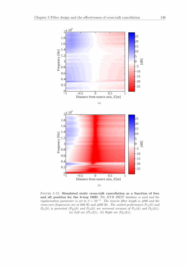
Chapter 5 Filter design and the effectiveness of cross-talk cancellation 136
Distance from source axis, Z [m]
Fre
quen
cy [H
z]
−1 −0.5 0 0.5 10
0.2
0.4
0.6
0.8
1
1.2
1.4
1.6
1.8
2x 10⁴
[dB
]
−25
−20
−15
−10
−5
0
5
10
15
20
25
(a)
Distance from source axis, Z [m]
Fre
quen
cy [H
z]
−1 −0.5 0 0.5 10
0.2
0.4
0.6
0.8
1
1.2
1.4
1.6
1.8
2x 10⁴
[dB
]
−25
−20
−15
−10
−5
0
5
10
15
20
25
(b)
Figure 5.15: Simulated static cross-talk cancellation as a function of foreand aft position for the 3-way OSD. The ISVR HRTF database is used and theregularisation parameter is set to β = 10−4. The inverse filter length is 4096 and thecross-over frequencies are at 600 Hz and 4000 Hz. The control performance P11(k) andP21(k) is presented (P22(k) and P12(k) are mirrored versions of P11(k) and P21(k)).
(a) Left ear (P11(k)). (b) Right ear (P21(k)).
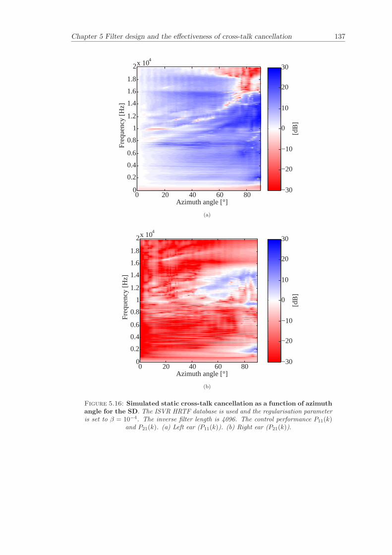
Chapter 5 Filter design and the effectiveness of cross-talk cancellation 137
Fre
quen
cy [H
z]
Azimuth angle [°]0 20 40 60 80
0
0.2
0.4
0.6
0.8
1
1.2
1.4
1.6
1.8
2x 10⁴
[dB
]
−30
−20
−10
0
10
20
30
(a)
Fre
quen
cy [H
z]
Azimuth angle [°]0 20 40 60 80
0
0.2
0.4
0.6
0.8
1
1.2
1.4
1.6
1.8
2x 10⁴
[dB
]
−30
−20
−10
0
10
20
30
(b)
Figure 5.16: Simulated static cross-talk cancellation as a function of azimuthangle for the SD. The ISVR HRTF database is used and the regularisation parameteris set to β = 10−4. The inverse filter length is 4096. The control performance P11(k)
and P21(k). (a) Left ear (P11(k)). (b) Right ear (P21(k)).
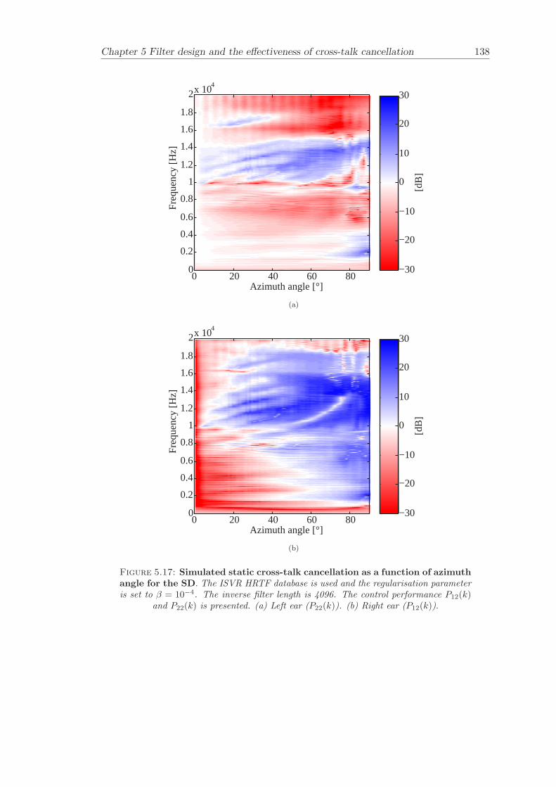
Chapter 5 Filter design and the effectiveness of cross-talk cancellation 138
Fre
quen
cy [H
z]
Azimuth angle [°]0 20 40 60 80
0
0.2
0.4
0.6
0.8
1
1.2
1.4
1.6
1.8
2x 10⁴
[dB
]
−30
−20
−10
0
10
20
30
(a)
Fre
quen
cy [H
z]
Azimuth angle [°]0 20 40 60 80
0
0.2
0.4
0.6
0.8
1
1.2
1.4
1.6
1.8
2x 10⁴
[dB
]
−30
−20
−10
0
10
20
30
(b)
Figure 5.17: Simulated static cross-talk cancellation as a function of azimuthangle for the SD. The ISVR HRTF database is used and the regularisation parameteris set to β = 10−4. The inverse filter length is 4096. The control performance P12(k)
and P22(k) is presented. (a) Left ear (P22(k)). (b) Right ear (P12(k)).

Chapter 5 Filter design and the effectiveness of cross-talk cancellation 139
Fre
quen
cy [H
z]
Azimuth angle [°]0 20 40 60 80
0
0.2
0.4
0.6
0.8
1
1.2
1.4
1.6
1.8
2x 10⁴
[dB
]
−30
−20
−10
0
10
20
30
(a)
Fre
quen
cy [H
z]
Azimuth angle [°]0 20 40 60 80
0
0.2
0.4
0.6
0.8
1
1.2
1.4
1.6
1.8
2x 10⁴
[dB
]
−30
−20
−10
0
10
20
30
(b)
Figure 5.18: Simulated static cross-talk cancellation as a function of azimuthangle for the 2-way OSD. The ISVR HRTF database is used and the regularisationparameter is set to β = 10−4. The inverse filter length is 4096 and the cross-overfrequencies is at 900 Hz. The control performance P11(k) and P21(k) is presented. (a)
Left ear (P11(k)). (b) Right ear (P21(k)).
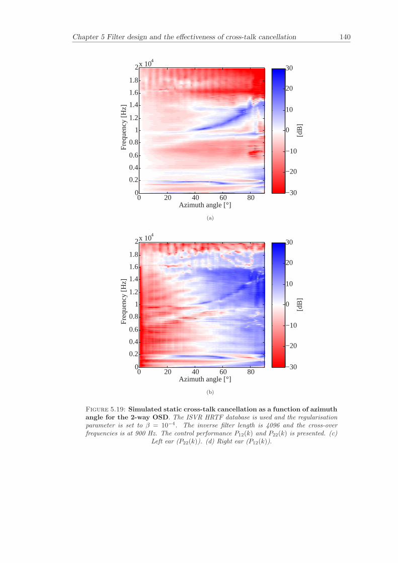
Chapter 5 Filter design and the effectiveness of cross-talk cancellation 140
Fre
quen
cy [H
z]
Azimuth angle [°]0 20 40 60 80
0
0.2
0.4
0.6
0.8
1
1.2
1.4
1.6
1.8
2x 10⁴
[dB
]
−30
−20
−10
0
10
20
30
(a)
Fre
quen
cy [H
z]
Azimuth angle [°]0 20 40 60 80
0
0.2
0.4
0.6
0.8
1
1.2
1.4
1.6
1.8
2x 10⁴
[dB
]
−30
−20
−10
0
10
20
30
(b)
Figure 5.19: Simulated static cross-talk cancellation as a function of azimuthangle for the 2-way OSD. The ISVR HRTF database is used and the regularisationparameter is set to β = 10−4. The inverse filter length is 4096 and the cross-overfrequencies is at 900 Hz. The control performance P12(k) and P22(k) is presented. (c)
Left ear (P22(k)). (d) Right ear (P12(k)).
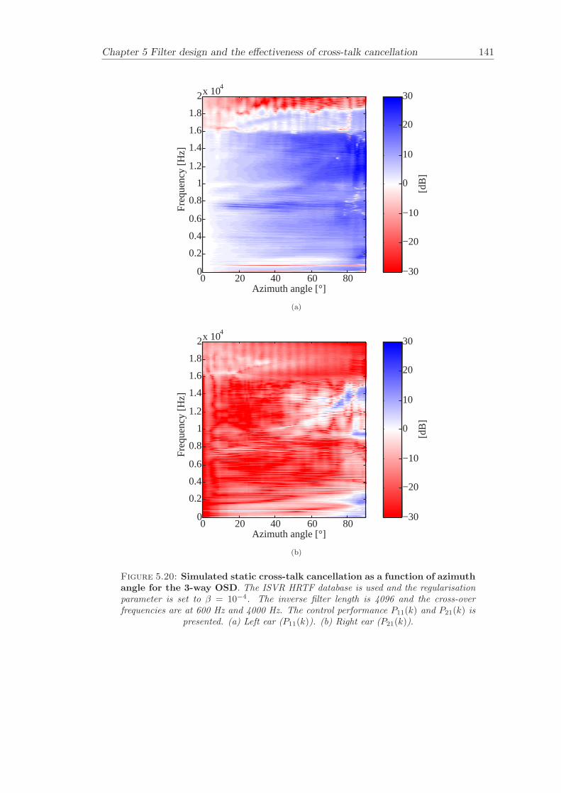
Chapter 5 Filter design and the effectiveness of cross-talk cancellation 141
Fre
quen
cy [H
z]
Azimuth angle [°]0 20 40 60 80
0
0.2
0.4
0.6
0.8
1
1.2
1.4
1.6
1.8
2x 10⁴
[dB
]
−30
−20
−10
0
10
20
30
(a)
Fre
quen
cy [H
z]
Azimuth angle [°]0 20 40 60 80
0
0.2
0.4
0.6
0.8
1
1.2
1.4
1.6
1.8
2x 10⁴
[dB
]
−30
−20
−10
0
10
20
30
(b)
Figure 5.20: Simulated static cross-talk cancellation as a function of azimuthangle for the 3-way OSD. The ISVR HRTF database is used and the regularisationparameter is set to β = 10−4. The inverse filter length is 4096 and the cross-overfrequencies are at 600 Hz and 4000 Hz. The control performance P11(k) and P21(k) is
presented. (a) Left ear (P11(k)). (b) Right ear (P21(k)).
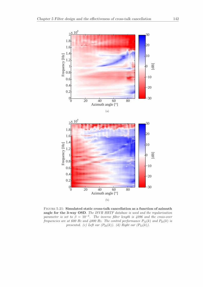
Chapter 5 Filter design and the effectiveness of cross-talk cancellation 142
Fre
quen
cy [H
z]
Azimuth angle [°]0 20 40 60 80
0
0.2
0.4
0.6
0.8
1
1.2
1.4
1.6
1.8
2x 10⁴
[dB
]
−30
−20
−10
0
10
20
30
(a)
Fre
quen
cy [H
z]
Azimuth angle [°]0 20 40 60 80
0
0.2
0.4
0.6
0.8
1
1.2
1.4
1.6
1.8
2x 10⁴
[dB
]
−30
−20
−10
0
10
20
30
(b)
Figure 5.21: Simulated static cross-talk cancellation as a function of azimuthangle for the 3-way OSD. The ISVR HRTF database is used and the regularisationparameter is set to β = 10−4. The inverse filter length is 4096 and the cross-overfrequencies are at 600 Hz and 4000 Hz. The control performance P12(k) and P22(k) is
presented. (c) Left ear (P22(k)). (d) Right ear (P12(k)).
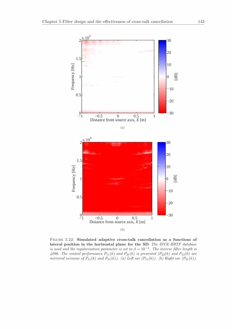
Chapter 5 Filter design and the effectiveness of cross-talk cancellation 143
Fre
quen
cy [H
z]
Distance from source axis, X [m]−1 −0.5 0 0.5 10
0.5
1
1.5
2x 10
4
[dB
]
−30
−20
−10
0
10
20
30
(a)
Fre
quen
cy [H
z]
Distance from source axis, X [m]−1 −0.5 0 0.5 10
0.5
1
1.5
2x 10
4
[dB
]
−30
−20
−10
0
10
20
30
(b)
Figure 5.22: Simulated adaptive cross-talk cancellation as a functions oflateral position in the horizontal plane for the SD. The ISVR HRTF databaseis used and the regularisation parameter is set to β = 10−4. The inverse filter length is4096. The control performance P11(k) and P21(k) is presented (P22(k) and P12(k) aremirrored versions of P11(k) and P21(k)). (a) Left ear (P11(k)). (b) Right ear (P21(k)).
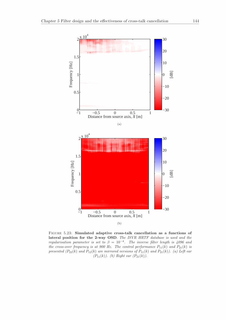
Chapter 5 Filter design and the effectiveness of cross-talk cancellation 144
Fre
quen
cy [H
z]
Distance from source axis, X [m]−1 −0.5 0 0.5 10
0.5
1
1.5
2x 10
4
[dB
]
−30
−20
−10
0
10
20
30
(a)
Fre
quen
cy [H
z]
Distance from source axis, X [m]−1 −0.5 0 0.5 10
0.5
1
1.5
2x 10
4
[dB
]
−30
−20
−10
0
10
20
30
(b)
Figure 5.23: Simulated adaptive cross-talk cancellation as a functions oflateral position for the 2-way OSD. The ISVR HRTF database is used and theregularisation parameter is set to β = 10−4. The inverse filter length is 4096 andthe cross-over frequency is at 900 Hz. The control performance P11(k) and P21(k) ispresented (P22(k) and P12(k) are mirrored versions of P11(k) and P21(k)). (a) Left ear
(P11(k)). (b) Right ear (P21(k)).
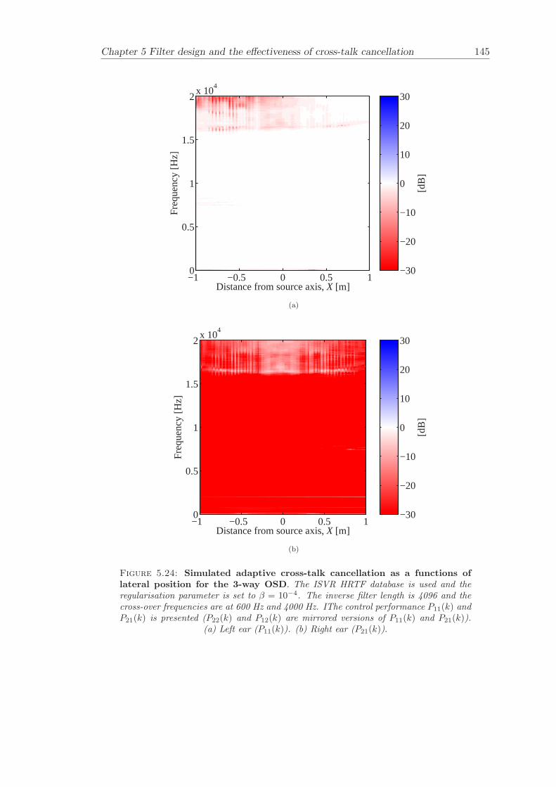
Chapter 5 Filter design and the effectiveness of cross-talk cancellation 145
Fre
quen
cy [H
z]
Distance from source axis, X [m]−1 −0.5 0 0.5 10
0.5
1
1.5
2x 10
4
[dB
]
−30
−20
−10
0
10
20
30
(a)
Fre
quen
cy [H
z]
Distance from source axis, X [m]−1 −0.5 0 0.5 10
0.5
1
1.5
2x 10
4
[dB
]
−30
−20
−10
0
10
20
30
(b)
Figure 5.24: Simulated adaptive cross-talk cancellation as a functions oflateral position for the 3-way OSD. The ISVR HRTF database is used and theregularisation parameter is set to β = 10−4. The inverse filter length is 4096 and thecross-over frequencies are at 600 Hz and 4000 Hz. IThe control performance P11(k) andP21(k) is presented (P22(k) and P12(k) are mirrored versions of P11(k) and P21(k)).
(a) Left ear (P11(k)). (b) Right ear (P21(k)).
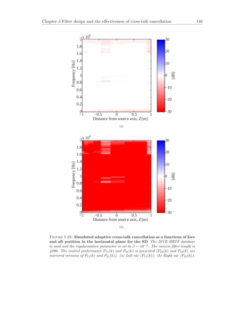
Chapter 5 Filter design and the effectiveness of cross-talk cancellation 146
Fre
quen
cy [H
z]
Distance from source axis, Z [m]−1 −0.5 0 0.5 10
0.2
0.4
0.6
0.8
1
1.2
1.4
1.6
1.8
2x 10⁴
[dB
]
−30
−20
−10
0
10
20
30
(a)
Fre
quen
cy [H
z]
Distance from source axis, Z [m]−1 −0.5 0 0.5 10
0.2
0.4
0.6
0.8
1
1.2
1.4
1.6
1.8
2x 10⁴
[dB
]
−30
−20
−10
0
10
20
30
(b)
Figure 5.25: Simulated adaptive cross-talk cancellation as a functions of foreand aft position in the horizontal plane for the SD. The ISVR HRTF databaseis used and the regularisation parameter is set to β = 10−4. The inverse filter length is4096. The control performance P11(k) and P21(k) is presented (P22(k) and P12(k) aremirrored versions of P11(k) and P21(k)). (a) Left ear (P11(k)). (b) Right ear (P21(k)).

Chapter 5 Filter design and the effectiveness of cross-talk cancellation 147
Fre
quen
cy [H
z]
Distance from source axis, Z [m]−1 −0.5 0 0.5 10
0.5
1
1.5
2x 10
4
[dB
]
−30
−20
−10
0
10
20
30
(a)
Fre
quen
cy [H
z]
Distance from source axis, Z [m]−1 −0.5 0 0.5 10
0.5
1
1.5
2x 10
4
[dB
]
−30
−20
−10
0
10
20
30
(b)
Figure 5.26: Simulated adaptive cross-talk cancellation as a functions offore and aft position for the 2-way OSD. The ISVR HRTF database is used andthe regularisation parameter is set to β = 10−4. The inverse filter length is 4096 andthe cross-over frequency is at 900 Hz. The control performance P11(k) and P21(k) ispresented (P22(k) and P12(k) are mirrored versions of P11(k) and P21(k)). (a) Left ear
(P11(k)). (b) Right ear (P21(k)).
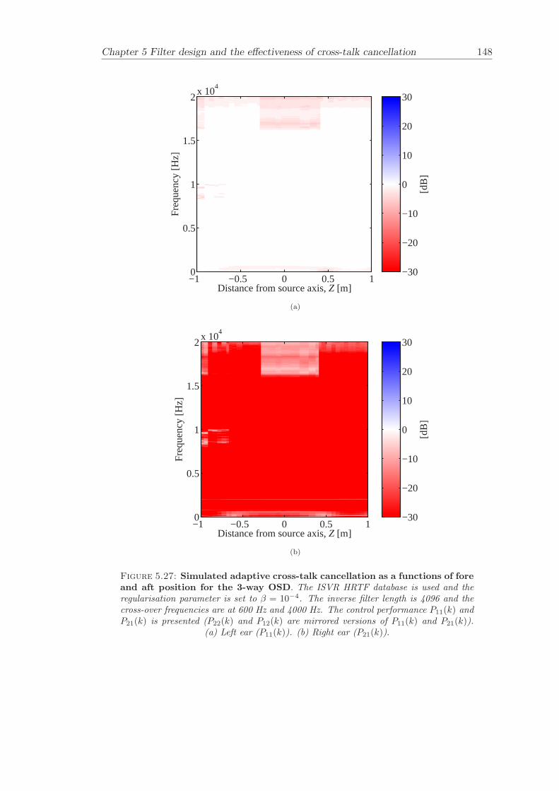
Chapter 5 Filter design and the effectiveness of cross-talk cancellation 148
Fre
quen
cy [H
z]
Distance from source axis, Z [m]−1 −0.5 0 0.5 10
0.5
1
1.5
2x 10
4
[dB
]
−30
−20
−10
0
10
20
30
(a)
Fre
quen
cy [H
z]
Distance from source axis, Z [m]−1 −0.5 0 0.5 10
0.5
1
1.5
2x 10
4
[dB
]
−30
−20
−10
0
10
20
30
(b)
Figure 5.27: Simulated adaptive cross-talk cancellation as a functions of foreand aft position for the 3-way OSD. The ISVR HRTF database is used and theregularisation parameter is set to β = 10−4. The inverse filter length is 4096 and thecross-over frequencies are at 600 Hz and 4000 Hz. The control performance P11(k) andP21(k) is presented (P22(k) and P12(k) are mirrored versions of P11(k) and P21(k)).
(a) Left ear (P11(k)). (b) Right ear (P21(k)).
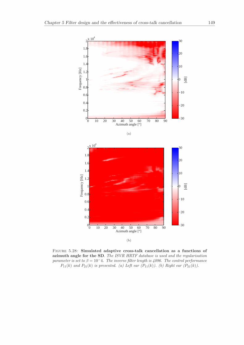
Chapter 5 Filter design and the effectiveness of cross-talk cancellation 149
Fre
quen
cy [H
z]
Azimuth angle [°]0 10 20 30 40 50 60 70 80 90
0
0.2
0.4
0.6
0.8
1
1.2
1.4
1.6
1.8
2x 10
4
[dB
]
−30
−20
−10
0
10
20
30
(a)
Fre
quen
cy [H
z]
Azimuth angle [°]0 10 20 30 40 50 60 70 80 90
0
0.2
0.4
0.6
0.8
1
1.2
1.4
1.6
1.8
2x 10
4
[dB
]
−30
−20
−10
0
10
20
30
(b)
Figure 5.28: Simulated adaptive cross-talk cancellation as a functions ofazimuth angle for the SD. The ISVR HRTF database is used and the regularisationparameter is set to β = 10−4. The inverse filter length is 4096. The control performance
P11(k) and P21(k) is presented. (a) Left ear (P11(k)). (b) Right ear (P21(k)).
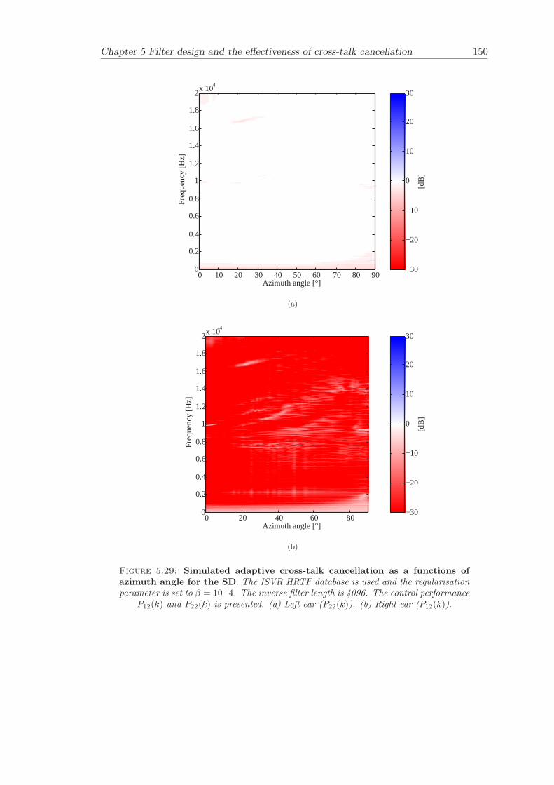
Chapter 5 Filter design and the effectiveness of cross-talk cancellation 150
Fre
quen
cy [H
z]
Azimuth angle [°]0 10 20 30 40 50 60 70 80 90
0
0.2
0.4
0.6
0.8
1
1.2
1.4
1.6
1.8
2x 10
4
[dB
]
−30
−20
−10
0
10
20
30
(a)
Fre
quen
cy [H
z]
Azimuth angle [°]0 20 40 60 80
0
0.2
0.4
0.6
0.8
1
1.2
1.4
1.6
1.8
2x 10
4
[dB
]
−30
−20
−10
0
10
20
30
(b)
Figure 5.29: Simulated adaptive cross-talk cancellation as a functions ofazimuth angle for the SD. The ISVR HRTF database is used and the regularisationparameter is set to β = 10−4. The inverse filter length is 4096. The control performance
P12(k) and P22(k) is presented. (a) Left ear (P22(k)). (b) Right ear (P12(k)).

Chapter 5 Filter design and the effectiveness of cross-talk cancellation 151
Fre
quen
cy [H
z]
Azimuth angle [°]0 10 20 30 40 50 60 70 80 90
0
0.2
0.4
0.6
0.8
1
1.2
1.4
1.6
1.8
2x 10
4
[dB
]
−30
−20
−10
0
10
20
30
(a)
Fre
quen
cy [H
z]
Azimuth angle [°]0 10 20 30 40 50 60 70 80 90
0
0.2
0.4
0.6
0.8
1
1.2
1.4
1.6
1.8
2x 10
4
[dB
]
−30
−20
−10
0
10
20
30
(b)
Figure 5.30: Simulated adaptive cross-talk cancellation as a functions ofazimuth angle for the 2-way OSD. The ISVR HRTF database is used and theregularisation parameter is set to β = 10−4. The inverse filter length is 4096 andthe cross-over frequency is at 900 Hz. The control performance P11(k) and P21(k) is
presented. (a) Left ear (P11(k)). (b) Right ear (P21(k)).
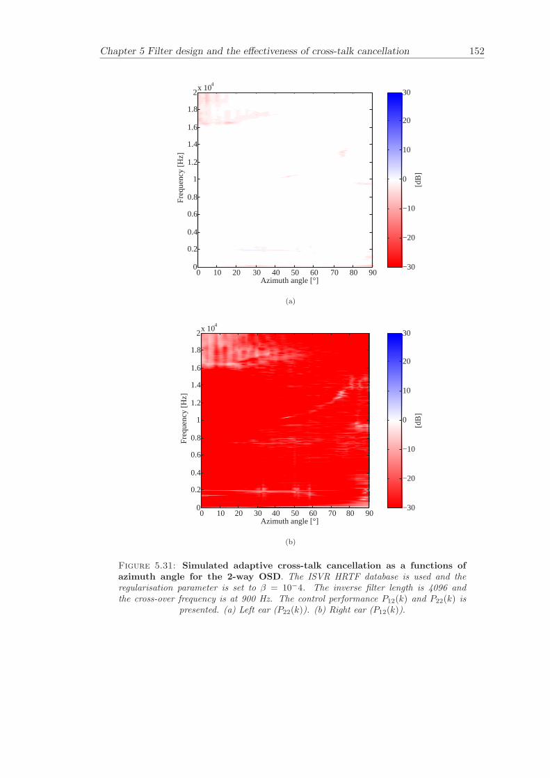
Chapter 5 Filter design and the effectiveness of cross-talk cancellation 152
Fre
quen
cy [H
z]
Azimuth angle [°]0 10 20 30 40 50 60 70 80 90
0
0.2
0.4
0.6
0.8
1
1.2
1.4
1.6
1.8
2x 10
4
[dB
]
−30
−20
−10
0
10
20
30
(a)
Fre
quen
cy [H
z]
Azimuth angle [°]0 10 20 30 40 50 60 70 80 90
0
0.2
0.4
0.6
0.8
1
1.2
1.4
1.6
1.8
2x 10
4
[dB
]
−30
−20
−10
0
10
20
30
(b)
Figure 5.31: Simulated adaptive cross-talk cancellation as a functions ofazimuth angle for the 2-way OSD. The ISVR HRTF database is used and theregularisation parameter is set to β = 10−4. The inverse filter length is 4096 andthe cross-over frequency is at 900 Hz. The control performance P12(k) and P22(k) is
presented. (a) Left ear (P22(k)). (b) Right ear (P12(k)).

Chapter 5 Filter design and the effectiveness of cross-talk cancellation 153
Fre
quen
cy [H
z]
Azimuth angle [°]0 10 20 30 40 50 60 70 80 90
0
0.2
0.4
0.6
0.8
1
1.2
1.4
1.6
1.8
2x 10
4
[dB
]
−30
−20
−10
0
10
20
30
(a)
Fre
quen
cy [H
z]
Azimuth angle [°]0 10 20 30 40 50 60 70 80 90
0
0.2
0.4
0.6
0.8
1
1.2
1.4
1.6
1.8
2x 10
4
[dB
]
−30
−20
−10
0
10
20
30
(b)
Figure 5.32: Simulated adaptive cross-talk cancellation as a functions ofazimuth angle for the 3-way OSD. The ISVR HRTF database is used and theregularisation parameter is set to β = 10−4. The inverse filter length is 4096 and thecross-over frequencies are at 600 Hz and 4000 Hz. The control performance P11(k) and
P21(k) is presented. (a) Left ear (P11(k)). (b) Right ear (P21(k)).

Chapter 5 Filter design and the effectiveness of cross-talk cancellation 154
Fre
quen
cy [H
z]
Azimuth angle [°]0 10 20 30 40 50 60 70 80 90
0
0.2
0.4
0.6
0.8
1
1.2
1.4
1.6
1.8
2x 10
4
[dB
]
−30
−20
−10
0
10
20
30
(a)
Fre
quen
cy [H
z]
Azimuth angle [°]0 10 20 30 40 50 60 70 80 90
0
0.2
0.4
0.6
0.8
1
1.2
1.4
1.6
1.8
2x 10
4
[dB
]
−30
−20
−10
0
10
20
30
(b)
Figure 5.33: Simulated adaptive cross-talk cancellation as a functions ofazimuth angle for the 3-way OSD. The ISVR HRTF database is used and theregularisation parameter is set to β = 10−4. The inverse filter length is 4096 and thecross-over frequencies are at 600 Hz and 4000 Hz. The control performance P11(k) and
P21(k) is presented. (a) Left ear (P11(k)). (b) Right ear (P21(k)).
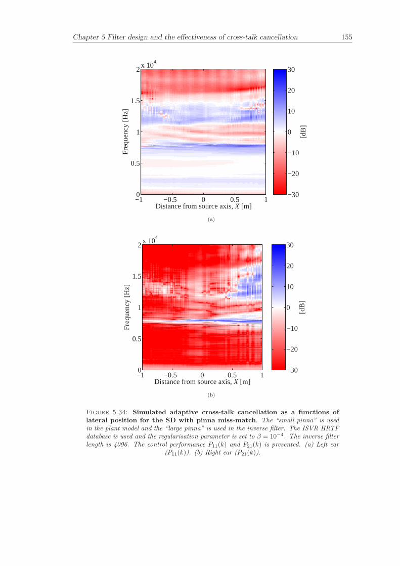
Chapter 5 Filter design and the effectiveness of cross-talk cancellation 155
Fre
quen
cy [H
z]
Distance from source axis, X [m]−1 −0.5 0 0.5 10
0.5
1
1.5
2x 10
4
[dB
]
−30
−20
−10
0
10
20
30
(a)
Fre
quen
cy [H
z]
Distance from source axis, X [m]−1 −0.5 0 0.5 10
0.5
1
1.5
2x 10
4
[dB
]
−30
−20
−10
0
10
20
30
(b)
Figure 5.34: Simulated adaptive cross-talk cancellation as a functions oflateral position for the SD with pinna miss-match. The “small pinna” is usedin the plant model and the “large pinna” is used in the inverse filter. The ISVR HRTFdatabase is used and the regularisation parameter is set to β = 10−4. The inverse filterlength is 4096. The control performance P11(k) and P21(k) is presented. (a) Left ear
(P11(k)). (b) Right ear (P21(k)).
Chapter 6
Filter update techniques and
subjective experiments
Filter updates are necessary when the listener is moving out of the “sweet-spot” sincethe transfer functions between the listener and the loudspeakers change with position.Two filter update techniques are presented and evaluated, namely direct filter updatesusing pre-computed inverse filters and filter updates using a reduced database of transferfunctions. The filter update rate is an important parameter for virtual sound imagingsystems, and determines how often the filter coefficients need to be updated so that theupdates can be seamless for the listener. The filter update rate is determined here bydefining two criteria: the Just Noticeable Difference (JND) criterion and the Just No-ticeable Change (JNC) criterion. The JNC criterion determines the maximum distancebetween filter updates that does not create any audible signal changes for the listener.For example if the listener is changing position and the filter is updated on a too coarsegrid then a noticeable “click” sound will appear. Hence, the JNC criterion determinesthe step size of the filter updates in the commutation process and aims to remove audibleartifacts. The JND criterion determines the maximum distance between filter updatesthat does not create any changes in the virtual sound image perceived by the listener.For example if the listener is changing position and the filter is updated on a too coarsegrid then it is perceived as if the virtual sound source is changing position while it is notintended to do so. The JND and JNC criteria for filter updates are determined througha set of subjective experiments.
The interpolation process is typically associated with the synthesis of an intermediatetransfer function from a database of predefined filters. If a reduced database of transferfunctions is used, the interpolation process serves to fill in the associated gaps. Com-mutation is the process of updating the filter coefficients in real-time while the filter isrunning (Jot [44]). The filter update can cause audible artifacts and the commutationprocess can remove those.
156
Chapter 6 Filter update techniques and subjective experiments 157
Filter updates can be dealt with by using different techniques. A common technique is“cross-fading” that uses two filters in parallel, and the output is computed as a weightedsum of the outputs from the filters using linear interpolation (Huopaniemi [38]). Thefilter update transition time is the time it takes to completely change the output fromthe current filter to the new filter. This technique doubles the computational cost of thefilter implementation. The filters can be implemented by using techniques such as FIR,WFIR, IIR and WIIR among others (Karjalainen [45], Farina [29], Jot [44]). Anotherfilter update technique that limits transients has been presented by Valimaki [99] andis based on state variables for updating the IIR filter coefficients. This technique canreduce the computational cost of commutation by 50% compared to cross-fading twofilters in parallel.
Rose [86] conducted subjective experiments in order to determine a filter update criterionfor an adaptive SD system. The results show that the filter update criterion is about 0.03m to achieve the most stable virtual sound images. It was also found that virtual soundimage locations far from the loudspeakers require a smaller “filter update movementincrement” criterion than virtual sound images close to the loudspeakers. The “filterupdate movement increment” is similar to the JND criterion determined here.
Localisation blur is defined as the threshold for detecting changes in virtual sourceangles. A survey for localisation blur in the horizontal plane is presented by Blauert [13]where the localisation blur varies between 1.4 and 3.3 for broadband/narrowbandnoise signals. The localisation blur studies could be used to form a JND criterionusing an objective evaluation of the filter updates. Moore [70] points out that thesmallest detectable intensity change for wide-band noise and band-pass filtered noiseis approximately a constant fraction of the intensity of the stimulus. This fractionis called Weber’s law, which states that the smallest detectable change in a stimulusis proportional to the magnitude of the stimulus. The smallest detectable change forbroadband noise is about 0.5 - 1 dB. This could be used as an alternative method toform a JNC criterion for the filter updates.
6.1 A review of alternative filter update techniques
The problem of updating inverse filters in real-time can be resolved by using the followingtwo alternative techniques, direct filter updates using pre-computed inverse filters andfilter updates using a reduced database of transfer functions. The presented filter updatetechniques uses direct filter coefficient updates for a total of four FIR filters to implementadaptive cross-talk cancellation for a single listener. These techniques require only halfthe computational cost for the filter updates compared to cross-fading that uses twofilters in parallel. The filter update techniques can be used with both SD and FDL typeof systems by using superposition of the different frequency bands as described in Section
Chapter 6 Filter update techniques and subjective experiments 158
5.1 in the FDL case. A block diagram of the adaptive virtual sound imaging system ispresented in Figure 6.1. The signals and transfer functions in Figure 6.1 are defined asfollows. The transducers produce source strengths from the input voltages defined by theelements of the complex vector v(k) = [V1(k) V2(k)]T . The resulting acoustic pressuresignals are defined by the vector w(k) = [W1(k) W2(k)]T . The transfer functions fora generelised binaural sound reproduction system as a function of time t are namedΨt(k) and the corresponding inverse transfer functions are named Πt(k). The acousticpressure signals are found by
w(k) = Ψt(k)v(k) (6.1)
The two signals to be reproduced at the listener’s ears are defined by the complex vectord(k) = [D1(k) D2(k)]T . The desired signals d(k) to be reproduced is a delayed versionof the recorded or synthesised signals u(k), hence d(k) = u(k)e−jω∆. The signals u(k)can be obtained from a dummy head recording or from filtering signals x(k) by a matrixof binaural filters A(k) = [A1(k) A2(k)]T . The source strengths can now be found by
v(k) = Πt(k)d(k) (6.2)
where Πt(k) contains inverse filters that also change with time t as the listener enters anew position such that
Πt(k) =
[Π11t(k)Π21t(k)
Π12t(k)Π22t(k)
](6.3)
and thus
w(k) = Πt(k)Ψt(k)d(k) (6.4)
where
Ψt(k) =
[Ψ11t(k)Ψ21t(k)
Ψ12t(k)Ψ22t(k)
](6.5)
6.1.1 Direct filter updates
The results from the subjective filter update experiment for JNC in Section 6.2 can beused to establish a technique based on direct updates of inverse filters. The direct updateof inverse filter technique works by using a large database of pre-computed inverse filters
Chapter 6 Filter update techniques and subjective experiments 159
(look-up table) that are updated at steps of the JNC criterion for lateral movement.Hence, as the listener moves the inverse filters that correspond to the geometry of theloudspeakers and the listener are updated at the JNC criteria for lateral movement. Thetechnique is based on filter coefficient updates. The algorithm essentially picks up theinverse filters that correspond to the position the listener that is located with a precisioncorresponding to the JNC criterion and then updates the filter coefficients accordingly.The advantage of this technique is that it requires only a small amount of computingpower for updating the filters. The disadvantage is that it requires a large database ofinverse filters, which increases the memory requirements.
6.1.1.1 Summary of algorithm
The database contains inverse filters for pre-defined listener positions that are spacedaccording to the JNC criterion.
(1) Acquire the listener position from the head tracker.
(2) If the threshold for filter update is breached, then update the inverse filters Πt(k)directly at an update rate, which ideally is equal to or greater than the filter decay time(the number of FIR filter coefficients multiplied by the sampling period). The thresholdis based on the JNC criterion.
(3) Return to (1).
Note that if the precision of the tracking system can not match the JNC criterion then itis possible establish an appropriate filter update threshold. The filter update thresholdshould ideally never exceed the JND criterion. The filter update is then carried outby performing commutation in between the new and the old listener position usingpre-computed filters.
6.1.2 Filter updates using a reduced database of transfer functions
A filter update algorithm is presented that can reduce the size of the database to aminimum in terms of filter design positions. The technique uses commutation and real-time inversion. The reduced database holds only transfer functions for three listenerpositions in the lateral plane. The three sets of HRIRs correspond to the far end ofeach direction of the lateral plane where the listener is allowed to move and the centreposition. The transfer functions in the database are denoted Ψl(k),Ψc(k),Ψr(k) wherel represents the far left position, c represents the centre position and r corresponds tothe far right position. The listener can in this example move ±0.7 m in the lateral planerelative to on-axis at a distance of 2 m in the fore and aft plane. The amount of listenermovement is established by allowing interpolation for azimuth angles up to 20. This
Chapter 6 Filter update techniques and subjective experiments 160
will ensure that the average mean square interpolation error is less than about 1.74%,which is valid for frontal directions as stated in Table 4.1.
The HRIRs are stored in an ITD-equalised state such that interpolation can be applieddirectly to the coefficients. The interpolation is performed by using linear interpolationas described in Section 4.1. The appropriate amount of delay is inserted after theinterpolation stage using a delay line. The delay line should be able to handle fractionaldelays (Laakso [57]) if the sampling rate is lower than approximately 100 kHz, since theITD threshold is approximately 10 µs (Klumpp and Eady [52]). The algorithm computesthe inverse filters in between two pre-measured filters in the database to achieve aspacing of no less than the JNC criterion during the filter update. The inverse filters arecomputed using the fast-deconvolution algorithm. A filter update is initiated every timethe JND criterion is breached by the tracker. When a filter update is initiated, then theinverse filters are computed with a spacing of the JNC criterion in between the old andthe new filter positions that has a spacing of the JND criterion. The number of inversefilters during update is given by Nu = 1/((JNC mod JND)/JND). When the new inversefilters are available then the filters are updated with a step size of the JNC criterionand at an update rate that ideally is equal to or greater than the filter decay time.The advantage of this method is the reduced size of the database of transfer functions.The disadvantage with commutation between filters using a reduced database is thecomputational overhead that the interpolation and the fast-deconvolution algorithm areimposing.
6.1.2.1 Summary of algorithm
The spacing of the database is 20 in azimuth angle as in the simulation in Figure 4.4.
(1) Get the new listener position from the head tracker.
(2) If the threshold for filter update is breached, then compute Nu new sets of inversefilters Π1(k),...,ΠNu(k) using the fast-deconvolution algorithm and the database withtransfer functions Ψl(k),Ψc(k),Ψr(k). The new set of inverse filter positions are spacedwith the JNC criterion. The two transfer functions that are the nearest neighbours tothe new position are used for computing the new set of inverse filters.
(3) Update the inverse filters Πt(k) at an update rate, which ideally is equal to or greaterthan the filter decay time.
(4) Return to (1).
Chapter 6 Filter update techniques and subjective experiments 161
6.2 Subjective evaluation of filter update techniques
The filter update criteria are determined through a series of subjective experiments car-ried out both under anechoic conditions and in a listening room. The intended filterdesign position was moved relative to the listener at carefully controlled rates. The in-tended filter design position is defined as the position where the listener is ideally locatedfor the cross-talk cancellation process to perform optimally. When the intended filterdesign position is moved away from the centre of the listener, then the performance ofthe cross-talk cancellation process starts to degrade, which in turn leads to a degradationin the sound source localisation ability of the listener. The listeners were wearing a maskin front of their eyes so that no visual cues were available. The subjective experimentsthat have been carried out here applies directly to the filter update techniques presentedin Section 6.1.
A filter update criterion for an adaptive SD system was determined in a set of ex-periments by Rose [87]. The virtual imaging system was moved in the lateral planein front of several subjects. The first experiment was performed for determining the“sweet-spot” size in a static case, where the subjects had a fixed position and the SDwas moved into different positions in the lateral plane. The sound source localizationability was determined by asking the subject for the perceived angle of a virtual source.The results from this experiment show that the maximum tolerable distance betweenfilter updates is about 0.03 m. The objective of the second experiment was to find thethreshold parameters necessary for two real moving sound sources to produce a station-ary virtual sound image. The subjects in the experiment were asked to respond to boththe location and the stability of the virtual sound image as the SD was moving and thefilters were updated. The results show that filter update increments corresponding tolateral movements less than 0.03 m achieve the most stable virtual sound image of theexamined increments. Above this filter update rate, there was a steady deterioration ofthe stability of the virtual sound image.
A set of subjective experiments has been carried out to determine JND and JNC forbinaural sound reproduction using loudspeakers under both anechoic and more realis-tic conditions (listening room). Firstly, the electro-acoustic transfer functions of theloudspeaker were measured at asymmetric listener positions. The loudspeaker systemthat was used is a 4-way FDL with the following source spans 2θ: 5.8, 15.4, 41.2
and 57.6. The transfer functions were measured with a spacing of 0.025 m both in thelateral plane (−0.175 ≤ X ≤ 0.175) and in the fore and aft plane (−0.175 ≤ Z ≤ 0.175)using the KEMAR dummy head. The transfer functions were interpolated to achieve aspacing of 0.0125 m by using the interpolation algorithm described in Section 4.1. Theninverse filters for the listener positions were designed. Finally, the cross-talk cancella-tion performance was verified and filter update rates were determined by the subjectiveexperiments presented in Section 6.2.1 and Section 6.2.2.
Chapter 6 Filter update techniques and subjective experiments 162
6.2.1 Filter update rates under anechoic conditions
A subjective experiment was carried out in order to determine the JND and JNC criteria.The binaural stimuli was created by convolving band limited white noise (300 Hz - 3000Hz) with a set HRTFs corresponding to a virtual source at 40 to the right of the listener.The upper limit of the band-pass filter was chosen to 3000 Hz and the lower limit ofthe band-pass filter was chosen to cut off frequencies below 300 Hz. The “pinna notch”was excluded in order minimize uncertainties regarding differences between the subject’spinnae. It is noted that the high-pass cross-over frequency for the high frequency unit ofthe 4-way FDL is 4000 Hz, hence the high frequency unit did not contribute to the resultsin this experiment. The binaural stimuli for the JND criterion were convolved with thecross-talk cancellation filters for the intended filter design positions and recorded to aCD that was played back to the subjects. The stimuli for the JNC criterion was createdby updating the FIR filters with the Huron work station and recording using a DigitalAudio Tape (DAT) player and a KEMAR dummy head (Burkard [16]). The recordedbinaural stimuli was then convolved with cross-talk cancellation filters and recorded toa CD, which was played back to the subjects. The JNC criterion that determines themaximum distance between filter updates was evaluated for an update rate of 0.05 m/sfor changing the intended filter design position. The experiments were carried out bychanging only the intended filter design position while the listener and the loudspeakersstayed in fixed positions.
The JND criterion was investigated by presenting a virtual noise source to the listenerand changing the intended filter design position. The intended filter design positionwas changed in the lateral plane from −0.175 ≤ X ≤ 0.175 m with a spacing of 0.0125m. Hence, the position was changed more than half a head width. The experimentwas carried out by changing the intended filter design position in four directions asillustrated in Figure 6.2. The stimuli were convolved with the filter for each intendeddesign position such that a virtual source at φ = 40 to the right would appear forthe subject. The stimuli were presented for one second at each intended filter designposition and after the stimuli a pause of five seconds was imposed so that the subjectcould point the perceived angle of the virtual noise source.
The JNC criterion was investigated by presenting a virtual noise source and changingthe intended filter design position dynamically. The stimuli were convolved with thefilter for each intended design position such that a virtual noise source at φ = 40 tothe right appeared for the subject. The intended filter design position was switched inthe lateral plane between two positions, where one of the positions was the centre of thehead and the other an off-axis position. The spacing between the two positions was asfollows: 0.0125 m, 0.025 m, 0.0375 m, 0.05 m and 0.065 m. The stimuli were presentedfor five seconds while the intended filter design positions were switched back and forth.After the stimuli a pause of five seconds was imposed such that the subject could report
Chapter 6 Filter update techniques and subjective experiments 163
if the filter changes were audible or not. The intended filter design position was changedin the lateral directions (3) and (4) as illustrated in Figure 6.2.
A preliminary subjective experiment was carried out in the fore and aft plane, in order todetermine the JND criterion in this direction. The experiment was carried out using thesame process as in the lateral plane. The JND criterion was investigated by presentinga virtual noise source at φ = 40 to the right of the listener as in the previous case.The experiment was carried out by changing the intended filter design position in fourdirections as illustrated in Figure 6.3.
The results presented are from fifteen subjects out of twenty, where data from five ofthe subjects was disregarded by performing an ANOVA (Analysis of Variance) test.The Matlab [65] function anova1() was used for carrying out the ANOVA test witha p-value (“statistical significance” measure) of 0.05. The subjective responses in thelateral plane of the virtual source localisation test in the JND experiment is presentedin Figure 6.4. The mean values and standard deviation from fourteen measurementpoints in the lateral plane with a spacing of 0.0125 m is presented for four directionsof movement. Now the individual off-axis positions were investigated starting withX = 0.025 in order to determine the JND criterion with a certain amount of probability.Figure 6.5 illustrates the data for an off-axis listener position of 0.025 m. The meanvirtual source localisation change for this off-axis position is 2.3 and the standarddeviation is 4.0. The combined data from all of the four types of movements were usedhere. The data was un-biased such that the directionality of the virtual source anglechange was the same for all investigated directions of movement. Here, the localisationblur is defined as the amount of displacement of the position of the virtual sound sourcethat is recognised by 50% of the subjects as a change in the the position of the auditoryevent. This definition is common practice in psychoacoustics (Blauert [13]). Under theassumption of a normal distribution, for 50% probability of a stable virtual sound image,then the localisation blur must be no less than ±3.2. Then the off-axis position of X =0.0375 was investigated and it was found that the mean virtual source localisation changeis 5.6 and the standard deviation is 5.8, which is greater than in the localisation blurstudies summarised by Blauert [13]. Hence, the result from the JND experiment in thelateral plane suggests that the inverse filters should be updated as often as approximately0.025 m for the sound image to be stable with respect to virtual source angle.
The subjective responses for the JNC experiment is illustrated in Figure 6.6. Thehistogram shows the probability density of the data that was collected in the anechoicchamber. The assumption was made that the threshold for detecting filter change is inbetween the two readings where the subjects could detect the filter change and wherethey could not detect it. For example, a subject that could detect filter change witha filter update rate of 0.025 m but not detect a filter update rate of 0.0125 m, thenthe threshold is given by (0.025-0.0125/2)=0.01875 m. Here, the mean value of thedata is 0.016 m. The probability density of the collected data was then represented by
Chapter 6 Filter update techniques and subjective experiments 164
the lognormal probability density function as illustrated in Figure 6.6 (b). The meanand standard deviation associated with the lognormal function was estimated usingthe Maximum Likelihood Estimator (MLE) function mle in Matlab [65]. Under theassumption that the collected data can be represented by a lognormal distribution, for50% probability of not detecting any filter change, then the JNC threshold is 0.012 min the anechoic case. The result from the JNC experiment in the lateral plane suggeststhat the inverse filters using the direct filter update technique should be updated moreoften than 0.012 m.
The result from the JND experiment in the fore and aft plane suggests that the inversefilters can be updated less often than 0.15 m for the image to be stable with respect tovirtual source angle. This can be expected, since the ITD does not change significantlyin the fore and aft direction. The subjective response for JND in the fore and aft planeis presented in Figure 6.7.
6.2.2 Filter update rates in a listening room
This section determines filter update rates through a series of subjective experimentscarried out under realistic listening conditions with intended filter design positions movedrelative to the listener at carefully controlled rates. The experiment was carried outin the listening room at the ISVR, which was designed to be equivalent to realisticconditions for homes according to the IEC 268-13 standard. The procedures of theexperiment were the same as those described in Section 6.2 and was performed onfourteen subjects.
The results from the JND experiment in the listening room presented here are fromthirteen subjects out of fourteen. One of the subject’s data were disregarded by per-forming an ANOVA test as in Section 6.2.1. The results show good agreement betweenthe listening room and the anechoic chamber. The subjective response represented bymean values and standard deviation of virtual source localisation in the lateral plane ispresented in Figure 6.8. Again, the mean values and standard deviation from fourteenmeasurement points in the lateral plane with a spacing of 0.0125 m is presented for fourdirections of movement. Figure 6.9 illustrates the data for an off-axis listener positionof 0.025 m where the mean virtual source localisation change for position is 3.3 andlikewise the standard deviation is 3.3. Under the assumption of a normal distribution,for 50% probability of a stable virtual image, a localisation blur of ±3.4 must be al-lowed, which is close to the result for the anechoic case. The result from the subjectiveexperiment in the listening room shows that the inverse filters should be updated asoften as approximately 0.025 m for the image to be stable with respect to virtual sourceangle, as in the anechoic case.
Figure 6.10 illustrates the JNC data from the experiment that was carried out in the
Chapter 6 Filter update techniques and subjective experiments 165
listening room. The mean value of this data is 0.017 m. The data was processed pre-sented in the same way as for the anechoic case where the mean and standard deviationassociated with the lognormal function was estimated using the MLE. Under the as-sumption that the collected data can be represented by a lognormal distribution, for50% probability of not detecting any filter change, then the JNC threshold is 0.012 m inthe listening room. As in the anechoic case, the result from the JNC experiment showsthat the inverse filters using the direct filter update technique should be updated moreoften than 0.012 m.
The subjective experiment in the listening room shows no significant deviations fromthe anechoic chamber. The main difference that can be seen is the higher variancewhen the intended filter design position was far away from the on-axis position. This islikely to be a result of room reflections that makes the sound more diffuse. The resultsindicates that sound spatialisation using loudspeakers works well both under anechoicand non-anechoic listening conditions. The threshold for detecting filter changes wasalso very close to the anechoic case. This is likely to be due to the “precedence effect”that has a strong influence on sound source localisation ability. The precedence effectdescribes a group of phenomena that are used in resolving competition for perceptionand localisation between a reflection and direct sound (Litovskya [61]). In a reverberantenvironment such as the listening room the sound reach the ears by taking severaldifferent paths and although these reflections would be audible in isolation, the firstarriving wave front dominates the performance of sound source localisation.
6.3 Conclusion
Two different approaches to the solution of the problem of updating inverse filters in real-time have been proposed. The first and simplest technique is to update the inverse filtersdirectly by using an inverse filter database with a fine spacing that complies with theJNC criterion. This technique should be used when it is required that the computationalcost is low and when the memory can be relatively large. The second technique reducesthe database to a minimum by using real-time interpolation and real-time inversion forupdating the inverse filters. This technique should be used when it is required to havea small memory but the computational cost can be allowed to be relatively high. Thereduced database uses only filters for three listener positions in the lateral plane.
Filter update rates have been determined by defining the JND criterion and the JNCcriterion. The subjective evaluations in the anechoic chamber show that the JND cri-terion is approximately 0.025 m for movements in the lateral plane. The JNC criterionis approximately 0.012 m for movements in the lateral plane. The JND criterion formovements in the fore and aft plane is greater than the distance of ±0.15 m that wasexplored. A complementary subjective experiment was carried out in the listening room

Chapter 6 Filter update techniques and subjective experiments 166
using the same procedure as in the anechoic chamber. The results from the listeningroom showed no significant differences compared to the anechoic chamber. These resultssuggest that the filter update techniques and sound source localisation with loudspeakersworks well both under anechoic and non-anechoic listening conditions.
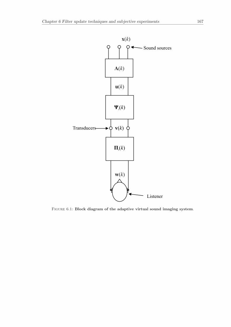
Chapter 6 Filter update techniques and subjective experiments 167
A( )k
w( )k
u( )k
x( )k
Transducers
Sound sources
Listener
v( )k
Ψt( )k
Πt( )k
Figure 6.1: Block diagram of the adaptive virtual sound imaging system.
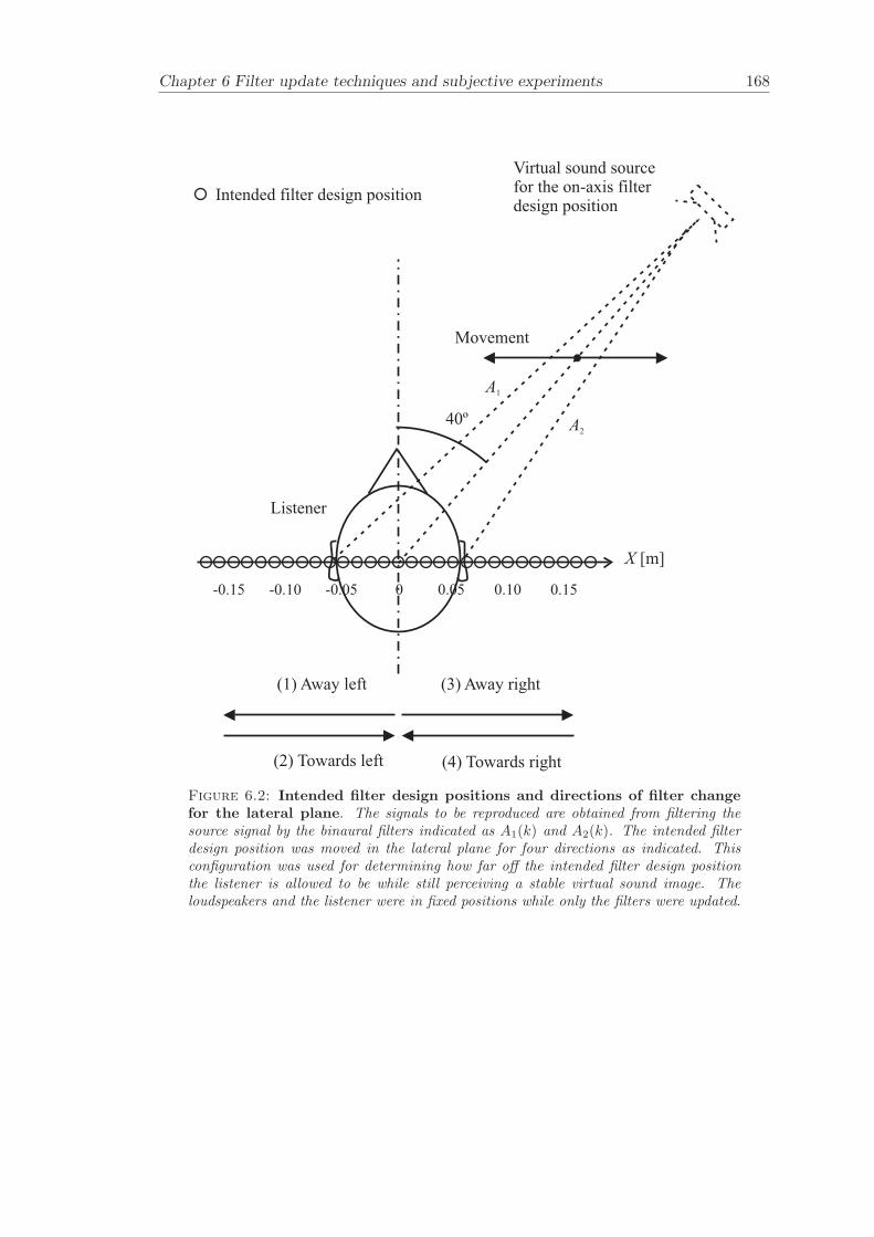
Chapter 6 Filter update techniques and subjective experiments 168
0 0.05 0.10 0.15-0.15 -0.10 -0.05
(2) Towards left
(1) Away left (3) Away right
(4) Towards right
Intended filter design position
X [m]
Virtual sound sourcefor the on-axis filterdesign position
40º
A1
A2
Listener
Movement
Figure 6.2: Intended filter design positions and directions of filter changefor the lateral plane. The signals to be reproduced are obtained from filtering thesource signal by the binaural filters indicated as A1(k) and A2(k). The intended filterdesign position was moved in the lateral plane for four directions as indicated. Thisconfiguration was used for determining how far off the intended filter design positionthe listener is allowed to be while still perceiving a stable virtual sound image. Theloudspeakers and the listener were in fixed positions while only the filters were updated.
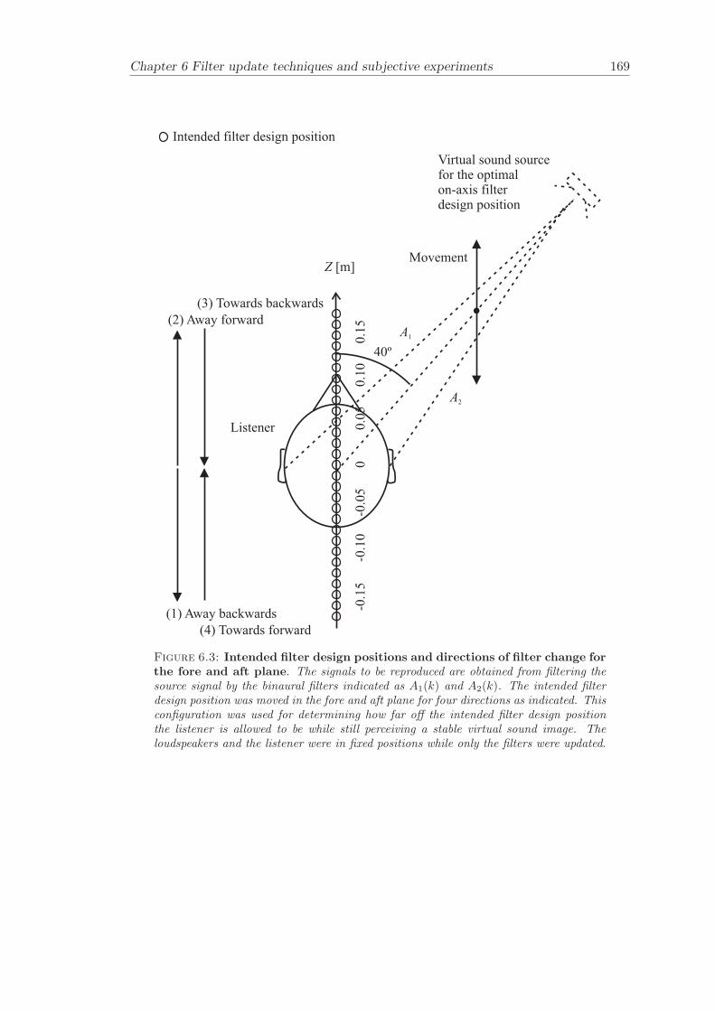
Chapter 6 Filter update techniques and subjective experiments 169
00
.05
0.1
00
.15
-0.1
5-0
.10
-0.0
5
Z [m]
(1) Away backwards
(2) Away forward
(3) Towards backwards
(4) Towards forward
Intended filter design position
Virtual sound sourcefor the optimalon-axis filterdesign position
40º
A1
A2
Listener
Movement
Figure 6.3: Intended filter design positions and directions of filter change forthe fore and aft plane. The signals to be reproduced are obtained from filtering thesource signal by the binaural filters indicated as A1(k) and A2(k). The intended filterdesign position was moved in the fore and aft plane for four directions as indicated. Thisconfiguration was used for determining how far off the intended filter design positionthe listener is allowed to be while still perceiving a stable virtual sound image. Theloudspeakers and the listener were in fixed positions while only the filters were updated.
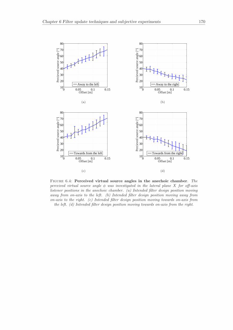
Chapter 6 Filter update techniques and subjective experiments 170
0 0.05 0.1 0.1510
20
30
40
50
60
70
80
Offset [m]
Per
ciev
ed s
ourc
e an
gle
[°]
Away to the left
(a)
0 0.05 0.1 0.1510
20
30
40
50
60
70
80
Offset [m]
Per
ciev
ed s
ourc
e an
gle
[°]
Away to the right
(b)
0 0.05 0.1 0.1510
20
30
40
50
60
70
80
Offset [m]
Per
ciev
ed s
ourc
e an
gle
[°]
Towards from the left
(c)
0 0.05 0.1 0.1510
20
30
40
50
60
70
80
Offset [m]
Per
ciev
ed s
ourc
e an
gle
[°]
Towards from the right
(d)
Figure 6.4: Perceived virtual source angles in the anechoic chamber. Theperceived virtual source angle φ was investigated in the lateral plane X for off-axislistener positions in the anechoic chamber. (a) Intended filter design position movingaway from on-axis to the left. (b) Intended filter design position moving away fromon-axis to the right. (c) Intended filter design position moving towards on-axis from
the left. (d) Intended filter design position moving towards on-axis from the right.
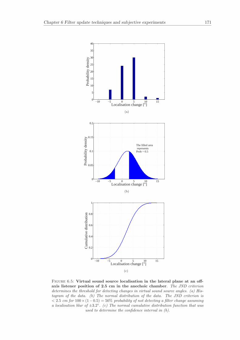
Chapter 6 Filter update techniques and subjective experiments 171
−10 −5 0 5 10 150
5
10
15
20
25
30
35
40
Localisation change [°]
Pro
babi
lity
dens
ity
(a)
−10 −5 0 5 10 150
0.05
0.1
0.15
0.2
The filled area represents Prob = 0.5
Localisation change [°]
Pro
babi
lity
dens
ity
(b)
−10 −5 0 5 10 150
0.2
0.4
0.6
0.8
1
Localisation change [°]
Cum
ulat
ive
dist
ribut
ion
(c)
Figure 6.5: Virtual sound source localisation in the lateral plane at an off-axis listener position of 2.5 cm in the anechoic chamber. The JND criteriondetermines the threshold for detecting changes in virtual sound source angles. (a) His-togram of the data. (b) The normal distribution of the data. The JND criterion is< 2.5 cm for 100× (1−0.5) = 50% probability of not detecting a filter change assuminga localisation blur of ±3.2. (c) The normal cumulative distribution function that was
used to determine the confidence interval in (b).
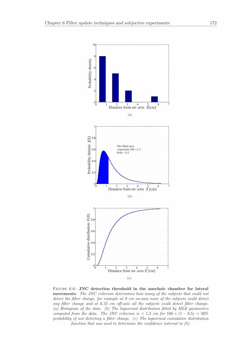
Chapter 6 Filter update techniques and subjective experiments 172
0 1 2 3 4 5 6 70
2
4
6
8
10
Distance from on−axis X[cm]
Pro
babi
lity
dens
ity
(a)
0 1 2 3 4 5 6 70
0.2
0.4
0.6
0.8
1
The filled area represents JNC<1.2Prob = 0.5
Distance from on−axis X [cm]
Pro
babi
lity
dens
ity f(
X)
(b)
0 1 2 3 4 5 6 70
0.2
0.4
0.6
0.8
1
Distance from on−axis X [cm]
Cum
ulat
ive
dist
ribut
ion F
(X)
(c)
Figure 6.6: JNC detection threshold in the anechoic chamber for lateralmovements. The JNC criterion determines how many of the subjects that could notdetect the filter change, for example at 0 cm on-axis none of the subjects could detectany filter change and at 6.25 cm off-axis all the subjects could detect filter change.(a) Histogram of the data. (b) The lognormal distribution fitted by MLE parameterscomputed from the data. The JNC criterion is < 1.2 cm for 100 × (1 − 0.5) = 50%probability of not detecting a filter change. (c) The lognormal cumulative distribution
function that was used to determine the confidence interval in (b).
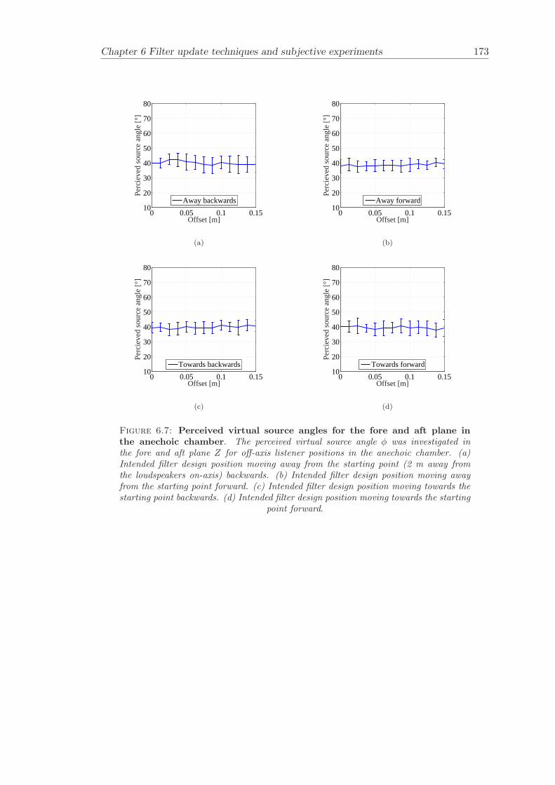
Chapter 6 Filter update techniques and subjective experiments 173
0 0.05 0.1 0.1510
20
30
40
50
60
70
80
Offset [m]
Per
ciev
ed s
ourc
e an
gle
[°]
Away backwards
(a)
0 0.05 0.1 0.1510
20
30
40
50
60
70
80
Offset [m]
Per
ciev
ed s
ourc
e an
gle
[°]
Away forward
(b)
0 0.05 0.1 0.1510
20
30
40
50
60
70
80
Offset [m]
Per
ciev
ed s
ourc
e an
gle
[°]
Towards backwards
(c)
0 0.05 0.1 0.1510
20
30
40
50
60
70
80
Offset [m]
Per
ciev
ed s
ourc
e an
gle
[°]
Towards forward
(d)
Figure 6.7: Perceived virtual source angles for the fore and aft plane inthe anechoic chamber. The perceived virtual source angle φ was investigated inthe fore and aft plane Z for off-axis listener positions in the anechoic chamber. (a)Intended filter design position moving away from the starting point (2 m away fromthe loudspeakers on-axis) backwards. (b) Intended filter design position moving awayfrom the starting point forward. (c) Intended filter design position moving towards thestarting point backwards. (d) Intended filter design position moving towards the starting
point forward.
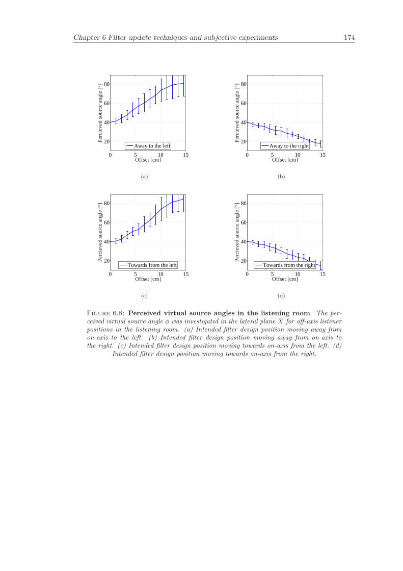
Chapter 6 Filter update techniques and subjective experiments 174
0 5 10 15
20
40
60
80
Offset [cm]
Per
ciev
ed s
ourc
e an
gle
[°]
Away to the left
(a)
0 5 10 15
20
40
60
80
Offset [cm]
Per
ciev
ed s
ourc
e an
gle
[°]
Away to the right
(b)
0 5 10 15
20
40
60
80
Offset [cm]
Per
ciev
ed s
ourc
e an
gle
[°]
Towards from the left
(c)
0 5 10 15
20
40
60
80
Offset [cm]
Per
ciev
ed s
ourc
e an
gle
[°]
Towards from the right
(d)
Figure 6.8: Perceived virtual source angles in the listening room. The per-ceived virtual source angle φ was investigated in the lateral plane X for off-axis listenerpositions in the listening room. (a) Intended filter design position moving away fromon-axis to the left. (b) Intended filter design position moving away from on-axis tothe right. (c) Intended filter design position moving towards on-axis from the left. (d)
Intended filter design position moving towards on-axis from the right.
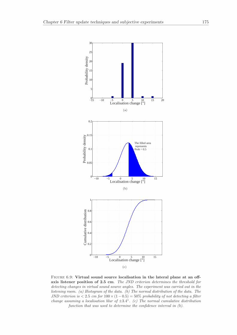
Chapter 6 Filter update techniques and subjective experiments 175
−15 −10 −5 0 5 10 15 200
5
10
15
20
25
30
Localisation change [°]
Pro
babi
lity
dens
ity
(a)
−10 −5 0 5 10 150
0.05
0.1
0.15
0.2
The filled area represents Prob = 0.5
Localisation change [°]
Pro
babi
lity
dens
ity
(b)
−10 −5 0 5 10 150
0.2
0.4
0.6
0.8
1
Localisation change [°]
Cum
ulat
ive
dist
ribut
ion
(c)
Figure 6.9: Virtual sound source localisation in the lateral plane at an off-axis listener position of 2.5 cm. The JND criterion determines the threshold fordetecting changes in virtual sound source angles. The experiment was carried out in thelistening room. (a) Histogram of the data. (b) The normal distribution of the data. TheJND criterion is < 2.5 cm for 100× (1− 0.5) = 50% probability of not detecting a filterchange assuming a localisation blur of ±3.4. (c) The normal cumulative distribution
function that was used to determine the confidence interval in (b).
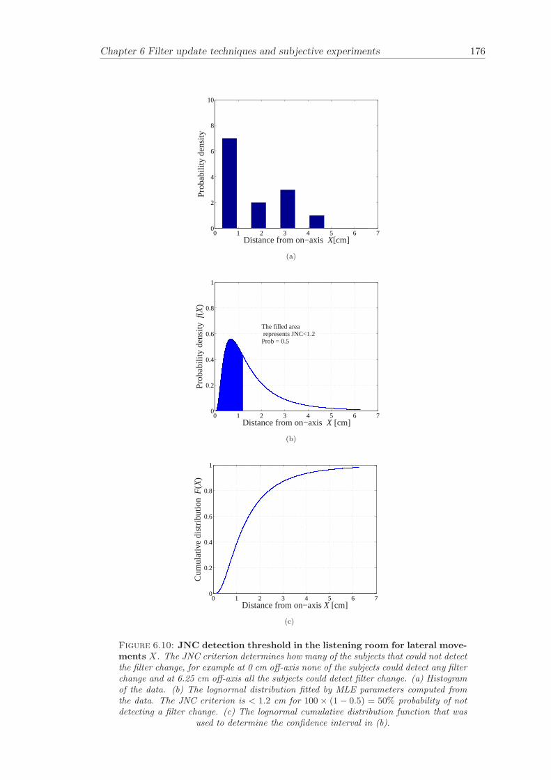
Chapter 6 Filter update techniques and subjective experiments 176
0 1 2 3 4 5 6 70
2
4
6
8
10
Distance from on−axis X[cm]
Pro
babi
lity
dens
ity
(a)
0 1 2 3 4 5 6 70
0.2
0.4
0.6
0.8
1
The filled area represents JNC<1.2Prob = 0.5
Distance from on−axis X [cm]
Pro
babi
lity
dens
ity f(
X)
(b)
0 1 2 3 4 5 6 70
0.2
0.4
0.6
0.8
1
Distance from on−axis X [cm]
Cum
ulat
ive
dist
ribut
ion F
(X)
(c)
Figure 6.10: JNC detection threshold in the listening room for lateral move-ments X. The JNC criterion determines how many of the subjects that could not detectthe filter change, for example at 0 cm off-axis none of the subjects could detect any filterchange and at 6.25 cm off-axis all the subjects could detect filter change. (a) Histogramof the data. (b) The lognormal distribution fitted by MLE parameters computed fromthe data. The JNC criterion is < 1.2 cm for 100 × (1 − 0.5) = 50% probability of notdetecting a filter change. (c) The lognormal cumulative distribution function that was
used to determine the confidence interval in (b).
Chapter 7
Image processing algorithms for
listener head tracking
There is a demand for a head-tracking algorithm, because of the relatively small “sweet-spot” size of loudspeaker based binaural sound reproduction systems. Adding access toa video camera for the audio system gives the possibility to track head movements andupdate the inverse filters accordingly. There are several alternative methods for headtracking, such as, magnetic, infrared and laser tracking, though they typically requiresensors to be worn by the user or are expensive. Visual tracking has emerged as one ofthe principal areas of research within the computer vision community. The increasinginterest in visual tracking is due in part to the falling cost of computing power, videocameras and memory. A sequence of images grabbed at or near video rate typicallydoes not change radically from frame to frame, and this redundancy of information overmultiple images can be extremely helpful for analysing the input to track individualobjects. The ideal algorithm for this application should be robust to background noise,track the position of the head (and ears) and be computationally efficient.
Preliminary work on this topic has been carried out at ISVR and has been based onvery simple template matching algorithms that capture an image of the listener’s headand then ensure a best estimate of the listener head position by finding the templateposition that best matches the current image. It is important that the image processingalgorithms used are efficient in order to make the processing required as small as possible.A literature survey has been carried out in order to provide an initial evaluation of thecandidate algorithms currently available.
There are many approaches possible for head tracking. Jones [42] concludes that it ispossible to build powerful generic models for low-level image attributes like colour usingsimple histogram learning techniques. They describe the construction of colour modelsfor skin and non-skin classes from a huge dataset of nearly 1 billion labelled pixels. Theseclasses are found to exhibit a surprising degree of separability which can be exploited
177
Chapter 7 Image processing algorithms for listener head tracking 178
by building a skin pixel detector achieving a detection rate of 80% with 8.5% falsepositives. Bowden [15] demonstrates how to use red green blue (RGB) colour spaces toprobabilistically label and segment regions of skin from image sequences for the locationand tracking of the human face. He has also demonstrated that human skin clusters ina small region of colour space, since human skin colours differ more in intensity thanactual colour, and under certain lighting conditions, a skin colour distribution can becharacterised by a multivariate Gaussian distribution in a normalised colour space. Theuse of colour labelling can provide a rough estimate of the location of a head within theimage frame to initialise a listener head tracking system and to track the translation ofthe listener in the following frames.
The distance cue for the listener can be found by using stereo area correlation tracking.Stereo analysis is the process of measuring the distance to an object based on a compar-ison of the object projection of two images. The stereo analysis technique developed byKonolige [53] uses area correlation to compare small patches among images. Stereo areacorrelation is a reliable technique for finding distance information in images. Stereo areacorrelation can be used to track people in natural environments by applying backgroundsubtraction and segmentation of the image with distance information. The major dis-advantage with this tracking scheme is the background subtraction step, which is notdesirable to carry out. Since, the background is changing frequently in most listeningenvironments it would become a problem to calibrate the system.
Contours in images can be used for detecting the position and shape of objects. Theoriginal “snake” model was introduced by Kass [46] and this concept has been furtherdeveloped by authors such as Gunn [34], [35]. The technique presented by Gunn canbe used find the position and shape of the head. However, it is relatively sensitive tothe quality of edge detection and the factors affecting this, namely illumination andboundary contrast. Blake [12] and Isard [41] established a stochastic framework fortracking curves in visual clutter using a Bayesian random sampling algorithm. Thetask was to track outlines and features of foreground objects, modelled as curves in acluttered background. The curve models are named deformable contours, also knownas “active contours” or “snakes”. A particle filtering technique named the “condensa-tion algorithm” was used for tracking objects described by contours in highly clutteredenvironments. The main disadvantage of using the condensation algorithm is its com-putational inefficiency.
7.1 Overview of object localisation techniques
Much has been written about object localisation, and this section attempts to summarisethe approaches used by previous researchers in computer vision. Table 7.1 gives anoverview of approaches for detecting the position and shape of rigid objects. The table
Chapter 7 Image processing algorithms for listener head tracking 179
can used as a rough guide in choosing an appropriate approach for solving an objectlocalisation problem. The algorithms for tracking objects in images can be dividedinto three types namely “global matching”, “pose space search” and “correspondencespace search” (Grimson [33]). The global matching approach to object localisationinvolves finding a transformation from a model to an image without determining thecorrespondence linking individual features of the model and the data. Here global refersto features or parameters that depend on the whole object, for example, area or volume.The usual approach is to compute a group of global parameters of a model and of thesensory data represented as a vector of parameters. An example of global parametermatching is to produce a binary image where each pixel with a value of 1 represents theobject and the background pixels are set to 0. This can be achieved, for example, bythresholding an intensity image F.
F(x, y) =
1 object pixel
0 otherwise(7.1)
(7.2)
where the index x denotes the horizontal axis in the image and index y denotes thevertical axis of the image. Then the moments of each model is computed and comparedto the moments of the binary image. For example, the zeroth order moment is given by
A =∑
x
∑y
F(x, y) (7.3)
that computes the area of the object. Higher order moments are defined as
Mp,q =∑
x
∑y
xpyqF(x, y) (7.4)
where the first moments gives the centre of mass (position) of the object. The skincolour tracking approach in Section 7.2 is another example of global matching.
The searching of correspondence space involves focusing on the matching process. Con-sider an object model represented by a group of features, each with an individual labelthat is associated with a set of attributes. Likewise, the sensory data results in a groupof features with individual labels that are associated with a set of attributes. Then thesearch problem can be solved by considering the space of all possible matches of datafeatures to model features. Given that there are d sensory data features and m modelfeatures, then we can imagine a d-dimensional space, along each axis of which there arem + 1 (+1 is due to the event of false detection) discrete possible values. Each point in
Chapter 7 Image processing algorithms for listener head tracking 180
correspondence space represents an interpretation of all of the data points. There are(m+1)d nodes in this space, which is highly computational demanding in most applica-tions, therefore various techniques for imposing constraints on the correspondence spacehave been investigated by previous researchers (Grimson [33]).
The pose space search involves the evaluation of possible transformations of the modelinto the data. Unlike the correspondence space search that finds the association of datafeatures and model features, while the pose of the object is of secondary importance.The pose space search focuses on finding poses of an object model that is imposed onto the sensory data. The pose space search can be represented by, for example a three-dimensional space having two axes for translational components and one for rotation.Then each point in the configuration of pose space corresponds to a different pose of themodel and the idea is to determine which poses that best fit the data. This approach isfurther described in Section 7.4.
Many techniques for object localisation have concentrated on searching a correspondencespace. The number of detected features can become large, which means that they haveto be limited in some way. For example, probabilistic reasoning can be used to limitthe number of features. However, the disadvantage of this approach is that the targetneed have easily detectable features, such as corners or colour, and detailed models ofthe target need to be known. In some cases, such as here where the target is a face,there are relatively easily detectable features. The features that are feasible to detectin face include skin colour, eyes and nose. The main advantage of this approach isthe computational efficiency that can be achieved when the target features are easilydetectable.
Correlation based techniques are fundamentally based on correlating a known templatewith various regions in an image and can be run effectively in hardware. However,in general the pose space needs to be of a very small dimension. Contour trackingusing a particle filter is also a pose space search, which also requires the dimension ofthis space to be small. Experiments show that if the prior is diffuse over more thanthree or four dimensions, then the algorithm tends to be to slow for real time tracking(MacCormick [62]). The advantages are that it can be applied for a wide range of objectswith minimal modelling requirements and it is very insensitive to cluttered environments.
Other techniques for feature detection include the Hough transform that is a well-knowntechnique for localising corners and lines in images. The Hough transform can for exam-ple be used to detect the corners of the eyes in a face. Optical flow is another methodfor target localisation. However, it requires the target to move and the camera and thebackground to be fixed. The background subtraction step is surprisingly sensitive tocamera movements and lighting changes.
A series of computer simulation studies have been undertaken in order to evaluatepromising candidate algorithms, especially with regard to computational efficiency and

Chapter 7 Image processing algorithms for listener head tracking 181
Techniques Advantages Disadvantages ExamplesGlobal Image * Faster than * Objects need Grimson [33];matching segmentation pose space to be separated this chapter
(blobs etc.) and from backgroundcorrespondence * Light sensitivespace
Correspondence Feature * Faster than * Objects need Grimson [33]space search detection pose space to have clearly
search (of high detectabledimension) features
Pose space Correlation * Technology * Light sensitive Ballard [8];search ready available * Can not handle Cootes [22]
irregular shapesContour * Simplified * Not suitable Blake [12];tracking modelling for complex this chapterusing particle of targets 3D structuresfilters * Clutter * Occasional
resistance false detectionOther Hough transform * Effective * Limited for Duda [26]
when applicable other shapesthan cornersand lines
Optical flow * Simple * Requires moving Subbarao [94]geometric target andmodelling fixed background
Table 7.1: Approaches for detecting the position and shape of objects.
clutter resistance. The algorithms that have been evaluated for listener head trackingare colour tracking (of skin), stereo area correlation and contour tracking. The colourtracking algorithm evaluated here is based on statistical colour distribution in Red GreenBlue (RGB) space and is presented in Section 7.2. The colour tracking algorithm findsthe skin region in an image that represents the face of the listener and tracks listenertranslation. The main advantage of this relatively simple algorithm is that it can berun efficiently on available hardware. The presented stereo area correlation algorithmrequires two cameras and is described in Section 7.3. The stereo algorithm calculatesthe distance of the objects in the camera field and hence the distance to the listener.The stereo area correlation technique is a well known algorithm that can find distanceinformation in image sequences in real time. The contour tracking algorithm makes itpossible to track the listener in an affine “shape space” of six DOF and is presented inSection 7.4. The contour tracking approach was investigated to improve the robustnessof tracking through serious clutter and changes in illumination. The visual trackingsystem is implemented by using a stereo camera package (Small Vision System (SVS)).
Chapter 7 Image processing algorithms for listener head tracking 182
7.2 Colour tracking
The colour content of an image is an important attribute. This section will discuss howcolour can be used to provide a reliable feature for locating and tracking moving objects.The availability of colour generally provides a more distinguishable difference betweenforeground and background objects within an image. Cambridge research laboratoryin Massachusetts (Jones [42]) has used large image data sets of photos on the WorldWide Web to build powerful generic models from colour using histogram learning tech-niques and multivariate Gaussian classifiers. They have demonstrated that human skinclusters in a relatively small region of colour space. A skin colour distribution can becharacterised by a multivariate Gaussian distribution in a colour space as previously in-vestigated by Bowden [15], Jones [42], Azarbayejani [6], [7] and Kuchi [55]. This colourlabelling can be used to provide an estimate of the location of a head within the imageframe to initialise a head tracking system and also to use the colour feature for tracking.
By performing image processing upon a greyscale representation, calculated from thecolour channels (typically the average intensity of the three colour channels) a consid-erable amount of information about object boundaries is lost. An RGB image thatconsists of three colour regions where each region has the same intensity in its colourchannel for example: the red area has R = 255, G = 0, and B = 0; the green area hasR = 0, G = 255 and B = 0; etc. By taking the average of the three colour channels ateach pixel, the resulting image would have a constant intensity of 85 and no distinctionwould be possible between the various areas. However, in the colour image, it is visuallyapparent that such a distinction does exist and very clear boundaries are defined. It isclear that reducing colour information to one channel “throws information away”, whichmay be invaluable to the application at hand. If an object of interest is sufficientlyprominent within one of the colour channels, then the intensity of that channel can beused instead of the mean intensity.
7.2.1 Multivariate Gaussian probability distribution
The colour representation of a face in a video sequence is influenced by many factorssuch as ambient light and the object moving relative to a light source. Also humanskin colours deviate in RGB space from person to person, although they still cluster in arelatively small space (Bowden [15]). When the skin colour of the person is known a priorithen colour can be used as a robust feature for tracking skin colour in a video sequencewith consistent ambient light. The skin colour of a subject head can be extracted byselecting a “training set” of skin pixels in the image. The training set of skin pixelswas here chosen on a frame from the image sequence used in the tracking experiment inSection 7.2.2.
The set of pixels that constitute the foreground with skin pixels is denoted X ∈ F
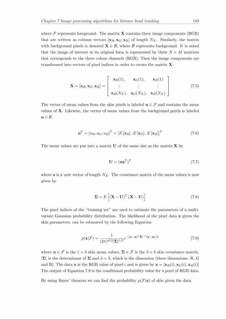
Chapter 7 Image processing algorithms for listener head tracking 183
where F represents foreground. The matrix X contains three image components (RGB)that are written as column vectors [xR,xG,xB] of length NX . Similarly, the matrixwith background pixels is denoted X ∈ B, where B represents background. It is notedthat the image of interest in its original form is represented by three N ×M matricesthat corresponds to the three colour channels (RGB). Then the image components aretransformed into vectors of pixel indices in order to create the matrix X.
X = [xR,xG,xB] =
xR(1), xG(1), xB(1)...
......
xR(NX), xG(NX), xB(NX)
(7.5)
The vector of mean values from the skin pixels is labeled u ∈ F and contains the meanvalues of X. Likewise, the vector of mean values from the background pixels is labeledu ∈ B.
uT = [uR, uG, uB]T = [E [xR] , E [xG] , E [xB]]T (7.6)
The mean values are put into a matrix U of the same size as the matrix X by
U = (uzT )T (7.7)
where z is a unit vector of length NX . The covariance matrix of the mean values is nowgiven by
Σ = E[(X−U)T (X−U)
](7.8)
The pixel indices of the “training set” are used to estimate the parameters of a multi-variate Gaussian probability distribution. The likelihood of the pixel data x given theskin parameters, can be estimated by the following Equation
p(x|F) =1
(2π)d/2|Σ|1/2e−(x−u)T Σ−1(x−u)/2 (7.9)
where u ∈ F is the 1× 3 skin mean values, Σ ∈ F is the 3× 3 skin covariance matrix,|Σ| is the determinant of Σ and d = 3, which is the dimension (three dimensions: R, Gand B). The data x is the RGB value of pixel i and is given by x = [xR(i),xG(i),xB(i)]The output of Equation 7.9 is the conditional probability value for a pixel of RGB data.
By using Bayes’ theorem we can find the probability p(F|x) of skin given the data.
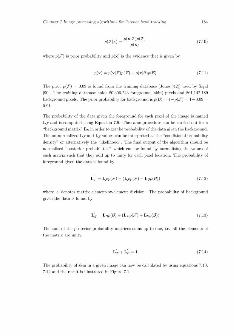
Chapter 7 Image processing algorithms for listener head tracking 184
p(F|x) =p(x|F)p(F)
p(x)(7.10)
where p(F) is prior probability and p(x) is the evidence that is given by
p(x) = p(x|F)p(F) + p(x|B)p(B) (7.11)
The prior p(F) = 0.09 is found from the training database (Jones [42]) used by Sigal[90]. The training database holds 80,306,243 foreground (skin) pixels and 861,142,189background pixels. The prior probability for background is p(B) = 1−p(F) = 1−0.09 =0.91.
The probability of the data given the foreground for each pixel of the image is namedLF and is computed using Equation 7.9. The same procedure can be carried out for a“background matrix” LB in order to get the probability of the data given the background.The un-normalized LF and LB values can be interpreted as the “conditional probabilitydensity” or alternatively the “likelihood”. The final output of the algorithm should benormalised “posterior probabilities” which can be found by normalising the values ofeach matrix such that they add up to unity for each pixel location. The probability offoreground given the data is found by
L′F = LFp(F)÷ (LFp(F) + LBp(B)) (7.12)
where ÷ denotes matrix element-by-element division. The probability of backgroundgiven the data is found by
L′B = LBp(B)÷ (LFp(F) + LBp(B)) (7.13)
The sum of the posterior probability matrices sums up to one, i.e. all the elements ofthe matrix are unity.
L′F + L
′B = 1 (7.14)
The probability of skin in a given image can now be calculated by using equations 7.10,7.12 and the result is illustrated in Figure 7.1.
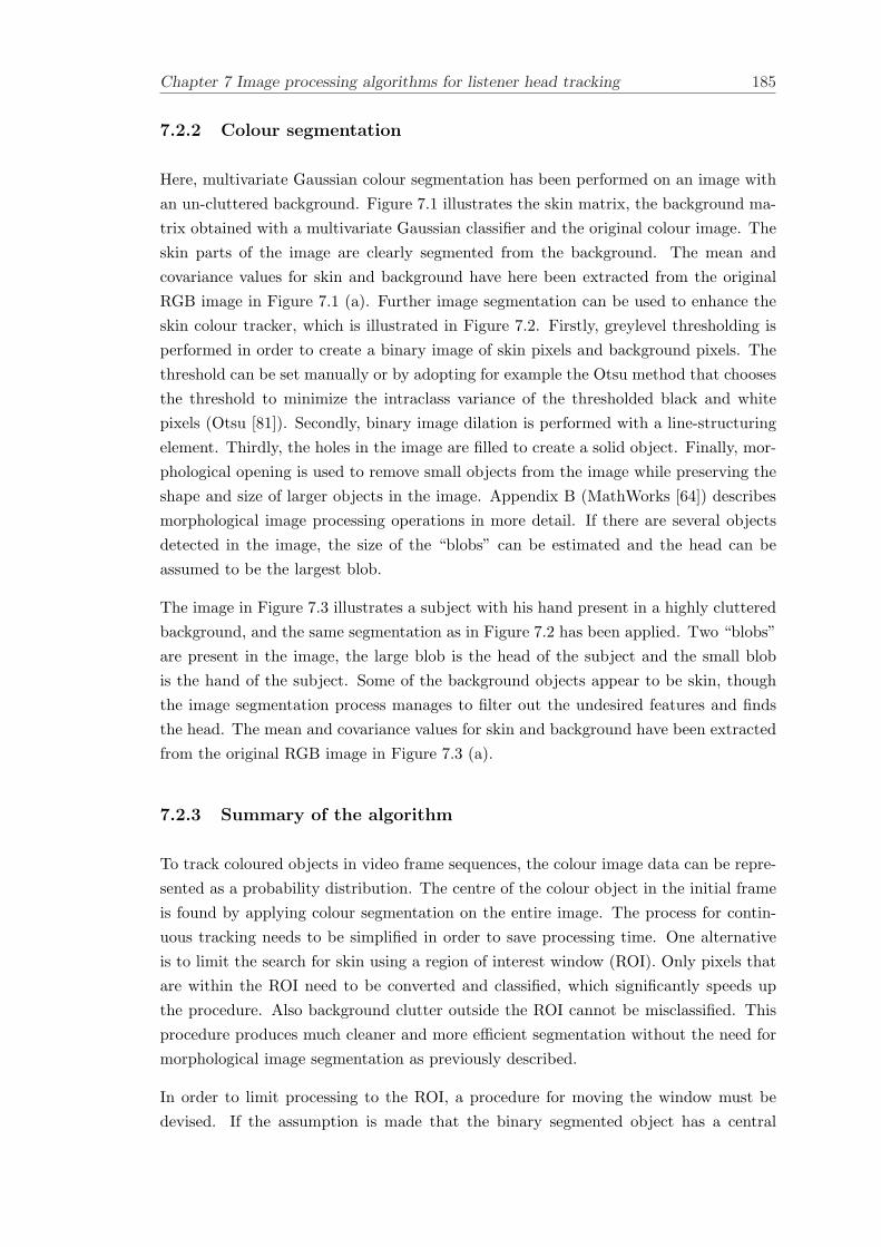
Chapter 7 Image processing algorithms for listener head tracking 185
7.2.2 Colour segmentation
Here, multivariate Gaussian colour segmentation has been performed on an image withan un-cluttered background. Figure 7.1 illustrates the skin matrix, the background ma-trix obtained with a multivariate Gaussian classifier and the original colour image. Theskin parts of the image are clearly segmented from the background. The mean andcovariance values for skin and background have here been extracted from the originalRGB image in Figure 7.1 (a). Further image segmentation can be used to enhance theskin colour tracker, which is illustrated in Figure 7.2. Firstly, greylevel thresholding isperformed in order to create a binary image of skin pixels and background pixels. Thethreshold can be set manually or by adopting for example the Otsu method that choosesthe threshold to minimize the intraclass variance of the thresholded black and whitepixels (Otsu [81]). Secondly, binary image dilation is performed with a line-structuringelement. Thirdly, the holes in the image are filled to create a solid object. Finally, mor-phological opening is used to remove small objects from the image while preserving theshape and size of larger objects in the image. Appendix B (MathWorks [64]) describesmorphological image processing operations in more detail. If there are several objectsdetected in the image, the size of the “blobs” can be estimated and the head can beassumed to be the largest blob.
The image in Figure 7.3 illustrates a subject with his hand present in a highly clutteredbackground, and the same segmentation as in Figure 7.2 has been applied. Two “blobs”are present in the image, the large blob is the head of the subject and the small blobis the hand of the subject. Some of the background objects appear to be skin, thoughthe image segmentation process manages to filter out the undesired features and findsthe head. The mean and covariance values for skin and background have been extractedfrom the original RGB image in Figure 7.3 (a).
7.2.3 Summary of the algorithm
To track coloured objects in video frame sequences, the colour image data can be repre-sented as a probability distribution. The centre of the colour object in the initial frameis found by applying colour segmentation on the entire image. The process for contin-uous tracking needs to be simplified in order to save processing time. One alternativeis to limit the search for skin using a region of interest window (ROI). Only pixels thatare within the ROI need to be converted and classified, which significantly speeds upthe procedure. Also background clutter outside the ROI cannot be misclassified. Thisprocedure produces much cleaner and more efficient segmentation without the need formorphological image segmentation as previously described.
In order to limit processing to the ROI, a procedure for moving the window must bedevised. If the assumption is made that the binary segmented object has a central

Chapter 7 Image processing algorithms for listener head tracking 186
white mass surrounded by black background, then the centre of the “blob” should be atthe centre of the window. A simple translation can then be calculated to position thecentre of the window at the centre of the segmented feature for the next iteration of thealgorithm. The size of the window can be configured to be 10% larger than the “blob”that represents the head.
Figure 7.4 illustrates the probability of skin in the first frame of an image sequence.The ROI has been determined by performing morphological image segmentation and itfits closely to the head. A threshold is configured for the skin pixel probabilities in theROI in order to get a binary image with skin and not skin pixels. The binary imageis calculated with a simple algorithm that searches every pixel in the ROI and sets thepixel to zero if the pixel value is less then the threshold and sets the pixel to one if thepixel value is greater then the threshold. The threshold level can be found by usingReceiver Operating Characteristics (ROC) (Sigal [90]) or by experiment.
The following provides a summary of the algorithm:
(1) Initialisation
(1.1) Construct a multivariate probability function for skin and background with Equa-tion 7.9. Calculate the probability of the data x given skin for each pixel in the inputimage. Compute the probability of skin given x by using Bayes’ theorem Equation 7.12.
(1.2) Perform morphological image segmentation as illustrated in Figure 7.2. The outputimage obtained is a binary image of skin pixels and non-skin pixels.
(1.3) Search the output image for the largest “blob”.
(1.4) Calculate the centre of the largest “blob” and initialise the window to this position.
(2) Tracking
(2.1) Calculate the size of the largest “blob” and make the window approximately 10%larger.
(2.2) Capture the new input image.
(2.3) Segment the image in the window using the probability density function as in point(1.1). The priors in the ROI are estimated to be approximately equal p(F ) = p(B) = 0.5.Then threshold the probabilities map in order to obtain the output image, which is abinary image of skin pixels and not skin pixels (see Figure 7.4).
(2.4) Calculate the mean white pixel in order to find the centre.
(2.5) Move the window to the centre.
(2.6) Enlarge the window by a suitable number of pixels; here 5 pixels have been provento work well. Then repeat steps (2.3), (2.4) and (2.5) again and then fit a new window
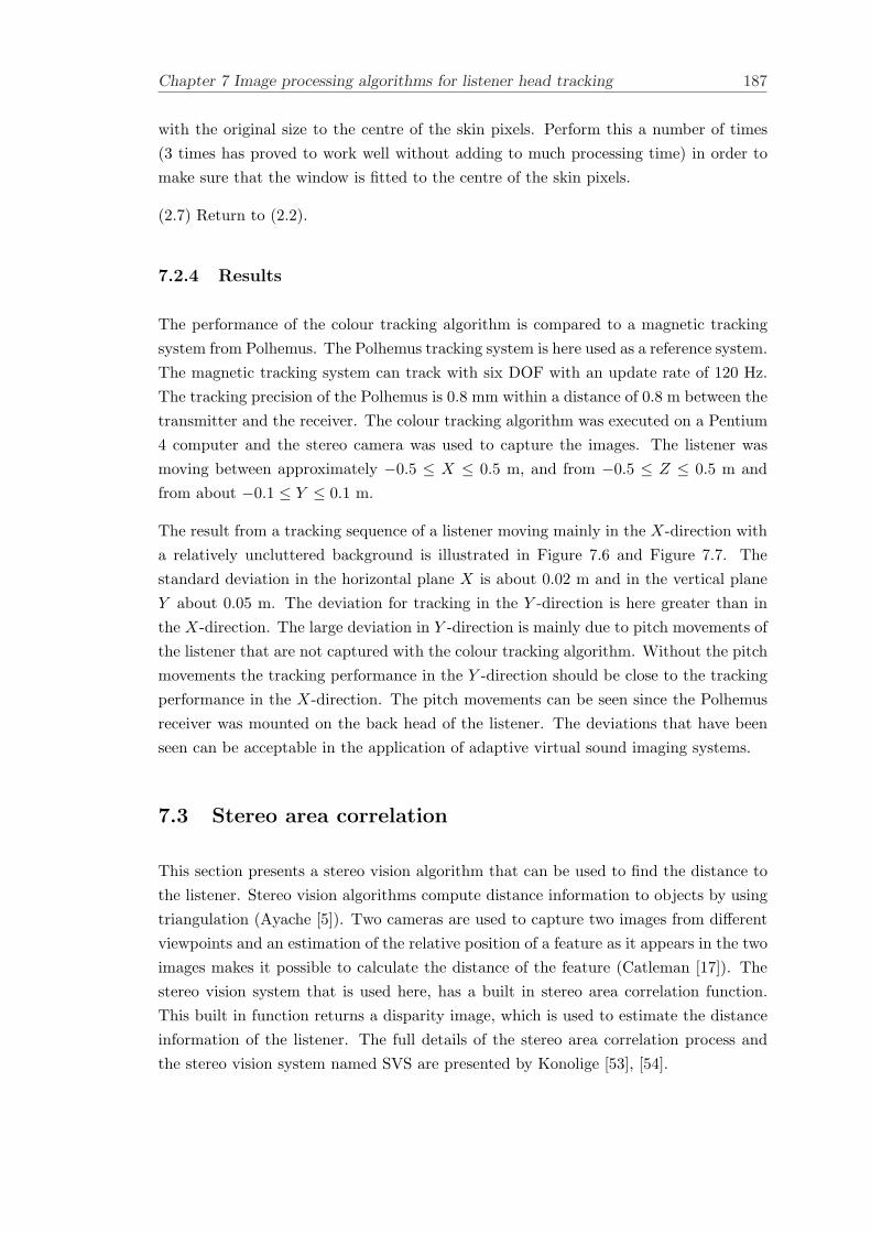
Chapter 7 Image processing algorithms for listener head tracking 187
with the original size to the centre of the skin pixels. Perform this a number of times(3 times has proved to work well without adding to much processing time) in order tomake sure that the window is fitted to the centre of the skin pixels.
(2.7) Return to (2.2).
7.2.4 Results
The performance of the colour tracking algorithm is compared to a magnetic trackingsystem from Polhemus. The Polhemus tracking system is here used as a reference system.The magnetic tracking system can track with six DOF with an update rate of 120 Hz.The tracking precision of the Polhemus is 0.8 mm within a distance of 0.8 m between thetransmitter and the receiver. The colour tracking algorithm was executed on a Pentium4 computer and the stereo camera was used to capture the images. The listener wasmoving between approximately −0.5 ≤ X ≤ 0.5 m, and from −0.5 ≤ Z ≤ 0.5 m andfrom about −0.1 ≤ Y ≤ 0.1 m.
The result from a tracking sequence of a listener moving mainly in the X-direction witha relatively uncluttered background is illustrated in Figure 7.6 and Figure 7.7. Thestandard deviation in the horizontal plane X is about 0.02 m and in the vertical planeY about 0.05 m. The deviation for tracking in the Y -direction is here greater than inthe X-direction. The large deviation in Y -direction is mainly due to pitch movements ofthe listener that are not captured with the colour tracking algorithm. Without the pitchmovements the tracking performance in the Y -direction should be close to the trackingperformance in the X-direction. The pitch movements can be seen since the Polhemusreceiver was mounted on the back head of the listener. The deviations that have beenseen can be acceptable in the application of adaptive virtual sound imaging systems.
7.3 Stereo area correlation
This section presents a stereo vision algorithm that can be used to find the distance tothe listener. Stereo vision algorithms compute distance information to objects by usingtriangulation (Ayache [5]). Two cameras are used to capture two images from differentviewpoints and an estimation of the relative position of a feature as it appears in the twoimages makes it possible to calculate the distance of the feature (Catleman [17]). Thestereo vision system that is used here, has a built in stereo area correlation function.This built in function returns a disparity image, which is used to estimate the distanceinformation of the listener. The full details of the stereo area correlation process andthe stereo vision system named SVS are presented by Konolige [53], [54].

Chapter 7 Image processing algorithms for listener head tracking 188
7.3.1 Stereo analysis
Stereo analysis is the process of measuring distance to an object based on a comparisonof the object projection on two or more images. The problem to be solved is to findcorresponding elements between the images and once a match is made, then the distanceto the object can be computed using the image geometry as described in Appendix B.The common method for stereo analysis is to use area correlation, which compares smallpatches or windows among images using correlation. The window size will always be acompromise, since small windows are more likely to be similar in images with differentviewpoints, and large windows increase the signal to noise ratio.
In Figure 7.8 area correlation and the pixel-shift calculation is illustrated. The stationarywindow is chosen to be in the left image and hence the moving window in the rightwindow. For each pixel, the area correlation is calculated by moving the window in theright image. The area correlation is calculated by the Laplacian of Gaussian (LOG)transform and L1 norm (absolute difference). The LOG transform measures directededge intensities over the area smoothed by the Gaussian. The LOG transform and L1norm have proven to give good results (Konolige [54]).
7.3.2 Summary of the algorithm
A brief summary of the stereo area correlation algorithm is presented here. The stereoarea correlation algorithm can be divided into five steps as follows
(1) Geometry correction: distortions in the input images are corrected.
(2) Image transform: a local operator transforms each pixel in the greyscale image intoa more appropriate form, e.g., normalizes it based on average local intensity.
(3) Area correlation: each small area is compared with other areas in its search window.The area correlation is calculated by the Laplacian of Gaussian (LOG) transform andL1 norm (absolute difference).
(4) Extrema extraction: the extreme value of the correlation at each pixel is determined,which results in a disparity image. The disparity measure is further described in Ap-pendix B. In the disparity image, each pixel value is the disparity between left and rightimage patches at the best match.
(5) Post-filtering: Interest operator and left/right check filters are applied in order toclean up noise in the disparity image.
The stereo area correlation algorithm performs the five steps above for each frame andthe result is a disparity image of each frame (Konolige [54]).
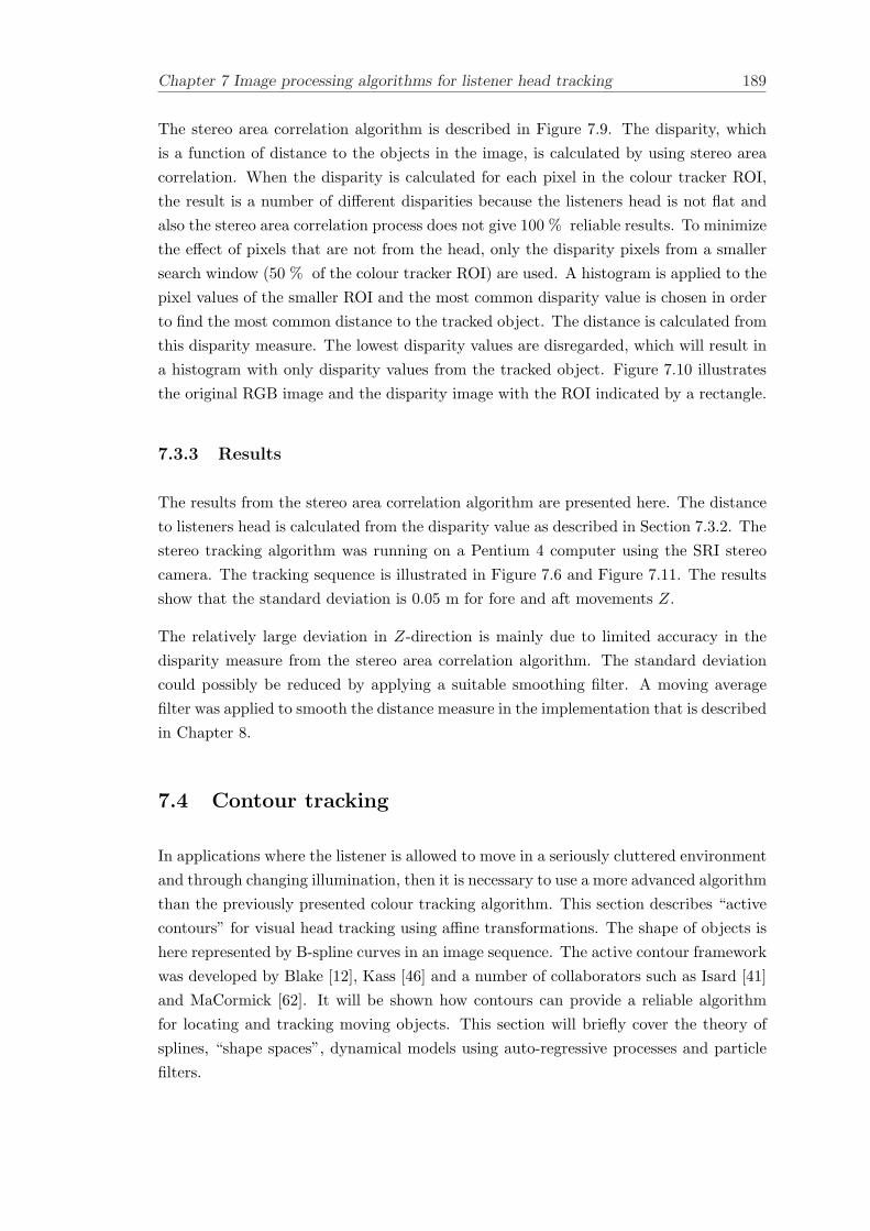
Chapter 7 Image processing algorithms for listener head tracking 189
The stereo area correlation algorithm is described in Figure 7.9. The disparity, whichis a function of distance to the objects in the image, is calculated by using stereo areacorrelation. When the disparity is calculated for each pixel in the colour tracker ROI,the result is a number of different disparities because the listeners head is not flat andalso the stereo area correlation process does not give 100 % reliable results. To minimizethe effect of pixels that are not from the head, only the disparity pixels from a smallersearch window (50 % of the colour tracker ROI) are used. A histogram is applied to thepixel values of the smaller ROI and the most common disparity value is chosen in orderto find the most common distance to the tracked object. The distance is calculated fromthis disparity measure. The lowest disparity values are disregarded, which will result ina histogram with only disparity values from the tracked object. Figure 7.10 illustratesthe original RGB image and the disparity image with the ROI indicated by a rectangle.
7.3.3 Results
The results from the stereo area correlation algorithm are presented here. The distanceto listeners head is calculated from the disparity value as described in Section 7.3.2. Thestereo tracking algorithm was running on a Pentium 4 computer using the SRI stereocamera. The tracking sequence is illustrated in Figure 7.6 and Figure 7.11. The resultsshow that the standard deviation is 0.05 m for fore and aft movements Z.
The relatively large deviation in Z-direction is mainly due to limited accuracy in thedisparity measure from the stereo area correlation algorithm. The standard deviationcould possibly be reduced by applying a suitable smoothing filter. A moving averagefilter was applied to smooth the distance measure in the implementation that is describedin Chapter 8.
7.4 Contour tracking
In applications where the listener is allowed to move in a seriously cluttered environmentand through changing illumination, then it is necessary to use a more advanced algorithmthan the previously presented colour tracking algorithm. This section describes “activecontours” for visual head tracking using affine transformations. The shape of objects ishere represented by B-spline curves in an image sequence. The active contour frameworkwas developed by Blake [12], Kass [46] and a number of collaborators such as Isard [41]and MaCormick [62]. It will be shown how contours can provide a reliable algorithmfor locating and tracking moving objects. This section will briefly cover the theory ofsplines, “shape spaces”, dynamical models using auto-regressive processes and particlefilters.
Chapter 7 Image processing algorithms for listener head tracking 190
7.4.1 Spline curves
Visual curves can be represented in terms of parametric spline curves, which is commonin computer graphics. The parametric spline curves are used because they can efficientlyrepresent sets of boundary curves in an image. This section forms the basis for contourtracking. The curves are denoted, r(s) = (x(s), y(s)) where s is a parameter thatincreases as the curve is traversed, and x and y are functions of s known as splines. Theparameterised curve can be written as:
r(s) = (b(s)qx,b(s)qy) for 0 ≤ s ≤ L (7.15)
where b(s) is a vector (b0(s), ..., bNB−1(s))T of B-spline basis functions, qx and qy arevectors of B-spline control point coordinates and L is the number of spans (concatenatedpolynomial segments as described by Blake [12]). For example, the elements of qx definethe x-coordinates of the control points. To simplify the notation, the B-spline controlpoints can be combined in to a spline matrix.
Q =
(qx
qy
)(7.16)
Thus equation 7.15 can be written in matrix form as
r(s) = U(s)Q for 0 ≤ s ≤ L (7.17)
Where the following definition holds
U(s) = I2 ⊗ b(s)T =
(b(s)T 0
0 b(s)T
)(7.18)
and U(s) a matrix of size 2× 2NQ. In this expression ⊗ denotes “Kronecker product”of two matrices and Im denotes an m ×m identity matrix. An example of a quadratic(d = 3), parametric spline curve r(s) is illustrated in Figure 7.12.
7.4.2 Shape space models
The “shape space” is introduced to reduce the dimension. Arbitrary manipulation ofthe spline vectors Q is often too general in practice, therefore a restricted class oftransformations is introduced that is parameterised by a lower dimensional configurationvector y termed a shape space vector. Typical objects require 5 - 20 control points
Chapter 7 Image processing algorithms for listener head tracking 191
to produce a contour that for a human observer, appears to match the object closely(Blake [12]). The vector space of such contours has 10 - 40 dimensions, which is oftenundesirably large. Therefore we work in a vector subspace of <2n termed the shapespace and denoted S. An element y ∈ S is related to the control point coordinates by
Q = Wy + Q0 (7.19)
where W is a NQ×NY “shape matrix”. Q0 is called a constant offset, which is a templatecurve against which shape variations are measured. The shape matrix corresponds to,for example, translation, Euclidian similarities or affine transformation.
The planar affine “shape space” is adopted in this thesis, since it can represent six DOF,to a good approximation, which sufficient for the virtual sound imaging system underinvestigation. The figure below illustrates how a template can be translated, scaled androtated in the planar affine shape space representation.
The “shape matrix” used here is given by
W =
(1 00 1
qx0 00 qy
0
0 qy0
qx0 0
)(7.20)
The first two columns of W represent horizontal and vertical translation. The remain-ing four affine motions can be expressed as simple linear combinations of the four lastcolumns of W.
Some examples of transformations are given below.
1. y = (0, 0, 0, 0, 0, 0)T represents the original template Q0.2. y = (10, 0, 0, 0, 0, 0)T represents the original template translated 10 units to theright.3. y = (0, 0, 1, 1, 0, 0)T represents the original template doubled in size.4. y = (0, 0, cos(θ)− 1, cos(θ)− 1,− sin(θ), sin(θ))T represents the original templaterotated with an angle θ.
7.4.3 Feature detection
This paragraph describes the process of feature detection and introduces the conceptof a limited search region. Feature detection processes are effective up to a point butcannot retrieve entire geometric structures. “Snakes” were therefore introduced by Kass[46] to deal with these limitations of low-level processing. The idea is to take a featuremap F (an image that is processed in order to enhance certain features) such as thatin Figure 7.13 and to treat F as a landscape on which a deformable curve (snake) r(s)
Chapter 7 Image processing algorithms for listener head tracking 192
can slide. For efficiency, the deformable templates described in this section are driventowards a distinguished feature curve rf (s) instead of over the entire image landscapeF that is used in the original snake model.
To reduce the computational cost of applying filters across the entire image, one candefine a search region, in which the corresponding image feature is likely to lie. Thesearch region is defined from an estimate of the position of a tracked image contour.Image processing can now effectively be restricted to this search region as illustrated inFigure 7.14.
The normals to r(s) are constructed at points s = si, i = 1, , N along the curve r(s),which will result in a sequence of sampled points rf (si) i = 1, , N along the featurecurve rf (s). The sample points can be spaced arbitrarily along the curve, for exampleit may be desirable to concentrate the sample points in regions where measurements areexpected to be particularly informative. In reality several features might be detectedon each normal, particularly when tracking in cluttered images. In Section 7.4.5 it isdescribed how to choose the desired features by using the condensation algorithm.
In Figure 7.15, a contour is initialised to the centre of a head (found by using colourtracking) and the result from the feature detection process (using edge detection) isillustrated. At fixed points along the B-spline so called measurement lines, which arenormal to the contour, are introduced onto the image. The length of the measurementlines has been fixed in advance and it is symmetric about the measurement point. Thenext step is to apply a one dimensional feature detector. The edge detector is applied tothe image intensity along each measurement line. The edges are located by applying anoperator mask c(n), −Nc ≤ n ≤ Nc , by discrete convolution, to the samples of themeasurement line f(n), 1 ≤ n ≤ Nf , in order to find the strength of the edges
e(n) =Nc∑
m=−Nc
c(m)f(n + m) (7.21)
The result for each line is a list of numbers describing the distance from each feature tothe measurement point. The two highest values of e(n) are located and the point that isclosest to the previously detected edge (in the previous time step) is chosen. The edgedetector is operating on the Gaussian probability distribution p(F|x) given by Equation7.10. Hence, the probability of skin given the data of each measurement line is computedbefore the edge detector is applied.
7.4.4 Dynamical models
The tracking algorithm requires a model of how the system is expected to evolve overtime. The approach here is to use an auto regressive process (ARP), which is commonly
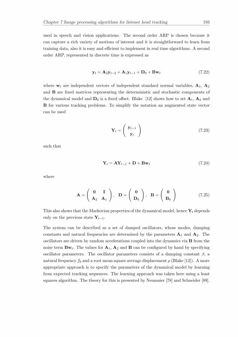
Chapter 7 Image processing algorithms for listener head tracking 193
used in speech and vision applications. The second order ARP is chosen because itcan capture a rich variety of motions of interest and it is straightforward to learn fromtraining data, also it is easy and efficient to implement in real time algorithms. A secondorder ARP, represented in discrete time is expressed as
yt = A2yt−2 + A1yt−1 + D0 + Bwt (7.22)
where wt are independent vectors of independent standard normal variables, A1, A2
and B are fixed matrices representing the deterministic and stochastic components ofthe dynamical model and D0 is a fixed offset. Blake [12] shows how to set A1, A2 andB for various tracking problems. To simplify the notation an augmented state vectorcan be used
Yt =
(yt−1
yt
)(7.23)
such that
Yt = AYt−1 + D + Bwt (7.24)
where
A =
(0 I
A2 A1
), D =
(0
D0
), B =
(0
B0
)(7.25)
This also shows that the Markovian properties of the dynamical model, hence Yt dependsonly on the previous state Yt−1.
The system can be described as a set of damped oscillators, whose modes, dampingconstants and natural frequencies are determined by the parameters A1 and A2. Theoscillators are driven by random accelerations coupled into the dynamics via B from thenoise term Bwt. The values for A1, A2 and B can be configured by hand by specifyingoscillator parameters. The oscillator parameters consists of a damping constant β, anatural frequency f0 and a root mean square average displacement ρ (Blake [12]). A moreappropriate approach is to specify the parameters of the dynamical model by learningfrom expected tracking sequences. The learning approach was taken here using a leastsquares algorithm. The theory for this is presented by Neumaier [78] and Schneider [89].
Chapter 7 Image processing algorithms for listener head tracking 194
7.4.5 Particle filters
Particle filters have been used in many fields of applied science. The use of particlefilters are due to their generality and ease of implementation, which make them suitablefor many signal processing problems. They have previously been used in for simulationsin fluid mechanics, statistical mechanics, econometrics, signal processing and computervision, in order to mention a few (MacCormick [62]). Several closely related algorithmsare known under the names sequential Monte Carlo methods, bootstrap filters, con-densation, Monte Carlo filters, interacting particle approximations and survival of thefittest [25]. The particle filter that has been applied in this thesis is the condensationalgorithm (Blake [12], Isard [41], MacCormick [62]). It has been chosen due to its suit-ability in computer vision applications and its reputation for being able to track objectsin considerable clutter.
The condensation algorithm can be used to track known objects in a video sequencewhere the background in the video sequence is not assumed to be rigid or stationaryand its three dimensional structure is unknown. It is particularly useful in cases wherethere is a significant amount of clutter in the background. Clutter is defined as elementsin the background that may be similar to parts of foreground features. The probabilitydensity for Yt = Y1, ...Yt is multi-modal, hence not even approximately Gaussian,therefore the widely used Kalman filter (based on Gaussian distributions) is not suitablefor this task.
The condensation algorithm is suitable in this more general situation and also it is inmany cases a considerably simpler algorithm than the Kalman filter. The use of randomsampling is often considered as computationally inefficient, despite the fact that thecondensation algorithm runs in near real-time. This can be achieved by using relativelytight distributions for shape, which is achieved by using accurate learned models of shapeand motion. The theory of the condensation algorithm is briefly explained in AppendixC.
7.4.6 Results
In this section, the contour tracker using the condensation algorithm is tested on clut-tered and uncluttered image sequences. The contour tracking algorithm is made totrack a single target using a single camera. The “shape space” for tracking is builtfrom a hand drawn template of the head, which is allowed to deform via planar affinetransformations (and six DOF). The initial template Q0 can be extracted from the firstframe in the video sequence. The control points are positioned around the edge of thehead and spline interpolation is performed between the control points. The initialisationof the contour tracker is a crucial matter because it will affect the performance of thewhole tracking sequence. The initialisation of the position of the contour in the im-
Chapter 7 Image processing algorithms for listener head tracking 195
age is performed with the image segmentation technique described in Section 7.2. TheARP motion model parameters are set by learning dynamics from expected trackingsequences.
7.4.6.1 Contour tracking with a plain background
The ability to track a moving persons head is tested using a video sequence of 300frames. Figure 7.16 and Figure 7.17 illustrate the tracking sequence. Representing thestate density with N = 70 samples at each time step proves sufficient for successfultracking. The contour tracker correctly estimates the head position throughout thevideo sequence. The algorithm is implemented in Matlab [66] and runs at a couple ofHz on a Pentium 4 computer. The initialisation of the spline template is performed byusing the same initialisation that the skin colour tracking algorithm uses in Section 7.2.
Figure 7.16 illustrates a number of frames from a video sequence with a plain background.The subject is mainly moving in the lateral plane. As the subject is moving around thecontour tracker follows the centre of the head closely and the shape of the head is alsoretained relatively well. Figure 7.17 illustrates a number of frames from a video sequencewith a plain background and occlusion. The subject is holding its hand in front of thehead for a couple of seconds and then moving his hand in away from the head in order todistract the contour tracker. The hand movement distracts the tracker but the trackerrecovers and the contour is fitted to head again when the hand is removed.
7.4.6.2 Contour tracking with a cluttered background
Figure 7.18 illustrates frames from a video sequence with a cluttered background. Again,the subject is mainly moving in the lateral plane and as the subject is moving aroundthe contour tracker follows the centre of the head closely. The shape of the head is alsohere retained relatively well. Figure 7.19 illustrates frames from a video sequence witha plain background and occlusion. The subject is moving his hand in front of the head(as for the plain background case) in order to distract the contour tracker. The handmovement distracts the tracker but the tracker does not lose its target and the shape ofthe contour fits the head closely after the hand is removed.
7.5 Discussion
The motivation for using a camera system for listener head tracking is the relatively lowcost of implementation and that the listener does not need to wear any sensors. Thepresented colour tracking is relatively robust to background noise, tracks the positionof the head accurately enough in terms of translation and is computationally efficient.
Chapter 7 Image processing algorithms for listener head tracking 196
One problem with the algorithm is light sensitivity, and to improve this parameter itis recommended that Nearly Infra Red (NIR) and Infra Red (IR) tracking is investi-gated. The combination of RGB bands with three narrow NIR bands is suggested byStorring [93] to robustly detect skin under changing illumination and to distinguish itfrom objects similar to skin colour. The disadvantage with this approach is the needfor a dedicated sensor instead of a standard RGB camera and the added computationalcomplexity of using six dimensions instead of three dimensions. Another shortcoming isthat for some applications it is desirable to include listener rotation, which the colourtracking algorithm can not handle. The colour tracking algorithm can be suitable forapplications where the listener is facing in a certain known direction, such as when ascreen is present. The colour tracking algorithm can be extended to robust tracking ofmultiple listeners.
The stereo area correlation process for finding the distance to the listener can possiblybe replaced by using “blob” size as a measure for distance. Since, the size of the colourblob that represents the head is proportional to the distance between the camera andthe head. However, the accuracy of the distance measure is likely to be significantly lessthan for the stereo area correlation algorithm. A drawback with using stereo tracking isobviously the need for two cameras.
The contour algorithm is recommended if the listener is allowed to move more freelyand when there is plenty of clutter in the environment. The contour algorithm is morerobust with respect to background noise compared to the colour tracking algorithm.The contour tracking algorithm can also be extended to robust tracking of multiplelisteners (MacCormick [62]) as well as to track listener rotation. The particle filter thatwas incorporated in contour tracking framework adds predictive capabilities that canpossibly reduce filter update times. The main disadvantage of the contour trackingalgorithm is the computational effort it requires.
An interesting algorithm that has not been evaluated in this thesis is eye tracking. Thepossibility of using eyes as a feature to track is interesting especially for systems witha screen, such as a TV or desktop computer. Eye tracking can also be used to verifythat the listener is still present in the view field of the camera and can be applied forexample in the ROI of the colour tracking algorithm.
Another promising application for image processing in virtual sound imaging is pinnashape detection. Image processing can be used to detect the shape of the listeners pinna,which then can be mapped to an approximately individual HRTF [56].
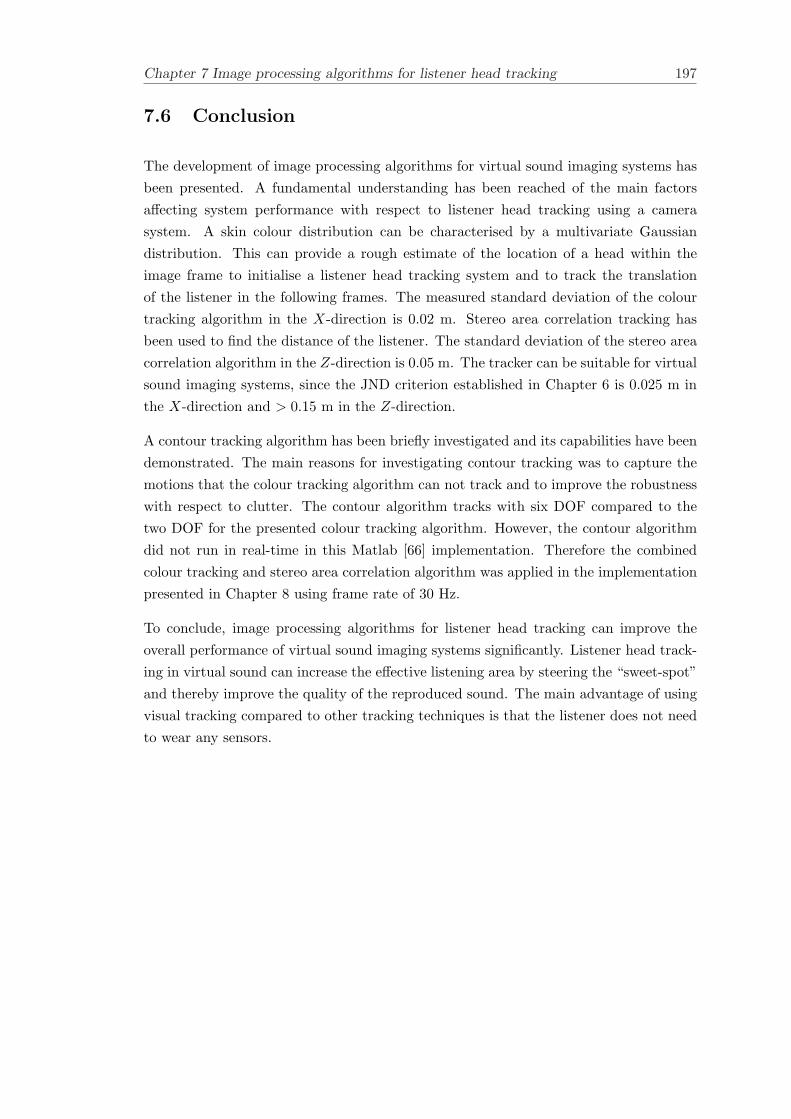
Chapter 7 Image processing algorithms for listener head tracking 197
7.6 Conclusion
The development of image processing algorithms for virtual sound imaging systems hasbeen presented. A fundamental understanding has been reached of the main factorsaffecting system performance with respect to listener head tracking using a camerasystem. A skin colour distribution can be characterised by a multivariate Gaussiandistribution. This can provide a rough estimate of the location of a head within theimage frame to initialise a listener head tracking system and to track the translationof the listener in the following frames. The measured standard deviation of the colourtracking algorithm in the X-direction is 0.02 m. Stereo area correlation tracking hasbeen used to find the distance of the listener. The standard deviation of the stereo areacorrelation algorithm in the Z-direction is 0.05 m. The tracker can be suitable for virtualsound imaging systems, since the JND criterion established in Chapter 6 is 0.025 m inthe X-direction and > 0.15 m in the Z-direction.
A contour tracking algorithm has been briefly investigated and its capabilities have beendemonstrated. The main reasons for investigating contour tracking was to capture themotions that the colour tracking algorithm can not track and to improve the robustnesswith respect to clutter. The contour algorithm tracks with six DOF compared to thetwo DOF for the presented colour tracking algorithm. However, the contour algorithmdid not run in real-time in this Matlab [66] implementation. Therefore the combinedcolour tracking and stereo area correlation algorithm was applied in the implementationpresented in Chapter 8 using frame rate of 30 Hz.
To conclude, image processing algorithms for listener head tracking can improve theoverall performance of virtual sound imaging systems significantly. Listener head track-ing in virtual sound can increase the effective listening area by steering the “sweet-spot”and thereby improve the quality of the reproduced sound. The main advantage of usingvisual tracking compared to other tracking techniques is that the listener does not needto wear any sensors.
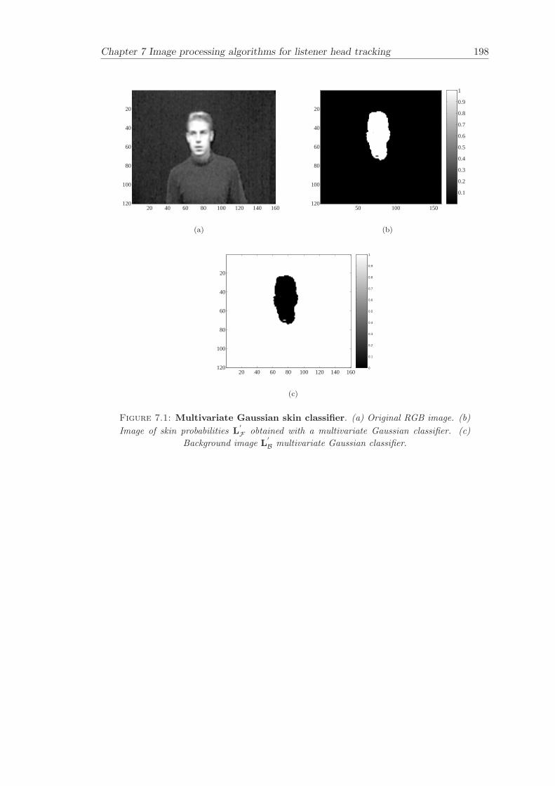
Chapter 7 Image processing algorithms for listener head tracking 198
20 40 60 80 100 120 140 160
20
40
60
80
100
120
(a)
50 100 150
20
40
60
80
100
120
0.1
0.2
0.3
0.4
0.5
0.6
0.7
0.8
0.9
1
(b)
20 40 60 80 100 120 140 160
20
40
60
80
100
120 0
0.1
0.2
0.3
0.4
0.5
0.6
0.7
0.8
0.9
1
(c)
Figure 7.1: Multivariate Gaussian skin classifier. (a) Original RGB image. (b)Image of skin probabilities L
′F obtained with a multivariate Gaussian classifier. (c)
Background image L′B multivariate Gaussian classifier.
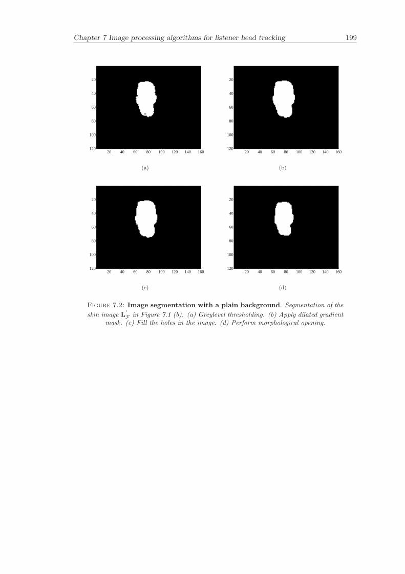
Chapter 7 Image processing algorithms for listener head tracking 199
20 40 60 80 100 120 140 160
20
40
60
80
100
120
(a)
20 40 60 80 100 120 140 160
20
40
60
80
100
120
(b)
20 40 60 80 100 120 140 160
20
40
60
80
100
120
(c)
20 40 60 80 100 120 140 160
20
40
60
80
100
120
(d)
Figure 7.2: Image segmentation with a plain background. Segmentation of theskin image L
′F in Figure 7.1 (b). (a) Greylevel thresholding. (b) Apply dilated gradient
mask. (c) Fill the holes in the image. (d) Perform morphological opening.
Chapter 7 Image processing algorithms for listener head tracking 200
20 40 60 80 100 120 140 160
20
40
60
80
100
120
(a)
50 100 150
20
40
60
80
100
120 0
0.1
0.2
0.3
0.4
0.5
0.6
0.7
0.8
0.9
(b)
20 40 60 80 100 120 140 160
20
40
60
80
100
120
(c)
20 40 60 80 100 120 140 160
20
40
60
80
100
120
(d)
20 40 60 80 100 120 140 160
20
40
60
80
100
120
(e)
20 40 60 80 100 120 140 160
20
40
60
80
100
120
(f)
Figure 7.3: Image segmentation with clutter. Segmentation of skin image L′F
where the objects hand is present. (a) Original RGB image. (b) Image of skin probabil-ities L
′F obtained with a multivariate normal classifier. (c) Greylevel thresholding. (d)
Apply dilated gradient mask. (e) Fill the holes in the image. (f) Perform morphologicalopening.
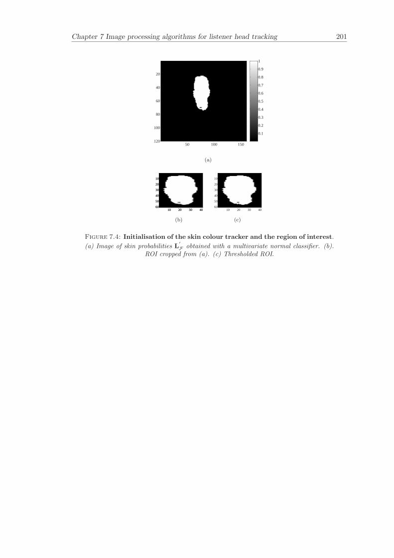
Chapter 7 Image processing algorithms for listener head tracking 201
50 100 150
20
40
60
80
100
120
0.1
0.2
0.3
0.4
0.5
0.6
0.7
0.8
0.9
1
(a)
10 20 30 40
10
20
30
40
50
6010 20 30 40
10
20
30
40
50
60
(b)
10 20 30 40
10
20
30
40
50
60
(c)
Figure 7.4: Initialisation of the skin colour tracker and the region of interest.(a) Image of skin probabilities L
′F obtained with a multivariate normal classifier. (b).
ROI cropped from (a). (c) Thresholded ROI.
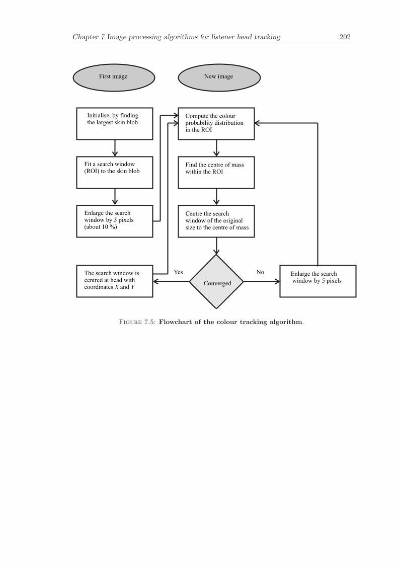
Chapter 7 Image processing algorithms for listener head tracking 202
Initialise, by findingthe largest skin blob
Fit a search window(ROI) to the skin blob
Enlarge the searchwindow by 5 pixels(about 10 %)
Compute the colourprobability distributionin the ROI
Find the centre of masswithin the ROI
Centre the searchwindow of the originalsize to the centre of mass
Enlarge the searchwindow by 5 pixels
First image New image
Converged
NoYesThe search window iscentred at head withcoordinates andX Y
Figure 7.5: Flowchart of the colour tracking algorithm.
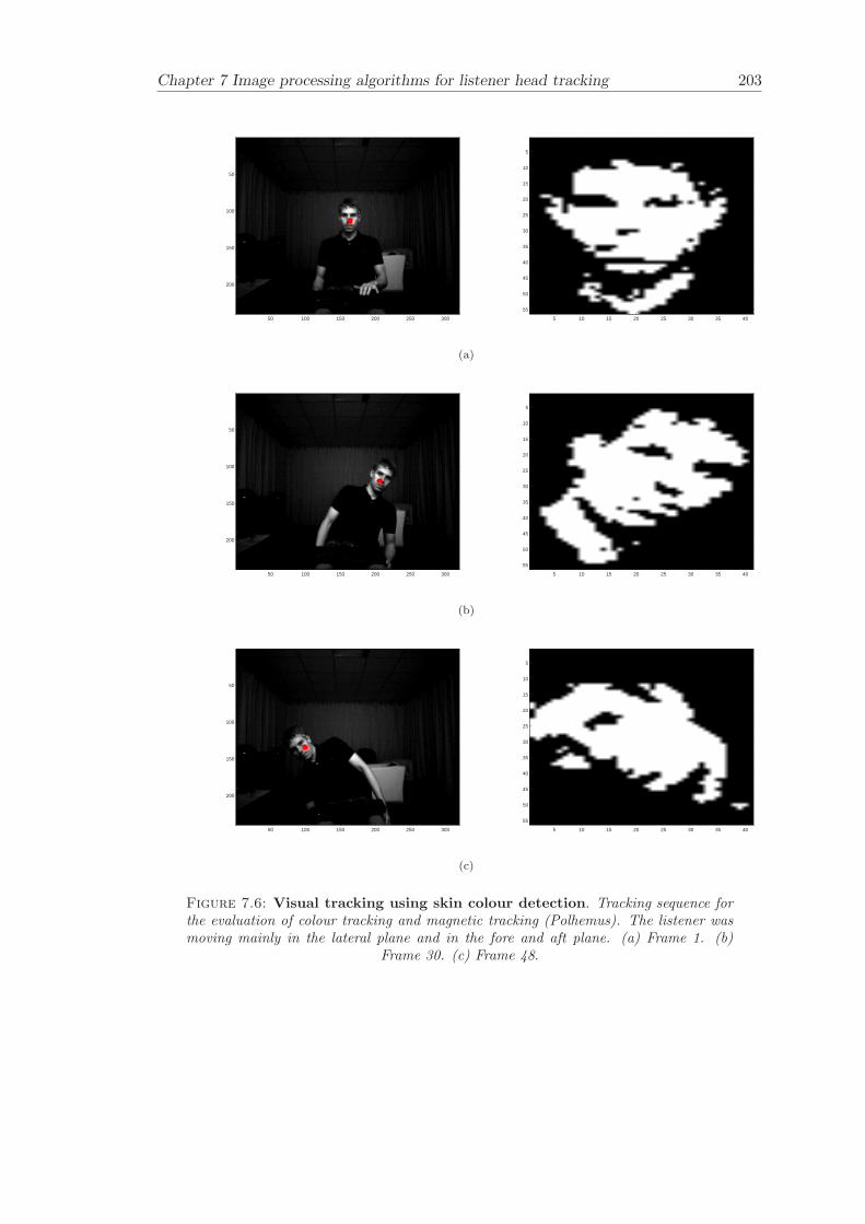
Chapter 7 Image processing algorithms for listener head tracking 203
50 100 150 200 250 300
50
100
150
200
5 10 15 20 25 30 35 40
5
10
15
20
25
30
35
40
45
50
55
(a)
50 100 150 200 250 300
50
100
150
200
5 10 15 20 25 30 35 40
5
10
15
20
25
30
35
40
45
50
55
(b)
50 100 150 200 250 300
50
100
150
200
5 10 15 20 25 30 35 40
5
10
15
20
25
30
35
40
45
50
55
(c)
Figure 7.6: Visual tracking using skin colour detection. Tracking sequence forthe evaluation of colour tracking and magnetic tracking (Polhemus). The listener wasmoving mainly in the lateral plane and in the fore and aft plane. (a) Frame 1. (b)
Frame 30. (c) Frame 48.
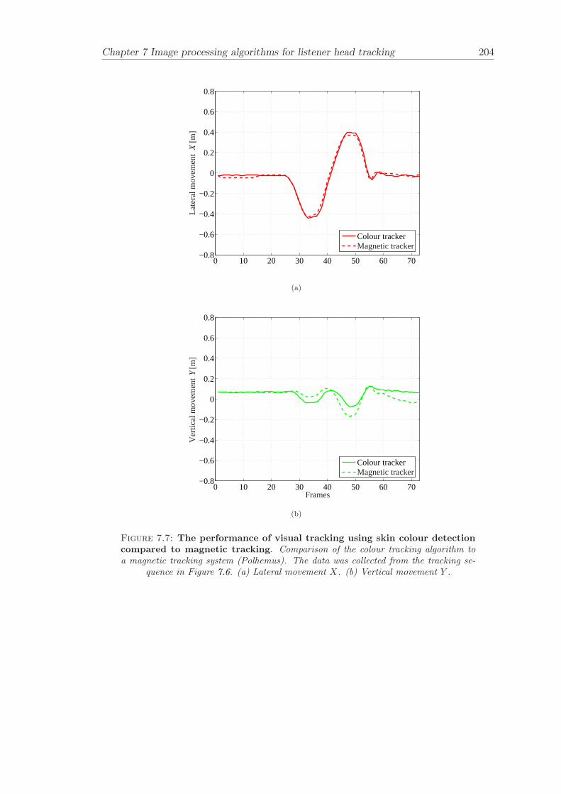
Chapter 7 Image processing algorithms for listener head tracking 204
0 10 20 30 40 50 60 70−0.8
−0.6
−0.4
−0.2
0
0.2
0.4
0.6
0.8
Late
ral m
ovem
ent X
[m]
Colour trackerMagnetic tracker
(a)
0 10 20 30 40 50 60 70−0.8
−0.6
−0.4
−0.2
0
0.2
0.4
0.6
0.8
Ver
tical
mov
emen
t Y [m
]
Frames
Colour trackerMagnetic tracker
(b)
Figure 7.7: The performance of visual tracking using skin colour detectioncompared to magnetic tracking. Comparison of the colour tracking algorithm toa magnetic tracking system (Polhemus). The data was collected from the tracking se-
quence in Figure 7.6. (a) Lateral movement X. (b) Vertical movement Y .
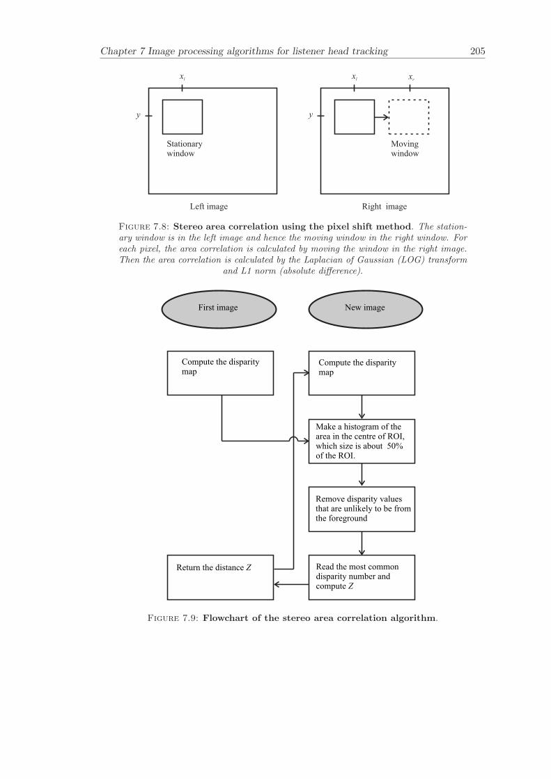
Chapter 7 Image processing algorithms for listener head tracking 205
Stationarywindow
Movingwindow
Left image Right image
y y
xlxl xr
Figure 7.8: Stereo area correlation using the pixel shift method. The station-ary window is in the left image and hence the moving window in the right window. Foreach pixel, the area correlation is calculated by moving the window in the right image.Then the area correlation is calculated by the Laplacian of Gaussian (LOG) transform
and L1 norm (absolute difference).
Compute the disparitymap
Compute the disparitymap
Make a histogram of thearea in the centre of ROI,which size is about 50%of the ROI.
Remove disparity valuesthat are unlikely to be fromthe foreground
Read the most commondisparity number andcompute Z
First image New image
Return the distance Z
Figure 7.9: Flowchart of the stereo area correlation algorithm.
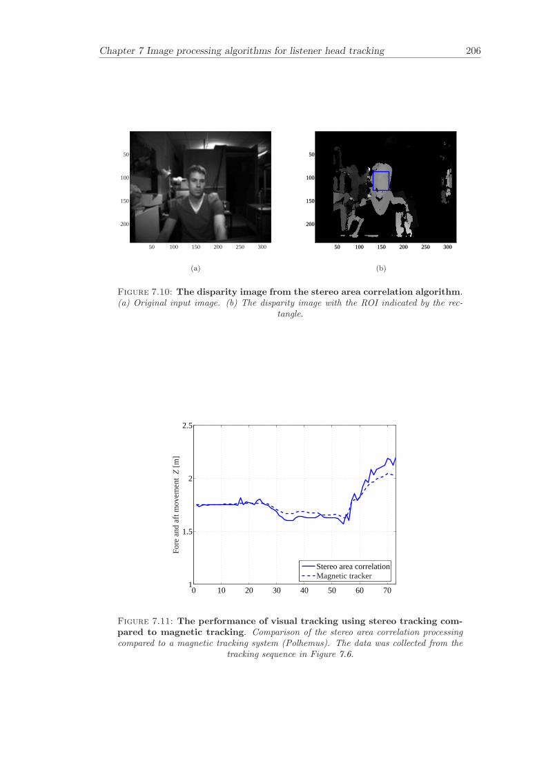
Chapter 7 Image processing algorithms for listener head tracking 206
50 100 150 200 250 300
50
100
150
200
(a)
50 100 150 200 250 300
50
100
150
200
50 100 150 200 250 300
50
100
150
200
(b)
Figure 7.10: The disparity image from the stereo area correlation algorithm.(a) Original input image. (b) The disparity image with the ROI indicated by the rec-
tangle.
0 10 20 30 40 50 60 701
1.5
2
2.5
Fore
and
aft
mov
emen
t Z
[m
]
Stereo area correlationMagnetic tracker
Figure 7.11: The performance of visual tracking using stereo tracking com-pared to magnetic tracking. Comparison of the stereo area correlation processingcompared to a magnetic tracking system (Polhemus). The data was collected from the
tracking sequence in Figure 7.6.
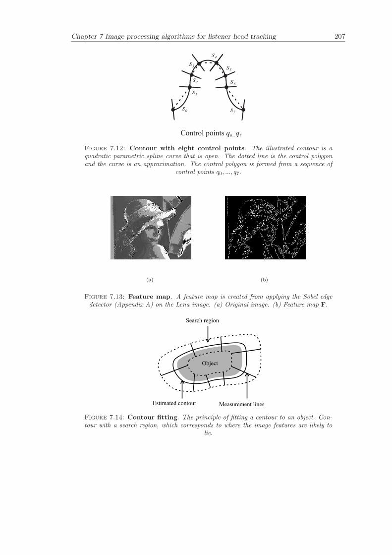
Chapter 7 Image processing algorithms for listener head tracking 207
s0
s1
s2
s3
s4
s5
s6
s7
Control points q q0... 7
Figure 7.12: Contour with eight control points. The illustrated contour is aquadratic parametric spline curve that is open. The dotted line is the control polygonand the curve is an approximation. The control polygon is formed from a sequence of
control points q0, ..., q7.
(a) (b)
Figure 7.13: Feature map. A feature map is created from applying the Sobel edgedetector (Appendix A) on the Lena image. (a) Original image. (b) Feature map F.
Object
Measurement linesEstimated contour
Search region
Figure 7.14: Contour fitting. The principle of fitting a contour to an object. Con-tour with a search region, which corresponds to where the image features are likely to
lie.
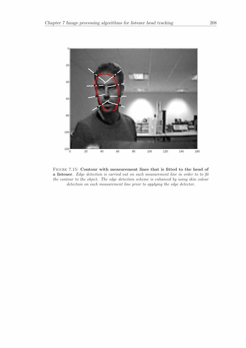
Chapter 7 Image processing algorithms for listener head tracking 208
0 20 40 60 80 100 120 140 160
0
20
40
60
80
100
120
Figure 7.15: Contour with measurement lines that is fitted to the head ofa listener. Edge detection is carried out on each measurement line in order to to fitthe contour to the object. The edge detection scheme is enhanced by using skin colour
detection on each measurement line prior to applying the edge detector.
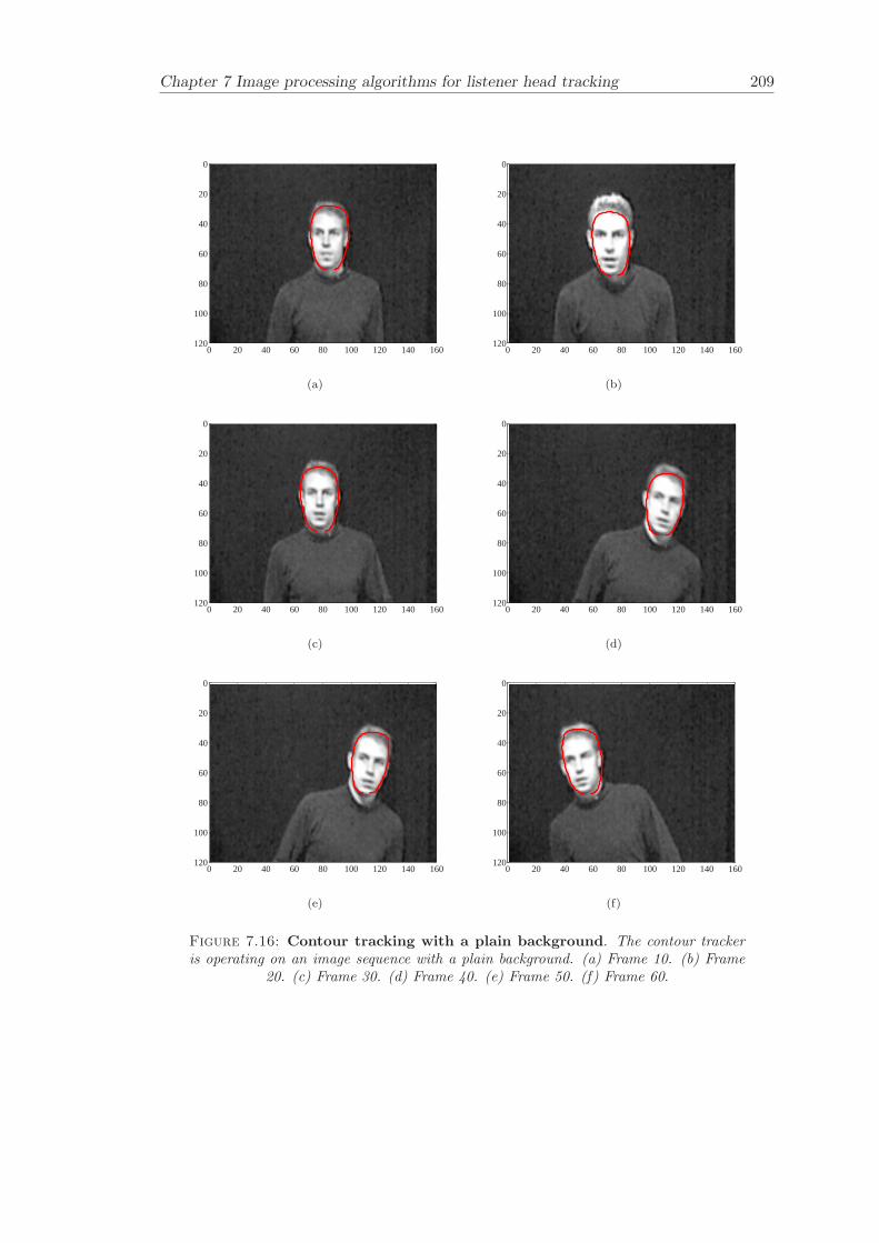
Chapter 7 Image processing algorithms for listener head tracking 209
0 20 40 60 80 100 120 140 160
0
20
40
60
80
100
120
(a)
0 20 40 60 80 100 120 140 160
0
20
40
60
80
100
120
(b)
0 20 40 60 80 100 120 140 160
0
20
40
60
80
100
120
(c)
0 20 40 60 80 100 120 140 160
0
20
40
60
80
100
120
(d)
0 20 40 60 80 100 120 140 160
0
20
40
60
80
100
120
(e)
0 20 40 60 80 100 120 140 160
0
20
40
60
80
100
120
(f)
Figure 7.16: Contour tracking with a plain background. The contour trackeris operating on an image sequence with a plain background. (a) Frame 10. (b) Frame
20. (c) Frame 30. (d) Frame 40. (e) Frame 50. (f) Frame 60.
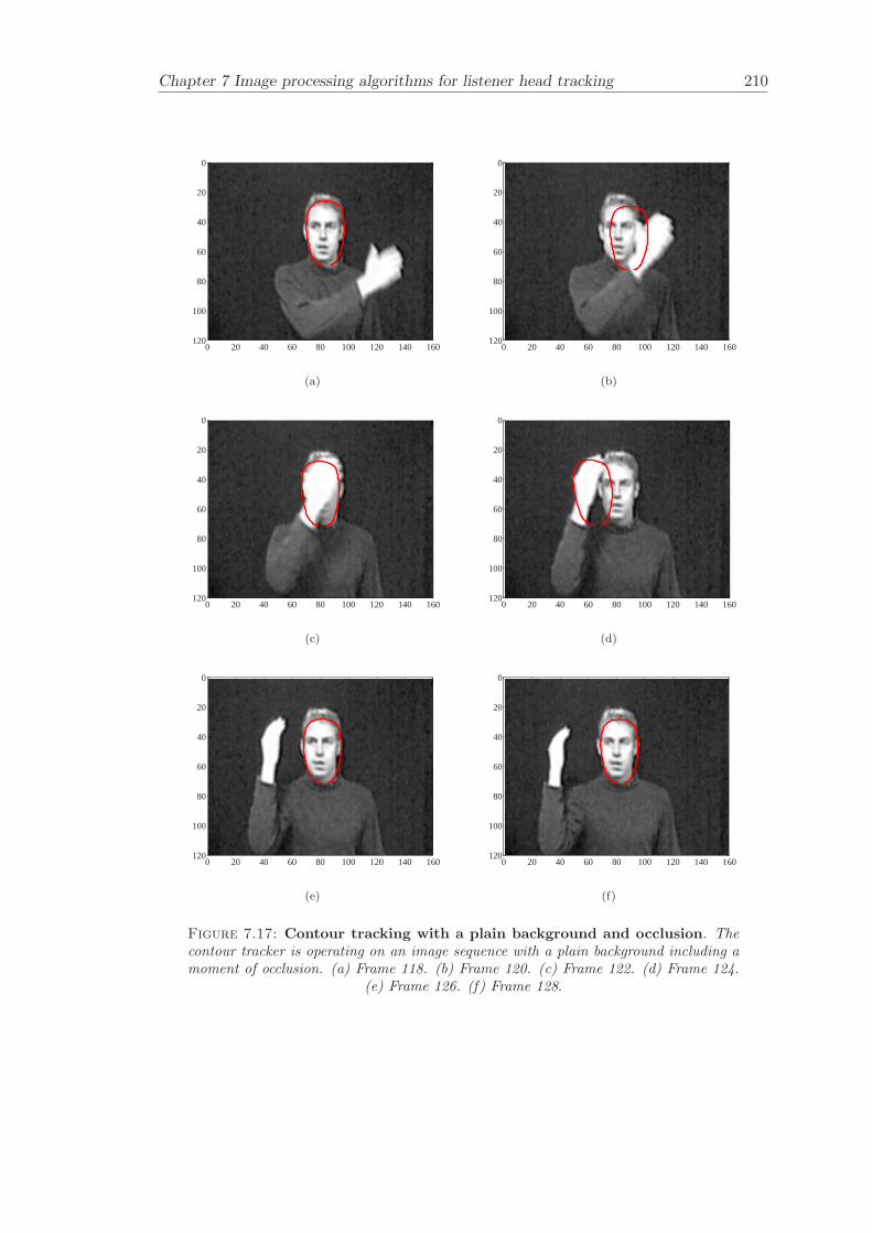
Chapter 7 Image processing algorithms for listener head tracking 210
0 20 40 60 80 100 120 140 160
0
20
40
60
80
100
120
(a)
0 20 40 60 80 100 120 140 160
0
20
40
60
80
100
120
(b)
0 20 40 60 80 100 120 140 160
0
20
40
60
80
100
120
(c)
0 20 40 60 80 100 120 140 160
0
20
40
60
80
100
120
(d)
0 20 40 60 80 100 120 140 160
0
20
40
60
80
100
120
(e)
0 20 40 60 80 100 120 140 160
0
20
40
60
80
100
120
(f)
Figure 7.17: Contour tracking with a plain background and occlusion. Thecontour tracker is operating on an image sequence with a plain background including amoment of occlusion. (a) Frame 118. (b) Frame 120. (c) Frame 122. (d) Frame 124.
(e) Frame 126. (f) Frame 128.
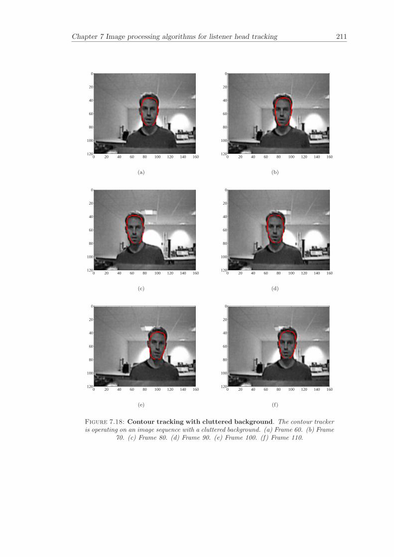
Chapter 7 Image processing algorithms for listener head tracking 211
0 20 40 60 80 100 120 140 160
0
20
40
60
80
100
120
(a)
0 20 40 60 80 100 120 140 160
0
20
40
60
80
100
120
(b)
0 20 40 60 80 100 120 140 160
0
20
40
60
80
100
120
(c)
0 20 40 60 80 100 120 140 160
0
20
40
60
80
100
120
(d)
0 20 40 60 80 100 120 140 160
0
20
40
60
80
100
120
(e)
0 20 40 60 80 100 120 140 160
0
20
40
60
80
100
120
(f)
Figure 7.18: Contour tracking with cluttered background. The contour trackeris operating on an image sequence with a cluttered background. (a) Frame 60. (b) Frame
70. (c) Frame 80. (d) Frame 90. (e) Frame 100. (f) Frame 110.
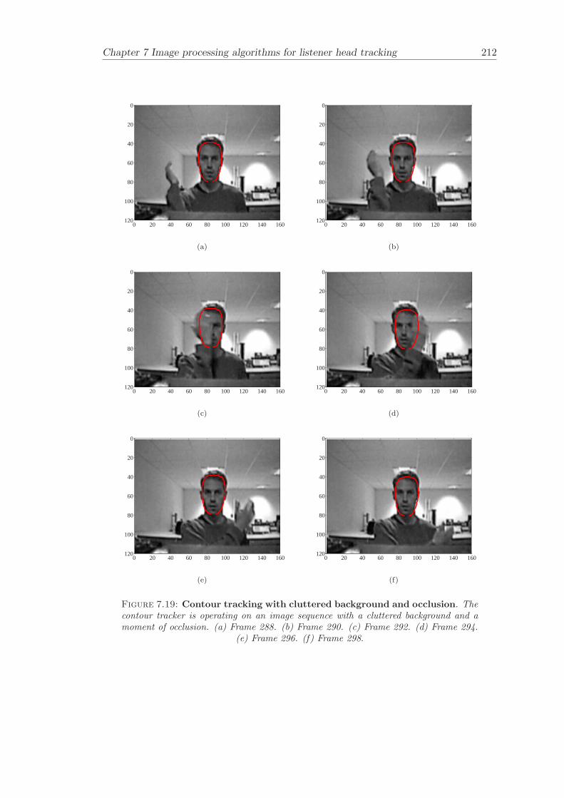
Chapter 7 Image processing algorithms for listener head tracking 212
0 20 40 60 80 100 120 140 160
0
20
40
60
80
100
120
(a)
0 20 40 60 80 100 120 140 160
0
20
40
60
80
100
120
(b)
0 20 40 60 80 100 120 140 160
0
20
40
60
80
100
120
(c)
0 20 40 60 80 100 120 140 160
0
20
40
60
80
100
120
(d)
0 20 40 60 80 100 120 140 160
0
20
40
60
80
100
120
(e)
0 20 40 60 80 100 120 140 160
0
20
40
60
80
100
120
(f)
Figure 7.19: Contour tracking with cluttered background and occlusion. Thecontour tracker is operating on an image sequence with a cluttered background and amoment of occlusion. (a) Frame 288. (b) Frame 290. (c) Frame 292. (d) Frame 294.
(e) Frame 296. (f) Frame 298.
Chapter 8
Experiments on an integrated
system
The implementation of a visually adaptive SD system is introduced that combines visualhead tracking and binaural sound reproduction. The system is capable of tracking theposition of the listener in the lateral plane and in the fore and aft plane while dynami-cally updating the cross-talk cancellation filters. The algorithms are implemented usinga software approach on a Pentium 4 computer. The realized filter update algorithmis described in detail. The performance of cross-talk cancellation filters and the filterupdate algorithm is objectively evaluated through measurements in an anechoic cham-ber. The results from the objective evaluation are compared to previously presentedsubjective experiments.
3D sound for virtual reality and multimedia applications is presented by Begault [11]and to quote him “it is impossible to predict the position of the listener or of the speak-ers in any given situation”, although this is true for any given situation, under certainconstraints it is possible to track the position of the listener relative to the loudspeakers.Here it has been shown that it is possible to track the position of a listener that is notwearing any sensors using image processing techniques. The constraints on the imple-mented algorithm require that the background has to have a different colour distributioncompared to the face of listener and the light during tracking has to be consistent withthe light when the listener skin sample was chosen.
A realisation of an adaptive cross-talk cancellation system for a moving listener is pre-sented by Lentz [59]. The system is based on static cross-talk cancellation that is updateddepending on the listener’s position. Listening tests show that the dynamic cross-talkcancellation produces impressive results and that the listener can move in an area ofabout 1 m2. This system uses a magnetic head tracking system with a sensor attachedto the listener. More recently Lentz [60], [58] has developed the adaptive cross-talk can-cellation system further to include four loudspeakers, which can support 360 listener
213
Chapter 8 Experiments on an integrated system 214
rotation. The system includes room-specific simulation, dynamic cross-talk cancellationand multi-track binaural synthesis. The head tracking is performed with a commer-cial infrared tracking system that requires the user to wear markers that the infraredcameras can detect. The system is configured in a CAVE like environment, which is afive sided projection system of a rectangular shape installed at RWTH Aachen Univer-sity. An other example of virtual sound imaging system is the DIVA project [88], whichwas designed in order to produce a real-time environment for immersive audiovisualprocessing.
8.1 System
The visually adaptive system that was developed at the ISVR, University of Southamp-ton is described here. The system is implemented in a first version and it is open toany extended virtual sound modelling applications in real-time. The system is namedVSI (Virtual Sound Imaging) and developed using object oriented programming (C++).The aim was to write a program that could be used on a standard computer. The cur-rent version is optimised for a Pentium 4 computer and runs on a single processor.In order to run both the image processing and the audio signal processing on a singleprocessor requires highly efficient algorithms. Therefore, the image processing algorithmthat was implemented needed to be relatively simple in order to keep the computationalcost to a minimum. The currently implemented colour tracking fulfils the efficiencyrequirements. The most demanding parts of the audio signal processing comprise of thefast-deconvolution algorithm and the partitioned convolution process.
There are other solutions already available for the audio signal processing like the LakeHuron system. Though, the Huron is a highly specialised system that is also limited interms of the real time filter switching capabilities that was required for the VSI system.The VSI system is different from previous approaches from several viewpoints. Thesystem adapts the sweet spot position dynamically for a moving listener without the needfor the user to wear any sensors. The system is not limited to any constrained hardwarerequirements, such as specific audio DSP technology. The audio signal processing part ofthe system is realised using a software approach and can be used with readily availablecomputer hardware.
The system layout is illustrated by the diagram in Figure 8.1. The head tracking al-gorithm finds the listener position and passes the value to the thresholding part of thesystem. The threshold for lateral movement corresponds to a 1 change in azimuth angleand the threshold for fore and aft movement is configured to 0.03 m. The fore and aftcoordinates are smoothed by a moving average filter using 10 averages. This introducessome un-wanted lag. However, the precision of the estimate of the fore and aft coor-dinate does not need to be as precise as for the lateral coordinate, and the introduced
Chapter 8 Experiments on an integrated system 215
lag can be accepted if the listener mainly moves in the lateral plane. New inverse filtersare computed when the threshold for listener movement is breached. The filters arecomputed by choosing the closest HRTF pairs from an ITD-equalised database with aresolution of 1. The delay information in the measured HRTF database is removed inadvance by the interpolation algorithm described in Section 4.1. The database that wasused here holds 512 coefficients including the on-axis loudspeaker response. The delayand amplitude scaling models for the filter calculation are based on the far field sphericalradiation approximation. A Hanning window of the same length as the inverse filter isapplied in order to avoid ringing effects. The inverse filters are then updated as describedby the partitioned convolution and commutation process described in Section 8.2. Thesound output device is configured with the Audio Stream Input Output (ASIO) proto-col, which was designed for professional audio recording. The ASIO protocol providesan interface between an application and the sound card.
8.2 Partitioned convolution and commutation
Binaural sound reproduction using loudspeakers requires multichannel convolution andfor adaptive systems it is also desirable to have a low latency between the filter updates.Partitioned convolution provides low input/output delay in the convolution process. Foran adaptive loudspeaker system it is necessary to update the inverse filters accordingto where the listener is positioned. The filter update process results in audible artifactsif the inverse filters are updated on too coarse a grid. Therefore commutation canbe used in order to remove the audible artifacts. This section shows the theory forpartitioned convolution and how a commutation scheme can be implemented directly inthe partitioned convolution algorithm in order to make it suitable for adaptive cross-talkcancellation.
The cross-talk cancellation scheme is performed by convolving the two input signals withfour inverse filters. These inverse filters are computed by chosing appropriate HRTFsand using the fast-deconvolution algorithm. The convolution task can be simplified byperforming FFTs and IFFTs, since time domain convolution becomes multiplicationin the frequency domain. The FFT assumes inherently that the analysed segment isperiodic, which leads to unsatisfactory results if a straightforward block by block imple-mentation in the frequency domain is used. Therefore, the periodicity of the FFTs needsto be removed from the output sequence. This can be achieved by using the overlap andsave algorithm, which is illustrated in Figure 8.2. The input window of M samples isshifted to the right over the input sequence of M −N samples, and then convolution isperformed for the following segment. The disadvantage is that FFTs of lengths M > N
are necessary. A common configuration for the overlap-and-save algorithm is to haveM = 2×N , which also gives the best efficiency (Torger [98]).
Chapter 8 Experiments on an integrated system 216
The partitioned overlap-and-save algorithm is the one that has been used in this project.It was first proposed by Stockham [92] and further developed for real-time implemen-tation by Soo [91]. Torger [98] has previously used partitioned convolution for binauralsound reproduction. Firstly, the impulse response of the inverse filter st(n) is partitionedinto a suitable number of P blocks of equal size, which is illustrated in Figure 8.3. Theneach partition is convolved by a standard overlap-and-save process with FFTs of lengthsL (here L = 2 × K). In the process, zero padding is used for making each block L
samples in length, and the transformation into the frequency domain is carried out withthe FFT, which results in a number of frequency domain filters Πi,t(k). These frequencydomain filters Πi,t(k) are multiplied by the FFTs of the input blocks and then IFFTsare used to revert to the time domain and the result is summed as described in Figure8.4. This process gives the same result as the un-partitioned convolution, but with themain difference that the latency of the partitioned convolution process is only L samplescompared to M samples. Hence, the input/output delay can be controlled by choosinga suitable value for L.
The commutation process is implemented directly in the partitioned convolution algo-rithm. The relationship between old, new and commutated coefficients are as follows
Πi,c(k) =(
Nc − i
Nc
)Πi,a(k) +
i
NcΠi,b(k) (8.1)
where the commutated inverse filter block is labeled Πi,c(k), the previous inverse filterΠi,a(k) and the new inverse filter Πi,b(k). The commutated inverse filter Πi,c(k) is thenupdated for each new block Π1,c(k), Π2,c(k) . . . ,ΠNc,c(k). For example, if the filter issegmented into 8 blocks and there are 16 commutation steps, then each of the inversefilter coefficients are switched in 2 steps, as illustrated in Figure 8.5.
The commutation process is carried out in real-time by dynamically updating the co-efficients. The commutation technique described here uses FIR filtering and an ITD-equalised non-minimum phase HRTF database. The non-minimum phase characteristiccan result in comb filtering effects in the frequency domain due to phase differences be-tween the interpolated HRTFs. The non-minimum phase FIR approximation has beenfound to produce severe comb filtering effects if the phase delays vary considerably. Thismay occur if the resolution of the HRTF database is > 10 − 15 (Huopaniemi [38]).However, this can be minimized by using a fine resolution in the HRTF database, likethe 1 resolution used here.
8.3 Filter update rate
The time it takes between the update of a new listener position and for the outputsignal to be generated with the newly calculated filters is the latency of the system.
Chapter 8 Experiments on an integrated system 217
The output buffer of the sound card and the block length of the partitioned convolutionalgorithm is 256 coefficients. This results in a latency of 5.8 ms at a sampling rate of44.1 kHz for the output of a single block. The fast-deconvolution algorithm takes 6 msto compute a new set of inverse filters (2048 coefficients) in the current configuration(Pentium 4 computer). A filter length of 2048 coefficients at a sampling frequency of 44.1kHz correspond to 45.2 ms in the time domain. The image processing algorithm takes 10ms to compute a new position for the current implementation of the colour tracking andstereo area correlation algorithms. However, the image processing algorithm updatesthe images at a frame rate of 30 Hz, which is the upper limit of the current hardwareconfiguration, which leads to a delay of 33.3 ms for finding the new listener position.If the commutation and partitioned convolution algorithm is configured to 8 partitionsand 8 steps of commutation, the resulting time it takes for a complete new inverse filterto be present on the output is 45.2 + 5.8 + 33.3 + 6 = 90.3 ms. If the commutationpart is left out and the filters are updated directly, then the latency for the new filterto become active would be 5.8 + 33.3 + 6 = 45.1 ms. This could be further reduced ifthe camera system would run at higher frame rate of for example 60 Hz, which wouldresult in a latency of 5.8 + 16.7 + 6 = 28.5 ms.
The update rate of the real-time system is an important aspect here. The filter updaterate has been studied intensively by subjective experiments. Two criteria for filterupdates namely the JND and JNC criteria were established in Chapter 6. In order toapply these criteria it is important to know the velocity of the movements of the listener.A field study by Lentz [60] shows that the mean translational velocity is at 0.15 m/s fortheir CAVE configuration. The CAVE allows the listener to walk around in an area of acouple of m2. The listener position in the VSI system is updated for lateral movementwhen the angle of an HRTF has changed by 1. This results in a filter update every0.035 m at a distance of 2 m away from the loudspeakers. If the listener moves at 0.15m/s in the lateral plane then a filter update occurs every 233 ms. If listener rotation isallowed, then less delay would be required for the filter update, according to field studiesby Lentz [60], a recalculation of the inverse filters needs to be carried out every 10-20ms with a filter update rate of 35 ms.
The filter update algorithm that was implemented is close to matching the JND cri-teria at 2 m distance for the listener. The filter updates in the lateral plane every 1
of change in HRTF angle. This corresponds to 0.035 m at 2 m distance on-axis. TheJND criterion in the lateral plane is slightly higher and was found to be approximately0.025 m in Chapter 6. However, the filter update criteria was established using bandlim-ited white noise as a stimulus and preliminary listening tests suggests that when usingmusic and speech signals the update rate can be coarser to some extent. The systemconfiguration with 8 partitions and 24 commutation steps also fulfills the JNC criterion.The filter coefficients are on average stepped 0.012 m in this configuration (8 parti-tions, 24 commutation steps), which is close to the JNC criterion that was determined
Chapter 8 Experiments on an integrated system 218
to be approximately 0.012 m. Hence, the filter update algorithm can be configuredwith 8 partitions and 24 commutation steps as a default in order to comply with datafrom subjective experiments. The time it takes for a complete filter update using thisconfiguration is (3× 45.2) + 5.8 + 33.3 + 6 = 180.7 ms.
The filter update rate can be reduced by using shorter inverse filters. The inverse filterlength of 2048 coefficients used here can possibly be reduced by cropping out the 1024most important coefficients and still keeping the delay intact (Lentz [60]). It could bereduced further by using a database of HRTFs that contains less coefficients. An alter-native filter update technique could possibly be used. The outputs from two adjacentinverse filters could be “cross-faded” instead of the commutation process described inSection 8.2. The result from this has not been investigated here. However, it would taketwice as many inverse filters in the convolution process, i.e. 8 filters instead of 4 filters.This leads to a more computationally demanding algorithm but with the advantage ofpossibly reducing the filter update rate. The cross-fading technique can also be usedwith IIR filters, which can reduce the number of filter coefficients and the computa-tional effort. Another method for reducing the time lag in the system is to use a listenertracking algorithm that predicts the future listener position, such as the “condensation”algorithm (Blake [12]).
8.4 Evaluation of filter updates
An objective evaluation of the implemented filter update algorithm was undertaken. Theaim was to determine how well the filter update algorithm would perform for differentconfigurations with respect to the number of partitions and commutation steps. Threedifferent configurations using different numbers of partitions and commutation stepswere evaluated.
The system was configured in an anechoic chamber at the ISVR as is illustrated inFigure 8.6. The SD loudspeaker configuration was used and the KEMAR dummy headwas used for measuring the filter updates. The distance between the loudspeakers andthe KEMAR was 2 m and the source signal was a 1 kHz sine wave. The loudspeakerswere moved in front of the KEMAR and the visually adaptive system was configured totrack the dummy head. The loudspeakers were moving at a rate of 0.01 m/s, which wasthe maximum allowed rate of change for the loudspeaker moving rig that was available.The loudspeakers were moved from on-axis to 0.2 m to the right of the dummy headin the lateral plane. The source signal used in this experiment was a 1 kHz sine wavethat was played from the VSI system and then recorded with the KEMAR dummy headconnected to the Huron measurement system. The database in the software was thesmall pinna with open ear canal and with the on-axis loudspeaker response included.The same loudspeakers that were used for the HRTF database measurement were used
Chapter 8 Experiments on an integrated system 219
here so that the loudspeaker response could be included. The KEMAR had the sameconfiguration as when the HRTF database was measured, i.e. configured with the smallpinna and the open ear canal.
In order to evaluate the filter update scheme, a different number of partitions and com-mutation steps were investigated for a filter length of 2048 samples. The first configu-ration holds 2 partitions and 2 steps of commutation, the aim was to simulate a directfilter update (the software could not be configured for un-partitioned convolution with-out rewriting the code). The second configuration uses 8 partitions and 8 steps in thecommutation scheme. This aims to show how the software can perform in a configura-tion with a block size of 256 samples using a minimum amount of commutation. Thethird configuration uses 8 partitions and 48 steps of commutation. The number of com-mutation steps are increased to show the smoothness that can be achieved in a filtertransition.
The results are presented in the time domain in Figure 8.7 for a 1 kHz source signal(reference). Figure 8.7 (a) illustrates the case when the loudspeaker is fixed at on-axisand 1 kHz source signal is played during 20 s. It can be seen that the configurationwith 2 partitions and 2 commutation steps results in unwanted spikes during the filterupdate. The configuration with 8 partitions and 8 commutation steps illustrates thatthe spikes are removed but the filter updates seems to be quite sharp still. The lastconfiguration with 8 partitions and 48 commutation steps illustrates that the spikes areremoved and that a much more smooth transition is achieved.
The same measurement data as in Figure 8.7 are here presented in a time-frequency plotin Figure 8.8. The spectra is here represented by the magnitude of the short-time Fouriertransform as described in Oppenheim [80]. The time-frequency plots were created usingthe following parameters: a block size of 2048 samples, a frequency discretisation of4096 samples and an overlap of 1536 samples. These values where chosen to enhancethe clarity of the filter updates. The extra components in the reference spectra shown inFigure 8.8 (a) are due to harmonics produced by the loudspeakers and the amplifier. InFigure 8.8 (b)-(d) there are additional components created by the step motor that wasunfortunately quite noisy. The vertical lines in the spectra are due to the filter updates.The results in Figure 8.8 (b) clearly indicates high frequency noise that is audible byhuman hearing. Figure 8.8 (c) illustrates that the filter update is not as pronounced asin the previous case when increasing the number of commutation steps. Figure 8.8 (d)illustrates that the an increasing number of commutation step results in a significantlysmoother filter transition.
Chapter 8 Experiments on an integrated system 220
8.5 Evaluation of the effectiveness of cross-talk cancella-
tion
The cross-talk cancellation performance was measured in an anechoic chamber using thesame system configuration as in the filter update evaluation above. The measurementwas carried out in the lateral plane from -35 cm to 35 cm relative to on-axis in 5 cmsteps. The measurement was carried out using the Huron workstation. The sourcesignal was bandlimited white noise (300-20000 Hz) of 32768 samples long and 10 timesaveraging was applied in the evaluation of spectra. The source signal was loaded intothe software and played from there. The KEMAR was connected to the Huron in orderto record the resulting signals. The measurement data was further averaged 20 timesduring post-processing.
The measured system cross-talk cancellation performance is illustrated for the staticsystem in Figure 8.9 and for the adaptive system in Figure 8.10. Figure 8.9 (a) illustratesthe signal P11(k) (as defined in Equation 2.29). It can be observed that there are bothpeaks and dips present in the frequency response as the listener moves off-axis. Figure8.9 (b) illustrates the signal P21(k). The cross-talk cancellation performance is in theregion of 15 dB on-axis and degrades to around 0 dB with additional peaks and dipsdepending on listener position. The sweet-spot appears to be in the region of a coupleof cm depending on frequency and channel separation.
Figure 8.10 (a) illustrates the signal P11(k) and it can be observed that the frequencyresponse is similar for all lateral positions with some difference mainly at frequenciesabove 7000 Hz. Figure 8.10 (b) illustrates the signal P21(k) and it can be seen thatthe cross-talk cancellation performance is in the region of 15 dB for all measured lateralpositions up to approximately 7000 Hz, where the pinna resonance occurs.
8.6 Conclusion
An evaluation of a visually adaptive virtual sound imaging system has been presented.The system is capable of reproducing binaural signals at the ears of a moving listenerthat is not wearing any sensors. The listener is allowed to move in the lateral planeand in the fore and aft plane. The system is implemented using a software approachand readily available computer equipment. The software that has been designed can beextended to include any desired virtual sound application. An innovative filter updatealgorithm has been introduced that can be implemented directly in the partitionedconvolution process. The performance of the filter update algorithm has been evaluatedby measurements in an anechoic chamber. The results shows that the filter updatealgorithm manages to produce smooth filter updates in its current application. Theresults from the filter update evaluation have been compared to previous subjective

Chapter 8 Experiments on an integrated system 221
experiments. It has been illustrated how the filter update algorithm can be configuredto comply with the subjective filter update criteria, JND and JNC that were establishedin Chapter 6. The cross-talk cancellation performance for static and adaptive systemshas been evaluated under anechoic conditions. The features of the measurement datashows similarities to those in the simulations presented in Section 5.3.
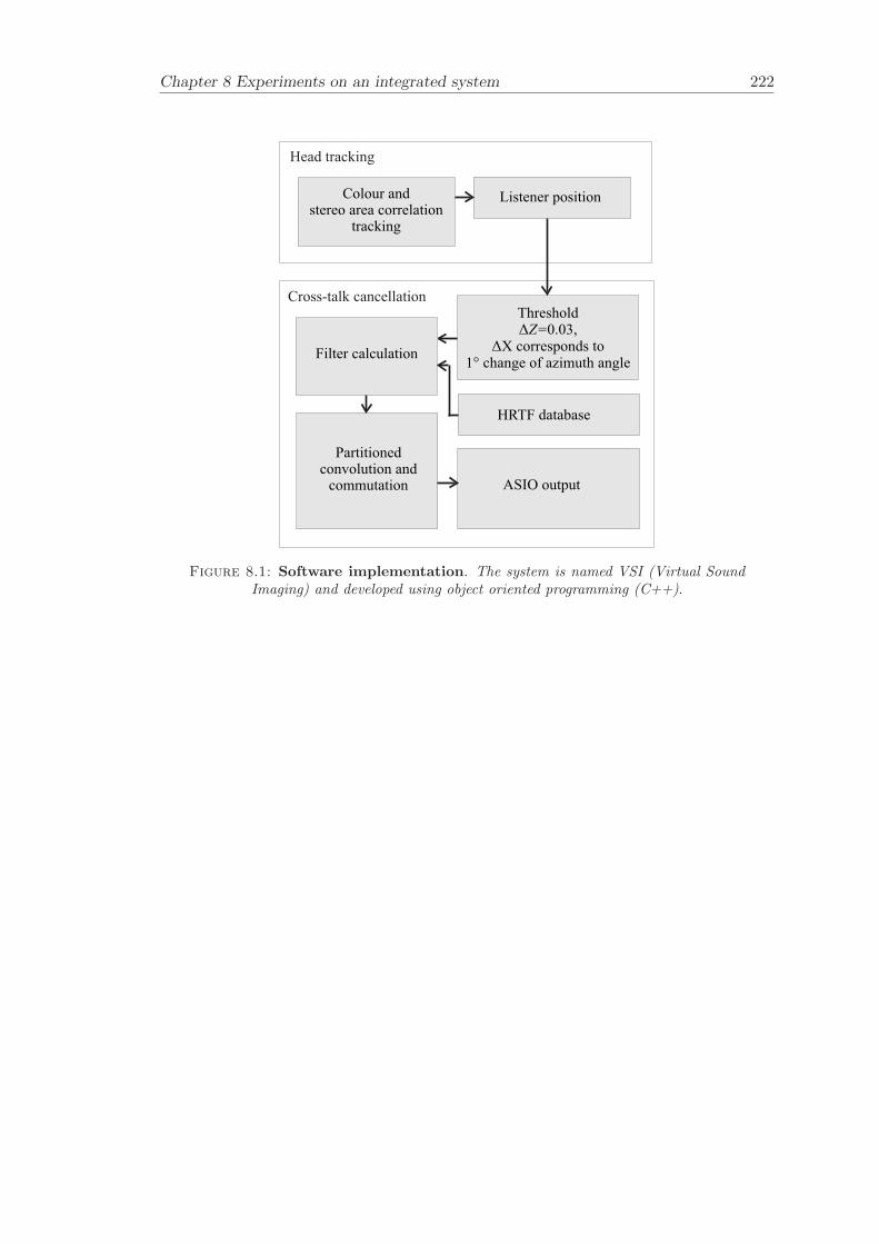
Chapter 8 Experiments on an integrated system 222
Head tracking
Cross-talk cancellation
Listener position
Threshold0.03,
X corresponds to1 change of azimuth angle
Z=ΔΔ
°
HRTF database
Filter calculation
Partitionedconvolution and
commutation ASIO output
Colour andstereo area correlation
tracking
Figure 8.1: Software implementation. The system is named VSI (Virtual SoundImaging) and developed using object oriented programming (C++).
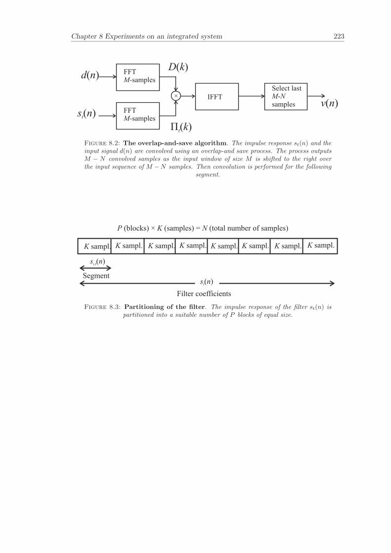
Chapter 8 Experiments on an integrated system 223
FFT-samplesM
FFT-samplesM
IFFT
Select last-
samplesM N×
d n( )
v n( )
Πt( )k
D k( )
s nt( )
Figure 8.2: The overlap-and-save algorithm. The impulse response st(n) and theinput signal d(n) are convolved using an overlap-and save process. The process outputsM − N convolved samples as the input window of size M is shifted to the right overthe input sequence of M −N samples. Then convolution is performed for the following
segment.
K sampl. K sampl. K sampl. K sampl. K sampl. K sampl. K sampl. K sampl.
P K N(blocks) (samples) = (total number of samples)×
s nt( )
s ni,t( )
Segment
Filter coefficients
Figure 8.3: Partitioning of the filter. The impulse response of the filter st(n) ispartitioned into a suitable number of P blocks of equal size.
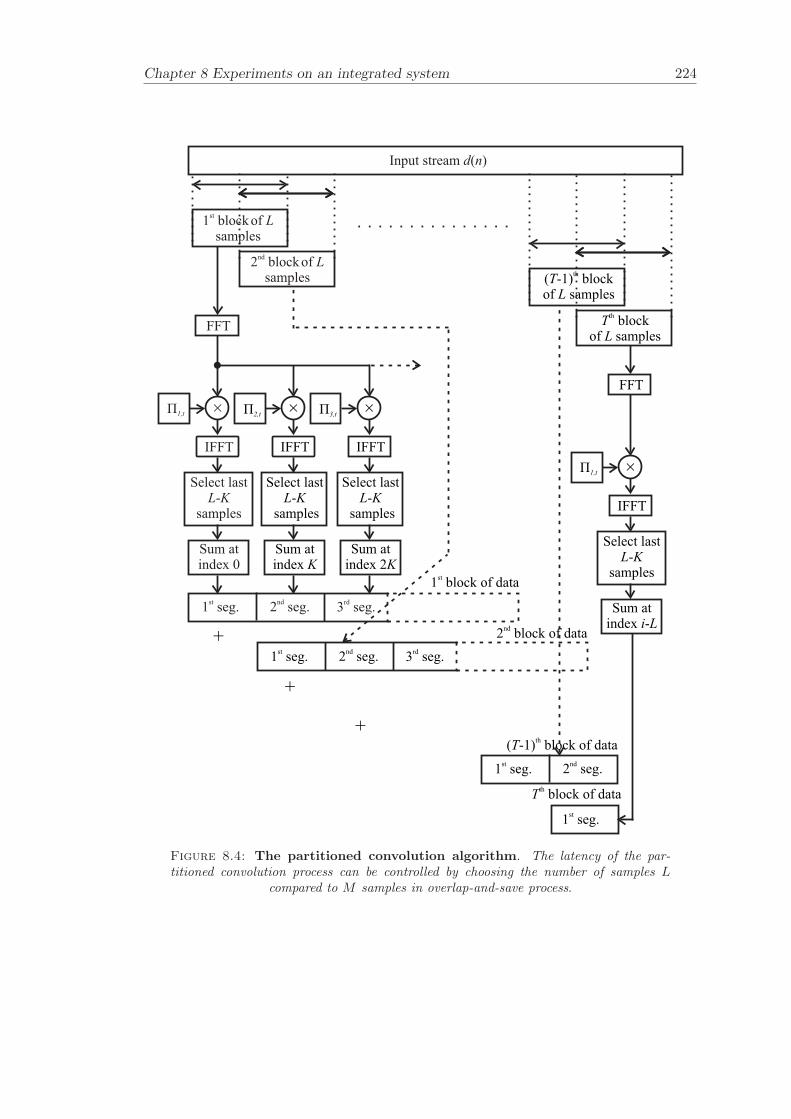
Chapter 8 Experiments on an integrated system 224
Input stream ( )d n
1 blockofsamples
stL
2 blockofsamples
ndL
FFT
×Π1,t
Select last-
samplesL K
IFFT
Sum atindex 0
1 seg.st
2 seg.nd
3 seg.rd
1 block of datast
1 seg.st
2 seg.nd
3 seg.rd
2 block of datand
+
+
+( -1) block of dataT
th
1 seg.st
2 seg.nd
1 seg.st
Tth
block of data
×Π2,t
Select last-
samplesL K
IFFT
Sum atindex K
×Π3,t
Select last-
samplesL K
IFFT
Sum atindex 2K
FFT
×Π1,t
Select last-
samplesL K
IFFT
Sum atindex -i L
( -1) blockof samplesT
L
th
T
L
thblock
of samples
Figure 8.4: The partitioned convolution algorithm. The latency of the par-titioned convolution process can be controlled by choosing the number of samples L
compared to M samples in overlap-and-save process.

Chapter 8 Experiments on an integrated system 225
Π1,cΠ2,c Π3,c Π4,c Π5,c Π6,c Π7,c Π8,c
Π9,c Π10,c Π11,c Π12,c Π13,c Π14 Π15,c Π16,c
1 filter of × cross-faded coefficientsst
K P
2 of ×nd
K Pfilter cross-faded coefficients
,c
Figure 8.5: The commutation step in the partitioned convolution algorithm.In this example, the filter is partitioned into 8 blocks and switched in 16 steps.
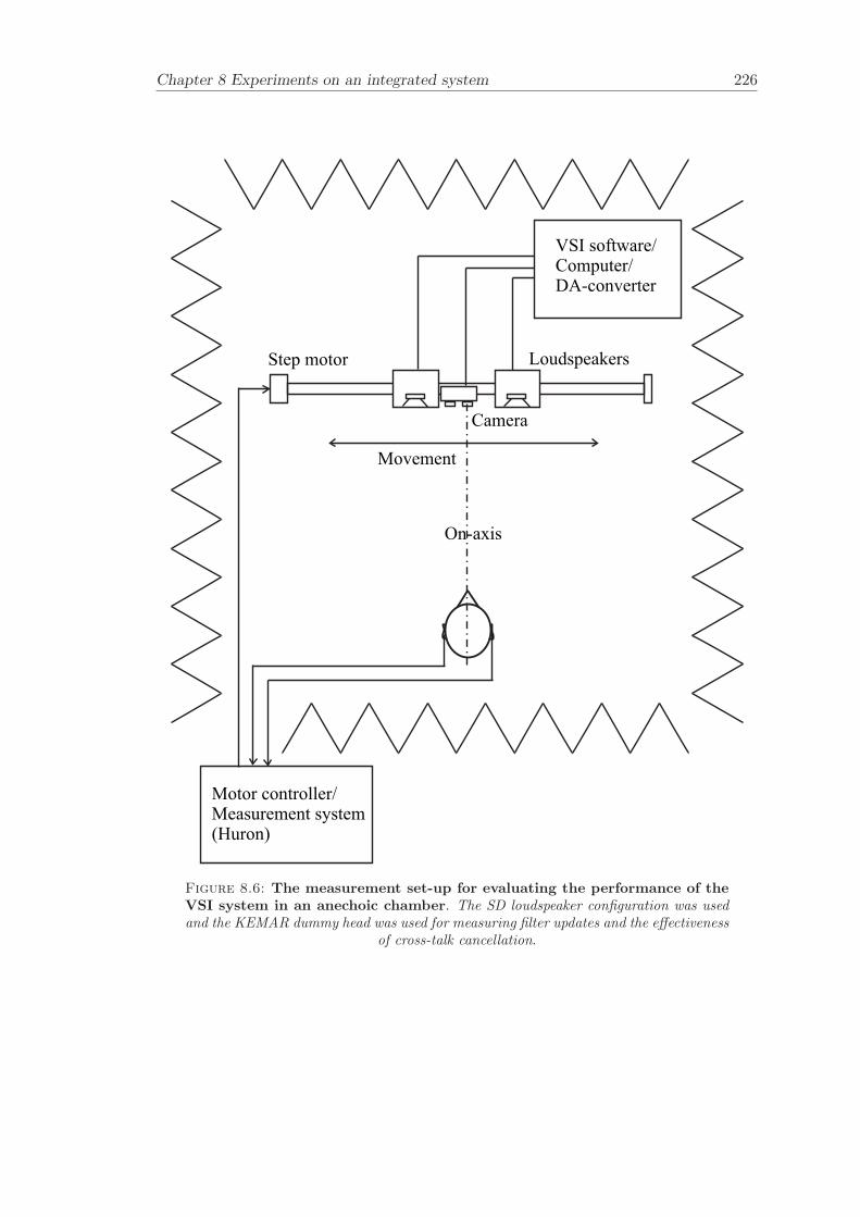
Chapter 8 Experiments on an integrated system 226
Motor controller/Measurement system(Huron)
VSI software/
DA-converterComputer/
Movement
Step motor Loudspeakers
Camera
On-axis
Figure 8.6: The measurement set-up for evaluating the performance of theVSI system in an anechoic chamber. The SD loudspeaker configuration was usedand the KEMAR dummy head was used for measuring filter updates and the effectiveness
of cross-talk cancellation.
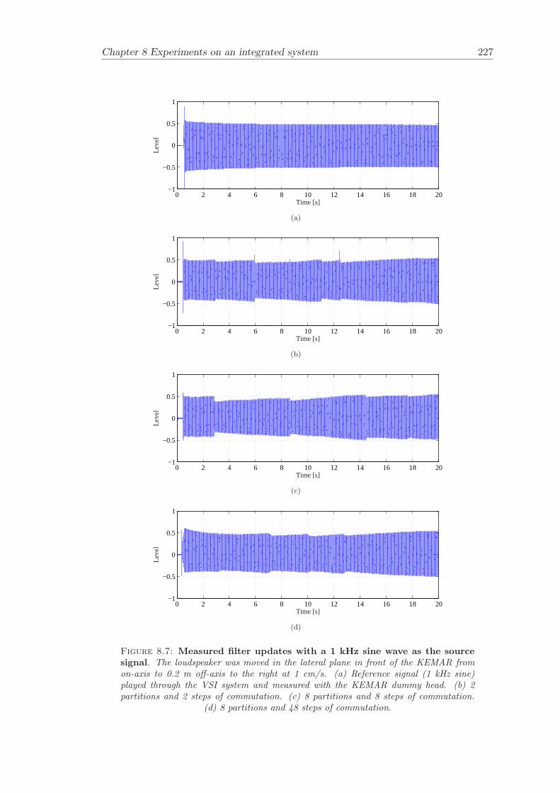
Chapter 8 Experiments on an integrated system 227
0 2 4 6 8 10 12 14 16 18 20−1
−0.5
0
0.5
1
Time [s]
Leve
l
(a)
0 2 4 6 8 10 12 14 16 18 20−1
−0.5
0
0.5
1
Time [s]
Leve
l
(b)
0 2 4 6 8 10 12 14 16 18 20−1
−0.5
0
0.5
1
Time [s]
Leve
l
(c)
0 2 4 6 8 10 12 14 16 18 20−1
−0.5
0
0.5
1
Time [s]
Leve
l
(d)
Figure 8.7: Measured filter updates with a 1 kHz sine wave as the sourcesignal. The loudspeaker was moved in the lateral plane in front of the KEMAR fromon-axis to 0.2 m off-axis to the right at 1 cm/s. (a) Reference signal (1 kHz sine)played through the VSI system and measured with the KEMAR dummy head. (b) 2partitions and 2 steps of commutation. (c) 8 partitions and 8 steps of commutation.
(d) 8 partitions and 48 steps of commutation.
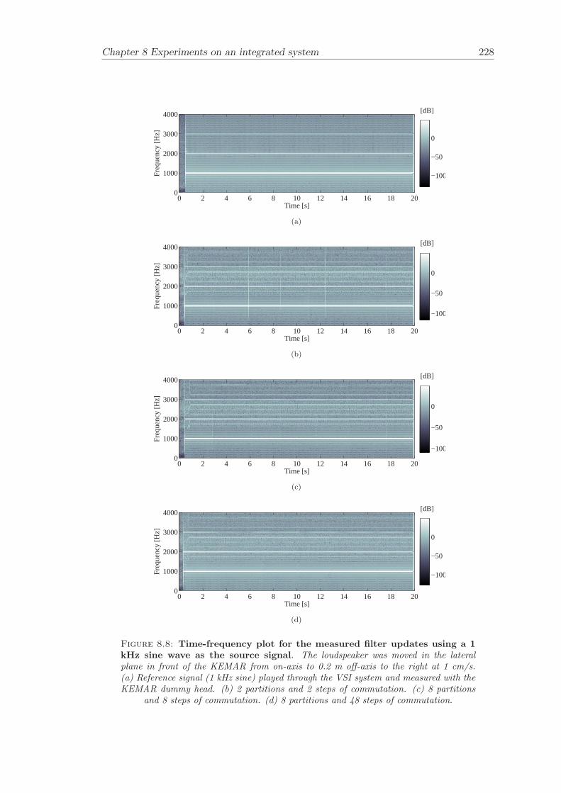
Chapter 8 Experiments on an integrated system 228
[dB]
Time [s]
Fre
quen
cy [H
z]
0 2 4 6 8 10 12 14 16 18 200
1000
2000
3000
4000
−100
−50
0
(a)
[dB]
Time [s]
Fre
quen
cy [H
z]
0 2 4 6 8 10 12 14 16 18 200
1000
2000
3000
4000
−100
−50
0
(b)
[dB]
Time [s]
Fre
quen
cy [H
z]
0 2 4 6 8 10 12 14 16 18 200
1000
2000
3000
4000
−100
−50
0
(c)
[dB]
Time [s]
Fre
quen
cy [H
z]
0 2 4 6 8 10 12 14 16 18 200
1000
2000
3000
4000
−100
−50
0
(d)
Figure 8.8: Time-frequency plot for the measured filter updates using a 1kHz sine wave as the source signal. The loudspeaker was moved in the lateralplane in front of the KEMAR from on-axis to 0.2 m off-axis to the right at 1 cm/s.(a) Reference signal (1 kHz sine) played through the VSI system and measured with theKEMAR dummy head. (b) 2 partitions and 2 steps of commutation. (c) 8 partitions
and 8 steps of commutation. (d) 8 partitions and 48 steps of commutation.
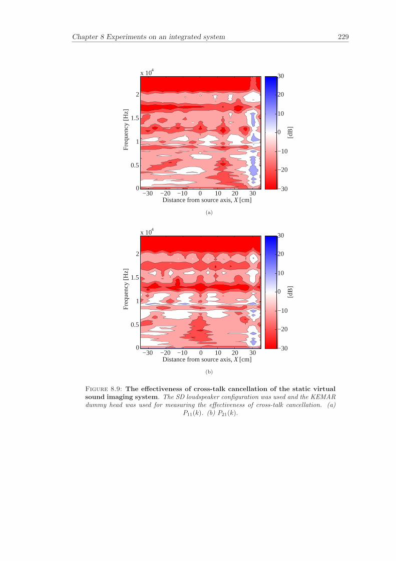
Chapter 8 Experiments on an integrated system 229
Fre
quen
cy [H
z]
Distance from source axis, X [cm]−30 −20 −10 0 10 20 30
0
0.5
1
1.5
2
x 104
[dB
]
−30
−20
−10
0
10
20
30
(a)
Fre
quen
cy [H
z]
Distance from source axis, X [cm]−30 −20 −10 0 10 20 30
0
0.5
1
1.5
2
x 104
[dB
]
−30
−20
−10
0
10
20
30
(b)
Figure 8.9: The effectiveness of cross-talk cancellation of the static virtualsound imaging system. The SD loudspeaker configuration was used and the KEMARdummy head was used for measuring the effectiveness of cross-talk cancellation. (a)
P11(k). (b) P21(k).
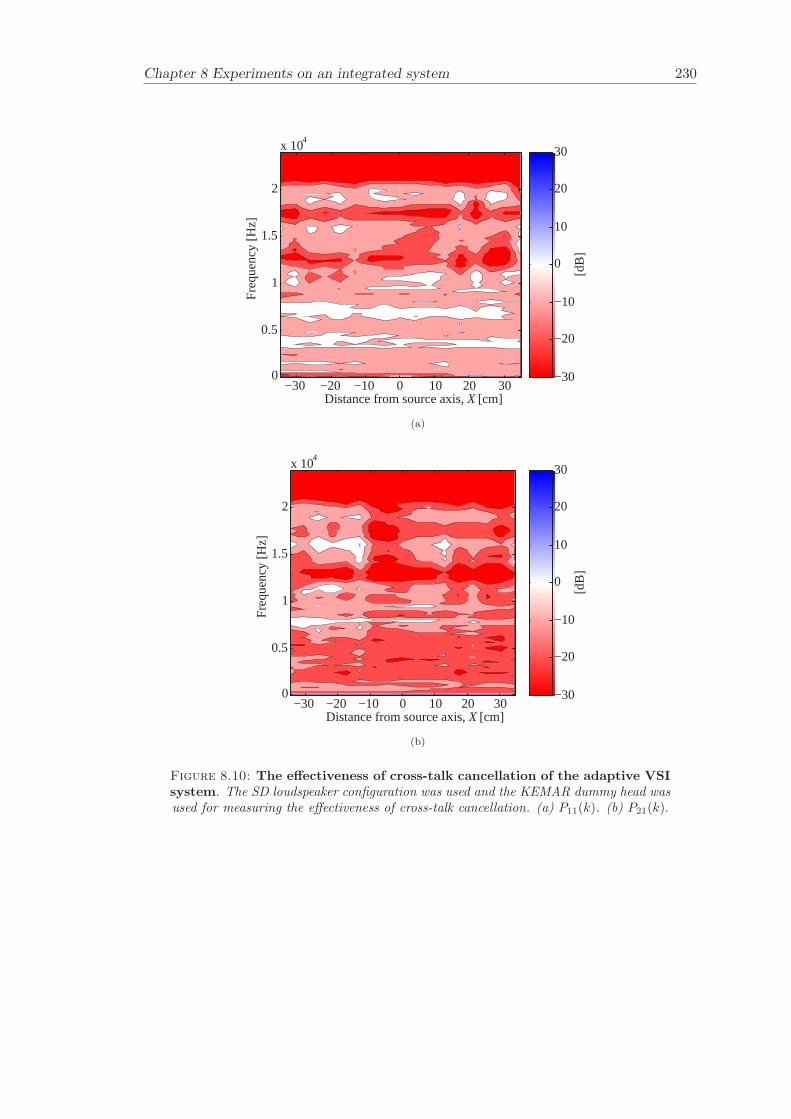
Chapter 8 Experiments on an integrated system 230
Fre
quen
cy [H
z]
Distance from source axis, X [cm]−30 −20 −10 0 10 20 30
0
0.5
1
1.5
2
x 104
[dB
]
−30
−20
−10
0
10
20
30
(a)
Fre
quen
cy [H
z]
Distance from source axis, X [cm]−30 −20 −10 0 10 20 30
0
0.5
1
1.5
2
x 104
[dB
]
−30
−20
−10
0
10
20
30
(b)
Figure 8.10: The effectiveness of cross-talk cancellation of the adaptive VSIsystem. The SD loudspeaker configuration was used and the KEMAR dummy head wasused for measuring the effectiveness of cross-talk cancellation. (a) P11(k). (b) P21(k).
Chapter 9
Conclusions
It has been demonstrated that visually adaptive virtual sound imaging systems cangenerate convincing virtual sound images under both anechoic and realistic listeningconditions. The problem addressed has been to update the inverse filters without cre-ating any audible changes for a moving listener that does not wear any sensors. Theadaptation to listener position has been carried out by using a video camera to trackhead movements and update the inverse filters accordingly. Image processing algorithmsthat successfully tracks the listener have been presented together with filter update algo-rithms and the extent of the “operational area”. The filter update algorithms have beenevaluated by subjective experiments in both an anechoic environment and in a listeningroom. The geometry of the system has been evaluated by an analytical evaluation andan objective evaluation. The results show the extent of the operational area under cer-tain performance criteria for different configurations of loudspeaker systems. Cross-overdesign techniques using a fixed and adaptive approach have been introduced since theoptimal cross-over frequencies change with the geometry of the system.
There is a strong relationship between cross-talk cancellation performance for virtualsound imaging systems and the condition number of the matrix of transfer functionsthat needs to be inverted. The dependency of condition number on frequency has beendemonstrated for asymmetric and symmetric listener positions. The “operational area”where the “sweet-spot” can be moved within can be estimated using an analytical model.The size of the operational area using a performance criterion has been shown for theStereo Dipole (SD) and the 3-way Optimal Source Distribution (OSD). The problemof designing cross-overs has been addressed where the respective advantages betweenusing fixed or adaptive cross-overs have been illustrated and recommendations havebeen made.
The measurement of a database of Head Related Transfer Functions (HRTFs) based onthe KEMAR dummy head has been carried out. The most important features of theHRTFs were illustrated. The database was measured for six different combinations of
231
Chapter 9 Conclusions 232
pinna and ear canal in order to provide extensive future modelling opportunities. Thecombination of all the six databases will enable the clear identification of the effect ofthe pinna on the HRTF. Also it is possible that “no pinna” models may be useful inthe design of virtual sound imaging systems. However, the choice of database may varybetween loudspeaker and headphone based systems.
Interpolation between Head Related Impulse Responses (HRIRs) have been investigatedand it has been found that a time domain technique named onset detection by thresh-olding performs surprisingly well. The average percentage mean square error is less than0.52% when head shadowing does not occur, in the presence of head shadowing the er-ror goes up to approximately 7.52%. The advantage of this technique is its robustnessand inherent simplicity. This interpolation algorithm has proven to be a useful tool forinverse filter design and it can also be applied in filter update algorithms.
Inverse filter design and cross-talk cancellation effectiveness for three different audiosystems has been investigated. The filter design process of cross-talk cancellation net-works using a minimum number of inverse filters has been demonstrated. The presentedfilter design technique can reduce the number of filters for Frequency Distributed Loud-speakers (FDL) to the same number as for 2-channel systems. Cross-talk cancellationeffectiveness using the fast-deconvolution algorithm has been evaluated for various fil-ter lengths and by varying the listener position/orientation. The “sweet-spot” of staticloudspeaker based binaural sound systems is very limited, which have been illustratedby simulations of the control performance under anechoic conditions. The benefit ofusing an adaptive approach where the cross-talk cancellation filters are updated to thelisteners location and orientation have been demonstrated and compared to the staticcase. The results show that the area within which the listener can move is significantlylarger in the adaptive case compared to the static case. The size of the area depends onthe degradation of performance that can be accepted compared to the optimal listeningposition and has been determined by introducing a performance criterion.
The problem of updating inverse filters in real-time have been investigated and twodifferent approaches to the solution have been presented. The filter update rates havebeen determined by defining two criteria namely, the Just Noticeable Difference (JND)criterion and the Just Noticeable (JNC) criterion. Subjective evaluations from both ananechoic chamber and a listening room show that the JND criterion is approximately0.025 m for movements in the lateral plane. The JND criterion for movements in thefore and aft plane is greater than the distance of ±0.15 m that was explored. TheJNC criterion is approximately 0.012 m for movements in the lateral plane in both theanechoic chamber and in the listening room. These results suggest that the filter updatetechniques and sound source localisation using binaural loudspeaker based systems workseffectively under anechoic as well as under non-anechoic listening conditions.
It has been demonstrated that image processing algorithms can be used to find the
Chapter 9 Conclusions 233
position of the listener and initiate filter updates in real-time. Three image processingalgorithms for listener tracking have been presented. The first algorithm uses humanskin colour characterised by a multivariate Gaussian distribution in a normalised colourspace. This can provide a rough estimate of the location of a head within the image frameto initialise a listener head tracking system and to track the translation of the listenerin the following frames. The measured standard deviation between the colour trackingalgorithm and a reference tracker in the lateral plane is 0.02 m. The second investigatedalgorithm is stereo area correlation, which can be used to track the distance of thelistener. The process of measuring the distance to an object is based on a comparisonof the object projection on two images. The standard deviation between the stereoarea correlation algorithm and the reference tracker in the fore and aft plane is 0.05 m.However, the standard deviation can be reduced further by applying a suitable smoothingfilter. The results suggests that the investigated algorithms can be used together with thepresented filter update algorithms, since the JND criterion established is 0.025 m in thelateral plane and > 0.15 m in the fore and aft plane. The third investigated algorithm is acontour tracking algorithm that uses a particle filter named the condensation algorithm.The contour tracking algorithm is robust to background clutter, occlusion, and it trackswith six degrees of freedom. The contour tracking algorithm did not run in real-time theinvestigated Matlab [66] implementation, though it can be configured to run in real-timeon a single processor computer when coded in for example C++ (Isard [41]).
The design and implementation of a visually adaptive binaural sound reproduction sys-tem named Virtual Sound Imaging (VSI) has been carried out. The system was designedusing a software approach in order make it flexible for future development. The outcomeis a prototype that is capable of reproducing binaural signals at the ears of a movinglistener that is not wearing any sensors. The system can track the listener in the hori-zontal plane. The implemented real-time filter update technique produces smooth filterupdates that can be seamless for the listener. The filter update technique is implementeddirectly in the partitioned convolution algorithm that is used for convolving the binauralsignals with the inverse filters. The system performance has been objectively evaluatedin an anechoic chamber with respect to real-time filter updates and cross-talk cancella-tion effectiveness. The objective evaluation has been compared to the subjective filterupdate criterion JNC that was determined in Chapter 6. The results from the objectiveevaluation shows that in order to avoid transients one need to update the filters at arate close to the subjective JNC criterion.
Further works include, subjective experiments for proving the benefits of a visually headtracked virtual sound imaging system in different applications such as, mobile phones,video games, virtual reality, home cinema and domestic hifi. It would be interesting tocompare the performance to existing virtual imaging system such as the SD and theOSD without head tracking and also to more established systems such as Stereo andmulti-channel surround (Dolby digital 5.1 for example).
Chapter 9 Conclusions 234
The concept of using individual pinna responses is likely to significantly improve thesystem performance. The use of non-individual pinna responses can be a major drawbackfor binaural sound reproduction systems and results presented here suggests that thefrequency response above 7 kHz can become considerably degraded. Promising projectsfor this are numerical modelling of pinnae and image processing algorithms that canconvert an image of a pinna to HRTFs. With the increasing interest in biometric researchit can become reality that each person carries a biometric identity where the pinnaeshapes are included. The pinnae shapes could then be converted to HRTFs and used toconfigure the sound system with individualised pinnae responses
The listener tracking algorithm can be approved further by using a fusion architecture,where for example colour tracking is combined with eye tracking and nose tracking.The presented contour tracking algorithm can be extended to track rotation and alsomultiple listeners for a system that can perform adaptive multi-channel inversion. Morespecialised sensors than the RGB cameras that were used here could be considered, forexample, IR and NIR cameras.
The VSI software can be extended to include the FDL principle together with adaptivecross-over frequencies such that each frequency band is reproduced from an optimalangle relative to the listener. The system can be extended to be able to handle anumber of sound sources that can be placed anywhere in the sound space in order tofully demonstrate the capabilities of this technology. An improved head tracking schemethat allows for listener rotation is also desirable to incorporate in the future.
The adaptive system can maintain the sound source localisation capabilities in a largeroperational area than a static binaural sound reproduction system. The sweet-spot sizeof static binaural loudspeaker systems is limited to few centimeters in the lateral plane.This makes it difficult to find promising applications where it is beneficial to applysuch technology. When the system is made adaptive to listener position the full benefitof binaural technology can be achieved and there are now plenty of applications thatcan benefit from it. The most promising applications in the near future are TV, homecinema and video gaming. When there are more binaural recordings available on themarket then it will also be beneficial within domestic hifi. In a more far future theremight be enough biometric information readily available about the listeners so that onecan make use of individualised HRTFs and all the advantages these can expect to givein terms of sound quality and virtual sound imaging performance. The main competingtechnologies to binaural sound reproduction are wave field synthesis (suitable for themultiple listener problem) and intensity panning techniques. Both of these technologiesrequires many loudspeakers to reproduce the sound in three dimensions. Where as thebinaural approach only requires two loudspeakers in the most basic configuration. Thisthesis have laid out the theory for adaptive binaural sound reproduction using visualtracking and loudspeakers.
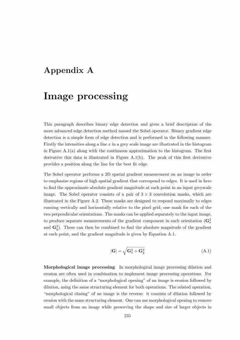
Appendix A
Image processing
This paragraph describes binary edge detection and gives a brief description of themore advanced edge detection method named the Sobel operator. Binary gradient edgedetection is a simple form of edge detection and is performed in the following manner.Firstly the intensities along a line x in a grey scale image are illustrated in the histogramin Figure A.1(a) along with the continuous approximation to the histogram. The firstderivative this data is illustrated in Figure A.1(b). The peak of this first derivativeprovides a position along the line for the best fit edge.
The Sobel operator performs a 2D spatial gradient measurement on an image in orderto emphasize regions of high spatial gradient that correspond to edges. It is used in hereto find the approximate absolute gradient magnitude at each point in an input greyscaleimage. The Sobel operator consists of a pair of 3 × 3 convolution masks, which areillustrated in the Figure A.2. These masks are designed to respond maximally to edgesrunning vertically and horizontally relative to the pixel grid, one mask for each of thetwo perpendicular orientations. The masks can be applied separately to the input image,to produce separate measurements of the gradient component in each orientation (G2
x
and G2y). These can then be combined to find the absolute magnitude of the gradient
at each point, and the gradient magnitude is given by Equation A.1.
|G| =√
G2x + G2
y (A.1)
Morphological image processing In morphological image processing dilation anderosion are often used in combination to implement image processing operations. Forexample, the definition of a “morphological opening” of an image is erosion followed bydilation, using the same structuring element for both operations. The related operation,“morphological closing” of an image is the reverse: it consists of dilation followed byerosion with the same structuring element. One can use morphological opening to removesmall objects from an image while preserving the shape and size of larger objects in
235
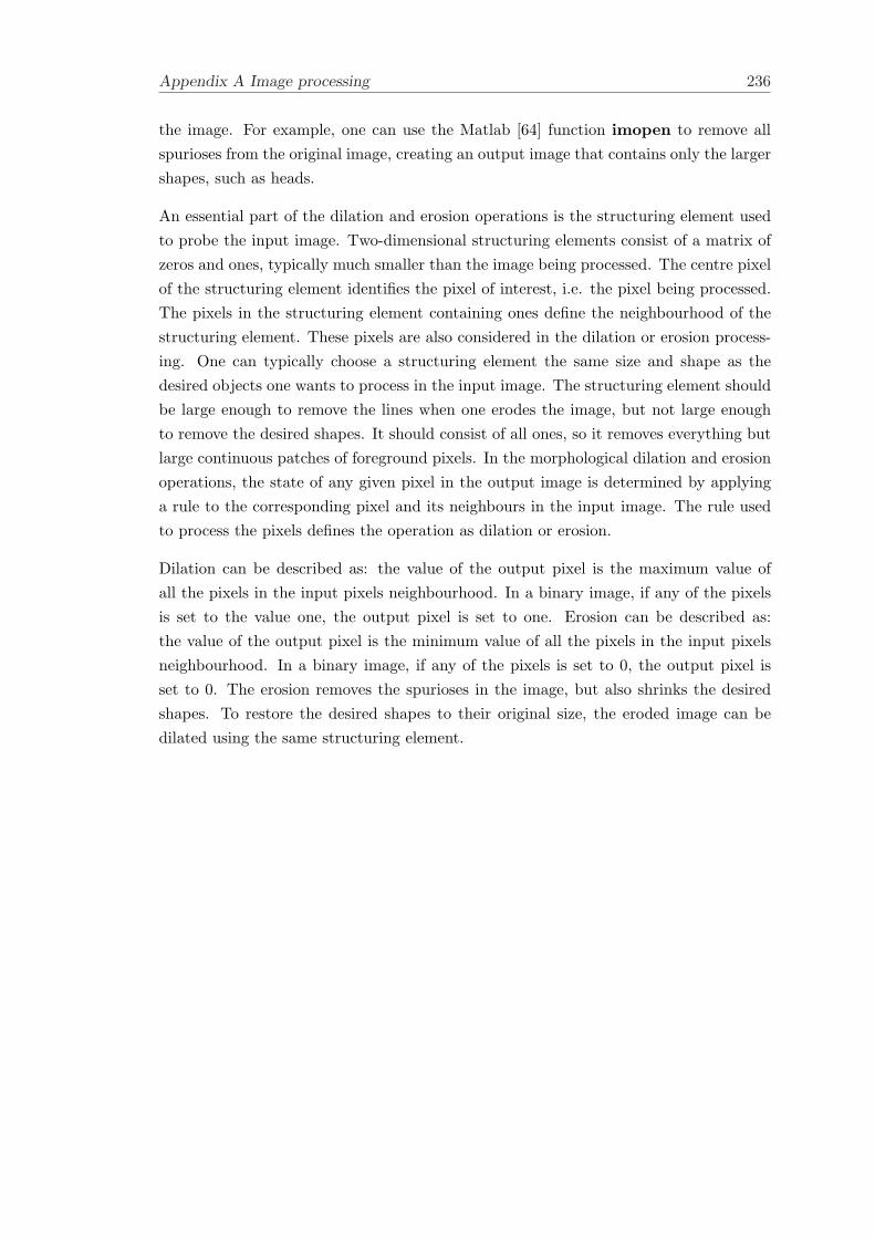
Appendix A Image processing 236
the image. For example, one can use the Matlab [64] function imopen to remove allspurioses from the original image, creating an output image that contains only the largershapes, such as heads.
An essential part of the dilation and erosion operations is the structuring element usedto probe the input image. Two-dimensional structuring elements consist of a matrix ofzeros and ones, typically much smaller than the image being processed. The centre pixelof the structuring element identifies the pixel of interest, i.e. the pixel being processed.The pixels in the structuring element containing ones define the neighbourhood of thestructuring element. These pixels are also considered in the dilation or erosion process-ing. One can typically choose a structuring element the same size and shape as thedesired objects one wants to process in the input image. The structuring element shouldbe large enough to remove the lines when one erodes the image, but not large enoughto remove the desired shapes. It should consist of all ones, so it removes everything butlarge continuous patches of foreground pixels. In the morphological dilation and erosionoperations, the state of any given pixel in the output image is determined by applyinga rule to the corresponding pixel and its neighbours in the input image. The rule usedto process the pixels defines the operation as dilation or erosion.
Dilation can be described as: the value of the output pixel is the maximum value ofall the pixels in the input pixels neighbourhood. In a binary image, if any of the pixelsis set to the value one, the output pixel is set to one. Erosion can be described as:the value of the output pixel is the minimum value of all the pixels in the input pixelsneighbourhood. In a binary image, if any of the pixels is set to 0, the output pixel isset to 0. The erosion removes the spurioses in the image, but also shrinks the desiredshapes. To restore the desired shapes to their original size, the eroded image can bedilated using the same structuring element.
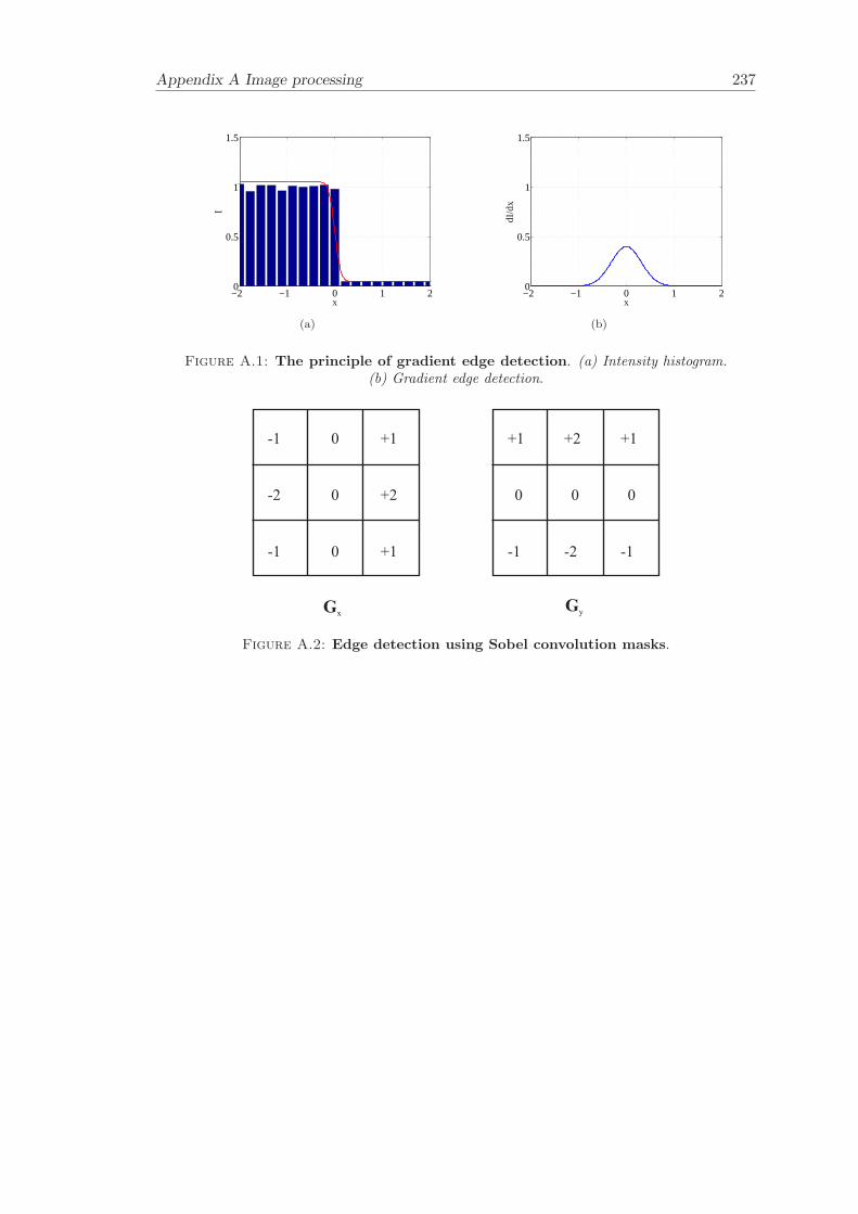
Appendix A Image processing 237
−2 −1 0 1 20
0.5
1
1.5
x
I
(a)
−2 −1 0 1 20
0.5
1
1.5
x
dI/d
x
(b)
Figure A.1: The principle of gradient edge detection. (a) Intensity histogram.(b) Gradient edge detection.
-1 0 +1 +1 +2 +1
-2
-1
0
0
+2
+1
0
-1
0
-2
0
-1
GxGy
Figure A.2: Edge detection using Sobel convolution masks.
Appendix B
Stereo vision
Disparity The disparity measure can be obtained by acquiring two images of thesame scene from different viewing positions. An estimation of the relative position of afeature as it appears in the two images makes it possible two calculate the distance ofthe feature, where the distance is between the baseline of the imaging devices and thefeature.
Figure B.1 illustrates the geometry of the stereo vision system in the horizontal plane.The principle is two cameras acquire two images of the same object from different view-points. The two viewpoints are noted as A and B and are the positions of the lensesof the two cameras. The distance between the viewpoints is the camera separation, andis noted as d. The point P (X,Y, Z) in the real world where the coordinate system hasan origin O, at the left camera (at point A). The X-direction is along the line betweenthe two lenses and the Y -direction is at right angles to X and parallel with the imageplanes. The focal length of the lenses is denoted by f . The distance from the imagecentre to the object are noted as xl and xr and the image centres are denoted by Ol andOr. The positions of P in the left and the right images are denoted by xl and xr withrespect to the local coordinate systems for each image (Ol and Or).
The disparity measure is calculated as follows. Firstly, using similar triangles in theX, Z-plane and in the X,Y -plane shows that a line from P through the centre of theleft camera lens intersects the Z = −f image plane. Similarly for the right camera, itfollows that
Xl = −Xof
ZoYl = −Yo
f
Zo(B.1)
Xr = −(Xo + d)f
ZoYr = −Yo
f
Zo= −Yo
f
Zo(B.2)
238
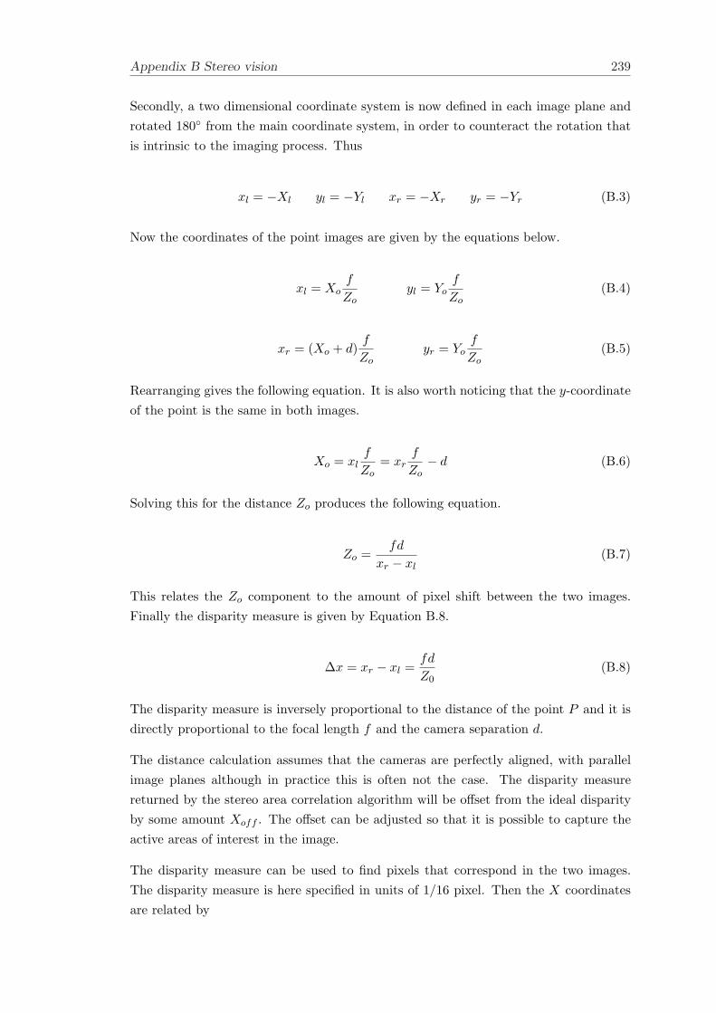
Appendix B Stereo vision 239
Secondly, a two dimensional coordinate system is now defined in each image plane androtated 180 from the main coordinate system, in order to counteract the rotation thatis intrinsic to the imaging process. Thus
xl = −Xl yl = −Yl xr = −Xr yr = −Yr (B.3)
Now the coordinates of the point images are given by the equations below.
xl = Xof
Zoyl = Yo
f
Zo(B.4)
xr = (Xo + d)f
Zoyr = Yo
f
Zo(B.5)
Rearranging gives the following equation. It is also worth noticing that the y-coordinateof the point is the same in both images.
Xo = xlf
Zo= xr
f
Zo− d (B.6)
Solving this for the distance Zo produces the following equation.
Zo =fd
xr − xl(B.7)
This relates the Zo component to the amount of pixel shift between the two images.Finally the disparity measure is given by Equation B.8.
∆x = xr − xl =fd
Z0(B.8)
The disparity measure is inversely proportional to the distance of the point P and it isdirectly proportional to the focal length f and the camera separation d.
The distance calculation assumes that the cameras are perfectly aligned, with parallelimage planes although in practice this is often not the case. The disparity measurereturned by the stereo area correlation algorithm will be offset from the ideal disparityby some amount Xoff . The offset can be adjusted so that it is possible to capture theactive areas of interest in the image.
The disparity measure can be used to find pixels that correspond in the two images.The disparity measure is here specified in units of 1/16 pixel. Then the X coordinatesare related by
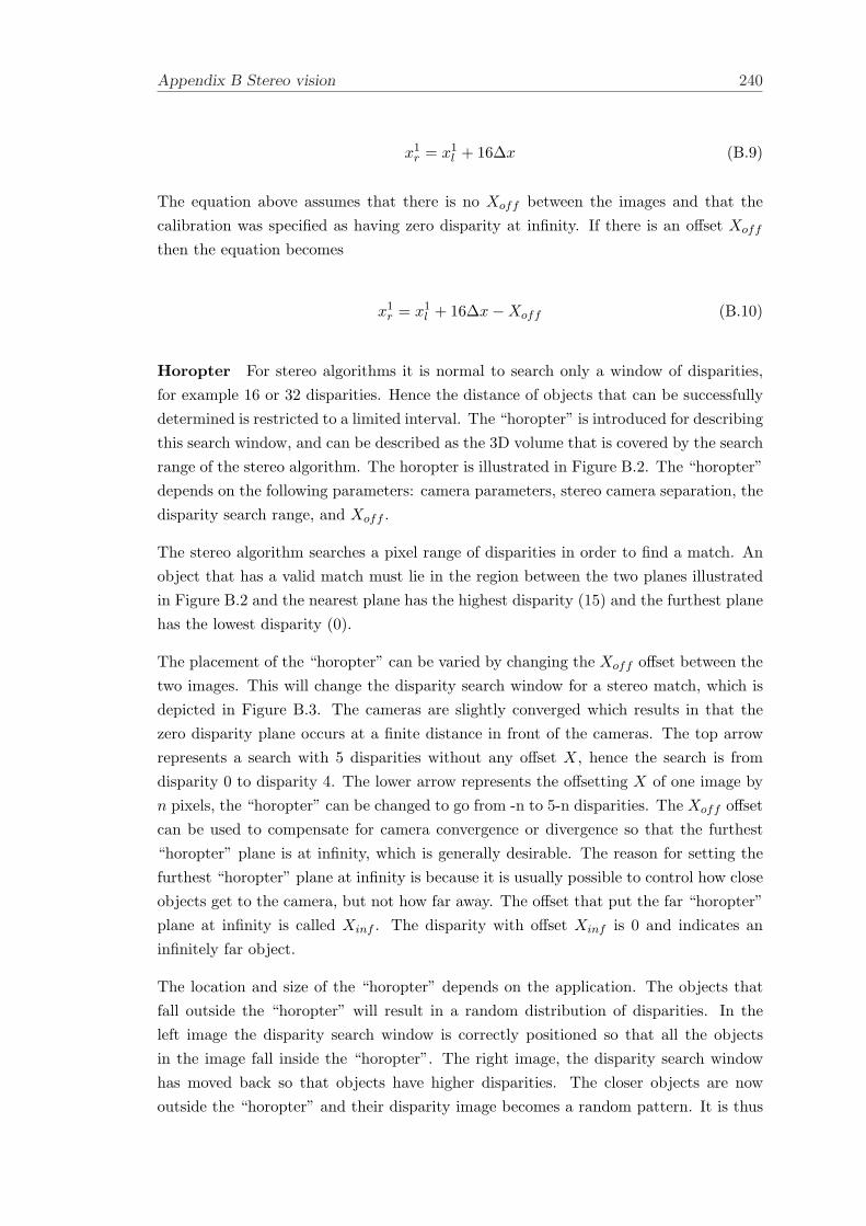
Appendix B Stereo vision 240
x1r = x1
l + 16∆x (B.9)
The equation above assumes that there is no Xoff between the images and that thecalibration was specified as having zero disparity at infinity. If there is an offset Xoff
then the equation becomes
x1r = x1
l + 16∆x−Xoff (B.10)
Horopter For stereo algorithms it is normal to search only a window of disparities,for example 16 or 32 disparities. Hence the distance of objects that can be successfullydetermined is restricted to a limited interval. The “horopter” is introduced for describingthis search window, and can be described as the 3D volume that is covered by the searchrange of the stereo algorithm. The horopter is illustrated in Figure B.2. The “horopter”depends on the following parameters: camera parameters, stereo camera separation, thedisparity search range, and Xoff .
The stereo algorithm searches a pixel range of disparities in order to find a match. Anobject that has a valid match must lie in the region between the two planes illustratedin Figure B.2 and the nearest plane has the highest disparity (15) and the furthest planehas the lowest disparity (0).
The placement of the “horopter” can be varied by changing the Xoff offset between thetwo images. This will change the disparity search window for a stereo match, which isdepicted in Figure B.3. The cameras are slightly converged which results in that thezero disparity plane occurs at a finite distance in front of the cameras. The top arrowrepresents a search with 5 disparities without any offset X, hence the search is fromdisparity 0 to disparity 4. The lower arrow represents the offsetting X of one image byn pixels, the “horopter” can be changed to go from -n to 5-n disparities. The Xoff offsetcan be used to compensate for camera convergence or divergence so that the furthest“horopter” plane is at infinity, which is generally desirable. The reason for setting thefurthest “horopter” plane at infinity is because it is usually possible to control how closeobjects get to the camera, but not how far away. The offset that put the far “horopter”plane at infinity is called Xinf . The disparity with offset Xinf is 0 and indicates aninfinitely far object.
The location and size of the “horopter” depends on the application. The objects thatfall outside the “horopter” will result in a random distribution of disparities. In theleft image the disparity search window is correctly positioned so that all the objectsin the image fall inside the “horopter”. The right image, the disparity search windowhas moved back so that objects have higher disparities. The closer objects are nowoutside the “horopter” and their disparity image becomes a random pattern. It is thus
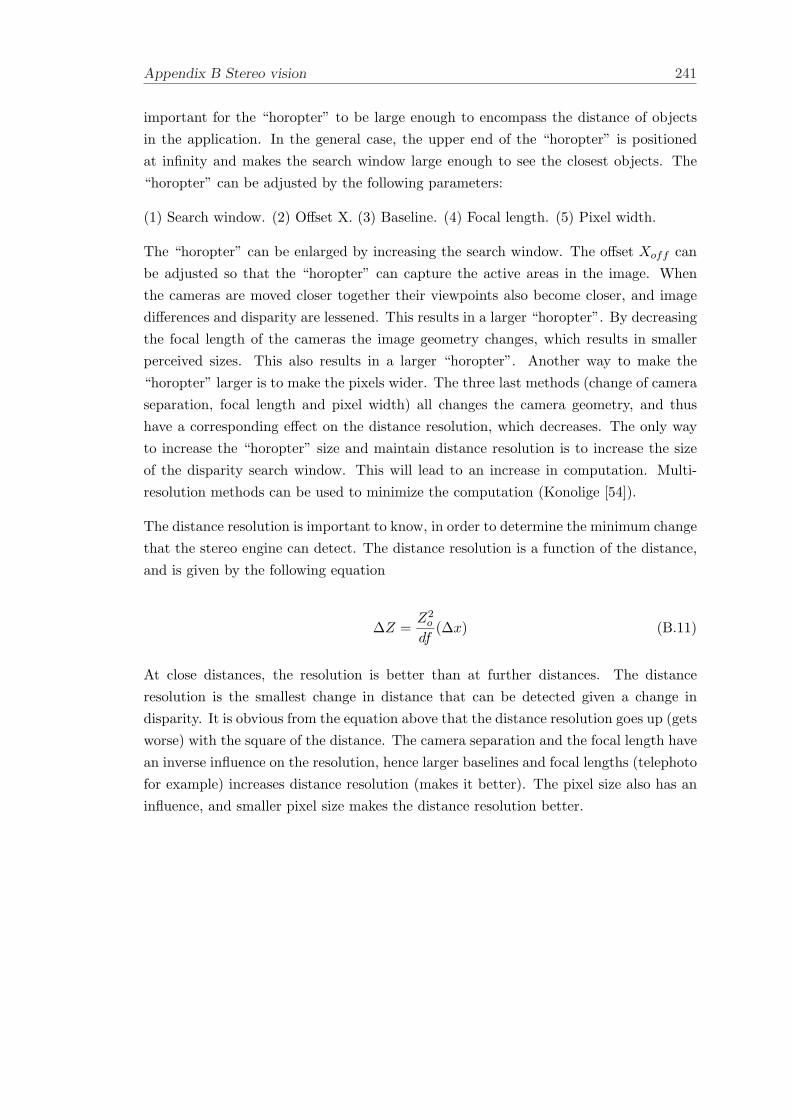
Appendix B Stereo vision 241
important for the “horopter” to be large enough to encompass the distance of objectsin the application. In the general case, the upper end of the “horopter” is positionedat infinity and makes the search window large enough to see the closest objects. The“horopter” can be adjusted by the following parameters:
(1) Search window. (2) Offset X. (3) Baseline. (4) Focal length. (5) Pixel width.
The “horopter” can be enlarged by increasing the search window. The offset Xoff canbe adjusted so that the “horopter” can capture the active areas in the image. Whenthe cameras are moved closer together their viewpoints also become closer, and imagedifferences and disparity are lessened. This results in a larger “horopter”. By decreasingthe focal length of the cameras the image geometry changes, which results in smallerperceived sizes. This also results in a larger “horopter”. Another way to make the“horopter” larger is to make the pixels wider. The three last methods (change of cameraseparation, focal length and pixel width) all changes the camera geometry, and thushave a corresponding effect on the distance resolution, which decreases. The only wayto increase the “horopter” size and maintain distance resolution is to increase the sizeof the disparity search window. This will lead to an increase in computation. Multi-resolution methods can be used to minimize the computation (Konolige [54]).
The distance resolution is important to know, in order to determine the minimum changethat the stereo engine can detect. The distance resolution is a function of the distance,and is given by the following equation
∆Z =Z2
o
df(∆x) (B.11)
At close distances, the resolution is better than at further distances. The distanceresolution is the smallest change in distance that can be detected given a change indisparity. It is obvious from the equation above that the distance resolution goes up (getsworse) with the square of the distance. The camera separation and the focal length havean inverse influence on the resolution, hence larger baselines and focal lengths (telephotofor example) increases distance resolution (makes it better). The pixel size also has aninfluence, and smaller pixel size makes the distance resolution better.
Appendix B Stereo vision 242
Left camera image
Right camera image
A
B
Xl
Xr
P X , Y , Z( )0 0 0
X
ZOl
Or
d
f
Figure B.1: The geometry of the stereo vision system viewed from above.
Plane ofclosest match
Plane offurthest match
16 disparities
Figure B.2: Horopter planes for disparity search.
Disparity: 5 4 3 2 1 0 -1 -2 -3
Figure B.3: Planes of constant disparity for a converged stereo camera. Asearch range of 5 pixels is shown to cover two different horopters, that depend on the
search offset X.
Appendix C
Condensation
The theory of the condensation algorithm is briefly described here. It is assumed thatthere are T frames of data to be processed and that at time t only data from times1, t− 1 are available. The measurements acquired from frame t are denoted Zt and willconsist of a list of edges observed in the image, as discussed in Section 7.4.3. The stateof the modelled object at time t is Yt. The measurements acquired up to frame t aredenoted Zt = Z1, ...Zt and the state of the modelled object up to frame t is denotedYt = Y1, ...Yt.
Dynamics The assumption that the object dynamics form a temporal Markov chainis made for the probabilistic framework, so that
p(Yt|Yt−1) = p(Yt|Yt−1) (C.1)
The new state is dependent only on the immediately preceding state and is indepen-dent of earlier states. The dynamics are now entirely determined by the form of theconditional density p(Yt|Yt−1).
Observations The observations Zt are assumed to be mutually independent and alsoindependent with respect to the dynamical process. The observation process is thereforedefined by specifying the observation density p(Zt|Yt) at each time t.
Propagation The conditional state-density at time t is defined by p(Yt|Zt) (assuminga continuous valued Markov-chain with independent observations). This represents allinformation about the state at time t that can be deduced from the entire data streamup to time t. The equation for propagation of state density over time is given by
243
Appendix C Condensation 244
p(Yt|Zt) = ktp(Zt|Yt)p(Yt|Zt−1) (C.2)
where
p(Yt|Zt−1) =∫
Yt−1
ktp(Yt|Yt−1)p(Yt−1|Zt−1)dYt−1 (C.3)
and kt is a normalisation constant that does not depend on Yt (this is proved by Is-ard [41]). The propagation of state density can be interpreted as Bayes’ theorem for in-ferring posterior state density from data, for the time varying case. The prior p(Yt|Zt−1)is a prediction taken from the posterior p(Yt−1|Zt−1) from the previous time step bysuperimposing one time-step from the dynamical model. The multiplication by the ob-servation density p(Zt|Yt) then applies the reactive effect expected from observations.Equation C.2 is the filter that the condensation algorithm must approximate.
Factored sampling This paragraph describes the factored sampling algorithm thatdeals with non-Gaussian observations in single images, which will be extended in thefollowing paragraph to deal with temporal image sequences.
Given a static image Z where the problem is to find an object parameterised as Y withprior p(Y). The posterior density p(Y|Z) represents all the knowledge about Y that isdeducible from the data. This can be evaluated by applying Bayes’ theorem:
p(Y|Z) = kp(Z|Y)p(Y) (C.4)
Where k is a normalisation constant that is independent of Y. When p(Z|Y) is suf-ficiently complex that p(Y|Z) cannot be evaluated in closed form, iterative samplingtechniques can be used (MacCormick [62]). The factored sampling algorithm generatesa random variate Y′ from the approximation of the posterior distribution denoted p(Y).First a sample set s(1), . . . , s(N) is generated from the prior density p(Y) and then eachindex i ∈ 1, . . . , N is assigned with probability πi , where
πi =pz(s(i))∑N
j=1 pz(s(j))(C.5)
pz(Y) = p(Z|Y) (C.6)
The index i determines the value Y′ = Yi and by choosing Y′ in this way gives ita distribution that approximates the posterior p(Y|Z) with increasing accuracy as N
increases. Moments of Y can be estimated using Equation C.7.
Appendix C Condensation 245
E[g(Y)|Z] =∑N
n=1 g(s(n))pz(s(n))∑Nn=1 pz(s(n))
(C.7)
The mean can be estimated by setting g(Y) = Y.
Summary of the algorithm The condensation algorithm uses factored samplingextended to apply iteratively to image sequences. The process at each time step is aniteration of factored sampling; and the output of an iteration will be a weighted, time-stamped sample set, denoted s(n)
t , n = 1, . . . , N with weights π(n)t , representing
approximately the conditional state density p(Yt|Zt) at time t. The process of obtainingthe sample set is described as follows: the process begins with an effective prior densityfor time step t denoted p(Yt|Zt−1) (which is multi-modal in general and no functionalrepresentation is available), this prior is derived from the sample set representations(n)
t−1, π(n)t−1 , n = 1, . . . , N of p(Yt−1|Zt−1) (the output from the previous time step),
to which the prediction must be applied.
The iterative process applied to sample sets is described in Figure C.1. At the top ofthe diagram, the output from time-step t− 1 is the weighted sample-sets(n)
t−1, π(n)t−1 , n = 1, . . . , N . The algorithm must have sample sets of fixed size N , so
that it can be guaranteed to run within a given computational resource. Therefore thefirst operation is to sample with replacement N times from the sample set s(n)
t−1, choosinga given element with probability π
(n)t−1. The elements with high weights may be chosen
several times, leading to identical copies of elements in the nth set. The elements withrelatively low weights may not be chosen at all. Each element chosen from the new setis now subjected to the predictive step. The motion model causes identical elementsto split and diffuse through state-space. Now the sample set s(n)
t for the new timestep has been generated but without its weights. It is approximately a random samplefrom the effective prior density p(Yt|Zt−1) for time step t. Finally the observation stepfrom factored sampling is performed, generating weights from the observation densityp(Zt|Yt), in order to obtain the sample set representation s(n)
t , π(n)t of the state density
for time t.
The condensation algorithm makes use of cumulative probabilities c(n)t calculated from
π(n)t :
c(n)t = 0
c(n)t = c
(n−1)t + π
(n)t (n = 1, . . . , N)
(C.8)
In step (1), a base sample s′(n)t = s(j)
t−1 is chosen from the sample set s(n)t−1, π
(n)t−1, c
(n)t−1
with probability π(j)t−1. This can be done by first generating a random number r ∈ [0, 1],
uniformly distributed, then find by binary subdivision the smallest j for which c(j)t−1 ≥ r
and finally set s′(n)t = s(j)
t−1.
Appendix C Condensation 246
After any time-step in the condensation algorithm, it is possible to report the currentstate, for example by evaluating moments of the state density.
The following provides a summary of the algorithm:
From the old sample set s(n)t−1, π
(n)t−1, c
(n)t−1 , n = 1, . . . , N at time step t− 1, construct
a new sample set s(n)t , π
(n)t , c
(n)t , n = 1, . . . , N and keep on iterating. Construct the
nth of new samples as follows:
(1) Select a sample s′(n)t = s(j)
t−1 with probability π(j)t−1 as discussed above.
(2) Predict by sampling from p(Yt|Yt−1 = s′(n)t ) to choose each s(n)
t . The new samplevalue is generated by applying the dynamics in equation 7.22.
(3) Measure and weight the new position in terms of the measured features Zt by usingπ
(n)t = p(Zt|Yt = s(n)
t ), then normalise so that∑
n π(n)t = 1 and store together with
cumulative probability as s(n)t , π
(n)t , c
(n)t
When the N samples have been constructed, one can then estimate moments of thetracked position at time-step t using the Minimum Mean Square Estimator (MMSE) as
E[f(Yt)] =∑N
n=1π
(n)t f(s(n)
t ) (C.9)
Where the mean position is obtained using f(Y) = Y.
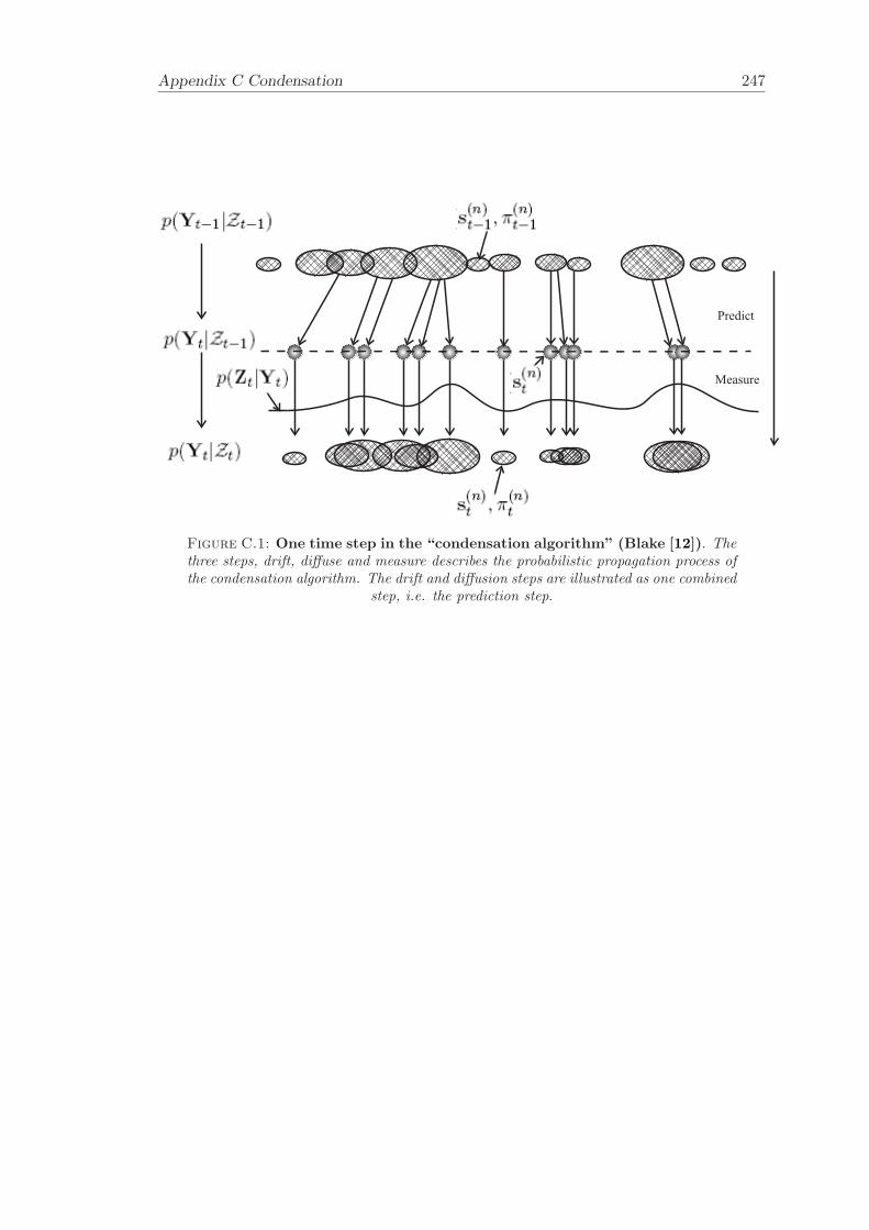
Appendix C Condensation 247
Predict
Measure
Figure C.1: One time step in the “condensation algorithm” (Blake [12]). Thethree steps, drift, diffuse and measure describes the probabilistic propagation process ofthe condensation algorithm. The drift and diffusion steps are illustrated as one combined
step, i.e. the prediction step.

Bibliography
[1] M. Abramowitz and I. A. Stegun. Handbook of Mathematical Functions. Dover,1965.
[2] V. Algazi, R. Duda, and D. Thompson. The cipic hrtf database. Technical report,CIPIC, 2001.
[3] V. Algazi, A. Ralph, C. Avendano, and R. Duda. Estimation of a spherical-headmodel from anthropometry. Journal of the Audio Engineering Society, 49:472–479,2001.
[4] B. S. Atal and M. R. Schroeder. Apparent sound source translater. US Patent,3,236,949, 1966.
[5] N. Ayache and P. T. Sander. Artificial Vision for Mobile Robots: Stereo Visionand Multisensory Perception. MIT Press, 1991.
[6] A. Azarbayejani, T. Darrell, and A. Pentland. Real-time tracking of the humanbody. Institute of Electrical and Electronics Engineers, Transactions on patternanalysis and machine intelligence, 19:780–785, 1997.
[7] A. Azarbayejani and A. Pentland. Real time self-calibrating stereo person trackingusing 3-d shape estimation from blob features. ICPR’96 Vienna, 1996.
[8] D. H. Ballard and C. M. Brown. Computer Vision. Prentice Hall, 1982.
[9] J. L. Bauck. A simple loudspeaker array and associated cross-talk canceller forimproved 3d audio. Journal of the Audio Engineering Society, 49:3–13, 2001.
[10] B. B. Bauer. Stereophonic earphones and binaural loudspeakers. Journal of theAudio Engineering Society, 9:148–151, 1961.
[11] D. R. Begault. 3-D Sound for Virtual Reality and Multimedia. Morgan KaufmannPub, 1994.
[12] A. Blake and M. Isard. Active Contours. Springer, 1998.
[13] J. Blauert. Spatial Hearing. The MIT Press, 2001.
248
BIBLIOGRAPHY 249
[14] M. A. Blommer and G. H. Wakefield. Pole-zero approximations for head-relatedtransfer functions using a logarithmic error criterion. Institute of Electrical andElectronics Engineers Transactions Speech Audio Processing, 5:278–287, 1997.
[15] R. Bowden. Learning Non-linear Models of Shape and Motion. Phd, Brunel Uni-versity, 1999.
[16] M. D. Burkard. Manikin measurements. Technical report, Knowles, 1978.
[17] K. R. Catleman. Digital Image Processing. Prentice Hall, 1996.
[18] J. Chen, B Van Veen, and K. Hecox. A spatial feature extraction and regularizationmodel for the head-related transfer function extraction. Journal of the AcousticalSociety of America, 97, 1995.
[19] D. H. Cooper and J. L. Bauck. Prospects for transaural recording. Journal of theAudio Engineering Society, 37:3–19, 1989.
[20] D. H. Cooper and J. L. Bauck. Generalised transaural stereo and applications.Journal of the Audio Engineering Society, 44:683–705, 1992.
[21] D. H. Cooper and J. L. Bauck. Head diffraction compensated stereo system withloudspeaker array. US Patent, 5,333,200, 1994.
[22] T. Cootes, G. J. Page, C. B. Jackson, and C. Taylor. Statistical grey-level mod-els for object location and identification. Proceedings of British Machine VisionConference, pages 533–542, 1995.
[23] R. Crochiere. Multirate Digital Processing. Prentice Hall, 1983.
[24] P. Damaske and V. Mellert. Sound reproduction of the upper semi-space withdirectional fidelity using two loudspeakers. Acoustica, 22:153–162, 1969.
[25] A. Doucet, N. Freitas, and N Gordon. Sequential Monte Carlo Methods in Practice.Springer, 2001.
[26] R. Duda and P. Hart. Pattern Classification and Scene Analysis. John Wiley andSons, 1973.
[27] E. A. Durant and G. H. Wakefield. Efficient model fitting using a genetic algorithm:Pole-zero approximations of hrtfs. Institute of Electrical and Electronics EngineersTransactions Speech Audio Processing, 1:18–27, 2002.
[28] M. Evans, J. Angus, and A. Tew. Analyzing head-related transfer function mea-surements using surface spherical harmonics. Journal of the Acoustical Society ofAmerica, 104, 1998.
BIBLIOGRAPHY 250
[29] A. Farina, G. Glasgal, E. Armelloni, and A. Torgers. Ambiophonic principles forthe recording and reproduction of surround sound for music. Audio EngineeringSociety 19th International Conference, 2001.
[30] W. G. Gardner. 3-D audio using loudspeakers. Phd thesis, MIT Media Laboratory,Cambridge, MA, 1997.
[31] W. G. Gardner and K. Martin. Hrtf measurement of a kemar dummy-head mi-crophone. Technical report, MIT Media Lab, 1994.
[32] G. H. Golub and C. F. Van Loan. Matrix computations. The John HoopkinsUniversity Press, Baltimore, MD, 1996.
[33] W. Grimson. Object recognition by computer. MIT press, 1990.
[34] S. R. Gunn. Dual Active Contour Models for Image Feature Extraction. Phd,University of Southampton, 1996.
[35] S. R. Gunn and M. S. Nixon. Snake head boundary extraction using local andglobal energy minimisation. Institute of Electrical and Electronics Engineers, Pro-ceedings of the International Conference on Pattern Recognition ICPR, B:581–585,1996.
[36] E. R. Hafter and C Trahiotis. Functions of the binaural system. Encyclopaedia ofAcoustic, 3:1461–1479, 1997.
[37] H. Hamada, N. Ikeshoji, Y. Ogura, and T. Miura. Relation between physical char-acteristics of orthostereophonc system and horizontal plane localization. Journalof the Acoustical Society of Japan, 6:143–154, 1996.
[38] J. Huopaniemi. VIRTUAL ACOUSTIC AND 3-D SOUND IN MULTIMEDIASIGNAL PROCESSING. PhD thesis, Helsinki University of Technology, 1999.
[39] J. Huopaniemi and M. Karjalainen. Comparison of digital filter design methodsfor 3-d sound. Institute of Electrical and Electronics Engineers, Nordic SignalProcessing Symposium (NORSIG96), Sep, 1996.
[40] IEEE. Programs for Digital Signal Processing. IEEE Press New York, 1979.
[41] M. Isard. Visual Motion Analysis by Probablistic Propagation of Conditional Den-sity. Phd, Oxford University, 1998.
[42] M. Jones and J. Rehg. Statistical color models with application to skin detection.Technical report, Cambridge Research Laboratory Compaq Computer CorporationOne Cambridge Center Massachusetts, 2002.
[43] J-M. Jot. Real-time spatial processing of sounds for music, multimedia and inter-active human-computer interfaces. Multimedia Systems, 7, 1999.
BIBLIOGRAPHY 251
[44] J-M. Jot, V. Larcher, and O. Warusfel. Digital signal processing issues in thecontext of binaural and transaural stereophony. Audio Engineering Society, Con-vention, 98:3980, 1995.
[45] M. Karjalainen, Piirila E., and Jarvinen A. Loudspeaker response equalisationusing warped digital filters. Proceedings of NorSig-96, pages 367–370, 1996.
[46] M. Kass, A. Witkin, and Terzopoulos P. Snakes: Active contour models. InProceedings 1st International Conference On Computer Vision, pages 259–268,1987.
[47] O. Kirkeby and P. A. Nelson. Local sound field reproduction using two closelyspaced loudspeakers. Journal of the Acoustical Society America, 104(3):1973–1981,1998.
[48] O. Kirkeby and P. A. Nelson. Digital filter design for inversion problems in soundreproduction. Journal of the Audio Engineering Society, 47, 1999.
[49] O. Kirkeby, P. A. Nelson, and H. Hamada. Stereo dipole - a virtual source imagingsystem using two closely spaced loudspeakers. Journal of the Audio EngineeringSociety, 46(5):387–395, 1998.
[50] O. Kirkeby, P. A. Nelson, H. Hamada, and F. Orduna-Bustamante. Fast deconvo-lution of multi-channel systems using regularisation. Proceedings - InternationalConference on Noise Control Engineering, (6):2829, 1996.
[51] O. Kirkeby, P. A. Nelson, F. Orduna-Bustamante, and H. Hamada. Local soundfield reproduction using digital signal processing. Journal of the Acoustical Societyof America, 100(3):1584, 1996.
[52] R. G. Klumpp and H. R. Eady. Some measurements of interaural time differencethresholds. Journal of Acoustic Society of America, 28:859–860, 1956.
[53] K. Konolige. Small vision systems: hardware and implementation. In EighthInternational Symposium on Robotics Research, pages 111–116, 1997.
[54] K. Konolige and D. Beymer. Sri small vision system, users manual. Technicalreport, SRI, 2004.
[55] P. Kuchi, P. Gabbur, P. Subbana, and S. David. Human face detection and trackingusing skin color modeling and connected component operators. Journal of theInstitution of Electronics and Telecommunication Engineers, 48:289–293, 2002.
[56] C. Kyriakakis, T. Holman, J Lim, H. Hong, and H. Neven. Signal processing,acoustics, and psychoacoustics for high quality desktop audio. Journal of VisualCommunication and Image Representation, 9:51–61, 1998.
BIBLIOGRAPHY 252
[57] T. I. Laakso, V. Valimaki, M. Karjalainen, and Laine U. K. Splitting the unitdelay. tools for fractional delay filter design. Institute of Electrical and ElectronicsEngineers Signal Processing Magazine, 13:30–60, 1996.
[58] T. Lentz and G. Behler. Dynamic cross-talk cancellation for binaural synthesis invirtual reality environments. Audio Engineering Society 117th Convention, 2004.
[59] T. Lentz and O. Schmitz. Realisation of an adaptive cross-calk cancellation systemfor a moving listener. Audio Engineering Society 21st Conference, 2002.
[60] T. Lentz, D. Schroder, M. Vorlander, and Assenmacher I. Virtual reality systemwith integrated sound field simulation and reproduction. EURASIP Journal onAdvances in Signal Processing, 2007.
[61] R. Y. Litovskya, S. H. Colburn, W. A. Yost, and S. J. Guzman. The precedenceeffect. Journal of the Acoustical Society of America, 104(4), 1999.
[62] J. MacCormick. Stochastic Algorithms for Visual Tracking. Springer, 2002.
[63] MathWorks. Signal processing toolbox user’s guide version 5, 2000.
[64] MathWorks. Image processing toolbox user’s guide version 5.1, 2005.
[65] MathWorks. Statistics toolbox user’s guide version 5.1, 2005.
[66] MathWorks. Matlab, the language of technical computing, r2007a, 2007.
[67] J. C. Middlebrooks. Narrow-band sound localization related to external earacoustics. Journal of Acoustical Society of America, (92):2607–2624, 1992.
[68] H. Moller. Fundamentals of binaural technology. Applied Acoustics, (0003), 1992.
[69] H. Moller, M. Sorensson, D. Hammershoi, and C. Jensen. Head related transferfunctions of human subjects. Audio Engineering Society, 43(5), 1995.
[70] B. C. Moore. An introduction to the Psychology of Hearing. Academic Press, 2003.
[71] P. A. Nelson. Active control for virtual acoustics. Proceeding of Active 2002: The2002 International Symposium on Active Control of Sound and Vibration, 1:67–89,2002.
[72] P. A. Nelson and S. J. Elliott. Active Control of Sound. Academic Press, London,1992.
[73] P. A. Nelson, H. Hamada, and S. J. Elliott. Adaptive inverse filters for stereophonicsound reproduction. Institute of Electrical and Electronics Engineers Transactionson Acoustics, Speech and Signal Processing, 40:1621–1632, 1992.
BIBLIOGRAPHY 253
[74] P. A. Nelson, O. Kirkeby, and H. Hamada. Local sound field reproduction usingtwo closely spaced loudspeakers. Journal of the Acoustical Society of America.,104:1973–1981, 1998.
[75] P. A. Nelson, F. Orduna-Bustamante, and D. Engler. Multi-channel signal process-ing techniques in the reproduction of sound. Journal of the Audio EngineeringSociety, 44:973–989, 1996.
[76] P. A. Nelson and J. F. W. Rose. The time domain response of some systems forsound reproduction. Journal of Sound and Vibration, 296:461–493, 2006.
[77] G. Neu, E. Mommertz, and A. Shmitz. Investigateions on true directional soundreproduction by playing head-referred recording over two loudspeakers. Acoustica76, 76:183–192 (In German), 1992.
[78] A. Neumaier and T. Schneider. Estimation of parameters and eigenmodes ofmultivariate autoregressive models. ACM transactions on Mathematical Software,27:25–57, 2001.
[79] S. G. Norcross, G. A. Souldre, and Lavoie M. C. Subjective investigations ofinverse filtering. Journal of the Audio Engineering Society, 52, 2004.
[80] A. V. Oppenheim and W. Schafer, R. Discrete Time Signal Processing. PrenticeHall, NJ, 1989.
[81] N. Otsu. A threshold selection method from gray-level histograms. Institute ofElectrical and Electronics Engineers: Transactions Systems, Man and Cybernetics,9:62–66, 1979.
[82] T. Papadopoulos and P. A. Nelson. The effectiveness of cross-talk cancellation andequalisation of electroacoustic plants in virtual acoustic imaging systems. Proceed-ings of the Institute of Acoustics, page 26(2), 2004.
[83] A. D. Pierce. Acoustics, An Introduction to Its Physical Principles and Applica-tions. Acoustical Society of America - American Institute of Acoustics, 1994.
[84] J. G. Proakis and D. G. Manolakis. Digital signal processing principles, algorithms,and applications. New York, Macmillan, 1992.
[85] Lord. Rayleigh. On our perception of sound direction. Philosophical magazine,13:214–232, 1907.
[86] J. Rose. A Visually Adaptive Virtual Sound Imaging System. Phd, University ofSouthampton, 2003.
[87] J. Rose, P. A. Nelson, B. Rafaely, and T. Takeuchi. Sweet spot size of virtualacoustic imaging systems at asymmetric listener locations. Journal of the Acousti-cal Society of America, 112(5 I):1992–2002, 2002.
BIBLIOGRAPHY 254
[88] L. Savioja, J. Huopaniemi, T. Lokki, and R. Vaananen. Creating interactive virtualacoustic environments. Journal of the Audio Engineering Society, 47:675–705,1999.
[89] T. Schneider and A. Neumaier. A matlab package for the estimation of parame-ters and eigenmodes of multivariate autoregressive models. ACM transactions onMathematical Software, 27:58–65, 2001.
[90] L. Sigal, S. Sclaroff, and V Athitsos. Skin color-based video segmentation undertime-varying illumination. Technical report, Boston University Computer Science,2003.
[91] J. S. Soo and K. K. Pang. Multidelay block frequency adaptive filter. IEEETransactions Acoutics, Speech, and Signal Processing, 38, 1990.
[92] T. G. Stockham Jr. High speed convolution and correlation. AFIPS Procedings1966 Spring Joint Computer Conference, 28:229–233, 1966.
[93] M. Storring, T. Kocka, H. Andersen, and E. Granum. Tracking regions of humanskin through illumination changes. Technical report, Computer Vision and MediaTechnology Laboratory, Aalborg University., 2003.
[94] M. Subbarao. Interpretation of Visual Motion: A Computational Study. PitmanPublishing, London, 1988.
[95] T. Takeuchi. Systems for virtual acoustic imaging using the binaural principle.PhD thesis, University of Southampton, 2001.
[96] T. Takeuchi and P. A. Nelson. Robustness to head misalignment of virtual acousticimaging systems. Journal of the Acoustical Society of America, 109:958–971, 2001.
[97] T. Takeuchi and P. A. Nelson. Optimal source distribution for binaural synthesisover loudspeakers. Journal of the Acoustical Society of America, 112:2786–2797,2002.
[98] A. Torger and A. Farina. Real-time partitioned convolution for ambiophonics andsurround. IEEE Workshop on Applications of Signal Processing to Audio andAcoustics, 2001.
[99] V. Valimaki and T. Laksoo. Suppression of transients in variable recursive digitalfilters with a novel and efficeint cancellation method. IEEE Transactions on SignalProcessing, 46:3408–3414, 1998.
[100] D. Ward and G. Elko. Optimum loudspeaker spacing for robust cross-talk can-cellation. Institute of Electrical and Electronics Engineers, Proceedings of the In-ternational Conference on Acoustics, Speech, and Signal Processing, 1:3514–3544,1998.


