Visualization of the Autonomous Systems Interconnections with HERMES

Visualization of the Autonomous SystemsInterconnections with Hermes?

Andrea Carmignani, Giuseppe Di Battista, Walter Didimo,Francesco Matera, and Maurizio Pizzonia

Dipartimento di Informatica e Automazione,Universita di Roma Tre, via della Vasca Navale 79,

00146 Roma, Italy.{carmigna,gdb,didimo,matera,pizzonia}@dia.uniroma3.it

Abstract. Hermes is a system for exploring and visualizing Autono-mous Systems and their interconnections. It relies on a three-tiers archi-tecture, on a large repository of routing information coming from hete-rogeneous sources, and on sophisticated graph drawing engine. Such anengine exploits static and dynamic graph drawing techniques.

1 Introduction and Overview

Computer networks are an endless source of problems and motivations for theGraph Drawing and for the Information Visualization communities. Several sy-stems aim at giving a graphical representation of computer networks at differentabstraction levels and for different types of users. To give only some examples(an interesting survey can be found in [17]):

1. Application level: Visualization of Web sites structures, Web maps [18,16],and Web caches [10].

2. Network level: Visualization of multicast backbones [22], internet traffic [23],routes, and interconnection of routers.

3. Data Link level: interconnection of switches and repeaters in a local areanetwork [1].

We deal with the problem of exploring and visualizing the interconnectionsbetween Autonomous Systems. An Autonomous System (in the following AS) isa group of networks under a single administrative authority. Roughly speaking,an AS can be seen as a portion of Internet, and Internet can be seen as thetotality of the ASes and their interconnections. Each AS is identified by aninteger number.

A route is a path on the network that can be used to reach a specific set of(usually contiguous) IP addresses. A route is described by its IP addresses, itscost, and by the set of ASes that are traversed. Routes are “announced” from an? Research supported in part by the Murst Project: “Algorithms for Large Data Sets”.

Hermes is presented at http://www.dia.uniroma3.it/∼hermes.

J. Marks (Ed.): GD 2000, LNCS 1984, pp. 150–163, 2001.c© Springer-Verlag Berlin Heidelberg 2001

Visualization of the Autonomous Systems Interconnections with Hermes 151

AS with messages like “through me you can reach a certain set of IP addresses,with a certain cost and traversing a certain set of other ASes”.

In order to exchange route’s information, the ASes adopt a network proto-col called BGP (Border Gateway Protocol) [31]. Such a protocol is based on adistributed architecture where border routers that belong to distinct adjacentASes exchange information about the routes they know. The exchange of routinginformation between ASes is subject to routing policies; for example an AS cansay “I do not want to be traversed by packets going to a certain other AS”.

Several tools have been developed for analyzing and visualizing the Internettopology at the ASes level [9,12,23,30]. However, in our opinion, such tools arestill not completely satisfactory both in the interaction with the user and inthe effectiveness of the drawings. Some of them have the goal of showing largeportions of Internet, but the maps they produce can be difficult to read (seee.g. [9]). Other tools point the attention on a specific AS, only showing that ASand its direct connections (see e.g. [23]).

In this work we describe a new system, called Hermes, which allows to getseveral types of information on a specific AS and to explore and visualize theASes interconnections. The main features of Hermes are the following.

Hermes has a three tiers architecture. The user interacts with a top-tierclient which collects the user requests and forwards them to a middle-tier server.The server translates the requests into queries to a repository (the bottom tier).With the top-tier the user can explore and visualize the ASes interconnections,and several information about ASes and the BGP routing policies. The userinteracts with a subgraph (called map) of the graph of all ASes interconnections.Each exploration step enriches the map with new ASes and connections (verticesand edges).

Hermes handles a large repository (about 50 MB). The repository is updatedoff-line from a plurality of sources [24]: APNIC, ARIN, BELL, CABLE&WIRE,CANET, MCI, RADB, RIPE, VERIO. The data in the repository are used fromHermes to construct the ASes interconnection graph.

The middle-tier server of Hermes encapsulates a graph drawing module thatcomputes the drawing of the ASes interconnections already explored at a specifictime. Such a module is based on the GDToolkit library [21] and has the followingmain features:

– Its basic drawing convention is the podevsnef [20] model for orthogonal dra-wings having vertices of degree greater than four. However, since the handledgraphs have often many vertices (ASes) of degree one connected with thesame vertex, the podevsnef model is enriched with new features for repre-senting such vertices.

– It is equipped with two different graph drawing algorithms. In fact, at eachexploration step the map is enriched and hence it has to be redrawn. Depen-ding on the situation, the system (or the user) might want to use a staticor a dynamic algorithm. Of course, the dynamic and the static algorithmshave advantages and drawbacks. The dynamic algorithm allows to preservethe mental map of the user [19,27] but can lead, after a certain number of

152 A. Carmignani et al.

exploration steps, to drawings that are less readable than those constructedwith a static algorithm.

– The static algorithm is based on the topology-shape-metrics approach [14]and exploits recent compaction techniques that can draw vertices with anyprescribed size [13]. The topology-shape-metrics approach has been shownto be very effective and reasonably efficient in practical applications [15].

– The dynamic algorithm is a new dynamic graph drawing algorithm that hasbeen devised according to three main constraints. (1) It had to be comple-tely integrated within the topology-shape-metrics approach in such a wayto be possible to alternate its usage with the usage of the static algorithm.(2) It had to be consistent with the variation of the podevsnef model usedby Hermes. (3) It had to allow vertices of arbitrary size. Several algorithmshave been recently proposed in the literature on dynamic graph drawingalgorithms. In [4] a linear time algorithm for orthogonal drawings is presen-ted, where the position of the vertices cannot be changed after the initialplacement. In [29] four different scenarios for interactive orthogonal graphdrawings are studied. Each scenario defines the changes allowed in the com-mon part of two consecutive drawings. In [7] it is described an interactiveversion of Giotto [33]; it allows to incrementally add vertices and edges toan orthogonal drawing so that the shape of the common part of two consecu-tive drawings is preserved and the number of bends is minimized under thisconstraint. In [5] it is presented a dynamic algorithm for orthogonal drawingsthat allows to specify the relative importance of the number of bends vs. thenumber of changes between two consecutive drawings. Other algorithms forconstructing drawings of graphs incrementally, while preserving the mentalmap of the user, are for example [26,11,28]. Also, in [6] it is presented astudy on different metrics that can be used to evaluate the changes betweendrawings in an interactive scenario. However, as far as we know, none of thecited dynamic algorithms enforces all the constraints (1)–(3).

The paper is organized as follows. In Section 2 we explain how the user inter-acts with Hermes and provide a high level description of the functionalities ofthe system. In Section 3 we give some details about the three tiered architectureof Hermes. Section 4 shows the results of a study on the ASes interconnectiongraph we have performed before choosing the graph drawing algorithms to ap-ply in Hermes. In particular we give measures on the local density and on theaverage degree of the vertices. In Section 5 we describe the drawing conventionand the algorithms.

2 Using Hermes

The user interacts with Hermes through an ASes subgraph. An ASes subgraph(also called map) is a subgraph of the graph of all ASes and their interconnec-tions. A map is initially constructed using two possible starting primitives. ASselection: An AS is chosen. The obtained map consists of such an AS plus all


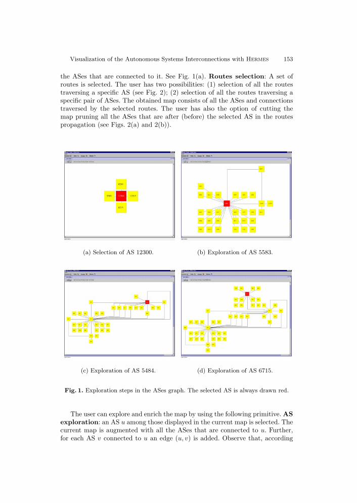
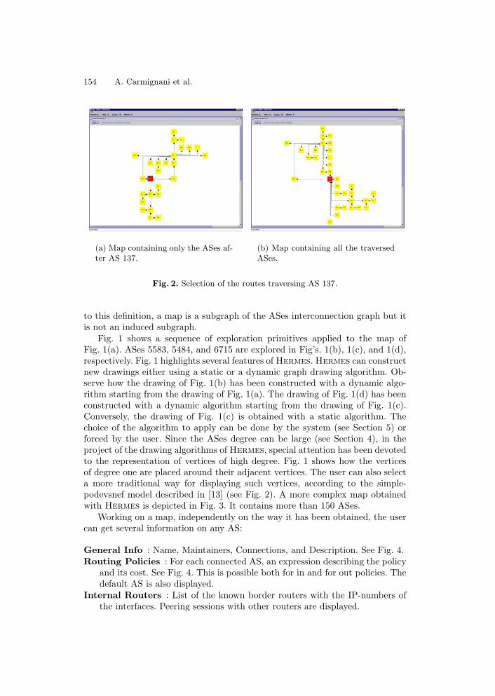
the ASes that are connected to it. See Fig. 1(a). Routes selection: A set ofroutes is selected. The user has two possibilities: (1) selection of all the routestraversing a specific AS (see Fig. 2); (2) selection of all the routes traversing aspecific pair of ASes. The obtained map consists of all the ASes and connectionstraversed by the selected routes. The user has also the option of cutting themap pruning all the ASes that are after (before) the selected AS in the routespropagation (see Figs. 2(a) and 2(b)).

(a) Selection of AS 12300. (b) Exploration of AS 5583.

(c) Exploration of AS 5484. (d) Exploration of AS 6715.

Fig. 1. Exploration steps in the ASes graph. The selected AS is always drawn red.

The user can explore and enrich the map by using the following primitive. ASexploration: an AS u among those displayed in the current map is selected. Thecurrent map is augmented with all the ASes that are connected to u. Further,for each AS v connected to u an edge (u, v) is added. Observe that, according


(a) Map containing only the ASes af-ter AS 137.

(b) Map containing all the traversedASes.

Fig. 2. Selection of the routes traversing AS 137.

to this definition, a map is a subgraph of the ASes interconnection graph but itis not an induced subgraph.

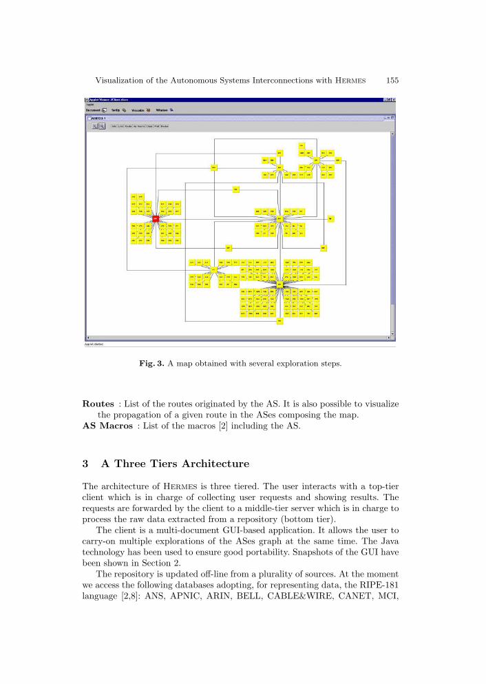
Fig. 1 shows a sequence of exploration primitives applied to the map ofFig. 1(a). ASes 5583, 5484, and 6715 are explored in Fig’s. 1(b), 1(c), and 1(d),respectively. Fig. 1 highlights several features of Hermes. Hermes can constructnew drawings either using a static or a dynamic graph drawing algorithm. Ob-serve how the drawing of Fig. 1(b) has been constructed with a dynamic algo-rithm starting from the drawing of Fig. 1(a). The drawing of Fig. 1(d) has beenconstructed with a dynamic algorithm starting from the drawing of Fig. 1(c).Conversely, the drawing of Fig. 1(c) is obtained with a static algorithm. Thechoice of the algorithm to apply can be done by the system (see Section 5) orforced by the user. Since the ASes degree can be large (see Section 4), in theproject of the drawing algorithms of Hermes, special attention has been devotedto the representation of vertices of high degree. Fig. 1 shows how the verticesof degree one are placed around their adjacent vertices. The user can also selecta more traditional way for displaying such vertices, according to the simple-podevsnef model described in [13] (see Fig. 2). A more complex map obtainedwith Hermes is depicted in Fig. 3. It contains more than 150 ASes.

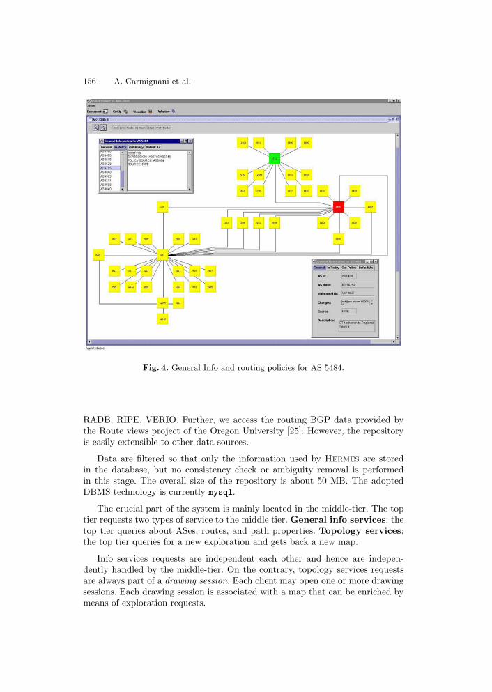
Working on a map, independently on the way it has been obtained, the usercan get several information on any AS:

General Info : Name, Maintainers, Connections, and Description. See Fig. 4.Routing Policies : For each connected AS, an expression describing the policy

and its cost. See Fig. 4. This is possible both for in and for out policies. Thedefault AS is also displayed.

Internal Routers : List of the known border routers with the IP-numbers ofthe interfaces. Peering sessions with other routers are displayed.


Fig. 3. A map obtained with several exploration steps.

Routes : List of the routes originated by the AS. It is also possible to visualizethe propagation of a given route in the ASes composing the map.

AS Macros : List of the macros [2] including the AS.

3 A Three Tiers Architecture

The architecture of Hermes is three tiered. The user interacts with a top-tierclient which is in charge of collecting user requests and showing results. Therequests are forwarded by the client to a middle-tier server which is in charge toprocess the raw data extracted from a repository (bottom tier).

The client is a multi-document GUI-based application. It allows the user tocarry-on multiple explorations of the ASes graph at the same time. The Javatechnology has been used to ensure good portability. Snapshots of the GUI havebeen shown in Section 2.

The repository is updated off-line from a plurality of sources. At the momentwe access the following databases adopting, for representing data, the RIPE-181language [2,8]: ANS, APNIC, ARIN, BELL, CABLE&WIRE, CANET, MCI,


Fig. 4. General Info and routing policies for AS 5484.

RADB, RIPE, VERIO. Further, we access the routing BGP data provided bythe Route views project of the Oregon University [25]. However, the repositoryis easily extensible to other data sources.

Data are filtered so that only the information used by Hermes are storedin the database, but no consistency check or ambiguity removal is performedin this stage. The overall size of the repository is about 50 MB. The adoptedDBMS technology is currently mysql.

The crucial part of the system is mainly located in the middle-tier. The toptier requests two types of service to the middle tier. General info services: thetop tier queries about ASes, routes, and path properties. Topology services:the top tier queries for a new exploration and gets back a new map.

Info services requests are independent each other and hence are indepen-dently handled by the middle-tier. On the contrary, topology services requestsare always part of a drawing session. Each client may open one or more drawingsessions. Each drawing session is associated with a map that can be enriched bymeans of exploration requests.


Info services requests are directly dispatched to a mediator. The mediatormodule is in charge to retrieve the data from the repository and to removeambiguities on-the-fly.

Topology services requests are handled by the kernel of the system. It getsinformation from the mediator and inserts new edges and vertices into the map.The drawing is computed by the drawing engine module (see Section 5). Thedrawing engine encapsulates GDToolkit [21].

4 AS Interconnection Data from a Graph DrawingPerspective

In order to devise effective graph drawing facilities for Hermes, we have analyzedthe ASes and their interconnections considering them as a unique large graphG. The data at our disposal show the following structure for G.

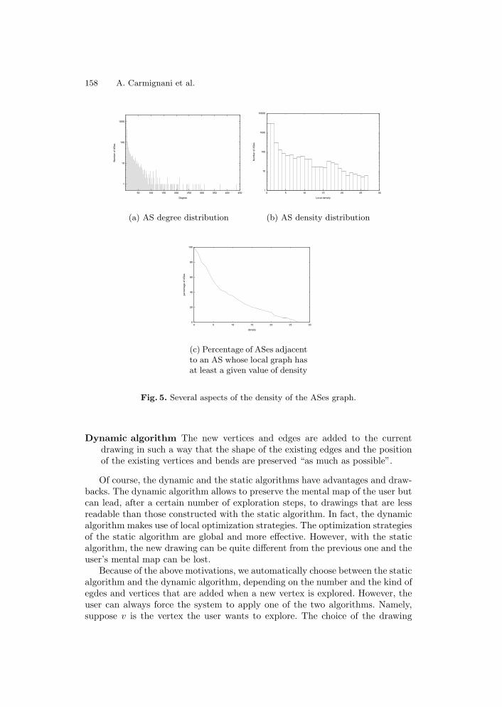
The number of vertices of G is 6, 849, while the number of edges is 27, 686.Fig. 5(a) illustrates the distribution of the degree of the vertices. The figure showsthat while there are many vertices (about 75%) with degree less or equal than4, there are also several vertices whose degree is more than 100. For improvingthe readability of the chart, we have omitted two vertices with degree 862 and1, 044, respectively. Further, consider that G contains 473 isolated vertices.

The density of G is 4.04. However, the “local” density can be much greater.In order to estimate such a local density, we have computed, for each vertex v,the density of the subgraph induced by the vertices adjacent to v. We call suchgraphs local graphs. Fig. 5(b) illustrates the distribution of the densities of thelocal graphs. From the figure it is possible to observe that about 5% of the localgraphs have density greater than 10.

We have also tried to estimate the probability, for a user that explores G, toencounter a portion of G that is locally dense. Fig. 5(c) shows, for each value dof density, what is the percentage of vertices that are adjacent to a vertex whoselocal graph has density at least d. Note that more than 30% of the vertices areadjacent to a vertex whose local graph has density at least 10.

Concerning connectivity, the graph has 480 connected components, includingthe above mentioned 473 isolated vertices. One of them has 6, 360 vertices; eachof the remaining 6 components has less than 6 vertices.

5 Drawing Conventions and Algorithmic Issues

At each exploration step, Hermes computes a new drawing. Namely, when theuser selects in the map a new vertex v, all the vertices and edges connected tov are added to the map, and such a map is redrawn. We use, depending on thespecific situation, two different drawing algorithms.

Static algorithm The current map is completely redrawn, after the new ver-tices and edges have been added.


1

10

100

1000

50 100 150 200 250 300 350 400 450

Num

ber

of A

Ses

Degree

(a) AS degree distribution

1

10

100

1000

10000

0 5 10 15 20 25 30

Num

ber

of A

Ses

Local density

(b) AS density distribution

0

20

40

60

80

100

0 5 10 15 20 25 30

perc

enta

ge o

f AS

es

density

(c) Percentage of ASes adjacentto an AS whose local graph hasat least a given value of density

Fig. 5. Several aspects of the density of the ASes graph.

Dynamic algorithm The new vertices and edges are added to the currentdrawing in such a way that the shape of the existing edges and the positionof the existing vertices and bends are preserved “as much as possible”.

Of course, the dynamic and the static algorithms have advantages and draw-backs. The dynamic algorithm allows to preserve the mental map of the user butcan lead, after a certain number of exploration steps, to drawings that are lessreadable than those constructed with the static algorithm. In fact, the dynamicalgorithm makes use of local optimization strategies. The optimization strategiesof the static algorithm are global and more effective. However, with the staticalgorithm, the new drawing can be quite different from the previous one and theuser’s mental map can be lost.

Because of the above motivations, we automatically choose between the staticalgorithm and the dynamic algorithm, depending on the number and the kind ofegdes and vertices that are added when a new vertex is explored. However, theuser can always force the system to apply one of the two algorithms. Namely,suppose v is the vertex the user wants to explore. The choice of the drawing


algorithm to apply is done by calculating an exploration cost for v and comparingsuch a cost with a treshold that can be set-up in a configuration menu. Theexploration cost is computed as follows. For any new edge the cost is 1. For anyvertex that had degree 1 in the old graph and whose degree is increased in thenew graph the cost is 0.5. An extra cost is also added as a function of the numberof times the dynamic algorithm has been invoked before. The exploration cost isa very rough estimate of the efficiency and effectiveness of the dynamic algorithmwith respect to the new exploration. The reason why vertices with degree 1 aretreated in a special way will be clear in the description of the algorithms.

The static algorithm we use consists of the following steps.

Degree-one Vertex Removal Vertices of degree one are temporarily remo-ved.

Planarization A standard planarization [14] technique is applied.Orthogonalization and Compaction We apply a variation of the techni-

que presented in [13] for constructing orthogonal drawings (in the simple-podavsnef model) with vertices of prescribed size. The box representing avertex v is a rectangle. Edges incident on v can incide the box only in themiddle points of the sides. The length of the sides are chosen in such away to have enough space to accommodate all the vertices that have beentemporarily removed in the first step and that were adjacent to v.

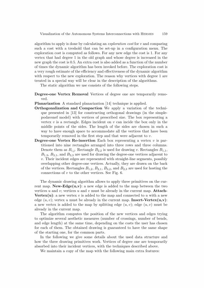
Degree-one Vertex Re-insertion Each box representing a vertex v is par-titioned into nine rectangles arranged into three rows and three columns.Denote them as Bi,j . Rectangle B2,2 is used for drawing v. Rectangles B1,1,B1,3, B3,1, and B3,3 are used for drawing the degree-one vertices adjacent tov. Their incident edges are represented with straight-line segments, possiblyoverlapping other degree-one vertices. Actually, they are drawn on the backof the vertices. Rectangles B1,2, B2,1, B3,2, and B2,3 are used for hosting theconnections of v to the other vertices. See Fig. 6.

The dynamic drawing algorithm allows to apply three primitives on the cur-rent map. New-Edge(u,v): a new edge is added to the map between the twovertices u and v; vertices u and v must be already in the current map. Attach-Vertex(u): a new vertex v is added to the map and connected to u with a newedge (u, v); vertex u must be already in the current map. Insert-Vertex(u,v):a new vertex is added to the map by splitting edge (u, v); edge (u, v) must bealready in the current map.

The algorithm computes the position of the new vertices and edges tryingto optimize several aesthetic measures (number of crossings, number of bends,and edge length) at the same time, depending on the costs the user has chosenfor each of them. The obtained drawing is guaranteed to have the same shapeof the starting one, for the common parts.

In the following we give some details about the used data structure andhow the three drawing primitives work. Vertices of degree one are temporarilyabsorbed into their incident vertices, with the techniques described above.

We maintain a copy of the map with the following main extra features:


B11 B13

B21 B23

B31 B33

B12

B22

B32

(a) (b)

Fig. 6. Using a box to represent a vertex. (a) The nine regions. (b) Using the nineregions to reinsert degree-one vertices.

– All the crossings and bends of the map are replaced by dummy vertices, sothat the topology of the drawing becomes planar.

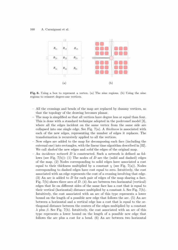
– The map is simplified so that all vertices have degree less or equal than four.This is done with a standard technique adopted in the podevsnef model [3],where all the edges incident on the same vertex from the same side arecollapsed into one single edge. See Fig. 7(a). A thickness is associated witheach of the new edges, representing the number of edges it replaces. Thetransformation is recursively applied to all the vertices.

– New edges are added to the map for decomposing each face (including theexternal one) into rectangles, with the linear time algorithm described in [32].We call dashed the new edges and solid the edges of the original map.

– An incidence network D is constructed. Such a network is defined as fol-lows (see Fig. 7(b)): (1) The nodes of D are the (solid and dashed) edgesof the map. (2) Nodes corresponding to solid edges have associated a costequal to their thickness multiplied by a constant χ (see Fig. 7(a)). Nodescorresponding to dashed edges have cost equal to zero. Intuitively, the costassociated with an edge represents the cost of a crossing involving that edge.(3) An arc is added to D for each pair of edges of the map sharing a face.Fig. 7(b) shows three arcs of D. (4) An arc between two horizontal (vertical)edges that lie on different sides of the same face has a cost that is equal totheir vertical (horizontal) distance multiplied by a constant λ. See Fig. 7(b).Intuitively, the cost associated with an arc of this type represents a lowerbound on the length of a possible new edge that follows the arc. (5) An arcbetween a horizontal and a vertical edge has a cost that is equal to the or-thogonal distance between the centers of the edges multiplied by a constantλ plus β. See Fig. 7(b). Intuitively, the cost associated with an arc of thistype represents a lower bound on the length of a possible new edge thatfollows the arc plus a cost for a bend. (6) An arc between two horizontal


(vertical) edges that lie on the same side of the same face has a cost thatis equal to the distance between the centers of the edges plus 2 (multipliedby a constant λ) plus 2β. See Fig. 7(b). Intuitively, the cost associated withan arc of this type represents a lower bound on the length of a possible newedge that follows the arc plus a cost for two bends. (7) Intuitively, χ, β,and λ, represent the costs for one cross, one bend, and one unit of length,respectively. Their values can be set-up by the user. The ratios between χ,β, and λ may determine different behaviors of the algorithm.

χχ4 3 χ χ2

(a) Collapsing the ed-ges incident on the sameside of a vertex.

d1d1λd2

3d 4d

4d2 +( )β2 +

3dd2 + )(β+ λ

λ

(b) Nodes (little squares) and arcs ofthe incidence network.

Fig. 7. Illustration of the dynamic algorithm.

Primitives New-Edge, Attach-Vertex, and Insert-Vertex are implemented asfollows.

New-Edge(u,v) : In the case u and v are not on the same face two temporarynodes are added to D representing u and v. Also, temporary arcs are addedto D between u and the nodes representing its incident edges. The same isdone for v. The temporary arcs have zero cost.A shortest path between u and v is computed. Such a path determines theroute and the shape of the new edge. Namely, the new edge is inserted in themap following the arcs of the shortest path. The temporary nodes and arcsare removed an the new faces originated by the new edge are decomposedinto rectangles.In the case u and v are on the same face a simpler technique (not discussedhere for brevity) is adopted.

Attach-Vertex(u) : A local evaluation of the edges incident on u is performed.The new edge is put preferably either on a direction around u where thereis no incident edge or on a dashed edge.

Insert-Vertex(u,v) : Edge (u, v) is just split into two pieces. If the edge has abend we put the new vertex preferably on that bend.


Once a primitive has been performed, the expansion technique describedabove is applied to make room for the vertices of degree one that were tempora-rily absorbed into their incident vertices.

Observe that D can have a number of arcs that is quadratic in the numberof edges of the map. However, it is possible to see that D can be simplified toan equivalent net with a linear number of arcs.

Acknowledgements. We are grateful to Sandra Follaro and Antonio Leon-forte for their fundamental contribution in the implementation of the dynamicalgorithm. We are also grateful to Andrea Cecchetti for useful discussion on therepository.

References

1. Aprisma. Spectrum. On line. http://www.aprisma.com.2. T. Bates, E. Gerich, L. Joncheray, J. M. Jouanigot, D. Karrenberg, M. Terpstra,

and J. Yu. Representation of ip routing policies in a routing registry. On line,1994. ripe-181, http://www.ripe.net, rfc 1786.

3. P. Bertolazzi, G. Di Battista, and W. Didimo. Computing orthogonal drawingswith the minimum numbr of bends. IEEE Transactions on Computers, 49(8), 2000.

4. T. C. Biedl and M. Kaufmann. Area-efficient static and incremental graph dar-wings. In R. Burkard and G. Woeginger, editors, Algorithms (Proc. ESA ’97),volume 1284 of Lecture Notes Comput. Sci., pages 37–52. Springer-Verlag, 1997.

5. U. Brandes and D. Wagner. Dynamic grid embedding with few bends and changes.In K.-Y. Chwa and O. H. Ibarra, editors, ISAAC’98, volume 1533 of Lecture NotesComput. Sci., pages 89–98. Springer-Verlag, 1998.

6. S. Bridgeman and R. Tamassia. Difference metrics for interactive orthogonal graphdrawing algorithms. In S. H. Withesides, editor, Graph Drawing (Proc. GD ’98),volume 1547 of Lecture Notes Comput. Sci., pages 57–71. Springer-Verlag, 1998.

7. S. S. Bridgeman, J. Fanto, A. Garg, R. Tamassia, and L. Vismara. Interactive-Giotto: An algorithm for interactive orthogonal graph drawing. In G. Di Battista,editor, Graph Drawing (Proc. GD ’97), volume 1353 of Lecture Notes Comput.Sci., pages 303–308. Springer-Verlag, 1998.

8. M. Bukowy and J. Snabb. RIPE NCC database documentation update to supportRIPE DB ver. 2.2.1. On line, 1999. ripe-189, http://www.ripe.net.

9. CAIDA. Otter: Tool for topology display. On line. http://www.caida.org.10. CAIDA. Plankton: Visualizing nlanr’s web cache hierarchy. On line.

http://www.caida.org.11. R. F. Cohen, G. Di Battista, R. Tamassia, and I. G. Tollis. Dynamic graph dra-

wings: Trees, series-parallel digraphs, and planar ST -digraphs. SIAM J. Comput.,24(5):970–1001, 1995.

12. Cornell University. Argus. On line.http://www.cs.cornell.edu/cnrg/topology aware/discovery/argus.html.

13. G. Di Battista, W. Didimo, M. Patrignani, and M. Pizzonia. Orthogonal andquasi-upward drawings with vertices of prescribed sizes. In J. Kratochvil, editor,Graph Drawing (Proc. GD ’99), volume 1731 of Lecture Notes Comput. Sci., pages297–310. Springer-Verlag, 1999.

14. G. Di Battista, P. Eades, R. Tamassia, and I. G. Tollis. Graph Drawing. PrenticeHall, Upper Saddle River, NJ, 1999.


15. G. Di Battista, A. Garg, G. Liotta, R. Tamassia, E. Tassinari, and F. Vargiu.An experimental comparison of four graph drawing algorithms. Comput. Geom.Theory Appl., 7:303–325, 1997.

16. G. Di Battista, R. Lillo, and F. Vernacotola. Ptolomaeus: The web cartographer.In S. H. Withesides, editor, Graph Drawing (Proc. GD ’98), volume 1547 of LectureNotes Comput. Sci., pages 444–445. Springer-Verlag, 1998.

17. M. Dodge. An atlas of cyberspaces. On line.http://www.cybergeography.com/atlas/atlas.html.

18. P. Eades, R. F. Cohen, and M. L. Huang. Online animated graph drawing for webnavigation. In G. Di Battista, editor, Graph Drawing (Proc. GD ’97), volume 1353of Lecture Notes Comput. Sci., pages 330–335. Springer-Verlag, 1997.

19. P. Eades, W. Lai, K. Misue, and K. Sugiyama. Preserving the mental map of adiagram. In Proceedings of Compugraphics 91, pages 24–33, 1991.

20. U. Foßmeier and M. Kaufmann. Drawing high degree graphs with low bend num-bers. In F. J. Brandenburg, editor, Graph Drawing (Proc. GD ’95), volume 1027of Lecture Notes Comput. Sci., pages 254–266. Springer-Verlag, 1996.

21. GDToolkit:. Graph drawing toolkit. On line. http://www.gdtoolkit.com.22. B. Huffaker. Tools to visualize the internet multicast backbone. On line.

http://www.caida.org.23. IPMA. Internet performance measurement and analysis project. On line.

http://www.merit.edu/ipma.24. Merit Network, Inc. Radb database services. On line. http://www.radb.net.25. D. Meyer. University of oregon route views project. On line.

http://www.antc.uoregon.edu/route-views.26. K. Miriyala, S. W. Hornick, and R. Tamassia. An incremental approach to aesthetic

graph layout. In Proc. Internat. Workshop on Computer-Aided Software Enginee-ring, 1993.

27. K. Misue, P. Eades, W. Lai, and K. Sugiyama. Layout adjustment and the mentalmap. J. Visual Lang. Comput., 6(2):183–210, 1995.

28. S. North. Incremental layout in DynaDAG. In F. J. Brandenburg, editor, GraphDrawing (Proc. GD ’95), volume 1027 of Lecture Notes Comput. Sci., pages 409–418. Springer-Verlag, 1996.

29. A. Papakostas and I. G. Tollis. Interactive orthogonal graph drawing. IEEETransactions on Computers, 47(11):1297–1309, 1998.

30. C. Rachit. Octopus: Backbone topology discovery. On line.http://www.cs.cornell.edu/cnrg/topology aware/topology/Default.html.

31. Y. Rekhter. A border gateway protocol 4 (bgp-4). IETF, rfc 1771.32. R. Tamassia. On embedding a graph in the grid with the minimum number of

bends. SIAM J. Comput., 16(3):421–444, 1987.33. R. Tamassia, G. Di Battista, and C. Batini. Automatic graph drawing and reada-

bility of diagrams. IEEE Trans. Syst. Man Cybern., SMC-18(1):61–79, 1988.

Documents

Visualization of the Autonomous Systems Interconnections with HERMES