Embed Size (px)
Citation preview
Vehicular Tra�c Noise Modelling of Urban Area- AContouring & Arti�cial Neural Network-BasedApproachAbhijit Debnath ( [email protected] )
Indian Institute of Technology BHU Varanasi https://orcid.org/0000-0002-4783-5174Prasoon Kumar Singh
IIT (ISM): Indian Institute of TechnologySushmita Banerjee
Sharda University
Research Article
Keywords: tra�c noise, tra�c �ow, noise descriptors, indexes, contour, ANN
Posted Date: November 15th, 2021
DOI: https://doi.org/10.21203/rs.3.rs-707329/v1
License: This work is licensed under a Creative Commons Attribution 4.0 International License. Read Full License
Version of Record: A version of this preprint was published at Environmental Science and PollutionResearch on February 3rd, 2022. See the published version at https://doi.org/10.1007/s11356-021-17577-1.
1
Vehicular Traffic Noise Modelling of Urban Area- A Contouring & Artificial Neural Network-Based 1
Approach 2
Abhijit Debnath 1*, Prasoon Kumar Singh 2, Sushmita Banerjee 3 3
1 2 Department of Environmental Sciencsuppe & Engineering, Indian Institute of Technology (ISM), Dhanbad, India 4
3 School of Basic Sciences and Research, Department of Environmental Sciences, Sharda University, Greater Noida, 5
India 6
2 3 Authors with equal contributions 7
* Corresponding author: Abhijit Debnath ( [email protected]) (ORCID: 0000-0002-4783-5174); Telephone: 8
+91-9612654872 9
10
Abstract: Road traffic vehicular noise is one of the main sources of environmental pollution in urban areas of India. 11
Also, steadily increasing urbanization, industrialization, infrastructures around city condition causing health risks 12
among the urban populations. In this study we have explored noise descriptors (L10, L90, Ldn, LNI, TNI, NC), contour 13
plotting and finds the suitability of artificial neural networks (ANN) for the prediction of traffic noise all around the 14
Dhanbad township in 15 monitoring stations. In order to develop the prediction model, measuring noise levels of five 15
different hours, speed of vehicles and traffic volume in every monitoring point have been studied and analyzed. Traffic 16
volume, percent of heavy vehicles, Speed, traffic flow, road gradient, pavement, road side carriageway distance factors 17
taken as input parameter, whereas LAeq as output parameter for formation of neural network architecture. As traffic 18
flow is heterogenous which mainly contains 59% 2-wheelers and different vehicle specifications with varying speeds 19
also effects driving and honking behavior which constantly changing noise characteristics. From radial noise diagrams 20
shown that average noise levels of all the stations beyond permissible limit and highest noise levels were found at the 21
speed of 50-55 km/h in both peak and non-peak hours. Noise descriptors clearly indicates high annoyance level in the 22
study area. Artificial neural network with 7-7-5 formation has been developed and found as optimum due to its sum 23
of square and overall relative error 0.858 & .029 in training and 0.458 & 0.862 in testing phase respectively. 24
Comparative analysis between observed and predicted noise level shows very less deviation up to ±0.6 dB(A) and the 25
R2 linear values are more than 0.9 in all five noise hours indicating the accuracy of model. Also, it can be concluded 26
that ANN approach is much superior in prediction of traffic noise level to any other statistical method. 27
Keywords: traffic noise; traffic flow; noise descriptors; indexes; contour; ANN 28
29
30
1 Present Address: Department of Civil Engineering, Indian Institute of Technology (BHU), Varanasi, India
2
31
Highlights: 32
1. Traffic noise level of all over the Dhanbad township area are beyond permissible limit in peak and non-peak 33
hours. 34
2. Study explores the contour noise plots w.r.t speed and volume, noise descriptors, finds suitability of ANN 35
modelling. 36
3. Noise descriptors indicates high annoyance level, a high degree of variation in traffic flow. 37
4. ANN model shows deviation up to ±0.6 dB(A) compared to measured levels and R2 linear values (goodness 38
of fit) are nearby best fit. 39
3
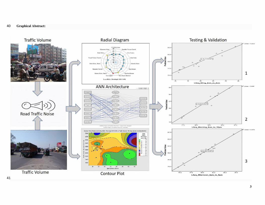
Graphical Abstract: 40
41
4
1.1 Introduction 42
Noise pollution is one of the major issues in urban environments which arises due to steady increase of 43
vehicular traffic in roads, urbanization, industrialization, and infrastructures around city conditions. Transportation 44
systems are an important feature of many developed societies, as transportation systems deliver the essential 45
infrastructure to ensure movement and convenience for societal needs (Di et al. 2018). 46
The world is experiencing an exponential rise in number of vehicles, leading to an rise in the traffic noise levels (Nedic 47
et al. 2014) and these levels results many health deprivation in residential and commercial areas such as sleep 48
problems, headaches, irritation, unusual tiredness (Huang et al. 2017). In Indian conditions, traffic noise mainly occurs 49
due to unnecessary horns as well as interaction between vehicle tires and road surface, engine noise etc. (Konbattulwar 50
et al. 2016). Vehicle horns are continuously honking in the road network system due to lack of proper traffic 51
management, high volume of vehicles, driver discipline and high commute in the road (Konbattulwar et al. 2016; 52
Laxmi et al. 2019). Indian roads cater, all types of vehicles including two, three, or four-wheelers and also heavy 53
vehicles like buses, trucks, trailers, tractors. Due to mixed traffic flow with variable speeds and vehicle characteristics, 54
maintaining lane discipline is even more challenging. In Indian condition where heterogeneity in traffic predominates 55
due to presence of all types of vehicles, size of roads, tyre-pavement interactions, operating characteristics such as 56
vehicle speed, driving and honking behavior regularly effects road traffic noise characteristics (Kalaiselvi and 57
Ramachandraiah 2016; Vijay et al. 2018). 58
Many Governments of developing countries across the globe prefer to overlook the negative consequences 59
of noise pollution in comparison to other forms of pollution in the environment, such as water, land, or air pollution 60
(Hamad et al. 2017). Noise exposure to humans is potentially hazardous and can cause psychological stress or non-61
auditory effects and auditory effects (Pathak et al. 2008; Agarwal and Swami 2010; Praticò 2014). Different effects 62
of traffic noise in human being can be classified as (a) Subjective effect e.g. annoyance (Licitra et al. 2016; Minichilli 63
et al. 2018), disturbance etc. (b) Behavioral effect like interference with sleep, speak or any general task (Basner and 64
McGuire 2018) (c) Physiological effects which causes frightened phenomenon, resulting harmful effect in body such 65
as extremely exposure may cause deafens (Banerjee et al. 2008a; Marathe 2012; Paschalidou et al. 2019) and (d) 66
effects on work performance which results reduction of work productivity (Vukić et al. 2021) and misunderstandings. 67
Further, chronic exposure to noise levels can lead to other severe impacts on public health like CVD's, metabolic 68
disorders, and other psychological effects (Dzhambov et al. 2017; Gilani and Mir 2021a). Hearing loss as a result of 69
excessive noise exposure is referred to as auditory effects. The major auditory consequences are acoustic trauma, 70
tinnitus, transient hearing loss, and permanent hearing loss. Though permanent hearing loss is a cumulative process, 71
it has several characteristics such as continuous exposure of high frequency noise (4000 Hz), exposure time etc. Muzet 72
(2007) emphasized the importance of sleep as a component in environmental health and its sensitivity to ambient noise 73
processed by sleeper sensory systems. According to De leon et al. (2020), noise levels above 65 dBA can cause a 74
variety of problems, including sleep disturbances (Muzet 2007), learning impairments (Zacarías et al. 2013), 75
cardiovascular (Babisch et al. 2005), hypertension, and ischemic heart disease (Dratva et al. 2012), diastolic blood 76
pressure (Petri et al. 2021) etc. Miedema and Oudshoorn (2001) created a normal distribution-based noise annoyance 77
model with a scale of 0-100 for predicting noise exposure (Day night level and day evening night level) owing to for 78
5
aircraft, road traffic, and railways. The scale distributions are: highly annoyed (72), annoyed (50), a little annoyed 79
(28). Babisch et al. (2005) conducted a hospital-based hypothesis research that confirmed the well-known fact that 80
prolonged high-level noise exposure can induce cardiovascular diseases and, over time, increase the risk of myocardial 81
infarction. Dratva et al. (2012) studied the effects of railway noise on human blood pressure and observed that it had 82
a negative effect. Licitra et al. (2016) conducted interviews with residents to assess the effects of railway noise and 83
vibrations in Pisa, Italy's surrounding urban areas. They found a higher degree of irritation among citizens, which is 84
supported by the dose–effect relationship curve. In the same Pisa inhabitants aged 37 to 72 years old, Petri et al. (2021) 85
discovered that night time train, airport, and road noise levels induce hypertension and increased diastolic blood 86
pressure. Rossi et al. (2018) investigated the effects of background noise (LFN: low frequency noise) in indoor 87
circumstances with target exposure as people aged 19 to 29 years old (Erickson and Newman 2017). Vukic et al. 88
(2021) investigated the impact of noise exposure on aboard seafarers, as well as their perceptions of noise reduction 89
measures. It should be noted that small remedial actions, such as slight decreases in traffic noise levels, may not always 90
be adequate to minimize noise discomfort and common mental disorders, as well as to create noticeable improvements 91
in quality of life. 92
Noise pollution levels usually expressed as LAeq dB(A). Noise levels such as L10, L90, Ldn, Noise Pollution 93
Level (LNP), Traffic Noise Index (TNI), and Noise Climate (NC) in dB(A) were established to assess the intensity of 94
traffic noise and its effects on the environment (Di et al. 2018). Several studies also conducted to analyze the traffic 95
noise induced annoyance level in road side populated areas (Gilani and Mir 2021b). The subjective, behavioral and 96
physiological effects also depends on the energy based acoustic exposure indexes and descriptors (Wunderli et al. 97
2016; Bahadure and Kotharkar 2018; Basner and McGuire 2018). These indexes are useful to analyze the level of 98
discomfort, as well as the physiological and psychological effects of traffic noise among populated urban areas. 99
Different types of generic algorithms (Brown and De Coensel 2018) and procedures (Wunderli et al. 2016) also 100
explored for detection of individual noise events above a particular threshold level, which is arising due to road traffic 101
based on above mentioned percentage and average noise levels. The extent of noise pollution may be represented 102
using a noise map, which can be used to assess environmental consequences and guide local and global action 103
strategies (Klæboe et al. 2006; Zannin et al. 2013; Bastián-Monarca et al. 2016; Di et al. 2018). Noise map represents 104
a cartographic representation of that area which looks like as hotspot or cooler (Manojkumar et al. 2019). Debnath 105
and Singh (2018) depicted the 2D contour noise maps of Dhanbad area and predicted the road traffic noise levels with 106
CRTN regression modelling (Debnath and Singh 2018). 107
Engine noise, honking, flow composition, and vehicle speed are all variables that impact road traffic noise 108
emissions, but the interaction between the vehicle tyre and the road surface is another key component that has been 109
studied by numerous researches. Pratico (2014) and Bianco et al. (2020) discussed the multitude of acoustic parameters 110
are influenced by the three major dominions (generation, absorption, and propagation) that impact pavement acoustic 111
performance. The generation of tyre/road noise depends on two factors such as aerodynamic and vibro-dynamic 112
phenomenon. Several researchers investigated the noise produced by tyre-pavement interaction and created techniques 113
to assess the interaction between a vehicle tyre and the pavement. According to Sandberg and Ejsmont (2002) tyre 114
6
road noise is a complicated phenomenon that arises from a mix of airborne (air trapped in tyre tread as it rolls along 115
the pavement, frequencies greater than 1 kHz) and structure-borne events, caused by interaction between vehicle tyre 116
and pavement (Praticò and Anfosso-Lédée 2012). Mechanical vibrations also generated during the successive 117
interaction of tyre and pavement surface (Praticò et al. 2021). Bianco et al. (2020) also looked at previous and 118
contemporary vibro dynamic mechanisms, such as stick-and-slip (tyre tread motion relative to road surface) and stick-119
and-snap (presently newly laid pavements where strong grip on tyre). Boodihal et al. (2014) established a methodology 120
to assess noise emissions from tyre-road interactions in three types of concrete roads in Bangalore (conventional 121
asphalt, Portland cement concrete, and plastic modified asphalt concrete. Highest noise level received in the interaction 122
with conventional asphalt road than the plastic modified asphalt concrete, Portland cement concrete. Khan and Biligiri 123
(2018) used statistical pass-by (SPB) and Close Proximity (CPX) methods to study two distinct concrete surfaces in 124
IIT Kharagpur, India, and found that cement concrete surfaces produce higher noise levels than asphalt concrete 125
surfaces. Furthermore, comparing the SPB and CPX method measuring methodologies, there is a 5 dB(A) difference 126
in cement concrete and a 10 dB(A) difference in asphalt concrete. Del Pizzo et al. (2020) studied the acoustic 127
performance of various rubberized pavements by experimentally conducting the interaction between tyre noise and 128
road texture through CPX measurements. In addition, De Leon et al. (2020) compared the acoustic performance of 129
rubberised and conventional road surfaces, finding that rubberised asphalt surfaces had a better noise reduction 130
potential than traditional surfaces. According to many researchers, the use of low noise road surfaces are the optimum 131
solution for noise emission from tyre-pavement interaction (Praticò 2014; Licitra et al. 2017; Del Pizzo et al. 2020; 132
Teti et al. 2020; Praticò et al. 2021). Licitra et al. (2017) used different tread pattern tyre to evaluate noise emission 133
by CPX method in low-noise road surfaces to achieve effective mitigation. Teti et al. (2020) studied the modelling of 134
two different CPX broadband levels in newly laid road surfaces and predicted satisfactory acoustic performance in 135
case of first model with low and high frequency contributions than the second model which shows lower RMSE. 136
Noise prediction models for road traffic are widely used to forecast noise levels (Di et al. 2018). Among the 137
used models United Kingdom (UK), India, Ireland, Hong Kong, Australia, and New Zealand mainly using UK’s 138
Calculation of Road Traffic Noise (CoRTN) model (Givargis and Mahmoodi 2008; Manojkumar et al. 2019; Peng et 139
al. 2019) whereas US Follows the Federal Highway Administration (FHWA), Stamina and TNM models (FHWA 140
Traffic Noise Model 1998; Golmohammadi et al. 2009; Jha and Kang 2009; Pathak et al. 2018). Several other models 141
like RLS 90 (Germany), STL-86 (Switzerland), ASJ-1993 (Japan) followed by different countries (Acoustical Society 142
of Japan 1999; Steele 2001; Quartieri et al. 2009; Sharma et al. 2014; Kalaiselvi and Ramachandraiah 2016; Thakre 143
et al. 2020). Despite the fact that various road traffic noise models are used, the input parameters included in these 144
models vary depending on their local meteorological condition, traffic volume, traffic composition, vehicle speed, 145
percentage of heavy vehicles, and road impacts in that situation while sound propagation methods of maximum models 146
are energy based (Konbattulwar et al. 2016; Hamad et al. 2017). Another study was carried out on the development 147
of a road traffic simulation model for predicting instantaneous sound levels of different vehicle categories, as well as 148
the calculation of percentile levels in a specific noise event (De Coensel et al. 2016). A transitional dynamics-based 149
six-category heavy vehicle noise emission model has been developed in New South Wales, Australia, to forecast the 150
noise levels generated by a mix fleet of heavy trucks. (Peng et al. 2019). The factors of this model are vehicle speed, 151
7
acceleration, weight, aerodynamic properties, road grade acting as its factors. In Europe, a dynamic traffic noise tool 152
has been developed by integrating microscopic traffic simulation software with the CNOSSOS-EU noise emission 153
model to forecast the noise level of both internal combustion engines and electric cars at various traffic flows (Estévez-154
Mauriz and Forssén 2018). In order to study the dynamic changes of noise levels, CNOSSOS-EU has been applied 155
for roundabout and signalized intersections. Maximum models mainly developed by the above literatures deals with 156
either heavy vehicles or an individual vehicles categories or percentile levels or dynamics of vehicles. Only a few 157
researches have been explored covering all aspects of noise modelling in terms of vehicle categories, speed, volume, 158
heavy vehicles, road characteristics, distance effects, etc. 159
Many researchers also developed noise prediction models with the use of soft computing techniques as Artificial 160
Neural Network (ANN) (Cammarata et al. 1995), time series models including autoregressive models (ARIMA) 161
(Hamed et al. 1995), deep learners (Lv et al. 2015), tensor completion (Tan et al. 2016), pattern discovery 162
(Habtemichael and Cetin 2016), space-temporal correlations (Cai et al. 2016), Bayesian approach (Wang et al. 2014) 163
and graph-theoretic approaches (Gilani and Mir 2021c) to cater road conditions in the respective countries which 164
establishes relation between variables with fairly good results. ANNs are used extensively in the fields ranging from 165
finance to medicine, engineering and science due to accurate predictivity and definite relationship between dependent 166
and independent variables unless it found to be more complex with traditional techniques of correlations and group 167
differences (Givargis and Karimi 2010). Application of these models help to undertake several mitigation measures 168
for reduction traffic noise in road condition (Ramírez and Domínguez 2013). Recent days studies also carried out to 169
enhance the prediction efficiencies of vehicular noise modelling, by developing emotional artificial neural net network 170
(EANN) and applying over classical feed forward neural network (FFNN) structure which showed a 9-14 percent 171
improvement over FFNN (Nourani et al. 2020). Similarly, ANN based traffic noise modelling for mountainous city 172
roads have been developed from modifying HJ 2.4-2009 noise model and validated in the hilly city, Chongqing of 173
China (Chen et al. 2020). Neural networks out-perform the regression modelling to predict the LAeq and L10 for a noise 174
event (Garg et al. 2015). In case of prediction of noise emitted from a electric vehicle passing on single lane at a 175
constant speed, it is observed than artificial neural network model has higher correlation than of linear regression 176
model (Steinbach and Altinsoy 2019). From above discussion it is clear that neural networks perform better than 177
regression models for noise prediction. Multilayer Artificial Neural network model has been applied in this study, for 178
prediction of traffic noise in Indian conditions in a statistically sound manner. 179
This paper mainly constitutes four sections of study. First section contains general information of all 180
monitoring stations, road networks, methodology flowsheet, traffic noise models and input variables for neural 181
network. The overall data sets of total nos. of vehicles, noise level descriptors and indexes has been presented in the 182
middle section. Third section reflects the radial figures of average noise level (LAeq) of all monitoring stations. We 183
have also developed contour noise plots to find out at what condition noise level of that monitoring station has been 184
increased. Then development of neural network modelling with model evaluation, results and discussion is also 185
presented in this section. Finally, the conclusion is presented in fourth section. 186
187
188
8
2.1 Study Area189
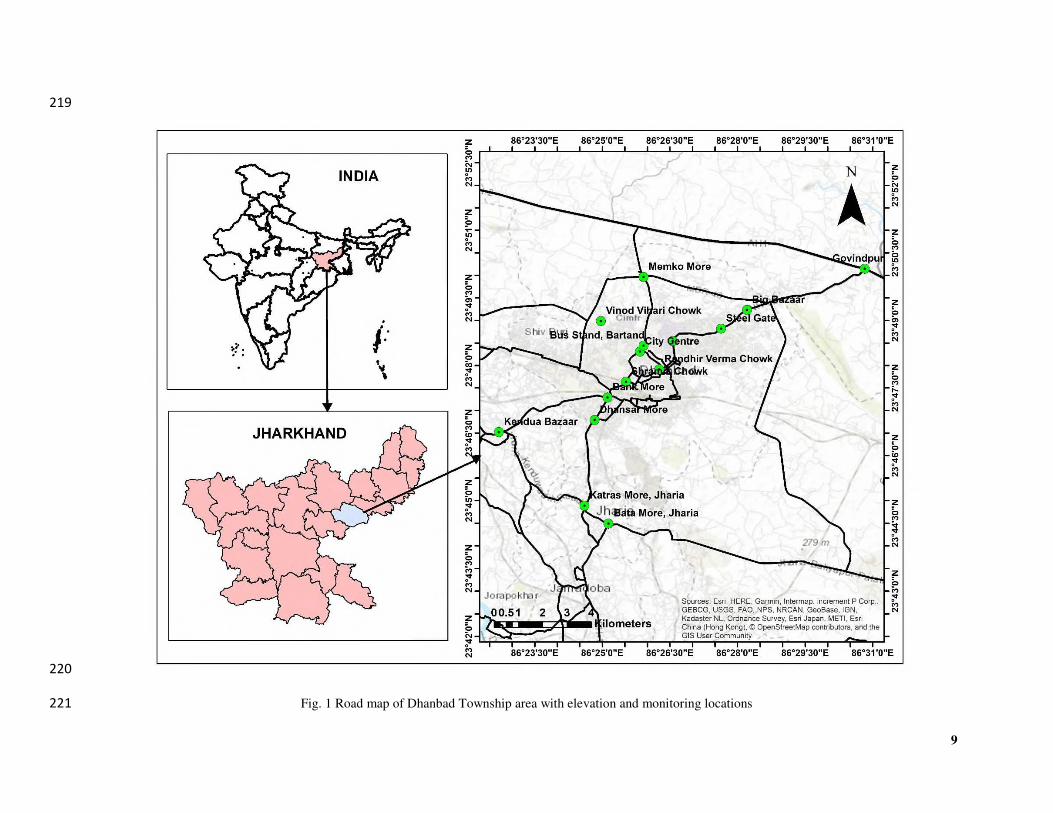
Dhanbad is one of the major coal cities of India. We have selected 15 monitoring points of the Dhanbad city 190
to assess noise pollution and the counting of different types of vehicles in this study. Monitoring points are selected 191
according to major road intersections, junction points, bus stations, markets among the township area, where traffic is 192
always high during peak timing of the day and night hours. Fig. 1 gives the view of road map of Dhanbad township 193
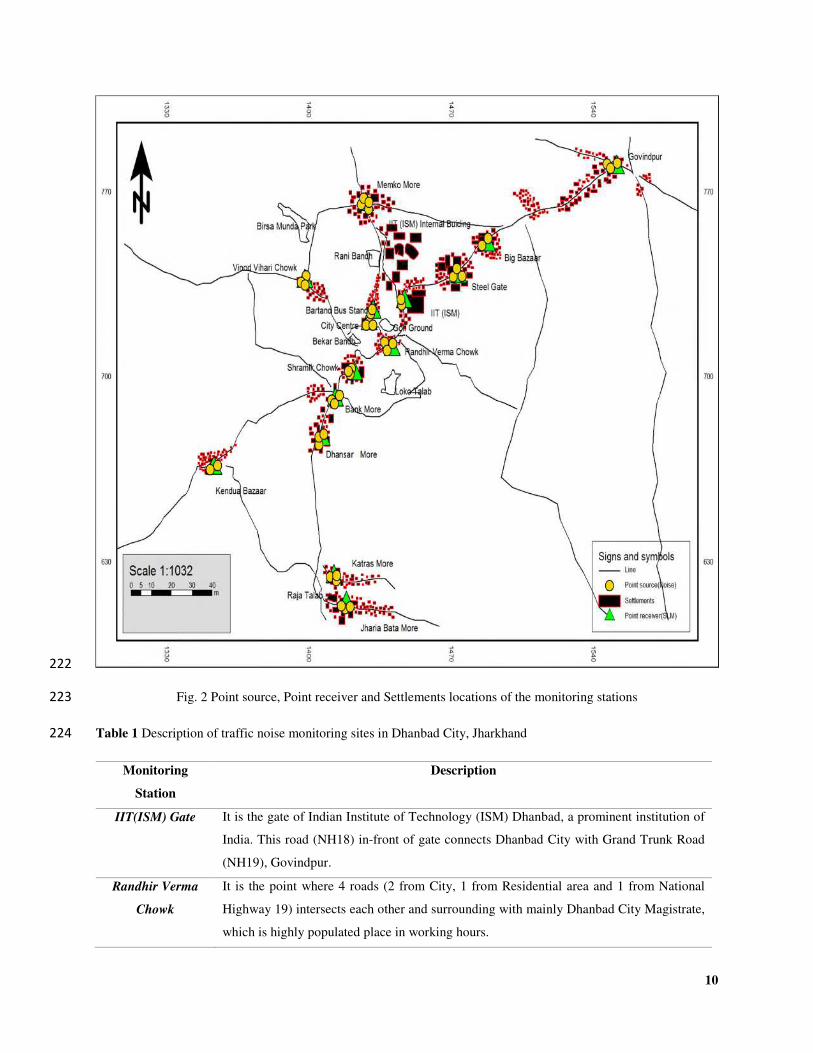
area with monitoring locations. In Fig. 2 shows point source, point receiver and settlements locations of the monitoring 194
stations (Debnath and Singh, 2018).The yellow coding indicates point source, green coding indicates the point receiver 195
and red coding indicates settlements. Noise data collection based on the site selection criteria mentioned in Table 1. 196
197
198
199
200
201
202
203
204
205
206
207
208
209
210
211
212
213
214
215
216
217
218
9
219
220
Fig. 1 Road map of Dhanbad Township area with elevation and monitoring locations221
10
222
Fig. 2 Point source, Point receiver and Settlements locations of the monitoring stations 223
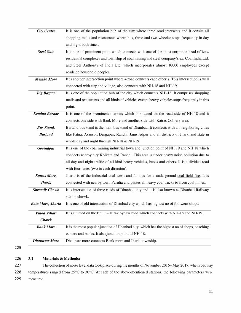
Table 1 Description of traffic noise monitoring sites in Dhanbad City, Jharkhand 224
Monitoring
Station
Description
IIT(ISM) Gate It is the gate of Indian Institute of Technology (ISM) Dhanbad, a prominent institution of
India. This road (NH18) in-front of gate connects Dhanbad City with Grand Trunk Road
(NH19), Govindpur.
Randhir Verma
Chowk
It is the point where 4 roads (2 from City, 1 from Residential area and 1 from National
Highway 19) intersects each other and surrounding with mainly Dhanbad City Magistrate,
which is highly populated place in working hours.
11
City Centre It is one of the population hub of the city where three road intersects and it consist all
shopping malls and restaurants where bus, three and two wheeler stops frequently in day
and night both times.
Steel Gate It is one of prominent point which connects with one of the most corporate head offices,
residential complexes and township of coal mining and steel company’s ex. Coal India Ltd.
and Steel Authority of India Ltd. which incorporates almost 10000 employees except
roadside household peoples.
Memko More It is another intersection point where 4 road connects each other’s. This intersection is well
connected with city and village, also connects with NH-18 and NH-19.
Big Bazaar It is one of the population hub of the city which connects NH -18. It comprises shopping
malls and restaurants and all kinds of vehicles except heavy vehicles stops frequently in this
point.
Kendua Bazaar It is one of the prominent markets which is situated on the road side of NH-18 and it
connects one side with Bank More and another side with Katras Colliery area.
Bus Stand,
Bartand
Bartand bus stand is the main bus stand of Dhanbad. It connects with all neighboring cities
like Patna, Asansol, Durgapur, Ranchi, Jamshedpur and all districts of Jharkhand state in
whole day and night through NH-18 & NH-19.
Govindpur It is one of the coal mining industrial town and junction point of NH 19 and NH 18 which
connects nearby city Kolkata and Ranchi. This area is under heavy noise pollution due to
all day and night traffic of all kind heavy vehicles, buses and others. It is a divided road
with four lanes (two in each direction).
Katras More,
Jharia
Jharia is of the industrial coal town and famous for a underground coal field fire. It is
connected with nearby town Purulia and passes all heavy coal trucks to from coal mines.
Shramik Chowk It is intersection of three roads of Dhanbad city and it is also known as Dhanbad Railway
station chowk.
Bata More, Jharia It is one of old intersection of Dhanbad city which has highest no of footwear shops.
Vinod Vihari
Chowk
It is situated on the Bhuli – Hirak bypass road which connects with NH-18 and NH-19.
Bank More It is the most popular junction of Dhanbad city, which has the highest no of shops, coaching
centers and banks. It also junction point of NH-18.
Dhaunsar More Dhaunsar more connects Bank more and Jharia township.
225
3.1 Materials & Methods: 226
The collection of noise level data took place during the months of November 2016– May 2017, when roadway 227
temperatures ranged from 25°C to 30°C. At each of the above-mentioned stations, the following parameters were 228
measured: 229
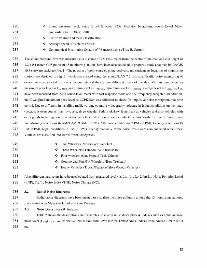
12
Sound pressure level, using Bruel & Kjaer 2238 Mediator Integrating Sound Level Meter 230
(According to IS: 3028:1998) 231
Traffic volume and their Classification 232
Average speed of vehicles (Km/h) 233
Geographical Positioning System (GPS meter) using eTrex H, Garmin 234
The sound pressure level was measured at a distance of 7.5 ± 0.2 meter from the centre of the road and at a height of 235
1.2 ± 0.1 meter. GPS points of 15 monitoring stations have been also collected to prepare a study area map by ArcGIS 236
10.3 software package (Fig. 1). The position of point sources, point receivers, and settlements locations of monitoring 237
stations are depicted in Fig. 2, which was created using the SoundPLAN 7.2 software. Traffic noise monitoring of 238
every points conducted for every 3-hour interval during five different times of the day. Various parameters as 239
maximum peak level as LAFMaxP, maximum level as LAFMaxL, minimum level as LAFMinL, average level as LAeq, L10, L90, 240
have been recorded from 2238 sound level meter with fast response mode and “A” frequency weighted. In addition, 241
the C weighted maximum peak level as LCPKMax was collected to check for impulsive noise throughout that time 242
period. Due to difficulty in installing traffic volume counting videography software in Indian conditions on the roads 243
(because it even counts man, by-cycle, three wheeler Pedal rickshaw & animals as vehicles and also vehicles with 244
extra goods looks big counts as heavy vehicles), traffic counts were conducted continuously for five different times 245
viz. Morning conditions (6 AM-9 AM, 9 AM- 12 PM), Afternoon conditions( 2 PM – 5 PM), Evening conditions (5 246
PM- 8 PM), Night conditions (8 PM- 11 PM) in a day manually while noise levels were also collected same times. 247
Vehicles are classified into five different categories. 248
Two Wheelers (Motor cycle, scooter) 249
Three Wheelers (Tempoo, Auto Rickshaw) 250
Four wheelers (Car, Prepaid Taxi, Others) 251
Commercial Four/Six Wheelers (Bus/ Trekkars) 252
Heavy Vehicles (Trucks/Tractors/Tilors /Goods Vehicles) 253
Also, different parameters have been calculated from measured level viz. LAeq, L10, L90, 24hrs Ldn, Noise Pollution Level 254
(LNP), Traffic Noise Index (TNI), Noise Climate (NC). 255
3.2 Radial Noise Diagrams 256
Radial noise diagrams have been created to visualize the noise pollution among the 15 monitoring stations. 257
It is created with Microsoft Excel Software Package. 258
3.3 Noise Descriptors & Indexes 259
Table 2 shows the descriptions and principles of several noise descriptors & indexes such as 15hrs average 260
noise level (LAeq), L10 , L90 , 24hrs Ldn , Noise Pollution Level (LNP), Traffic Noise Index (TNI), Noise Climate (NC) 261
etc. 262
13
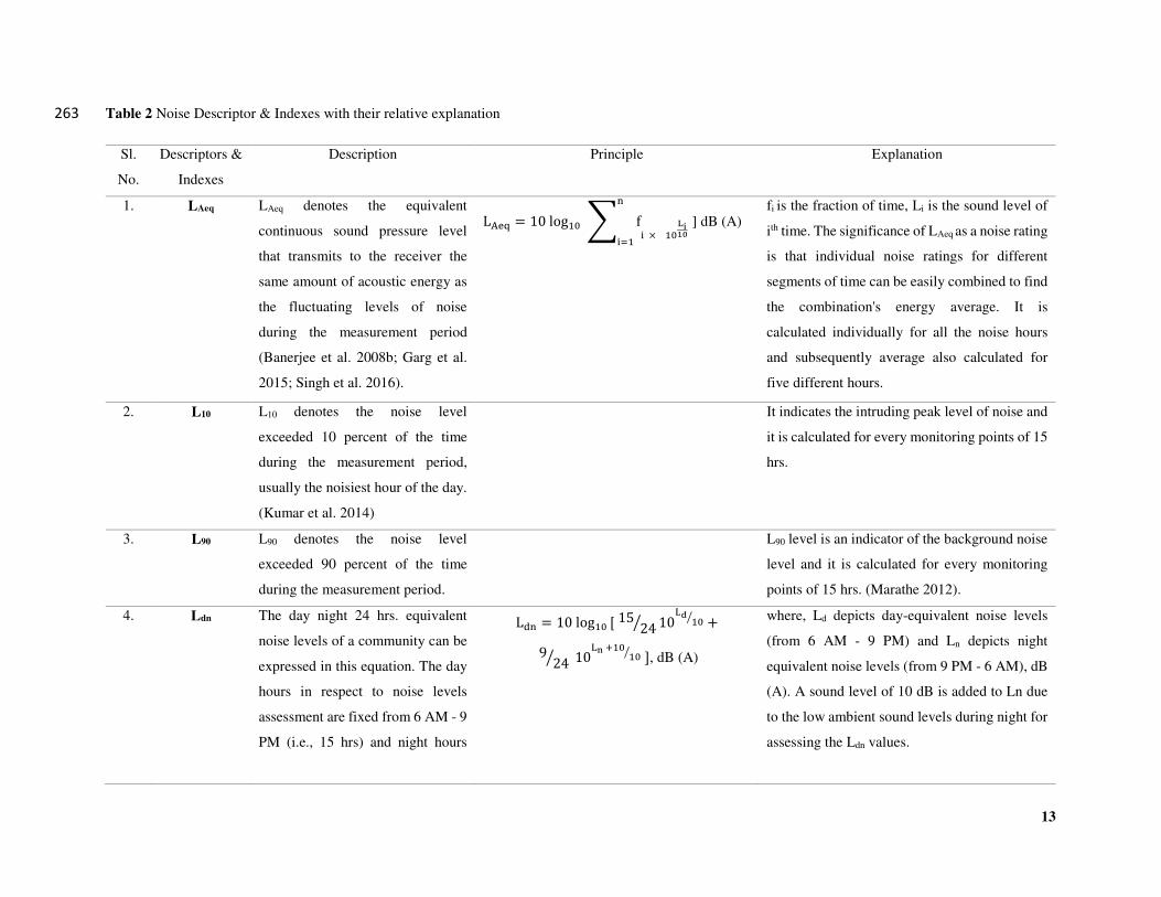
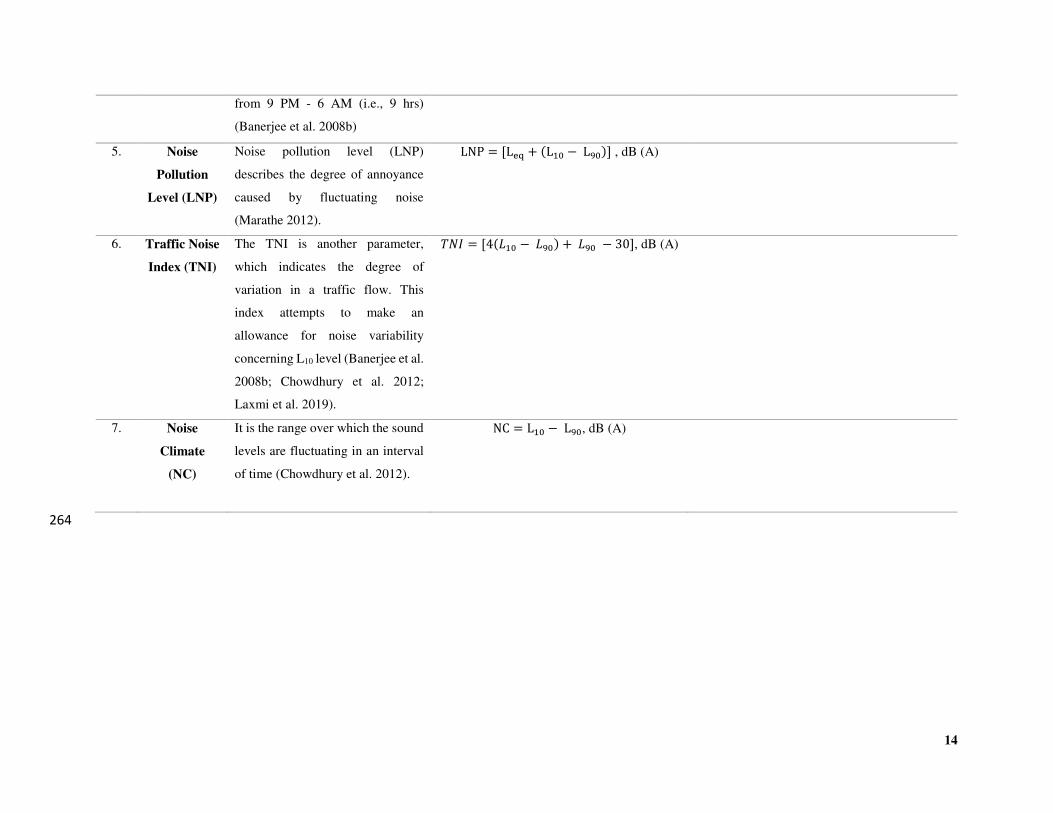
Table 2 Noise Descriptor & Indexes with their relative explanation 263
Sl.
No.
Descriptors &
Indexes
Description Principle Explanation
1. LAeq LAeq denotes the equivalent
continuous sound pressure level
that transmits to the receiver the
same amount of acoustic energy as
the fluctuating levels of noise
during the measurement period
(Banerjee et al. 2008b; Garg et al.
2015; Singh et al. 2016).
LAeq = 10 log10 ∑ fi × 10Li10ni=1 ] dB (A)
fi is the fraction of time, Li is the sound level of
ith time. The significance of LAeq as a noise rating
is that individual noise ratings for different
segments of time can be easily combined to find
the combination's energy average. It is
calculated individually for all the noise hours
and subsequently average also calculated for
five different hours.
2. L10 L10 denotes the noise level
exceeded 10 percent of the time
during the measurement period,
usually the noisiest hour of the day.
(Kumar et al. 2014)
It indicates the intruding peak level of noise and
it is calculated for every monitoring points of 15
hrs.
3. L90 L90 denotes the noise level
exceeded 90 percent of the time
during the measurement period.
L90 level is an indicator of the background noise
level and it is calculated for every monitoring
points of 15 hrs. (Marathe 2012).
4. Ldn The day night 24 hrs. equivalent
noise levels of a community can be
expressed in this equation. The day
hours in respect to noise levels
assessment are fixed from 6 AM - 9
PM (i.e., 15 hrs) and night hours
Ldn = 10 log10 [ 1524⁄ 10
Ld 10⁄ +
924⁄ 10
Ln +10 10⁄ ], dB (A)
where, Ld depicts day-equivalent noise levels
(from 6 AM - 9 PM) and Ln depicts night
equivalent noise levels (from 9 PM - 6 AM), dB
(A). A sound level of 10 dB is added to Ln due
to the low ambient sound levels during night for
assessing the Ldn values.
14
from 9 PM - 6 AM (i.e., 9 hrs)
(Banerjee et al. 2008b)
5. Noise
Pollution
Level (LNP)
Noise pollution level (LNP)
describes the degree of annoyance
caused by fluctuating noise
(Marathe 2012).
LNP = [Leq + (L10 − L90)] , dB (A)
6. Traffic Noise
Index (TNI)
The TNI is another parameter,
which indicates the degree of
variation in a traffic flow. This
index attempts to make an
allowance for noise variability
concerning L10 level (Banerjee et al.
2008b; Chowdhury et al. 2012;
Laxmi et al. 2019).
𝑇𝑁𝐼 = [4(𝐿10 − 𝐿90) + 𝐿90 − 30], dB (A)
7. Noise
Climate
(NC)
It is the range over which the sound
levels are fluctuating in an interval
of time (Chowdhury et al. 2012).
NC = L10 − L90, dB (A)
264
15
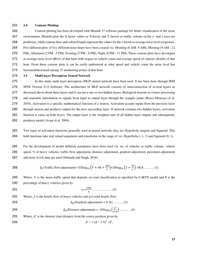
3.4 Contour Plotting265
Contour plotting has been developed with Minitab 17 software package for better visualization of the noise 266
environment. Minitab plots the X factor values as Velocity and Y factors as traffic volume on the x- and y-axes are 267
predictors, while contour lines and colored bands represent the values for the z-factor as average noise level (response). 268
Five different plots of five different noise hours have been created viz. Morning (6 AM- 9 AM), Morning (9 AM - 12 269
PM), Afternoon (2 PM - 5 PM), Evening (5 PM - 8 PM), Night (8 PM - 11 PM). These contour plots have developed 270
as average noise level dB(A) of that hour with respect to vehicle count and average speed of vehicles (Km/h) of that 271
hour. From these contour plots it can be easily understood at what speed and vehicle count the noise level has 272
increased/decreased among 15 monitoring points of that hour. 273
3.5 Multi-layer Perceptron Neural Network274
In this study multi-layer perceptron (MLP) neural network have been used. It has been done through IBM 275
SPSS Version 21.0 Software. The architecture of MLP network consists of interconnection of several layers as 276
discussed above about three layers and it can have one or two hidden layers. Biological neurons as a basic processing 277
unit transmits information or signals from input to output layer through the synaptic joints (Bravo-Moncayo et al. 278
2019). Activation is a specific mathematical function of a neuron. Activation accepts inputs from the previous layer 279
through neuron and produces output for the next succeeding layer. If network contains two hidden layers, activation 280
function is same on both layers. The output layer is the weighted sum of all hidden layer outputs and subsequently 281
produces model (Avşar et al. 2004). 282
Two types of activation functions generally used in neural network; they are Hyperbolic tangent and Sigmoid. This 283
both functions take real valued arguments and transforms in the range of viz. Hyperbolic (–1, 1) and Sigmoid (0, 1). 284
For the development of model different parameters have been used viz. no. of vehicles as traffic volume, vehicle 285
speed, % of heavy vehicles, traffic flow adjustment, distance adjustment, gradient adjustment, pavement adjustment 286
and noise levels data are used (Debnath and Singh, 2018). 287
∆𝑓(Traffic flow adjustment) =33𝑙𝑜𝑔10 (𝑉 + 40 +500𝑉 )+10𝑙𝑜𝑔10 (1 +
5𝑃𝑉 )- 68.8………. (1) 288
Where, V is the mean traffic speed that depends on road classification as specified by CoRTN model and P is the 289
percentage of heavy vehicles given by 290
p =100𝑓𝑞 ……………… (2) 291
Where, 𝑓 is the hourly flow of heavy vehicles and q is total hourly flow. 292 ∆𝑔(Gradient adjustment) = 0.3G………. (3) 293 ∆𝑑(Distance adjustment) = -10𝑙𝑜𝑔10 ( 𝑑′13.5) ………. (4) 294
Where, 𝑑′ is the shortest slant distance from the source position given by 295 𝑑′ = √ (d + 3.5)2 +ℎ2, 296
16
d is the shortest horizontal distance between the nearside carriageway edge and the reception point, and ℎ is the vertical 297
distance between the source position and the reception point. 298 ∆𝑝(Pavement type adjustment) = 4 − 0.03𝑃 ………. (5) 299
Where, P is the percentage of heavy vehicles. 300
The data was processed using IBM SPSS Version 21.0 Package. LAeq observed as output parameters. In comparison 301
to prior researches, this is a huge sample size that would allow for the development of a generally recognized ANN 302
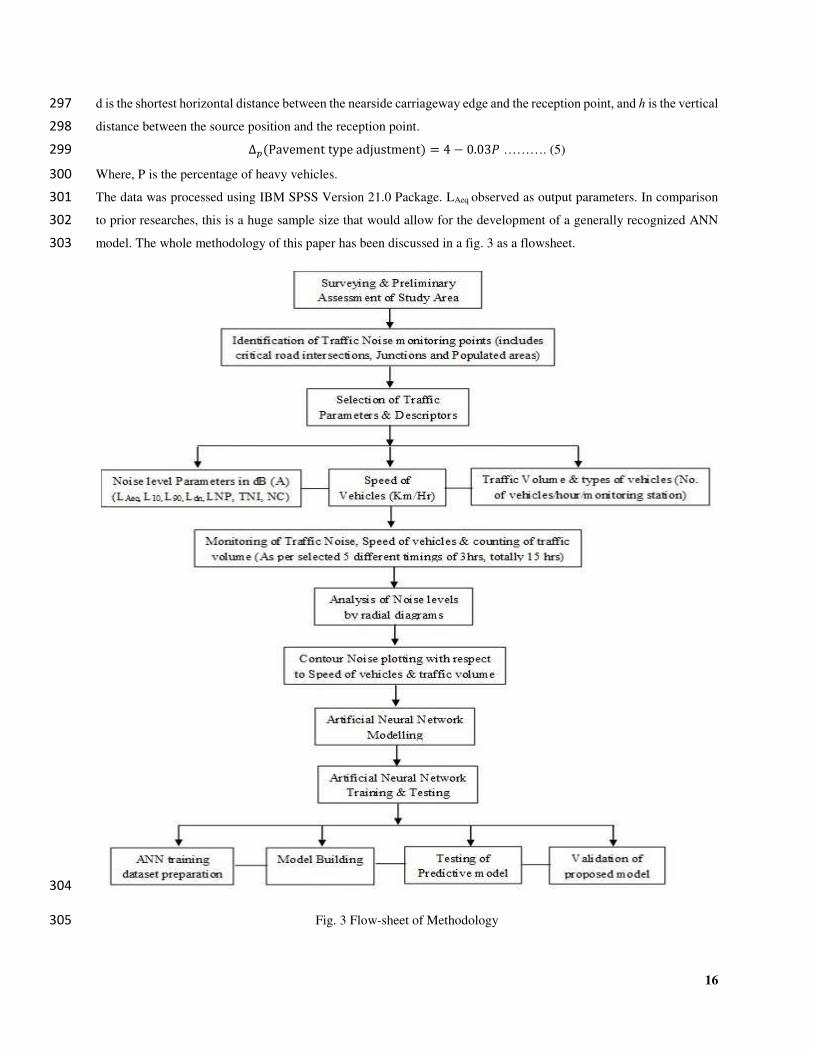
model. The whole methodology of this paper has been discussed in a fig. 3 as a flowsheet. 303
304
Fig. 3 Flow-sheet of Methodology 305
17
4.1 Results & Discussions 306
4.1.1 Noise level analysis 307
Noise level recorded from Sound Level Meter have been analyzed according to peak and non-peak hours of 308
five different timings viz. 309
Non-Peak morning hours (6 AM – 9 AM) 310
Peak morning hours (9 AM – 12 PM) 311
Non-Peak Afternoon hours (2 PM – 5 PM) 312
Peak Evening hours (5 PM – 8 PM) 313
Non-Peak Night hours (8 PM – 11 PM) 314
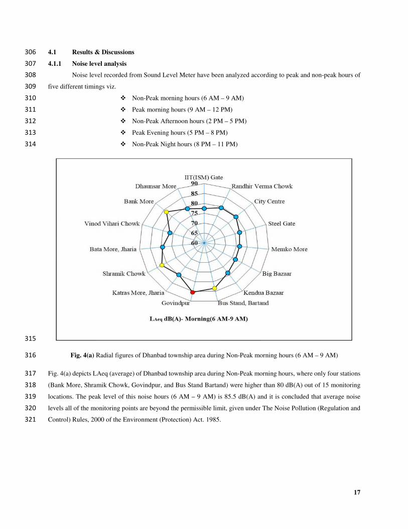
315
Fig. 4(a) Radial figures of Dhanbad township area during Non-Peak morning hours (6 AM – 9 AM) 316
Fig. 4(a) depicts LAeq (average) of Dhanbad township area during Non-Peak morning hours, where only four stations 317
(Bank More, Shramik Chowk, Govindpur, and Bus Stand Bartand) were higher than 80 dB(A) out of 15 monitoring 318
locations. The peak level of this noise hours (6 AM – 9 AM) is 85.5 dB(A) and it is concluded that average noise 319
levels all of the monitoring points are beyond the permissible limit, given under The Noise Pollution (Regulation and 320
Control) Rules, 2000 of the Environment (Protection) Act. 1985. 321
18
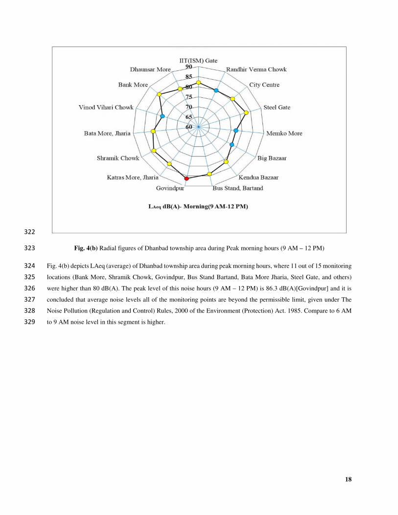
322
Fig. 4(b) Radial figures of Dhanbad township area during Peak morning hours (9 AM – 12 PM) 323
Fig. 4(b) depicts LAeq (average) of Dhanbad township area during peak morning hours, where 11 out of 15 monitoring 324
locations (Bank More, Shramik Chowk, Govindpur, Bus Stand Bartand, Bata More Jharia, Steel Gate, and others) 325
were higher than 80 dB(A). The peak level of this noise hours (9 AM – 12 PM) is 86.3 dB(A)[Govindpur] and it is 326
concluded that average noise levels all of the monitoring points are beyond the permissible limit, given under The 327
Noise Pollution (Regulation and Control) Rules, 2000 of the Environment (Protection) Act. 1985. Compare to 6 AM 328
to 9 AM noise level in this segment is higher. 329
19
330
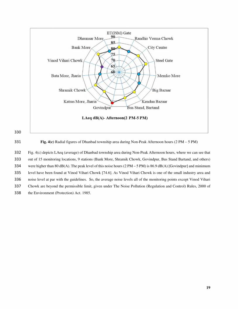
Fig. 4(c) Radial figures of Dhanbad township area during Non-Peak Afternoon hours (2 PM – 5 PM) 331
Fig. 4(c) depicts LAeq (average) of Dhanbad township area during Non-Peak Afternoon hours, where we can see that 332
out of 15 monitoring locations, 9 stations (Bank More, Shramik Chowk, Govindpur, Bus Stand Bartand, and others) 333
were higher than 80 dB(A). The peak level of this noise hours (2 PM – 5 PM) is 86.9 dB(A) [Govindpur] and minimum 334
level have been found at Vinod Vihari Chowk [74.6]. As Vinod Vihari Chowk is one of the small industry area and 335
noise level at par with the guidelines. So, the average noise levels all of the monitoring points except Vinod Vihari 336
Chowk are beyond the permissible limit, given under The Noise Pollution (Regulation and Control) Rules, 2000 of 337
the Environment (Protection) Act. 1985. 338
20
339
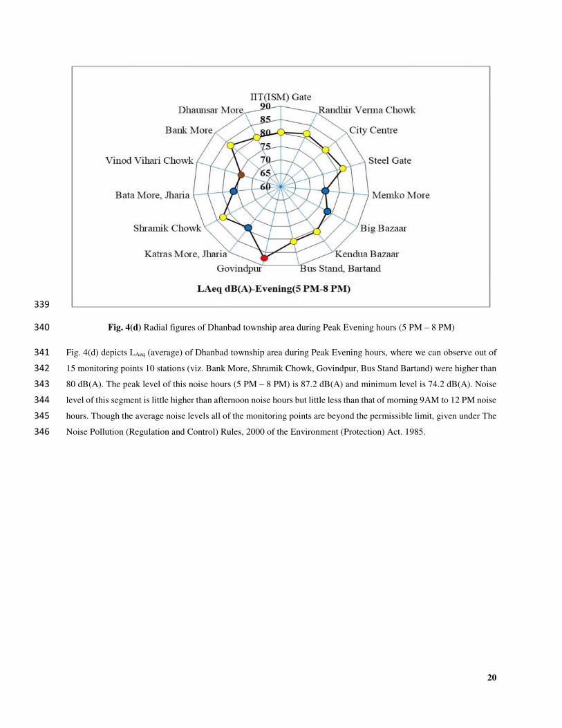
Fig. 4(d) Radial figures of Dhanbad township area during Peak Evening hours (5 PM – 8 PM) 340
Fig. 4(d) depicts LAeq (average) of Dhanbad township area during Peak Evening hours, where we can observe out of 341
15 monitoring points 10 stations (viz. Bank More, Shramik Chowk, Govindpur, Bus Stand Bartand) were higher than 342
80 dB(A). The peak level of this noise hours (5 PM – 8 PM) is 87.2 dB(A) and minimum level is 74.2 dB(A). Noise 343
level of this segment is little higher than afternoon noise hours but little less than that of morning 9AM to 12 PM noise 344
hours. Though the average noise levels all of the monitoring points are beyond the permissible limit, given under The 345
Noise Pollution (Regulation and Control) Rules, 2000 of the Environment (Protection) Act. 1985. 346
21
347
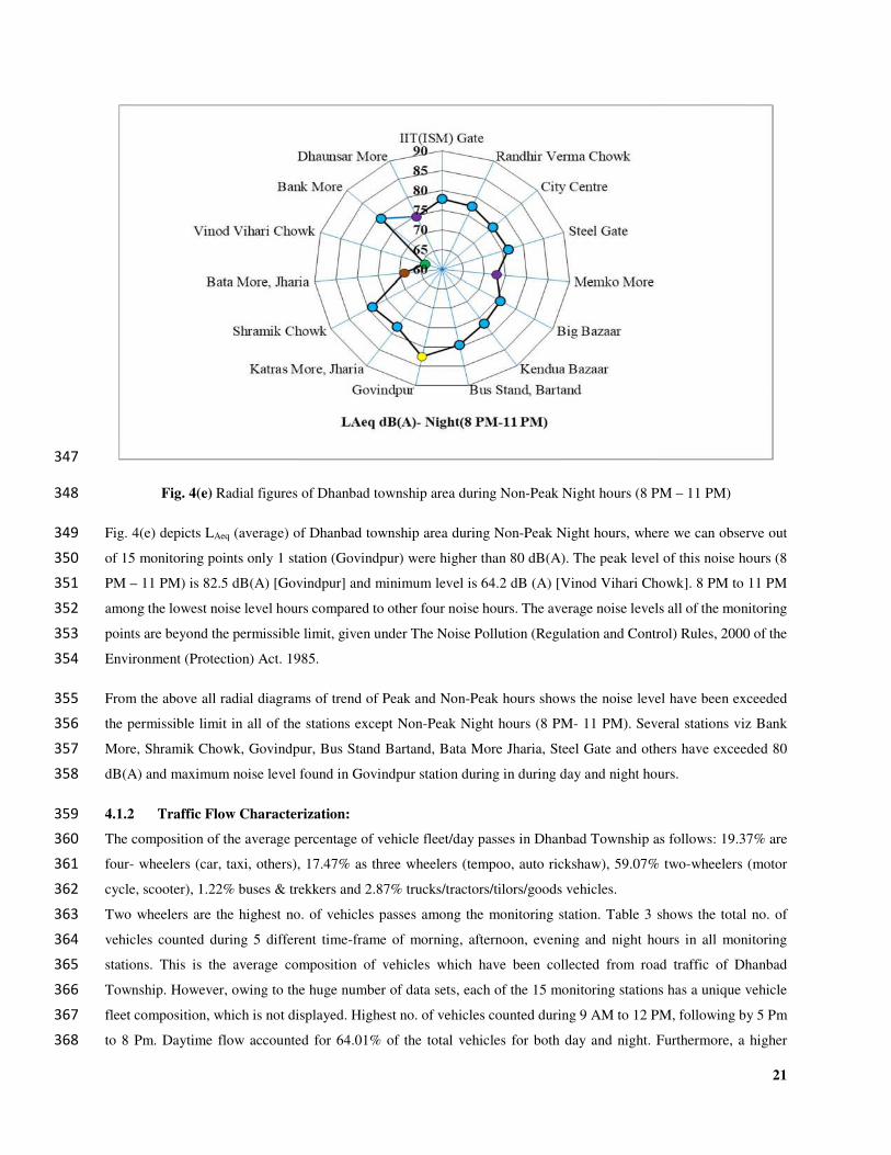
Fig. 4(e) Radial figures of Dhanbad township area during Non-Peak Night hours (8 PM – 11 PM) 348
Fig. 4(e) depicts LAeq (average) of Dhanbad township area during Non-Peak Night hours, where we can observe out 349
of 15 monitoring points only 1 station (Govindpur) were higher than 80 dB(A). The peak level of this noise hours (8 350
PM – 11 PM) is 82.5 dB(A) [Govindpur] and minimum level is 64.2 dB (A) [Vinod Vihari Chowk]. 8 PM to 11 PM 351
among the lowest noise level hours compared to other four noise hours. The average noise levels all of the monitoring 352
points are beyond the permissible limit, given under The Noise Pollution (Regulation and Control) Rules, 2000 of the 353
Environment (Protection) Act. 1985. 354
From the above all radial diagrams of trend of Peak and Non-Peak hours shows the noise level have been exceeded 355
the permissible limit in all of the stations except Non-Peak Night hours (8 PM- 11 PM). Several stations viz Bank 356
More, Shramik Chowk, Govindpur, Bus Stand Bartand, Bata More Jharia, Steel Gate and others have exceeded 80 357
dB(A) and maximum noise level found in Govindpur station during in during day and night hours. 358
4.1.2 Traffic Flow Characterization: 359
The composition of the average percentage of vehicle fleet/day passes in Dhanbad Township as follows: 19.37% are 360
four- wheelers (car, taxi, others), 17.47% as three wheelers (tempoo, auto rickshaw), 59.07% two-wheelers (motor 361
cycle, scooter), 1.22% buses & trekkers and 2.87% trucks/tractors/tilors/goods vehicles. 362
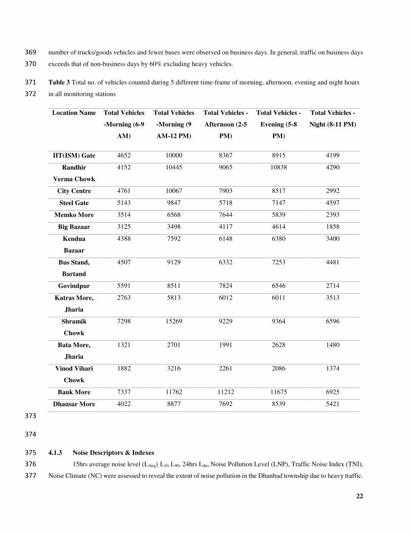
Two wheelers are the highest no. of vehicles passes among the monitoring station. Table 3 shows the total no. of 363
vehicles counted during 5 different time-frame of morning, afternoon, evening and night hours in all monitoring 364
stations. This is the average composition of vehicles which have been collected from road traffic of Dhanbad 365
Township. However, owing to the huge number of data sets, each of the 15 monitoring stations has a unique vehicle 366
fleet composition, which is not displayed. Highest no. of vehicles counted during 9 AM to 12 PM, following by 5 Pm 367
to 8 Pm. Daytime flow accounted for 64.01% of the total vehicles for both day and night. Furthermore, a higher 368
22
number of trucks/goods vehicles and fewer buses were observed on business days. In general, traffic on business days 369
exceeds that of non-business days by 60% excluding heavy vehicles. 370
Table 3 Total no. of vehicles counted during 5 different time-frame of morning, afternoon, evening and night hours 371
in all monitoring stations 372
Location Name Total Vehicles
-Morning (6-9
AM)
Total Vehicles
-Morning (9
AM-12 PM)
Total Vehicles -
Afternoon (2-5
PM)
Total Vehicles -
Evening (5-8
PM)
Total Vehicles -
Night (8-11 PM)
IIT(ISM) Gate 4652 10000 8367 8915 4199
Randhir
Verma Chowk
4152 10445 9065 10838 4290
City Centre 4761 10067 7903 8517 2992
Steel Gate 5143 9847 5718 7147 4597
Memko More 3514 6568 7644 5839 2393
Big Bazaar 3125 3498 4117 4614 1858
Kendua
Bazaar
4388 7592 6148 6380 3400
Bus Stand,
Bartand
4507 9129 6332 7253 4481
Govindpur 5591 8511 7824 6546 2714
Katras More,
Jharia
2763 5813 6012 6011 3513
Shramik
Chowk
7298 15269 9229 9364 6596
Bata More,
Jharia
1321 2701 1991 2628 1480
Vinod Vihari
Chowk
1882 3216 2261 2086 1374
Bank More 7337 11762 11212 11675 6925
Dhansar More 4022 8877 7692 8539 5421
373
374
4.1.3 Noise Descriptors & Indexes 375
15hrs average noise level (LAeq), L10, L90, 24hrs Ldn, Noise Pollution Level (LNP), Traffic Noise Index (TNI), 376
Noise Climate (NC) were assessed to reveal the extent of noise pollution in the Dhanbad township due to heavy traffic. 377
23
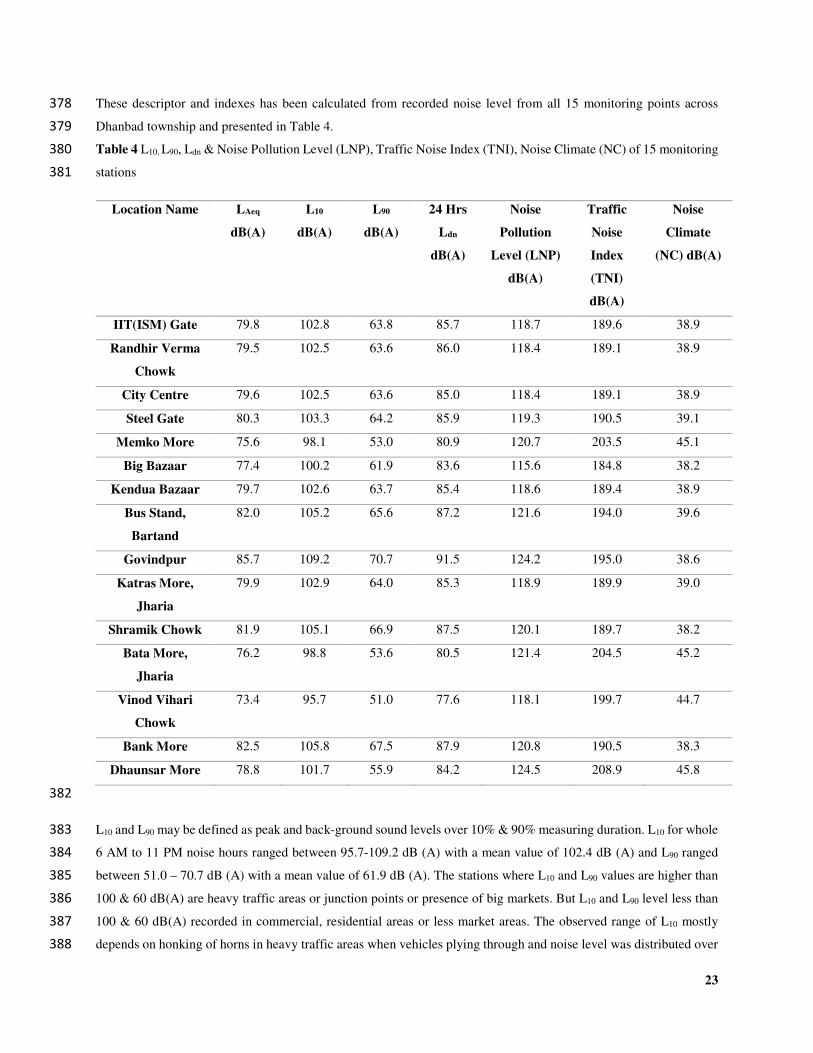
These descriptor and indexes has been calculated from recorded noise level from all 15 monitoring points across 378
Dhanbad township and presented in Table 4. 379
Table 4 L10, L90, Ldn & Noise Pollution Level (LNP), Traffic Noise Index (TNI), Noise Climate (NC) of 15 monitoring 380
stations 381
Location Name LAeq
dB(A)
L10
dB(A)
L90
dB(A)
24 Hrs
Ldn
dB(A)
Noise
Pollution
Level (LNP)
dB(A)
Traffic
Noise
Index
(TNI)
dB(A)
Noise
Climate
(NC) dB(A)
IIT(ISM) Gate 79.8 102.8 63.8 85.7 118.7 189.6 38.9
Randhir Verma
Chowk
79.5 102.5 63.6 86.0 118.4 189.1 38.9
City Centre 79.6 102.5 63.6 85.0 118.4 189.1 38.9
Steel Gate 80.3 103.3 64.2 85.9 119.3 190.5 39.1
Memko More 75.6 98.1 53.0 80.9 120.7 203.5 45.1
Big Bazaar 77.4 100.2 61.9 83.6 115.6 184.8 38.2
Kendua Bazaar 79.7 102.6 63.7 85.4 118.6 189.4 38.9
Bus Stand,
Bartand
82.0 105.2 65.6 87.2 121.6 194.0 39.6
Govindpur 85.7 109.2 70.7 91.5 124.2 195.0 38.6
Katras More,
Jharia
79.9 102.9 64.0 85.3 118.9 189.9 39.0
Shramik Chowk 81.9 105.1 66.9 87.5 120.1 189.7 38.2
Bata More,
Jharia
76.2 98.8 53.6 80.5 121.4 204.5 45.2
Vinod Vihari
Chowk
73.4 95.7 51.0 77.6 118.1 199.7 44.7
Bank More 82.5 105.8 67.5 87.9 120.8 190.5 38.3
Dhaunsar More 78.8 101.7 55.9 84.2 124.5 208.9 45.8
382
L10 and L90 may be defined as peak and back-ground sound levels over 10% & 90% measuring duration. L10 for whole 383
6 AM to 11 PM noise hours ranged between 95.7-109.2 dB (A) with a mean value of 102.4 dB (A) and L90 ranged 384
between 51.0 – 70.7 dB (A) with a mean value of 61.9 dB (A). The stations where L10 and L90 values are higher than 385
100 & 60 dB(A) are heavy traffic areas or junction points or presence of big markets. But L10 and L90 level less than 386
100 & 60 dB(A) recorded in commercial, residential areas or less market areas. The observed range of L10 mostly 387
depends on honking of horns in heavy traffic areas when vehicles plying through and noise level was distributed over 388
24
the time homogenously. But whereas L90 distributed heterogeneously and mostly depends on hourly traffic volume 389
passing through the road. Due to higher L90 as background noise level becomes higher, people living in that area feels 390
annoyance which could lead to health effects. It has been observed from the Table 4 that as L10 and L90 becomes lower 391
results higher TNC, LNP, NC values. 392
Ldn for 24 hrs (including 15 hrs in day time and 9 hrs in night time) ranges from 77.6 to 91.5 dB(A) with a mean value 393
of 84.9 dB(A). Ldn is better descriptor of noise which has been calculated for all stations. Except 2 stations maximum 394
station are fall in higher Ldn range. Lower Ldn value depicts the area is under vegetation (forests, gardens) which act 395
as a noise attenuator. 396
397
398
399
400
401
402
403
404
405
406
407
408
25
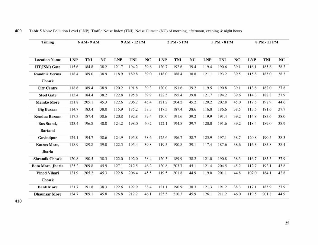
Table 5 Noise Pollution Level (LNP), Traffic Noise Index (TNI), Noise Climate (NC) of morning, afternoon, evening & night hours 409
Timing 6 AM- 9 AM 9 AM - 12 PM 2 PM- 5 PM 5 PM - 8 PM 8 PM- 11 PM
Location Name LNP TNI NC LNP TNI NC LNP TNI NC LNP TNI NC LNP TNI NC
IIT(ISM) Gate 115.6 184.8 38.2 121.7 194.2 39.6 120.7 192.6 39.4 119.4 190.6 39.1 116.1 185.6 38.3
Randhir Verma
Chowk
118.4 189.0 38.9 118.9 189.8 39.0 118.0 188.4 38.8 121.1 193.2 39.5 115.8 185.0 38.3
City Centre 118.6 189.4 38.9 120.2 191.8 39.3 120.0 191.6 39.2 119.5 190.8 39.1 113.8 182.0 37.8
Steel Gate 115.4 184.4 38.2 122.8 195.8 39.9 122.5 195.4 39.8 121.7 194.2 39.6 114.3 182.8 37.9
Memko More 121.8 205.1 45.3 122.6 206.2 45.4 121.2 204.2 45.2 120.2 202.8 45.0 117.5 198.9 44.6
Big Bazaar 114.7 183.4 38.0 115.9 185.2 38.3 117.3 187.4 38.6 116.8 186.6 38.5 113.5 181.6 37.7
Kendua Bazaar 117.3 187.4 38.6 120.8 192.8 39.4 120.0 191.6 39.2 119.9 191.4 39.2 114.8 183.6 38.0
Bus Stand,
Bartand
123.4 196.8 40.0 124.2 198.0 40.2 122.1 194.8 39.7 120.0 191.6 39.2 118.4 189.0 38.9
Govindpur 124.1 194.7 38.6 124.9 195.8 38.6 125.6 196.7 38.7 125.9 197.1 38.7 120.8 190.5 38.3
Katras More,
Jharia
118.9 189.8 39.0 122.5 195.4 39.8 119.5 190.8 39.1 117.4 187.6 38.6 116.3 185.8 38.4
Shramik Chowk 120.8 190.5 38.3 122.0 192.0 38.4 120.3 189.9 38.2 121.0 190.8 38.3 116.7 185.3 37.9
Bata More, Jharia 125.2 209.8 45.9 127.1 212.5 46.2 120.8 203.7 45.1 121.4 204.5 45.2 112.7 192.1 43.8
Vinod Vihari
Chowk
121.9 205.2 45.3 122.8 206.4 45.5 119.5 201.8 44.9 119.0 201.1 44.8 107.0 184.1 42.8
Bank More 121.7 191.8 38.3 122.6 192.9 38.4 121.1 190.9 38.3 121.3 191.2 38.3 117.1 185.9 37.9
Dhaunsar More 124.7 209.1 45.8 126.8 212.2 46.1 125.5 210.3 45.9 126.1 211.2 46.0 119.5 201.8 44.9
410
26
The mean value of noise pollution level (LNP) is 120.0 dB(A), with a range of 115.6 – 124.5 dB(A). As previously 411
stated LNP is the degree of annoyance caused by fluctuating noise (Marathe 2012) and it is calculated as difference 412
between 10% and 90% noise plus the average noise level. The Traffic Noise Index (TNI) measures the degree of 413
variation in a traffic flow with respect to L10, and it varies between 184.8 – 208.9 dB(A) with a mean value of 193.9 414
dB(A). Noise Climate (NC) ranges between 38.2 to 45.8 dB(A) with a mean value of 40.5 dB(A). The TNI and LNP 415
values are significantly higher, ranges from 100 to 200 dB(A) and even exceeding 200 dB(A) in some places. These 416
values clearly indicated that high annoyance level in Dhanbad township. From Table 4 it is observed that if we 417
compared between LAeq & LNP and LAeq & TNI noise levels for all the monitoring locations revealed that TNI & LNP 418
level much more than respective LAeq levels. From Table 4 it is clearly understand that noise levels on any period of 419
the day termed as constant but the presence of single event noise values affects percentile levels and called as TNI or 420
even as up to LNP. LNP, TNI and NC of five different noise hours individually have been shown in Table 5. 421
These descriptors though have limited acoustic effects compared to equivalent noise level but they represent the 422
annoyance and disturbing effects, within the peak levels exceeded over 10%, 90% times of noise events. In case day-423
night exposure, it reflects the diurnal variation across the Dhanbad township by considering day and night hours noise 424
levels. Similar way due to high fluctuation level and variations over flow conditions Noise Pollution Level (LNP), 425
Traffic Noise Index (TNI), Noise Climate (NC) has been taken into consideration to explore the extent of pollution 426
level in roadside areas. Also the Traffic Noise Index (TNI) values helps to explore the distance effect in case of 427
allocation of new lands, land-use zoning of any area for infrastructure purposes, or any requirement of placing of extra 428
insulation or acoustic barriers needed in present roadside buildings. 429
4.1.4 Contour noise plotting 430
Contour noise plots for all peak and non-peak hours under different noise hours have been developed by 431
Minitab 17.0 software package. All the plots have been developed as average noise level dB(A) of that hour with 432
respect to vehicle count and average speed of vehicles (Km/h) of that hour. By analyzing contour plots, it can be easily 433
concluded that at what context noise level of that monitoring points have been increased or decreased. Every contour 434
plot depicted with color colour from Green to Red for better visualization. 435
436
27
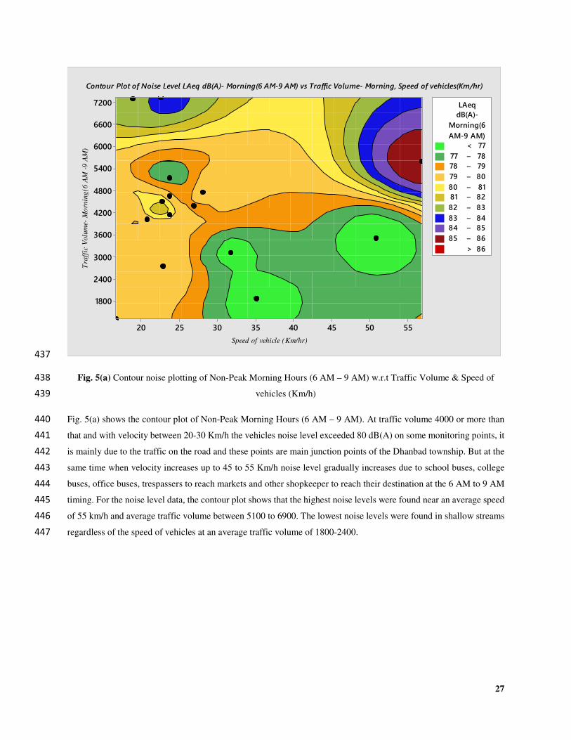
437
Fig. 5(a) Contour noise plotting of Non-Peak Morning Hours (6 AM – 9 AM) w.r.t Traffic Volume & Speed of 438
vehicles (Km/h) 439
Fig. 5(a) shows the contour plot of Non-Peak Morning Hours (6 AM – 9 AM). At traffic volume 4000 or more than 440
that and with velocity between 20-30 Km/h the vehicles noise level exceeded 80 dB(A) on some monitoring points, it 441
is mainly due to the traffic on the road and these points are main junction points of the Dhanbad township. But at the 442
same time when velocity increases up to 45 to 55 Km/h noise level gradually increases due to school buses, college 443
buses, office buses, trespassers to reach markets and other shopkeeper to reach their destination at the 6 AM to 9 AM 444
timing. For the noise level data, the contour plot shows that the highest noise levels were found near an average speed 445
of 55 km/h and average traffic volume between 5100 to 6900. The lowest noise levels were found in shallow streams 446
regardless of the speed of vehicles at an average traffic volume of 1800-2400. 447
Speed of vehicle (Km/hr)
Tra
ffic
Volu
me-
Mo
rnin
g(6
AM
-9A
M)
5550454035302520
7200
6600
6000
5400
4800
4200
3600
3000
2400
1800
>
–
–
–
–
–
–
–
–
–
<
85 86
86
77
77 78
78 79
79 80
80 81
81 82
82 83
83 84
84 85
AM-9 AM)
Morning(6
dB(A)-
LAeq
Contour Plot of Noise Level LAeq dB(A)- Morning(6 AM-9 AM) vs Traffic Volume- Morning, Speed of vehicles(Km/hr)
28
448
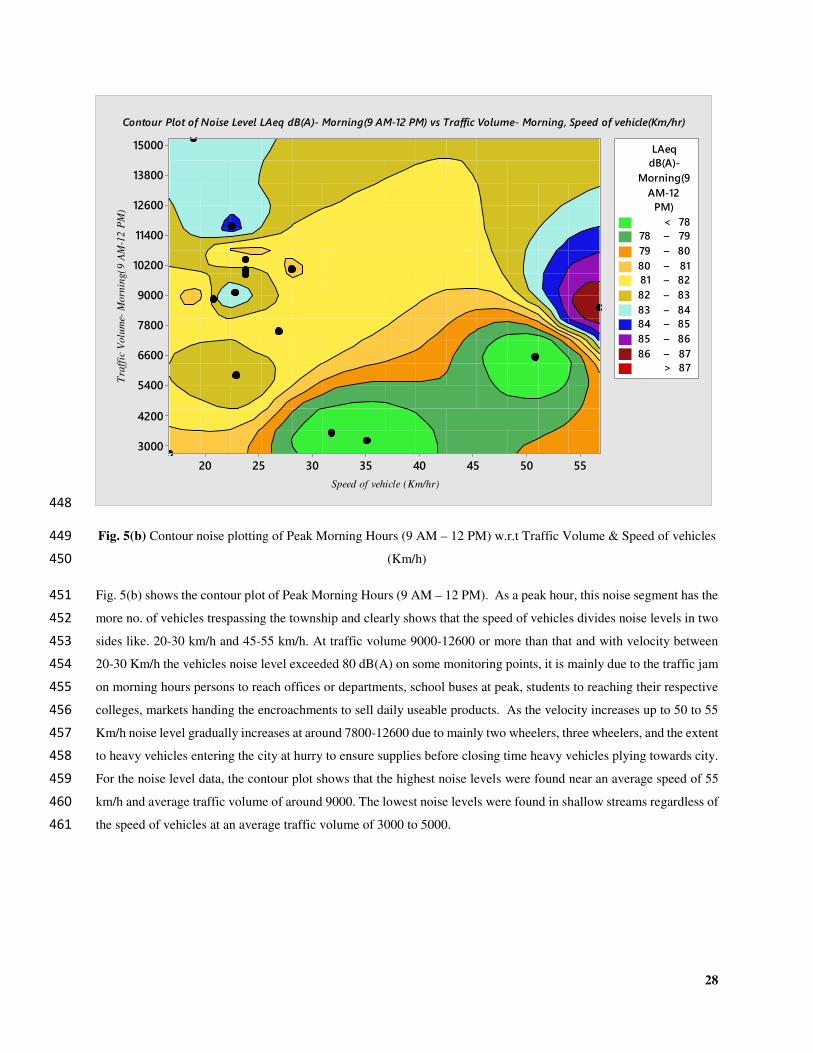
Fig. 5(b) Contour noise plotting of Peak Morning Hours (9 AM – 12 PM) w.r.t Traffic Volume & Speed of vehicles 449
(Km/h) 450
Fig. 5(b) shows the contour plot of Peak Morning Hours (9 AM – 12 PM). As a peak hour, this noise segment has the 451
more no. of vehicles trespassing the township and clearly shows that the speed of vehicles divides noise levels in two 452
sides like. 20-30 km/h and 45-55 km/h. At traffic volume 9000-12600 or more than that and with velocity between 453
20-30 Km/h the vehicles noise level exceeded 80 dB(A) on some monitoring points, it is mainly due to the traffic jam 454
on morning hours persons to reach offices or departments, school buses at peak, students to reaching their respective 455
colleges, markets handing the encroachments to sell daily useable products. As the velocity increases up to 50 to 55 456
Km/h noise level gradually increases at around 7800-12600 due to mainly two wheelers, three wheelers, and the extent 457
to heavy vehicles entering the city at hurry to ensure supplies before closing time heavy vehicles plying towards city. 458
For the noise level data, the contour plot shows that the highest noise levels were found near an average speed of 55 459
km/h and average traffic volume of around 9000. The lowest noise levels were found in shallow streams regardless of 460
the speed of vehicles at an average traffic volume of 3000 to 5000. 461
Speed of vehicle (Km/hr)
Tra
ffic
Volu
me-
Morn
ing(9
AM
-12
PM
)
5550454035302520
15000
13800
12600
11400
10200
9000
7800
6600
5400
4200
3000
>
–
–
–
–
–
–
–
–
–
<
86 87
87
78
78 79
79 80
80 81
81 82
82 83
83 84
84 85
85 86
PM)
AM-12
Morning(9
dB(A)-
LAeq
Contour Plot of Noise Level LAeq dB(A)- Morning(9 AM-12 PM) vs Traffic Volume- Morning, Speed of vehicle(Km/hr)
29
462
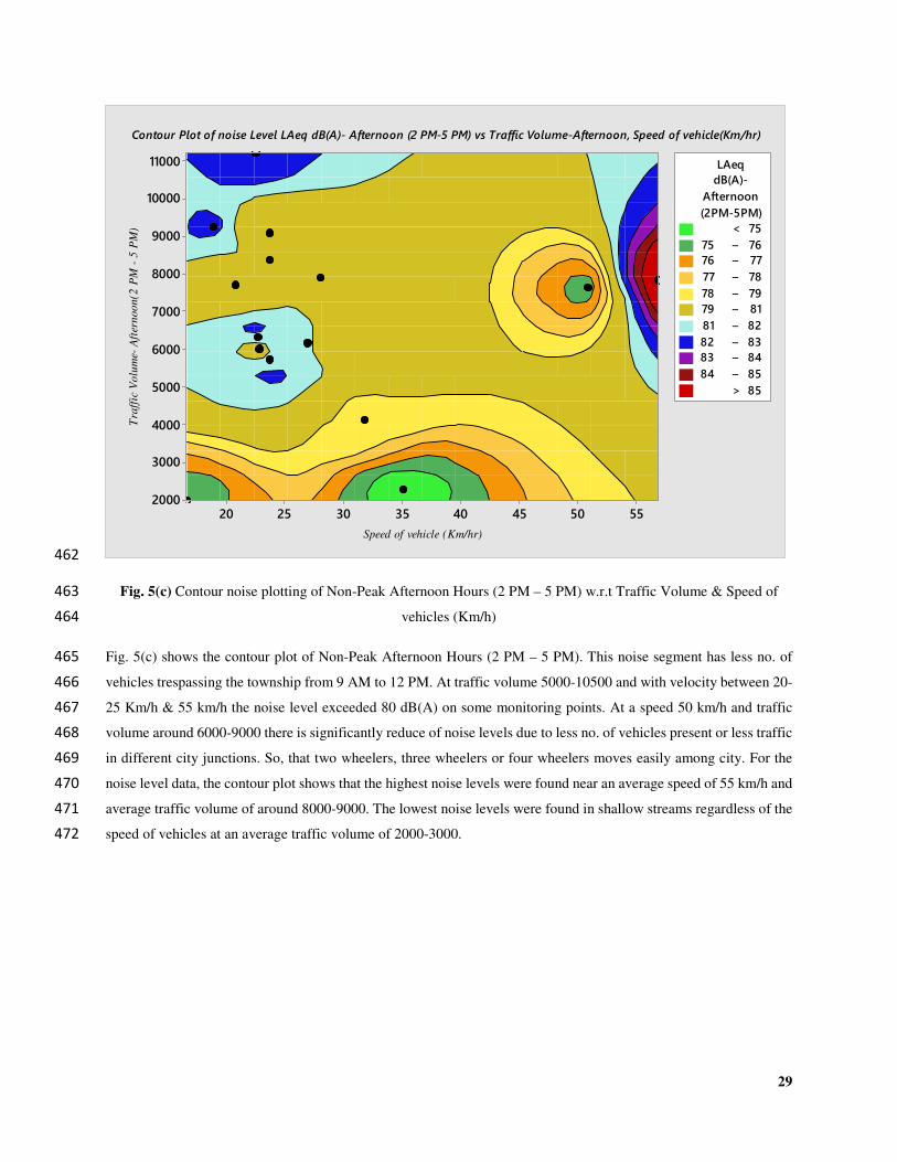
Fig. 5(c) Contour noise plotting of Non-Peak Afternoon Hours (2 PM – 5 PM) w.r.t Traffic Volume & Speed of 463
vehicles (Km/h) 464
Fig. 5(c) shows the contour plot of Non-Peak Afternoon Hours (2 PM – 5 PM). This noise segment has less no. of 465
vehicles trespassing the township from 9 AM to 12 PM. At traffic volume 5000-10500 and with velocity between 20-466
25 Km/h & 55 km/h the noise level exceeded 80 dB(A) on some monitoring points. At a speed 50 km/h and traffic 467
volume around 6000-9000 there is significantly reduce of noise levels due to less no. of vehicles present or less traffic 468
in different city junctions. So, that two wheelers, three wheelers or four wheelers moves easily among city. For the 469
noise level data, the contour plot shows that the highest noise levels were found near an average speed of 55 km/h and 470
average traffic volume of around 8000-9000. The lowest noise levels were found in shallow streams regardless of the 471
speed of vehicles at an average traffic volume of 2000-3000. 472
Speed of vehicle (Km/hr)
Tra
ffic
Vo
lum
e-A
fter
noo
n(2
PM
-5
PM
)
5550454035302520
11000
10000
9000
8000
7000
6000
5000
4000
3000
2000
>
–
–
–
–
–
–
–
–
–
<
84 85
85
75
75 76
76 77
77 78
78 79
79 81
81 82
82 83
83 84
(2PM-5PM)
Afternoon
dB(A)-
LAeq
Contour Plot of noise Level LAeq dB(A)- Afternoon (2 PM-5 PM) vs Traffic Volume-Afternoon, Speed of vehicle(Km/hr)
30
473
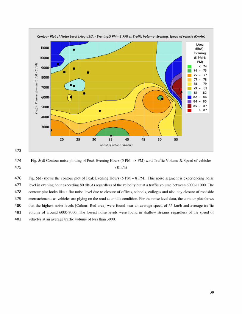
Fig. 5(d) Contour noise plotting of Peak Evening Hours (5 PM – 8 PM) w.r.t Traffic Volume & Speed of vehicles 474
(Km/h) 475
Fig. 5(d) shows the contour plot of Peak Evening Hours (5 PM – 8 PM). This noise segment is experiencing noise 476
level in evening hour exceeding 80 dB(A) regardless of the velocity but at a traffic volume between 6000-11000. The 477
contour plot looks like a flat noise level due to closure of offices, schools, colleges and also day closure of roadside 478
encroachments as vehicles are plying on the road at an idle condition. For the noise level data, the contour plot shows 479
that the highest noise levels [Colour: Red area] were found near an average speed of 55 km/h and average traffic 480
volume of around 6000-7000. The lowest noise levels were found in shallow streams regardless of the speed of 481
vehicles at an average traffic volume of less than 3000. 482
Speed of vehicle (Km/hr)
Tra
ffic
Vo
lum
e-E
ven
ing
(5P
M-
8P
M)
5550454035302520
11000
10000
9000
8000
7000
6000
5000
4000
3000
>
–
–
–
–
–
–
–
–
–
<
85 87
87
74
74 75
75 77
77 78
78 79
79 81
81 82
82 84
84 85
PM)
(5 PM-8
Evening
dB(A)-
LAeq
Contour Plot of Noise Level LAeq dB(A)- Evening(5 PM - 8 PM) vs Traffic Volume- Evening, Speed of vehicle (Km/hr)
31
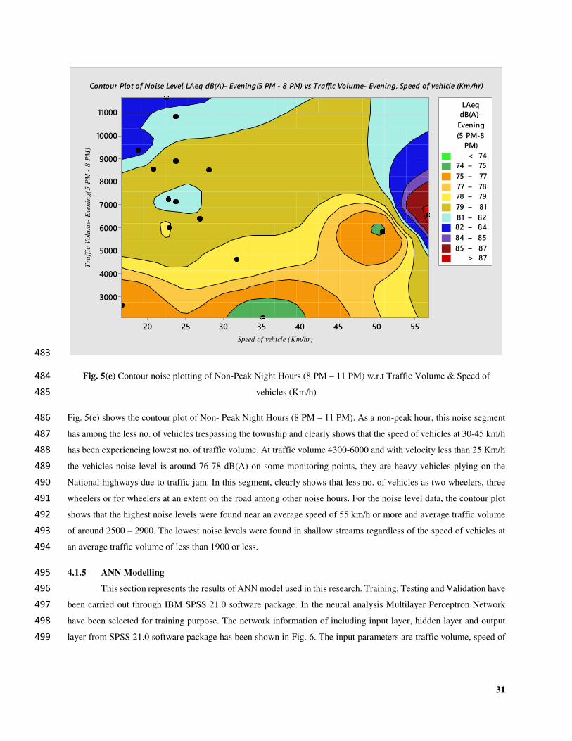
483
Fig. 5(e) Contour noise plotting of Non-Peak Night Hours (8 PM – 11 PM) w.r.t Traffic Volume & Speed of 484
vehicles (Km/h) 485
Fig. 5(e) shows the contour plot of Non- Peak Night Hours (8 PM – 11 PM). As a non-peak hour, this noise segment 486
has among the less no. of vehicles trespassing the township and clearly shows that the speed of vehicles at 30-45 km/h 487
has been experiencing lowest no. of traffic volume. At traffic volume 4300-6000 and with velocity less than 25 Km/h 488
the vehicles noise level is around 76-78 dB(A) on some monitoring points, they are heavy vehicles plying on the 489
National highways due to traffic jam. In this segment, clearly shows that less no. of vehicles as two wheelers, three 490
wheelers or for wheelers at an extent on the road among other noise hours. For the noise level data, the contour plot 491
shows that the highest noise levels were found near an average speed of 55 km/h or more and average traffic volume 492
of around 2500 – 2900. The lowest noise levels were found in shallow streams regardless of the speed of vehicles at 493
an average traffic volume of less than 1900 or less. 494
4.1.5 ANN Modelling 495
This section represents the results of ANN model used in this research. Training, Testing and Validation have 496
been carried out through IBM SPSS 21.0 software package. In the neural analysis Multilayer Perceptron Network 497
have been selected for training purpose. The network information of including input layer, hidden layer and output 498
layer from SPSS 21.0 software package has been shown in Fig. 6. The input parameters are traffic volume, speed of 499
Speed of vehicle (Km/hr)
Tra
ffic
Volu
me-
Eve
nin
g(5
PM
-8
PM
)
5550454035302520
11000
10000
9000
8000
7000
6000
5000
4000
3000
>
–
–
–
–
–
–
–
–
–
<
85 87
87
74
74 75
75 77
77 78
78 79
79 81
81 82
82 84
84 85
PM)
(5 PM-8
Evening
dB(A)-
LAeq
Contour Plot of Noise Level LAeq dB(A)- Evening(5 PM - 8 PM) vs Traffic Volume- Evening, Speed of vehicle (Km/hr)
32
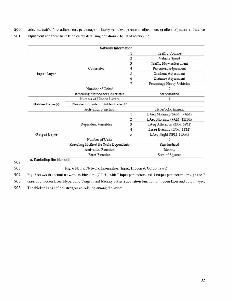
vehicles, traffic flow adjustment, percentage of heavy vehicles, pavement adjustment, gradient adjustment, distance 500
adjustment and these have been calculated using equations 6 to 10 of section 3.5. 501
502
Fig. 6 Neural Network Information (Input, Hidden & Output layer) 503
Fig. 7 shows the neural network architecture (7-7-5), with 7 input parameters and 5 output parameters through the 7 504
units of a hidden layer. Hyperbolic Tangent and Identity act as a activation function of hidden layer and output layer. 505
The thicker lines defines stronger co-relation among the layers. 506
33
507
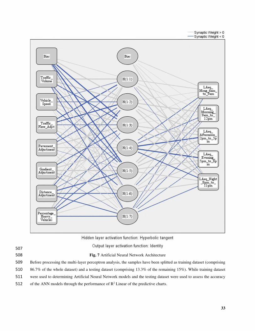
Fig. 7 Artificial Neural Network Architecture 508
Before processing the multi-layer perceptron analysis, the samples have been splitted as training dataset (comprising 509
86.7% of the whole dataset) and a testing dataset (comprising 13.3% of the remaining 15%). While training dataset 510
were used to determining Artificial Neural Network models and the testing dataset were used to assess the accuracy 511
of the ANN models through the performance of R2 Linear of the predictive charts. 512
34
513
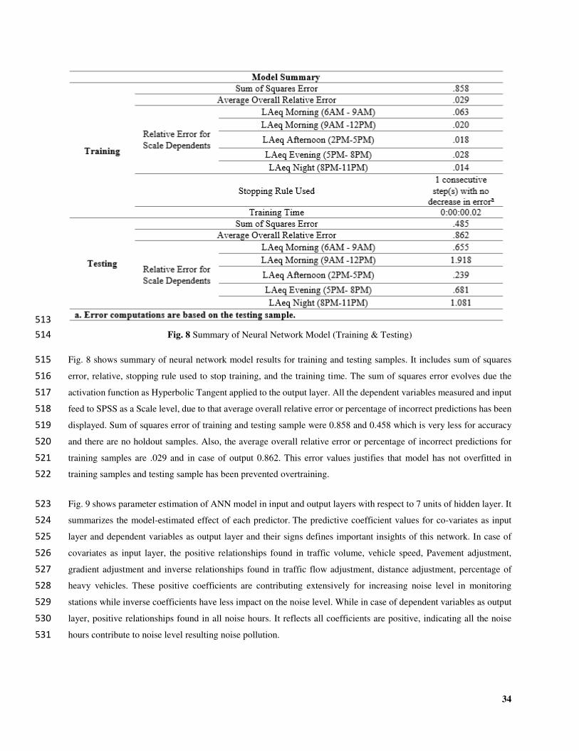
Fig. 8 Summary of Neural Network Model (Training & Testing) 514
Fig. 8 shows summary of neural network model results for training and testing samples. It includes sum of squares 515
error, relative, stopping rule used to stop training, and the training time. The sum of squares error evolves due the 516
activation function as Hyperbolic Tangent applied to the output layer. All the dependent variables measured and input 517
feed to SPSS as a Scale level, due to that average overall relative error or percentage of incorrect predictions has been 518
displayed. Sum of squares error of training and testing sample were 0.858 and 0.458 which is very less for accuracy 519
and there are no holdout samples. Also, the average overall relative error or percentage of incorrect predictions for 520
training samples are .029 and in case of output 0.862. This error values justifies that model has not overfitted in 521
training samples and testing sample has been prevented overtraining. 522
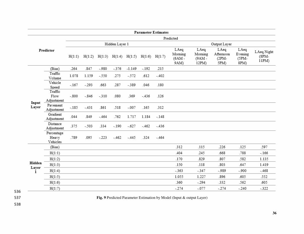
Fig. 9 shows parameter estimation of ANN model in input and output layers with respect to 7 units of hidden layer. It 523
summarizes the model-estimated effect of each predictor. The predictive coefficient values for co-variates as input 524
layer and dependent variables as output layer and their signs defines important insights of this network. In case of 525
covariates as input layer, the positive relationships found in traffic volume, vehicle speed, Pavement adjustment, 526
gradient adjustment and inverse relationships found in traffic flow adjustment, distance adjustment, percentage of 527
heavy vehicles. These positive coefficients are contributing extensively for increasing noise level in monitoring 528
stations while inverse coefficients have less impact on the noise level. While in case of dependent variables as output 529
layer, positive relationships found in all noise hours. It reflects all coefficients are positive, indicating all the noise 530
hours contribute to noise level resulting noise pollution. 531
35
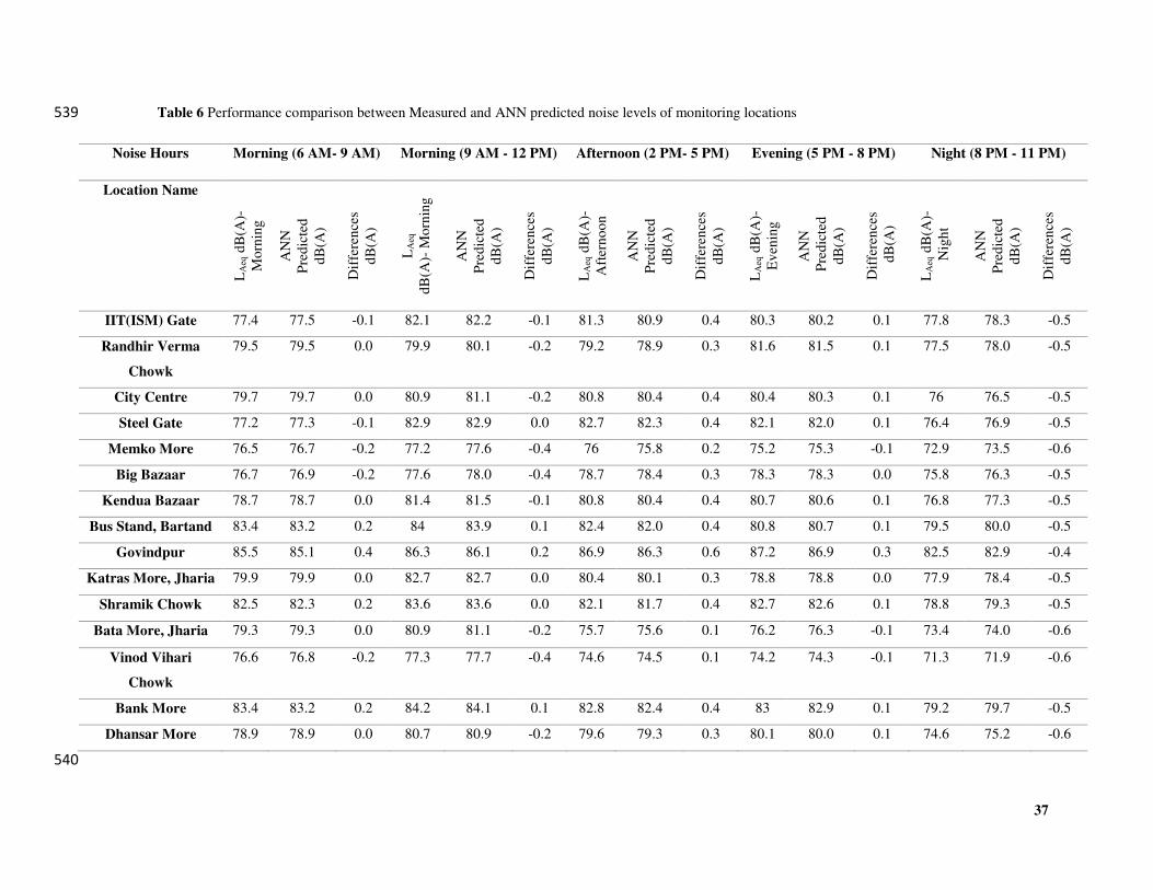
Hence it is evident from all these above interpretations that, this neural network estimated the predictive coefficients 532
are significant. Table 6 showing the performance comparison of Artificial Neural network predictions with measured 533
noise levels.534
535
36
536
Fig. 9 Predicted Parameter Estimation by Model (Input & output Layer) 537
538
37
Table 6 Performance comparison between Measured and ANN predicted noise levels of monitoring locations 539
Noise Hours Morning (6 AM- 9 AM) Morning (9 AM - 12 PM) Afternoon (2 PM- 5 PM) Evening (5 PM - 8 PM) Night (8 PM - 11 PM)
Location Name
LA
eqd
B(A
)-
Mo
rnin
g
AN
N
Pre
dic
ted
dB
(A)
Dif
fere
nce
s
dB
(A)
LA
eq
dB
(A)-
Mo
rnin
g
AN
N
Pre
dic
ted
dB
(A)
Dif
fere
nce
s
dB
(A)
LA
eqd
B(A
)-
Aft
ern
oo
n
AN
N
Pre
dic
ted
dB
(A)
Dif
fere
nce
s
dB
(A)
LA
eqd
B(A
)-
Ev
enin
g
AN
N
Pre
dic
ted
dB
(A)
Dif
fere
nce
s
dB
(A)
LA
eqd
B(A
)-
Nig
ht
AN
N
Pre
dic
ted
dB
(A)
Dif
fere
nce
s
dB
(A)
IIT(ISM) Gate 77.4 77.5 -0.1 82.1 82.2 -0.1 81.3 80.9 0.4 80.3 80.2 0.1 77.8 78.3 -0.5
Randhir Verma
Chowk
79.5 79.5 0.0 79.9 80.1 -0.2 79.2 78.9 0.3 81.6 81.5 0.1 77.5 78.0 -0.5
City Centre 79.7 79.7 0.0 80.9 81.1 -0.2 80.8 80.4 0.4 80.4 80.3 0.1 76 76.5 -0.5
Steel Gate 77.2 77.3 -0.1 82.9 82.9 0.0 82.7 82.3 0.4 82.1 82.0 0.1 76.4 76.9 -0.5
Memko More 76.5 76.7 -0.2 77.2 77.6 -0.4 76 75.8 0.2 75.2 75.3 -0.1 72.9 73.5 -0.6
Big Bazaar 76.7 76.9 -0.2 77.6 78.0 -0.4 78.7 78.4 0.3 78.3 78.3 0.0 75.8 76.3 -0.5
Kendua Bazaar 78.7 78.7 0.0 81.4 81.5 -0.1 80.8 80.4 0.4 80.7 80.6 0.1 76.8 77.3 -0.5
Bus Stand, Bartand 83.4 83.2 0.2 84 83.9 0.1 82.4 82.0 0.4 80.8 80.7 0.1 79.5 80.0 -0.5
Govindpur 85.5 85.1 0.4 86.3 86.1 0.2 86.9 86.3 0.6 87.2 86.9 0.3 82.5 82.9 -0.4
Katras More, Jharia 79.9 79.9 0.0 82.7 82.7 0.0 80.4 80.1 0.3 78.8 78.8 0.0 77.9 78.4 -0.5
Shramik Chowk 82.5 82.3 0.2 83.6 83.6 0.0 82.1 81.7 0.4 82.7 82.6 0.1 78.8 79.3 -0.5
Bata More, Jharia 79.3 79.3 0.0 80.9 81.1 -0.2 75.7 75.6 0.1 76.2 76.3 -0.1 73.4 74.0 -0.6
Vinod Vihari
Chowk
76.6 76.8 -0.2 77.3 77.7 -0.4 74.6 74.5 0.1 74.2 74.3 -0.1 71.3 71.9 -0.6
Bank More 83.4 83.2 0.2 84.2 84.1 0.1 82.8 82.4 0.4 83 82.9 0.1 79.2 79.7 -0.5
Dhansar More 78.9 78.9 0.0 80.7 80.9 -0.2 79.6 79.3 0.3 80.1 80.0 0.1 74.6 75.2 -0.6
540
38
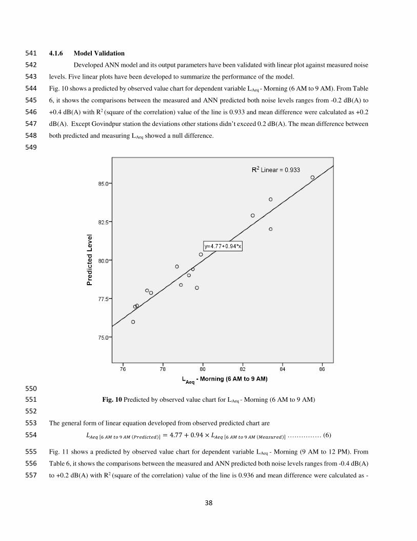
4.1.6 Model Validation 541
Developed ANN model and its output parameters have been validated with linear plot against measured noise 542
levels. Five linear plots have been developed to summarize the performance of the model. 543
Fig. 10 shows a predicted by observed value chart for dependent variable LAeq - Morning (6 AM to 9 AM). From Table 544
6, it shows the comparisons between the measured and ANN predicted both noise levels ranges from -0.2 dB(A) to 545
+0.4 dB(A) with R2 (square of the correlation) value of the line is 0.933 and mean difference were calculated as +0.2 546
dB(A). Except Govindpur station the deviations other stations didn’t exceed 0.2 dB(A). The mean difference between 547
both predicted and measuring LAeq showed a null difference. 548
549
550
Fig. 10 Predicted by observed value chart for LAeq - Morning (6 AM to 9 AM) 551
552
The general form of linear equation developed from observed predicted chart are 553 𝐿𝐴𝑒𝑞 [6 𝐴𝑀 𝑡𝑜 9 𝐴𝑀 (𝑃𝑟𝑒𝑑𝑖𝑐𝑡𝑒𝑑)] = 4.77 + 0.94 × 𝐿𝐴𝑒𝑞 [6 𝐴𝑀 𝑡𝑜 9 𝐴𝑀 (𝑀𝑒𝑎𝑠𝑢𝑟𝑒𝑑)] …………… (6) 554
Fig. 11 shows a predicted by observed value chart for dependent variable LAeq - Morning (9 AM to 12 PM). From 555
Table 6, it shows the comparisons between the measured and ANN predicted both noise levels ranges from -0.4 dB(A) 556
to +0.2 dB(A) with R2 (square of the correlation) value of the line is 0.936 and mean difference were calculated as -557
39
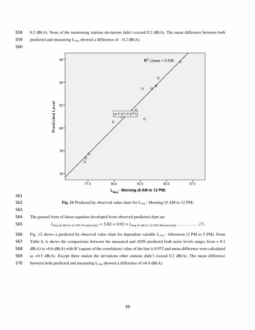
0.2 dB(A). None of the monitoring stations deviations didn’t exceed 0.2 dB(A). The mean difference between both 558
predicted and measuring LAeq showed a difference of – 0.2 dB(A). 559
560
561
Fig. 11 Predicted by observed value chart for LAeq - Morning (9 AM to 12 PM) 562
563
The general form of linear equation developed from observed predicted chart are 564 𝐿𝐴𝑒𝑞 [9 𝐴𝑀 𝑡𝑜 12 𝑃𝑀 (𝑃𝑟𝑒𝑑𝑖𝑐𝑡𝑒𝑑)] = 5.82 + 0.93 × 𝐿𝐴𝑒𝑞 [9 𝐴𝑀 𝑡𝑜 12 𝑃𝑀 (𝑀𝑒𝑎𝑠𝑢𝑟𝑒𝑑)] …………… (7) 565
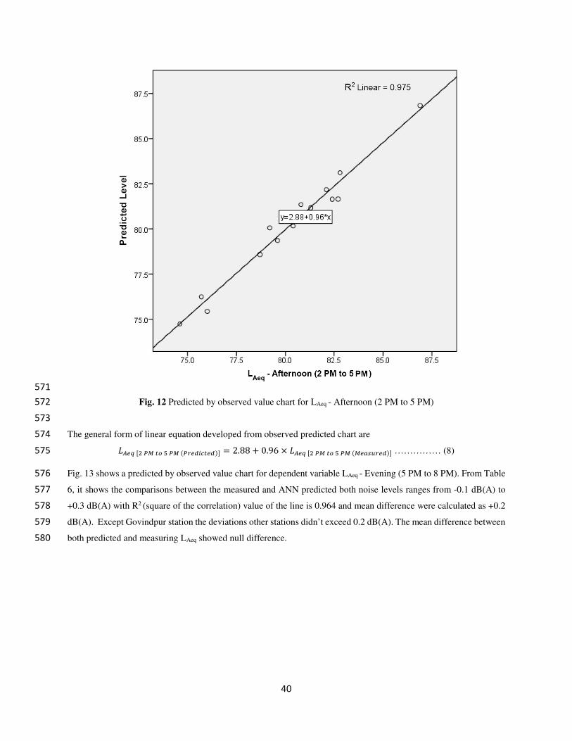
Fig. 12 shows a predicted by observed value chart for dependent variable LAeq - Afternoon (2 PM to 5 PM). From 566
Table 6, it shows the comparisons between the measured and ANN predicted both noise levels ranges from + 0.1 567
dB(A) to +0.6 dB(A) with R2 (square of the correlation) value of the line is 0.975 and mean difference were calculated 568
as +0.5 dB(A). Except three station the deviations other stations didn’t exceed 0.2 dB(A). The mean difference 569
between both predicted and measuring LAeq showed a difference of +0.4 dB(A). 570
40
571
Fig. 12 Predicted by observed value chart for LAeq - Afternoon (2 PM to 5 PM) 572
573
The general form of linear equation developed from observed predicted chart are 574 𝐿𝐴𝑒𝑞 [2 𝑃𝑀 𝑡𝑜 5 𝑃𝑀 (𝑃𝑟𝑒𝑑𝑖𝑐𝑡𝑒𝑑)] = 2.88 + 0.96 × 𝐿𝐴𝑒𝑞 [2 𝑃𝑀 𝑡𝑜 5 𝑃𝑀 (𝑀𝑒𝑎𝑠𝑢𝑟𝑒𝑑)] …………… (8) 575
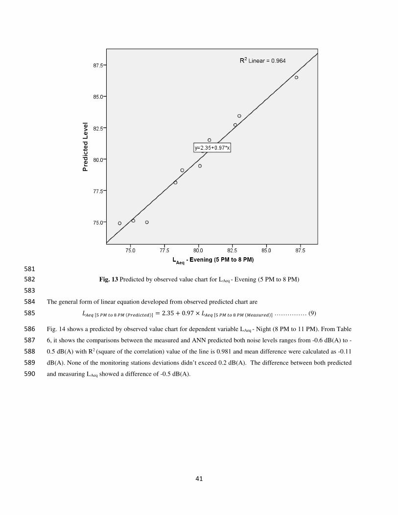
Fig. 13 shows a predicted by observed value chart for dependent variable LAeq - Evening (5 PM to 8 PM). From Table 576
6, it shows the comparisons between the measured and ANN predicted both noise levels ranges from -0.1 dB(A) to 577
+0.3 dB(A) with R2 (square of the correlation) value of the line is 0.964 and mean difference were calculated as +0.2 578
dB(A). Except Govindpur station the deviations other stations didn’t exceed 0.2 dB(A). The mean difference between 579
both predicted and measuring LAeq showed null difference. 580
41
581
Fig. 13 Predicted by observed value chart for LAeq - Evening (5 PM to 8 PM) 582
583
The general form of linear equation developed from observed predicted chart are 584 𝐿𝐴𝑒𝑞 [5 𝑃𝑀 𝑡𝑜 8 𝑃𝑀 (𝑃𝑟𝑒𝑑𝑖𝑐𝑡𝑒𝑑)] = 2.35 + 0.97 × 𝐿𝐴𝑒𝑞 [5 𝑃𝑀 𝑡𝑜 8 𝑃𝑀 (𝑀𝑒𝑎𝑠𝑢𝑟𝑒𝑑)] …………… (9) 585
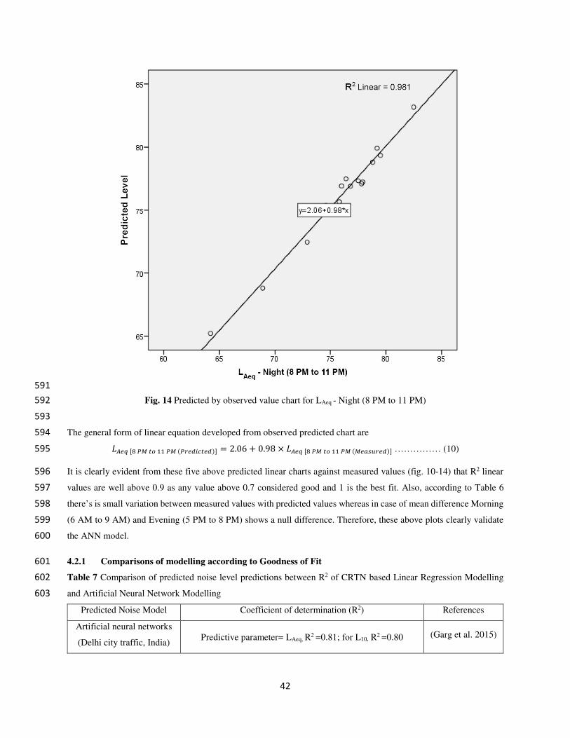
Fig. 14 shows a predicted by observed value chart for dependent variable LAeq - Night (8 PM to 11 PM). From Table 586
6, it shows the comparisons between the measured and ANN predicted both noise levels ranges from -0.6 dB(A) to -587
0.5 dB(A) with R2 (square of the correlation) value of the line is 0.981 and mean difference were calculated as -0.11 588
dB(A). None of the monitoring stations deviations didn’t exceed 0.2 dB(A). The difference between both predicted 589
and measuring LAeq showed a difference of -0.5 dB(A). 590
42
591
Fig. 14 Predicted by observed value chart for LAeq - Night (8 PM to 11 PM) 592
593
The general form of linear equation developed from observed predicted chart are 594 𝐿𝐴𝑒𝑞 [8 𝑃𝑀 𝑡𝑜 11 𝑃𝑀 (𝑃𝑟𝑒𝑑𝑖𝑐𝑡𝑒𝑑)] = 2.06 + 0.98 × 𝐿𝐴𝑒𝑞 [8 𝑃𝑀 𝑡𝑜 11 𝑃𝑀 (𝑀𝑒𝑎𝑠𝑢𝑟𝑒𝑑)] …………… (10) 595
It is clearly evident from these five above predicted linear charts against measured values (fig. 10-14) that R2 linear 596
values are well above 0.9 as any value above 0.7 considered good and 1 is the best fit. Also, according to Table 6 597
there’s is small variation between measured values with predicted values whereas in case of mean difference Morning 598
(6 AM to 9 AM) and Evening (5 PM to 8 PM) shows a null difference. Therefore, these above plots clearly validate 599
the ANN model. 600
4.2.1 Comparisons of modelling according to Goodness of Fit 601
Table 7 Comparison of predicted noise level predictions between R2 of CRTN based Linear Regression Modelling 602
and Artificial Neural Network Modelling 603
Predicted Noise Model Coefficient of determination (R2) References
Artificial neural networks
(Delhi city traffic, India) Predictive parameter= LAeq, R2 =0.81; for L10, R2 =0.80 (Garg et al. 2015)
43
Open source Traffic Noise
Exposure model
(TRANEX) (Leicester and
Norwich, UK)
Predictive parameter= LAeq,1hr. for Norwich, R2 =0.85 and
Leicester, R2 =0.95
(Gulliver et al.
2015)
Neural Networks (Patiala
city traffic, Punjab, India) Predictive parameter= Leq, R2 =0.83 and for L10, R2 =0.80 (Singh et al. 2016)
CRTN based Linear
Regression Modelling
(Dhanbad town road
networks, Jharkhand)
Predictive parameter= LAeq,. R2Morning (6AM-9AM) =0.74 R2
Morning
(9AM-12PM) = 0.81, R2Afternoon (2PM-5PM) =0.71, R2
Evening (5PM-8PM) =
0.69, R2Night (8PM-11PM) =0.60
(Debnath and
Singh, 2018)
Modified Federal Highway
Administration (FHWA)
model (Nagpur City road
traffic, India)
Predictive parameter= Leq, R2 =0.457 for morning and
evening peak hours
(Pathak et al.
2018)
Traffic noise evaluation
model (TNEM) (Nanguan
District, China)
Predictive parameter= LA (instantaneous sound level), R2 =0.86 (Di et al. 2018)
Emotional Artificial
Neural Network (EANN)
(Nicosia, North Cyprus)
Predictive parameter= Leq, R2 =0.80 (Nourani et al.
2020)
Artificial Neural Network
(Chongqing city, China) Predictive parameter= Leq, R2 =0.827 (Chen et al. 2020)
Artificial Neural Network
Modelling (Dhanbad town,
India)
Predictive parameter= LAeq,. R2Morning (6AM-9AM) =0.933 R2
Morning
(9AM-12PM) = 0.936, R2Afternoon (2PM-5PM) =0.975, R2
Evening (5PM-8PM)
= 0.964, R2Night (8PM-11PM) =0.981
Present study
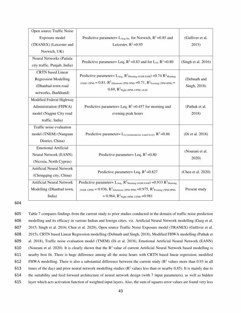
604
Table 7 compares findings from the current study to prior studies conducted in the domain of traffic noise prediction 605
modelling and its efficacy in various Indian and foreign cities. viz. Artificial Neural Network modelling (Garg et al. 606
2015; Singh et al. 2016; Chen et al. 2020), Open source Traffic Noise Exposure model (TRANEX) (Gulliver et al. 607
2015), CRTN based Linear Regression modelling (Debnath and Singh, 2018), Modified FHWA modelling (Pathak et 608
al. 2018), Traffic noise evaluation model (TNEM) (Di et al. 2018), Emotional Artificial Neural Network (EANN) 609
(Nourani et al. 2020). It is clearly shown that the R2 value of current Artificial Neural Network based modelling is 610
nearby best fit. There is huge difference among all the noise hours with CRTN based linear regression, modified 611
FHWA modelling. There is also a substantial difference between the current study (R2 values more than 0.93 in all 612
times of the day) and prior neural network modelling studies (R2 values less than or nearby 0.85). It is mainly due to 613
the suitability and feed forward architecture of neural network design (with 7 input parameters), as well as hidden 614
layer which acts activation function of weighted input layers. Also, the sum of squares error values are found very less 615
44
in training and testing of network. The comparison of the predicted values and measured values shown in Table 6 616
suggests that there is less difference up to ±0.6 dB(A), which also validates the proposed ANN model. 617
From the above result of radial noise diagrams it is clearly visible that except some maximum station has exceeded 618
the permissible limit of ambient noise standards for industrial, commercial, residential and silence area has been 619
notified under The Noise Pollution (Regulation and Control) Rules, 2000 (Ministry of Environment and Forests 2000) 620
by Ministry of Environment & Forest, Govt. of India which is discussed in the literature section. Contour plotting 621
shows the relationship between vehicle speed and traffic volume to act as a driving factor for increasing or decreasing 622
noise levels. The values of different noise descriptors shows the annoyance and disturbing effects, and noise level 623
during 10% & 90% exceeded of time. Also as discussed, the rationale behind using this ANN modelling in literature 624
section and comparisons with regression modelling shows that the performance of this model complies with the 625
existing literatures and their findings.626
5.1 Conclusions 627
This study finds suitability of artificial neural network model in Dhanbad township for road traffic noise 628
modelling and it has successfully predicted LAeq noise levels. This present study highlights the vehicular road traffic 629
situation of Dhanbad township by analyzing average noise level based radial figures, noise descriptors and indexes 630
(L10, L90, 24hrs Ldn, LNP, TNI NC) and contour plots (noise level against traffic volume and speed). Following Some 631
conclusions have been drawn from this study- 632
1. In this paper, we found that the average noise levels of all the stations beyond permissible limit given by under The 633
Noise Pollution (Regulation and Control) Rules, 2000 of Environment (Protection) Act in both peak and non-peak 634
hours. It can be observed that levels were slightly improved during afternoon and night hours. 635
2. From traffic flow characterization it’s clear that that flow are heterogenous where more than 59% vehicles were 636
two-wheelers, following by 19.37% four-wheelers, 1.22% buses & trekkers, and morning hours (9 AM to 12 PM) has 637
the highest & night hour has the lowest flow of vehicles recorded all over the Dhanbad township. 638
3. In case of noise descriptors, Govindpur has highest levels of L10, L90 among the others. It is evident that from 639
observed values that as the traffic volume increases noise level simultaneously increases, the peak levels increase over 640
the time duration due to honking of vehicles in heavy traffic areas. Ldn levels of several stations found more than 85 641
dB(A). The TNI and LNP values are much higher, ranges between 100-200 dB(A), even in some points it goes beyond 642
200 dB(A) which indicates that high annoyance level, variations in flow in Dhanbad township While NC fluctuation 643
level goes up to 45 dB(A). 644
4. From these contour plots, it has been observed that highest noise levels were found at the speed of 50-55 km/h in 645
all peak and non-peak hours. The lowest noise levels were found in the shallow streams of the contour with at an 646
average traffic volume of less than 2000 or less. Also, plot suggests that the noise level crucial at a speed of 20-30 and 647
45-55 km/h in peak and non-peak hours where the level crosses 80 dB(A) with an traffic volume between 5000-10000. 648
45
5. In this paper, multilayer perceptron neural network has been applied for prediction of noise level. A network 649
architecture with 7-7-5 formation has been processed with user friendly SPSS 21.0 software package and model found 650
as optimum due to its performance in training and testing phase, less sum of square and % of incorrect prediction 651
errors. The obtained results from ANN showed that the deviation are up to ±0.6 dB(A) compared with the measured 652
noise levels. Furthermore, the comparisons between the outputs of ANN and regression based CRTN modelling 653
(Debnath and Singh, 2018), it is found that the R2 linear values of ANN modelling of all the noise hours are more than 654
0.9 which is nearby best fit and it could be concluded that ANN shows much better capabilities to predict equivalent 655
noise level based on the traffic flow structure than regression modelling in terms of predictive performance of 656
correlation coefficient. 657
Following several future recommendations also can be made to reduce road traffic noise and usability of the model. 658
a) Proper management of heavy vehicles including trucks & buses and construction of noise barrier’s in road 659
intersections which will obstruct the noise level at some extent. 660
b) For better traffic flow management, it will highly advisable that municipality or Gov. urban bodies should 661
install speed bar banner written up to 35-45 km/h Max speed in city areas or road intersections. 662
c) These contour plots can effective for future scenario prediction by policy and decision makers, town planners, 663
municipality and urban bodies and other private stakeholders for road traffic noise management. 664
d) Use of low noise road surfaces (asphalt road surfaces) is the viable solution to mitigate the noise emitted 665
from tyre-road interaction. 666
e) This model can help as a useful tool to integrate acoustical variables for urban planners and engineers in 667
future traffic planning, redesigning traffic patterns, slip-roads, fly-overs as a mitigative measure for noise 668
reduction. It will lead to develop future action plans in terms of reduction. 669
f) The researchers also recommend future research to include more variables or factors as descriptors and 670
indexes viz. L10, L90, 24hrs Ldn, LNP, TNI, NC in a macroscopic approach to develop more comprehensive 671
network model archiving more significant results. 672
6.1 Declarations 673
6.1.1 Ethics approval and consent to participate: Not Applicable. 674
6.1.2 Consent to Publish: Not Applicable.675
6.1.3 Availability of data and materials: All data generated or analysed during this study are included in this 676
published article. 677
6.1.4 Competing interests: The authors declare that they have no known competing interests. 678
6.1.5 Funding: The authors declare that no financial support received for this work that could have influenced its 679
outcome. 680
6.1.6 Authors' contributions: Conceptualization, Methodology, Writing - original draft, Formal analysis, 681
Validation have been done by Author 1 (Abhijit Debnath). The work has been supervised by the Author 2 (Prasoon 682
Kumar Singh) and drafted manuscript has been reviewed and edited by Author 3 (Sushmita Banerjee). 683
46
6.1.6 Acknowledgements: The authors are sincerely thankful to Department of Environment Science & 684
Engineering, Indian Institute of Technology (Indian School of Mines), Dhanbad and for providing facilities, guidance 685
and co-operation carrying out the work. 686
7.1 References 687
Acoustical Society of Japan (1999) ASJ Prediction model 1998 for road traffic noise: Report from the research 688
committee of Road Traffic Noise in the Acoustical Society of Japan 689
Agarwal S, Swami BL (2010) Noise Annoyance under Interrupted Traffic Flow Condition for Jaipur City. Int J Appl 690
Sci Eng 7:159–168 691
Avşar Y, Saral A, Gönüllü MT, et al (2004) Neural network modelling of outdoor noise levels in a pilot area. Turkish 692
J Eng Environ Sci 28:149–155. https://doi.org/10.3906/sag-1204-111 693
Babisch W, Beule B, Schust M, et al (2005) Traffic noise and risk of myocardial infarction. Epidemiology 16:33–40. 694
https://doi.org/10.1097/01.ede.0000147104.84424.24 695
Bahadure S, Kotharkar R (2018) Framework for measuring sustainability of neighbourhoods in Nagpur, India. Build 696
Environ 127:86–97. https://doi.org/10.1016/j.buildenv.2017.10.034 697
Banerjee D, Chakraborty SK, Bhattacharyya S, Gangopadhyay A (2008a) Modeling of road traffic noise in the 698
industrial town of Asansol, India. Transp Res Part D Transp Environ 13:539–541. 699
https://doi.org/10.1016/j.trd.2008.09.008 700
Banerjee D, Chakraborty SK, Bhattacharyya S, Gangopadhyay A (2008b) Evaluation and analysis of road traffic noise 701
in asansol, West Bengal. J Inst Eng Environ Eng Div 89:9–16 702
Basner M, McGuire S (2018) WHO Environmental Noise Guidelines for the European Region: A Systematic Review 703
on Environmental Noise and Effects on Sleep. Int J Environ Res Public Health 15:519. 704
https://doi.org/10.3390/ijerph15030519 705
Bastián-Monarca NA, Suárez E, Arenas JP (2016) Assessment of methods for simplified traffic noise mapping of 706
small cities: Casework of the city of Valdivia, Chile. Sci Total Environ 550:439–448. 707
https://doi.org/10.1016/j.scitotenv.2016.01.139 708
Bianco F, Fredianelli L, Lo Castro F, et al (2020) Stabilization of a p-u sensor mounted on a vehicle for measuring 709
the acoustic impedance of road surfaces. Sensors (Switzerland) 20:1–16. https://doi.org/10.3390/s20051239 710
Boodihal MA, Chethan A, Swamy R, et al (2014) Development of tyre/road noise assessment methodology in India. 711
Case Stud Constr Mater 1:115–124. https://doi.org/10.1016/j.cscm.2014.06.001 712
Bravo-Moncayo L, Lucio-Naranjo J, Chávez M, et al (2019) A machine learning approach for traffic-noise annoyance 713
assessment. Appl Acoust 156:262–270. https://doi.org/10.1016/j.apacoust.2019.07.010 714
Brown AL, De Coensel B (2018) A study of the performance of a generalized exceedance algorithm for detecting 715
noise events caused by road traffic. Appl Acoust 138:101–114. 716
https://doi.org/10.1016/j.apacoust.2018.03.031 717
Cai P, Wang Y, Lu G, et al (2016) A spatiotemporal correlative k-nearest neighbor model for short-term traffic 718
multistep forecasting. Transp Res Part C Emerg Technol. https://doi.org/10.1016/j.trc.2015.11.002 719
47
Cammarata G, Cavalieri S, Fichera A (1995) A neural network architecture for noise prediction. Neural Networks. 720
https://doi.org/10.1016/0893-6080(95)00016-S 721
Chen L, Tang B, Liu T, et al (2020) Modeling traffic noise in a mountainous city using artificial neural networks and 722
gradient correction. Transp Res Part D Transp Environ 78:102196. https://doi.org/10.1016/j.trd.2019.11.025 723
Chowdhury AK, Debsarkar A, Chakrabarty S (2012) Analysis of day time traffic noise level : A case study of Kolkata, 724
India. Int J Environ Sci Res 2:114–118 725
De Coensel B, Brown AL, Tomerini D (2016) A road traffic noise pattern simulation model that includes distributions 726
of vehicle sound power levels. Appl Acoust 111:170–178. https://doi.org/10.1016/j.apacoust.2016.04.010 727
de León G, Del Pizzo A, Teti L, et al (2020) Evaluation of tyre/road noise and texture interaction on rubberised and 728
conventional pavements using CPX and profiling measurements. Road Mater Pavement Des 21:S91–S102. 729
https://doi.org/10.1080/14680629.2020.1735493 730
Debnath A, Singh PK (2018) Environmental traffic noise modelling of Dhanbad township area – A mathematical 731
based approach. Appl Acoust 129:161–172. https://doi.org/10.1016/j.apacoust.2017.07.023 732
Del Pizzo A, Teti L, Moro A, et al (2020) Influence of texture on tyre road noise spectra in rubberized pavements. 733
Appl Acoust 159:107080. https://doi.org/10.1016/j.apacoust.2019.107080 734
Di H, Liu X, Zhang J, et al (2018) Estimation of the quality of an urban acoustic environment based on traffic noise 735
evaluation models. Appl Acoust 141:115–124. https://doi.org/10.1016/j.apacoust.2018.07.010 736
Dratva J, Phuleria HC, Foraster M, et al (2012) Transportation noise and blood pressure in a population-based sample 737
of adults. Environ Health Perspect 120:50–55. https://doi.org/10.1289/ehp.1103448 738
Dzhambov A, Tilov B, Markevych I, Dimitrova D (2017) Residential road traffic noise and general mental health in 739
youth: The role of noise annoyance, neighborhood restorative quality, physical activity, and social cohesion 740
as potential mediators. Environ Int. https://doi.org/10.1016/j.envint.2017.09.009 741
Erickson LC, Newman RS (2017) Influences of Background Noise on Infants and Children. Curr Dir Psychol Sci 742
26:451–457. https://doi.org/10.1177/0963721417709087 743
Estévez-Mauriz L, Forssén J (2018) Dynamic traffic noise assessment tool: A comparative study between a 744
roundabout and a signalised intersection. Appl Acoust 130:71–86. 745
https://doi.org/10.1016/j.apacoust.2017.09.003 746
FHWA Traffic Noise Model (1998) Technical manual, FHWA-PD-96-010 747
Garg N, Mangal SK, Saini PK, et al (2015) Comparison of ANN and Analytical Models in Traffic Noise Modeling 748
and Predictions. Acoust Aust 43:179–189. https://doi.org/10.1007/s40857-015-0018-3 749
Gilani TA, Mir MS (2021a) Association of road traffic noise exposure and prevalence of coronary artery disease: A 750
cross-sectional study in North India. Environ Sci Pollut Res. https://doi.org/10.1007/s11356-021-14582-2 751
Gilani TA, Mir MS (2021b) A study on the assessment of traffic noise induced annoyance and awareness levels about 752
the potential health effects among residents living around a noise-sensitive area. Environ Sci Pollut Res Int. 753
https://doi.org/10.1007/s11356-021-15208-3 754
Gilani TA, Mir MS (2021c) Modelling road traffic Noise under heterogeneous traffic conditions using the graph-755
theoretic approach. Environ Sci Pollut Res. https://doi.org/10.1007/s11356-021-13328-4 756
48
Givargis S, Karimi H (2010) A basic neural traffic noise prediction model for Tehran’s roads. J Environ Manage 757
91:2529–2534. https://doi.org/10.1016/j.jenvman.2010.07.011 758
Givargis S, Mahmoodi M (2008) Converting the UK calculation of road traffic noise (CORTN) to a model capable of 759
calculating LAeq,1h for the Tehran’s roads. Appl Acoust. https://doi.org/10.1016/j.apacoust.2007.08.003 760
Golmohammadi R, Abbaspour M, Nassiri P, Mahjub H (2009) A compact model for predicting road traffic noise. Iran 761
J Environ Heal Sci Eng 6:181–186 762
Gulliver J, Morley D, Vienneau D, et al (2015) Development of an open-source road traffic noise model for exposure 763
assessment. Environ Model Softw 74:183–193. https://doi.org/10.1016/j.envsoft.2014.12.022 764
Habtemichael FG, Cetin M (2016) Short-term traffic flow rate forecasting based on identifying similar traffic patterns. 765
Transp Res Part C Emerg Technol. https://doi.org/10.1016/j.trc.2015.08.017 766
Hamad K, Ali Khalil M, Shanableh A (2017) Modeling roadway traffic noise in a hot climate using artificial neural 767
networks. Transp Res Part D Transp Environ 53:161–177. https://doi.org/10.1016/j.trd.2017.04.014 768
Hamed MM, Ai-Masaeid HR, Bani Said ZM (1995) Short-term prediction of traffic volume in urban arterials. J Transp 769
Eng. https://doi.org/10.1061/(ASCE)0733-947X(1995)121:3(249) 770
Heidemann C, Niemann H, Paprott R, et al (2014) Residential traffic and incidence of type 2 diabetes: The german 771
health interview and examination surveys. Diabet Med. https://doi.org/10.1111/dme.12480 772
Huang B, Pan Z, Liu Z, et al (2017) Acoustic amenity analysis for high-rise building along urban expressway: 773
Modeling traffic noise vertical propagation using neural networks. Transp Res Part D Transp Environ 53:63–774
77. https://doi.org/10.1016/j.trd.2017.04.001 775
Jha MK, Kang MW (2009) GIS-Based Model for Highway Noise Analysis. J Infrastruct Syst 15:88–94. 776
https://doi.org/10.1061/(asce)1076-0342(2009)15:2(88) 777
Kalaiselvi R, Ramachandraiah A (2016) Honking noise corrections for traffic noise prediction models in 778
heterogeneous traffic conditions like India. Appl Acoust 111:25–38. 779
https://doi.org/10.1016/j.apacoust.2016.04.003 780
Khan V, Biligiri KP (2018) Evolution of tyre/road noise research in India: Investigations using statistical pass-by 781
method and noise trailer. Int J Pavement Res Technol 11:253–264. 782
https://doi.org/10.1016/j.ijprt.2017.09.018 783
Klæboe R, Engelien E, Steinnes M (2006) Context sensitive noise impact mapping. Appl Acoust 67:620–642. 784
https://doi.org/10.1016/j.apacoust.2005.12.002 785
Konbattulwar V, Velaga NR, Jain S, Sharmila RB (2016) Development of in-vehicle noise prediction models for 786
Mumbai Metropolitan Region, India. J Traffic Transp Eng (English Ed 3:380–387. 787
https://doi.org/10.1016/j.jtte.2016.04.002 788
Kumar P, Nigam SP, Kumar N (2014) Vehicular traffic noise modeling using artificial neural network approach. 789
Transp Res Part C Emerg Technol 40:111–122. https://doi.org/10.1016/j.trc.2014.01.006 790
Laxmi V, Dey J, Kalawapudi K, et al (2019) An innovative approach of urban noise monitoring using cycle in Nagpur, 791
India. Environ Sci Pollut Res 26:36812–36819. https://doi.org/10.1007/s11356-019-06817-0 792
49
Licitra G, Fredianelli L, Petri D, Vigotti MA (2016) Annoyance evaluation due to overall railway noise and vibration 793
in Pisa urban areas. Sci Total Environ 568:1315–1325. https://doi.org/10.1016/j.scitotenv.2015.11.071 794
Licitra G, Teti L, Cerchiai M, Bianco F (2017) The influence of tyres on the use of the CPX method for evaluating 795
the effectiveness of a noise mitigation action based on low-noise road surfaces. Transp Res Part D Transp 796
Environ 55:217–226. https://doi.org/10.1016/j.trd.2017.07.002 797
Lv Y, Duan Y, Kang W, et al (2015) Traffic Flow Prediction with Big Data: A Deep Learning Approach. IEEE Trans 798
Intell Transp Syst. https://doi.org/10.1109/TITS.2014.2345663 799
Manojkumar N, Basha K, Srimuruganandam B (2019) Assessment, Prediction and Mapping of Noise Levels in 800
Vellore City, India. Noise Mapp. https://doi.org/10.1515/noise-2019-0004 801
Marathe PD (2012) Traffic noise pollution. Ijed 9:63–68 802
Miedema HME, Oudshoorn CGM (2001) Annoyance from transportation noise: Relationships with exposure metrics 803
DNL and DENL and their confidence intervals. Environ Health Perspect 109:409–416. 804
https://doi.org/10.1289/ehp.01109409 805
Minichilli F, Gorini F, Ascari E, et al (2018) Annoyance judgment and measurements of environmental noise: A focus 806
on italian secondary schools. Int J Environ Res Public Health 15:1–17. 807
https://doi.org/10.3390/ijerph15020208 808
Ministry of Environment and forest (2000) The Noise Pollution (Regulation and Control) Rules, 2000. 12311:1088–809
1569 810
Ministry of Environment and Forests G of I (2000) The Noise Pollution (Regulation and Control) Rules, 2000. 123: 811
Muzet A (2007) Environmental noise, sleep and health. Sleep Med Rev 11:135–142. 812
https://doi.org/10.1016/j.smrv.2006.09.001 813
Nedic V, Despotovic D, Cvetanovic S, et al (2014) Comparison of classical statistical methods and artificial neural 814
network in traffic noise prediction. Environ Impact Assess Rev 49:24–30. 815
https://doi.org/10.1016/j.eiar.2014.06.004 816
Nourani V, Gökçekuş H, Umar IK, Najafi H (2020) An emotional artificial neural network for prediction of vehicular 817
traffic noise. Sci Total Environ 707:. https://doi.org/10.1016/j.scitotenv.2019.136134 818
Paschalidou AK, Kassomenos P, Chonianaki F, Valkouma T (2019) 3-year noise monitoring and strategic noise 819
mapping in an extended motorway. Environ Sci Pollut Res. https://doi.org/10.1007/s11356-019-04966-w 820
Pathak SS, Lokhande SK, Kokate PA, Bodhe GL (2018) Assessment and Prediction of Environmental Noise 821
Generated by Road Traffic in Nagpur City, India. In: Singh VP, Yadav S, Yadava RN (eds) Environmental 822
Pollution, Water Science and Technology Library, 77th edn. Springer, Singapore, pp 167–180 823
Pathak V, Tripathi BD, Mishra V kumar (2008) Evaluation of traffic noise pollution and attitudes of exposed 824
individuals in working place. Atmos Environ 42:3892–3898. https://doi.org/10.1016/j.atmosenv.2007.12.070 825
Peng J, Parnell J, Kessissoglou N (2019) A six-category heavy vehicle noise emission model in free-flowing condition. 826
Appl Acoust 143:211–221. https://doi.org/10.1016/j.apacoust.2018.08.030 827
50
Petri D, Licitra G, Vigotti MA, Fredianelli L (2021) Effects of Exposure to Road, Railway, Airport and Recreational 828
Noise on Blood Pressure and Hypertension. Int J Environ Res Public Health 18:9145. 829
https://doi.org/10.3390/ijerph18179145 830
Praticò FG (2014) On the dependence of acoustic performance on pavement characteristics. Transp Res Part D Transp 831
Environ 29:79–87. https://doi.org/10.1016/j.trd.2014.04.004 832
Praticò FG, Anfosso-Lédée F (2012) Trends and Issues in Mitigating Traffic Noise through Quiet Pavements. In: 833
Procedia - Social and Behavioral Sciences. Elsevier B.V., pp 203–212 834
Praticò FG, Fedele R, Pellicano G (2021) Monitoring Road Acoustic and Mechanical Performance. In: Rizzo P, 835
Milazzo A (eds) European Workshop on Structural Health Monitoring. EWSHM 2020. Lecture Notes in 836
Civil Engineering, 127th edn. Springer, Cham, pp 594–602 837
Quartieri J, Mastorakis NE, Iannone G, et al (2009) A Review of Traffic Noise Predictive Noise Models. In: Recent 838
Advances in Applied and Theoretical Mechanics 839
Ramírez A, Domínguez E (2013) Modeling urban traffic noise with stochastic and deterministic traffic models. Appl 840
Acoust 74:614–621. https://doi.org/10.1016/j.apacoust.2012.08.001 841
Rossi L, Prato A, Lesina L, Schiavi A (2018) Effects of low-frequency noise on human cognitive performances in 842
laboratory. Build Acoust 25:17–33. https://doi.org/10.1177/1351010X18756800 843
Sandberg U, Ejsmont JA (2002) Tyre/Road Noise Reference Book. In: Kisa, Sweden ; Harg, Sweden : INFORMEX. 844
p 640 p. 845
Sharma A, Bodhe G, Schimak G (2014) Development of a traffic noise prediction model for an urban environment. 846
Noise Heal 16:63. https://doi.org/10.4103/1463-1741.127858 847
Singh D, Nigam SP, Agrawal VP, Kumar M (2016) Vehicular traffic noise prediction using soft computing approach. 848
J Environ Manage 183:59–66. https://doi.org/10.1016/j.jenvman.2016.08.053 849
Steele C (2001) Critical review of some traffic noise prediction models. Appl Acoust. https://doi.org/10.1016/S0003-850
682X(00)00030-X 851
Steinbach L, Altinsoy ME (2019) Prediction of annoyance evaluations of electric vehicle noise by using artificial 852
neural networks. Appl Acoust 145:149–158. https://doi.org/10.1016/j.apacoust.2018.09.024 853
Tan H, Wu Y, Shen B, et al (2016) Short-Term Traffic Prediction Based on Dynamic Tensor Completion. IEEE Trans 854
Intell Transp Syst. https://doi.org/10.1109/TITS.2015.2513411 855
Teti L, de León G, Del Pizzo A, et al (2020) Modelling the acoustic performance of newly laid low-noise pavements. 856
Constr Build Mater 247:118509. https://doi.org/10.1016/j.conbuildmat.2020.118509 857
Thakre C, Laxmi V, Vijay R, et al (2020) Traffic noise prediction model of an Indian road: an increased scenario of 858
vehicles and honking. Environ Sci Pollut Res. https://doi.org/10.1007/s11356-020-09923-6 859
Vijay R, Chakrabarti T, Gupta R (2018) Characterization of Traffic Noise and Honking Assessment of an Indian 860
Urban Road. Fluct Noise Lett. https://doi.org/10.1142/S0219477518500311 861
Vukić L, Mihanović V, Fredianelli L, Plazibat V (2021) Seafarers’ perception and attitudes towards noise emission 862
on board ships. Int J Environ Res Public Health 18:. https://doi.org/10.3390/ijerph18126671 863
51
Wang J, Deng W, Guo Y (2014) New Bayesian combination method for short-term traffic flow forecasting. Transp 864
Res Part C Emerg Technol. https://doi.org/10.1016/j.trc.2014.02.005 865
Wunderli JM, Pieren R, Habermacher M, et al (2016) Intermittency ratio: A metric reflecting short-term temporal 866
variations of transportation noise exposure. J Expo Sci Environ Epidemiol 26:575–585. 867
https://doi.org/10.1038/jes.2015.56 868
Zacarías FF, Molina RH, Ancela JLC, et al (2013) Noise exposure in preterm infants treated with respiratory support 869
using neonatal helmets. Acta Acust united with Acust 99:590–597. https://doi.org/10.3813/AAA.918638 870
Zannin PHT, Engel MS, Fiedler PEK, Bunn F (2013) Characterization of environmental noise based on noise 871
measurements, noise mapping and interviews: A case study at a university campus in Brazil. Cities 31:317–872
327. https://doi.org/10.1016/j.cities.2012.09.008 873