arX

iv:c

ond-

mat

/960

9064

v1 6

Sep

199

6

Variational and DMRG studies of the frustrated

antiferromagnetic Heisenberg S = 1 quantum spin chain

A. Kolezhuk

Institut fur Theoretische Physik, Universitat Hannover, 30167 Hannover, Germany

∗Institute of Magnetism, Natl. Acad. Sci. of Ukraine, 252142 Kiev, Ukraine

R. Roth and U. Schollwock

Sektion Physik, Ludwig-Maximilians-Univ. Munchen, Theresienstr. 37, 80333 Munich, Germany

(September 4, 1996)

Abstract

In this paper we study a frustrated antiferromagnetic isotropic Heisenberg

S = 1 quantum spin chain

H =∑

i

SiSi+1 + α∑

i

SiSi+2,

using a variational ansatz starting from valence bond states and the Density

Matrix Renormalization Group. We find both methods to give results in very

good qualitative and good quantitative agreement, which clarify the phase

diagram as follows: At αD = 0.284(1), there is a disorder point of the second

kind, marking the onset of incommensurate spin-spin correlations in the chain.

At αL = 0.3725(25) there is a Lifshitz point, at which the excitation spectrum

is found to develop a particular doubly degenerate structure. These points are

the quantum remnants of the transition from antiferromagnetic to spiral order

in the classical frustrated chain. At αT = 0.7444(6) there is a first order phase

transition from an Affleck-Kennedy-Lieb-Tasaki (AKLT) phase characterized

by non-vanishing string order to a phase which can be understood as a next-

nearest neighbor generalization of the AKLT model. At the transition, the

1

string order parameter shows (to numerical precision) a discontinuous jump

of 0.085 to zero; the correlation length and the gap are both finite at the

transition. The problem of edge states in open frustrated chains is discussed

at length.

75.50.Ee, 75.10.Jm, 75.40.Mg

Typeset using REVTEX

2

I. INTRODUCTION

Over the past years, frustrated quantum mechanical systems have met with considerable

interest.1 Research is concentrating on geometrically frustrated systems, where the lattice

geometry introduces competing interactions, and on systems, where frustration is directly

introduced by interaction, e.g. the additional presence of next-nearest neighbor interactions.

Interest in these systems has twofold motivation. There are experimental systems which show

geometrical frustration (quasi 1D hexagonal insulators such as CsNiCl3 or effective Kagome

lattices such as SrCr8−xGa4+xO19); there are also systems frustrated by interaction: A well-

known motivation is given by high-Tc superconductors, which exhibit an antiferromagnetic

phase. It has been shown early on that doping of these compounds may be mapped to

frustrated spin models.2 Another prominent example is CuGeO3, a one-dimensional S=1/2

antiferromagnet with strong competing interactions.3 On the other hand, there is purely

theoretical motivation to study these systems. Taking the classical limit, frustration may

introduce rather complex forms of order. Quantum fluctuations will destroy long-range order

which may be present in the classical system, if the dimension of the system is low. For one-

dimensional quantum systems, order will in general be destroyed even at zero temperature.4

It is therefore of interest to study which remnants of the classical system survive in the

quantum system, and whether there are purely quantum phenomena present. About the

simplest frustrated system conceivable is the frustrated Heisenberg isotropic quantum spin

chain with antiferromagnetic interactions between nearest and next-nearest neighbors. From

the well-established5–7 Haldane conjecture8,9 it is known that in the limit of a vanishing

next-nearest-neighbor interaction there is a fundamental difference between half-integer and

integer spin chains. The unfrustrated half-integer spin chain is characterized by almost

long-range antiferromagnetic order, with power-law correlations and a critical spectrum

ω = c(k−π) at low energies. The integer spin chain has only short-ranged antiferromagnetic

order, exponential correlations and a gapped spectrum ω = c2(k−π)2 +∆21/2, where ∆ is

the Haldane gap. We may thus expect considerably different behavior also in the frustrated

3

chains.

The case of half-integer spin chains has been extensively studied and is by now well

understood.10 The case of frustrated isotropic next-nearest neighbor integer spin chains

H =∑

i

SiSi+1 + α∑

i

SiSi+2 (1)

has also attracted considerable interest. Several scenarios and analytical and numerical stud-

ies have been proposed, in particular for S = 1. Numerical studies11,12 seem to indicate that

there is no phase transition for any value of frustration. Field theoretical studies13,14 predict

that there is always a gap for any value of frustration They indicate a doubly degenerate

excitation spectrum beyond α ≈ 0.4.14 On the other hand, it was claimed recently15,16 that

there is an almost gapless point (to numerical precision) for α = 0.73(1). The situation is

thus obscure; there is no agreement whether there is a phase transition in the chain and if

so, of which order.

In this work we study the phase diagram of a frustrated antiferromagnetic isotropic

Heisenberg quantum spin chain (1) with S = 1 at T = 0. We start with a variational

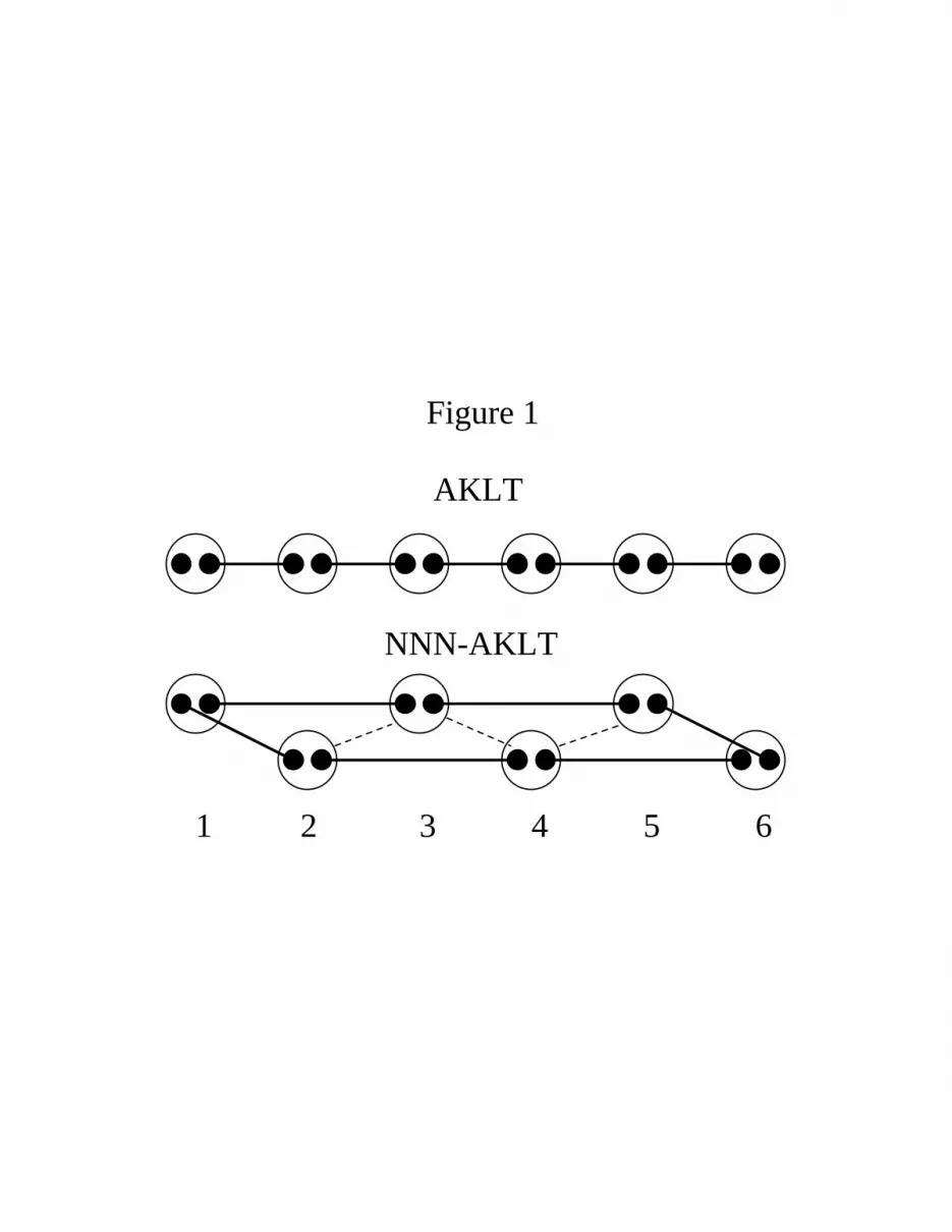
approach based on the Affleck-Kennedy-Lieb-Tasaki (AKLT)17,18 model to give analytical

predictions. Basically, two ground states are compared to each other, one being the con-

ventional AKLT model, the other an AKLT model which links next-nearest neighbors by

singlet bonds (Fig. 1). For further refinement, an ansatz interpolating between these cases

is constructed and minimized. Elementary excitations are calculated in a “crackion”19,20

picture. On the other hand, we use the Density Matrix Renormalization Group (DMRG)5,21

to obtain quantitative results and to check the variational approach. In our DMRG calcu-

lations, we typically use M = 250 block states in chains up to L = 380 sites. This by far

exceeds previous calculations15,16 in precision. We present calculations of important quanti-

ties not considered beforehand and analyze the excitation spectrum carefully. The use of a

prediction mechanism22 to accelerate the convergence of the exact diagonalization inherent

in the DMRG allows us to go up to about M = 400 in a S = 1 system on a PentiumPro

based personal computer while retaining reasonable computing speed. The structure of the

4

paper is as follows: in section II, we briefly summarize our findings; in section III, we discuss

the associated physical scenario in more detail. Sections IV and V present the analytical

and numerical calculations.

II. SUMMARY OF RESULTS

We find that there is an AKLT (Haldane) phase for αT < 0.7444(6) with a disorder

point of the second kind23 at αD = 0.284(1) (see Figs. 3 and 2) and a Lifshitz point at

αL = 0.3725(25) (see Fig. 5). The disorder point and the associated Lifshitz point can be

understood as the quantum remnants of the phase transition from antiferromagnetic to spiral

order in the classical frustrated chain. The AKLT phase can be understood in terms of the

conventional S = 1 AKLT model (Fig. 1); the associated string order parameter24 is nonzero

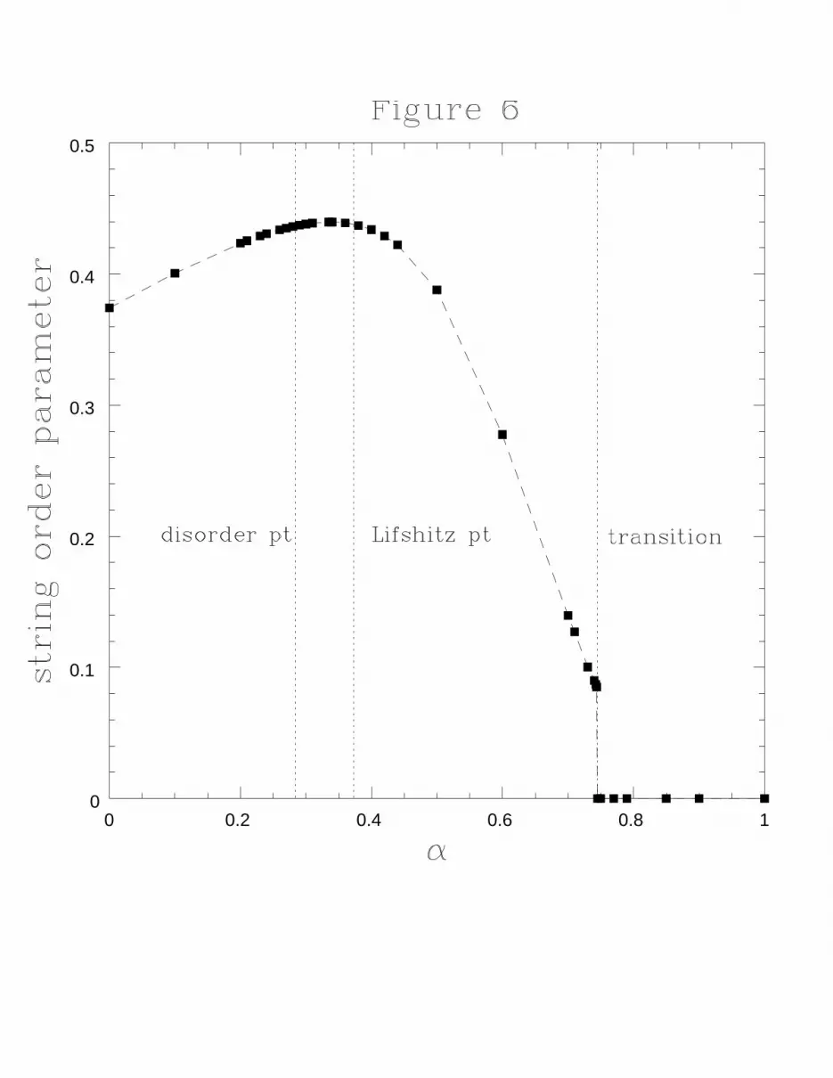
(Fig. 6), corresponding to hidden order linked to the breaking of a discrete Z2×Z2 symmetry

in the chain.25 The string order parameter shows a maximum of 0.4397(1) at α = 0.3375(25)

close to the disorder point, and disappears with a discontinuous jump of about 0.085 at

αT = 0.7444(6). The gap rises monotonically to a maximum ∆ = 0.82(1) at α = 0.40(1),

then drops monotonically (Fig. 7). Just before the disorder point, the correlation length

drops steeply (in all probability, with infinite slope close to the disorder point) to reach a

minimum of ξD = 1.20(2) exactly at the disorder point, and rises slowly and monotonously

beyond (Fig. 3). The real-space correlations are purely antiferromagnetic below the disorder

point, but incommensurate above (Fig. 2). The change in the wave vector q is discontinuous

at the disorder point (Fig. 4). The bulk excitations for α > αL are characterized by a

pairwise degeneracy of states of equal spin, but different parity. This degeneracy is not

present for α < αL. The variational approach predicts the Lifshitz point at αvarL = 0.32 and

a gap maximum at α = 0.38 with ∆var(0.38) = 0.97, and the presence of the AKLT phase

up to αvarT = 0.75 (or αvar

T = 0.81, depending on the approach).

Beyond αT = 0.7444(6), we can characterize the system by a next-nearest neighbor

generalization of the AKLT-model, taking all odd and all even numbered spins separately

5

and defining the usual AKLT-model on each subchain (Fig. 1). Defining a conventional string

order parameter on each subchain, we find this string correlator to decay exponentially on

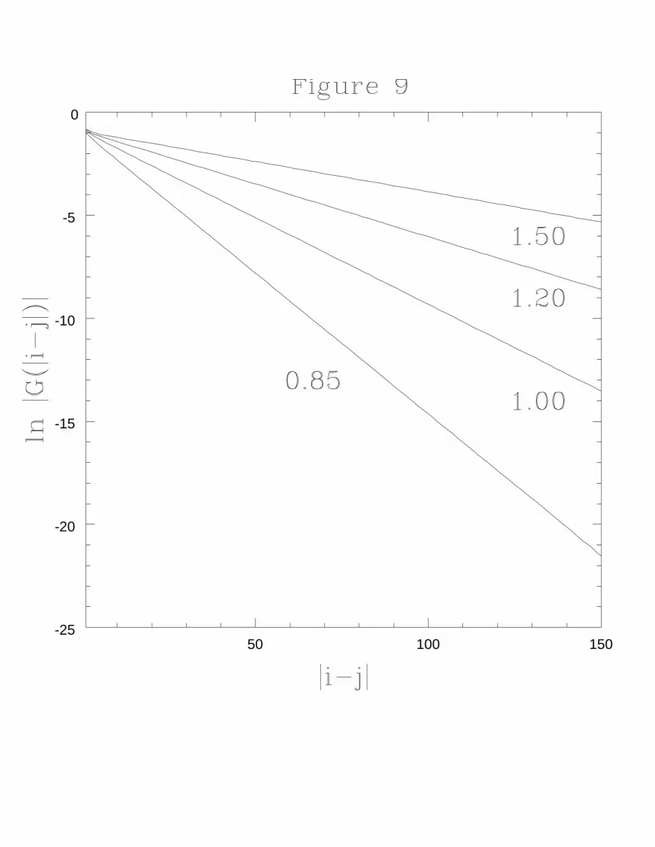
a scale much longer than the bulk correlation length for α greater than about 1 (Fig. 9). As

the Z2 × Z2 symmetry is not broken in the total chain, the string correlator is not an order

parameter, but its very slow decay shows it characterizes well the NNN-AKLT phase. The

gap increases with frustration. In the α → ∞ limit, it tends towards the unfrustrated value

∆ = 0.41050(2)α due to the chain decomposition. The correlation length first decreases; in

the large frustration limit it tends towards twice the unfrustrated value, ξ = 12.04, due to

the doubling of the lattice spacing in the decomposed chains. The bulk excitations retain

the pair structure mentioned above.

At the transition point αT = 0.7444(6) we measure the correlation length to saturate

to ξT ≈ 18 on the AKLT side of the transition, clearly excluding a critical or near-critical

point as conjectured before. We find the bulk excitation gap to be ∆T ≈ 0.10. On the

NNN-AKLT side the correlation length is longer, and might be divergent. In both phases

we can identify close to the transition edge states that are remnants of the other phase. This

together with the discontinuous jump of the string order parameter by ≈ 0.085, about 20

percent of its maximal value, leads us to classify this point as a first-order transition. This

is in accordance with the predictions of the variational approach, predicting a (too big) gap

of ∆varT = 0.325.

III. PHYSICAL SCENARIO

We now proceed to expound the physical scenario briefly outlined above. The physics

of the frustrated S = 1 quantum spin chain is entirely determined by the parameter α. We

find two phases, namely the AKLT (Haldane) and the NNN-AKLT phase, and three special

points in the phase diagram, the disorder point αD, the Lifshitz point αL and the transition

point αT .

6

A. The AKLT Phase

The point α = 0 corresponds to a nearest-neighbor Heisenberg quantum spin chain. It is

well established by now5–7 that at α = 0 the above model has a finite correlation length of

ξ = 6.03(2), a Haldane gap ∆ = 0.41050(2), and is characterized by a so-called string order

parameter24,26

Ozπ(i, j) = 〈Sz

i (expj∑

k=i+1

iπSzk)S

zj 〉 (2)

which measures the hidden order of the S = 1 Heisenberg chain, which is due to a broken

Z2 × Z2 symmetry.25 Its numerical value6 is Ozπ = lim|i−j|→∞Oz

π(i, j) = 0.374325096(2).

There is a very intuitive description of this point provided by the Affleck-Kennedy-Lieb-

Tasaki model:17,18 each S = 1 spin is decomposed into a symmetric sum of two S = 12

spins

(Fig. 1). Each of the S = 12

spins is linked to one of the neighboring S = 12

spins by a

singlet bond. The adequacy of this description is established by the fact that the AKLT

model shows the same hidden order characterized by a string order parameter24,26 Ozπ = 4

9,

has a gap to the first bulk excitation, and a finite correlation length. One of the most

striking predictions of the AKLT model verified by the Heisenberg chain is the presence of

two effectively free S = 12

spins at the right and left end of an open chain. This gives rise

to a low-lying edge excitation triplet, the so-called Kennedy triplet, which degenerates with

the ground state singlet in the thermodynamic limit.27

We argue that for αT < 0.7444(6) the AKLT model provides an adequate description and

a good starting point for a variational description of the spectrum. This is corroborated by

the observation that the string order parameter is non-zero throughout this phase (Fig. 6),

and peaks at 0.4397(1), very close to the AKLT value of 49. It drops to zero discontinuously

at the phase transition, and is thus an adequate order parameter for this phase. The results

obtained by the variational approach starting from the AKLT model are in a qualitative

agreement with the numerical findings: We observe a gap maximum at α = 0.40(1) with

∆ = 0.82(1), which is predicted at α = 0.38 with ∆var = 0.97 by the variational approach.

7

Predicted and observed gap curve are in reasonable agreement (Fig. 7). Let us however note

at this point that we do not find the intermediate drop of the gap Pati el al.15,16 observe

at α ≈ 0.5, but rather observe a monotonous drop of the gap. For a (rather technical)

explanation of the disagreement, which can be traced to the appearance of parasitical edge

states which were not taken completely into account, we refer to Section V.

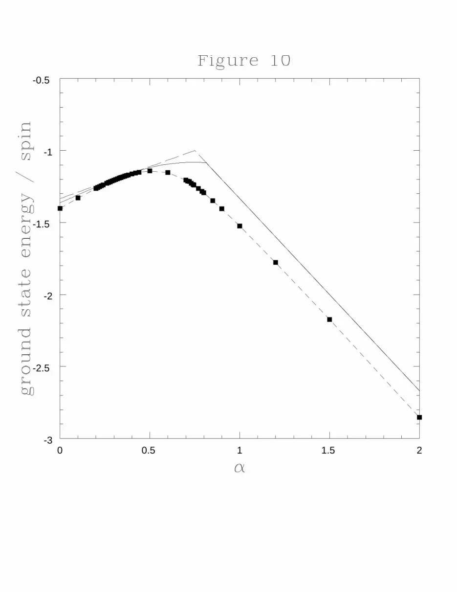
In the region where the string order parameter peaks, numerical and variational ground

state energies agree very well, and the general behavior of the ground state energy is well

predicted by the variational approach (Fig. 10).

The shift in the structure function peak away from π (explained below) is predicted

variationally at αvarL = 0.32 and found numerically at α = 0.3725(25). However, in the

variational approach the peak shifts to q = ±2π/3 as α approaches the transition point,

and then drops discontinuously to ±π/2, whereas we observe numerically that q smoothly

decreases from π to π/2 with increasing α. Here, the variational approach is too simplistic.

It is no use comparing correlation lengths: The matrix product states of the AKLT model

notoriously underestimate correlation lengths.

We conclude by remarking that we clearly observe the Kennedy triplet numerically, as a

Stotal = 1 end excitation with odd parity (abbreviated in the following as 1−), degenerating

with the 0+ ground state. The first bulk excitation is then given by the lowest 2+ state.

We have also calculated the spectrum in a chain where a spin 12

was added at each end,

binding the free spins and lifting the degeneracy.5,6 Then the ground state is given by the

lowest 0− state, and the first bulk excitation by the lowest 1+ state. The findings of both

procedures are in excellent agreement. In an open chain, there is for α > αD a low-lying 1+

edge excitation in addition to the Kennedy triplet, which we will identify as a precursor of

the NNN-AKLT phase below.

8

B. The Disorder Point in the Frustrated Spin Chain

In a previous work28 by one of us (U.Sch.) it was shown that the relationship between

the antiferromagnetic Heisenberg model and the AKLT model for S = 1 can be understood

within the framework of a disorder point of the second kind, a well-defined concept arising

in classical statistical mechanics. Let us briefly review the physical properties of such a

disorder point23,29 without mathematical details; for such details, we refer to the previous

work28 and the references cited therein.

A disorder point can arise if a system exhibits two ordered low-temperature phases

with differently broken symmetries, e.g. an antiferromagnetically ordered phase and a spiral

phase with a generally incommensurate wave number q and if these phases are linked to the

disordered high-temperature phase by continuous phase transitions. It is intuitively clear

that in the disordered phase there will be remaining short-range correlations of the type

found in the adjacent ordered phases. Moving across the phase diagram, one expects to find

a line in the disordered phase separating regions with the two different types of correlations,

a so-called disorder line. As the correlations are short-ranged, the correlation function peak

in momentum space (in S(q)) starts moving from, say, q = π to a general q not exactly

at the disorder line, but at a different line, the so-called Lifshitz line, somewhere in the

incommensurate-correlation region. The two lines join in the multicritical point, where the

two ordered phases and the disordered phase meet.

The remarkable fact is that such disorder lines, throughout a variety of substantially

different physical systems, can be classified into two types with a number of well-defined

physical properties.

Typical properties of a disorder line of the second kind (the one found here) are:

• Moving through parameter space on a path characterized by a parameter γ across

a disorder line at γ0, the correlation length ξ(γ) exhibits an infinite slope on the

commensurate side at γ0. On the incommensurate side, the slope is typically finite:

9

dξdγ

∣∣∣γ0;C

= ∞ dξdγ

∣∣∣γ0;IC

< ∞ (3)

The correlation length may, but need not have a local minimum at γ0.

• The real space correlation function changes from a commensurate to an incommensu-

rate wave number q(γ) on the disorder line. The function of the wave number q(γ)

has a singular derivative at γ0 on the incommensurate side

dqdγ

∣∣∣γ0;C

= 0 dqdγ

∣∣∣γ0;IC

= ∞ (4)

and evolves as

(q(γ) − q(γ0)) = (γ − γ0)σ (5)

for small γ − γ0.

• At γ0, there is a dimensional reduction of the real space correlation function. This

means that comparing the correlation function to an Ornstein-Zernike correlation func-

tion

〈S(0)S(x)〉 ∝ e−x/ξ/r(d−1)/2, (6)

the underlying problem seems to have a lower dimension than the original physical

problem, i.e. d < 1 + 1 here.

In the case of the frustrated antiferromagnetic Heisenberg quantum spin chain, there is

no ordered zero-temperature phase.4 However, the quantum spin chain at zero temperature

may be mapped to a classical spin chain at finite temperature. From the non-linear sigma

model30 it is known that at least for the unfrustrated Heisenberg model the temperature T

of the classical chain is linked to the quantum spin S by

T ∝ 1/S . (7)

10

The classical spin chain at finite temperatures is disordered due to the Mermin-Wagner

theorem;4 but it is ordered at T = 0. Reconsidering the arguments at the beginning of this

section, replacing temperature by inverse spin, one sees that the T = 0 classical spin chain

provides the required commensurate and incommensurate ordered low-temperature phases.

In the case of the relationship between the AKLT model and the antiferromagnetic

Heisenberg chain, one has to consider a general bilinear-biquadratic spin chain as the sim-

plest generalized Hamiltonian containing both models; it actually shows a phase transition

between an ordered commensurate and an ordered incommensurate phase in the classical

limit. The disorder point in that case, which was identified as the AKLT model,28 is thus a

quantum remnant of the classical phase transition.

For a classical frustrated antiferromagnetic Heisenberg chain, there is a similar phase

transition. For α < αc = 0.25, the chain is antiferromagnetically ordered:

〈S0Sx〉 ∝ cos qx (8)

with q = π. For α > αc, there is spiral order

〈S0Sx〉 ∝ cos q(α)x (9)

with

q(α) = arccos(−1/4α). (10)

In analogy to the bilinear-biquadratic spin chain, we may therefore predict the presence of

a disorder point for a certain αD, exhibiting the same properties as listed above. Indeed,

we can identify an αD = 0.284(1), which meets the above criteria to numerical precision.

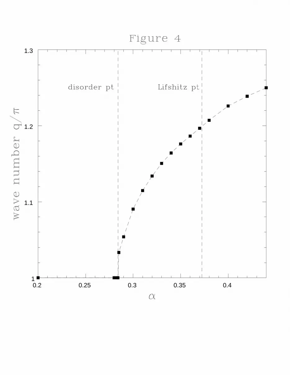
Correlations become incommensurate in real space at this point (see Fig. 2). The wave

number q for α > αD (Fig. 4) obtained from fits to a two-dimensional Ornstein-Zernike

correlation function

〈S0Sx〉 ∝ cos q(α)xexp(−x/ξ(α))√

x(11)

11

shows the expected singular behavior; the singularity is roughly square-root-like. Figure 3

shows a minimum of ξ ≈ 1.20 at this point, and a very steep slope of ξ for α < αD. It

is numerically not infinite but clearly much bigger than the slope on the incommensurate

side. We are not able to show the dimensional reduction at the disorder point numerically;

at very small correlation lengths, it is hard to distinguish between purely exponential and

mixed exponential-power law behavior. At the disorder point, it seems easier to obtain a

purely exponential fit to the correlation function; but the data does not seem precise enough

that we would want to make a definite statement here.

In the case of the AKLT disorder point this identification was easily possible due to the

analytically known properties of its ground state. As all other data ties in extremely well

into a very plausible physical scenario, we are convinced that our identification is correct.

For 0.37 < α < 0.375 we find the associated Lifshitz point, where the S(q) structure

function develops a two-peak structure (see Fig. 5). There is no particular behavior of

the structure function at the disorder point apart from a maximal broadening due to the

minimum in ξ. This point has already been found by Pati et al.15,16 to be at 0.39(1). As

we have investigated longer chains at higher precision, we consider our result to be more

precise. In any case, this minor disagreement has no direct physical implications.

The particular feature of the Lifshitz point is the development of a doubly-degenerate

structure of the excitation spectrum. Let us remark that the existence of two fundamentally

different spectra has already been predicted by Allen and Senechal;14 they had numerical

data suggesting that spectra switch at α ≈ 0.4.

Let us consider closed chains (all statements in the following are for chains of even

length). In the AKLT phase, a closed chain can be simulated numerically by adding a spin

12

at each chain end, as long as the energy to excite the bonds of these spins to the chain

exceeds the bulk gap energy. We find numerically for this modified chain:

• α < αL: The ground state is given by the lowest 0− state. The first bulk excitation is

given by the lowest 1+ state, which does not degenerate with the lowest 1− state.

12

• α > αL: At the Lifshitz point, the lowest 1+ state degenerates with the lowest 1−

state, which was higher in energy in the single-state spectrum. This corresponds to the

double peak structure evolving in S(q): classically speaking, the two degenerate states

correspond to spin waves cos qx (even parity) and sin qx (odd parity). The ground

state is still given by the lowest 0− state.

These observations can be reproduced in unmodified open chains, if edge excitations are

excluded from the spectrum (see Figs. 12 and 13, discussion in Section V).

Let us briefly discuss the behavior of the gap and the string order parameter. As can

be seen from figures 7 and 6, the maximum of neither is associated with one of the two

special points just discussed. This is no surprise in the case of the gap, which has no

particular relationship to the disorder point phenomenon. The maximum of the string order

parameter lies at 0.33 < α < 0.335, clearly separated from the disorder point. In our

previous study28 we found the maximum of the string order parameter to be at the disorder

point. This was however a particular feature due to the identification of the AKLT point

as the disorder point in the bilinear-biquadratic S = 1 spin chain. As the string order

parameter is particularly adapted to the AKLT model, it showed its maximum there. In

our present study, the disorder point need not be (and obviously is not) associated with the

frustrated Hamiltonian “closest” to the AKLT model in a generalized coupling space.

C. The Next-Nearest Neighbor AKLT Phase

In the limiting case α = ∞, the frustrated chain decomposes into two unfrustrated

chains on the even and odd sites. Each of these chains can be adequately described by

the conventional AKLT model. We thus use the next-nearest neighbor AKLT model as

shown in Fig. 1 as starting point for our argumentation. Observe that in an open chain,

there are two free S = 12

spins at each chain end, which we link up by nearest-neighbor

singlet bonds. There are therefore no free end spins, and the ground state of an open

chain is not degenerate. This can be verified numerically. The low-lying bulk excitation

13

spectrum retains its doubly-degenerate structure. The ground state energy per site should

asymptotically behave as E0(0)α, where E0(0) is the ground state energy of the unfrustrated

chain. Fig. 10 shows that the asymptotic behavior is already reached for intermediate α,

lending support to our variational ansatz. We expect an excitation gap of ∆(α) = ∆(0)α in

the α → ∞ limit. Our numerical calculations (Fig. 7) show that the asymptotic behavior of

the gap is already approached for intermediate α, lending further support to the variational

ansatz. The observed gap exceeds the asymptotically expected gap, as it costs more energy

to excite a chain which is still (weakly) linked to the other one.

In the limit of very strong frustration, we expect also a correlation length which is

twice the unfrustrated correlation length, due to the doubling of the lattice spacing: ξ(α →

∞) = 12.04. For the correlation length we observe numerically a drop away from the

transition point to a plateau of ξ ≈ 10 at α ≈ 2, with an increase of ξ for larger α. The

correlation length is smaller than asymptotically expected, corresponding to the too large

gap. We cannot make any statement on the large-α behavior, as the DMRG precision

becomes insufficient.

Let us now address the question whether there is an order parameter characterizing this

phase in analogy to the conventional string order parameter in the AKLT phase. Consid-

ering the next-nearest neighbor AKLT model, the natural generalization of the string order

parameter is given by

Gzπ(i, j) = 〈Sz

i (expk≤j∑

k=i+2,...

iπSzk)S

zj 〉, (12)

where i and j are both even (odd), i.e. on the same subchain. At least for α = ∞, this must

be a good order parameter.

We observe numerically that G vanishes in the AKLT phase with a decay length sub-

stantially shorter than the spin-spin correlation length. In the NNN-AKLT phase it does

not exhibit a finite value for |i − j| → ∞ (consider Fig. 9). The decay can be very well

fitted to an exponential; a power-law decay is excluded for the values we have considered.

In contrast to the conventional string order parameter, our generalization is thus not an

14

order parameter. However, it does characterize the nature of this phase in accordance with

our analytical model: above α ≈ 1, the decay lengths are typically much longer than the

associated spin-spin correlation lengths: for α = 2, the ratio is already of the order of 10. We

argue that the difference to the Haldane phase is given by the restoration of the Z2×Z2 sym-

metry on the chain, as characterized by the disappearance of the conventional string order

parameter. In the AKLT picture this is graphically represented by the two nearest-neighbor

singlet bonds at the chain ends. In the finite frustration case, we characterize the symmetry

on each subchain as “almost” broken: obviously it is broken on the isolated subchains; but

the coupling between the subchains (weaker with increasing α) restores the symmetry on a

length scale much longer than the system correlation length. The following simple picture

can help to illustrate this phenomenon physically: the difference between our AKLT phase

and the exact AKLT state is that in the AKLT phase there exist bound pairs of solitons

in the hidden (string) order, and the same applies to the subchains in our NNN-AKLT

phase, but now there is a nonzero probability of having a bound pair with solitons sitting

on different subchains, which destroys the long-range string order inside subchains on the

scale which is roughly the mean distance between soliton pairs. For the Heisenberg point,

variational studies31 indicate that this mean distance is about 60 lattice sites. However, we

have no argument at the moment concerning the α dependence of this length scale. Further

work is necessary to fully understand this phenomenon.

D. The First Order Phase Transition at α = 0.7444(6)

The remaining question is how the change from the AKLT to the NNN-AKLT phase at

α = 0.7444(6) can be characterized. Basically, we have to decide between (i) no transition,

but a gradual change; (ii) a first-order phase transition; (iii) a continuous phase transition.

Let us recall that in the related bilinear-biquadratic S = 1 quantum spin chain there is a

continuous phase transition on the incommensurate side of the disorder point at the Lai-

Sutherland point.32,33 In the following, we want to discuss our numerical and analytical

15

evidence which definitely excludes a critical point and thus a continuous phase transition,

and clearly indicates a first-order transition. Let us first present the raw data.

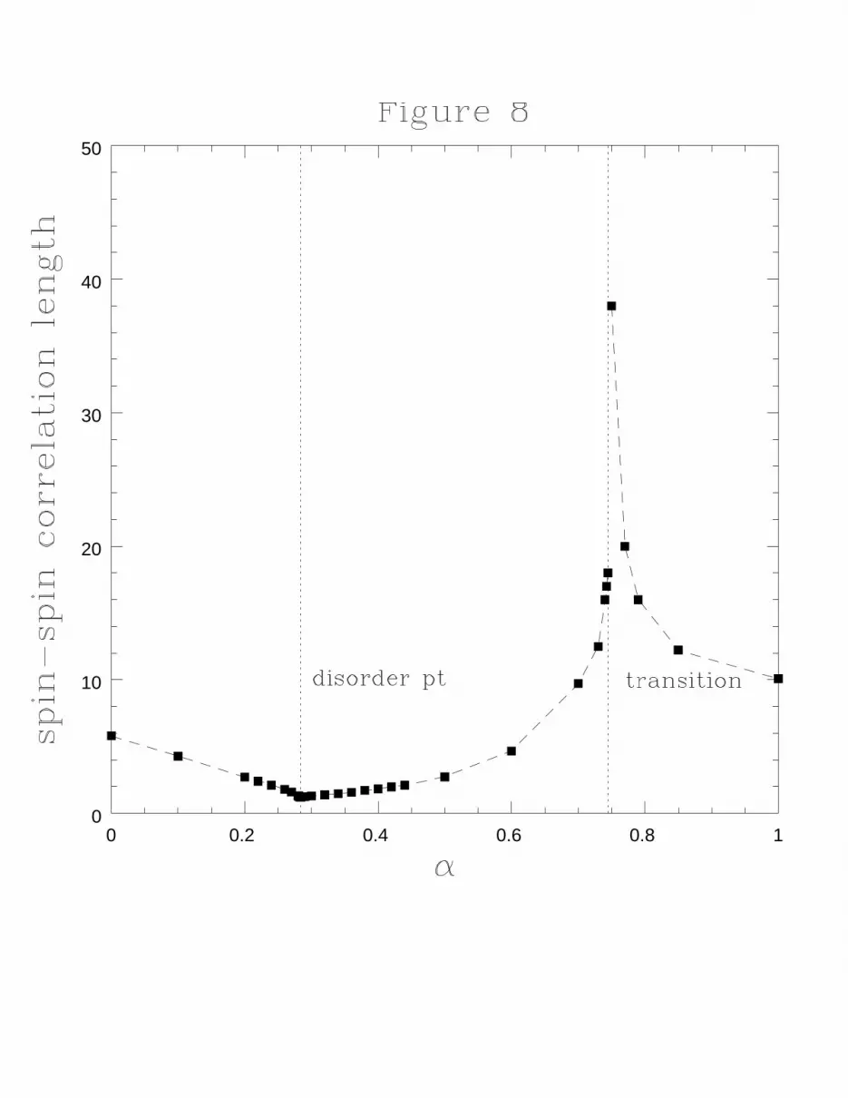
In the AKLT phase below the transition, we observe a finite correlation length peaking

at the transition with a value of ξ ≈ 18 (see Fig. 8). This data, obtained from chains of

L ≤ 380, clearly excludes a continuous phase transition, which would require a divergent

correlation length on both sides of the transition. In the NNN-AKLT phase, the correlation

length is much longer. Immediately above the transition, our numerical data does not allow

the extraction of a reasonable correlation length. We can thus not decide whether it is

finite or divergent at the transition in the NNN-AKLT phase. This behavior corresponds

to a pronounced peak in the structure function, but there is no particular behavior of the

peak location q. Apart from the exclusion of a continuous phase transition, the apparent

discontinuity in the correlation length strongly suggests a first order transition.

We observe a finite gap ∆(α) (Fig. 7) everywhere in the same range. This fact is obscured

by the presence of parasitic low-lying states corresponding to edge excitations, as explained

in Section V. The minimal gap is rather small, ∆ ≈ 0.10, to be compared with a variational

prediction of ∆ = 0.325. At the transition, the precision of the gap is not too high; estimates

we give are at the lower bound. In the AKLT phase, the observation of a finite gap ties in

with the observation of a finite correlation length. The case of the NNN-AKLT phase we

will discuss below.

Our main argument in favor of the first order transition is the clearly discontinuous

disappearance of the string order parameter (Fig. 6). We observe numerically a jump of

0.085 (20 percent of its maximum value) between α = 0.74375 and α = 0.74500. Up to α =

0.74375, the string order parameter decays almost linearly; at this point the slope increases

about sixtyfold. We think it is therefore extremely unlikely that there is a crossover from

this linear behavior to an extremely strong power-law decay (as in a continuous transition),

but identify this behavior as a discontinuous jump.

A first-order transition would be most neatly identified by a discontinuous derivative of

the ground state energy per spin. Numerically, we find it very difficult to clearly identify

16

such a discontinuity. Though the correlation length is finite at least in the AKLT phase,

it is long enough to suggest a rather soft first-order transition. The presence of degenerate

edge states at the transition further obscures the numerical data.

Another characteristic feature of a first-order transition is the so-called level crossing: at

the transition, the energy of one of the two ground states involved drops below the other

one. Typically, certain wave function symmetries change at the transition, and close to the

transition, in each phase there should be a trace of the ground state of the other phase.

Considering the non-local order parameter, one may not expect that the symmetry changed

is revealed in a change of parity or the total spin of the ground state, two quantities we

control. Actually, the ground state is 0+ in both phases. But its degeneracy changes from

4 (AKLT) to 1 (NNN-AKLT), indicating the change of some more complex wave function

symmetry.

We propose the following physical scenario at the transition, which is strongly supported

by our numerical data, and which gives a mechanism for the first-order transition:

• Below the transition, in the AKLT phase, we find a 1+ edge excitation (see Section V,

Figs. 12 and 13), which degenerates with the ground state at the transition. This edge

excitation is a precursor state of the transition: In the 0+, 1− and 1+ state we observe

that the center of the chain is characterized by an exponential decay of correlations.

We say it is in the bulk phase, which is just the AKLT phase. Close to the transition

the chain ends, however, belong to a different edge phase: as we calculate spin-spin

correlations symmetrized around the center, this is evidenced by a clear change in

the spin-spin correlation function. For longer chains at fixed α, we find that the bulk

region grows, but not the edge region, showing that we are in fact dealing with an

end effect. We call this a pseudo coexistence of phases: though they coexist on the

finite chain, the edge phase is not extensive; in the thermodynamical limit it is just a

boundary effect, so there is no true coexistence. We may however consider the chain

ends as a nucleation center for the new phase: we suppose this is because the open

17

chain ends allow a lowering of energy by replacing an AKLT chain with free end spins

by two chains, whose free end spins can be bound by singlets, which lower the energy.

We identify the edge phase with the NNN-AKLT phase, because its influence exists

only close to the transition and the string order parameter does not develop a finite

long-range value in the edge phase. At the transition the AKLT bulk phase, whose

correlation length is finite all the way, is pushed out entirely, as the NNN-AKLT edge

phase becomes extensive. At this point, the 0+, 1+ and 1− states are degenerate (to

numerical precision). The bulk excitation of the AKLT phase has a finite gap up to

the transition.

• Above the transition, in the NNN-AKLT phase, there is no bulk-edge separation in

the ground state. There is a low-lying 1± pair of states (almost) degenerate with the

ground state at the transition, emerging as low-lying excitations. The magnetization

is concentrated in the chain ends, shifting towards the center, as the energy cost of this

excitation approaches that of a NNN-AKLT bulk excitation. Calculating increasing

chain lengths for fixed α, the magnetization remains at the chain ends. These exci-

tations must thus be classified as edge excitations, until the gap between 1± and 0+

becomes of the order of the bulk gap between 2± and 1±. We observe the following

interesting phenomenon: Up to the discontinuous jump, the string order parameters

as calculated in the 0+ and the 1± states agree to numerical precision, excluding the

edge regions. After the transition, the string order decays fast to zero in the 0+ ground

state, but remains non-zero in the bulk of the 1± states much longer before decay-

ing. With increasing α (as the excitation wanders into the bulk) the decay behaviour

aproaches that of the 0+ state, and the string order starts fluctuating strongly. The

effect disappears at α ≈ 0.80. The correlation length observed in the center region ties

in well with the AKLT correlation length just below the transition.

We suggest, on the above grounds, that those 1± states are the trace of the old AKLT

ground state in the new phase, however, “polluted” by parasitic edge excitations.

18

Then, the described spectrum behavior is consistent with the level crossing picture

and with all the other data indicating the first order transition. Assuming that the

spin wave velocity does not diverge at the transition, our gap curve would suggest that

the correlation length is finite on the NNN-AKLT side of the transition also.

We are therefore led to locate a first-order phase transition at αT = 0.7444(6), in very

good agreement with the naive analytical prediction αvarT = 0.75 (see next section).

In the following we discuss in more detail our variational and numerical approaches.

IV. ANALYTICAL RESULTS: VARIATIONAL APPROACH TO THE

FRUSTRATED SPIN CHAIN

In the following we are presenting our variational calculations. Such calculations are

very useful to understand the nature of the ground state and the excitations of quantum

systems, and even get a quantitative estimate of energies. However, strictly speaking, no

variational result can be considered a strong argument, as far as the nature or very exis-

tence of a phase transition is concerned. Nevertheless, in many cases a variational study

of the ground state and the elementary excitations, while looking for the possible points

where the gap closes, turns out to be useful and gives an important hint of the actual sys-

tem behavior. For example, variational studies of the solitonic excitations in the S = 1

chain20,34–36 allow one to reproduce qualitatively the structure of the phase diagram in the

presence of anisotropies, biquadratic exchange, and an external magnetic field; a variational

study of the Shastry-Sutherland-type37 solitons in the dimer order qualitatively captures the

picture of the transition from the dimerized to the nondimerized phase.38 Therefore we will

present here the variational results for frustrated S=1 chain as arguments complementing

the numeric findings. The good agreement between the physical assumptions underlying

the variational ansatz and the numerical results shows that we capture essential parts of the

physics of the frustrated S = 1 chain.

19

A. Ground State and Elementary Excitations: A Naive Approach

In the most naive way, one can attempt to describe the ground state of the frustrated

S = 1 chain as being the AKLT state below an αvarT and NNN-AKLT state above. The

ground state energy per spin E0 then would be EAKLT0 = −4/3 + 4α/9 in the AKLT phase

and ENNN0 = −4α/3 in the NNN-AKLT phase, which gives a rough (but surprisingly good,

see Fig. 10) estimate for the transition point αvarT = 3

4.

The elementary excitations in the AKLT phase then can be studied in a soliton approach

in the spirit of Refs. 19,20. Technically this is most easily done in the matrix product states

formalism.39,40 Let us briefly summarize the results. The AKLT state can be represented in

the form of a trace over the matrix product

|AKLT 〉 = Tr(N∏

i=1

gi) , (13)

where

gi =1√3

|0〉i −√

2|+〉i√

2|−〉i −|0〉i

(14)

is a 2×2 matrix composed of the spin states of the i-th site. The soliton (“crackion,” in

the terminology of Fath and Solyom) state |Cµn〉, describing the soliton in the string order

located at the n-th site and having Sz = µ, µ = 0,±1, can be written as

|Cµn〉 = Tr(

n−1∏

i=1

gi(σµgn)

N∏

i=n+1

gi) , (15)

where σµ denotes the Pauli matrices in the spherical basis. Physical excitations with a

definite momentum can be easily constructed as |Cµ(k)〉 =∑

n eikn|Cµn〉, and their dispersion

is

εµ(k) =〈Cµ(k)|(H − E0)|Cµ(k)〉

〈Cµ(k)|Cµ(k)〉 .

The averages can be calculated using the transfer matrix technique (see Refs. 40,41), and

finally, after a simple but lengthy calculation, one arrives at the following formula for the

dispersion law of the soliton excitation at α < 0.75:

20

εµ(k) =14

9+

26

27α +

160α − 18

27cos(k) − 14

9α cos(2k)

+ (2 − 26α/3)3 + 5 cos(k)

5 + 3 cos(k)(16)

Because of the isotropy of the problem, all three branches with different µ are degenerate.

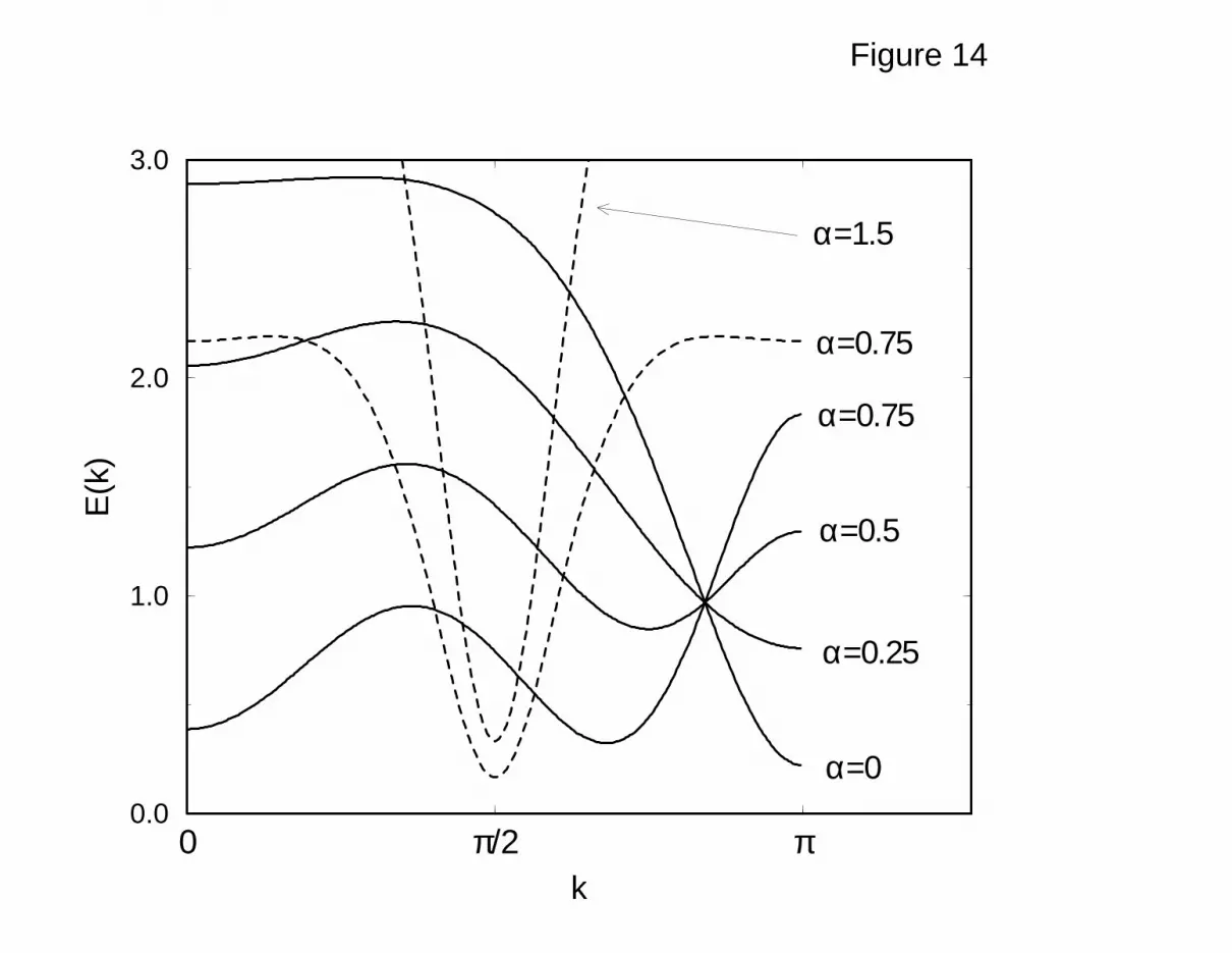
A few typical dispersion curves at different values of α are displayed in Fig. 14. One can

see that above some critical α = αvarL ≃ 0.32, the minimum of the excitation energy is found

for a momentum k = q0 6= π, and q0 tends to 2π/3 as α tends to αvarT = 3

4(see Fig. 11).

One may speculate this point αvarL can be identified with the Lifshitz point, though in fact

there are no incommensurate correlations in the AKLT state. Note that in the numerical

calculations the lowest excitation becomes doubly degenerate when α crosses the Lifshitz

point. This can be easily explained14 by the fact that the two minima of the dispersion

curve at k = ±q0 are physically inequivalent if q0 6= 0, π.

The gap does not disappear at the transition point (∆var(α = 0.75) ≃ 0.325), indicating

a first-order phase transition (or absence of a phase transition). The α dependencies of

the gap ∆var and of the wavevector qvar0 with minimal excitation energy obtained from this

simple calculation qualitatively agree with the numerical data (see Figs. 7 and 11).

On the other side of the transition point we take the NNN-AKLT state (Fig. 1) as a

variational ground state, and the soliton dispersion in the thermodynamic limit L → ∞

(when the chains become decomposed in the NNN-AKLT picture) can be obtained from

(16) by first setting α to zero, replacing k → 2k, and finally scaling the whole expression by

α; this gives for α > 0.75 the gap Eg = 2α/9 (similarly to Eg = 2/9 at the Heisenberg point

α = 0) and q0 = π/2 as wavevector with minimal excitation energy. Actually, as it follows

from the numerics, Eg(α) → αEg(0) only asymptotically at α → ∞, but one can also see

from the numerical data that this asymptotic linear behavior above α = 0.75 sets in rather

quickly.

21

B. 4× 4 Matrix Product Variational Ansatz

The “purely AKLT” description presented above is of course not very satisfactory: in

fact, we did not even have any variational parameters and simply compared two VBS con-

figurations being intuitively good candidates for the ground state. However, it is easy to see

that those two choices are not the only possible ones: for example, at α = 0.75 the energy

per spin of the completely dimerized valence bond state is exactly the same as that of the

AKLT and NNN-AKLT configurations. One thus may try to consider some more general

variational wavefunction capable of interpolating between different VBS states.

We have found that such wavefunctions can be constructed in the matrix product states

formalism, at the price of going to a higher matrix dimension and considering larger clusters.

One possible simplest choice for the elementary matrix is

Γ12 =∑

ij

|t1it2j〉 Aδij(11 ⊗ 11) + iBεijk(σk ⊗ 11)

+ iC(σi ⊗ σj) , (17)

where the matrix state Γ12 lives on a cell consisting of two adjacent spins 1 and 2. σi,

i = x, y, z are the usual Pauli matrices (in the cartesian basis), 11 denotes the 2×2 identity

matrix, and |ti〉 denotes the triplet of spin-1 states in the cartesian basis:

|tx〉 = −(1/√

2)(|+〉 − |−〉) ,

|ty〉 = (i/√

2)(|+〉 + |−〉) ,

|tz〉 = |0〉 .

Since both the Pauli matrices and the triplet wavefunctions |ti〉 behave as vectors under

rotations, the matrix (17) behaves as a scalar. Therefore, the matrix product state

|Ω〉 = Tr (∏

l

Γ2l−1,2l) , (18)

constructed from such elementary matrices, obeys the rotational invariance of the problem

(note that the usual AKLT matrix (14) is unitary equivalent to (1/√

3)∑

σi|ti〉, and this

22

is the only possible rotationally invariant ansatz if the dimension is 2×2 and the matrix

lives at one site, but in higher dimensions and for larger cluster sizes the number of choices

rapidly increases).

The wavefunction (18) has the remarkable property that it interpolates smoothly between

the AKLT state (A = B = 1/3, C = 0), the completely dimerized state (A = 1/√

3,

B = C = 0), and the NNN-AKLT state (A = B = 0, C = 1/3).

The quantum averages can be calculated in the usual way; however, the complexity of

solving the analytic eigenvalue problem for the 16×16 transfer matrix G = Γ∗12Γ12 forced

us to restrict ourselves to the case of real coefficients A, B, C. Then, setting the largest

eigenvalue of G to 1, one obtains the normalization condition

3(A2 + 2B2 + 3C2) = 1 (19)

which leaves us with two independent real variational parameters. The variational expression

for the ground state energy per spin

Evar = −4α/3 + 4B2(4α − 3) − 3(A2 − B2) (20)

+ 2(A − B)2A3 + 10A2B + AB2 − 2A/3

+ 5B3 − 10B/3 + α[ − 10A3 − 10A2B

−2AB2 + 16(A + B)/3 − 2B3]

can be minimized numerically; the resulting dependence of the ground state energy on α is

presented in Fig. 10. The main feature is that though the discontinuity at the transition

is less distinct than in the “naive” picture, and the transition point shifted towards larger

α ≃ 0.81, the transition still is found to be first order. At the Heisenberg point α = 0

the variational result for the ground state energy is Eminvar = −1.364, being slightly better

than the AKLT value −43. However, the disadvantage of the ansatz (18) is that it explicitly

breaks the translational invariance, and thus the ground state has a built-in dimerization

which is always nonzero.

23

The lowest excitations above this variational ground state can be calculated using the

single-mode approximation in the spirit of Arovas et al.42 Since we have now two spins

involved in the elementary matrix (17), it is natural to write down the wavefunction of the

excited state in the form |Cµ(k)〉 =∑

n eikn|Cµn〉, where

|Cµn〉 = Tr(

n−1∏

l=1

Γ2l−1,2l · ΓµC ·

N∏

l=n+1

Γ2l−1,2l) , (21)

ΓµC = (Sµ

2n−1 + λ(k) · Sµ2n)Γ2n−1,2n .

Here Sµl denote the components of the spin-1 operator at the l-th site, λ is an additional

(complex) variational parameter whose value has to be determined numerically for each

value of the wavevector k, and k now varies from 0 to π/2 since the elementary cell is

doubled. The resulting gap dependence on α is shown in Fig. 7. One can see that there

is a local minimum around α = 0.75, but the gap in the transition region is considerably

overestimated, even comparing to the naive approach described in the previous subsection;

we attribute this fact to the built-in breaking of the translational invariance in the ansatz

(18) as explained above.

V. NUMERICAL RESULTS: DENSITY MATRIX RENORMALIZATION GROUP

CALCULATIONS

A. General Remarks

Using the Density Matrix Renormalization Group (DMRG), we have calculated for this

problem (i) the gap between the ground state and the lowest excitation, (ii) the magnetiza-

tion for the lowest excited state, (iii) the string order parameter O and the string correlator

G and (iv) the spin-spin correlation function. For details on the DMRG we refer to the

literature.5,21 The DMRG is particularly suited for the problem under study as it is not

limited to small systems like exact diagonalization and as it is not plagued by the negative

sign problem which Quantum Monte Carlo typically encounters in frustrated systems at

very low temperatures.

24

For our calculations, we have studied chains of a length up to L = 380 and typically

kept M = 250 block states in each iteration. To reduce both memory usage and improve

program execution speed, we have used the following DMRG features:

• We have used both the total magnetization and left-right parity as good quantum

numbers. This reduces storage, but also thins out the Hilbert space, giving faster

convergence of the implemented exact diagonalization, and allows for fast classification

of the spectrum.

• We have implemented a prediction algorithm which gives a guess for the eigenstates of

a DMRG step based on the eigenstates of the preceding DMRG step. This algorithm,22

similar in spirit to the one introduced recently by White,10,43 allows for a substantial

reduction of the number of iterations needed in the exact diagonalization, truncating

it by a factor of up to 10. It should however be mentioned that the speed-up due

to the prediction algorithm is biggest when the studied system has a rather short

correlation length; so its use is somewhat limited there where most performance would

be needed. A further problem is that it does not cut the time needed for the calculation

of expectation values, a dominant feature of our calculations.

It is important to realize that (unlike in exact diagonalization studies) it is not sufficient

to extrapolate results to the thermodynamic limit in L only. The performance of the DMRG

depends crucially on the number M of block states kept; as a rule of thumb, the number

of states M to be kept increases dramatically close to critical points or phase transitions,

which reflects the increasing number of low-energy fluctuations or competing states. The

precision of the DMRG is indicated by the truncation error, which allows for extrapolations

to the exact M = ∞ result. Let us remark that good agreement between DMRG and exact

diagonalization results for a given M is not necessarily an indicator of good DMRG precision:

exactly diagonalizable systems are notoriously small, and our results indicate that DMRG

errors build up severely with system length.

We found that close to the disorder and Lifshitz points (a region where the ground state

25

should have a relatively simple valence bond structure) M = 80 is sufficient to give highly

precise results; near the phase transition, convergence up to M = 200 was poor, forcing us

to go up to M = 250 states. It was not possible to go to the limit of very high α: in this

case, the chain essentially decouples into two subchains, leading to a ground state which

can be understood as a product state of the ground states of two unfrustrated chains. The

description of such a product state implies a dramatic increase in M , as already observed

in other works.10,44

The numerical investigation of the phase transition was further complicated by the fact

that the DMRG works best for open boundary conditions. At the transition point it was

therefore not possible to use periodic boundary conditions, as the precision obtained for

open ones was already only moderate. Open boundary conditions may however introduce

additional edge states into the spectrum which suggest often radically different physical

properties. A good example is provided by the unfrustrated open integer spin chain with

spin S, where there are two effectively free S/2 spins at each chain end. For the S = 1

chain these free spins introduce the well-known Kennedy triplet, which degenerates with the

ground state. One therefore has the fifth state as the first bulk excitation. In the frustrated

chain, the situation will be shown to be not always as clear. To identify the lowest bulk

excitation, it is therefore necessary to calculate 〈Szi 〉 for all low-lying states. Edge excitations

due to the open chain ends can be identified by very small 〈Szi 〉 in the chain center and big

〈Szi 〉 at the chain ends and thus excluded.

B. Calculation of Correlations

For α < αD spin-spin correlation lengths can be obtained by a fit of the spin-spin cor-

relations to a law (−1)x exp(−x/ξ)/√

x, which is in all cases extremely well obeyed, except

exactly at the disorder point. Note that all DMRG correlation lengths are underestima-

tions of the true correlation length. For the longest correlation length in that region (at

α = 0), we obtain ξ ≈ 5.8, underestimating the true result by about 3 percent. As the

26

correlation length decreases as well as the truncation error with α (it is essentially 0 at

the disorder point), the error diminishes. The correlation length at the disorder point we

estimate to be precise to the order of 1 percent or better. All other correlation lengths lie

in between. For α > αD, correlation lengths are obtained by a least square fit of the data

to a law cos qx exp(−x/ξ)/√

x, with q and ξ to be determined. Extremely good such fits

could be obtained. Alternatively, one may simply plot |〈SiSj〉|√|i − j| logarithmically. As

the logarithm is not very sensitive close to correlation function maxima, simply drawing an

upper straight-line envelope gives a very simple estimate which is hardly worse despite the

incommensurate correlations. Again, the correlations obtained in that way are underesti-

mated. Considering the results for various M we claim that we underestimate at worst by

about 20 percent around the transition; at the transition itself, the data is inconclusive on

the NNN-AKLT side. Just below the transition, edge effects become strong, and have to be

excluded from the calculation of the correlation length. In short chains, the bulk behaviour

may not be visible. Edge effects can be identified by calculating longer chains: the region

of bulk behavior extends with L.

The string order parameter is a quantity particularly suited for treatment by the DMRG:

It reaches its thermodynamical limit very fast; the decay to the thermodynamical limit is on

a scale of the order of half the bulk spin-spin correlation length, as was already observed for

unfrustrated spin chains.21 Its convergence to its exact value in M is also very fast, unlike

the convergence of the correlation length.

C. Gap Calculations: The Spectrum of Open Chains

The calculation of the bulk excitation gap was the most difficult calculation performed,

because of the already mentioned problem of edge excitations inherent to open chains as

used by the DMRG. Ground state and lowest excited state energies were first extrapolated

in M for fixed L (using the roughly linear dependence of the error in energies on the DMRG

truncation error) and then extrapolated in L using quadratic convergence laws, which are

27

very well verified. This allows us to obtain gaps with a precision up to 10−3, at least 0.02

at the transition. The essential difficulty arises from the correct identification of the lowest

bulk excitation. For most values of frustration, this can be nicely done by calculating the

〈Szi 〉 distribution along the chain for Sz

total = Stotal (see Fig. 12). Typically, it is very easy to

distinguish true bulk excitations from edge excitations. To devise a more stringent criterion,

it is useful to study the rather rich behavior of the low-energy excitation spectrum of open

frustrated chains, as the DMRG deals best with open systems. In fact, though the open chain

spectrum is more complicated, the mechanism of the phase transition is better revealed here,

as the associated symmetry breaking is obvious in the presence or absence of effectively free

end spins. We find the following scenario (all statements for chains of even length; example

spectra are given in Fig. 13; the arrow indicates the gap energy):

• α < αD: The ground state is given by the lowest 0+ state: there is an odd number of

singlet bonds in the bulk, the two effectively free end spins are linked by an extremely

weak singlet bond, giving a total even number of singlet bonds. Exciting this weak

singlet bond gives a 1− triplet excitation, degenerating with the ground state (the

Kennedy triplet). The first bulk excitation is given by the 2+ quintuplet excitation,

combining a bulk and an edge excitation. The 2− quintuplet is not degenerate with

the 2+ quintuplet, and can be identified as an edge excitation.

• αD < α < αL: The open boundary conditions introduce a further parasitic edge

excitation 1+: this edge excitation we identify from its evolution with α as a precursor

of the phase transition and the NNN-AKLT phase. Even parity coupling of edge spins

is energetically disfavored in the AKLT phase, 1+ lies much higher than 1−.

• αL < α < αT : As already described for the closed chain, the bulk excitations degenerate

in pairs of odd and even parity excitations with identical total spin. The ground state

is still the same 0+ state, there is a degenerate Kennedy triplet 1−. The lowest bulk

excitations are now given by the degenerate 2± quintuplet excitation, combining a

1± bulk excitation with a 1− edge excitation (see Fig. 12). The 1+ edge excitation

28

lowers its energy with α, degenerating with the ground state at αT . For numerical

calculations it is important to realize that there may be two S = 1 excitations below

the true bulk excitation. Following the gap calculation procedure described by Pati et

al.,16 we can explain the difference between their and our gap curve for α ≈ 0.5 arguing

that they have measured the energy difference between the two edge excitations. The

numbers we obtain that way agree perfectly with theirs. As the 1+ edge excitation

degenerates with the 1− excitation at the transition, a vanishing gap is suggested, as

reported in their work. This is however not the true bulk excitation.

• α = αT : For the behavior of the spectrum at the transition, we refer to Section III D.

• α > αT : Beyond the transition, the ground state 0+ is unique, as the Kennedy

triplet disappears. The situation is basically not very complicated for the lowest bulk

excitation: there is a doubly degenerate 1± bulk excitation as below the transition.

The actual location of this state in the complete spectrum of the open chain however

varies: just above the transition, there are low-lying 1± edge excitations. The bulk

excitation is hidden in the lowest 2± state. For intermediate and strong frustration, the

chain decouples effectively into two subchains which are only weakly interacting: The

nearest-neighbor singlet bonds at the chain ends become increasingly easy to excite

for increasing α, giving four free spins-12. These couple into 16 states degenerating for

α → ∞, coupling into one 0+, two 1−, one 1+ and one 2+ state. The bulk gap, on

the other hand, scales with α. As soon as edge excitation energies drop below the bulk

gap energy, the bulk excitation will only be present in higher spin states, which have

to be identified by the magnetisation. Numerically, one can keep the bulk excitation

in the 1± state by increasing the interaction strengths at the chain ends, to disfavor

edge excitations.

We have calculated the lowest energy-states in the following sectors of the Hilbert space:

0+, 1+, 1−, 2+ and 2−, to verify the above scenario by considering the bulk magnetiza-

29

tion. For sufficiently long chains, it was always possible to clearly separate bulk from edge

excitations as in the above scenario.

VI. CONCLUSION

The numerical results presented above together with the variational calculations allow

to devise a clear and coherent picture of the behavior of a frustrated S = 1 isotropic

Heisenberg spin chain. Its behavior is fundamentally governed by the underlying classical

model, which is characterized by a phase transition from an antiferromagnetic to a spiral

ordered phase. On the other hand, pure quantum effects are prominent. As predicted from

the non-linear sigma model, the system is gapped for all values of frustration. However,

there are two clearly separated phases present. The first one for small frustrations can be

well understood in terms of the Affleck-Kennedy-Lieb-Tasaki model and is characterized

by a non-vanishing conventional string order parameter. The classical phase transition

is reflected by the presence of a so-called disorder point, where the spin-spin correlations

become incommensurate. The classical phase transition is thus not linked to the first order

phase transition found for larger frustration. The disorder point is clearly related to the

disorder point in a bilinear-biquadratic quantum spin chain, which is exactly the AKLT

model. The phase transition found at α = 0.7444(6) is purely quantal in character. It

is first order, characterized by a non-vanishing gap and a finite correlation length on the

AKLT side. We observe a non-continuous change both in the string order parameter and in

the correlation length. The Z2 × Z2 symmetry broken in the AKLT phase is thus restored.

A string correlator which considers only every second spin characterizes this phase. We

also suggest that if one includes the alternation of [1 + (−1)iδ] type in the nearest-neighbor

interaction in the Hamiltonian (1), there will be a first-order transition line in the (αδ) plane.

Assuming that the transition line is characterized by vanishing string order, we suggest that

it should be identified with the (BC) line in Fig. 3 of Ref. 15 separating the region with

fourfold degenerate ground state from the region where the ground state is unique. Since

30

for α → 0 and large δ the latter region coincides with the well-studied dimerized phase,45–47

the question arises whether our NNN-AKLT phase transforms smoothly into the dimerized

phase or there is one more transition line separating the dimerized and the NNN-AKLT

phases.

ACKNOWLEDGEMENTS

Two of us (U.Sch. and A.K.) wish to thank H.-J. Mikeska for his hospitality at the

Institut fur Theoretische Physik, Hannover, where the collaboration leading to this paper was

initiated, and for fruitful conversations. We thank H.J. Mikeska, S. Miyashita, T. Tonegawa,

H. Wagner, and S. Yamamoto for useful discussions. A.K. acknowledges the financial support

by Deutsche Forschungsgemeinschaft. Numerical calculations were performed mostly on a

PentiumPro 200MHz machine running under Linux.

31

REFERENCES

∗ Permanent address.

1 see, for example, H.T. Diep (ed.), Magnetic Systems with Competing Interactions (Frus-

trated Spin Systems), World Scientific, Singapore, 1994.

2 M. Inui, S. Doniach, M. Gabay, Phys. Rev. B 38, 6631 (1988).

3 G. Castilla, S. Chakravarty, and V. J. Emery, Phys. Rev. Lett. 75, 1823 (1995).

4 D. Mermin and H. Wagner, Phys. Rev. Lett. 17, 1133 (1966).

5 S.R. White, Phys. Rev. Lett. 69, 2863 (1992).

6 S.R. White, D.A. Huse, Phys. Rev. B 48, 3844 (1993).

7 O. Golinelli, Th. Jolicœur, R. Lacaze, Phys. Rev. B 50, 3037 (1994).

8 F.D.M. Haldane, Phys. Lett. 93A, 464 (1983).

9 F.D.M. Haldane, Phys. Rev. Lett. 50, 1153 (1983).

10 S.R. White, I. Affleck, preprint cond-mat/9602126 (1996) and references cited therein.

11 T. Tonegawa, M. Kaburagai, N. Ichikawa, I. Harada, J. Phys. Soc. Jpn. 61, 2890 (1992).

12 I. Harada, M. Fujikawa and I. Mannari, J. Phys. Soc. Jpn. 62, 3694 (1993).

13 S. Rao, D. Sen, N. Phys. B 424, 547 (1994).

14 D. Allen, D. Senechal, Phys. Rev. B 51, 6394 (1995).

15 S. Pati, R. Chitra, D. Sen, S. Ramasesha, and H.R. Krishnamurty, preprint cond-

mat/9603107 (1996).

16 S. Pati, R. Chitra, D. Sen, H.R. Krishnamurty, S. Ramasesha, Europhys. Lett. 33, 707

(1996).

17 I. Affleck, T. Kennedy, E.H. Lieb, H. Tasaki, Phys. Rev. Lett. 59, 799 (1987).

32

18 I. Affleck, T. Kennedy, E.H. Lieb, H. Tasaki, Commun. Math. Phys. 115, 477 (1988).

19 G. Fath and J. Solyom, J. Phys.: Cond. Matter 5, 8983 (1993).

20 U. Neugebauer and H.-J. Mikeska, Z. Phys. B 99, 151 (1996).

21 S.R. White, Phys. Rev. B 48, 10345 (1993).

22 U. Schollwock, to be published.

23 J. Stephenson, Can. J. Phys. 47, 2621 (1969); Can. J. Phys. 48, 1724 (1970); Can. J.

Phys. 48, 2118 (1970); J. Math. Phys. 12, 420 (1970).

24 M. den Nijs and K.R. Rommelse, Phys. Rev. B 40, 4709 (1989).

25 T. Kennedy, H. Tasaki, Phys. Rev. 45, 304 (1992).

26 S.M. Girvin, D.P. Arovas, Phys. Scr. T 27, 156 (1989).

27 T. Kennedy, J. Phys.: Cond. Matter 2, 5737 (1990).

28 U. Schollwock, Th. Jolicœur and Th. Garel, Phys. Rev. B 53, 3304 (1996).

29 Th. Garel, J.M. Maillard, J. Phys. C: Solid State Phys. 19, L505 (1986).

30 S. Chakravarty, B.I. Halperin, D.R. Nelson, Phys. Rev. Lett. 60, 1057 (1988).

31 S. Yamamoto, private communication.

32 B. Sutherland, Phys. Rev. B 12, 3795 (1975).

33 G. Fath and J. Solyom, Phys. Rev. B 47, 872 (1993).

34 H.-J.Mikeska, Europhys. Lett. 19, 39 (1992).

35 G. Gomez-Santos, Phys. Rev. Lett. 63, 790 (1989).

36 H.-J. Mikeska, Chaos, Solitons & Fractals 5, 2585 (1995).

37 B. S. Shastry and B. Sutherland, Phys. Rev. Lett. 47, 964 (1981).

33

38 A. K. Kolezhuk, unpublished.

39 M. Fannes, B. Nachtergaele, and R. F. Werner, Europhys. Lett. 10, 633 (1989).

40 A. Klumper, A. Schadschneider, and A. Zittarz, J. Phys. A 24, L955 (1991); Z. Phys. B

87, 281 (1992); Europhys. Lett. 24, 293 (1993);

41 K. Totsuka and M. Suzuki, J. Phys.: Condens. Matter 7, 1639 (1995).

42 D. P. Arovas, A. Auerbach, and F. D. M. Haldane, Phys. Rev. Lett. 60, 531 (1988).

43 S.R. White, private communication.

44 U. Schollwock and D.Y.K. Ko, Phys. Rev. B 53, 240 (1996).

45 Y. Kato and A. Tanaka, J. Phys. Soc. Jpn. 63, 1277 (1994).

46 K. Totsuka, Y. Nishiyama, N. Hatano, and M. Suzuki, J. Phys.: Condens. Matter 7, 4895

(1995).

47 S. Yamamoto, Phys. Rev. B 51, 16128 (1995); ibid., 52, 10170 (1995).

34

FIGURES

FIG. 1. Schematic representation of the AKLT model and its next-nearest neighbor general-

ization. Circles are spin-1 sites, dots represent a spin 12 , and fat links are singlet bonds between

spins. Note the presence of a free spin 12 at each end of the open AKLT chain. In the NNN-AKLT

model, the dashed line represents the underlying chain.

FIG. 2. Spin-spin correlations for various frustration values just below and above the disorder

point. We show the logarithm of |〈SiSj〉| times the square root of the spin-spin distance. Purely

antiferromagnetic correlations can thus be most easily distinguished from incommensurate ones,

which show prominent peaks.

FIG. 3. Spin-spin correlation length ξ(α) in the vicinity of the disorder and Lifshitz points.

Note that these correlation lengths are systematically underestimated by the DMRG. From the

known α = 0 result and the dependence of the error on the DMRG truncation error we estimate

the error to be 3 percent in the worst case, typically 1 percent or better close to the disorder point.

FIG. 4. Correlation wave numbers q(α) in the vicinity of the disorder point obtained by fits

of the correlation function to an expected Ornstein-Zernike behavior of the correlations.

FIG. 5. Structure function S(q) for various values of frustration α. The values of α are,

ordered by decreasing S(π), 0.3, 0.32, 0.34, 0.36, 0.37, 0.375, 0.38, 0.4, 0.5, 0.6, 0.7, and 1.5. Note

the developing double peak structure for 0.37 < α < 0.375. The double peak shifts to q = ±π/4,

due to the doubling of the lattice spacing in the decoupled chains in the α → ∞ limit.

FIG. 6. String order parameter lim|i−j|→∞O(i, j). The full squares show the string order

parameter for the 0+ ground state; there is a discontinuous drop of 0.085 at αT .

35

FIG. 7. Bulk excitation gap ∆(α). The precision of the gap values is between 0.001 and 0.02

(close to the transition). Within the error bars, shown values were chosen to be a lower bound

to the exact gap. For large α, the gap approaches the asymptotic value ∆(α) = α∆(0). The

solid and pointed lines are the analytical results for the 2×2 and the 4×4 matrix product ansatz,

respectively.

FIG. 8. Spin-spin correlation lengths. Correlations lengths are systematically underestimated

due to the DMRG. Around the transition the error is maximal, but will generously estimated not

exceed 20 percent.

FIG. 9. Decay behavior of the generalized string correlator for various frustration values in

the nnn-AKLT phase.

FIG. 10. In this figure variational and numerical ground state energies are shown. The dashed

and solid lines correspond to the 2 × 2 and 4 × 4 variational ansatz respectively, the solid squares

are numerical results. Numerical errors are smaller than 10−5.

FIG. 11. Dependence of the peak wavevector in the structure factor on the next-nearest neigh-

bor coupling constant α is shown. Solid squares are DMRG data, the solid line is the variational

result for the wavevector with the minimal excitation energy, according to (16).

FIG. 12. Magnetization of various lowest excitations for α = 0.5. The 1+ and 1− states are

edge excitations; the 1− state is the Kennedy triplet. The 2± states are a combination of the 1−

edge excitation and a true bulk excitation.

FIG. 13. Evolution of the excitation spectrum in the AKLT phase. E stands for pure edge

excitation. Note the double degeneracy of the first excitation beyond the Lifshitz point and the

appearance of a low-lying edge state beyond the disorder point. The arrow indicates the states to

be compared for gap calculations.

36

FIG. 14. Typical dispersion curves of a soliton (“crackion”) excitation above the AKLT

(solid lines) and NNN-AKLT (dashed lines) states, for different values of the next-nearest neighbor

coupling α.

37

1 3 4

Figure 1

5 62

NNN-AKLT

AKLT

5 10 15 20-25

-20

-15

-10

-5

0

5 10 15 20-25

-20

-15

-10

-5

0

5 10 15 20-25

-20

-15

-10

-5

0

5 10 15 20-25

-20

-15

-10

-5

0

0 0.1 0.2 0.3 0.41

2

3

4

5

6

0.2 0.25 0.3 0.35 0.41

1.1

1.2

1.3

0 0.5 1 1.5 20

5

10

15

0 0.2 0.4 0.6 0.8 10

0.1

0.2

0.3

0.4

0.5

0 0.5 1 1.50

0.2

0.4

0.6

0.8

1

0 0.2 0.4 0.6 0.8 10

10

20

30

40

50

50 100 150-25

-20

-15

-10

-5

0

0 0.5 1 1.5 2-3

-2.5

-2

-1.5

-1

-0.5

0 0.2 0.4 0.6 0.8 1 1.20

0.2

0.4

0.6

0.8

1

20 40 60 80 100

-0.2

0

0.2

20 40 60 80 100

-0.2

0

0.2

20 40 60 80 100

-0.2

0

0.2

20 40 60 80 100

-0.2

0

0.2

0+,1- 0+,1-

0+,1-

E E

E E

0

1

Figure 13

1

0

1

0

1

0

.5 .5

.5 .5

α=0.5α=0.4

α=0.32α=0.28

2-2+ E

2-2+1+

2+,2-

1+E2+,2-

1+E

0+,1−

EE

0 π/2 πk

0.0

1.0

2.0

3.0

E(k

)

α=0

α=0.25

α=0.5

α=0.75

α=0.75

α=1.5

Figure 14