Valuing certainty in a consensus-based water allocation mechanism

Saket Pande1,2 and Mac McKee1

Received 10 December 2004; revised 30 August 2006; accepted 12 October 2006; published 28 February 2007.

[1] We present an interdisciplinary approach to attach economic value to model certainty.The central theme of this paper concerns valuing certainty in water resource management,specifically resource allocation. A conceptual framework is developed to study(1) a hypothetical scenario of three water users attempting to mutually agree on allocationof some fixed amount of water amongst themselves and (2) California water policynegotiations along the lines of Adams et al. (1996). We attempt to answer how uncertaintyin a policy variable affects the ‘‘allocation solution’’ in such consensus-based decision-making processes. This study finally evolves into economic valuation of uncertaintyreduction and willingness to pay for the same.

Citation: Pande, S., and M. McKee (2007), Valuing certainty in a consensus-based water allocation mechanism, Water Resour. Res.,

43, W02427, doi:10.1029/2004WR003890.

1. Introduction

[2] Efficient use of water resources is becoming increas-ingly important. Globally, many researchers have expressedconcerns over depleting freshwater sources or accumulatingdemands [Israel et al., 1994; Whittington and McClelland,1992; Parros, 1999; Utton, 1996; Rogers, 1993; Gianniasand Lekakis, 1997] and have called for a cooperation-basedframework to ameliorate conflicts. Water is often a scarceand precious resource in semiarid regions [Tarboton, 1995;Supalla, 2000]. Even when this is the case, water is oftenallocated economically inefficiently under the doctrine of‘‘appropriative’’ rights [Burness and Quirk, 1979]. Optimalapportionment would follow if the marginal benefit realizedby using a certain amount of resource is equal to itsmarginal value [Lyon, 1999]. However, such a rule mightbe difficult to impose when users are uncertain about theavailable stock of water resource. It therefore brings forthtwo specific but interconnected issues: uncertainty in theamount of water to be apportioned, and how this uncertaintyinfluences an otherwise efficient allocation amongst com-peting users. We therefore focus on how a consensusmechanism is influenced by uncertainty and on the valueof reducing uncertainty based on consensus building.[3] Though an allocation mechanism should be designed

to address the problem at hand [Hurwicz, 1973], manyauthors have discussed the applicability of different alloca-tion mechanisms in various water resources managementproblems. Examples include cost allocation to accommo-date environmental externalities [Frisvold and Caswell,2000; Loehman and Dinar, 1994; Dinar and Xepapadaes,2002; Dinar and Howitt, 1997], cost allocation of multi-agency water treatment projects [Dinar et al., 1992; Lejanoand Davos, 1999], water diversions from the Great Lakes

[Becker and Easter, 1995, 1997], etc. While some of theseapplications included allocation mechanisms based on thesocial planner problem or dynamic games, cooperativegame theory appeared to be a more popular allocationmechanism. However, few researchers have dealt with theeffect of uncertainty in policy variables on allocationsolutions.[4] The two most common solutions employed from coop-

erative game theory are the nucleolus solution [Schmeidler,1969] and the Nash-Harsanyi solution [Harsanyi, 1963]. Thenucleolus concept provides an equitable solution to the coreallocation problem. Given a set of players, the core of the gameidentifies a solution set that all the players should be willing toaccept. While the nucleolus solution is more social equitybased [Lejano and Davos, 1995], the Nash solution is coop-eration to achieve efficiency in allocation [Nash, 1953].Furthermore, empirical tests on the acceptability and stabilityof various solution concepts to cooperative allocation ofenvironmental control cost [Dinar and Howitt, 1997] suggestthat the Nash-Harsanyi solution is more stable than thenucleolus when both the solutions were considered acceptablein the sense that solution lies in the core of the game.[5] The choice of solution concept that is selected here

for our case studies depends not just on stability orefficiency issues but also on an explicit framework toaccommodate consensus building. We base our analysis ofthe allocation mechanism on the Rausser-Simon multilateralbargaining model [Adams et al., 1996]. It is an extension ofRubinstein’s model [Rubinstein, 1982] in which two playerstake turns in proposing a division of a pie. However, on thebasis of the treatment of Binmore et al. [1986], it can beshown that the Rausser-Simon model provides a solutionsimilar to the Nash-Harsanyi bargaining solution. Thesolutions achieved from these approaches are exactly thesame when all the players in the game have the samebargaining power. Given that the bargaining solution isPareto efficient, any solution that is perturbed due to thepresence of uncertainty provides an incentive to reduce suchuncertainty. We show this in our case studies and derive aneconomic value for reduction in uncertainty.

1Utah Water Research Laboratory, Utah State University, Logan, Utah,USA.

2Now at Center for World Food Studies, Faculty of Economics andBusiness Administration, Vrije Universiteit, Amsterdam, Netherlands.

Copyright 2007 by the American Geophysical Union.0043-1397/07/2004WR003890$09.00

W02427

WATER RESOURCES RESEARCH, VOL. 43, W02427, doi:10.1029/2004WR003890, 2007ClickHere

for

FullArticle

1 of 13

[6] The major contribution of this paper is twofold. First,it studies how uncertainty due to physical processes can beaccommodated in a consensus-based decision-making(CBDM) process. Such uncertainties are incorporatedthrough a collection of a player’s decision sets (a decisionset of a player is defined as a set that contains his ‘‘potential’’choices), where a collection corresponds to different states ofhis belief of the underlying processes. The agent then baseshis decision via expected utility maximization. Second, theuse of a multilateral bargaining model allows for a concep-tualization of individual player’s behavior in a sequence ofsubdecisions to finally arrive at a solution that is acceptableto all other players. This conceptualization allows a modeleror a policy maker to picture how uncertainty due to physicalprocesses affects the final solution of a CBDM process viaeffects on the players involved.[7] The following section sheds light on the importance

of consensus building in decision making and discusses themultilateral bargaining model. Section 3 presents the im-plementation of the model to a hypothetical case studywherein three farmers negotiate for a share of some surplusamount of water under conditions of uncertainty. Ouremphasis is placed on the value of certainty in benefitsdue to conveyance loss conditions. Section 4 examinesanother case study based on California water policy nego-tiations. Here, we analyze how the bargaining solution shiftswhen all the negotiating parties face uncertainty in a policyvariable. Section 5 discusses the applicability of the modelin policy making, its strengths and weaknesses. The paperconcludes with observations on how the bargaining solu-tions under conditions of uncertainty distort the preferencestructure of players and results in a net willingness to payfor a reduction in uncertainty.

2. Multilateral Bargaining Model

[8] In a conflict model of decision making, the strongestplayer (legally, politically or otherwise) takes as much of anavailable surplus of water as he or she desires, leaving otherplayers with little or no water. This form of social inequityhas been a topic of debate in the environmental movementstrategy literature [Pellow, 1999]. CBDM provides a newdefinition of power sharing and policymaking in which allinterested parties are given a place at the negotiating table.The framework provides for a sustained negotiation processin which the parties look for cooperative solutions to issuescommon to them. While conflict cannot be entirely avoided,the attempt to reach consensus, rather than setting negotia-tions in a winner-take-all framework, can sometimes allowfor significant gains for all parties involved.[9] Before consensus-based decision making can be

employed, appropriate legal measures must be in place. Asnoted by Lejano and Davos [1995] and Adams et al. [1996],there is often a long bargaining period over the bargainingrules before the substantive bargaining begins. In this paper,we assume that such rules of negotiations have been set apriori. This is reflected in the parameters assumed in theexamples we present, as well as the assumed allocationmechanisms that will be followed if the bargaining fails.

2.1. Model Specification and Convergence

[10] We employ the Rausser-Simon [Rausser and Simon,1991] multilateral bargaining approach to model such a

CBDM process. The specification of the multilateral bar-gaining problem includes a finite number of profit-maxi-mizing players,{P1, P2, . . ., P1}, who bargain to select apolicy vector from some set of possible alternatives, @@. Theset @@ is assumed to be compact in <<N. A policy vector x 2 @@yields the ith player a payoff of pi(x) (or ui (x)). Theincentive for the ith player not to disagree is defined by adisagreement payoff, pi

o(or uio) (i.e., the payoff the ith player

would realize if the negotiations fail). Players obtain idealpayoffs if, individually, they experience no water scarcity.All the players want to achieve payoffs that are as close totheir ideal points as possible. It is further assumed thatdecisions are reached by unanimity under the CBDMframework. That is, all parties must agree to an allocationbefore it is implemented.[11] The structure of the Rausser-Simon bargaining

model is replicated by first identifying disagreement andideal payoff points of all the players in the policy space.Then a bargaining game is defined such that all the playerswant to achieve an agreement unanimously but they haveto do so by making proposals in turns. A cycle ofproposals is then defined as one round-robin round.[12] In the context of consensus building, we define

‘‘expected’’ payoff of a player as what he can realize aftera cycle of proposals. It is expressed as a weighted sum ofpayoffs in a cycle of proposals, where the weights representindividual bargaining power. All other players thereforeenforce a part of a player’s ‘‘expected’’ payoff via their lastproposal and emphasize it by their bargaining power. If anyconsensus is to be built, a player has to accept that a part ofhis ‘‘expected’’ payoff is being enforced by other players(otherwise he is not considering the wishes of other players).Also, other players have to accept his ‘‘expected’’ payoff aswhat he will at least accept from future rounds of proposals(if they want their wishes to be considered by this player).These acceptance conditions on ‘‘expected’’ payoffs aretherefore important elements of consensus building andcooperation. If we assume that players are rational, theymight not want to disagree with such conditions. This is mostlikely when they face serious consequences if the negotia-tions fail. In other cases, extra legal instruments can bebrought into the game to ensure that these conditions arefollowed, say by penalizing the players guilty of disobeyingthe rules. The players can also agree upon such ‘‘parame-ters’’ and penalties within some legal framework before thestart of bargaining.[13] Therefore if we say that a bargaining game is

consensus based, a player in his turn makes a proposal thatyields payoffs (from this proposal) to other players that areno less than the ‘‘expected’’ payoffs that they can obtainfrom the last cycle of proposals. Otherwise some non-proposing player objects to such a proposal and the nego-tiations break. Note that the game is deterministic once thebargaining weights have been fixed. Each player, in his turn,makes a proposal that gets him the most favorable dealwhile making sure that other players get at least as much astheir ‘‘expected’’ payoffs from the previous cycle of pro-posals. Thus a player in his first opportunity proposes asclose to his ideal point as possible while making sure thatothers do not fall below their disagreement payoffs. Thisholds for other players too. The ‘‘expected’’ payoffs of allthe players can then be defined as a weighted sum of

2 of 13

W02427 PANDE AND MCKEE: VALUING MODELING CERTAINTY W02427

possible payoffs from the first cycle of proposals. Oversuccessive cycles of proposals, these ‘‘expected’’ payoffsincrease for all the players (see Figure 1). This follows fromthe fact that all the players get an opportunity to make aproposal that is favorable to them in any cycle, while duringthe turn of others within the same cycle they get at leasttheir ‘‘expected’’ payoff. This makes their ‘‘expected’’payoffs in the next cycle of proposals greater than their‘‘expected’’ payoffs in the last cycle, putting a tighterconstraint on the proposer’s options.[14] It can be shown that this game converges to a

solution under certain rationality assumptions on the players(that they never prefer less of something they like, and themore they have of what they like, the less they like to havemore). An assumption of quasi-concave preference structureof the players is sufficient for the convergence of the game.The quasi-concave preference structure of the players leadsto a convex set (a convex set is a set where any linearcombination of any two elements belongs to the same set)of feasible points (a set of feasible points is a set of pointsthat obey a certain ‘‘feasibility’’ condition) such that theydon’t fall below a certain level of ‘‘expected’’ payoffs (seethe definition of level sets of quasi-concave functions byAvriel [1976]). We define this set of feasible policy points asa ‘‘no-worse-than-expected’’ set. Since each player’s deci-sion problem, when it is his turn to propose, is to maximizehis payoff subject to other players’ ‘‘expected’’ payoffconstraints, he is effectively thinking of a maximizingproposal in the intersection space of other players’ ‘‘no-worse-than-expected’’ set (an intersection of sets is a set thatcontains only those elements that are common to all thesets). Also, an intersection of convex sets is a convex set[see Avriel, 1976]. Thus he finds a proposal that uniquely

maximizes his payoff, and uses it to update his ‘‘expected’’payoff for the next round of proposals. Similarly, others alsodecide about their proposals and update their ‘‘expected’’payoffs. Since ‘‘expected’’ payoffs in each cycle of pro-posals are higher than those in the last cycle, the constraintset for any player’s maximization problem shrinks oversuccessive cycles. Finally if the number of cycles is finitelylarge, the proposals of all the players lie sufficiently close toall others’ ‘‘expected’’ payoffs simultaneously, provingconvergence of the model.[15] To formalize the game and closely follow the termi-

nology of the Rausser-Simon bargaining model, we reversethe labels on the rounds of proposals (we call the last roundas the first and vice versa). We say that the game ends whenthe players face disagreement payoffs and begins at asolution point. The intent is to characterize a set of equi-librium strategy profiles of the players, or in simpler termsto identify what (and why) a player will not want to proposein any round and why the players will agree with thesolution.

2.2. Characterization of the Set of EquilibriumStrategy Profiles

[16] The proposal made by Pi in the last period, T, isaccepted if and only if it yields each player Pj a utility levelat least as great as the player’s disagreement payoff, pj

o. Ineach round t < T, a proposal by Pi is accepted if and only ifit yields each Pj 6¼ Pi a payoff level at least as great as Pj’sexpected utility from playing the subgame starting fromround t + 1, or his reservation utility in round t (pj

o,t). ThusPi maximizes his utility, subject to the constraint that foreach Pj 6¼ Pi, the vector xpi yields Pj no less than pj

o for t = T,or Pj’s expected utility conditional on reaching the next

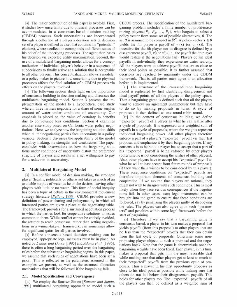
Figure 1. Rausser-Simon multilateral bargaining model, an example.

W02427 PANDE AND MCKEE: VALUING MODELING CERTAINTY

3 of 13

W02427

round. If the solution to the proposer’s (Pi) constrainedmaximization problem yields Pi at least the expected utilityfrom proceeding to the next round, he proposes this solutionto his maximization problem. Otherwise, he proposes avector that is rejected by one or more players.

2.3. An Example

[17] Consider a three-player bargaining problem over atwo-dimensional policy variable [Adams et al., 1996;Thoyer et al., 2001]. The two-dimensional policy variableplane identifies the space of possible agreement policyvectors. Each player has a most preferred location, calledhis ideal point. The game is assumed to be long but finite,with a total of T possible rounds of bargaining. At eachround t < T, nature chooses at random a player Pi withprobability wi (this identifies a player’s access probabilityand is interpreted as the player’s bargaining power), suchthat

PIwi = 1. Player Pi, chosen at random, makes a

proposal xPi 2 @@. If the proposal is acceptable to all, theproposal forms the solution vector. Otherwise, the bargain-ing moves to the next round. The game continues untilperiod T, where if the proposal propounded is not acceptedall the players get their disagreement payoffs. I j,t identifiesthe reservation payoff in round t of each player Pj. This canalso be seen as a player’s expected payoff from playing thesubgame from the t + 1 period onward. Pj’s reservationpayoff in some round T � t is also his disagreement payoff,when the players fail to agree upon a solution if thenegotiations go to round T.[18] For Pi’s proposal to be accepted in any arbitrary

round t, it has to yield other players a payoff level greaterthan their expected payoff (obtained by playing the sub-game t + 1 from then onward). At t = T in Figure 1, P2

proposes x2,T with probability w2, yielding P1 his disagree-ment payoff (xi,Tis the solution to Pi’s constrained maximi-zation problem in round T). Similarly, P1 would get hisdisagreement payoff when P3 proposes x

3,Twith probabilityw3. P1 realizes a strictly higher payoff when he proposesx1,T with positive probability w1. Thus the payoff that P1

expects in the final round when he is in the penultimateround, and hence his reservation payoff in round T � 1, isgreater than his reservation payoff in the final round (or hisdisagreement payoff). By backward induction, P1’s reser-vation utility in round t will then be greater than that inround t + 1. Similarly, this can be shown to be the same forall the other players. Accordingly, the distance between theplayers’ proposals will be closer in round t than in roundt + 1. Thus if T is large enough, the distance between theproposals of players in round 1 will be arbitrarily small, andin the limit as T ! 1, the solution to the game isdeterministic and x* is implemented with probability one.

2.4. Specific Remarks

[19] From the above example it may appear that only thefirst round has any meaning. This is true if players imple-ment the game in the same way, but it assumes they aresufficiently smart to calculate all the possible moves of allthe other players up to some finitely large number of roundsinto the future. The calculation of other players’ moves isequivalent to knowing their equilibrium strategies in anyround, where a strategy of a player is defined as how hewould react to a proposal. The players therefore propose a

solution in first round itself, since they would know (by theirown convergence argument) that the solution is the onlyproposal agreeable to all. However the assumption of suffi-cient far sightedness and capacity to know others’ strategiesis too strict. Thus by inverse labeling proposal rounds in themodel specification (with the round when a solution isachieved labeled as the last round of proposals and theround when players face their disagreement payoffs as thefirst round), we have assumed that the game is implementedfrom a round of disagreement and the players proposeonward to a solution. This implicitly assumes that they canonly calculate other players’ strategies one round at a time.[20] Note that both the kinds of round labeling have the

same set of equilibrium strategies in each round, irrespectiveof its label. Hence the arguments of convergence to a solutionare the same in a mathematical sense and the solution of thegame is the same. Thus labeling does not matter if thesolution point is of interest, though it is important in defininghow the game is implemented. Therefore, by relabeling theproposal rounds as in the subsection of model specificationand convergence, we can also follow from the above examplewhy the game converges to a solution.[21] The following two case studies show how uncertainty

influences the equilibrium solution. The first case study is asimple three-farmer problem under uncertainty. It showshow uncertainty due to conveyance loss enters the param-eters of a player’s profit function. This modification in thepreference structure is not due to a change in the player’spreference, but to his belief of uncertainty in conveyanceloss. It therefore shows, in simple and explicit terms, thatthe final allocation solution is affected by a change inpreference parameters of a player (in addition to second-order effects on other players) due to the presence ofuncertainty. This similarly happens in the second case study.Here we consider the effect of uncertainty (at differentlevels) in the degree of water right transferability on thebargaining solution of California water policy negotiationsas studied by Adams et al. [1996]. However unlike the firstcase study, the effect of change in preference parameters(due to uncertainty) of one player on the bargaining solutionis not dominant because second-order effects on otherplayers are stronger. Thus these two case studies serve ascomplimentary examples for clear exposition of the effectsof uncertainty on consensus-based decision making and thevalue that can be derived by reducing such uncertainty.

3. Case Study I: Three-Farmer Problem

[22] In this case study, we consider bargaining betweenthree farmers, {F1, F2, F3}, over sharing some surplusamount of water, X. Their production functions are assumedto be quadratic in water input [Chakravorty and Roumasset,1991; Burness and Quirk, 1979]. There is a surplus ofwater, X, from which the farmers bargain to obtain a share,and which is available at a constant price k. The farmers selltheir products at an exogenously fixed and given price p.The profit function for player i is therefore given by,

pi xið Þ ¼ p a1i x2i þ b1i xi þ c1i

� �� kxi

¼ aix2i þ bixi þ ci; and

X3i¼1

xi ¼ X ð1Þ

4 of 13

W02427 PANDE AND MCKEE: VALUING MODELING CERTAINTY W02427

Since the profit functions are concave in water input, ai 0.[23] One of the three farmers also faces a conveyance loss

from the source of the surplus to his point of use. Such aloss in conveyance is stochastic in nature. In a bargainingsituation, the farmer facing such a loss then bargains for anamount such that, after the loss of a physical quantity ofwater in conveyance to his cropland, he receives the profithe expected at the bargaining table. Let g represent thepercentage of water arriving at the farm so that the absoluteloss in conveyance is given by (1 � g)xi. Thus, duringdiscussions at the bargaining table the profit (or payoff)function of the loss-facing farmer, Fi, would take the form(along the lines of Chakravorty and Roumasset [1991]):

pi xi; gð Þ ¼ aig2x2i þ pb1i g � k� �

xi þ ci

[24] The loss-facing farmer attempts to maximize hisexpected profit over various values of g, where the truevalue of g is unknown. Therefore the farmer’s expectedprofit function depends solely on his perception of thechances with which various losses can occur. This canfurther be translated, for simplicity, to a continuous proba-bility density function yi(g,a) as a ‘‘model’’ to predictlosses. Here a denotes some abstract parameter set todescribe the density function. We further assume that theexpectation of loss using yi(g,a) is unbiased, or the trueexpectation of loss coincides with the predicted expectation.Thus a farmer’s expected profit function yields the form:

pia xið Þ ¼ E pi xið Þ;a½ � ¼Z

pi xi; gð Þyi g;að Þ@g

¼ aix2i

Zg2yi g;að Þ@g þ pb1i

Zgyi g;að Þ@g � k

� �xi þ ci

¼ ai m2 að Þ þ �g2 að Þ� �

x2i þ pb1i �g að Þ � k� �

xi þ ci ð2Þ

Here

m2 að Þ ¼Z

g � x½ �2yi g;að Þ@g � 0

�g að Þ ¼Z

gyi g;að Þ@g

where g(a) is the expected loss over the density defined bythe parameter a. If the true expected loss is denoted by x,then by assumption g(a) = x. m2 (a) is the variance of thedensity function defined by a. The variance describes thespread of the distribution about the expectation, which inturn explains the uncertainty in the modeled loss being closeto the expectation. The larger the variance, the greater will

be the uncertainty that the predicted loss is close to theexpected. Note that g = 0 (a is a null set) for the case whennone of the farmers is facing a conveyance loss.

3.1. Payoffs

[25] Ideal payoffs are defined as the payoffs that the farmersreceive if there is no scarcity condition. Thus the ideal payoffof any farmer Fi is his maximized profit, the solution to theunconstrained profit maximization problem:

pideali ¼ max

xipi xið Þ : 0 xi;

or

pideali;a ¼ max

xipia xið Þ : 0 xi;

for the case with uncertainty in xi. Their ideal pointallocation, xi

ideal, in the set of possible alternatives is definedas the solution to the first-order necessary condition of theabove maximization problem. Disagreement payoffs arecalculated using an unbiased lottery system to allocate theavailable surplus.

3.2. Simulations

[26] To investigate and demonstrate the effect of uncer-tainty in conveyance loss on the bargaining solution for thiscase study, we choose the coefficient values (in equations (1)and (2)) as {ai

1, bi1, ci, p, k, X} = {�1,3,1,1,1,1}. It is

assumed that each of the three farmers has perfect knowl-edge about the payoff functions of the other two and thatthere is in place an enforcement mechanism under theCBDM framework that requires all the farmers to be honestabout their payoff functions. All the farmers have equalrepresentation in the sense that they all have equal bargain-ing power (w1 = w2 = w3 = 1/3). If the negotiations fail, theywill get their disagreement payoffs. Therefore it is assumedthat if the negotiations fail, the surplus is allocated through alottery system. To simplify matters, we consider the farmersto have the same payoff function coefficients.3.2.1. Bargaining Under No Loss Conditions[27] As one would expect, the farmers share the total

surplus equally and each receives an equal allocation ofwater under ideal conditions, disagreement conditions, andequilibrium conditions.[28] The first row of Table 1 shows the ideal payoffs and

ideal allocations. Payoffs in this row are unconstrainedmaximized profits, and the water allocations are its max-imizers. The second row contains the disagreement payoffsand corresponding certainty equivalent water allocation. Thethird row shows the equilibrium solution. Although thereservation payoffs are not that low (since we have N = 3),risk neutral farmers still negotiate because their equilibriumpayoffs are higher than their disagreement payoffs. More-over, due to the limited quantity of surplus water (because, inorder to achieve ideal payoffs, they would require a total ofthree units of surplus), their equilibrium payoffs are less thantheir ideal payoffs.3.2.2. Bargaining Under Loss Conditions WithNo Uncertainty[29] We now suppose that the first farmer faces an

uncertain loss in conveyance. His expectation of the amount

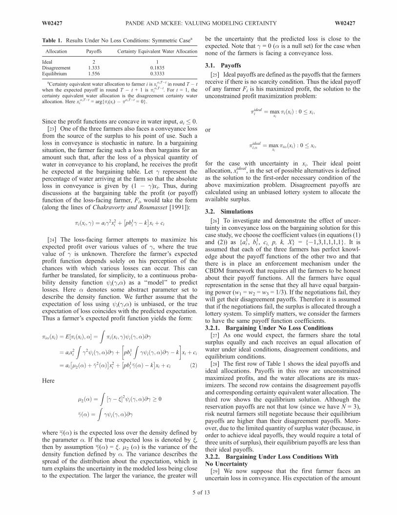
Table 1. Results Under No Loss Conditions: Symmetric Casea

Allocation Payoffs Certainty Equivalent Water Allocation

Ideal 2 1Disagreement 1.333 0.1835Equilibrium 1.556 0.3333

aCertainty equivalent water allocation to farmer i is xio,T�t in round T � t

when the expected payoff in round T � t + 1 is pio,T�t. For t = 1, the

certainty equivalent water allocation is the disagreement certainty waterallocation. Here xi

o,T�t = arg{pi(xi) � po,T�t = 0}.

W02427 PANDE AND MCKEE: VALUING MODELING CERTAINTY

5 of 13

W02427

of water delivered to the cropland is assumed to have avalue of x = 0.9. Characterization of uncertainties inconveyance of water must accommodate the possibility ofeither seepage losses from a conveyance system or ground-water return flows entering the conveyance system. There-fore the variation in losses is assumed to be greater than 1 toallow for both losses or gains in conveyance. Whilecounterintuitive, in practice gains are occasionally observedin canal flows. m2(a) = 0, as we are considering nouncertainty in loss predictions.[30] The ideal payoff for the first farmer is reduced

because of these conveyance losses. The entry of loss inhis payoff function changes his expected payoff such thathis ideal allocation is greater than when he faces no losses.Moreover, his equilibrium payoff also decreases.[31] Another interesting observation for this simulation is

that the equilibrium payoffs of farmers 2 and 3 are lowerthan their equilibrium payoffs when farmer 1 does not face aloss condition (Table 1). The loss affects all farmer profits,even though only one of the farmers faces a loss inconveyance. This observation, however, is subject to thechoice of parameters identifying the profit functions of thefarmers used in the simulations. Table 2 shows that the totalsocial benefit (sum of equilibrium payoffs of all the farmers),which is 4.587 units, is less than the total social benefit underthe no-loss condition (4.668 units, from Table 1). Thisreduction is due to both the reduced equilibrium payoff offarmer 1 and to a reduction in equilibrium payoffs of theother two farmers. It is from this reduction of equilibriumpayoffs that we find the economic utility of reducingmodeling uncertainty, as the next section explains.3.2.3. Bargaining Under Loss ConditionsWith Uncertainty[32] We now extend the previous section by varying the

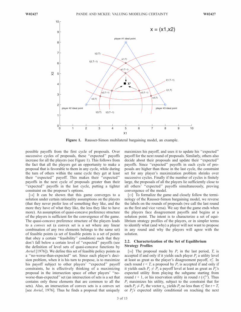
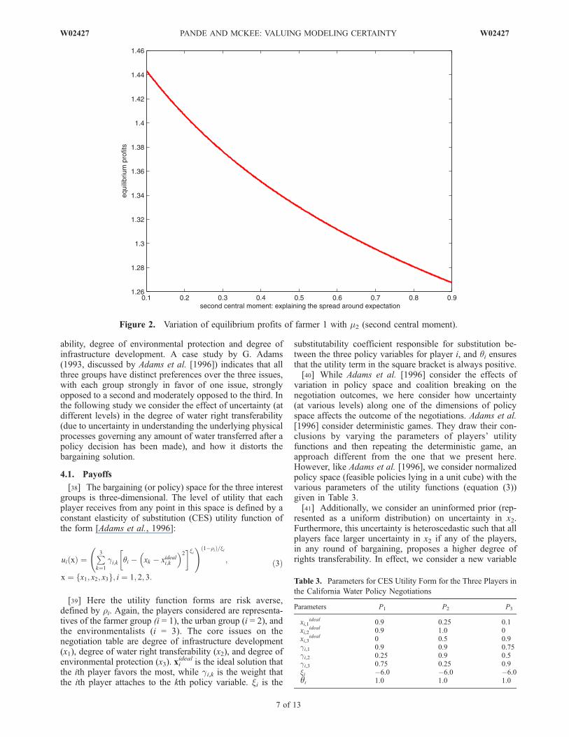
level of uncertainty in the losses that farmer 1 may face, toshow how farmer 1’s equilibrium payoff varies with uncer-tainty. We vary m2 from 0.1 to 0.9. Varying m2 is equivalentto varying a, which defines a particular probability densityof losses. In essence, varying m2 provides various percep-tions of loss uncertainty and therefore a loss ‘‘model’’ withvarying prediction uncertainty. These perceptions mathe-matically represent the estimated density functions of los-ses. Estimation in turn is never a reality but only anapproximation to it. A better approximation explains realitybetter, and hence a better estimated density is closer to the‘‘true’’ density function. Even though the smallest achiev-able uncertainty would be bounded from below by theactual uncertainty (which exists in nature), we have arbi-trarily selected this lower bound to be 0.1. The previousassumption that the expected predicted loss coincides withthe actual expectation is maintained for all predictor densi-

ties (g(a) = x = 0.9). This means that the loss expected (in amathematical sense) under a particular model (defined by a)is the same as the ‘‘true’’ loss expectation.[33] Not surprisingly, the larger the variance in farmer 1’s

prediction of his loss, the lower is his equilibrium profit.Both the equilibrium total profit and the marginal profitdecline as the variance of predicted losses in conveyanceincreases. This can be partially attributed to farmer 1’s idealpayoff. The greater the uncertainty, the smaller is his idealpayoff. This in turn reduces his disagreement payoff, whichcauses his equilibrium payoff to fall. Figure 2 illustrates thisbehavior of equilibrium payoff of farmer 1.[34] If we assume that a unit increment in the equilibrium

payoff for all the farmers increases their indirect utility bythe same amount, the increment in farmer 1’s equilibriumpayoff with some decrement in uncertainty is the maximumthat he is willing to pay for that decrement in uncertainty.Thus Figure 2, in a way, plots the willingness to pay offfarmer 1 for certainty when in negotiation for a share in theavailable surplus of water.

3.3. Specific Remarks

[35] Some readers may ponder, Why not have the farmersauction off the surplus water and split the revenues amongstthemselves? This may fetch a better price and thus a largerrevenue surplus to be shared rather than bargain over thedivision of surplus at some a priori fixed price. Note that wehave not assumed in the paper that the players have a prioripartial ownership of the surplus. Thus farmers have tounanimously agree to auction off the surplus first, beforesplitting the revenues. However, then this collective deci-sion will depend heavily upon a later process of revenuedistribution. The players therefore still have to go through aprocess that ‘‘fairly’’ distributes the revenue, such as aconsensus-based decision-making process.[36] What if the owner of the surplus decides to auction

the surplus to a farmer with the highest bid rather thanallowing the farmers to bargain for a share at some fairprice? Though economically efficient, this option will be instark contrast to the intent of this paper (which is to providea modeling framework for consensus-based decision mak-ing). Auctions are the purest form of markets. While abargaining approach leads to a Pareto inferior (option A isPareto inferior to option B when option A, in comparison tooption B, makes at least one party worse off even if all theother parties are better off) solution to auctions, the lattertotally ignores the equity dimension of revenue distribution[Thomas and Wilson, 2002]. This lack of equity dimensionin auctions is evident in its monopolistic nature [Bulow andKlemperer, 1996]. Multilateral bargaining at least allows fora platform where possible arrangements for equitable dis-tribution can be discussed [Krishna and Serrano, 1996].

4. Case Study II: California Water PolicyNegotiations

[37] Here we study a more realistic scenario of Californiawater policy negotiations as considered by Adams et al.[1996]. In the early 1990s, representatives from agriculturalwater agencies, urban water agencies, and environmentalgroups attempted to forge a consensus-based solution overissues relating to California water policy. The major issuesin the negotiations included degree of water right transfer-

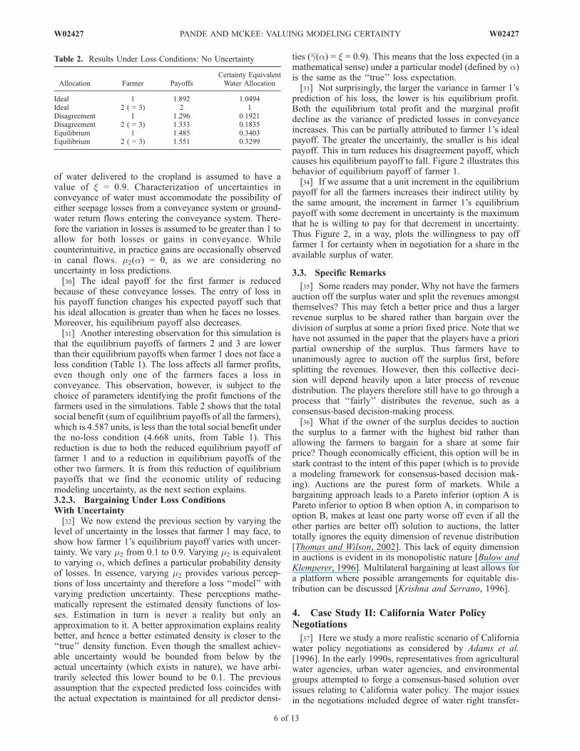
Table 2. Results Under Loss Conditions: No Uncertainty

Allocation Farmer PayoffsCertainty EquivalentWater Allocation

Ideal 1 1.892 1.0494Ideal 2 ( = 3) 2 1Disagreement 1 1.296 0.1921Disagreement 2 ( = 3) 1.333 0.1835Equilibrium 1 1.485 0.3403Equilibrium 2 ( = 3) 1.551 0.3299

6 of 13

W02427 PANDE AND MCKEE: VALUING MODELING CERTAINTY W02427

ability, degree of environmental protection and degree ofinfrastructure development. A case study by G. Adams(1993, discussed by Adams et al. [1996]) indicates that allthree groups have distinct preferences over the three issues,with each group strongly in favor of one issue, stronglyopposed to a second and moderately opposed to the third. Inthe following study we consider the effect of uncertainty (atdifferent levels) in the degree of water right transferability(due to uncertainty in understanding the underlying physicalprocesses governing any amount of water transferred after apolicy decision has been made), and how it distorts thebargaining solution.

4.1. Payoffs

[38] The bargaining (or policy) space for the three interestgroups is three-dimensional. The level of utility that eachplayer receives from any point in this space is defined by aconstant elasticity of substitution (CES) utility function ofthe form [Adams et al., 1996]:

ui xð Þ ¼P3k¼1

gi;k qi � xk � xideali;k

� 2� �xi ! 1�rið Þ=xi

;

x ¼ x1; x2; x3f g; i ¼ 1; 2; 3:

ð3Þ

[39] Here the utility function forms are risk averse,defined by ri. Again, the players considered are representa-tives of the farmer group (i = 1), the urban group (i = 2), andthe environmentalists (i = 3). The core issues on thenegotiation table are degree of infrastructure development(x1), degree of water right transferability (x2), and degree ofenvironmental protection (x3). xi

ideal is the ideal solution thatthe ith player favors the most, while gi,k is the weight thatthe ith player attaches to the kth policy variable. xi is the

substitutability coefficient responsible for substitution be-tween the three policy variables for player i, and qi ensuresthat the utility term in the square bracket is always positive.[40] While Adams et al. [1996] consider the effects of

variation in policy space and coalition breaking on thenegotiation outcomes, we here consider how uncertainty(at various levels) along one of the dimensions of policyspace affects the outcome of the negotiations. Adams et al.[1996] consider deterministic games. They draw their con-clusions by varying the parameters of players’ utilityfunctions and then repeating the deterministic game, anapproach different from the one that we present here.However, like Adams et al. [1996], we consider normalizedpolicy space (feasible policies lying in a unit cube) with thevarious parameters of the utility functions (equation (3))given in Table 3.[41] Additionally, we consider an uninformed prior (rep-

resented as a uniform distribution) on uncertainty in x2.Furthermore, this uncertainty is heteroscedastic such that allplayers face larger uncertainty in x2 if any of the players,in any round of bargaining, proposes a higher degree ofrights transferability. In effect, we consider a new variable

Figure 2. Variation of equilibrium profits of farmer 1 with m2 (second central moment).

Table 3. Parameters for CES Utility Form for the Three Players in

the California Water Policy Negotiations

Parameters P1 P2 P3

xi,1ideal 0.9 0.25 0.1

xi,2ideal 0.9 1.0 0

xi,3ideal 0 0.5 0.9

gi,1 0.9 0.9 0.75gi,2 0.25 0.9 0.5gi,3 0.75 0.25 0.9xi �6.0 �6.0 �6.0qi 1.0 1.0 1.0

W02427 PANDE AND MCKEE: VALUING MODELING CERTAINTY

7 of 13

W02427

x02 = x2r, where the random variable r � U[1 � p/2,1 + p/2],which all three players see as effective degree of water righttransferability. Assuming all the players are expected utilitymaximizers, their transformed utility functions are of theform:

u0i x; pð Þ ¼ Er�U 1�p=2;1þp=2½ �

Xk¼1;3

gi;k qi � xk � xideali;k

� 2� �xi

þ gi;2 qi � rx2 � xideali;2

� 2� �xi! 1�rið Þ=xi!;

rx2 2 0; 1½ �8x2ð4Þ

Here p identifies a level of uncertainty in exact knowledgeof the attainable degree of water rights transferability, x2.For p = 0, we have our base case, i.e., a case with nouncertainty. In order to obtain disagreement utility levels forall the players, we assume that under the bargainingbreakdown condition, all three players receive their leastfeasible utility levels ui

o(xio,p), where

uoi xoi ; p�

¼ minx2 0;1½ �3

u0i x; pð Þ

[42] Since the ideal policy solution for each player isconsidered as a parameter (given in Table 3), it is straight-forward to note that ui

ideal(xiideal, p) is the ideal utility level

for each of the players.

4.2. Simulations

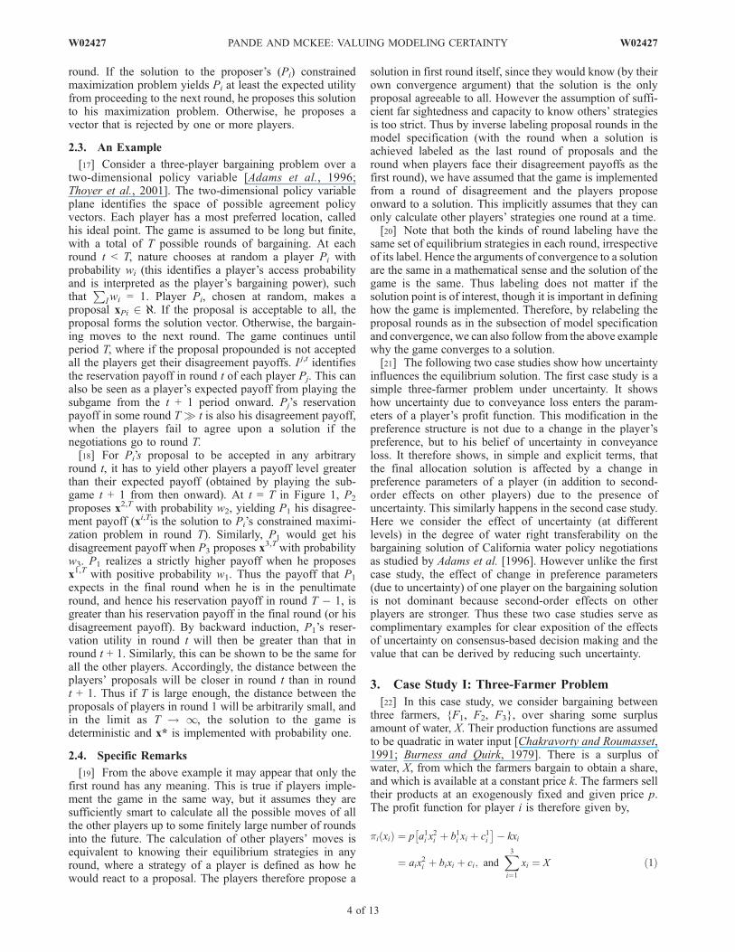
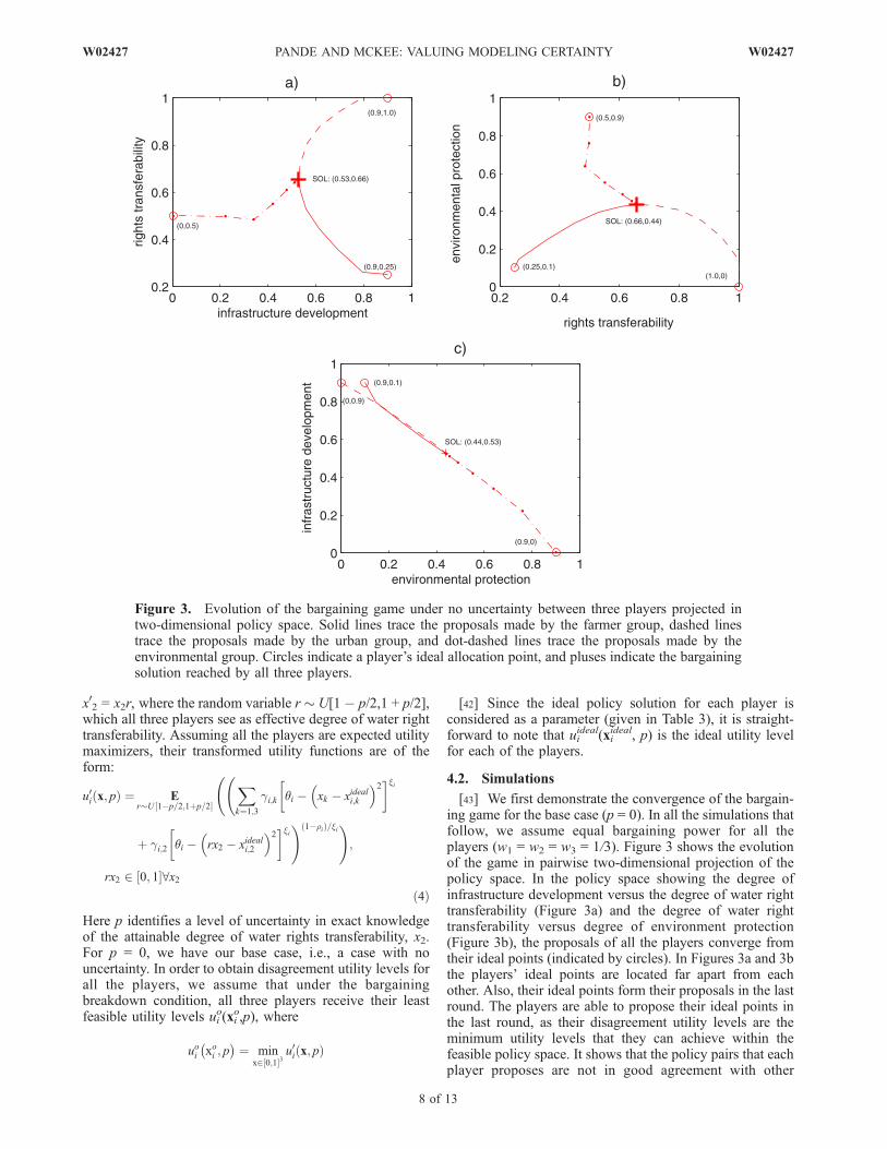
[43] We first demonstrate the convergence of the bargain-ing game for the base case (p = 0). In all the simulations thatfollow, we assume equal bargaining power for all theplayers (w1 = w2 = w3 = 1/3). Figure 3 shows the evolutionof the game in pairwise two-dimensional projection of thepolicy space. In the policy space showing the degree ofinfrastructure development versus the degree of water righttransferability (Figure 3a) and the degree of water righttransferability versus degree of environment protection(Figure 3b), the proposals of all the players converge fromtheir ideal points (indicated by circles). In Figures 3a and 3bthe players’ ideal points are located far apart from eachother. Also, their ideal points form their proposals in the lastround. The players are able to propose their ideal points inthe last round, as their disagreement utility levels are theminimum utility levels that they can achieve within thefeasible policy space. It shows that the policy pairs that eachplayer proposes are not in good agreement with other

Figure 3. Evolution of the bargaining game under no uncertainty between three players projected intwo-dimensional policy space. Solid lines trace the proposals made by the farmer group, dashed linestrace the proposals made by the urban group, and dot-dashed lines trace the proposals made by theenvironmental group. Circles indicate a player’s ideal allocation point, and pluses indicate the bargainingsolution reached by all three players.

8 of 13

W02427 PANDE AND MCKEE: VALUING MODELING CERTAINTY W02427

players’ proposals. However, in the policy pair space ofdegree of environmental protection versus degree of infra-structure development (Figure 3c), the policy pairs proposedby the farmer and urban groups almost coincide. However,those are in disagreement with proposals made by theenvironmental group.[44] Such behavior is due to the preference structure of all

the players over the issues. Farmer and urban groups areidentical in their preference for degree of infrastructure devel-opment, moderately differ over degree of environment protec-tion, and strongly differ over water right transferability. On theother hand, the environmental group’s preference over all ofthe three issues disagrees with both the farmer group and theurban group. This is the reasonwhy the proposals of the farmerand urban group closely agree with each other in Figure 3c anddisagree in Figures 3a and 3b, while proposals of the environ-mental group never agree with the other two groups.[45] We now simulate the bargaining game under varying

uncertainty levels, p > 0. Uncertainty levels considered rangefrom p = 0.02 to p = 0.5, with increments of 0.02. Theexpected utility level for each player is numerically calcu-lated by uniformly sampling r from the interval [1� p/ 2,1 +p/2] 10,000 times and then evaluating the mean of u00i (x, p) asan estimate, u0i (x, p), of ui

0(x, p) (equation (4)). Here

u00i x; p; rj�

¼ X

k¼1;3

gi;k qi � xk � xideali;k

� 2� �xi

þ gi;2 qi � rjx2 � xideali;2

� 2� �xi! 1�rið Þ=xi!

u0i x; pð Þ ¼ 1

10000

X10000j¼1

u00i x; p; rj�

rj � U 1� p=2; 1þ p=2½ �; rjx2 2 0; 1½ �

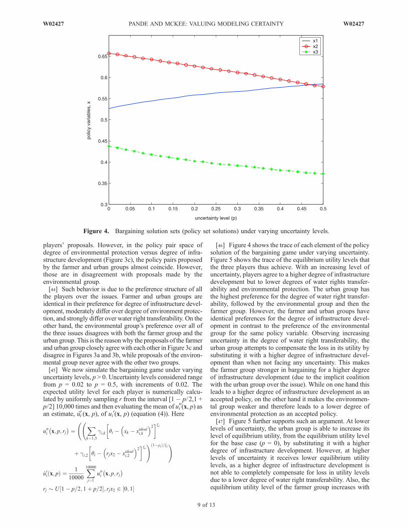
[46] Figure 4 shows the trace of each element of the policysolution of the bargaining game under varying uncertainty.Figure 5 shows the trace of the equilibrium utility levels thatthe three players thus achieve. With an increasing level ofuncertainty, players agree to a higher degree of infrastructuredevelopment but to lower degrees of water rights transfer-ability and environmental protection. The urban group hasthe highest preference for the degree of water right transfer-ability, followed by the environmental group and then thefarmer group. However, the farmer and urban groups haveidentical preferences for the degree of infrastructure devel-opment in contrast to the preference of the environmentalgroup for the same policy variable. Observing increasinguncertainty in the degree of water right transferability, theurban group attempts to compensate the loss in its utility bysubstituting it with a higher degree of infrastructure devel-opment than when not facing any uncertainty. This makesthe farmer group stronger in bargaining for a higher degreeof infrastructure development (due to the implicit coalitionwith the urban group over the issue). While on one hand thisleads to a higher degree of infrastructure development as anaccepted policy, on the other hand it makes the environmen-tal group weaker and therefore leads to a lower degree ofenvironmental protection as an accepted policy.[47] Figure 5 further supports such an argument. At lower

levels of uncertainty, the urban group is able to increase itslevel of equilibrium utility, from the equilibrium utility levelfor the base case (p = 0), by substituting it with a higherdegree of infrastructure development. However, at higherlevels of uncertainty it receives lower equilibrium utilitylevels, as a higher degree of infrastructure development isnot able to completely compensate for loss in utility levelsdue to a lower degree of water right transferability. Also, theequilibrium utility level of the farmer group increases with

Figure 4. Bargaining solution sets (policy set solutions) under varying uncertainty levels.

W02427 PANDE AND MCKEE: VALUING MODELING CERTAINTY

9 of 13

W02427

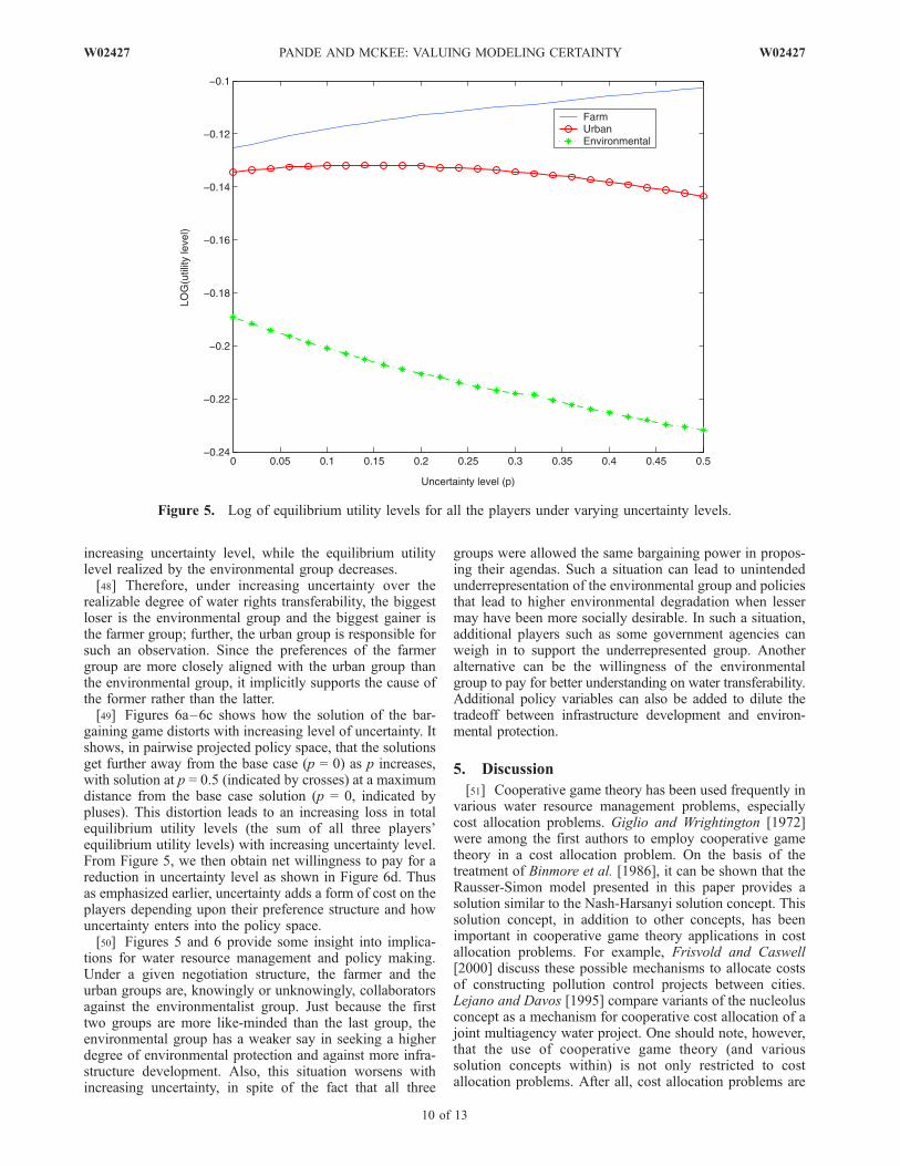
increasing uncertainty level, while the equilibrium utilitylevel realized by the environmental group decreases.[48] Therefore, under increasing uncertainty over the

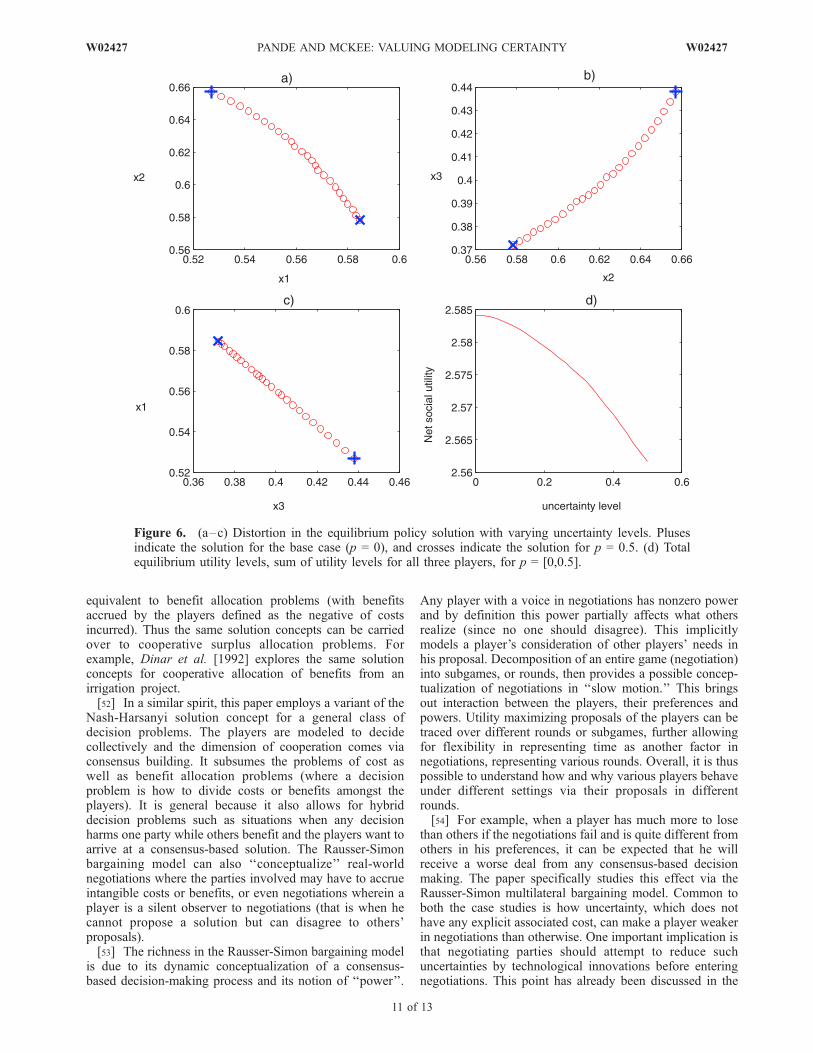
realizable degree of water rights transferability, the biggestloser is the environmental group and the biggest gainer isthe farmer group; further, the urban group is responsible forsuch an observation. Since the preferences of the farmergroup are more closely aligned with the urban group thanthe environmental group, it implicitly supports the cause ofthe former rather than the latter.[49] Figures 6a–6c shows how the solution of the bar-

gaining game distorts with increasing level of uncertainty. Itshows, in pairwise projected policy space, that the solutionsget further away from the base case (p = 0) as p increases,with solution at p = 0.5 (indicated by crosses) at a maximumdistance from the base case solution (p = 0, indicated bypluses). This distortion leads to an increasing loss in totalequilibrium utility levels (the sum of all three players’equilibrium utility levels) with increasing uncertainty level.From Figure 5, we then obtain net willingness to pay for areduction in uncertainty level as shown in Figure 6d. Thusas emphasized earlier, uncertainty adds a form of cost on theplayers depending upon their preference structure and howuncertainty enters into the policy space.[50] Figures 5 and 6 provide some insight into implica-

tions for water resource management and policy making.Under a given negotiation structure, the farmer and theurban groups are, knowingly or unknowingly, collaboratorsagainst the environmentalist group. Just because the firsttwo groups are more like-minded than the last group, theenvironmental group has a weaker say in seeking a higherdegree of environmental protection and against more infra-structure development. Also, this situation worsens withincreasing uncertainty, in spite of the fact that all three

groups were allowed the same bargaining power in propos-ing their agendas. Such a situation can lead to unintendedunderrepresentation of the environmental group and policiesthat lead to higher environmental degradation when lessermay have been more socially desirable. In such a situation,additional players such as some government agencies canweigh in to support the underrepresented group. Anotheralternative can be the willingness of the environmentalgroup to pay for better understanding on water transferability.Additional policy variables can also be added to dilute thetradeoff between infrastructure development and environ-mental protection.

5. Discussion

[51] Cooperative game theory has been used frequently invarious water resource management problems, especiallycost allocation problems. Giglio and Wrightington [1972]were among the first authors to employ cooperative gametheory in a cost allocation problem. On the basis of thetreatment of Binmore et al. [1986], it can be shown that theRausser-Simon model presented in this paper provides asolution similar to the Nash-Harsanyi solution concept. Thissolution concept, in addition to other concepts, has beenimportant in cooperative game theory applications in costallocation problems. For example, Frisvold and Caswell[2000] discuss these possible mechanisms to allocate costsof constructing pollution control projects between cities.Lejano and Davos [1995] compare variants of the nucleolusconcept as a mechanism for cooperative cost allocation of ajoint multiagency water project. One should note, however,that the use of cooperative game theory (and varioussolution concepts within) is not only restricted to costallocation problems. After all, cost allocation problems are

Figure 5. Log of equilibrium utility levels for all the players under varying uncertainty levels.

10 of 13

W02427 PANDE AND MCKEE: VALUING MODELING CERTAINTY W02427

equivalent to benefit allocation problems (with benefitsaccrued by the players defined as the negative of costsincurred). Thus the same solution concepts can be carriedover to cooperative surplus allocation problems. Forexample, Dinar et al. [1992] explores the same solutionconcepts for cooperative allocation of benefits from anirrigation project.[52] In a similar spirit, this paper employs a variant of the

Nash-Harsanyi solution concept for a general class ofdecision problems. The players are modeled to decidecollectively and the dimension of cooperation comes viaconsensus building. It subsumes the problems of cost aswell as benefit allocation problems (where a decisionproblem is how to divide costs or benefits amongst theplayers). It is general because it also allows for hybriddecision problems such as situations when any decisionharms one party while others benefit and the players want toarrive at a consensus-based solution. The Rausser-Simonbargaining model can also ‘‘conceptualize’’ real-worldnegotiations where the parties involved may have to accrueintangible costs or benefits, or even negotiations wherein aplayer is a silent observer to negotiations (that is when hecannot propose a solution but can disagree to others’proposals).[53] The richness in the Rausser-Simon bargaining model

is due to its dynamic conceptualization of a consensus-based decision-making process and its notion of ‘‘power’’.

Any player with a voice in negotiations has nonzero powerand by definition this power partially affects what othersrealize (since no one should disagree). This implicitlymodels a player’s consideration of other players’ needs inhis proposal. Decomposition of an entire game (negotiation)into subgames, or rounds, then provides a possible concep-tualization of negotiations in ‘‘slow motion.’’ This bringsout interaction between the players, their preferences andpowers. Utility maximizing proposals of the players can betraced over different rounds or subgames, further allowingfor flexibility in representing time as another factor innegotiations, representing various rounds. Overall, it is thuspossible to understand how and why various players behaveunder different settings via their proposals in differentrounds.[54] For example, when a player has much more to lose

than others if the negotiations fail and is quite different fromothers in his preferences, it can be expected that he willreceive a worse deal from any consensus-based decisionmaking. The paper specifically studies this effect via theRausser-Simon multilateral bargaining model. Common toboth the case studies is how uncertainty, which does nothave any explicit associated cost, can make a player weakerin negotiations than otherwise. One important implication isthat negotiating parties should attempt to reduce suchuncertainties by technological innovations before enteringnegotiations. This point has already been discussed in the

Figure 6. (a–c) Distortion in the equilibrium policy solution with varying uncertainty levels. Plusesindicate the solution for the base case (p = 0), and crosses indicate the solution for p = 0.5. (d) Totalequilibrium utility levels, sum of utility levels for all three players, for p = [0,0.5].

W02427 PANDE AND MCKEE: VALUING MODELING CERTAINTY

11 of 13

W02427

case studies. Another point is the degree to which it affectsthe players and who else (among the players) may benefitfrom their investments in uncertainty reduction. This iswhere the study of game dynamics becomes important.Both the case studies show that there are some second-order effects on the payoffs of other parties that are notexperiencing uncertainties. This is attributable to implicitcoalition formations due to correlated preference structures.Some parties have a preference structure similar to theaffected party or some parties have correlated preferencesbut different from the affected party. While the former set ofparties loses, the latter set collectively gains due to implicitcooperation against the former. Therefore a cost-sharingmechanism for uncertainty reduction in negotiations forwater resource policy making can be devised on the basisof this model dynamics. Then we can infer uncertainty costs(or implicit benefits) afflicted upon the players and justifycooperation (at least partially for the correlated set ofaffected parties) for cost sharing. For example, unaffectedfarmers may want to partially finance canal lining forreducing conveyance loss for the first farmer, when theyrealize it leads to a win-win situation for all. They can evenapproximate how much they should invest to be net gainers.[55] Uncertainty, especially in decision making in water

resource management, can easily occur due to naturalcauses. In both our case studies, it can enter due to losses,insufficient measurement information or approximate modelestimation that disallows exact quantification of waterresource. These case studies additionally show that it canreduce the overall (total) benefits that can be accrued. Thusif no party, especially the affected one, is fully capable offinancing uncertainty reduction measures, some governmentagency may want to weigh in for overall benefit. Then thismodel can help those government agencies to ascertain theappropriate level of involvement. It also provides someinsight into other roles that such agencies can play. Forexample, in the second case study the environmental groupis the party most affected by uncertainty in water rightstransferability, when it is not the party that is directly facinguncertainty. Further the farmers’ group gains with increas-ing uncertainty levels. It is obvious that the gaining partywill not have any interest in reducing uncertainty and thismay lead to undesirable consequences for the environmentunder increasing uncertainty (in spite of the presence of anenvironmental group in negotiations). A government agen-cy may then want to enter the game dynamics to avoid suchconsequences. It can do so (1) by entering the game as aplayer, (2) by supporting uncertainty reduction measures, or(3) indirectly by making other players aware of the negativeconsequences on the environment and attempt to changetheir attitudes toward the environmental dimension ofpolicy making. Specific interests within a consensus-baseddecision-making process can also be promoted by betterrepresentation of interests at the bargaining table. Uncer-tainty can also be incorporated as an additional policy issuein decision making. A player or an interest group cannot beheld responsible for uncertainty when it is due to naturalcauses. Thus, if uncertainty (faced by some due to naturalcauses) is incorporated as another dimension of decisionmaking, its isolated effects on specific parties can bepartially removed via the game dynamics. However, such

an arrangement is highly unlikely as those players who arenot directly affected by uncertainty (and they know it) willbe reluctant to include it as one of the topics of bargaining.[56] It has to be stressed that the dynamics of the Rausser-

Simon model is of use in modeling consensus-based deci-sion making (with or without uncertainty) when the playersare rational and honest, can be represented as utility max-imizers, and follow the rules (which are set a priori) ofbargaining. The notion of rationality and honesty cannotalways be ensured, since they are hard to quantify. Relatedto the same point is the interpretation of model results. It islimited by the level of accuracy with which its parameters,such as default power, bargaining power, ideal points,perception of uncertainty by various players, each player’slevel of information about other players’ preference, etc. canbe quantified. Bargaining solutions via a multilateral bar-gaining model are sensitive to these parameters in varyingdegree. These sensitivities further depend on the allocationproblems in hand. Thus solutions can be highly uncertaindue to uncertainty in the estimation of model parameters.Also, improvements in the model need to be made byincluding temporal dynamics over successive rounds inplayers’ behavior [Thoyer et al., 2001]. This additionalstructure may help accommodate the pace at which real-world negotiations take place. Finally, bargaining itselfcannot always be recommended as the most appropriateinstitution to facilitate consensus-based decision making. Inreal-world situations, bargaining may not start if all theplayers do not agree upon the terms and conditions ofbargaining (‘‘the parameters’’). Even if bargaining starts, itcan take significant time before any solution is reached, or itmay not even converge. To allay such disadvantages ofbargaining, hybrid institutions can be formulated [Milgrom,1989; Elyakime et al., 1997]. For example, the players maycollectively decide to auction off the surplus in the three-farmer case study, provided they have already negotiated onhow to share future revenues from the sell-off. The playersthen have an additional incentive to reach an agreement onthe shares if they do not want to miss high market prices dueto scarcity.

6. Conclusions

[57] Rausser and Simon’s multilateral bargaining modelwas utilized to simulate the CBDM processes. Two casestudies were analyzed under this framework. Though thesuccess of such a framework crucially depends on theinstitutional structure of the negotiations, it was assumedthat a sufficient legal and institutional framework was inplace to address this requirement. In both case studies, weobserved that the bargaining solution under uncertaintydeviates from the solution under no uncertainty. Moreover,the deviation increases with higher levels of uncertainty.This increasing deviation with uncertainty also quantifiedthe willingness to pay for a reduction in uncertainty.

[58] Acknowledgments. The authors would like to acknowledge theProvo, Utah, office of the US Bureau of Reclamation, the Utah Center forWater Resources Research, and the Utah Water Research Laboratory atUtah State University for their support of this work. We would especiallylike to acknowledge the intellectual contribution of Dr. Roger Hansen of theProvo, Utah, office of the US Bureau of Reclamation. We are also gratefulto the journal’s three anonymous referees for their useful comments.

12 of 13

W02427 PANDE AND MCKEE: VALUING MODELING CERTAINTY W02427

ReferencesAdams, G., G. Rausser, and L. Simon (1996), Modelling multilateralnegotiations: An application to California water policy, J. Econ. BehaviorOrgan., 30, 97–111.

Avriel, M. (1976), Non-linear Programming: Analysis and Methods,Prentice-Hall, Upper Saddle River, N. J.

Becker, N., and K. W. Easter (1995), Water diversions in the Great Lakesbasin analysed in a game theory framework, Water Resour. Manage., 9,221–242.

Becker, N., and K. W. Easter (1997), Water diversion from the Great Lakes:Is a cooperative approach possible?, Water Resour. Dev., 13, 53–65.

Binmore, K., A. Rubinstein, and A. Wolinsky (1986), The Nash bargainingsolution in economic modeling, Rand J. Econ., 17, 176–188.

Bulow, J., and P. Klemperer (1996), Auctions versus negotiations, Am.Econ. Rev., 86, 180–194.

Burness, H. S., and J. P. Quirk (1979), Appropriative water rights and theefficient allocation of resources, Am. Econ. Rev., 69, 25–37.

Chakravorty, U., and J. Roumasset (1991), Efficient spatial allocation ofirrigation water, Am. J. Agric. Econ., 73, 25–37.

Dinar, A., and R. E. Howitt (1997), Mechanisms for allocation of environ-mental control cost: Empirical tests of acceptability and stability,J. Environ. Manage., 49, 183–203.

Dinar, A., and A. Xepapadaes (2002), Regulating water quality andquantity in irrigated agriculture: Learning by investing under asymmetricinformation, Environ. Model. Assess., 7, 17–27.

Dinar, A., A. Ratner, and D. Yaron (1992), Evaluating cooperative gametheory in water resources, Theory Decis., 32, 1–20.

Elyakime, B., J. Laffont, L. Patrice, and Q. Vuong (1997), Auctions andbargaining: An economic study of timber auctions with secret reservationprices, J. Bus. Econ. Stat., 15, 209–220.

Frisvold, G. B., and M. F. Caswell (2000), Transboundary water manage-ment game-theoretic lessons for projects on the US-Mexico border,Agric. Econ., 24, 101–111.

Giannias, D. A., and J. N. Lekakis (1997), Policy analysis of an amicable,efficient and sustainable inter-country fresh water resource allocation,Ecol. Econ., 21, 231–242.

Giglio, R., and R. Wrightington (1972), Methods for apportioning costsamong participants in regional systems, Water Resour. Res., 8, 1133–1144.

Harsanyi, J. C. (1963), A simplified bargaining model for the n-personcooperative game, Int. Econ. Rev., 4, 194–220.

Hurwicz, L. (1973), The design of mechanisms for resource allocation, Am.Econ. Rev., 63, 1–30.

Israel, M., J. R. Lund, and G. T. Orlob (1994), Cooperative game theory inwater resources, in Water Policy and Management: Solving theProblems, edited by D. G. Fontane and H. N. Tuvel, pp. 569–572,Am. Soc. of Civ. Eng., Reston, Va.

Krishna, V., and R. Serrano (1996), Multilateral bargaining, Rev. Econ.Stud., 63, 61–80.

Lejano, R. P., and C. A. Davos (1995), Cost allocation of multiagency waterresource projects: Game theoretic approaches and case study, WaterResour. Res., 31, 1387–1393.

Lejano, R. P., and C. A. Davos (1999), Cooperative solutions for sustain-able resource management, Environ. Manage., 24, 167–175.

Loehman, E., and A. Dinar (1994), Cooperative solution of local externalityproblems: A case of mechanism design applied to irrigation, J. Environ.Econ. Manage., 26, 235–256.

Lyon, K. S. (1999), The costate variable in natural resource optimal controlproblems, Nat. Resour. Model., 12, 413–426.

Milgrom, P. (1989), Auctions and bidding: A primer, J. Econ. Perspect., 3,3–22.

Nash, J. (1953), Two-person cooperative games, Econometrica, 21, 128–140.

Parros, P. (1999), International water conflicts and depletion of waterresources, in Science Into Policy: Water in the Public Realm, pp. 213–218, edited by E. Kendy, Am. Water Resour. Assoc., Bozeman, Mont.

Pellow, D. (1999), Negotiation and confrontation: Environmental policy-making through consensus, Soc. Nat. Resour., 12, 189–203.

Rausser, G., and L. Simon (1991), A non-cooperative model of collectivedecisionmaking: A multilateral bargaining approach, Working Pap. 618,50 pp., Dep. of Agric. and Resour. Econ., Univ. of Calif., Berkeley.

Rogers, P. (1993), The value of cooperation in resolving international riverbasin disputes, Nat. Resour. Forum, 17, 117–131.

Rubinstein, A. (1982), Perfect equilibrium in a bargaining model, Econo-metrica, 50, 97–109.

Schmeidler, D. (1969), The nucleolus of a characteristic function game,SIAM J. Appl. Math., 17, 1163–1170.

Supalla, R. (2000), A game theoretic analysis of institutional arrangementsfor Platte river management, Water Resour. Dev., 16, 253–264.

Tarboton, D. (1995), Hydrologic scenarios for severe sustained drought insouthwestern United States, Water Resour. Bull., 31, 803–813.

Thomas, C., and B. Wilson (2002), A comparison of auctions and multi-lateral negotiations, Rand J. Econ., 33, 140–155.

Thoyer, S., S. Morardet, P. Rio, L. Simon, R. Goodhue, and G. Rausser(2001), A bargaining model to simulate negotiations between waterusers, J. Artif. Soc. Social Simul., 4 (2), http://www.soc.surrey.ac.uk/JASSS/4/2/6.html.

Utton, A. E. (1996), Regional cooperation: The example of internationalwater systems in the twentieth century, Nat. Resour. J., 36, 151–154.

Whittington, D., and E. McClelland (1992), Opportunities for regional andinternational cooperation in the Nile basin, Water Int., 12, 144–154.

����������������������������M. McKee, Utah Water Research Laboratory, Utah State University,

1600 Canyon Road, Logan, UT 84322-8200, USA. (mmckee@cc.usu.edu)S. Pande, Center for World Food Studies, Faculty of Economics and

Business Administration, Vrije Universiteit, De Boelelaan 1105, NL-1081HV Amsterdam, Netherlands. (s.pande@sow.vu.nl)

W02427 PANDE AND MCKEE: VALUING MODELING CERTAINTY

13 of 13

W02427