at SciVerse ScienceDirect

Journal of Power Sources 236 (2013) 126e137

Contents lists available

Journal of Power Sources

journal homepage: www.elsevier .com/locate/ jpowsour

Validation of a two-phase multidimensional polymer electrolyte membranefuel cell computational model using current distribution measurements

Brian Carnes a,*, Dusan Spernjak b, Gang Luo c, Liang Hao c, Ken S. Chen a, Chao-Yang Wang c,Rangachary Mukundan b, Rodney L. Borup b

a Sandia National Laboratories, PO Box 5800, Albuquerque, NM 87185-0382, USAb Los Alamos National Laboratory, MPA-11, PO Box 1663, Los Alamos, NM 87545, USAc ECEC, The Pennsylvania State University, University Park, PA 16802, USA

h i g h l i g h t s

< Model validation using current distribution data is demonstrated using a 3D, multiphase computational fuel cell model.< Uncertainty in the experimental data is included in the validation in order to improve the model credibility.< Cell voltage agreement (model and experiment) is within 15 mV.< Current distribution error is less than 30% at 80 C operation, with errors up to 60% at low temperature (60 C).

a r t i c l e i n f o

Article history:Received 19 October 2012Received in revised form3 February 2013Accepted 8 February 2013Available online 27 February 2013

Keywords:ValidationPolymer electrolyte membrane fuel cellComputational modelCurrent distribution measurementsUncertainty quantification

* Corresponding author. Tel.: þ1 505 284 1332; faxE-mail address: bcarnes@sandia.gov (B. Carnes).

0378-7753/$ e see front matter � 2013 Elsevier B.V.http://dx.doi.org/10.1016/j.jpowsour.2013.02.039

a b s t r a c t

Validation of computational models for polymer electrolyte membrane fuel cell (PEMFC) performance iscrucial for understanding the limits of the model predictions. We compare predictions from a multiphasePEMFC computational model with experimental data collected under various current density, temper-ature and humidification conditions from a single 50 cm2 PEMFC with a 10 � 10 segmented currentcollector. Both cell voltage and current distribution measurements are used to quantify the predictivecapability of the computational model. Several quantitative measures are used to quantify the error inthe model predictions for current distribution, including root mean square error, maximum/minimumlocal error, and local error averaged from inlet to outlet. The cell voltage predictions were within 15 mVof the experimental data in the current range from 0.1 to 1.2 A cm�2, and the current distributions wereacceptable (less than 30% local error) except for the low temperature case, where the model over-predicted the current distribution. Particular attention was paid to incorporating experimental variabilityinto the model validation process.

� 2013 Elsevier B.V. All rights reserved.

1. Introduction

In the past two decades a large number of computationalmodels have been presented for modeling polymer electrolytemembrane fuel cells (PEMFC). For reviews of the main models andmodeling approaches, see Refs. [1e4] and the references within.While computational models enable unprecedented ability to lookinto the in situ operation of PEMFCs, the limitations of thesemodeling tools must be understood in order to have confidence inthe credibility of the model predictions.

: þ1 505 284 2418.

All rights reserved.

The process of quantifying the degree of credibility of acomputational model is known as model validation [5]. Generallyvalidation consists of comparing the output of the model to datafrom experiments. Here the model has been specifically set up toreproduce the conditions of the experiments; in the case ofPEMFCs, this means that the operating conditions, material prop-erties, dimensions, and experimental outputs must be carefullyspecified in order to provide the best possible inputs to the model.This includes uncertainties, either from random sources (inherentvariability) or from lack of knowledge. Comparison of model andexperiment with properly quantified uncertainty provides a solidbasis to make quantitative determinations.

A wide variety of local (distributed) experimental data has beenobtained, which could potentially be used in model validation,including current density [6e11], species (reactants and products)

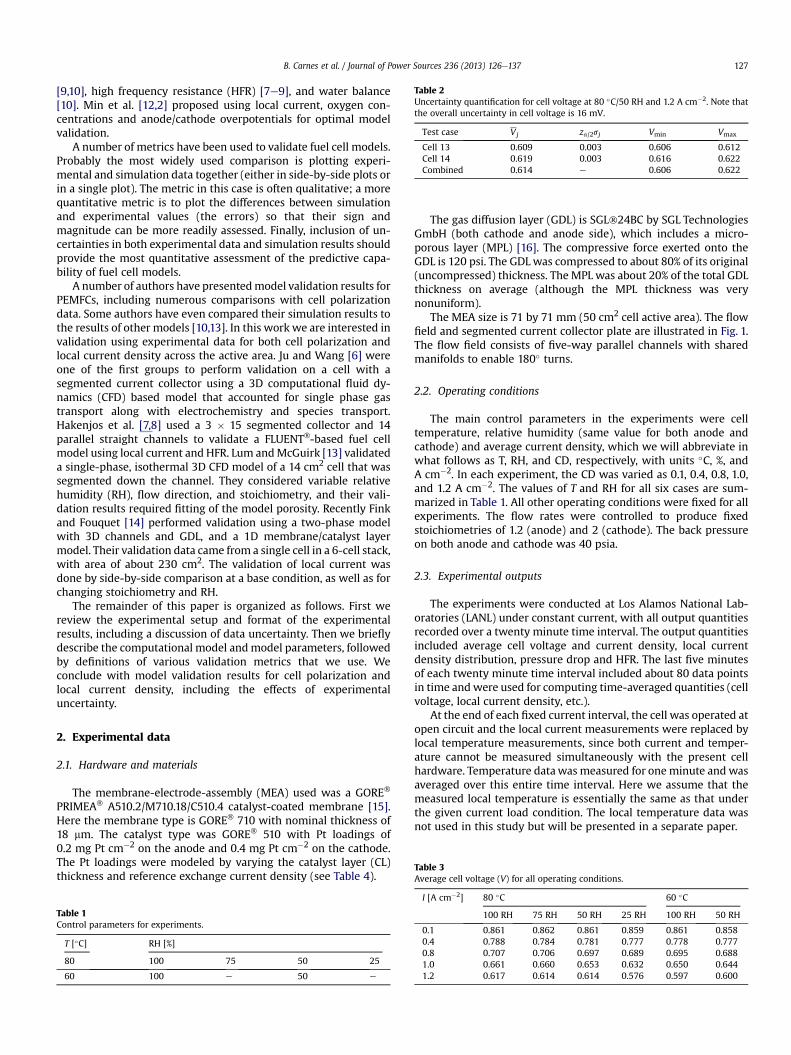
Table 2Uncertainty quantification for cell voltage at 80 �C/50 RH and 1.2 A cm�2. Note thatthe overall uncertainty in cell voltage is 16 mV.

Test case Vj za/2sj Vmin Vmax

Cell 13 0.609 0.003 0.606 0.612Cell 14 0.619 0.003 0.616 0.622Combined 0.614 e 0.606 0.622

B. Carnes et al. / Journal of Power Sources 236 (2013) 126e137 127

[9,10], high frequency resistance (HFR) [7e9], and water balance[10]. Min et al. [12,2] proposed using local current, oxygen con-centrations and anode/cathode overpotentials for optimal modelvalidation.

A number of metrics have been used to validate fuel cell models.Probably the most widely used comparison is plotting experi-mental and simulation data together (either in side-by-side plots orin a single plot). The metric in this case is often qualitative; a morequantitative metric is to plot the differences between simulationand experimental values (the errors) so that their sign andmagnitude can be more readily assessed. Finally, inclusion of un-certainties in both experimental data and simulation results shouldprovide the most quantitative assessment of the predictive capa-bility of fuel cell models.

A number of authors have presentedmodel validation results forPEMFCs, including numerous comparisons with cell polarizationdata. Some authors have even compared their simulation results tothe results of other models [10,13]. In this work we are interested invalidation using experimental data for both cell polarization andlocal current density across the active area. Ju and Wang [6] wereone of the first groups to perform validation on a cell with asegmented current collector using a 3D computational fluid dy-namics (CFD) based model that accounted for single phase gastransport along with electrochemistry and species transport.Hakenjos et al. [7,8] used a 3 � 15 segmented collector and 14parallel straight channels to validate a FLUENT�-based fuel cellmodel using local current and HFR. Lum andMcGuirk [13] validateda single-phase, isothermal 3D CFD model of a 14 cm2 cell that wassegmented down the channel. They considered variable relativehumidity (RH), flow direction, and stoichiometry, and their vali-dation results required fitting of the model porosity. Recently Finkand Fouquet [14] performed validation using a two-phase modelwith 3D channels and GDL, and a 1D membrane/catalyst layermodel. Their validation data came from a single cell in a 6-cell stack,with area of about 230 cm2. The validation of local current wasdone by side-by-side comparison at a base condition, as well as forchanging stoichiometry and RH.

The remainder of this paper is organized as follows. First wereview the experimental setup and format of the experimentalresults, including a discussion of data uncertainty. Then we brieflydescribe the computational model andmodel parameters, followedby definitions of various validation metrics that we use. Weconclude with model validation results for cell polarization andlocal current density, including the effects of experimentaluncertainty.

Table 3Average cell voltage (V) for all operating conditions.

2. Experimental data

2.1. Hardware and materials

The membrane-electrode-assembly (MEA) used was a GORE�

PRIMEA� A510.2/M710.18/C510.4 catalyst-coated membrane [15].Here the membrane type is GORE� 710 with nominal thickness of18 mm. The catalyst type was GORE� 510 with Pt loadings of0.2 mg Pt cm�2 on the anode and 0.4 mg Pt cm�2 on the cathode.The Pt loadings were modeled by varying the catalyst layer (CL)thickness and reference exchange current density (see Table 4).

Table 1Control parameters for experiments.

T [�C] RH [%]

80 100 75 50 25

60 100 e 50 e

The gas diffusion layer (GDL) is SGL�24BC by SGL TechnologiesGmbH (both cathode and anode side), which includes a micro-porous layer (MPL) [16]. The compressive force exerted onto theGDL is 120 psi. The GDL was compressed to about 80% of its original(uncompressed) thickness. The MPL was about 20% of the total GDLthickness on average (although the MPL thickness was verynonuniform).

The MEA size is 71 by 71 mm (50 cm2 cell active area). The flowfield and segmented current collector plate are illustrated in Fig. 1.The flow field consists of five-way parallel channels with sharedmanifolds to enable 180� turns.

2.2. Operating conditions

The main control parameters in the experiments were celltemperature, relative humidity (same value for both anode andcathode) and average current density, which we will abbreviate inwhat follows as T, RH, and CD, respectively, with units �C, %, andA cm�2. In each experiment, the CD was varied as 0.1, 0.4, 0.8, 1.0,and 1.2 A cm�2. The values of T and RH for all six cases are sum-marized in Table 1. All other operating conditions were fixed for allexperiments. The flow rates were controlled to produce fixedstoichiometries of 1.2 (anode) and 2 (cathode). The back pressureon both anode and cathode was 40 psia.

2.3. Experimental outputs

The experiments were conducted at Los Alamos National Lab-oratories (LANL) under constant current, with all output quantitiesrecorded over a twenty minute time interval. The output quantitiesincluded average cell voltage and current density, local currentdensity distribution, pressure drop and HFR. The last five minutesof each twenty minute time interval included about 80 data pointsin time andwere used for computing time-averaged quantities (cellvoltage, local current density, etc.).

At the end of each fixed current interval, the cell was operated atopen circuit and the local current measurements were replaced bylocal temperature measurements, since both current and temper-ature cannot be measured simultaneously with the present cellhardware. Temperature datawas measured for oneminute and wasaveraged over this entire time interval. Here we assume that themeasured local temperature is essentially the same as that underthe given current load condition. The local temperature data wasnot used in this study but will be presented in a separate paper.

I [A cm�2] 80 �C 60 �C

100 RH 75 RH 50 RH 25 RH 100 RH 50 RH

0.1 0.861 0.862 0.861 0.859 0.861 0.8580.4 0.788 0.784 0.781 0.777 0.778 0.7770.8 0.707 0.706 0.697 0.689 0.695 0.6881.0 0.661 0.660 0.653 0.632 0.650 0.6441.2 0.617 0.614 0.614 0.576 0.597 0.600

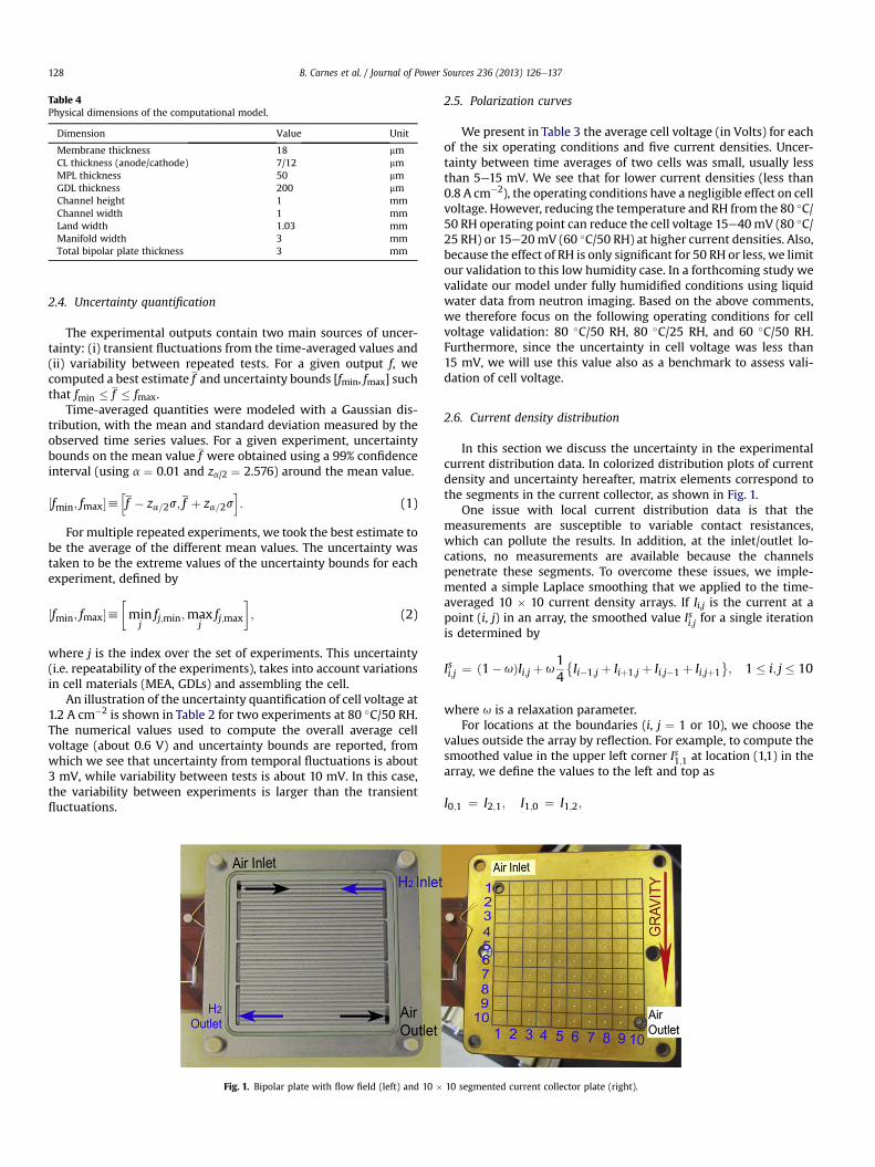
Table 4Physical dimensions of the computational model.

Dimension Value Unit

Membrane thickness 18 mmCL thickness (anode/cathode) 7/12 mmMPL thickness 50 mmGDL thickness 200 mmChannel height 1 mmChannel width 1 mmLand width 1.03 mmManifold width 3 mmTotal bipolar plate thickness 3 mm

B. Carnes et al. / Journal of Power Sources 236 (2013) 126e137128

2.4. Uncertainty quantification

The experimental outputs contain two main sources of uncer-tainty: (i) transient fluctuations from the time-averaged values and(ii) variability between repeated tests. For a given output f, wecomputed a best estimate f and uncertainty bounds [fmin, fmax] suchthat fmin � f � fmax.

Time-averaged quantities were modeled with a Gaussian dis-tribution, with the mean and standard deviation measured by theobserved time series values. For a given experiment, uncertaintybounds on the mean value f were obtained using a 99% confidenceinterval (using a ¼ 0.01 and za/2 ¼ 2.576) around the mean value.

½fmin; fmax�hhf � za=2s; f þ za=2s

i: (1)

For multiple repeated experiments, we took the best estimate tobe the average of the different mean values. The uncertainty wastaken to be the extreme values of the uncertainty bounds for eachexperiment, defined by

½fmin; fmax�h�min

jfj;min;max

jfj;max

�; (2)

where j is the index over the set of experiments. This uncertainty(i.e. repeatability of the experiments), takes into account variationsin cell materials (MEA, GDLs) and assembling the cell.

An illustration of the uncertainty quantification of cell voltage at1.2 A cm�2 is shown in Table 2 for two experiments at 80 �C/50 RH.The numerical values used to compute the overall average cellvoltage (about 0.6 V) and uncertainty bounds are reported, fromwhich we see that uncertainty from temporal fluctuations is about3 mV, while variability between tests is about 10 mV. In this case,the variability between experiments is larger than the transientfluctuations.

Fig. 1. Bipolar plate with flow field (left) and 10 �

2.5. Polarization curves

We present in Table 3 the average cell voltage (in Volts) for eachof the six operating conditions and five current densities. Uncer-tainty between time averages of two cells was small, usually lessthan 5e15 mV. We see that for lower current densities (less than0.8 A cm�2), the operating conditions have a negligible effect on cellvoltage. However, reducing the temperature and RH from the 80 �C/50 RH operating point can reduce the cell voltage 15e40mV (80 �C/25 RH) or 15e20mV (60 �C/50 RH) at higher current densities. Also,because the effect of RH is only significant for 50 RH or less, we limitour validation to this low humidity case. In a forthcoming study wevalidate our model under fully humidified conditions using liquidwater data from neutron imaging. Based on the above comments,we therefore focus on the following operating conditions for cellvoltage validation: 80 �C/50 RH, 80 �C/25 RH, and 60 �C/50 RH.Furthermore, since the uncertainty in cell voltage was less than15 mV, we will use this value also as a benchmark to assess vali-dation of cell voltage.

2.6. Current density distribution

In this section we discuss the uncertainty in the experimentalcurrent distribution data. In colorized distribution plots of currentdensity and uncertainty hereafter, matrix elements correspond tothe segments in the current collector, as shown in Fig. 1.

One issue with local current distribution data is that themeasurements are susceptible to variable contact resistances,which can pollute the results. In addition, at the inlet/outlet lo-cations, no measurements are available because the channelspenetrate these segments. To overcome these issues, we imple-mented a simple Laplace smoothing that we applied to the time-averaged 10 � 10 current density arrays. If Ii,j is the current at apoint (i, j) in an array, the smoothed value Isi;j for a single iterationis determined by

Isi;j ¼ ð1�uÞIi;j þu14�Ii�1;j þ Iiþ1;j þ Ii;j�1 þ Ii;jþ1

�; 1 � i; j � 10

where u is a relaxation parameter.For locations at the boundaries (i, j ¼ 1 or 10), we choose the

values outside the array by reflection. For example, to compute thesmoothed value in the upper left corner Is1;1 at location (1,1) in thearray, we define the values to the left and top as

I0;1 ¼ I2;1; I1;0 ¼ I1;2;

10 segmented current collector plate (right).

B. Carnes et al. / Journal of Power Sources 236 (2013) 126e137 129

respectively. This insures that the smoothing of boundary valuesonly uses the adjacent values within the array.

In Fig. 2 we illustrate the procedure applied to a matrix at80 �C/50 RH/1.0 CD using three smoothing iterations and u ¼ 0.9.

We see that the smoothing has removed oscillations present inthe raw experimental data arrays from segments with high contactresistance or inlet/outlets (where no current density is measured)and that the characteristics (minimum, maximum, etc.) are mucheasier to discern using the smoothed array. The same smoothingparameters were used in all subsequent plots of measured currentdistribution.

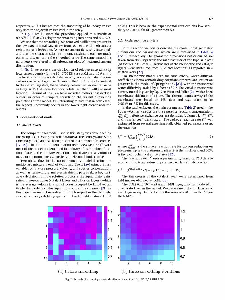
In Fig. 3, we present the distribution of relative uncertainty inlocal current density for the 80 �C/50 RH case at 0.1 and 1.0 A cm�2.The local uncertainty is calculated exactly as we calculated the un-certainty in cell voltage for each point in the 10� 10 array. In contrastto the cell voltage data, the variability between experiments can beas large as 15% at some locations, while less than 5e10% at mostlocations. Because of this, we have included metrics that excludeoutliers in order to compute bounds on the current distributionpredictions of the model. It is interesting to note that in both cases,the highest uncertainty occurs in the lower right corner near theoutlets.

3. Computational model

3.1. Model details

The computational model used in this study was developed bythe group of C.-Y. Wang and collaborators at The Pennsylvania StateUniversity (PSU) and has been presented in a number of references[17e19]. The current implementation uses ANSYS/FLUENT� withmost of the model implemented in a library of user defined func-tions (UDFs). The primary equations solved are conservation ofmass, momentum, energy, species and electrical/ionic charge.

Two-phase flow in the porous zones is modeled using themultiphase mixture model of Wang and Cheng [20] using primaryvariables of mixture pressure, velocity, and species concentration,as well as temperature and electrical/ionic potentials. A key vari-able calculated from the solution process is the liquid water satu-ration in porous zones (catalyst layers and diffusion layers), whichis the average volume fraction of pores occupied by liquid water.While the model includes liquid transport in the channels [21], inthis paper we restrict ourselves to mist transport in the channels,sincewe are only validating against the low humidity data (RH¼ 50

Fig. 2. Example of smoothing current distribut

or 25). This is because the experimental data exhibits low sensi-tivity to T or CD for RH greater than 50.

3.2. Model input parameters

In this section we briefly describe the model input geometricdimensions and parameters, which are summarized in Tables 4and 5, respectively. The geometric dimensions not discussed aretaken from drawings from the manufacturer of the bipolar plates(balticFuelCells GmbH). Thicknesses of the membrane and catalystlayers were measured from SEM cross-sections as reported in arelated work [22].

The membrane model used for conductivity, water diffusioncoefficient, electro-osmotic drag, sorption isotherms and saturationpressure is the model of Springer et al. [23], with the membranewater diffusivity scaled by a factor of 0.7. The variable membranedensity model is given by Eq. 17 inWest and Fuller [24] with a fixedmembrane thickness of 18 mm. The thermal conductivity of themembrane was based on PSU data and was taken to be0.95 W m�1 K for this study.

In the catalyst layers, the main parameters (Table 5) used in theButlereVolmer kinetics are the reference reactant concentrationscrefH2 ; c

refO2 , reference exchange current densities (volumetric) jrefa ; jrefc ,

and transfer coefficients aa, ac. The cathode reaction rate jrefc wasestimated from several experimentally obtained parameters usingthe equation

jrefc ¼ jrefc;surf

�mPt

tc

�ECSA; (3)

where jrefc;surf is the surface reaction rate for oxygen reduction onplatinum, mPt is the platinum loading, tc is the thickness, and ECSAis the electrochemical surface area [22].

The reaction rate jrefc uses a parameter Ec based on PSU data torepresent the temperature dependence of the cathode reaction

jrefc ¼ jref ;353:15c exp½ � Ecð1=T � 1=353:15Þ�:The thicknesses of the catalyst layers were determined from

SEM images obtained at LANL [22].The GDL (SGL24BC) contains an MPL layer, which is modeled as

a separate layer in the model. We determined the thicknesses ofeach layer using a total substrate thickness of 250 mmwith a 50 mmthick MPL.

ion data (A cm�2) at 80 �C/50 RH/1.0 CD.

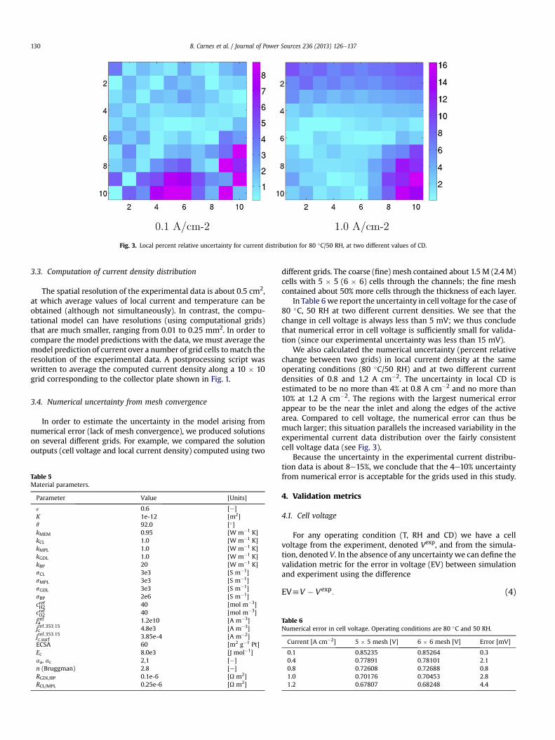
Fig. 3. Local percent relative uncertainty for current distribution for 80 �C/50 RH, at two different values of CD.

B. Carnes et al. / Journal of Power Sources 236 (2013) 126e137130

3.3. Computation of current density distribution

The spatial resolution of the experimental data is about 0.5 cm2,at which average values of local current and temperature can beobtained (although not simultaneously). In contrast, the compu-tational model can have resolutions (using computational grids)that are much smaller, ranging from 0.01 to 0.25 mm2. In order tocompare the model predictions with the data, we must average themodel prediction of current over a number of grid cells tomatch theresolution of the experimental data. A postprocessing script waswritten to average the computed current density along a 10 � 10grid corresponding to the collector plate shown in Fig. 1.

3.4. Numerical uncertainty from mesh convergence

In order to estimate the uncertainty in the model arising fromnumerical error (lack of mesh convergence), we produced solutionson several different grids. For example, we compared the solutionoutputs (cell voltage and local current density) computed using two

Table 5Material parameters.

Parameter Value [Units]

ε 0.6 [e]K 1e-12 [m2]q 92.0 [�]kMEM 0.95 [W m�1 K]kCL 1.0 [W m�1 K]kMPL 1.0 [W m�1 K]kGDL 1.0 [W m�1 K]kBP 20 [W m�1 K]sCL 3e3 [S m�1]sMPL 3e3 [S m�1]sGDL 3e3 [S m�1]sBP 2e6 [S m�1]crefH2 40 [mol m�3]crefO2 40 [mol m�3]jrefa 1.2e10 [A m�3]jref ;353:15c 4.8e3 [A m�3]jref ;353:15c;surf 3.85e-4 [A m�2]ECSA 60 [m2 g�1 Pt]Ec 8.0e3 [J mol�1]aa, ac 2,1 [e]n (Bruggman) 2.8 [e]RGDL/BP 0.1e-6 [U m2]RCL/MPL 0.25e-6 [U m2]

different grids. The coarse (fine) mesh contained about 1.5 M (2.4 M)cells with 5 � 5 (6 � 6) cells through the channels; the fine meshcontained about 50% more cells through the thickness of each layer.

In Table 6 we report the uncertainty in cell voltage for the case of80 �C, 50 RH at two different current densities. We see that thechange in cell voltage is always less than 5 mV; we thus concludethat numerical error in cell voltage is sufficiently small for valida-tion (since our experimental uncertainty was less than 15 mV).

We also calculated the numerical uncertainty (percent relativechange between two grids) in local current density at the sameoperating conditions (80 �C/50 RH) and at two different currentdensities of 0.8 and 1.2 A cm�2. The uncertainty in local CD isestimated to be no more than 4% at 0.8 A cm�2 and no more than10% at 1.2 A cm�2. The regions with the largest numerical errorappear to be the near the inlet and along the edges of the activearea. Compared to cell voltage, the numerical error can thus bemuch larger; this situation parallels the increased variability in theexperimental current data distribution over the fairly consistentcell voltage data (see Fig. 3).

Because the uncertainty in the experimental current distribu-tion data is about 8e15%, we conclude that the 4e10% uncertaintyfrom numerical error is acceptable for the grids used in this study.

4. Validation metrics

4.1. Cell voltage

For any operating condition (T, RH and CD) we have a cellvoltage from the experiment, denoted Vexp, and from the simula-tion, denoted V. In the absence of any uncertainty we can define thevalidation metric for the error in voltage (EV) between simulationand experiment using the difference

EVhV � Vexp: (4)

Table 6Numerical error in cell voltage. Operating conditions are 80 �C and 50 RH.

Current [A cm�2] 5 � 5 mesh [V] 6 � 6 mesh [V] Error [mV]

0.1 0.85235 0.85264 0.30.4 0.77891 0.78101 2.10.8 0.72608 0.72688 0.81.0 0.70176 0.70453 2.81.2 0.67807 0.68248 4.4

Fig. 4. Mid-plane of the cathode GDL at 80 �C, 50% RH and 1.0 A cm�2: water concentration (mol m�3) and liquid saturation (�).

B. Carnes et al. / Journal of Power Sources 236 (2013) 126e137 131

However, as discussed in Section 2.4, variability in the experi-mental data can be modeled using an interval ½Vexp

min;Vexpmax�. In this

case we can define the validation metric UEV as the signed distancebetween V and this interval

UEVh

8><>:

V � Vexpmax V > Vexp

max;

V � Vexpmin V < Vexp

min;

0 else:

(5)

Thus if Vexpmin � V � Vexp

max, then the metric returns zero, since thesimulation value lies within the uncertainty. Positive/negativemetrics imply overshoot/undershoot of the interval of uncertaintyaround the experimental data.

4.2. Current density distribution

The validation metrics for current density distribution are basedon the local errors in the current density defined by

EihIi � Iexpi ; i ¼ 1;.;N (6)

Fig. 5. Mid-plane of the membran

where N¼ 100 is the total number of segments. The metrics are theroot mean square relative error,

RMSh100Iavg

Xi

jEij2N

!1=2

; (7)

and minimum/maximum of the relative error,

MINhP5ðf100Ei=IigiÞ; (8)

MAXhP95ðf100Ei=IigiÞ; (9)

where Pr denotes the r-th percentile of a set of data (0 � r � 100).We have excluded the bottom/top 5% of the errors, in order toexclude extreme values which may be associated with noise ineither the experiment or simulation.

We also define metrics based on averaging the local segmentedcurrent along each horizontal row of segments (as shown in Fig. 1)in order to consider the average current along the overall flow di-rection from inlet to outlet (top to bottom). These are defined

e: CD and water content (l).

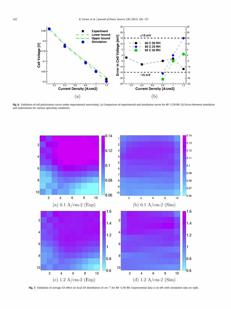
Fig. 6. Validation of cell polarization curves under experimental uncertainty. (a) Comparison of experimental and simulation curves for 80 �C/50 RH. (b) Errors between simulationand experiments for various operating conditions.

Fig. 7. Validation of average CD effect on local CD distribution (A cm�2) for 80 �C/50 RH. Experimental data is on left with simulation data on right.

B. Carnes et al. / Journal of Power Sources 236 (2013) 126e137132

B. Carnes et al. / Journal of Power Sources 236 (2013) 126e137 133

exactly as in Eqs. (7)e(9) except that we replace the N ¼ 100 datapoints by the

ffiffiffiffiN

p¼ 10 row averages of the simulation and

experimental data.Finally we note that inclusion of experimental uncertainty in

local current data can easily be done by extending the simpledefinition of the error using the same formula for cell voltage in (5).

5. Results

5.1. Example simulation output

Before we present the validation results, we begin with somerepresentative results of the simulation output obtained using thecomputational model. We focus on a specific operating point at80 �C, 50 RH and 1.0 CD.

In Fig. 4 we plot the concentration of total water and liquidwater saturation along the mid-plane of the cathode GDL. The totalwater concentration increases from inlet to outlet, mainly from theproduct water. Liquid water accumulates in the lower half of theGDL, predominantly under the land areas and along the edges ofthe cell.

In Fig. 5 we plot the distribution of CD and water content l

(number of water molecules per sulfonic acid site in the mem-brane) in the center plane of the membrane. The region ofmaximum current is in the lower center area, similar to the

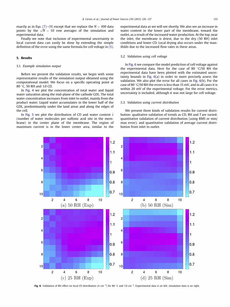
Fig. 8. Validation of RH effect on local CD distribution (A cm�2) for 80 �C a

experimental data as wewill see shortly. We also see an increase inwater content in the lower part of the membrane, toward theoutlet, as a result of the increasedwater production. At the top, nearthe inlet, the membrane is driest, due to the dry (50 RH) inletconditions and lower CD. Local drying also occurs under the man-ifolds due to the increased flow rates in these areas.

5.2. Validation using cell voltage

In Fig. 6 we compare themodel prediction of cell voltage againstthe experimental data. Here for the case of 80 �C/50 RH theexperimental data have been plotted with the estimated uncer-tainty bounds in Fig. 6(a) in order to more precisely assess thevalidation. We also plot the error for all cases in Fig. 6(b). For thecase of 80 �C/50 RH the errors is less than 15mV, and in all cases it iswithin 20 mV of the experimental voltage. For the error metrics,uncertainty is included, although it was not large for cell voltage.

5.3. Validation using current distribution

We present three kinds of validation results for current distri-bution: qualitative validation of trends as CD, RH and T are varied;quantitative validation of current distribution (using RMS or min/max error); and quantitative validation of average current distri-bution from inlet to outlet.

nd 1.0 cm�2. Experimental data is on left; simulation data is on right.

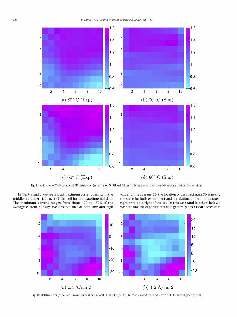
Fig. 9. Validation of T effect on local CD distribution (A cm�2) for 50 RH and 1.2 cm�2. Experimental data is on left with simulation data on right.

B. Carnes et al. / Journal of Power Sources 236 (2013) 126e137134

In Fig. 7(a and c) we see a local maximum current density in themiddle- to upper-right part of the cell for the experimental data.The maximum current ranges from about 120 to 150% of theaverage current density. We observe that at both low and high

Fig. 10. Relative error (experiment minus simulation) in local CD at 80 �C/

values of the average CD, the location of the maximum CD is nearlythe same for both experiment and simulation, either in the upper-right or middle-right of the cell. In this case (and in others below),we note that the experimental data generally has a local decrease in

50 RH. Percentiles used for cutoffs were 5/95 for lower/upper bounds.

Fig. 11. Relative error (experiment minus simulation) in local CD at 1.0 cm�2. Percentiles used for cutoffs were 5/95 for lower/upper bounds.

B. Carnes et al. / Journal of Power Sources 236 (2013) 126e137 135

current in the bottom-right corner, near the location of the cathodeoutlet. This feature is not evident in any of the simulation results.One possible explanation for this discrepancy could be channelflooding, which the model used cannot predict, since we are notactivating the two-phase channel sub-model.

In Fig. 8(a and c) we plot the effect of decreasing RH atCD ¼ 1.0 A cm�2 and 80 �C for the experimental data. Here we seethat the local maximum CD shifts downward with decreasing RHfrom 50 to 25. We observe a similar shift in maximum CD in thesimulation data (b, d), along with similar values of the maximumCD. However, the simulation again does not predict the drop inlocal current near the cathode outlet. The model also underpredictsthe current along the top row of segments, near the inlets, at 25 RH.This may be to excessive drying in the model near the inlet.

In Fig. 9(left panels) we plot the effect of temperature at 50 RHand 1.0 CD for the experimental data. We see that as the temper-ature is decreased from 80 to 60 �C, the maximum CD shifts towardthe top (inlets). We observe a similar shift for the simulation data,although the current distribution is much more uniform at 60 �C,failing to reach the same maximum or minimum CD. The difficultywith the predictions at low temperature could be due to the largeamount of temperature-dependent properties in the model; some

Fig. 12. Error metrics for current distribu

of these properties may be well calibrated at 80 �C, but less so atother temperatures. Another possibility is the choice of boundaryconditions. We assume in this work that a uniform temperatureboundary condition is valid; however, the cell surface in fact hassome variation in temperature.

In Fig. 10 we plot the distribution of percent relative error inthe prediction of segmented (i.e. local) current for the case of80 �C/50 RH at two different current densities. The errors aregenerally within 20% of the experimental values, with largest un-derestimation along the top row of segments (inlet region) andlargest overestimation in the lower left area (near the anode outlet).Such plots of actual errors can be useful in pinpointing regions ofmaximum disagreement between simulations and experiments.

In Fig.11we present the distribution in CD error at a fixed averageCD of 1.0 A cm�2 at two other operating conditions (80 �C/25 RH and60 �C/50RH). At 25RH, the local errors are again generallywithin 20%of the experimental values. However, at 60 �C, overprediction of localcurrent reaches 60% near the outlet and on the left side of the cell.

In Fig. 12(a) we plot global error metrics for RMS relative errorfor a number of operating conditions. These are used to integratethe local information in Figs. 10 and 11 into global data that can bemore easily summarized. For example, at lower CD, the errors are

tion at various operating conditions.

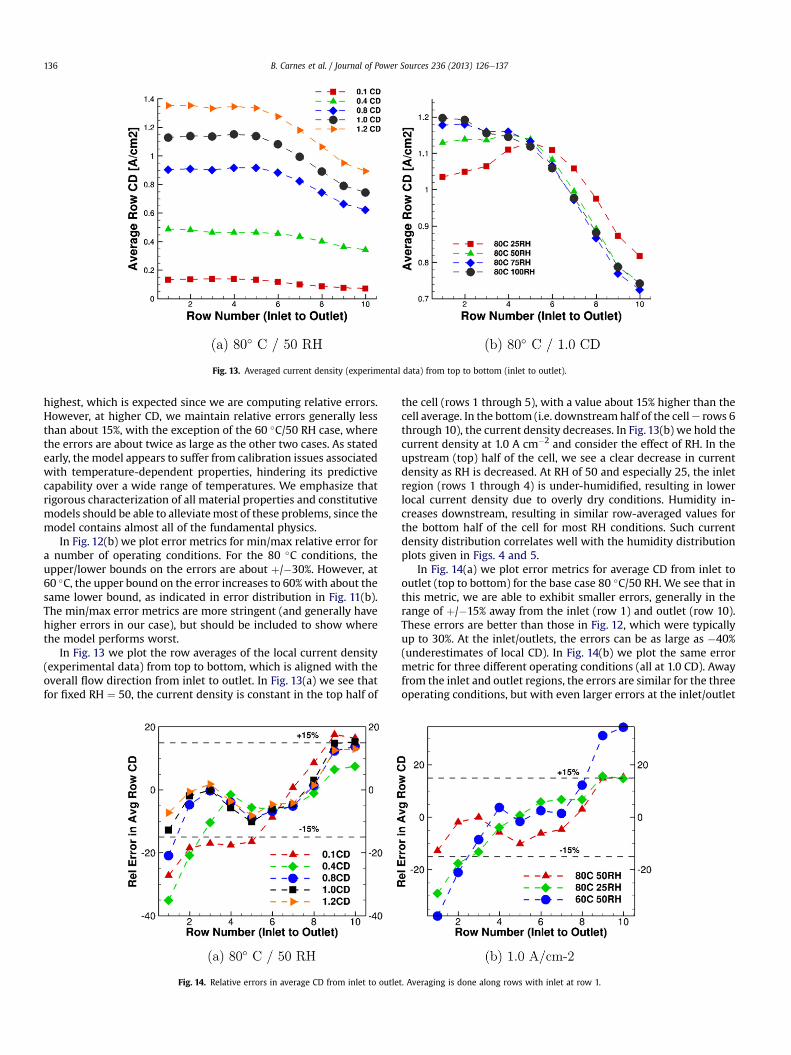
Fig. 13. Averaged current density (experimental data) from top to bottom (inlet to outlet).

B. Carnes et al. / Journal of Power Sources 236 (2013) 126e137136

highest, which is expected since we are computing relative errors.However, at higher CD, we maintain relative errors generally lessthan about 15%, with the exception of the 60 �C/50 RH case, wherethe errors are about twice as large as the other two cases. As statedearly, the model appears to suffer from calibration issues associatedwith temperature-dependent properties, hindering its predictivecapability over a wide range of temperatures. We emphasize thatrigorous characterization of all material properties and constitutivemodels should be able to alleviatemost of these problems, since themodel contains almost all of the fundamental physics.

In Fig. 12(b) we plot error metrics for min/max relative error fora number of operating conditions. For the 80 �C conditions, theupper/lower bounds on the errors are about þ/�30%. However, at60 �C, the upper bound on the error increases to 60%with about thesame lower bound, as indicated in error distribution in Fig. 11(b).The min/max error metrics are more stringent (and generally havehigher errors in our case), but should be included to show wherethe model performs worst.

In Fig. 13 we plot the row averages of the local current density(experimental data) from top to bottom, which is aligned with theoverall flow direction from inlet to outlet. In Fig. 13(a) we see thatfor fixed RH ¼ 50, the current density is constant in the top half of

Fig. 14. Relative errors in average CD from inlet to outle

the cell (rows 1 through 5), with a value about 15% higher than thecell average. In the bottom (i.e. downstream half of the celle rows 6through 10), the current density decreases. In Fig. 13(b) we hold thecurrent density at 1.0 A cm�2 and consider the effect of RH. In theupstream (top) half of the cell, we see a clear decrease in currentdensity as RH is decreased. At RH of 50 and especially 25, the inletregion (rows 1 through 4) is under-humidified, resulting in lowerlocal current density due to overly dry conditions. Humidity in-creases downstream, resulting in similar row-averaged values forthe bottom half of the cell for most RH conditions. Such currentdensity distribution correlates well with the humidity distributionplots given in Figs. 4 and 5.

In Fig. 14(a) we plot error metrics for average CD from inlet tooutlet (top to bottom) for the base case 80 �C/50 RH. We see that inthis metric, we are able to exhibit smaller errors, generally in therange of þ/�15% away from the inlet (row 1) and outlet (row 10).These errors are better than those in Fig. 12, which were typicallyup to 30%. At the inlet/outlets, the errors can be as large as �40%(underestimates of local CD). In Fig. 14(b) we plot the same errormetric for three different operating conditions (all at 1.0 CD). Awayfrom the inlet and outlet regions, the errors are similar for the threeoperating conditions, but with even larger errors at the inlet/outlet

t. Averaging is done along rows with inlet at row 1.

B. Carnes et al. / Journal of Power Sources 236 (2013) 126e137 137

regions. We conclude that the increase in the errors for the 60 �Ccondition shown in Fig. 12(b) is mainly a result of larger errors inthe inlet/outlet regions. As mentioned above, these inlet/outleterrors could be from incorrect temperature boundary conditions,temperature-dependent material properties, or possibly liquidwater formation in the channels.

6. Conclusions

We have presented model validation results based on currentdistribution data and a multiphase PEMFC computational model.The cell voltage validation results were acceptable, generallywith errors less than 15 mV. For current distribution validation,we presented the results using a number of validation metrics,including RMS error, min/max local error, and averaged errors alongthe flow direction from inlet to outlet. The best results obtainedwere at the 80 �C condition (both 25 and 50 RH), where the localerror was less than 30% and RMS error was less than 15%. Largererrors at 60 �C/50 RH (up to 60% overestimation of local current)appear to be localized to the inlet/outlet regions. These errors maybe the result of incorrect temperature boundary conditions,improperly calibrated temperature-dependent material properties,liquid water in the gas channels, or some other unknown cause.

Inclusion of uncertainty in the validation metrics was possiblebecause of repeated experimental data. The uncertainty allowed usto more precisely quantify the validity of the computational model,through the use of intervals of uncertainty around the experimentaldata, which represent the range of variability present in the ex-periments and measurements.

We conclude with several remarks and suggestions for futurework. First, model validation requires a careful interaction betweenmodelers and experimentalists; experimental conditions must befaithfully reproduced in simulations, model input characterizationrequires knowledge of the materials used (especially withtemperature-dependent material properties), and uncertainty inexperimental measurements must be quantified. The latter wasachieved in this work by repeating the characterization tests inseveral cells re-assembled using new materials (MEAs and GDLs).

Second, while cell voltage data is a good starting point forvalidation models, other outputs such as current distribution datashould be used. The higher the resolution in such local data, thegreater the need becomes to account for the inherent uncertainty inthe data and in the computational models.

For future work, we intend to further integrate the validationmetrics into forms that can be presented succinctly, as well asdefine additional well-characterized experiments suitable formodel validation. Further, some parameters in the present modelwill be discussed in more detail, taking into account the predictedwater distribution and using neutron imaging measurements as anadditional validation metric.

Acknowledgments

Sandia is a multiprogram laboratory operated by Sandia Cor-poration, a Lockheed Martin Company, for the United StatesDepartment of Energy’s National Nuclear Security Administrationunder contract DE-AC04-94AL85000.

Nomenclature

crefH2 reference hydrogen concentration

crefO2 reference oxygen concentrationECSA electro-chemical surface areaEc temperature coefficient in jrefcjrefa reference anode exchange current density

jref ;353:15c reference cathode exchange current density

jref ;353:15c;surf reference surface Pt exchange current density

K permeabilityk thermal conductivityN number of segmentsn Bruggeman exponentR contact resistanceRMS root mean square errorV cell voltage

Greek symbolsl membrane water contentε porosityq contact angles electrical conductivityaa, ac transfer coefficients

Subscripts/superscriptsref reference valueexp experimentalsim simulation

References

[1] S. Mazumder, J. Cole, J. Electrochem. Soc. (2003).[2] W.Tao, C.Min, X. Liu, Y.He, B. Yin,W. Jiang, J. Power Sources 160 (2006) 359e373.[3] P. Sui, S. Kumar, N. Djilali, J. Power Sources 180 (2008) 410e422.[4] T. Berning, M. Odgaard, S. Kaer, J. Electrochem. Soc. 156 (2009) B1301eB1311.[5] W. Oberkampf, C. Roy, Verification and Validation in Scientific Computing,

Cambridge University Press, 2010.[6] H. Ju, C.-Y. Wang, J. Electrochem. Soc. 151 (2004) A1954eA1960.[7] A. Hakenjos, K. Tüber, J. Schumacher, C. Hebling, Fuel Cells 3 (2004) 185e189.[8] A. Hakenjos, C. Hebling, J. Power Sources 145 (2005) 307e311.[9] Q. Dong, M.M. Mench, S. Cleghorn, U. Beuscher, J. Electrochem. Soc. (2005).

[10] P. Sui, S. Kumar, N. Djilali, J. Power Sources 180 (2008) 423e432.[11] H. Ly, E. Birgersson, M. Vynnycky, A. Sasmito, J. Electrochem. Soc. (2009).[12] C. Min, Y. He, X. Liu, B. Yin, W. Jiang, W. Tao, J. Power Sources 160 (2006)

374e385.[13] K. Lum, J. McGuirk, J. Power Sources 143 (2005) 103e124.[14] C. Fink, M. Fouquet, Electrochim. Acta 56 (2011).[15] S. Cleghorn, J. Kolde, W. Liu, Handbook of Fuel Cells: Fundamentals, Tech-

nology and Applications, vol. 3, John Wiley & Sons, pp. 566e575.[16] SIGRACET GDL 24 & 25 Series Gas Diffusion Layer, SGL Technologies GmbH,

2007. Technical Report.[17] S. Um, C. Wang, J. Power Sources 124 (2004) 40e51.[18] U. Pasaogullari, C. Wang, K. Chen, J. Electrochem. Soc. 152 (2005) A380eA1582.[19] S. Basu, C.-Y. Wang, K.S. Chen, J. Electrochem. Soc. 156 (2009) B748eB756.[20] C.-Y. Wang, P. Cheng, Int. J. Heat Mass. Transf. 39 (1996) 3607e3618.[21] Y. Wang, S. Basu, C.-Y. Wang, J. Power Sources 179 (2008) 603e617.[22] D. Spernjak, J. Fairweather, R. Mukundan, T. Rockward, R. Borup, J. Power

Sources 214 (2012) 386e398.[23] T. Springer, T. Zawodzinski, S. Gottesfeld, J. Electrochem. Soc. 138 (1991)

2334e2342.[24] A. West, T. Fuller, J. Appl. Electrochem. 26 (1996) 557e565.