�����������������

Citation: Neugebauer, F.;

Antonakakis, M.; Unnwongse, K.;

Parpaley, Y.; Wellmer, J.; Rampp, S.;

Wolters, C.H. Validating EEG, MEG

and Combined MEG and EEG

Beamforming for an Estimation of the

Epileptogenic Zone in Focal Cortical

Dysplasia. Brain Sci. 2022, 12, 114.

https://doi.org/10.3390/

brainsci12010114

Academic Editor: Giovanni

Pellegrino

Received: 2 December 2021

Accepted: 6 January 2022

Published: 14 January 2022

Publisher’s Note: MDPI stays neutral

with regard to jurisdictional claims in

published maps and institutional affil-

iations.

Copyright: © 2022 by the authors.

Licensee MDPI, Basel, Switzerland.

This article is an open access article

distributed under the terms and

conditions of the Creative Commons

Attribution (CC BY) license (https://

creativecommons.org/licenses/by/

4.0/).

brainsciences

Article

Validating EEG, MEG and Combined MEG and EEGBeamforming for an Estimation of the Epileptogenic Zone inFocal Cortical Dysplasia

Frank Neugebauer 1,2,*, Marios Antonakakis 1,3, Kanjana Unnwongse 4, Yaroslav Parpaley 5, Jörg Wellmer 4,Stefan Rampp 6,7 and Carsten H. Wolters 1,8

1 Institute for Biomagnetism and Biosignalanalysis, University of Münster, 48149 Münster, Germany;antonakakismar@gmail.com (M.A.); carsten.wolters@uni-muenster.de (C.H.W.)

2 Computing Sciences, Faculty of Information Technology and Communication Sciences, Tampere University,33014 Tampere, Finland

3 School of Electrical and Computer Engineering, Technical University of Crete, 73100 Chania, Greece4 Ruhr-Epileptology, Department of Neurology, University Hospital Knappschaftskrankenhaus,

Ruhr-University, 44892 Bochum, Germany; Kanjana.Unnwongse@kk-bochum.de (K.U.);Joerg.Wellmer@kk-bochum.de (J.W.)

5 Department of Neurosurgery, University Hospital Knappschaftskrankenhaus, Ruhr-University,44892 Bochum, Germany; yaroslav.parpaley@kk-bochum.de

6 Department of Neurosurgery, University Hospital Erlangen, 91054 Erlangen, Germany;stefan.rampp@gmail.com

7 Department of Neurosurgery, University Hospital Halle (Saale), 06097 Halle, Germany8 Otto Creutzfeldt Center for Cognitive and Behavioral Neuroscience, University of Münster, 48149 Münster,

Germany* Correspondence: f.neugebauer@uni-muenster.de

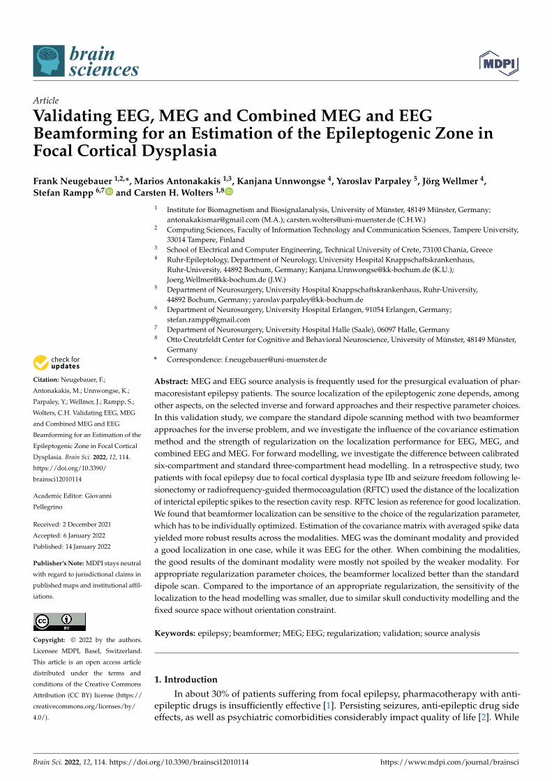
Abstract: MEG and EEG source analysis is frequently used for the presurgical evaluation of phar-macoresistant epilepsy patients. The source localization of the epileptogenic zone depends, amongother aspects, on the selected inverse and forward approaches and their respective parameter choices.In this validation study, we compare the standard dipole scanning method with two beamformerapproaches for the inverse problem, and we investigate the influence of the covariance estimationmethod and the strength of regularization on the localization performance for EEG, MEG, andcombined EEG and MEG. For forward modelling, we investigate the difference between calibratedsix-compartment and standard three-compartment head modelling. In a retrospective study, twopatients with focal epilepsy due to focal cortical dysplasia type IIb and seizure freedom following le-sionectomy or radiofrequency-guided thermocoagulation (RFTC) used the distance of the localizationof interictal epileptic spikes to the resection cavity resp. RFTC lesion as reference for good localization.We found that beamformer localization can be sensitive to the choice of the regularization parameter,which has to be individually optimized. Estimation of the covariance matrix with averaged spike datayielded more robust results across the modalities. MEG was the dominant modality and provideda good localization in one case, while it was EEG for the other. When combining the modalities,the good results of the dominant modality were mostly not spoiled by the weaker modality. Forappropriate regularization parameter choices, the beamformer localized better than the standarddipole scan. Compared to the importance of an appropriate regularization, the sensitivity of thelocalization to the head modelling was smaller, due to similar skull conductivity modelling and thefixed source space without orientation constraint.

Keywords: epilepsy; beamformer; MEG; EEG; regularization; validation; source analysis

1. Introduction

In about 30% of patients suffering from focal epilepsy, pharmacotherapy with anti-epileptic drugs is insufficiently effective [1]. Persisting seizures, anti-epileptic drug sideeffects, as well as psychiatric comorbidities considerably impact quality of life [2]. While

Brain Sci. 2022, 12, 114. https://doi.org/10.3390/brainsci12010114 https://www.mdpi.com/journal/brainsci

Brain Sci. 2022, 12, 114 2 of 22

testing other drugs is often inefficient, surgery has a high seizure-freedom rate afterone year [3,4]. However, among other issues, seizure recurrence within 2–5 years aftersurgery in more than 40% of patients is a major problem [5]. A possible explanation isthat the brain tissue able to generate seizures (often referred to as epileptogenic zone) hasbeen resected, destroyed, or disconnected only incompletely or that it has been (more orless narrowly) missed. As an advanced diagnostic tool, magnetoencephalography (MEG)and/or electroencephalography (EEG) source analysis may contribute to resolve this issuewith their high temporal and good spatial resolution. In particular, the relative insensitivityof the MEG localization to the variability of skull conductivity [6] makes it a promisingmodality, allowing early identification of surgery candidates [7]. It improves planning andresults of invasive recordings [8,9], yields non-redundant information in up to about 30% ofcases, and is confirmatory in an additional 50% [10,11]. While EEG measures the same un-derlying activity, it gives complementary information to the MEG [12–14]. Thus, analyzingboth MEG and EEG together may give a more complete picture than the single modalities.

Source imaging in both modalities needs a model of the head and accurate numericalEEG and MEG forward modelling methods to compute an estimate of the brain activity [15].Using magnetic resonance imaging (MRI), an individual head model can be constructed.Segmenting the head into different tissues and using appropriate conductivity valuesfor these tissues will give more accurate localization results, the closer the modelling isto reality [15]. In this context, for example, it has been investigated in which situationsdistinguishing skull compacta and spongiosa instead of modelling a homogenized skullcompartment is important [16,17]. The role of cerebrospinal fluid (CSF), gray matter,and white matter has also been discussed [17–21]. In practice, however, the conductivityvalues of the tissues are only an estimate and vary widely [22] and the white matter com-partment has inhomogeneous and anisotropic conductivity [17,23,24]. Uncertainty analysisshowed that especially skull conductivity is a sensitive parameter for EEG, while it doesnot influence the MEG much [6,25,26]. Skull conductivity has furthermore been shownto be an individually-varying, age-related parameter that can be estimated individuallyin a skull conductivity calibration procedure from combined somatosensory evoked po-tential (SEP) and field (SEF) data [6,27]. Here, we will investigate the influence of suchvolume conduction effects and of skull conductivity calibration on the localization of theepileptogenic zone in two patients with focal epilepsy with postoperative seizure freedom,where the distance of the localization of interictal epileptic spikes to the resection cavityresp. radiofrequency thermocoagulation lesion is used as a reference for good localiza-tion. Therefore, we will use a finite element method (FEM) based EEG and MEG forwardmodelling [28,29] because of its ability to model the above discussed tissue conductivityinhomogeneity and anisotropy.

Due to the non-uniqueness of the EEG and MEG inverse problem, it is, however,well-known that the chosen prior information about the underlying source activity is inmost cases an even more sensitive parameter [15]. The quasi standard to solve the sourceanalysis inverse problem in the field of epilepsy is the single dipole reconstruction, eitherby dipole fit or dipole scan, which might perform well in case of dipolar EEG or MEGtopographies [11]. Both dipole fit and scan have the goal to determine the source for whichthe residual variance (RV) between the measured and the forward-simulated data areminimal. Here, we prefer the dipole scan, also called deviation scan [30], which fully scansa given source space with a fixed number of discrete source positions in the gray mattercompartment. It thereby reliably determines the global minimum of the RV cost functionover the given source space, also in combination with a head model that distinguishes CSF,gray matter, and white matter. Dipole scanning thus seems more robust than dipole fitting,where the optimization might get stuck in local minima of the RV cost function and which ismost often used in combination with a homogenized brain compartment. Further scanningapproaches to the inverse problem are beamformers. Beamformer approaches solve theinverse problem of MEG and EEG by using spatial filters and do not need the number ofunderlying sources as prior information [31]. They are widely used in brain signal analysis,both in the frequency [32] and temporal domain implementation [33]. In epilepsy, they have

Brain Sci. 2022, 12, 114 3 of 22

been used to detect and localize spikes [34,35], to analyze high frequency oscillations [36,37],and for connectivity analysis [38,39]. One parameter in the beamformer analysis is theregularization strength [32,40], which widens the filter profile to avoid missing sources dueto source space errors at the cost of less noise suppression. The optimal value dependson the number of sensors, the noise, and the signal of interest, which makes it a difficultproblem in practice [40]. The estimation of the data covariance matrix is another importantfactor that determines beamformer performance. For arbitrary data, the same data areused to calculate the matrix and the reconstruction [31]. In our case, the averaged epilepticspikes were used for this purpose. For event-related data, Refs. [41,42] suggest to use trialdata to improve the estimation. The latter has been called the event-related beamformer,while the former is called the average-based beamformer to emphasize the signal type inthis work.

In this work, we demonstrate the practical effects and problems of head model se-lection and the choice of the inverse problem solution on the MEG, EEG, and combinedMEG/EEG localization in case studies with two patients with focal refractory epilepsy.We test beamformer usability and robustness, as well as the best regularization parameterchoice in comparison to a dipole scan. The distance of source localizations of interictalepileptic spikes to the resection volumes are used as a reference for good localization.This was chosen due to its clinical significance, albeit limitations due to the size of theresection volume, the interictal nature of the evaluated activity [43] and differences betweendistribution of epileptogenic neurons and MRI correlate of FCDs [44,45]. In the following,the patients and the methods used are presented in Section 2. We will then show our resultsin Section 3, discuss them in Section 4, and conclude our study in Section 5.

2. Patients and Methods2.1. Patients

Patient 1 was, at the time of the measurements, a 29-year-old female suffering frompharmaco-resistant epilepsy. Her semiology was a somatosensory aura of the left armfollowed by tonic-clonic movements of the left arm and hand. EEG and MEG data wereevaluated by a board-certified epileptologist, who marked 248 interictal spikes. MRImeasurements revealed a bottom of sulcus FCD IIb of 1.2 cm3 lesional volume accordingto high resolution 3D-FLAIR and ZOOMit in the right superior parietal lobule. It wasconfirmed by MEG and EEG source analysis of the marked spikes as a potential localizationof the epileptogenic zone. The lesion and surrounding tissue (about 8 cm3) was surgicallyremoved in February 2018. The patient was seizure free for one year and did not have anyfurther follow-up.

Patient 2 was, at the time of the measurements, a 17-year-old male presenting withrefractory seizures out of sleep, consisting of vocalization followed by right head version,asymmetrical tonic stiffening with right arm extension with right extension and generalizedtonic-clonic seizures. After guiding from PET and MEG and EEG source analysis, a verysmall (about 0.4 cm3) FCD type IIb lesion was suspected in the anterior part of the leftsuperior frontal sulcus on MRI. Intracranial stereo-EEG recordings with six depth electrodesimplanted in and around the MRI abnormality revealed interictal activity typical for anFCD with seizure onset from the abnormality. The patient was subsequently treated withstereotactically guided radiofrequency thermoablation in August 2017 [46], removing about1.4 cm3. The patient was seizure free for one year and did not have any further follow-up.

2.2. Data Acquisition2.2.1. System Setup

We used a standard EEG system with 74 channels and common average reference.Due to noise, only 66 channels could be used for patient 1 while 70 channels were usedfor patient 2. Prior to the measurements, EEG electrode positions were digitized using aPolhemus digitizer (FASTRAK, Polhemus Incorporated, Colchester, VT). The MEG system(CTF Omega 2005 MEG by CTF, https://www.ctf.com/, last accessed on 13.01.2022) had

Brain Sci. 2022, 12, 114 4 of 22

275 gradiometers, 4 of which defective, and 29 reference sensors. No working channelshad to be excluded. The MEG reference coils were used to calculate first-order syntheticgradiometers to reduce the interference of magnetic fields originating from distant locations.During the acquisition, the head position inside the MEG was tracked via three headlocalization coils placed on the nasion, left and right distal outer ear canal. To get the bestconcordance to the MRI, which was performed in supine position, the patients were alsomeasured in the supine position inside the MEG to reduce head movements and to preventCSF effects due to a brain shift when combining EEG/MEG and MRI [19]. The data weremeasured with a sampling rate of 2400 Hz.

2.2.2. Measurement Protocol

For individual skull conductivity estimation and head model calibration [6,47], the pa-tients first underwent a somatosensory evoked potential (SEP) and field (SEF) EEG andMEG recording with electric stimulation of the median nerve. For this purpose, two elec-trodes were positioned over the right wrist of the patients until thumb movements werevisible. The stimulus strengths were then determined to be just above the motor threshold.The stimulus was a monophasic square-wave electrical pulse with a duration of 0.5 ms. Weused a random stimulus onset asynchrony between 350 and 450 ms to avoid habituationand to obtain a clear prestimulus interval. The duration of the somatosensory experimentwas 10 min for a measurement of 1200 trials and data were acquired with a sampling rateof 1200 Hz and online low pass filtered at 300 Hz.

For recording of interictal epileptic spikes, 5 runs of combined EEG and MEG of 8 mineach of eyes-closed resting state were measured, in which the patients were advised torelax. Finally, a board-certified epileptologist inspected these measured EEG and MEG dataand marked epileptiform spikes.

2.3. Data Preprocessing2.3.1. MRI Segmentation and Source Space

To compute the forward solution, the head has to be modeled as a volume conductor.While standardized head models exist, creating an individual model will give more preci-sion, which is often needed in the presurgical evaluation of epilepsy. We use three differentMRI protocols as a base to model a typical 3 compartment model (3C: skin, skull, brain)and a more realistic 6 compartment model (6C: skin, skull compacta [SC], skull spongiosa[SS], CSF, gray matter [GM], and white matter [WM]). The T1 weighted (T1w) MRI is usedto distinguish skin, gray matter, and white matter, while T2 weighted (T2w) MRI allows abetter segmentation of the CSF and skull. Additionally, diffusion tensor imaging (DTI) isused to model white matter conductivity anisotropy [48,49]. The complete segmentationprocedure is explained below.

The T1w MRI was segmented into a skin1 mask and a general brain1 mask, whichwas additionally segmented into GM1, WM1, and CSF1. This step was performed usingSPM12 (https://www.fil.ion.ucl.ac.uk/spm/software/spm12/, last accessed 13.01.2022)via the FieldTrip toolbox (http://fieldtriptoolbox.org, last accessed 13.01.2022) [50] . Then,the T2w MRI was registered to the T1w MRI using a rigid registration approach andmutual information as a cost-function with FSL (https://fsl.fmrib.ox.ac.uk/fsl/fslwiki/,last accessed 13.01.2022). The registered T2w image was then segmented into skull2, CSF2,and brain2. Skull2 was further separated into skull compacta, SC2, and skull spongiosa,SS2, based on Otsu thresholding [51].

Subsequently, the tissue masks were combined to create a realistic model. The firststep was to prevent any overlap between GM1 and WM1 with SC2. Then, CSF was finalizedby combining brain2 and CSF2 with the GM1 and WM1. Unrealistic holes were detectedand filled by using the MATLAB imfill function. Region detection and thresholding(bwconncomp and regionprops) was then used to ensure a realistic segmentation. The finalresult was visually inspected to detect and prevent computational errors. Following therecommendations of [52], we cut the model along an axial plane below the skull to avoidan unnecessary amount of computational work.

Brain Sci. 2022, 12, 114 5 of 22

To model white matter anisotropy, DTI data were processed to reduce eddy currentand nonlinear susceptibility artifacts [53,54] with FSL and the SPM12 subroutine HySCO(http://www.diffusiontools.com/documentation/hysco.html, last accessed 13.01.2022).Diffusion tensors were then calculated and transformed into conductivity tensors by theeffective medium approach [48,49].

In the last step of the conductor modelling, a 1 mm resolution mesh was constructedusing SimBio-VGRID (http://vgrid.simbio.de/, last accessed 13.01.2022 ) [55].

Next, the source space points were placed at the center of the gray matter compartmentwith approximately 2 mm resolution without orientation constraint. Each source neededto fulfill the Venant condition, i.e., for each source node, the closest FE node should onlybelong to elements labeled as GM. The fulfillment of this condition is important to preventnumerical errors and unrealistic source modelling for the chosen Venant dipole modellingapproach [17,55,56]. The source space was the same for both 3 and 6 compartment mod-els. After setting the tissue conductivities, see Sections 2.3.2 and 2.3.3, we used SimBio(https://www.mrt.uni-jena.de/simbio/index.php/Main_Page, last accessed 13.01.2022)and DUNEuro (http://duneuro.anms.de/, last accessed 13.01.2022) [57] to calculate the 3and 6 compartment models for patients 1 and 2.

2.3.2. Tissue Conductivity

In the three compartment (3C) head models, we used standard conductivity valuesof 0.43 S/m [18,58], 0.01 S/m and 0.33 S/m [30,59] for the homogenized skin, skull andbrain compartments, respectively. The chosen skull conductivity was found as an optimalchoice (average over four subjects) to approximate the skull’s layeredness in compacta andspongiosa [58].

For the 6 compartment (6C) models, we also used 0.43 S/m for skin [18], calibratedindividually for skull conductivity as described in Section 2.3.3, chose 1.79 S/m for CSF [60]and 0.33 S/m for GM [18] and the white matter conductivity was modeled using the DTIas described in Section 2.3.1.

2.3.3. Calibration

Following [6,27,54], the skull conductivity was not predetermined by literature values,but estimated individually for each patient from the measured SEP and SEF data in orderto, in a second step, facilitate a combined EEG/MEG analysis of the interictal spikes. Thistype of experiment was chosen because the origin of the somatosensory P20 componentis known to be a focal, lateral, and mainly tangentially oriented source and can thereforebe well localized by MEG [61–63]. Since in contrast to the EEG [64–68] the MEG is nearlyunaffected by skull conductivity [6,15,25], the MEG localization can serve as a ground truthto determine the skull conductivity parameter that gives the best fit to the data.

In short, the calibration procedure is as follows [6,27,54]: A dipole scan is used toreconstruct the source underlying the peak of the 20 ms post-stimulation SEF component.Then, after fixing the MEG location, the EEG is used to determine the dipole orientation.Lastly, with the fixed location and orientation, the dipole amplitude is determined from theMEG and the Residual Variance (RV) of the SEP P20 component is stored. Repeating this fordifferent skull conductivities, the conductivity with the lowest RV, leading to the best fittingdipole for both SEP and SEF 20 ms poststimulation components, is then defined as theindividually calibrated skull conductivity. To avoid overfitting, we only calibrated for skullcompacta (SC) conductivity, while keeping the ratio to skull spongiosa (SS) conductivity,i.e., SC:SS, fixed to 1:3.6 [69].

2.3.4. Data Preprocessing

We processed the epileptic spikes EEG and MEG data using FieldTrip [50]. The rawdata were filtered (two-pass zero-phase Butterworth IIRC filter of sixth order) with a high-pass of 2 Hz, a low-pass of 80 Hz, and a notch filter of 50 Hz. Trials were created with0.5 s of data before and after the peak of the spikes. These trials were checked for similartopographies and then averaged to improve the signal-to-noise ratio (SNR) of the interictal

Brain Sci. 2022, 12, 114 6 of 22

spike patterns. We did not process the MEG and EEG data any further, as spikes werealready only marked in visually artifact-free parts of the data. To combine MEG and EEG,we followed [6] regarding the head model calibration and [30] regarding the followingnormalization procedure: The noise level was estimated from the averaged spike data from−500 ms to −300 ms, relative to the spike peak, which was used centered at 0 ms. Eachsensor was normalized by its own noise standard deviation, giving a unit-free measurement.The related leadfields were normalized by the same factor. Then, the combined data wereused in the same manner as the single modality data.

2.3.5. Averaging and Time Points of Interest

To localize the averaged spike, a time point has to be chosen. As the activity isnot necessarily constant in its location from the start to the peak of the spike, known aspropagation [70,71], earlier time points might offer a better estimation of the epileptogeniczone. However, the signal strength at the spike onset is low and the localization thusless reliable. To balance the possible propagation of the spike with the need for signalstrength, the middle of the rising flank has been recommended as the time point forlocalization [70,71].

2.4. Inverse Problem and Comparison2.4.1. Beamformer Filter Design

The idea of a beamformer filter [31] W is to suppress every type of signal except forone matching a given forward solution. As this is mathematically impossible for arbitrarytypes of noise signals, beamformers adapt to the data to suppress only those sources ofnoise that have been active during the measurement. Therefore, for each location in thesource space, a filter W with orientation φ is constructed as

Wφ = argmaxφ argminWWTCW subject to WT Lφ > 0 and ‖W‖ = 1, (1)

where C is the data covariance matrix and T denotes the transpose. Here, the dependency ofL on the location is omitted for readability. The equation can be solved analytically [31,72,73],giving the solution

W =C−1Lφ√LT

φ C−2Lφ

(2)

φ = ϑmin

(LTC−2L, LTC−1L

), (3)

where ϑmin is the eigenvector corresponding to the smallest generalized eigenvalue andLφ = Lφ. Here, we use two methods to estimate the covariance matrix. The first uses theaveraged spikes as data [74]. This is called the average-based beamformer in this paper.The second is the event-related beamformer approach, which follows [42] and uses theconcatenated single trials as data. The filters are then calculated with Equations (2) and (3).The resulting filters are used on the averaged data for localization, independently of thecovariance estimation approach. For a point p in the source space and the averaged dataDavg, it is

power(p) = WTp,φDavgDT

avgWp,φ.

For regularization, a scaled identity matrix was added to the covariance matrix, as

Creg = C + αIdtrace(C)

S(4)

where S is the number of sensors. This scaling renders EEG and MEG regularizationstrength comparable despite the difference in sensor numbers and is standard in all commonfree toolboxes [75].

Brain Sci. 2022, 12, 114 7 of 22

Creg is then used in place of C in the formulas of the beamformer filter (2) and (3).In steps of 0.002, we applied regularization from α = 0, no regularization, to α = 0.2,

very strong regularization.The standard value in the free toolboxes is α = 0.05 [75].

2.4.2. Dipole Scan

The dipole scan uses the pseudoinverse L+ = (LT L)−1LT as a filter [30]. Then, wecompute the relative residual variance as

rrv(p) =

∥∥Davg − LL+Davg∥∥2∥∥Davg

∥∥2 (5)

The value for each point is then given as goodness of fit (gof),

gof(p) = 1− rrv(p). (6)

We use no regularization for the EEG and combined EEG/MEG dipole scan. We usedthe truncated singular value decomposition (tSVD) as regularization method [27,76] forthe MEG dipole scan. Thereby, the MEG leadfield was reduced to the two quasi-tangentialdirections by an SVD. For L = USVT , the quasi-radial direction is the singular vector in Vthat corresponds to the weakest singular value. The remaining two singular vectors areused as directions for the new leadfield L2, which is then used instead of L.

2.4.3. Comparison of Results

We registered the source space to the postsurgical MRI. We did not observe anyproblems due to a possible brain shift [77] in the fitting of the source space. Then, we choseall source space points inside the resected resp. thermocoagulated area to represent theresection in our analysis. For simplicity, we will refer to this as “resected” in the remainderof the manuscript. For the beamformer localization, we first analyzed whether the pointwith maximal power was among those inside the resected area. The distance to the nearestpoint inside the resection in mm is called the ‘resection distance’. Note that the Euclideandistance between source space points is about 2 mm, so the curves cannot be completelysmooth. As a measure of certainty in the localization inside the resection, we divide themaximum power outside the resection by the maximum power inside. This value is calledthe ‘relative power’. Here, values close to 1 mean uncertainty, while values both largeror smaller than 1 mean more certainty. Values below 1 correspond to a localization insidethe resection, with 0 meaning no power outside at all. Values greater than 1 mean anoutside result. The function can be arbitrarily large if the power inside the resection isrelatively small. However, in praxis, only values around the maximum will influence theevaluation. For the dipole scan, the same principle is used with the goodness of fit insteadof the beamformer power estimation.

3. Results3.1. Patient 1

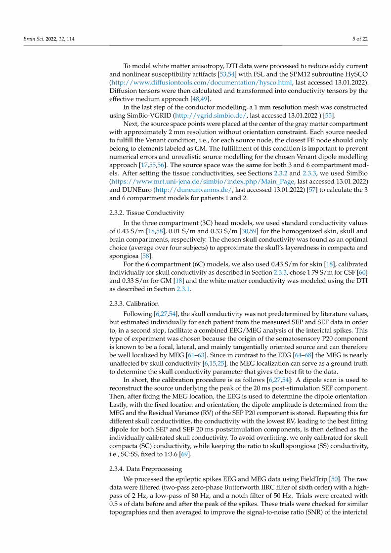
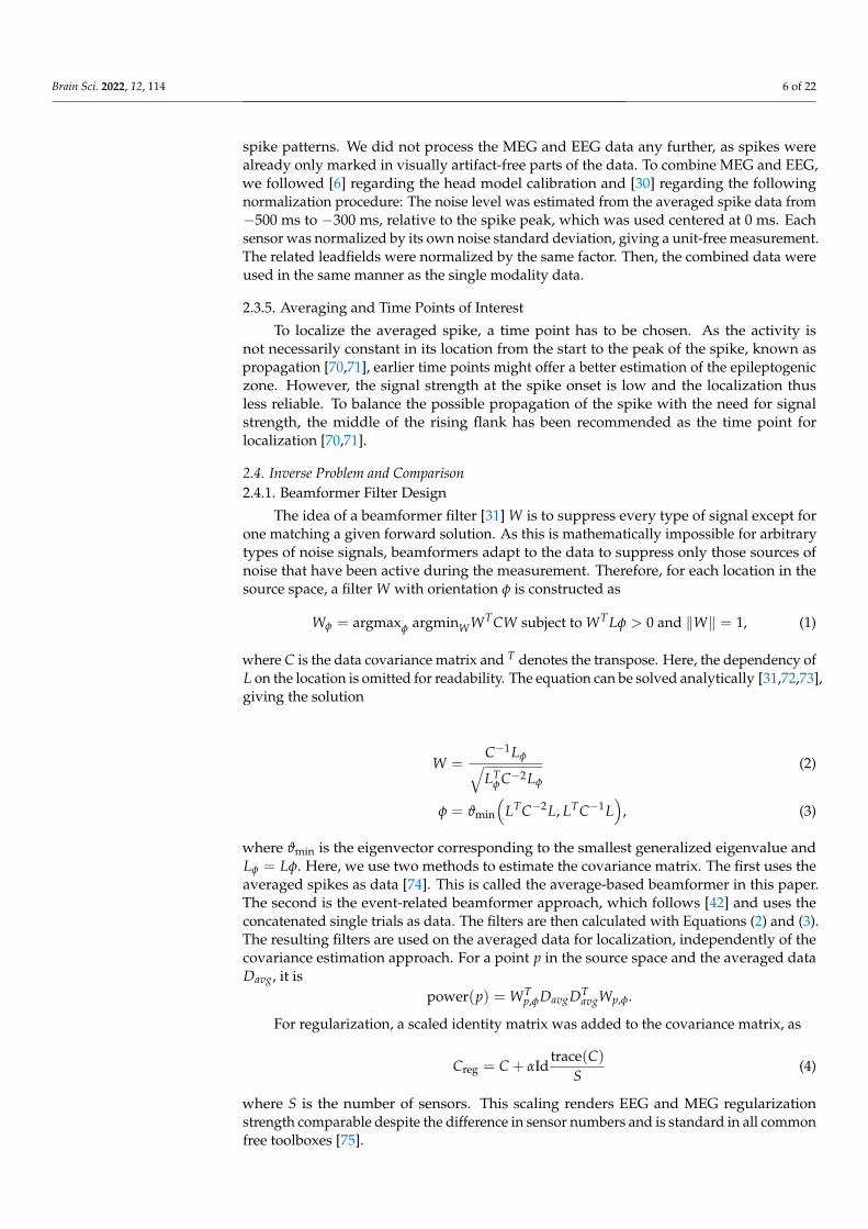
The calibrated skull compacta (SC) conductivity was determined as 0.0167 S/m for pa-tient 1. We averaged 248 spikes. The middle of the rising flank was at−6.6 ms. The butterflyplot and topographies at that time point can be seen in Figures 1 and 2, respectively.

Brain Sci. 2022, 12, 114 8 of 22

Figure 1. Butterfly plot of the averaged spikes of patient 1 in the EEG (red), MEG (blue), and MEEG(blue and red). The time point of the rising flank at −6.6 ms is marked with a vertical line from aboveand below. The horizontal line marks the zero activity line.

-12

-10

-8

-6

-4

-2

0

2

4

6

10-6

-8

-6

-4

-2

0

2

4

6

8

10

12

10-14

Figure 2. The topographic maps of patient 1, left EEG and right MEG, show the potential and fieldamplitudes with yellow for positive and blue for negative at the sensor level relative to the mean atthe time point of the middle of the rising flank at −6.6 ms. The sensors are interpolated to a spheremodel that represents the head.

3.1.1. EEG

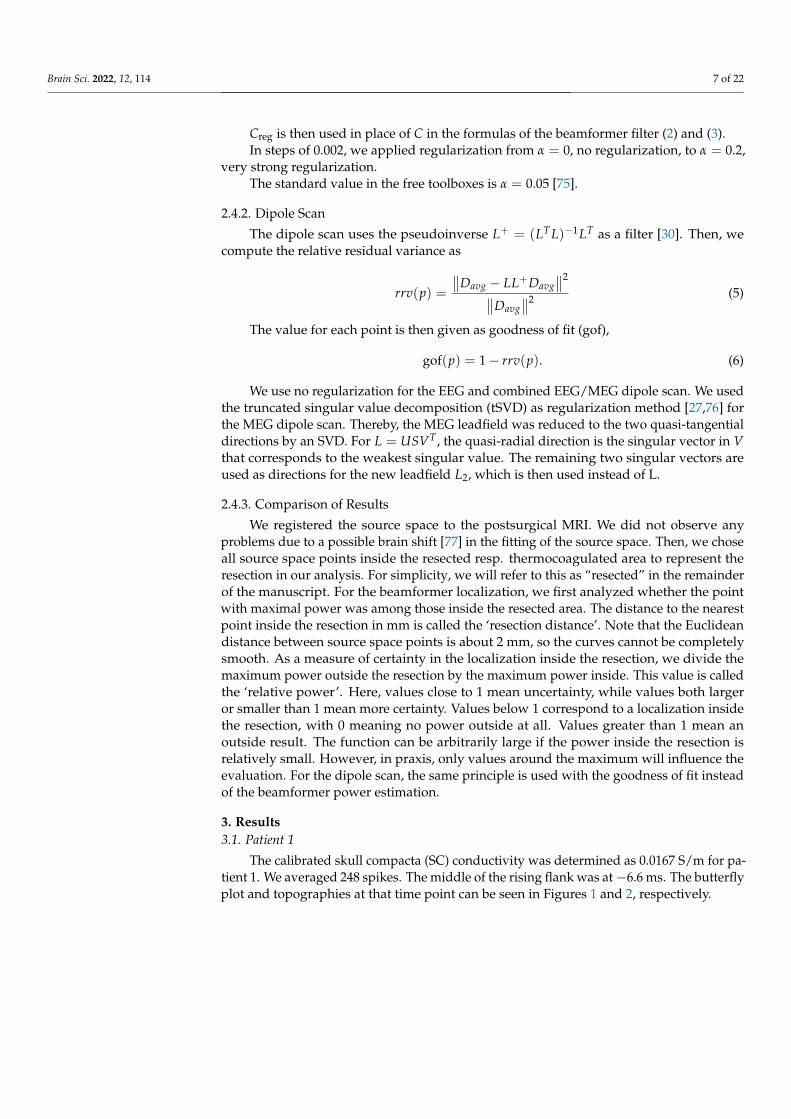
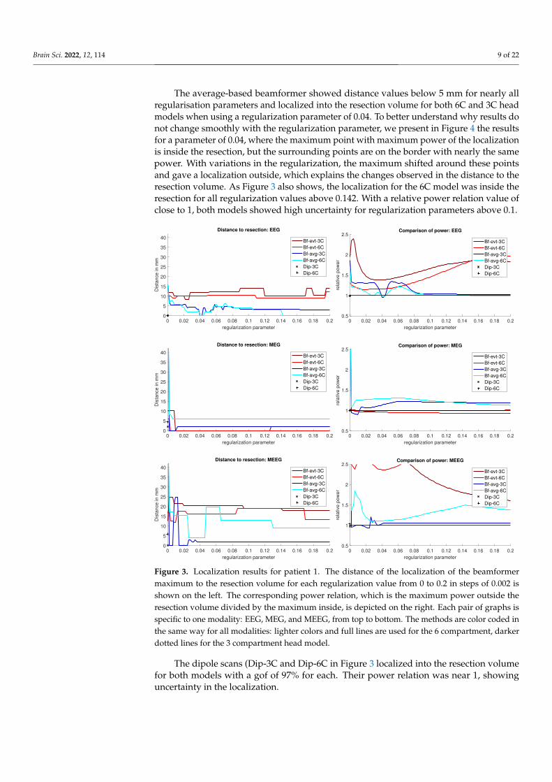
The results for Patient 1 are shown in Figure 3. It should be noted that jumps in thedistance measure do not mean large differences in the localization distribution. The beam-former power is not focused on a single spot, but positions with nearly the same power aredistributed around it, see Figure 4 or Figure 5, for an example. With changing regulariza-tion, these points are weighted differently and the maximum can shift from one to another,leading to a jump in the distance to the resection. There were overall rather low distancesfor the EEG.

The event-related beamformer behaved similarly for both the 3C and 6C head models,with a distance to the resection volume between 8 mm and 14 mm for every regularizationstrength and a maximal difference of 5 mm between 6C and 3C. The 6C beamformer’sdistance to the resection volume was overall about 2 mm lower and less affected byregularization. The relative power was high for both models, giving them a rather certainlocalization outside the resection.

Brain Sci. 2022, 12, 114 9 of 22

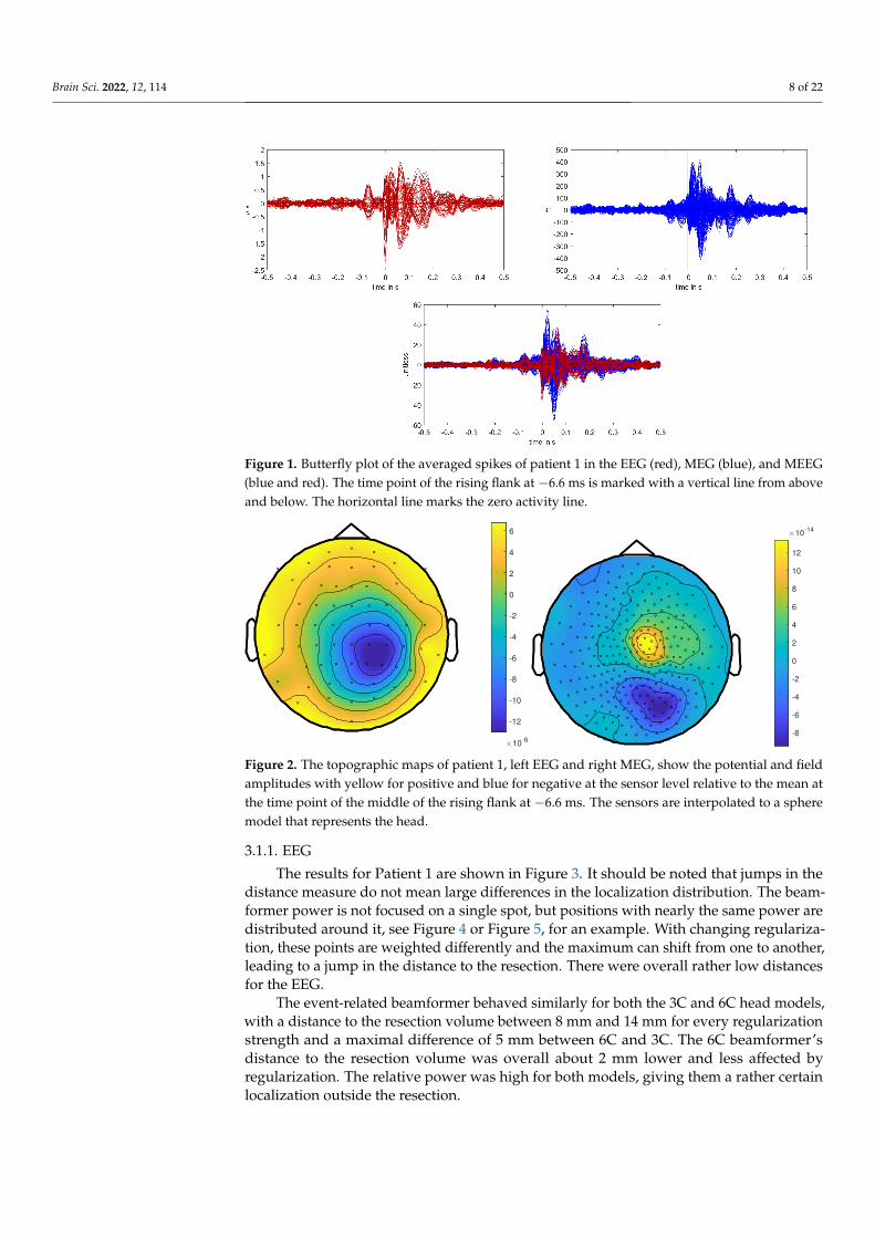
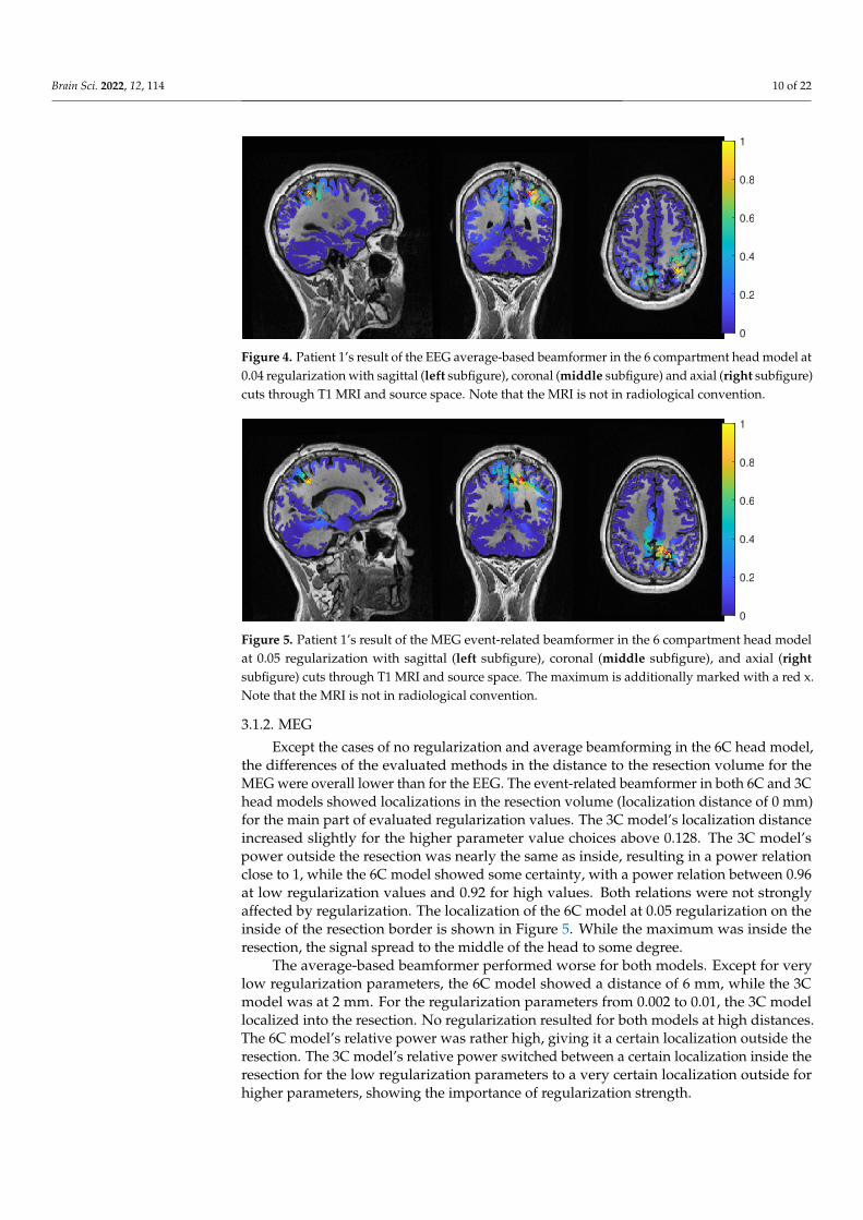
The average-based beamformer showed distance values below 5 mm for nearly allregularisation parameters and localized into the resection volume for both 6C and 3C headmodels when using a regularization parameter of 0.04. To better understand why results donot change smoothly with the regularization parameter, we present in Figure 4 the resultsfor a parameter of 0.04, where the maximum point with maximum power of the localizationis inside the resection, but the surrounding points are on the border with nearly the samepower. With variations in the regularization, the maximum shifted around these pointsand gave a localization outside, which explains the changes observed in the distance to theresection volume. As Figure 3 also shows, the localization for the 6C model was inside theresection for all regularization values above 0.142. With a relative power relation value ofclose to 1, both models showed high uncertainty for regularization parameters above 0.1.

0 0.02 0.04 0.06 0.08 0.1 0.12 0.14 0.16 0.18 0.2

regularization parameter

0

5

10

15

20

25

30

35

40

Dis

tan

ce

in

mm

Distance to resection: EEG

Bf-evt-3C

Bf-evt-6C

Bf-avg-3C

Bf-avg-6C

Dip-3C

Dip-6C

0 0.02 0.04 0.06 0.08 0.1 0.12 0.14 0.16 0.18 0.2

regularization parameter

0.5

1

1.5

2

2.5

rela

tive p

ow

er

Comparison of power: EEG

Bf-evt-3C

Bf-evt-6C

Bf-avg-3C

Bf-avg-6C

Dip-3C

Dip-6C

0 0.02 0.04 0.06 0.08 0.1 0.12 0.14 0.16 0.18 0.2

regularization parameter

0

5

10

15

20

25

30

35

40

Dis

tan

ce

in

mm

Distance to resection: MEG

Bf-evt-3C

Bf-evt-6C

Bf-avg-3C

Bf-avg-6C

Dip-3C

Dip-6C

0 0.02 0.04 0.06 0.08 0.1 0.12 0.14 0.16 0.18 0.2

regularization parameter

0.5

1

1.5

2

2.5

rela

tive p

ow

er

Comparison of power: MEG

Bf-evt-3C

Bf-evt-6C

Bf-avg-3C

Bf-avg-6C

Dip-3C

Dip-6C

0 0.02 0.04 0.06 0.08 0.1 0.12 0.14 0.16 0.18 0.2

regularization parameter

0

5

10

15

20

25

30

35

40

Dis

tan

ce

in

mm

Distance to resection: MEEG

Bf-evt-3C

Bf-evt-6C

Bf-avg-3C

Bf-avg-6C

Dip-3C

Dip-6C

0 0.02 0.04 0.06 0.08 0.1 0.12 0.14 0.16 0.18 0.2

regularization parameter

0.5

1

1.5

2

2.5

rela

tive p

ow

er

Comparison of power: MEEG

Bf-evt-3C

Bf-evt-6C

Bf-avg-3C

Bf-avg-6C

Dip-3C

Dip-6C

Figure 3. Localization results for patient 1. The distance of the localization of the beamformermaximum to the resection volume for each regularization value from 0 to 0.2 in steps of 0.002 isshown on the left. The corresponding power relation, which is the maximum power outside theresection volume divided by the maximum inside, is depicted on the right. Each pair of graphs isspecific to one modality: EEG, MEG, and MEEG, from top to bottom. The methods are color coded inthe same way for all modalities: lighter colors and full lines are used for the 6 compartment, darkerdotted lines for the 3 compartment head model.

The dipole scans (Dip-3C and Dip-6C in Figure 3 localized into the resection volumefor both models with a gof of 97% for each. Their power relation was near 1, showinguncertainty in the localization.

Brain Sci. 2022, 12, 114 10 of 22

0

0.2

0.4

0.6

0.8

1

Figure 4. Patient 1’s result of the EEG average-based beamformer in the 6 compartment head model at0.04 regularization with sagittal (left subfigure), coronal (middle subfigure) and axial (right subfigure)cuts through T1 MRI and source space. Note that the MRI is not in radiological convention.

0

0.2

0.4

0.6

0.8

1

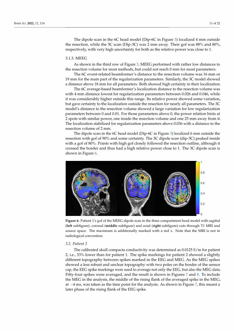
Figure 5. Patient 1’s result of the MEG event-related beamformer in the 6 compartment head modelat 0.05 regularization with sagittal (left subfigure), coronal (middle subfigure), and axial (rightsubfigure) cuts through T1 MRI and source space. The maximum is additionally marked with a red x.Note that the MRI is not in radiological convention.

3.1.2. MEG

Except the cases of no regularization and average beamforming in the 6C head model,the differences of the evaluated methods in the distance to the resection volume for theMEG were overall lower than for the EEG. The event-related beamformer in both 6C and 3Chead models showed localizations in the resection volume (localization distance of 0 mm)for the main part of evaluated regularization values. The 3C model’s localization distanceincreased slightly for the higher parameter value choices above 0.128. The 3C model’spower outside the resection was nearly the same as inside, resulting in a power relationclose to 1, while the 6C model showed some certainty, with a power relation between 0.96at low regularization values and 0.92 for high values. Both relations were not stronglyaffected by regularization. The localization of the 6C model at 0.05 regularization on theinside of the resection border is shown in Figure 5. While the maximum was inside theresection, the signal spread to the middle of the head to some degree.

The average-based beamformer performed worse for both models. Except for verylow regularization parameters, the 6C model showed a distance of 6 mm, while the 3Cmodel was at 2 mm. For the regularization parameters from 0.002 to 0.01, the 3C modellocalized into the resection. No regularization resulted for both models at high distances.The 6C model’s relative power was rather high, giving it a certain localization outside theresection. The 3C model’s relative power switched between a certain localization inside theresection for the low regularization parameters to a very certain localization outside forhigher parameters, showing the importance of regularization strength.

Brain Sci. 2022, 12, 114 11 of 22

The dipole scan in the 6C head model (Dip-6C in Figure 3) localized 4 mm outsidethe resection, while the 3C scan (Dip-3C) was 2 mm away. Their gof was 88% and 80%,respectively, with very high uncertainty for both as the relative power was close to 1.

3.1.3. MEEG

As shown in the third row of Figure 3, MEEG performed with rather low distances tothe resection volume for most methods, but could not reach 0 mm for most parameters.

The 6C event-related beamformer’s distance to the resection volume was 16 mm or19 mm for the main part of the regularization parameters. Similarly, the 3C model showeda distance above 18 mm for all parameters. Both showed high certainty in their localization.

The 6C average-based beamformer’s localization distance to the resection volume waswith 4 mm distance lowest for regularization parameters between 0.026 and 0.046, whileit was considerably higher outside this range. Its relative power showed some variation,but gave certainty to the localization outside the resection for nearly all parameters. The 3Cmodel’s distance to the resection volume showed a large variation for low regularizationparameters between 0 and 0.01. For those parameters above 0, the power relation hints at2 spots with similar power, one inside the resection volume and one 25 mm away from it.The localization stabilized for regularization parameters above 0.036 with a distance to theresection volume of 2 mm.

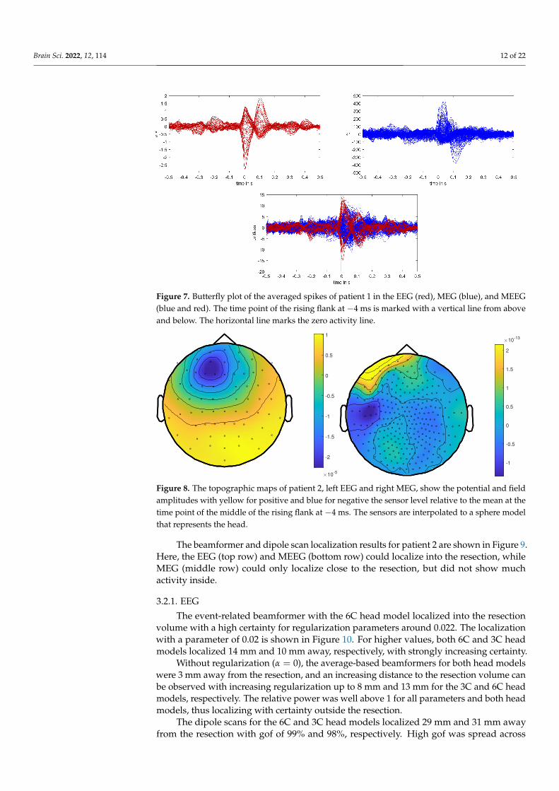
The dipole scan in the 6C head model (Dip-6C in Figure 3) localized 6 mm outside theresection with gof of 90% and some certainty. The 3C dipole scan (dip-3C) peaked insidewith a gof of 80%. Points with high gof closely followed the resection outline, although itcrossed the border and thus had a high relative power close to 1. The 3C dipole scan isshown in Figure 6.

0

0.2

0.4

0.6

0.8

1

Figure 6. Patient 1’s gof of the MEEG dipole scan in the three compartment head model with sagittal(left subfigure), coronal (middle subfigure) and axial (right subfigure) cuts through T1 MRI andsource space. The maximum is additionally marked with a red x. Note that the MRI is not inradiological convention.

3.2. Patient 2

The calibrated skull compacta conductivity was determined as 0.0125 S/m for patient2, i.e., 33% lower than for patient 1. The spike markings for patient 2 showed a slightlydifferent topography between spikes marked in the EEG and MEG. As the MEG spikesshowed a less robust and unclear topography with two poles on the border of the sensorcap, the EEG spike markings were used to average not only the EEG, but also the MEG data.Fifty-four spikes were averaged, and the result is shown in Figures 7 and 8. To includethe MEG in the analysis, the middle of the rising flank of the averaged spike in the MEG,at −4 ms, was taken as the time point for the analysis. As shown in Figure 7, this meant alater phase of the rising flank of the EEG spike.

Brain Sci. 2022, 12, 114 12 of 22

Figure 7. Butterfly plot of the averaged spikes of patient 1 in the EEG (red), MEG (blue), and MEEG(blue and red). The time point of the rising flank at −4 ms is marked with a vertical line from aboveand below. The horizontal line marks the zero activity line.

-2

-1.5

-1

-0.5

0

0.5

1

10-5

-1

-0.5

0

0.5

1

1.5

2

10-13

Figure 8. The topographic maps of patient 2, left EEG and right MEG, show the potential and fieldamplitudes with yellow for positive and blue for negative the sensor level relative to the mean at thetime point of the middle of the rising flank at −4 ms. The sensors are interpolated to a sphere modelthat represents the head.

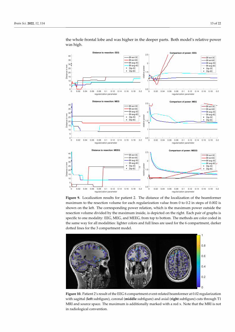
The beamformer and dipole scan localization results for patient 2 are shown in Figure 9.Here, the EEG (top row) and MEEG (bottom row) could localize into the resection, whileMEG (middle row) could only localize close to the resection, but did not show muchactivity inside.

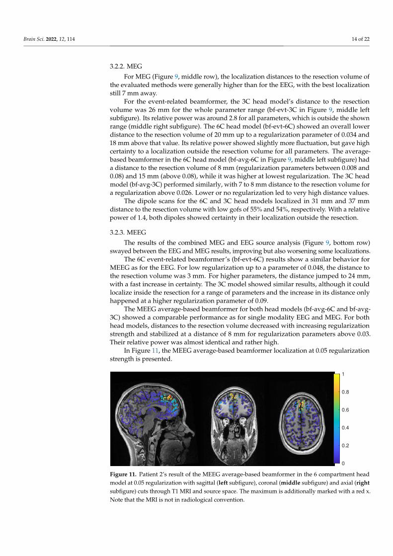
3.2.1. EEG

The event-related beamformer with the 6C head model localized into the resectionvolume with a high certainty for regularization parameters around 0.022. The localizationwith a parameter of 0.02 is shown in Figure 10. For higher values, both 6C and 3C headmodels localized 14 mm and 10 mm away, respectively, with strongly increasing certainty.

Without regularization (α = 0), the average-based beamformers for both head modelswere 3 mm away from the resection, and an increasing distance to the resection volume canbe observed with increasing regularization up to 8 mm and 13 mm for the 3C and 6C headmodels, respectively. The relative power was well above 1 for all parameters and both headmodels, thus localizing with certainty outside the resection.

The dipole scans for the 6C and 3C head models localized 29 mm and 31 mm awayfrom the resection with gof of 99% and 98%, respectively. High gof was spread across

Brain Sci. 2022, 12, 114 13 of 22

the whole frontal lobe and was higher in the deeper parts. Both model’s relative powerwas high.

0 0.02 0.04 0.06 0.08 0.1 0.12 0.14 0.16 0.18 0.2

regularization parameter

0

5

10

15

20

25

30

35

40

Dis

tan

ce

in

mm

Distance to resection: EEG

Bf-evt-3C

Bf-evt-6C

Bf-avg-3C

Bf-avg-6C

Dip-3C

Dip-6C

0 0.02 0.04 0.06 0.08 0.1 0.12 0.14 0.16 0.18 0.2

regularization parameter

0.5

1

1.5

2

2.5

rela

tive p

ow

er

Comparison of power: EEG

Bf-evt-3C

Bf-evt-6C

Bf-avg-3C

Bf-avg-6C

Dip-3C

Dip-6C

0 0.02 0.04 0.06 0.08 0.1 0.12 0.14 0.16 0.18 0.2

regularization parameter

0

5

10

15

20

25

30

35

40

Dis

tan

ce

in

mm

Distance to resection: MEG

Bf-evt-3C

Bf-evt-6C

Bf-avg-3C

Bf-avg-6C

Dip-3C

Dip-6C

0 0.02 0.04 0.06 0.08 0.1 0.12 0.14 0.16 0.18 0.2

regularization parameter

0.5

1

1.5

2

2.5

rela

tive p

ow

er

Comparison of power: MEG

Bf-evt-3C

Bf-evt-6C

Bf-avg-3C

Bf-avg-6C

Dip-3C

Dip-6C

0 0.02 0.04 0.06 0.08 0.1 0.12 0.14 0.16 0.18 0.2

regularization parameter

0

5

10

15

20

25

30

35

40

Dis

tan

ce

in

mm

Distance to resection: MEEG

Bf-evt-3C

Bf-evt-6C

Bf-avg-3C

Bf-avg-6C

Dip-3C

Dip-6C

0 0.02 0.04 0.06 0.08 0.1 0.12 0.14 0.16 0.18 0.2

regularization parameter

0.5

1

1.5

2

2.5

rela

tive p

ow

er

Comparison of power: MEEG

Bf-evt-3C

Bf-evt-6C

Bf-avg-3C

Bf-avg-6C

Dip-3C

Dip-6C

Figure 9. Localization results for patient 2. The distance of the localization of the beamformermaximum to the resection volume for each regularization value from 0 to 0.2 in steps of 0.002 isshown on the left. The corresponding power relation, which is the maximum power outside theresection volume divided by the maximum inside, is depicted on the right. Each pair of graphs isspecific to one modality: EEG, MEG, and MEEG, from top to bottom. The methods are color coded inthe same way for all modalities: lighter colors and full lines are used for the 6 compartment, darkerdotted lines for the 3 compartment model.

0

0.2

0.4

0.6

0.8

1

Figure 10. Patient 2’s result of the EEG 6 compartment event-related beamformer at 0.02 regularizationwith sagittal (left subfigure), coronal (middle subfigure) and axial (right subfigure) cuts through T1MRI and source space. The maximum is additionally marked with a red x. Note that the MRI is notin radiological convention.

Brain Sci. 2022, 12, 114 14 of 22

3.2.2. MEG

For MEG (Figure 9, middle row), the localization distances to the resection volume ofthe evaluated methods were generally higher than for the EEG, with the best localizationstill 7 mm away.

For the event-related beamformer, the 3C head model’s distance to the resectionvolume was 26 mm for the whole parameter range (bf-evt-3C in Figure 9, middle leftsubfigure). Its relative power was around 2.8 for all parameters, which is outside the shownrange (middle right subfigure). The 6C head model (bf-evt-6C) showed an overall lowerdistance to the resection volume of 20 mm up to a regularization parameter of 0.034 and18 mm above that value. Its relative power showed slightly more fluctuation, but gave highcertainty to a localization outside the resection volume for all parameters. The average-based beamformer in the 6C head model (bf-avg-6C in Figure 9, middle left subfigure) hada distance to the resection volume of 8 mm (regularization parameters between 0.008 and0.08) and 15 mm (above 0.08), while it was higher at lowest regularization. The 3C headmodel (bf-avg-3C) performed similarly, with 7 to 8 mm distance to the resection volume fora regularization above 0.026. Lower or no regularization led to very high distance values.

The dipole scans for the 6C and 3C head models localized in 31 mm and 37 mmdistance to the resection volume with low gofs of 55% and 54%, respectively. With a relativepower of 1.4, both dipoles showed certainty in their localization outside the resection.

3.2.3. MEEG

The results of the combined MEG and EEG source analysis (Figure 9, bottom row)swayed between the EEG and MEG results, improving but also worsening some localizations.

The 6C event-related beamformer’s (bf-evt-6C) results show a similar behavior forMEEG as for the EEG. For low regularization up to a parameter of 0.048, the distance tothe resection volume was 3 mm. For higher parameters, the distance jumped to 24 mm,with a fast increase in certainty. The 3C model showed similar results, although it couldlocalize inside the resection for a range of parameters and the increase in its distance onlyhappened at a higher regularization parameter of 0.09.

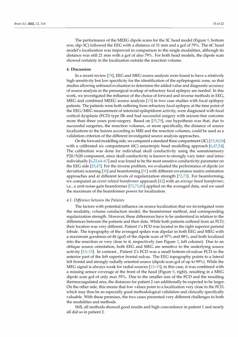
The MEEG average-based beamformer for both head models (bf-avg-6C and bf-avg-3C) showed a comparable performance as for single modality EEG and MEG. For bothhead models, distances to the resection volume decreased with increasing regularizationstrength and stabilized at a distance of 8 mm for regularization parameters above 0.03.Their relative power was almost identical and rather high.

In Figure 11, the MEEG average-based beamformer localization at 0.05 regularizationstrength is presented.

0

0.2

0.4

0.6

0.8

1

Figure 11. Patient 2’s result of the MEEG average-based beamformer in the 6 compartment headmodel at 0.05 regularization with sagittal (left subfigure), coronal (middle subfigure) and axial (rightsubfigure) cuts through T1 MRI and source space. The maximum is additionally marked with a red x.Note that the MRI is not in radiological convention.

Brain Sci. 2022, 12, 114 15 of 22

The performance of the MEEG dipole scans for the 3C head model (Figure 9, bottomrow, dip-3C) followed the EEG with a distance of 31 mm and a gof of 79%. The 6C headmodel’s localization was improved in comparison to the single modalities, although itsdistance was still 21 mm with a gof of also 79%. For both head models, the dipole scanshowed certainty in the localization outside the resection volume.

4. Discussion

In a recent review [78], EEG and MEG source analysis were found to have a relativelyhigh sensitivity but low specificity for the identification of the epileptogenic zone, so thatstudies allowing unbiased evaluation to determine the added value and diagnostic accuracyof source analysis in the presurgical workup of refractory focal epilepsy are needed. In thiswork, we investigated the influence of the choice of forward and inverse methods in EEG,MEG and combined MEEG source analysis [15] in two case studies with focal epilepsypatients. The patients were both suffering from refractory focal epilepsy at the time point ofthe EEG/MEG measurement of interictal epileptiform activity, were diagnosed with focalcortical dysplasia (FCD) type IIb and had successful surgery with seizure-free outcomemore than three years post-surgery. Based on [35,79], our hypothesis was that, due tosuccessful surgeries, the resection volumes, or more specifically, the distance of sourcelocalizations to the lesions according to MRI and the resection volumes, could be used as avalidation criterion of the different investigated source analysis approaches.

On the forward modelling side, we compared a standard three compartment (3C) [15,30,54]with a calibrated six compartment (6C) anisotropic head modelling approach [6,47,54].The calibration was done for individual skull conductivity using the somatosensoryP20/N20 component, since skull conductivity is known to strongly vary inter- and intra-individually [6,22,64–67] and was found to be the most sensitive conductivity parameter onthe EEG side [25,47]. For the inverse problem, we evaluated the performance of dipole (ordeviation) scanning [30] and beamforming [31] with different covariance matrix estimationapproaches and at different levels of regularization strength [72,73]. For beamforming,we compared an event-related beamformer approach [42] with an average based beamformer,i.e., a unit-noise-gain beamformer [72,73,80] applied on the averaged data, and we usedthe maximum of the beamformer power for localization.

4.1. Difference between the Patients

The factors with potential influence on source localization that we investigated werethe modality, volume conduction model, the beamformer method, and correspondingregularization strength. However, these differences have to be understood in relation to thedifferences between the patients and their data. While both patients suffered from an FCD,their location was very different. Patient 1’s FCD was located in the right superior parietallobule. The topography of the averaged spikes was dipolar in both EEG and MEG witha maximum goodness-of-fit (gof) of the dipole scan of 97% and 88%, and both localizedinto the resection or very close to it, respectively (see Figure 3, left column). Due to anoblique source orientation, both EEG and MEG are sensitive to the underlying sourceactivity [13–15]. In contrast , Patient 2’s FCD was a small bottom-of-sulcus FCD in theanterior part of the left superior frontal sulcus. The EEG topography points to a lateralleft frontal and strongly radially oriented source (dipole scan gof of up to 99%). While theMEG signal is always weak for radial sources [13–15], in this case, it was combined witha missing sensor coverage at the front of the head (Figure 8, right), resulting in a MEGdipole scan gof of only max 55%. Due to the smaller size of the FCD and the resultingthermocoagulated area, the distances for patient 2 can additionally be expected to be larger.On the other side, this means that low values point to a localization very close to the FCD,which may thus be an especially good methodological validation and clinically specificallyvaluable. With these premises, the two cases presented very different challenges to boththe modalities and methods.

Still, all methods showed good results and high concordance in patient 1 and nearlyall did so in patient 2.

Brain Sci. 2022, 12, 114 16 of 22

4.2. Beamformer Parameters and Localization

In contrast to the dipole scan, beamformers can localize ongoing activity and are notdependent on time-locked data. However, they profit from high SNR and thus averaging,when appropriate. For epileptic spikes, clustering of single spike localization might showvaluable information about the extent of the irritative zone [71,81,82], but averaging of sim-ilar spikes increases the SNR and improves the reliability of the reconstruction [71,83,84].In our study, we try to localize the center of gravity of the spike activity, which is easierto compare to the standard dipole scan approach. Both beamformer methods we inves-tigated try to optimize the beamformer design to event data, but differ in the estimationof the covariance matrix. The average-based beamformer is a straight application of thebeamformer approach [85] on the averaged data and has been shown by [74] to give sim-ilar results to dipole scans on fields evoked by median nerve stimulation. By using theconcatenated single trials instead of the averaged data for the estimation of the covariancematrix, the event-related beamformer [41,42] approach offers a more flexible approach. Itcan be used with events that are time-locked and those that evoke a synchronization. Itwas first introduced by [41] for motor tasks and has been used successfully for epilepsydata [86]. Increasing the time sample size should improve the covariance estimation [40]and decrease the need for regularization [40–42]. However, the SNR of the single trials willbe lower, and the covariance matrix might include noise components that would have beenremoved by averaging first [41,42]. In our investigation, neither approach showed a clearadvantage. While we see a tendency for the average-based approach to be more stableacross modalities, it did not necessarily localize closer to the resection (see left column inFigures 3 and 9). For both MEG and MEEG, using no regularization resulted in high dis-tances for the average-based approach, while the event-related approach had much smallervariations at low regularization strength, which seems to confirm the ideas of [41,42].For higher strength, both methods showed a similar behavior, with usually low changes inthe distance to the resection, although some jumps of 1 cm to 2 cm have appeared, mostlyin the MEEG. This seems to indicate that the scaling [75], shown in Equation (4), worksas intended. In the two cases, the optimal regularization strength was lower than thequasi standard of 0.05 [75], which is used by all open source toolboxes. For all modalities,parameter values in the range of 0.02 to 0.04 performed better, even though 0.05 wouldhave still given good results (Figures 3 and 9). Overall, we can onlyrecommend applyingsome regularization, especially with the average-based approach, and to report on thevalues used.

Except for the estimation of the covariance, we used the same filter design for bothapproaches. As the linear constraint of the filter introduces a depth bias, the depth nor-malization by the filter norm or a noise covariance matrix was introduced, called ‘neuralactivity index’ [85] or ‘Pseudo-Z value’ [87]. The unit-noise gain filter that we used givesan analytical formulation of a filter with the same output, but in a single step [72]. Thisenables the derivation of an optimal source direction, which increases output SNR and isfast to compute [72].

In comparison to the dipole scan, the beamformer showed comparable accuracy forpatient 1 and better results for patient 2. Our findings in the examined two patients are con-cordant with [86], showing that beamformers are a reliable way to localize epileptic spikes.

4.3. Models and Modalities

We compared the performance of a three compartment and a six compartment modelwith the same source space. In most cases, neither model had a significant advantageto the other and better performance in one case was offset with worse performance inanother. Often, the models showed a shifted behavior, with the same tendencies at higheror lower regularization.

From single dipolar source simulations, differences from a few millimeters to centime-ters have to be expected between 3C and 6C models [17,80], which fits to our results withdifferences from millimeter range to maximally 2.5 cm (event-related MEEG beamformer

Brain Sci. 2022, 12, 114 17 of 22

in Figure 9). Ref. [88] found accurate skull modelling to be necessary for EEG sourcemodelling, with especially high errors near suture line. Since we investigated only thedistance to the resection and not between the foci of the methods, these distances cannotbe precisely inferred. For example, the EEG dipole scan for patient 1 localized into theresection volume for both models, but did not localize the same position. Furthermore,we only evaluated localization and not the source orientation and strength differences,which are known to be considerably influenced by volume conduction differences betweenisotropic 3C and anisotropic 6C models [6,17,24,25]. Source orientation, for example, mightalso be important in addition to absolute localization in attributing epileptic activity tosubcompartments of the respective brain area [49,89,90].

In both patients, the calibrated skull conductivity in the 6 compartment model,i.e., 0.0167 S/m for patient 1 and 0.0125 S/m for patient 2, was relatively close to thestandard value of 0.01 S/m used in the 3 compartment model. This helps to explain whythe localization differences between the 3C and 6C models were often only in the millimeterrange, when knowing that skull conductivity is the most sensitive conductivity param-eter for the EEG source localization [25,64,65]. It should be noted here that this relationis specific to these patients and should not be generalized, as calibrated skull compactaconductivity values of 0.0033 S/m [91] and 0.0024 S/m [54] and an age-dependency with,however, a large interindividual variability [6], have been found.

Our source space was limited to the gray matter surface for both 6C and 3C headmodels, which is also useful to improve the realism of the reconstruction, since EEG andMEG dipolar sources can only be found in the gray matter compartment [15]. For the orien-tation of the sources, we used no constraints. While the sources should be perpendicularto the cortex surface, at least in a healthy brain [15,45,92,93], the constraint inhibits thelocalization quality when the modelling is not exact. In [94], the beamformer quality dete-riorated strongly with errors in MRI registration and the estimation of the cortex surface.Additionally, errors in the head modelling, especially conductivity modelling, will furtherinfluence the localization [80]. This is why we do not recommend a normal constraint, evenif on the other side, a dimension reduction could have a positive effect on the SNR of thebeamformer reconstruction [72,94].

Both MEG and EEG gave good results for our patients, even if, with the investigatedparameters, the MEG performance was slightly more robust to regularization. The com-bined analysis of MEG and EEG gave comparable and satisfying results with respect to theclinical outcome, further strengthening the contribution of non-invasive source analysisto presurgical epilepsy diagnosis and to guiding the positioning of sEEG or ECoG grids.With our imprecise error measure (see below) and the good results for the single modalities,a strong improvement like seen in [71,91] was unlikely. In addition, Ref. [83] reporteda strong improvement of MEG localization results of anterior temporal spikes when afew EEG electrodes were included. Our results thus further motivate combined MEEGsource analysis, while we also showed that, due to the remaining model inaccuracies,combined MEEG results should always be compared to results of single modality EEG orMEG source analysis.

4.4. Limitations of Our Error Criterion

Finally, it is surely very important to understand the limitations of our source anal-ysis validation criterion, i.e., the distance to the resection volume. In the case of FCD,the irritative zone might only be neighboring the FCD and therefore the resection volume.A reason for this might be that the pyramidal cells inside the FCD volume might not buildan open field structure, which is, however, necessary to produce activity that can be markedin EEG and MEG [45,92,93]. In such a case, a source analysis result with a considerabledistance to the resection volume might still be accurately reconstructing the irritative zone.Furthermore, the MRI correlate of an FCD IIb, which significantly influences the definitionof the resection volume, predominantly corresponds to the distribution of pathologic bal-loon cells [45,95,96], which however are electrophysiologically silent [45,97]. In contrast,dysmorphic neurons, the putative epileptogenic cell population, show an overlapping,

Brain Sci. 2022, 12, 114 18 of 22

but importantly not identical distribution [45,96]. Their MRI correlate is, however, subtle:inhomogeneities of the intracortical signal [96,98] and blurring of the gray-white matterjunction due to dyslamination [99]. Correspondingly, these discrepancies introduce furtherpotential variability between the location of the epileptogenic zone, the MRI finding andcorrespondingly the resection volume. All results in this work thus have to be seen in thelight of these limitations to our validation criterion, while on the other side there might beno better one than the use of the resection volumes in seizure-free patients.

5. Conclusions

Beamformers can be used to localize epileptic spikes. In some cases, they can out-perform dipole scans, but the real activity is hard to distinguish when the localization ofdifferent methods differ. Using the covariance of the average data gave more stable resultsthan using concatenated trials. The difference between our 3 and 6 compartment modelswere only in the millimeter to centimeter range, most probably due to very similar skullconductivity and the usage of a gray matter source space without orientation constraint.Regularization strength is an important factor, especially when only the maximum po-sition of the beamformer localization is used. While not optimal in the presented cases,the standard value of 0.05 gave good results.

Author Contributions: Conceptualization, F.N., S.R. and C.H.W.; Data curation, M.A., K.U., Y.P., J.W.,S.R. and C.H.W.; Formal analysis, F.N. and M.A.; Funding acquisition, S.R. and C.H.W.; Investigation,M.A., K.U., Y.P., J.W. and S.R.; Methodology, F.N. and M.A.; Project administration, C.H.W.; Resources,S.R. and C.H.W.; Software, F.N. and M.A.; Supervision, C.H.W.; Validation, F.N., M.A., K.U., Y.P., J.W.,S.R. and C.H.W.; Visualization, F.N.; Writing—original draft, F.N.; Writing—review and editing, S.R.and C.H.W. All authors have read and agreed to the published version of the manuscript.

Funding: This research was supported by the German Research Foundation (DFG) through projectsWO1425/7-1 and RA2062/1-1 and by the Bundesministerium für Gesundheit (BMG) as projectZMI1-2521FSB006, under the frame of ERA PerMed as project ERAPERMED2020-227 PerEpi.

Institutional Review Board Statement: The study was conducted according to the guidelines of theDeclaration of Helsinki, and approved by the ethics committee of the University of Erlangen, Facultyof Medicine on 10510.05.2011 (Ref. No. 4453).

Informed Consent Statement: Informed consent was obtained from all subjects involved in the study.

Data Availability Statement: The data are not publicly available due to patient privacy. Codes areavailable on request from the corresponding author.

Acknowledgments: We thank Andreas Wollbrink for technical assistance and Karin Wilken, Hilde-gard Deitermann, Ute Trompeter, and Harald Kugel for their help with the EEG/MEG/MRI datacollection, and Sampsa Pursiainen for good discussions.

Conflicts of Interest: The authors declare no conflict of interest.

References1. Kwan, P.; Arzimanoglou, A.; Berg, A.T.; Brodie, M.J.; Hauser, W.A.; Mathern, G.; Moshé, S.L.; Perucca, E.; Wiebe, S.; French, J.

Definition of drug resistant epilepsy: Consensus proposal by the ad hoc Task Force of the ILAE Commission on TherapeuticStrategies. Epilepsia 2010, 51, 1069–1077. [CrossRef] [PubMed]

2. Taylor, R.S.; Sander, J.W.; Taylor, R.J.; Baker, G.A. Predictors of health-related quality of life and costs in adults with epilepsy: Asystematic review. Epilepsia 2011, 52, 2168–2180. [CrossRef] [PubMed]

3. Brodie, M.J.; Barry, S.J.E.; Bamagous, G.A.; Norrie, J.D.; Kwan, P. Patterns of treatment response in newly diagnosed epilepsy.Neurology 2012, 78, 1548–1554. [CrossRef] [PubMed]

4. Blumcke, I.; Spreafico, R.; Haaker, G.; Coras, R.; Kobow, K.; Bien, C.G.; Pfäfflin, M.; Elger, C.; Widman, G.; Schramm, J.; et al.Histopathological findings in brain tissue obtained during epilepsy surgery. N. Engl. J. Med. 2017, 377, 1648–1656. [CrossRef]

5. De Tisi, J.; Bell, G.S.; Peacock, J.L.; McEvoy, A.W.; Harkness, W.F.; Sander, J.W.; Duncan, J.S. The long-term outcome of adultepilepsy surgery, patterns of seizure remission, and relapse: A cohort study. Lancet 2011, 378, 1388–1395. [CrossRef]

6. Antonakakis, M.; Schrader, S.; Aydin, Ü.; Khan, A.; Gross, J.; Zervakis, M.; Rampp, S.; Wolters, C.H. Inter-Subject Variability ofSkull Conductivity and Thickness in Calibrated Realistic Head Models. NeuroImage 2020, 223, 117353. [CrossRef]

Brain Sci. 2022, 12, 114 19 of 22

7. Ossenblok, P.; De Munck, J.C.; Colon, A.; Drolsbach, W.; Boon, P. Magnetoencephalography is more successful for screening andlocalizing frontal lobe epilepsy than electroencephalography. Epilepsia 2007, 48, 2139–2149. [CrossRef]

8. Sutherling, W.W.; Mamelak, A.N.; Thyerlei, D.; Maleeva, T.; Minazad, Y.; Philpott, L.; Lopez, N. Influence of magnetic sourceimaging for planning intracranial EEG in epilepsy. Neurology 2008, 71, 990–996. [CrossRef]

9. Murakami, H.; Wang, Z.I.; Marashly, A.; Krishnan, B.; Prayson, R.A.; Kakisaka, Y.; Mosher, J.C.; Bulacio, J.; Gonzalez-Martinez,J.A.; Bingaman, W.E.; et al. Correlating magnetoencephalography to stereo-electroencephalography in patients undergoingepilepsy surgery. Brain 2016, 139, 2935–2947. [CrossRef]

10. Stefan, H.; Hummel, C.; Scheler, G.; Genow, A.; Druschky, K.; Tilz, C.; Kaltenhäuser, M.; Hopfengärtner, R.; Buchfelder, M.;Romstöck, J. Magnetic brain source imaging of focal epileptic activity: A synopsis of 455 cases. Brain 2003, 126, 2396–2405.[CrossRef]

11. Rampp, S.; Stefan, H.; Wu, X.; Kaltenhäuser, M.; Maess, B.; Schmitt, F.C.; Wolters, C.H.; Hamer, H.; Kasper, B.S.; Schwab, S.; et al.Magnetoencephalography for epileptic focus localization in a series of 1000 cases. Brain 2019, 142, 3059–3071. [CrossRef]

12. Dassios, G.; Fokas, A.S.; Hadjiloizi, D. On the complementarity of electroencephalography and magnetoencephalography. InverseProbl. 2007, 23, 2541–2549. [CrossRef]

13. Iwasaki, M.; Pestana, E.; Burgess, R.C.; Luders, H.O.; Shamoto, H.; Nakasato, N. Detection of Epileptiform Activity by HumanInterpreters: Blinded Comparison between Electroencephalography and Magnetoencephalography. Epilepsia 2005, 46, 59–68.[CrossRef]

14. Knake, S.; Halgren, E.; Shiraishi, H.; Hara, K.; Hamer, H.; Grant, P.; Carr, V.; Foxe, D.; Camposano, S.; Busa, E.; et al. The value ofmultichannel MEG and EEG in the presurgical evaluation of 70 epilepsy patients. Epilepsy Res. 2006, 69, 80–86. [CrossRef]

15. Brette, R.; Destexhe, A. (Eds.) Handbook of Neural Activity Measurement; Cambridge University Press: Cambridge, UK, 2012.[CrossRef]

16. Montes-Restrepo, V.; Van Mierlo, P.; Strobbe, G.; Staelens, S.; Vandenberghe, S.; Hallez, H. Influence of skull modelling approacheson EEG source localization. Brain Topogr. 2014, 27, 95–111. [CrossRef]

17. Vorwerk, J.; Cho, J.H.; Rampp, S.; Hamer, H.; Knösche, T.R.; Wolters, C.H. A guideline for head volume conductor modelling inEEG and MEG. NeuroImage 2014, 100, 590–607. [CrossRef]

18. Ramon, C.; Schimpf, P.; Haueisen, J.; Holmes, M.; Ishimaru, A. Role of soft bone, CSF and gray matter in EEG simulations. BrainTopogr. 2004, 16, 245–248.:BRAT.0000032859.68959.76. [CrossRef]

19. Rice, J.K.; Rorden, C.; Little, J.S.; Parra, L.C. Subject position affects EEG magnitudes. NeuroImage 2013, 64, 476–484. [CrossRef]20. Azizollahi, H.; Aarabi, A.; Wallois, F. Effects of uncertainty in head tissue conductivity and complexity on EEG forward modelling

in neonates. Hum. Brain Mapp. 2016, 37, 3604–3622. [CrossRef]21. Piastra, M.C.; Nüßing, A.; Vorwerk, J.; Clerc, M.; Engwer, C.; Wolters, C.H. A comprehensive study on electroencephalography

and magnetoencephalography sensitivity to cortical and subcortical sources. Hum. Brain Mapp. 2021, 42, 978–992. [CrossRef]22. McCann, H.; Pisano, G.; Beltrachini, L. Variation in Reported Human Head Tissue Electrical Conductivity Values. Brain Topogr.

2019, 32, 825–858. [CrossRef]23. Hallez, H.; Vanrumste, B.; Hese, P.V.; Delputte, S.; Lemahieu, I. Dipole estimation errors due to differences in modelling

anisotropic conductivities in realistic head models for EEG source analysis. Phys. Med. Biol. 2008, 53, 1877–1894. [CrossRef]24. Güllmar, D.; Haueisen, J.; Reichenbach, J.R. Influence of anisotropic electrical conductivity in white matter tissue on the EEG/MEG

forward and inverse solution. A high-resolution whole head simulation study. NeuroImage 2010, 51, 145–163. [CrossRef]25. Vorwerk, J.; Aydin, Ü.; Wolters, C.H.; Butson, C.R. Influence of head tissue conductivity uncertainties on EEG dipole reconstruction.

Front. Neurosci. 2019, 13, 1–17. [CrossRef]26. Vallaghe, S.; Clerc, M. A Global Sensitivity Analysis of Three- and Four-Layer EEG Conductivity Models. IEEE Trans. Biomed.

Eng. 2009, 56, 988–995. [CrossRef]27. Huang, M.X.; Song, T.; Hagler, D.J.; Podgorny, I.; Jousmaki, V.; Cui, L.; Gaa, K.; Harrington, D.L.; Dale, A.M.; Lee, R.R.; et al. A

novel integrated MEG and EEG analysis method for dipolar sources. NeuroImage 2007, 37, 731–748. [CrossRef]28. Schimpf, P.; Ramon, C.; Haueisen, J. Dipole models for the EEG and MEG. IEEE Trans. Biomed. Eng. 2002, 49, 409–418. [CrossRef]29. Beltrachini, L. Sensitivity of the Projected Subtraction Approach to Mesh Degeneracies and Its Impact on the Forward Problem in

EEG. IEEE Trans. Biomed. Eng. 2019, 66, 273–282. [CrossRef]30. Fuchs, M.; Wagner, M.; Wischmann, H.A.; Köhler, T.; Theißen, A.; Drenckhahn, R.; Buchner, H. Improving source reconstructions

by combining bioelectric and biomagnetic data. Electroencephalogr. Clin. Neurophysiol. 1998, 107, 93–111. [CrossRef]31. Van Veen, B.; Van Drongelen, W.; Yuchtman, M.; Suzuki, A. Localization of brain electrical activity via linearly constrained

minimum variance spatial filtering. IEEE Trans. Biomed. Eng. 1997, 44, 867–880. [CrossRef]32. Gross, J.; Kujala, J.; Hamalainen, M.; Timmermann, L.; Schnitzler, A.; Salmelin, R. Dynamic imaging of coherent sources: Studying

neural interactions in the human brain. Proc. Natl. Acad. Sci. USA 2001, 98, 694–699. [CrossRef] [PubMed]33. Hillebrand, A.; Singh, K.D.; Holliday, I.E.; Furlong, P.L.; Barnes, G.R. A new approach to neuroimaging with magnetoencephalog-

raphy. Hum. Brain Mapp. 2005, 25, 199–211. [CrossRef] [PubMed]34. Kirsch, H.E.; Robinson, S.; Mantle, M.; Nagarajan, S. Automated localization of magnetoencephalographic interictal spikes by

adaptive spatial filtering. Clin. Neurophysiol. 2006, 117, 2264–2271. [CrossRef] [PubMed]35. Hall, M.B.; Nissen, I.A.; van Straaten, E.C.; Furlong, P.L.; Witton, C.; Foley, E.; Seri, S.; Hillebrand, A. An evaluation of kurtosis

beamforming in magnetoencephalography to localize the epileptogenic zone in drug resistant epilepsy patients. Clin. Neurophysiol.2018, 129, 1221–1229. [CrossRef]

Brain Sci. 2022, 12, 114 20 of 22

36. Velmurugan, J.; Nagarajan, S.S.; Mariyappa, N.; Ravi, S.G.; Thennarasu, K.; Mundlamuri, R.C.; Raghavendra, K.; Bharath,R.D.; Saini, J.; Arivazhagan, A.; et al. Magnetoencephalographic imaging of ictal high-frequency oscillations (80–200 Hz) inpharmacologically resistant focal epilepsy. Epilepsia 2018, 59, 190–202. [CrossRef]

37. van Klink, N.; Hillebrand, A.; Zijlmans, M. Identification of epileptic high frequency oscillations in the time domain by usingMEG beamformer-based virtual sensors. Clin. Neurophysiol. 2016, 127, 197–208. [CrossRef]

38. Nissen, I.A.; Stam, C.J.; Reijneveld, J.C.; van Straaten, I.E.C.W.; Hendriks, E.J.; Baayen, J.C.; De Witt Hamer, P.C.; Idema,S.; Hillebrand, A. Identifying the epileptogenic zone in interictal resting-state MEG source-space networks. Epilepsia 2016,58, 137–148. [CrossRef]

39. Van Dellen, E.; Douw, L.; Hillebrand, A.; de Witt Hamer, P.C.; Baayen, J.C.; Heimans, J.J.; Reijneveld, J.C.; Stam, C.J. Epilepsy surgeryoutcome and functional network alterations in. NeuroImage 2014, 86, 354–363. [CrossRef]

40. Brookes, M.J.; Vrba, J.; Robinson, S.E.; Stevenson, C.M.; Peters, A.M.A.M.; Barnes, G.R.; Hillebrand, A.; Morris, P.G. Optimisingexperimental design for MEG beamformer imaging. NeuroImage 2008, 39, 1788–1802. [CrossRef]

41. Cheyne, D.O.; Bakhtazad, L.; Gaetz, W. Spatiotemporal mapping of cortical activity accompanying voluntary movements usingan event-related beamforming approach. Hum. Brain Mapp. 2006, 27, 213–229. [CrossRef]

42. Cheyne, D.; Bostan, A.C.; Gaetz, W.; Pang, E.W. Event-related beamforming: A robust method for presurgical functional mappingusing MEG. Clin. Neurophysiol. 2007, 118, 1691–1704. [CrossRef] [PubMed]

43. Rosenow, F.; Lüders, H. Presurgical evaluation of epilepsy. Brain 2001, 124, 1683–700. [CrossRef] [PubMed]44. Zucca, I.; Milesi, G.; Padelli, F.; Rossini, L.; Gozzo, F.; Figini, M.; Barbaglia, A.; Cardinale, F.; Tassi, L.; Bruzzone, M.G.; et al. An

image registration protocol to integrate electrophysiology, MRI and neuropathology data in epileptic patients explored withintracerebral electrodes. J. Neurosci. Methods 2018, 303, 159–168. [CrossRef] [PubMed]

45. Rampp, S.; Rössler, K.; Hamer, H.; Illek, M.; Buchfelder, M.; Doerfler, A.; Pieper, T.; Hartlieb, T.; Kudernatsch, M.; Koelble, K.; et al.Dysmorphic neurons as cellular source for phase-amplitude coupling in Focal Cortical Dysplasia Type II. Clin. Neurophysiol. 2021,132, 782–792. [CrossRef]

46. Wellmer, J.; Parpaley, Y.; Rampp, S.; Popkirov, S.; Kugel, H.; Aydin, Ü.; Wolters, C.H.; von Lehe, M.; Voges, J. Lesion guidedstereotactic radiofrequency thermocoagulation for palliative, in selected cases curative epilepsy surgery. Epilepsy Res. 2016,121, 39–46. [CrossRef]

47. Schrader, S.; Antonakakis, M.; Rampp, S.; Engwer, C.; Wolters, C.H. A novel method for calibrating head models to account forvariability in conductivity and its evaluation in a sphere model. Phys. Med. Biol. 2020, 65, 1–22. [CrossRef]

48. Tuch, D.S.; Wedeen, V.J.; Dale, A.M.; George, J.S.; Belliveau, J.W. Conductivity tensor mapping of the human brain using diffusiontensor MRI. Proc. Natl. Acad. Sci. USA 2001, 98, 11697–11701. [CrossRef]

49. Rullmann, M.; Anwander, A.; Dannhauer, M.; Warfield, S.K.; Duffy, F.H.; Wolters, C.H. EEG source analysis of epileptiformactivity using a 1 mm anisotropic hexahedra finite element head model. NeuroImage 2009, 44, 399–410. [CrossRef]

50. Oostenveld, R.; Fries, P.; Maris, E.; Schoffelen, J.M. FieldTrip: Open source software for advanced analysis of MEG, EEG, andinvasive electrophysiological data. Comput. Intell. Neurosci. 2011, 2011, 156869. [CrossRef]

51. Otsu, N. A Threshold Selection Method from Gray-Level Histograms. IEEE Trans. Syst. Man Cybern. 1979, 20, 62–66. [CrossRef]52. Lanfer, B.; Scherg, M.; Dannhauer, M.; Knösche, T.R.; Wolters, C.H. Influences of Skull Segmentation Deficiencies on EEG Source

Analysis. NeuroImage 2012, 62, 418–431. [CrossRef]53. Ruthotto, L.; Kugel, H.; Olesch, J.; Fischer, B.; Modersitzki, J.; Burger, M.; Wolters, C.H. Diffeomorphic susceptibility artifact

correction of diffusion-weighted magnetic resonance images. Phys. Med. Biol. 2012, 57, 5715–5731. [CrossRef]54. Aydin, Ü.; Vorwerk, J.; Küpper, P.; Heers, M.; Kugel, H.; Galka, A.; Hamid, L.; Wellmer, J.; Kellinghaus, C.; Rampp, S.; Wolters,

C.H. Combining EEG and MEG for the Reconstruction of Epileptic Activity Using a Calibrated Realistic Volume ConductorModel. PLoS ONE 2014, 9, e93154. [CrossRef]

55. Wolters, C.H.; Anwander, A.; Berti, G.; Hartmann, U. Geometry-Adapted Hexahedral Meshes Improve Accuracy of Finite-Element-Method-Based EEG Source Analysis. IEEE Trans. Biomed. Eng. 2007, 54, 1446–1453. [CrossRef]

56. Medani, T.; Lautru, D.; Schwartz, D.; Ren, Z.; Sou, G. FEM method for the EEG forward problem and improvement based onmodification of the Saint Venant’s method. Prog. Electromagn. Res. 2015, 153, 11–22. [CrossRef]

57. Schrader, S.; Westhoff, A.; Piastra, M.C.; Miinalainen, T.; Pursiainen, S.; Vorwerk, J.; Brinck, H.; Wolters, C.H.; Engwer, C.DUNEuro—A software toolbox for forward modelling in bioelectromagnetism. PLoS ONE 2021, 16, e0252431. [CrossRef]

58. Dannhauer, M.; Lanfer, B.; Wolters, C.H.; Knösche, T.R. Modeling of the human skull in EEG source analysis. Hum. Brain Mapp.2011, 32, 1383–1399. [CrossRef]

59. Homma, S.; Musha, T.; Nakajima, Y.; Okamoto, Y.; Blom, S.; Flink, R.; Hagbarth, K.E. Conductivity ratios of the scalp-skull-brainhead model in estimating equivalent dipole sources in human brain. Neurosci. Res. 1995, 22, 51–55. [CrossRef]

60. Baumann, S.B.; Wozny, D.R.; Kelly, S.K.; Meno, F.M. The electrical conductivity of human cerebrospinal fluid at body temperature.IEEE Trans. Biomed. Eng. 1997, 44, 220–225. [CrossRef]

61. Hari, R.; Karhu, J.; Hämäläinen, M.; Knuutila, J.; Salonen, O.; Sams, M.; Vilkman, V. Functional Organization of the Human Firstand Second Somatosensory Cortices: A Neuromagnetic Study. Eur. J. Neurosci. 1993, 5, 724–734. [CrossRef]

62. Allison, T.; Wood, C.C.; McCarthy, G.; Spencer, D.D. Cortical somatosensory evoked potentials. II. Effects of excision ofsomatosensory or motor cortex in humans and monkeys. J. Neurophysiol. 1991, 66, 64–82. [CrossRef]

63. Nakamura, A.; Yamada, T.; Goto, A.; Kato, T.; Ito, K.; Abe, Y.; Kachi, T.; Kakigi, R. Somatosensory homunculus as drawn by MEG.NeuroImage 1998, 7, 377–386. [CrossRef]

Brain Sci. 2022, 12, 114 21 of 22

64. Akalin Acar, Z.; Acar, C.E.; Makeig, S. Simultaneous head tissue conductivity and EEG source location estimation. NeuroImage2016, 124, 168–180. [CrossRef]

65. Baysal, U.; Haueisen, J. Use of a priori information in estimating tissue resistivities—Application to human data in vivo. Physiol.Meas. 2004, 25, 737–748. [CrossRef]

66. Hoekema, R.; Wieneke, G.H.; Leijten, F.S.; Van Veelen, C.W.; Van Rijen, P.C.; Huiskamp, G.J.; Ansems, J.; Van Huffelen,A.C. Measurement of the conductivity of skull, temporarily removed during epilepsy surgery. Brain Topogr. 2003, 16, 29–38.:1025606415858. [CrossRef]

67. Wendel, K.; Väisänen, J.; Seemann, G.; Hyttinen, J.; Malmivuo, J. The influence of age and skull conductivity on surface andsubdermal bipolar EEG leads. Comput. Intell. Neurosci. 2010, 2010, 397272. [CrossRef] [PubMed]

68. Lai, Y.; Van Drongelen, W.; Ding, L.; Hecox, K.E.; Towle, V.L.; Frim, D.M.; He, B. Estimation of in vivo human brain-to-skullconductivity ratio from simultaneous extra- and intra-cranial electrical potential recordings. Clin. Neurophysiol. 2005, 116, 456–465.[CrossRef]

69. Akhtari, M.; Bryant, H.C.; Mamelak, A.N.; Flynn, E.R.; Heller, L.; Shih, J.J.; Mandelkern, M.; Matlachov, A.; Ranken, D.M.; Best,E.D.; et al. Conductivities of three-layer live human skull. Brain Topogr. 2002, 14, 151–167.:1014590923185. [CrossRef] [PubMed]

70. Lantz, G.; Spinelli, L.; Seeck, M.; de Peralta Menendez, R.G.; Sottas, C.C.; Michel, C.M. Propagation of Interictal EpileptiformActivity Can Lead to Erroneous Source Localizations: A 128-Channel EEG Mapping Study. J. Clin. Neurophysiol. 2003, 20, 311–319.[CrossRef] [PubMed]

71. Aydin, Ü.; Vorwerk, J.; Dümpelmann, M.; Küpper, P.; Kugel, H.; Heers, M.; Wellmer, J.; Kellinghaus, C.; Haueisen, J.; Rampp, S.;et al. Combined EEG/MEG can outperform single modality EEG or MEG source reconstruction in presurgical epilepsy diagnosis.PLoS ONE 2015, 10, e0118753. [CrossRef] [PubMed]

72. Sekihara, K.; Nagarajan, S.; Poeppel, D.; Marantz, A. Asymptotic SNR of Scalar and Vector Minimum-Variance Beamformers forNeuromagnetic Source Reconstruction. IEEE Trans. Biomed. Eng. 2004, 51, 1726–1734. [CrossRef]

73. Sekihara, K.; Nagarajan, S.S. Adaptive Spatial Filters for Electromagnetic Brain Imaging; Series in Biomedical Engineering; Springer:Berlin/Heidelberg, Germany, 2008. [CrossRef]

74. Hashimoto, I.; Kimura, T.; Iguchi, Y.; Takino, R.; Sekihara, K. Dynamic activation of distinct cytoarchitectonic areas of the humanSI cortex after median nerve stimulation. Neuroreport 2001, 12, 1891–1897. [CrossRef]

75. Jaiswal, A.; Nenonen, J.; Stenroos, M.; Gramfort, A.; Dalal, S.S.; Westner, B.U.; Litvak, V.; Mosher, J.C.; Schoffelen, J.M.; Witton, C.;et al. Comparison of beamformer implementations for MEG source localization. NeuroImage 2020, 216, 116797. [CrossRef]

76. Wolters, C.H.; Beckmann, R.F.; Rienäcker, A.; Buchner, H. Comparing regularized and non-regularized nonlinear dipole fitmethods: A study in a simulated sulcus structure. Brain Topogr. 1999, 12, 3–18.:1022281005608. [CrossRef]

77. Škrinjar, O.; Nabavi, A.; Duncan, J. Model-driven brain shift compensation. Med. Image Anal. 2002, 6, 361–373. [CrossRef]78. Mouthaan, B.E.; Rados, M.; Boon, P.; Carrette, E.; Diehl, B.; Jung, J.; Kimiskidis, V.; Kobulashvili, T.; Kuchukhidze, G.; Larsson,

P.G.; et al. Diagnostic accuracy of interictal source imaging in presurgical epilepsy evaluation: A systematic review from theE-PILEPSY consortium. Clin. Neurophysiol. 2019, 130, 845–855. [CrossRef]

79. Nissen, I.A.; Stam, C.J.; Citroen, J.; Reijneveld, J.C.; Hillebrand, A. Preoperative evaluation using magnetoencephalography:Experience in 382 epilepsy patients. Epilepsy Res. 2016, 124, 23–33. [CrossRef]

80. Neugebauer, F.; Möddel, G.; Rampp, S.; Burger, M.; Wolters, C.H. The Effect of Head Model Simplification on Beamformer SourceLocalization. Front. Neurosci. 2017, 11. [CrossRef]

81. Fischer, M.J.M.; Scheler, G.; Stefan, H. Utilization of magnetoencephalography results to obtain favourable outcomes in epilepsysurgery. Brain 2005, 128, 153–157. [CrossRef]

82. Oishi, M.; Otsubo, H.; Iida, K.; Suyama, Y.; Ochi, A.; Weiss, S.K.; Xiang, J.; Gaetz, W.; Cheyne, D.; Chuang, S.H.; et al. Preoperativesimulation of intracerebral epileptiform discharges: synthetic aperture magnetometry virtual sensor analysis of interictalmagnetoencephalography data. J. Neurosurg. Pediatr. 2006, 105, 41–49. [CrossRef]

83. Wennberg, R.; Cheyne, D.O. Reliability of MEG source imaging of anterior temporal spikes: Analysis of an intracraniallycharacterized spike focus. Clin. Neurophysiol. 2014, 125, 903–918. [CrossRef]

84. Bast, T.; Boppel, T.; Rupp, A.; Harting, I.; Hoechstetter, K.; Fauser, S.; Schulze-Bonhage, A.; Rating, D.; Scherg, M. Noninvasivesource localization of interictal EEG spikes: Effects of signal-to-noise ratio and averaging. J. Clin. Neurophysiol. 2006, 23, 487–497.[CrossRef]

85. Van Veen, B.D.; Buckley, K. Beamforming: A versatile approach to spatial filtering. IEEE ASSP Mag. 1988, 5, 4–24. [CrossRef]86. Mohamed, I.S.; Otsubo, H.; Ferrari, P.; Sharma, R.; Ochi, A.; Elliott, I.; Go, C.; Chuang, S.; Rutka, J.; Snead, C.; et al. Source

localization of interictal spike-locked neuromagnetic oscillations in pediatric neocortical epilepsy. Clin. Neurophysiol. 2013,124, 1517–1527. [CrossRef]

87. Vrba, J.; Robinson, S.E. Signal processing in magnetoencephalography. Methods (San Diego Calif.) 2001, 25, 249–71. [CrossRef]88. McCann, H.M.; Beltrachini, L. Impact of skull sutures, spongiform bone distribution, and aging skull conductivities on the EEG

forward and inverse problems. J. Neural Eng. 2021, 2, 1 –31. [CrossRef]89. Salayev, K.A.; Nakasato, N.; Ishitobi, M.; Shamoto, H.; Kanno, A.; Iinuma, K. Spike orientation may predict epileptogenic side

across cerebral sulci containing the estimated equivalent dipole. Clin. Neurophysiol. 2006, 117, 1836–1843. [CrossRef]90. Pataraia, E.; Lindinger, G.; Deecke, L.; Mayer, D.; Baumgartner, C. Combined MEG/EEG analysis of the interictal spike complex

in mesial temporal lobe epilepsy. NeuroImage 2005, 24, 607–614. [CrossRef] [PubMed]

Brain Sci. 2022, 12, 114 22 of 22

91. Aydin, Ü.; Rampp, S.; Wollbrink, A.; Kugel, H.; Cho, J.H.; Knösche, T.R.; Grova, C.; Wellmer, J.; Wolters, C.H. Zoomed MRIGuided by Combined EEG/MEG Source Analysis: A Multimodal Approach for Optimizing Presurgical Epilepsy Work-up andits Application in a Multi-focal Epilepsy Patient Case Study. Brain Topogr. 2017, 30, 1–17. [CrossRef] [PubMed]

92. Kasper, B.S.; Rössler, K.; Hamer, H.M.; Dörfler, A.; Blümcke, I.; Coras, R.; Roesch, J.; Mennecke, A.; Wellmer, J.; Sommer, B.; et al.Coregistrating magnetic source and magnetic resonance imaging for epilepsy surgery in focal cortical dysplasia. NeuroImage Clin.2018, 19, 487–496. [CrossRef] [PubMed]

93. Nakajima, M.; Widjaja, E.; Baba, S.; Sato, Y.; Yoshida, R.; Tabei, M.; Okazaki, A.; Sakuma, S.; Holowka, S.A.; Ochi, A.; et al. RemoteMEG dipoles in focal cortical dysplasia at bottom of sulcus. Epilepsia 2016, 57, 1169–1178. [CrossRef]

94. Hillebrand, A.; Barnes, G.R. The use of anatomical constraints with MEG beamformers. NeuroImage 2003, 20, 2302–2313.[CrossRef]

95. Urbach, H.; Scheffler, B.; Heinrichsmeier, T.; Von Oertzen, J.; Kral, T.; Wellmer, J.; Schramm, J.; Wiestler, O.D.; Blümcke, I. Focalcortical dysplasia of Taylor’s balloon cell type: A clinicopathological entity with characteristic neuroimaging and histopathologicalfeatures, and favorable postsurgical outcome. Epilepsia 2002, 43, 33–40. [CrossRef]

96. Zucca, I.; Milesi, G.; Medici, V.; Tassi, L.; Didato, G.; Cardinale, F.; Tringali, G.; Colombo, N.; Bramerio, M.; D’Incerti, L.; et al.Type II focal cortical dysplasia: Ex vivo 7T magnetic resonance imaging abnormalities and histopathological comparisons. Ann.Neurol. 2016, 79, 42–58. [CrossRef]

97. Cepeda, C.; Hurst, R.S.; Flores-Hernández, J.; Hernández-Echeagaray, E.; Klapstein, G.J.; Boylan, M.K.; Calvert, C.R.; Jocoy, E.L.;Nguyen, O.K.; André, V.M.; et al. Morphological and electrophysiological characterization of abnormal cell types in pediatriccortical dysplasia. J. Neurosci. Res. 2003, 72, 472–486. [CrossRef]

98. Garbelli, R.; Spreafico, R.; Barbaglia, A.; Rossini, L.; Milesi, G.; Zucca, I.; Cossu, M.; Bramerio, M.; Tassi, L. Stereo-EEG,radiofrequency thermocoagulation and neuropathological correlations in a patient with MRI-negative type IIb focal corticaldysplasia. Seizure 2016, 41, 1–3. [CrossRef]

99. Mühlebner, A.; Iyer, A.M.; van Scheppingen, J.; Anink, J.J.; Jansen, F.E.; Veersema, T.J.; Braun, K.P.; Spliet, W.G.M.; van Hecke, W.;Söylemezoglu, F.; et al. Specific pattern of maturation and differentiation in the formation of cortical tubers in tuberous sclerosiscomplex (TSC): Evidence from layer-specific marker expression. J. Neurodev. Disord. 2016, 8, 9. [CrossRef]