Embed Size (px)
Citation preview

Acceptée sur proposition du jury
pour l’obtention du grade de Docteur ès Sciences
par
Gait in real world: validated algorithms for gait periods and speed estimation using a single wearable sensor
Abolfazl SOLTANI
Thèse n° 8099
2020
Présentée le 11 décembre 2020
Prof. A. M. Alahi, président du juryProf. K. Aminian, Dr A. Ionescu, directeurs de thèseProf. S. L. Delp, rapporteurProf. W. Zijlstra, rapporteurProf. R. Gassert, rapporteur
à la Faculté des sciences et techniques de l’ingénieurLaboratoire de mesure et d’analyse des mouvementsProgramme doctoral en génie électrique


Although the road is never ending
take a step
and keep walking,
do not look fearfully into the distance...
On this path
let the heart be your guide
for the body is hesitant and full of fear
– Rumi


i
Abstract Mobility concerns most daily tasks (e.g., householding, shopping), affecting life quality.
Gait speed, recognized as “the sixth vital sign”, is a key to characterize mobility. It is
also a primary outcome of many clinical interventions. Monitoring gait in unsupervised
free-living situations is crucial. It offers the possibility to assess purposeful gait (e.g.,
catching a bus) in contextual situations (e.g., socializing), multitasking conditions
requiring attention, and where the activity is affected by environmental components
(e.g., buildings, streets).
The Global Navigation Sattelite System (GNSS) measures real-world gait speed, but it
suffers from high power consumption and is available only outdoors. Multiple Inertial
Measurement Units (IMU, including accelerometer and gyroscope) worn on the body
could be used to estimate speed accurately. However, it is challenging and cumbersome
to wear them every day. Another alternative is to use a single IMU, where the wrist
and the Lower Back (LB) are recognized as appropriate sensor locations for real-life
conditions. The Wrist-mounted IMU could be integrated inside a watch, thus,
increasing user satisfaction. The LB-worn IMU could capture robust gait patterns even
for patients and could be used to extract gait parameters like asymmetry. The wrist-
based algorithms are mostly validated in supervised situations. They significantly lose
their performance in daily life. While many LB-based methods exist, they have not been
fully compared to determine what algorithms and under what criteria (slow, normal,
and fast walkers) lead to better performance.
This thesis primarily presents accurate wrist-worn IMU-based (with barometer) speed
(including cadence and step length) estimation and gait bout detection algorithms using
Machine Learning (ML). An online personalization was devised in which the GNSS was
sporadically used to capture a few speed data of a person’s gait to tune the speed model
gradually. Biomechanically-derived features were also extracted based on acceleration
intensity, periodicity, noisiness, and wrist posture. The gait bout detection algorithm
was validated against a multiple-IMU-based system for healthy people in unsupervised
daily life. High sensitivity, specificity, accuracy were achieved (90, 97, 96 %). The
personalized speed algorithm was also validated against GNSS for healthy subjects in
real-world conditions, reaching an accuracy of 0.05 and 0.14 m/s for walking and
running.

Abstract
ii
Furthermore, this thesis performs cross-validation on the LB-based algorithms to
investigate the best algorithms for different speed ranges. Twenty-nine algorithms
were organized in a conceptual framework, improved, and implemented. A novel
combination technique was also proposed. The cross-validation against an
instrumented mat and a multiple-IMU-based algorithm on both healthy and patient
populations offered the combined approach as an accurate and robust solution with an
error of 0.10 m/s. Finally, this thesis demonstrates the feasibility of using the proposed
wrist-based algorithms for long-duration monitoring of gait in a large cohort study
(around 2800 subjects). Results showed that the gait speed significantly improves
frailty and handgrip strength estimations.
Overall, the proposed algorithms are independent of sensor orientation, thus, easy-to-
use. A single IMU offers a high battery life and comfort, perfect for long-duration
outdoors/indoors monitoring.
Keywords: Gait analysis, walking, running, wearable system, inertial sensors, IMU,
wrist, lower-back, real-world, speed estimation, gait bout detection, cadence, step
length, validation, cohort study, unsupervised monitoring.

iii
Résumé La mobilité fait partie intégrante des tâches quotidiennes (p. ex., ménage, shopping), et
a un impact directe sur la qualité de vie. La vitesse de marche, reconnue comme « le
sixième signe vital », est un paramètre clé d’évaluation de la mobilité et des
performances physiques des patients après des interventions cliniques. Ainsi, la
mesure de la marche dans les situations du quotidien est importante, car elle permet
d’évaluer la marche de manière ciblée (p. ex., attraper un autobus), dans différents
contextes (p. ex., activités sociales), dans des situations multitâches nécessitant une
attention particulière, et lorsque l’activité est affectée par l’environment (p. ex.,
bâtiments, rues).
Les systèmes de navigation par sattelites (GNSS en anglais) peuvent mesurer la vitesse
de marche dans la vie quotidienne, mais ceux-ci souffrent d’une consommation d’énergie
élevée et d’un signal uniquement disponible à l’extérieur. Les centrales inertielles
(IMU, incluant accéléromètres et gyroscopes) portées sur differentes parties du corps
permettent d’estimer la vitesse de marche avec précision. Cependant, il est difficile et
encombrant de les porter tous les jours. Une alternative est donc de réduite la
configuration à un seul capteur. Le poignet et le bas du dos (LowBack/LB en anglais)
sont reconnus comme des emplacements appropriés pour les mesures au quotidien et
de longue-durée. De plus, un IMU au niveau du poignet pourrait être intégré à
l’intérieur d’une montre, augmentant ainsi la satisfaction des utilisateurs. L’IMU
portée sur LB permet d’évaluer de manière plus robuste les caractéristiques de la
marche, même pour les patients, et peut ainsi être utilisé pour extraire des paramètres
additionnels tel que l’asymétrie. La majorité des algorithmes basés sur le poignet ont
été validés dans des environements controlés (en laboratoire, par example). Or, il
s’avère que leur performance décroit considérablement lorsqu’ils sont utilisés pour
comme appareil de mesure dans la vie quotidienne. Bien qu’il existe de nombreuses
méthodes basées sur LB, celle-ci n’ont pas été systématiquement validées pour
déterminer lesquels de ces algorithmes présentent les meilleures performance selon les
situations étudiées (marcheurs lents, normaux et rapides).
Cette thèse présente de nouveaux algorithmes d’apprentisage automatique (machine
learning/ML) performants pour la détection des périodes de locomotion (marche, course)
et l’estimation de la vitesse (y compris la cadence et la longueur des pas), en utilisant
un dispositif basé sur un IMU (et baromètre) porté sur le poignet et intégré dans une

Résumé
iv
montre/bracelet. Une procedure de personnalisation en ligne a été conçue, pour laquelle
un système GNSS a été utilisé de manière occasionelle afin d’ajuster le modèle de
vitesse. Les algorithme(s) sont basés sur des caractéristiques biomécanique des signaux
IMU, telle que l’intensité d’accélération, la périodicité, le bruit, et l’orientation du
poignet. L’algorithme de détection des périodes de locomotion a été validé pour des
personnes saines, au quotidien et de manière non supervisée, en utilisant comme
référence un système avec plusieurs IMUs. Des valeurs élévées de sensibilité,
spécificité, et de précision (90, 97, 96 %, respectivement) ont été obtenues. L’algorithme
personnalisé pour l’estimation de la vitesse a également été comparé à un système
GNSS pour des sujets sains, dans des conditions réelles, obtenant une précision de 0,05
et 0,14 m/s pour la marche et la course, respectivement.
De plus, une validation étendue des algorithmes basés sur LB a été menée afin
d’évaluer quels sont les meilleurs algorithmes selon les différentes gammes de vitesse.
Au total, 29 algorithmes ont été catégorisés en fonction de leur approche
méthodologique, puis ont été améliorés et implementés. Une nouvelle technique a
également été proposée. La validation en laboratoire avec un tapis instrumenté, et un
système consititué de plusieurs IMUs, sur des populations saines et malades, a
indiquée l’approche combinée comme une solution précise et robuste, avec une erreur
d’environ 0,10 m/s. Enfin, le travail de cette thèse démontre la faisabilité de l’utilisation
des algorithmes basés sur le poignet pour l’évaluation de longue durée de la marche en
utilisant les données d’un grand nombre de participants (environ 2800 sujets). Les
résultats ont montrés que la vitesse de marche améliore significativement la détection
de la fragilité et l’estimation de la force au poignet.
Dans l’ensemble, les algorithmes proposés sont indépendants de l’orientation du
capteur, donc, facile à utiliser. Un seul IMU offre une autonomie et un confort élevés,
pour une surveillance à l’extérieur/intérieur de longue durée.
Mots clés: Analyse de la marche, marche, course, portable, capteurs inertiels, poignet,
bas du dos, vitesse de marche au quotidien, périodes de locomotion, cadence, longueur
du pas, validation, étude de cohorte, surveillance non supervisée.

v
Acknowledgment It is my distinct pleasure to express my deep gratitude to Professor Kamiar Aminian
for his excellent supervision and continuous support during my Ph.D. study at the
Laboratory of Movement Analysis and Measurement (LMAM). I primarily appreciate
his trust in me to join LMAM from Iran. His proficiency, unwavering guidance,
creativity, and humor provided an enjoyable ambiance and a fertile ground for me to
flourish my ideas and research. His insightful feedback pushed me to sharpen my
thinking and brought my work to a higher level. Under his supervision, I had the
valuable chance to go beyond books, libraries, and theories towards the real world and
participate in fascinating projects targeting real-life challenges. I learned a lot from
him in both professional and personal aspects of life.
I would also like to thank Dr. Anisoara Paraschiv-Ionescu (my co-director) and Dr.
Hooman Dejnabadi (former scientist at LMAM), who were generous and reliable big
brother and sister to me. They offered me the chance to taste the sweetness of learning
and growing by their precious presence and continuous guidance. Working with them
was a golden opportunity to learn and gain experience that I could have never found in
any books or courses.
I also appreciate all the former and current members of the LMAM (especially Dr.
Christopher Moufawad el Achkar, Dr. Benedikt Fasel, Dr. Matteo Mancuso, Dr.
Mathieu Pascal Falbriard, Dr. Pritish Chakravarty, Dr. Lena Carcreff, Dr. Mina
Baniasad, Dr. Wei Zhang, Mr. Arash Atrsaei, Mr. Mahdi Hamidi Rad, Mr. Salil Apte,
Mrs. Gaëlle Prigent, Mrs. Yasaman Izadmehr, Mrs. Francine Eglese, and Mr. Pascal
Morel), who provided a fantastic, supportive, friendly and fun atmosphere without
which fulfilling this journey was never possible. We had many unforgettable moments,
memories, and experiences together, and I am happy and grateful for finding such
amazing friends.
In the first part of my Ph.D. study, I participated in the fascinating project ACTIWISE
in close collaboration with the Electronics and Signal Processing Laboratory (ESPLAB)
and a Swiss industrial partner. It provided me the opportunity to deal with practical
and real-life challenges where I learned a lot about industrialized needs and
procedures. I am gratified to give my special thanks to Professor Pierre-André Farine

Acknowledgment
vi
(director of ESPLAB), Mr. Martin Savary, Mr. Joaquín Cabeza, Mrs. Sara Grassi, Mr.
Flavien Bardyn, and all other partners who assisted me during this project.
During my doctoral education, I also had the chance to take part in a breathtaking
cohort study called CoLaus (on more than 3000 people) in collaboration with the CHUV
hospital in Lausanne, Switzerland. It granted me an exceptional possibility to regularly
meet the most outstanding doctors in CHUV and become familiar with the real needs
of clinical applications. They shared not only their valuable knowledge and experiences
but also their extraordinary data and facilities with me, which significantly improved
the quality of my research. I am delighted to express my gratitude to Professor Pedro
Marques-Vidal, Professor Peter Vollenweider, Professor Bengt Kayser, Professor
Bogdan Draganski, Dr. Nazanin Abolhassani, and all other people who assisted me
during this project.
In the last step of my journey, I had an exceptional opportunity to participate in an
ongoing European project called Mobilise-D. It was a great honor to collaborate with
outstanding researchers from more than thirty academic and industrial partners
during the Mobilise-D project. I am pleased to thank the Consortium members,
especially members of the technical validation work package (WP2) led by Professor
Claudia Mazza` from the University of Sheffield. I would also like to thank the funding
parties, including the Innovative Medicines Initiative 2 Joint Undertaking (JU),
receiving support from the European Union’s Horizon 2020 research and innovation
program, and EFPIA.
I also want to give my gratitude to medical centers, research institutions, universities,
industrial partners, and study participants who generously took part in collecting data
used in this thesis.
Finally, I would like to thank my family and friends in Switzerland and Iran for all
their unconditional, generous, and continuous support and advice, without which none
of this would have been possible. They have always been kindly beside me and
generously volunteered to make the intense working periods more relaxed and
comfortable. I am enormously grateful to them.
Lausanne, November 30, 2020 R. A. S.

vii
Glossary
3D 3-Dimensional
AIC Akaike’s Information Criteria
AP Anterior-Posterior
AUC Area Under the ROC
BIC Bayesian Information Criteria
BM Biomechanical Model
BMI Body Mass Index
CDF Cumulative Distribution Function
CoM Center of Mass
DI Double Integration
EMD Empirical Mode Decomposition
FD Frequency Domain
FFT Fast Fourier Transform
GB Gait Bout
GNSS Global Navigation Satellite System
GS1 Gait Speed
HD Huntington’s Disease
HE Hemiparesis
IC Initial Contact
IMU Inertial Measurement Unit
IQR Inter-Quartile Range
LASSO Least Absolute Shrinkage and Selection Operator
LB Lower Back
1 The abbreviation “GS” is used exclusively in chapter 6

Glossory
viii
LR Likelihood Ratio
ML Machine Learning
MS Multiple Sclerosis
MSE Mean Square Error
NN Neural Network
PA Physical Activity
PCA Principal Component Analysis
PCT Percentile
PD Parkinson’s Disease
PDF Probability Density Function
RLS Recursive Least Squares
RMSE Root Mean Square Error
RUS Random Under-Sampling
STD Standard deviation
SVM Support Vector Machine
TD Time Domain
WHO World Health Organization
ZUPT Zero-velocity Update

ix
Contents
Abstract ...................................................................................................................... i
Résumé ..................................................................................................................... iii
Acknowledgment ........................................................................................................ v
Glossary ................................................................................................................... vii
Contents ....................................................................................................................ix
List of Figures ......................................................................................................... xiii
List of Tables ............................................................................................................ xv
Part I – Introduction and Background .......................................................................1
1 Introduction ...........................................................................................................................3
1.1 Why does the mobility assessment matter? ..................................................................... 3 1.2 Significance of real-world analysis ................................................................................... 5 1.3 Gait analysis ...................................................................................................................... 5
1.3.1 Definition .............................................................................................................................. 5 1.3.2 Analysis ................................................................................................................................ 6 1.3.3 Outcomes .............................................................................................................................. 7
1.4 Real-world gait speed ........................................................................................................ 7 1.4.1 Global Navigation Satellite System (GNSS) ....................................................................... 7 1.4.2 IMU ....................................................................................................................................... 8
1.5 Locations for single-IMU-based speed estimation ........................................................ 11 1.6 Objectives of this thesis................................................................................................... 13 1.7 Outline of the thesis ........................................................................................................ 14
2 Background .......................................................................................................................... 19
2.1 Introduction ..................................................................................................................... 19 2.2 A conceptual framework for real-world gait speed estimation ..................................... 19

Contents
x
2.2.1 Inertial data ........................................................................................................................ 20 2.2.2 Preprocessing ...................................................................................................................... 20 2.2.3 GB detection ........................................................................................................................ 21 2.2.4 Speed estimation ................................................................................................................. 22
2.3 Commercialized activity trackers ................................................................................... 28 2.4 Algorithms calibration .................................................................................................... 29 2.5 Overall conclusions .......................................................................................................... 30
Part II – Algorithms Design and Validation ............................................................. 33
3 GB detection using a wrist sensor: an unsupervised real-life validation ............................ 35
3.1 Abstract ............................................................................................................................ 35 3.2 Introduction ..................................................................................................................... 36 3.3 Methods ............................................................................................................................ 38
3.3.1 Measurement protocol ........................................................................................................ 38 3.3.2 Labels for GB detection ...................................................................................................... 40 3.3.3 Wrist-Based GB detection .................................................................................................. 40 3.3.4 Cross-validation and error computation ............................................................................ 47 3.3.5 Real prototype implementation .......................................................................................... 48
3.4 Results .............................................................................................................................. 49 3.4.1 Performance of GB detection .............................................................................................. 49 3.4.2 Effect of bouts duration on performance ............................................................................ 52 3.4.3 Power consumption and computation time........................................................................ 53
3.5 Discussion ........................................................................................................................ 54 3.6 Conclusions ...................................................................................................................... 57 3.7 Acknowledgments ............................................................................................................ 57
4 Real-world gait speed estimation using a wrist sensor: A personalized approach ............. 59
4.1 Abstract ............................................................................................................................ 59 4.2 Introduction ..................................................................................................................... 60 4.3 Methods ............................................................................................................................ 62
4.3.1 Material and Measurement protocol .................................................................................. 62 4.3.2 Reference values for speed ................................................................................................. 64 4.3.3 The personalized wrist-based speed estimation algorithm ............................................... 65 4.3.4 Cross-validation and error computation ............................................................................ 71
4.4 Results .............................................................................................................................. 71 4.4.1 Personalization performance .............................................................................................. 72 4.4.2 The personalized versus non-personalized methods ......................................................... 75
4.5 Discussion ........................................................................................................................ 78 4.6 Acknowledgment.............................................................................................................. 81 4.7 Appendix: Running speed estimation using foot-worn inertial sensors ...................... 82
4.7.1 Abstract ............................................................................................................................... 82 4.7.2 Introduction......................................................................................................................... 83 4.7.3 Methods ............................................................................................................................... 84 4.7.4 Results ................................................................................................................................. 94 4.7.5 Discussion.......................................................................................................................... 101 4.7.6 Conclusion ......................................................................................................................... 105 4.7.7 Acknowledgment ............................................................................................................... 106
5 Walking speed estimation by an LB sensor: A cross-validation on speed ranges ............. 107
5.1 Abstract .......................................................................................................................... 107 5.2 Introduction ................................................................................................................... 108
5.3 Methods .......................................................................................................................... 110 5.3.1 Materials and measurement protocols ............................................................................. 110

Contents
xi
5.3.2 Reference values ............................................................................................................... 111 5.3.3 Single sensor algorithms .................................................................................................. 112 5.3.4 Implementation, cross-validation, and statistical analysis ............................................ 120
5.4 Results ............................................................................................................................ 121 5.4.1 Participants ...................................................................................................................... 121 5.4.2 Performance improvements ............................................................................................. 121 5.4.3 Cadence estimation .......................................................................................................... 122 5.4.4 Step length estimation ..................................................................................................... 122 5.4.5 Walking speed estimation ................................................................................................ 122
5.5 Discussion ...................................................................................................................... 126 5.6 Conclusion ...................................................................................................................... 129 5.7 Acknowledgments .......................................................................................................... 130
Part III – Real-world Application ........................................................................... 131
6 Real-world gait speed estimation in a large cohort: frailty and handgrip strength .......... 133
6.1 Abstract .......................................................................................................................... 133 6.2 Introduction ................................................................................................................... 134 6.3 Methods .......................................................................................................................... 135
6.3.1 Study population .............................................................................................................. 135 6.3.2 PA measurement .............................................................................................................. 136 6.3.3 Real-world GB detection and speed estimation .............................................................. 136
6.4 Results ............................................................................................................................ 139 6.4.1 Selection of participants................................................................................................... 139 6.4.2 Real-world GS estimation ................................................................................................ 140 6.4.3 Univariate analysis .......................................................................................................... 140 6.4.4 Multivariate analysis: frailty and handgrip strength estimation .................................. 143 6.4.5 Sensitivity analysis .......................................................................................................... 147
6.5 Discussion ...................................................................................................................... 147 6.5.1 Univariate analysis .......................................................................................................... 147 6.5.2 Multivariate analysis ....................................................................................................... 148 6.5.3 Strengths and limitations ................................................................................................ 148
6.6 Conclusions .................................................................................................................... 149 6.7 Acknowledgment ........................................................................................................... 149 6.8 Annex: Supplementary results ..................................................................................... 150
Part IV - Conclusions .............................................................................................. 153
7 Conclusions, limitations, and future work ........................................................................ 155
7.1 Main contributions ........................................................................................................ 155 7.1.1 Part I - Introduction and Background ............................................................................. 155 7.1.2 Part II - Algorithms Design and Validation .................................................................... 156 7.1.3 Part III - Real-world Application ..................................................................................... 158
7.2 The proposed systems in the industry and academia ................................................. 158 7.3 Limitations ..................................................................................................................... 159 7.4 Future work ................................................................................................................... 161
Bibliography ........................................................................................................... 163
Curriculum Vitae .................................................................................................... 187


xiii
List of Figures
Figure 1.1 – The growing trend of using the term “gait speed” in recent scientific publications.4
Figure 1.2 – Different events and phases of a typical gait cycle during walking. ........................ 6
Figure 1.3 – Various events and phases of a normal gait cycle during running .......................... 6
Figure 1.4 – The anatomical coordinate system with three principal planes and axes ............... 9
Figure 1.5 – Biomechanically meaningful IMU locations on the body for gait analysis. ........... 11
Figure 1.6 – Outline of the thesis. Here, short names of the chapters are used. ....................... 17
Figure 2.1 – The conceptual framework for real-world gait speed estimation ........................... 20
Figure 2.2 – Typical pipeline for GB detection based on ML ....................................................... 21
Figure 2.3 – The inverted pendulum model .................................................................................. 25
Figure 2.4 – The wrist-based step length BM, .............................................................................. 26
Figure 3.1 – A) Sensor configuration of dataset M1. .................................................................... 39
Figure 3.2 – Block diagram of the proposed wrist-based method. ............................................... 40
Figure 3.3 – Estimation of the wrist posture. ............................................................................... 43
Figure 3.4 – Procedure developed to update the probability of gait occurrence ......................... 45
Figure 3.5 – An example of an ambiguous period and its reliable samples. ............................... 47
Figure 3.6 – An illustration of the wrist acceleration recorded during daily life ....................... 49
Figure 3.7 – PDF of the extracted features ................................................................................... 51
Figure 3.8 – High correlation observed between the estimated versus reference values .......... 52
Figure 3.9 – Performance of the proposed method versus duration of GB. ................................ 53
Figure 3.10 – Proposed method’s real prototype. .......................................................................... 53
Figure 4.1– A) IMU configuration of the measurement. .............................................................. 63
Figure 4.2 – Trial types and elevation profile of the measurement. ........................................... 63
Figure 4.3 – Processing GNSS speed. ............................................................................................ 64
Figure 4.4 – Block diagram of the proposed method. ................................................................... 65
Figure 4.5 – Block diagram of the proposed step length personalization ................................... 70

List of Figures
xiv
Figure 4.6 – An illustration of the reference and predicted speed values ................................... 72
Figure 4.7 – Boxplot of walking and running speed errors versus trial conditions. .................. 73
Figure 4.8 – Error plots for walking and running speed estimation ........................................... 74
Figure 4.9 – Importance of personalization for step length modeling ......................................... 75
Figure 4.10 – Evolution of the RMSE error of the proposed speed estimation method ............. 76
Figure 4.11 – CDF of RMSE, bias, and precision ......................................................................... 77
Figure 4.12 – Estimated speed versus reference .......................................................................... 78
Figure 4.13 – (Left) The elevation and speed of the running circuit ........................................... 85
Figure 4.14 – Pre-processing steps applied to the GNNS measurements of speed .................... 86
Figure 4.15 – Steps performed on the IMU ................................................................................... 86
Figure 4.16 – Schematic representation of the data repartition ................................................. 90
Figure 4.17 – Bland-Altman plot of the agreement ...................................................................... 95
Figure 4.18 – The step by step error of the direct speed estimation method .............................. 95
Figure 4.19 – MSE of the speed estimation................................................................................... 96
Figure 4.20 – Bland-Altman plot of the speed estimation ........................................................... 98
Figure 4.21 – (Left) CDF of the speed estimation ......................................................................... 99
Figure 4.22 – Evolution of the RMSE error during the personalization of the speed model ... 100
Figure 4.23 – Bland-Altman plot of the proposed personalized model ...................................... 101
Figure 5.1 – Proposed combination strategy ............................................................................... 115
Figure 5.2 – Block diagram of estimating the vertical displacement of LB during each step . 116
Figure 5.3 – Block diagram of the step length estimation method according to EMD ............ 118
Figure 5.4 – Block diagram of STPL7 .......................................................................................... 119
Figure 5.5 – RMSE of the algorithms before (blue) and after (orange) improvement .............. 122
Figure 6.1 – Block diagram of the system used for real-world GS estimation ......................... 136
Figure 6.2 – An illustrative example of a real-world GS estimation ......................................... 141
Figure 6.3 – Distribution of the GB within each duration category .......................................... 142
Figure 6.4 – PDF of the preferred GS values for each GB duration .......................................... 142
Figure 6.5 – Boxplots of the preferred (mode value of) speed of different groups .................... 143
Figure 6.6 – ROC of model A (baseline) and B ............................................................................ 146

xv
List of Tables
Table 3.1 – Assigning activity label (G or NG) to window ........................................................... 47
Table 3.2 – Overall performance of the proposed method ............................................................ 50
Table 3.3 – Confusion matrix of the proposed method ................................................................. 50
Table 3.4 – Performance of the proposed method on wrists left and right ................................. 51
Table 3.5 – Performance of recent wrist-based methods .............................................................. 56
Table 4.1 – Errors of the personalized speed estimation algorithm ............................................ 73
Table 4.2 – Overall performance of the personalized and non-personalized approaches .......... 76
Table 4.3 – List of the features extracted for each stride ............................................................ 89
Table 4.4 – The ordered list of the features .................................................................................. 96
Table 4.5 – Inter-subject mean, STD, minimum, and maximum of the system ......................... 98
Table 4.6 – Inter-subject median and IQR error......................................................................... 100
Table 5.1 – Distribution of participants in the proposed cross-validation ................................ 121
Table 5.2 – Performance of the cadence estimation algorithms ................................................ 123
Table 5.3 – Cross-validation results for the step length algorithms ......................................... 124
Table 5.4 – Cross-validation results for the speed estimation ................................................... 125
Table 6.1 – Effect of adding speed metrics to predict frailty ..................................................... 144
Table 6.2 – Effect of adding the GS metrics to estimate the handgrip strength ...................... 145
Table 6.3 – Summary of results of the stepwise regression forward models ............................ 146
Supplementary Table 6.1 – Characteristics of participants included in this study ................. 150
Supplementary Table 6.2 – Prediction of frailty after excluding participants with possible
excessive speed (running) ............................................................................................................. 151
Supplementary Table 6.3 – Estimating handgrip strength after excluding participants with
possible running ............................................................................................................................ 152


1
Part I – Introduction
and Background


3
1 Introduction
1.1 Why does the mobility assessment matter?
Since the very first days of our lives, when we were too young even to understand “who
we are” or “what we need”, all of us quickly realized that we need to move in order to
survive. We stood up and fell again and again, but we insisted. We sensed that mobility
is vital!
Mobility is a key to independence. It is between us and almost all daily tasks.
Householding, shopping, and visiting friends are just a few examples of what mobility
offers us. A painless independent walking to perform some basic self-care daily tasks
might become the only dream of the aging population (from 524 million in 2010 to 1.5
billion in 2050) (WHO, 2010, 2015).
For centuries, many scientists have attempted to describe the movements of animals
and human beings (Marey, 1868; Nussbaum, 1985; Pope, 2005). These days, in the 21st
century, the incredible advances in science and technology have provided a fertile
ground for the field of mobility assessment to flourish. Every day looking at the market,
we find new attractive electronic gadgets capable of analyzing and providing feedback
on a wide range of human physical activities (e.g., walking, running).
The mobility assessment has become a crucial topic in interdisciplinary and
translational research. Clinicians have deployed tools designed by engineers to
evaluate many diseases and age-related functional decline outcomes. The World Health
Organization (WHO) has recently announced a definite association between physical
activity (PA, such as walking, standing, sitting, lying) and muscular fitness, functional
health, cognitive function, and risk of falling in aging societies. That is why, today,
many fascinating research projects have emerged all over the world to use movement
analysis as an objective and reliable tool for monitoring, assessment, and development
of appropriate interventions. The target is a broad spectrum of diseases, from chronic
non-communicable disorders like hypertension, obesity, cardiovascular diseases,
depression, diabetes, and cancer (causing over 60 % of global deaths), to movement-

Chapter 1 – Introduction
4
related pathologies such as Multiple Sclerosis (MS) and Parkinson’s Disease (PD)
(Chodzko-Zajko et al., 2009; Pate et al., 1995; Tonino, 1989).
Gait, defined as “the manner of walking or stepping” 1, is a fundamental dimension of
PA, directly connected to people’s health status, well-being, and quality of life (Cuomo
et al., 2007). Amongst the various quantifiable gait parameters (later discussed in this
chapter), Gait Speed (GS) has been recently emerged as an essential factor in
characterizing people’s functional ability. The gait speed has been recognized as the
sixth vital sign (Fritz and Lusardi, 2009; Middleton et al., 2015). Looking at the
extraordinarily increasing trend of using the term “gait speed” in the scientific texts
(Figure 1.1) provides another evidence on the growing prominence of the gait speed in
scientific communities and research projects. This reliable and sensitive measure of
mobility is a primary result of aging and is closely linked to the survival of elderly or
diseased populations (Afilalo et al., 2016, 2018; Del Din et al., 2016a, 2016b; Elble et
al., 1991; Karege et al., 2020; Liu et al., 2019; Wildes, 2019). Many studies have
employed the gait speed for prevention, early detection, and assessment of impaired
movement disorders and age-related functional declines (Castell et al., 2013; Fritz and
Lusardi, 2009; Maki, 1997; Middleton et al., 2015; Perera et al., 2015; Quach et al.,
2011; Rochat et al., 2010; Salarian et al., 2004; Studenski et al., 2011; Weiss et al.,
2014).
Figure 1.1 – The growing trend of using the term “gait speed” in recent scientific
publications. The graph is generated by Google Book Ngram Viewer2 on a selection of
English-written books in the United States.
1 Oxford English Dictionary
2 https://books.google.com/ngrams
Part I – Introduction and Background
5
1.2 Significance of real-world analysis
Recent findings have demonstrated that PA, particularly the gait, measured in a
supervised environment (e.g., a laboratory or clinical setting), does not fully represent
the real functional ability of people, especially patients, in unsupervised everyday life
context. The supervised gait assessment mainly reflects people’s capacity (their best)
than their expected performance in their free-living situations (Bonato, 2005; Brodie et
al., 2016; Dobkin and Dorsch, 2011; Hillel et al., 2019; Kawai et al., 2020; Takayanagi
et al., 2019; Warmerdam et al., 2020).
Daily-life gait is usually purposeful (e.g., catching a bus, walking to an office, shopping,
moving in a house), and self-triggered. On the other hand, the gait in a clinical setting
is typically initiated by instruction and performed in a controlled environment
(Hutchinson et al., 2019; Van Ancum et al., 2019).
Furthermore, several psychological and psychological factors also contribute to the
difference between daily-life and in-lab gaits. The whitecoat and the inverse white-coat
effects are two primary factors referring to changes of gait parameters (usually
worsening and improving, respectively) due to being measured in a clinical setting
(Warmerdam et al., 2020). Besides, people usually change their behavior when they
realize that they are being monitored. This factor is known as the Hawthorne effect
(Paradis and Sutkin, 2017; Robles-García et al., 2015). Other factors, such as alertness,
fatigue, pain, and stress, could also significantly affect the in-lab gait parameters
(Warmerdam et al., 2020). For instance, factors like pain could be managed better
during short walking in a clinical setting than in long real-life activities.
Moreover, unsupervised gait is mostly in a multitasking context, which is rare in
supervised settings. For instance, one could walk while texting by a cellphone, and/or
on a crowded sidewalk, and/or accompanied by friends. Such a cognitive load could
negatively influence gait parameters, especially speed. Eventually, the environment is
typically standardized in clinical settings (e.g., walking in a quiet environment without
distractions). However, the real-world environment includes many more unstable
situations, such as various obstacles, different path types, lighting, and environment
colors (Hillel et al., 2019; Jones et al., 2008; Patterson et al., 2014; Storm et al., 2016).
1.3 Gait analysis
1.3.1 Definition
Before diving into real-world gait speed estimation, it is worth presenting the basics of
gait analysis. As an operational definition, human gait (also known as locomotion)
refers to both walking and running in which one attempts to initiate and maintain a
forward movement of the body Center of Mass (CoM) by the feet where the repetitive

Chapter 1 – Introduction
6
and reciprocal movement of various segments of the body are engaged (Whittle, 2014).
During walking, at least one foot is in contact with the ground. However, running has
flight phases when both feet are off-ground in short periods (Novacheck, 1998; Whittle,
2014).
1.3.2 Analysis
In Biomechanics, the period between two same and consecutive events of one foot is
called a gait cycle or stride, as the basic unit of gait analysis. However, it is preferred
to consider an Initial Contact (IC, the moment when a foot contacts the ground) as the
start of a gait cycle, as considered in Figure 1.2 and Figure 1.3. Accordingly, the step is
the period between two same and successive events, but from different feet (e.g., from
IC of a foot to another foot) (Novacheck, 1998; Whittle, 2014).
Figure 1.2 – Different events and phases of a typical gait cycle during walking.
Figure 1.3 – Various events and phases of a normal gait cycle during running
(Falbriard, 2020).

Part I – Introduction and Background
7
Figure 1.2 and Figure 1.3 represent the various events of gait during walking and
running, respectively. The gait cycle has two main phases known as the stance phase
(the period between the IC and the following toe-off of the same foot, including the foot
flat) and the swing phase (the period between the toe-off and the following IC of the
same foot including mid-swing). During running, the gait cycle has two more phases as
early and late floats (or flights) (i.e., both feet are off-ground). The percentage of time
of the phases are indicated in both figures.
1.3.3 Outcomes
There are several primary and secondary outcomes of the gait analysis. Gait cycle time
(defined as the duration of one gait cycle), step duration, and cadence (or step frequency,
computed as the inverse function of the step duration) are amongst the basic temporal
parameters. The stride (or step) length, defined as the traveled distance during one
stride (or step) duration, is considered as one of the essential spatial gait parameters.
More importantly, the gait speed (traveled distance in unit time) has been introduced
as a key gait outcome. Parameters such as gait symmetry (Sadeghi et al., 2000), step
width (Whittle, 2014), gait variability (Hausdorff, 2005), foot clearance (Mariani et al.,
2010), and the characteristics of other gait phases (e.g., swing, stance, and flight) are
usually considered as the secondary outcomes of the gait pattern.
1.4 Real-world gait speed
As previously discussed, it is crucial to measure gait parameters, especially speed, in
real-life situations. This section briefly introduces the most fundamental methods for
real-world gait speed monitoring, focusing on using the Inertial Measurement Unit
(IMU).
1.4.1 Global Navigation Satellite System (GNSS)
The first and easiest way to measure gait speed in free-living situations is to use GNSS.
It is a space-based measurement system consisted of 24 operational satellites covering
almost all surface of the globe. In order to measure the 3-Dimensional (3D) position and
speed, a GNSS receiver needs to communicate with at least four satellites. The receiver
typically uses the Doppler frequency shifts to estimate gait speed (ICAO, 2005). The
accuracy of the speed measurement using GNSS depends on several factors such as
weather, interference with objects near the receiver (like high buildings, mountains,
and trees), the power of the receiver’s antenna, and the type of movements. In typical
situations with a high quality of communication, the GNSS receiver can estimate the
speed of normal gait with an error of 0.05 m/s (Fasel et al., 2017a; Terrier et al., 2000;
Witte and Wilson, 2004).

Chapter 1 – Introduction
8
One inevitable drawback of GNSS-based gait monitoring is its high power consumption,
limiting the duration of measurements to less than a few hours. Moreover,
communicating with the satellites restricts the measurement only to outdoor situations
with no interfering objects. More importantly, GNSS ordinarily does not provide the
gait parameters like steps count, cadence, step or stride length, and gait phases.
1.4.2 IMU
Another alternative solution is to deploy IMU for the real-world gait analysis,
particularly speed estimation. IMU usually consists of an accelerometer and gyroscope,
measuring linear acceleration and angular velocity, typically, in all three dimensions.
Most IMU available in the market also includes sensors to measure the 3D magnetic
field and barometric pressure. IMU provides much higher power autonomy than GNSS
that considerably prolongs the measurement duration (up to several days). More
importantly, IMU is independent of any external sources and could be used in almost
all daily-life situations (i.e., indoors and outdoors). Consequently, IMU is an excellent
choice for long-term continuous PA monitoring, especially gait, in free-living situations.
However, using IMU for movement analysis needs several practical considerations.
First, the offset and sensitivity of the inertial sensors’ axes must be calibrated before a
measurement. The calibration is usually performed relative to the Earth’s gravity
acceleration (Ferraris et al., 1995). Second, according to the type of movement, a proper
sampling frequency and range of recorded signal must be chosen to avoid aliasing and
saturation, respectively. Third, the possible change of the sensors’ temperature
environment should be taken into account since it could produce measurement errors,
for example, drift (Lambrecht et al., 2016; Martin et al., 2016).
Apart from the sensors’ issues, another critical challenge is to design accurate
algorithms to derive meaningful gait parameters, including gait speed, from raw sensor
data. Depending on the number of IMUs (multiple or single), sensors (e.g., with or
without the magnetometer and barometer), their locations on body segments (e.g., lower
or upper limbs), and attachment type (e.g., fixed or worn), the functionality and
performance of the algorithms would significantly vary (Brognara et al., 2019; Caldas
et al., 2017; Chen et al., 2016; Díez et al., 2018; Sprager and Juric, 2015; Yang and Li,
2012).
Furthermore, intra and inter-subject variability could considerably influence gait
patterns recorded by inertial sensors and affect algorithms’ performance. This
variability could happen due to various factors, such as demographic characteristics
(e.g., age, gender, height, weight, Body Mass Index (BMI)), health status (healthy
versus diseased), obesity (underweight versus overweight), and preferred speed (e.g.,
slow versus fast walkers) (Brognara et al., 2019; Fukuchi et al., 2019; Obuchi et al.,
2020; Panebianco et al., 2020).

Part I – Introduction and Background
9
In addition, the IMU-based algorithms often require the sensors’ exact orientation
relative to the anatomical coordinate system defined according to the conventions of
biomechanics. As displayed in Figure 1.4, this coordinate system consists of three main
axes (vertical, Medial-Lateral, and Anterior-Posterior (AP)) and planes (Sagittal,
Frontal, Transverse). The IMU should be fixed either precisely on the body or
functionally calibrated using different approaches based on Principal Component
Analysis (PCA) or complementary filters (e.g., Madgwick). The sensor orientation
alignment must be performed at the beginning of a measurement, respecting the rule
that the IMU would not be replaced or taken off. This condition might be inconvenient
during long free-living measurements (Bonnet et al., 2009; Madgwick, 2010;
Nazarahari and Rouhani, 2019; Wold et al., 1987).
Figure 1.4 – The anatomical coordinate system with three principal planes and axes,
defined according to Biomechanics’ conventions. The picture is adapted from (Whittle,
2014).
Gait analysis in daily life conditions usually requires an initial stage to detect Gait
Bouts (GB, defined as a minimal number of successive strides/steps). Due to the
diversity of PA and gait patterns’ variability among people in free-living situations, GB
detection could be challenging and negatively impact gait analysis performance. One
critical error is a low specificity of GB detection, resulting in gait analysis on sensor
data that correspond to other activities than gait. Nevertheless, various IMU-based
algorithms have been proposed up to now for accurate recognition of GB to be deployed
for real-world gait analysis (el Achkar et al., 2016; Avci et al., 2010; Caldas et al., 2017;
Díez et al., 2018; Paraschiv-Ionescu et al., 2004; Safi et al., 2015).
In the following subsections, we briefly introduce real-world gait analysis using
multiple and single IMU, focusing on the speed and GB detection.

Chapter 1 – Introduction
10
1.4.2.1 Multiple-IMU-based systems
The main concept here is to take advantage of data recorded by several IMU mounted
on different body segments, such as feet, shanks, thighs, waist, sternum, and wrists, to
achieve a reliable gait analysis, particularly speed estimation (Awais et al., 2019; Ellis
et al., 2014; Ermes et al., 2008; Gao et al., 2014; Ghasemzadeh et al., 2010; Liu et al.,
2016; Mannini and Sabatini, 2010; Paraschiv-Ionescu et al., 2004; Parkka et al., 2006;
Salarian et al., 2007; Yeoh et al., 2008). For instance, multiple IMU, worn on the trunk,
thigh, and shank, have been employed to accurately recognize PA, such as lying, sitting,
standing, and gait (Paraschiv-Ionescu et al., 2004). Also, complete gait analysis has
been performed using several IMU attached to the lower limbs (Aminian et al., 2002;
Salarian et al., 2007).
The primary advantage of using multiple IMU is the accurate and precise estimation
of PA and gait parameters, even in challenging real-life situations. Fusing data from
various body segments allows reliably distinguishing between different body postures
and PA (e.g., sitting and standing) and a high-resolution estimation of the gait
parameters (i.e., per step or stride parameters).
However, wearing multiple IMU, which must not be replaced or rotated during entire
monitoring, could be a real burden to a user in free-living situations. It also could mark
the weaver as a subject being monitored, thus, reducing compliance and satisfaction.
Apart from these, configuring, activating, and attaching multiple IMU on the body
require a high level of expertise, which could be problematic for general users like older
adults. An expert is commonly needed to initialize and set up the sensors before every
measurement, taking a lot of time and money. Another challenge is to synchronize all
sensors during a whole measurement in free-living situations. The synchronization
could be affected by an inaccurate sampling rate due to the sensors’ temperature
changes and internal clock precision. Finally, data of multiple IMU are generally
needed to be transferred to a central server for further analysis, and therefore, might
not be appropriate for online and real-time applications.
1.4.2.2 Single-IMU-based systems
To overcome the difficulties of using multiple IMU, scientists have recently tried to
reduce the number of IMU to a single one. It better matches the free-living
requirements and offers a versatile, user-friendly, and easy-to-use monitoring tool. It
also provides the opportunity to design systems capable of online gait analysis,
beneficial for providing in-field feedback to the user to promote a more active lifestyle.
Therefore, the single-IMU-based approach appears as an optimal solution for real-
world gait analysis, especially speed estimation (Alaqtash et al., 2011; Aminian et al.,
1995a; Bylemans et al., 2009; Fasel et al., 2017a; Kim et al., 2004; Lee et al., 2010; Liu
et al., 2015; McCamley et al., 2012; Paraschiv-Ionescu et al., 2019; Pham et al., 2017;
Weinberg, 2002; Zhao et al., 2017; Zihajehzadeh and Park, 2016; Zijlstra and Hof, 2003).

Part I – Introduction and Background
11
A critical point about the existing algorithms is that they are mostly validated only in
supervised or semi-supervised laboratory conditions. However, they could lose
performance (up to 20 %) in real-world situations where gait patterns might be more
diverse and complex (Ermes et al., 2008; Ganea et al., 2012; Gyllensten and Bonomi,
2011). Besides, real-life gait periods might be relatively short, unstable, and non-
stationary, making it tough to extract precise gait parameters by only a single IMU.
The GB could also be context-dependent in daily life situations. For instance, gait
patterns might differ in various situations like a typical path, a busy hallway, or a hill.
Therefore, it is crucial to validate existing or new algorithms in real-life situations
(Patterson et al., 2014; Storm et al., 2016).
1.5 Locations for single-IMU-based speed estimation
As displayed in Figure 1.5, biomechanically meaningful IMU locations are generally
categorized into two positions: 1) the lower body, including feet, shanks, thighs, and 2)
the upper body, including waist, wrist, and sternum (Moncada-Torres et al., 2014).
Figure 1.5 – Biomechanically meaningful IMU locations on the body for gait analysis.
The left photo3 shows the area between L3-S2.
Since the lower body movements are directly linked to locomotion, gait analysis might
lead to better performance than the upper body. However, wearing an IMU on the lower
body in free-living situations could be inconvenient since the user’s moving legs might
change the IMU orientation. Moreover, since the single IMU is attached to only one
limb, the gait analysis could provide only one-sided stride-level parameters. Therefore,
it might not provide step-related gait parameters such as step length and gait
asymmetry, beneficial for clinical assessment (Miyazaki, 1997; Rampp et al., 2015; de
Ruiter et al., 2016; Sabatini et al., 2005; Tong and Granat, 1999).
3 https://www.cancer.gov/publications/dictionaries/cancer-terms/def/spinal-column

Chapter 1 – Introduction
12
The upper-body segment could be divided into two parts: the wrist and the trunk. The
wrist has recently attracted considerable attention as a preferable IMU location for
real-world gait analysis due to several reasons. First, it is possible to integrate the IMU
inside a watch for discreet monitoring, increasing user satisfaction. Therefore, it
becomes one of the most convenient and user-friendly sensor positions, ideal for long-
term monitoring during daily life (Fasel et al., 2017a). The watch also provides a unique
base to communicate with the user (i.e., send and receive meaningful online feedback)
to provide a high-quality service. Finally, the watch’s high wearability provides an
excellent opportunity for continuous monitoring of PA. This 24h/7d monitoring gives
the possibility to assess additional PA features such as circadian rhythms and routine
gait behaviors (Cabanas-Sánchez et al., 2020; Hillel et al., 2019).
However, the relationship between the wrist movements and the gait might not always
be trivial. While the arms are generally swinging during the gait, there might be real-
life situations where arm swing is absent such as carrying a bag, putting the hand in a
pocket, or holding a cellphone (Fasel et al., 2017a). Besides, one might perform
repetitive and reciprocal arm movements during daily tasks, like tooth brushing,
cooking, and gym exercising, which could confuse wrist-based gait analysis algorithms.
It becomes even worse considering patients like the PD whose arms might have severe
unintentional movements like rest tremor. Moreover, the intra and inter-subject
variability, due to various possible arm positions and movements during the gait,
challenge establishing general models that are accurate for all people (Cho et al., 2020).
Consequently, advanced and robust mathematical approaches are needed to devise
algorithms for accurate wrist-based gait detection and speed estimation (Bertschi et al.,
2015; Chen et al., 2008; Delgado-Gonzalo et al., 2015; Duong and Suh, 2017a; Fasel et
al., 2017a; Gjoreski et al., 2016; Mannini et al., 2013; Nguyen et al., 2015; Park et al.,
2012; Renaudin et al., 2012; Shoaib et al., 2016; Yang et al., 2015a; Zhang et al., 2012;
Zihajehzadeh and Park, 2016).
Another alternative IMU location is the trunk. Since different parts of the trunk could
have different rotations and tilts during walking, it is usually considered more than one
segment, like the sternum and the waist (Fasel et al., 2017b). Compared to the waist,
the sternum has a higher degree of rotations, tilts, and compensatory movement
strategies, especially for impaired gait, which could negatively influence the
performance of gait analysis (Broström et al., 2007; Carlson et al., 1988; Crosbie et al.,
1997; Thorstensson et al., 1984). The waist is considered a better IMU placement due
to proximity to the body CoM. Therefore, it might be more robust to trunk tilts and
compensatory movements, especially for impaired gait. (Broström et al., 2007; Carlson
et al., 1988; Crosbie et al., 1997; Thorstensson et al., 1984). Around the waist, the Lower
Back (LB, an area in the lumbar spine between L3-S2, shown in Figure 1.5) is the
preferred location due to several reasons. It is possible to fix the IMU tightly on the
bone (e.g., straps, tapes), thus reducing soft tissue artifacts on the recorded signals. By
tight fixation, sensors’ axes could be aligned with the anatomical or global coordinate

Part I – Introduction and Background
13
systems using techniques such as PCA and Madgwick (discussed in section 1.4.2) (Fasel
et al., 2017b; Madgwick, 2010).
The sensor alignment and IMU’s proximity to the body CoM allow for developing
biomechanical and empirical models, such as the inverted pendulum model, Weinberg
model, and their variations, for estimating the step length (Díez et al., 2018; Gonzalez
et al., 2007; Hu et al., 2013; Weinberg, 2002; Zhao et al., 2017; Zijlstra and Hof, 2003).
The cadence could also be estimated in both time and frequency domains using step-
related peak detection and zero-crossing rates in acceleration signals (Bugané et al.,
2012; Lee et al., 2010; McCamley et al., 2012; Panebianco et al., 2020; Paraschiv-
Ionescu et al., 2019; Pham et al., 2017; Shin and Park, 2011; Zijlstra and Hof, 2003).
Eventually, the proximity to the body CoM provides an excellent opportunity to
compute secondary gait outcomes such as asymmetry (Zhang et al., 2018).
However, the gait patterns on the signals (e.g., peaks or amplitude) recorded by the LB-
worn sensors during slow or impaired gait might be weak or noisy. Moreover, patients
with movement disorders might have compensatory movement strategies which
challenge the LB-based biomechanical or empirical models (Díez et al., 2018; Köse et
al., 2012; Paraschiv-Ionescu et al., 2019; Weinberg, 2002; Zhang et al., 2018; Zhao et
al., 2017; Zijlstra and Hof, 2003).
1.6 Objectives of this thesis
This chapter introduced the gait analysis, particularly speed estimation, and its
prominence in people’s health status and well-being. It also emphasized the necessity
of performing such analysis in real-world circumstances, where people perform
according to their actual physical performance. Besides, we introduced the main
approaches to estimate the gait outcomes (e.g., speed) in free-living situations by body-
worn IMU.
We highlighted the unique potential of a single IMU to get insight into people’s daily
PA behavior by allowing long-term, pervasive, continuous, and reliable monitoring
while ensuring the subject’s comfort without hindering the actual activity. The wrist-
mounted IMU, possibly integrated inside a watch, achieved a great acceptance due to
high user compliance and online feedback. For the impaired gait, however, the LB
location was preferred due to robust gait patterns in the proximity of body CoM.
However, there are still several critical aspects to be addressed. PA’s high diversity and
complexity in free-living situations is a big challenge for approaches based on a single
wrist or LB worn IMU. In daily life, the gait patterns recorded on a wrist-mounted
sensor significantly vary from one person to another. Even well-known commercial
products lose their performance (up to 50%) under real-world conditions (Peake et al.,
2018; Wahl et al., 2017). For the LB-worn IMU, the validity of algorithms for people
with different levels of physical functioning (affecting gait speed) has not been fully

Chapter 1 – Introduction
14
assessed. Moreover, it has not been determined yet whether it is feasible to employ a
single wrist-worn IMU for monitoring and assessment of the gait in large clinical cohort
studies in actual-living situations. If the answer is yes, then the most relevant mobility
outcomes across various clinical conditions should be recognized and validated.
Therefore, in this thesis, we have pursued three main objectives, as follows:
i. Accurate, precise, and pervasive estimation of gait speed, as well as the detection of
GB (as an initial necessary stage), in entirely free-living conditions and without any
user supervision.
ii. Assessing the performance of single-IMU-based gait speed estimation for people
with different speeds (slow, normal, fast, walking-aids walkers), caused by health
issues, to answer questions like “what algorithms and under what criteria lead to
the best performance?”.
iii. Deploying algorithms based on a single wrist-worn IMU for gait analysis in a large
clinical cohort study, including community-dwelling subjects and free-living
conditions, to investigate: 1) the feasibility and reliability of the devised algorithms
in such a complex environment, and 2) highlighting the added values of using gait
speed in the prediction of clinical evaluations like frailty prediction.
To these ends, first, we review the state-of-the-art algorithms to describe related
attempts so far and to identify their limitations. Next, to accomplish the first goal, we
deal with gait analysis challenges based on the wrist-worn sensor (as the most accepted
daily-life sensor location) by proposing an online personalization concept and defining
biomechanically meaningful features and models. To demonstrate the strength of the
proposed personalization idea, we also apply it to a running speed estimation algorithm
based on the feet-attached IMU. To achieve the second goal, we start by conducting a
technical review to identify the most performant real-world speed estimation
algorithms. We focus on the LB sensor location since it is convenient for daily life and
provides robust gait patterns even for pathological gait. Then, we implement the
selected algorithms, investigate their limitations, and propose new methods to fill the
existing gaps. Eventually, we carry comprehensive cross-validation to evaluate the
algorithms on people with different speed preferences (due to their health status), to
determine which algorithm and under what criteria lead to the best speed estimation
in real-life situations. To pursue the third goal, we deploy our proposed wrist-based
algorithms (designed during the first goal) for a long-duration (around 13 successive
days per person) gait monitoring in a large clinical cohort study (around 3000
participants)
1.7 Outline of the thesis
This thesis consists of seven chapters, organized in four main parts (see Figure 1.6), as
follows:

Part I – Introduction and Background
15
Part I – Introduction and Background: It introduces the main scope and objectives of
this thesis and provides insight into the state-of-the-art algorithms.
Chapter 1 – (current chapter) presents the real-world GB detection and speed
estimation as the focus of this thesis. It provides a comprehensive overview of the
gait analysis and its inevitable effects on people’s health and well-being. The
significance of gait analysis in real-world situations is also highlighted. Moreover,
this chapter expresses the essential approaches for obtaining the gait speed in free-
living situations, focusing on inertial sensors. Finally, it ends with the main
objectives and outline of the thesis.
Chapter 2 – establishes a conceptual framework according to the state-of-the-art
algorithms for the real-world gait speed estimation using a single body-worn IMU,
focusing on the wrist and LB sensor locations. It also briefly review studies about
related commercialized products as customer-oriented activity trackers. Eventually,
it puts insight into some calibration ideas to optimize the performance.
Part II – Algorithms Design and Validation: Detailed description of all algorithms
devised, implemented, and validated in this thesis for real-world GB detection and
speed estimation.
Chapter 3 – proposes a new approach for accurately detecting GB in daily life using
a wrist acceleration. Several biomechanically meaningful features are defined based
on the wrist’s posture and its acceleration’s intensity, periodicity, and noisiness. The
features are then fed into a Bayes classifier to detect GB. Two physically meaningful
post-classification stages (temporal probability modification and smart decision
making) are also proposed to correct the Bayes’ decisions. The proposed method is
validated against a multiple-IMU-based algorithm in unsupervised free-living
situations (Soltani et al., 2020).
Chapter 4 – proposes a wrist-worn single IMU-based algorithm for the accurate and
precise estimation of gait speed in real-world situations by online personalization.
During the gait periods of a person, we sporadically use the GNSS to sample a few
speed data to personalize the speed model with the user’s specific gait patterns in
an online learning fashion. The Recursive Least Square (RLS) method is employed
to develop the personalized speed model. The proposed real-time and low-power
algorithm is validated against the GNSS (Soltani et al., 2019). Besides, to show the
usefulness of the proposed personalization model irrespective of the sensor location,
we deploy it to improve the feet-based running speed estimation. This work is
described as the annex of chapter 4.
Chapter 5 – pursues a comprehensive comparison among single-IMU-based gait
speed estimation algorithms applied to people with different speeds. Here, the main
goal is to investigate which algorithm(s) and under what criteria lead to better
performance. To this end, after a careful technical review, the most performant

Chapter 1 – Introduction
16
algorithms for estimating the cadence, the step length (as necessary parameters for
speed estimation), and the speed are selected. Since the LB sensor location provides
comforts in daily life and robustness of gait patterns (for impaired gait), this chapter
focuses on only LB-based algorithms. Then, the algorithms are improved and
implemented. Several new algorithms are also proposed. Besides, a novel
combination concept is devised to integrate different algorithms towards achieving
a more reliable and robust solution. Finally, inclusive cross-validation is carried to
evaluate the algorithms for people with different speeds (i.e., slow, normal, fast, and
walking-aids). An instrumented walkway and a previously-validated algorithm
based on multiple inertial-sensors are deployed as reference systems for the speed.
Part III – Real-world Application: Demonstrating the feasibility, reliability, and added
values of deploying the proposed algorithms in a real-world application (i.e., long-term
gait monitoring in a large clinical cohort)
Chapter 6 – demonstrates the feasibility of using the proposed wrist-worn
algorithms (in chapters 3 and 4) to assess the real-world gait in a large clinical
cohort (around 3000 people) for a long duration (13 successive days per person, 24
hours). Besides, a comprehensive statistical analysis is carried to illustrate the
usefulness of real-world gait speed in predicting frailty conditions and handgrip
strength estimation. The association between gait speed and demographic
information of participants are also investigated. As a secondary outcome, we
identify the speed metrics and GB durations that lead to a better prediction of the
frailty conditions.
Part IV – Conclusions: It summarizes this thesis’s main contributions, limitations, and
possible future work.
Chapter 7 – concludes the most important contributions and achievements of this
thesis. It also states limitations and some possible ideas to be pursued in the future.

Part I – Introduction and Background
17
Figure 1.6 – Outline of the thesis. Here, short names of the chapters are used.


19
2 Background
2.1 Introduction
This thesis primarily targets accurate real-world gait speed estimation using a single
IMU mounted on the wrist or the LB as the most accepted sensor locations in everyday
life. This chapter puts insight into the related state of the art and provides a conceptual
framework for the real-world gait speed estimation. A brief overview of related
commercialized products as customer-oriented activity trackers is also provided.
Finally, we go through some calibration ideas to optimize the performance of speed
estimation algorithms.
2.2 A conceptual framework for real-world gait speed estimation
To provide a better and more realistic view of the literature related to real-world gait
speed estimation, we have established a conceptual framework (Figure 2.1),
representing the necessary processing stages, as follows:
Preprocessing - enhances and smoothes the inertial signals (i.e., acceleration and
angular velocity)
GB detection - recognizes the gait periods in smoothed inertial signals.
Gait speed estimation - computes the gait speed within each GB by either a direct
or indirect approach. The latter is the multiplication of cadence and step length.
This conceptual framework focuses on the wrist and LB sensor locations as the main
scope of this thesis. Nevertheless, the framework and methodology could be used for
other sensor locations as well. In the following subsections, a detailed description of
each processing block is provided.

Chapter 2 – Background
20
Figure 2.1 – The conceptual framework for real-world gait speed estimation using a
single IMU.
2.2.1 Inertial data
The 3D acceleration and angular velocity are typically sampled at a high enough
frequency, usually greater than 30 Hz (Allseits et al., 2019), to avoid aliasing. They are
also measured in a wide enough range around ±8 g for the acceleration and ±2000
degrees/s for the angular velocity. Besides, as discussed in the first chapter, other
sensor considerations, such as offset-sensitivity calibration and thermal noise, must be
examined (Ferraris et al., 1995; Lambrecht et al., 2016; Martin et al., 2016).
2.2.2 Preprocessing
The main goal here is to outfit the inertial signals as the gait analysis algorithms expect
them. The issues are mainly about: (1) noise removal and signal enhancement, and (2)
sensor orientation correction due to misalignment with the reference body or global
coordinate systems.
The inertial signals are typically enhanced by low-pass filters such as Butterworth,
Savitzky-Golay, and FIR, or smoothing techniques like continuous wavelet
transformation or Empirical Mode Decomposition (EMD). The purpose here is to
highlight the gait-related patterns (e.g., step-related peaks) while discarding unrelated
information (e.g., random noise, drift) (Bulling et al., 2014; Figo et al., 2010; Paraschiv-
Ionescu et al., 2019; Pham et al., 2017).
In order to align sensors’ axes with the global coordinate system, a typical approach is
to use complementary filters like Madgwick (Madgwick, 2010). Here, the basic idea is
to fuse the accelerometer, gyroscope, and magnetometer for the sensor alignment. The
magnetometer could be affected by objects (e.g., the metal used in buildings structures,
electronic gadgets, vehicles), especially in indoor situations. Therefore, it might not be
an appropriate option for real-world situations. Nevertheless, the good news is that the
magnetometer is not required for estimating the vertical acceleration. Another point is
that a short static period is necessary at the beginning of each GB to apply the
Madgwick filter optimally (Madgwick, 2010).
A typical approach for sensor-to-body alignment is to apply PCA on sensors’ data
recorded during specific movements. The movements depend on the sensor location on
the body. For instance, to estimate the AP acceleration (concerned in this thesis), the

Part I – Introduction and Background
21
PCA is applied to acceleration data during a straight gait period. It should be noted
that the PCA requires enough samples (at least 3-4 seconds) to provide reliable results.
(Bonnet et al., 2009; Nazarahari and Rouhani, 2019; Wold et al., 1987). Note that the
orientation alignment is not applied for algorithms using the 𝑙2-norm, by assuming that
the acceleration norm defined as in (2.1), is independent of the sensor orientation. In
(2.1), 𝑎𝑥, 𝑎𝑦, and 𝑎𝑧 are acceleration in 𝑋, 𝑌, 𝑍 axes of the sensor’s frame.
𝑎𝑛𝑜𝑟𝑚 = √𝑎𝑥2 + 𝑎𝑦
2 + 𝑎𝑧2 (2.1)
2.2.3 GB detection
A necessary stage for real-world speed estimation is to detect GB (i.e., periods). This
subsection provides a brief overview of the GB detection using a wrist-mounted sensor
as the focus of this thesis. Nevertheless, the explained ideas could be effectively applied
to other sensor locations, especially on the upper body (e.g., the trunk).
GB detection by a wrist-worn sensor is regularly based on Machine Learning (ML)
approach. Figure 2.2 displays its standard procedure where, in the first stage, a
rectangular sliding window cuts the acceleration signal (typically the norm) into shorter
but overlapped segments. The window length should be sufficiently long for frequency
analysis and short enough to provide the required time resolution, typically 4-6 seconds
(Banos et al., 2014; Bonomi et al., 2009; Fasel et al., 2017a). Next, various signal
features based on statistics, intensity, time-domain (TD), and frequency-domain (FD)
are extracted for each segment. Statistical features are usually mean, variance,
standard deviation (STD), median, Inter-Quartile Range (IQR), minimum, max, mode,
kurtosis, correlation, and cross-correlation. Energy, frequency bands power, dominant
frequency power, and the DC component are examples of intensity-based features. The
time and FD features include signal period, zero-crossing rate, integration, entropy,
and dominant frequency. Finally, the features are fed into different ML models, such
as decision-tree, Dynamic Linear Discriminant Analysis, Neural Network (NN),
Support Vector Machine (SVM), Naïve Bayes, Random Forest, K-Nearest Neighbor,
and Hidden Markov Model, to recognize the gait segments (Avci et al., 2010; Bulling et
al., 2014; Chen et al., 2008; Chernbumroong et al., 2011; Dutta et al., 2016; Figo et al.,
2010; Gjoreski et al., 2016; Mannini et al., 2013; Moncada-Torres et al., 2014; Nguyen
et al., 2015; Ordóñez and Roggen, 2016; Safi et al., 2015; Shoaib et al., 2016; Sprager
and Juric, 2015; Zhang et al., 2012).
Figure 2.2 – Typical pipeline for GB detection based on ML.

Chapter 2 – Background
22
A critical point here is that most previous studies have developed and validated their
models in a supervised or semi-supervised laboratory environment. Participants are
restricted to specific instructions and are required to follow a list of specific predefined
activities (e.g., lying, sitting, standing, walking). Each activity lasts for a long time (a
few minutes) and is repeated in a specific order. The whole measurement protocol is
recorded in a short period (a few hours) and limited space (e.g., a laboratory or home-
shaped room) (Avci et al., 2010; Bulling et al., 2014; Chen et al., 2008; Chernbumroong
et al., 2011; Dutta et al., 2016; Figo et al., 2010; Gjoreski et al., 2016; Mannini et al.,
2013; Moncada-Torres et al., 2014; Nguyen et al., 2015; Ordóñez and Roggen, 2016; Safi
et al., 2015; Shoaib et al., 2016; Sprager and Juric, 2015; Zhang et al., 2012).
Such conditions might not represent free-living situations where even basic tasks like
daily walking in a house, shopping, socializing, carrying a bag, cooking, tooth brushing,
and exercising might be very complicated and problematic for a writs-based GB
detection. It becomes even worse considering that a person might switch rapidly
between the daily-life tasks (i.e., shorter activities) or performing some of them
simultaneously (i.e., complex movements). The GB detection algorithms validated
under laboratory conditions significantly lose their performance (up to 20 %) in real-
world situations (Ermes et al., 2008; Ganea et al., 2012; Gyllensten and Bonomi, 2011;
Warmerdam et al., 2020). A few previous studies have validated their algorithms in
free-living situations, reporting a low sensitivity of 75 % to detect GB (Awais et al.,
2019; Hickey et al., 2016). Consequently, we propose a new accurate wrist-based GB
detection algorithm in chapter 3 of this thesis, which could be reliably used even in
challenging real-world situations.
2.2.4 Speed estimation
After recognizing gait periods, the next stage is to estimate speed within these periods.
Here, the main focus is on the wrist and LB sensor locations. Nevertheless, the
methodologies could also be applied to other sensor locations like the sternum. For
speed estimation using a single IMU worn on the wrist or LB, two basic approaches
exist, as follows:
Direct approach: It is a direct estimation of speed by ML models. A few studies, mostly
based on the wrist-worn IMU (typically acceleration norm), have followed this
approach, whose processing pipeline is similar to Figure 2.2. The studies have employed
similar segmentation and features as expressed for the GB detection. Besides, they
defined various additional speed-specific features such as acceleration amplitude, step-
frequency (i.e., cadence), users’ demographic information (e.g., height, weight, gender,
age), and path inclination (estimated by an additional barometer sensor). Finally, they
build an ML model such as Linear Regression, Regular or Adaptive Gaussian Process,
Regularized Kernel method, NN, and Support Vector Regression to estimate the speed
(Aminian et al., 1995b; Bertschi et al., 2015; Bulling et al., 2014; Caldas et al., 2017;

Part I – Introduction and Background
23
Cho et al., 2020; Fasel et al., 2017a; McGinnis et al., 2017; Park et al., 2012;
Vathsangam et al., 2010; Zihajehzadeh and Park, 2016; Zihajehzadeh et al., 2018).
These ML-based methods do not impose any biomechanical assumptions and could
reach an acceptable performance by providing sufficient training data. However, they
are prone to overfitting to a specific population and typically need to be re-trained for
each population. They could also only provide average speed within a processing
window (i.e., segment) rather than in step or stride granularity.
Indirect approach: It takes advantage of the biomechanical rule, stating that the
multiplication of the cadence (step/unit time) and the step length (m/step) results in
speed (m/unit time). Therefore, the speed estimation issue is split into two more
straightforward problems (i.e., cadence and step length). This simplification allows
designing different and more effective approaches to estimate each parameter better,
thus, accurate speed estimation. Besides, this approach provides cadence and step
length, which themselves are two important gait parameters. The cadence could be
estimated in time or frequency domains. The step length could also be estimated by
designing Biomechanical Models (BM), Double Integration (DI), and ML.
2.2.4.1 Cadence estimation
Cadence could be estimated by TD or FD approaches. In the following, well-known
methods within each category are described.
2.2.4.1.1 TD approach
In this approach, the cadence is usually computed as the inverse function of the step
duration. A primary method to estimate the step duration is to detect the gait’s
temporal events such as IC, mid-swing, and toe-off. To this end, after filtering and
smoothing the acceleration signal (norm, vertical, or AP, see preprocessing subsection),
several techniques such as peak detection, zero-crossing rate, morphological filters, and
sign change detection are employed. Finally, the step duration is computed as the
period between two same and successive gait events of two feet (e.g., from the IC of the
right foot to the IC of the left foot). Another method to estimate the step duration is
based on the assumption that the gait generates a periodic pattern in the time domain.
Therefore, techniques like Auto-Correlation Function are used to estimate the gait
pattern period, as the step duration (Bugané et al., 2012; Lee et al., 2010; McCamley et
al., 2012; Panebianco et al., 2020; Paraschiv-Ionescu et al., 2019; Pham et al., 2017;
Shin and Park, 2011; Zijlstra and Hof, 2003).
2.2.4.1.2 FD approach
This approach estimates the acceleration’s dominant frequency (also known as the
fundamental or pitch frequency) during the gait as the cadence. To this end, a
straightforward method is to apply Fast Fourier Transform (FFT) on a sufficiently long

Chapter 2 – Background
24
segment of the acceleration (typically the norm and more than 3-4 seconds) to compute
the spectrum. Then, the frequency that belongs to the maximum peak is searched as
the dominant frequency. In order to reduce the risk of finding a wrong peak, the
frequency search region is usually limited to a reasonable range between (0.5-5) Hz
(Fasel et al., 2017a; Karuei et al., 2014; Paraschiv-Ionescu et al., 2019). Another issue
is the possibility of confusion between the step and stride frequencies, especially for the
impaired gait. To avoid this issue, (Fasel et al., 2017a) have applied a comb-shaped
function to the spectrum to amplify the step-related peak and its harmonics. Then, the
maximum likelihood technique is employed to identify the correct peak as the step
frequency.
2.2.4.1.3 Performance evaluation
While the TD algorithms provide promising results on regular gait cadence (around 0.5
± 2 steps/min absolute error for average cadence), they could face a severe problem for
impaired gait, which has high variability and noisy irrelevant peaks (around 2 ± 7
absolute error). Nevertheless, they detect temporal events (e.g., IC), which are
necessary for some step length estimation algorithms (e.g., based on BM, explained
later). On the other hand, the FD algorithms are less sensitive to peaks or specific gait
patterns. However, they could easily confuse the step and stride frequencies due to
reasons like gait asymmetry, producing a significant error. Apart from this, the FD
algorithms are not able to provide the cadence in step or stride granularity. They
require a long enough segment of data (4-6 seconds) to perform frequency analysis and
provide the segment’s overall cadence. They have shown an absolute error around 1 ±
3 steps/min for a healthy population and 2 ± 9 steps/min for impaired gait (Fasel et al.,
2017a; Paraschiv-Ionescu et al., 2019).
2.2.4.2 Step length estimation
Step length could be computed by three main approaches: BM, DI, and ML (Díez et al.,
2018). The following subsections present the popular step length algorithms, focusing
on a single IMU mounted on the LB or the wrist.
2.2.4.2.1 BM
A conventional approach for step length calculation is to design models based on
biomechanical rules to describe different body segments’ movements during the gait.
Zijlstra is a pioneer of this approach who has proposed the inverted pendulum model,
describing the movements of body CoM during walking (Figure 2.3).

Part I – Introduction and Background
25
Figure 2.3 – The inverted pendulum model, describing the movements of body CoM
during walking (photo adopted from (Matthis and Fajen, 2013)).
In this model, the step length, 𝑆𝑇𝑃𝐿, is estimated according to (2.2), which needs a user’s
leg length, 𝑙. The parameter ℎ is the vertical displacement of body CoM during a step,
which could be estimated by DI of vertical acceleration between two IC. Here, 𝐾 is a
factor that should be tuned for each person or at least each population to optimize
performance (Zijlstra and Hof, 1997, 2003). Today, several variations of this model exist
in the literature, which attempts to refine the original model by including additional
subject-specific information, like the knee joint angle or shoe size (Díez et al., 2018;
Zhao et al., 2017).
𝑆𝑇𝑃𝐿 = 2𝐾√2𝑙ℎ − ℎ2 (2.2)
An alternative is the so-called empirical models established to avoid integrating the
acceleration signal needed for the inverted pendulum model. Weinberg has proposed a
popular empirical model, relating the vertical acceleration, 𝑎𝑣, to the step length
through (2.3). Here, 𝑚𝑎𝑥(𝑎𝑣), and 𝑚𝑖𝑛(𝑎𝑣) are the maximum and minimum values of
preprocessed vertical acceleration (previously discussed) during a step. The parameter
𝐾 is also the tuning factor which should be set for each individual or each population.
Many variations of this model have been proposed in the literature with the aim to
improve it or to propose more efficient ways to derive the tuning factor 𝐾 (Bylemans et
al., 2009; Díez et al., 2018; Kim et al., 2004; Weinberg, 2002; Zhao et al., 2017).
𝑆𝑇𝑃𝐿 = 𝐾√|max(𝑎𝑣) − min(𝑎𝑣)|4
(2.3)
Furthermore, it is worth mentioning that the biomechanical approach is more suitable
for the LB sensor location than the wrist. One reason might be a high degree of freedom
of the wrist movements during the gait. Nevertheless, if the wrist motion is restricted
(e.g., by a walker as shown in Figure 2.4 (A)), it is possible to establish simple wrist-
based BM to estimate the traveled distance during the gait (Duong and Suh, 2017b).

Chapter 2 – Background
26
Figure 2.4 – The wrist-based step length BM, designed according to the inverted
pendulum model (adapted from (Duong and Suh, 2017b)).
Figure 2.4 (B) illustrates a wrist-based BM, inspired by the inverted pendulum model,
to estimate the step length according to (2.4).
𝑆𝑇𝑃𝐿 = √𝐿32 − (𝐿3 − ∆ℎ1)
2 + √𝐿32 − (𝐿3 − ∆ℎ2)
2 (2.4)
Where the ∆ℎ1 and ∆ℎ2 can be computed by (2.5) and (2.6).
∆ℎ1 = ℎ11 + ℎ21 − ℎ3 (2.5)
∆ℎ2 = ℎ21 + ℎ22 − ℎ3 (2.6)
2.2.4.2.2 DI
In physics, linear acceleration is defined as the change of speed over time. The speed
itself is the linear displacement of an object over time. Consequently, the linear
displacement could be theoretically computed by double integrations of linear
acceleration. In the field of gait analysis, this concept has been used to estimate the
step length. However, DI usually leads to a significant drift (Djurić-Jovičić et al., 2012).
One reason for the drift is errors in estimating correct linear AP acceleration during
the gait. Another source is the difficulties of determining an initial value for the
integration. (Djurić-Jovičić et al., 2012).
A common technique to encounter the integration drift is called Zero-velocity Update
(ZUPT) during the gait stance phase since the foot is on the ground, thus having almost
zero speed in this period. This technique works well when the sensor is attached to a

Part I – Introduction and Background
27
lower-body segment, especially close to the foot (Cho et al., 2018; Mannini and Sabatini,
2014; Mariani et al., 2010; Peruzzi et al., 2011; Qiu et al., 2016; Rebula et al., 2013;
Sabatini et al., 2005). However, the ZUPT assumption might not be valid for IMU worn
on the upper-body segments, which might be moving even during the stance phase. For
a single sensor mounted on the LB, a few studies have attempted to reduce the
integration drift by various highpass filtering and detrending techniques, like the EMD,
before the first and/or the second integrations (Alvarez et al., 2018; Köse et al., 2012;
Zhao et al., 2017; Zok et al., 2004).
2.2.4.2.3 ML
This approach is similar to the direct estimation of speed, discussed at the beginning of
this section. Here, however, the goal is to estimate the step length or traveled distance.
This approach is broadly used in pedestrian dead reckoning and indoor navigation
systems where GNSS is not available.
Similar to Figure 2.2, the idea is to extract useful features from a segment of the inertial
signals and build an ML model on the feature space to estimate the step length. Here,
essential features are the step frequency (i.e., cadence) and user’s demographic
information, especially height. Additional statistical and biomechanical features
similar to the direct speed estimation are also employed. Most studies have deployed
linear or non-linear regressions to establish an optimized relationship between the
features and the step length (or traveled distance). In addition, NN, Gaussian process
regression, and fuzzy logic are also employed as models (Diaz and Gonzalez, 2014; Díez
et al., 2018; Gusenbauer et al., 2010; Lai et al., 2016; Lee and Mase, 2001; Li et al.,
2015; Liu et al., 2015; Omr, 2015; Renaudin et al., 2013; Shin et al., 2007; Song et al.,
2007; Sun et al., 2008; Tian et al., 2015; Wahdan et al., 2013; Yang et al., 2015b).
2.2.4.2.4 Performance evaluation
Theoretically, the DI approach is expected to perform better since it is not based on any
models but only on physical definitions (i.e., acceleration is the second derivative of the
displacement). However, in reality, sensor measurement noise and artifacts (caused by
improper sensor fixation or soft tissue artifact) could lead to a considerable integration
drift (error). It becomes even worse considering the difficulty of removing the drift for
the LB-worn sensor where ZUPT is not applicable directly. It is usually required to
employ advanced and complex de-drifting techniques (e.g., EMD), which threaten the
robustness and reliability of step length estimation, especially in daily life situations.
Compared to DI, the BM approach is less sensitive to sensor noise and misorientation.
However, the models’ efficacy depends on the validity of the assumptions used to design
the models. Factors such as asymmetry, rotations of body joints (e.g., the pelvis, knee,
trunk, ankle), and the trunk’s excessive movements during the gait, especially for
patients, could challenge the models. Moreover, tuning coefficients of BM-based models
require to be set for each subject or at least population to optimize the performance. It

Chapter 2 – Background
28
is worth mentioning that estimating the vertical displacement of the body CoM, needed
for the inverted pendulum, could face the integration drift as the DI approach. In this
case, similar approaches introduced for the DI (such as high pass filtering, EMD) should
be used to reduce the drift.
On the other hand, the ML approach can model complex phenomena like the gait by
observing a population’s general behavior. As soon as a dataset is ready, various ML
models could be easily trained and tested under different conditions to customize the
best possible solution. However, the ML approach suffers from several problems. First,
preparing sufficiently large datasets for proper training imposes time and money costs.
Second, the ML-based algorithms are very prone to overfitting, meaning that they
might not generalize the models to all unforeseen circumstances. Moreover, they are
usually required to be re-trained for each population separately to provide better
performance. Even in some cases, it is required to personalize the models for each user.
According to the existing literature, the DI algorithms have shown a range of 3.5 %
error in estimating the traveled distance. This error goes up to around 12 % for BM.
For ML, however, an RMSE of around 5 % is reported (Díez et al., 2018). Since the
existing studies have reported very different performance parameters on various types
of datasets with very different conditions, it is difficult and probably unfair to judge
their performance (Alvarez et al., 2008; Kim et al., 2004; Köse et al., 2012; Liu et al.,
2015; Schimpl et al., 2011a; Weinberg, 2002; Zhao et al., 2017). That is why, in a part
of this thesis, we develop and implement all the approaches and conduct comprehensive
cross-validation for a fair and reliable comparison (Chapter 5).
2.3 Commercialized activity trackers
Day-by-day breathtaking technological advances of electronic devices have offered
smaller, lighter, and more accessible inertial sensors. Today, almost all kinds of smart
gadgets, like cellphones, watches, wrist bands, and belts, provide integrated inertial
sensors that could be deployed for monitoring a wide range of PA, especially the gait
(Althoff et al., 2017; Böhm et al., 2019; Brickwood et al., 2019; Evenson et al., 2015;
Henriksen et al., 2020; Lee and Finkelstein, 2014; Ridgers et al., 2016; Shin et al., 2019;
Straiton et al., 2018; Takacs et al., 2014; Tedesco et al., 2017; Wahl et al., 2017). For
instance, the built-in accelerometer of smartphones has been employed to analyze 68
million days of PA of more than 700000 people, showing the inequality of the
distribution of activities among more than 100 countries (Althoff et al., 2017). Apart
from this, recent clinical findings have intensified public awareness about the
importance of long-term 24h/7d monitoring of daily-life PA (Cabanas-Sánchez et al.,
2020; Firmann et al., 2008; Hillel et al., 2019; Rosenberger et al., 2016).
Therefore, a few years ago, a tremendous public demand for such handy smart gadgets
emerged, which attracted much attention and industrial investments. As a
consequence, a wide range of commercial activity trackers have been introduced to the

Part I – Introduction and Background
29
market. Fitbit Charge 4, Garmin Vivosmart 4, Samsung Galaxy Fit, Apple Watch
Series 6, Whoop 3, Xiaomi Mi Band 5 are among brand-new activity trackers introduced
in 2020. Such customer-oriented activity trackers could analyze a broad spectrum of PA
and related parameters like step counts, traveled distance, consumed calories, and
sleep1. Researches have demonstrated a positive effect of wearing such commercialized
activity trackers in promoting a more active lifestyle (up to twice for PA, step counts,
and energy expenditure) in different groups of people, from children to community-
dwelling older adults (Brickwood et al., 2019; Ridgers et al., 2016; Straiton et al., 2018).
The main issue related to these commercialized activity trackers is the accuracy of
estimated parameters, especially in real-life situations and clinical populations. A few
studies have attempted to evaluate them but in minimal situations. While the accuracy
of different parameters has not been clearly determined, the step count seems more
accurate and reliable than distance estimation. It has been shown that these fancy
customer-oriented activity trackers could have up to 50 % of errors in different real-life
situations. Moreover, the algorithms inside such activity trackers are rarely published
or presented. Sometimes, even access to raw data is prohibited. Therefore, there is a
big debate about the validity of using such black boxes in research, especially for clinical
studies (Evenson et al., 2015; Henriksen et al., 2020; Lee and Finkelstein, 2014; Shin
et al., 2019; Straiton et al., 2018; Takacs et al., 2014; Tedesco et al., 2017; Wahl et al.,
2017).
Another critical problem is that these activity trackers mainly employ GNSS to
estimate distance (or step length) and the speed. Therefore, their battery life is short
(usually less than one week), which is not proper for long-term monitoring in daily life
situations. Besides, their distance and speed estimation might not be valid where the
GNSS is not available. Consequently, they lose track of indoor activities, as a major
portion of daily life. Recently a few companies, like Apple2, have attempted to add
indoor gait analysis to their activity trackers, but there is no reliable information about
their algorithms and performance.
2.4 Algorithms calibration
This section describes an additional stage for calibrating the speed estimation
algorithms based on several factors (explained later) towards improving performance.
This calibration could be performed by optimizing the thresholds used in the models
(e.g., thresholds for peak detection in cadence estimation) or further training of ML
models (Altini et al., 2014; Barnett and Cerin, 2006; Mannini and Sabatini, 2014;
Supratak et al., 2018; Zihajehzadeh and Park, 2016).
1 https://www.wareable.com/fitness-trackers/the-best-fitness-tracker
2 https://www.apple.com/newsroom/2020/06/watchos-7-adds-significant-personalization-health-and-
fitness-features-to-apple-watch/

Chapter 2 – Background
30
An important calibration is to personalize the algorithms according to each user. People
might have different gait patterns and strategies to manage their speed. For instance,
they might change their speed by controlling either the step length, the cadence, or
both. Therefore, a part of the user’s gait activity could be used to personalize the speed
algorithms (Altini et al., 2014; Barnett and Cerin, 2006; Mannini and Sabatini, 2014;
Zihajehzadeh and Park, 2016). Another user-dependent calibration is to tune the
models according to the user’s demographic information like height, weight, BMI, age,
and gender. It has been shown that demographic information is effective on the gait
speed. For example, a tall person probably has a higher range of step length and speed
(Bendall et al., 1989; HIMANN et al., 1988; Samson et al., 2001).
Furthermore, the calibration could be performed according to a population’s
characteristics rather than an individual user. For instance, diseased populations like
PD or MS might have different gait patterns and speed ranges than healthy ones.
Therefore, each population’s data could be used to tune the models (Supratak et al.,
2018). Moreover, conditions such as speed range (e.g., slow, normal, and fast) could also
be used to tune the models. A few studies, first, predict if the gait is slow, normal, or
fast, and then deploy models calibrated for the predicted range (Zihajehzadeh et al.,
2018).
Almost all previous studies have performed the calibration procedure offline. To this
end, a batch of data describing a new situation is collected and used to tune the models
before using it in the real situation. For instance, a few short trials of a user’s gait are
collected and used to adapt a speed model to the user’s specific gait patterns before
using it. The offline calibration requires collecting a tuning dataset, which might be
difficult or even impossible (e.g., not all users might be accessible), and might spend a
lot of time and money. Chapter 4 of this thesis proposes an online personalization
approach that does not need any data collections before using the algorithm. In this
approach, when a person is walking, the algorithm sporadically uses GNSS to collect
some tuning data. Then, the recursive least square method is employed to
automatically personalize the speed models to the person’s gait pattern.
2.5 Overall conclusions
This chapter reviewed the state of the art related to real-world gait speed estimation
and its related parameters using a single IMU. It structured the previous works in a
conceptual framework, consisted of preprocessing, GB detection, and speed
direct/indirect (cadence and step length) estimation. Several important open questions
were highlighted. In the following, the issues are summarized, and this thesis’s
solutions are briefly explained.
The wrist-based GB detection algorithms were mainly developed and validated only
in controlled supervised or semi-supervised situations. They significantly lost
performance in real-life situations. Therefore, chapter 3 of this thesis proposes an
Part I – Introduction and Background
31
accurate GB detection algorithm using a wrist-mounted sensor unit and validates
it in an entirely free-living condition against a multiple-IMU-based algorithm. To
this end, some biomechanically meaningful features are designed and fed into the
Bayes classifier, followed by two physically meaningful post-classification stages.
The ML-based speed estimation approaches required preparing sufficiently large
datasets. Besides, they might not be able to generalize the trained models to all
unforeseen circumstances (e.g., different users), especially by a wrist-mounted
sensor unit. Moreover, similar to the GB detection, the speed estimation algorithms
were mainly validated in laboratory settings. To overcome these issues, chapter 4 of
this thesis proposes an online personalization procedure to devise a personalized
ML-based speed estimation algorithm using a wrist-mounted sensor. The main idea
is to sporadically use GNSS during a user’s gait to sample a few speed data and
employ them to train and adapt the speed models. The RLS technique is deployed
for online training. The method is validated against the GNSS in real-life outdoor
situations. Apart from this, we show the usefulness of the personalization model for
other sensor locations by applying it to the feet-based running speed estimation in
the annex of chapter 4.
The speed estimation algorithms, particularly based on LB-worn single IMU, were
rarely tested and compared on people with different preferred speed (i.e., slow,
normal, fast, and walking-aids walkers). They were also validated on very different
populations with very different performance parameters. Therefore, it was difficult
and unfair to judge their performance. In chapter 5 of this thesis, we select, develop,
and implement the well-known algorithms to perform comprehensive cross-
validation to compare the algorithms under different speed conditions. We also try
to improve the algorithms and propose a new combined approach towards a more
reliable solution. The algorithms are validated against an instrumented walkway
and a multiple-IMU-based algorithm.
Activity trackers showed great potential for long-term monitoring of PA in large
cohort studies. However, the customer-oriented activity trackers were almost like
black-boxes (i.e., their algorithms have been rarely published and validated).
Research-grade activity trackers were more transparent and gave access to the raw
data. However, they rarely estimated gait speed without using GNSS. Chapter 6 of
this thesis shows the feasibility of deploying the wrist-based algorithms (designed
in chapters 3 and 4) to evaluate everyday gait speed in a large clinical cohort study
(around 3000 people) for a long duration (13 successive days per person, 24 hours).
More importantly, the added values of using real-world gait speed in predicting
frailty conditions and handgrip strength estimation are investigated.


33
Part II – Algorithms Design
and Validation


35
3 GB detection using a wrist sensor:
an unsupervised real-life validation1
3.1 Abstract
GB, as a prominent indication of PA, contain valuable fundamental information closely
associated with human’s health status. Therefore, an objective assessment of GB (e.g.,
detection, Spatio-temporal analysis) during daily life is critical. A feasible and effective
way of GB detection in real-world situations is using a wrist-mounted IMU. However,
the high degree of freedom of the wrist movements during daily-life situations imposes
serious challenges for a precise and robust automatic detection. This study deals with
such challenges and proposes an accurate algorithm to detect GB using a wrist-
mounted accelerometer. Features, derived based on biomechanical criteria (intensity,
periodicity, posture, and other non-gait dynamicity), along with the Bayes estimator
followed by two physically meaningful post-classification procedures, are devised to
optimize the performance. The proposed method has been validated against a shank-
based reference algorithm on two datasets (29 young and 37 elderly healthy people).
The method has achieved a high median [IQR] of 90.2 [80.4, 94.6], 97.2 [95.8, 98.4], 96.6
[94.4, 97.8], 80.0 [65.1, 85.9] and 82.6 [72.6, 88.5] % for the sensitivity, specificity,
accuracy, precision, and F1-score of the detection of GB, respectively. Moreover, a high
correlation (𝑅2 = 0.95) was observed between the proposed method and the reference
for the total duration of GB detected for each subject. The method has also been
implemented in real-time on a low power consumption prototype.
Keywords: Real-world, GB, PA, wrist accelerometer, ML, low-power, real-time.
1 This chapter is adapted from Soltani, A., Paraschiv-Ionescu, A., Dejnabadi, H., Marques-Vidal, P., &
Aminian, K. (2020). Real-World Gait Bout Detection Using a Wrist Sensor: An Unsupervised Real-Life
Validation. IEEE Access, 8, 102883-102896. Contributions are as follows: study design; data collection;
algorithms design and implementation; contribution to data analysis, performance evaluation, and
writing the manuscript. The proposed algorithm is also patented as follows:
Soltani, A., Savary, M., Dejnabadi, H. and Aminian, K. 2019. Method and system for gait detection of
a person. Submitted in 2019.

Chapter 3 – GB detection using a wrist sensor: an unsupervised real-life validation
36
3.2 Introduction
PA is one of the fundamental aspects of daily life, closely associated with well-being,
and recognized as a Leading Health Indicator of populations (Healthy people 20202).
WHO has reported a strong connection between PA and risk of falling, cognitive
function, muscular fitness, and functional health level of older adults (WHO, 2010). PA
becomes even more critical when the increasing trend of aging populations (from 524
million people in 2010 to 1.5 billion in 2050 (WHO, 2015)) is considered. PA is a crucial
component of healthy aging (WHO, 2015) and is a significant factor for preventing
chronic non-communicable diseases such as diabetes, hypertension, cardiovascular
diseases, depression, obesity, and some types of cancer, which cause over 60 % of global
deaths (Chodzko-Zajko et al., 2009; Pate et al., 1995; Tonino, 1989).
Among different PA types, gait (e.g., walking and running) is one of the most important
and effective ones. The objective gait assessment could provide useful and valuable
information about the physical functioning of people. The advances in wearable
technologies have led to developing IMU-based PA monitoring systems using various
configurations, for example, attached to the lower limbs (el Achkar et al., 2016; Lau et
al., 2008; Skotte et al., 2014; Tang and S. Sazonov, 2014; Zhu and Weihua, 2011), on
the upper body (Bonomi et al., 2009; Bouten et al., 1997; Choudhury et al., 2008; Curone
et al., 2010; Godfrey et al., 2011; Gyllensten and Bonomi, 2011; Hickey et al., 2016;
Najafi et al., 2003; Panahandeh et al., 2013; Rodriguez-Martin et al., 2013; Storm et al.,
2018; Sun et al., 2008; Zhang and Sawchuk, 2013) or a combination of on-body sensor
locations (Awais et al., 2019; Banos et al., 2012; Ellis et al., 2014; Ermes et al., 2008;
Gao et al., 2014; Ghasemzadeh et al., 2010; Leutheuser et al., 2013; Liu et al., 2016;
Mannini and Sabatini, 2010; Paraschiv-Ionescu et al., 2004; Parkka et al., 2006;
Salarian et al., 2007). Sometimes, IMU in a smartphone has been employed, where the
phone has been fixed to different parts of the body (Kwon et al.; Lu et al., 2017; Shoaib
et al., 2014; Susi et al., 2013; Wang et al., 2016; Zois et al., 2013).
While these systems allow detecting the gait outside the laboratory, they suffer from
several drawbacks. Wearing multiple sensors (e.g., on foot, shank, thigh, hip, or chest)
might be cumbersome, uncomfortable, and awkward in daily-life situations, mainly
when long-duration measurements are targeted. Fixation and alignment of the sensors
on body segments might require the presence of an expert and additional tests. This
procedure affects the system’s usability and could easily disturb the wearer and modify
his/her normal daily activities. Moreover, such systems’ power consumption might be
high due to using multiple IMU or modality (e.g., gyroscope), limiting the duration of
continuous measurements. Another issue is that multiple-IMU-based algorithms
generally have high complexity and are not appropriate for real-time data analysis,
relevant for generating real-time feedback to users. For most existing systems, the
recorded raw data must be transferred to a computer for offline analysis.
2 https://www.healthypeople.gov

Part II – Algorithms Design and Validation
37
Considering the above limitations, an alternative for PA monitoring, particularly gait,
is to use a single IMU mounted on the wrist (Chen et al., 2008; Chernbumroong et al.,
2011; Da Silva and Galeazzo, 2013; Delgado-Gonzalo et al., 2015; Dutta et al., 2016;
Gjoreski et al., 2016; Mannini et al., 2013; Moncada-Torres et al., 2014; Nguyen et al.,
2015; Shoaib et al., 2016; Yang et al., 2015a; Zhang et al., 2012). It offers comfort, high
usability, and discreet monitoring (e.g., integrating inside a wristwatch), thus,
increasing user compliance. Therefore, wrist-worn PA trackers have experienced
significant growth in two main directions: (i) consumer-grade and (ii) research-grade.
Each group has specific advantages and limitations (Tedesco et al., 2019). Technological
advances and increasing demand and interest for long-term monitoring of PA lead to
the emergence of many consumer-oriented activity trackers that nowadays gain
popularity due to their low cost and accessibility on the market. Although they appear
useful to promote a more active lifestyle, there is also a growing consensus about these
devices’ limitations in healthcare research settings since their reliability and validity
have seldom been assessed (only 5 % are validated yet). Several studies showed a
significant drop of the performance (up to 50 % of error) of such commercial products
under different conditions (Peake et al., 2018; Wahl et al., 2017). On the other hand,
the research-grade PA trackers are consistently reported to be more accurate than
consumer-grade ones. Some of them allow access to the raw IMU data (e.g., 3D
acceleration). However, the analysis software of such PA trackers is generally
expensive. Another limitation of the consumer-oriented devices is the lack of
information about the methodology used to estimate the reported PA parameters (e.g.,
steps, moderate to vigorous activity intensity), complicating the interpretation and
comparison of the results across studies.
Thanks to the research-grade PA trackers, big cohort databases have been created
worldwide that contain long-term real-life wrist IMU/acceleration data of thousands of
people (Doherty et al., 2017; Gubelmann et al., 2018; da Silva et al., 2014). Therefore,
the researchers have been motivated to validate new algorithms, allowing a
comprehensive and transparent assessment of real-life PA behavior (e. g., GB and
parameters such as cadence, speed) in clinical or research settings (Fasel et al., 2017a;
Lin et al., 2018; Soltani et al., 2019; Urbanek et al., 2018; Zihajehzadeh and Park, 2016).
Most wrist-based PA assessment methods have used abstract modeling where several
raw data (accelerometer norm) features based on TD, FD, and statistics are extracted
and fed into various types of ML models (e.g., decision tree, SVM, Bayes). Such methods
are independent of sensor orientation, therefore, no need for sensor calibration and
alignment, which is suitable for long-term measurements of gait in real-world
situations. However, the association of gait activity with the wrist motion is more
challenging than the upper body or lower limbs. The wrist might have “independent”
movements from the gait (e.g., carrying bag, hand-in-pocket) and non-gait (e.g., moving
wrist when sitting or standing), which is problematic for accurate GB detection in
everyday-life conditions.

Chapter 3 – GB detection using a wrist sensor: an unsupervised real-life validation
38
Another issue regarding GB detection is the validity of the existing methods under
unsupervised or real-world conditions. Most methods were validated only in supervised
(i.e., controlled laboratory settings including short measurements in limited space) or
semi-supervised conditions (e.g., a series of activities lasting longer time, simulating
real-life situations under the supervision of an observer). Such conditions might not
match real-world situations where the gait activity is context-dependent, self-initiated,
and purposeful. It has been shown that the performance of in-laboratory validated PA
classification algorithms significantly drops when they are applied to data recorded in
real-life circumstances (Ermes et al., 2008; Ganea et al., 2012; Gyllensten and Bonomi,
2011). Only a few works have evaluated their methods under entirely real-world
conditions, without any supervision or pre-defined sequences of PA (Awais et al., 2019;
Hickey et al., 2016). Those methods used a subject-borne camera as a reference to label
PA in free-living conditions. In particular, (Awais et al., 2019) reported an accuracy of
96 % for daily life PA detection using two sensors, located at thigh and LB. They showed
that the accuracy dropped to 75 % by using only a wrist-worn IMU.
This study describes an accurate and precise algorithm to detect GB in completely free-
living conditions using a single 3D accelerometer on a wrist. Biomechanically-derived
features and the naïve Bayes classifier, followed by two physically meaningful post-
classification procedures, have been used to optimize the algorithm performance. We
target a low-power, calibration-free algorithm that needs low computation to be
implemented inside a wristwatch, which is proper for online feedback in everyday
situations. The algorithm was validated in real-world conditions on healthy young and
older adults against an accurate and pre-validated wearable system (Paraschiv-Ionescu
et al., 2004).
3.3 Methods
3.3.1 Measurement protocol
The measurement protocol consisted of two datasets: M1, including young and active
people, and M2, including old and less active subjects. In dataset M1, 29 healthy young
volunteers (14 women, 15 men, age 37 ± 9 years old, height 172 ± 10 cm, and weight 68
± 11 kg) wore two time-synchronized IMU (Physilog® IV, GaitUp, CH, see Figure 1.1
(D)) on both wrists using elastic straps (Figure 1.1 (A)). Only single (left or right) wrist-
recorded 3D acceleration (range ±16 g), sampled at 200 Hz, was used to devise the GB
detection algorithm. Data recorded on both wrists enabled comparison of the algorithm
performance between the two sides. Besides, another time-synchronized IMU
(Physilog® IV) was attached to the shank (using elastic straps), measuring 3D
acceleration (range ±16 g) and angular velocity (range ±2000 degrees/s) sampled at 200
Hz. The shank-mounted IMU was used only by the reference system (Paraschiv-Ionescu
et al., 2004). Participants wore the IMUs for two days, one weekday and one weekend

Part II – Algorithms Design and Validation
39
(to keep enough diversity of PA in daily life), around 12 hours per day, during their real
free-living conditions without any constraints or supervision.
Figure 3.1 – A) Sensor configuration of dataset M1. A single sensor was worn on each
wrist and one shank. B) Sensor configuration of dataset M2. A single sensor was
mounted on one wrist and one shank. C) Local coordinate frame of the wrist
accelerometer in both measurements. D) Inertial monitoring device. From left to right:
Physilog® IV (Gait-Up, CH), GENEActiv Original (ActivInsights Ltd, United
Kingdom), Actigraph GT9X Link (United States).
For the dataset M2, 37 old participants (19 women, 18 men, age 64 ± 11 years old, height
167 ± 10 cm, and weight 77 ± 12 kg) were included. They wore a data logger (GENEActiv
Original, ActivInsights Ltd, United Kingdom, see Figure 1.1 (D)) measuring 3D
acceleration (range ±8 g, sampled at 40 Hz) on one wrist (Figure 1.1 (B)). Moreover, as
a reference, an IMU (ActiGraph GT9X Link, United States, see Figure 1.1 (D)) was
attached to the shank to measure the 3D acceleration (range ±8 g) and angular velocity
(range ±2000 degrees/s) at a sampling rate of 50 Hz. These sampling frequencies are
sufficiently high to avoid aliasing and capture the gait pattern (Allseits et al., 2019).
Each subject carried the wrist device and the reference system for around 12 hours
(within one day) in real-world situations. Local research ethics committees approved
experimental protocols for both datasets, and all participants signed written informed
consent before the measurements. It should be noted that the measurements have been
collected at a different time in different research sites, which provided the opportunity
to show the robustness of the proposed method by including 1) more subjects, 2)
different populations (i.e., young and elderly), and 3) IMU from different companies.
Reference inertial sensors(Physilog® IV, GaitUp, CH)
Wrist inertial sensors(Physilog® IV, GaitUp, CH)
A)
C)
𝑥
Reference inertial sensors (ActiGraph Wgt3x, United States)
Wrist inertial sensors(GENEActiv Original,
ActivInsights Ltd, UK)
B)
D)

Chapter 3 – GB detection using a wrist sensor: an unsupervised real-life validation
40
3.3.2 Labels for GB detection
The inertial signals recorded with the shank-worn IMU were used by a validated
noncommercial accurate algorithm to obtain reference data (Paraschiv-Ionescu et al.,
2004). The algorithm provided labels for GB and non-GB in real-life situations with a
resolution of one second. In (Paraschiv-Ionescu et al., 2004), the algorithm was
validated against visual observation and achieved a sensitivity and specificity of 97.1
% and 97.9 % for GB detection. This algorithm has already been used in several studies
as a reference for the technical validation of algorithms in free-living conditions and
the clinical assessment in various healthy and diseased populations (Moufawad El
Achkar et al., 2016; Paraschiv-Ionescu et al., 2012, 2013).
3.3.3 Wrist-Based GB detection
Figure 3.2 represents the block diagram of the proposed wrist-based method where the
measured 3D accelerometer signals (𝐴𝑥 , 𝐴𝑦, 𝐴𝑧 see Figure 1.1 (C)) were segmented and
relevant features were extracted. Then, the probability of gait occurrence was estimated
using the Bayes estimator trained by the extracted features and their corresponding
labels from the reference system. In the next step, the temporal information of past-
detected activities was used to update the gait occurrence probability based on the
histogram of gait durations in real-life situations. Finally, “gait” or “non-gait” bouts
were classified using a smart rule based on the probability resulted from the previous
steps. Here, 𝐿[𝑛] is a vector containing the predicted label of each window of extracted
features. In the following, a more detailed description of each step is provided.
Figure 3.2 – Block diagram of the proposed wrist-based method. First, wrist
acceleration signals (𝐴𝑥 , 𝐴𝑦, 𝐴𝑧) were segmented using a 6-second moving rectangular
window with 5-seconds overlap. Then, relevant features (𝐻[𝑛]) were extracted for each
window. Next, the Bayes estimator was trained to estimate the probability of gait
occurrence (𝑃𝐵𝑎𝑦𝑠[𝑛]). The probability of the Bayes estimator was modified (𝑃𝑇[𝑛]) by a
temporal classifier based on the histogram of GB duration. Eventually, a smart
algorithm was proposed to decide if the window is gait or not based on the probability
obtained from the previous steps. 𝐿[𝑛] is the final estimated label, provided at the
system output on a 1-second time-base.
Feature
extraction
𝐴𝑥( )
Segmentation Bayes
estimator
Temporal-based
probability modification
[ ]
𝐻[𝑛]
𝑃𝐵𝑎𝑦𝑠[𝑛]
Smart Decision
making
𝑃𝑇[𝑛]
𝐴𝑦( )
𝐴𝑧( )
𝐴𝑥 𝑛
𝐴𝑦 𝑛
𝐴𝑧 𝑛

Part II – Algorithms Design and Validation
41
3.3.3.1 Segmentation
First, the acceleration signal of dataset M2 was up-sampled to 200 Hz to have the same
sampling frequency as dataset M1. As mentioned previously, the original sampling
frequency of dataset M2 (40 Hz) was already high enough to avoid aliasing. Then, we
employed a 6-second moving rectangular window (i.e., 1200 samples per window) with
a 5-second overlap to generate segmented wrist acceleration signals (𝐴𝑥[𝑛], 𝐴𝑦[𝑛], 𝐴𝑧[𝑛]),
where 𝑛 refers to the window number. The window length and shift were
experimentally found to optimize the algorithm performance, which is also consistent
with the literature (Banos et al., 2014; Bonomi et al., 2009; Fasel et al., 2017a). The
amount of data of each window is also optimal because it is short enough to have the
required time resolution and long enough to have sufficient data for consistent
frequency analysis. It is worth mentioning that the output of the proposed system (i.e.,
the estimated label 𝐿[𝑛], indicating gait/non-gait) is provided on a 1-second time base.
3.3.3.2 Feature extraction
We defined various features based on the wrist movements, such as intensity,
periodicity, posture, and other non-gait dynamicity, to highlight intrinsic differences
between the gait and non-gait. The Least Absolute Shrinkage and Selection Operator
(LASSO) feature selection method was used to specify the best possible features set to
optimize the performance on the training dataset (Tang et al., 2014). As we expected,
the LASSO selected features that cover all biomechanical criteria (i.e., intensity,
periodicity, posture, other non-gait dynamicity). Totally, 13 features related to the four
biomechanical criteria were chosen and categorized, as described in the following.
Intensity-based features – One key difference between GB and non-GB is the intensity
of the wrist acceleration signal. In order to capture this information, we computed the
following features:
𝑁𝐼[𝑛]: It is the acceleration norm intensity, calculated according to (3.1).
𝑁𝐼[𝑛] = 𝑙𝑜𝑔10 (1
𝑁∑𝑆𝐴[𝑓𝑖]
𝑁
𝑖=1
) (3.1)
Where 𝑆𝐴[𝑓𝑖] is the amplitude of the power spectrum of the acceleration norm computed
according to (3.2) and (3.3).
𝑆𝐴[𝑓] = |𝐹𝐹𝑇(𝐴[𝑛])| (3.2)
𝐴[𝑛] = √𝐴𝑥[𝑛]2 + 𝐴𝑦[𝑛]
2 + 𝐴𝑧[𝑛]2 (3.3)
In order to estimate the spectrum, we used the 𝑁-point FFT with Blackman windowing
(experimentally selected) where 𝑁 is the number of samples within a time window (i.e.,

Chapter 3 – GB detection using a wrist sensor: an unsupervised real-life validation
42
𝑁 = 1200 in this case). Moreover, 𝑓𝑖 refers to the frequency resolution of the method,
which is indicated in (3.4). We used the logarithm transform to shorten this feature’s
range and its histogram’s heavy tail, which is proper for later Bayesian modeling.
𝑓𝑖 = {0, 0.17, 0.34,… ,100} 1 ≤ 𝑖 ≤ 1200 (3.4)
𝑀𝑒𝑎𝑛𝐴[𝑛]: It is the mean value of the acceleration norm within a time window.
Periodicity-based features – Considering the cyclic nature of the gait, five features
related to the periodicity of the acceleration signals were included as follows:
𝑁𝐴𝐶𝐹𝑚𝑎𝑥[𝑛]: The autocorrelation function of the acceleration norm is computed and
normalized to the first sample (i.e., the zero-lag). Then, its maximum peak, 𝑁𝐴𝐶𝐹𝑚𝑎𝑥,
excluding the zero-lag sample, was reported for each window.
𝑁𝐴𝐶𝐹𝑝2𝑝[𝑛]: This is the peak-to-peak value of the maximum peak and the minimum
valley of the normalized autocorrelation function, excluding the zero-lag sample.
𝑆𝐴𝑚𝑎𝑥[𝑛]: The normalized spectrum of acceleration norm (𝑁𝑆𝐴) was estimated using
𝑆𝐴[𝑓𝑖] according to (3.5), and the amplitude of its maximum peak was computed
as 𝑆𝐴𝑚𝑎𝑥[𝑛].
𝑁𝑆𝐴[𝑓𝑖] =𝑆𝐴[𝑓𝑖]
∑ 𝑆𝐴[𝑓𝑗]𝑁𝑗=1
(3.5)
𝐷𝑜𝑚𝑆𝐴𝑚𝑎𝑥[𝑛]: We designed this score to quantify how sharp the maximum peak of 𝑁𝑆𝐴
was, compared to its neighboring samples. This feature was computed according to (3.6)
where 𝑓𝑚𝑎𝑥, 𝑓𝑚𝑎𝑥−1 and 𝑓𝑚𝑎𝑥+1 referred to the frequencies of the maximum peak of 𝑁𝑆𝐴,
a sample before and after that, respectively.
𝐷𝑜𝑚𝑆𝐴𝑚𝑎𝑥[𝑛] =𝑁𝑆𝐴[𝑓𝑚𝑎𝑥]
∑ 𝑁𝑆𝐴[𝑓]𝑓={𝑓𝑚𝑎𝑥−1,𝑓𝑚𝑎𝑥,𝑓𝑚𝑎𝑥+1} (3.6)
𝐶𝑎𝑑[𝑛]: This is the cadence (number of steps per minute), which is generally bounded
in a short range around 120 steps/min (≈ 40-300 steps/min). The rationale for including
this feature is that, in addition to the acceleration’s periodicity, the period itself is
important information to distinguish between GB and non-GB. The 𝐶𝑎𝑑[𝑛] was
computed using the algorithm presented in (Fasel et al., 2017a).
Posture-based features – During GB, the wrist generally has a more specific and
predictable posture than during non-GB. Consequently, extracting information about
the posture of the wrist should be useful for GB detection. We defined 𝜃 as the angle
between the -axis of the accelerometer on the wrist and the global horizontal plane <
𝑥𝐺𝑙𝑜𝑏𝑎𝑙, 𝐺𝑙𝑜𝑏𝑎𝑙 > (the plane made by 𝑥 and -axes of the global coordinate system
perpendicular to the gravity vector, Figure 3.3).

Part II – Algorithms Design and Validation
43
Figure 3.3 – Estimation of the wrist posture. Here, 𝜽 is the angle between the wrist and
the horizontal plane made by < 𝑥𝐺𝑙𝑜𝑏𝑎𝑙 , 𝐺𝑙𝑜𝑏𝑎𝑙 > . 𝑥, , and are the axes in the sensor
frame, and g is the global gravity vector.
By assuming that the sensor could only rotate around the wrist, the sensor’s -axis is
almost aligned with the wrist’s longitudinal axis. According to Figure 3.3, if the
dynamic acceleration of the wrist movement remains low, the projections of gravity
vector on the sensor’s -axis, and on the plane made by 𝑥 and axes of the sensor, <
𝑥, >, are:
𝐴𝑦[𝑛] = 𝑔𝑠𝑖𝑛(𝜃[𝑛]) (3.7)
𝐴<𝑥,𝑧>[𝑛] = √𝐴𝑥[𝑛]2 + 𝐴𝑧[𝑛]
2 = 𝑔𝑐𝑜𝑠(𝜃[𝑛]) (3.8)
Where 𝐴<𝑥,𝑧>[𝑛] is the amplitude of resultant acceleration vector on the plane < 𝑥, >
for window n. Here, g is the standard gravity. Consequently, the angle 𝜃[𝑛] could be
estimated by (3.9).
𝜃[𝑛] = 𝑎𝑟𝑐 𝑎𝑛 (𝐴𝑦[𝑛]
√𝐴𝑥[𝑛]2 + 𝐴𝑧[𝑛]
2) (3.9)
Finally, the proposed postured-based feature was defined as:
𝑊𝑟𝑖𝑠 𝑃𝑜𝑠 [𝑛] = 𝑚𝑒𝑎𝑛(𝑠𝑖𝑛(𝜃[𝑛])) (3.10)
Non-gait dynamicity features – During GB, the wrist acceleration signal is pseudo-
cyclic with energy mostly in low-frequency bands. On the other hand, in non-GB, the
acceleration signal is somewhat random and erratic, with energy distributed on a
broader frequency band. Therefore, like the Signal-to-Noise Ratio, the gait/non-gait
power ratio is expected to be higher in the presence of gait than non-gait periods.
Consequently, several features were devised to separate GB from dynamic signals that
might be observed during non-GB by using the level of “noise” (i.e., non-GB) in the
desired signal (i.e., GB). These features are as follow:
𝑥
𝑔
𝜃
𝜃
Horizontal plane< 𝑥𝐺𝑙𝑜𝑏𝑎𝑙 , 𝐺𝑙𝑜𝑏𝑎𝑙 >
𝐺𝑙𝑜𝑏𝑎𝑙
𝑥𝐺𝑙𝑜𝑏𝑎𝑙
𝐺𝑙𝑜𝑏𝑎𝑙

Chapter 3 – GB detection using a wrist sensor: an unsupervised real-life validation
44
𝐻𝐿𝑅[𝑛]: This feature is the ratio between the intensity in high to low frequencies, as
expressed in (3.11). The frequency threshold was experimentally set to 3.5 Hz to
optimize the performance.
𝐻𝐿𝑅[𝑛] =∑ 𝑆𝐴[𝑓𝑖]𝑓𝑖≥3.5 𝐻𝑧
∑ 𝑆𝐴[𝑓𝑖]0<𝑓𝑖<3.5 𝐻𝑧 (3.11)
𝑍𝐶𝑅[𝑛]: The zero-crossing rate in the acceleration norm, expected to be higher for non-
GB due to the noisy and erratic nature of the wrist movements. First, the mean value
of the acceleration norm within a time window was removed. Then, any linear trends
in the resulted signal were discarded using the MATLAB function “detrend”.
Eventually, the number of zero crosses was counted as feature 𝑍𝐶𝑅[𝑛].
𝑆𝐸𝐹[𝑛]: The Spectral Edge Frequency, computed according to (3.12), estimates the
frequency where 𝛼 percent of the acceleration energy is observed below that frequency
(Drummond et al., 1991). We found that 𝛼 = 70 % provided the best performance in our
application.
𝑆𝐸𝐹[𝑛] = 𝑚𝑖𝑛𝑓𝑖(|∑𝑁𝑆𝐴[𝑓𝑗]
𝑖
𝑗=1
−𝛼
100|) (3.12)
𝑅𝑎𝑛𝑑𝐴[𝑛]: By assuming that the wrist acceleration is less random during GB than non-
GB, the feature 𝑅𝑎𝑛𝑑𝐴[𝑛] was defined according to an autocorrelation-based test
presented in (Brockwell et al., 2002) to measure how much the signal is random.
According to this test, if a time series comes from a stationary random process (which
is almost the case for the acceleration norm of non-GB within a short window of 6
seconds), samples of the autocorrelation of the time series will be mainly bounded
between ±1.96/√𝑁 where 𝑁 is the number of samples within a time window (i.e., 1200).
We defined 𝑅𝑎𝑛𝑑𝐴[𝑛] as the percentage of autocorrelation samples outside the range
of ±1.96/√𝑁. High values of 𝑅𝑎𝑛𝑑𝐴[𝑛] means less randomness of the signal.
𝐾𝑢𝑟 𝑜𝑠𝑖𝑠 𝐴[𝑛]: Kurtosis is a statistical measure quantifying how much the distribution
of data is outlier-prone (Westfall, 2014). We hypothesized that the acceleration norm of
non-GB contains more outliers than GB due to the acceleration’s higher randomness.
Therefore, the kurtosis of the acceleration norm within a time window was computed
as another feature.
Eventually, for each time window 𝑛, 𝐻[𝑛] was built as the feature vector, including all
selected features.
3.3.3.3 Bayes estimator
We evaluated several models such as the Bayes, decision tree, SVM, and NN for the GB
detection on the training data. We experimentally chose the Bayes approach since it

Part II – Algorithms Design and Validation
45
showed the best performance. Besides, the Bayes approach is fast and straightforward
enough for a hardware implementation inside a wristwatch for real-time onboard
computations. Consequently, each window’s probability of gait occurrence is estimated
using the Bayes estimator (3.13).
𝑃𝐵𝑎𝑦𝑠[𝑛] = 𝑃𝐺|𝐻[𝑛] =𝑃𝐺𝑃𝐻[𝑛]|𝐺
𝑃𝐺𝑃𝐻[𝑛]|𝐺 + 𝑃𝑁𝐺𝑃𝐻[𝑛]|𝑁𝐺 (3.13)
Where 𝑃𝐺|𝐻[𝑛] is the probability of gait occurrence conditioned on the observed feature
vector, 𝐻[𝑛]. Also, 𝑃𝐻[𝑛]|𝐺 and 𝑃𝐻[𝑛]|𝑁𝐺 are the probabilities of occurrence of 𝐻[𝑛] within
the gait (G) and non-gait (NG) classes, respectively. Furthermore, 𝑃𝐺 and 𝑃𝑁𝐺 are
respectively prior probabilities of gait and non-gait occurrences. We considered
multivariate multinomial distributions (function “mvmn” in MATLAB) for the Bayes
estimator. Moreover, to manage the intrinsic imbalances of samples between GB and
non-GB (in real-world situations, non-GB are significantly more frequent than GB), we
took advantage of the Laplace smoothing parameter (Liu and Martin, 2011) as follows:
𝑃𝐺 =𝑁𝐺 + 𝑙
𝑁𝐺 +𝑁𝑁𝐺 + 2𝑙 (3.14)
𝑃𝑁𝐺 =𝑁𝑁𝐺 + 𝑙
𝑁𝐺 +𝑁𝑁𝐺 + 2𝑙 (3.15)
Where 𝑁𝑁𝐺, and 𝑁𝐺 are the total number of samples observed for non-GB and GB, and
𝑙 is a smoothing parameter, empirically fixed to (𝑁𝐺 +𝑁𝑁𝐺)/10.
3.3.3.4 Temporal-based probability modification
We took advantage of the information on past-detected activities to increase the
certainty of the decision made for the current activity. As shown in Figure 3.4, assume
that 𝑞[𝑛 − 1] and 𝑑[𝑛 − 1] are the type and the duration of the last activity detected up
to window 𝑛 − 1 (i.e., the last activity was started from window 𝑛 − 𝑑[𝑛 − 1] to window
𝑛 − 1). 𝑃𝑞[𝑛]=𝑞[𝑛−1]|𝑑[𝑛−1] is also the probability of having the same activity in window 𝑛
(i.e., 𝑞[𝑛] = 𝑞[𝑛 − 1]) knowing the type (𝑞[𝑛 − 1]) and duration (𝑑[𝑛 − 1]) of last activity.
Figure 3.4 – Procedure developed to update the probability of gait occurrence of the
current window using temporal information of the past detected activities. 𝑞 and 𝑑 are
the type and duration of activities.
Past detected activity:
• 𝑇 𝑝𝑒 𝑞 𝑛 − 1• 𝐷𝑢𝑟𝑎 𝑖𝑜𝑛 𝑑 𝑛 − 1
𝑛 − 𝑑 𝑛 − 1 𝑛 − 1 𝑛
Current window:
• 𝑇 𝑝𝑒 𝑞 𝑛• 𝐷𝑢𝑟𝑎 𝑖𝑜𝑛 𝑑 𝑛 − 1 + 1
𝑖𝑛𝑑𝑜 𝑛𝑢𝑚 𝑒𝑟

Chapter 3 – GB detection using a wrist sensor: an unsupervised real-life validation
46
To this end, two exponential functions (see (3.16) and (3.17)) were fit to probability
distribution function of the duration of GB and non-GB specific to daily life.
𝑃𝑞[𝑛]=𝐺|𝑑[𝑛−1] = 𝛽𝐺𝑒−𝜏𝐺(𝑑[𝑛−1]+1) + 𝛾𝐺𝑒
−𝜌𝐺(𝑑[𝑛−1]+1) (3.16)
𝑃𝑞[𝑛]=𝑁𝐺|𝑑[𝑛−1] = 𝛽𝑁𝐺𝑒−𝜏𝑁𝐺(𝑑[𝑛−1]+1) + 𝛾𝑁𝐺𝑒
−𝜌𝑁𝐺(𝑑[𝑛−1]+1) (3.17)
Here, the parameters of the functions (i.e., 𝛽𝐺 , 𝛾𝐺 , 𝜏𝐺) were obtained from the training
session of the method. The exponential distributions were chosen due to their essential
properties (Balakrishnan, 2018), such as: (i) ability to describe samples including many
small values and a few large values (as empirically observed for the duration of real-
life GB (Orendurff et al., 2008; Paraschiv-Ionescu et al., 2013)), (ii) great mathematical
tractability. Then, since the probability given by the Bayes estimator (𝑃𝐵𝑎𝑦𝑠) was
generally more reliable than 𝑃𝑞[𝑛]=𝑞[𝑛−1]|𝑑[𝑛−1] due to using several features obtained
from acceleration signal, the modification effect of 𝑃𝑞[𝑛]=𝑞[𝑛−1]|𝑑[𝑛−1] was reduced by a
linear mapping into a shorter range of [0.05, 0.20] (experimentally adjusted) through
(3.18) to obtain �̃�𝑞[𝑛]=𝑞[𝑛−1]|𝑑[𝑛−1].
�̃�𝑞[𝑛]=𝑞[𝑛−1]|𝑑[𝑛−1] = 0.15 𝑃𝑞[𝑛]=𝑞[𝑛−1]|𝑑[𝑛−1] + 0.05 (3.18)
Eventually, the modified probability of gait occurrence (𝑃𝑇) of time window 𝑛 was
computed through (3.19) where the function “min-max” was used to limit the
probability to the range of [0,1], where 𝜓 was defined according to (3.20).
𝑃𝑇[𝑛] = 𝑚𝑖𝑛(𝑚𝑎𝑥(𝑃𝐵𝑎𝑦𝑒𝑠[𝑛] + 𝜓�̃�𝑞[𝑛]=𝑞[𝑛−1]|𝑑[𝑛−1], 0) , 1) (3.19)
𝜓 = {+1, 𝑞 = 𝐺 −1, 𝑞 = 𝑁𝐺
(3.20)
3.3.3.5 Smart decision making
When 𝑃𝑇[𝑛] is far enough from 0.5, it is easy to decide if the window 𝑛 is gait or not.
However, making a decision is challenging when 𝑃𝑇[𝑛] is close to 0.5, which could
happen in the proximity of transients between the activities since a part of the feature
window is gait and the other part is non-gait. Consequently, we designed the following
algorithm to make a smart decision based on 𝑃𝑇[𝑛]. If 𝑃𝑇[𝑛] < 0.3 or 𝑃𝑇[𝑛] > 0.7, the
decisions were NG or G, respectively. We called these windows as reliable windows. On
the other hand, if 0.3 ≤ 𝑃𝑇[𝑛] ≤ 0.7 (called ambiguous windows), then we analyzed the
period between the last and next reliable windows. Imagine for ambiguous window 𝑛,
windows 𝑚, and 𝑘 are respectively the last and next reliable windows (𝑚 < 𝑛 < 𝑘, see
Figure 3.5). If 𝑘 − 𝑚 + 1 ≤ 10, then we changed the threshold of decision making from
conventional 0.5 to 1 − 𝑚𝑒𝑎𝑛(𝑃𝑇[𝑚 < 𝑛 < 𝑘]). Otherwise, decisions were G or NG if
𝑃𝑇[𝑛] > 0.6 or 𝑃𝑇[𝑛] < 0.4, respectively, and for 0.4 ≤ 𝑃𝑇[𝑛] ≤ 0.6, the last reliable
decision was assigned to window 𝑛 (i.e., 𝐿[𝑛] = 𝐿[𝑚]).

Part II – Algorithms Design and Validation
47
Figure 3.5 – An example of an ambiguous period and its reliable samples. We defined
10 samples as the maximum duration of an ambiguous period.
Table 3.1 briefly explains the algorithm of the proposed smart decision-making. In the
worst-case scenario, the algorithm could impose a maximum delay of 10 seconds (10
shifts of 10 overlapped windows) to the whole system, which is acceptable for the
system’s real usage (i.e., GB detection) in real-life situations.
Table 3.1 – Assigning activity label (G or NG) to window 𝑛 according to 𝑃𝑇[𝑛]. Here, 𝑚
and 𝑘 are the number of last and next reliable windows for window 𝑛, respectively.
START IF 𝑃𝑇[𝑛] > 0.7, THEN 𝐿[𝑛] = 𝐺 IF 𝑃𝑇[𝑛] < 0.3, THEN 𝐿[𝑛] = 𝑁𝐺
IF 0.3 ≤ 𝑃𝑇[𝑛] ≤ 0.7, THEN
IF 𝑘 − 𝑚 + 1 ≤ 10, THEN
IF 𝐿[𝑚] = 𝐿[𝑘], THEN 𝐿[𝑛] = 𝐿[𝑚] = 𝐿[𝑘] ELSE, THEN IF 𝑃𝑇[𝑛] > 1 − 𝑚𝑒𝑎𝑛(𝑃𝑇[𝑚 < 𝑛 < 𝑘]), THEN 𝐿[𝑛] = 𝐺
ELSE, THEN 𝐿[𝑛] = 𝑁𝐺 ELSE IF 𝑘 − 𝑚 + 1 > 10
IF 𝑃𝑇[𝑛] > 0.6, THEN 𝐿[𝑛] = 𝐺
ELSE IF 𝑃𝑇[𝑛] < 0.4, THEN 𝐿[𝑛] = 𝑁𝐺
ELSE 𝐿[𝑛] = 𝐿[𝑚] END
3.3.4 Cross-validation and error computation
The proposed method was validated against a reference system (Paraschiv-Ionescu et
al., 2004). Well-known leave-one-subject-out cross-validation was applied where the
model was trained using data of all subjects except one and tested with the one absent
in the training dataset. This procedure was repeated until all subjects were selected
once to be in the test set. The algorithm was tested on both young (M1) and old (M2)
healthy populations. Furthermore, to evaluate the generalization ability, the model was
trained on M1 and tested on M2 (and vice versa). We compared the reference results
with the proposed wrist-based method with a resolution of 1 second in all cases. In the
dataset M2, due to clock drift of the sensors, the shank-IMU signals were not well
synchronized with the wrist IMU, and up to a 10-second shift was observed.
𝑚 𝑛 𝑘 − 1 𝑖𝑛𝑑𝑜 𝑛𝑢𝑚 𝑒𝑟
Ambiguous period
(0.3 ≤ 𝑃𝑇 𝑛 ≤ 0.7)
𝑚+ 1 𝑘
Reliable samples
𝑃𝑇 𝑛 > 0.7 𝑜𝑟 𝑃𝑇 𝑛 < 0.3

Chapter 3 – GB detection using a wrist sensor: an unsupervised real-life validation
48
Consequently, to compare the wrist’s results and the reference in this dataset (i.e., M2),
we considered one sample tolerance. It means that each sample of the wrist-based
method was compared with three samples of the reference method (i.e., one sample
before and after the current sample), and if only one of those samples matched the wrist
method, it was counted as a correct decision.
Standard performance parameters such as sensitivity (also known as recall, the
detection rate in class G), specificity (detection rate in class NG), accuracy, precision,
and F1-score were computed according to (3.21) to (3.25).
𝑆𝑒𝑛𝑠𝑖 𝑖𝑣𝑖 =𝑇𝑃
𝑇𝑃 + 𝐹𝑁× 100 (3.21)
𝑆𝑝𝑒𝑐𝑖𝑓𝑖𝑐𝑖 =𝑇𝑁
𝑇𝑁 + 𝐹𝑃× 100 (3.22)
𝐴𝑐𝑐𝑢𝑟𝑎𝑐 =𝑇𝑃 + 𝑇𝑁
𝑇𝑃 + 𝑇𝑁 + 𝐹𝑃 + 𝐹𝑁× 100 (3.23)
𝑃𝑟𝑒𝑐𝑖𝑠𝑖𝑜𝑛 =𝑇𝑃
𝑇𝑃 + 𝐹𝑃× 100 (3.24)
𝐹1 =2 × 𝑇𝑃
2 × 𝑇𝑃 + 𝐹𝑃 + 𝐹𝑛× 100 (3.25)
Where 𝑇𝑃, 𝑇𝑁, 𝐹𝑃, 𝐹𝑁 were true positives, true negatives, false positives, and false
negatives, respectively. These performance parameters all together provide a proper
evaluation of the proposed method, especially on imbalanced real-life datasets (Branco
et al., 2016; Sun et al., 2009). Moreover, since the time window necessary for robust
feature extraction is 6 seconds, we ignored the activities shorter than 6 seconds for both
reference and wrist algorithms for the computation of the performance parameters.
Spearman rank correlation method was used to compute correlations between
parameters (Kendall, 1938). Additionally, the median and IRQ of each parameter were
computed. The number of non-zero coefficients reported by LASSO during 100
iterations was computed as a score, showing each extracted feature’s importance. The
higher value of the LASSO score means the higher importance of the feature for
classification.
3.3.5 Real prototype implementation
To show the feasibility of a hardware implementation of the proposed method and to
evaluate the power consumption, we developed a real prototype of the proposed method
using commercial electronics components. Due to implementation constraints, the
prototype employed only 8 features (𝑁𝐼, 𝑀𝑒𝑎𝑛𝐴, 𝑆𝐴𝑚𝑎𝑥, 𝐷𝑜𝑚𝑆𝐴𝑚𝑎𝑥, 𝐶𝑎𝑑, 𝑊𝑟𝑖𝑠 𝑃𝑜𝑠 ,
𝑍𝐶𝑅, 𝑅𝑎𝑛𝑑𝐴) and worked with a sampling frequency of 20 Hz. It should be noted that

Part II – Algorithms Design and Validation
49
the real prototype was used only to evaluate power consumption. For the rest of the
analysis, the set of all 13 features was used.
3.4 Results
The following subsections report the results obtained from applying the proposed
method on 1283 hours of free-living PA recorded in 66 young and old participants
(datasets M1 and M2).
3.4.1 Performance of GB detection
For one representative subject (#1 from dataset M1), Figure 3.6 gives insight into the
decisions made in daily life by the proposed wrist-based method and the reference. Due
to the reference algorithm’s limitations, it was not possible to know what exactly
activities B1-B14 were, only whether they were gait or not. As illustrated, during
typical gait with swinging arm (e.g., bouts B1 plus the first part of B5, B7, B9, B11, and
B13), the proposed method correctly detected all the GB. Besides, when the subject and
the wrist were motionless (e.g., the first part of bout B2 and the middle part of bout
B6), non-GB was detected entirely. Interestingly, the proposed method dealt with
challenging periods when the subject did not engage in gait activity, but the wrist was
moving (e.g., the beginning and end of B6, B8, B10, and B14). Nevertheless, the wrist’s
abnormal movements caused few misclassifications due to the wrist’s vast freedom of
motion (e.g., bouts B3 and B12).
Figure 3.6 – An illustration of the wrist acceleration recorded during daily life and the
decisions made by the reference (black) and the proposed wrist-based method (purple,
L[n]) for subject # 1 from the dataset M1. Here, B1, B2,…, B14 are arbitrary names
assigned to each bout for referring purpose.
In order to show the generalization ability, we evaluated the proposed method through
different combinations of training and test sets using M1 and M2 datasets (Table 3.2).
When training and testing sets were the same, we employed the leave-one-subject-out
cross-validation strategy. The confusion matrix (Table 3.3) was also estimated by
considering both datasets (M1 and M2).

Chapter 3 – GB detection using a wrist sensor: an unsupervised real-life validation
50
Table 3.2 – Overall performance of the proposed method under different training and
test conditions for activities longer than 6 seconds. Median (IQR) values in % are
reported.
Train Test Sensitivity Specificity Accuracy Precision F1-score
M1 M1 93.6
[90.7 , 97.5]
97.9
[96.6 , 98.5]
97.3
[95.8 , 98.0]
82.8
[80.1 , 87.0]
88.3
[81.4 , 90.4]
M1 M2 72.2
[54.7 , 80.6]
99.0
[98.3 , 99.5]
96.6
[95.1 , 97.9]
88.5
[72.1 , 92.7]
75.4
[61.4 , 84.4]
M2 M1 89.7
[81.9 , 94.8]
99.0
[98.4 , 99.4]
98.0
[97.0 , 98.5]
91.5
[87.2 , 94.3]
89.9
[82.2 , 91.8]
M2 M2 87.1
[72.6 , 91.8]
96.7
[95.5 , 97.6]
95.2
[94.1 , 96.7]
71.8
[56.4 , 76.3]
74.9
[63.6 , 83.6]
M1 & M2 M1 & M2 90.2
[80.4 , 94.6]
97.2
[95.8 , 98.4]
96.6
[94.4 , 97.8]
80.0
[65.1 , 85.9]
82.6
[72.6 , 88.5]
Table 3.3 – Confusion matrix of the proposed method using both datasets m1 & m2 as
training-test sets. All values are presented in hours.
Confusion matrix Wrist method
Total (reference) Gait Non-Gait
Reference Gait 131.6 17.0 148.6
Non-Gait 30.1 1105.0 1135.1
Total (wrist) 161.7 1122.0 1283.7
For testing the proposed algorithm’s sensitivity to experimentally-adjusted parameters,
10 % changes were applied on the frequency threshold in 𝐻𝐿𝑅 [𝑛], the 𝛼 in 𝑆𝐸𝐹[𝑛], and
the 𝑙 in the Bayes estimator (all individually tested). We observed a maximum of 0.1
absolute changes (with 0.1 IQR) in the median sensitivity and no more than 0.2 (with
0.4 IQR) in precision and F1-score, while specificity and accuracy remained unchanged.
The Probability Density Function (PDF) of features within each class (gait: blue, non-gait:
red) are displayed in Figure 3.7. Here, the features are grouped based on the
biomechanical criteria used to define them. Moreover, the models built by the Bayes
estimator (through training) on each feature to detect GB (green curve) and non-GB
(black curve) classes are also displayed. The LASSO scores are also reported, which
determine the importance of each feature.

Part II – Algorithms Design and Validation
51
Figure 3.7 – PDF of the extracted features within each class (gait: blue, non-gait: red)
based on different biomechanical criteria. In addition, the models built by the Bayes
estimator on each feature for GB (Green) and non-GB (Black) are presented. The
LASSO score of each feature is also reported.
As the proposed method is based on a wrist-worn sensor, it is essential to evaluate and
compare the performance between the left and right wrists. Table 3.4 reports the
performance parameters in the dataset M1, where the participants wore accelerometer
sensors on both wrists simultaneously.
Table 3.4 – Performance of the proposed method on wrists left and right using dataset
m1. Median (IQR) in % is reported.
Wrist Sensitivity Specificity Accuracy Precision F1-score
Left 94.2 [87.7,98.1] 97.9 [96.7,98.7] 97.3 [96.0,98.1] 84.0 [81.9,89.5] 87.9 [82.2,90.6]
Right 93.5 [90.7,97.1] 97.9 [96.2,98.3] 97.2 [95.3,97.9] 82.2 [80.0,86.6] 88.2 [81.0,90.0]
Intensity Periodicity Non-gait dynamicity
Posture

Chapter 3 – GB detection using a wrist sensor: an unsupervised real-life validation
52
3.4.2 Effect of bouts duration on performance
As shown in Figure 3.8, the Spearman test demonstrated a high correlation (𝑅2 = 0.95)
between the total (summed) duration of GB of each subject detected by the proposed
wrist-based method and the reference, using both datasets M1 and M2.
Figure 3.8 – High correlation observed between the estimated versus reference values
for the total duration of GB of each subject in datasets M1 and M2. Here, each point
represents one subject.
More specifically, the proposed method showed a median [IQR] error of +12.6 [2.9 –
27.3] minutes (14 [6 – 26] %) for the estimation of the total duration of GB of each
subject. Note that the reference reported a median [IQR] of 73.6 [45.1 – 153.0] minutes
for the total duration of GB of each subject. Figure 3.9 displays the higher sensitivity
of the proposed method for longer GB while the specificity remains almost constant.

Part II – Algorithms Design and Validation
53
Figure 3.9 – Performance of the proposed method versus duration of GB. Here, the dark
curves and shadows indicate inter-subjects’ median and IQR of the specificity and
sensitivity. For example, the red stars show median sensitivity and specificity of around
99 % and 97 %, respectively, for the proposed method in detecting GB longer than 2
minutes.
3.4.3 Power consumption and computation time
We employed a low-power accelerometer (MC 3635, mCube Inc.) as well as an ARM
microprocessor (nRF52840, @ 64MHz, Cortex-M4) including 256kB RAM and 1MB
FLASH memory (see Figure 3.10) in the designed prototype. Our analysis shows around
135.5 mAh power consumption of the proposed method for practical usage during a
whole year. Moreover, the computation time for processing one feature window (6
seconds at 20 Hz, resulting in 120 samples) is around 1 ms.
Figure 3.10 – Proposed method’s real prototype. The main goal is to show the feasibility
of a hardware implementation of the method and evaluate power consumption.

Chapter 3 – GB detection using a wrist sensor: an unsupervised real-life validation
54
3.5 Discussion
In this study, an accurate and precise algorithm was devised to recognize GB and
estimate their durations using a single low-power accelerometer mounted on the wrist
in unsupervised real-world situations. Two different datasets (younger and elderly,
recorded in free-living conditions) were employed to validate the proposed algorithm.
Moreover, the importance of the features, the effect of GB duration, and wearing the
sensor on the left/right wrist were investigated.
The proposed method was highly capable of following the shank-based reference
algorithm (see typical example in Figure 3.6). Almost all GB with arm swing was
correctly recognized (e.g., bouts B1, B7, B9, B11, and B13). These GB should probably
occur during outdoor where regular arm swing exists to reduce energetic cost and
facilitate the leg’s movement (Meyns et al., 2013). Moreover, the results in Figure 3.6
demonstrate that the proposed method dealt with challenging arm-in-motion non-GB
that could frequently occur in daily life (e.g., B6, B8, B10, and B14). The proposed
method might miss a few short-duration bouts (e.g., end of B5) mainly due to
performing a window-based analysis (6 seconds). Eventually, non-GB in which the arm
has a periodic movement with a period similar to the gait (0.5-2 seconds) could
challenge the proposed method. Our analysis demonstrated that the algorithm is robust
to variations (±10 %) of the experimentally-adjusted thresholds. This result is
important, mainly when the algorithm is applied to complex and complicated real-world
situations where acceleration patterns might vary significantly.
In order to obtain sufficient activity diversity, the method was validated on two
different free-living datasets, M1 (young and active) and M2 (older and less active).
When only dataset M1 was used for training, the proposed method obtained the highest
performance on the same dataset (Table 3.2), but the performance dropped on the M2
dataset. Using the M2 dataset for training, the method reached almost an acceptable
performance on both datasets. Better results were achieved when both M1 and M2 were
employed to train the proposed method. Under this condition, the proposed method
achieved a median and IQR of 90.2 [80.4, 94.6], 97.2 [95.8, 98.4], 96.6 [94.4, 97.8], 80.0
[65.1, 85.9], and 82.6 [72.6, 88.5] % for the sensitivity (recall), specificity, accuracy,
precision, and F1-score of detection of GB, respectively. A higher value of sensitivity
than precision indicates that the proposed method is more sensitive in detecting gait
than non-GB. Therefore, the misdetection of non-GB as gait was more frequent than
vice versa. This result ensures that the method successfully detects most of the GB,
which is crucial in daily life where there is a limited GB number. As Table 3.3 specifies,
for more than 1280 hours of recording of free-living PA, including 148 hours of GB, only
17 hours of GB were missed, less than 11 %. For non-GB, the performance was much
better, where only around 3 % of the bouts were misclassified.
According to Figure 3.7, the PDF of the biomechanically-derived features (i.e., intensity,
periodicity, posture, and non-gait dynamicity) illustrated a high ability of the selected

Part II – Algorithms Design and Validation
55
features to distinguish between gait and non-GB. The LASSO scores showed that
𝑁𝐴𝐶𝐹𝑚𝑎𝑥, 𝑆𝐴𝑚𝑎𝑥, 𝑁𝐼 and 𝑊𝑟𝑖𝑠 𝑃𝑜𝑠 are among the best features. In addition, the
periodicity was a better criterion to separate GB and non-GB. As illustrated in Figure
3.8, a high correlation (0.95) was observed between wrist and reference methods for the
total duration of GB of each person, indicating that the proposed method could
accurately estimate how long a person is engaged in gait during the monitoring time.
However, the wrist-based method showed a slight overestimation (around +13 min,
where the subjects had a median total gait duration of 75 min). One reason for this
overestimation could be using the Laplace parameter to determine the prior probability
of GB and non-GB classes for the Bayes estimator. This issue should be considered
when the method is applied for clinical assessment, primarily when patient populations
with critically limited numbers and GB durations are targeted. Analysis of data from
the left and right wrists (Table 3.4) illustrated that sensor location does not
significantly affect the results.
According to Figure 3.9, the proposed method shows significantly higher performance
(mainly sensitivity) for more prolonged GB than short ones. For GB longer than 2
minutes (probably occurring outdoor), the method could detect almost all activities
correctly (99 %). However, the detection of short GB, especially around 6 seconds, was
challenging. One reason could be the acceleration signal's higher stability within a
window (6 seconds) in long GB. Moreover, short GB happens mainly in indoor situations
where more artifacts (e.g., sudden stops, turns, transients) exist. Another point is that,
since the number of long non-GB is usually much more significant than the number of
short non-GB, the specificity does not change a lot through removing short duration
non-GB.
Using only one low-power accelerometer, and optimizing features computation and code
implementation techniques, an optimized implementation of the proposed method
showed a very low power consumption (135.5 mAh per year) in real-world conditions.
The implemented method offers around one year of continuous GB detection with a
primary normal battery cell (250 mAh). This high autonomy is an excellent advantage
since many medical and sports applications crucially need long-duration PA
measurements in real-life situations. Moreover, the simplicity of the proposed method
and its low computation time (1 ms per window) offers the possibility of real-time and
onboard analysis of PA, allowing for generating real-time feedback that could be
important in many clinical and interventional applications.
Compared to previous works, the proposed method has obtained an excellent
performance, considering that only one single accelerometer sensor mounted on the
wrist was used, which is challenging for GB detection in real-world situations. For a
fair comparison of the results, only a few works have been validated in free-living
situations (Awais et al., 2019; Hickey et al., 2016). The authors in (Awais et al., 2019)
have employed 22 features extracted from wrist-worn accelerometer and gyroscope
sensors to classify four types of PA in daily life (walking, standing, sitting, lying) and

Chapter 3 – GB detection using a wrist sensor: an unsupervised real-life validation
56
obtained accuracy and F-measure of 75.8 and 58.1 %, respectively. They also used
multiple IMU, mounted on the thigh and LB, which achieved accuracy and F-measure
of 96.8 and 88.1 %, respectively. Another study (Hickey et al., 2016) performed GB
detection in real-life situations based on BM to obtain an absolute intra-class
correlation of 0.94 using a single accelerometer attached to the LB. Unfortunately, none
of the mentioned methods reports the sensitivity and specificity parameters.
Most previous works have validated their algorithms only in supervised (e.g., in a
controlled laboratory setting) or semi-supervised (e.g., simulated real-life) situations.
Table 3.5 lists some of the methods, which are particularly wrist-based for classification
of PA. They employed long (e.g., 2-5 minutes) and clean trials of PA in a pre-defined
sequence to test their methods. It is shown that the validation of PA detectors in real-
world situations will lead to a significant performance drop (up to 20 %) of the
performance (Ermes et al., 2008; Ganea et al., 2012; Gyllensten and Bonomi, 2011).
Even in this unfair situation, the proposed method overtakes the existing algorithms
using fewer features and sensors, providing a high autonomy of one year. Besides, the
method works in real-time, where a small portion of data (6 seconds) with limited
resources is used.
Table 3.5 – Performance of recent wrist-based methods developed for classification of
PA in supervised or semi-supervised situations. “Acc.”, “Gyr.”, and “Pres.” are the
accelerometer, gyroscope, and barometer.
References Sensors # Features # Class Performance, %
(Shoaib et al., 2016) Acc., Gyr. 32 Gait Sensitivity: 51
(Delgado-Gonzalo et al., 2015) Acc. - Gait Sensitivity: 82
(Gjoreski et al., 2016) Acc. 33 Gait Sensitivity: 89
(Moncada-Torres et al., 2014) Acc., Gyr., Pres. 131 Gait Sensitivity: 93
(Mannini et al., 2013) Acc. 13 4 Accuracy: 84
(Nguyen et al., 2015) Acc. 12 4 Accuracy: 87
(Dutta et al., 2016) Acc. 2 of 20 15 Accuracy: 90
(Da Silva and Galeazzo, 2013) Acc. 19 8 Accuracy: 93
(Chen et al., 2008) Acc. 8 8 Accuracy: 93
(Zhang et al., 2012) Acc. 10 4 Accuracy: 96
The proposed method, validated in unsupervised daily situations in young and elderly
subjects, offers a high potential to be used in clinical settings to monitor patients with
activity restrictions due to various diseases. For instance, the system is currently being
used in a large population of older adults to characterize the distribution of daily GB
and the effect of various factors such as aging, obesity, and frailty on the quality and
quantity of PA in daily life situations. More importantly, the proposed method could be
used as a primary stage of many PA analysis algorithms where accurate GB detection

Part II – Algorithms Design and Validation
57
is needed, such as cadence (Fasel et al., 2017a) and speed (Soltani et al., 2019)
estimations.
3.6 Conclusions
This study presented an accurate and precise method for detecting GB in free-living
situations using wrist acceleration data. We extracted biomechanically-derived
features integrated with the Bayes classifier, followed by two physically meaningful
post-classification stages, to deal with the difficulties posed by the wrist’s movements
in real-world situations. Such a wrist-based, low-power, and calibration-free system
offers a versatile measurement tool with high usability and autonomy, perfect for long-
term monitoring PA in free-living situations. Besides, the simplicity of the proposed
method and being real-time allows the implementation of the method inside a
wristwatch, increasing the user’s compliance and satisfaction. The watch also could
provide meaningful online feedback to users in daily life to promote an active lifestyle.
3.7 Acknowledgments
CTI Grant No. 18730.2 PFNM-NM supported this study. We would like to thank all
participants who took part in our measurements.


59
4 Real-world gait speed estimation
using a wrist sensor: A personalized
approach1
4.1 Abstract
Gait speed is an important parameter to characterize people’s daily mobility. For real-
world speed measurement, GNSS or IMU could be used on the wrist, possibly
integrated into a wristwatch. However, the power consumption of GNSS is high, and
data are only available outdoor. Gait speed estimation using a wrist-mounted IMU is
generally based on ML. This approach suffers from low accuracy due to the inadequacy
of using limited training data to build a general speed model that is accurate for the
whole population. In order to overcome this issue, a personalized model was proposed,
which took each subject’s unique gait style into account. Cadence and other
biomechanically-derived gait features were extracted from the wrist-mounted
accelerometer and barometer. Gait features were fused with few GNSS data
(sporadically sampled during gait) to calibrate each subject’s step length model through
online learning. The proposed method was validated on 30 healthy subjects where it
has achieved a median [IQR] of RMSE of 0.05 [0.04-0.06] m/s and 0.14 [0.11 0.17] m/s
for walking and running, respectively. The results demonstrated that the personalized
model provided similar performance as GNSS. It used 50 times less training GNSS data
than the non-personalized method and achieved even better results. This parsimonious
GNSS usage allowed extending battery life. The proposed algorithm met requirements
1 This chapter is adapted from Soltani, A., Dejnabadi, H., Savary, M., & Aminian, K. (2019). Real-world
gait speed estimation using wrist sensor: A personalized approach. IEEE journal of biomedical and health
informatics, 24(3), 658-668. Contributions are as follows: study design; data collection; algorithms design
and implementation; contribution to data analysis, performance evaluation and drafting the manuscript.
The proposed algorithm is also patented as follows:
Soltani, A., Dejnabadi, H. and Aminian, K. 2020. Methods for computing a real-time step length and
speed of a running or walking individual. US 2020/0000374 A1.
Soltani, A., Cabeza, J., Savary, M., Dejnabadi, H. and Aminian, K. 2019. Activity monitoring watch for
sport and wellness with personalized and auto-adaptive measurement and feedback. Submitted in
2019.

Chapter 4 – Real-world gait speed estimation using a wrist sensor: A personalized approach
60
for applications that need accurate, long, real-time, low-power and indoor/outdoor speed
estimation in daily life.
Keywords: Low-power, online learning, personalization, real-world gait speed, running,
walking.
4.2 Introduction
Gait speed is among the most important parameters to characterize people’s daily
mobility. It is a primary outcome in aging and is associated with survival in elderly
subjects (Del Din et al., 2016a, 2016b; Elble et al., 1991). In clinical applications, gait
speed is employed to characterize orthopedic diseases, to quantify impacts of
intervention, to design functional assessments after treatment, and to predict the risk
of falling (Maki, 1997; Perera et al., 2015; Quach et al., 2011; Rochat et al., 2010;
Salarian et al., 2004; Weiss et al., 2014). Gait speed is also used in sports to design
personalized training sessions and evaluate athletes’ performance (Norris et al., 2014).
For accurate measurement of instantaneous speed, camera-based motion capture
systems and instrumented walkways with pressure sensors were introduced
(Balasubramanian et al., 2007; Chen et al., 2016; Hirokawa and Matsumara, 1987).
However, apart from being restricted to the laboratory, these need considerable time
for preparation, measurement, and post-processing. Gait features (e.g., step length)
significantly differ between free-living and laboratory conditions; one might have
shorter gait distances in the latter (Bonato, 2005; Brodie et al., 2016; Robles-García et
al., 2015). It is shown that a few steps of a person in a controlled laboratory setting
cannot completely represent his/her real performance during daily life (Organization,
2002). For objective outcome evaluation, knowledge about patients’ mobility in the real-
world is more important than short clinical visits and tests (Dobkin and Dorsch, 2011;
Weiss et al., 2011). Consequently, it is crucial to develop gait speed measurement
systems for real-life conditions.
GNSS is the first choice to measure gait speed in everyday situations. It offers
ambulatory speed and position measurements with high accuracy (0.05 m/s of error)
(Fasel et al., 2017a; Terrier et al., 2000; Witte and Wilson, 2004). However, the GNSS
receiver has high power consumption, limiting its usefulness as a portable device when
long-duration measurements are required. Besides, communicating with satellites
might not be possible in situations like indoors, near high buildings, and narrow
valleys.
IMU (including accelerometer, gyroscope, and possibly barometer and magnetometer)
has been used to estimate gait speed based on movements of the lower or upper body,
like feet (Rampp et al., 2015; de Ruiter et al., 2016; Sabatini et al., 2005), shanks
(Aminian et al., 2002; Del Din et al., 2016b; Salarian et al., 2013; Tong and Granat,
1999), thighs (Miyazaki, 1997; Yeoh et al., 2008), trunk (Moe-Nilssen and Helbostad,

Part II – Algorithms Design and Validation
61
2004; Zijlstra and Hof, 2003), and waist (Aminian et al., 1995b; Hu et al., 2013). In some
cases, data captured from multiple IMU (located at different parts of the body) were
fused to achieve better performance (Alaqtash et al., 2011; Carcreff et al., 2018; Tao et
al., 2012). These systems computed the cadence (number of steps per unit time) by
detecting certain events at each gait cycle (e.g., initial and terminal contacts or mid-
swing of the foot). Step length was also estimated through either modeling of human’s
gait (Aminian et al., 2002), DI of acceleration (Sabatini et al., 2005), or abstract
modeling based on ML (Aminian et al., 1995b; Herren et al., 1999; Yeoh et al., 2008).
Eventually, instantaneous gait speed was obtained by multiplying cadence and step
length. Such systems’ main advantage was that they provided a relatively accurate
estimation of gait speed outside the laboratory in free-living environments. They
overcame the GNSS problems by reducing power consumption and being independent
of external sources (i.e., satellites). However, they are not as accurate as GNSS. They
might also suffer from inconvenient sensor fixation (e.g., skin patch or elastic straps),
especially when multiple IMU are required, which complicates their use and might
need an expert to install them on the body.
A more convenient approach to estimate gait speed would be to wear IMU on the wrist
(e.g., as a wristwatch). The wrist IMU location could offer several advantages: usability,
comfort, and a handy user interface. However, contrary to the trunk and lower limbs,
the association between the wrist movements and locomotion is not straightforward,
especially during daily activities. The hand might be motionless (e.g., in a pocket,
carrying a bag) during gait or moving during rest (e.g., sitting or standing). These
“independent” movements of the arm are potentially a severe challenge for accurate
wrist-based speed estimation. This issue is also confirmed by limitations of speed
estimation algorithms in many accelerometer-based smartwatches, targeting the
consumer market, and probably why the hand has hitherto not been favored for IMU
location to estimate speed in research or clinical settings (Evenson et al., 2015).
A few methods have recently been introduced in the existing literature to estimate gait
speed based on a single wrist-mounted IMU. These methods extracted several features
from raw sensor data and then mapped them to the gait speed through linear or non-
linear modeling. Generally, the features were chosen to indicate intensity, energy,
cadence, and mean/zero-crossing rate. However, statistical features, such as mean,
STD, mode, and median of acceleration norm, have also been employed (Bertschi et al.,
2015; Delgado-Gonzalo et al., 2015; Duong and Suh, 2017a; Fasel et al., 2017a; Park et
al., 2012; Renaudin et al., 2012; Zihajehzadeh and Park, 2016). Altitude changes,
measured by a barometer, were also used as a feature to improve gait speed estimation
(Fasel et al., 2017a). In order to model the gait speed, several ML approaches have been
tested. The approaches include Gaussian Process Regression (Zihajehzadeh and Park,
2016), LASSO regularized least squares regression (Zihajehzadeh and Park, 2016),
(Renaudin et al., 2012), regularized kernel method (Park et al., 2012), and piecewise
linear regression (Fasel et al., 2017a).

Chapter 4 – Real-world gait speed estimation using a wrist sensor: A personalized approach
62
An essential issue in ML when designing a model is the training strategy. In general,
a subsample of a population is considered to train a general model optimized for all
individuals belonging to the entire population. Such an approach does not consider
individual strategies involved in gait modulation. For instance, one might change speed
by controlling cadence, whereas another might vary step length for the same purpose.
Therefore, a population-based training approach cannot perform well for all gait styles,
and there is a need to personalize the speed model to each individual.
The usefulness of personalization in gait speed estimation has been shown in a few
previous works (Altini et al., 2014; Barnett and Cerin, 2006; Mannini and Sabatini,
2014). Generally, they improved estimation of speed by using a reference value (e.g.,
from the GNSS or marked walkway) to collect a bunch of data from each user. They
calibrated their general speed model to the specific user by applying an offset or scaling
factor to the model. However, such approaches’ main drawback was that they collected
their personalization data only from a very short walking period and/or in a controlled
setting. The gait speed might vary due to changes in seasons and living environments.
Moreover, all these studies are based on offline personalization, which means that they
need all personalization data to calibrate the speed model once.
This study aims to design and validate a method based on a single wrist-mounted
accelerometer and barometer for accurate and precise estimation of instantaneous
speed during real-world walking and running. We hypothesize that a personalized
speed model is feasible and will improve the performance of the system. To this end,
when a person is walking or running, we sporadically use the GNSS to acquire few
speed data, and then we personalize the speed model to the user’s specific gait style
through online learning. We propose physically meaningful gait features based on the
wrist movement’s biomechanics during gait for further improvement. Eventually, we
consider real-time and low-power applications’ requirements to optimize the gait speed
estimation algorithm for subsequent implementation inside a smart wristwatch by
proposing a recursive algorithm that uses parsimoniously acquired GNSS samples.
4.3 Methods
4.3.1 Material and Measurement protocol
Thirty healthy and active volunteers (14 women, 16 men, age 37 ± 9 years old, height
172 ± 10 cm, and weight 68 ± 11 kg) participated in this study. Participants wore two
time-synchronized IMU (Physilog® IV, GaitUp, CH) on the wrists using elastic straps.
The proposed method is based on data from a single wrist. However, we recorded data
on both wrists to compare the proposed method's performance between the wrists.
Figure 4.1 (A) and (B) show sensor configuration and local coordinate frame of the wrist
accelerometer. Sensors recorded 3D acceleration (range ±16 g) at 500 Hz and barometric
pressure at 50 Hz. The accelerometer sensor was calibrated, according to (Ferraris et

Part II – Algorithms Design and Validation
63
al., 1995). Furthermore, as ground truth, a GNSS receiver (CAMM8Q, u-blox, CH) with
an external active antenna (ANN-MS, u-blox, CH) was mounted on the head Velcro
attached to a cap. The GNSS receiver was set to pedestrian mode with a sampling
frequency of 10 Hz.
Figure 4.1– A) IMU configuration of the measurement. A single IMU was fixed on each
wrist, and the GNSS receiver was used as the reference method. B) Local coordinate
frame of the wrist accelerometer.
The measurement protocol consisted of outdoor walking and running in free-living
conditions lasting around 90 minutes. In order to cover real-life gait diversity, the
activities were performed on various terrain conditions, including uphill, downhill, and
flat. Further, the participants were asked to perform the activities at self-adjusted
normal, slow, and fast speeds. We manually excluded all rest periods. Figure 4.2
illustrates trial types, elevation profile of the track, and GNSS speed change during the
measurement. A local human research ethics committee had approved the proposed
protocol.
Figure 4.2 – Trial types and elevation profile of the measurement. The color bar shows
one example of how the GNSS speed was changed during a whole measurement for one
participant (ID #1).
GNSS(CAMM8Q, u-blox, CH)
Inertial sensors (Physilog® IV, GaitUp, CH)
A) B)
𝑥

Chapter 4 – Real-world gait speed estimation using a wrist sensor: A personalized approach
64
4.3.2 Reference values for speed
The GNSS provided the instantaneous speed at 10 Hz with its corresponding
measurement error. As shown in Figure 4.3, we processed the GNSS speed in two steps
to obtain the reference values for the speed: enhancement and down-sampling.
Figure 4.3 – Processing GNSS speed. Step 1: Enhancing the speed samples. Step 2:
Down-sampling the speed to 1 Hz required for the wrist-based algorithm.
In the enhancement step, samples of GNSS speed outside the range of [0.10, 7.00] m/s
were discarded and not included in neither training nor test. In fact, according
to (Berthoin et al., 1994), the maximum speed of regular and long-term running (e.g.,
marathon) was less than 6 m/s. Besides, based on our manual labels, the GNSS speed
values were higher than 0.1 m/s for all GB. GNSS samples with speed less than 0.1 m/s
corresponded to non-GB such as shuffling around, standing, and sitting. Here, the
reported speed values were in the range of GNSS reported error (i.e., 0.12 m/s, a median
error during our measurement), even though the manufacturer reported a speed mean
error of 0.05 m/s at 30 m/s. Then, we removed samples with GNSS error higher than
0.5 m/s, which probably occurred due to insufficient satellite coverage. This sample
removal and data loss of the GNSS receiver led to an unevenly-sampled time series for
the speed signal. Consequently, we filtered both the speed values and the corresponding
time instants using a moving average filter with a width of 0.5 seconds (in 10 Hz) to
obtain a smoothed signal.
Finally, we used linear interpolation to generate an equally spaced sampled speed time
series at 10 Hz. Since the proposed wrist-based speed estimation algorithm needs GNSS
speed values at 1 Hz, we designed a down-sampling step. To this end, first, an anti-
aliasing fourth-order low-pass Butter-worth filter (with a cutoff frequency of 0.25 Hz)
was applied to the signal. Second, the resulting signal was resampled at 1 Hz. The
obtained gait speed, 𝑣( ), was considered as (i) actual speed values for the
personalization procedure provided in section 4.3.3, and (ii) reference speed for
validation in section 4.3.4.
GNSS
speed
Outliers removal
Removing:
• 𝐺𝑁𝑆𝑆 𝑠𝑝𝑒𝑒𝑑 > 7.00 𝑚/𝑠
• 𝐺𝑁𝑆𝑆 𝑠𝑝𝑒𝑒𝑑 < 0.10 𝑚/𝑠
• 𝐺𝑁𝑆𝑆 𝑒𝑟𝑟𝑜𝑟 > 0.5 𝑚/𝑠
Filtering unevenly-
sampled time series
• Moving average
(0.5-second in 10 Hz)
Reference speed, 𝑣
Interpolation
• Linear
• Fixing sampling
frequency at 10 Hz
Low pass
filtering
• Butter-worth
• 4th order
• Cut-off = 0.25 Hz
Down sampling
• To 1 Hz
Step 1: Enhancement
Step 2: Down-sampling

Part II – Algorithms Design and Validation
65
4.3.3 The personalized wrist-based speed estimation algorithm
The proposed wrist-based algorithm used the 3D accelerometer signal, 𝑎( ), barometric
pressure, 𝑝( ), and a subset of the reference speed, 𝑣( ). Gait speed is the product of
step length and cadence. We have already developed an accurate algorithm for cadence
estimation (Fasel et al., 2017a). Therefore, instead of modeling gait speed, which
involves non-linearity, we modeled step length and multiplied that with cadence.
Figure 4.4 shows the block diagram of the algorithm. First, recorded signals were
segmented, and relevant features were extracted to estimate step length. Then, the
algorithm included two recurrent phases: personalization and estimation. The
personalization phase models fluctuations in step length during walking and running
due to differences in individual functional ability and specific aspects of the
environment. In the estimation phase, the personalized model was used to estimate the
speed. A more detailed description of the method is provided below.
Figure 4.4 – Block diagram of the proposed method. Data were first segmented, and
relevant features were extracted. During the personalization phase, the step length
model was personalized using the extracted features, and a few speed data sampled
randomly for each individual during daily life. In the estimation phase, the step length
was estimated using the extracted features, and the most updated model resulted from
the personalization phase. Eventually, the speed was calculated using the estimated
cadence, 𝐶𝑎𝑑[𝑛], and the step length, 𝑆�̂�[𝑛].
4.3.3.1 Segmentation
First, both 𝑎( ) and 𝑝( ) were low-pass filtered using a fourth-order Butterworth filter
at 4 Hz, according to (Fasel et al., 2017a). Then, the signals were segmented every
second using a 7-second moving window with 6-second overlap to provide segmented
acceleration, 𝐴[𝑛], and pressure signal, 𝑃[𝑛], where 𝑛 indicates window number.
𝑆𝑥[𝑛], 𝑆𝑦[𝑛] and 𝑆𝑧[𝑛] were denoted as segmented acceleration (Figure 4.1 (B)). The

Chapter 4 – Real-world gait speed estimation using a wrist sensor: A personalized approach
66
window length was selected to be long enough to have sufficient data for frequency
analysis and short enough to provide the required time resolution.
4.3.3.2 Feature extraction
To represent walking and running, we defined various features based on the
biomechanics of wrist movement (such as energy, periodicity, and posture) and
statistics (like mean, median, STD, and kurtosis). We employed the LASSO feature
selection method according to (Tang et al., 2014) to create the best possible features
sets for walking and running using the training dataset. Since the movement and
posture of the wrist during walking and running are different, two different sets of
features were chosen. Consequently, it is necessary to distinguish between walking and
running before using the proposed method. In this study, we labeled manually walking
and running periods. For running, four features were chosen as follows:
𝐶𝑎𝑑[𝑛] = Cadence: It has a high correlation with step length and was estimated based
on the algorithm proposed (Fasel et al., 2017a).
𝐴𝑙 Δ[𝑛] = Altitude change of the path: While running, gait speed might change with the
slope of the path. For instance, longer flight phases might be observed during downhill
than a level running. Altitude change of the path was computed within window number
𝑛 from barometric pressure as the slope of a line fitted to (−1) × 𝑃[𝑛] using the least-
squares method, according to (4.1).
𝐴𝑙 Δ[𝑛] = −∑ (𝑖 − 𝑖)̅(𝑃𝑖[𝑛] − �̅�[𝑛])𝑞𝑖=1
∑ (𝑖 − 𝑖)̅2𝑞𝑖=1
× 𝐹𝑠 (4.1)
Where 𝑞 is the number of samples within window number 𝑛, 𝐹𝑠 is the sampling
frequency, and 𝑃𝑖[𝑛] is the 𝑖-th sample of the pressure vector within window number 𝑛.
In addition, �̅�[𝑛] and 𝑖 ̅are computed based on (4.2) and (4.3).
�̅�[𝑛] =1
𝑞∑𝑃𝑖[𝑛]
𝑞
𝑖=1
(4.2)
𝑖̅ =1
𝑞∑𝑖
𝑞
𝑖=1
(4.3)
𝐸𝑆𝑦[𝑛] = energy of acceleration along axis : When a person increases his step length,
the range of hand movement might increase as well, which leads to an increase in the
energy of the acceleration signal along the longitudinal axis of the hand ( in Figure 4.1
B). 𝐸𝑆𝑦[𝑛] was estimated using STD, as shown in (4.4).
𝐸𝑆𝑦[𝑛] = 𝑆𝑇𝐷(𝑆𝑦[𝑛]) (4.4)

Part II – Algorithms Design and Validation
67
𝐽𝑒𝑟𝑘[𝑛] = Mean absolute jerk: During GB, repetitive impacts appear on the wrist
acceleration at the step frequency. The mean absolute value of jerk (time derivative of
acceleration) provides information about the load changes of such impacts. We
hypothesized that the mean absolute value of jerk (adapted from (Rangayyan and
Reddy, 2002)) of axis would be correlated with step length during running. Equation
(4.5) shows how to compute this feature within window 𝑛 where 𝑆𝑦𝑖 [𝑛] is the 𝑖-th sample
of vector 𝑆𝑦[𝑛].
𝐽𝑒𝑟𝑘[𝑛] =1
𝑞∑|𝑆𝑦
𝑖 [𝑛] − 𝑆𝑦𝑖−1[𝑛]|
𝑞
𝑖=1
(4.5)
In conclusion, the feature vector for running (ℎ𝑟𝑢𝑛[𝑛]) was defined by (4.6). Our data
revealed a non-linearity between altitude change and step length. Therefore, we also
included the square of 𝐴𝑙 Δ[𝑛] to the running feature vector.
ℎ𝑟𝑢𝑛[𝑛] = [1 𝐶𝑎𝑑[𝑛] 𝐴𝑙 𝛥[𝑛] 𝐸𝑆𝑦[𝑛] 𝐽𝑒𝑟𝑘[𝑛] 𝐴𝑙 𝛥[𝑛]2] (4.6)
For walking step length estimation, two new walking-specific features were chosen
through LASSO, supporting the fact that arm movement’s nature during walking and
running gives rise to fundamental differences in wrist-recorded acceleration. For
instance, during walking, the extended arm and forearm lead to a sort of pendulum
swing movement of the wrist in the relative transverse plane of the wrist (< 𝑥, >),
whereas while running, the flexed forearm prevents such a transverse swing.
Therefore, in addition to 𝐶𝑎𝑑[𝑛], 𝐴𝑙 Δ[𝑛] and 𝐽𝑒𝑟𝑘[𝑛], we defined the following two new
walking-specific features:
𝐼𝑠[𝑛] = intensity of hand swing: it is the energy of acceleration in the transversal plane
relative to the wrist < 𝑥, >, computed through (4.7). Owing to the wrist’s cylindrical
geometry, our combined use of data from both axes, forming the transversal plane,
makes this feature robust to sensor rotation, which might sometimes occur during
walking.
𝐼𝑠[𝑛] = 𝑠 𝑑 (√𝑆𝑥[𝑛]2 + 𝑆𝑧[𝑛]
2) (4.7)
𝑁𝑜𝑟𝑚̅̅ ̅̅ ̅̅ ̅̅ [𝑛] = mean of acceleration norm: During walking, the trunk movement’s
amplitude is related to the step length (Zijlstra and Hof, 2003). In walking, we could
consider the arm as a moving pendulum, which swings about the shoulder joint. We
hypothesized that the arm’s back and forth movement, relative to the trunk, would have
an average value associated with the trunk movement. Therefore, the feature 𝑁𝑜𝑟𝑚̅̅ ̅̅ ̅̅ ̅̅
was computed according to (4.8) to capture this information.
𝑁𝑜𝑟𝑚̅̅ ̅̅ ̅̅ ̅̅ [𝑛] = 𝑚𝑒𝑎𝑛 (√𝑆𝑥[𝑛]2 + 𝑆𝑦[𝑛]
2 + 𝑆𝑧[𝑛]2)
(4.8)

Chapter 4 – Real-world gait speed estimation using a wrist sensor: A personalized approach
68
Eventually, the feature vector (ℎ𝑤𝑎𝑙𝑘[𝑛]) was defined according to (4.9) for walking
speed estimation.
ℎ𝑤𝑎𝑙𝑘[𝑛] = [1 𝐶𝑎𝑑[𝑛] 𝐴𝑙 Δ[𝑛] 𝐽𝑒𝑟𝑘[𝑛] 𝐼𝑠[𝑛] 𝑁𝑜𝑟𝑚̅̅ ̅̅ ̅̅ ̅̅ [𝑛]] (4.9)
4.3.3.3 Personalization phase
We propose to calibrate each user’s step length model in the personalization phase by
sporadically sampling the GNSS signal during daily life. The GNSS samples, along with
the corresponding features, were used to calibrate the step length model.
GNSS sampling and segmentation – In order to keep power consumption low, it is vital
to restrict GNSS usage to a minimum but still have enough speed data. Ideally, the
GNSS should be used when a significant change in user gait pattern occurs. In this
study, as the first attempt for the GNSS data selection, we used random sampling. The
speed, 𝑣( ), was obtained from random GNSS sampling and was segmented as 𝑉[𝑛]
(similar to the segmentation rule described above). This segmented speed, 𝑉[𝑛], along
with the corresponding feature vectors (ℎ𝑤𝑎𝑙𝑘[𝑛] or ℎ𝑟𝑢𝑛[𝑛]) constituted our
personalization data set.
Step length computation – Parameter 𝑆𝑙[𝑛] is the actual step length computed through
(4.10) for each window 𝑛 from the personalization data set. In (4.10), parameters 𝑉[𝑛],
𝐶𝑎𝑑[𝑛], and 𝑆𝑙[𝑛] are the GNSS speed m/s, cadence steps/min, and step length m,
respectively.
𝑆𝑙[𝑛] = 60 ×𝑉[𝑛]
𝐶𝑎𝑑[𝑛]
(4.10)
Step length personalization – 𝐻[𝑛] and vector 𝑆𝐿[𝑛] were defined as the feature matrix
and the actual step length vector, respectively, from the start of personalization up to
time 𝑛.
𝐻[𝑛] = [ℎ[1]⋮
ℎ[𝑛] ]
(4.11)
𝑆𝐿[𝑛] = [𝑆𝑙[1]⋮
𝑆𝑙[𝑛]]
(4.12)
We chose a linear approach to model the step length by assuming a quasi-linear
relationship between our features and the step length. Moreover, this approach
decreased computational cost and facilitated the implementation of the speed algorithm
on wearable devices (e.g., smartwatches). More importantly, the linear model needs
much less training data than non-linear models, thereby reducing the GNSS usage
time. This parsimonious leads to a reduction in power consumption of the system.
Eventually, the step length was modeled according to (4.13).

Part II – Algorithms Design and Validation
69
𝑆𝐿[𝑛] = 𝐻[𝑛]𝛽 + 𝜀 (4.13)
Where 𝛽 is a column vector providing model coefficients. According to the conventional
least-squares approach, we have:
𝛽 = (𝐻[𝑛]𝑇𝐻[𝑛])−1𝐻[𝑛]𝑇𝑆𝐿[𝑛] (4.14)
Equation (4.14) needs all personalization data from the beginning of personalization up
to time 𝑛, which this consumes a lot of memory and requires much computation.
Therefore, a Recursive Least Squares (RLS) fitting approach was employed, which
provide an acceptable computational cost for the system and could work in real-time.
Moreover, the RLS works in an online fashion that avoids storing all personalization
data, thus, reducing memory usage.
Let 𝐻[𝑛 − 1] and 𝛽[𝑛 − 1] be the matrix of features and model coefficients vector up to
time (𝑛 − 1). In order to compute the coefficient vector at time 𝑛, 𝛽[𝑛], in an online
fashion, the RLS approach is used based on (4.15).
𝛽[𝑛] = 𝛽[𝑛 − 1] + 𝐷[𝑛]ℎ[𝑛](𝑆𝑙[𝑛] − ℎ[𝑛]𝑇𝛽[𝑛 − 1]) (4.15)
Where ℎ[𝑛] and 𝑆𝑙[𝑛] are respectively, the feature vector and the actual step length of
personalization data in time 𝑛. Besides, 𝐷[𝑛] is defined in (4.16).
𝐷[𝑛] = (𝐻[𝑛]𝑇𝐻[𝑛] )−1 (4.16)
We computed 𝐷[𝑛] in a recursive way according to (4.17) where only the matrix 𝐷[𝑛 −
1] and the personalization data at time 𝑛 were needed. 𝐾[𝑛] is defined according to
(4.18).
𝐷[𝑛] = 𝐷[𝑛 − 1](𝐼 − ℎ[𝑛](𝐼 + 𝐾[𝑛])−1ℎ[𝑛]𝑇𝐷[𝑛 − 1]) (4.17)
𝐾[𝑛] = ℎ[𝑛]𝑇𝐷[𝑛 − 1]ℎ[𝑛] (4.18)
Figure 4.5 depicts a detailed block diagram for the proposed step length personalization
method. For each subject, the first 50 seconds (experimentally adjusted) of the
personalization data set was used to build an initial model (𝐻[50], 𝑆𝐿[50], 𝐷[50], 𝛽[50]),
named “Model initialization”. Then, the initial model was adapted to every new
personalization sample during “Online Learning”.

Chapter 4 – Real-world gait speed estimation using a wrist sensor: A personalized approach
70
Figure 4.5 – Block diagram of the proposed step length personalization according to the
RLS. For each individual, the step length personalization consists of model
initialization (using the first 50 seconds of the GNSS data) and online learning based
on the RLS. The output is the most updated model coefficients, 𝛽[𝑛].
4.3.3.4 Estimation phase
When GNSS data were not used (e.g., the GNSS receiver was deactivated), the vector
of the updated model coefficients, 𝛽[𝑛], resulted from the personalization phase, and
the extracted features were used to estimate the step length (𝑆�̂�[𝑛]) according to (4.19).
𝑆�̂�[𝑛] = ℎ[𝑛] 𝛽[𝑛] (4.19)
Finally, the gait speed (�̂�[𝑛], m/s) was estimated through (4.20) using cadence (𝐶𝑎𝑑[𝑛],
steps/min) and step length (𝑆�̂�[𝑛] (m/step)).
�̂�[𝑛] =𝐶𝑎𝑑[𝑛]
60× 𝑆�̂�[𝑛]
(4.20)
Output
Online Inputs
Dispersion Matrix
Model Coefficients
Online Training
Initial data
Initial Dispersion Matrix
Initial Model Coefficients
Model initialization
Step length
personalization

Part II – Algorithms Design and Validation
71
4.3.4 Cross-validation and error computation
The proposed personalized speed estimation method was validated against the GNSS
data (as reference). For each subject, first, the data was divided into packets of 10
seconds. Then, half of each trial’s packets were randomly selected for online learning,
and the other half was selected as the test set.
The error between the reference and the proposed method in the test data set
(personalization data was excluded) was computed sample-by-sample with a 1-second
resolution. The Lilliefors test was used to check the normality of intra-subjects speed
error. In the case of non-normal distribution, median (as bias), IQR (as precision), and
Root Mean Square Error (RMSE) of the speed errors were computed for all trials of each
subject. Inter subjects, median, and IQR of bias, precision, and RMSE were reported.
The Bland-Altman approach (Bland and Altman, 2003) was used to display error plots
for estimated speed. To analyze the correlations between parameters, we performed the
Spearman rank correlation (Kendall, 1938). In addition, we used the Kruskal–Wallis
(Daniel, 1978) to investigate whether trial circumstances and/or participant physical
conditions had significant effects on the speed estimation error.
In order to evaluate the effect of personalization on the speed error, we compared the
personalized algorithm to a kind of its non-personalized version. The non-personalized
method used the same features and model (i.e., the conventional least square instead
of RLS) as the personalized one. However, the difference is the way of training (i.e.,
offline instead of online). For a fair comparison, the following procedure was done for
an arbitrary subject 𝜆: the personalized method was trained using half data of the
subject 𝜆 (randomly selected in time) in an online fashion and tested using the other
half of its data. For the non-personalized method, the model was trained on data from
all subjects except the subject 𝜆, and then tested on the same test data as the
personalized method. This process was repeated until each subject was as the test
subject exactly once. The non-personalized model’s error was estimated in the same
way as the personalized model (described previously).
4.4 Results
We analyzed the outdoor activities of 30 participants, both wrists, including a total of
41.7 hours of walking and 17.5 hours of running under real-life circumstances. The
GNSS sensor reported a median speed error of 0.11, 0.11, and 0.12 m/s for slow, normal,
and fast walking activities (see Table 4.1 for the definition of different walking),
respectively. It also showed a median speed error of 0.16, 0.17, and 0.17 m/s for slow,
normal, and fast running.

Chapter 4 – Real-world gait speed estimation using a wrist sensor: A personalized approach
72
4.4.1 Personalization performance
For a typical subject, Figure 4.6 illustrates an example of the proposed personalized
method’s high ability to follow the reference speed under various speed ranges and
outdoor circumstances during both walking and running.
Figure 4.6 – An illustration of the reference and predicted speed values during daily
walking and running for a typical subject (ID#1)
The Lilliefors test showed that instantaneous speed error does not follow a normal
distribution (𝑝 < 0.001). Consequently, for each subject, we computed the median (as
bias), IQR (as precision), and RMSE of the estimation error in the test dataset
(personalization data set was excluded). Table 4.1 reports inter-subjects median and
IQR of RMSE, bias, and precision for different walking and running conditions
performed on the track (Figure 4.2) on either both or single wrist.
Totally, for walking, the proposed personalized method has achieved an RMSE of 0.05
[0.04 0.06] m/s, a bias of 0.00 [-0.01 0.00] m/s, and a precision of 0.06 [0.05 0.07] m/s.
For running, it has obtained an RMSE of 0.14 [0.11 0.17] m/s, a bias of 0.00 [-0.01 0.02]
m/s, and a precision of 0.18 [0.14 0.23] m/s. Figure 4.7 displays distribution of speed
error versus trial conditions thorough boxplot.

Part II – Algorithms Design and Validation
73
Table 4.1 – Errors of the personalized speed estimation algorithm for daily walking and
running under various speed ranges and terrain conditions on either both or single
wrist. Here, the Bias and Precision are intra-subjects median and IQR error. Also, all
values are inter-subject median [IQR].
Wrists Condition Walking error, m/s Running error, m/s
RMSE Bias Precision RMSE Bias Precision
Both Slow 0.05
[0.04 0.08]
0.01
[0.00 0.03]
0.07
[0.05 0.08]
0.15
[0.11 0.22]
0.06
[0.02 0.10]
0.17
[0.12 0.25]
Normal 0.04
[0.04 0.06]
-0.01
[-0.02 -0.01]
0.05
[0.04 0.06]
0.13
[0.10 0.16]
-0.02
[-0.05 0.00]
0.15
[0.12 0.21]
Fast 0.07
[0.04 0.10]
-0.04
[-0.08 -0.01]
0.06
[0.04 0.11]
0.14
[0.10 0.22]
-0.03
[-0.11 0.03]
0.17
[0.07 0.26]
Downhill 0.05
[0.04 0.07]
0.01
[-0.01 0.02]
0.06
[0.04 0.08]
0.13
[0.11 0.18]
0.00
[-0.02 0.03]
0.17
[0.13 0.22]
Flat 0.05
[0.04 0.06]
-0.01
[-0.01 0.00]
0.06
[0.05 0.07]
0.12
[0.09 0.17]
0.01
[-0.03 0.03]
0.16
[0.11 0.22]
Uphill 0.05
[0.04 0.07]
0.00
[-0.01 0.01]
0.07
[0.05 0.09]
0.15
[0.11 0.21]
0.02
[-0.03 0.05]
0.20
[0.14 0.30]
Total 0.05
[0.04 0.06]
0.00
[-0.01 0.00]
0.06
[0.05 0.07]
0.14
[0.11 0.17]
0.00
[-0.01 0.02]
0.18
[0.14 0.23]
Left Total 0.05
[0.05 0.07]
0.00
[-0.01 0.00]
0.06
[0.05 0.07]
0.14
[0.11 0.19]
0.00
[-0.02 0.02]
0.18
[0.14 0.22]
Right Total 0.05
[0.04 0.06]
0.00
[-0.01 0.00]
0.06
[0.05 0.08]
0.14
[0.12 0.17]
0.01
[0.00 0.02]
0.19
[0.14 0.23]
For walking, 𝑣( ) ≤ 1.5, 1.5 < 𝑣( ) ≤ 1.8 and 𝑣( ) > 1.8 m/s were considered as slow, normal, and fast. For
running, slow, normal and fast were respectively defined as 𝑣( ) ≤ 2.5, 2.5 < 𝑣( ) ≤ 3.5 and 𝑣( ) > 3.5 m/s.
We defined downhill, flat and uphill as 𝐴𝑙 Δ < −0.01, −0.01 ≤ 𝐴𝑙 Δ ≤ 0.01, 𝐴𝑙 Δ > 0.01, respectively.
Figure 4.7 – Boxplot of walking and running speed errors versus trial conditions. Blue
boxes and the lines inside are IQR and median values. Dashed lines are whiskers, which
show 3/2 of IQR measured from each box’s top and bottom (see footnote of Table 4.1).

Chapter 4 – Real-world gait speed estimation using a wrist sensor: A personalized approach
74
Spearman’s test showed a high correlation (𝑅2 = 0.96 for walking and𝑅2 = 0.94 for
running) between the reference and predicted speed values. For average speed per
person, the correlation coefficients increased to 𝑅2 = 0.99 for both walking and running.
Figure 4.8 illustrates the Bland-Altman plot for speed estimation, confirming a low
correlation between the error and estimated speed values (𝑅2 = 0.07 for running and
𝑅2 = 0.06 for walking).
Figure 4.8 – Error plots for walking and running speed estimation. For walking, the 5th,
25th, median, 75th, 95th percentiles (PCT) are -0.09, -0.02, 0.00, 0.03, and 0.07 m/s,
respectively. For running, the parameters are -0.23, -0.08, 0.00, 0.08, and 0.22 m/s,
respectively.
Kruskal–Wallis test demonstrated a significant effect (𝑝 < 0.001) for altitude changes
of the path and participants on the speed error during walking and running. Lastly, the

Part II – Algorithms Design and Validation
75
predicted speed values and age, height, and weight for both walking and running were
uncorrelated (𝑅2 < 0.06).
4.4.2 The personalized versus non-personalized methods
The importance of personalization for step length modeling is demonstrated in Figure
4.9. This example shows how a high correlation (𝑅2 > 0.83) between the individual
cadence (𝐶𝑎𝑑[𝑛]), as a typical feature, and the individual step length was dropped (𝑅2 >
0.12) when data of the two participants were mixed. Generally, biomechanically-derived
features showed different degrees of correlation with step length ranging from 𝑅2 ∈
[0.10 0.95]. Nevertheless, each feature has reached a 𝑅2 ≥ 0.41 for at least one subject,
which highlights the usefulness of all features.
Figure 4.9 – Importance of personalization for step length modeling. (A), (B) and (C)
show the correlation between the feature 𝑐𝑎𝑑 (cadence) and the step length of
participants #11 (red squares), #30 (green circles), and both together. 𝑅2 Spearman’s
correlation values were also indicated for each case.
Figure 4.10 indicates the evolution of RMSE of the proposed speed estimation method
over the personalization procedure. In order to obtain this result, for each subject,
training samples were fed one-by-one into the recursive personalization procedure
where, after feeding each sample, the most updated model was evaluated through all
data in the test set (i.e., half data of the subject). Then, inter-subjects mean and STD of
RMSE were computed as the dark line and the shadow in Figure 4.10, respectively.
According to this figure, using only 600 samples of GNSS for personalization decreased
the RMSE value to less than 0.1 and 0.2 m/s, respectively.

Chapter 4 – Real-world gait speed estimation using a wrist sensor: A personalized approach
76
Figure 4.10 – Evolution of the RMSE error of the proposed speed estimation method
over the personalization procedure for both walking and running. The dark line and the
areas are the mean and STD of RMSE error over all subjects. The 𝑥-axis corresponds
to the numbers of GNSS data used for personalizing the step length model.
Table 4.2 compares the proposed personalized method’s overall performance and its
non-personalized version, according to the average number of samples and numbers of
training subjects to build each model. Both methods are evaluated on the test data set,
which is half the data of each subject (randomly selected), and the personalization data
set was excluded from error computation. In order to build a non-personalized speed
estimation model, on average, 70000 and 30000 samples collected from 29 subjects were
used for walking and running, respectively. However, for the personalized model, only
600 and 1200 samples (on average) of only one subject were employed for walking and
running, respectively.
Table 4.2 – Overall performance of the personalized and non-personalized approaches
for speed estimation in daily walking and running. Here, Bias and Precision are intra-
subjects median and IQR error. Also, all values are inter-subject median [IQR] in m/s.
Method Non-Personalized Personalized
# Subjects 29 1
Walking error, m/s
# Samples 70000 1200
RMSE 0.10 [0.07 0.12] 0.05 [0.04 0.06]
Bias 0.00 [-0.05 0.06] 0.00 [-0.01 0.00]
Precision 0.08 [0.07 0.10] 0.06 [0.05 0.07]
Running error, m/s
# Samples 30000 600
RMSE 0.31 [0.25 0.42] 0.14 [0.11 0.17]
Bias -0.02 [-0.20 0.17] 0.00 [-0.01 0.02]
Precision 0.31 [0.26 0.39] 0.18 [0.14 0.23]
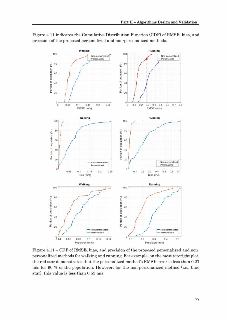
Part II – Algorithms Design and Validation
77
Figure 4.11 indicates the Cumulative Distribution Function (CDF) of RMSE, bias, and
precision of the proposed personalized and non-personalized methods.
Figure 4.11 – CDF of RMSE, bias, and precision of the proposed personalized and non-
personalized methods for walking and running. For example, on the most top-right plot,
the red star demonstrates that the personalized method’s RMSE error is less than 0.27
m/s for 90 % of the population. However, for the non-personalized method (i.e., blue
star), this value is less than 0.53 m/s.

Chapter 4 – Real-world gait speed estimation using a wrist sensor: A personalized approach
78
Eventually, Figure 4.12 displays the correlation between the actual and estimated
speed values through the proposed personalized and non-personalized methods.
Figure 4.12 – Estimated speed versus reference for the proposed personalized and non-
personalized methods.
4.5 Discussion
This study devised a personalized approach for accurate speed estimation during
walking and running using a wrist-mounted accelerometer and barometer under
various real-world conditions. Several terrain conditions, as well as speed ranges, were
considered for testing the method.
Our analysis showed that the correlation between features and step length might be
high when each individual was considered separately. However, it significantly dropped
by mixing the data of two or more individuals (see Figure 4.9). Consequently, to provide
a more accurate speed estimation, a personalized model was designed for each
individual. The personalized model was updated whenever new GNSS data were
acquired to adapt the model to the user’s new gait styles. As depicted in Figure 4.10, at
the beginning of the personalization procedure, the estimated speed error was relatively
high since there was not enough data to build a reliable speed model. However, as more
and more personalization data were given to the online RLS-based learning process,
the RMSE was gradually decreasing. The personalized approach relied on the same
features and similar rules as the non-personalized approach (RLS instead of the
conventional least square), where only the training data were different. The
personalized model was initialized through training by a small initial dataset coming
from the participant. An alternative was to train the initial model by the data belonging
to the whole population. However, the initial model that we proposed led to faster
convergence of the model and did not require a large training dataset involving high
numbers of participants.

Part II – Algorithms Design and Validation
79
The proposed personalized method was able to follow GNSS speed every second under
different speed ranges ([0.5 5.2] m/s) and environmental conditions (i.e., uphill, flat,
downhill). Compared to GNSS speed, the proposed method has achieved a proper RMSE
of 0.05 [0.04 0.06] m/s and 0.14 [0.11 0.17] m/s for walking and running, respectively.
It also provided almost zero bias for both walking and running. Eventually, the method
has obtained a very good precision of 0.06 [0.05 0.07] m/s and 0.18 [0.14 0.23] m/s for
walking and running, respectively (see Table 4.1). These errors determined how much
the proposed method was different from GNSS speed, which itself showed a median
measurement error of 0.12 m/s, despite the accuracy provided in the GNSS receiver
datasheet (0.05 m/s). Our algorithm performed better for walking than running, and
this was due to the greater robustness of the walking features extracted from hand
movement. Moreover, the proposed method was also robust enough to have similar
performance on both wrists.
In order to show the power of personalization, we compared the personalized method
with its non-personalized version where features, the model, and test data were the
same, and the difference came from the training approach. We demonstrated that using
50 times less training samples than the non-personalized method (i.e., 600-1200
samples compared to 30000-70000), the personalized method has achieved a better
RMSE, bias, and precision. It should also be noted that the personalized method was
trained by data of only one subject, compared to the non-personalized method trained
by data of 29 subjects. In particular, by personalization, the IQR of bias dropped by at
least ten times, which led to a more accurate estimation of average speed within a speed
measurement period. Moreover, the personalization led to a significant improvement of
the RMSE and precision (at least three times), which resulted in precise instantaneous
speed estimation. Figure 4.11 supports these results by showing that the proposed
personalized method performs excellent for almost all types of people where the range
of error is very low (e.g., RMSE varies in ranges [0.06 0.36] and [0.03 0.15] m/s for
walking and running, respectively).
On the other hand, the performance of the non-personalized method highly varies
among different types of people (e.g., RMSE varies in ranges [0.14 0.75] and [0.04 0.26]
for walking and running, respectively). Consequently, the personalized model is more
reliable than the non-personalized method. However, imagine a case where the data of
a specific person is not enough to train a reliable personalized model, depending on the
variety of his/her gait styles. In that case, the non-personalized method might perform
better due to the support of a much higher training data. This issue could be seen in
the most bottom left subfigure of Figure 4.11, where for a small number of subjects, the
precision of the non-personalized walking speed method was slightly better than the
personalized one. Figure 4.12 illustrated that personalization increased the correlation
between the reference and predicted speed by 23 % and 15 % for walking and running.
The results show that the personalized method’s performance was more similar to that
of the reference GNSS system than the non-personalized one.

Chapter 4 – Real-world gait speed estimation using a wrist sensor: A personalized approach
80
The personalized method used a few GNSS samples, which implies having the GNSS
activated only for a few minutes (i.e., 10 minutes) for each subject. This parsimonious
GNSS usage could be distributed over one or two weeks (e.g., some GNSS samples per
day) to obtain enough diversity in the gait styles (e.g., different speeds, terrain
conditions) of a user. In this study, we employed a random selection strategy to choose
a subset of GNSS samples to personalize the speed estimation model. However, a more
smart strategy could be designed (as a prospective of this study) to activate the GNSS
when there is new information in the user’s gait style. This procedure leads to capturing
the most informative GNSS samples by using the GNSS as less as possible.
In addition to personalization, we defined wrist-based biomechanically-derived features
to obtain a more accurate speed estimation. These features showed different degrees of
correlation with step length depending on the individual’s gait style, as was illustrated
for cadence in Figure 4.9. The results determined that each feature reached a 𝑅2 ≥ 0.41
for at least one subject. These results demonstrated that all the proposed features
conveyed useful information and had complementary effects. By selecting only a few
but relevant gait features, we reduced computation and complexity costs of the step
length model, which is essential for real-time algorithms implemented on portable
devices like wristwatches.
The results highlighted the dependence of the gait speed error on the speed values.
Overestimation for low speed and underestimation for high speed were observed
(Figure 4.8). One possible reason could be the linear model limitation, which was
preferred to decrease computation and algorithm complexity. Another reason might be
the limited number of training samples at low and high speed. Another issue is the
outliers, which could be seen in Figure 4.7. One possible reason for these might be the
lack of perfect synchronization between the proposed wrist-based speed estimation
method and the reference GNSS system. The wrist-based method used a 7-second
sliding window that prevented it from responding to rapid speed changes, which might
be quite probable in real-life situations. Hence, sometimes, there was a time delay
between the proposed personalized wrist-based method and the GNSS reference
system, which led to generating the outliers observed in our error plots. Apart from
this, the GNSS sometimes yielded very noisy data due to the low quality of satellite
signals or unexpected body movement, which alone could generate outliers. The
method, presented in section 4.3.2 and Figure 4.3, aimed at reducing noise in GNSS
data. However, other techniques for better GNNS signal enhancement could be
considered.
Compared to previous studies, the proposed personalized speed estimation algorithm
has achieved excellent performance even though the IMU placement on the wrist was
challenging, and measurements were performed in the free-living environment. For
walking, the personalized method provides a median error of 0.00 m/s and an IQR of
0.06 m/s. A recent non-personalized algorithm reached a median and IQR error of 0.02
and 0.18 m/s by an accelerometer and barometer (Fasel et al., 2017a). Methods based

Part II – Algorithms Design and Validation
81
on the feet IMU have also reported a mean error of 0.01 m/s and the precision of 0.08
m/s for indoor walking (Mariani et al., 2010), where both accelerometer and gyroscope
sensors were employed. Moreover, the shanks and thighs IMU-based algorithms used
at least three sensors to provide a precision of 0.10 m/s (Aminian et al., 2002). For
running, a few works have been introduced to estimate speed using IMU. The proposed
personalized method has obtained a median error of 0.00 m/s and an IQR of 0.18 m/s
for running speed estimation. The Feet-worn IMU was used to estimate running speed
with a median error of 0.07 m/s and a range of 0.13 m/s (de Ruiter et al., 2016). Yang et
al. also estimated running speed on a treadmill using an accelerometer and gyroscope
mounted on the shanks with an RMSE of 0.10 m/s (Yang et al., 2011). Moreover,
(Zrenner et al., 2018) tested four different speed estimation algorithms using an IMU
implemented into a shoe insole and reported a mean (± STD) error of 0.03 (±0.27) m/s.
The proposed method offers a versatile measurement tool that could be used in a variety
of target populations. In sports applications, it could help trainers and trainees optimize
their walking/running performances. In clinical applications, the method provides the
potential to monitor patients or older adults. For instance, in chapter 6 of this thesis,
we have applied this method to a large population to study the effect of various diseases
(e.g., obesity, frailty, cardiovascular disorders) or aging on people’s activity profile (i.e.,
gait speed). However, the proposed method would need to be complemented by other
GB detection techniques (as proposed in chapter 3 of this thesis) to automatically
classify GB that could then be used for speed estimation. Our analysis showed that
using only one unique model for walking and running speed estimation could increase
the error up to 4 times. Therefore, it is required to develop an algorithm to distinguish
between running and walking. Moreover, since the proposed personalized method has
been optimized for a healthy population, it might need some tuning and further
validation for patient populations.
To conclude, the present study provided a personalized approach for accurate, precise,
and low-power estimation of instantaneous speed during daily-life gait. It demonstrated
that personalization leads to a significant improvement of speed estimation based on
the wrist sensor (despite the challenges posed by the IMU location) by achieving results
comparable to the GNSS reference. As future work, the proposed algorithm could be
improved to manage non-linearity between the chosen features and the step length. It
could also be validated on abnormal gaits and integrated with an automatic GB
detection algorithm (Mannini et al., 2013; Zhang et al., 2012). Finally, a smart strategy
could be developed to minimize GNSS usage, thus reducing the system’s power
consumption.
4.6 Acknowledgment
The CTI Grant No. 18730.2 PFNM-NM supported the present study. We would like to
thank all participants who took part in our measurements.

Chapter 4 – Real-world gait speed estimation using a wrist sensor: A personalized approach
82
4.7 Appendix: Running speed estimation using foot-worn
inertial sensors2
This appendix shows how the proposed personalization idea could be applied to speed
algorithms on other sensor locations (i.e., feet-mounted IMU). In this study, three
approaches, based on direct integration, linear regression, and personalized model, are
designed. The main contribution to this study was in devising the personalized model
(explained in section 4.7.3.5), data collection and cleaning (section 4.7.3.1), and GNSS
data cleaning (4.7.3.2). A contribution was also made in the statistical analysis,
interpreting the results, and drafting the manuscript.
4.7.1 Abstract
The gait speed is the main outcome in running analysis. Contrary to treadmill running,
where the speed is fixed, most of the gait parameters are affected when running
overground at various speeds. Today, most wearable systems for running speed
estimation are based on GNSS. However, these devices have a high power consumption
and could suffer from sparse communication with the satellites. In this study, we
proposed three different approaches to estimate the overground speed in the running
based on the measurements of feet-worn IMU and compare them to GNSS considered
as reference. First, a method is proposed by direct strap-down integration of the foot
acceleration. Second, a feature-based linear model and finally, a personalized online-
model based on the RLS method were devised. We also evaluated the performance
differences between two sets of features; one automatically selected set (i.e., optimized)
and a set of features based on the existing literature. The data set of this study was
recorded in a real-world setting, with 33 healthy individuals running at low, preferred,
and high speed. The direct estimation of the running speed achieved an inter-subject
mean ± STD accuracy of 0.08 ± 0.1 m/s and a precision of 0.16 ± 0.04 m/s. In comparison,
the best feature-based linear model achieved 0.00 ± 0.11 m/s accuracy and 0.11 ± 0.05
m/s precision, while the personalized model obtained a 0.00 ± 0.01 m/s accuracy and
0.09 ± 0.06 m/s precision. The results of this study suggest that (1) the direct estimation
of the velocity of the foot are biased, and the error is affected by the overground velocity
and the slope; (2) the main limitation of a general linear model is the relatively high
inter-subject variance of the bias, which reflects the intrinsic differences in gait
patterns among individuals.; (3) this inter-subject variance could be nulled using a
personalized model.
Keywords: IMU, speed, running, linear prediction, personalization
2 This chapter is submitted as Falbriard, M., Soltani, A., & Aminian, K. (2020). Running speed estimation
using shoe-worn inertial sensors: direct integration, linear and personalized model to Frontiers in Sports
and Active Living. Contributions are as follows: design and implementation of the personalized model;
data collection; contribution to data analysis, performance evaluation and drafting the manuscript.

Part II – Algorithms Design and Validation
83
4.7.2 Introduction
The overground speed is the most useful metric in training and performance analysis
of running. Researchers have tried for decades to understand the physiological and
biomechanical adjustments occurring at different ranges of running speeds (Moore,
2016; Nummela et al., 2007; Thompson, 2017; Williams and Cavanagh, 1987). However,
most of the existing studies were performed in a controlled environment (i.e., treadmill
running inside a laboratory) where the runner has to adapt his gait to run at a constant
speed. In overground running, change of environment, surface, slope, obstacles, and
turns alter the gait and the running speed. Many studies have discussed the
biomechanical adaptations associated with running on a treadmill versus running
overground (Van Hooren et al., 2019). While standard motion capture (i.e.,
stereophotogrammetry and force plate) offers accurate measurements in laboratories,
the recent emergence of wearable systems is paving the shift towards studies carried
overground and in real-world conditions (Benson et al., 2018).
The real-world estimation of the overground speed is generally obtained using a body-
worn GNSS. Although these systems provide accurate and reliable measurement of the
locomotion speed (Terrier et al., 2000; Witte and Wilson, 2004), they suffer from several
limitations: (1) their high power consumption restricts their duration of use in portable
devices, (2) the communication between the receiver and the satellite is not always
guaranteed (e.g., indoor, near high buildings), and (3) the measurement accuracy
decrease during rapid changes of speed and position (Rawstorn et al., 2014; Varley et
al., 2012). As a solution to the latter limitation, systems based on the data fusion of
body-worn inertial and GNSS sensors have been proposed to monitor sports activities
(Brodie et al., 2008; Waegli and Skaloud, 2009; Zihajehzadeh et al., 2015). However, to
address the issue of power consumption and communication losses, IMU-based systems
must be able to estimate the speed without or with very limited input from a GNSS
device.
Several methods have been proposed to estimate the walking speed using IMU attached
to different body-segments (Aminian et al., 2002; Hu et al., 2013; Miyazaki, 1997;
Sabatini et al., 2005; Salarian et al., 2013; Zijlstra and Hof, 2003). One solution would
be to extend and adapt these methods to running. However, these methods often relied
on walking models or on estimating step length, which could not be directly applied to
running because of the aerial phases, where accelerometers are erroneous. Other
studies have used ML techniques to estimate the walking speed but did not validate
the results for running (Fasel et al., 2017c; Zihajehzadeh and Park, 2016).
To the authors’ knowledge, few studies proposed an accurate ambulatory method, based
on body-worn IMU, to estimate the overground speed of running, and even less did so
for instantaneous speed estimation. Two studies used a similar method (integration of
the acceleration signal) to calculate the velocity of the shank (Yang et al., 2011) and
foot (Chew et al., 2017) segments. However, the system’s error was computed over

Chapter 4 – Real-world gait speed estimation using a wrist sensor: A personalized approach
84
multiple strides, in a small range of speeds, and for level treadmill running. As
mentioned previously, the velocity estimated from the integration of segment
acceleration has limitations, mainly when the flight phase varies in a wide range or
when various slopes are experienced, as it is the case in the overground running.
Another study (Hausswirth et al., 2009) compared in-lab a commercialized speed
estimation device with a treadmill’s speed and reported a relatively low accuracy
considering that the system required a subject-specific calibration. Subject-specific NN
was also devised to assess the running speed in free-living conditions using only triaxial
accelerometric measurements. However, the model needed a calibration/learning phase
for each runner and was validated for the mean speed using a few trials (HERREN et
al., 1999). However, one study exploited the personalized calibration and proposed a
model based solely on the contact time (De Ruiter et al., 2016). Although the authors
obtained a low RMSE (<3%), these results were not instantaneous estimations but
rather the average speed over bouts of 125 meters. Besides, a more recent study (Soltani
et al., 2019) based on wrist-worn IMU suggested that better results could be achieved
by including more features to the model.
The objective of the current study was three-fold. First, we aimed to extend an existing
walking algorithm based on strap-down integration of foot acceleration and show its
limitation for running speed estimation. Then we proposed a new linear model to
predict the running speed at each step and in real-world condition, based on relevant
features extracted from feet acceleration and angular velocity. Finally, we investigated
how personalization improved the system’s performances using additional data, such
as occasional GNSS inputs. We compared each method to the GNSS speed, considered
as the ground truth, obtained during outdoor measurements of overground running, at
different speeds and slopes.
4.7.3 Methods
4.7.3.1 Protocol and instrumentation
33 healthy and active participants, 18 males (age: 38 ± 9 y.o.; size: 180 ± 7 cm; weight:
76 ± 9 kg), 15 females (age: 36 ± 10 y.o.; size: 165 ± 7 cm; weight: 59 ± 7 kg), without
any symptomatic musculoskeletal injuries participated to this study. The
measurements were performed in real-world conditions with sections of uphill,
downhill, and level running. We asked the participants to run the same circuit three
times, once at self-adjusted normal, fast, and slow speeds (Figure 4.13, left). The periods
of rest and the walking bouts, in between the running segments, were manually
removed from the analysis. The local ethics committee approved the present protocol,
and we conducted the measurements in agreement with the declaration of Helsinki.

Part II – Algorithms Design and Validation
85
Figure 4.13 – (Left) The elevation and speed of the running circuit. This figure was
adapted from (Soltani et al., 2019). (Right) the definition of the foot functional frame
(FF) and global frame (GF) used in this study.
Each participant was equipped with two time-synchronized IMU (Physilog 4, Gait Up,
Switzerland) strapped on the shoe’s dorsum. Each sensor included a triaxial
accelerometer, a triaxial gyroscope, and a barometer. The barometer was sampled at 50
Hz. Acceleration (± 16 g) and angular velocity (± 2000 deg/s) were recorded at 500 Hz
and were calibrated according to (Ferraris et al., 1995) before each measurement
session. Furthermore, a GNSS receiver (CAMM8Q, u-blox, CH) with an external active
antenna (ANN-MS, u-blox, CH) was mounted on the head using Velcro attached to a
cap. GNSS was used as a reference system for the estimation of the running speed. The
GNSS receiver was set to pedestrian mode with a sampling frequency of 10 Hz. With
such a configuration, the manufacturer’s datasheet reported a median error of 0.05 m/s
for instantaneous speed estimation. MATLAB software (R2018b, MathWorks, Natick,
MA USA) was used for all the data processing steps without the need for publicly
available libraries.
4.7.3.2 Estimation of reference GNSS speed
The reference speed obtained from the GNSS receiver was processed according to
(Soltani et al., 2019) and in two steps (Figure 4.14). First, we enhanced the signal by
removing the outliers that did not correspond to running; hence, we removed all
recorded speed samples outside the 5-20 km/h range. Moreover, the GNSS receiver
provided an estimation of the accuracy of each observation; hence we discarded any
data-point with an error higher than 0.15 m/s. This process retrieved an unevenly
sampled reference speed signal. We applied a moving average of 0.5-second width (in
10 Hz), followed by linear interpolation to obtain an equally-spaced time series at 10
Hz. In the second step, the signal was down-sampled to provide the reference speed
(𝑣𝑟𝑒𝑓), after a fourth-order low-pass Butterworth filter with the cut-off frequency at 0.25
Hz to reduce the noise.

Chapter 4 – Real-world gait speed estimation using a wrist sensor: A personalized approach
86
Figure 4.14 – Pre-processing steps applied to the GNNS measurements of speed to
obtain the reference speed estimation. This figure was adapted from (Soltani et al.,
2019)
4.7.3.3 Speed estimation based on direct integration of foot acceleration
This section describes the sequence of transformations applied to the IMU and
barometer data to extract the gait features. The whole process could be summarized in
four tasks: pre-processing, temporal analysis, spatial analysis, and foot speed
estimation (Figure 4.15).
Figure 4.15 – Steps performed on the IMU acceleration 𝑎( ), angular velocity 𝜔( ), and
barometric pressure ( ) measurements. The outputs were later used for feature
extraction; the slope 𝑠( ), the speed of the foot 𝑣𝑓𝑜𝑜𝑡( ), the pitch angle ( ), contact time
𝐶𝑇, flight time 𝐹𝐿𝑇, swing phase duration 𝑆𝑊𝑇, step duration 𝑆𝑇𝑃 and stride duration
𝑆𝑇𝑅.
4.7.3.3.1 Pre-processing
First, a fourth-order low-pass Butterworth filter (𝐹𝑐 = 50 Hz) was applied on the raw
acceleration, 𝑎( ), and angular velocity, 𝜔( ), signals to reduce the noise. Then the IMU

Part II – Algorithms Design and Validation
87
signals were aligned with the foot segment by computing the rotation matrix that
transforms the data recorded in the technical frame of the sensors into the functional
frame (FF) of the foot (Figure 4.13, right). For this purpose, we used the measurements
of level normal walking (Figure 4.13, left) and a previously reported calibration method
(Falbriard et al., 2018). This process aligned the -axis of the IMU with the vertical axis
of the foot, pointing upward, the -axis to the mediolateral axis, pointing to the right
side of the subject, and the 𝑥-axis to the longitudinal axis, pointing towards the forefoot.
Throughout this study, if not mentioned otherwise, the data are reported in the
functional frame of the foot.
The last phase in pre-processing was estimating the overground slope. As the running
mechanics differ between level, uphill, and downhill running (Vernillo et al., 2017), we
assumed that the elevation difference between successive steps would be a relevant
input for the model. Therefore, the barometric pressure was converted by the
hypsometric equation to the altitude signal (Bolanakis, 2017), smoothed by applying a
4-seconds moving average filter, and down-sampled to 1 Hz time-series. The slope, 𝑠( ),
was defined as the altitude difference between two samples spaced by 5 seconds,
byassuming that altitude changes shorter than 5 seconds would not significantly affect
the running speed.
4.7.3.3.2 Temporal analysis
Temporal events detection was performed as described in (Falbriard et al., 2018) by
segmenting the race into midswing-to-midswing cycles and detecting of several
temporal events within each cycle. Midswing was detected as the positive peaks
observed on the pitch axis (FF -axis) of the angular velocity measurements. Moreover,
we improved the robustness of the peak detection algorithm by applying the YIN auto-
correlation method (De Cheveigné and Kawahara, 2002) over a 10-second sliding
window (5-seconds overlap) to obtain an approximation of the cadence and set an
adequate minimum time difference between the two peaks. The 𝐼𝐶, defined as the
moment when the foot initiates contact with the ground at landing, and terminal
contact (𝑇𝐶), defined as the instant when the toes leave the ground during the pushing
phase, were then detected within each cycle using the two minimums of the pitch
angular velocity. Moreover, we defined the event MinRot as the time-point where the
norm of the angular velocity (||𝜔( )||) is minimum within the stance phase (i.e., between
𝐼𝐶 and 𝑇𝐶).
4.7.3.3.3 Spatial analysis and foot speed estimation
This process aimed to measure the foot’s orientation in the global frame (GF), remove
the Earth’s gravitational acceleration from the recorded acceleration, and integrate the
corrected acceleration to obtain the speed of the foot. In GF, the 𝑥-axis was in the
running direction, the -axis corresponds to the axis perpendicular to the ground
surface, and the -axis was defined by the cross-product of the and 𝑥-axes (Figure
4.13). Using a previously validated technique (Falbriard et al., 2020), foot orientation

Chapter 4 – Real-world gait speed estimation using a wrist sensor: A personalized approach
88
was obtained in GF, and foot acceleration in FF was expressed in GF, and the
gravitational acceleration (𝑔 = [0 0 9.81] m/s2 ) removed. The resulting acceleration (in
GF) was integrated using a trapezoidal rule to get a first estimate of the speed of the
foot. We considered the speed of the foot to be zero during the stance phase and,
therefore, estimated and removed the integration drift by linearly resetting the speed
between MinRot and 𝑇𝐶 of each stance phase. Note that we preferred MinRot to the 𝐼𝐶
for drift resting since MinRot corresponds to the time sample when the foot is the closest
to a static state, reportedly used as the integration limits in walking gait analysis
(Mariani et al., 2010). We finally applied the inverse of the quaternions mentioned
above to get the drift-corrected speed of the foot segments (𝑣𝑓𝑜𝑜𝑡( )) in the FF.
4.7.3.4 Development of a linear model for speed prediction
4.7.3.4.1 Feature extraction, linearization, and outliers removal
First, we extracted several parameters, 𝑝𝑗, for each step, which was later used as inputs
for the speed estimation model. As several studies reported on the association between
the changes in the duration of the gait phases and the running speed (Högberg, 1952;
Nummela et al., 2007; Saito et al., 1974), we computed the ground contact time (𝐶𝑇),
the flight time (𝐹𝐿𝑇), the swing time (𝑆𝑊𝑇), the step duration (𝑆𝑇𝑃), and the stride
duration (𝑆𝑇𝑅) for each step 𝑖, where 𝑖 = 1, … , 𝑁, and 𝑁 is the total number of steps
(4.21)-(4.25).
𝐶𝑇𝑖 = 𝑇𝐶𝑖 − 𝐼𝐶𝑖 (4.21)
𝐹𝐿𝑇𝑖 = 𝐼𝐶𝑖+1 − 𝑇𝐶𝑖 (4.22)
𝑆𝑊𝑇𝑖 = 𝐼𝐶𝑖+2 − 𝑇𝐶𝑖 (4.23)
𝑆𝑇𝑃𝑖 = 𝐼𝐶𝑖+1 − 𝐼𝐶𝑖 (4.24)
𝑆𝑇𝑅𝑖 = 𝐼𝐶𝑖+2 − 𝐼𝐶𝑖 (4.25)
As a few strides suffered from misdetections, outliers were removed according to (1) a
valid stride must last between 0.37 and 2.5 seconds, and (2) the flight phase (𝐹𝐿𝑇) must
be greater than zero.
Pitch angle, , at the 𝐼𝐶 was extracted as the angle between the longitudinal axis of the
foot (FF 𝑥-axis) and the ground surface (𝑥 and -axis in GF). A positive pitch angle
corresponds to a rear-foot landing (i.e., talus region lower than the toes) and a negative
pitch angle to a forefoot strike.
We also extracted several statistics from the acceleration 𝑎( ), the angular velocity 𝜔( ),
the foot speed 𝑣𝑓𝑜𝑜𝑡( ), and the slope 𝑠( ) time-series. Moreover, since 𝑎( ), 𝜔( ), and
𝑣𝑓𝑜𝑜𝑡( ) were 3D signals, these statistics were computed for each axis (i.e., 𝑥, , and )
and the norm of the signal. Note that the features were captured on the signals of a

Part II – Algorithms Design and Validation
89
single stride (i.e., between 𝐼𝐶𝑖 and 𝐼𝐶𝑖+2, where 𝑖 = 1,… ,𝑁) before applying the
statistical functions. We opted for a stride-based segmentation instead of the step-based
segmentation because a stride corresponds to one period of gait and, therefore, is more
likely to capture the complete pattern of a cycle. Besides, the list of selected features
(Table 4.3) aimed to collect information on the intensity of the signal (e.g., mean, STD,
RMS), the shape of its distribution (e.g., skewness, kurtosis), and its shape in a
compressed format (e.g., coefficient of the auto-regressive model). Moreover, as the
temporal parameters, (4.21)-(4.25), already hold relevant periodic information, we did
not consider features in the frequency domain.
Table 4.3 – List of the features extracted for each stride on the continuous acceleration
𝑎( ), angular velocity 𝜔( ), speed 𝑣𝑓𝑜𝑜𝑡( ), and slope 𝑠( ). In the name of the feature,
variables < 𝑇 > and < 𝐶 > correspond to the label of the signal and the channel,
respectively. Hence < 𝑇 > must be replaced by 𝑎, 𝜔, 𝑣𝑓𝑜𝑜𝑡, or 𝑠 while < 𝐶 > must be
replaced by 𝑥, , , or norm.
Type Feature Description
Intensity 𝑚𝑒𝑎𝑛_ < 𝑇 > _ < 𝐶 > Mean value
𝑠 𝑑_ < 𝑇 > _ < 𝐶 > STD
𝑚𝑒𝑑_ < 𝑇 > _ < 𝐶 > Median
𝑖𝑞𝑟_ < 𝑇 > _ < 𝐶 > IQR
𝑚𝑎𝑥_ < 𝑇 > _ < 𝐶 > Maximum
𝑟𝑚𝑠_ < 𝑇 > _ < 𝐶 > Root-mean-square
Shape 𝑘𝑢𝑟 _ < 𝑇 > _ < 𝐶 > Kurtosis
𝑠𝑘𝑒 _ < 𝑇 > _ < 𝐶 > Skewness
Compression 𝑎𝑟𝑚1_ < 𝑇 > _ < 𝐶 > First coefficient of the auto-regressive model of order 3
𝑎𝑟𝑚2_ < 𝑇 > _ < 𝐶 > Second coefficient of the auto-regressive model of order 3
𝑎𝑟𝑚3_ < 𝑇 > _ < 𝐶 > Third coefficient of the auto-regressive model of order 3
Before proceeding to the selection of the best features, we visualized the relation
between the reference speed 𝑣𝑟𝑒𝑓( ) and the features individually. Based on our
observations, we identified three functions that improved the linear relationship
between the reference speed and some of the input features; 𝑓1(𝑝) = 𝑝2, 𝑓2(𝑝) = 𝑝3,
and 𝑓3(𝑝) = 1/𝑝. The functions 𝑓1, 𝑓2, and 𝑓3 were applied to all the features, and the
results were added to the list of features. Finally, we also included several
anthropometric parameters to the set of features, such as the size, weight, gender, and
age of the participants.
4.7.3.4.2 Data set configuration
We divided the data into three subsets: validation, training, and testing sets. The
participants were randomly distributed into the three subsets. It is important to note

Chapter 4 – Real-world gait speed estimation using a wrist sensor: A personalized approach
90
that all the steps of a single individual were attributed to only one of the subsets; this
removed the performance bias associated with the models trained and tested on
measurements originating from the same subjects (Halilaj et al., 2018). Figure 4.16
shows the data from each set with different colors and illustrates their functions.
We used the 10 subjects (30 %) from the validation set for feature selection (in orange
in Figure 4.16), and the 23 remaining participants (70 %) were used interchangeably
for training (in blue in Figure 4.16) and testing (in green in Figure 4.16) of the model
according to the leave-one-subject-out cross-validation method. We emphasize on the
fact that the validation set was not included in the evaluation of the model and served
exclusively for feature selection. We distinguished the development set from the other
sets to lessen the risks of overfitting and preferred a leave-one-subject-out approach to
assessing the model’s performance due to the relatively low number of individuals
present in this study. Moreover, such a method allowed us to identify potential outliers
in the participants and later find collections of subjects with similar biases.
The leave-one-subject-out cross-validation method functioned as followed: we trained
the model using the data from 22 subjects (training set) and tested on the data from
one individual (testing set). We then repeated this process, such that each participant
appeared once in the testing set.
Figure 4.16 – Schematic representation of the data repartition into the validation
(blue), training (orange), and testing (green) set. The validation set was used for feature
selection, the training set to train the coefficients of the linear model, and the testing
set to evaluate the performance of the predictions. The features are represented as 𝑝𝑗
and the linearization function as 𝑓1(𝑝𝑗), 𝑓2(𝑝𝑗) and 𝑓3(𝑝𝑗).
4.7.3.4.3 Automatic feature selection
Here, we selected the features (𝑃𝑎𝑢𝑡𝑜) to minimize the Mean Square Error (MSE) of the
speed estimation model using the ordinary least squares method. The leave-one-

Part II – Algorithms Design and Validation
91
subject-out method was applied with 11 subjects for training and one subject to evaluate
the error of the predictions (Figure 4.16). The automatic feature selection process
started with an empty set of inputs and sequentially added the parameters 𝑝𝑗 or their
transform (𝑓1, 𝑓2, 𝑓3), which minimized the average MSE among all the subjects. This
method is known as the forward stepwise selection process and has proven to be reliable
on large feature space (John et al., 1994; Kohavi and John, 1997). The algorithm
stopped including new parameters if the gain in the average MSE was lower than 1 %
of the previous MSE recorded. We deliberately set a low 1 % criterion to obtain a
possibly unnecessary large number of inputs knowing that the model is trained using
the LASSO method (Tibshirani, 1996) with shrinkage of the redundant features. To
ensure that the features contributed equally to the MSE estimation, we rescaled the
inputs using a robust -score normalization method (Jain et al., 2005); after
normalization, the feature’s mean was equal to zero, and the median absolute deviation
equal to one (less sensitive to outliers than the variance of one).
4.7.3.4.4 Comprehensive selected features
Although a supervised and automatic feature selection method might retrieve the
subset with the best prediction performance on a given set of parameters, the results
are sometimes difficult to interpret. Hence it is generally recommended also to evaluate
the performance of a comprehensive set of features selected based on their
biomechanical relevance (Halilaj et al., 2018). Based on the findings of previous
research in running, we defined a list of features (𝑃𝑚𝑎𝑛𝑢𝑎𝑙) known to be affected by
variations in the running speed. Similarly to the automatic selection of features, we
willingly selected many input features, potentially intercorrelated, knowing that
optional inputs will be discarded later in the training stage. In summary,
comprehensive features included the following:
Anthropometric features: the height because taller individuals are likely to have
longer step length, thus higher speed, than shorter individuals with similar flight
times.
Temporal features: the 𝐶𝑇, 𝐹𝐿𝑇, and 𝑆𝑇𝑅 contain relevant information about the
stride frequency and were shown to decrease with an increase in the running speed
(Chapman et al., 2012; Nummela et al., 2007; Saito et al., 1974).
Speed and spatial features: the average speed of the foot (𝑚𝑒𝑎𝑛_𝑣𝑓𝑜𝑜𝑡_𝑛𝑜𝑟𝑚)
obtained with a direct integration; the maximum angular velocity of the foot in the
sagittal plane (𝑚𝑎𝑥_𝜔_ ) assuming faster swing involves higher speed; the RMS
value of the angular velocity norm (𝑟𝑚𝑠_𝜔_𝑛𝑜𝑟𝑚) since higher speed should result
in higher dynamic movements; the maximum of the acceleration norm
(𝑚𝑎𝑥_𝑎_𝑛𝑜𝑟𝑚) as it was demonstrated in previous studies that tibial peak
accelerations increased with faster-running velocities (Sheerin et al., 2019); and the
average slope (𝑚𝑒𝑎𝑛_𝑠) since uphill and downhill might affect the running speed.

Chapter 4 – Real-world gait speed estimation using a wrist sensor: A personalized approach
92
4.7.3.4.5 Training and testing of the model
The linear model was trained and tested with the leave-one-subject-out cross-validation
method. For each individual, the performance of the speed prediction was evaluated
with the model’s coefficients trained on 22 other subjects. This approach was preferred
to a traditional split of the data into two datasets (e.g., 70 % training and 30 % testing
repartition) due to the restricted number of subjects available after the feature selection
phase. Besides, the leave-one-subject-out procedure allowed us to detect potential
outliers in the participants and, therefore, possibly identify the sources of poor
estimation results.
The least-squares regression coefficients were trained using the LASSO method
(Tibshirani, 1996), with scaled inputs to have zero mean and a variance of one, and
equally distributed the observations’ weights at the initialization stage. To limit
overfitting risks, we selected the model with the smallest number of inputs, if any new
input would improve the MSE by less than 2 %.
Since we observed some disparity in the dataset (the steps between 2.5-4 m/s were over-
represented), we used a random under-sampling (RUS) method to deal with the issue
of class imbalance (Pes, 2020). This process started by dividing the range of reference
speeds into five equally spaced groups, from 1.4 to 2.2 m/s, 2.2 to 3 m/s, 3 to 3.8 m/s, 3.8
to 4.6 m/s, and 4.6 to 5.4 m/s. We randomly selected the same number of steps from
each group based on the group with the least number of steps (i.e., down-sampling of
the majority). We repeated this process ten times, generating ten versions of the under-
sampled data set and used these subsets independently. In other words, we trained and
tested the model ten times for each individual.
Finally, we investigated the changes in the speed prediction when input features were
averaged over consecutive steps. Instead of using a single step granularity for running
speed, averaging over several steps might conceivably improve the precision (i.e.,
random error) of the model. We tested this approach on an even number of steps (i.e.,
2, 4, 6, 8, and 10), for it equally includes the sensor’s information from both feet. In
order to avoid grouping non-consecutive steps, we applied this averaging process before
under-sampling the inputs.
4.7.3.5 Personalized model
4.7.3.5.1 Running speed estimation algorithm
Recently, online personalization methods have emerged in the field of human
movement analysis. For instance, such an approach demonstrated significant
improvement in speed estimation performances (Soltani et al., 2019). The objective is
to personalize a generic speed estimation model based on the sporadic reference data
obtained from a GNSS device. We describe the online-learning procedure used in this
study in the following; we define n as the observation (or sample) index used for the

Part II – Algorithms Design and Validation
93
personalization where each sample corresponds to one stride. Therefore, if we have 𝑀
samples (i.e., strides) for the personalization, then 𝑛 ∈ {1, 2, 3, … ,𝑀}.
Let’s 𝑄 be the number of features in each stride. We defined 𝒑 as the feature vector
and 𝑠𝑙𝑛 as the reference stride length for the 𝑛-th stride according to (4.26) and (4.27).
Here, 𝑝𝑗[𝑛] is a symbolic name for the 𝑗-th feature of the 𝑛-th stride. Moreover, 𝑣𝑟𝑒𝑓[𝑛]
is the GNSS speed of the 𝑛-th stride.
𝒑 = [1 𝑝1[𝑛] 𝑝2[𝑛] … 𝑝𝑄[𝑛]] (4.26)
𝑠𝑙𝑛 = 𝑣𝑟𝑒𝑓[𝑛] ×1
𝑆𝑇𝑅𝑛
(4.27)
For 𝒑 we used the selected features in 𝑃𝑚𝑎𝑛𝑢𝑎𝑙or 𝑃𝑎𝑢𝑡𝑜 based on results obtained in the
linear model. We first modeled the stride length through RLS and then multiplied that
by the stride frequency to obtain the running speed. The RLS is a real-time and
computationally effective online learning method, which does not need to have or store
all the training data from the beginning of training.
Let 𝑃𝑛 and 𝑆𝐿𝑛 be the feature matrix and the vector of actual stride length defined in
(4.28) and (4.29), respectively.
𝑃𝑛 = [
𝒑𝟏⋮𝒑 ]
(4.28)
𝑆𝐿𝑛 = [𝑠𝑙1⋮𝑠𝑙𝑛
]
(4.29)
Using the RLS approach, 𝑆𝐿𝑛 could be modeled as in (4.30), where 𝛽𝑛 is the coefficient
of the model trained using 𝑛 observations. If 𝑃𝑛−1 and 𝛽𝑛−1 are the feature matrix and
model coefficients estimated using 𝑛 − 1 samples, then once we obtain a new sample
(𝒑 and 𝑠𝑙𝑛) for the personalization, 𝛽𝑛 could be recursively estimated through (4.30).
𝛽𝑛 = 𝛽𝑛−1 + 𝐷𝑛𝒑 (𝑠𝑙𝑛 − 𝒑 𝑻𝛽𝑛−1) (4.30)
Where 𝐷𝑛, known as the dispersion matrix, itself, is recursively estimated by having
only 𝐷𝑛−1 (i.e., the dispersion matrix estimated using 𝑛 − 1 samples) and the new
personalization data (i.e. 𝒑 and 𝑠𝑙𝑛) according to (4.31). Here, 𝐾𝑛 is defined as (4.32).
𝐷𝑛 = 𝐷𝑛−1(𝐼 − 𝒑 (𝐼 + 𝐾𝑛)−1𝒑
𝑻𝐷𝑛−1) (4.31)
𝐾𝑛 = 𝒑 𝑻𝐷𝑛−1𝒑 (4.32)
For each individual, ten strides from the training set were used to initialize the RLS
recursion process.

Chapter 4 – Real-world gait speed estimation using a wrist sensor: A personalized approach
94
4.7.3.5.2 Cross-validation
The data set was organized differently for the personalization process to consider each
individual’s gait style and minimize the training data from GNSS. Data from each
individual was divided into bouts of 10 strides, and half of these bouts were assigned
randomly to the training set and the other half to the testing set of that same individual.
Consequently, we trained and evaluated the models for each individual separately,
using the uniquely the data from that same individual.
4.7.3.6 Statistical analysis
We evaluated the performance of the model by computing the error on the training and
testing sets. We did so going from a single step to a ten-steps resolution according to
the configuration of the inputs. For each of the RUS iteration, the intra-subject accuracy
(or bias) and precision were estimated using the mean and STD, respectively. The
normality of the speed error was tested using the Lilliefors test, and in the case of non-
normal distribution, the mean was replaced by the median and STD by the IQR. To
better understand the performance of the system, the intra-subject RMS error was
calculated, and the Pearson correlation coefficient was used to assess the linear
dependence of the predictions. Since we used the leave-one-subject-out method for
training and testing, the results were reported by computing the mean, the STD, the
minimum and the maximum on the intra-subject biases, precision, RMS error, and
correlation coefficients. Agreement between the reference GNSS speed and the
estimated speed was illustrated with Bland-Altman plots (Bland and Altman, 2003).
Furthermore, to evaluate the distribution of the errors and possible overfitting, we used
the CDF of step absolute error for both training and testing sets.
4.7.4 Results
4.7.4.1 Direct speed estimation
Two subjects were excluded from the data set; because of the poor quality of the GNSS
measurements or because of an improper fixation of the IMU on the shoe and high
Signal to Noise Ratio of the kinematic data. Since it required no learning, the direct
speed estimation method was performed on the 63435 steps available in this study. We
observed an inter-subject mean ± STD (min, max) of 0.08 ± 0.10 (-0.12, 0.27) m/s for the
bias, 0.16 ± 0.04 (0.08, 0.25) m/s for the precision, 0.20 ± 0.06 (0.08, 0.34) for the RMSE.
The relation between the speed estimation error and the overground velocity is
presented in Figure 4.17, and the effect of the slope in Figure 4.18.

Part II – Algorithms Design and Validation
95
Figure 4.17 – Bland-Altman plot of the agreement between the direct speed estimation
method (𝑣𝑓𝑜𝑜𝑡) and the GNSS reference (𝑣𝑟𝑒𝑓). The error was estimated with a
granularity of one step.
Figure 4.18 – The step by step error of the direct speed estimation method (𝑣𝑓𝑜𝑜𝑡) in
relation to the slope of the ground surface.
4.7.4.2 Automatic feature selection
In total, we used the 20084 strides of the validation set to select 28 features out of the
668 features available. The feature selection process stopped at an average MSE of
0.0057 m/s (Figure 4.19), which corresponded to a 1.12 % improvement compared to the

Chapter 4 – Real-world gait speed estimation using a wrist sensor: A personalized approach
96
previous step with 27 features. The selection process was repeated 100 times (i.e., 10
times for each of the 10 subjects) and led to the set of features presented in Table 4.4.
Figure 4.19 – MSE of the speed estimation during the forward stepwise selection
process. In grey, the MSE of each subject, and blue the inter-subject average.
Table 4.4 – The ordered list of the features automatically selected by the forward
stepwise selection algorithm.
# Label 𝑓(𝑝) # Label 𝑓(𝑝)
1 mean_a_norm - 15 mean_𝑣𝑓𝑜𝑜𝑡_y p2
2 mean_𝑣𝑓𝑜𝑜𝑡_norm - 16 median_ω_norm p-1
3 iqr_a_norm - 17 median_ω_x -
4 - 18 skew_𝑣𝑓𝑜𝑜𝑡_norm -
5 mean_s p2 19 iqr_𝑣𝑓𝑜𝑜𝑡_norm p-1
6 STR p-1 20 max_𝑣𝑓𝑜𝑜𝑡_y p-1
7 median_a_x p3 21 mean_ω_y -
8 median_ω_z p3 22 rms_a_x p3
9 max_𝑣𝑓𝑜𝑜𝑡_norm - 23 median_𝑣𝑓𝑜𝑜𝑡_x -
10 median_a_y p3 24 std_a_norm p-1
11 mean_𝑣𝑓𝑜𝑜𝑡_x p2 25 skew_ω_norm -
12 skew_𝑣𝑓𝑜𝑜𝑡_y p-1 26 skew_ω_z p2
13 median_𝑣𝑓𝑜𝑜𝑡_y - 27 std_a_x p-1
14 std_ω_z - 28 arm3_𝑣𝑓𝑜𝑜𝑡_y p-1

Part II – Algorithms Design and Validation
97
Out of the 28 features selected, 16 (57 %) resulted from one of the three linearization
functions (𝑓1, 𝑓2, 𝑓3), one feature from the temporal analysis (𝑆𝑇𝑅), one from the
orientation estimation (). The other features are statistics extracted from the different
time series (i.e., acceleration 𝑎( ), angular velocity 𝜔( ), the velocity of the foot segment
𝑣𝑓𝑜𝑜𝑡( ), and the slope 𝑠( )).
4.7.4.3 Linear model
In total, 43351 steps were used to train and test the linear model. Due to the subdivision
of the data associated with the leave-one-subject-out method, we used, for each
individual, a mean ± STD (min, max) of 41287 ± 188 (41032, 41642) steps for training
and 2064 ± 188 (1709, 2319) steps for testing.
When the 𝑃𝑎𝑢𝑡𝑜 feature set was used for training, the LASSO method always favored
the same 7 inputs (𝑃𝑎𝑢𝑡𝑜,𝑏𝑒𝑠𝑡) among the 28 features previously selected (Table 4.4):
𝑃𝑎𝑢𝑡𝑜,𝑏𝑒𝑠𝑡 [𝑚𝑒𝑎𝑛_𝑎_𝑛𝑜𝑟𝑚, 𝑓1(𝑚𝑒𝑎𝑛_𝑠), 𝑓3(𝑆𝑇𝑅), 𝑓2(𝑚𝑒𝑑𝑖𝑎𝑛_𝜔_ ),
𝑚𝑎𝑥 _𝑣𝑓𝑜𝑜𝑡_𝑛𝑜𝑟𝑚, 𝑓1(𝑚𝑒𝑎𝑛_𝑣𝑓𝑜𝑜𝑡_ ), 𝑓3(𝑚𝑒𝑑𝑖𝑎𝑛_𝜔_𝑛𝑜𝑟𝑚)]
In comparison, with 𝑃𝑚𝑎𝑛𝑢𝑎𝑙 the LASSO method selected 4 inputs (𝑃𝑚𝑎𝑛𝑢𝑎𝑙,𝑏𝑒𝑠𝑡):
𝑃𝑚𝑎𝑛𝑢𝑎𝑙,𝑏𝑒𝑠𝑡 = [𝑟𝑚𝑠_𝜔_𝑛𝑜𝑟𝑚,𝑚𝑒𝑎𝑛_𝑣𝑓𝑜𝑜𝑡_𝑛𝑜𝑟𝑚,𝑚𝑒𝑎𝑛_𝑠, 𝐶𝑇]
The linear predictor performances over the testing set are shown in Table 4.5; the inter-
subject mean, STD, minimum, and maximum are presented for the bias, the precision,
the RMSE, and the correlation coefficients. The running speed estimation results are
presented for single-step resolution and where the inputs were averaged over 2, 4, 6, 8,
and 10 steps before being used by the linear model.
In comparison, when we used a moving average (4 steps) on the output of the speed
estimation model (i.e., not the inputs as in Table 4.5), then we obtained an inter-subject
mean ± STD (min, max) bias of 0.00 ± 0.10 (-0.17, 0.17) m/s, precision of 0.13 ± 0.05
(0.06, 0.23) m/s, RMSE of 0.14 ± 0.05 (0.08, 0.28) m/s, and correlation coefficients of
0.985 ± 0.010 (0.956, 0.997). The agreement between the speed estimation using
𝑃𝑎𝑢𝑡𝑜,𝑏𝑒𝑠𝑡 (𝑣𝑒𝑠𝑡) and the reference GNSS system is presented for each stride (grey dots)
and each individual (blue circles) in Figure 4.20.

Chapter 4 – Real-world gait speed estimation using a wrist sensor: A personalized approach
98
Table 4.5 – Inter-subject mean, STD, minimum, and maximum of the system’s bias,
precision, RMSE, and the linear correlation coefficient (R). The results are presented
for each configuration of inputs (𝑃𝑎𝑢𝑡𝑜,𝑏𝑒𝑠𝑡 and 𝑃𝑚𝑎𝑛𝑢𝑎𝑙,𝑏𝑒𝑠𝑡). Here, “Feat.” means
features.
Feat. Step Bias, m/s Precision, m/s RMSE, m/s R
mean STD min max mean STD min max mean STD min max mean STD min max
𝑃𝑎𝑢𝑡𝑜,𝑏𝑒𝑠𝑡
1 0.00 0.10 -0.17 0.17 0.14 0.05 0.08 0.24 0.16 0.05 0.10 0.28 0.985 0.010 0.956 0.997
2 0.00 0.11 -0.17 0.18 0.13 0.05 0.06 0.23 0.14 0.05 0.08 0.27 0.989 0.009 0.957 0.998
4 0.00 0.11 -0.17 0.19 0.12 0.06 0.05 0.24 0.12 0.05 0.07 0.24 0.990 0.009 0.961 0.998
6 0.00 0.11 -0.17 0.18 0.11 0.05 0.05 0.23 0.12 0.04 0.06 0.21 0.990 0.009 0.952 0.999
8 0.00 0.11 -0.18 0.19 0.11 0.05 0.05 0.23 0.12 0.05 0.06 0.23 0.991 0.009 0.952 0.999
10 0.00 0.11 -0.17 0.19 0.11 0.05 0.05 0.23 0.11 0.04 0.06 0.23 0.992 0.008 0.965 0.999
𝑃𝑚𝑎𝑛𝑢𝑎𝑙,𝑏𝑒𝑠𝑡
1 0.00 0.11 -0.22 0.17 0.15 0.06 0.09 0.29 0.18 0.07 0.11 0.37 0.983 0.009 0.961 0.997
2 0.00 0.11 -0.23 0.18 0.13 0.06 0.07 0.26 0.15 0.06 0.09 0.29 0.988 0.008 0.963 0.997
4 0.00 0.11 -0.23 0.20 0.12 0.06 0.06 0.26 0.14 0.06 0.08 0.24 0.989 0.009 0.959 0.998
6 0.00 0.12 -0.23 0.19 0.12 0.06 0.06 0.24 0.13 0.06 0.06 0.24 0.990 0.009 0.956 0.999
8 0.00 0.12 -0.23 0.20 0.11 0.06 0.05 0.24 0.13 0.06 0.06 0.24 0.991 0.009 0.944 0.999
10 0.00 0.12 -0.24 0.20 0.11 0.06 0.05 0.24 0.12 0.06 0.06 0.24 0.991 0.008 0.964 0.999
Figure 4.20 – Bland-Altman plot of the speed estimation (𝑣𝑒𝑠𝑡) obtained with the
features automatically selected (𝑃𝑎𝑢𝑡𝑜,𝑏𝑒𝑠𝑡) and compared with the reference GNSS
speed (𝑣𝑟𝑒𝑓). The grey dots represent the steps, the blue circle the average results of
each subject, the solid black line the mean of the steps, the dashed black lines the STD
of the steps, and the dashed blue line the linear trend of the steps.

Part II – Algorithms Design and Validation
99
Figure 4.21 (left) shows the CDF of the speed estimation error for each subject (grey
lines) and the subjects aggregated (blue line). In total, 56 % of the recorded steps have
an error below 0.1 m/s and 86 % below 0.2 m/s. Finally, as an illustration of overground
measurement of speed over a various range of self-adjusted speed, the speed obtained
with the reference GNSS system was compared for a typical subject with the speed
estimation at step level (𝑣𝑒𝑠𝑡,1), and the estimation when averaged over four steps
(𝑣𝑒𝑠𝑡,4) in Figure 4.21 (right).
Figure 4.21 – (Left) CDF of the speed estimation error of each step (|𝑣𝑒𝑠𝑡 − 𝑣𝑟𝑒𝑓|). The
speed was estimated using the automatically selected inputs (𝑃𝑎𝑢𝑡𝑜,𝑏𝑒𝑠𝑡). The grey
curves represent the CDF of each individual in the testing set, the blue line the inter-
subject CDF of the testing set, and the orange line the inter-subject CDF of the training
set. (Right) Comparison between the speed estimation of each step (𝑣𝑒𝑠𝑡,1), the speed
estimation averaged over four steps (𝑣𝑒𝑠𝑡,4), and the reference GNSS speed (𝑣𝑟𝑒𝑓).
4.7.4.4 Personalization
We used the features in 𝑃𝑚𝑎𝑛𝑢𝑎𝑙 to train and test the personalized model since the
results of the generic model show little differences between 𝑃𝑎𝑢𝑡𝑜,𝑏𝑒𝑠𝑡 and 𝑃𝑚𝑎𝑛𝑢𝑎𝑙,𝑏𝑒𝑠𝑡,
and because, with 𝑃𝑚𝑎𝑛𝑢𝑎𝑙, we could include the 10 subjects from the validation set in
the training and testing process without any risk of overfitting. For each subject, the
training samples (i.e., half of the subject’s data, randomly selected) were fed one-by-one
to the RLS, and the speed was estimated with the complete test set of the subject.
Figure 4.22 shows this process for the first 150 strides used to personalize the model;
the solid line and the shaded area represent the inter-subject mean and STD of the
RMSE. Also, the evaluation error for the first 10 strides is not displayed in Figure 4.22;
these strides were used to initialize the RLS algorithm.

Chapter 4 – Real-world gait speed estimation using a wrist sensor: A personalized approach
100
Figure 4.22 – Evolution of the RMSE error during the personalization of the speed
model. Here, the solid line and the shaded area represent the inter-subject mean and
STD of the RMSE. The 𝑥-axis corresponds to the number of strides used for the
personalization. To better visualize the error evolution, the figure is zoomed only on the
first 150 samples used for personalization.
In total, we used 1139 ± 149 strides for training and 1132 ± 149 strides for testing for
each individual. Table 4.6 reports the bias, precision, and RMSE of the personalized
model.
Table 4.6 – Inter-subject median and IQR error of the personalized model.
Error Median IQR
Bias, m/s 0.00 0.01
Precision, m/s 0.09 0.03
RMSE, m/s 0.09 0.06
Figure 4.23 also shows the Bland-Altman plot of the personalized model where the
mean and STD of the error is displayed by the dark and dotted lines, respectively.
Moreover, the Spearman’s test showed a high correlation of 0.97 between the estimated
and the reference values of running speed.

Part II – Algorithms Design and Validation
101
Figure 4.23 – Bland-Altman plot of the proposed personalized model. Here, the points
represent samples in the testing of all subjects. The dark and dotted and lines show a
mean and STD of the error, respectively.
4.7.5 Discussion
In this study, we proposed three methods to estimate overground running speed using
feet worn sensors. First, we estimated the overground speed using solely the foot's
velocity obtained through the direct integration of the acceleration. We evaluated this
direct method to test our hypothesis that the accelerometer fails to provide the correct
value during the flight phase due to the combination of rotational and translational
accelerations. Nevertheless, the foot’s velocity, with other relevant features, was
selected as the input of the second method based on a linear model to predict the
running speed. Thanks to an exhaustive features selection procedure and cross-
validation approach, the model predicted the running speed with better accuracy.
Finally, we assumed that the running technique varies among individuals, but it should
be well correlated with individual gait features. Therefore, we showed that running
speed estimation could be improved using an online-personalization method with
sporadic access to some GNSS data. It is important to note that the same method could
be extended to less complicated instrumentation (e.g., a stopwatch over a fixed
distance).
The speed estimation result for the method based on 𝑣𝑓𝑜𝑜𝑡 only confirmed our
hypothesis that the direct integration of the acceleration, as proposed for walking,
cannot be generalized to running due to the presence of aerial phases. The inter-
individual mean bias (0.08 m/s) we observed indicates that the direct integration
method underestimates the speed during the phase of flight. This underestimation
confirms the inexact measure of the translational movement by the accelerometer
during the flight phase. Moreover, the trend displayed in the Bland-Altmann plot

Chapter 4 – Real-world gait speed estimation using a wrist sensor: A personalized approach
102
(Figure 4.17) that the system underestimates the velocity more at faster speeds. This
observation is coherent with our hypothesis; the higher the speed, the greater the
distance covered during the phase of flight (i.e., longer step length) (Nummela et al.,
2007). Slope also seems to be a confounding factor of the error (Figure 4.18), with higher
errors obtained during downhill running. In conclusion, 𝑣𝑓𝑜𝑜𝑡 itself does not
characterize the speed of the subject as it cannot measure the distance covered during
the period of the flight, but 𝑣𝑓𝑜𝑜𝑡 was a good proxy for speed and was one of the main
features for speed prediction based on the linear model.
The selection of relevant features in the linear model was a crucial phase. Feature
selection was carried over 20084 steps and aimed to retrieve the most relevant features
among the 668 variables available. Although we used a high-dimensional feature space,
the curse of dimensionality issue did not apply as we used approximately 30 times more
observations for feature selection. The feature selection process results show that the
cost function (i.e., MSE) decreased quickly with the first few inputs and then stabilized
as additional features were included (Figure 4.19). We set the stopping criteria
intentionally low (i.e., 1 % improvement in the MSE), knowing that the LASSO method
used for training the model would ignore the inputs with redundant information.
Interestingly, several of the features manually selected (𝑃𝑚𝑎𝑛𝑢𝑎𝑙) were among the first
to be selected by the automatic process (𝑃𝑎𝑢𝑡𝑜); however, using different linearization
functions (Table 4.5).
The linear model required inputs parameters from the temporal and spatial domain,
as well as overground slopes. Hence a precise estimation of related parameters is
paramount to optimize the precision of the speed estimation. The methods used to
obtain these parameters should always be carefully reported and, ideally, previously
validated. Interestingly, the model did not select the 𝐹𝐿𝑌 parameter and instead
favored the inverse of the stride duration (i.e., the stride frequency); hence none of the
features selected required a bipedal configuration of the sensors allowing us to use the
model with a single foot-worn IMU in the future. Also, none of the anthropometric
parameters was necessary for the estimation of the running speed. This result is
somewhat surprising, as we expected the height to be an essential input.
Apart from its computation time greediness, one reported issue of the forward selection
algorithm is that decisions made early in the process cannot be changed, therefore
potentially affecting its performance when the inputs are correlated (Derksen and
Keselman, 1992). Although we observed some correlation in the inputs, we presumed
that the two-fold selection process (i.e., stepwise selection and LASSO) would not be
significantly affected by that matter. Moreover, the linearization of the feature-space
was an essential component of this study. We selected 𝑓1, 𝑓2, and 𝑓3 functions based on
visual inspection of the data, and out of the 28 pre-selected features, 16 (57 %) resulted
from these linearization functions.

Part II – Algorithms Design and Validation
103
Although the performance of the automatically selected set of features (𝑃𝑎𝑢𝑡𝑜,𝑏𝑒𝑠𝑡)
performed slightly better than the comprehensive set of features (𝑃𝑚𝑎𝑛𝑢𝑎𝑙,𝑏𝑒𝑠𝑡), the
differences remain in the order of a few centimeters per second (Table 4.5). Indeed, the
estimations based on 𝑃𝑎𝑢𝑡𝑜,𝑏𝑒𝑠𝑡, with a granularity of 1, over-performed the ones using
𝑃𝑚𝑎𝑛𝑢𝑎𝑙,𝑏𝑒𝑠𝑡 by 0.01 m/s in the inter-subjects STD of the bias, 0.01 m/s in average
precision, and display a slightly lower RMSE. These differences are relatively little
since several elements in 𝑃𝑚𝑎𝑛𝑢𝑎𝑙,𝑏𝑒𝑠𝑡 were among the most relevant features selected
by the LASSO regression method in 𝑃𝑎𝑢𝑡𝑜,𝑏𝑒𝑠𝑡, or at least were highly correlated. The
results also show that averaging the inputs over several steps had a moderate effect on
the performance of the system; it reduced the random error of the system with mean
precision values consistently decreasing from 0.14 m/s for the step level estimation to
0.11 m/s when the granularity decreased to 10 steps. When the output of step level
estimated speed was averaged over four steps, the precision slightly improved (0.13 ±
0.05 m/s). Hence, whether the inputs or the outputs are averaged does not seem to affect
the model’s performances.
Overall, the linear method showed good prediction results across a wide range of speed
and slope, observed in real-world conditions (Figure 4.21, right). It principally removed
the mean bias of the method based on 𝑣𝑓𝑜𝑜𝑡 only and slightly improved the precision.
The Bland-Altmann plot in Figure 4.20 shows a good agreement between the linear
model and the reference GNSS system. The linear trend of the error (dashed blue line)
is almost horizontal ( = 0.0034𝑥 + 0.098), suggesting that the running speed has little
effect on the error. These results support using the RUS technique on the training data;
the model ensured that all the ranges of speeds observed were equally represented.
Although procedures more sophisticated than the RUS method have been proposed,
they do not always provide a clear advantage in the results (Japkowicz, 2000).
Moreover, the CDF curves of the training and testing sets do not indicate clear
overfitting of the training data (Figure 4.21, left) as the training set attains better
performance than the testing set, but these are within an acceptable range.
It seems challenging to reduce further the STD of the bias using such a linear model
since it depends on the inter-subject differences. It has previously been reported that
individuals use different spatiotemporal adaptations at similar speeds. For instance,
previous studies have shown that the relationship between stride frequency and stride
length was specific to each subject (Nummela et al., 2007; Saito et al., 1974). Previous
studies also encountered these limitations that aimed to estimate the running speed
based on body-worn IMU. In (Yang et al., 2011), the authors used a shank-worn IMU
to measure the shank’s velocity and compared it with the speed of a motored treadmill.
The study was conducted at five predefined speeds (2.5, 2.75, 3, 3.25, 3.54 m/s), with
seven participants, and the error was calculated as the difference between the average
estimated speed over 30 strides and the constant speed of the treadmill (i.e., the bias).
The results show inter-trial mean and STD of the bias of 0.11 ± 0.03 m/s at 2.5 m/s, 0.10
± 0.03 m/s at 2.75 m/s, 0.08 ± 0.02 m/s at 3 and 3.25 m/s, and 0.09 ± 0.02 at 3.5 m/s. The
biases reported in (Yang et al., 2011) are in range with those obtained in our study.

Chapter 4 – Real-world gait speed estimation using a wrist sensor: A personalized approach
104
However, the measurements were performed on a leveled treadmill at a discrete and
limited number of running speeds, and the results were averaged over 30 strides (i.e.,
60 steps). By considering the foot and shank as a single rigid body, the authors in (Chew
et al., 2017) used foot-worn IMU with ten participants and a similar approach as in
(Yang et al., 2011). Based on the errors reported at each speed (8, 9, 10, 11 km/h), our
method outperformed the one proposed in (Chew et al., 2017). Aiming to evaluate the
accuracy and the repeatability of a commercialized foot-worn running assessment
system (RS800sd, Polar, Kempele, Finland), the authors in (Hausswirth et al., 2009)
performed 30-seconds measurements at multiple speeds (from 12 to 18km/h) and
compared the speed estimations with the speed of the treadmill. Even though the
commercialized system required a subject-specific calibration, the reported mean ± STD
bias of -0.03 ± 0.14 m/s indicates a slightly less accurate estimation of the running speed
than the method proposed in this study. In a study (HERREN et al., 1999) conducted
in outdoor conditions, the authors explored whether triaxial accelerometric
measurements could be combined with subject-specific NN to assess the speed and
incline of running accurately. The authors reported an RMSE of 0.12 m/s for average
speed the whole running trial, which is similar to our linear model estimations when
the inputs are averaged at least four steps.
In a recent effort to reduce the inter-subject differences in the bias, researchers in (De
Ruiter et al., 2016) proposed a personalized speed estimation model based solely on the
measurement of the contact time (𝐶𝑇). They obtained the 𝐶𝑇 using shoe-worn IMU and
conducted the measurements on an outdoor 2 km long tarmac. First, they personalized
a model (𝑠𝑝𝑒𝑒𝑑 = 𝛼𝐶𝑇𝑑) for each of the 14 participants based on the average speed over
several bouts of 125 meters. Then, they compared the personalized estimation results
with those obtained with a stopwatch over a fixed 120-meters distance (𝑁 = 35 bouts)
and reported a median RMSE of 2.9 and 2.1 % (two runs). In comparison, our linear
model method obtained a mean RMSE of 5.1 % at step level estimation, and the
personalized method a median RMSE of 3.1 %. This slightly higher RMSE in our study
partly reflects the variety of slopes in our measurements compared to the level running
in (De Ruiter et al., 2016).
A recent study (Soltani et al., 2019) proposed a real-world speed estimation method
based on wrist-worn IMU. The authors obtained a median [IQR] bias of -0.02 [-0.2 0.18]
m/s and precision of 0.31 [0.26 0.39] m/s for the non-personalized method. These results
improved using a personalization technique similar to this study, with 0.00 [-0.01 0.02]
m/s and 0.18 [0.14 0.23] m/s for the bias and precision. Hence, for both the personalized
and non-personalized methods, this study out-performed the wrist-based estimation of
the running speed.
The linear model is accurate for “average people” (i.e., individuals with typical running
patterns), and individuals with an atypical running technique will give rise to higher
speed estimation errors (Figure 4.20). In comparison, the personalized model adapts to

Part II – Algorithms Design and Validation
105
the movements of each individual; thus, it ensures a bounded error for “average” and
“atypical” individuals (Figure 4.23).
The proposed personalization demonstrates significant improvements in the
performance of the real-world running speed estimation. As reported in Table 4.6, the
personalization process improved the IQR of the bias by at least a factor of 10 and the
median precision by roughly 30 % by employing approximately 35 times less training
data than the non-personalized linear model. The personalized model bypasses the bias
caused by the intrinsic variation of individuals during real-world running. This
observation is best characterized by Figure 4.22, which demonstrates the relatively fast
convergence of the proposed RLS-based personalization; after roughly 50 strides, the
model stabilized. As a consequence, the personalized model does not require continuous
GNSS value to be updated. Once a good performance is reached, GNSS switch to off to
save batteries. Moreover, the proposed personalized method is based on an online
learning technique that does not require a database; hence it saves time and energy. It
allows real-time speed estimation, computationally optimized, and does not need to
store training data.
4.7.6 Conclusion
In this study, we proposed and evaluated three different methods for real-world speed
estimation in the running: direct speed estimation, training based linear model, and a
personalized model. The direct estimation of the foot velocity confirmed the hypothesis
that accelerometers inaccurately measure an individual’s translational motion during
the flight phase; therefore, techniques developed for walking analysis could not be
generalized to running. We evaluated the linear model for two sets of features:
automatically selected (i.e., optimized) or manually selected (i.e., comprehensive
features). The model performed best when we averaged its output over a few steps and
showed that 4 steps (i.e., two left strides and two right strides) provided an acceptable
trade-off between performance (bias: 0.00 ± 0.11 m/s; precision: 0.12 ± 0.06 m/s) and
time-resolution. The personalized method tested in this study used an online-learning
technique based on recursive least-squares to personalize each individual’s speed
estimations. Our results indicate that such an approach primarily reduces the inter-
subject bias (0.01 m/s) and improves the average random error by more than 30 %.
Based on this study’s results, we recommend using the linear model for speed
estimation when the recordings of other accurate devices are temporarily unavailable
and personalized the model when these recordings are available. For instance, the
system could be used as a complement to a GNSS device experiencing sparse
communication, either due to a reduced transmission bandwidth (e.g., indoor running,
city centers) or because of electrical power limitations (e.g., low power systems).

Chapter 4 – Real-world gait speed estimation using a wrist sensor: A personalized approach
106
4.7.7 Acknowledgment
The authors thank M. Ziqi Zhao for his participation in the data analysis of the
personalized model.

107
5 Walking speed estimation by an LB
sensor: A cross-validation on speed
ranges1
5.1 Abstract
Walking speed is a key measure for daily mobility characterization. Various algorithms
were developed to estimate walking speed in real-world situations using an IMU worn
on the LB, which is considered a proper sensor location for monitoring in daily life.
However, these algorithms were rarely compared and validated on the same datasets,
including people with different preferred speed. This study implemented several
original, improved, and new LB-based algorithms for estimating cadence, step length,
and eventually speed (9, 12, and 16 algorithms, respectively). We designed
comprehensive cross-validation to compare the algorithms on slow, normal, fast, and
walking-aids walkers. We used two datasets (40 subjects with an instrumented mat
and 88 subjects with the shanks-worn IMU references), including both healthy and
patients. The results showed that the proposed improvements were useful (up to 50%).
Training on all people with different preferred speed led to better performance. For the
slow walkers, an average RMSE of 2.5 steps/min, 0.04 m, and 0.10 m/s were respectively
achieved for cadence, step length, and speed estimation. For normal walkers, the errors
were 3.5 steps/min, 0.08 m, and 0.12 m/s. An average RMSE of 1.3 steps/min, 0.05 m,
and 0.10 m/s were also observed on fast walkers. For people with walking-aids, the error
significantly increased up to an RMSE of 14 steps/min, 0.18 m, and 0.27 m/s. The results
demonstrated the robustness of the proposed combined speed estimation approach for
different speed ranges. It achieved an RMSE of 0.10, 0.18, 0.15, and 0.32 m/s for slow,
normal, fast, and walking-aids walkers.
Keywords: walking speed, step length, cadence, inertial sensors, slow walkers, walking-
aids.
1 To be submitted as Soltani, A., Aminian, K., Mazza, C., Cereatti, A., Palmerini, L., Bonci, T., Paraschiv-
Ionescu, A., (2020), Real-world algorithms for walking speed estimation by a lower-back-worn sensor:
A cross-validation on speed ranges. Contributions are as follows: study design; data collection; algorithms
design and implementation; contribution to data analysis, performance evaluation, and writing the
manuscript.

Chapter 5 – Walking speed estimation by an LB sensor: A cross-validation on speed ranges
108
5.2 Introduction
Walking speed has recently emerged as an essential indicator of human functional
ability, recognized as the sixth vital sign, and a key factor for healthy aging (Choi et al.,
2011; Del Din et al., 2016a, 2016b; Elble et al., 1991; Fritz and Lusardi, 2009; Harada
et al., 1995; van Iersel et al., 2008; Rydwik et al., 2012; Steffen et al., 2002; WHO, 2015).
In clinical/epidemiological studies, walking speed has become an essential measure in
characterizing movement-related pathologies, the design and assessment of
interventions, and the early detection of functional decline (Castell et al., 2013; Fritz
and Lusardi, 2009; Maki, 1997; Middleton et al., 2015; Perera et al., 2015; Quach et al.,
2011; Rochat et al., 2010; Salarian et al., 2004; Studenski et al., 2011; Weiss et al.,
2014).
Studies have recently demonstrated that people walk differently during unsupervised
real-world situations than supervised ones such as a laboratory. Daily-life gait is
usually self-triggered, purposeful (e.g., catching a bus, shopping), and happening in a
multitasking context (e.g., walking and texting). Several psychological and
psychological factors (e.g., white coat effect setting (Warmerdam et al., 2020),
Hawthorne effect (Paradis and Sutkin, 2017; Robles-García et al., 2015), pain, stress)
also contribute to the difference between daily-life and in-lab gaits. One might have
longer step length (traveled distance during one step), higher cadence (number of steps
per unit time), hence, higher speed during long-distance walking in real-world
situations (Bonato, 2005; Brodie et al., 2016; Dobkin and Dorsch, 2011; Hillel et al.,
2019; Kawai et al., 2020; Takayanagi et al., 2019; Warmerdam et al., 2020). Therefore,
it is crucial to design portable systems capable of estimating speed and related
parameters in every-day life conditions.
GNSS offers the most straightforward solution for measuring walking speed in daily
life (Fasel et al., 2017a; Terrier et al., 2000; Witte and Wilson, 2004). However, it suffers
from two major issues: a high power consumption, limiting the duration of
measurements, and the need for communication with satellites, which restricts
measurements only to outdoor environments. In order to overcome these issues, an
alternative solution is to develop speed estimation algorithms based on IMU (i.e.,
accelerometer, gyroscope, and possibly barometer) mounted on various body segments.
Among the different sensor configurations and locations, a single sensor, worn on the
upper body (e.g., LB, sternum, waist, and wrist), has attracted more attention by
providing a user-friendly and straightforward measurement setup for real-world and
long-term monitoring (Paraschiv-Ionescu et al., 2004; Yang and Li, 2012).
Wrist-based algorithms have been shown to be successful in monitoring walking in
healthy populations because of the clear repetitive pattern in the acceleration signal as
well as being free from a fixed sensor position, which is ideal for handheld electronic
gadgets (Duong and Suh, 2017a; Fasel et al., 2017a; Park et al., 2012; Soltani et al.,

Part II – Algorithms Design and Validation
109
2019; Zihajehzadeh and Park, 2016). However, further studies aimed at validating the
wrist algorithms on populations with gait disorders are required.
Another widely used solution is to mount a single IMU on the LB. This sensor’s location
offers several advantages. Typically, IMU is tightly fixed on the body, which reduces
the artifacts and provides the possibility to align the sensor’s axes with the body or
global coordinate systems. Second, an LB-worn IMU is close enough to the body CoM
ensures a robust gait pattern in the acceleration signal, even in the presence of
abnormal gait. These advantages provide the opportunity to develop biomechanical and
physical models (Zijlstra and Hof, 2003) for estimating a wide range of gait parameters,
from primary outcomes such as cadence, step length, and speed to the secondary ones
like gait variability and symmetry (Aminian et al., 1995a; Bylemans et al., 2009; Kim
et al., 2004; Köse et al., 2012; Lee et al., 2010; McCamley et al., 2012; McGinnis et al.,
2017; Paraschiv-Ionescu et al., 2019; Pham et al., 2017; Shin and Park, 2011; Weinberg,
2002; Zhang et al., 2018; Zhao et al., 2017; Zijlstra and Hof, 2003).
For speed estimation based on an LB-mounted IMU, a common approach is to estimate
cadence and step length separately, whose multiplication results in speed. For cadence
estimation, several approaches have been proposed, including both time and frequency
domain algorithms. Briefly, TD algorithms are based on the detection of step-related
temporal events (e.g., IC), using signal processing techniques for peak enhancement
and detection (Lee et al., 2010; McCamley et al., 2012; Paraschiv-Ionescu et al., 2019;
Pham et al., 2017; Shin and Park, 2011; Zijlstra and Hof, 2003). The second type of the
algorithms work in FD and try to estimate the acceleration signal’s dominant
frequency, associated with step or stride frequencies (Fasel et al., 2017a).
Regarding the step length estimation, this could be estimated through BM (e.g.,
inverted pendulum model or empirical intensity-based models (Bylemans et al., 2009;
Kim et al., 2004; Weinberg, 2002; Zhao et al., 2017; Zijlstra and Hof, 2003)), DI (Köse
et al., 2012), and recently by deploying ML methods (e.g., linear regression, Gaussian
process regression, SVM, NN (Aminian et al., 1995a; Soltani et al., 2019; Tibshirani,
1996; Zihajehzadeh and Park, 2017)).
Recent research studies have revealed that people with movement-related disorders
such as MS, PD (Disease, 2003), Hemiparesis (HE, (Holden et al., 1984)), Huntington’s
disease (HD, (Kieburtz et al., 2001)), or even healthy older adults, generally have a
lower range of walking speed (slow walkers) than healthy populations (normal and/or
fast walkers). Based on these previous findings, it is well known that algorithms’
performances might decrease when analyzing impaired and/or slow gait with/without
walking-aids due to changes in the acceleration patterns and amplitudes. Therefore, in
the light of the abovementioned considerations, it is crucial for the development of
evidence-based clinical gait analysis applications to assess algorithms validity across
both healthy and pathological populations and to understand to which extent
algorithms performances are influenced by changes in acceleration patterns due to
different speeds and gait patterns (Bryant et al., 2011; Combs et al., 2014; Dean et al.,

Chapter 5 – Walking speed estimation by an LB sensor: A cross-validation on speed ranges
110
2001; Dobkin et al., 2011; Hebenstreit et al., 2015; Kim and Eng, 2004; Kim and Oh,
2019; Kirtley et al., 1985; Reisman et al., 2009; Rochester et al., 2008).
This study pursues a comprehensive cross-validation analysis to investigate speed
estimation performance and related parameters when a single IMU is mounted on the
LB. This performance was evaluated in a different range of speeds with data recorded
in healthy and patient populations. To this end, we developed and improved various
algorithms according to methodologies adapted from the existing literature. We also
propose new algorithms as well as a new concept to combine various algorithms with
taking advantage of all approaches into one unique solution towards optimizing the
performance. Cross-validation was conducted to investigate the performance of
algorithms when test and training datasets corresponded to various partitions of
walking patterns/speed (i.e., slow, normal, fast, all ranges as well as using walking-
aids). The algorithms have been evaluated on two datasets recorded in both healthy
and mobility-impaired populations. In addition to the LB-worn IMU data, these
datasets included reference values for relevant gait parameters.
5.3 Methods
5.3.1 Materials and measurement protocols
Two datasets have been employed in this study; Dataset M1 with a reference system
based on an instrumented walkway and dataset M2 with a reference system based on
the IMU mounted on the shanks.
5.3.1.1 Dataset M1
Instrumentation: A single IMU (OpalTM, APDM) was attached to the subject’s lumbar
spine (between L4 and S2) using an elastic waist belt. The IMU contained a 3D
accelerometer (±6 g) and a gyroscope, and the device recorded the sensor signals at a
sampling frequency of 128 Hz (Allseits et al., 2019). A 7-meter instrumented mat
(GAITRiteTM Electronic Walkway, CIR System Inc.) was employed as the reference for
temporal and spatial gait parameters (sampling at 120 Hz, with spatial and temporal
accuracies of 12.7 mm and 1 sample, respectively). A cable was used to synchronize the
instrumented mat with the IMU with an accuracy of ±1 sample.
Participants: 40 subjects (24 women, 16 men, age 62 ± 8, height 165.8 ± 7.0 cm, weight
68.6 ± 10.7 kg) from four clinical populations of older adults, PD (with a Unified PD
Rating Scale (Disease, 2003) of 62.7 ± 19.1), HE (as a consequence of stork with a
Functional Ambulatory Category score (Holden et al., 1984) of 3.3 ± 1.5), and HD (with
a Unified HD Rating Scale (Kieburtz et al., 2001) of 34.9 ± 16.9) have been included in
this dataset (ten subjects form each category). The participants were enrolled at the
Movement Disorders Clinic of the University of Genoa. Informed written consent was

Part II – Algorithms Design and Validation
111
collected from all participants, and a local ethics committee approved the measurement
protocol (Trojaniello et al., 2014, 2015).
Protocol: Participants walked back and forth along a 12-meter path (7-meter
instrumented mat was placed 2 meters from the starting point) for around 1 minute at
their self-selected comfortable speed. They were also allowed to use walking-aids such
as tripods.
5.3.1.2 Dataset M2
Instrumentation: Three time-synchronized IMU (OpalTM, APDM) were mounted on
each subject (one on the lumbar spine (around L5, (Spain et al., 2012)), and one on each
shank, close to the ankle) through adjustable Velcro straps, featuring 3D accelerometer
(±6 g) and gyroscope, sampled at 128 Hz. The algorithm described in (Aminian et al.,
2002; Salarian et al., 2013), based on the shanks-attached IMU, was used to provide
reference values for the temporal and spatial gait parameters. Compared to the motion
capture system, an error (mean ± STD) of 0.002±0.023 s, 0.038 ±0.066 m, and 0.038
±0.056 m/s for estimating stride time, stride length, and stride velocity by the reference
system was reported in (Aminian et al., 2002; Salarian et al., 2013).
Participants: 88 subjects (59 women, 29 men, age 54 ± 9) from two populations of
Healthy Control (HC, 24 subjects), and patients with MS (64 subjects) were included in
this dataset. Their disability status was evaluated by the Expanded Disability Status
Scale (EDSS), where a median (range) score of 5.5 (3.0–6.5) was observed for the MS
population. The participants were chosen either from the Sheffield MS Clinic at the
Royal Hallamshire Hospital or the Sheffield Clinical trial Unit (both in Sheffield,
United Kingdom) (Angelini et al., 2020), with ethics approval granted by the NRES
Committee Yorkshire & The Humber-Bradford Leeds, (reference 15/YH/0300) and by
the North of Scotland Research Ethics Committee (IRAS project ID: 224422).
Protocol: Each participant walked straight back and forth over a 10-meter path for
around 6 minutes at their self-selected comfortable speed. They were allowed to use
walking-aids and to end the measurement at any time based on their exhaustion. This
protocol also includes several turns for each subject. We employed the algorithm
proposed in (El-Gohary et al., 2014) to detect and remove the turning periods from the
database M2. In (El-Gohary et al., 2014), sensitivity and specificity of 0.9 and 0.75 were
reported to detect turns.
5.3.2 Reference values
Reference systems of both datasets M1 and M2 provided the cadence, stride length, and
speed in stride granularity. In order to compare the results of the reference systems
with the LB-based approaches, the average values of cadence, stride length, and speed
over each walking bout (i.e., walking period consists of consecutive strides, detected by

Chapter 5 – Walking speed estimation by an LB sensor: A cross-validation on speed ranges
112
the reference systems) were computed. In a walking bout, the average stride length
divided by 2 was considered as the average step length over the bout.
5.3.3 Single sensor algorithms
In order to estimate walking speed using an LB-mounted single sensor, we estimated
the cadence and step length, separately, whose multiplication resulted in the speed.
This simplification reduces the nonlinearity and complexity of the developed
algorithms, which might improve the performance (Soltani et al., 2019). All the
algorithms have been validated under the condition of continuous straight-line walking.
It is worth mentioning that, for both cadence and step length estimation, we only
focused on the most popular and original algorithms in the literature rather than their
variations.
5.3.3.1 Preprocessing
State-of-the-art algorithms based on LB sensor location generally use a 3D
accelerometer (𝑎𝑥, 𝑎𝑦, 𝑎𝑧), and as inputs, the acceleration along unidirectional axes
(vertical or AP), or the acceleration norm, 𝑎𝑛𝑜𝑟𝑚, computed according to (5.1).
𝑎𝑛𝑜𝑟𝑚( ) = √𝑎𝑥( )2 + 𝑎𝑦( )
2 + 𝑎𝑧( )2 (5.1)
The algorithms assume that the accelerometer axes (𝑥, , ) are aligned with the global
reference system and/or the measurement setup includes functional calibration
procedures. However, this assumption/technique is not practical for the real-world
measurement setup. The alternative solution is to take advantage of a 3D gyroscope
available in the IMU devices and correct the sensor orientation using complementary
filters and other signal-processing approaches. Therefore, we proposed a preprocessing
stage including the Madgwick filter (Madgwick, 2010) to correct the orientation of
vertical acceleration, 𝑎𝑣( ), and the PCA during each walking bout to align the AP
acceleration, 𝑎𝑎𝑝( ) , with the direction of movement/walking.
5.3.3.2 Cadence estimation
We developed seven cadence estimation algorithms (CAD1-7, adapted from the existing
literature according to their popularity and originality) and two new combined methods
(cTime and cALL). For all algorithms, the mean cadence over each walking bout was
computed and compared to the reference value. The algorithms were categorized into
three methodological approaches as TD, FD, and combined. In the following, the
cadence algorithms are briefly explained.

Part II – Algorithms Design and Validation
113
5.3.3.2.1 TD approach
We implemented and improved six TD cadence estimation algorithms (CAD1-6) with
the ideas adapted from the existing literature. All the algorithms were based on the
detection of IC of both feet during walking. Step duration was defined as the period
between two consecutive IC of different feet. Then, the instantaneous cadence was
estimated as the inverse function of the step duration (in the minute unit to have
steps/min unit for the cadence). Eventually, for each algorithm, the mean value of the
cadence over each walking bout was computed.
For the algorithms sensitive to the step-related peaks in the input signals (CAD2,
CAD3, and CAD6), we employed a peak enhancement method adapted form (Paraschiv-
Ionescu et al., 2019). To this end, a combination of de-trending, zero-phase low pass
filtering (FIR, 𝑓𝑐 3.2 Hz), followed by a continuous wavelet transform (CWT)
smoothing and differentiation procedure (scale 10, “gauss2”), and a Savitzky-Golay
filtering were applied to reduce high-frequency noises (movement artifacts) as well as
enhancing the step-related peaks.
CAD1: The first algorithm was adopted from (Zijlstra and Hof, 2003), where we first
low-pass filtered 𝑎𝑎𝑝( ) (FIR, 𝑓𝑐 3.2 Hz) according to (Paraschiv-Ionescu et al., 2019).
Then, the peaks of 𝑎𝑎𝑝( ) preceding a change of sign of the signal were detected as IC.
CAD2: This algorithm was based on (Shin and Park, 2011) where the smoothed
acceleration 𝑆𝑊𝑆(𝑘) was obtained from 𝑎𝑛𝑜𝑟𝑚( ) using a sliding window of size 𝑊
equivalent to 0.2 s, as stated in (5.2).
𝑆𝑊𝑆(𝑘) = ∑ 𝑎𝑛𝑜𝑟𝑚( )
𝑘
𝑡=𝑘−𝑊+1
(5.2)
Then, the acceleration differential according to (5.3), 𝑎𝑑𝑖𝑓𝑓(𝑘), was used for identifying
IC as zero-crossing of the negative-to-positive signal slope.
𝑎𝑑𝑖𝑓𝑓(𝑘) = 𝑆𝑊𝑆(𝑘 +𝑊) − 𝑆𝑊𝑆(𝑘) (5.3)
CAD3: This algorithm was developed as a combination of the processing techniques
described in (McCamley et al., 2012) and (Paraschiv-Ionescu et al., 2019). The vertical
acceleration 𝑎𝑣( ) was filtered by integration and differentiation using the CWT (scale
9, “gauss2”). Then, IC were determined by the detection of the minima of the smoothed
signal. Before applying the CWT, the 𝑎𝑣( ) signal was de-trended and low-pass filtered
(FIR, 𝑓𝑐 3.2 Hz).
CAD4: This algorithm was according to (Paraschiv-Ionescu et al., 2019) where, first,
the peak enhancement method was applied on 𝑎𝑛𝑜𝑟𝑚( ) to compute the filtered
acceleration (𝑎𝑓( )). Then, for further enhancement of the step-related peaks, a peak
sharpening method (O’Haver, 1997) was applied on 𝑎𝑠ℎ𝑎𝑟𝑝𝑒𝑛 corresponding to the Taylor

Chapter 5 – Walking speed estimation by an LB sensor: A cross-validation on speed ranges
114
series expansion of 𝑎𝑓( ) where only the second (𝑎𝑓′′) and fourth (𝑎𝑓
′′′′) derivatives are
considered as stated in (5.4).
𝑎𝑠ℎ𝑎𝑟𝑝𝑒𝑛( ) = 𝑎𝑓( ) − 𝐾2 𝑎𝑓′′( ) + 𝐾4𝑎𝑓
′′′′( ) (5.4)
Here, 𝐾2 and 𝐾4 are adjustable factors, empirically found set as 20 and 2, respectively,
to optimize the performance on the training data. Eventually, an adaptive threshold
was applied on 𝑎𝑠ℎ𝑎𝑟𝑝𝑒𝑛( ) to determine the step-related peaks as IC.
CAD5: According to (Pham et al., 2017), 𝑎𝑎𝑝( ) was linearly de-trended and low-pass
filtered using a second-order Butterworth filter (𝑓𝑐 = 10 Hz). Then, the signal was
integrated and differentiated using CWT (an estimated scale according to (Pham et al.,
2017)). Finally, the minima of the processed signal were reported as IC.
CAD6: According to (Lee et al., 2010), opening and closing morphological filters
(nonlinear signal transformations that reshapes information of a signal (Chu and Delp,
1989)) were applied to 𝑎𝑛𝑜𝑟𝑚( ) in order to highlight the step-related peaks. Then, the
peaks higher than a specified threshold were selected as IC. In order to improve this
algorithm, 𝑎𝑛𝑜𝑟𝑚( ) went through the proposed peak enhancement method, described
in (Paraschiv-Ionescu et al., 2019), before applying the morphological filters.
5.3.3.2.2 FD approach
CAD7: The FD approach included one algorithm according to (Fasel et al., 2017a),
which is based on detecting the dominant peak of the spectrum of the acceleration norm.
To this end, a comb function has been applied to the estimated spectrum to sharpen the
dominant frequency related to step or stride. This comb function helps to detect correct
peaks and be able to distinguish between the step and the stride frequencies. Then, a
maximum likelihood technique was used to estimate the cadence. The algorithm
presented in (Fasel et al., 2017a) employs the Euclidean norm, 𝑎𝑛𝑜𝑟𝑚( ), which is a non-
linear operation and it might distort the acceleration signal. Therefore, we improved
this algorithm using (5.5) by estimating the 𝑂𝑣𝑒𝑟𝑎𝑙𝑙 𝑆𝑝𝑒𝑐 𝑟𝑢𝑚 as the sum of spectrum
of each channel of acceleration.
𝑂𝑣𝑒𝑟𝑎𝑙𝑙 𝑆𝑝𝑒𝑐 𝑟𝑢𝑚 = 𝐴𝑋(𝑓) + 𝐴𝑌(𝑓) + 𝐴𝑍(𝑓) (5.5)
Here, 𝐴𝑋, 𝐴𝑌, and 𝐴𝑍 are respectively the spectrum of 𝑎𝑥, 𝑎𝑦, 𝑎𝑧, and 𝑓 is the frequency
variable. Like (Fasel et al., 2017a), we used a 256-point FFT with a Hann window to
compute the spectrum of acceleration signals. Like the other algorithms, the mean
cadence over each walking bout was computed.
5.3.3.2.3 Combined approach
We proposed the combined approach (Figure 5.1), where the output of different
algorithms was averaged with equal weights to generate a combined solution. Through

Part II – Algorithms Design and Validation
115
this procedure, we proposed two combined cadence estimation algorithms called cTime
and cALL, which were respectively the average the TD (CAD1-6) and all (CAD1-7)
algorithms. Since we had only one algorithm (CAD7) for the FD approach, we did not
define a combined solution for this approach.
Figure 5.1 – Proposed combination strategy. An equally-weighted averaging is applied
on the output of algorithms 1 to 𝑁 in order to provide a more robust combined solution.
5.3.3.3 Step length estimation
We developed a total number of 12 step length algorithms (STPL1-12) plus four
combined algorithms (cBM, cDI, cML, and cALL), which have been categorized into four
main approaches (i.e., BM, DI, ML, Combined). For each algorithm, the mean value of
the step length during each walking bout was calculated. Besides, in order to isolate
the error of the step length algorithms from the error of cadence estimation (IC
detection), here, we used IC detected by the reference systems (𝑖𝑐(𝑚), where 𝑚 is the
step’s number/index within a walking bout). Besides, the IC was used to derive the
reference cadence, 𝐶𝐴𝐷𝑠𝑡𝑒𝑝(𝑚), to be used as a parameter by some of the step length
algorithms. Since several algorithms required the cadence in per-second granularity,
we applied a moving window with the length of one second on 𝐶𝐴𝐷𝑠𝑡𝑒𝑝(𝑚) to estimate
the instantaneous cadence 𝐶𝐴𝐷𝑠𝑒𝑐𝑜𝑛𝑑( ). Moreover, in this section, variables 𝐴 and 𝐵
are the tuning coefficients, computed during the training sessions to optimize the
performance. In the following, the step length estimation approaches are explained.
5.3.3.3.1 BM-based approach
This approach included four algorithms (STPL1-4) adapted from the existing literature
and based on models that describe the biomechanics of human body segments (such as
legs and trunk) during walking.
STPL1: This algorithm was based on the inverted pendulum model according to
(Zijlstra and Hof, 2003) and (Zijlstra and Hof, 1997), where the step length was
computed through (5.6). Here, 𝑑𝑠𝑡𝑒𝑝[𝑚] is the vertical displacement of the body CoM
(i.e., LB in this study) during 𝑚-th step, and 𝑙 is the pendulum length (i.e., the leg
length).
Algorithm 1
Combined
solution
Algorithm 2
Algorithm N
Averaging

Chapter 5 – Walking speed estimation by an LB sensor: A cross-validation on speed ranges
116
𝑆𝑇𝑃𝐿1[𝑚] = 𝐴 (2 √2 𝑙 𝑑𝑠𝑡𝑒𝑝[𝑚] − 𝑑𝑠𝑡𝑒𝑝[𝑚]2) + 𝐵 (5.6)
To calculate the vertical displacement of the CoM in the original method (Zijlstra and
Hof, 1997), the 𝑎𝑣( ) was double integrated and high-pass filtered with a fourth-order
Butterworth filter with a cut-off frequency of 0.1 Hz to obtain the vertical position,
𝑑𝑣( ). Then, 𝑑𝑠𝑡𝑒𝑝[𝑚] was computed according to (5.7), within two neighboring IC.
𝑑𝑠𝑡𝑒𝑝[𝑚] = |max(𝑑𝑣( )) − min(𝑑𝑣( ))|⏟ 𝑖𝑐(𝑚) ≤ 𝑡 ≤ 𝑖𝑐(𝑚+1)
(5.7)
This method was modified as follow (Figure 5.2): the high-pass filtered 𝑎𝑣( ) (fourth-
order Butterworth, 𝑓𝑐 = 0.1 Hz) was integrated to obtain the vertical speed, 𝑉𝑣( ). Then,
𝑉𝑣( ) was high-pass filtered (fourth-order Butterworth, 𝑓𝑐 = 1 Hz, empirically chosen)
and integrated (by MATLAB function “cumsum”) to compute the vertical
displacement, 𝑑𝑣( ). Eventually, we estimated 𝑑𝑠𝑡𝑒𝑝[𝑚] using the same equation as (5.7).
Figure 5.2 – Block diagram of estimating the vertical displacement of LB during each
step, 𝑑𝑠𝑡𝑒𝑝[𝑚]. After filtering and integrating 𝑎𝑣( ), the vertical speed, 𝑉𝑣( ), was high-
passed and integrated to obtain the vertical displacement, 𝑑𝑣( ). Then, the effect of drift
was removed by computing the difference between maximum and minimum of 𝑑𝑣( )
between each neighboring IC, 𝑖𝑐(𝑚).
STPL2: We developed the second algorithm according to (Weinberg, 2002), where the
step length was estimated using a geometrical acceleration-intensity-based model (see
(5.8).
𝑆𝑇𝑃𝐿2[𝑚] = 𝐴 (√𝑎𝑚𝑎𝑥𝑚𝑖𝑛(𝑚)4
) + 𝐵 (5.8)
Here, 𝑎𝑚𝑎𝑥𝑚𝑖𝑛(𝑚) is the difference between maximum and minimum of 𝑎𝑣( ) during 𝑚-
th step as defined in (5.9). We modified this algorithm by filtering 𝑎𝑣( ) with a fourth-
order low-pass Butterworth (𝑓𝑐 = 3 Hz) before using it in (5.9).
𝑎𝑚𝑎𝑥𝑚𝑖𝑛(𝑚) = |max(𝑎𝑣( )) − min(𝑎𝑣( ))|⏟ 𝑖𝑐(𝑚) ≤ 𝑡 ≤ 𝑖𝑐(𝑚+1)
(5.9)
High-pass filter
• 4th order Butterworth
• Cut-off: 0.1 Hz
Integration
High-pass filter
• 4th order Butterworth
• Cut-off: 1 Hz
Displacement
computationIntegration

Part II – Algorithms Design and Validation
117
STPL3: This algorithm was designed according to (Kim et al., 2004) and (Zhao et al.,
2017), where the mean absolute value of 𝑎𝑣( ) during a step duration (𝑎𝑣𝑀𝑒𝑎𝑛(𝑚) in
(5.10)) was employed to estimate the step length, as shown in (5.11).
𝑎𝑣𝑀𝑒𝑎𝑛(𝑚) = mean𝑖𝑐(𝑚) ≤ 𝑡 ≤ 𝑖𝑐(𝑚+1)
|𝑎𝑣( )| (5.10)
𝑆𝑇𝑃𝐿3[𝑚] = 𝐴 (√𝑎𝑣𝑀𝑒𝑎𝑛(𝑚)3
) + 𝐵 (5.11)
It should be noted that, in the original algorithm, the vertical acceleration is derived
from a shank-mounted IMU. However, we used the vertical acceleration obtained from
the LB-mounted IMU that is valid for the algorithm since both vertical accelerations
were in the global frame.
STPL4: This algorithm was based on (Bylemans et al., 2009), where the step length was
modeled according to (5.12). Here, 𝑇(𝑚) is the duration of the 𝑚-th step, which was
computed according to (5.13), and 𝑎𝑚𝑎𝑥𝑚𝑖𝑛(𝑚), 𝑎𝑣𝑀𝑒𝑎𝑛(𝑚) were calculated through (5.9),
(5.10), respectively. It should be noted that, before using (5.12), 𝑎𝑣( ) was smoothed
using a moving average with a length of 0.125 s.
𝑆𝑇𝑃𝐿4[𝑚] = 𝐴( √(𝑎𝑣𝑀𝑒𝑎𝑛(𝑚)) × √1
√𝑇(𝑚) × 𝑎𝑚𝑎𝑥𝑚𝑖𝑛(𝑚)
2.7
)+ 𝐵 (5.12)
𝑇[𝑚] = 𝑖𝑐(𝑚 + 1) − 𝑖𝑐(𝑚) (5.13)
5.3.3.3.2 DI-based approach
One straightforward way to estimate the step length is to double integrate the forward
acceleration, 𝑎𝑎𝑝( ), in the global frame. The difficulty with this approach, especially
for a single LB sensor, is to assure an accurate estimation of AP acceleration and
remove the accumulated integration drift using an appropriate technique. Only a few
methods have been proposed in the literature, such as (Köse et al., 2012), which needed
some requirements like the initial values for the AP speed and an expected position of
CoM at specific gait events (e.g., IC). Therefore, we adapted the main ideas and
proposed three new algorithms (STPL5-7) where for each algorithm, the mean step
length during each walking bout was computed.
STPL5: First, the acceleration 𝑎𝑎𝑝( ) was filtered using a second-order high-pass
Butterworth filter (𝑓𝑐 = 0.5 Hz). Then, the filtered signal was double integrated to
obtain the AP position, 𝑝( ). Finally, to reduce the effect of the drift, the step length
was computed according to (5.14) where 𝑎𝑎𝑝𝑀𝑒𝑎𝑛(𝑚) is the mean value of 𝑎𝑎𝑝( ) during
the 𝑚-th step calculated in (5.15).

Chapter 5 – Walking speed estimation by an LB sensor: A cross-validation on speed ranges
118
𝑆𝑇𝑃𝐿5[𝑚] = 𝐴(|max(𝑝( )) − min(𝑝( ))|⏟ 𝑖𝑐(𝑚) ≤ 𝑡 ≤ 𝑖𝑐(𝑚+1)
× 𝑎𝑎𝑝𝑀𝑒𝑎𝑛(𝑚))+ 𝐵 (5.14)
𝑎𝑎𝑝𝑀𝑒𝑎𝑛(𝑚) = mean𝑖𝑐(𝑚) ≤ 𝑡 ≤ 𝑖𝑐(𝑚+1)
(𝑎𝑎𝑝( )) (5.15)
STPL6: This algorithm is based on a data-adaptive estimation of the integration drift
and more effective removal using the EMD (Flandrin et al., 2004; Zhao et al., 2017). As
illustrated in Figure 5.3, after removing the mean value of 𝑎𝑎𝑝( ), the signal was
integrated, then, the EMD was applied where only the first four intrinsic modes were
used for the reconstruction. Next, the resulted signal was again integrated, and the
EMD applied to remove the drift and to reconstruct the AP position, 𝑝( ), by keeping
only the first three modes. Finally, similar to STPL5, 𝑝( ) was fed into (5.14) to obtain
the step length.
Figure 5.3 – Block diagram of the step length estimation method according to EMD
(STPL6). After removing the mean of 𝑎𝑎𝑝( ) and integrating the zero-mean signal, an
EMD was used to keep the four first modes of the signal. Then, another integration and
EMD were applied to the resulted signal to generate 𝑝( ) by first three modes. Finally,
(5.14) and (5.15) were used to compute the step length.
STPL7: Another effective approach for removing the integration drift is to reset the
integration by an initial value at each gait cycle. For sensors mounted on the lower
limbs, especially on the feet, the assumption of the ZUPT at the beginning of each gait
cycle has been widely used (Mannini and Sabatini, 2014; Peruzzi et al., 2011). However,
for the IMU mounted on the upper body (such as LB), this assumption is not valid since
the upper body could move even when the foot is on the ground. In STPL7, we proposed
to correct the mean value of the linear speed (i.e., integrated acceleration) by the speed
estimated using 𝑆𝑇𝑃𝐿1(𝑚) and 𝑆𝑇𝑃𝐿2(𝑚). To this end, as it is shown in Figure 5.4, first,
𝑎𝑎𝑝( ) was integrated with the ZUPT assumption at each IC to obtain the linear
velocity, 𝑉𝑙𝑖𝑛𝑒𝑎𝑟( ). In parallel, in the Mean Velocity Computation block, we calculated
the mean value of speed at each step according to (5.16). Then, the mean value of
𝑉𝑙𝑖𝑛𝑒𝑎𝑟( ) at each gait cycle was removed and replaced by 𝑉𝑚𝑒𝑎𝑛[𝑚] to obtain 𝑉𝑐𝑜𝑟𝑟𝑒𝑐𝑡𝑒𝑑( ).
Next, 𝑉𝑐𝑜𝑟𝑟𝑒𝑐𝑡𝑒𝑑( ) was integrated to compute the position, 𝑝( ). Finally, we employed
(5.17) to estimate the step length.

Part II – Algorithms Design and Validation
119
𝑉𝑚𝑒𝑎𝑛[𝑚] = (𝑆𝑇𝑃𝐿1(𝑚) + 𝑆𝑇𝑃𝐿2(𝑚)
2) × 𝐶𝐴𝐷(𝑚) (5.16)
𝑆𝑇𝑃𝐿7[𝑚] = 𝐴 ( max(𝑝( ))𝑖𝑐(𝑚) ≤ 𝑡 ≤ 𝑖𝑐(𝑚+1)
) + 𝐵 (5.17)
Figure 5.4 – Block diagram of STPL7. Here, after the integration of 𝑎𝑎𝑝( ) with zero-
velocity update assumption, the mean value of 𝑉𝑙𝑖𝑛𝑒𝑎𝑟( ) at each gait cycle was replaced
with a new mean, 𝑉𝑚𝑒𝑎𝑛(𝑚), computed according to (5.16) to obtain 𝑉𝑐𝑜𝑟𝑟𝑒𝑐𝑡𝑒𝑑( ). Then,
the resulted signal was integrated and (5.17) was used to compute the step length.
5.3.3.3.3 ML-based approach
We selected and implemented 6 step length estimation algorithms (STPL8-13) based
on the ML technique. STPL8-11 were developed and improved according to the existing
literature, while STPL12 was newly developed. For STPL9-12, a moving window with
a one-second shift was used to extract their corresponding features (explained later in
this subsection). The length of this window was set according to the minimum value
between the length of each walking bout and 5 seconds. For STPL8, the features were
extracted during each step duration. For each algorithm, the mean step length over
each walking bout was computed. The ML-based algorithms are as follow:
STPL8: In this algorithm (Aminian et al., 1995a), several statistical features such as
mean, median, and STD of 𝑎𝑣( ) and 𝑎𝑎𝑝( ) during each step, as well as demographic
information like height and gender were fed into a feedforward NN with 5 hidden
layers.
STPL9: This algorithm was developed according to (Zihajehzadeh and Park, 2017)
where features such as mean, mode, median, STD, the sum of absolute values, the sum
of square values, and number of zero crossings of 𝑎𝑛𝑜𝑟𝑚( ), along with height and gender
information were fed into a Gaussian process regression model.

Chapter 5 – Walking speed estimation by an LB sensor: A cross-validation on speed ranges
120
STPL10: In this algorithm, a SVM-based regression was deployed to model the step
length (McGinnis et al., 2017). Mean, range, kurtosis, and the cross-correlation of the
filtered 𝑎𝑣( ) and 𝑎𝑎𝑝( ) (second-order low-pass Butterworth, 𝑓𝑐 = 12 Hz) were extracted
as a part of features. In addition, the amplitude of the spectrum of the filtered 𝑎𝑣( ) at
dominant frequency was computed as a feature. Moreover, the cadence (𝐶𝐴𝐷𝑠𝑒𝑐𝑜𝑛𝑑( )),
the height and the gender were also included as features.
STPL11: This algorithm was proposed to adapt the non-personalized version of the
algorithm, described in (Soltani et al., 2019), to be suitable for the LB-mounted IMU.
Features like mean of 𝑎𝑛𝑜𝑟𝑚( ), STD of 𝑎𝑣( ), STD of 𝑎𝑎𝑝( ), the mean absolute
derivative of 𝑎𝑛𝑜𝑟𝑚( ) (called as the jerk in (Soltani et al., 2019)), the cadence
(𝐶𝐴𝐷𝑠𝑒𝑐𝑜𝑛𝑑( )), the height, and the gender were used in a linear least square regression
to model the step length. It is worth mentioning that the original algorithm required
the slope of the path derived from a barometer, which was discarded in this adapted
model.
STPL12: This is one of the new algorithms we proposed. Features like the vertical
displacement of CoM (see (5.7)) median, range, and kurtosis of 𝑎𝑎𝑝( ), mean and STD
of 𝑎𝑛𝑜𝑟𝑚( ), mean of 𝑎𝑣( ), cadence (𝐶𝐴𝐷𝑠𝑒𝑐𝑜𝑛𝑑( )), the height, and the gender were used
in a linear regression model with the well-known LASSO regularization, which
guaranteed a non-singular solution, and also had an intrinsic feature selection behavior
(Tibshirani, 1996).
5.3.3.3.4 Combined approach
Similar to the cadence estimation, here, the combined approach for step length
estimation was proposed. Four combined algorithms, cBM, cDI, cML, and cALL were
derived as the average of the outputs of BM (STPL1-4), DI (STPL5-7), ML (STPL8-12),
and all (STPL1-12) algorithms, respectively.
5.3.4 Implementation, cross-validation, and statistical analysis
We implemented all the abovementioned algorithms in MATLAB. Comprehensive
cross-validation was also performed separately for dataset M1 (with the instrumented
mat) and M2 (with an IMU-based reference system). In each cross-validation, first, the
mean speed of each subject (𝑉𝑟𝑒𝑓𝑀𝑒𝑎𝑛(𝑠), where 𝑠 is the subject index) was computed
using the reference speed values. Second, in order to evaluate the effect of speed range
and the usage of walking-aids, subjects were categorized into four groups as follows:
slow (𝑉𝑟𝑒𝑓𝑀𝑒𝑎𝑛 < 1 𝑚/𝑠), normal (1 ≤ 𝑉𝑟𝑒𝑓𝑀𝑒𝑎𝑛 ≤ 1.3 𝑚/𝑠), fast (𝑉𝑟𝑒𝑓𝑀𝑒𝑎𝑛 > 1.3 𝑚/𝑠), and
walking-aids (subjects who used walking-aids during the measurements). Then, the
subjects within each speed category (except the walking-aids group) were divided into
two equal subgroups (i.e., 50-50 %) as training and testing data. Since the subjects with
walking-aids were not the focus of this study, we included this group only in testing
data. Besides, we built ALL_train (for training) and ALL_test (for testing)

Part II – Algorithms Design and Validation
121
subcategories, which were respectively the aggregation of the training and testing data
of slow, normal, and fast walkers. In order to evaluate the implemented algorithms, the
RMSE between the reference values and the LB-based algorithms for cadence, step
length, and speed estimation was computed on the test dataset.
5.4 Results
5.4.1 Participants
Table 5.1 shows the number of subjects within each speed category used for the
proposed cross-validation analysis. As indicated, there is a proper balance of the
number of subjects in the different groups. Note that the walking-aids groups were used
only for testing. Moreover, since height information was missing in dataset M2, we
consider a typical height value of 170 cm in the algorithms which need height
information.
Table 5.1 – Distribution of participants in the proposed cross-validation. For instance,
the column “Slow” reports the number of slow walkers included in the training and test
data within each dataset.
Datasets Session Slow Normal Fast ALL Walking-aids
M1 Train 6 7 6 19 0
Test 5 6 5 16 5
M2 Train 12 11 8 31 0
Test 12 11 7 30 27
5.4.2 Performance improvements
Figure 5.5 compared the performance of the modified algorithms before (blue) and after
(orange) the improvements for the estimation of cadence (right) and the step length
(left) in both dataset M1 (top) and M2 (down). After enhancements, the RMSE mostly
decreases. The algorithms were trained (if required) and tested on the “ALL” category
of train and test sets of each dataset.
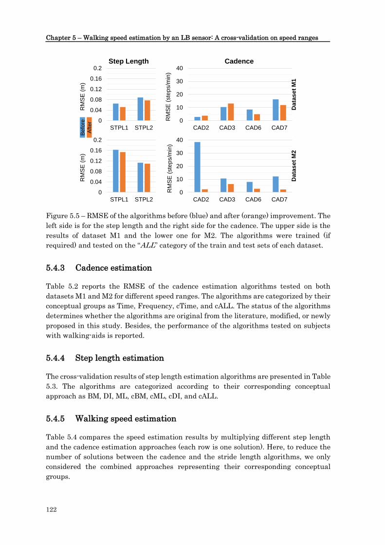
Chapter 5 – Walking speed estimation by an LB sensor: A cross-validation on speed ranges
122
Figure 5.5 – RMSE of the algorithms before (blue) and after (orange) improvement. The
left side is for the step length and the right side for the cadence. The upper side is the
results of dataset M1 and the lower one for M2. The algorithms were trained (if
required) and tested on the “ALL” category of the train and test sets of each dataset.
5.4.3 Cadence estimation
Table 5.2 reports the RMSE of the cadence estimation algorithms tested on both
datasets M1 and M2 for different speed ranges. The algorithms are categorized by their
conceptual groups as Time, Frequency, cTime, and cALL. The status of the algorithms
determines whether the algorithms are original from the literature, modified, or newly
proposed in this study. Besides, the performance of the algorithms tested on subjects
with walking-aids is reported.
5.4.4 Step length estimation
The cross-validation results of step length estimation algorithms are presented in Table
5.3. The algorithms are categorized according to their corresponding conceptual
approach as BM, DI, ML, cBM, cML, cDI, and cALL.
5.4.5 Walking speed estimation
Table 5.4 compares the speed estimation results by multiplying different step length
and the cadence estimation approaches (each row is one solution). Here, to reduce the
number of solutions between the cadence and the stride length algorithms, we only
considered the combined approaches representing their corresponding conceptual
groups.
Da
tas
et
M1
Data
se
t M
2
0
10
20
30
40
CAD2 CAD3 CAD6 CAD7
RM
SE
(ste
ps/m
in)
0
0.04
0.08
0.12
0.16
0.2
STPL1 STPL2
RM
SE
(m
)
0
10
20
30
40
CAD2 CAD3 CAD6 CAD7
RM
SE
(ste
ps/m
in)
0
0.04
0.08
0.12
0.16
0.2
STPL1 STPL2
RM
SE
(m
)
Step Length Cadence
Be
fore
Aft
er

Part II – Algorithms Design and Validation
123
Table 5.2 – Performance of the cadence estimation algorithms tested on different speed
ranges for both datasets M1 and M2. Here, cTime and cALL are combined approaches.
Column “Status” indicates if the algorithms are original, modified, or new. All Values
are also RMSE in steps/min.
Approach Algorithm Status Slow Normal Fast ALL Walking-aids
Data
set
M1
Time CAD1 Original 13.1 5.1 7.2 8.3 19.9
CAD2 Modified 2.1 5.4 1.9 3.8 12.1
CAD3 Modified 13.8 17.8 2.1 13.1 25.8
CAD4 Original 2.8 3.0 1.9 2.6 42.8
CAD5 Original 9.6 5.6 6.3 6.9 38.9
CAD6 Modified 3.8 5.4 4.8 4.9 15.7
Frequency CAD7 Modified 2.3 5.8 18.4 11.9 16.3
cTime CAD1-6 New 3.9 4.0 2.7 3.6 14.3
cALL CAD1-7 New 3.4 3.5 3.4 3.5 13.7
Data
set
M2
Time CAD1 Original 14.9 23.1 0.6 17.0 12.3
CAD2 Modified 2.8 1.3 2.0 2.4 27.6
CAD3 Modified 7.9 1.6 1.9 6.3 13.6
CAD4 Original 23.5 2.6 0.9 18.7 43.9
CAD5 Original 13.8 19.1 0.8 14.9 23.0
CAD6 Modified 3.3 1.6 1.5 2.8 30.4
Frequency CAD7 Modified 2.5 1.8 0.5 2.2 26.1
cTime CAD1-6 New 6.6 4.4 1.3 5.8 19.6
cALL CAD1-7 New 5.8 3.8 1.1 5.0 19.8

Chapter 5 – Walking speed estimation by an LB sensor: A cross-validation on speed ranges
124
Table 5.3 – Cross-validation results for the step length algorithms. Here, cBM, cML,
cDI, and cALL are combined approaches. Columns separated by the vertical lines
correspond to the training conditions. “S”, “N”, “F”, “A”, and “WA” report RMSE (in m)
of testing on Slow, Normal, Fast, ALL, and with walking-aids walkers. Column “Stat”
shows if the algorithms are original, modified, or new in this study. “App” means
Application. Column “Alg” refers to Algorithm, showing the number of each algorithm
(CADX).
Training condition Slow walkers Normal walkers Fast walkers ALL
App Alg Stat S N F A WA S N F A WA S N F A WA S N F A WA
Data
set
M1
BM 1 Mod. 0.15 0.16 0.19 0.17 0.10 0.05 0.06 0.04 0.05 0.22 0.06 0.10 0.10 0.09 0.28 0.05 0.06 0.04 0.05 0.21
2 Mod. 0.12 0.15 0.23 0.18 0.10 0.06 0.06 0.09 0.07 0.21 0.09 0.09 0.08 0.09 0.24 0.05 0.05 0.11 0.08 0.18
3 Orig. 0.11 0.12 0.20 0.15 0.10 0.06 0.09 0.08 0.08 0.18 0.07 0.10 0.08 0.09 0.20 0.05 0.07 0.09 0.07 0.16
4 Orig. 0.11 0.13 0.21 0.16 0.10 0.06 0.08 0.09 0.08 0.19 0.08 0.10 0.09 0.09 0.21 0.06 0.07 0.10 0.08 0.17
DI 5 New 0.13 0.17 0.26 0.21 0.09 0.09 0.06 0.10 0.08 0.26 0.18 0.10 0.09 0.12 0.34 0.08 0.05 0.13 0.09 0.24
6 New 0.08 0.20 0.39 0.27 0.14 0.09 0.05 0.10 0.08 0.28 0.17 0.09 0.08 0.11 0.34 0.09 0.05 0.10 0.08 0.27
7 New 0.13 0.16 0.22 0.18 0.11 0.05 0.06 0.06 0.06 0.22 0.08 0.09 0.07 0.08 0.27 0.04 0.05 0.07 0.06 0.21
ML 8 Orig. 0.07 0.12 0.24 0.17 0.15 0.11 0.14 0.18 0.15 0.20 0.21 0.18 0.10 0.16 0.54 0.09 0.10 0.12 0.10 0.32
9 Orig. 0.15 0.44 0.65 0.49 0.18 0.13 0.08 0.12 0.11 0.27 0.19 0.11 0.10 0.13 0.34 0.12 0.17 0.18 0.16 0.18
10 Orig. 0.06 0.27 0.22 0.22 0.17 0.06 0.10 0.13 0.11 0.33 0.15 0.10 0.05 0.10 0.36 0.07 0.16 0.08 0.12 0.18
11 Orig. 0.32 0.30 0.35 0.32 0.20 0.09 0.06 0.09 0.08 0.31 0.14 0.09 0.08 0.10 0.33 0.09 0.18 0.07 0.13 0.19
12 New 0.15 0.19 0.17 0.17 0.15 0.07 0.08 0.08 0.08 0.29 0.13 0.12 0.07 0.10 0.41 0.08 0.13 0.10 0.11 0.15
cBM 1-4 New 0.12 0.14 0.21 0.17 0.10 0.05 0.06 0.07 0.07 0.20 0.07 0.09 0.08 0.08 0.23 0.04 0.05 0.08 0.06 0.18
cDI 5-7 New 0.11 0.18 0.29 0.21 0.10 0.08 0.05 0.08 0.07 0.25 0.14 0.09 0.07 0.10 0.31 0.07 0.05 0.10 0.07 0.24
cML 8-12 New 0.13 0.15 0.13 0.14 0.15 0.07 0.05 0.09 0.07 0.26 0.16 0.10 0.05 0.11 0.39 0.06 0.12 0.07 0.09 0.18
cALL 1-12 New 0.08 0.13 0.18 0.15 0.12 0.06 0.05 0.08 0.06 0.24 0.13 0.09 0.06 0.09 0.32 0.05 0.08 0.07 0.07 0.18
Data
set
M2
BM 1 Mod. 0.15 0.13 0.08 0.14 0.16 0.18 0.11 0.06 0.15 0.18 0.20 0.10 0.06 0.17 0.20 0.18 0.11 0.06 0.15 0.18
2 Mod. 0.11 0.10 0.06 0.11 0.13 0.13 0.09 0.05 0.11 0.15 0.13 0.08 0.05 0.11 0.15 0.12 0.09 0.05 0.11 0.14
3 Orig. 0.13 0.10 0.05 0.11 0.10 0.13 0.09 0.05 0.11 0.10 0.14 0.08 0.05 0.12 0.11 0.13 0.08 0.05 0.11 0.10
4 Orig. 0.12 0.11 0.05 0.11 0.10 0.12 0.10 0.05 0.11 0.10 0.12 0.10 0.05 0.11 0.10 0.12 0.10 0.05 0.11 0.10
DI 5 New 0.10 0.09 0.15 0.10 0.15 0.15 0.04 0.07 0.12 0.21 0.20 0.08 0.02 0.16 0.27 0.15 0.04 0.07 0.12 0.21
6 New 0.11 0.10 0.13 0.11 0.17 0.15 0.04 0.07 0.12 0.22 0.21 0.07 0.03 0.17 0.29 0.16 0.06 0.05 0.14 0.25
7 New 0.10 0.12 0.10 0.11 0.13 0.12 0.09 0.07 0.11 0.16 0.13 0.09 0.07 0.11 0.17 0.12 0.09 0.07 0.11 0.16
ML 8 Orig. 0.10 0.13 0.15 0.11 0.19 0.12 0.08 0.11 0.11 0.19 0.17 0.07 0.02 0.14 0.21 0.11 0.05 0.09 0.10 0.14
9 Orig. 0.11 0.12 0.15 0.12 0.12 0.17 0.06 0.08 0.14 0.23 0.21 0.08 0.02 0.17 0.27 0.15 0.08 0.06 0.13 0.17
10 Orig. 0.09 0.09 0.20 0.11 0.21 0.22 0.04 0.12 0.18 0.34 0.27 0.15 0.03 0.23 0.44 0.12 0.07 0.03 0.10 0.13
11 Orig. 0.12 0.15 0.13 0.13 0.22 0.24 0.08 0.14 0.20 0.38 0.35 0.16 0.03 0.29 0.51 0.14 0.06 0.07 0.12 0.23
12 New 0.12 0.14 0.17 0.13 0.22 0.37 0.28 0.15 0.33 0.58 0.25 0.11 0.04 0.21 0.35 0.18 0.07 0.06 0.15 0.22
cBM 1-4 New 0.12 0.11 0.06 0.12 0.12 0.14 0.10 0.05 0.12 0.13 0.14 0.09 0.05 0.12 0.14 0.13 0.10 0.05 0.12 0.13
cDI 5-7 New 0.10 0.10 0.12 0.10 0.14 0.13 0.05 0.06 0.11 0.19 0.17 0.06 0.03 0.14 0.23 0.14 0.06 0.06 0.11 0.20
cML 8-12 New 0.09 0.11 0.14 0.10 0.18 0.25 0.12 0.12 0.21 0.37 0.23 0.10 0.02 0.19 0.33 0.13 0.06 0.05 0.11 0.17
cALL 1-12 New 0.10 0.11 0.11 0.10 0.15 0.17 0.05 0.07 0.14 0.25 0.18 0.06 0.03 0.15 0.24 0.13 0.07 0.05 0.11 0.16

Part II – Algorithms Design and Validation
125
Table 5.4 – Cross-validation results for the speed estimation. Here, each row represents
one solution to compute the speed. Columns separated by the vertical lines correspond
to training conditions. All values are RMSE in m/s. Besides, “STPL”, “CAD”, and “Freq”
refer to the step length, cadence, and frequency. For more information, refer to the
caption of Table 5.3.
Training
Condition Slow walkers Normal walkers Fast walkers ALL
STPL CAD S N F A WA S N F A WA S N F A WA S N F A WA
Data
set
M1
cBM cTime 0.22 0.29 0.41 0.33 0.17 0.10 0.15 0.15 0.14 0.34 0.14 0.21 0.18 0.19 0.40 0.09 0.12 0.16 0.13 0.32
Freq 0.21 0.28 0.51 0.37 0.19 0.10 0.16 0.31 0.22 0.34 0.15 0.23 0.31 0.25 0.39 0.09 0.14 0.32 0.22 0.32
cALL 0.22 0.29 0.42 0.33 0.17 0.10 0.15 0.17 0.15 0.34 0.14 0.21 0.19 0.19 0.39 0.09 0.12 0.18 0.14 0.31
cDI cTime 0.20 0.37 0.59 0.44 0.17 0.15 0.11 0.16 0.14 0.43 0.28 0.20 0.15 0.20 0.52 0.13 0.11 0.19 0.15 0.40
Freq 0.19 0.36 0.66 0.47 0.19 0.16 0.13 0.32 0.22 0.42 0.29 0.22 0.31 0.27 0.51 0.14 0.12 0.34 0.23 0.40
cALL 0.20 0.37 0.60 0.44 0.17 0.15 0.11 0.17 0.15 0.42 0.28 0.20 0.16 0.21 0.52 0.13 0.11 0.20 0.15 0.40
cML cTime 0.26 0.33 0.27 0.29 0.28 0.14 0.11 0.18 0.15 0.43 0.31 0.22 0.12 0.22 0.64 0.12 0.28 0.14 0.21 0.31
Freq 0.26 0.34 0.38 0.34 0.25 0.15 0.13 0.33 0.23 0.43 0.33 0.24 0.29 0.28 0.62 0.12 0.30 0.29 0.27 0.29
cALL 0.26 0.33 0.28 0.29 0.28 0.14 0.11 0.20 0.16 0.43 0.31 0.22 0.13 0.22 0.64 0.12 0.28 0.15 0.21 0.30
cALL cTime 0.15 0.28 0.36 0.29 0.21 0.13 0.12 0.15 0.13 0.40 0.25 0.21 0.13 0.19 0.54 0.10 0.18 0.14 0.15 0.32
Freq 0.15 0.28 0.47 0.34 0.20 0.13 0.13 0.31 0.22 0.40 0.26 0.23 0.30 0.26 0.52 0.11 0.19 0.30 0.23 0.31
cALL 0.15 0.28 0.37 0.30 0.21 0.13 0.12 0.16 0.14 0.40 0.25 0.21 0.14 0.20 0.53 0.10 0.18 0.15 0.15 0.32
Data
set
M2
cBM cTime 0.21 0.20 0.12 0.20 0.24 0.24 0.18 0.10 0.21 0.27 0.25 0.17 0.10 0.22 0.28 0.23 0.18 0.10 0.21 0.26
Freq 0.22 0.18 0.11 0.20 0.26 0.24 0.16 0.10 0.21 0.28 0.26 0.16 0.11 0.22 0.29 0.24 0.16 0.10 0.21 0.28
cALL 0.21 0.19 0.11 0.20 0.24 0.24 0.18 0.10 0.21 0.26 0.25 0.17 0.10 0.22 0.28 0.24 0.18 0.10 0.21 0.26
cDI cTime 0.15 0.18 0.27 0.18 0.30 0.22 0.11 0.13 0.19 0.37 0.28 0.13 0.07 0.23 0.43 0.22 0.12 0.13 0.19 0.38
Freq 0.16 0.16 0.26 0.17 0.32 0.23 0.09 0.12 0.19 0.39 0.28 0.12 0.07 0.24 0.45 0.23 0.10 0.12 0.19 0.40
cALL 0.15 0.18 0.27 0.17 0.30 0.22 0.10 0.13 0.19 0.36 0.28 0.12 0.07 0.23 0.43 0.22 0.12 0.12 0.19 0.38
cML cTime 0.15 0.20 0.31 0.18 0.35 0.37 0.17 0.27 0.31 0.63 0.37 0.17 0.05 0.31 0.58 0.21 0.11 0.12 0.18 0.33
Freq 0.16 0.18 0.30 0.18 0.38 0.37 0.21 0.26 0.32 0.67 0.37 0.19 0.05 0.31 0.60 0.23 0.10 0.11 0.19 0.36
cALL 0.15 0.20 0.30 0.18 0.35 0.37 0.17 0.27 0.31 0.63 0.37 0.17 0.05 0.30 0.58 0.22 0.11 0.12 0.18 0.33
cALL cTime 0.16 0.19 0.23 0.18 0.30 0.27 0.09 0.16 0.22 0.45 0.30 0.13 0.06 0.24 0.45 0.22 0.13 0.10 0.19 0.32
Freq 0.17 0.17 0.22 0.18 0.33 0.27 0.10 0.15 0.23 0.48 0.30 0.13 0.07 0.25 0.47 0.22 0.11 0.10 0.19 0.34
cALL 0.16 0.19 0.23 0.18 0.30 0.27 0.09 0.16 0.22 0.45 0.30 0.13 0.06 0.24 0.44 0.22 0.13 0.10 0.19 0.32

Chapter 5 – Walking speed estimation by an LB sensor: A cross-validation on speed ranges
126
5.5 Discussion
In this study, we implemented, improved, and compared several LB sensor-based
algorithms to estimate cadence, step length, and walking speed. We analyzed data from
two datasets, M1 (with the instrumented walkway) and M2 (with the IMU-based
reference system), containing both healthy and diseased populations (i.e., PD, MS, HE,
HD, OA). As shown in Table 5.1, the participants of both datasets have been distributed
uniformly among different speed ranges for both training and test sets. While the
patients fell mainly in slow and normal categories, the healthy ones were mainly in
normal and fast groups. Several people with walking-aids (32 subjects) were included
to test the algorithms’ performance under this unique situation.
Figure 5.5 illustrates that the proposed enhancements led to improved cadence and
step length estimation on both datasets M1 and M2. For the algorithms CAD2 and
CAD3 (both TD), while RMSE substantially decreased on dataset M2 (by at least 50 %),
a slight increase (maximum 25 %) was observed on dataset M1. One possible reason for
this observation is that the step-related peaks in M2 were generally weaker than in M1
(probably due to MS disease). That is why the proposed peak enhancement method was
generally more effective on the M2 dataset than M1. Moreover, the FD
algorithm(CAD7) reached a considerable improvement (minimum 30 %)) on both
datasets. For the step length algorithms (STPL1 and STPL2, both based on BM), the
error has been consistently reduced on both datasets M1 (minimum 16 %) and M2
(minimum 10 %).
Referring to Table 5.2, for the normal walkers, almost all cadence algorithms worked
properly and similar (an average RMSE of 3.5 and 3.8 steps/min on M1 and M2).
However, for the slow walkers, the TD algorithms showed a severe degradation of the
performance (up to an error of 13 and 23 steps/min on M1 and M2, respectively)
probably due to weakened step-related peaks in the acceleration signal. On the other
hand, the FD algorithm (CAD7) achieved an excellent error of 2.5 steps/min for slow
walkers on both datasets, possibly because this approach depends mainly on the gait-
related repetitive patterns than the peaks in the time domain signal.
Furthermore, for the fast walkers, while both approaches provided perfect results on
the M2 dataset (maximum error of 2 steps/min), a significant increase of the error (up
to 18 steps/min) was observed for the FD algorithm on M1. One explanation is that,
compared to the slow and normal walking, the fast walking might generate more
harmonics in the spectrum of the acceleration, which could confuse the FD cadence
algorithm to find the correct dominant frequency. For walking-aids people, the RMSE
considerably increases up to an average RMSE of 14 and 20 steps/min on M1 and M2.
Considering all circumstances for the cadence estimation, every algorithm showed
several advantages and limitations, so that it is difficult and unreliable to choose only
one. Nevertheless, it was interesting to observe that the combined approaches provided
a stable and high performance in all conditions. For instance, the cALL achieved an

Part II – Algorithms Design and Validation
127
RMSE of 3.4, 3.5, 3.4, and 13.7 steps/min for slow, normal, fast, walking-aids walkers
on the M1 dataset. On M2 datasets, the results are as 5.8, 3.8, 1.1, 19.8 steps/min,
respectively.
Only a few previous studies have reported cadence estimation error. In (Paraschiv-
Ionescu et al., 2019), the cadence estimation has been evaluated on typically developed
and cerebral palsy children where mean and STD absolute errors vary between [0.5-2]
and [1.3-7.2] steps/min, respectively. The study (Fasel et al., 2017a) also has reported
a median [IQR] of 0.15 [−1.95 2.27] steps/min for the estimation of cadence on healthy
subjects and using wrist sensors. It should be noted that the performance of cadence
estimation could be affected by target populations, in-lab or real-world situations, the
definition of cadence, and the definition of error, which is different in every study.
Regarding the different training conditions (training for ML and tuning for the other
approaches) in Table 5.3, we realized that training on a specific range of speed might
not be necessarily the best choice even when testing was performed on the same speed
range (e.g., training on slow walkers and testing on the same group). The results
demonstrated that training on “ALL” (i.e., including people from all speed ranges) led
to better performance than other training conditions. One main reason might be that
more data with higher diversity were fed into the algorithms during training on “ALL”,
resulting in more generalized models.
Considering the column “training on ALL” of Table 5.3, for the slow walkers, the BM-
based algorithms showed slightly better performance (RMSE around 0.04 m on M1 and
0.13 m on M2). One reason might be that they are more dependent on biomechanically-
derived models than the intensity or gait-related-patterns of the acceleration signal (as
ML or DI). Therefore, even when the acceleration signal is weak or distorted due to the
slow walking, they could still accurately estimate the step length. While DI algorithms
seemed to perform slightly better for the normal walkers, all approaches provided good
performances (RMSE around 0.08 m). No big difference was observed among different
approaches for the fast walkers (RMSE around 0.07 m and 0.05 m on M1 and M2). For
the walking-aids walkers, we noticed a significant performance drop in all approaches
(RMSE around of 0.18 m). Nevertheless, ML and BM seemed to be more appropriate
for this type of walking since they offer a high generalization ability, making them
robust against the body's atypical movement. Like cadence estimation, the combined
step length estimation approaches (cALL) appeared to be more accurate and robust for
all speed categories as well as the walking-aids group. On the M1 dataset, the combined
approach (i.e., cALL) achieved RMSE of 0.05, 0.08, 0.07, and 0.18 m for slow, normal,
fast, and walking-aids walkers, respectively. On M2 datasets its results are as 0.13,
0.07, 0.05, and 0.16 m, respectively.
Table 5.4 shows promising results for the estimation of walking speed. Like the step
length estimation, training on “ALL” walkers generally resulted in a better
performance. For slow walkers of dataset M1, the choice of cBM (BM-based combined
algorithm) or cALL with any cadence algorithms (i.e., cTime, Frequency, or cALL)

Chapter 5 – Walking speed estimation by an LB sensor: A cross-validation on speed ranges
128
achieved a better estimation of the speed (RMSE around 0.10 m/s). However, on M2, all
possible solutions resulted in the same RMSE around 0.22 m/s.
Furthermore, for the normal walkers of M1, the combination of cDI or cBM with any
cadence algorithms led to better performance (RMSE around 0.12 m/s). On M2,
however, the selection of cDI or cML with any cadence algorithms resulted in better
performance (RMSE around 0.12 m/s). Moreover, for the fast walkers, excluding the
combination of the FD cadence approach with any step length algorithms in M1, the
rest of the possibilities showed the same performance (RMSE around 0.14 m/s and 0.10
m/s on M1 and M2).
For the walking-aids group of M1, except the combination of DI with any cadence
algorithms, other combinations led to a similar RMSE around 0.32 m/s. However, on
M2, the combination of cBM with any cadence algorithms showed better performance
(RMSE around 0.27 m/s). Finally, Table 5.4 demonstrates that the choice of cALL for
both step length and cadence led to a more robust and acceptable estimation of the
speed in all conditions. This solution achieved an RMSE of 0.10, 0.18, 0.15, and 0.32
m/s for slow, normal, fast, and walking-aids walkers, respectively, on the M1 dataset.
Besides, it reached RMSE of 0.22, 0.13, 0.10, and 0.32 m/s on M2 dataset.
Looking at the literature, (McGinnis et al., 2017) achieved an RMSE of [0.12-0.15] m/s
to estimate speed on healthy and MS populations. A median absolute error of 0.3 m/s
was also reported in (Park et al., 2012) to estimate walking speed on a healthy
population. In (Soltani et al., 2019), a median [IQR] error of 0.10 [0.07 0.12] m/s was
obtained for the non-personalized wrist-based speed estimation on healthy population
in real-life situations.
For cadence, step length, and walking speed estimation, a slight difference was
observed between the results obtained on dataset M1 (with the instrumented walkway)
and M2 (with the IMU-based reference system). Generally speaking, dataset M2
seemed to be more challenging for the algorithms than M1. One reason might be that
the IMU-based reference system of M2 had higher error than the instrumented
walkway in M1. Another error source might be using a fixed height value (i.e., 170 cm)
in dataset M2, which is needed for some algorithms. Besides, detecting walking bouts
of M1 is more reliable than M2 (due to using the instrumented mat as reference).
The same analysis could be performed on bigger datasets recorded for long-durations
in daily-life situations as future work. This real-world analysis could prepare a wide
variety of challenging situations (self-triggered, purposeful, and multitasking walking
in a rich behavioral context) to test and judge the algorithms’ performance. For further
improvement, one possibility is to deploy a weighted average instead of an equally-
weighted one to optimize the performance of the combined algorithms by tuning the
weights (giving more weights to more accurate algorithms). For instance, it would be
possible to use the linear least square method to compute the optimal weights on a

Part II – Algorithms Design and Validation
129
tuning dataset. Moreover, comparing the error between healthy and pathological
populations could be another potential future work.
Furthermore, some of the TD cadence algorithms could be used for step demarcation
(timing of IC) in a fully autonomous LB-based speed estimation pipeline. This study
focused on evaluating speed estimation and its related parameters (i.e., cadence and
step length). However, a prospective study could be performed to evaluate the step
demarcation error to complete previous studies like the one presented in (Iijima and
Takahashi, 2020).
5.6 Conclusion
In this study, we developed several LB-worn IMU-based algorithms to estimate
cadence, step length, and, eventually, the walking speed. In most cases, the proposed
enhancements were useful for cadence (30-50 %) and step length (10-16 %) estimation.
The results showed that training on all people with different preferred speed led to
better performance.
For the slow walkers, the FD cadence estimation (RMSE of 2.5 steps/min), the BM-
based step length estimation (RMSE around 0.04 m on M1 and 0.13 m on M2), and
speed estimation by choosing cBM or cALL with any cadence algorithms (RMSE around
0.10 m/s on M1 and 0.22 m/s on M2) offered better performance. For normal walkers,
both cadence approaches (RMSE around 3.5 and 3.8 steps/min on M1 and M2) and all
the step length approaches (RMSE around 0.08 m) were preferred. For the speed
estimation on M1, selecting cDI or cBM with any cadence algorithms led to better
performance (RMSE around 0.12 m/s). On M2, however, opting cDI or cML with any
cadence algorithms showed more promising results (RMSE around 0.12 m/s).
Furthermore, for fast walkers, the TD cadence estimation (RMSE around 2.3 and 1.3
steps/min on M1 and M2), all the step length approaches (RMSE around 0.07 m and
0.05 m on M1 and M2), and all possible speed solutions, excluding the selection of FD
approach with any step length algorithms on M1, (RMSE around 0.14 m/s and 0.10 m/s
on M1 and M2), were suggested. The error significantly increased for people with
walking-aids where an RMSE around 14 steps/min, 0.18 m, and 0.27 m/s were observed
for estimating cadence, step length, and speed. The results demonstrated that the
combined approaches offer more robust solutions under various circumstances. For
instance, the combined speed estimation approach (cALL) achieved an RMSE of 0.10,
0.18, 0.15, and 0.32 m/s for slow, normal, fast, and walking-aids walkers, respectively,
on the M1 dataset. Besides, the results were 0.22, 0.13, 0.10, and 0.32 m/s on M2
dataset.

Chapter 5 – Walking speed estimation by an LB sensor: A cross-validation on speed ranges
130
5.7 Acknowledgments
The present study was performed in the framework of project Mobilise-D funding from
the Innovative Medicines Initiative 2 Joint Undertaking under grant agreement No
820820. This Joint Undertaking receives support from the European Union’s Horizon
2020 research and innovation program and EFPIA. We would like to thank all
consortium members, especially the technical validation work package (WP2). We also
thank Elisa Pelosin (from the University of Genova) for sharing the dataset M1. Finally,
we appreciate all the participants and medical centers’ staff for taking part in our
measurements.

131
Part III –
Real-world Application


133
6 Real-world gait speed estimation in
a large cohort: frailty and handgrip
strength1
6.1 Abstract
Real-world gait speed (GS2) is recognized as “the sixth vital sign” and is a key to
characterize people’s health status. A few previous studies used IMU in large clinical
cohort studies, but they mainly analyzed PA intensity (e.g., low, medium, vigorous)
rather than GS. One reason might be the difficulties of accurate estimation of GS in
real-world situations. Therefore, in this study, we demonstrated 1) the feasibility of
deploying a wrist-worn IMU-based system to assess GS in free-living situations; 2) the
meaningfulness of using GS in frailty/handgrip strength estimation. This study
included 2809 (1508 women; +45 y) participants. PA was measured using a wrist-worn
accelerometer. GB were stratified into three duration categories (<30; [30-120]; >120
seconds). Different GS measures of each category were used for analyses. Univariate
analysis was performed to investigate the effect of sociodemographic and lifestyle
factors on GS. Besides, we performed multivariate analyses to demonstrate the
advantage of adding GS as an independent prediction of frailty/handgrip strength
estimation. Compared to normative reference values in literature, similar speed values
and trends were observed. Using GS significantly improved frailty prediction and
handgrip strength estimation. The 95th PCT of GS and 30-120s duration provided the
highest discrimination power to distinguish subjects stratified by frailty or handgrip
strength. The methodology might be valuable in analyzing cohort datasets, and real-
world GS could be used as a reliable indicator of health and age-related functional
decline.
1 To be submitted as Soltani, A., Abolhassani, N., Marques-Vidal, P., Aminian, K., Vollenweider, P.,
Paraschiv-Ionescu, A., (2020), Real-world gait speed estimation and frailty/handgrip strength: a cohort-
based study, to American Journal of Epidemiology. Contributions are as follows: study design; data
cleaning; contribution to data analysis, performance evaluation and drafting the manuscript.
2 The abbreviation “GS” is used exclusively in chapter 6

Chapter 6 – Real-world gait speed estimation in a large cohort: frailty and handgrip strength
134
Keywords: gait speed, cohort studies, wearable systems, frailty, aging, obesity, PA, GB
duration.
6.2 Introduction
GS, recognized as the “6th vital sign” (Fritz and Lusardi, 2009; Middleton et al., 2015),
is a valid, reliable, and sensitive measure of people’s functional ability, closely
associated with well-being, healthy aging, and survival in elderly populations (Choi et
al., 2011; Del Din et al., 2016a; Elble et al., 1991; Harada et al., 1995; van Iersel et al.,
2008; Rydwik et al., 2012; Steffen et al., 2002). GS allows for monitoring overall health,
assessing functional status, early detection of disease and age-related functional
decline (e.g., frailty status (Cesari et al., 2016)), and for objectively quantifying the
impact of treatments and interventions (Castell et al., 2013; Fritz and Lusardi, 2009;
Maki, 1997; Middleton et al., 2015; Perera et al., 2015; Quach et al., 2011; Rochat et al.,
2010; Salarian et al., 2004; Studenski et al., 2011; Weiss et al., 2014). Most studies that
have contributed to the accumulated evidence about the reliability of GS as the
predictor of adverse health outcomes among community-dwelling adults were based on
measurements in the laboratory or clinical settings. However, mounting evidence has
indicated that the GS assessed in a laboratory setting does not fully reflect the GS of
the individuals in their everyday life context. Therefore, there is growing consensus to
develop a better way to assess gait in real-world conditions (Kawai et al., 2020;
Takayanagi et al., 2019; Van Ancum et al., 2019).
GS could be estimated in real-life situations by algorithms developed using multiple or
single IMU worn on different body segments (Paraschiv-Ionescu et al., 2004; Yang and
Li, 2012). PA in everyday life has multiple dimensions. Therefore, innovative
approaches have been developed and validated to extract metrics related to the type
(e.g., walking/running, body postures), duration of bouts, and intensity (e.g., GS,
accelerometer counts, metabolic equivalent of task) of PA. The most common sensor
locations for long-term monitoring are the trunk (e.g., waist, chest, hip, LB) or the wrist.
While the classification of multiple dimensions of PA (type, intensity, duration) using
the wrist-recorded data (e.g., acceleration) is technically challenging, recent research
focused on the development and validation of robust algorithms (Godfrey et al., 2008;
Lee et al., 2019; Rosenberger et al., 2016; Soltani et al., 2019, 2020; Troiano et al., 2014).
Given the difficulty of an accurate estimation of GS in real-world situations, most
existing commercial wearable devices deploy a more straightforward classical approach
for PA assessment by providing only an estimation of PA intensity levels (time spent in
sedentary, light, moderate, and vigorous intensities). Here, the issue is that the
processing of raw data (acceleration signal) and the definition of the thresholds used to
classify PA intensity levels differ between devices. Therefore, comparing PA-outcome
measures across different studies is not very trivial (Ward et al., 2005).

Part III – Real-world Application
135
Assessing PA by GS might overcome this issue since the gait characterized by the speed
is an “invariant” component of PA. Nevertheless, additional aspects should be
considered when using real-world GS as a PA outcome measure (Graham et al., 2008;
Kim et al., 2016). One important aspect is that the statistical metrics (e.g., mean,
median, mode, STD), derived from GS within different GB durations (e.g., short,
medium, long), have been rarely investigated in large clinical cohort studies (Pradeep
Kumar et al., 2020). However, identifying GB durations, probably corresponding to
various “purposeful” daily activities that represent a person’s physical capacity, is an
essential topic for outcome evaluation in population-based studies. Additional aspects
are the potential influence of external/contextual factors on GS, increasing the
intra/inter subjects’ variability. For instance, although PA features are subject to
ultradian and circadian changes so that they should be studied during the whole 24
hours activity cycle (Carlson et al., 2012; Firmann et al., 2008; Rosenberger et al., 2016),
only a few studies addressed this aspect (Cabanas-Sánchez et al., 2020; Hillel et al.,
2019). Another critical aspect is the small sample size of many studies, limiting the
statistical analyses power and reliability to generalize the results for large populations.
Finally, the complexity of the systems for PA objective assessment (e.g., multiple body-
worn IMU) could affect people’s daily habits, reducing compliance for participating in
long-term monitoring protocols (Buchser et al., 2005). The complexity also necessitates
additional technical considerations (e.g., synchronization of devices) which could
impose time and money costs.
This study pursues two main goals. First, we aim at the feasibility of assessing GS
using an accurate, easy-to-use wrist-worn IMU-based system (Soltani et al., 2019, 2020)
in a large population (more than 2800 participants) for a long-duration measurement
(13 consecutive days, 24 hours per day) in free-living conditions. Second, we seek the
added values of including the real-world GS to estimate clinical outcomes such as frailty
and handgrip strength. Also, we investigate the association between the GS and
subjects’ characteristics (e.g., demographic information). As a secondary outcome, we
report what GS metric and in what GB duration provides the highest discrimination
power to distinguish between different groups of people stratified by clinical indexes
such as frailty and handgrip strength.
6.3 Methods
6.3.1 Study population
Subjects were enrolled in the framework of the CoLaus3 cohort study. The Colaus study
is an ongoing prospective survey, investigating the biological and genetic determinants
of cardiovascular risk factors and cardiovascular disease in the population of Lausanne,
Switzerland. The detailed description of the CoLaus study and its follow-ups has been
3 https://www.colaus-psycolaus.ch/

Chapter 6 – Real-world gait speed estimation in a large cohort: frailty and handgrip strength
136
reported elsewhere (Fried et al., 2001). A simple, non-stratified random sample of the
Lausanne population aged between 35 and 75 years was chosen based on the following
inclusion criteria: (i) written informed consent and (ii) willingness to take part in the
examination and to provide blood samples. The baseline survey was conducted between
2003 and 2006, the first follow-up between 2009 and 2012, and the second follow-up
between 2014 and 2017. The baseline and subsequent follow-ups included an interview,
a physical exam, blood sampling, and questionnaires. In the second follow-up (4881
participants), daily PA was also assessed by accelerometry. Hence, data from the second
follow-up was used. It should also be noted that we excluded the participants whose GS
metrics or other covariates data were missing.
6.3.2 PA measurement
Participants wore a 3-axial accelerometer (GENEActiv Original, ActivInsights Ltd,
United Kingdom) on the right wrist for 13 successive full days in their free-living
situations without any supervision or intervention. The GENEActiv device is
lightweight (16 g), waterproof, and allows continuous measurement for a maximum of
45 days. The acceleration was recorded with a range of ±8 g and a sampling frequency
of 50 Hz (high enough to avoid ailiasing during gait analysis (Van Hees et al., 2014)),
where the accelerometer was calibrated based on (Sabia et al., 2014). After recording,
the raw acceleration data were transferred into a computer for analysis to identify the
GB and estimate GS using algorithms validated in chapters 3 and 4 of this thesis
(Soltani et al., 2019, 2020).
6.3.3 Real-world GB detection and speed estimation
Figure 6.1 illustrates the block diagram of the system deployed for the real-world GS
estimation using wrist acceleration signals.
Figure 6.1 – Block diagram of the system used for real-world GS estimation. Two
validated algorithms were used, one for GB detection (chapter 3, (Soltani et al., 2020))
and the second for GS estimation (chapter 4, (Soltani et al., 2019)).

Part III – Real-world Application
137
6.3.3.1 GB detection
The algorithm presented in chapter 3 (Soltani et al., 2020) was employed to detect GB.
In this algorithm, after decreasing noise by preprocessing the wrist acceleration,
several biomechanically meaningful features (defined based on intensity, periodicity,
posture, and noisiness) were extracted. The features were then fed into a classification
procedure consisting of a Bayes classifier followed by two smart post-classification
blocks. The output of this algorithm was per-second labels for continuous GB without
any breaks. A median sensitivity, specificity, accuracy, precision, and F1-score of 90.2,
97.2, 96.6, 80.0, and 82.6 are reported (all values in %, highest possible value for these
classification performance metrics is 100, corresponding to a full agreement between
the validated algorithm and the ground truth).
6.3.3.2 GS estimation
We used the non-personalized version of the algorithm proposed in (Soltani et al., 2019)
to estimate the GS of the GB detected in the previous step. In this algorithm, first, the
wrist acceleration signal was passed through a preprocessing stage to enhance the
meaningful features. Then, relevant features such as energy, cadence (step frequency),
mean of acceleration, mean of the jerk, intensity of wrist swing were extracted and fed
into a linear regression model to estimate the instantaneous speed (per second) of each
detected GB. A median RMSE of 0.10 and 0.31 m/s are reported for the instantaneous
walking and running speed estimation, respectively, using the non-personalized
version.
For each subject in this study, detected GB were stratified into three categories
according to their durations (<30s; [30-120]s; >120s). The main idea behind this
grouping was the fact that the short (<30s) bouts occur mostly indoors and are mainly
context-dependent, whereas the long (>120s) bouts happen mostly outdoors (Hickey et
al., 2016). The other category ([30-120]s) could be a mixture of indoor and outdoor
activities (Hickey et al., 2016). For each subject, we computed a set of speed metrics
derived from the statistical distribution of GS (average, mode, median, 75th, 90th, and
95th PCT, STD, and maximum) of each GB duration category.
6.3.3.3 Other covariates
We collected gender and age by questionnaire. Age was categorized into four groups:
[45-54], [55-64], [65-74] and [75 years. Height and weight were assessed by a Seca®
scale (Seca Gmb, Hamburg, Germany) with the participants in light clothes and
without shoes. BMI was categorized as normal (18.5< BMI <25 kg/m2), overweight (25≤
BMI <30 kg/m2) and obese (≥30 kg/m2). As the percentage of underweight (BMI≤ 18.5
kg/m2) participants was small (<2 %), they were included in the normal weight group.
Handgrip strength was assessed using the Baseline® Hydraulic Hand Dynamometer
(Fabrication Enterprises Inc, Elmsford, NY, USA) with the subject seated, shoulders

Chapter 6 – Real-world gait speed estimation in a large cohort: frailty and handgrip strength
138
adducted, and neutrally rotated, elbow flexed at 90°, forearm in a neutral position, and
wrist between 0 and 30° of dorsiflexion. Three measurements were performed
consecutively with the right hand, and the highest value was included in the analyses.
Frailty condition was defined using gender, BMI, and handgrip strength (kg) and
categorized as frail and non-frail according to Fried et al. (Fried et al., 2001). Therefore,
the frailty condition was identified as follows; for men: if BMI≤24 and handgrip strength
≤29 or 24<BMI≤28 and handgrip strength ≤30 or BMI>28 and handgrip strength ≤32;
and for women: if BMI≤23 and handgrip strength ≤17 or 23<BMI≤26 and handgrip
strength ≤17.3 or 26<BMI≤29 and handgrip strength ≤18 or BMI>29 and handgrip
strength ≤21.
PA intensity levels were estimated from the raw acceleration data using the R-package
GGIR4 (Sabia et al., 2014; Van Hees et al., 2014) and the criteria of White et al. (Tom
White, 2018) to define moderate and vigorous PA. PA levels were further categorized
into inactive (<150 min/week) and active (≥150 min/week) of moderate and vigorous PA,
respectively.
6.3.3.4 Ethical statement
The institutional Ethics Committee of the University of Lausanne, which afterward
became the Ethics Commission of Canton Vaud5, approved the baseline CoLaus study
(reference 16/03). The approval was renewed for the first (reference 33/09) and the
second (reference 26/14) follow-ups. The study was performed in agreement with the
Helsinki declaration and its former amendments, and under the applicable Swiss
legislation. All participants gave their signed informed consent before entering the
study.
6.3.3.5 Statistical analysis
Statistical analysis was performed using Stata software version 16.0 (Stata Corp,
College Station, TX, USA) and MATLAB (MathWorks, USA). First, we performed
univariate analysis to investigate the effect of each factor (gender, age, BMI, and PA
levels) on the GS and to demonstrate the consistency between the speed values
estimated in this study and the normative values in the literature. A comprehensive
multivariate analysis was then designed to show the advantage of adding real-world
GS to predict frailty condition and handgrip strength estimation. Both analyses are
briefly described as follows:
6.3.3.5.1 Univariate Analysis
We computed the average number of GB detected within each duration category for
different age groups to ensure having enough sample size within each group. Then, the
4 http://cran.r-project.org
5 www.cer-vd.ch

Part III – Real-world Application
139
subject’s preferred GS, for all GB as well as for GB in each duration category, was
estimated as the mode (peak) of PDF using the Kernel Smoothing Function (MATLAB
function “ksdensity”). Besides, the distributions of the preferred GS of subjects
stratified by gender, age, BMI, and PA levels were compared through boxplots to
highlight the effect of each factor on the preferred speed.
6.3.3.5.2 Multivariate Analysis
Two logistic regression models (A and B) were built to assess the importance of
including GS in predicting frailty condition. Model A included gender, age, BMI, and
PA intensity levels, as these covariates are associated with frailty (Fried et al., 2001).
Model B used the same covariates as model A, plus the GS metrics. Two linear
regression models assessed the association with handgrip strength: model A included
gender, age, BMI, and PA levels, and model B was the same as model A plus the GS
metrics. For both analyses, the results were expressed as the Area Under the ROC
(AUC) and Akaike’s and Bayesian information criteria (AIC and BIC, respectively). The
improvement in predicting frailty, as well as estimating handgrip strength, was
assessed by comparing model B with model A using the likelihood ratio test (LR) as well
as the AUC. Eventually, to confirm the results of the previous analyses, a stepwise
logistic regression (forward method) with a p-value for the entry of 0.05 was deployed
to select the speed metric(s) with the most vital relation with the non-frail condition.
The same analysis was performed for the handgrip strength with a stepwise linear
regression instead. Due to the large number of tests performed, statistical significance
was arbitrarily assessed for a two-sided test with p<0.001.
6.3.3.5.3 Sensitivity analyses
The system deployed in this study for GB detection and GS estimation (Figure 6.1)
could not distinguish between walking and running. Therefore, we excluded the
participants whose 95th PCT of speed was above the maximum value of walking speed
reported in (Bohannon, 1997). We then repeated the multivariate analysis as described
above. We used the 95th PCT of speed since, statistically, it is more reliable than the
maximum value.
6.4 Results
6.4.1 Selection of participants
Of the initial 4881 participants, 1982 (no walking speed data) and 90 (missing
covariates) were excluded, and 2809 (46.3 % men, 53.7 % women, mean age 62.4 ± 9.9
years) were included in this study. After analysis, each participant’s data was verified
to check the number of days with detected GB (valid days); days with no detected GB
were discarded. From the 2809 subjects, ~98 % of subjects had at least eight valid days,
including weekly and weekend days. This number was large enough to estimate

Chapter 6 – Real-world gait speed estimation in a large cohort: frailty and handgrip strength
140
preferred GS and related gait metrics (Soltani et al., 2017). Supplementary Table 6.1
reports the characteristics of the participants included and excluded in this study.
6.4.2 Real-world GS estimation
Figure 6.2 illustrates an example of the wrist acceleration-based GS estimation for one
participant of this study. Panel A displays the wrist acceleration norm and the GS
estimated during 13 continuous days in free-living situations. Panel B is a zoom on
Panel A to show the analysis results in a typical day (24h) in real-world situations.
Figure 6.2 demonstrates that the wrist-based method successfully estimated a
consistent GB sequence and their corresponding speed in regular daily life activity.
There is a clear repetitive pattern of GB among successive days. Each day starts with
a non-active period, likely related to sleep time, followed by two active periods in the
morning and the afternoon (probably associated with a daily routine). Moreover,
sometimes, a few GB could be observed in the evening. In many cases, the GS (i.e., the
intensity of activities) is higher in the morning and gradually decreases.
6.4.3 Univariate analysis
Figure 6.3 shows the GB distribution (mean and STD) for each age group within each
duration category, expressed as the percentage of the total number of GB detected for
each subject in each age group. The distributions of the GB appeared relatively similar
between the age groups. Figure 6.4 illustrates the preferred GS distribution for each
bout duration, using the pooled data from all subjects. The effect of subject-specific
factors (gender, age, BMI, PA level) on the preferred GS is graphically illustrated with
the boxplots in Figure 6.5.

Part III – Real-world Application
141
Figure 6.2 – An illustrative example of a real-world GS estimation for a representative
subject monitored in daily life situations. A) Estimated speed of detected GB (red) and
wrist acceleration norm (blue) during 13 continuous days. B) One typical day (day #12).

Chapter 6 – Real-world gait speed estimation in a large cohort: frailty and handgrip strength
142
Figure 6.3 – Distribution of the GB within each duration category, stratified by age
groups. Each bar and the corresponding error bar report the mean and STD of GB
within each duration category and each age group. The values were calculated as
percentages of their total number of GB for each individual in each age group.
Figure 6.4 – PDF of the preferred GS values for each GB duration, including data from
all subjects. First, the preferred speed of each subject for each bout duration was
computed. Then the PDF was estimated by the Kernel Smoothing Function (function
“ksdensity” in MATLAB).

Part III – Real-world Application
143
Figure 6.5 – Boxplots of the preferred (mode value of) speed of different groups stratified
by gender, age, BMI, and PA levels. Here, the green line connects each group’s median
value.
6.4.4 Multivariate analysis: frailty and handgrip strength estimation
The logistic regression model A (without GS metrics) and model B (with GS metrics) for
prediction of frailty were analyzed (Table 6.1). As indicated by a lower AIC/BIC and a
significant LR test, model B provides a substantial improvement in the prediction of
frailty condition by taking advantage of any speed metrics in all GB durations.
Compared to model A, the AUC, AIC, and BIC of model B were enhanced in all
conditions, where an average improvement of 3.1, 3.1, and 2.7 % are respectively
observed for all GS metrics in all GB durations (Table 6.1). However, the improvements
for the duration of 30-120s are slightly greater than the other periods. Moreover, the
LR test suggests GS’s 95th PCT as a proper speed metric in all GB durations to predict
frailty. Similar outcomes could be observed for estimating the handgrip strength (Table
6.2). Estimating the handgrip strength by model B, including any GS metrics in all GB
durations, leads to a significant improvement compared to model A. Similarly, the 95th
PCT of GS and GB duration 30-120s showed more promising results.
In order to visualize the difference between models A and B for the prediction of frailty,
the ROC curves of both models are presented (Figure 6.6). Here, we separated the
results in each GB duration, and only the baseline (model A) and three speed metrics
(mean, 90th, and 95th PCT) are displayed. Figure 6 also visually confirms these results
where the AUC of baseline (model A) in all GB durations is less than model B.
The results of the stepwise regression models using different GS metrics within
different GB duration categories in predicting non-frailty and handgrip strength are
presented in Table 6.3. The stepwise regression analysis results also support the
previous findings where the 95th PCT of the GS entered into the model in all GB
durations.

Chapter 6 – Real-world gait speed estimation in a large cohort: frailty and handgrip strength
144
Table 6.1 – Effect of adding speed metrics to predict frailty. Model A includes gender,
age, BMI, and PA. Model B consists of all variables from model A plus the variable of
interest (the speed metric specified in each row). “NaN” corresponds to the values which
were not possible to be computed.
Name Duration (s) Speed metrics AUC LR p-value AIC BIC
Model A Each duration None 0.763 NaN NaN 1497.4 1544.8
Model B < 30 Mode 0.781 41.26 <0.001 1458.1 1511.5
Median 0.789 58.62 <0.001 1440.8 1494.1
Mean 0.793 71.06 <0.001 1428.3 1481.7
75th PCT 0.789 60.28 <0.001 1439.1 1492.5
90th PCT 0.796 72.72 <0.001 1426.7 1480.0
95th PCT 0.798 77.27 <0.001 1422.1 1475.5
Maximum 0.782 40.34 <0.001 1459.1 1512.4
STD 0.781 31.74 <0.001 1467.6 1521.0
30-120 Mode 0.781 41.46 <0.001 1457.9 1511.3
Median 0.788 57.59 <0.001 1441.8 1495.2
Mean 0.793 68.59 <0.001 1430.8 1484.2
75th PCT 0.789 59.28 <0.001 1440.1 1493.5
90th PCT 0.795 70.06 <0.001 1429.3 1482.7
95th PCT 0.800 78.04 <0.001 1421.4 1474.7
Maximum 0.785 43.70 <0.001 1455.7 1509.1
STD 0.779 26.89 <0.001 1472.5 1525.9
> 120 Mode 0.778 28.28 <0.001 1471.1 1524.5
Median 0.785 38.60 <0.001 1460.8 1514.2
Mean 0.790 49.92 <0.001 1449.5 1502.8
75th PCT 0.785 38.49 <0.001 1460.9 1514.3
90th PCT 0.791 50.77 <0.001 1448.6 1502.0
95th PCT 0.795 58.76 <0.001 1440.6 1494.0
Maximum 0.770 15.46 <0.001 1483.9 1537.3
STD 0.774 17.07 <0.001 1482.3 1535.7

Part III – Real-world Application
145
Table 6.2 – Effect of adding the GS metrics to estimate the handgrip strength. Model A
includes gender, age, BMI, and PA. Model B consists of all variables from model A plus
the variable of interest (the speed metric specified in each row). “NaN” corresponds to
the values which were not possible to be computed.
Name Duration (s) Speed metrics AUC LR p-value AIC BIC
Model A Each duration None 0.669 NaN NaN 18780.5 18827.9
Model B < 30 Mode 0.684 100.91 <0.001 18681.6 18734.9
Median 0.690 210.80 <0.001 18571.7 18625.0
Mean 0.694 278.01 <0.001 18504.4 18557.8
75th PCT 0.690 234.44 <0.001 18548.0 18601.4
90th PCT 0.694 290.61 <0.001 18491.8 18545.2
95th PCT 0.696 309.43 <0.001 18473.0 18526.4
Maximum 0.685 112.55 <0.001 18669.9 18723.3
STD 0.681 135.30 <0.001 18647.2 18700.5
30-120 Mode 0.685 107.18 <0.001 18675.3 18728.6
Median 0.689 198.52 <0.001 18583.9 18637.3
Mean 0.693 257.77 <0.001 18524.7 18578.1
75th PCT 0.689 215.08 <0.001 18567.4 18620.7
90th PCT 0.694 260.00 <0.001 18522.5 18575.8
95th PCT 0.696 285.11 <0.001 18497.3 18550.7
Maximum 0.687 111.52 <0.001 18670.9 18724.3
STD 0.681 101.86 <0.001 18680.6 18734.0
> 120 Mode 0.681 91.90 <0.001 18690.6 18743.9
Median 0.686 170.34 <0.001 18612.1 18665.5
Mean 0.688 221.42 <0.001 18561.0 18614.4
75th PCT 0.685 159.97 <0.001 18622.5 18675.9
90th PCT 0.689 213.48 <0.001 18569.0 18622.3
95th PCT 0.691 220.24 <0.001 18562.2 18615.6
Maximum 0.677 66.16 <0.001 18716.3 18769.7
STD 0.679 53.03 <0.001 18729.4 18782.8

Chapter 6 – Real-world gait speed estimation in a large cohort: frailty and handgrip strength
146
Figure 6.6 – ROC of model A (baseline) and B (+mean, +90th, and +95th PCT) in
predicting frailty according to each bout duration.
Table 6.3 – Summary of results of the stepwise regression forward models for predicting
non-frailty and handgrip strength. Here, sign “-” refers to variables that did not remain
in the stepwise approach.
Speed metrics p-values for Non-frailty p-values for Handgrip strength
< 30 s 30-120 s > 120 s < 30 s 30-120 s > 120 s
Mode 0.048 - - - - -
Median - - - - - -
Mean - - - - - <0.001
75th PCT - - - - - <0.001
90th PCT - - - - - -
95th PCT <0.001 <0.001 <0.001 <0.001 <0.001 <0.001
Maximum 0.044 0.022 - - 0.006 -
STD - 0.018 - <0.001 <0.001 -

Part III – Real-world Application
147
6.4.5 Sensitivity analysis
The exclusion of participants with high speed (assumed as running) excludes 753 out
of 2809 subjects. The result of the repeated multivariate analysis for the remainder of
participants (2056 subjects) could be found in the Supplementary Table 6.1,
Supplementary Table 6.2, and Supplementary Table 6.3. The exclusion of running data
had no significant impact on the multivariate analyses; consequently, the same
outcomes can still be outlined.
6.5 Discussion
The results of this study demonstrated the feasibility of using a wrist acceleration-
based method for long-term monitoring of real-world GS in a large cohort of community-
dwelling adults. Moreover, the statistical analysis demonstrated that the real-world
GS’ distribution, estimated from the wrist-worn device, was consistent with normative
values published in the literature, when subjects were stratified by demographic data
such as gender, age, BMI, and daily PA levels (Bohannon, 1997; Bohannon and
Williams Andrews, 2011). Moreover, it also highlights that the statistical metrics
(mode, median, mean, 75th, 90th, 95th PCT, maximum, and STD) derived from the
distribution of GS within different bout durations improved the discriminative power
of regression models built for the prediction of frailty, and handgrip strength. The large
sample size (2809 subjects) and the uniform distributions of the subjects within each
category identified by gender, age, BMI, and PA allowed a comprehensive, valid
statistical analysis of the GS metrics.
6.5.1 Univariate analysis
As illustrated in Figure 6.4, the range of [1-1.6] m/s for the preferred GS (estimated as
the mode/peak of PDF), for each range of bout duration, is consistent with the values
reported by several previous studies (Bohannon and Williams Andrews, 2011).
Interestingly, the trend observed with age and gender is similar to recent data on a big
Japanese population-based cohort study, where the daily-life GS was assessed using
smartphone-integrated GNSS (Obuchi et al., 2020). Nevertheless, this technology
might raise privacy issues and might not be accepted by the ethical committee in
clinical research. Similarly, the percentage of the total GB number within each duration
range (see Figure 6.3) appeared to be similar to the previous studies (Del Din et al.,
2016a; Orendurff et al., 2008). It indicated an exponential reduction of the number of
GB for longer durations. From Figure 6.3, it could be observed that about 65 % were
short (<30s), 30 % were medium duration (30-120s), and only 5 % were long (>120s),
and this trend was similar for all age categories. It was also observed that longer GB
had a higher variation of GS. One explanation for this behavior would be that the long
GB was probably related to outdoor activities, which are more influenced by contextual
factors (e.g., quick utilitarian walk to a shop, or peaceful recreational walk in a park).

Chapter 6 – Real-world gait speed estimation in a large cohort: frailty and handgrip strength
148
An exact effect of gender, age, BMI, and PA levels on the preferred GS was observed.
The trends in Figure 6.5 are also consistent with the literature (Schimpl et al., 2011b)
and show the importance of real-world GS for monitoring and assessing functional
decline caused by factors such as aging and obesity.
6.5.2 Multivariate analysis
Our study demonstrated a significant improvement in predicting frailty and estimating
handgrip strength by taking advantage of any speed metrics in any GB durations.
However, the improvements appear slightly higher within the GB duration between
[30-120]s than the other durations. The possible explanation is that the short bouts
(<30s) are usually related to indoor activity, such as stepping in a constrained
environment during daily tasks. Hence, individuals are not necessarily challenged by
their walking ability. On the other side, the long bouts (>120s) represent only a small
percentage of daily GB. Therefore, their limited number of samples might reduce
statistical power. The medium-duration GB (30-120s) appear optimal for estimating
robust speed metrics because their number is sufficiently high (about 30 %), and the
duration long enough to correspond to a stable gait pattern.
Furthermore, the 95th PCT of the GS seems to be the best speed metric in all GB
durations to predict frailty. A Canadian study on older adults found that GS alone was
sensitive and specific as a proxy for the Fried frailty phenotype. However, the dual-trait
measure of GS with grip strength was more sensitive than individual traits and other
possible dual-factor combinations (Lee et al., 2017). A systematic review also concluded
that GS alone was as good as other composite tools in predicting the risk of adverse
outcomes. There was sufficient evidence to support the GS as a single-item assessment
tool for frailty screening in community-dwelling older adults (Abellan van Kan et al.,
2009). In our study, the significant difference between models A and B and increased
AUC for 95th PCT of GS in predicting the frailty revealed that this speed metric could
serve a better as a proxy for the frailty than other GS metrics. The explanation is that
the 95th PCT is an estimation of the upper-bound of GS distribution. Therefore this
metric is more likely to reflect the physical/physiological reserve of the person. Real-
world GS metrics also predicted handgrip strength. Clinically, these results were
expected and agreed with the existing studies (Alley et al., 2014; Nagamatsu et al.,
2019). Indeed, a reduction of both GS and handgrip strength might appear due to
muscle weakness, which is one of the cardinal signs of frailty/transition to frailty.
6.5.3 Strengths and limitations
The main strengths of this study are the assessment of GS in a long-duration
monitoring protocol (i.e., 13 successive full days), in a large (2809 participants) and
diverse cohort (i.e., gender, age, BMI), and under entirely free-living situations using
acceleration data from a wrist-worn device. The comprehensive statistical analyses on
such a rich database with a wide range of GS led to a better and more reliable

Part III – Real-world Application
149
understanding of the importance of GS in clinical applications. Furthermore, the
methodology presented could help analyze massive existing databases, recorded with
GENEActiv device or any other wrist-worn tools that record raw acceleration data
(Cabanas-Sánchez et al., 2020; Cassidy et al., 2018; Doherty et al., 2017; da Silva et al.,
2014). The technique could be valuable for assessment or screening of adverse
conditions in both clinical and epidemiological studies.
This study also has some limitations. First, it was conducted in a community-dwelling
population that could be considered mostly healthy. Therefore, the results might not
apply to hospitalized and impaired people. Second, frailty was defined using a small set
of criteria. There were an imbalanced number of subjects in the fit and frail groups; the
results might change if the definitions based on other criteria would be used.
Nevertheless, the definition of frailty used in this study is reliable in functional
performance (Fried et al., 2001). Third, this study was conducted in Lausanne, a steep
city, and the results might not be generalizable to other settings. Furthermore, the gait
definition included walking and eventually running activity; however, the sensitivity
analysis confirmed the same results. Finally, this study was cross-sectional where
causality between PA and frailty or handgrip strength cannot be established; the
ongoing follow-up of the CoLaus cohort will allow such assessment.
6.6 Conclusions
The current study demonstrated the feasibility of assessing real-world GS in extensive
cohort studies using a simple, unobtrusive wrist-worn device recording raw acceleration
data and algorithms developed and validated for this configuration. The methodology
could be valuable for analyzing existing cohort datasets. The results showed that real-
world GS could be a reliable indicator of health and age-related functional declines. It
could effectively improve the evaluation of frailty condition.
6.7 Acknowledgment
This study has been supported by the research grants from GlaxoSmithKline, the
Faculty of Biology and Medicine of Lausanne, and the Swiss National Science
Foundation (grants 33CSCO-122661, 33CS30-139468, and 33CS30-148401). We would
like to thank all participants and medical center staff who took part in our
measurements.

Chapter 6 – Real-world gait speed estimation in a large cohort: frailty and handgrip strength
150
6.8 Annex: Supplementary results
Supplementary Table 6.1 – Characteristics of participants included in this study.
Results are expressed as the number of participants (column percentage) or average
(STD). Inter-group comparisons performed using chi-square and student’s t-test.
Factors Categories Included Excluded
Total 2809 2072
Gender Men 1301 (46.3) 891 (43.0)
Women 1508 (53.7) 1181 (57.0)
Age (years) [45-54] 830 (29.6) 516 (24.9)
[55-64] 909 (32.4) 593 (28.6)
[65-75] 729 (25.9) 570 (27.5)
75+ 341 (12.1) 393 (19.0)
BMI Normal + underweight 1157 (41.2) 700 (33.8)
Overweight 1140 (40.6) 635 (30.6)
Obese 512 (18.2) 337 (16.3)
Missing data 0 (0) 400 (19.3)
Physically Active (PA) Active 1091 (38.8) 66 (3.2)
Inactive 1718 (61.2) 92 (4.5)
Missing data 0 (0) 1914 (92.3)
Frailty No 2552 (90.8) 1376 (66.4)
Yes 257 (9.2) 209 (10.1)
Missing data 0 (0) 487 (23.5)
Handgrip strength (kg) 34.4 ± 12.0 32.7 ± 12.2

Part III – Real-world Application
151
Supplementary Table 6.2 – Prediction of frailty after excluding participants with
possible excessive speed (running). Model A includes gender, age, BMI, and PA. Model
B consists of all variables from model A plus the variable of interest (the speed metric
specified in each row). “NaN” corresponds to the values which were not possible to be
computed.
Name Duration (s) Speed metrics AUC LR p-value AIC BIC
Model A Each duration None 0.775 NaN NaN 1099.1 1144.1
Model B < 30 Mode 0.783 23.74 <0.001 1077.4 1127.9
Median 0.790 35.23 <0.001 1065.9 1116.5
Mean 0.794 42.62 <0.001 1058.5 1109.1
75th PCT 0.790 34.22 <0.001 1066.9 1117.5
90th PCT 0.796 42.64 <0.001 1058.5 1109.1
95th PCT 0.798 45.86 <0.001 1055.3 1105.8
Maximum 0.783 20.75 <0.001 1080.4 1130.9
STD 0.783 13.67 <0.001 1087.5 1138.0
30-120 Mode 0.785 25.93 <0.001 1075.2 1125.8
Median 0.789 33.50 <0.001 1067.6 1118.2
Mean 0.794 40.95 <0.001 1060.2 1110.7
75th PCT 0.789 32.07 <0.001 1069.1 1119.6
90th PCT 0.795 38.99 <0.001 1062.1 1112.7
95th PCT 0.800 45.94 <0.001 1055.2 1105.8
Maximum 0.780 17.14 <0.001 1084.0 1134.6
STD 0.780 8.89 <0.001 1092.2 1142.8
> 120 Mode 0.783 15.85 <0.001 1085.3 1135.8
Median 0.788 23.50 <0.001 1077.6 1128.2
Mean 0.792 30.29 <0.001 1070.8 1121.4
75th PCT 0.787 22.49 <0.001 1078.6 1129.2
90th PCT 0.792 29.71 <0.001 1071.4 1122.0
95th PCT 0.795 34.71 <0.001 1066.4 1117.0
Maximum 0.774 4.05 <0.001 1097.1 1147.6
STD 0.778 6.23 <0.001 1094.9 1145.5

Chapter 6 – Real-world gait speed estimation in a large cohort: frailty and handgrip strength
152
Supplementary Table 6.3 – Estimating handgrip strength after excluding participants
with possible running. Model A includes gender, age, BMI, and PA. Model B consists of
all variables from model A plus the variable of interest (the speed metric specified in
each row). “NaN” corresponds to the values which were not possible to be computed.
Name Duration (s) Speed metrics LR p-value AIC BIC
Model A Each duration None NaN NaN 13851.4 13896.4
Model B < 30 Mode 49.44 <0.001 13804.0 13854.5
Median 109.78 <0.001 13743.6 13794.2
Mean 155.32 <0.001 13698.1 13748.7
75th PCT 122.54 <0.001 13730.9 13781.4
90th PCT 166.63 <0.001 13686.8 13737.3
95th PCT 181.77 <0.001 13671.6 13722.2
Maximum 61.10 <0.001 13792.3 13842.9
STD 65.76 <0.001 13787.7 13838.2
30-120 Mode 51.64 <0.001 13801.8 13852.3
Median 99.48 <0.001 13753.9 13804.5
Mean 140.31 <0.001 13713.1 13763.7
75th PCT 107.41 <0.001 13746.0 13796.6
90th PCT 143.68 <0.001 13709.7 13760.3
95th PCT 169.80 <0.001 13683.6 13734.2
Maximum 57.62 <0.001 13795.8 13846.4
STD 43.69 <0.001 13809.7 13860.3
> 120 Mode 36.56 <0.001 13816.9 13867.4
Median 77.23 <0.001 13776.2 13826.7
Mean 108.33 <0.001 13745.1 13795.6
75th PCT 66.44 <0.001 13787.0 13837.5
90th PCT 100.52 <0.001 13752.9 13803.5
95th PCT 118.98 <0.001 13734.4 13785.0
Maximum 25.58 <0.001 13827.8 13878.4
STD 13.64 <0.001 13839.8 13890.3

153
Part IV - Conclusions


155
7 Conclusions, limitations, and future
work
7.1 Main contributions
This thesis’s ultimate goal was to design and validate accurate speed estimation and
GB detection algorithms using data recorded with a single wearable sensor in real-
world conditions. We dealt with the challenges of using only a single sensor unit worn
on the LB or wrist (e.g., data deficiency, a high degree of freedom of the wrist
movements). Another difficulty was validating accurate algorithms in challenging real-
life situations, where the GB might be relatively short, non-stationary, unstable, and
context-dependent. In order to provide a useful tool for long-term monitoring of gait in
free-living situations, we were restricted to use only low-power sensors (e.g.,
accelerometer, barometer) rather than high-power ones (like GNSS), making it tough
to extract accurate gait parameters. We also attempted to design the algorithms which
were usable for both healthy and diseased populations such as PD and MS. The current
chapter summarizes the main contributions of this thesis, limitations, and possible
future work.
7.1.1 Part I - Introduction and Background
The first part of this thesis (chapters 1 and 2) highlighted the importance of gait
analysis, especially gait speed and its related parameters in daily life situations. It also
introduced the monitoring using a single inertial sensor, worn on LB or wrist, as
suitable sensor locations in free-living situations. A review of the state of the art
demonstrated that:
iv. The existing wrist-based speed estimation and GB detection algorithms were mostly
validated in supervised or semi-supervised situations, and they possibly lost
performance in real-world situations. Therefore, there was a need to design and
validate algorithms that remain accurate even in free-living conditions?

Chapter 7 – Conclusions, limitations, and future work
156
v. An appropriate sensor location for both healthy and diseased populations was LB.
While there were several LB-based speed estimation algorithms in the literature, it
was not determined what algorithm and under what criteria (slow, normal, and fast
walkers) lead to the best performance.
vi. A few studies attempted to deploy IMU to monitor PA in large cohort studies. Their
effort could be completed by adding gait analysis to these studies and assessing its
added values.
7.1.2 Part II - Algorithms Design and Validation
The second part of this thesis provided a detailed description of all algorithms designed,
implemented, and validated to answer the first (chapters 3 and 4) and second (chapter
5) research questions of section 7.1.1.
In chapter 3, an accurate wrist-based GB detection algorithm was devised and
validated in everyday situations. We dealt with the difficulties of wrist-based gait
patterns in real-world contexts by proposing biomechanically meaningful features
based on the wrist posture, as well as the intensity, periodicity, and noisiness of the
wrist acceleration. Besides, the Bayes classifier was deployed to recognize the GB. We
also proposed two physically meaningful post-classification stages (i.e., temporal-based
probability modification and smart decision making) to improve the Bayes’ decisions.
While the existing methods were rarely validated in unsupervised real-world
conditions, we validated the proposed algorithm in entirely free-living situations,
without any supervision or imposed sequence of activities, on two relatively big datasets
(29 young and 37 elderly healthy subjects, 1-2 days per person). High median
sensitivity, specificity, accuracy, precision, and F1-score (90.2, 97.2, 96.6, 80.0, and 82.6
%, respectively) were achieved in detecting GB. Besides, the total duration of GB of
each person was successfully estimated (𝑅2 = 0.95). It should also be noted that a
hardware implementation of the proposed method was designed as a low-power and
real-time prototype, which could be used for long-duration measurement in everyday
situations.
Chapter 4 was dedicated to designing and validating an accurate wrist-based algorithm
for speed estimation in daily-life situations. We demonstrated that, due to inter-subject
variability in daily life, a general model (i.e., trained on a group of people) might face
important performance limitations for data recorded in some people. Therefore, an
online personalization procedure was devised in which the GNSS was sporadically used
to capture a few speed data of a person’s gait to personalize the speed estimation model.
We deployed the RLS technique for the online adaptation of the speed model to each
subject’s gait pattern. Although previous works mainly validated their algorithms in
controlled and supervised laboratory settings, we validated the proposed algorithm
against GNSS and in free-living situations on 30 healthy participants (around 2 hours
per person) revealed a median [IQR] of RMSE of 0.05 [0.04-0.06] m/s and 0.14 [0.11

Part IV – Conclusions
157
0.17] m/s for walking and running, respectively. The personalized method, compared to
the non-personalized version, illustrated a significant performance improvement. The
non-personalized approach achieved an RMSE of 0.10 [0.07 0.12] m/s, and 0.31 [0.25
0.42] m/s for walking and running, respectively. Apart from the performance, the
personalized method did not need any database preparation; hence, it could save a lot
of money and time. It was also low-power (by minimizing the GNSS usage), where the
autonomy of one year was estimated for the algorithm using a primary battery cell
(approximately 135.5 mAh per year). Moreover, it was perfectly adapted for real-time,
long-duration, indoor/outdoor speed estimation in free-living situations.
Furthermore, the annex of chapter 4 illustrated how the proposed personalization
model could be deployed in other sensor locations to improve real-world speed
estimation, for instance, in the running using the feet-mounted IMU. When validated
against the GNSS on the same dataset used in chapter 4, the personalized model
achieved accuracy and precision of 0.00 ± 0.01 m/s and 0.09 ± 0.06 m/s, respectively.
The non-personalized approach, however, obtained a 0.00 ± 0.11 m/s accuracy and 0.11
± 0.05 m/s precision. The results demonstrated that the proposed personalization model
provided a great capability to reduce the variance of the bias error, which was
technically associated with gait’s inter-subject variability. As a prospective work, the
personalization model could also be applied to other sensor positions such as the LB.
The GNSS of smartphones could be potentially used to collect data for the
personalization model.
Since there were already several existing LB sensor-based gait speed estimation in the
literature, we did not attempt to design an entirely new one. Instead, we took advantage
of the existing algorithms and tried to improve them. Chapter 5 analyzed and compared
the relevant speed (and its related parameters like cadence and step length) estimation
algorithms to determine those showing the best performances for slow, normal, and fast
walkers. To this end, after a technical review, the selected existing algorithms were
organized in a conceptual framework for speed estimation. Then, algorithms based on
BM, DI, and ML were developed and implemented. A novel concept based on the
combination of the output of user-selected algorithms was also proposed to obtain one
unique optimal solution. The comprehensive cross-validation revealed that the FD
approach for slow walkers (a minimum RMSE of 2.3 steps/min) and the TD approach
for fast walkers (a minimum RMSE of 0.6 steps/min) led to a better cadence estimation.
For normal walkers, both approaches showed similar performance (a minimum RMSE
of 1.3 steps/min).
Moreover, the results show that training the algorithms on a specific speed range (i.e.,
slow, normal, fast walkers) might not necessarily be the best option. Another
alternative which showed more robust results was training on all speed ranges. Overall,
the BM-based approach achieved better performance for estimating slow walkers’ step
length (the best RMSE of 0.05 m). However, all approaches (i.e., BM, DI, and ML)
showed similar results for normal and fast walkers (a minimum RMSE of 0.04 m). The

Chapter 7 – Conclusions, limitations, and future work
158
combined approaches offered a more robust solution for both the cadence and the step
length.
Furthermore, the choice of the cBM (i.e., the approach by combining the BM-based
algorithms) or the cALL (i.e., the approach by combining all the algorithms) with any
cadence algorithms revealed more accurate speed estimation for slow walkers (a
minimum RMSE of 0.09 m/s). Besides, the cDI (i.e., the approach by combining all DI-
based algorithms) with any cadence algorithms showed better speed estimation for
normal walkers (a minimum RMSE of 0.11 m/s). For fast walkers, all approaches,
except the FD one, led to similar speed estimation (a minimum RMSE of 0.10 m/s). For
cadence, step length, and speed estimation of people with walking-aids, a considerable
increase of error (up to 10 times) was observed. Considering all the results, the
combined approaches (e.g., cALL) might be preferable for practical usage due to more
robust and promising performance in all conditions. It should be noted that the
algorithms were tested on laboratory datasets in this chapter. They might be tested on
big real-world datasets in the future before real-life usage.
7.1.3 Part III - Real-world Application
The third part of the thesis (chapter 6) presented an application of the proposed wrist-
based algorithms (chapters 3 and 4) in a long-term cohort study (around 3000 people)
to monitor and assess real-world gait speed. A few previous studies used IMU in large
cohort studies, but they mainly provide the intensity of PA (e.g., low, medium, vigorous)
rather than gait speed. Chapter 6 demonstrated that, compared to GNSS and other
complex systems like cameras, such an easy-to-use and user-friendly monitoring tool
could obtain a similar distribution of speed and notable trends (caused by aging,
obesity, and gender). Since the wrist-based method needs only on the accelerometer,
this system could be used in many accelerometry devices and studies.
More importantly, this study revealed the significance of using the gait speed in
predicting clinical outcomes like frailty detection or handgrip strength estimation.
According to the results, the 95th PCT of the speed of the GB with a duration between
30-120 seconds showed the highest discrimination power. This study was an application
example, providing evidence that the methodology could be used to take advantage of
gait speed and its related parameters (e.g., cadence and step length) in analyzing data
available in other cohorts.
7.2 The proposed systems in the industry and academia
The algorithms proposed in chapters 3 and 4 were designed in close collaboration with
the Swiss watch industry in the framework of a CTI (Commission for Technology and
Innovation) grant. This collaboration provided the possibility to recognize practical
issues related to a portable activity tracker (e.g., limited computational power, memory,

Part IV – Conclusions
159
and battery life) and to seek realistic and feasible solutions (e.g., avoiding
computationally complicated approaches (e.g., deep NN), recursive training, minimal
GNSS usage). It also gave a unique opportunity to transfer this thesis’s outcomes to the
industry for public usage. During this collaboration, three patents1,2,3 were prepared for
the wrist-based gait speed estimation and GB detection algorithms.
Furthermore, in chapter 5, the algorithms were developed and implemented in the
framework of the Innovative Medicines Initiative (IMI) European project Mobilise-D4
that brings more than 30 academic, clinical, and industrial partners. The main objective
of this project is to connect digital mobility assessment, particularly gait speed, to
clinical outcomes. Therefore, the first phase of this project (technical validation) is
about developing, implementing, comparing, and validating performant algorithms to
estimate gait parameters (especially speed as the primary outcome). The validation is
being carried on both in-lab and real-world data of healthy and diseased people such as
MS, PD, chronic obstructive pulmonary disease, and hip fracture recovery. The second
phase of this project is a clinical validation to provide evidence that the gait outcomes,
particularly speed, accurately measure and monitor disability and predict clinical
outcomes in the mentioned populations. Currently, the project is finishing the technical
validation. The clinical validation would be pursuing within three more years.
Eventually, the study presented in chapter 6 was performed in collaboration with the
CHUV hospital as a part of the CoLaus5 (Cohort of Lausanne, Switzerland) study. This
study is an ongoing prospective survey investigating the biological and genetic
determinants of cardiovascular risk factors and cardiovascular disease in the
population of Lausanne, Switzerland. The outcomes of this thesis could be beneficial for
the CoLaus study, as shown in Chapter 6, by providing long-term gait speed, as an
essential dimension of PA, using only a single accelerometer.
7.3 Limitations
This section briefly explains the limitations of the outcomes of this thesis. The proposed
wrist-based (chapters 3 and 4) and a part of the LB-based (chapter 5) algorithms are
designed based on the ML technique that imposes a few restrictions. First, they are
based on analyzing successive temporal windows (typically overlapping) of 4-6 seconds.
Therefore, they need to have at least a window of data (i.e., 4-6 seconds) to be able to
begin their analysis. The window analysis also imposes the edge effect due to cutting
1 Soltani, A., Dejnabadi, H. and Aminian, K. 2020. Methods for computing a real-time step length and
speed of a running or walking individual. US 2020/0000374 A1.
2 Soltani, A., Cabeza, J., Savary, M., Dejnabadi, H. and Aminian, K. 2019. Activity monitoring watch for
sport and wellness with personalized and auto-adaptive measurement and feedback. Submitted in 2019.
3 Soltani, A., Savary, M., Dejnabadi, H. and Aminian, K. 2019. Method and system for gait detection of a
person. Submitted in 2019.
4 https://www.mobilise-d.eu/
5 https://www.colaus-psycolaus.ch/

Chapter 7 – Conclusions, limitations, and future work
160
the signals by a sharp rectangular window, which might be problematic for feature
extraction (e.g., FD features). It also limits the time resolution of the output (i.e., one
output per each window) and might cause missing short activities (e.g., missing 3-
second GB when the window is 6 seconds). Besides, the interpretation of the output is
not always trivial since it corresponds to a whole window. For instance, when a window
is detected as the gait, it is unclear what part of the window contains the gait. In
another example, the output of the speed estimation is the average speed over a
window. Therefore, the outputs of the wrist-based methods are in window granularity
rather than in the usual gait granularity (steps/strides).
Another limitation of ML-based approaches (i.e., the proposed wrist-based methods) is
that they usually require to be retrained for each new population, especially for
diseased ones, to optimize the performance. This retraining needs collecting new
datasets and an expert to rerun the algorithms (as performed in chapters 3 and 5).
Besides, it is not always easy to determine how much training is enough to avoid
underfitting or overfitting. Typically, several tests are necessary after each training.
Consequently, ML-based approaches’ maintenance might need additional work to be
performed by an expert. We dealt with the database preparation issue in chapter 4 by
proposing an online training procedure. However, it needs the GNSS and a smart
strategy to collect necessary training data.
Another limitation is related to validating the proposed wrist-based algorithms
(chapters 3 and 4), which has been performed only on healthy people. Applying these
algorithms to diseased populations might result in a degradation of performance. The
LB-based algorithms (chapter 5) have been validated on both healthy and diseased
populations, but in laboratory conditions. Therefore, additional validation in real-world
conditions is needed to confirm the current results. This validation is one of the project
Mobilise-D objectives, where a multiple-sensor-based system will be used as a
reference.
The outcome of the cohort study also faced some limitations. First, the dataset was
imbalanced, where the number of fit people was much higher than the non-fit (i.e., frail)
ones. Second, we defined the frailty according to a small set of criteria. Therefore, the
results might slightly change if we introduce additional criteria in the definition. Next,
we carried this study in a steep city like Lausanne so that the results might not be the
same for flat cities. For instance, people might have longer gait periods with higher
speed in flat cities. Eventually, the wrist-based system that we employed in this study
could not distinguish between walking and running. While we attempted to remove the
majority of running periods by applying a threshold to the speed, a part of them (e.g.,
slow running) remained, affecting the outcomes in the sense that speed outcomes were
assessed during walking and potentially during slow running periods. Another
alternative is to detect running periods by building an ML model on some
accelerometer-based features such as intensity (running acceleration has probably
Part IV – Conclusions
161
more intensity than walking) and cadence (running has usually higher cadence than
walking).
7.4 Future work
One important perspective work of the developments performed in this thesis could be
to validate the wrist-based algorithms (proposed in chapters 3 and 4) for diseased
populations, especially those with affected arm movements like PD.
In addition, as discussed previously, the proposed personalized wrist-based speed
estimation algorithm requires a smart strategy to collect the best GNSS speed samples
for personalization. For instance, a histogram of features used to personalize the model
could be tracked to decide which area of the feature space requires personalization.
Another additional work could be performed to personalize the proposed wrist-based
GB detection. For instance, it might be possible to ask users to provide a few self-
assessed regular GB in their everyday life contexts and then use it to personalize the
models.
For the LB-based algorithms (chapter 5), a valuable future work would be carrying the
same evaluation, but on big datasets collected in real-life situations. This evaluation
would provide more reliable conclusions about the speed estimation algorithms. Apart
from this, since the LB-mounted sensor is in the proximity of the body CoM, it might
be possible to design accurate algorithms to estimate secondary gait outcomes like
symmetry. Therefore, other related prospective work could be to design and validate
such algorithms.
Moreover, a complementary study could be conducted to investigate which one of the
wrist or LB sensor locations are better for real-world gait analysis. For example, both
sensors could be worn during long-duration measurements in free-living situations. The
speed could then be estimated by the wrist-based and the LB-based algorithms and
compared to a reference such as GNSS.
Furthermore, the cohort study in chapter 6 revealed a great potential of the proposed
algorithms to be employed in real-world clinical applications to monitor the gait. As
introduced in chapter 6, there are a growing number of large cohort datasets (Cabanas-
Sánchez et al., 2020; Cassidy et al., 2018; Doherty et al., 2017; da Silva et al., 2014) all
over the world that could be analyzed by the proposed algorithms and methodology.
Another perspective could be adding the barometer sensor in the cohort studies and
investigating its effects on the large populations’ gait speed. Finally, some interesting
studies could be performed to investigate how much the speed estimation could promote
a more active lifestyle towards healthier populations.


163
Bibliography
Abellan van Kan, G., Rolland, Y., Andrieu, S., Bauer, J., Beauchet, O., Bonnefoy, M., Cesari, M.,
Donini, L.M., Gillette Guyonnet, S., Inzitari, M., et al. (2009). Gait speed at usual pace as a
predictor of adverse outcomes in community-dwelling older people an International Academy
on Nutrition and Aging (IANA) Task Force. J Nutr Health Aging 13, 881–889.
el Achkar, C.M., Lenoble-Hoskovec, C., Paraschiv-Ionescu, A., Major, K., Büla, C., and Aminian,
K. (2016). Instrumented shoes for activity classification in the elderly. Gait & Posture 44, 12–
17.
Afilalo, J., Kim, S., O’Brien, S., Brennan, J.M., Edwards, F.H., Mack, M.J., McClurken, J.B.,
Cleveland, J.C., Smith, P.K., and Shahian, D.M. (2016). Gait speed and operative mortality
in older adults following cardiac surgery. JAMA Cardiology 1, 314–321.
Afilalo, J., Sharma, A., Zhang, S., Brennan, J.M., Edwards, F.H., Mack, M.J., McClurken, J.B.,
Cleveland Jr, J.C., Smith, P.K., and Shahian, D.M. (2018). Gait speed and 1-year mortality
following cardiac surgery: a landmark analysis from the Society of Thoracic Surgeons adult
cardiac surgery database. Journal of the American Heart Association 7, e010139.
Alaqtash, M., Yu, H., Brower, R., Abdelgawad, A., and Sarkodie-Gyan, T. (2011). Application of
wearable sensors for human gait analysis using fuzzy computational algorithm. Engineering
Applications of Artificial Intelligence 24, 1018–1025.
Alley, D.E., Shardell, M.D., Peters, K.W., McLean, R.R., Dam, T.-T.L., Kenny, A.M., Fragala,
M.S., Harris, T.B., Kiel, D.P., Guralnik, J.M., et al. (2014). Grip strength cutpoints for the
identification of clinically relevant weakness. J. Gerontol. A Biol. Sci. Med. Sci. 69, 559–566.
Allseits, E.K., Agrawal, V., Prasad, A., Bennett, C., and Kim, K.J. (2019). Characterizing the
impact of sampling rate and filter design on the morphology of lower limb angular velocities.
IEEE Sensors Journal 19, 4115–4122.
Althoff, T., Hicks, J.L., King, A.C., Delp, S.L., and Leskovec, J. (2017). Large-scale physical
activity data reveal worldwide activity inequality. Nature 547, 336–339.
Altini, M., Vullers, R., Van Hoof, C., van Dort, M., and Amft, O. (2014). Self-calibration of
walking speed estimations using smartphone sensors. In 2014 IEEE International Conference
on Pervasive Computing and Communication Workshops (PERCOM WORKSHOPS), (IEEE),
pp. 10–18.

Bibliography
164
Alvarez, D., González, R.C., López, A., and Alvarez, J.C. (2008). Comparison of step length
estimators from wearable accelerometer devices. In Encyclopedia of Healthcare Information
Systems, (IGI Global), pp. 244–250.
Alvarez, J.C., Álvarez, D., and López, A.M. (2018). Accelerometry-based distance estimation for
ambulatory human motion analysis. Sensors 18, 4441.
Aminian, K., Robert, P., Jéquier, E., and Schutz, Y. (1995a). Incline, speed, and distance
assessment during unconstrained walking. Medicine and Science in Sports and Exercise 27,
226–234.
Aminian, K., Robert, P., Jequier, E., and Schutz, Y. (1995b). Estimation of speed and incline of
walking using neural network. IEEE Transactions on Instrumentation and Measurement 44,
743–746.
Aminian, K., Najafi, B., Büla, C., Leyvraz, P.-F., and Robert, P. (2002). Spatio-temporal
parameters of gait measured by an ambulatory system using miniature gyroscopes. Journal
of Biomechanics 35, 689–699.
Angelini, L., Hodgkinson, W., Smith, C., Dodd, J.M., Sharrack, B., Mazzà, C., and Paling, D.
(2020). Wearable sensors can reliably quantify gait alterations associated with disability in
people with progressive multiple sclerosis in a clinical setting. Journal of Neurology.
Avci, A., Bosch, S., Marin-Perianu, M., Marin-Perianu, R., and Havinga, P. (2010). Activity
recognition using inertial sensing for healthcare, wellbeing and sports applications: A survey.
In 23th International Conference on Architecture of Computing Systems 2010, (VDE), pp. 1–
10.
Awais, M., Chiari, L., Ihlen, E.A.F., Helbostad, J.L., and Palmerini, L. (2019). Physical Activity
Classification for Elderly People in Free-Living Conditions. IEEE Journal of Biomedical and
Health Informatics 23, 197–207.
Balakrishnan, K. (2018). Exponential distribution: theory, methods and applications
(Routledge).
Balasubramanian, C.K., Bowden, M.G., Neptune, R.R., and Kautz, S.A. (2007). Relationship
Between Step Length Asymmetry and Walking Performance in Subjects With Chronic
Hemiparesis. Archives of Physical Medicine and Rehabilitation 88, 43–49.
Banos, O., Damas, M., Pomares, H., Prieto, A., and Rojas, I. (2012). Daily living activity
recognition based on statistical feature quality group selection. Expert Systems with
Applications 39, 8013–8021.
Banos, O., Galvez, J.-M., Damas, M., Pomares, H., and Rojas, I. (2014). Window size impact in
human activity recognition. Sensors 14, 6474–6499.
Barnett, A., and Cerin, E. (2006). Individual calibration for estimating free-living walking speed
using the MTI monitor. Medicine and Science in Sports and Exercise 38, 761–767.
Bendall, M.J., Bassey, E.J., and Pearson, M.B. (1989). Factors affecting walking speed of elderly
people. Age and Ageing 18, 327–332.
Benson, L.C., Clermont, C.A., Bošnjak, E., and Ferber, R. (2018). The use of wearable devices
for walking and running gait analysis outside of the lab: A systematic review. Gait and
Posture 63, 124–138.

Bibliography
165
Berthoin, S., Gerbeaux, M., Turpin, E., Guerrin, F., Lensel-Corbeil, G., and Vandendorpe, F.
(1994). Comparison of two field tests to estimate maximum aerobic speed. Journal of Sports
Sciences 12, 355–362.
Bertschi, M., Celka, P., Delgado-Gonzalo, R., Lemay, M., Calvo, E.M., Grossenbacher, O., and
Renevey, P. (2015). Accurate walking and running speed estimation using wrist inertial data.
In Engineering in Medicine and Biology Society (EMBC), 2015 37th Annual International
Conference of the IEEE, (IEEE), pp. 8083–8086.
Bland, J.M., and Altman, D.G. (2003). Applying the right statistics: analyses of measurement
studies. Ultrasound in Obstetrics & Gynecology 22, 85–93.
Bohannon, R.W. (1997). Comfortable and maximum walking speed of adults aged 20—79 years:
reference values and determinants. Age and Ageing 26, 15–19.
Bohannon, R.W., and Williams Andrews, A. (2011). Normal walking speed: a descriptive meta-
analysis. Physiotherapy 97, 182–189.
Böhm, B., Karwiese, S.D., Böhm, H., and Oberhoffer, R. (2019). Effects of mobile health
including wearable activity trackers to increase physical activity outcomes among healthy
children and adolescents: systematic review. JMIR MHealth and UHealth 7, e8298.
Bolanakis, D.E. (2017). MEMS Barometers Toward Vertical Position Detection: Background
Theory, System Prototyping, and Measurement Analysis (Morgan & Claypool Publishers).
Bonato, P. (2005). Advances in wearable technology and applications in physical medicine and
rehabilitation (BioMed Central).
Bonnet, S., Bassompierre, C., Godin, C., Lesecq, S., and Barraud, A. (2009). Calibration methods
for inertial and magnetic sensors. Sensors and Actuators A: Physical 156, 302–311.
Bonomi, A.G., Goris, A.H., Yin, B., and Westerterp, K.R. (2009). Detection of type, duration, and
intensity of physical activity using an accelerometer. Med Sci Sports Exerc 41, 1770–1777.
Bouten, C.V.C., Koekkoek, K.T.M., Verduin, M., Kodde, R., and Janssen, J.D. (1997). A triaxial
accelerometer and portable data processing unit for the assessment of daily physical activity.
IEEE Transactions on Biomedical Engineering 44, 136–147.
Branco, P., Torgo, L., and Ribeiro, R.P. (2016). A survey of predictive modeling on imbalanced
domains. ACM Computing Surveys (CSUR) 49, 1–50.
Brickwood, K.-J., Watson, G., O’Brien, J., and Williams, A.D. (2019). Consumer-based wearable
activity trackers increase physical activity participation: systematic review and meta-
analysis. JMIR MHealth and UHealth 7, e11819.
Brockwell, P.J., Davis, R.A., and Calder, M.V. (2002). Introduction to time series and forecasting
(Springer).
Brodie, M., Walmsley, A., and Page, W. (2008). Fusion motion capture: a prototype system using
inertial measurement units and GPS for the biomechanical analysis of ski racing. Sports
Technology 1, 17–28.
Brodie, M.A., Coppens, M.J., Lord, S.R., Lovell, N.H., Gschwind, Y.J., Redmond, S.J., Del
Rosario, M.B., Wang, K., Sturnieks, D.L., and Persiani, M. (2016). Wearable pendant device

Bibliography
166
monitoring using new wavelet-based methods shows daily life and laboratory gaits are
different. Medical & Biological Engineering & Computing 54, 663–674.
Brognara, L., Palumbo, P., Grimm, B., and Palmerini, L. (2019). Assessing gait in Parkinson’s
disease using wearable motion sensors: a systematic review. Diseases 7, 18.
Broström, E., Örtqvist, M., Haglund-\AAkerlind, Y., Hagelberg, S., and Gutierrez-Farewik, E.
(2007). Trunk and center of mass movements during gait in children with juvenile idiopathic
arthritis. Human Movement Science 26, 296–305.
Bryant, M.S., Rintala, D.H., Hou, J.G., Charness, A.L., Fernandez, A.L., Collins, R.L., Baker, J.,
Lai, E.C., and Protas, E.J. (2011). Gait variability in Parkinson’s disease: influence of walking
speed and dopaminergic treatment. Neurological Research 33, 959–964.
Buchser, E., Paraschiv-Ionescu, A., Durrer, A., Depierraz, B., Aminian, K., Najafi, B., and
Rutschmann, B. (2005). Improved physical activity in patients treated for chronic pain by
spinal cord stimulation. Neuromodulation 8, 40–48.
Bugané, F., Benedetti, M.G., Casadio, G., Attala, S., Biagi, F., Manca, M., and Leardini, A.
(2012). Estimation of spatial-temporal gait parameters in level walking based on a single
accelerometer: Validation on normal subjects by standard gait analysis. Computer Methods
and Programs in Biomedicine 108, 129–137.
Bulling, A., Blanke, U., and Schiele, B. (2014). A tutorial on human activity recognition using
body-worn inertial sensors. ACM Computing Surveys (CSUR) 46, 1–33.
Bylemans, I., Weyn, M., and Klepal, M. (2009). Mobile phone-based displacement estimation for
opportunistic localisation systems. In 2009 Third International Conference on Mobile
Ubiquitous Computing, Systems, Services and Technologies, (IEEE), pp. 113–118.
Cabanas-Sánchez, V., Esteban-Cornejo, I., Migueles, J.H., Banegas, J.R., Graciani, A.,
Rodríguez-Artalejo, F., and Martínez-Gómez, D. (2020). Twenty four-hour activity cycle in
older adults using wrist-worn accelerometers: The seniors-ENRICA-2 study. Scand J Med Sci
Sports 30, 700–708.
Caldas, R., Mundt, M., Potthast, W., Neto, F.B.D., and Markert, B. (2017). A systematic review
of gait analysis methods based on inertial sensors and adaptive algorithms. Gait Posture 57,
204–210.
Carcreff, L., Gerber, C.N., Paraschiv-Ionescu, A., De Coulon, G., Newman, C.J., Armand, S., and
Aminian, K. (2018). What is the Best Configuration of Wearable Sensors to Measure
Spatiotemporal Gait Parameters in Children with Cerebral Palsy? Sensors 18, 394.
Carlson, H., Thorstensson, A., and Nilsson, J. (1988). Lumbar back muscle activity during
locomotion: effects of voluntary modifications of normal trunk movements. Acta Physiologica
Scandinavica 133, 343–353.
Carlson, R.H., Huebner, D.R., Hoarty, C.A., Whittington, J., Haynatzki, G., Balas, M.C., Schenk,
A.K., Goulding, E.H., Potter, J.F., and Bonasera, S.J. (2012). Treadmill gait speeds correlate
with physical activity counts measured by cell phone accelerometers. Gait Posture 36, 241–
248.
Cassidy, S., Fuller, H., Chau, J., Catt, M., Bauman, A., and Trenell, M.I. (2018). Accelerometer-
derived physical activity in those with cardio-metabolic disease compared to healthy adults:
a UK Biobank study of 52,556 participants. Acta Diabetol 55, 975–979.

Bibliography
167
Castell, M.-V., Sánchez, M., Julián, R., Queipo, R., Martín, S., and Otero, Á. (2013). Frailty
prevalence and slow walking speed in persons age 65 and older: implications for primary care.
BMC Fam Pract 14, 86.
Cesari, M., Prince, M., Thiyagarajan, J.A., De Carvalho, I.A., Bernabei, R., Chan, P., Gutierrez-
Robledo, L.M., Michel, J.-P., Morley, J.E., Ong, P., et al. (2016). Frailty: An Emerging Public
Health Priority. J Am Med Dir Assoc 17, 188–192.
Chapman, R.F., Laymon, A.S., Wilhite, D.P., McKenzie, J.M., Tanner, D. a., and Stager, J.M.
(2012). Ground contact time as an indicator of metabolic cost in elite distance runners.
Medicine and Science in Sports and Exercise 44, 917–925.
Chen, S., Lach, J., Lo, B., and Yang, G.-Z. (2016). Toward pervasive gait analysis with wearable
sensors: A systematic review. IEEE Journal of Biomedical and Health Informatics 20, 1521–
1537.
Chen, Y.-P., Yang, J.-Y., Liou, S.-N., Lee, G.-Y., and Wang, J.-S. (2008). Online classifier
construction algorithm for human activity detection using a tri-axial accelerometer. Applied
Mathematics and Computation 205, 849–860.
Chernbumroong, S., Atkins, A.S., and Yu, H. (2011). Activity classification using a single wrist-
worn accelerometer. In 2011 5th International Conference on Software, Knowledge
Information, Industrial Management and Applications (SKIMA) Proceedings, (IEEE), pp. 1–
6.
De Cheveigné, A., and Kawahara, H. (2002). YIN, a fundamental frequency estimator for speech
and music. The Journal of the Acoustical Society of America 111, 1917--1930.
Chew, D.-K., Ngoh, K.J.-H., Gouwanda, D., and Gopalai, A.A. (2017). Estimating running spatial
and temporal parameters using an inertial sensor. Sports Engineering 21, 115–122.
Cho, Y., Cho, H., and Kyung, C.-M. (2020). Accurate and Robust Walking Speed Estimation with
Adaptive Regression Models for Wrist-Worn Devices. IEEE Sensors Journal.
Cho, Y.-S., Jang, S.-H., Cho, J.-S., Kim, M.-J., Lee, H.D., Lee, S.Y., and Moon, S.-B. (2018).
Evaluation of validity and reliability of inertial measurement unit-based gait analysis
systems. Annals of Rehabilitation Medicine 42, 872.
Chodzko-Zajko, W.J., Proctor, D.N., Singh, M.A.F., Minson, C.T., Nigg, C.R., Salem, G.J., and
Skinner, J.S. (2009). Exercise and physical activity for older adults. Medicine & Science in
Sports & Exercise 41, 1510–1530.
Choi, L., Liu, Z., Matthews, C.E., and Buchowski, M.S. (2011). Validation of accelerometer wear
and nonwear time classification algorithm. Medicine and Science in Sports and Exercise 43,
357.
Choudhury, T., Borriello, G., Consolvo, S., Haehnel, D., Harrison, B., Hemingway, B.,
Hightower, J., Koscher, K., LaMarca, A., and Landay, J.A. (2008). The mobile sensing
platform: An embedded activity recognition system. IEEE Pervasive Computing 7, 32–41.
Chu, C.-H., and Delp, E.J. (1989). Impulsive noise suppression and background normalization
of electrocardiogram signals using morphological operators. IEEE Transactions on
Biomedical Engineering 36, 262–273.

Bibliography
168
Combs, S.A., Diehl, M.D., Filip, J., and Long, E. (2014). Short-distance walking speed tests in
people with Parkinson disease: reliability, responsiveness, and validity. Gait & Posture 39,
784–788.
Crosbie, J., Vachalathiti, R., and Smith, R. (1997). Patterns of spinal motion during walking.
Gait & Posture 5, 6–12.
Cuomo, A.V., Gamradt, S.C., Kim, C.O., Pirpiris, M., Gates, P.E., McCarthy, J.J., and Otsuka,
N.Y. (2007). Health-related quality of life outcomes improve after multilevel surgery in
ambulatory children with cerebral palsy. Journal of Pediatric Orthopaedics 27, 653–657.
Curone, D., Bertolotti, G.M., Cristiani, A., Secco, E.L., and Magenes, G. (2010). A Real-Time and
Self-Calibrating Algorithm Based on Triaxial Accelerometer Signals for the Detection of
Human Posture and Activity. IEEE Transactions on Information Technology in Biomedicine
14, 1098–1105.
Da Silva, F.G., and Galeazzo, E. (2013). Accelerometer based intelligent system for human
movement recognition. In Advances in Sensors and Interfaces (IWASI), 2013 5th IEEE
International Workshop On, (IEEE), pp. 20–24.
Daniel, W.W. (1978). Applied nonparametric statistics (Houghton Mifflin).
Dean, C.M., Richards, C.L., and Malouin, F. (2001). Walking speed over 10 metres overestimates
locomotor capacity after stroke. Clinical Rehabilitation 15, 415–421.
Del Din, S., Godfrey, A., Galna, B., Lord, S., and Rochester, L. (2016a). Free-living gait
characteristics in ageing and Parkinson’s disease: impact of environment and ambulatory
bout length. Journal of Neuroengineering and Rehabilitation 13, 46.
Del Din, S., Godfrey, A., and Rochester, L. (2016b). Validation of an accelerometer to quantify a
comprehensive battery of gait characteristics in healthy older adults and Parkinson’s disease:
toward clinical and at home use. IEEE Journal of Biomedical and Health Informatics 20, 838–
847.
Delgado-Gonzalo, R., Celka, P., Renevey, P., Dasen, S., Solà, J., Bertschi, M., and Lemay, M.
(2015). Physical activity profiling: activity-specific step counting and energy expenditure
models using 3D wrist acceleration. In Engineering in Medicine and Biology Society (EMBC),
2015 37th Annual International Conference of the IEEE, (IEEE), pp. 8091–8094.
Derksen, S., and Keselman, H.J. (1992). Backward, forward and stepwise automated subset
selection algorithms: Frequency of obtaining authentic and noise variables. British Journal
of Mathematical and Statistical Psychology 45, 265–282.
Diaz, E.M., and Gonzalez, A.L.M. (2014). Step detector and step length estimator for an inertial
pocket navigation system. In 2014 International Conference on Indoor Positioning and Indoor
Navigation (IPIN), (IEEE), pp. 105–110.
Díez, L.E., Bahillo, A., Otegui, J., and Otim, T. (2018). Step length estimation methods based on
inertial sensors: A review. IEEE Sensors Journal 18, 6908–6926.
Disease, M.D.S.T.F. on R.S. for P. (2003). The unified Parkinson’s disease rating scale (UPDRS):
status and recommendations. Movement Disorders 18, 738–750.

Bibliography
169
Djurić-Jovičić, M.D., Jovičić, N.S., Popović, D.B., and Djordjević, A.R. (2012). Nonlinear
optimization for drift removal in estimation of gait kinematics based on accelerometers.
Journal of Biomechanics 45, 2849–2854.
Dobkin, B.H., and Dorsch, A. (2011). The promise of mHealth: daily activity monitoring and
outcome assessments by wearable sensors. Neurorehabilitation and Neural Repair 25, 788–
798.
Dobkin, B.H., Xu, X., Batalin, M., Thomas, S., and Kaiser, W. (2011). Reliability and validity of
bilateral ankle accelerometer algorithms for activity recognition and walking speed after
stroke. Stroke 42, 2246–2250.
Doherty, A., Jackson, D., Hammerla, N., Plötz, T., Olivier, P., Granat, M.H., White, T., Van
Hees, V.T., Trenell, M.I., and Owen, C.G. (2017). Large scale population assessment of
physical activity using wrist worn accelerometers: the UK biobank study. PloS One 12,
e0169649.
Drummond, J.C., Brann, C.A., Perkins, D.E., and Wolfe, D.E. (1991). A comparison of median
frequency, spectral edge frequency, a frequency band power ratio, total power, and dominance
shift in the determination of depth of anesthesia. Acta Anaesthesiologica Scandinavica 35,
693–699.
Duong, H.T., and Suh, Y.S. (2017a). Walking Parameters Estimation Based on a Wrist-Mounted
Inertial Sensor for a Walker User. IEEE Sensors Journal 17, 2100–2108.
Duong, H.T., and Suh, Y.S. (2017b). Walking distance estimation of a walker user using a wrist-
mounted IMU. In 2017 56th Annual Conference of the Society of Instrument and Control
Engineers of Japan (SICE), (IEEE), pp. 1061–1064.
Dutta, A., Ma, O., Buman, M.P., and Bliss, D.W. (2016). Learning approach for classification of
GENEActiv accelerometer data for unique activity identification. In Wearable and
Implantable Body Sensor Networks (BSN), 2016 IEEE 13th International Conference On,
(IEEE), pp. 359–364.
Elble, R.J., Thomas, S.S., Higgins, C., and Colliver, J. (1991). Stride-dependent changes in gait
of older people. Journal of Neurology 238, 1–5.
El-Gohary, M., Pearson, S., McNames, J., Mancini, M., Horak, F., Mellone, S., and Chiari, L.
(2014). Continuous monitoring of turning in patients with movement disability. Sensors 14,
356–369.
Ellis, K., Kerr, J., Godbole, S., Lamckriet, G., Wing, D., and Marshall, S. (2014). A random forest
classifier for the prediction of energy expenditure and type of physical activity from wrist and
hip accelerometers. Physiological Measurement 35, 2191–2203.
Ermes, M., Pärkkä, J., Mäntyjärvi, J., and Korhonen, I. (2008). Detection of daily activities and
sports with wearable sensors in controlled and uncontrolled conditions. IEEE Transactions
on Information Technology in Biomedicine 12, 20–26.
Evenson, K.R., Goto, M.M., and Furberg, R.D. (2015). Systematic review of the validity and
reliability of consumer-wearable activity trackers. International Journal of Behavioral
Nutrition and Physical Activity 12, 159.
Falbriard, M.P. (2020). Assessment of Real-World Running With Lab-Validated Algorithms
Based on Foot-Worn Inertial Sensors. 140.

Bibliography
170
Falbriard, M., Meyer, F., Mariani, B., Millet, G.P., and Aminian, K. (2018). Accurate estimation
of running temporal parameters using foot-worn inertial sensors. Frontiers in Physiology 9,
1–10.
Falbriard, M., Meyer, F., Mariani, B., Millet, G., and Aminian, K. (2020). Drift-Free Foot
Orientation Estimation in Running Using Wearable IMU. Frontiers in Bioengineering and
Biotechnology 8, 65.
Fasel, B., Duc, C., Dadashi, F., Bardyn, F., Savary, M., Farine, P.-A., and Aminian, K. (2017a).
A wrist sensor and algorithm to determine instantaneous walking cadence and speed in daily
life walking. Medical & Biological Engineering & Computing 55, 1773–1785.
Fasel, B., Spörri, J., Schütz, P., Lorenzetti, S., and Aminian, K. (2017b). Validation of functional
calibration and strap-down joint drift correction for computing 3D joint angles of knee, hip,
and trunk in alpine skiing. PLoS One 12, e0181446.
Fasel, B., Duc, C., Dadashi, F., Bardyn, F., Savary, M., Farine, P.A., and Aminian, K. (2017c). A
wrist sensor and algorithm to determine instantaneous walking cadence and speed in daily
life walking. Medical and Biological Engineering and Computing 55, 1773–1785.
Ferraris, F., Grimaldi, U., and Parvis, M. (1995). Procedure for effortless in-field calibration of
three-axial rate gyro and accelerometers. Sensors and Materials 7, 311–330.
Figo, D., Diniz, P.C., Ferreira, D.R., and Cardoso, J.M. (2010). Preprocessing techniques for
context recognition from accelerometer data. Personal and Ubiquitous Computing 14, 645–
662.
Firmann, M., Mayor, V., Vidal, P.M., Bochud, M., Pécoud, A., Hayoz, D., Paccaud, F., Preisig,
M., Song, K.S., and Yuan, X. (2008). The CoLaus study: a population-based study to
investigate the epidemiology and genetic determinants of cardiovascular risk factors and
metabolic syndrome. BMC Cardiovascular Disorders 8, 6.
Flandrin, P., Rilling, G., and Goncalves, P. (2004). Empirical mode decomposition as a filter
bank. IEEE Signal Processing Letters 11, 112–114.
Fried, L.P., Tangen, C.M., Walston, J., Newman, A.B., Hirsch, C., Gottdiener, J., Seeman, T.,
Tracy, R., Kop, W.J., and Burke, G. (2001). Frailty in older adults: evidence for a phenotype.
The Journals of Gerontology Series A: Biological Sciences and Medical Sciences 56, M146–
M157.
Fritz, S., and Lusardi, M. (2009). White paper: “walking speed: the sixth vital sign.” J Geriatr
Phys Ther 32, 46–49.
Fukuchi, C.A., Fukuchi, R.K., and Duarte, M. (2019). Effects of walking speed on gait
biomechanics in healthy participants: a systematic review and meta-analysis. Systematic
Reviews 8, 153.
Ganea, R., Paraschiv-lonescu, A., and Aminian, K. (2012). Detection and classification of
postural transitions in real-world conditions. IEEE Transactions on Neural Systems and
Rehabilitation Engineering 20, 688–696.
Gao, L., Bourke, A.K., and Nelson, J. (2014). Evaluation of accelerometer based multi-sensor
versus single-sensor activity recognition systems. Medical Engineering & Physics 36, 779–
785.

Bibliography
171
Ghasemzadeh, H., Loseu, V., and Jafari, R. (2010). Structural Action Recognition in Body Sensor
Networks: Distributed Classification Based on String Matching. IEEE Transactions on
Information Technology in Biomedicine 14, 425–435.
Gjoreski, M., Gjoreski, H., Luštrek, M., and Gams, M. (2016). How accurately can your wrist
device recognize daily activities and detect falls? Sensors 16, 800.
Godfrey, A., Conway, R., Meagher, D., and ÓLaighin, G. (2008). Direct measurement of human
movement by accelerometry. Medical Engineering & Physics 30, 1364–1386.
Godfrey, A., Bourke, A.K., Ólaighin, G.M., van de Ven, P., and Nelson, J. (2011). Activity
classification using a single chest mounted tri-axial accelerometer. Medical Engineering &
Physics 33, 1127–1135.
Gonzalez, R.C., Alvarez, D., Lopez, A.M., and Alvarez, J.C. (2007). Modified pendulum model for
mean step length estimation. In 2007 29th Annual International Conference of the IEEE
Engineering in Medicine and Biology Society, (IEEE), pp. 1371–1374.
Graham, J.E., Ostir, G.V., Kuo, Y.-F., Fisher, S.R., and Ottenbacher, K.J. (2008). Relationship
between test methodology and mean velocity in timed walk tests: a review. Arch Phys Med
Rehabil 89, 865–872.
Gubelmann, C., Antiochos, P., Vollenweider, P., and Marques-Vidal, P. (2018). Association of
activity behaviours and patterns with cardiovascular risk factors in Swiss middle-aged adults:
The CoLaus study. Preventive Medicine Reports 11, 31–36.
Gusenbauer, D., Isert, C., and Krösche, J. (2010). Self-contained indoor positioning on off-the-
shelf mobile devices. In 2010 International Conference on Indoor Positioning and Indoor
Navigation, (IEEE), pp. 1–9.
Gyllensten, I.C., and Bonomi, A.G. (2011). Identifying types of physical activity with a single
accelerometer: evaluating laboratory-trained algorithms in daily life. IEEE Transactions on
Biomedical Engineering 58, 2656–2663.
Halilaj, E., Rajagopal, A., Fiterau, M., Hicks, J.L., Hastie, T.J., and Delp, S.L. (2018). Machine
learning in human movement biomechanics : Best practices , common pitfalls , and new
opportunities. Journal of Biomechanics 81, 1–11.
Harada, N., Chiu, V., Damron-Rodriguez, J., Fowler, E., Siu, A., and Reuben, D.B. (1995).
Screening for balance and mobility impairment in elderly individuals living in residential care
facilities. Phys Ther 75, 462–469.
Hausdorff, J.M. (2005). Gait variability: methods, modeling and meaning. Journal of
Neuroengineering and Rehabilitation 2, 1–9.
Hausswirth, C., Le Meur, Y., Couturier, A., Bernard, T., and Brisswalter, J. (2009). Accuracy
and repeatability of the polar RS800sd to evaluate stride rate and running speed.
International Journal of Sports Medicine 30, 354–359.
Hebenstreit, F., Leibold, A., Krinner, S., Welsch, G., Lochmann, M., and Eskofier, B.M. (2015).
Effect of walking speed on gait sub phase durations. Human Movement Science 43, 118–124.
Henriksen, A., Johansson, J., Hartvigsen, G., Grimsgaard, S., and HOPSTOCK, L. (2020).
Measuring Physical Activity Using Triaxial Wrist Worn Polar Activity Trackers: A Systematic
Review. International Journal of Exercise Science 13, 438.

Bibliography
172
Herren, R., Sparti, A., Aminian, K., and Schutz, Y. (1999). The prediction of speed and incline
in outdoor running in humans using accelerometry. Medicine and Science in Sports and
Exercise 31, 1053–1059.
HERREN, R., SPARTI, A., AMINIAN, K., and SCHUTZ, Y. (1999). The prediction of speed and
incline in outdoor running in humans using accelerometry. Medicine & Science in Sports &
Exercise 31, 1053–1059.
Hickey, A., Del Din, S., Rochester, L., and Godfrey, A. (2016). Detecting free-living steps and
walking bouts: validating an algorithm for macro gait analysis. Physiological Measurement
38, N1.
Hillel, I., Gazit, E., Nieuwboer, A., Avanzino, L., Rochester, L., Cereatti, A., Croce, U.D., Rikkert,
M.O., Bloem, B.R., Pelosin, E., et al. (2019). Is every-day walking in older adults more
analogous to dual-task walking or to usual walking? Elucidating the gaps between gait
performance in the lab and during 24/7 monitoring. Eur Rev Aging Phys Act 16, 6.
HIMANN, J., CUNNINGHAM, D., RECHNITZER, P., and PATERSON, D. (1988). Age-related
changes in speed of walking. Medicine & Science in Sports & Exercise 20, 161–166.
Hirokawa, S., and Matsumara, K. (1987). Gait analysis using a measuring walkway for temporal
and distance factors. Medical and Biological Engineering and Computing 25, 577.
Högberg, P. (1952). Length of stride, stride frequency, “flight” period and maximum distance
between the feet during running with different speeds. Arbeitsphysiologie 14, 431–436.
Holden, M.K., Gill, K.M., Magliozzi, M.R., Nathan, J., and Piehl-Baker, L. (1984). Clinical gait
assessment in the neurologically impaired: reliability and meaningfulness. Physical Therapy
64, 35–40.
Van Hooren, B., Fuller, J.T., Buckley, J.D., Miller, J.R., Sewell, K., Rao, G., Barton, C., Bishop,
C., and Willy, R.W. (2019). Is Motorized Treadmill Running Biomechanically Comparable to
Overground Running? A Systematic Review and Meta-Analysis of Cross-Over Studies. Sports
Medicine.
Hu, J.-S., Sun, K.-C., and Cheng, C.-Y. (2013). A kinematic human-walking model for the
normal-gait-speed estimation using tri-axial acceleration signals at waist location. IEEE
Transactions on Biomedical Engineering 60, 2271–2279.
Hutchinson, L.A., Brown, M.J., Deluzio, K.J., and De Asha, A.R. (2019). Self-Selected walking
speed increases when individuals are aware of being recorded. Gait & Posture 68, 78–80.
ICAO (2005). Global Navigatio Satellite System (GNSS) Manual.
van Iersel, M.B., Munneke, M., Esselink, R.A.J., Benraad, C.E.M., and Olde Rikkert, M.G.M.
(2008). Gait velocity and the Timed-Up-and-Go test were sensitive to changes in mobility in
frail elderly patients. J Clin Epidemiol 61, 186–191.
Iijima, H., and Takahashi, M. (2020). State of the Field of waist-mounted sensor algorithm for
gait events detection: A scoping review. Gait & Posture.
Jain, A., Nandakumar, K., and Ross, A. (2005). Score normalization in multimodal biometric
systems. Pattern Recognition 38, 2270–2285.

Bibliography
173
Japkowicz, N. (2000). The class imbalance problem: Significance and strategies. In Proc. of the
Int’l Conf. on Artificial Intelligence, (Citeseer), p.
John, G.H., Kohavi, R., and Pfleger, K. (1994). Irrelevant Features and the Subset Selection
Problem. In Machine Learning Proceedings 1994, (Morgan Kaufmann Publishers), pp. 121–
129.
Jones, D., Rochester, L., Birleson, A., Hetherington, V., Nieuwboer, A., Willems, A.-M., Van
Wegen, E., and Kwakkel, G. (2008). Everyday walking with Parkinson’s disease:
understanding personal challenges and strategies. Disability and Rehabilitation 30, 1213–
1221.
Karege, G., Zekry, D., Allali, G., Adler, D., and Marti, C. (2020). Gait speed is associated with
death or readmission among patients surviving acute hypercapnic respiratory failure. BMJ
Open Respiratory Research 7, e000542.
Karuei, I., Schneider, O.S., Stern, B., Chuang, M., and MacLean, K.E. (2014). RRACE: Robust
realtime algorithm for cadence estimation. Pervasive Mob. Comput. 13, 52–66.
Kawai, H., Obuchi, S., Watanabe, Y., Hirano, H., Fujiwara, Y., Ihara, K., Kim, H., Kobayashi,
Y., Mochimaru, M., Tsushima, E., et al. (2020). Association between Daily Living Walking
Speed and Walking Speed in Laboratory Settings in Healthy Older Adults. Int J Environ Res
Public Health 17.
Kendall, M.G. (1938). A new measure of rank correlation. Biometrika 30, 81–93.
Kieburtz, K., Penney, J.B., Corno, P., Ranen, N., Shoulson, I., Feigin, A., Abwender, D.,
Greenarnyre, J.T., Higgins, D., and Marshall, F.J. (2001). Unified Huntington’s disease rating
scale: reliability and consistency. Neurology 11, 136–142.
Kim, C.M., and Eng, J.J. (2004). Magnitude and pattern of 3D kinematic and kinetic gait profiles
in persons with stroke: relationship to walking speed. Gait & Posture 20, 140–146.
Kim, D.-K., and Oh, D.-W. (2019). Repeated Use of 6-min Walk Test with Immediate Knowledge
of Results for Walking Capacity in Chronic Stroke: Clinical Trial of Fast versus Slow Walkers.
Journal of Stroke and Cerebrovascular Diseases 28, 104337.
Kim, H.-J., Park, I., Lee, H.J., and Lee, O. (2016). The reliability and validity of gait speed with
different walking pace and distances against general health, physical function, and chronic
disease in aged adults. J Exerc Nutrition Biochem 20, 46–50.
Kim, J.W., Jang, H.J., Hwang, D.-H., and Park, C. (2004). A step, stride and heading
determination for the pedestrian navigation system. Journal of Global Positioning Systems 3,
273–279.
Kirtley, C., Whittle, M.W., and Jefferson, R.J. (1985). Influence of walking speed on gait
parameters. Journal of Biomedical Engineering 7, 282–288.
Kohavi, R., and John, G.H. (1997). Wrappers for feature subset selection. Artificial Intelligence
97, 273–324.
Köse, A., Cereatti, A., and Della Croce, U. (2012). Bilateral step length estimation using a single
inertial measurement unit attached to the pelvis. Journal of NeuroEngineering and
Rehabilitation 9.

Bibliography
174
Kwon, Y., Kang, K., and Bae, C. Unsupervised learning for human activity recognition using
smartphone sensors. Expert Systems with Applications 41, 6067–6074.
Lai, Y.-C., Chang, C.-C., Tsai, C.-M., Huang, S.-C., and Chiang, K.-W. (2016). A knowledge-based
step length estimation method based on fuzzy logic and multi-sensor fusion algorithms for a
pedestrian dead reckoning system. ISPRS International Journal of Geo-Information 5, 70.
Lambrecht, S., Nogueira, S.L., Bortole, M., Siqueira, A.A., Terra, M.H., Rocon, E., and Pons, J.L.
(2016). Inertial sensor error reduction through calibration and sensor fusion. Sensors 16, 235.
Lau, H.-Y., Tong, K.-Y., and Zhu, H. (2008). Support vector machine for classification of walking
conditions using miniature kinematic sensors. Medical & Biological Engineering &
Computing 46, 563–573.
Lee, J., and Finkelstein, J. (2014). Activity trackers: a critical review. In 25th European Medical
Informatics Conference, MIE 2014, (IOS Press), pp. 558–562.
Lee, S.-W., and Mase, K. (2001). Recognition of walking behaviors for pedestrian navigation. In
Proceedings of the 2001 IEEE International Conference on Control Applications
(CCA’01)(Cat. No. 01CH37204), (IEEE), pp. 1152–1155.
Lee, H.-K., You, J., Cho, S.-P., Hwang, S.-J., Lee, D.-R., Kim, Y.-H., and Lee, K.-J. (2010).
Computational methods to detect step events for normal and pathological gait evaluation
using accelerometer. Electronics Letters 46, 1185–1187.
Lee, L., Patel, T., Costa, A., Bryce, E., Hillier, L.M., Slonim, K., Hunter, S.W., Heckman, G., and
Molnar, F. (2017). Screening for frailty in primary care: Accuracy of gait speed and hand-grip
strength. Canadian Family Physician 63, e51–e57.
Lee, Y.Y., Kamarudin, K.S., and Muda, W.A.M.W. (2019). Associations between self-reported
and objectively measured physical activity and overweight/obesity among adults in Kota
Bharu and Penang, Malaysia. BMC Public Health 19, 621.
Leutheuser, H., Schuldhaus, D., and Eskofier, B.M. (2013). Hierarchical, Multi-Sensor Based
Classification of Daily Life Activities: Comparison with State-of-the-Art Algorithms Using a
Benchmark Dataset. PLoS ONE 8.
Li, C., Zheng, J., Jiang, Z., Liu, X., Yang, Y., and Zhang, B. (2015). A novel fuzzy pedestrian dead
reckoning system for indoor positioning using smartphone. In 2015 IEEE 82nd Vehicular
Technology Conference (VTC2015-Fall), (IEEE), pp. 1–5.
Lin, W.-Y., Verma, V., Lee, M.-Y., and Lai, C.-S. (2018). Activity Monitoring with a Wrist-Worn,
Accelerometer-Based Device. Micromachines 9, 450.
Liu, A.Y., and Martin, C.E. (2011). Smoothing multinomial naïve bayes in the presence of
imbalance. In International Workshop on Machine Learning and Data Mining in Pattern
Recognition, (Springer), pp. 46–59.
Liu, M.A., DuMontier, C., Murillo, A., Hshieh, T.T., Bean, J.F., Soiffer, R.J., Stone, R.M., Abel,
G.A., and Driver, J.A. (2019). Gait speed, grip strength, and clinical outcomes in older patients
with hematologic malignancies. Blood 134, 374–382.
Liu, Y., Chen, Y., Shi, L., Tian, Z., Zhou, M., and Li, L. (2015). Accelerometer based joint step
detection and adaptive step length estimation algorithm using handheld devices. J. Commun.
10, 520–525.

Bibliography
175
Liu, Y., Nie, L., Liu, L., and S. Rosenblum, D. (2016). From action to activity: sensor-based
activity recognition. Neurocomputing 181, 108–115.
Lu, Y., Wei, Y., Zhong, J., Sun, L., and Liu, Y. (2017). Towards unsupervised physical activity
recognition using smartphone accelerometers. Multimedia Tools and Applications 76, 10701–
10719.
Madgwick, S. (2010). An efficient orientation filter for inertial and inertial/magnetic sensor
arrays. Report X-Io and University of Bristol (UK) 25, 113–118.
Maki, B.E. (1997). Gait changes in older adults: predictors of falls or indicators of fear? Journal
of the American Geriatrics Society 45, 313–320.
Mannini, A., and Sabatini, A.M. (2010). Machine Learning Methods for Classifying Human
Physical Activity from On-Body Accelerometers. Sensors 10, 1154–1175.
Mannini, A., and Sabatini, A.M. (2014). Walking speed estimation using foot-mounted inertial
sensors: Comparing machine learning and strap-down integration methods. Medical
Engineering & Physics 36, 1312–1321.
Mannini, A., Intille, S.S., Rosenberger, M., Sabatini, A.M., and Haskell, W. (2013). Activity
recognition using a single accelerometer placed at the wrist or ankle. Med Sci Sports Exerc
45, 2193–2203.
Marey, E.-J. (1868). Du mouvement dans les fonctions de la vie (Germer Baillière).
Mariani, B., Hoskovec, C., Rochat, S., and Bula, C. (2010). 3D gait assessment in young and
elderly subjects using foot-worn inertial sensors. Journal of Biomechanics 43, 2999–3006.
Martin, H., Groves, P., and Newman, M. (2016). The Limits of In-Run Calibration of MEMS
Inertial Sensors and Sensor Arrays. NAVIGATION: Journal of The Institute of Navigation
63, 127–143.
Matthis, J.S., and Fajen, B.R. (2013). Humans exploit the biomechanics of bipedal gait during
visually guided walking over complex terrain. Proceedings of the Royal Society B: Biological
Sciences 280, 20130700.
McCamley, J., Donati, M., Grimpampi, E., and Mazzà, C. (2012). An enhanced estimate of initial
contact and final contact instants of time using lower trunk inertial sensor data. Gait and
Posture 36, 316–318.
McGinnis, R.S., Mahadevan, N., Moon, Y., Seagers, K., Sheth, N., Wright, J.A., DiCristofaro, S.,
Silva, I., Jortberg, E., Ceruolo, M., et al. (2017). A machine learning approach for gait speed
estimation using skin-mounted wearable sensors: From healthy controls to individuals with
multiple sclerosis. PLoS ONE 12.
Meyns, P., Bruijn, S.M., and Duysens, J. (2013). The how and why of arm swing during human
walking. Gait & Posture 38, 555–562.
Middleton, A., Fritz, S.L., and Lusardi, M. (2015). Walking speed: the functional vital sign. J
Aging Phys Act 23, 314–322.
Miyazaki, S. (1997). Long-term unrestrained measurement of stride length and walking velocity
utilizing a piezoelectric gyroscope. IEEE Transactions on Biomedical Engineering 44, 753–
759.

Bibliography
176
Moe-Nilssen, R., and Helbostad, J.L. (2004). Estimation of gait cycle characteristics by trunk
accelerometry. Journal of Biomechanics 37, 121–126.
Moncada-Torres, A., Leuenberger, K., Gonzenbach, R., Luft, A., and Gassert, R. (2014). Activity
classification based on inertial and barometric pressure sensors at different anatomical
locations. Physiological Measurement 35, 1245.
Moore, I.S. (2016). Is there an economical running technique? A review of modifiable
biomechanical factors affecting running economy. Sports Medicine 46, 793--807.
Moufawad El Achkar, C., Lenoble-Hoskovec, C., Paraschiv-Ionescu, A., Major, K., Büla, C., and
Aminian, K. (2016). Physical behavior in older persons during daily life: Insights from
instrumented shoes. Sensors 16.
Nagamatsu, A., Kawaguchi, T., Hirota, K., Koya, S., Tomita, M., Hashida, R., Kida, Y., Narao,
H., Manako, Y., Tanaka, D., et al. (2019). Slow walking speed overlapped with low handgrip
strength in chronic liver disease patients with hepatocellular carcinoma. Hepatol. Res. 49,
1427–1440.
Najafi, B., Aminian, K., Paraschiv-Ionescu, A., Loew, F., Bula, C.J., and Robert, P. (2003).
Ambulatory system for human motion analysis using a kinematic sensor: monitoring of daily
physical activity in the elderly. IEEE Transactions on Biomedical Engineering 50, 711–723.
Nazarahari, M., and Rouhani, H. (2019). Semi-automatic sensor-to-body calibration of inertial
sensors on lower limb using gait recording. IEEE Sensors Journal 19, 12465–12474.
Nguyen, M., Fan, L., and Shahabi, C. (2015). Activity recognition using wrist-worn sensors for
human performance evaluation. In Data Mining Workshop (ICDMW), 2015 IEEE
International Conference On, (IEEE), pp. 164–169.
Norris, M., Anderson, R., and Kenny, I.C. (2014). Method analysis of accelerometers and
gyroscopes in running gait: A systematic review. Proceedings of the Institution of Mechanical
Engineers, Part P: Journal of Sports Engineering and Technology 228, 3–15.
Novacheck, T.F. (1998). The biomechanics of running. Gait & Posture 7, 77–95.
Nummela, A., Keranen, T., and Mikkelsson, L.O. (2007). Factors related to top running speed
and economy. International Journal of Sports Medicine 28, 655–661.
Nussbaum, M.C. (1985). Aristotle’s De Motu Animalium: Text with translation, commentary,
and interpretive essays (Princeton University Press).
Obuchi, S.P., Kawai, H., and Murakawa, K. (2020). Reference value on daily living walking
parameters among Japanese adults. Geriatrics & Gerontology International.
O’Haver, T. (1997). A pragmatic introduction to signal processing. University of Maryland at
College Park.
Omr, M. (2015). Portable navigation utilizing sensor technologies in wearable and portable
devices. PhD Thesis.
Ordóñez, F.J., and Roggen, D. (2016). Deep convolutional and lstm recurrent neural networks
for multimodal wearable activity recognition. Sensors 16, 115.

Bibliography
177
Orendurff, M.S., Schoen, J.A., Bernatz, G.C., Segal, A.D., and Klute, G.K. (2008). How humans
walk: bout duration, steps per bout, and rest duration. Journal of Rehabilitation Research &
Development 45.
Organization, W.H. (2002). Towards a common language for functioning, disability, and health:
ICF. The International Classification of Functioning, Disability and Health.
Panahandeh, G., Mohammadiha, N., Leijon, A., and Händel, P. (2013). Continuous hidden
Markov model for pedestrian activity classification and gait analysis. IEEE Transactions on
Instrumentation and Measurement 62, 1073–1083.
Panebianco, G.P., Bisi, M.C., Stagni, R., and Fantozzi, S. (2020). Timing estimation for gait in
water from inertial sensor measurements: analysis of the performance of 17 algorithms.
Computer Methods and Programs in Biomedicine 105703.
Paradis, E., and Sutkin, G. (2017). Beyond a good story: from Hawthorne Effect to reactivity in
health professions education research. Medical Education 51, 31–39.
Paraschiv-Ionescu, A., Buchser, E.E., Rutschmann, B., Najafi, B., and Aminian, K. (2004).
Ambulatory system for the quantitative and qualitative analysis of gait and posture in chronic
pain patients treated with spinal cord stimulation. Gait & Posture 20, 113–125.
Paraschiv-Ionescu, A., Perruchoud, C., Buchser, E., and Aminian, K. (2012). Barcoding human
physical activity to assess chronic pain conditions. PloS One 7, e32239.
Paraschiv-Ionescu, A., Buchser, E., and Aminian, K. (2013). Unraveling dynamics of human
physical activity patterns in chronic pain conditions. Scientific Reports 3, 2019.
Paraschiv-Ionescu, A., Newman, C.J., Carcreff, L., Gerber, C.N., Armand, S., and Aminian, K.
(2019). Locomotion and cadence detection using a single trunk-fixed accelerometer: validity
for children with cerebral palsy in daily life-like conditions. Journal of Neuroengineering and
Rehabilitation 16, 24.
Park, J., Patel, A., Curtis, D., Teller, S., and Ledlie, J. (2012). Online pose classification and
walking speed estimation using handheld devices. In Proceedings of the 2012 ACM
Conference on Ubiquitous Computing, (ACM), pp. 113–122.
Parkka, J., Ermes, M., Korpipaa, P., Mantyjarvi, J., Peltola, J., and Korhonen, I. (2006). Activity
classification using realistic data from wearable sensors. IEEE Transactions on Information
Technology in Biomedicine 10, 119–128.
Pate, R.R., Pratt, M., Blair, S.N., Haskell, W.L., Macera, C.A., Bouchard, C., Buchner, D.,
Ettinger, W., Heath, G.W., and King, A.C. (1995). Physical activity and public health: a
recommendation from the Centers for Disease Control and Prevention and the American
College of Sports Medicine. Jama 273, 402–407.
Patterson, M.R., Whelan, D., Reginatto, B., Caprani, N., Walsh, L., Smeaton, A.F., Inomata, A.,
and Caulfield, B. (2014). Does external walking environment affect gait patterns? In 2014
36th Annual International Conference of the IEEE Engineering in Medicine and Biology
Society, (IEEE), pp. 2981–2984.
Peake, J.M., Kerr, G., and Sullivan, J.P. (2018). A critical review of consumer wearables, mobile
applications, and equipment for providing biofeedback, monitoring stress, and sleep in
physically active populations. Frontiers in Physiology 9, 743.

Bibliography
178
Perera, S., Patel, K.V., Rosano, C., Rubin, S.M., Satterfield, S., Harris, T., Ensrud, K., Orwoll,
E., Lee, C.G., and Chandler, J.M. (2015). Gait speed predicts incident disability: a pooled
analysis. Journals of Gerontology Series A: Biomedical Sciences and Medical Sciences 71, 63–
71.
Peruzzi, A., Della Croce, U., and Cereatti, A. (2011). Estimation of stride length in level walking
using an inertial measurement unit attached to the foot: A validation of the zero velocity
assumption during stance. Journal of Biomechanics 44, 1991–1994.
Pes, B. (2020). Learning From High-Dimensional Biomedical Datasets: The Issue of Class
Imbalance. IEEE Access 8, 13527–13540.
Pham, M.H., Elshehabi, M., Haertner, L., Del Din, S., Srulijes, K., Heger, T., Synofzik, M.,
Hobert, M.A., Faber, G.S., and Hansen, C. (2017). Validation of a step detection algorithm
during straight walking and turning in patients with Parkinson’s disease and older adults
using an inertial measurement unit at the lower back. Frontiers in Neurology 8, 457.
Pope, M.H. (2005). Giovanni Alfonso Borelli—the father of biomechanics. Spine 30, 2350–2355.
Pradeep Kumar, D., Toosizadeh, N., Mohler, J., Ehsani, H., Mannier, C., and Laksari, K. (2020).
Sensor-based characterization of daily walking: a new paradigm in pre-frailty/frailty
assessment. BMC Geriatr 20, 164.
Qiu, S., Wang, Z., Zhao, H., and Hu, H. (2016). Using distributed wearable sensors to measure
and evaluate human lower limb motions. IEEE Transactions on Instrumentation and
Measurement 65, 939–950.
Quach, L., Galica, A.M., Jones, R.N., Procter-Gray, E., Manor, B., Hannan, M.T., and Lipsitz,
L.A. (2011). The nonlinear relationship between gait speed and falls: the maintenance of
balance, independent living, intellect, and zest in the elderly of Boston study. Journal of the
American Geriatrics Society 59, 1069–1073.
Rampp, A., Barth, J., Schülein, S., Ga\s smann, K.-G., Klucken, J., and Eskofier, B.M. (2015).
Inertial sensor-based stride parameter calculation from gait sequences in geriatric patients.
IEEE Transactions on Biomedical Engineering 62, 1089–1097.
Rangayyan, R.M., and Reddy, N.P. (2002). Biomedical signal analysis: a case-study approach.
Annals of Biomedical Engineering 30, 983–983.
Rawstorn, J.C., Maddison, R., Ali, A., Foskett, A., and Gant, N. (2014). Rapid directional change
degrades GPS distance measurement validity during intermittent intensity running. PLoS
ONE 9, 1–6.
Rebula, J.R., Ojeda, L.V., Adamczyk, P.G., and Kuo, A.D. (2013). Measurement of foot placement
and its variability with inertial sensors. Gait & Posture 38, 974–980.
Reisman, D.S., Rudolph, K.S., and Farquhar, W.B. (2009). Influence of speed on walking
economy poststroke. Neurorehabilitation and Neural Repair 23, 529–534.
Renaudin, V., Susi, M., and Lachapelle, G. (2012). Step length estimation using handheld
inertial sensors. Sensors 12, 8507–8525.
Renaudin, V., Demeule, V., and Ortiz, M. (2013). Adaptative pedestrian displacement estimation
with a smartphone. In International Conference on Indoor Positioning and Indoor Navigation,
(IEEE), pp. 1–9.

Bibliography
179
Ridgers, N.D., McNarry, M.A., and Mackintosh, K.A. (2016). Feasibility and effectiveness of
using wearable activity trackers in youth: a systematic review. JMIR MHealth and UHealth
4, e129.
Robles-García, V., Corral-Bergantiños, Y., Espinosa, N., Jácome, M.A., García-Sancho, C.,
Cudeiro, J., and Arias, P. (2015). Spatiotemporal gait patterns during overt and covert
evaluation in patients with Parkinson’s disease and healthy subjects: is there a Hawthorne
effect? Journal of Applied Biomechanics 31, 189–194.
Rochat, S., Büla, C.J., Martin, E., Seematter-Bagnoud, L., Karmaniola, A., Aminian, K., Piot-
Ziegler, C., and Santos-Eggimann, B. (2010). What is the relationship between fear of falling
and gait in well-functioning older persons aged 65 to 70 years? Archives of Physical Medicine
and Rehabilitation 91, 879–884.
Rochester, L., Nieuwboer, A., Baker, K., Hetherington, V., Willems, A.-M., Kwakkel, G., Van
Wegen, E., Lim, I., and Jones, D. (2008). Walking speed during single and dual tasks in
Parkinson’s disease: which characteristics are important? Movement Disorders: Official
Journal of the Movement Disorder Society 23, 2312–2318.
Rodriguez-Martin, D., Sama, A., Perez-Lopez, C., Catala, A., Cabestany, J., and Rodriguez-
Molinero, A. (2013). SVM-based posture identification with a single waist-located triaxial
accelerometer. Expert Systems with Applications 40, 7203–7211.
Rosenberger, M.E., Buman, M.P., Haskell, W.L., McConnell, M.V., and Carstensen, L.L. (2016).
Twenty-four Hours of Sleep, Sedentary Behavior, and Physical Activity with Nine Wearable
Devices. Med Sci Sports Exerc 48, 457–465.
de Ruiter, C.J., van Oeveren, B., Francke, A., Zijlstra, P., and van Dieen, J.H. (2016). Running
Speed Can Be Predicted from Foot Contact Time during Outdoor over Ground Running. PloS
One 11, e0163023.
De Ruiter, C.J., Van Oeveren, B., Francke, A., Zijlstra, P., and Van Dieen, J.H. (2016). Running
speed can be predicted from foot contact time during outdoor over ground running. PLoS ONE
11.
Rydwik, E., Bergland, A., Forsén, L., and Frändin, K. (2012). Investigation into the reliability
and validity of the measurement of elderly people’s clinical walking speed: a systematic
review. Physiother Theory Pract 28, 238–256.
Sabatini, A.M., Martelloni, C., Scapellato, S., and Cavallo, F. (2005). Assessment of walking
features from foot inertial sensing. IEEE Transactions on Biomedical Engineering 52, 486–
494.
Sabia, S., van Hees, V.T., Shipley, M.J., Trenell, M.I., Hagger-Johnson, G., Elbaz, A., Kivimaki,
M., and Singh-Manoux, A. (2014). Association between questionnaire-and accelerometer-
assessed physical activity: the role of sociodemographic factors. American Journal of
Epidemiology 179, 781–790.
Sadeghi, H., Allard, P., Prince, F., and Labelle, H. (2000). Symmetry and limb dominance in
able-bodied gait: a review. Gait & Posture 12, 34–45.
Safi, K., Attal, F., Mohammed, S., Khalil, M., and Amirat, Y. (2015). Physical activity recognition
using inertial wearable sensors—A review of supervised classification algorithms. In 2015
International Conference on Advances in Biomedical Engineering (ICABME), (IEEE), pp.
313–316.

Bibliography
180
Saito, M., Kobayashi, K., Miyashita, M., and Hoshikawa, T. (1974). Temporal patterns in
running. In Biomechanics IV, pp. 106–111.
Salarian, A., Russmann, H., Vingerhoets, F.J., Dehollain, C., Blanc, Y., Burkhard, P.R., and
Aminian, K. (2004). Gait assessment in Parkinson’s disease: toward an ambulatory system
for long-term monitoring. IEEE Transactions on Biomedical Engineering 51, 1434–1443.
Salarian, A., Russmann, H., Vingerhoets, F.J., Burkhard, P.R., and Aminian, K. (2007).
Ambulatory Monitoring of Physical Activities in Patients With Parkinson’s Disease. IEEE
Transactions on Biomedical Engineering 54, 2296–2299.
Salarian, A., Burkhard, P.R., Vingerhoets, F.J., Jolles, B.M., and Aminian, K. (2013). A novel
approach to reducing number of sensing units for wearable gait analysis systems. IEEE
Transactions on Biomedical Engineering 60, 72–77.
Samson, M.M., Crowe, A., De Vreede, P.L., Dessens, J.A.G., Duursma, S.A., and Verhaar, H.J.J.
(2001). Differences in gait parameters at a preferred walking speed in healthy subjects due to
age, height and body weight. Aging Clinical and Experimental Research 13, 16–21.
Schimpl, M., Lederer, C., and Daumer, M. (2011a). Development and validation of a new method
to measure walking speed in free-living environments using the actibelt® platform. PloS One
6, e23080.
Schimpl, M., Moore, C., Lederer, C., Neuhaus, A., Sambrook, J., Danesh, J., Ouwehand, W., and
Daumer, M. (2011b). Association between walking speed and age in healthy, free-living
individuals using mobile accelerometry--a cross-sectional study. PLoS ONE 6, e23299.
Sheerin, K.R., Reid, D., and Besier, T.F. (2019). The measurement of tibial acceleration in
runners—A review of the factors that can affect tibial acceleration during running and
evidence-based guidelines for its use. Gait and Posture.
Shin, S.H., and Park, C.G. (2011). Adaptive step length estimation algorithm using optimal
parameters and movement status awareness. Medical Engineering & Physics 33, 1064–1071.
Shin, G., Jarrahi, M.H., Fei, Y., Karami, A., Gafinowitz, N., Byun, A., and Lu, X. (2019).
Wearable activity trackers, accuracy, adoption, acceptance and health impact: A systematic
literature review. Journal of Biomedical Informatics 93, 103153.
Shin, S.H., Park, C.G., Kim, J.W., Hong, H.S., and Lee, J.M. (2007). Adaptive step length
estimation algorithm using low-cost MEMS inertial sensors. In 2007 Ieee Sensors
Applications Symposium, (IEEE), pp. 1–5.
Shoaib, M., Bosch, S., Durmaz Incel, O., Scholten, H., and J. M. Havinga, P. (2014). Fusion of
Smartphone Motion Sensors for Physical Activity Recognition. Sensors 14, 10146–10176.
Shoaib, M., Bosch, S., Incel, O., Scholten, H., and Havinga, P. (2016). Complex human activity
recognition using smartphone and wrist-worn motion sensors. Sensors 16, 426.
da Silva, I.C., van Hees, V.T., Ramires, V.V., Knuth, A.G., Bielemann, R.M., Ekelund, U., Brage,
S., and Hallal, P.C. (2014). Physical activity levels in three Brazilian birth cohorts as assessed
with raw triaxial wrist accelerometry. International Journal of Epidemiology 43, 1959–1968.
Skotte, J., Korshøj, M., Kristiansen, J., Hanisch, C., and Holtermann, A. (2014). Detection of
physical activity types using triaxial accelerometers. Journal of Physical Activity and Health
11, 76–84.

Bibliography
181
Soltani, A., Dejnabadi, H., Fasel, B., Ionescu, A., Gubelmann, C., Marques-Vidal, P.M.,
Vollenweider, P., and Aminian, K. (2017). Modelling locomotion periods and cadence
distribution in daily life: how many days are required? Gait & Posture 57, 298.
Soltani, A., Dejnabadi, H., Savary, M., and Aminian, K. (2019). Real-world gait speed estimation
using wrist sensor: A personalized approach. IEEE Journal of Biomedical and Health
Informatics 24, 658–668.
Soltani, A., Paraschiv-Ionescu, A., Dejnabadi, H., Marques-Vidal, P., and Aminian, K. (2020).
Real-World Gait Bout Detection Using a Wrist Sensor: An Unsupervised Real-Life Validation.
IEEE Access 8, 102883–102896.
Song, Y., Shin, S., Kim, S., Lee, D., and Lee, K.H. (2007). Speed estimation from a tri-axial
accelerometer using neural networks. In Engineering in Medicine and Biology Society, 2007.
EMBS 2007. 29th Annual International Conference of the IEEE, (IEEE), pp. 3224–3227.
Spain, R.I., George, R.S., Salarian, A., Mancini, M., Wagner, J.M., Horak, F.B., and Bourdette,
D. (2012). Body-worn motion sensors detect balance and gait deficits in people with multiple
sclerosis who have normal walking speed. Gait & Posture 35, 573–578.
Sprager, S., and Juric, M.B. (2015). Inertial sensor-based gait recognition: A review. Sensors 15,
22089–22127.
Steffen, T.M., Hacker, T.A., and Mollinger, L. (2002). Age-and gender-related test performance
in community-dwelling elderly people: Six-Minute Walk Test, Berg Balance Scale, Timed Up
& Go Test, and gait speeds. Physical Therapy 82, 128–137.
Storm, F.A., Buckley, C.J., and Mazzà, C. (2016). Gait event detection in laboratory and real life
settings: Accuracy of ankle and waist sensor based methods. Gait Posture 50, 42–46.
Storm, F.A., Nair, K.P.S., Clarke, A.J., Van der Meulen, J.M., and Mazzà, C. (2018). Free-living
and laboratory gait characteristics in patients with multiple sclerosis. PloS One 13, e0196463.
Straiton, N., Alharbi, M., Bauman, A., Neubeck, L., Gullick, J., Bhindi, R., and Gallagher, R.
(2018). The validity and reliability of consumer-grade activity trackers in older, community-
dwelling adults: A systematic review. Maturitas 112, 85–93.
Studenski, S., Perera, S., Patel, K., Rosano, C., Faulkner, K., Inzitari, M., Brach, J., Chandler,
J., Cawthon, P., and Connor, E.B. (2011). Gait speed and survival in older adults. Jama 305,
50–58.
Sun, Y., Wong, A.K., and Kamel, M.S. (2009). Classification of imbalanced data: A review.
International Journal of Pattern Recognition and Artificial Intelligence 23, 687–719.
Sun, Z., Mao, X., Tian, W., and Zhang, X. (2008). Activity classification and dead reckoning for
pedestrian navigation with wearable sensors. Measurement Science and Technology 20,
015203.
Supratak, A., Datta, G., Gafson, A.R., Nicholas, R., Guo, Y., and Matthews, P.M. (2018). Remote
monitoring in the home validates clinical gait measures for multiple sclerosis. Frontiers in
Neurology 9.
Susi, M., Renaudin, V., and Lachapelle, G. (2013). Motion Mode Recognition and Step Detection
Algorithms for Mobile Phone Users. Sensors 13, 1539–1562.

Bibliography
182
Takacs, J., Pollock, C.L., Guenther, J.R., Bahar, M., Napier, C., and Hunt, M.A. (2014).
Validation of the Fitbit One activity monitor device during treadmill walking. J. Sci. Med.
Sport 17, 496–500.
Takayanagi, N., Sudo, M., Yamashiro, Y., Lee, S., Kobayashi, Y., Niki, Y., and Shimada, H.
(2019). Relationship between Daily and In-laboratory Gait Speed among Healthy Community-
dwelling Older Adults. Sci Rep 9, 3496.
Tang, W., and S. Sazonov, E. (2014). Highly Accurate Recognition of Human Postures and
Activities Through Classification With Rejection. IEEE Journal of Biomedical and Health
Informatics 18, 309–315.
Tang, J., Alelyani, S., and Liu, H. (2014). Feature Selection for Classification: A Review. Data
Classification: Algorithms and Applications 37.
Tao, W., Liu, T., Zheng, R., and Feng, H. (2012). Gait analysis using wearable sensors. Sensors
12, 2255–2283.
Tedesco, S., Barton, J., and O’Flynn, B. (2017). A review of activity trackers for senior citizens:
Research perspectives, commercial landscape and the role of the insurance industry. Sensors
17, 1277.
Tedesco, S., Sica, M., Ancillao, A., Timmons, S., Barton, J., and O’Flynn, B. (2019). Accuracy of
consumer-level and research-grade activity trackers in ambulatory settings in older adults.
PloS One 14, e0216891.
Terrier, P., Ladetto, Q., Merminod, B., and Schutz, Y. (2000). High-precision satellite positioning
system as a new tool to study the biomechanics of human locomotion. Journal of Biomechanics
33, 1717–1722.
Thompson, M.A. (2017). Physiological and Biomechanical Mechanisms of Distance Specific
Human Running Performance. Integrative and Comparative Biology 57, 293–300.
Thorstensson, A.L.F., Nilsson, J., Carlson, H., and ZOMLEFER, M.R. (1984). Trunk movements
in human locomotion. Acta Physiologica Scandinavica 121, 9–22.
Tian, Q., Salcic, Z., Kevin, I., Wang, K., and Pan, Y. (2015). A multi-mode dead reckoning system
for pedestrian tracking using smartphones. IEEE Sensors Journal 16, 2079–2093.
Tibshirani, R. (1996). Regression shrinkage and selection via the lasso. Journal of the Royal
Statistical Society: Series B (Methodological) 58, 267–288.
Tom White (2018). Thomite/pampro v0.4.0 (Zenodo).
Tong, K., and Granat, M.H. (1999). A practical gait analysis system using gyroscopes. Medical
Engineering & Physics 21, 87–94.
Tonino, R.P. (1989). Effect of physical training on the insulin resistance of aging. American
Journal of Physiology-Endocrinology And Metabolism 256, E352–E356.
Troiano, R.P., McClain, J.J., Brychta, R.J., and Chen, K.Y. (2014). Evolution of accelerometer
methods for physical activity research. Br J Sports Med 48, 1019–1023.
Trojaniello, D., Cereatti, A., Pelosin, E., Avanzino, L., Mirelman, A., Hausdorff, J.M., and Della
Croce, U. (2014). Estimation of step-by-step spatio-temporal parameters of normal and

Bibliography
183
impaired gait using shank-mounted magneto-inertial sensors: application to elderly,
hemiparetic, parkinsonian and choreic gait. Journal of Neuroengineering and Rehabilitation
11, 152.
Trojaniello, D., Ravaschio, A., Hausdorff, J.M., and Cereatti, A. (2015). Comparative assessment
of different methods for the estimation of gait temporal parameters using a single inertial
sensor: application to elderly, post-stroke, Parkinson’s disease and Huntington’s disease
subjects. Gait & Posture 42, 310–316.
Urbanek, J.K., Zipunnikov, V., Harris, T., Crainiceanu, C., Harezlak, J., and Glynn, N.W. (2018).
Validation of Gait Characteristics Extracted from Raw Accelerometry during Walking
Against Measures of Physical Function, Mobility, Fatigability, and Fitness. Journals of
Gerontology - Series A Biological Sciences and Medical Sciences 73, 676–681.
Van Ancum, J.M., van Schooten, K.S., Jonkman, N.H., Huijben, B., van Lummel, R.C., Meskers,
C.G.M., Maier, A.B., and Pijnappels, M. (2019). Gait speed assessed by a 4-m walk test is not
representative of daily-life gait speed in community-dwelling adults. Maturitas 121, 28–34.
Van Hees, V.T., Fang, Z., Langford, J., Assah, F., Mohammad, A., da Silva, I.C., Trenell, M.I.,
White, T., Wareham, N.J., and Brage, S. (2014). Autocalibration of accelerometer data for
free-living physical activity assessment using local gravity and temperature: an evaluation
on four continents. Journal of Applied Physiology 117, 738–744.
Varley, M.C., Fairweather, I.H., and Aughey, R.J. (2012). Validity and reliability of GPS for
measuring instantaneous velocity during acceleration, deceleration, and constant motion.
Journal of Sports Sciences 30, 121–127.
Vathsangam, H., Emken, A., Spruijt-Metz, D., and Sukhatme, G.S. (2010). Toward free-living
walking speed estimation using Gaussian process-based regression with on-body
accelerometers and gyroscopes. In 2010 4th International Conference on Pervasive
Computing Technologies for Healthcare, (IEEE), pp. 1–8.
Vernillo, G., Giandolini, M., Edwards, W.B., Morin, J.-B., Samozino, P., Horvais, N., and Millet,
G.Y. (2017). Biomechanics and Physiology of Uphill and Downhill Running. Sports Medicine
47, 615–629.
Waegli, A., and Skaloud, J. (2009). Optimization of two GPS/MEMS-IMU integration strategies
with application to sports. GPS Solutions 13, 315–326.
Wahdan, A., Omr, M., Georgy, J., and Noureldin, A. (2013). Varying step length estimation using
nonlinear system identification. In Proceedings of the 26th International Technical Meeting
of The Satellite Division of the Institute of Navigation (ION GNSS+ 2013), pp. 1652–1658.
Wahl, Y., Düking, P., Droszez, A., Wahl, P., and Mester, J. (2017). Criterion-validity of
commercially available physical activity tracker to estimate step count, covered distance and
energy expenditure during sports conditions. Frontiers in Physiology 8, 725.
Wang, A., Chen, G., Yang, J., Zhao, S., and Chang, C.-Y. (2016). A comparative study on human
activity recognition using inertial sensors in a smartphone. IEEE Sensors Journal 16, 4566–
4578.
Ward, D.S., Evenson, K.R., Vaughn, A., Rodgers, A.B., and Troiano, R.P. (2005). Accelerometer
use in physical activity: best practices and research recommendations. Medicine & Science in
Sports & Exercise 37, S582–S588.

Bibliography
184
Warmerdam, E., Hausdorff, J.M., Atrsaei, A., Zhou, Y., Mirelman, A., Aminian, K., Espay, A.J.,
Hansen, C., Evers, L.J., and Keller, A. (2020). Long-term unsupervised mobility assessment
in movement disorders. The Lancet Neurology 19, 462–470.
Weinberg, H. (2002). Using the ADXL202 in pedometer and personal navigation applications.
Analog Devices AN-602 Application Note 2, 1–6.
Weiss, A., Sharifi, S., Plotnik, M., van Vugt, J.P., Giladi, N., and Hausdorff, J.M. (2011). Toward
automated, at-home assessment of mobility among patients with Parkinson disease, using a
body-worn accelerometer. Neurorehabilitation and Neural Repair 25, 810–818.
Weiss, A., Herman, T., Giladi, N., and Hausdorff, J.M. (2014). Objective assessment of fall risk
in Parkinson’s disease using a body-fixed sensor worn for 3 days. PloS One 9, e96675.
Westfall, P.H. (2014). Kurtosis as peakedness, 1905–2014. RIP. The American Statistician 68,
191–195.
Whittle, M.W. (2014). Gait analysis: an introduction (Butterworth-Heinemann).
WHO (2010). Global recommendations on physical activity for health.
WHO (2015). World report on ageing and health (World Health Organization).
Wildes, T.M. (2019). Make time for gait speed: vital to staging the aging. Blood 134, 334–336.
Williams, K.R., and Cavanagh, P.R. (1987). Relationship between distance running mechanics,
running economy, and performance. Journal of Applied Physiology (Bethesda, Md. : 1985) 63,
1236–1245.
Witte, T.H., and Wilson, A.M. (2004). Accuracy of non-differential GPS for the determination of
speed over ground. Journal of Biomechanics 37, 1891–1898.
Wold, S., Esbensen, K., and Geladi, P. (1987). Principal component analysis. Chemometrics and
Intelligent Laboratory Systems 2, 37–52.
Yang, S., and Li, Q. (2012). Inertial sensor-based methods in walking speed estimation: a
systematic review. Sensors (Basel) 12, 6102–6116.
Yang, J., Nguyen, M.N., San, P.P., Li, X.L., and Krishnaswamy, S. (2015a). Deep convolutional
neural networks on multichannel time series for human activity recognition. In Twenty-
Fourth International Joint Conference on Artificial Intelligence, p.
Yang, S., Mohr, C., and Li, Q. (2011). Ambulatory running speed estimation using an inertial
sensor. Gait and Posture 34, 462–466.
Yang, S., Zhu, H., Xue, G., and Li, M. (2015b). DiSen: Ranging indoor casual walks with
smartphones. In 2015 11th International Conference on Mobile Ad-Hoc and Sensor Networks
(MSN), (IEEE), pp. 178–185.
Yeoh, W.-S., Pek, I., Yong, Y.-H., Chen, X., and Waluyo, A.B. (2008). Ambulatory monitoring of
human posture and walking speed using wearable accelerometer sensors. In Engineering in
Medicine and Biology Society, 2008. EMBS 2008. 30th Annual International Conference of
the IEEE, (IEEE), pp. 5184–5187.

Bibliography
185
Zhang, M., and Sawchuk, A.A. (2013). Human daily activity recognition with sparse
representation using wearable sensors. IEEE Journal of Biomedical and Health Informatics
17, 553–560.
Zhang, S., Rowlands, A.V., Murray, P., Hurst, T.L., and others (2012). Physical activity
classification using the GENEA wrist-worn accelerometer. Lippincott Williams and Wilkins.
Zhang, W., Smuck, M., Legault, C., Ith, M.A., Muaremi, A., and Aminian, K. (2018). Gait
symmetry assessment with a low back 3d accelerometer in post-stroke patients. Sensors 18,
3322.
Zhao, Q., Zhang, B., Wang, J., Feng, W., Jia, W., and Sun, M. (2017). Improved method of step
length estimation based on inverted pendulum model. International Journal of Distributed
Sensor Networks 13, 1550147717702914.
Zhu, C., and Weihua, S. (2011). Motion- and location-based online human daily activity
recognition. Pervasive and Mobile Computing 7, 256–269.
Zihajehzadeh, S., and Park, E.J. (2016). Regression model-based walking speed estimation using
wrist-worn inertial sensor. PLoS ONE 11, 1–16.
Zihajehzadeh, S., and Park, E.J. (2017). A Gaussian process regression model for walking speed
estimation using a head-worn IMU. In 2017 39th Annual International Conference of the
IEEE Engineering in Medicine and Biology Society (EMBC), (IEEE), pp. 2345–2348.
Zihajehzadeh, S., Loh, D., Lee, T.J., Hoskinson, R., and Park, E.J. (2015). A cascaded Kalman
filter-based GPS/MEMS-IMU integration for sports applications. Measurement: Journal of
the International Measurement Confederation 73, 200–210.
Zihajehzadeh, S., Aziz, O., Tae, C.-G., and Park, E.J. (2018). Combined regression and
classification models for accurate estimation of walking speed using a wrist-worn imu. In 2018
40th Annual International Conference of the IEEE Engineering in Medicine and Biology
Society (EMBC), (IEEE), pp. 3272–3275.
Zijlstra, W., and Hof, A.L. (1997). Displacement of the pelvis during human walking:
experimental data and model predictions. Gait & Posture 6, 249–262.
Zijlstra, W., and Hof, A.L. (2003). Assessment of spatio-temporal gait parameters from trunk
accelerations during human walking. Gait & Posture 18, 1–10.
Zois, D.-S., Levorato, M., and Urbashi, M. (2013). Energy-Efficient, Heterogeneous Sensor
Selection for Physical Activity Detection in Wireless Body Area Networks. IEEE Transactions
on Signal Processing 61, 1581–1594.
Zok, M., Mazza, C., and Della Croce, U. (2004). Total body centre of mass displacement estimated
using ground reactions during transitory motor tasks: application to step ascent. Medical
Engineering & Physics 26, 791–798.
Zrenner, M., Gradl, S., Jensen, U., Ullrich, M., and Eskofier, B. (2018). Comparison of Different
Algorithms for Calculating Velocity and Stride Length in Running Using Inertial
Measurement Units. Sensors 18, 4194.


187
Curriculum Vitae
06 / Oct / 1990
Abolfazl Soltani Biomedical engineer / Data scientist
Expert in advanced signal processing and machine learning
Expert in biomedical data science
Experiences in designing embedded systems
Contact
Private: Av. du 24-Janvier 28, Renens 1020, Switzerland Work: EPFL-LMAM, Station 9, Lausanne 1015, Switzerland Email: [email protected] in: linkedin.com/in/abolfazl-soltani-942a7877
Professional Experiences
2016 – Present
EPFL,
Laboratory of Movement Analysis and Measurement (LMAM)
Project management Supervising master and bachelor students Developing fundamental research questions and outlining the main
direction of the projects
Research assistant Collecting, processing, and fusing data captured from various wearable
sensors (e.g., accelerometer, gyroscope, barometer) Modeling human physical activities (e.g., speed and steps estimation,
walking and running detection) using biomechanical and machine learning techniques for healthy and patients
Algorithm developer for the European project Mobilise-D (https://www.mobilise-d.eu/), aiming to estimate the gait speed using a single wearable sensor.
Collaboration with many medical, academic, and industrial partners (e.g., Swatch group, Novartis, CHUV)
Teacher assistantship M.Sc. course Sensors in medical instrumentation

Curriculum Vitae
188
2013 – 2015 AUT,
Speech
Processing Lab
Research assistant Data analysis (Audio, particularly speech) Signal quality enhancement (signal-to-noise ratio) Advanced pattern recognition
Teacher assistantship Courses Digital Signal Processing, Engineering Mathematics, and
Microprocessor Systems
Education
2016 – Present EPFL,
Laboratory of Movement Analysis and Measurement (LMAM)
Candidate Ph.D. in electrical engineering Modeling human’s physical activity (e.g., gait detection and speed
estimation) for healthy and patient populations in real-life situations by a single wearable sensor
Outlining a conceptual framework for real-world gait speed estimation Using advanced signal processing (e.g., filter design, PCA, Kalman,
Madgwick, CWT, EMD) and machine learning (e.g., online Recursive Least Square, Bayes, SVM, Decision trees, deep CNN) empowered by biomechanical rules
Using Artificial-Intelligence to design auto-adaptive personalized solutions, implemented inside a wristwatch
Optimizing power consumption and computational loads Data mining to assess the feasibility and usefulness of gait analysis in big
data of cohort studies Designing measurement protocols and implementing analysis software
2013 – 2015 AUT, Tehran Polytechnique
M.Sc. in electrical engineering Machine learning techniques for audio pattern recognition Audio signal enhancement and noise cancellation Main Courses: Statistical pattern recognition, signal processing, robust
speech recognition, AI.
2009 – 2013 AUT,
Tehran Polytechnique
B.Sc. in electrical engineering Designing and hardware implementing of embedded systems using
microprocessors and FPGAs
Languages English (fluent) French (Intermediate) Persian (Mother tongue)
Technical skills
Programming
Matlab Python C/C++ VHDL Assembly
Devices
Accelerometer, gyroscope, GNSS, barometer, magnetometer,
VICON, force plate, FPGA, ARM, AVR, DSP
Software
Matlab, Jupyter notebook, Spyder, Visual studio
Libraries: Pandas, Numpy, Scipy, Matplotlib, TensorFlow, PyTorch
LabVIEW, Xilinx ISE, Keil uVision
Team-working
Gitlab, Sharepoint, Projects, TeamViewer Zoom, Skype

Curriculum Vitae
189
Honors First ranks among Electronics students in master and bachelor studies Member of National Elites Foundation of Iran (2013-Present)
Significant Projects
Personalized gait speed estimation in daily life by a single sensor Devising an auto-adaptive personalized speed estimation model using a
wrist accelerometer (in a smartwatch) The smart AI-based algorithm automatically learns a user’s gait patterns
by online learning to achieve the best-personalized model
Gait bouts detection in free-living situations by a single sensor Detecting gait bouts in real-life situations using a single wrist-mounted
inertial sensor unit Devising biomechanically-derived features such as intensity, periodicity,
noisiness, and the wrist posture Applying biomechanical constrains on machine-learning models
Gait speed estimation in patient populations by a single sensor Outlining a conceptual framework for gait speed estimation by a single
wearable sensor Improving and implementing existing methods Unifying biomechanical and machine learning techniques to design a
unique, robust solution in different conditions (slow walkers, walking-aids)
Monitoring gait in big data of clinical cohort studies Investigate the feasibility of using a handy wrist-worn system to monitor
gait in real-life of a large cohort Data mining to explore the usefulness of adding gait parameters to
clinical cohort studies to predict clinical outcomes such as frailty
Database development for analyzing human physical activities Developing and maintaining several databases containing real data of
physical activities recorded through multiple sensors (e.g., accelerometer, gyroscope) worn by a large number of people (3000 >)
Data classification and pattern recognition Designing a heuristic supervised learning approach to distinguish
between different classes of data (e.g., object recognition). Genetic programming in the framework of Matlab was used
Ultra-fast implementation of data coding
Devising an ultra-high throughput and fully pipelined implementation of Advance Encryption Standard algorithm on FPGA (Xilinx family) using VHDL
Patents Soltani, A., Dejnabadi, H., and Aminian, K. 2020. Methods for computing
a real-time step length and speed of a running or walking individual. US 2020/0000374 A1.
Soltani, A., Cabeza, J., Savary, M., Dejnabadi, H. and Aminian, K. 2019. Activity monitoring watch for sport and wellness with personalized and auto-adaptive measurement and feedback. Submitted in 2019.
Soltani, A., Savary, M., Dejnabadi, H. and Aminian, K. 2019. Method and system for gait detection of a person. Submitted in 2019.
Main Publications
Soltani, A., Dejnabadi, H., Savary, M., and Aminian, K. (2019). Real-world gait speed estimation using wrist sensor: A personalized approach. IEEE Journal of Biomedical and Health Informatics 24, 658–668.
Soltani, A., Paraschiv-Ionescu, A., Dejnabadi, H., Marques-Vidal, P., and Aminian, K. (2020). Real-World Gait Bout Detection Using a Wrist

Curriculum Vitae
190
Sensor: An Unsupervised Real-Life Validation. IEEE Access 8, 102883–102896.
Soltani, A., Aminian, K., Mazza, C., Cereatti, A., Palmerini, L., Bonci, T., Paraschiv-Ionescu, A., (2020), Real-world algorithms for walking speed estimation by a lower-back-worn sensor: A cross-validation on speed ranges, [in progress].
Soltani, A., Abolhassani, N., Marques-Vidal, P., Aminian, K., Vollenweider, P., Paraschiv-Ionescu, A., (2020), Real-world gait speed estimation and frailty/handgrip strength: a cohort-based study, [in progress]
Falbriard, M., Soltani, A., & Aminian, K. (2020). Running speed estimation using shoe-worn inertial sensors: direct integration, linear and personalized model to Frontiers in Sports and Active Living [in progress]
Soltani, A., Ahadi, S. M., Faraji, N., & Sharifian, S. (2016). Designing efficient discriminant functions for multi-category classification using evolutionary methods. Neurocomputing, 173, 1885-1897.
Soltani, A., et al. “Designing efficient discriminant functions for multi-category classification using evolutionary methods.” Neurocomputing 173 (2016): 1885-1897.
Soltani, A., & Sharifian, S. (2015). An ultra-high throughput and fully pipelined implementation of AES algorithm on FPGA. Microprocessors and Microsystems, 39(7), 480-493.
References
Prof. Kamiar Aminian ([email protected]) Head of Laboratory of Movement Analysis and Measurement (LMAM) Dr. Anisoara Paraschiv-Ionescu ([email protected]) Scientist in Laboratory of Movement Analysis and Measurement (LMAM)
Nicolas Cedric ([email protected]) Micro-technique engineer in Asulab (Swatch group),


![[Gait and dementias]](https://img.dokumen.tips/doc/110x75/63498c787442d262850f967a/gait-and-dementias.jpg)


